Embed Size (px)
Citation preview

SMALL ENGINE OXYGEN DEPLETION SHUTOFF
ALGORITHM AND IMPLEMENTATION
by
JOSHUA PAUL SPIEGEL
TIMOTHY HASKEW, COMMITTEE CHAIR
KENNETH G. RICKS SHUHUI LI
PAULIUS V. PUZINAUSKAS
A THESIS
Submitted in partial fulfillment of the requirements for the degree of Master of Science
in the Department of Electrical and Computer Engineering in the Graduate School of
The University of Alabama
TUSCALOOSA, ALABAMA
2012

Copyright Joshua Paul Spiegel 2012 ALL RIGHTS RESERVED

ii
ABSTRACT
During periods of power loss, gasoline portable generators can be used to provide power
to objects such as household appliances and tools which would otherwise be useless. Such
generators, however, can pose an immediate health risk and become potentially fatal if not used
properly due to their poisonous carbon monoxide (CO) emissions. In an effort to prevent
hazardous operating environments and dangerous situations, a previous contract between The
University of Alabama (UA) and Consumer Product Safety Commission (CPSC) involved the
design of a low CO emissions generator and implementation of an oxygen depletion safety
shutdown feature. However, the algorithm developed for generator shutdown was based on a
heuristic strategy and possessed several shortcomings in the way of nuisance shutoffs and
response time.
Another contract between UA and CPSC was initiated for purposes of improving upon
the previous safety shutoff algorithm for a Coleman Powermate 7000 generator already modified
for low CO emissions. A new shutdown feature was developed based on an oxygen estimation
algorithm executed without the use of emissions sensors. The oxygen estimation algorithm was
initially derived heuristically, based on test data collected at the National Institute of Standards
and Technology (NIST) during the previous contract. It was the effort of creating a more
reliable oxygen depletion shutdown algorithm across a broad spectrum of real-life operating
scenarios from which this thesis resulted. This thesis presents the development, implementation,

iii
and testing of the new oxygen estimation based shutdown algorithm with an engine management
system (EMS) equipped gasoline powered generator.

iv
LIST OF ABBREVIATIONS AND SYMBOLS
A Area
AFR Air-Fuel Ratio
BLM Block Learn Memory
CAN Controller Area Network
CAT Charge Air Temperature
CLC Closed-Loop Control
CLTS Oil Temperature Sensor
CO Carbon Monoxide
COHb Carboxyhemoglobin
CPSC Consumer Product Safety Commission
d Difference
ECU Engine Control Unit
EFI Electronic Fuel Injector
EMS Engine Management System
FPGA Field Programmable Gate Array
FPW Fuel Pulse Width
HC Hydrocarbons
IAT Intake Air Temperature
IFR Injector Flow Rate

v
m Mass
MAP Manifold Absolute Pressure
NI National Instruments
NIST National Institute of Standards and Technology
NOx Nitrogen Oxide
O2 Oxygen
P Pressure
PC Personal Computer
PFI Port Fuel Injector
PI Proportional-Integral
R Air Gas Constant
RPM Speed
t Time
T Temperature
TDC Top Dead Center
UA The University of Alabama
V Volume
VE Volumetric Efficiency
VI Virtual Instrument
VR Variable Reluctance
ρ Density

vi
ACKNOWLEDGMENTS
It is my pleasure to express my sincere appreciation to all of those involved in the
completion of this research project and, ultimately, this thesis. I would especially like to thank
Dr. Timothy Haskew, my graduate advisor and thesis committee chairperson, who I am indebted
to for his continuous guidance and support, lending his expertise, and providing me the
opportunity to pursue this project. I also want to thank Dr. Paulius Puzinauskas for his active
role in the research, willingness to help after hours, and service on my thesis committee.
Furthermore, I thank thesis committee members Dr. Kenneth Ricks and Dr. Shuhui Li for their
sacrifice of time and willingness to serve. I am indebted to Andrew Greff, fellow graduate
student and research colleague, to whom I extend thanks for his perseverance throughout the
project and countless hours spent in the research lab. I would like to thank the Department of
Electrical and Computer Engineering at The University of Alabama and the Consumer Product
Safety Commission, for with their financial support, my graduate studies and this research
project were made available. Finally, special thanks are given to my wife Michelle DuBose
Spiegel, my daughter Carlie Ann Spiegel, and my family and friends for their unwavering love,
support, and motivation throughout the entire process. I genuinely appreciate everyone involved
with this research project and thesis, for without their individual contributions, none of which
would have been possible.

vii
CONTENTS
ABSTRACT ................................................................................................ ii
LIST OF ABBREVIATIONS AND SYMBOLS ...................................... iv
ACKNOWLEDGMENTS ......................................................................... vi
LIST OF TABLES ..................................................................................... ix
LIST OF FIGURES .....................................................................................x
1. Introduction ..............................................................................................1
2. The Engine Management System (EMS) ................................................7
2.1 Complete ECU Description ...........................................................13
2.1.1 Delphi MT05 ECU Description .........................................17
2.1.2 NI cRIO-9022 Drivven based ECU Description ................19
3. Oxygen Depletion Shutdown Algorithm ...............................................22
3.1 Method of Least Squares for Linear Curve Fitting ........................25
3.1.1 Determination of Final Optimum Estimation Parameters ..46
3.2 Generator Shutdown Decision .......................................................54
3.3 Off-Line Validation of Oxygen Depletion Shutdown Algorithm ..57
4. ECU Implementation of the Shutdown Algorithm ................................63
4.1 Alternate Equivalent Oxygen Estimation ......................................64
4.2 Alternative Implementation Strategy for Shutdown Algorithm ....65
4.3 Final Implementation of Shutdown Algorithm ..............................70
5. Shutdown Algorithm Testing .................................................................72
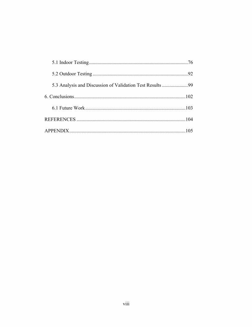
viii
5.1 Indoor Testing ................................................................................76
5.2 Outdoor Testing .............................................................................92
5.3 Analysis and Discussion of Validation Test Results .....................99
6. Conclusions ..........................................................................................102
6.1 Future Work .................................................................................103
REFERENCES ........................................................................................104
APPENDIX ..............................................................................................105

ix
LIST OF TABLES
2.1 Input and output signals of the Drivven ECU ........................................8
3.1 NIST scenarios used for initial oxygen estimation algorithm [7] ........24
3.2 NIST test scenarios used for final oxygen estimation algorithm .........26
3.3 New O2 estimation best fit cut times and estimation parameters .........46
3.4 Estimation parameters and sum of squared error (all algorithms) .......53
5.1 Load points used for validation testing at UA .....................................73
5.2 Operating conditions used for validation testing at UA .......................76
5.3 Summary of validation testing results at UA .....................................101

x
LIST OF FIGURES
2.1 Crank Position Sensor and 24 Tooth Crank Wheel ...............................9
2.2 Diagram of Drivven EMS ....................................................................10
2.3 EMS equipped Coleman Powermate 7000 Watt generator .................13
2.4 Delphi MT05 ECU mounted inside the generator frame [6] ...............18
2.5 NI cRIO-9022 Drivven based ECU mounted in protective box ..........20
3.1(a) Measured and calculated O2 percentages for Test N .......................30
3.1(b) New estimation parameters and sum of squared errors (Test N) ....30
3.2(a) Measured and calculated O2 percentages for Test T .......................31
3.2(b) New estimation parameters and sum of squared errors (Test T) .....31
3.3(a) Measured and calculated O2 percentages for Test Z .......................32
3.3(b) New estimation parameters and sum of squared errors (Test Z) .....32
3.4(a) Measured and calculated O2 percentages for Test W ......................33
3.4(b) New estimation parameters and sum of squared errors (Test W) ...33
3.5(a) Measured and calculated O2 percentages for Test AH ....................34
3.5(b) New estimation parameters and sum of squared errors (Test AH) .34
3.6(a) Measured and calculated O2 percentages for Test U .......................35
3.6(b) New estimation parameters and sum of squared errors (Test U) ....35
3.7(a) Measured and calculated O2 percentages for Test V .......................36
3.7(b) New estimation parameters and sum of squared errors (Test V) ....36

xi
3.8(a) Measured and calculated O2 percentages for Test AK ....................37
3.8(b) New estimation parameters and sum of squared errors (Test AK) .37
3.9(a) Measured and calculated O2 percentages for Test AS .....................38
3.9(b) New estimation parameters and sum of squared errors (Test AS) ..38
3.10(a) Measured and calculated O2 percentages for Test AV ..................39
3.10(b) New estimation parameters and sum of squared errors (Test AV)39
3.11(a) Measured and calculated O2 percentages for Test CA ..................40
3.11(b) New estimation parameters and sum of squared errors (Test CA)40
3.12(a) Measured and calculated O2 percentages for Test CB ..................41
3.12(b) New estimation parameters and sum of squared errors (Test CB) 41
3.13(a) Measured and calculated O2 percentages for Test CC ..................42
3.13(b) New estimation parameters and sum of squared errors (Test CC) 42
3.14(a) Measured and calculated O2 percentages for Test CD ..................43
3.14(b) New estimation parameters and sum of squared errors (Test CD)43
3.15(a) Measured and calculated O2 percentages for Test CE ...................44
3.15(b) New estimation parameters and sum of squared errors (Test CE) 44
3.16 Measured and calculated O2 percentages for concatenated tests .......49
3.17 Measured and calculated O2 percentages (different CAT estimates) 50
3.18(a) Measured and calculated O2 percentages (original and final) .......51
3.18(b) Final estimation parameters and sum of squared error (all tests) ..52
3.19 Calculated and estimated COHb levels for all tests ...........................56

xii
3.20 Oxygen depletion algorithm shutdown vs. ideal shutdown times .....58
3.21 COHb percetnages and measured CO at simulated shutdown ...........59
3.22 Measured CO emissions at actual and ideal shutdown times ............59
3.23 Oxygen estimations at actual and ideal shutdown times ...................60
3.24 Measured CO at actual and ideal shutdown times / maxiumum CO .60
3.25 Maximum CO for all indoor test cases ..............................................61
3.26 Estimated and actual COHb at shutdown / maximum COHb ............61
3.27 Maximum COHb (CPSC calculation) for all indoor test cases .........62
4.1 Individual area calculations (piecewise linear function) .....................66
4.2 Individual difference measurements (piecewise constant function) ....67
4.3 LabVIEW implementation of oxygen estimation algorithm in ECU ..71
4.4 LabVIEW implementation of shutdown algorithm in ECU ................71
5.1 Trailer used for indoor operation test scenarios ...................................73
5.2 Nova analyzer used to measure emissions in enclosed environment ..74
5.3(a) Oxygen estimation and oxygen measured for Test UA1 .................78
5.3(b) COHb estimation and CPSC COHb calculation for Test UA1 .......78
5.3(c) Measured CO emissions for Test UA1 ............................................79
5.3(d) Algorithm shutdown signal for Test UA1 .......................................79
5.4(a) Oxygen estimation and oxygen measured for Test UA2 .................80
5.4(b) COHb estimation and CPSC COHb calculation for Test UA2 .......80
5.4(c) Measured CO emissions for Test UA2 ............................................81

xiii
5.4(d) Algorithm shutdown signal for Test UA2 .......................................81
5.5(a) Oxygen estimation and oxygen measured for Test UA3 .................82
5.5(b) COHb estimation and CPSC COHb calculation for Test UA3 .......82
5.5(c) Measured CO emissions for Test UA3 ............................................83
5.5(d) Algorithm shutdown signal for Test UA3 .......................................83
5.6(a) Oxygen estimation and oxygen measured for Test UA4 .................84
5.6(b) COHb estimation and CPSC COHb calculation for Test UA4 .......84
5.6(c) Measured CO emissions for Test UA4 ............................................85
5.6(d) Algorithm shutdown signal for Test UA4 .......................................85
5.7(a) Oxygen estimation and oxygen measured for Test UA5 .................86
5.7(b) COHb estimation and CPSC COHb calculation for Test UA5 .......86
5.7(c) Measured CO emissions for Test UA5 ............................................87
5.7(d) Algorithm shutdown signal for Test UA5 .......................................87
5.8(a) Oxygen estimation and oxygen measured for Test UA6 .................88
5.8(b) COHb estimation and CPSC COHb calculation for Test UA6 .......88
5.8(c) Measured CO emissions for Test UA6 ............................................89
5.8(d) Algorithm shutdown signal for Test UA6 .......................................89
5.9(a) Oxygen estimation and oxygen measured for Test UA7 .................90
5.9(b) COHb estimation and CPSC COHb calculation for Test UA7 .......90
5.9(c) Measured CO emissions for Test UA7 ............................................91
5.9(d) Algorithm shutdown signal for Test UA7 .......................................91

xiv
5.10(a) Oxygen estimation and oxygen measured for Test UA8 ...............94
5.10(b) COHb estimation and CPSC COHb calculation for Test UA8 .....94
5.11(a) Oxygen estimation and oxygen measured for Test UA9 ...............95
5.11(b) COHb estimation and CPSC COHb calculation for Test UA9 .....95
5.12(a) Oxygen estimation and oxygen measured for Test UA10 .............96
5.12(b) COHb estimation and CPSC COHb calculation for Test UA10 ...96
5.13(a) Oxygen estimation and oxygen measured for Test UA11 .............97
5.13(b) COHb estimation and CPSC COHb calculation for Test UA11 ...97
5.14(a) Oxygen estimation and oxygen measured for Test UA12 .............98
5.14(b) COHb estimation and CPSC COHb calculation for Test UA12 ...98

1
CHAPTER 1
Introduction
Portable gasoline generators are generally utilized when there is a need for power in rural
areas and during power outages caused by common weather phenomena such as thunderstorms,
hurricanes, tornadoes, snow storms, etc. One major advantage of portable gasoline generators is
the ability to provide power to any entity, such as household appliances, that would otherwise be
useless during periods of power loss. Alternatively, a major disadvantage of such generators is
the fact that many people do not use them properly, which can lead to health risks, due to their
hazardous emissions. The dangerous byproduct emitted by gasoline powered generators is that
of carbon monoxide (CO), a resultant gas in their exhaust from incomplete combustion [1]. CO
is a deadly, colorless, odorless, and poisonous gas that will cause headache, fatigue, shortness of
breath, nausea, and dizziness depending on concentration level, length of exposure, and an
individual’s health condition [1]. Extensive CO exposures can eventually lead to permanent
health conditions and even death.
From 1999 to 2012, 591 non-fire carbon monoxide poisoning deaths, caused by portable
gasoline generators alone, were reported to the Consumer Product Safety Commission (CPSC)
[2]. Eighty-one percent of these deaths occurred in homes, including houses, mobile homes,
apartments, townhouses, attached structures to homes, detached structures at home locations, and
non-fixed location residences [2]. As CO related deaths from gasoline powered generators

2
remain prevalent, the need for increased safety precautions will persist as well. The large
number of deaths, caused by CO poisoning from gasoline portable generators, previously led
CPSC to contract with The University of Alabama (UA) in efforts to reduce overall CO
emissions and implement a safety shutdown feature which would terminate engine operation
when indoor operation, and thus a hazardous environment, is detected. While overall CO
emissions reduction was achieved during the previous contract, the safety shutdown feature
possessed several shortcomings that needed to be addressed.
During the previous contract with CPSC, work done by UA was centered on the goal of
safer gasoline powered generator operation, and thus reducing the number of CO related deaths
from such tools, by way of two main tasks. The first main task of the previous contract involved
improving the overall CO emissions from gasoline powered generators, thus improving air
quality in areas immediately surrounding such generators and reducing the risk of associated CO
poisoning. This particular task was completed by converting a carbureted gasoline powered
generator engine to a fuel-injected engine through means of removing the carburetor and
replacing it with an Engine Management System (EMS) and three-way catalyst. The EMS
allowed for significant reduction in CO emissions by controlling the quantity of fuel delivered to
the engine (as well as spark timing) in order to maintain the fuel-air mixture charge around the
stoichiometric point. The fuel mixture is considered to be stoichiometric when the ratio of the
mass of air to the mass of fuel, or air-fuel ratio (AFR), is approximately 14.6 to 1 for typical
gasoline. When the fuel mixture is stoichiometric, this means that there is just enough air to
completely burn the available fuel and complete the combustion process. The fuel mixture is
said to be lean if the AFR is greater than stoichiometric, which implies more air is present than
required to completely oxidize the fuel. Alternatively, the fuel mixture is said to be rich if the

3
AFR is less than stoichiometric, implying that not enough air is present to fully oxidize the fuel.
A general description of the EMS setup will be discussed further in Chapter 2. The three-way
catalyst allowed for a reduction in all three major emissions, Hydrocarbons (HC), Nitrogen
Oxide (NOx), and CO, provided a stoichiometric fuel mixture was maintained. The net reduction
in CO using the EMS and catalyst was 97% [6]. The second main task of the previous contract
involved the development and implementation of a safety shutdown feature on-board a gasoline
powered generator in the event that indoor operation, and a potentially hazardous environment,
was detected. This initial shutdown algorithm was based on post-processing of emissions data,
gathered from oxygen depletion test scenarios, which indicated that the intake air temperature
(IAT), block learn memory (BLM) correction factor, and fuel pulse width (FPW) particularly
showed significant change in such an environment [6]. These three variables were used to
produce three identical moving averages, while a counter was used to count the number of
instances that each particular variable exceeded a specified threshold. The safety shutdown
feature was to take effect, terminating engine operation, if all three variables exceeded their
specified threshold value at the same time. This initial shutdown algorithm demonstrated a proof
of concept, but needed improvement in several areas.
While work on the previous contract with CPSC resulted in significant reductions in CO
emissions, the objective of designing and implementing a safety shutdown feature showed
several areas for improvement. First, the previous shutdown algorithm was only a heuristic
procedure that relied solely on specific variables crossing set thresholds. Second, the previous
algorithm sometimes produced false-positive shutdowns with sudden and significant load
changes. Third, the response time of the previous algorithm proved to be somewhat slow under
certain load conditions. Specifically, light load conditions resulted in a significant delay in

4
shutdown time, in an enclosed environment, allowing the generator to run well past the desired
termination point. Furthermore, the algorithm would sometimes not trigger a shutdown when
operating indoors, even under a high load. Finally, the implementation of the previous shutdown
algorithm could not be adjusted after appropriate testing due to the proprietary nature of the
Delphi MT05 engine control unit (ECU), which will be discussed further in Chapter 2. These
needs for enhancement led CPSC to contract again with UA for design, implementation, testing,
and validation of a new safety shutdown algorithm.
This thesis resulted from the new contract between CPSC and UA, which focused around
design and implementation improvement of the safety shutdown feature for the previously used
Coleman Powermate 7000 gasoline powered generator. A literature search was conducted in an
attempt to find any previous relevant work in the way of gasoline powered generator automatic
shutdown; however, nothing was discovered directly pertaining to the automatic shutoff of a
gasoline powered generator without the use of an external emission gas sensor. The previously
used shutdown algorithm, which was designed based on threshold crossings of three particular
variables, was replaced with a new algorithm that would be based on estimating the oxygen (O2)
content of the intake air. The initial development of the new algorithm was based on post-
processing of data from the National Institute of Standards and Technology (NIST), which was
obtained from validation tests during the previous contract. It was determined that oxygen could
be estimated in a real-time manner by using a combination of charge air temperature (CAT), base
fuel pulse width (FPW), and final FPW in a linear relationship. Because the task was to detect
an oxygen depletion environment without the use of external O2 or CO sensors, an oxygen
estimation based algorithm was the most plausible idea for improvement. Furthermore, oxygen
estimation was used to develop a trend-oriented estimate of carboxyhemoglobin (COHb). COHb
5
is a combination of CO and hemoglobin that effectively decreases the oxygen-carrying capacity
of blood, providing an indicator of potential health risk dependent on CO concentration and
length of exposure [3]. Therefore, the trend-oriented estimate COHb was ultimately used to shut
down the generator if a specified threshold was exceeded for a significant amount of time. Upon
physical testing, it was determined that the oxygen depletion algorithm would, rather quickly,
automatically shut down the generator when an oxygen depleted environment was detected.
Development of the new shutdown algorithm, based on post-processing of previous data, is
discussed in Chapter 3, while test results and algorithm validation are covered in Chapter 6.
The oxygen depletion shutdown algorithm implementation process was refined during
work on the new contract. As the previous Delphi MT05 ECU lacked the ability to be
reconfigured, it was subsequently replaced by the Drivven based ECU and National Instruments
(NI) cRIO-9022 controller which could be modified for appropriate algorithm implementation
and adjustment [4, 5]. As opposed to sending the shutdown algorithm to Delphi for
implementation, which was necessary for work done on the previous contract, the newly
acquired Drivven system eliminates project downtime and allows for ease of algorithm
development and necessary modifications. The Drivven ECU was configured to mimic that of
the Delphi MT05 in the way of engine operation, calibration, and closed-loop control method.
The generator’s engine was calibrated for closed-loop control operation at a stoichiometric fuel
mixture for specific test load points. The closed-loop control operation utilizes an oxygen
sensor’s voltage signal to determine if the AFR is lean or rich. Based on the state of the AFR,
closed-loop control can compensate and force the AFR back to stoichiometric. This Drivven
based ECU, which will be further discussed in Chapter 4, provides increased capability over the
previous controller primarily by allowing additions to the existing ECU software.

6
The ultimate goal of this thesis was achieved by implementing an automatic safety
shutdown feature on a 7000 Watt gasoline powered generator, previously adjusted for lower CO
emissions, by modifying existing ECU software. The oxygen estimation based shutdown
algorithm showed success by producing no outdoor false-positive engine shutoffs. Although the
newly revised shutdown algorithm proved successful in an enclosed oxygen depleted
environment, shutdown did occur earlier than expected in all indoor test cases.

7
CHAPTER 2
The Engine Management System (EMS)
The gasoline powered engine’s EMS is intended for management of multiple engine tasks
such as engine position tracking and synchronization of engine fuel and spark timing [4]. The
Drivven based EMS for this project was to utilize a setup parallel with the previous project, as
described in [6, 7], with the addition of an improved ECU. Because the new oxygen depletion
shutdown algorithm is initially based on post-processing of data from the previous project’s
EMS, the basic management criteria were to remain constant including the engine operation and
control principles. Specifically, the EMS setup is comprised of the host personal computer (PC),
an upgraded ECU, electronic fuel injector (EFI), a fuel pump and pressure regulator, and ignition
coil, along with multiple sensors for continuous engine operation monitoring. The host PC is
used for human interfacing with the ECU to monitor and adjust engine specific parameters. The
ECU is an electronic based system with multiple inputs and multiple outputs used to enhance
engine performance. Specifically, the ECU is used to execute pre-programed calculations based
on data provided from engine sensors and is responsible for controlling associated outputs to
achieve desired engine operation. The list, shown below in Table 2.1, details the multiple inputs
and outputs to the Drivven based ECU, similar to the Delphi system list in [6].

8
Table 2.1 Input and output signals of the Drivven ECU
Signal Input / Output Type
Oil Temperature Input Analog Intake Air Temperature Input Analog
Manifold Absolute Pressure Input Analog Heated Oxygen Sensor Input Analog
Battery Voltage Input Analog Crank Position Input Pulse Fuel Injector Output Digital
Spark Coil Output Digital
Each of the individual inputs and outputs to the ECU serve a specific role in the overall
engine control scheme. The two ECU outputs, for the fuel injector and spark coil, together serve
a common purpose of permitting fuel delivery and spark timing for fuel ignition through means
of the EFI, fuel pump, fuel pressure regulator, and ignition coil. The heated oxygen sensor is
used to detect oxygen content in the exhaust gas and determine whether the fuel mixture is rich
or lean through means of a corresponding voltage signal. The oil temperature sensor is
responsible for monitoring the temperature of the engine’s oil. The intake air temperature sensor
is responsible for monitoring the temperature of the air entering the engine. These two sensors,
oil temperature and intake air temperature, provide signals that contribute to various calculations
and look-up tables for parameters which effect engine operation. The crank position sensor is a
variable reluctance (VR) sensor, used in conjunction with a 24 tooth (minus 1) crank wheel,
responsible for defining engine speed (RPM) and a crank position reference point. By
establishing a crank position reference point, essential engine parameters such as manifold
absolute pressure (MAP), fuel delivery, and spark timing can be evaluated. The crank position
sensor and 24 tooth crank wheel are shown in Figure 2.1 [6, 7].

9
Figure 2.1: Crank Position Sensor and 24 Tooth Crank Wheel.
Through variable reluctance, a pulse train voltage signal is produced by the 24 tooth
crank wheel by exciting the crank position sensor that has magnitude proportional to engine
speed. A missing tooth, or gap, on the crank wheel is used as a reference point by the crank
position sensor for determining several useful parameters. First, the missing tooth is used to
establish a reference point for determining when the piston is at top dead center (TDC). In the
present strategy, the positioning of the piston at TDC is inferred by the falling edge of the 9th
tooth after the gap on the 24 tooth crank wheel, due to its specific alignment with respect to the
engine. In addition, the missing tooth and crankshaft synchronization system are used to ensure
that, at minimum pressure on the engine’s intake stroke, MAP read crank angle can be
determined. Due to MAP signal fluctuation, caused by the single-cylinder engine, a MAP read
crank angle algorithm is required for establishing a common MAP determination point. The
MAP read crank angle is a function of speed and load, which requires a calibration look-up table.
Since MAP is the primary variable used to indicate load, MAP read crank angle, sampled once
per two engine revolutions at minimum pressure, is based upon MAP itself [6, 7]. A block

10
diagram, shown in Figure 2.2, illustrates the complete layout and flow of all the Drivven-based
EMS components including the host PC, real-time ECU, a connected chassis with four engine
control modules, and multiple inputs / outputs to the generator. All bold lines indicate a voltage
signal and all dashed lines indicate signals to or from engine control modules harbored in the
ECU chassis. Additional signals are labeled accordingly.
Compact RIO / Drivven ECU
Host PersonalComputer
RJ45 EthernetPort Connection
ECU PowerSupply
A/D ComboModule
Oxygen SensorModule
CrankPositionSensor
24 ToothCrankWheel
OilTemperature
Sensor
Intake AirTemperature
Sensor
ManifoldAbsolutePressureSensor
HeatedOxygenSensor
Port Fuel Injector(PFI) Driver
Module
FuelInjector
PressureRegulator
FuelPump
SparkDriver
Module
SparkCoil
12 V PowerSupply
FuelFuel
VariableReluctance
Figure 2.2: Diagram of Drivven EMS.

11
The attached chassis currently contains four Drivven modules for engine control and one
National Instruments (NI) module, not included in the EMS diagram, for additional data
acquisition. The four modules harbored in the chassis include the following: A/D Combo
Module Kit, Port Fuel Injector (PFI) Driver Module Kit, Spark Driver Module Kit, Oxygen
Sensor Module Kit, and Bidirectional Digital I/O Module. The A/D Combo Module Kit is
responsible for interfacing between any analog or digital inputs on the generator, such as those
sensors which indicate operating conditions. Specifically, the A/D Combo Module Kit converts
the generator oil temperature, intake air temperature, crank position sensor, and MAP sensor
from analog to digital signals, which can be monitored and utilized in separate calculations. The
PFI Driver Module Kit is used for driving low-impedance and high-impedance PFIs as well as
generator solenoid valves. Specifically, the main task of the PFI Driver Module Kit is to control
the generator’s fuel pump and fuel injector. The Spark Driver Module Kit is responsible for
controlling the spark coil, ensuring precise timing for correct engine synchronization. The
Oxygen Sensor Module Kit is responsible for interfacing with wide-band and narrow-band
oxygen sensors. Specifically, the Oxygen Sensor Module Kit is used for engine tuning, closed-
loop engine control, and data acquisition. The Bidirectional Digital I/O Module was acquired, in
addition to the four previous modules needed for engine control, in order to output digital signals
to an analog oscilloscope. This module allowed for rapid controller and engine debugging,
without having to modify and recompile the associated source code [4].
Each of the previously described control modules are accompanied by LabVIEW based
virtual instruments (VIs) which are programs that contain the source code used to operate and
control the associated hardware [11]. In addition, the Drivven system must utilize CalVIEW
Calibration software, necessary for establishing communications between the real-time kernel

12
and the host VI by means of managing all necessary data points and lookup tables. The host VI
is used to monitor and control any desired system input or output in a real-time manner. Open-
loop and closed-loop engine tuning for stoichiometric engine operation are also performed in the
host VI, in real-time, which makes it vital to the new Drivven ECU.
During the course of the previous contract, which involved the development of a low CO
emissions prototype generator and safety shutdown feature, two separate engine controllers were
utilized. An obsolete Delphi controller, the IMEC-168 ECU, was used for initial calibration,
testing, and developing the low CO emissions prototype generator. This particular ECU, used
with a 3-way catalyst, aided in the reduction of CO emissions from a portable gasoline powered
generator by 97% [6]. The Delphi MT05 ECU was used specifically for work completed on the
previous oxygen depletion shutdown algorithm, with the same gasoline powered generator
already modified for low CO emissions.
In an effort to improve enclosed operation detection and shutoff of the existing setup, the
new Drivven ECU was introduced to the previously used Coleman Powermate 7000 generator
rated at a continuous output of 7 kW. A photograph depicts the portable gasoline powered
generator equipped with EMS in Figure 2.3. As a replacement to the existing Delphi ECU and
MT05 controller, the advantageous Drivven based ECU and NI cRIO-9022 controller allows for
more real-time engine adjustments, as well as modifications and additions to the ECU.
Replacing the ECU was necessary; however, the spark coil and all sensors, used with the
previous Delphi MT05 ECU, were able to be reused with the upgraded Drivven ECU.

13
Figure 2.3: EMS equipped Coleman Powermate 7000 Watt generator.
2.1 Complete ECU Description
Two different engine controllers have been used throughout the course of the two
contracts with CPSC for the purpose of developing an oxygen depletion safety shutdown feature;
however, the fundamental bases upon which they operate are the same, as the Drivven ECU
utilizes a similar speed-density method as the previous Delphi MT05. A parallel deterministic
approach and set of principle equations are used, as described in [6, 7, 8], which utilize the
primary inputs of engine speed and a load variable, based on MAP, for ultimately controlling the
mass of fuel delivered. The speed-density method, based on the ideal gas law, is used to
calculate the quantity of air entering the engine, thus delivering a stoichiometric fuel mixture to
the engine. The ideal gas law is shown in Equation 2.1 where (P) is pressure, (V) is volume, (m)
is mass, (R) is the air gas constant, and (T) is temperature. The actual mass of air entering the
cylinder divided by the theoretical mass of air entering the cylinder is defined as the volumetric
efficiency, shown in Equation 2.2. As seen in Equation 2.2, the theoretical mass of air entering
the cylinder is equal to the product of the air density entering the cylinder (ρair) and the engine

14
displacement volume (VD). As part of the calibration procedure, the volumetric efficiency is
determined as a function of engine speed and load and entered into a lookup table for use by the
algorithm as part of the air flow calculation [6, 7].
TRmVP *** (2.1)
Dair
air
air
air
V
m
ltheoreticam
actualmVE
* (2.2)
Because the air is an ideal gas, a relationship with the ideal gas law can be developed.
Specifically, by combining Equation 2.1 with the fact that air density is defined by air mass
divided by air volume, the manifold air density can be calculated in terms of the specific
pressure, temperature, and air gas constant. The manifold density is directly proportional to the
manifold pressure (Pman) and inversely proportional to the manifold temperature (Tman), as shown
in Equation 2.3 [6, 7, 8].
man
manman TR
P
* (2.3)
Using the combination of Equations 2.2 and 2.3, equating air density entering the cylinder to
manifold air density, the actual mass of air entering the cylinder is calculated, as shown in
Equation 2.4, with respect to the specific manifold conditions. As described in [6], a unique
relationship between Equation 2.3 and the current EMS can be drawn by the following
parameters: Pman = MAP (kPa), VD = volume of the cylinder, 389 (cm3), R = air gas constant,
0.286 (kJ/[kg*K]), and Tman = charge air temperature (CAT) (°C). The CAT is a useful
calculation that estimates the air temperature entering the cylinder, based on experimental
correlation, which is dependent upon an RPM and MAP based coefficient lookup table, IAT, and
oil temperature (CLTS).
15
man
Dmanair TR
VEVPm
*
** (2.4)
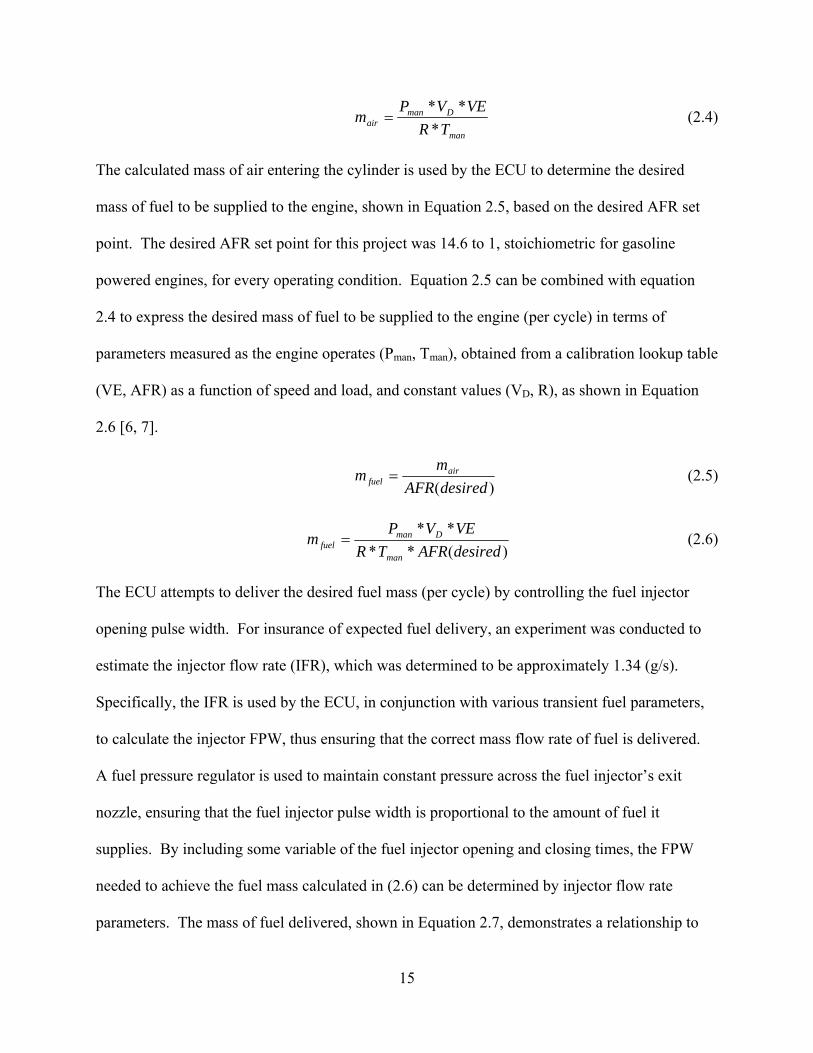
The calculated mass of air entering the cylinder is used by the ECU to determine the desired
mass of fuel to be supplied to the engine, shown in Equation 2.5, based on the desired AFR set
point. The desired AFR set point for this project was 14.6 to 1, stoichiometric for gasoline
powered engines, for every operating condition. Equation 2.5 can be combined with equation
2.4 to express the desired mass of fuel to be supplied to the engine (per cycle) in terms of
parameters measured as the engine operates (Pman, Tman), obtained from a calibration lookup table
(VE, AFR) as a function of speed and load, and constant values (VD, R), as shown in Equation
2.6 [6, 7].
)(desiredAFR
mm air
fuel (2.5)
)(**
**
desiredAFRTR
VEVPm
man
Dmanfuel (2.6)
The ECU attempts to deliver the desired fuel mass (per cycle) by controlling the fuel injector
opening pulse width. For insurance of expected fuel delivery, an experiment was conducted to
estimate the injector flow rate (IFR), which was determined to be approximately 1.34 (g/s).
Specifically, the IFR is used by the ECU, in conjunction with various transient fuel parameters,
to calculate the injector FPW, thus ensuring that the correct mass flow rate of fuel is delivered.
A fuel pressure regulator is used to maintain constant pressure across the fuel injector’s exit
nozzle, ensuring that the fuel injector pulse width is proportional to the amount of fuel it
supplies. By including some variable of the fuel injector opening and closing times, the FPW
needed to achieve the fuel mass calculated in (2.6) can be determined by injector flow rate
parameters. The mass of fuel delivered, shown in Equation 2.7, demonstrates a relationship to

16
the IFR, the FPW time (tFPW), and the FPW time correction (tC), used to account for time needed
to fully open the injector and close the injector. Furthermore, by equating the mass of fuel
delivered in (2.7) to the desired mass of fuel in (2.6), the FPW time needed to supply the desired
mass of fuel can be calculated, as shown in Equation 2.8 [6,7].
CFPWdelfuel ttIFRm *, (2.7)
Cman
DmanFPW t
IFRdesiredAFRTR
VEVPt
*)(**
** (2.8)
In order to control the engine around a stoichiometric fuel mixture, the same closed-loop
control (CLC) algorithm from the Delphi MT05 controller was used in the newly acquired
Drivven ECU. Initially, the system will run in open-loop mode until temperature and run time
thresholds have been achieved which activates CLC. These particular thresholds were extracted
from the Delphi system; however, the Drivven system allows for CLC to be initiated at the user’s
discretion if a scenario arises which calls for CLC to be activated sooner or later than normal.
An oxygen sensor, placed in the exhaust stream, acts as a feedback signal for the closed-loop
control algorithm, sensing either a fuel rich or fuel lean mixture. Accordingly, the calculated
fuel pulse width time is adjusted so the oxygen signal constantly switches between rich and lean,
ensuring the fuel mixture is always near stoichiometric. A proportional-integral (PI) control
method was used to ensure that the AFR constantly oscillated around stoichiometric. The
proportional component of the controller is responsible for the size of the FPW adjustment,
which is determined by the magnitude of the difference between the actual and desired
conditions. Essentially, the proportional factor uses the oxygen sensor feedback to constantly
vary the fuel mixture between rich and lean. The integral component is responsible for ensuring
that an event, or particular value, will eventually occur by constantly adjusting until the feedback
signal surpasses a set value. Therefore, the integral factor increases for a lean fuel mixture and

17
decreases for a rich fuel mixture, ensuring that the controller maintains an AFR near 14.6 to 1.
Finally, the proportional and integral corrections are applied to the FPW after each calculation
and the control process is subsequently repeated. Gain coefficients must be adjusted for both the
proportional and integral components, located in a lookup table based on engine speed and load,
in order to ensure quick and accurate corrections are made by the controller adjustments [6, 7].
The new Drivven ECU is modified to emulate engine operation and control of the previous
Delphi ECU; however, the subsequent subsections discuss how each controller remains unique.
2.1.1 Delphi MT05 ECU Description
As described in [6], the previously used Delphi MT05 ECU, shown in Figure 2.4, was a
replacement, and upgrade, for the obsolete Delphi IMEC-168 ECU. The MT05 ECU provided a
slimmer design, which allowed for the controller to be mounted inside of the generator frame,
helping to eliminate unintended damage. Also, the MT05 ECU utilized an external MAP sensor,
unlike its predecessor, in order to increase the MAP signal consistency from the previous system.
By using a MAP tube, the external MAP sensor was placed above the engine’s existing MAP
port. Allowing for a more reliable MAP signal was vital, as it is used for calculating many
engine control parameters.

18
Figure 2.4: Delphi MT05 ECU mounted inside the generator frame [6].
The Delphi MT05 ECU possessed a 20 MHz microprocessor with 512 bytes of EEPROM
memory space and 256 Kbytes of flash EEPROM memory space. A controller area network
(CAN) was used as communication link between the ECU and laptop computer. The Delphi
software contained a calibration toolbox which was used for real-time data logging, data
playback, and exporting data. As previously mentioned, the Delphi system utilized an external
MAP sensor, as well as a heated oxygen sensor. Also, an upgrade on the MT05 ECU was the
ability to modify the look-up table axes for improved engine performance [6, 9]. As the MT05
ECU served as a substantial upgrade from the Delphi IMEC-168 ECU, it still lacked the ability
to be modified as an open-source controller. Upon completion of the previous oxygen depletion
shutdown algorithm, based on post-processing of data, a submission to Delphi was required for
implementation. This eliminated the possibility of shutdown algorithm modification based on
current test data.

19
2.1.2 NI cRIO-9022 Drivven based ECU Description
The newly acquired Drivven EMS controller, shown in Figure 2.5, is based on a National
Instruments Compact RIO (reconfigurable input / output) NI cRIO-9022 which allows for real-
time deterministic control, data logging, and a wide variety of engine management tasks such as
tracking engine position and engine synchronization of fuel delivery and spark control. These
ECU operations are based on field programmable gate arrays (FPGA) [4, 5]. Figure 2.5 also
depicts the attached chassis with four Drivven engine control modules and one NI module for
additional data acquisition. The primary advantage of the Drivven ECU is that it is a mostly
open-source controller that provides the ability for modifications and additions to the existing
ECU source code through the LabVIEW-based software which accompanies each individual
control module present in the chassis. In addition, the Drivven ECU still possessed the main
upgrade features to the previous MT05 ECU such as an external MAP sensor and the ability to
modify the look-up table axes for increased resolution and engine performance. One notable
difference from the previous Delphi MT05 ECU is the Drivven system’s location with respect to
the generator itself. Due to the Drivven system’s larger size, it cannot be mounted directly on
the generator and must be placed inside of a protective box, as shown in Figure 2.5, to limit
exposure to potentially harmful elements and prevent any accidental damage. Although not a
subject of this thesis, it is worth noting that the finished product for engine operation, control,
and new safety shutdown algorithm were implemented on a smaller, less complex, and less
expensive controller, intended only for use after all desired modifications had been finalized.
This allowed for ease of ECU modifications with the Drivven system, while final implantation
on a smaller controller allowed for the final product to be mounted on the generator.

20
Figure 2.5: NI cRIO-9022 Drivven based ECU mounted in protective box.
The NI cRIO-9022 and Drivven based ECU possesses a 533 MHz processor with 2
Gbytes of nonvolatile storage and 256 Mbytes of dynamic random-access memory (DRAM).
The real-time kernel operates at 1 kHz, while the FPGA kernel operates at 40 MHz for more
time-critical engine operations. The controller itself has several different external connection
capabilities such as multiple Ethernet ports for remote interfacing with the host PC and file
servers, a USB port for hosting external memory devices, and RS232 serial port connection
which could be used as to communicate between the ECU and peripherals. The controller is
designed to function for long periods of time, at low power consumption, and a wide operating
temperature range [5].
The Drivven EMS and ECU was modified in hardware and software to emulate that of
the previous MT05 controller as closely as practically possible. The Drivven ECU was
originally designed for a multi-cylinder engine, while the generator used for this project utilized
a single-cylinder engine. Therefore, due to the Drivven ECU’s ability to be reconfigured, the
ECU was modified in order to accommodate a single-cylinder engine. In order to begin this

21
modification, the associated LabVIEW code in the Drivven ECU was altered in the way of
disabling the three additional cylinders needed for four-cylinder operation. In addition, the
engine design warranted the previously discussed MAP read crank angle algorithm to be
implemented for determining MAP at a common point, the minimum pressure read once every
two engine revolutions. Due to the generator’s absence of a cam sensor, a pseudo cam signal
algorithm was implemented in the ECU, using LabVIEW code, which would emulate that of a
physical cam signal. A physical cam sensor produces a true signal synchronized with the
camshaft which can be combined with the crank position sensor to establish crank position
relative to the complete four-stroke engine cycle. One important calculation that was performed
by the previous MT05 controller, missing in the Drivven ECU, was the CAT calculation.
Therefore, necessary additions were made to the Drivven ECU software to perform the CAT
calculation. CAT is absolutely vital because of the fact that oxygen estimation and the
emergency engine shutdown algorithm, discussed in the following chapter, are dependent upon
the temperature estimation. The final modification to the Drivven ECU was the implementation
of the previously discussed CLC algorithm used in the previous MT05 controller to control the
AFR to stoichiometric.

22
CHAPTER 3
Oxygen Depletion Shutdown Algorithm
During work done in this project’s previous phase, an oxygen depletion shutdown
algorithm was developed that, although demonstrated a proof of concept, possessed
shortcomings which needed to be addressed. Specifically, the previous shutdown algorithm was
only a heuristically based model which did not address the air chemistry directly related to an
oxygen depleted environment. Also, the previous algorithm sometimes produced false-positive
shutdowns with sudden and significant load changes. Finally, the previous algorithm possessed
issues concerning the shutdown feature’s response time. Under light load conditions, in an
enclosed environment, a significant delay in shutdown time allowed the generator to continue
running past the desired termination point.
In an effort to improve the oxygen depletion safety shutdown feature, an advanced
algorithm was devised by attempting to approximately estimate the oxygen percentage in a
gasoline portable generator’s intake air without the use of any external emission sensors. While
several numerical estimation methods proved unsuccessful, a hybrid analytical and heuristic
strategy demonstrated some promising results. The general purpose of this strategy was to be
able to generate a curve that matched the oxygen data measured throughout testing at the NIST
test facility. It was determined that by utilizing the gas constant for air, the actual gas constant at
the generator’s air intake, expected fuel-air ratio, and actual fuel-air ratio, a useful relationship

23
could be derived to estimate the amount of oxygen in the air intake stream if the small injector
opening or closing times were neglected. In the ECU, the base FPW is calculated by using the
gas constant for air and a desired air-fuel mixture ratio. Then, through control system feedback,
the actual gas constant at the generator’s air intake could be calculated based on the actual FPW
corrected by the controller, also known as the final FPW. Also, the actual fuel-air ratio could be
determined once the control system corrections are made. Through some mathematical
simplification, the ratios of the actual intake air gas constant to the gas constant for air and
expected fuel-air ratio to actual fuel-air ratio are used to provide a useful FPW ratio for oxygen
estimation, as shown in Equation 3.1 [7].
finalFPW
baseFPW
air
actual
actual t
t
R
R
AF
AF
,
,exp
(3.1)
This ratio proved useful for developing a strategy to estimate the oxygen percentage in the
generator’s air intake stream. In fact, a measure of control system correction, for oxygen
deficiency in the intake gas stream, is described by this ratio of base FPW to final FPW. Over
the course of several NIST testing procedures, it was observed that the ratio described in
Equation 3.1, in conjunction with the generator’s calculated CAT, could be used as a constant
parameter in a linear oxygen estimation equation. In particular, this constant value (C) used for
linear estimation is described by the ratio shown in Equation 3.2. In addition, it was determined
that a basis of this constant value was able to more accurately estimate oxygen once the CAT
stabilized [7].
CATt
tC
finalFPW
baseFPW
*,
, (3.2)
24
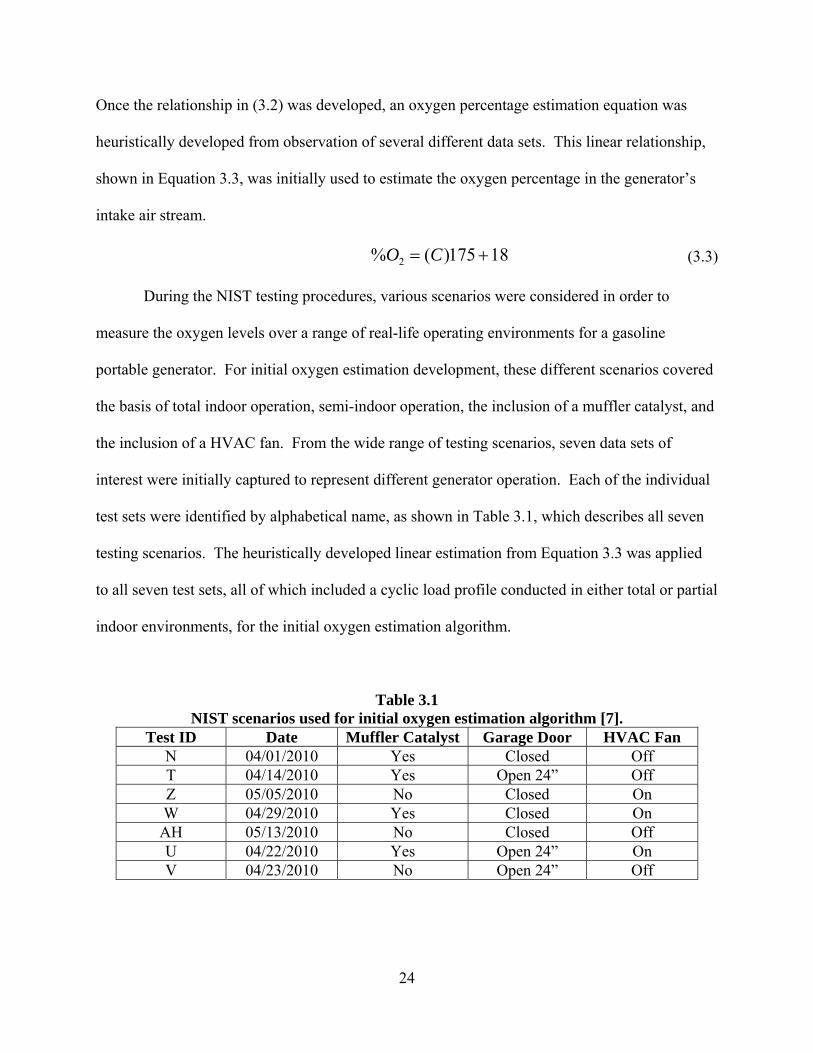
Once the relationship in (3.2) was developed, an oxygen percentage estimation equation was
heuristically developed from observation of several different data sets. This linear relationship,
shown in Equation 3.3, was initially used to estimate the oxygen percentage in the generator’s
intake air stream.
18175)(% 2 CO (3.3)
During the NIST testing procedures, various scenarios were considered in order to
measure the oxygen levels over a range of real-life operating environments for a gasoline
portable generator. For initial oxygen estimation development, these different scenarios covered
the basis of total indoor operation, semi-indoor operation, the inclusion of a muffler catalyst, and
the inclusion of a HVAC fan. From the wide range of testing scenarios, seven data sets of
interest were initially captured to represent different generator operation. Each of the individual
test sets were identified by alphabetical name, as shown in Table 3.1, which describes all seven
testing scenarios. The heuristically developed linear estimation from Equation 3.3 was applied
to all seven test sets, all of which included a cyclic load profile conducted in either total or partial
indoor environments, for the initial oxygen estimation algorithm.
Table 3.1 NIST scenarios used for initial oxygen estimation algorithm [7].
Test ID Date Muffler Catalyst Garage Door HVAC Fan N 04/01/2010 Yes Closed Off T 04/14/2010 Yes Open 24” Off Z 05/05/2010 No Closed On W 04/29/2010 Yes Closed On AH 05/13/2010 No Closed Off U 04/22/2010 Yes Open 24” On V 04/23/2010 No Open 24” Off
25
The initial oxygen estimation algorithm, developed for purposes of an advanced
shutdown algorithm, showed some promising results in generating a curve to estimate the
oxygen content measured during NIST testing. However, due to the fact that the linear
estimation in Equation 3.3 was heuristically developed, it was decided that the oxygen
percentage levels could be calculated more accurately if new linear coefficients, other than 175
and 18, were mathematically derived. Also, because of the fact that all seven test sets, used to
initially develop the new algorithm, were conducted indoors under a cyclic load profile, it was of
particular interest to broaden the real-life operation spectrum by including indoor constant load
tests and outdoor tests. The processes of developing the new optimum linear estimation
coefficients, criteria for generator shutdown decision, and off-line validation are described in the
subsequent sections.
3.1 Method of Least Squares for Linear Curve Fitting
Due to the fact that the two coefficients, 175 and 18, in the initial linear oxygen
estimation equation (3.3) were heuristically developed in previous work, it was of particular
interest in the project’s current phase to mathematically derive new coefficients that would
represent a more accurate linear estimation. In addition, the test sets used in the initial oxygen
estimation algorithm were performed with several variables, such as a muffler catalyst, HVAC
fan, and total / partial indoor operation. However, it became of particular interest to ensure that
all operating conditions were accounted for in the way of indoor / outdoor test environment and
constant / cyclic load profile to ensure that oxygen estimation was as accurate as possible for any
real-life operating scenario. Therefore, eight additional cases from NIST testing were included,
with the seven existing cases, to result in fifteen total test sets which would represent a

26
broadened range of real-life operating conditions. These fifteen test cases, used in determining
the new optimal oxygen estimation coefficients, are listed in Table 3.2.
Table 3.2 NIST test scenarios used for final oxygen estimation algorithm.
Test ID Date Load Profile Environment Garage Door N 04/01/2010 Cyclic Indoors Closed T 04/14/2010 Cyclic Indoors Open 24” Z 05/05/2010 Cyclic Indoors Closed W 04/29/2010 Cyclic Indoors Closed AH 05/13/2010 Cyclic Indoors Closed U 04/22/2010 Cyclic Indoors Open 24” V 04/23/2010 Cyclic Indoors Open 24”
AK 05/19/2010 5500 W Indoors Fully Open AS 06/10/2010 5500 W Indoors Closed AV 07/09/2010 500 W Indoors Closed CA 09/10/2010 2500 W Outdoors CB 09/10/2010 1500 W Outdoors CC 09/10/2010 3000 W Outdoors CD 09/10/2010 4500 W Outdoors CE 09/10/2010 5500 W Outdoors
In order to achieve the two new coefficients that would most accurately estimate the
oxygen percentage in the generator’s intake air, for a broad spectrum of operating conditions, a
linear best fit algorithm was employed. To begin, the linear mathematical relationship shown in
Equation 3.4 was used to generally describe the estimated oxygen percentage, where k1 and k2
would represent the new coefficients, or estimation parameters.
212 )(% kkCO (3.4)
Using this generalized linear equation, an algorithm was implemented using the
MATLAB software environment to determine new estimation parameters that would produce the
most accurate oxygen calculation [10]. For the purpose of implementing the generalized oxygen

27
equation (3.4) into MATLAB software, the resulting matrix form of the linear estimation
equation, shown in Equation 3.5, was developed.
kCO
*][ (3.5)
In order to obtain a best fit calculation, the method of least squares was performed in MATLAB
by manipulating the generalized equation in (3.5) to solve for the estimation parameters. The (C)
matrix represented the generator data as described in equation 3.2 and would possess dimensions
of (n x 2), where n represents the number of samples. Specifically, one column would contain
the generator data from equation 3.2 while the other column would act as a place-holder filled
with ones. The oxygen percentage variable (the O vector), would represent the measured oxygen
data, in order to obtain the least squared error between the oxygen estimation and the actual
oxygen content, and would possess dimensions of (n x 1). Due to the fact that the measured
oxygen data only possessed a rate of 1 sample per 360 seconds (s), there were a limited number
of data points that could be utilized in the least squares curve fitting algorithm. Solving for the
new estimation parameters (the k vector), with dimensions of (2 x 1), and accounting for matrix
multiplication dimension requirements yielded the matrix form equation shown in Equation 3.6.
OCCCk TT
][][][1
(3.6)
Each of the fifteen previously mentioned test sets was individually analyzed using the
new parameter estimation algorithm (least squares method) to calculate more accurate linear
estimation coefficients. To determine the most accurate estimation parameters, several statistical
factors were considered. In particular, two significant factors arose while observing the
calculated data curves and attempting to derive more accurate estimation parameters: 1) the
transient period of the calculated data, and 2) the amount of error that exists, between the
measured and calculated data, once the transient phase was over. In order to derive estimation

28
parameters which most accurately calculated the oxygen percentage in the intake air, for the
large majority of time, data cut times were employed in increments of 360 s to clip the data
previous to the prescribed cut time. Once the transient period of the calculated data was
eliminated, a better linear curve fit was achieved by deriving new estimation parameters for
every possible remaining cut time. In order to statistically verify which cut time and new
estimation parameters provided an optimum linear curve fit to the measured oxygen data, a sum
of squared error measure was employed. The squared error was calculated at every sample
point, from the current cut time to the end of the test, by squaring the difference, or error,
between estimated oxygen and measured oxygen. Once all sample points had been considered,
the squared errors were added together to produce a sum of squared error for each cut time.
Using each possible individual cut time, and each individual new set of estimation parameters, a
new individual oxygen percentage calculation was created which spanned the test’s entire time
scale. From each new calculation, the sum of squared error was measured, once the transient
period was over, between the following data sets: 1) the raw oxygen calculation and measured
oxygen data, and 2) the filtered oxygen calculation and the measured oxygen data. Filtered
oxygen calculation curves were generated using a first-order lag filter to reduce the large
variations that existed in raw oxygen calculation curves.
The following plots, Figures 3.1 through 3.15, graphically illustrate several important
factors, relevant to determining the optimum linear estimation parameters for each individual test
set. For each data set, part (a) of the figure illustrates the measured oxygen data (in blue), plotted
along with the original filtered oxygen linear estimation (in green), from Equation 3.3, and the
new best fit filtered oxygen linear estimation (in red), generated by the least squares algorithm.
Measured oxygen for outdoor tests, CA through CE, was assumed to be 21% oxygen,

29
approximately ambient air. The new estimation parameters would differ significantly between
test sets, due to various generator operating environments; however, the long-term goal was to
achieve the most accurate pair of estimation parameters to fit the full scale of all fifteen
combined test sets. In addition, the newly derived estimation parameters, k1 and k2 (in blue and
green, respectively), and sum of squared errors, for the filtered curve fit and raw curve fit (in
blue and green, respectively), are plotted against all possible cut times in part (b) of each figure.

30
0 1000 2000 3000 4000 5000 6000 700018
19
20
21
22
23
24
Time (s)
%O
2
Oxygen Percentages
meas
orig calc filtfilterd curve fit
Figure 3.1(a): Measured and calculated O2 percentages for Test N.
0 1000 2000 3000 4000 5000 6000 7000 80000
50
100
150
Cut Time (s)
k1
k1
k2
0 1000 2000 3000 4000 5000 6000 7000 800017
18
19
20
k2
New O2 Estimation Parameters
0 1000 2000 3000 4000 5000 6000 7000 80000
0.5
1
1.5
Cut Time (s)
Err
or
Sum of Squared Errors
sum of sq error vs. filt line
sum of sq error vs. raw line
Figure 3.1(b): New estimation parameters and sum of squared errors (Test N).

31
0 2000 4000 6000 8000 1000018
19
20
21
22
23
24
Time (s)
%O
2
Oxygen Percentages
meas
orig calc filtfilterd curve fit
Figure 3.2(a): Measured and calculated O2 percentages for Test T.
0 2000 4000 6000 8000 10000 12000-5
0
5
10
Cut Time (s)
k1
k1
k2
0 2000 4000 6000 8000 10000 1200020.85
20.9
20.95
21
k2
New O2 Estimation Parameters
0 2000 4000 6000 8000 10000 120000.015
0.02
0.025
0.03
0.035
0.04
Cut Time (s)
Err
or
Sum of Squared Errors
sum of sq error vs. filt line
sum of sq error vs. raw line
Figure 3.2(b): New estimation parameters and sum of squared errors (Test T).

32
0 500 1000 1500 2000 2500 3000 3500 400018
19
20
21
22
23
24
Time (s)
%O
2
Oxygen Percentages
meas
orig calc filtfilterd curve fit
Figure 3.3(a): Measured and calculated O2 percentages for Test Z.
0 500 1000 1500 2000 2500 3000 3500 40000
100
200
Cut Time (s)
k1
k1
k2
0 500 1000 1500 2000 2500 3000 3500 400018
19
20
k2
New O2 Estimation Parameters
0 500 1000 1500 2000 2500 3000 3500 40000
0.2
0.4
0.6
0.8
Cut Time (s)
Err
or
Sum of Squared Errors
sum of sq error vs. filt line
sum of sq error vs. raw line
Figure 3.3(b): New estimation parameters and sum of squared errors (Test Z).

33
0 0.2 0.4 0.6 0.8 1 1.2 1.4 1.6 1.8 2
x 104
15
16
17
18
19
20
21
22
23
24
25
Time (s)
%O
2
Oxygen Percentages
meas
orig calc filtfilterd curve fit
Figure 3.4(a): Measured and calculated O2 percentages for Test W.
0 0.5 1 1.5 2 2.5
x 104
-500
0
500
Cut Time (s)
k1
k1
k2
0 0.5 1 1.5 2 2.5
x 104
16
18
20
k2
New O2 Estimation Parameters
0 0.5 1 1.5 2 2.5
x 104
0
10
20
30
40
Cut Time (s)
Err
or
Sum of Squared Errors
sum of sq error vs. filt line
sum of sq error vs. raw line
Figure 3.4(b): New estimation parameters and sum of squared errors (Test W).

34
0 2000 4000 6000 8000 10000 12000 14000 16000 1800015
16
17
18
19
20
21
22
23
24
25
Time (s)
%O
2
Oxygen Percentages
meas
orig calc filtfilterd curve fit
Figure 3.5(a): Measured and calculated O2 percentages for Test AH.
0 2000 4000 6000 8000 10000 12000 14000 16000 18000-100
0
100
200
300
Cut Time (s)
k1
k1
k2
0 2000 4000 6000 8000 10000 12000 14000 16000 1800016
16.5
17
17.5
18
k2
New O2 Estimation Parameters
0 2000 4000 6000 8000 10000 12000 14000 16000 180000
10
20
30
40
Cut Time (s)
Err
or
Sum of Squared Errors
sum of sq error vs. filt line
sum of sq error vs. raw line
Figure 3.5(b): New estimation parameters and sum of squared errors (Test AH).
35
0 500 1000 1500 2000 2500 3000 3500 4000 450018
19
20
21
22
23
24
Time (s)
%O
2
Oxygen Percentages
meas
orig calc filtfilterd curve fit
Figure 3.6(a): Measured and calculated O2 percentages for Test U.
0 500 1000 1500 2000 2500 3000 3500 4000 4500-10
0
10
20
30
40
Cut Time (s)
k1
k1
k2
0 500 1000 1500 2000 2500 3000 3500 4000 450020.4
20.6
20.8
21
21.2
21.4
k2
New O2 Estimation Parameters
0 500 1000 1500 2000 2500 3000 3500 4000 45000
0.05
0.1
0.15
0.2
Cut Time (s)
Err
or
Sum of Squared Errors
sum of sq error vs. filt line
sum of sq error vs. raw line
Figure 3.6(b): New estimation parameters and sum of squared errors (Test U).

36
0 1000 2000 3000 4000 5000 6000 7000 800018
19
20
21
22
23
24
Time (s)
%O
2
Oxygen Percentages
meas
orig calc filtfilterd curve fit
Figure 3.7(a): Measured and calculated O2 percentages for Test V.
0 1000 2000 3000 4000 5000 6000 7000 8000 9000-2
-1
0
1
2
3
Cut Time (s)
k1
k1
k2
0 1000 2000 3000 4000 5000 6000 7000 8000 900020.915
20.92
20.925
20.93
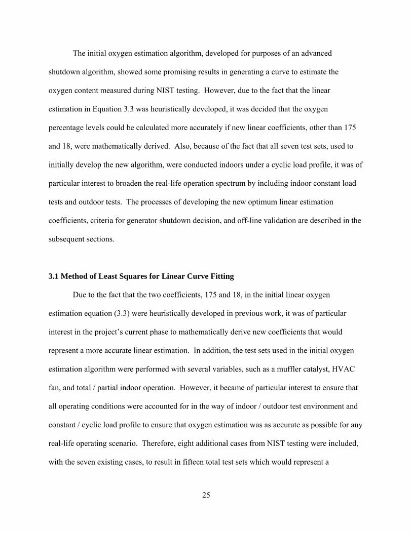
20.935
20.94
k2
New O2 Estimation Parameters
0 1000 2000 3000 4000 5000 6000 7000 8000 90000
0.01
0.02
0.03
0.04
0.05
0.06
Cut Time (s)
Err
or
Sum of Squared Errors
sum of sq error vs. filt line
sum of sq error vs. raw line
Figure 3.7(b): New estimation parameters and sum of squared errors (Test V).

37
0 500 1000 1500 2000 2500 3000 3500 4000 450018
19
20
21
22
23
24
Time (s)
%O
2
Oxygen Percentages
meas
orig calc filtfilterd curve fit
Figure 3.8(a): Measured and calculated O2 percentages for Test AK.
0 500 1000 1500 2000 2500 3000 3500 4000 4500 5000-15
-10
-5
0
5
Cut Time (s)
k1
0 500 1000 1500 2000 2500 3000 3500 4000 4500 500021.1
21.2
21.3
21.4
21.5
k2
New O2 Estimation Parameters
0 500 1000 1500 2000 2500 3000 3500 4000 4500 50002
2.5
3
3.5
4x 10
-3
Cut Time (s)
Err
or
Sum of Squared Errors
sum of sq error vs. filt line
sum of sq error vs. raw line
k1
k2
Figure 3.8(b): New estimation parameters and sum of squared errors (Test AK).

38
0 2000 4000 6000 8000 10000 1200018
19
20
21
22
23
24
Time (s)
%O
2
Oxygen Percentages
meas
orig calc filtfilterd curve fit
Figure 3.9(a): Measured and calculated O2 percentages for Test AS.
0 2000 4000 6000 8000 10000 12000 140000
200
400
Cut Time (s)
k1
0 2000 4000 6000 8000 10000 12000 1400016
18
20
k2
New O2 Estimation Parameters
0 2000 4000 6000 8000 10000 12000 140000
2
4
6
8
Cut Time (s)
Err
or
Sum of Squared Errors
sum of sq error vs. filt line
sum of sq error vs. raw line
k1
k2
Figure 3.9(b): New estimation parameters and sum of squared errors (Test AS).

39
0 1000 2000 3000 4000 5000 6000 700018
19
20
21
22
23
24
Time (s)
%O
2
Oxygen Percentages
meas
orig calc filtfilterd curve fit
Figure 3.10(a): Measured and calculated O2 percentages for Test AV.
0 1000 2000 3000 4000 5000 6000 7000-100
0
100
200
300
Cut Time (s)
k1
k1
k2
0 1000 2000 3000 4000 5000 6000 700017
18
19
20
21
k2
New O2 Estimation Parameters
0 1000 2000 3000 4000 5000 6000 70000
0.2
0.4
0.6
0.8
1
Cut Time (s)
Err
or
Sum of Squared Errors
sum of sq error vs. filt line
sum of sq error vs. raw line
Figure 3.10(b): New estimation parameters and sum of squared errors (Test AV).
40
0 500 1000 1500 2000 2500 300018
19
20
21
22
23
24
Time (s)
%O
2
Oxygen Percentages
meas
orig calc filtfilterd curve fit
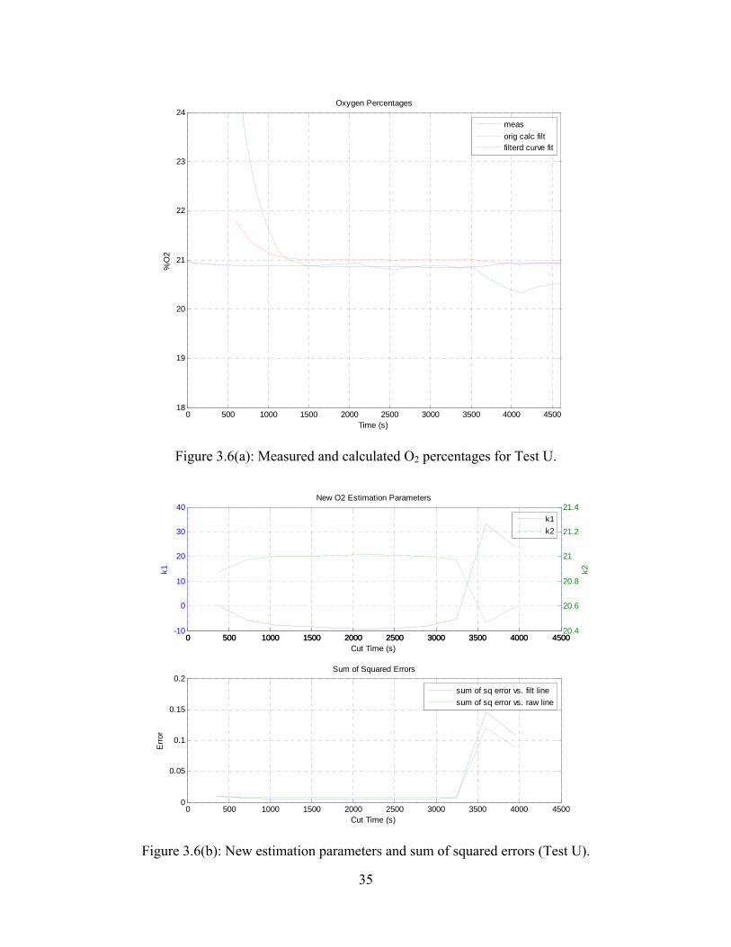
Figure 3.11(a): Measured and calculated O2 percentages for Test CA.
0 500 1000 1500 2000 2500 3000 3500-1
0
1
2
3
4x 10
-8
Cut Time (s)
k1
0 500 1000 1500 2000 2500 3000 350021
21
21
21
21
21
k2
New O2 Estimation Parameters
0 500 1000 1500 2000 2500 3000 35000
0.2
0.4
0.6
0.8
1
1.2x 10
-18
Cut Time (s)
Err
or
Sum of Squared Errors
sum of sq error vs. filt line
sum of sq error vs. raw line
k1
k2
Figure 3.11(b): New estimation parameters and sum of squared errors (Test CA).

41
0 200 400 600 800 1000 1200 1400 160018
19
20
21
22
23
24
Time (s)
%O
2
Oxygen Percentages
meas
orig calc filtfilterd curve fit
Figure 3.12(a): Measured and calculated O2 percentages for Test CB.
0 500 1000 1500-1
0
1
2
3
4x 10
-10
Cut Time (s)
k1
0 500 1000 150021
21
21
21
21
21
k2
New O2 Estimation Parameters
0 500 1000 15000
1
2
3
4x 10
-23
Cut Time (s)
Err
or
Sum of Squared Errors
sum of sq error vs. filt line
sum of sq error vs. raw line
k1
k2
Figure 3.12(b): New estimation parameters and sum of squared errors (Test CB).
42
0 200 400 600 800 1000 1200 1400 160018
19
20
21
22
23
24
Time (s)
%O
2
Oxygen Percentages
meas
orig calc filtfilterd curve fit
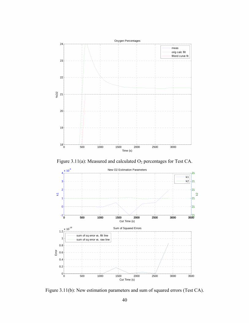
Figure 3.13(a): Measured and calculated O2 percentages for Test CC.
0 500 1000 15000
1
2
3
4
5x 10
-9
Cut Time (s)
k1
0 500 1000 150021
21
21
21
21
21
k2
New O2 Estimation Parameters
0 500 1000 15000
0.5
1
1.5
2
2.5x 10
-21
Cut Time (s)
Err
or
Sum of Squared Errors
sum of sq error vs. filt line
sum of sq error vs. raw line
k1
k2
Figure 3.13(b): New estimation parameters and sum of squared errors (Test CC).

43
0 100 200 300 400 500 600 700 800 90018
19
20
21
22
23
24
Time (s)
%O
2
Oxygen Percentages
meas
orig calc filtfilterd curve fit
Figure 3.14(a): Measured and calculated O2 percentages for Test CD.
0 100 200 300 400 500 600 700 800-3
-2
-1
0x 10
-11
Cut Time (s)
k1
0 100 200 300 400 500 600 700 80021
21
21
21
k2
New O2 Estimation Parameters
0 100 200 300 400 500 600 700 800-1
-0.5
0
0.5
1
Cut Time (s)
Err
or
Sum of Squared Errors
sum of sq error vs. filt line
sum of sq error vs. raw line
k1
k2
Figure 3.14(b): New estimation parameters and sum of squared errors (Test CD).

44
0 500 1000 1500 2000 2500 3000 3500 4000 4500 500018
19
20
21
22
23
24
Time (s)
%O
2
Oxygen Percentages
meas
orig calc filtfilterd curve fit
Figure 3.15(a): Measured and calculated O2 percentages for Test CE.
0 1000 2000 3000 4000 5000 6000-5
-4
-3
-2
-1
0
1
2
3
4
5x 10
-9
Cut Time (s)
k1
0 1000 2000 3000 4000 5000 600021
21
21
21
21
21
21
21
21
21
21
k2
New O2 Estimation Parameters
0 1000 2000 3000 4000 5000 60000
0.5
1
1.5
2
2.5x 10
-19
Cut Time (s)
Err
or
Sum of Squared Errors
sum of sq error vs. filt line
sum of sq error vs. raw line
k1
k2
Figure 3.15(b): New estimation parameters and sum of squared errors (Test CE).

45
Several resulting trends from these newly derived estimation parameters and sum of
squared errors, from each individual test set, were used in the determination of the most accurate
linear oxygen estimation curve. First, the trends of the newly derived estimation parameters
followed very similar patterns when compared among all of the individual test sets. Namely, the
coefficient k1 showed a definite maximum value, while the coefficient k2 showed a definite
minimum value; these phenomena appeared to take place generally at the same cut time, which
was immediately flagged as a particular point of interest. Second, the trends of the sum of
squared errors plots also followed very similar patterns when compared among all of the
individual tests sets. The particular trend of interest among these errors was the fact that an
approximate minimum value was observed at about the same cut time as that of the newly
derived estimation parameters’ point of interest. After flagging several different cut times and
new estimation parameter sets as points of interest, it was finally determined through observation
that the optimum estimation parameters and thus, the optimum oxygen estimation curve,
occurred at the cut time where the coefficient k1 reached its approximate maximum value, the
coefficient k2 reached its approximate minimum value, and the filtered sum of squared errors
reached approximately its minimum value. In the instance that more than one cut time generated
approximately the same estimation parameters and sum of squared errors, the earlier cut time
was deemed optimal due to the fact that more measured data was used in this particular
computation; therefore, the linear estimation equation should reach more accurate oxygen values
quicker than the later cut time(s). The different cut times and estimation parameters deemed to
be the optimum values for the best fit linear oxygen estimation equation, for each of the fifteen
individual test sets, are tabulated below, as shown in Table 3.3.

46
Table 3.3 New O2 estimation best fit cut times and estimation parameters.
Test ID Cut Time (s) k1 k2
N 1080 148.853 17.824
T 3600 3.442 20.869
Z 1080 142.947 18.404
W 1080 240.868 16.221
AH 720 205.275 16.229
U 3600 33.327 20.463
V 0 2.779 20.916
AK 0 1.959 21.132
AS 720 198.971 17.605
AV 4320 258.577 17.340
CA 0 0 21
CB 0 0 21
CC 0 0 21
CD 0 0 21
CE 0 0 21
3.1.1 Determination of Final Optimum Estimation Parameters
Upon completion of analyzing the fifteen data sets individually, it was concluded that, to
achieve the optimum estimation parameters for a linear oxygen approximation equation, all of
the test sets must be considered in order to consider the wide range of generator operating
scenarios. In order to derive the optimum estimation parameters that encompassed all fifteen
tests, two different procedures were theorized.
The first theorized procedure involved a simple method of averaging the optimum
estimation parameters from each of the individual test sets in attempting to achieve the final
optimum estimation parameters; however, this method proved unsuccessful in achieving a more
accurate oxygen estimation equation than the original heuristically developed equation. Several
factors contributed to this method being deemed unsuccessful. One reason was the fact that
47
many of the individual test sets yielded proportional estimation parameters (k1) across a very
broad spectrum when analyzed by the curve fit algorithm of least squares. Specifically, Tests T,
U, V, and AK yielded k1 values that were particularly low, with respect to other tests. By
yielding such low proportional coefficients, the dependence on generator variables (i.e. C from
Equation 3.2) used in the linear oxygen estimation equation is significantly decreased. In
addition, Tests CA through CE yielded k1 values of approximately zero, which essentially
eliminates any dependence on generator variables. The intent of such a linear oxygen estimation
equation was based on the fact that oxygen percentages would be dependent on generator
variables; therefore, this method was deemed somewhat insufficient. Another reason behind this
estimation parameter averaging method being deemed unsuccessful was the fact that some tests
(i.e. Tests W and AH) were conducted over a significantly longer time span than others. This
large difference in time scales, between several test sets, meant that some of the newly derived
estimation parameters would need to be more heavily weighted than others. Significant time was
not devoted to attempting to normalize, and subsequently average, the newly derived estimation
parameters because a new procedure for determining the final optimum estimation parameters
showed more promise.
The second theorized procedure for determining the final optimum estimation parameters
involved the concatenation of all fifteen individual test sets into one single set of measured
oxygen and dependent generator data. The order in which these tests were concatenated was not
significant because time dependence, over the entire range of generator operation scenarios, was
not a factor. Once all fifteen individual test sets were concatenated together, the same curve
fitting algorithm of least squares was used to analyze the entire range of data, as was used for
each of the individual test sets. The data for each individual test set was clipped at a prescribed

48
cut time and remaining data concatenated together in order to analyze each possible cut time.
However, due to the fact that some tests were only conducted over a short period of time, and
therefore consisted of very few possible cut times, the largest possible cut time for total
concatenated data was equal to the largest possible cut time of the shortest test. It must be noted
that Test CD was excluded from the least squares curve fitting algorithm due to the fact that its
maximum possible cut time was 720 s. As was performed for each individual test set, new
estimation parameters were derived and sum of squared errors measured for each possible cut
time, in increments of 360 s. Also, as previously performed, the sum of squared errors
measurement began only after the transient period had deceased for each respective test set.
Because this new algorithm had already been performed on fifteen different data sets, in order to
determine the optimum estimation parameters for each individual test, the necessary trends and
guidelines for determining such values had already been concluded. Therefore, the same trends
were used on this full range of concatenated data in order to determine the final optimum
estimation parameters. As previously mentioned, the optimum values tended to be located at the
cut time with approximate maximum k1 value, approximate minimum k2 value, and approximate
minimum sum of squared errors. Visual observations were also used to verify that the newly
derived oxygen estimation curve did indeed fit the measured oxygen curve as accurately as
possible. Figure 3.16 shows the measured oxygen (in blue) plotted for the full range of
concatenated test sets along with the original filtered oxygen linear estimation (in green), from
equation 3.3, and a new filtered oxygen linear estimation (in red), generated by the least squares
algorithm. By using the method of least squares to obtain a new oxygen estimation equation, an
approximate 43% error reduction was achieved. It should be noted that the concatenation of all
49
individual test sets was performed in the following order: Test U, AH, AK, AS, AV, CA, CB,
CC, CD, CE, N, T, V, W, and Z.
0 2 4 6 8 10
x 104
15
16
17
18
19
20
21
22
23
24
25
Time (s)
%O
2Oxygen Percentages
meas
orig calc filtfilterd curve fit
Figure 3.16: Measured and calculated O2 percentages for concatenated tests.
Although the new oxygen estimation proved more accurate than the original estimation,
one important observation was made in the way of the sudden and significant oxygen estimation
change noted particularly in cyclic load tests. The sudden changes in oxygen estimation were
found to occur usually following a load change in the cyclic load profile tests. Upon further
investigation, it was concluded that these large changes, or transient spikes, were due to similar
changes in CAT, which the oxygen estimation equation is dependent on. In order to reduce such
unexpected transient spikes in estimated oxygen, the CAT estimation was improved by way of
using a more finely tuned RPM and MAP based coefficient lookup table. By improving the
CAT estimation, and using the least squares method to obtain a final best fit oxygen estimation,

50
an overall error reduction of approximately 15% was achieved from the previous filtered curve
fit in Figure 3.16. The final filtered oxygen estimation with a refined CAT calculation (in red) is
plotted along with the previous filtered curve fit (in green) and measured oxygen (in blue), as
shown in Figure 3.17.
0 2 4 6 8 10
x 104
15
16
17
18
19
20
21
22
23
24
25
Time (s)
%O
2
Oxygen Percentages
meas
calc filt w/ orig CAT factor tablefilt curve fit w/ new CAT factor table
Figure 3.17: Measured and calculated O2 percentages (different CAT estimates).
The final filtered oxygen estimation is plotted (in red) along with the original oxygen estimation
(in green) and measured oxygen (in blue), as shown in Figure 3.18(a), to illustrate the advantage
gained from using the least squares method and improved CAT calculation to obtain a best fit
equation across a wide range of real-life operating conditions. An overall error reduction of
approximately 52% was achieved from the original heuristic oxygen estimation. In addition, the
final estimation parameter options, k1 and k2 (in blue and green, respectively), and sum of

51
squared error for the filtered curve fit (in blue), are plotted against all possible cut times, as
shown in Figure 3.18(b).
0 2 4 6 8 10
x 104
15
16
17
18
19
20
21
22
23
24
25
Time (s)
%O
2
Oxygen Percentages
meas
orig calc filtfilterd curve fit
Figure 3.18(a): Measured and calculated O2 percentages (original and final).

52
0 500 1000 1500100
150
200
250
Cut Time (s)
k1
0 500 1000 150016.5
17
17.5
18
k2
New O2 Estimation Parameters
0 500 1000 1500105
110
115
120
125
130
135
Cut Time (s)
Err
or
Sum of Squared Error
sum of sq error vs. filt line
k1
k2
Figure 3.18(b): Final estimation parameters and sum of squared error (all tests).
During the determination of the final oxygen estimation parameters, it was observed from
Figure 3.18(b) that the coefficient k1 reaches a large comparable value, the coefficient k2 reaches
a small comparable value, and the filtered estimation sum of squared error is minimized at a cut
time of approximately 720 s. Therefore, due to the fact that all possible values of k1, k2, and sum
of squared error are comparable in the interval from 720 s to 1440 s, the earliest possible cut time
should be deemed to possess the final optimum oxygen estimation parameters. As previously
mentioned, if all three vital factors are comparable at multiple cut times then the earliest possible
cut time should be deemed optimal due to the fact that more measured data was used in the
particular computation, allowing for the oxygen estimation curve to reach more accurate values
quicker than using later cut times. Therefore, 720 s was chosen as the optimal cut time for a
linear best fit oxygen estimation curve to be generated. As shown in Figure 3.18(b), to optimize

53
the linear oxygen approximation equation, the new estimation parameters, occurring at 720 s,
consisted of the following set: coefficient k1=201.55 and coefficient k2=16.96. It is worth noting
that, in particular, test AH and test W play a significant role in determining the overall estimation
parameters due to their extraordinary large time scales. Specifically, because tests AH and W
are performed in such extreme indoor environments, the final oxygen estimation will be
particularly sensitive to indoor operation. Finally, it can be observed from Figure 3.18(a) that the
newly generated oxygen estimation curve more accurately matches the measured oxygen curve
than that of the original estimation, generated from Equation 3.3. This conclusion was made
evident by measuring the sum of squared error between the original filtered oxygen estimation
curve and the measured oxygen curve. As shown in Table 3.4, the error between the new
optimal filtered oxygen estimation and measured oxygen is significantly lower than the error
between the original filtered oxygen estimation and measured oxygen; therefore, the new
estimation algorithm allows for a more accurate oxygen calculation over a wide range of
generator operating scenarios.
Table 3.4 Estimation parameters and sum of squared error (all algorithms).
Algorithm k1 k2
Sum of Squared Error
(meas. Vs. filt.) Original O2 Estimation
175.00 18.00 228.35
1st O2 Curve Fit Estimation
227.00 16.80 129.32
Final O2 Estimation with new CAT
201.55 16.96 109.27

54
3.2 Generator Shutdown Decision
Although the previously described oxygen estimation algorithm will detect an enclosed
and hazardous operating environment when significant oxygen depletion is detected, the COHb
percentage in a human body was deemed to be a more accurate variable in determining the
immediate health risk from CO poisoning. In fact, a COHb calculation based on a normal
respiratory rate and measured CO, provided by CPSC, was determined to offer some indication
of CO in the way of magnitude and length of exposure without having to estimate CO itself.
Specifically, it was observed that the rate of COHb increase is dependent upon the accumulation
of CO over time. Because of this significance found in COHb, an effort was made to use the
oxygen estimation algorithm in determining the approximate real-time level of COHb, which
could be used for generator shutdown criteria. It was determined through observation that the
rate of oxygen decrease showed some direct correlation with the rate of COHb increase. One
point of interest that arose from this correlation was an individual area calculation of oxygen
estimation, for every two sampling points, once it dropped below ambient air, or approximately
21% oxygen. Trapezoidal integration was used to calculate such individual areas between
oxygen estimation and a 21% threshold value, as shown in Equation 3.7. In (3.7) d(t) is the
difference between oxygen estimation and 21% at any time (t), d(t-1) is the previous difference,
and (telap) is the time elapsed between the two difference measurements. Because area is
determined based on current and previous difference measurements, at least two data points are
needed before an area can be calculated. Through further observation, it was theorized that the
oxygen estimation area (below 21%) could possibly be used in a linear equation, shown in
Equation 3.8, to estimate COHb percentage.

55
2
*)1()( elapi
ttdtdA
(3.7)
43)(% kkACOHb i (3.8)
A similar least squares curve fitting method was employed in an effort to estimate COHb
using the improved oxygen estimation; however, this particular method proved unsuccessful in
providing an accurate estimate of COHb due to large variations in COHb percentage scales
across the wide range of testing scenarios. Therefore, coefficients k3 and k4 were developed
heuristically to provide a trend-oriented estimate of COHb, shown in Equation 3.9, and verified
through visual inspection. This trend-oriented COHb estimate proved somewhat successful in
numerical estimation for small percentages COHb. Although accurate numerical estimation of
larger COHb percentages could not be achieved, along with smaller percentages, it was
determined to be unnecessary due to the fact that the generator would have already triggered the
safety shutdown feature by the time such percentages were reached. The trend-oriented COHb
estimate (in green) is plotted with the actual COHb calculation from CPSC (in blue), as shown in
Figure 3.19. It is worth noting that a less efficient first-order lag filter was used in the trend-
oriented COHb estimation in anticipation of physical implementation, which would not provide
such an efficient filter. Also, for outdoor tests (CA through CE), measured CO emissions were
assumed to be 0 parts per million (ppm) and COHb was assumed to be 1%. The same test set
order was used, as described in the oxygen estimation development, for concatenating all fifteen
test cases.
45.272.10)(% iACOHb (3.9)

56
0 2 4 6 8 10
x 104
0
10
20
30
40
50
60
70
80
Time (s)
CO
Hb
%
COHb estimates
meas
calc filt
Figure 3.19: Calculated and estimated COHb levels for all tests.
It is expected that COHb levels under 20% should not cause substantial effects in healthy
humans; however, COHb levels between 5% and 20% have been reported to cause mild health
effects [3]. In order to prevent any adverse health effects from CO, in the event that enclosed
operation is detected, a low COHb threshold was used to signal significant oxygen depletion.
Specifically, a 10% COHb threshold was theorized to indicate indoor operation and an oxygen
depleted environment. From observation of Figure 3.19, it was determined that the trend-
oriented COHb estimate exceeded 10% in all indoor tests which should, in fact, shutdown;
furthermore, it was observed that the trend-oriented COHb estimate did not exceed 10% in any
outdoor test environment, which should not trigger a shutdown. Therefore, the new safety
shutdown feature would trigger if the trend-oriented COHb estimate exceeded 10% constantly
for 20 s. A 20 s threshold was chosen to ensure that the generator did not trigger a false shutoff

57
in the event that a transient spike in COHb estimate exceeded 10% for a short period of time. A
pseudo code for the oxygen depletion shutdown algorithm is shown below:
‐Oxygen Estimation O2_calc = (Base Pulse Width / Final Pulse Width / Charge Air Temp.)*k1+k2 k1=201.55, k2=16.96 ‐Calculating Individual Area Measurements under 21% Oxygen Threshold If CLC activated and O2_calc < 21% (must have at least 2 points): Ind. Area = (Time Elap)*[(21‐Current O2_calc) + (21‐Previous O2_calc)]/2 If O2_calc > 21%:
Ind. Area = 0 ‐COHb Estimation & Shutdown Decision COHb_calc = (Ind. Area)*k3+k4, k3=10.72, k4=2.45 If COHb_calc > 10%:
total_time counter starts If COHb_calc > 10% for less than 20 seconds:
total_time counter reset to zero If COHb_calc > 10% constantly (total_time >20 seconds):
Generator shutdown triggered
3.3 Off-Line Validation of Oxygen Depletion Shutdown Algorithm
In an effort to conduct an off-line validation of the newly derived oxygen depletion safety
shutdown algorithm, simulations were performed for all fifteen test cases to analyze when an
actual shutoff would occur, as determined by the algorithm, versus ideal shutoff, based on the
actual COHb calculation from CPSC. After simulating each individual test set, key parameters
observed at actual and ideal shutdown were identified as the following: shutdown times, COHb
percentages, measured CO / maximum CO, and estimated oxygen. The key parameters
identified during simulations and off-line validations are summarized in charts, shown in Figures
3.20 through 3.27, for those test sets where shutdown should eventually occur. It was observed
during simulations that, although the trend-oriented COHb estimate may trigger a shutdown

58
slightly early or slightly late in some cases, an actual shutdown is only triggered when warranted
and possible false-positive shutdown triggers are eliminated during outdoor test cases. The code
used for such simulations, which was developed in the MATLAB software environment, can be
found in the Appendix of this thesis.
Figure 3.20: Oxygen depletion algorithm shutdown vs. ideal shutdown times.
59
Figure 3.21: COHb percetnages and measured CO at simulated shutdown.
Figure 3.22: Measured CO emissions at actual and ideal shutdown times.

60
Figure 3.23: Oxygen estimations at actual and ideal shutdown times.
Figure 3.24: Measured CO at actual and ideal shutdown times / maxiumum CO.

61
Figure 3.25: Maximum CO for all indoor test cases.
C OHb Percentages at S hutdown (with maximum C OHb)
0
10
20
30
40
50
60
70
80
90
COHb %
C OHb estimate 10.25 10.21 10.02 10.41 10.12 10.22
C OHb actual 17.1 2.72 6.7 6.67 14.91 10.23
Maximum C OHb 77.6 50.4 16.0 14.0 54.9 16.8
AH AS AV N W Z
Figure 3.26: Estimated and actual COHb at shutdown / maximum COHb.

62
Maximum C OHb (All tes ts with C OHb es timated values )‐ Outdoor tes ts (C A ‐ C E ) were as s umed to be approximately 1 % C OHb
R ed = tes ts that s hould s hut down; G reen = tes ts that s hould NOT s hut down
0
10
20
30
40
50
60
70
80
90COHb (%)
Max. C OHb 3.7 77.6 3.6 50.4 16.0 14.0 4.2 7.2 54.9 16.8
U AH AK AS AV N T V W Z
Figure 3.27: Maximum COHb (CPSC calculation) for all indoor test cases.

63
CHAPTER 4
ECU Implementation of the Shutdown Algorithm
For work done on this project’s current phase, a Drivven based ECU was acquired to
serve as a replacement to the formerly used Delphi MT05 ECU. As previously mentioned, the
proprietary nature of the Delphi MT05 ECU eliminated the ability for modifications or additions
to the existing source code. Although both controllers accomplished similar tasks in the way of
engine management and control, the main advantage of the Drivven based ECU was its almost
completely open-source nature. Access to the ECU source code allowed for necessary additions
and modifications to be made in the way of engine operation, control, and shutdown. This
access also provided the user with the ability to implement or modify any engine specific tasks or
algorithms, which conserved time by not having to out-source the job to the ECU’s company of
origin. In addition, multiple instances arose which challenged the initial strategy of
implementation; however, the mostly open-source nature of the ECU allowed for flexibility and
ease of implementation. Finally, access to the majority of the ECU source code would permit
changes in the oxygen depletion shutdown algorithm, if necessary, following post-processing of
physical test data. A description of changes made to the oxygen depletion shutdown algorithm
and ECU source code for ease of realization, as well as a summary of the final implementation
process, is provided in the subsequent sections.
64
4.1 Alternate Equivalent Oxygen Estimation
During the course of implementing the engine operation and control scheme into the
newly acquired Drivven based ECU source code, base VE and final VE were used in the CLC
method, as opposed to base FPW and final FPW. This utilization of VE was based on the fact
that it allowed for a simplistic engine tuning strategy, as the primary variable used in open-loop
and CLC regulation, because of its ability to be easily altered in a calibration lookup table, based
on RPM and MAP. Conversely, the newly devised oxygen estimation shutdown algorithm was
dependent on the ratio of base FPW to final FPW. This presented an initial challenge to the
implementation strategy of the new oxygen estimation equation because immediate access to
base FPW and final FPW could not be established. However, because VE is defining air
quantity entering the cylinder, the quotient of base VE (VE before CLC correction) and final VE
(VE after CLC correction) should provide a ratio which defines the magnitude of controller
compensation for oxygen deficiency in the generator’s intake air stream. Likewise, because
FPW is defining fuel quantity entering the cylinder, the ratio of base FPW (FPW before CLC
correction) to final FPW (FPW after CLC correction) indicates how much the control system has
to compensate for the oxygen deficit in the intake air stream, as described in Chapter 3 and [7].
Therefore, the two ratios utilizing VE and FPW are essentially a measure of identical quantities
and can be concluded to be equivalent, as shown in Equation 4.1. Furthermore, substituting this
ratio equivalence from (4.1) into the generator dependent variable (C) from (3.2), used in the
newly derived oxygen estimation equation, it can be redefined in terms in terms of base VE and
final VE, as shown in Equation 4.2.

65
final
base
finalFPW
baseFPW
VE
VE
t
t
,
, (4.1)
CATVE
VEC
final
base
* (4.2)
4.2 Alternative Implementation Strategy for Shutdown Algorithm
Upon beginning the implementation process for the oxygen depletion shutdown
algorithm, based on a trend-oriented COHb estimate, another scenario arose which challenged
the initial realization strategy in LabVIEW based source code. The initial implementation
strategy for the shutdown algorithm was dependent upon individual area calculations, based on
oxygen estimation difference measurements below a 21% threshold. It was determined that this
particular strategy would require some data buffering because of the fact that previous difference
measurements must be considered in the individual area calculations. Although this initial
implementation strategy could have been accomplished, significant time was not devoted to
completing it when a new, equally valid, method for producing a trend-oriented COHb estimate
showed promise, which involved no data buffering.
The initial shutdown algorithm implementation strategy which relied on individual area
calculations for producing a trend-oriented COHb estimate, exhibited an example of a piecewise
linear function. Specifically, by using trapezoidal integration, this function was comprised of a
set of data where each point essentially represented the average of the current and previous
difference measurements between oxygen estimation percentage and 21%. An illustration of the
trapezoids used to calculate individual area, formed by individual difference measurements, and
the resulting plot of area calculations from trapezoidal integration is shown in Figure 4.1.
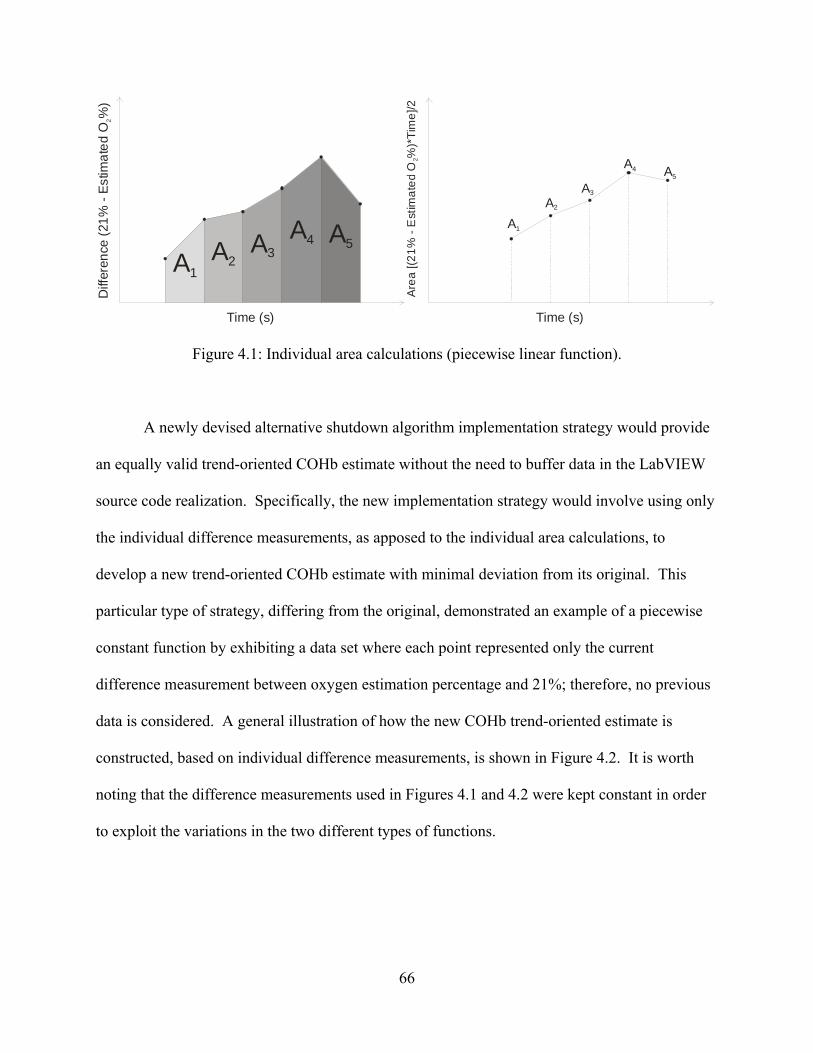
66
A5
A1A2
A3
A4
Diff
eren
ce (
21%
- E
stim
ate
d O
%)
2
Time (s)
Are
a [(
21
% -
Est
ima
ted
O%
)*T
ime
]/22
A5
A1
A2
A3
A4
Time (s)
Figure 4.1: Individual area calculations (piecewise linear function).
A newly devised alternative shutdown algorithm implementation strategy would provide
an equally valid trend-oriented COHb estimate without the need to buffer data in the LabVIEW
source code realization. Specifically, the new implementation strategy would involve using only
the individual difference measurements, as apposed to the individual area calculations, to
develop a new trend-oriented COHb estimate with minimal deviation from its original. This
particular type of strategy, differing from the original, demonstrated an example of a piecewise
constant function by exhibiting a data set where each point represented only the current
difference measurement between oxygen estimation percentage and 21%; therefore, no previous
data is considered. A general illustration of how the new COHb trend-oriented estimate is
constructed, based on individual difference measurements, is shown in Figure 4.2. It is worth
noting that the difference measurements used in Figures 4.1 and 4.2 were kept constant in order
to exploit the variations in the two different types of functions.

67
Diff
eren
ce (
21%
- E
stim
ate
d O
%)
2
Time (s) Figure 4.2: Individual difference measurements (piecewise constant function).
In order to begin such a transformation, the general COHb estimate equation in (3.8) was
revised to include the individual difference measurements (di), instead of individual area
measurements, and new heuristically developed constant coefficients were established to
compensate for the change in strategy. The newly developed trend-oriented COHb estimate
equation is shown in Equation 4.3.
43.214.6)(% inew dCOHb (4.3)
Because of the fact that the new constant coefficients in (4.3) were developed heuristically, it
was of particular interest to approximately verify, through mathematical representation, that the
change in strategy did, in fact, render an equally valid method for producing a trend-oriented
COHb estimate. First, the original trend-oriented COHb estimate from (3.9) was revisited in
Equation 4.4 and a general equation representing the new trend-oriented COHb estimate in (4.3)
was defined, as shown in Equation 4.5.
45.272.10)(% iorig ACOHb (4.4)

68
newnewkkdCOHb inew 43)(% (4.5)
In order to approximately verify the coefficients for a new trend-oriented COHb estimate based
on individual difference measurements, the individual area calculation for trapezoidal integration
in (3.7) is substituted into the original estimate in (4.4), and then subsequently approximated to
the new estimate in (4.5), as shown in Equation 4.6.
newnew
kkdttdtd
ielap
43)(45.272.102
*)1()(
(4.6)
Because the resulting equation in (4.6) consisted of two unknown coefficients and the
heuristically developed new k4 of 2.43 in (4.5) was comparable to its counterpart value of 2.45 in
(4.4), a reduced approximation equation was achieved by subtracting each value from both sides
of the equation, as shown in Equation 4.7.
new
kdttdtd
ielap
3)(72.102
*)1()(
(4.7)
Additional assumptions must be made in order to complete the approximate mathematical
verification of the new trend-oriented COHb model. Because such a large amount of data was
sampled by the ECU during NIST tests, data files were truncated by eliminating 9 data points
between computations [7]. Through observation, it was determined that this truncation led to a
sampling rate which allowed telap to be equal to approximately 0.5 s. Furthermore, it was
determined that, because samples were taken so often, even after skipping 9 data points, the
change between the current difference measurement d(t) and previous difference measurement
d(t-1) was minimal; therefore, the assumption was made that, from point-to-point, the two
difference measurements in (4.7) were approximately equal. Using this fact to combine the two
difference measurements in (4.7) into one individual difference measurement, multiplied by two,
69
along with the previous approximation of telap=0.5 s, a reduced equation was obtained, as shown
in Equation 4.8.
newkd
di
i3)(72.10
2
(4.8)
Finally, each side of the equation in (4.8) can be divided by di, which yields the fact that, in order
for the new strategy of using only individual difference measurements to create an equally valid
trend-oriented COHb estimate, the new k3 coefficient must be approximately equal to 10.72 (the
original k3 coefficient) divided by 2, or 5.36. Because of the fact that the new k3 had already
been heuristically developed to be 6.14, which is comparable to that of the theoretically produced
5.36, the approximate mathematical validation was deemed successful. It is worth noting that
the previously described Figure 4.2 is only a general representation of the newly devised
implementation strategy by way of using difference measurements, with no consideration of
changing the constant coefficients necessary in achieving a similar function as in Figure 4.1;
however, it was verified by inspection, in addition to the approximate mathematical validation,
that the two trend-oriented COHb estimates were, in fact, equally valid implementation methods.
By slightly altering the shutdown algorithm implementation strategy, appropriate modifications
to the ECU LabVIEW source code must be considered. The new shutdown algorithm
realization, which proved equally valid in producing a trend-oriented COHb estimate, eliminated
the need for data buffering, and allowed for ease of implementation is illustrated in the pseudo
code below:

70
‐Oxygen Estimation O2_calc = (Base Pulse Width / Final Pulse Width / Charge Air Temp.)*k1+k2 k1=201.55, k2=16.96 ‐Calculating Individual Difference Measurements under 21% Oxygen Threshold If CLC activated and O2_calc < 21%: Individual Difference = 21‐Current O2_calc If O2_calc > 21%:
Individual Difference = 0 ‐COHb Estimation & Shutdown Decision COHb_calc = (Individual Difference)*k3+k4, k3=6.14, k4=2.43 If COHb_calc > 10%:
total_time counter starts If COHb_calc > 10% for less than 20 seconds:
total_time counter reset to zero If COHb_calc > 10% constantly (total_time >20 seconds):
Generator shutdown triggered
4.3 Final Implementation of Shutdown Algorithm
Once all necessary revisions had been made to the shutdown algorithm realization
strategy, final implementation in the ECU could commence. Because the oxygen estimation and
shutdown algorithm were initially developed in the MATLAB software environment, they must
be implemented using LabVIEW due to the nature of the ECU’s source code. Specifically, the
oxygen estimation and shutdown algorithms were implemented into a port fuel control subVI
within the ECU source code. The decision was made to implement these algorithms in the fuel
control portion of the ECU source code in order to establish a means for terminating engine
operation if the Boolean shutdown signal was ever true. In particular, it was determined that the
most efficient method for terminating engine operation was disabling the fuel injector to ensure
that excess fuel is not unnecessarily used; therefore, upon the detection of a true Boolean
shutdown signal, appropriate LabVIEW code commands were used to disable the fuel injector.
The final ECU implementation of the oxygen estimation algorithm and shutdown algorithm,

71
based on a trend-oriented COHb estimate, in LabVIEW code are shown in Figure 4.3 and Figure
4.4, respectively. However, it is worth noting that both algorithms possess the ability to be
altered, if necessary, based on post-processing of final physical test results.
CATFiltered
Figure 4.3: LabVIEW implementation of oxygen estimation algorithm in ECU.
Filtered Oxygen Estimate
Time (s)
Figure 4.4: LabVIEW implementation of shutdown algorithm in ECU.

72
CHAPTER 5
Shutdown Algorithm Testing
For purposes of validating the newly devised oxygen depletion shutdown algorithm, a
series of indoor and outdoor tests would be conducted on the UA campus. The testing setup
included the EMS equipped generator described in Chapter 2, a selectable load bank, and
emissions analyzer. The individuals performing the tests and host computer, used for monitoring
tests, were positioned inside of a campus laboratory, away from any potential CO emissions, for
safety purposes. The tests were performed immediately outdoors of this particular campus
laboratory, providing immediate access if a test variable required altering or, in case of an
emergency, the situation could be addressed promptly. For purposes of performing the indoor
test scenarios, a mobile trailer with an approximate volume of 1420 cubic feet was placed
immediately outside of the campus laboratory to serve as an enclosed structure. A photograph,
shown in Figure 5.1, depicts the interior (on left) and exterior (on right) of the test trailer used to
simulate an indoor environment.

73
Figure 5.1: Trailer used for indoor operation test scenarios.
For outdoor testing scenarios, an area outside of the test trailer and campus laboratory was used.
The selectable load bank was used to tune the generator across a wide range of operating points,
for testing in both indoor and outdoor environments. From the broad spectrum of operating
modes, six particular loads were chosen for purposes of performing validation tests at UA, as
shown in Table 5.1. Because testing during this project’s previous phase, as well as tests
performed at NIST, utilized a six mode method, it was of particular interest to use the same load
points as described in [6,7] for continuity.
Table 5.1 Load points used for validation testing at UA.
Mode Load (W) 1 0 2 500 3 1500 4 3500 5 4750 6 5500
The final piece of equipment used in the setup for validation testing at UA was the emissions
analyzer. Specifically, a weatherproof Nova 376 Series portable analyzer was appropriately

74
calibrated for measuring oxygen (%) and CO (ppm) gases in the surrounding air. The analyzer
completes these measurements by way of electrochemical sensors with a resolution of 0.1%
oxygen and 1 ppm CO [12]. In order to achieve the most unbiased emissions data, with respect
to the generator’s location, the attached sampling line must be placed in a central location inside
of the test trailer. Furthermore, the generator was positioned at the far end of the test trailer,
while the emissions sampling line was positioned in the center of the test trailer. It is worth
noting that the Nova emissions analyzer was not used for outdoor testing scenarios, as the
surrounding air should experience only minimal oxygen depletion. Furthermore, it was assumed
that the emissions in the surrounding air were comprised of 21% oxygen and 0 ppm CO,
approximately that of ambient air, for outdoor tests cases. A photograph, shown in Figure 5.2,
depicts the Nova emissions analyzer used throughout indoor testing.
Figure 5.2: Nova analyzer used to measure emissions in enclosed environment.

75
In order to replicate a broad spectrum of real-life operating conditions for a gasoline
powered generator on the UA campus, several variables must be considered. Specifically, tests
were conducted in indoor and outdoor environments, under constant and cyclic load profiles, and
under random load profiles. However, all test cases included the use of a muffler catalyst due to
the fact that the generator had already been modified for low CO emissions in the previous phase
of this project. For purposes of demonstrating that the oxygen estimation and shutdown
algorithms functioned properly under constant load, a low, medium, and high load were
specifically chosen from the load points listed in Table 5.1. In addition, these same low,
medium, and high load points were used to demonstrate the validity of the algorithms under
cyclic loads by conducting a low-to-high load profile test and high-to-low load profile test.
Finally, in order to ensure that the newly developed algorithms did not produce any false-
positive shutdowns with sudden and significant load changes, random load profile tests were
conducted using all load points described in Table 5.1 for both, indoor and outdoor,
environments. Specifically, two random load profiles were generated, with each profile to be
conducted once indoors and once outdoors. The twelve testing scenarios conducted at UA are
detailed and identified, accordingly, by name, as shown in Table 5.2.

76
Table 5.2 Operating conditions used for validation testing at UA.
Test ID Load Profile Environment UA1 Constant (500 W) Indoors UA2 Constant (3000 W) Indoors UA3 Constant (5500 W) Indoors UA4 Cyclic (Low to High) Indoors UA5 Cyclic (High to Low) Indoors UA6 Random 1 (All Loads) Indoors UA7 Random 2 (All Loads) Indoors UA8 Constant (500 W) Outdoors UA9 Constant (3000 W) Outdoors UA10 Constant (5500 W) Outdoors UA11 Random 1 (All Loads) Outdoors UA12 Random 2 (All Loads) Outdoors
An effort was made to maintain a testing procedure that was as consistent as possible
throughout all of the previously described test cases. The subsequent sections highlight the
procedures used for both, indoor and outdoor, testing environments, the results of all twelve tests
conducted, and a brief description of observations and conclusions drawn from analyzing the
resulting test data.
5.1 Indoor Testing
For indoor testing, the initial step included opening both trailer doors while a large fan
was used for two reasons: 1) to blow out any emissions remaining from the previous test,
essentially cleaning the air within the trailer and returning it to approximately an ambient state,
and 2) to speed up the cooling process of the generator. The generator must be cooled back to an
ambient temperature as each of the validation test cases, performed at UA, were conducted with
a cold start. Once ambient generator temperature and air chemistry were achieved, the generator

77
was cranked and operated with open-loop control while the fan continued to blow out any
emissions not resulting from CLC. This process continued while waiting on the oxygen sensor,
used for feedback, to appropriately heat for activation. A time of approximately 30 s was usually
needed before the oxygen sensor could begin properly functioning. Upon heating of the oxygen
sensor, CLC was activated, the fan was turned off, and both trailer doors were closed, allowing
for the replication of an enclosed operating environment.
During the course of indoor testing, the ECU was used to collect relevant data, in
intervals of 0.5 s, which included the following variables: run time (s), shutdown signal
(Boolean), engine speed (RPM), oil temperature (°C), MAP (kPa), CAT (°C), base VE, final VE,
oxygen estimation (%), COHb estimation (%), measured oxygen (%), and measured CO (ppm).
The actual COHb (%) from the provided CPSC calculation was also included in the final data
files; however, these calculations were completed during data post-processing and subsequently
added to the data files. For validation purposes, it was of particular interest to plot oxygen
estimation (in green) with oxygen measured (in blue), COHb estimation (in green) with CPSC
COHb calculation (in blue), CO emissions, and the generator shutdown signal. The following
plots, shown in Figure 5.3 through Figure 5.9, which were generated through post-processing of
the resultant data in the MATLAB software environment, illustrate the results collected from all
indoor tests described in Table 5.2. Because of the large data file sizes, 9 points were skipped
between computations, similar to that done during the post-processing of NIST test data and
development of the algorithms.

78
0 200 400 600 800 1000 1200 1400 1600 180015
16
17
18
19
20
21
22
23
24
25
Time (s)
%O
2
Oxygen Estimation (0.5 kW - Indoors)
O2 meas
O2 calc
Figure 5.3(a): Oxygen estimation and oxygen measured for Test UA1.
0 200 400 600 800 1000 1200 1400 1600 18000
5
10
15
20
25
30
Time (s)
CO
Hb
%
COHb Estimation (0.5 kW - Indoors)
COHb meas (CPSC)
COHb calc
Figure 5.3(b): COHb estimation and CPSC COHb calculation for Test UA1.

79
0 200 400 600 800 1000 1200 1400 1600 18000
100
200
300
400
500
600
700
800
900
1000
Time (s)
CO
(pp
m)
CO Emissions (0.5 kW - Indoors)
CO emis
Figure 5.3(c): Measured CO emissions for Test UA1.
0 200 400 600 800 1000 1200 1400 1600 1800-1
-0.5
0
0.5
1
1.5
2
Time (s)
Shu
tdow
n S
igna
l (B
oole
an)
Shutdown Signal (0.5 kW - Indoors)
Shutdown Signal
Figure 5.3(d): Algorithm shutdown signal for Test UA1.
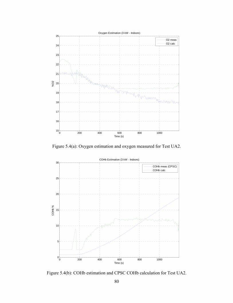
80
0 200 400 600 800 100015
16
17
18
19
20
21
22
23
24
25
Time (s)
%O
2
Oxygen Estimation (3 kW - Indoors)
O2 meas
O2 calc
Figure 5.4(a): Oxygen estimation and oxygen measured for Test UA2.
0 200 400 600 800 10000
5
10
15
20
25
30
Time (s)
CO
Hb
%
COHb Estimation (3 kW - Indoors)
COHb meas (CPSC)
COHb calc
Figure 5.4(b): COHb estimation and CPSC COHb calculation for Test UA2.

81
0 200 400 600 800 10000
200
400
600
800
1000
1200
1400
1600
1800
2000
Time (s)
CO
(pp
m)
CO Emissions (3 kW - Indoors)
CO emis
Figure 5.4(c): Measured CO emissions for Test UA2.
0 200 400 600 800 1000-1
-0.5
0
0.5
1
1.5
2
Time (s)
Shu
tdow
n S
igna
l (B
oole
an)
Shutdown Signal (3 kW - Indoors)
Shutdown Signal
Figure 5.4(d): Algorithm shutdown signal for Test UA2.

82
0 500 1000 150015
16
17
18
19
20
21
22
23
24
25
Time (s)
%O
2
Oxygen Estimation (5.5 kW - Indoors)
O2 meas
O2 calc
Figure 5.5(a): Oxygen estimation and oxygen measured for Test UA3.
0 500 1000 15000
5
10
15
20
25
30
Time (s)
CO
Hb
%
COHb Estimation (5.5 kW - Indoors)
COHb meas (CPSC)
COHb calc
Figure 5.5(b): COHb estimation and CPSC COHb calculation for Test UA3.

83
0 500 1000 15000
200
400
600
800
1000
1200
1400
1600
1800
2000
Time (s)
CO
(pp
m)
CO Emissions (5.5 kW - Indoors)
CO emis
Figure 5.5(c): Measured CO emissions for Test UA3.
0 500 1000 1500-1
-0.5
0
0.5
1
1.5
2
Time (s)
Shu
tdow
n S
igna
l (B
oole
an)
Shutdown Signal (5.5 kW - Indoors)
Shutdown Signal
Figure 5.5(d): Algorithm shutdown signal for Test UA3.

84
0 200 400 600 800 1000 120015
16
17
18
19
20
21
22
23
24
25
Time (s)
%O
2
Oxygen Estimation (Cyclic Load: Low to High - Indoors)
O2 meas
O2 calc
Figure 5.6(a): Oxygen estimation and oxygen measured for Test UA4.
0 200 400 600 800 1000 12000
5
10
15
20
25
30
Time (s)
CO
Hb
%
COHb Estimation (Cyclic Load: Low to High - Indoors)
COHb meas (CPSC)
COHb calc
Figure 5.6(b): COHb estimation and CPSC COHb calculation for Test UA4.

85
0 200 400 600 800 1000 12000
500
1000
1500
Time (s)
CO
(pp
m)
CO Emissions (Cyclic Load: Low to High - Indoors)
CO emis
Figure 5.6(c): Measured CO emissions for Test UA4.
0 200 400 600 800 1000 1200-1
-0.5
0
0.5
1
1.5
2
Time (s)
Shu
tdow
n S
igna
l (B
oole
an)
Shutdown Signal (Cyclic Load: Low to High - Indoors)
Shutdown Signal
Figure 5.6(d): Algorithm shutdown signal for Test UA4.

86
0 200 400 600 800 1000 1200 1400 160015
16
17
18
19
20
21
22
23
24
25
Time (s)
%O
2
Oxygen Estimation (Cyclic Load: High to Low - Indoors)
O2 meas
O2 calc
Figure 5.7(a): Oxygen estimation and oxygen measured for Test UA5.
0 200 400 600 800 1000 1200 1400 16000
5
10
15
20
25
30
Time (s)
CO
Hb
%
COHb Estimation (Cyclic Load: High to Low - Indoors)
COHb meas (CPSC)
COHb calc
Figure 5.7(b): COHb estimation and CPSC COHb calculation for Test UA5.

87
0 200 400 600 800 1000 1200 1400 16000
200
400
600
800
1000
1200
1400
1600
1800
2000
Time (s)
CO
(pp
m)
CO Emissions (Cyclic Load: High to Low - Indoors)
CO emis
Figure 5.7(c): Measured CO emissions for Test UA5.
0 200 400 600 800 1000 1200 1400 1600-1
-0.5
0
0.5
1
1.5
2
Time (s)
Shu
tdow
n S
igna
l (B
oole
an)
Shutdown Signal (Cyclic Load: High to Low - Indoors)
Shutdown Signal
Figure 5.7(d): Algorithm shutdown signal for Test UA5.

88
0 200 400 600 800 1000 1200 1400 1600 180015
16
17
18
19
20
21
22
23
24
25
Time (s)
%O
2
Oxygen Estimation (Random Load Profile 1 - Indoors)
O2 meas
O2 calc
Figure 5.8(a): Oxygen estimation and oxygen measured for Test UA6.
0 200 400 600 800 1000 1200 1400 1600 18000
2
4
6
8
10
12
14
16
18
20
Time (s)
CO
Hb
%
COHb Estimation (Random Load Profile 1 - Indoors)
COHb meas (CPSC)
COHb calc
Figure 5.8(b): COHb estimation and CPSC COHb calculation for Test UA6.

89
0 200 400 600 800 1000 1200 1400 1600 18000
50
100
150
200
250
300
350
400
450
500
Time (s)
CO
(pp
m)
CO Emissions (Random Load Profile 1 - Indoors)
CO emis
Figure 5.8(c): Measured CO emissions for Test UA6.
0 200 400 600 800 1000 1200 1400 1600 1800-1
-0.5
0
0.5
1
1.5
2
Time (s)
Shu
tdow
n S
igna
l (B
oole
an)
Shutdown Signal (Random Load Profile 1 - Indoors)
Shutdown Signal
Figure 5.8(d): Algorithm shutdown signal for Test UA6.
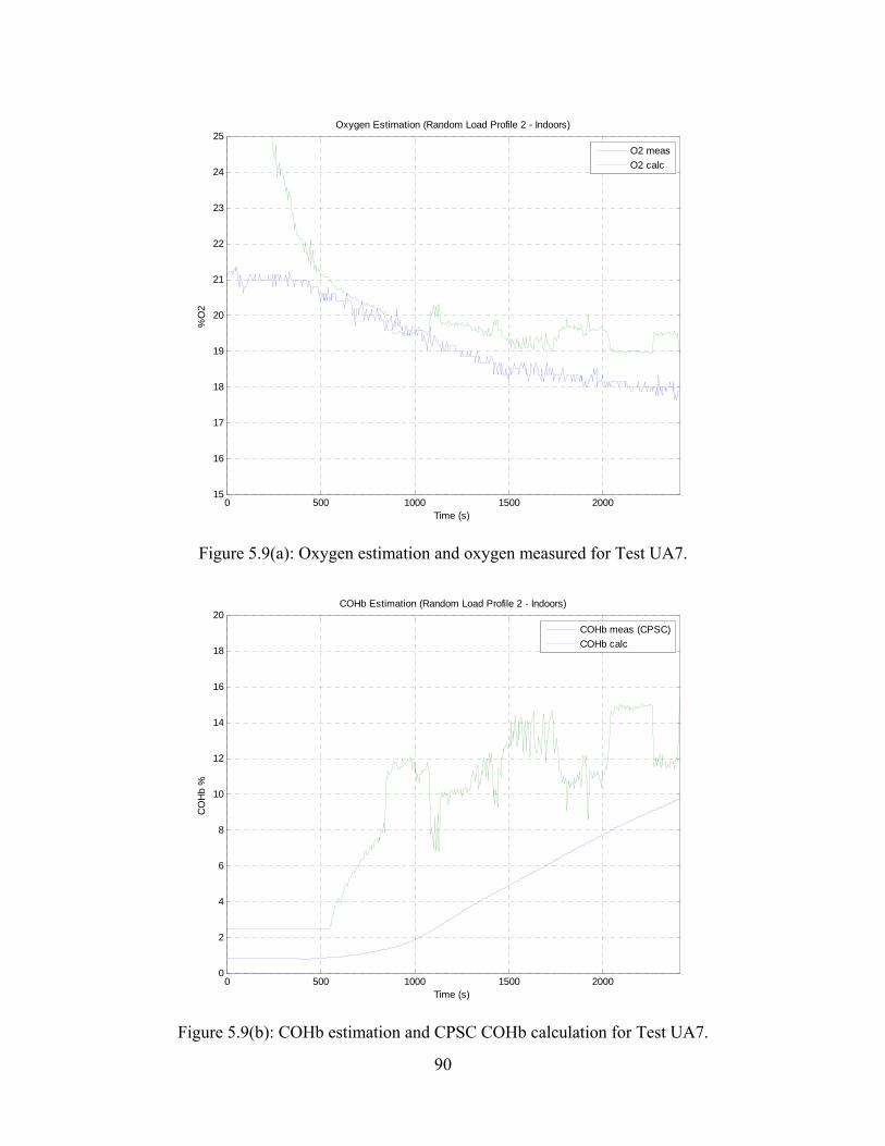
90
0 500 1000 1500 200015
16
17
18
19
20
21
22
23
24
25
Time (s)
%O
2
Oxygen Estimation (Random Load Profile 2 - Indoors)
O2 meas
O2 calc
Figure 5.9(a): Oxygen estimation and oxygen measured for Test UA7.
0 500 1000 1500 20000
2
4
6
8
10
12
14
16
18
20
Time (s)
CO
Hb
%
COHb Estimation (Random Load Profile 2 - Indoors)
COHb meas (CPSC)
COHb calc
Figure 5.9(b): COHb estimation and CPSC COHb calculation for Test UA7.

91
0 500 1000 1500 20000
100
200
300
400
500
600
Time (s)
CO
(pp
m)
CO Emissions (Random Load Profile 2 - Indoors)
CO emis
Figure 5.9(c): Measured CO emissions for Test UA7.
0 500 1000 1500 2000-1
-0.5
0
0.5
1
1.5
2
Time (s)
Shu
tdow
n S
igna
l (B
oole
an)
Shutdown Signal (Random Load Profile 2 - Indoors)
Shutdown Signal
Figure 5.9(d): Algorithm shutdown signal for Test UA7.

92
5.2 Outdoor Testing
Although similar to that of indoor testing, the procedure used for outdoor testing was
much simpler and involved fewer steps. The initial step still involved using the fan to speed the
generator’s cooling process. Once an ambient generator temperature was achieved, the fan’s
operation was terminated and the generator was cranked for a cold start. Because the generator
did not reach such high temperatures, as experienced during indoor testing, the cool down time
was significantly reduced. Similar to the indoor testing procedure, the generator was operated in
an open-loop manner until the oxygen sensor heated. Once the oxygen sensor was heated, after
about 30 s, CLC was activated and an outdoor test environment replication was complete.
During the course of outdoor testing, the ECU was once again used to collect relevant
data, in intervals of 0.5 s, which included the same variables recorded for indoor testing;
however, measured oxygen and CO were not recorded, as previously mentioned, and
approximate ambient air conditions were assumed. Specifically, measured oxygen was assumed
to be 21% and measured CO was assumed to be 0 ppm. Because of this assumption, the CPSC
calculation resulted in approximately 1% COHb, due to its dependency on CO, when given the
input of 0 ppm CO; therefore, the actual COHb, as calculated using the method provided by
CPSC, was assumed to be 1% for all outdoor test results. It is worth noting that this same basis
for CPSC COHb calculation was used in the shutdown algorithm development stage. For
validation of outdoor test cases, it was of particular interest to plot oxygen estimation (in green)
with assumed oxygen measured (in blue) and COHb estimation (in green) with assumed CPSC
COHb calculation (in blue). The Boolean shutdown signal was not plotted because the algorithm
did not trigger a shutoff when tested outdoors. The following plots, shown in Figure 5.10
through Figure 5.14, which were generated through post-processing of the resultant data in the

93
MATLAB software environment, illustrate the results collected from all outdoor tests described
in Table 5.2. As was the case for indoor test plots, 9 points were skipped between computations
because of the large data file sizes, similar to that done during the post-processing of NIST test
data and algorithm developments.
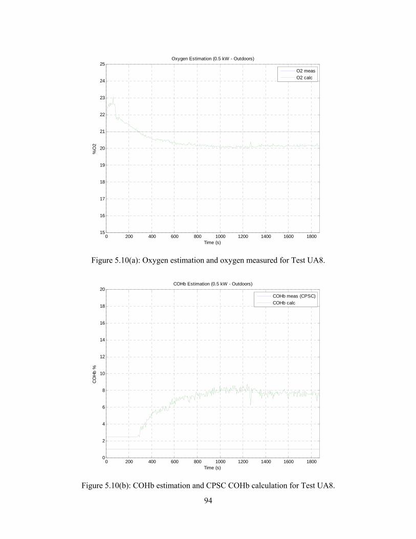
94
0 200 400 600 800 1000 1200 1400 1600 180015
16
17
18
19
20
21
22
23
24
25
Time (s)
%O
2
Oxygen Estimation (0.5 kW - Outdoors)
O2 meas
O2 calc
Figure 5.10(a): Oxygen estimation and oxygen measured for Test UA8.
0 200 400 600 800 1000 1200 1400 1600 18000
2
4
6
8
10
12
14
16
18
20
Time (s)
CO
Hb
%
COHb Estimation (0.5 kW - Outdoors)
COHb meas (CPSC)
COHb calc
Figure 5.10(b): COHb estimation and CPSC COHb calculation for Test UA8.
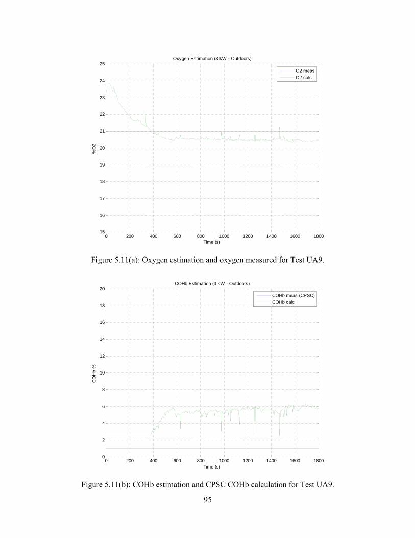
95
0 200 400 600 800 1000 1200 1400 1600 180015
16
17
18
19
20
21
22
23
24
25
Time (s)
%O
2
Oxygen Estimation (3 kW - Outdoors)
O2 meas
O2 calc
Figure 5.11(a): Oxygen estimation and oxygen measured for Test UA9.
0 200 400 600 800 1000 1200 1400 1600 18000
2
4
6
8
10
12
14
16
18
20
Time (s)
CO
Hb
%
COHb Estimation (3 kW - Outdoors)
COHb meas (CPSC)
COHb calc
Figure 5.11(b): COHb estimation and CPSC COHb calculation for Test UA9.

96
0 200 400 600 800 1000 1200 1400 1600 180015
16
17
18
19
20
21
22
23
24
25
Time (s)
%O
2
Oxygen Estimation (5.5 kW - Outdoors)
O2 meas
O2 calc
Figure 5.12(a): Oxygen estimation and oxygen measured for Test UA10.
0 200 400 600 800 1000 1200 1400 1600 18000
2
4
6
8
10
12
14
16
18
20
Time (s)
CO
Hb
%
COHb Estimation (5.5 kW - Outdoors)
COHb meas (CPSC)
COHb calc
Figure 5.12(b): COHb estimation and CPSC COHb calculation for Test UA10.

97
0 500 1000 1500 2000 2500 3000 350015
16
17
18
19
20
21
22
23
24
25
Time (s)
%O
2
Oxygen Estimation (Random Load Profile 1 - Outdoors)
O2 meas
O2 calc
Figure 5.13(a): Oxygen estimation and oxygen measured for Test UA11.
0 500 1000 1500 2000 2500 3000 35000
2
4
6
8
10
12
14
16
18
20
Time (s)
CO
Hb
%
COHb Estimation (Random Load Profile 1 - Outdoors)
COHb meas (CPSC)
COHb calc
Figure 5.13(b): COHb estimation and CPSC COHb calculation for Test UA11.

98
0 500 1000 1500 2000 2500 3000 350015
16
17
18
19
20
21
22
23
24
25
Time (s)
%O
2
Oxygen Estimation (Random Load Profile 2 - Outdoors)
O2 meas
O2 calc
Figure 5.14(a): Oxygen estimation and oxygen measured for Test UA12.
0 500 1000 1500 2000 2500 3000 35000
2
4
6
8
10
12
14
16
18
20
Time (s)
CO
Hb
%
COHb Estimation (Random Load Profile 2 - Outdoors)
COHb meas (CPSC)
COHb calc
Figure 5.14(b): COHb estimation and CPSC COHb calculation for Test UA12.

99
5.3 Analysis and Discussion of Validation Test Results
It is worth noting that test data continued to record, even past the point where a true
shutdown signal was detected. Although it was verified that the generator would, in fact,
shutdown upon detection of a true Boolean shutdown signal by disabling the fuel injector, the
generator was allowed to continue running well past the signaled termination point in order to
collect a sufficient amount of data. It was observed that the temperature normally increased
when an enclosed environment was detected and when higher loads were experienced. For all
cases, the test duration was predetermined to allow for capturing an adequate quantity of data;
however, all indoor tests except that of UA1 required an early termination, due to a critically
high oil temperature, in order to prevent any potential generator damage. Alternatively, all
outdoor tests were able to successfully run for their predetermined duration because the oil
temperature did not rise to a critically high level.
Several important observations were made through post-processing and analysis of the
resulting validation test data. By inspection of the resulting oxygen data, it was determined that
the oxygen estimation algorithm normally displayed a minimal overestimate of measured oxygen
in indoor tests and minimal underestimate of measured oxygen in the outdoor tests. However,
some overestimations and underestimations were expected due to the curve fitting method
employed during the development stage, which considered a wide range of operating scenarios.
In order for the algorithm to estimate oxygen content as accurately as possible, for a broad
spectrum of real-life operating conditions, sacrifices must be made to compensate for the large
variations experienced between indoor and outdoor test conditions. Nonetheless, the outdoor
tests should not underestimate oxygen to the extent of producing a false-positive shutdown and
the indoor tests should not overestimate oxygen to the extent of allowing the generator to run too

100
far past the ideal termination point; therefore, the oxygen estimation algorithm development was
deemed to be a success. With respect to the shutdown decision, it was observed that all COHb
estimations increased quicker than that of the CPSC COHb calculation which led to an earlier
shutdown time than originally expected; however, this was determined to be more efficient than
the alternative of shutting down later than expected because of the dangerous environments
experienced if such a situation arose. It can also be observed from several tests, particularly in
Tests UA2, UA3, and UA5, that the CO emissions tended to level out at approximately 1700
ppm. This phenomenon was believed to be caused by saturation.
In summary, the algorithm produced an oxygen estimation, as anticipated from the
development phase, across a broad range of range of real-life operating scenarios. When higher
levels of CO were experienced, as expected when operating in an enclosed structure, the
algorithm subsequently signaled an oxygen depleted environment and shutdown the engine
based on a trend oriented COHb estimate. Also, the oxygen depletion shutdown algorithm
proved successful when operating in an outdoor environment by not producing any false-positive
shutdowns. Furthermore, the random load profile tests demonstrated that the algorithm would
not produce any nuisance shutdowns when subjected to sudden and significant load changes.
Based on these significant observations which prove that the generator operation will be
terminated by the time hazardous conditions are reached, along with the fact that no false-
positive shutdowns are produced outdoors, the oxygen depletion shutdown algorithm was
deemed to be valid. The results of all tests which should produce a generator shutdown (all
indoor tests) are summarized in Table 5.3, where (SD) represents shutdown. These results
provide a validation of the shutdown algorithm by detailing the COHb estimate, CPSC COHb
calculation, measured CO emissions, and estimated oxygen at the algorithm shutdown time and

101
ideal shutdown time (10% CPSC COHb for constant 20 s). Due to the fact that CPSC COHb
calculation did not reach 10% in all of the tests, due to a critically high oil temperature, some
cells are labeled as not applicable (NA); however, 10% CPSC COHb would have been achieved
if these particular tests would have been allowed to continue. Finally, although the ECU allowed
for source code alterations, it was decided that no modifications to the oxygen depletion
shutdown algorithm were necessary following post-processing of validation test data.
Table 5.3 Summary of validation testing results at UA.
Test
Actual SD
Time (s)
Ideal CPSC
SD Time
(s)
COHb Est.
(%) at SD
COHb CPSC (%) at
SD
COHb Est.
(%) at Ideal SD
COHb CPSC (%) at Ideal SD
CO (ppm) at SD
CO (ppm)
at Ideal SD
O2 Est. (%)
at SD
O2 Est. (%) at
Ideal SD
UA1 591 NA 10.47 1.34 NA NA 227 NA 19.69 NA
UA2 526 782 10.81 5.24 12.39 10.43 1313 1700 19.64 19.38
UA3 484 899 11.03 3.64 14.73 10.44 907 1696 19.60 19.00
UA4 873 NA 12.06 2.27 NA NA 496 NA 19.43 NA
UA5 687 1100 10.39 2.69 11.70 10.43 730 1693 19.70 19.49
UA6 770 NA 10.53 1.18 NA NA 109 NA 19.68 NA
UA7 870 NA 11.12 1.40 NA NA 220 NA 19.59 NA

102
CHAPTER 6
Conclusions
This thesis has described the process and components used to develop a more reliable
safety shutdown feature for a gasoline powered generator already modified for low CO
emissions. An EMS equipped Coleman Powermate 7000, similar to the configuration in this
project's previous phase, was utilized for engine operation and control to achieve a
stoichiometric fuel mixture, 14.6 to 1 AFR. For purposes of implementing a new shutdown
algorithm, an advantageous Drivven based ECU was acquired to serve as a replacement to the
existing Delphi based ECU. The new safety shutdown feature was dependent upon an oxygen
estimation algorithm executed without the use of any emissions sensors. Oxygen estimation was
developed heuristically by post-processing NIST test data and improved by employing a curve
fitting method across a broad operating spectrum.
Once an enhanced oxygen estimation algorithm was developed, it was then used to
establish a trend oriented COHb estimate which provided a basis for a shutdown decision.
Simulations were performed with the newly developed oxygen depletion shutdown algorithm,
using data from previous NIST tests, for purposes of off-line verification. Off-line simulations
resulted in an algorithm which would trigger a shutoff when operating in an oxygen depleted
environment and prevent false-positive shutdowns in outdoor environment. The algorithm was
implemented into the Drivven ECU, which allowed for modifications and additions to its source

103
code, unlike its predecessor. Finally, a series of validation tests, which represented a wide range
of real-life operating conditions, were conducted at UA to ensure that the shutdown algorithm
worked as expected. Upon analysis and post-processing of validation test results, it was
determined that the shutdown algorithm produced a shutoff when operating in an enclosed
environment and did not nuisance trip when operating outdoors; therefore, no further
modifications were made to the oxygen depletion shutdown algorithm as it was deemed
successful.
6.1 Future Work
Due to the large size of the Drivven based ECU, it cannot be mounted to the generator for
demonstration of a finalized product. Therefore, future work on this project will include an ECU
and oxygen depletion shutdown algorithm implementation on a deliverable platform.
Specifically, an embedded engine controller produced by MicroSquirt will be used for final
implementation through means of modifying its existing source code, in the C programming
language, to mimic that of the operation and control scheme in the Drivven based ECU. Due to
the nature of its smaller size, the MicroSquirt controller will allow for direct mounting to the
generator and completion of the final deliverable prototype to CPSC.

104
REFERENCES
[1] Consumer Product Safety Commission Website, “Carbon Monoxide Questions and Answers, CPSC Document #466”, http://www.cpsc.gov/cpscpub/pubs/466.html, 2008.
[2] Consumer Product Safety Commission Website, “Incidents, Deaths, and In-Depth
Investigations Associated with Non-Fire Carbon Monoxide from Engine-Driven Generators and Other Engine-Driven Tools, 1999-2010”, http://www.cpsc.gov/library/coed11.pdf, 2011.
[3] Environmental Protection Agency Website, “Air Quality Criteria for Carbon Monoxide”,
http://www.epa.gov/ncea/pdfs/coaqcd.pdf, 2000. [4] Drivven Website, http://www.drivven.com/, n.d., Accessed on: October 12, 2012. [5] National Instruments Website, “NI cRIO-9022”, http://sine.ni.com/ds/app/doc/p/id/ds-
202/lang/en, 2012. [6] Smelser, Jennifer Beasley, “Oxygen Depletion Shutdown Algorithm for Portable
Gasoline Generators”, MS Thesis, The University of Alabama, 2009. [7] Tim A. Haskew, Paul Puzinauskas, “Algorithm Development for Enclosed Operation
Detection and Shutoff of a Portable Gasoline-Powered Generator”, Final Project Report, 2011.
[8] William B. Ribbins, Understanding Automotive Electronics, Butterworth-Heinemann,
Fifth Edition, 1998. [9] Delphi Website, “Delphi MT05 Engine Control Module Series”,
http://delphi.com/shared/pdf/ppd/pwrtrn/mt05.pdf, 2007. [10] Mathworks Website, http://www.mathworks.com/products/matlab/, 2012. [11] National Instruments Website, http://www.ni.com/labview/, 2012. [12] Nova Analytical Systems Website, “Item # Model 376WP”, http://catalog.nova-
gas.com/item/carbon-monoxide-co-/dioxide-and-oxides-of-nitrogen-analyzer-376-series/series-376?&plpver=10&origin=keyword&by=prod&filter=0, 2010.

105
APPENDIX
Oxygen Depletion Shutdown Algorithm Code used for Off-Line Validations
%Oxygen Depletion Algorithm (refinements) %This code uses multi-raw data files for O2 estimation %CPSC - University of Alabama nwin=1024; nfiles=input('enter number of MT05 files '); nskip=input('enter number of lines to skip '); for p=1:nfiles; p fname=input('enter MT05 path and filename ','s'); indat1=fopen(fname); Odat=fscanf(indat1,'%e',inf); junkn=int32(size(Odat)/43) ndata=junkn(1) %Gather input data tag=0; linecnt=0; for i=1:43:(ndata-1)*43+1; tag=tag+1; if(Odat(i+6)<100); linecnt=tag; else; break; end; end; linecnt=linecnt+1 tbase=Odat(43*linecnt)/1000; k=0; for i=(linecnt-1)*43+1:43*(nskip+1):((ndata-1)*43+1); k=k+1; tsim(p,k)=Odat(i+42)/1000-tbase; VRPM(p,k)=Odat(i+6); VCLTS(p,k)=Odat(i+9); VIAT(p,k)=Odat(i+10); MAP(p,k)=Odat(i+11); CAT(p,k)=Odat(i+19); PW(p,k)=Odat(i+20); BPW(p,k)=Odat(i+21); CLC(p,k)=Odat(i+23); end; cnt(p)=k; end;

106
%Final O2 estimation equation O2calc=(BPW./PW./CAT)*201.55+16.96; clear Odat; %Gather emissions data assuming 1 second intervals ename=input('enter NIST path and filename ','s'); indat2=fopen(ename); Edatin=fscanf(indat2,'%e',inf); junke=int32(size(Edatin)/3); edata=junke(1) k=0; %Input emissions on 6 second intervals for i=1:3:((edata-1)*3+1); k=k+1; temis(k)=(k-1)*60*6; O2emis(k)=Edatin(i+0); COemis(k)=Edatin(i+1); COHb(k)=Edatin(i+2); end; clear Edatin; for i=2:nfiles tsim(i,:)=tsim(i,:)+tsim(i-1,cnt(i-1)); end; k=0; for i=1:nfiles for m=1:cnt(i); k=k+1; tcal(k)=tsim(i,m); O2longraw(k)=O2calc(i,m); VRPMlongraw(k)=VRPM(i,m); MAPlongraw(k)=MAP(i,m); CATlongraw(k)=CAT(i,m); PWlongraw(k)=PW(i,m); BPWlongraw(k)=BPW(i,m); VCLTSlongraw(k)=VCLTS(i,m); VIATlongraw(k)=VIAT(i,m); end; end; %tmax=tcal(k); dlength=k-1; tmax=max(tcal); O2long=filter(ones(1,nwin)/nwin,1,O2longraw); MAPlong=filter(ones(1,nwin)/nwin,1,MAPlongraw); VCLTSlong=filter(ones(1,nwin)/nwin,1,VCLTSlongraw); VIATlong=filter(ones(1,nwin)/nwin,1,VIATlongraw); PWlong=filter(ones(1,nwin)/nwin,1,PWlongraw); BPWlong=filter(ones(1,nwin)/nwin,1,BPWlongraw); %Redefine CAT with new lookup table - Information proprietary to Delphi %Redefine O2longraw & O2long, based on new CAT factor table O2longraw=(BPWlongraw./PWlongraw./CATfilt3)*201.55+16.96; %Use for Test U %O2longraw=(BPWlongraw./PWlongraw./CATlongraw3)*201.55+16.96; O2long=filter(ones(1,nwin)/nwin,1,O2longraw);

107
total_area_filt=0; total_area_raw=0; flag_filt=1; flag_raw=1; shutdown_flag_filt=0; shutdown_flag_raw=0; O2_threshold=21 peak_filt=max(O2long); peak_raw=max(O2longraw); [m,n]=size(tcal); for w=1:n if O2long(w)==peak_filt cell_filt=w; end; if O2longraw(w)==peak_raw cell_raw=w; end; O2_threshold_vector(w)=O2_threshold; end; for x=1:n if x>(cell_filt-1) if O2_threshold-O2long(x)>0; diff_filt(flag_filt)=O2_threshold-O2long(x); diff_filt_sq(flag_filt)=diff_filt(flag_filt)*diff_filt(flag_filt); if flag_filt>1 h=tcal(x)-tcal(x-1); integral_area=h*(diff_filt(flag_filt-1)+diff_filt(flag_filt))/2; %Use for individual area strategy ia_filt(x)=h*(diff_filt(flag_filt-1)+diff_filt(flag_filt))/2; %Use for individual difference strategy %ia_filt(x)=diff_filt(flag_filt); ia_filt_sq(x)=h*(diff_filt_sq(flag_filt-1)+diff_filt_sq(flag_filt))/2; total_area_filt(x)=total_area_filt(x-1)+ia_filt(x); else total_area_filt(x)=0; ia_filt(x)=0; end; flag_filt=flag_filt+1; else if flag_filt>2 total_area_filt(x)=total_area_filt(x-1); else total_area_filt(x)=0; end; ia_filt(x)=0; end; else total_area_filt(x)=0; ia_filt(x)=0; end;

108
if x>(cell_raw-1) if O2_threshold-O2longraw(x)>0; diff_raw(flag_raw)=O2_threshold-O2longraw(x); diff_raw_sq(flag_raw)=diff_raw(flag_raw)+diff_raw(flag_raw); if flag_raw>1 h=tcal(x)-tcal(x-1); integral_area=h*(diff_raw(flag_raw-1)+diff_raw(flag_raw))/2; ia_raw(x)=h*(diff_raw_sq(flag_raw-1)+diff_raw_sq(flag_raw))/2; total_area_raw(x)=total_area_raw(x-1)+integral_area; else total_area_raw(x)=0; ia_raw(x)=0; end; flag_raw=flag_raw+1; else if flag_raw>2 total_area_raw(x)=total_area_raw(x-1); else total_area_raw(x)=0; end; ia_raw(x)=0; end; else total_area_raw(x)=0; ia_raw(x)=0; end; end; tot_area_filt=total_area_filt(end); tot_area_raw=total_area_raw(end); %Used for ind. area COHbcalc=(ia_filt)*10.72+2.45; %Used for ind. diff %COHbcalc=(ia_filt)*6.14+2.43; COHblongraw=COHbcalc; COHblong=filter(ones(1,nwin)/nwin,1,COHblongraw); SDflag=0; start_flag=0; t_total=0; for x=200:(n-200) if COHblong(x)>9.999 if SDflag==0; if start_flag==0; t_start=tcal(x); start_flag=1; else t_total=tcal(x)-t_start; end; if t_total>19.999 SDflag=1; disp('Generator Shutdown @ time: ') tcal(x) disp('COHb Estimate: ') COHblong(x)

109
disp('Total Area (Filtered): ') total_area_filt(x) disp('O2 Estimate: ') O2long(x) end; end; else start_flag=0; end; end; if SDflag==0 disp('Generator did NOT shutdown!') end; figure plot(temis,COHb,tcal,COHblong) xlabel('Time (s)') ylabel('COHb %') legend('est','filt orig') title('COHb estimates') axis([0 tmax 0 80]) grid ON figure [AX,H1,H2]=plotyy(temis,O2emis,temis,COHb) hold on plot(AX(1),tcal,O2long,'red') hold off set(get(AX(1),'ylabel'),'String','%O2') set(get(AX(2),'ylabel'),'String','Predicted %COHb') xlim(AX(1),[0 tmax]) xlim(AX(2),[0 tmax]) ylim(AX(1),[15 25]) ylim(AX(2),[0 20]) set(AX(1),'ytick',15:25) set(AX(2),'ytick',0:2:20) xlabel('Time (s)') legend('O2 emis','O2 calc filt','COHb') grid ON figure subplot(3,1,1) [AX,H1,H2]=plotyy(temis,COemis,temis,COHb) legend('CO emis','COHb') set(get(AX(1),'ylabel'),'String','Measured CO (ppm)') set(get(AX(2),'ylabel'),'String','Predicted %COHb') xlim(AX(1),[0 tmax]) xlim(AX(2),[0 tmax]) ylim(AX(1),[0 500]) ylim(AX(2),[0 20]) set(AX(1),'ytick',0:100:500) set(AX(2),'ytick',0:4:20) xlabel('Time (s)') grid ON subplot(3,1,2)

110
plot(tcal,ia_filt) xlabel('Time(s)') ylabel('Individual Area') title('Individual Area Measurements under O2 threshold (using filt line)') axis([0 tmax 0 2]) grid ON subplot(3,1,3) plot(tcal,total_area_filt) xlabel('Time(s)') ylabel('Total Area') title('Total Area under O2 threshold (using filt line)') axis([0 tmax 0 tot_area_filt]) grid ON