1

Modeling Bimodal Discrete Data Using

Conway-Maxwell-Poisson Mixture Models

Pragya Sura, Galit Shmueli

b, Smarajit Bose

a , Paromita Dubey

a

aIndian Statistical Institute, Kolkata 700108, India

bIndian School of Business, Hyderabad 500032, India

Abstract

Bimodal truncated count distributions are frequently observed in aggregate survey data and in

user ratings when respondents are mixed in their opinion. They also arise in censored count

data, where the highest category might create an additional mode. Modeling bimodal behavior

in discrete data is useful for various purposes, from comparing shapes of different samples (or

survey questions) to predicting future ratings by new raters. The Poisson distribution is the

most common distribution for fitting count data and can be modified to achieve mixtures of

truncated Poisson distributions. However, it is suitable only for modeling equi-dispersed

distributions and is limited in its ability to capture bimodality. The Conway-Maxwell-Poisson

(CMP) distribution is a two-parameter generalization of the Poisson distribution that allows for

over- and under-dispersion. In this work, we propose a mixture of CMPs for capturing a wide

range of truncated discrete data, which can exhibit unimodal and bimodal behavior. We

present methods for estimating the parameters of a mixture of two CMP distributions using an

EM approach. Our approach introduces a special two-step optimization within the M step to

estimate multiple parameters. We examine computational and theoretical issues. The methods

are illustrated for modeling ordered rating data as well as truncated count data, using

simulated and real examples.

Keywords: censored data, count data, EM algorithm, Likert scale, surveys

2

1 Introduction and Motivation

Discrete data arise in many fields, including transportation, marketing, healthcare, biology,

psychology, public policy, and more. Two particularly common types of discrete data are

ordered ratings (or rankings) and counts. This paper is motivated by the need for a flexible

distribution for modeling discrete data that arise in truncated environments, and in particular,

where the empirical distributions exhibit bimodal behavior. One example is aggregate counts of

responses to Likert scale questions or ratings such as online ratings of movies and hotels,

typically on a scale of one to five stars. Another context where bimodal truncated discrete

behavior is observed is when only a censored version of count data is available. For example,

when the data provider combines the highest count values into a single “larger or equal to” bin,

the result is often another mode at the last bin.

Real data in the above contexts can take a wide range of shapes, from symmetric to left- or

right-skewed and from unimodal to bimodal. Peaks and dips can occur at the extremes of the

scale, in the middle, etc. Data arising from ratings or Likert scale questions exhibit bimodality

when the respondents have mixed opinions. For example, respondents might have been asked

to rate a certain product on a ten-point scale. If some respondents like the item considerably

and others do not, we would find two modes in the resulting data, and the location of the

modes would depend on the extent of the likes and dislikes. In online ratings, sometimes the

owners of the rated product/service illegally enter ratings, thereby contributing to overly

“good” ratings, while other users might report very “bad” ratings. This behavior would again

result in bimodality.

In addition to bimodality, data from different groups of respondents might be under-dispersed

or over-dispersed, due to various causes. For example, dependence between responders’

answers can cause over-dispersion.

The most commonly used distribution for modeling count data is the Poisson distribution. One

of the major features of the Poisson distribution is that the mean and variance of the random

variable are equal. However, data often exhibit over- or under-dispersion. In such cases, the

Poisson distribution often does not provide good approximations. For over-dispersed data, the

3

negative Binomial model is a popular choice (Hilbe, 2010). Other over-dispersion models

include Poisson mixtures (McLachlan, 1997). However, these models are not suitable for under-

dispersion. A flexible alternative that captures both over- and under-dispersion is the Conway-

Maxwell-Poisson (CMP) distribution. The CMP is a two-parameter generalization of the Poisson

distribution which also includes the Bernoulli and geometric distributions as special cases

(Shmueli et al., 2005). The CMP distribution has been used in a variety of count-data

applications and has been extended methodologically in various directions (see a survey of

CMP-based methods and applications in Sellers et al., 2012).

In the context of bimodal discrete data, and for capturing a wide range of observed aggregate

behavior, we therefore propose and evaluate the use of a mixture of two CMP distributions.

We find that a mixture of Poisson distributions is often insufficient for adequately capturing

many bimodal distribution shapes. Consider, for example, the situation of responses with a U-

shape with one peak at a low rating (say, 1), followed by a steep decline, a deep valley, and

then a sudden peak at a high rating (say,9). A mixture of two Poisson distributions will likely be

inadequate due to the steep decline after 1 and sudden rise near 9. Such data might arise from

a mixture of two under-dispersed distributions. There might be other situations where the data

can be conceived of as a mixture of two over-dispersed distributions or an over-dispersed and

an under-dispersed distribution. Under such setups, mixtures of two CMP distributions are

likely to better fit the data than mixtures of two Poisson distributions. While the CMP

distribution has been the basis for various models, to the best of our knowledge, it was not

extended to mixtures.

A model for approximating truncated discrete bimodal data is useful for various goals. By

approximating, we refer to the ability to estimate the locations and magnitudes of the peaks

and dips of the distribution. One application is prediction, where the purpose is to predict the

magnitude of the outcome for new observations (such as in online ratings). Another is to try

and distinguish between two underlying groups (such as between fraudulent self-rating

providers and legitimate raters).

4

We are interested both in the frequency of a given value as well as in the value itself. In the

case of “popular” values, we use the term “peak” to refer to the magnitude and “mode” to

refer to the location of the peak. In the case of “unpopular” values, we use the term “dip” to

refer to the magnitude, and coin the term “lode” to refer to the location of the dip. In bimodal

data, we expect to see two peaks and one, two, or three dips. We denote these by mode1,

mode2, lode1, lode2, lode3, where mode1andlode1 are the left-most (or top-most) mode and lode

on a vertical (horizontal) bar chart, respectively.

In the following, we introduce three real data examples to illustrate the motivation for our

proposed methodology.

1.1 Example 1: Online ratings

Many websites rely on user ratings for different products or services, and a “5 star” rating

system is common. Amazon.com, netflix.com, tripadvisor.com are just a few examples of such

websites. To illustrate such a scenario,

Figure 1 shows the ratings for a hotel in Bhutan as displayed on the popular travel website

tripadvisor.com (the data were recorded on May 24, 2012 and can change as more ratings are

added by users). In this example, we see bimodal behavior that reflects mixed reviews. Some

responders have an “excellent” or “very good” impression of the hotel while a few report a

“terrible” experience. Here, mode1=Excellent, mode2=Terrible, lode1=Poor.

Figure 1: Distribution of user ratings for a hotel (5-point scale)

5

1.2 Example 2: Censored data

The Heritage Provider Network is, a healthcare provider, recently launched a $3,000,000

contest (www.heritagehealthprize.com) with the following goal: “Identify patients who will be

admitted to a hospital within the next year, using historical claims data.” While the contest is

much broader, for simplicity we look at one of the main outcome variables, which is the

distribution of the number of days spent in the hospital for claims received in a two-year period

(we excluded zero counts which represent patients who were not admitted at all. The latter

consist of nearly 125,000 records).The censoring at 15 days of hospitalization creates a second

mode in the data, as can be seen in Figure 2. In this example, mode1=1, mode2=15+, lode1=14.

Figure 2: Distribution of numbers of days at the hospital. Data reported in censored form

The remainder of the paper is organized as follows: In Section 2 we introduce a mixture of

truncated CMP distributions for capturing bimodality, and describe the EM algorithm for

estimating the five CMP mixture parameters and computational considerations. We also discuss

measures for comparing model performance. Section 3 illustrates our proposed methodology

by applying it to simulated data, and Section 4 applies it to the three real data examples. We

conclude the paper with a discussion and future directions in Section 5.

6

2 A Mixture of Truncated CMP Distributions

2.1 The CMP Distribution

The Conway-Maxwell-Poisson (CMP) distribution is a generalization of the Poisson distribution

obtained by introducing an additional parameter ν, which can take any non-negative real value,

and accounts for the cases of over and under dispersion in the data. The distribution was briefly

introduced by Conway and Maxwell in 1962 for modeling queuing systems with state-

dependent service rates. Non-Poisson data sets are commonly observed these days. Over-

dispersion is often found in sales data, motor vehicle crashes counts, etc. Under-dispersion is

often found in data on word length, airfreight breakages, etc. (see Sellers et al., 2012 for a

survey of applications). The statistical properties of the CMP distribution, as well as methods

for estimating its parameters were established by Shmueli et al. (2005). Various CMP-based

models have since been published, including CMP regression models (classic and Bayesian

approaches), cure-rate models, and more. The various methodological developments take

advantage of the flexibility of the CMP distribution in capturing under- and over-dispersion, and

applications have shown its usefulness in such cases. However, to the best of our knowledge,

there has not been an attempt to fit bimodal count distributions using the CMP. The use of

CMP mixtures is advantageous compared to Poisson mixtures, as it allows the combination of

data with different dispersion levels with a resulting bimodal distribution.

If X is a random variable from a CMP distribution with parameters λ and ν, its distribution is

given by

( )

∑

(1)

It is common to denote the normalizing factor by Z( ) ∑

.The common features of

this distribution are:

1. The ratio of successive probabilities is non-linear in x unlike that for the Poisson

distribution.

7

( )

( )

In case of the Poisson distribution (ν = 1) the above quantity becomes linear (x/).

If ν < 1, successive ratios decrease at a slower rate compared to the Poisson distribution giving

rise to a longer tail. This corresponds to the case of over-dispersion. The reverse occurs for the

case of under-dispersion.

2. This distribution is a generalization of a number of discrete distributions:

For ν=0 and λ < 1, this is a geometric distribution with parameter (1-λ).

For ν=1, this is the Poisson distribution with parameter λ.

For ν ∞, this is a Bernoulli distribution with parameter ( ).

3. The CMP distribution is a member of the exponential family and (∑ ∑ ( ))

is sufficient for (λ, ν).

We modify the CMP distribution to the truncated scenario considered in this paper. For data in

the range t, t+1, t+2,…, T, we truncate values below t and above T. For example, for data from a

10-point Likert scale, the truncated CMP pmf is given by:

( )

∑

(2)

2.2 CMP Mixtures

The principal objective of this paper is to model bimodality in count data. Since both the

Poisson and CMP can only capture unimodal distributions, for capturing bimodality we resort to

mixtures. The standard technique for fitting a mixture distribution is to employ the Expectation-

Maximization (EM) algorithm (Dempster et al., 1977). For example, in case of Poisson mixtures,

one assumes that the underlying distribution is a mixture of two Poisson component

distributions with unknown parameters while the mixing parameter p is also unknown. Further

it is also assumed that there is a hidden variable with a Bernoulli(p) distribution, which

determines from which component the data is coming from. Starting with some initial values of

8

the unknown parameters, in the first step (E-step) of the algorithm, the conditional expectation

of the missing hidden variables are calculated. Then, in the second step (M-step), parameters

are estimated by maximizing the full likelihood (where the values of the hidden variables are

replaced with the expected values calculated in the E-step). Using these new estimates, the E-

step is repeated, and iteratively both steps are continued until convergence.

Let X be a random variable assumed to have arisen from a mixture of CMP( ) and

CMP( ) with probability p of being generated from the first CMP distribution. We also

assume that each CMP is truncated to the interval [1, 2,…, T].

Let ( ) and ( ) denote the pmfs of the two CMP distributions respectively. Then the pmf of

X is given by

( ) ( ) ( ) ( ) (3)

If are iid random variables from the above mixture of two CMP distributions, their

joint likelihood function is given by

∏ ( )

∏{ ( ) ( ) ( )}

∑ { ( ) ( ) ( )}

∑ {

∑

( )

∑

} (4)

We would like to find the estimates ( ) by maximizing the likelihood function.

However, due to the non-linear structure of the likelihood function, differentiating it with

respect to each of the parameters and equating the partial derivatives to zero does not yield a

closed form solution for any of the parameters. We therefore adapt an alternative procedure

for representing the likelihood function.

9

Define a new set of random variables as follows:

( )

( )

Then the likelihood and log-likelihood functions can be written as

∏{( ( ))

(( ) ( ))( )

}

∑ { ( ) ( )} ∑ ( ){ ( ) ( )}

(5)

From here we get a closed form solution for by differentiation:

∑

The problem lies in the fact that the yi’s are unknown. We therefore use the EM algorithm

technique.

E Step

Here we replace the yi’s with their conditional expected value

( | ) ( )

( ) ( ) ( ). (6)

M Step

Thus, by replacing the unobserved yi’s in the E-step, we get

∑

. (7)

For the other parameters, none of the equations

yield closed form solutions. We propose an iterative technique for obtaining the remaining

estimates by maximizing L.

10

Because an estimate of p is easy to obtain, we only need to maximize the likelihood based on

the remaining four parameters and then iterate. In particular: Plug in in the likelihood

function L. Then L becomes a function of

The idea is to use the grid search technique to maximize L. In this technique, we divide the

parameter space into a grid, evaluate the function at each grid point, and find the grid point

where the maximum is obtained. Then, a neighborhood of this grid point is further divided into

finer areas and the same procedure is repeated until convergence. We continue until the grid

spacing is sufficiently small. This approach is expected to yield the correct solution as CMP

distribution is a member of the exponential family. Wu (1983) established the convergence of

EM for the exponential family when the likelihood turns out to be unimodal.

Since we have four parameters to estimate, carrying out a grid search for all of them

simultaneously is computationally infeasible. We therefore propose a two-step algorithm. First,

we fix any two of the parameters at some initial value and carry out a grid search for the

remaining two. Then, fixing the values of the estimated parameters in the first step, we carry

out a grid search for the remaining two.

One question is which two parameters should one fix initially. From simulation studies, we

observed that fixing the and obtaining and then carrying out a grid search for estimating

the λ’s reduces the run time of the algorithm.

2.3 Model Estimation

To avoid identifiability issues, if the empirical distribution exhibits a single peak, p is set to zero

and a single CMP is estimated using ordinary maximum likelihood estimation (as in Shmueli et

al., 2005) with adjustment for the truncation. Otherwise, if the empirical distribution shows two

peaks, we execute the following steps:

Initialization

Fit a Poisson mixture. If the resulting estimates of 1, 2 are sufficiently different, use these

three estimates as the initial values for p, 1, and 2 and set the initial 1=2=1.

11

If the estimated Poisson mixture fails to identify a mixture of different distributions, that is,

when 1 and 2are very close, then use the estimated p as the initial mixing probability, but

initialize ’s by fixing them at the two peaks of the empirical distribution and set the initial

1=2=1.

Alternatively, initialize ’s by fixing them at the two peaks of the empirical distribution but

initialize ’s by using the ratio between frequencies at the peak and its neighbor(s).

Iterations

After fixing the five parameters at initial values, the two-step optimization follows the following

sequence:

For a given p,

Optimize the likelihood for ’s, fixing p, 1 and 2 using a grid search.

The optimal 1, 2 are then fixed (along with p). A grid search finds the optimal 1, 2

Repeat steps 1 and 2 until some convergence stopping rule is reached

Once the ’s and ’s are estimated, go back to estimate p.

Finally, the E step and M step are run until convergence.

Empirical observations for improving and speeding up the convergence:

Split the grid search for ’s into three areas: [0,0.7], (0.7,1], >1

Grid ranges and resolution can be changed over different iterations.

Even when the initial values are not based on the Poisson mixture, the likelihood of the

Poisson mixture must be retained and used as a final benchmark, to assure that the

chosen CMP mixture is not inferior to a Poisson mixture. In all our experiments, the

alternative initialization described above yielded better solutions.

Choosing upper bounds on the ’s and ’s: The bounded support of the truncated

distributions means that values of and beyond certain values lead to a degenerate

distribution. Based on our experience, it is sufficient to use =20 as an upper bound (see

Appendix A for illustrations). For bounding , we take advantage of the identifiability

issue where different combinations of yield similar distribution shapes (see Section

12

3.1). In our algorithm, we therefore set the upper bound of100 (an upper bound of

50 is sufficient, but for slightly more precision we set it to 100).

2.4 Model Evaluation and Selection

We focus on two types of goals: a purely descriptive goal, where we are looking for an

approximating distribution that captures the empirical distribution, and a predictive goal where

we are interested in the accuracy of predicting new observations.

In the context of bimodal ratings and truncated count data, it is desirable that the fitted

distribution should capture the modes, lodes and shape of the data, as well as have a close

match between the observed and expected counts. Because the data are limited to a relatively

small range of values, we can examine the complete actual and fitted frequency tables. It is

practical and useful to start with a visual evaluation of the fitted distribution(s) overlaid on the

empirical bar chart. The visual evaluation can be used to compare different models and to

evaluate the fit in different areas of the distribution, rather than relying on a single overall

measure. Performance is therefore a matter of capturing the shape of the empirical

distribution. One example is in surveys, where it is often of interest to compare the

distributions of answers to different questions to one another, or to an aggregate of a few

questions.

In the bimodal context, it is typically important to properly capture the mode(s) and lode(s).

The locations of the popular and unpopular values and their extremeness within the range of

values can be of importance, for instance, in ratings.

For these reasons, rather than rely on an overall “average” measure of fit, such as likelihood-

based metrics, we focus on reporting the modes and lodes as well as looking at the magnitudes

of the deviation at peaks and dips. We report AIC statistics only for the purposes of illustrating

their uninformativeness in this context. In applications where the costs of misidentifying a

mode or lode can be elicited, a cost-based measure can be computed.

13

3 Application to Simulated Data

To illustrate and evaluate our CMP mixture approach and to compare it to simpler Poisson

mixtures, we simulated bimodal discrete data over a truncated region, similar to the examples

of real data shown in Section ‎1.

3.1 Example 1: Bimodal distribution on 10-point scale

We start by simulating data from a mixture of two CMP distributions on a 10-point scale, one

under-dispersed () and the other over-dispersed (), with mixing

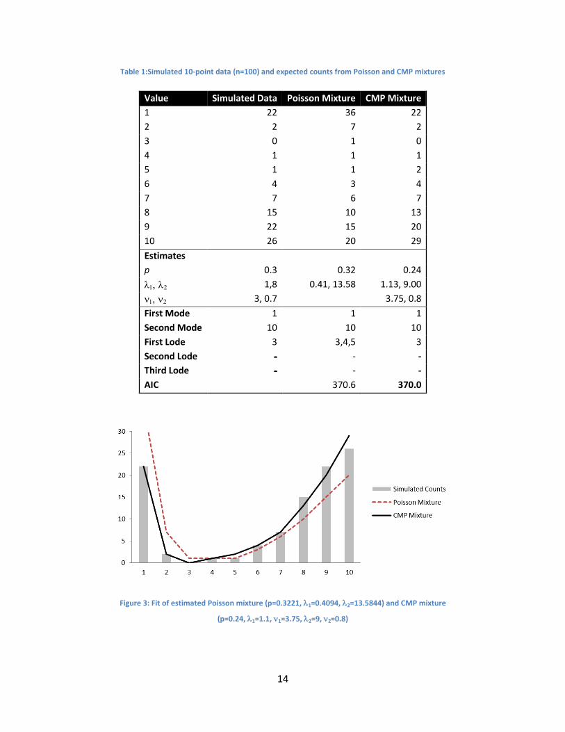
parameter p=0.3. Figure 3 shows the empirical distribution for 100 observations simulated from

this distribution. We see a mode at 1 and another at 10. We first fit a Poisson mixture, resulting

in the fit shown in Table 1 and Figure 3. As can be seen, the Poisson mixture properly captures

the two modes, but their peak magnitudes are incorrectly flipped (thereby identifying the

highest peak at 1); it also does not capture the single lode at 3, but rather estimates a longer

dip throughout 3,4,5. Finally, the estimated overall U-shape is also distorted. Note that the

three estimated parameters (and p) are quite close to the generating ones, yet the

resulting fit is poor.

We then fit a CMP mixture using the algorithm described in Section 4. The results are shown in

Table 1 and Figure 3. The fit appears satisfactory in terms of correctly capturing the two modes

and single load as well as the magnitudes of the peaks and dip. Note that the AIC statistic is very

close to that from the Poisson mixture, yet the two models are visibly very different in terms of

capturing modes, lodes, magnitudes and the overall shape.

Although the good fit of the CMP mixture might not be surprising (because the data were

generated from a CMP mixture), it is reassuring that the algorithm converges to a solution with

good fit. We also note that the estimated parameters are close to the generating parameters.

Finally, we note that the runtime was about a minute.

14

Table 1:Simulated 10-point data (n=100) and expected counts from Poisson and CMP mixtures

Value Simulated Data Poisson Mixture CMP Mixture

1 22 36 22

2 2 7 2

3 0 1 0

4 1 1 1

5 1 1 2

6 4 3 4

7 7 6 7

8 15 10 13

9 22 15 20

10 26 20 29

Estimates

p 0.3 0.32 0.24

1,8 0.41, 13.58 1.13, 9.00

3, 0.7 3.75, 0.8

First Mode 1 1 1

Second Mode 10 10 10

First Lode 3 3,4,5 3

Second Lode - - -

Third Lode - - -

AIC 370.6 370.0

Figure 3: Fit of estimated Poisson mixture (p=0.3221, 1=0.4094, 2=13.5844) and CMP mixture

(p=0.24, 1=1.1, 1=3.75, 2=9, 2=0.8)

15

Identifiability

Identifiability can be a challenge in some cases and a blessing in other cases. When the goal is

to capture the underlying dispersion level, then identifiability is obviously a challenge. However,

for descriptive or predictive goals, the ability to capture the empirical distribution with more

than one model allows for flexibility in choosing models based on other important

considerations such as computational speed or predictive accuracy.

Exploring the likelihood function, which is quite flat in the area of the maximum, we observe an

identifiability issue. In particular, we find multiple parameter combinations that yield very

similar results in terms of the estimated distribution. For instance, in our above example, the

estimated CMP mixture is of one under-dispersed CMP ( and one over-

dispersed CMP ( with mixing parameter p=0.24. By replacing only the over-

dispersed CMP with the under-dispersed CMP( we obtain a nearly identical fit,

as shown in Figure 4 and Table 2 (“CMP Mixture 2”). Mixture 2 is inferior to Mixture 1 only in

terms of detecting lode 1 (indicating a lode at 1-2), but otherwise very similar. Another similar

fit can be achieved by slightly modifying the two parameters to (“CMP Mixture

3”). In other words, we can achieve similar results by combining different dispersion levels. In

this example, we are able to achieve similar results by combining an over- and an under-

dispersed CMP and by combining two under-dispersed CMPs.

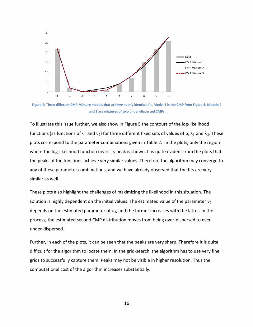
Table 2: Three CMP mixtures fitted to the same data, with very similar fit

Value Counts CMP Mixture 1

(

CMP Mixture 2

(

CMP Mixture 3

(

1 22 22 21 22

2 2 2 3 2

3 0 0 0 0

4 1 1 0 0

5 1 2 1 1

6 4 4 4 4

7 7 8 8 8

8 15 13 14 14

9 22 20 21 21

10 26 28 28 28

16

Figure 4: Three different CMP Mixture models that achieve nearly identical fit. Model 1 is the CMP from Figure 6. Models 2

and 3 are mixtures of two under-dispersed CMPs

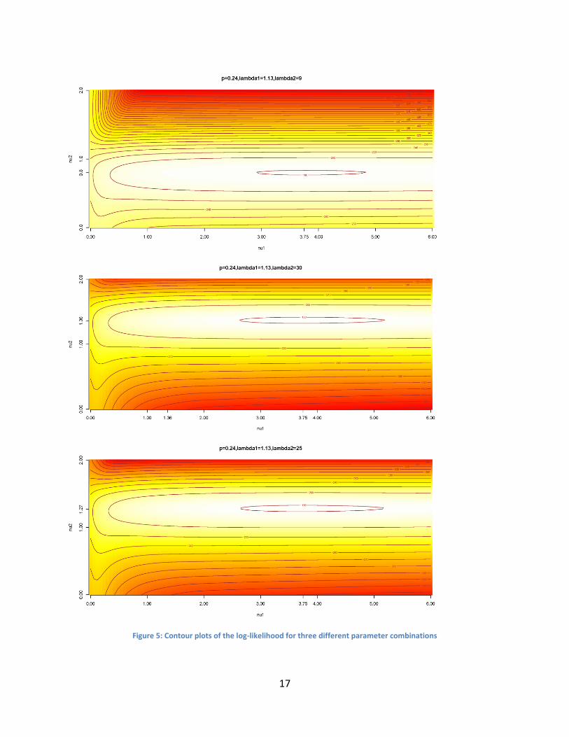
To illustrate this issue further, we also show in Figure 5 the contours of the log-likelihood

functions (as functions of and ) for three different fixed sets of values of p, and . These

plots correspond to the parameter combinations given in Table 2. In the plots, only the region

where the log-likelihood function nears its peak is shown. It is quite evident from the plots that

the peaks of the functions achieve very similar values. Therefore the algorithm may converge to

any of these parameter combinations, and we have already observed that the fits are very

similar as well.

These plots also highlight the challenges of maximizing the likelihood in this situation. The

solution is highly dependent on the initial values. The estimated value of the parameter

depends on the estimated parameter of , and the former increases with the latter. In the

process, the estimated second CMP distribution moves from being over-dispersed to even

under-dispersed.

Further, in each of the plots, it can be seen that the peaks are very sharp. Therefore it is quite

difficult for the algorithm to locate them. In the grid-search, the algorithm has to use very fine

grids to successfully capture them. Peaks may not be visible in higher resolution. Thus the

computational cost of the algorithm increases substantially.

17

Figure 5: Contour plots of the log-likelihood for three different parameter combinations

18

3.2 Example 2: Bimodal distribution on 15-point scale

To further illustrate the ability of the CMP mixture to identify the two modes and adequately

capture their frequency, as well as dips and overall shape, we further simulated two sets of 15-

point scale data, with n=1,000 for each set.

Table 3, Table 4, Figure 6 and Figure 7 present the simulated data, the fitted Poisson mixture

and the fitted CMP mixture.

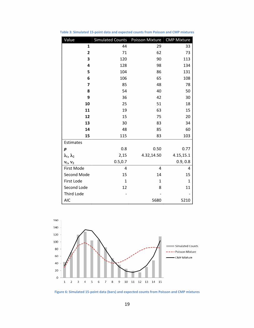
In the first example (Table 3 and Figure 6), both Poisson and CMP mixtures correctly identify

the first mode (at 4), but the CMP estimates the corresponding peak much more accurately

than the Poisson mixture. The second mode (at 15) is only identified correctly by the CMP

mixture, whereas the Poisson mixture indicates a neighboring value (14) as the second mode. In

terms of dips, the first lode (1) is identified by both models. However, for lode2=12 the Poisson

estimate is far away at 8, while the CMP estimate is at the neighboring 11. Overall, the shape

estimated by the CMP is dramatically closer to the data than the shape estimated by the

Poisson mixture.

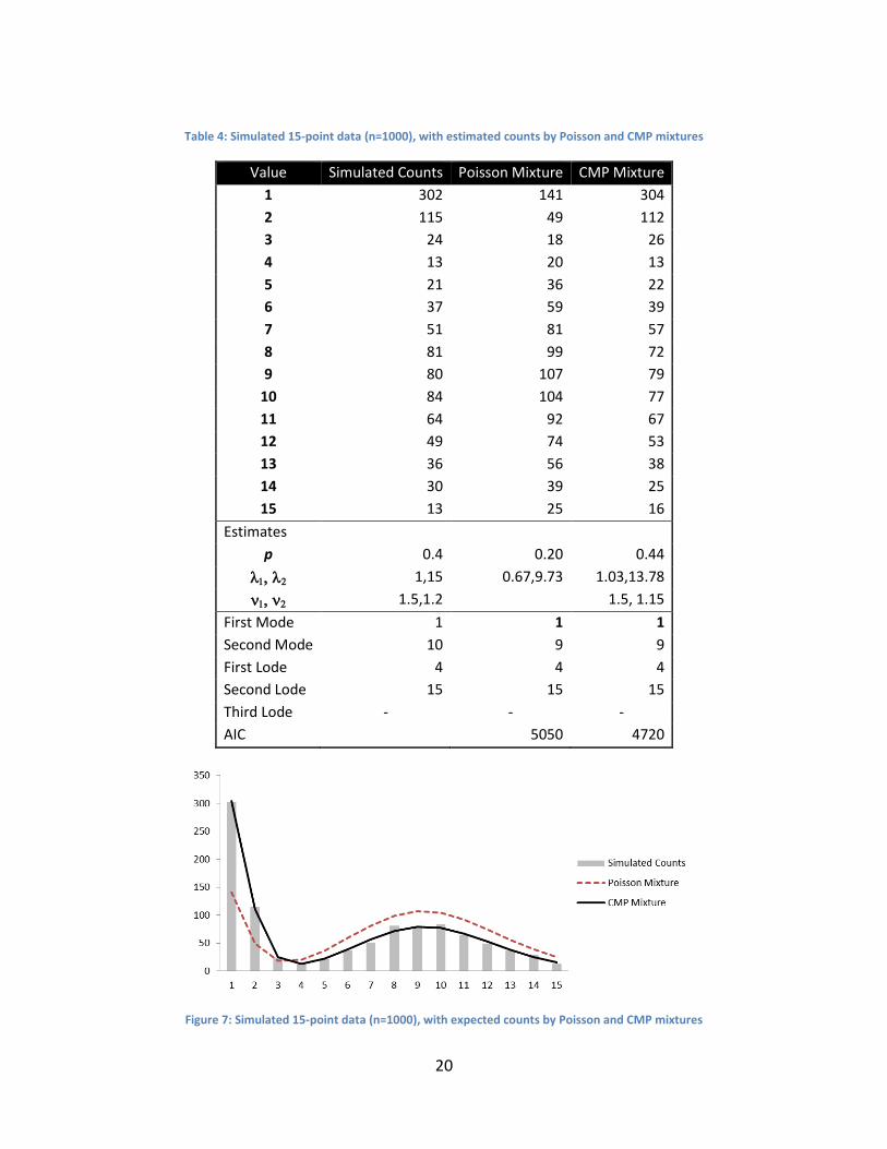
The second example (Table 4 and Figure 7) illustrates the dramatic under-estimation of a

mode’s peak magnitude using the Poisson mixture. In this example, while both Poisson and

CMP mixtures reasonably capture the modes and lodes (with the CMP capturing them more

accurately), they differ significantly in their estimate for the magnitude of the first peak. Such

data shapes would not be uncommon in rating data.

19

Table 3: Simulated 15-point data and expected counts from Poisson and CMP mixtures

Value Simulated Counts Poisson Mixture CMP Mixture

1 44 29 33

2 71 62 73

3 120 90 113

4 128 98 134

5 104 86 131

6 106 65 108

7 85 48 78

8 54 40 50

9 36 42 30

10 25 51 18

11 19 63 15

12 15 75 20

13 30 83 34

14 48 85 60

15 115 83 103

Estimates

p 0.8 0.50 0.77

2,15 4.32,14.50 4.15,15.1

0.5,0.7 0.9, 0.8

First Mode 4 4 4

Second Mode 15 14 15

First Lode 1 1 1

Second Lode 12 8 11

Third Lode - - -

AIC 5680 5210

Figure 6: Simulated 15-point data (bars) and expected counts from Poisson and CMP mixtures

20

Table 4: Simulated 15-point data (n=1000), with estimated counts by Poisson and CMP mixtures

Value Simulated Counts Poisson Mixture CMP Mixture

1 302 141 304

2 115 49 112

3 24 18 26

4 13 20 13

5 21 36 22

6 37 59 39

7 51 81 57

8 81 99 72

9 80 107 79

10 84 104 77

11 64 92 67

12 49 74 53

13 36 56 38

14 30 39 25

15 13 25 16

Estimates

p 0.4 0.20 0.44

1,15 0.67,9.73 1.03,13.78

1.5,1.2 1.5, 1.15

First Mode 1 1 1

Second Mode 10 9 9

First Lode 4 4 4

Second Lode 15 15 15

Third Lode - - -

AIC 5050 4720

Figure 7: Simulated 15-point data (n=1000), with expected counts by Poisson and CMP mixtures

21

4 Application to Real Data

We now return to the three real-life examples presented in Section ‎1. In each case, we fit a

CMP mixture, evaluate its fit, and compare it to a Poisson mixture.

4.1 Example 1: Online ratings

Recall the Tripadvisor.com 5-point rating of Druk Hotel from Section ‎1.1. The results of fitting a

Poisson mixture and CMP mixture are shown in Table 5 and Figure 8. A visual inspection shows

that the CMP mixture outperforms the Poisson mixture in terms of capturing the overall shape

of the distribution.

Table 5: Observed and fitted counts for Druk Hotel online ratings

Rating Data Poisson Mixture CMP Mixture

terrible 4 9 3

poor 2 9 5

average 10 9 8

very good 17 10 14

excellent 17 13 19

Estimates

p 0.22 0.09

1.58, 6.91 0.91, 5.23

0.5, 0.8

First Mode very good, excellent excellent excellent

Second Mode terrible - -

Dip Location poor terrible, poor, average terrible

AIC 178.3156 171.1

Figure 8: Observed and fitted Poisson and CMP mixture counts for Druk Hotel online rating example

22

In this example and in ratings applications in general, it is possible to flip the order of the values

from low to high or from high to low. Here, we can re-order the ratings from “excellent” to

“terrible”. Next, we show the results of fitting Poisson and CMP mixtures to the flipped ratings

(see Table 6 and Figure 9). It is interesting to note that for the CMP mixture the estimates

slightly change, but the fitted counts remain unchanged. In contrast, for the Poisson mixture,

flipping the order yields a slightly better fit in terms of shape.

Table 6: Poisson and CMP mixtures fitted to the flipped ratings (excellent to terrible)

Rating Data Poisson Mixture CMP Mixture

excellent 17 15 19

very good 17 14 14

average 10 10 8

poor 2 7 5

terrible 4 4 3

Estimates

p 0.55 0.88

1.38,3.38 1.03, 4.68

0.6, 0.8

First Mode very good, excellent excellent excellent

Second Mode terrible - -

Dip Location poor terrible, poor, average terrible

AIC 206.8623 204.1

Figure 9: Poisson and CMP mixtures, fitted to the flipped ratings (excellent to terrible)

23

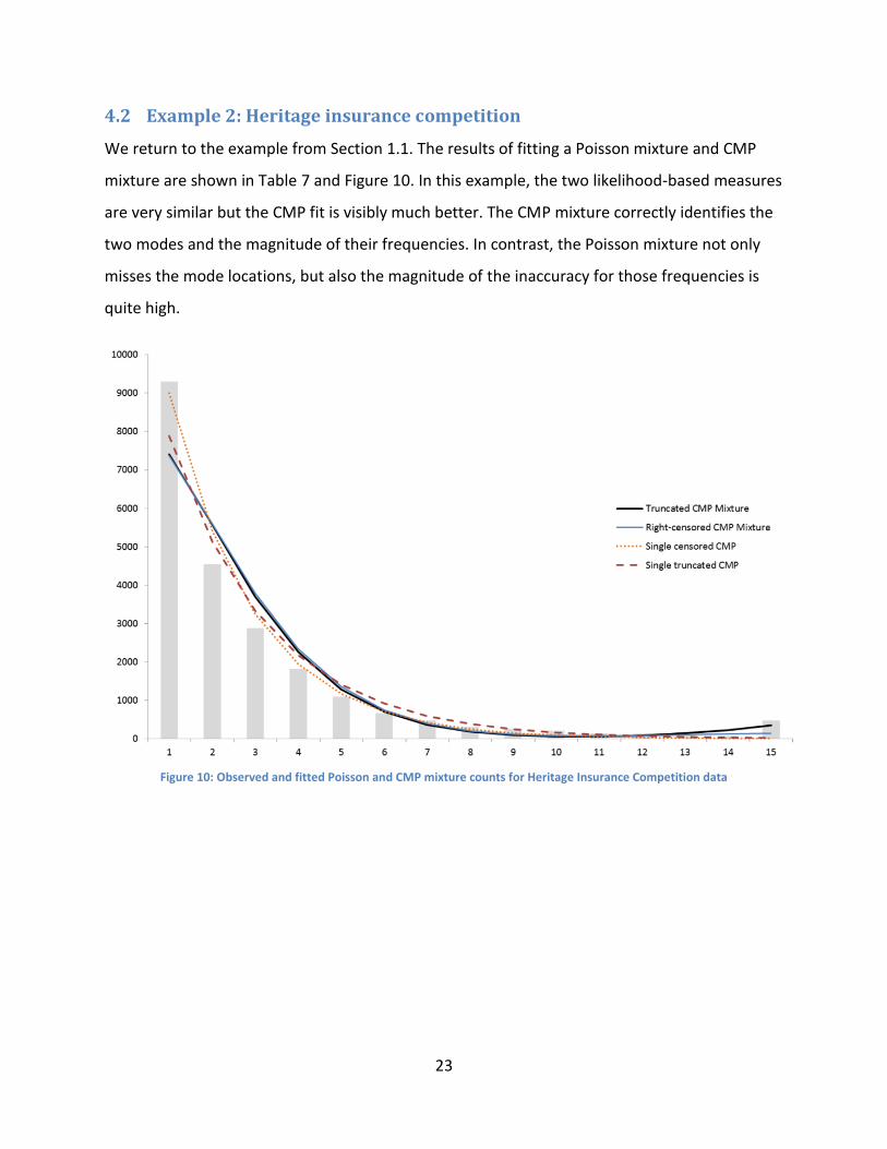
4.2 Example 2: Heritage insurance competition

We return to the example from Section ‎1.1. The results of fitting a Poisson mixture and CMP

mixture are shown in Table 7 and Figure 10. In this example, the two likelihood-based measures

are very similar but the CMP fit is visibly much better. The CMP mixture correctly identifies the

two modes and the magnitude of their frequencies. In contrast, the Poisson mixture not only

misses the mode locations, but also the magnitude of the inaccuracy for those frequencies is

quite high.

Figure 10: Observed and fitted Poisson and CMP mixture counts for Heritage Insurance Competition data

24

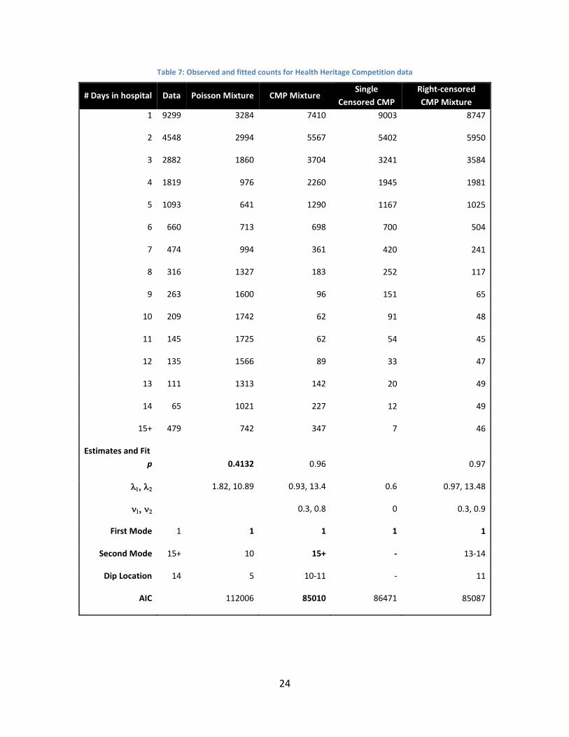
Table 7: Observed and fitted counts for Health Heritage Competition data

# Days in hospital Data Poisson Mixture CMP Mixture Single

Censored CMP

Right-censored

CMP Mixture 1 9299 3284 7410 9003 8747

2 4548 2994 5567 5402 5950

3 2882 1860 3704 3241 3584

4 1819 976 2260 1945 1981

5 1093 641 1290 1167 1025

6 660 713 698 700 504

7 474 994 361 420 241

8 316 1327 183 252 117

9 263 1600 96 151 65

10 209 1742 62 91 48

11 145 1725 62 54 45

12 135 1566 89 33 47

13 111 1313 142 20 49

14 65 1021 227 12 49

15+ 479 742 347 7 46

Estimates and Fit

p 0.4132 0.96 0.97

1.82, 10.89 0.93, 13.4 0.6 0.97, 13.48

0.3, 0.8 0 0.3, 0.9

First Mode 1 1 1 1 1

Second Mode 15+ 10 15+ - 13-14

Dip Location 14 5 10-11 - 11

AIC 112006 85010 86471 85087

25

Truncated Mixture vs. Censored Models

In this particular example, the data are right-censored at 15, with all 15+ counts given in

censored form. We therefore compare the truncated CMP mixture to two alternative censored

models: (1) a single right-censored CMP (with support starting at 1), and (2) a mixture of two

right-censored CMP distributions. The log-likelihood function for a right-censored CMP can be

written as follows:

∑ ( ) ( ) ( ) (8)

∑( )

[ ( )] ( )

where =1 indicates that observation i is right-censored, and otherwise =0; In addition,

( ) ∑

( )

Results for fitting the two censored models are given in the right columns of Table 7. Results

for a single interval-censored CMP model were identical to the single shifted and right-censored

CMP model.

In terms of fit, while the single censored CMP best captures the first mode at 1, it fails to

capture the bimodal shape with a dip at 14 and a second mode at 15. A mixture of censored

CMP variables performs very similar to the truncated mixture except for missing the magnitude

of the second mode at 15+.

We note that computationally, it is much easier to compute a mixture of truncated CMP

distributions over censored CMP distributions, because in the latter case the Z function is

computed over a finite range whereas the censored case requires computing the normalizing

constant Z over an infinite range (see Minka et al., 2003). From this aspect, if the truncated

mixture performs sufficiently well, it might be advantageous computationally in cases where

the data are not necessarily truncated by nature.

26

5 Discussion and Future Directions

Discrete data often exhibit bimodality that is difficult to model with standard distributions. A

natural choice would be a mixture of two (or more) Poisson distributions. However due to the

presence of under- or over-dispersion, often the Poisson mixture appears to be inadequate. The

more general CMP distribution can capture under- or over-dispersion in the data. Therefore a

mixture of CMP distributions (if necessary, properly truncated) may be appropriate to model

such data.

The usual EM algorithm for fitting mixtures of distribution can be employed in this scenario.

However, as the CMP distribution has an additional parameter (compared to the Poisson

distribution), the maximization of the likelihood is nontrivial. In the absence of closed form

solutions, iterative numerical algorithms are used for this purpose. An innovative two-step

optimization with more than one possible initialization of the parameters has been suggested

to ensure and speed up the convergence of the resulting algorithm. In our experiments, the

proposed algorithm for fitting CMP mixture models takes less than two minutes even for very

large datasets (such as the Heritage Competition data). Further reduction in runtime may be

possible by invoking more efficient optimization techniques.

An interesting property was observed while fitting the mixture of CMP distributions. If the

ordering of the labels are reversed in case of (for example) consumer evaluation data, the fit

appears to be very similar to the original one. This was not the case for the mixture of Poisson

distributions. However this has to be more thoroughly investigated.

Though there is an inherent identifiability issue in the case of CMP mixture models, as there

may be more than one combination of parameters of the underlying distributions yielding

very similar shapes for the resulting mixtures, it does not cause any problem in terms of

prediction. Rather it provides flexibility in choosing a model among several competing ones for

improving predictive accuracy. This property is also advantageous in terms of bounding the

parameter space in the grid search, whereby we can set relatively low upper bounds on and

values. Even for purposes of descriptive modeling, where we are interested in an

27

approximation of the empirical distribution shape (location of peaks, etc.), the non-

identifiability issue is not a challenge. It does, however, pose a challenge if the goal is

identifying the underlying dispersion levels of the CMP distributions.

We note that the identifiability issue pertains only to combinations of andand does not

extend to the mixing parameter p in the sense that we did not encounter any situation where a

different combination of the 5 parameters yielded similar fits. This is perhaps due to the fact

that we do get a closed form solution for p. Never did we get a poor estimate of this mixing

parameter in any of the simulations. In other words, p identified the bimodality (when it is

clearly present) without failure. The lack of fit due to a wrong choice of p cannot be

compensated by changing the values of the other parameters.

To illustrate the predictive performance of a CMP mixture with a real example, we split the

Heritage Healthcare data into training and holdout data sets. The training data consist of data

from year 2 and the holdout period is year 3. We fit a CMP mixture to the training period and

generate predictions for the holdout period (see Figure 11). To show how the non-

identifiability can be advantageous in terms of generating robust predictions, we fit another

CMP mixture with slightly different parameters (achieved by using different initial values). The

second model yields a nearly-identical predictive distribution. The two CMP mixture models

also yield similar AIC values: 44965 and 44980, compared to a Poisson mixture which yields

AIC=62204. Yet, AIC and other predictive metrics that are common for continuous data are not

always useful for discrete data (e.g., Czado et al. 2009). An important future direction is

therefore to develop and assess predictive metrics and criteria for bimodal discrete data, and in

particular within the context of truncated mixture models that can capture bimodality.

While Poisson and CMP distributions are designed for modeling count data, we note their

usefulness in the context of bimodal discrete data that can include not only count data but also

ordinal data such as ratings and rankings. Our illustrations show that using the CMP mixture can

adequately capture the distribution of a sample from Likert-type scales and star ratings. We

also note that a truncated CMP mixture can provide a useful alternative to censored CMP

28

models, when modeling censored over/under-dispersed count data. It can be advantageous in

terms of capturing the bimodal shape and especially from a computational standpoint.

Figure 11: Predictive accuracy evaluation. Predictions from two CMP mixture models fitted to the Health Heritage training

period (Year 2) compared to actual counts in holdout period (Year 3).

In our mixture scenario, observations are assumed to arise from a mixture distribution where it

is not possible to identify which observation came from which original distribution (CMP1 or

CMP2). Related work by Sellers and Shmueli (2012) uses a CMP regression formulation where

predictor information is used to try and separate observations into dispersion groups and

estimate the separate group-level dispersion. They show that mixing different dispersion levels

can result in data with unexpected dispersion magnitude (e.g., mixing two under-dispersed

CMPs can result in an apparent over-dispersed distribution). Our work differs from that work

not only in looking at truncated CMPs, but also in the focus on predictive and descriptive

29

modeling, where the goal is to find a parsimonious approximation for the observed empirical

distribution.

One direction for expanding our work, is generalizing to k (>2) mixtures. In that case, we can

write the likelihood and the E & M steps without any problem. Again the equations for the

mixing parameters p1, p2, ..., pk-1 will yield closed form solutions. The difficulty will be the grid-

search over 2k parameters. It is expected that the same strategy of fixing p1, p2, ..., pk-1 and the

’s first and optimizing over the ’s will work better. However the effectiveness of the grid-

search has to be tested in those situations.

This novel idea of CMP mixture modeling may also be extended to regression problems

involving discrete bimodal data. For example, the Health Heritage example that we used comes

from a larger contest for predicting length of stay at the hospital, where the data included

many potential predictor variables. If the dependent variable shows bimodality, as in the case

of the truncated “days in hospital” variable, the ordinary CMP regression might not be able to

capture this feature. CMP mixture models may be very useful in this scenario. Another potential

extension is to consider mixtures of more than two CMP distributions. Sellers and Shmueli

(2010) considered CMP regression models for censored data. It would be interesting to explore

the possibility of using a CMP mixture model in this context as well.

Acknowledgements

The authors thank three anonymous referees and the Associate Editor for providing thought-

provoking suggestions which led to valuable additions to the paper.

30

6 References

Czado C, Gneiting T, and Held L (2009), “Predictive Model Assessment for Count Data”,

Biometrics, vol. 65(4), pp. 1254-1261.

Dempster AP, Laird NM, and Rubin DB (1977), "Maximum Likelihood from Incomplete Data via

the EM Algorithm", Journal of the Royal Statistical Society, Series B, vol. 39(1), pp. 1–38

Hilbe JM (2011), Negative Binomial Regression, 2nd edition, Cambridge University Press

McLachlan, GJ (1997) “On the EM algorithm for overdispersed count data”, Statistical Methods

in Medical Research, vol. 6, pp. 76-98.

Minka, TP, Shmueli G, Kadane JB, Borle S, and Boatwright P (2003), “Computing with the COM-

Poisson distribution”, Technical Report 776. Dept of Statistics, Carnegie Mellon University

Sellers KF, Borle S and Shmueli G (2012) “The CMP Model for Count Data: A Survey of Methods

and Applications”, Applied Stochastic Models in Business and Industry, vol. 28(2), pp. 104-

116.

Sellers KF and Shmueli G (2010), “Predicting Censored Count Data with CMP Regression”,

Working Paper RHS 06-129, Smith School of Business, University of Maryland.

Sellers KF and Shmueli G (2010), “A Flexible Regression Model for Count Data”, Annals of

Applied Statistics, vol. 4(2), pp. 943-961.

Sellers KF and Shmueli G (2013), “Data Dispersion: Now You See it... Now You Don't”,

Communications in Statistics: Theory and Methods, vol. 42(17), pp. 3134-3147.

Shmueli G, Minka TP, Kadane JB, Borle, S, and Boatwright, P (2005) “A useful distribution for

fitting discrete data: revival of the Conway–Maxwell–Poisson distribution”, Journal of The

Royal Statistical Society, Series C (Applied Statistics), vol. 54(1), pp. 127-142.

Wu, CFJ (1983), “On the convergence properties of the EM algorithm”, The Annals of Statistics,

vol. 11(1), pp. 95-103.

31

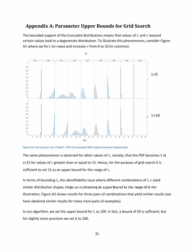
Appendix A: Parameter Upper Bounds for Grid Search

The bounded support of the truncated distributions means that values of and beyond

certain values lead to a degenerate distribution. To illustrate this phenomenon, consider Figure

A1 where we fix (in rows) and increase from 0 to 10 (in columns):

Figure A1: Increasing for a fixed . PDF of truncated CMP mixture becomes degenerate

The same phenomenon is observed for other values of , namely, that the PDF becomes 1 at

x=15 for values of greater than or equal to 15. Hence, for the purpose of grid search it is

sufficient to set 15 as an upper bound for the range of .

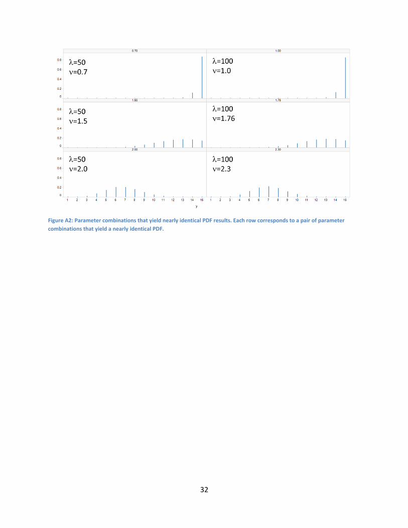
In terms of bounding , the identifiability issue where different combinations of yield

similar distribution shapes, he

illustration, Figure A2 shows results for three pairs of combinations that yield similar results (we

have obtained similar results for many more pairs of examples).

In our algorithm, we set the upper bound for as 100. In fact, a bound of 50 is sufficient, but

for slightly more precision we set it to 100.

32

Figure A2: Parameter combinations that yield nearly identical PDF results. Each row corresponds to a pair of parameter

combinations that yield a nearly identical PDF.