Modeling and Simulating Social Systems with …851-0585-04L – Modeling and Simulating Social Systems with MATLAB Lecture 4 – Cellular Automata Chair of Sociology, in particular

2012-10-15 © ETH Zürich |

851-0585-04L – Modeling and Simulating Social Systems with MATLAB

Lecture 4 – Cellular Automata

© ETH Zürich |

Chair of Sociology, in particular of

Modeling and Simulation

Karsten Donnay and Stefano Balietti

2012-10-15 K. Donnay & S. Balietti / [email protected] [email protected] 2

Schedule of the course 24.09. 01.10. 08.10. 15.10. 22.10. 29.10. 05.11. 12.11. 19.11. 26.11. 03.12. 10.12. 17.12.

Introduction to MATLAB

Introduction to social-science modeling and simulations

Working on projects (seminar thesis)

Handing in seminar thesis and giving a presentation

Create and Submit a Research Plan DEADLINE: 22.10.


Projects – Suggested Topics 1 Traffic Dynamics 9 Evacuation Bottleneck 17 Self-organized Criticality 25 Facebook

2 Civil Violence 10 Friendship Network Formation

18 Social Networks Evolution

26 Sequential Investment Game

3 Collective Behavior 11 Innovation Diffusion 19 Task Allocation & Division of Labor

27 Modeling the Peer Review System

4 Disaster Spreading 12 Interstate Conflict 20 Artificial Financial Markets

28 Modeling Science

5 Emergence of Conventions

13 Language Formation 21 Desert Ant Behavior 29 Simulation of Networks in Science

6 Emergence of Cooperation

14 Learning 22 Trail Formation 30 Opinion Formation in Science

7 Emergence of Culture 15 Opinion Formation 23 Wikipedia 31 Organizational Learning

8 Emergence of Values 16 Pedestrian Dynamics 24 Social Contagion

2012-10-15 K. Donnay & S. Balietti / [email protected] [email protected]

Goals of Lecture 4: students will 1.  Consolidate their knowledge of dynamical systems,

through brief repetition of the main concepts and revision of the exercises.

2.  Get familiar with how and why simulation models may contribute to our understanding of complex socio-dynamic processes.

3.  Understand the important concept of Cellular Automata as discrete representations of interactions on an abstract grid (or configuration space).

4.  Implement simple Cellular Automata in MATLAB (Game of Life, Highway Simulation, Epidemics: Kermack-McKendrick model revisited)

4


Repetition   dynamical systems described by a set of differential

equations (example: Lotka-Volterra)   numerical solutions iteratively for instances using 1st

Euler’s Method (example: Kermack-McKendrick)   the values and ranges of parameters critically matter;

they determine which dynamics the model represents (Ex. 2, the ratio of recuperation to infection parameter determines the epidemiological threshold)

  time resolution in Euler Method must be sufficiently high to capture (‘fast’) system dynamics (Ex. 3)

  not all MATLAB-own ODE solvers work equally well for every dynamical system under consideration (Ex. 3)

5


Simulation Models   What do we mean when we speak of

(simulation) models?   Formalized (computational) representation of social,

economic etc. dynamics   Implies reduction of complexity, i.e. usually making

(strong) simplifying assumptions

  Not trying to reproduce reality but rather systematize specific interdependencies of “real” systems

  Formal framework to test and evaluate causal hypotheses against empirical data (or stylized facts)


Simulation Models   Strength of (simulation) models?

  Computational laboratory: test how micro dynamics lead to macro patters

  There are usually no experiments in social sciences but computer models can be a “testing ground”

  Particularly suitable where formal models fail (or where dynamics are too complex for formal modeling)

  Possible to combine empirical input with quantitative validation of both the results and mechanisms


Simulation Models   Weakness of (simulation) models?

  The choice of model parameters, implementation etc. may strongly influence the simulation outcome

  We can only model aspects of a system, i.e. the models are necessarily incomplete & reductionist

  More complex models are NOT necessarily better: dynamics between model components often poorly understood (a known problem in climate modeling)

  Can construct a computational model of virtually anything but hard to verify if you are actually studying a realistic empirical question!


Simulation Models   How to we deal with known limitations?

  Use empirical input and formal optimization to rule out arbitrariness of the model

  Test for implementation- and specification- dependence of simulations

  Validate the model mechanism both with observations and causal theory

  Use empirical data to evaluate the predictive power of the simulation model


Cellular Automaton (plural: Automata)


Cellular Automaton (plural: Automata)   A cellular automaton is a rule, defining how the

state of a cell in a grid is updated, depending on the states of its neighbor cells.

  May be represented as grids with arbitrary dimension.

  Cellular-automata simulations are discrete both in time and space.


Cellular Automaton (plural: Automata)   Simplest example for a (reduced) representation

of an interaction model

  Automata dimensions represent an abstract “distance” that could be spatial, social relations etc.

  Natural micro-to-macro link from interactions between cells to patterns visible in the automaton


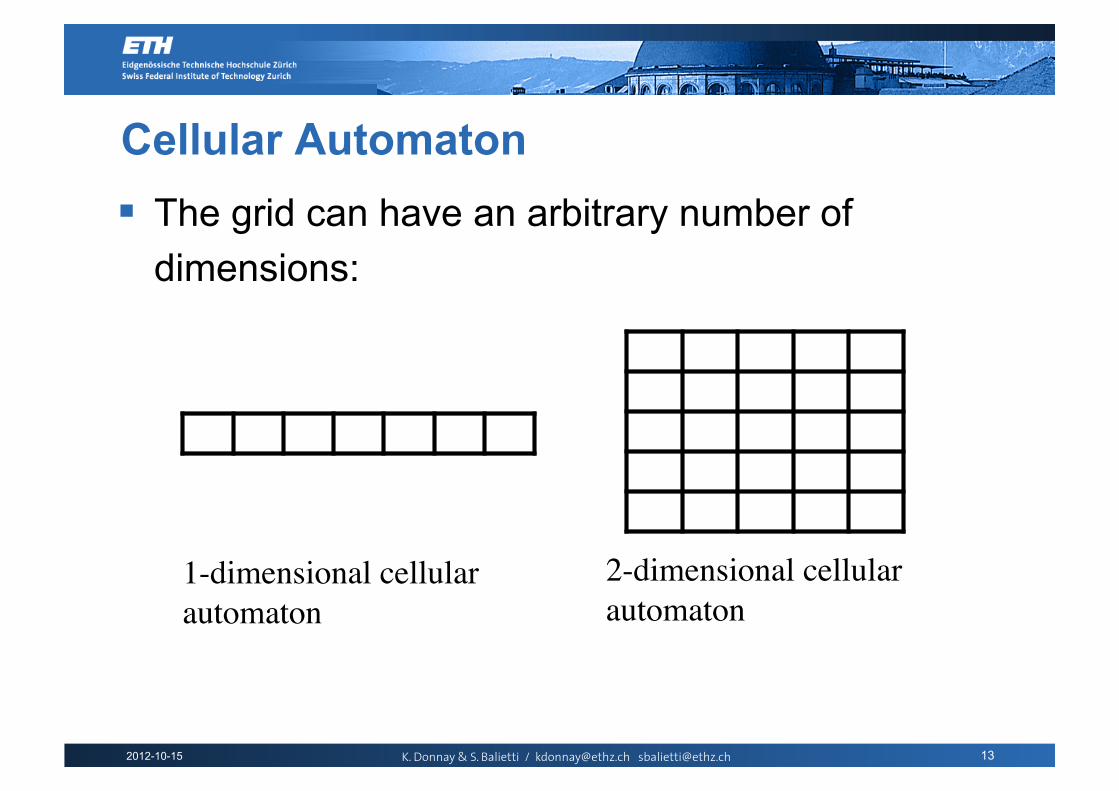
Cellular Automaton   The grid can have an arbitrary number of

dimensions:

1-dimensional cellular automaton

2-dimensional cellular automaton


Moore Neighborhood   The cells are interacting with each neighbor

cells, and the neighborhood can be defined in different ways, e.g. the Moore neighborhood:

1st order Moore neighborhood 2nd order Moore neighborhood


Von-Neumann Neighborhood   The cells are interacting with each neighbor cells,

and the neighborhood can be defined in different ways, e.g. the Von-Neumann neighborhood:

1st order Von-Neumann ��neighborhood

2nd order Von-Neumann ��neighborhood


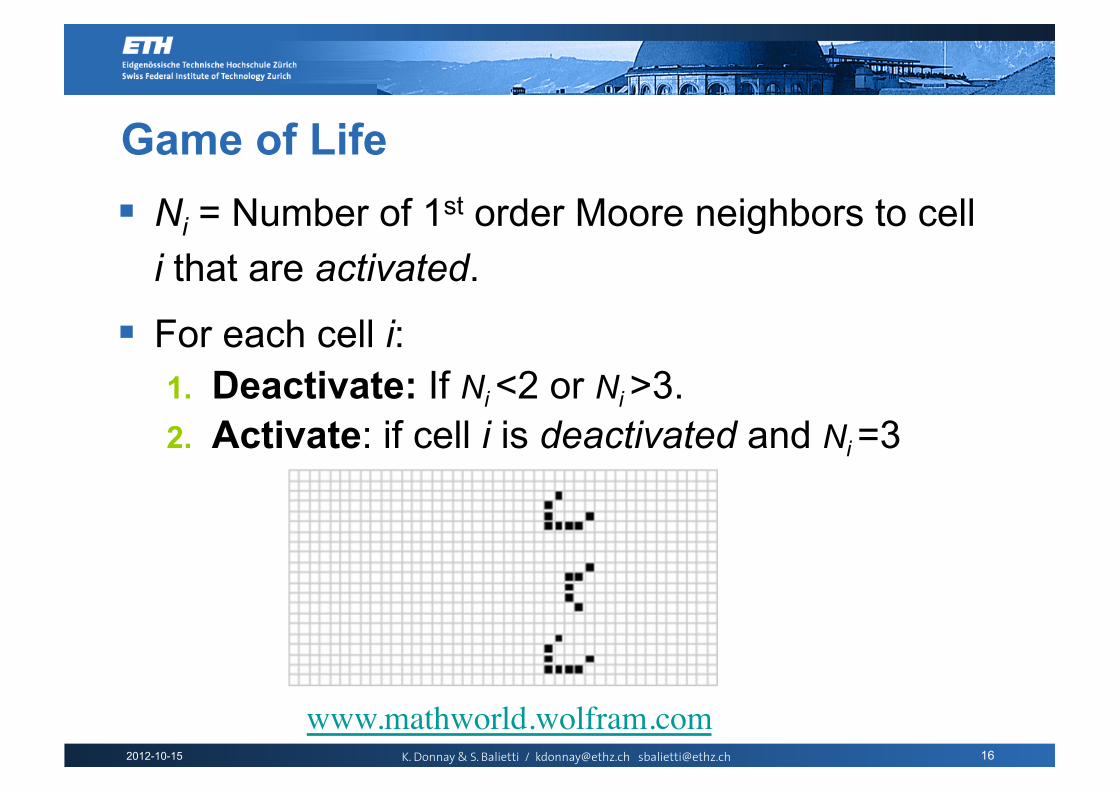
Game of Life   Ni = Number of 1st order Moore neighbors to cell

i that are activated.

  For each cell i: 1.  Deactivate: If Ni <2 or Ni >3. 2.  Activate: if cell i is deactivated and Ni =3

www.mathworld.wolfram.com


Game of Life   Want to see the Game of Life in action? Type:

life!


Game of Life Patterns: can you find them?   Ants

  B-52

  Blinker puffer

  Diehard

  Canada goose

  Gliders by the dozen

  Kok’s galaxy

  Rabbits

  R2D2

  Spacefiller

  Wasp

  Washerwoman

  …

18


Cellular Automata: A New Kind of Science?

  A thorough study of all 256 “behavioral” rules of a 1-D cellular automata.


Cellular Automata: A New Kind of Science?


Cellular Automaton: Principles 1.  Self Organization: Patterns appear without a

designer

2.  Emergence: Gliders, glider guns, wasps, rabbits appear

3.  Complexity: Simple rules produce complex phenomena


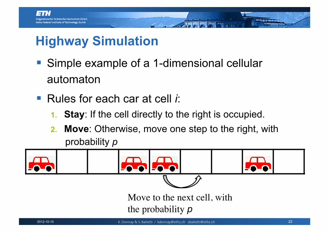
Highway Simulation   Simple example of a 1-dimensional cellular

automaton

  Rules for each car at cell i: 1.  Stay: If the cell directly to the right is occupied. 2.  Move: Otherwise, move one step to the right, with

probability p

Move to the next cell, with the probability p


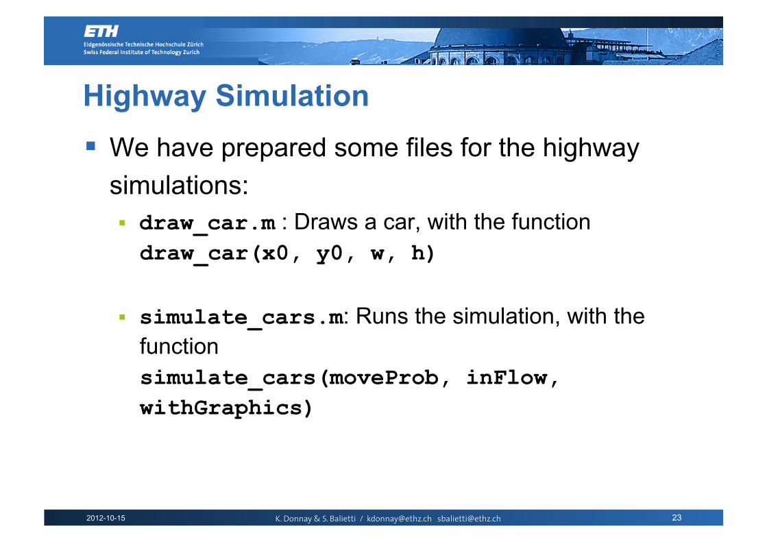
Highway Simulation   We have prepared some files for the highway

simulations:   draw_car.m : Draws a car, with the function draw_car(x0, y0, w, h)

  simulate_cars.m: Runs the simulation, with the function simulate_cars(moveProb, inFlow, withGraphics)


Highway Simulation   Running the simulation is done like this: simulate_cars(0.9, 0.2, true)


Kermack-McKendrick Model   In lecture 3, we introduced the Kermack-

McKendrick model, used for simulating disease spreading.

  We will now implement the model again, but this time instead of using differential equations we define it within the cellular-automata framework.


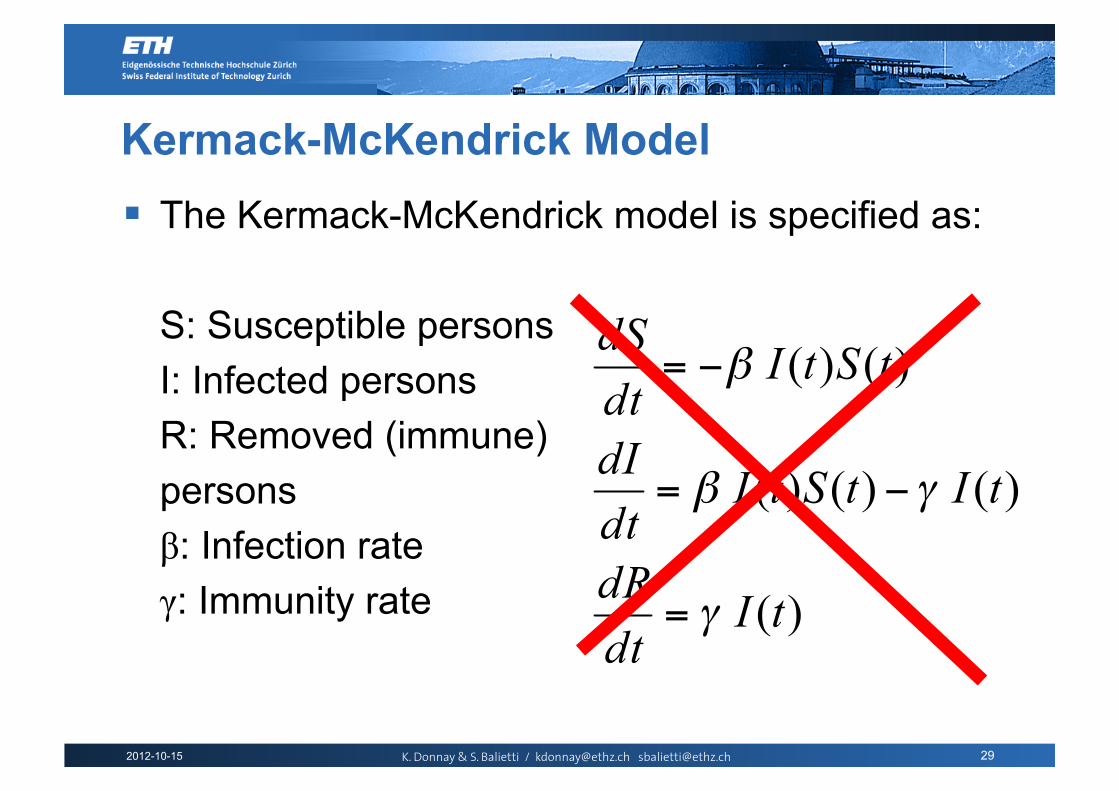
Kermack-McKendrick Model   The Kermack-McKendrick model is specified as:

S: Susceptible persons I: Infected persons R: Removed (immune) persons β: Infection rate γ: Immunity rate

S

I R

β transmission

γ recovery















For the MATLAB implementation, we need to decode the states {S, I, R}={0, 1, 2} in a matrix x.

S S S S S S S I I I S S S S I I I I S S S R I I I S S S R I I I S S S I I I S S S S I S S S S S S

0 0 0 0 0 0 0 1 1 1 0 0 0 0 1 1 1 1 0 0 0 2 1 1 1 0 0 0 2 1 1 1 0 0 0 1 1 1 0 0 0 0 1 0 0 0 0 0 0



We now define a 2-dimensional cellular-automaton, by defining a grid (matrix) x, where each of the cells is in one of the states:   0: Susceptible   1: Infected   2: Recovered


Kermack-McKendrick Model   Define microscopic rules for Kermack-

McKendrick model:

In every time step, the cells can change states according to:

  A Susceptible individual can be infected by an Infected neighbor with probability β, i.e. State 0 -> 1, with probability β.

  An individual can recover from an infection with probability γ, i.e. State 1 -> 2, with probability γ.


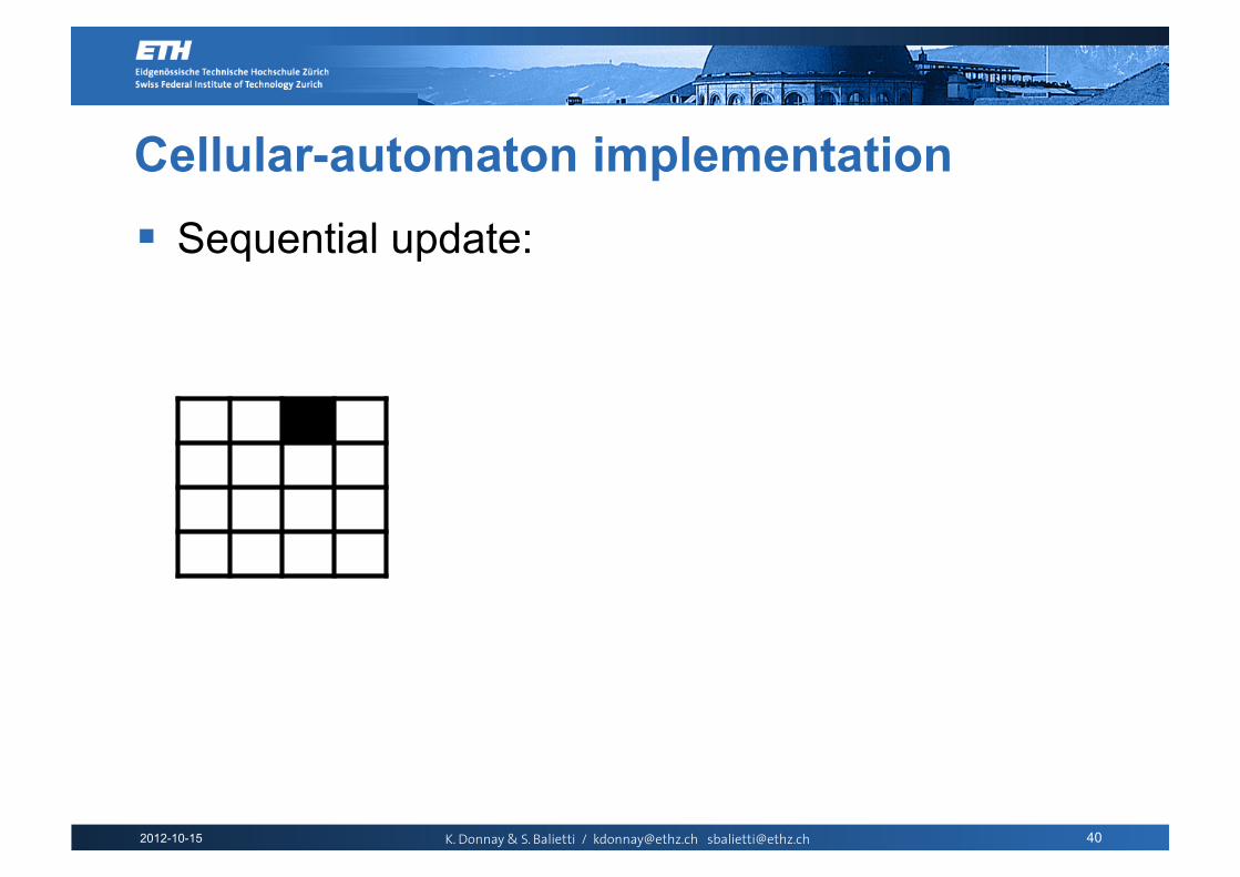
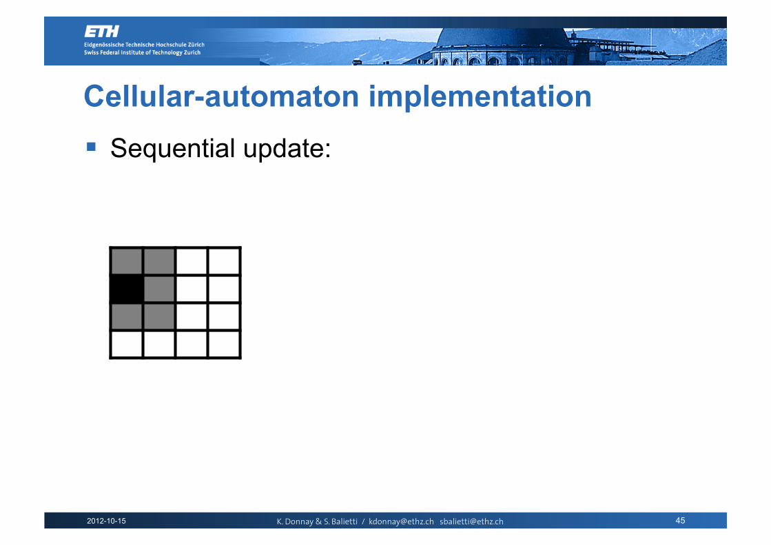
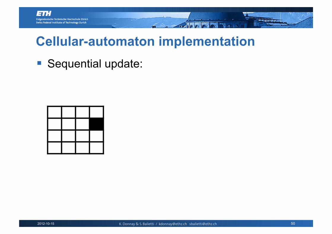
Cellular-Automaton Implementation   Implementation of a 2-dimensional cellular-

automaton model in MATLAB is done like this:

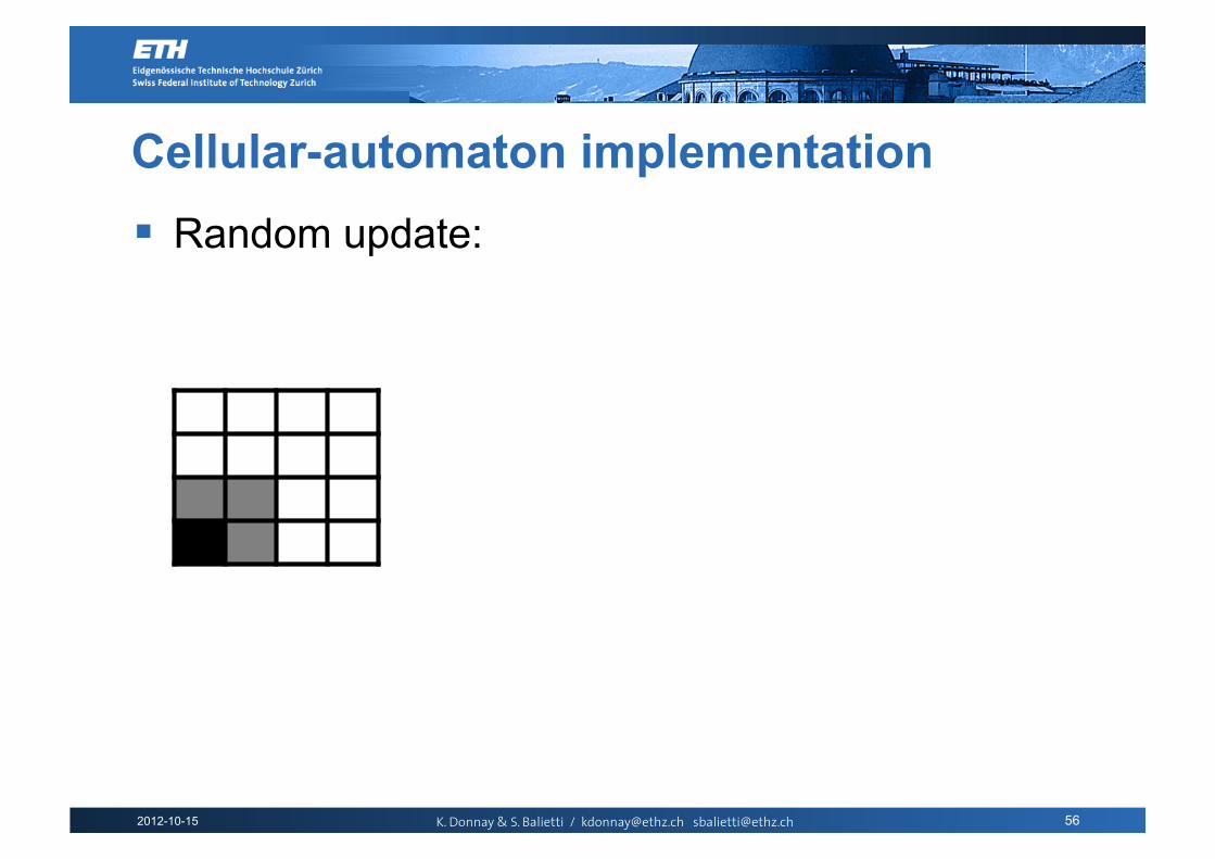
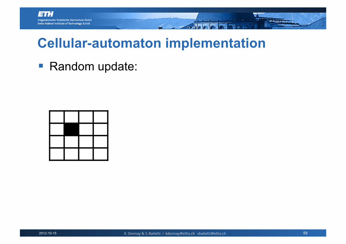
  The iteration over the cells can be done either sequentially, or randomly.

Iterate the time variable, t Iterate over all cells, i=1..N, j=1..N

Iterate over all neighbors, k=1..M

End k-iteration End i-iteration

End t-iteration

…


Cellular-Automaton Implementation   Sequential update:


Cellular-Automaton Implementation   Sequential update:


Cellular-automaton implementation   Sequential update:






























Cellular-automaton implementation   Random update:


















Cellular-automaton implementation   Attention:

  Simulation results may be sensitive to the type of update used!

  Random update is usually preferable but also not always the best solution

  Just be aware of this potential complication and check your results for dependency on the updating scheme!


Boundary Conditions   The boundary conditions can be any of the

following:   Periodic: The grid is wrapped, so that what exits on

one side reappears at the other side of the grid.

  Fixed: Agents are not influenced by what happens at the other side of a border.


Boundary Conditions   The boundary conditions can be any of the

following:

Fixed boundaries Periodic boundaries


MATLAB Implementation of the Kermack-McKendrick Model


MATLAB implementation Set parameter values


MATLAB implementation Define grid, x


MATLAB implementation Define neighborhood


MATLAB implementation Main loop. Iterate the time variable, t


MATLAB implementation Iterate over all cells, i=1..N, j=1..N


MATLAB implementation For each cell i, j: Iterate over the neighbors


MATLAB implementation The model, i.e. updating rule goes here.


Breaking Execution   When running large computations or animations, the

execution can be stopped by pressing Ctrl+C in the main

window:


References   Wolfram, Stephen, A New Kind of Science.

Wolfram Media, Inc., May 14, 2002.

  http://www.bitstorm.org/gameoflife/

  http://ddi.cs.uni-potsdam.de/HyFISCH/Produzieren/lis_projekt/proj_gamelife/ConwayScientificAmerican.htm

  Schelling, Thomas C. (1971). Dynamic Models of Segregation. Journal of Mathematical Sociology 1:143-186.


Exercise 1   Get draw_car.m and simulate_cars.m from

www.soms.ethz.ch/matlab or from https://github.com/msssm/lectures_files

Investigate how the flow (moving vehicles per time step) depends on the density (occupancy 0%..100%) in the simulator. This relation is called the fundamental diagram in transportation engineering.


Exercise 1b   Generate a video of an interesting case in your

traffic simulation.

  We have uploaded an example file, simulate_cars_video.m, and

simulate_cars_video_w7.m


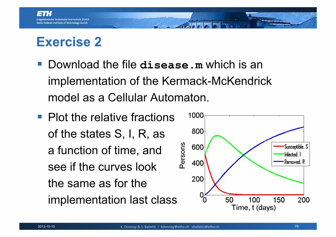
Exercise 2   Download the file disease.m which is an

implementation of the Kermack-McKendrick model as a Cellular Automaton.

  Plot the relative fractions of the states S, I, R, as a function of time, and see if the curves look the same as for the implementation last class


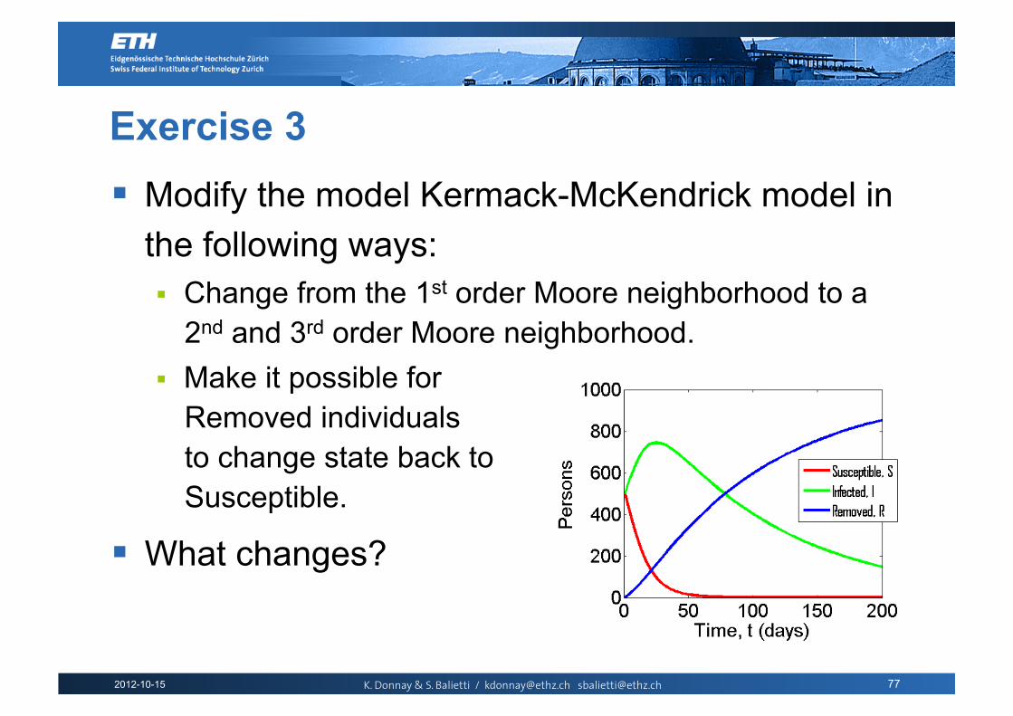
Exercise 3   Modify the model Kermack-McKendrick model in

the following ways:   Change from the 1st order Moore neighborhood to a

2nd and 3rd order Moore neighborhood.   Make it possible for

Removed individuals to change state back to Susceptible.

  What changes?

Documents

Modeling and Simulating Social Systems with …851-0585-04L – Modeling and Simulating Social Systems with MATLAB Lecture 4 – Cellular Automata Chair of Sociology, in particular