COMPUTER ENERGY MODELING TECHNIQUES FOR SIMULATING …

COMPUTER ENERGY MODELING TECHNIQUES FOR SIMULATING LARGE SCALE CORRECTIONAL INSTITUTES IN TEXAS

T. Bou-Saada Research Associate

Energy Systems Laboratory Texas A&M University System

J. Haberl, Ph.D., P.E. Associate Professor

Department of Architecture Texas A&M University System

ABSTRACT Building energy simulation programs have

undergone an increase in use for evaluating energy consumption and energy conservation retrofits in buildings. Utilization of computer simulation programs for large facilities with multiple buildings, however, has been relatively rare. Due to the immense size of certain facilities such as college campuses and correctional institutes, simulating energy consumption for the entire campus and reporting the energy use by individual building is a time consuming task.

Initially, many computer simulation programs were designed to operate on the assumption that the user is simulating one building. Provisions are not usually made to knit together outputs from multiple buildings. Furthermore, programs such as DOE-2 have limits to the number of walls, windows, and zones that can be simulated in one run. This paper presents a methodology to model an entire campus by simulating each building as a single zone consistent with electrical feeders instead of as a separate entity.

Since most simulation programs calculate energy use by means of one-dimensional heat transfer, utilizing this method becomes a practical solution, particularly if the facility does not contain buildings with complex internal systems. The energy use can then be extracted from the individual simulations and combined with specially written data handling scripts into a whole-campus energy use. The methods are presented using the DOE-2.1E building enegy simulation program to model a 1,000 bed case study correctional unit located in Texas.

INTRODUCTION The Texas Department of Criminal Justice

(TDCJ) Stephenson unit located in Cuero, Texas was

N. Saman, Ph.D., P.E. Visiting Assistant Professor Energy Systems Laboratory

Texas A&M University System

T. Heneghan Energy Manager

Utilities and Energy Department Texas Department of Criminal Justice

designed and built to serve as a medium security prison. Because more facilities such as this one are scheduled to be constructed in the future, the TDCJ intends to design them with as many energy efficient features as possible. Therefore, the agency solicited a means with which to evaluate the performance of this existing unit as quickly and inexpensively as possible. As part of this effort the TDCJ was interested in a two part project. The first part included a means to survey the facility in a "CAD-like" viewing environment and model the site with the DOE-2 building enegy simulation program (LBL 1980; 1981; 1982; 1989; 1994). The second part of the project included evaluating the energy consumption of this prototype unit.

This paper presents a methodology that may be used to view and improve simulation techniques of large scale facilities. The simulation shown with the graphical and statistical approach used in this paper represents a first attempt at simulating this facility using only architectural and mechanical site plans. The methodology also can be applied to facilitate calibration of large complexes and single buildings alike. Because insufficient measured data are available, presentation of a calibrated model for the Stephenson Unit will be deferred to a later paper. The graphical and statistical methods presented here have been applied successfully to a commercial building with long-term measured electricity and weather data (Bou-Saada 1994; Bou-Saada and Haberl 1995a).

METHODOLOGY To accurately display the entire facility, a three-

dimensional viewing software package was used that works with the DOE-2 building architectural details. The advantage of using this method rests with the ability of simultaneously pursuing both tasks; the first being the facility visualization and the second being the campus energy modeling.

ESL-HH-96-05-23

Proceedings of the Tenth Symposium on Improving Building Systems in Hot and Humid Climates, Fort Worth, TX, May 13-14, 1996

For this paper, the DOE-2.1E hourly simulation program for personal computers was used to simulate the energy use for the prison site. As Bronson (1992) and Hinchey (1991) have shown, a simulation is more accurate if evaluated with measured hourly data gathered at several monitoring points in the building. This avoids the long-term data averaging encountered with monthly simulation comparisons. Thorough monitoring can be costly when considering the purchase of electronic equipment such as a datalogger and current transducers as well as installation labor costs. If extensive sub-metering is not feasible even for short-term data collection, Bou-Saada (1994) and Bou-Saada and Haberl(1995b) have shown that hourly whole-building energy use data along with special routines can be used to estimate end-use data.

7

At the Stephenson unit, seven dataloggers were installed throughout the site, one for each electrical feeder. The feeders supply electricity to as few as one building or as many as two buildings. For simulation purposes, the DOE-2 input files were arranged to coincide with the electrical feeders. In cases where two buildings are receiving electricity from one feeder, one LOADS input file was written that included both buildings using a common coordinate system and naming procedure.

PHASE I Architectural render in^

The TDCJ required a technique that can be used with a personal computer to view the facility for engineering purposes as well as presentation purposes. For this project, a few visualization methods were recommended with the method described here being adopted. Several commercial software programs have recently become available for purposes of architectural rendering or viewing of building simulation input files. One such program was used to verify the building envelope descriptions used in the DOE-2 input file. Figure 1 shows a view of two of the buildings located on the site for visual purposes.

The advantage of using software such as this includes having the ability to inspect proper window placement, building placement with respect to other buildings and shading surfaces as well as ensuring that the building is oriented correctly. The software also includes such capabilities as rotating the building in a complete circle, looking at a three-dimensional view, a plan view, an elevation view, and a wire frame view. With a building description language visualization tool, each building envelope surface and

shading surface can be inspected for proper placement, size, and orientation. This type of checking could not easily be done prior to the creation of such architectural rendering tools.

Figure 1. DOE-2 buildings using architectural rendering. The planes detached from the buildings represent shading from another building.

Often, the Building Description Language (BDL) construction input code had no physical resemblance to the actual building. Prior to architectural rendering software, the building being simulated may have looked much like the building shown in Figure 2 which is actually a four story rectangular office and classroom building located on the Texas A&M University campus. This building was modeled by using equivalent thermal surfaces instead of actual building coordinates. The method is acceptable for DOE-2 simulation since the program

Figure 2. Example of a building using equivalent thermal surfaces.

ESL-HH-96-05-23


calculations are performed on one-dimensional walls or iso-slabs. However, even the most skilled DOE-2 user is highly prone to making errors by accidentally misplacing or omitting building surfaces. By looking at this figure, it is quite apparent why architectural rendering is so useful for building energy simulation.

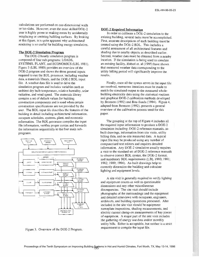
The DOE-2 Simulation Promam The DOE-2 hourly simulation program is

composed of four sub-programs: LOADS, SYSTEMS, PLANT, and ECONOMICS (LBL 198 1). Figure 3 (LBL 1980) provides an overview of the DOE-2 program and shows the three general inputs required to run the BDL processor, including weather data, a materials library, and the DOE-2 BDL input file. A weather data file is used to drive the simulation program and includes variables such as ambient dry bulb temperature, relative humidity, solar radiation, and wind speed. The materials library contains a set of default values for building construction components and is used when certain construction specifications are not provided by the user. The BDL input file describes the features of the building in detail including architectural information, occupant schedules, systems, plant, and economic information. The BDL processor compiles the input file information, verifies proper syntax and forwards the information sequentially to the four main sub- programs.

Figure 3. Overview of the DOE-2 Program.

DOE-2 Required Information In order to calibrate a DOE-2 simulation to the

existing building, several tasks must be accomplished. First, accurate descriptions of each building must be created using the DOE-2 BDL. This includes a careful assessment of all architectural features and shading due to nearby objects as described earlier. Second, weather data must be obtained from a nearby location. If the simulation is being used to simulate an existing facility, Haberl et, a1 (1995) have shown that measured weather data corresponding to the utility billing period will significantly improve the results.

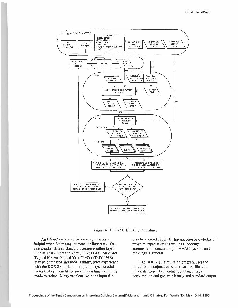
Finally, once all the syntax errors in the input file are resolved, numerous iterations must be made to match the simulated output to the measured whole- building electricity data using the statistical routines and graphical DOE-2 calibration methods developed by Bronson (1992) and Bou-Saada (1994). Figure 4, adapted from Bronson (1992). presents a general overview of the calibration process used for this paper.

The grouping at the top of Figure 4 includes all the required input information to produce a DOE-2 simulation including: DOE-2 reference manuals, as- built drawings, information from site visits, utility billing data, and on-site measured data. A typical input file may be produced using any number of computerized text editors and requires detailed information. Any DOE-2 simulation usually requires a visit to the standard set of DOE-2 reference manuals to observe correct BDL syntax, the DOE-2 format, and mandatory BDL requirements (LBL 1980; 1981 ; 1982; 1989; 1994). As-built drawings help to correctly dimension the building and calculate lighting and equipment levels.

A site visit is generally required to verify lighting and equipment counts as well as questionable dimensions and any other miscellaneous discrepancies. The site visit should include photographs of the surroundings and the equipment and detailed interviews with occupants, engineers, architects, and building operations personnel. Also included in the site visit should be equipment nameplate inspections, shading measurements, and electric current clamp-on measurements of key pieces of equipment. A major part of the site visit includes the gathering of energy use data and/or monthly utility bills. Either is acceptable, but neither is a strict requirement to compile the input file.

ESL-HH-96-05-23


DOE.2 EDITOR INPUT

I N P U T I N F O R M A T I O N SITE VISIT: - PHOTOGRAPHS

MEASURED WEATHER

ASUREMESTI UTILITY BILLS DATA

I

DOE-2.1 BUILDISO SIMULATIOS ( I-\-\ ) 4

HOURLY STABOARD OUTPUT OUTPUT REPORT REPORT

IFTP

FTP

- ST I> ILE A. JEDE T

- IDISTIFY AREAS WHERE THE DOES THE SIHULATED 1 MATCH SIMULATED THE MOXITORED DATA DO SOT DATA b o v DATA MATCH THE

MOSITORED DATA'

BATCH PROCESSISG

BUILDING BUlLDlSG

GRAPHICAL COYPARIS04 OF THE STATISTICAL CDMPARISOI OF SIMULATED COSSUMITIOS TO THE SIMULATED COIiSUMPTlOS

MONITORED CORSUMPTIOS TO MOWTORED COWSUMPTIOS

BUlLDlSG MODEL IS CALIBRATED TO YOSITORED BVILDISC COSSUYPTIOS

Figure 4. DOE-2 Calibration Procedure.

An HVAC system air balance report is also helpful when describing the zone air flow rates. On- site weather data or standard average weather tapes such as Test Reference Year (TRY) (TRY 1983) and Typical Meteorological Year (TMY) (TMY 1988) may be purchased and used. Finally, prior experience with the DOE-2 simulation program plays a crucial factor that can benefit the user in avoiding commonly made mistakes. Many problems with the input file

may be avoided simply by having prior knowledge of program expectations as well as a thorough engineering understanding of HVAC systems and buildings in general.

The DOE-2.1 E simulation program uses the input file in conjunction with a weather file and materials library to calculate building energy consumption and generate hourly and standard output

ESL-HH-96-05-23


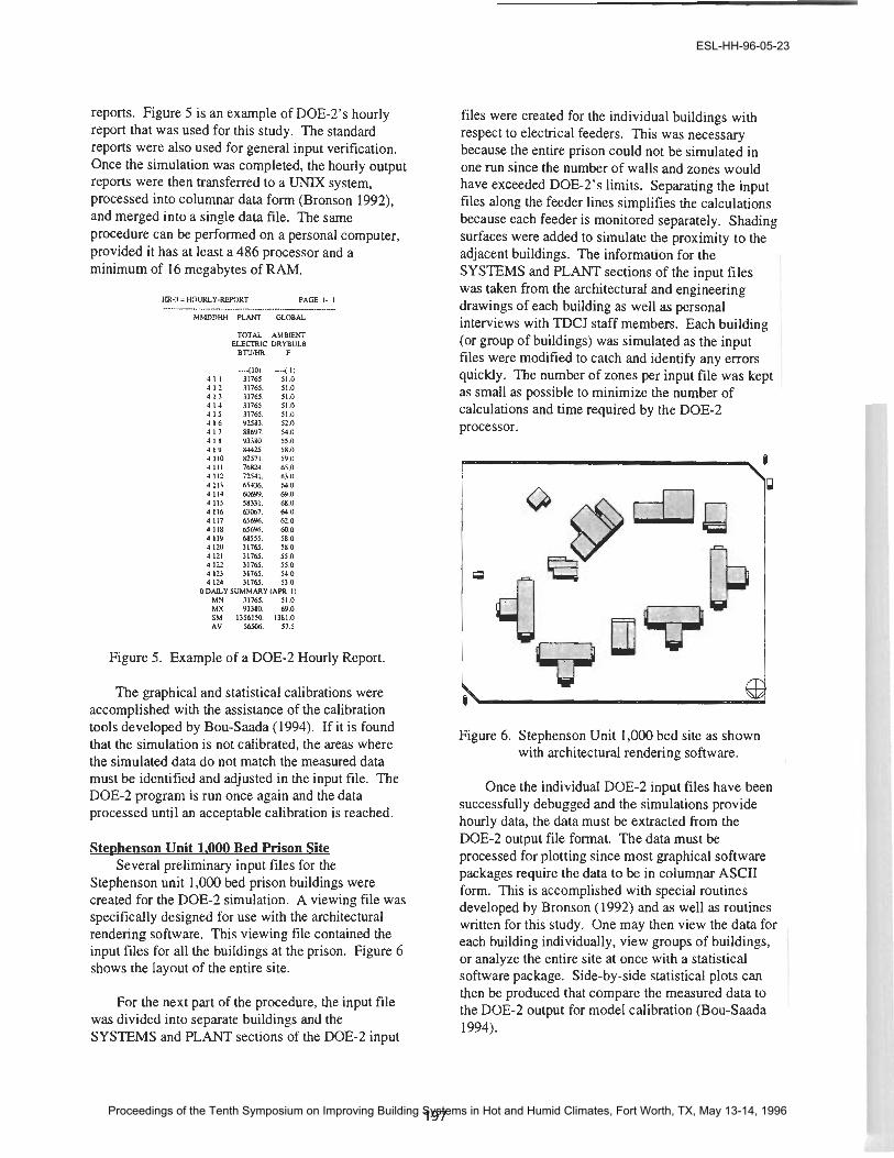
reports. Figure 5 is an example of DOE-2's hourly report that was used for this study. The standard reports were also used for general input verification. Once the simulation was completed, the hourly output reports were then transferred to a UNIX system, processed into columnar data form (Bronson 1992), and merged into a single data file. The same procedure can be performed on a personal computer, provided it has at least a 486 processor and a minimum of 16 megabytes of RAM.

HR-3 = HOURLY-REMJRT PAGE I - I

M M D D H H PLAKT GLOBAL

TOTAL AMBIENI ELECIRIC DRYBULB

BnJfHR F

4 113 65436. 61.0 4 I14 M6W. 6V.0 4 5 58331. 68.0 4 116 63067. 61.0 4 117 65696 62.0 4 llX 85696. a.0 4 llY 68555. 58 0 4 120 31765 511.0 4 121 31765. 55.0 4 122 31165. 55.0 4123 31765. Y.0 4 124 31765 53.0

ODAILY SUMMARY (APR I) MN 3176% 51.0 MX 93380. 69.0 SM 1356150. 1381.0 AV %SM. 57.5

Figure 5. Example of a DOE-2 Hourly Report.

The graphical and statistical calibrations were accomplished with the assistance of the calibration tools developed by Bou-Saada (1994). If it is found that the simulation is not calibrated, the areas where the simulated data do not match the measured data must be identified and adjusted in the input file. The DOE-2 program is run once again and the data processed until an acceptable calibration is reached.

Stephenson Unit 1.000 Bed Prison Site Several preliminary input files for the

Stephenson unit 1,000 bed prison buildings were created for the DOE-2 simulation. A viewing file was specifically designed for use with the architectural rendering software. This viewing file contained the input files for all the buildings at the prison. Figure 6 shows the layout of the entire site.

For the next part of the procedure, the input file was divided into separate buildings and the SYSTEMS and PLANT sections of the DOE-2 input

files were created for the individual buildings with respect to electrical feeders. This was necessary because the entire prison could not be simulated in one run since the number of walls and zones would have exceeded DOE-2's limits. Separating the input files along the feeder lines simplifies the calculations because each feeder is monitored separately. Shading surfaces were added to simulate the proximity to the adjacent buildings. The information for the SYSTEMS and PLANT sections of the input files was taken from the architectural and engineering drawings of each building as well as personal interviews with TDCJ staff members. Each building (or group of buildings) was simulated as the input files were modified to catch and identify any errors quickly. The number of zones per input file was kept as small as possible to minimize the number of calculations and time required by the DOE-2 processor.

Figure 6. Stephenson Unit 1,000 bed site as shown with architectural rendering software.

Once the individual DOE-2 input files have been successfully debugged and the simulations provide hourly data, the data must be extracted from the DOE-2 output file format. The data must be processed for plotting since most graphical software packages require the data to be in columnar ASCII form. This is accomplished with special routines developed by Bronson (1992) and as well as routines written for this study. One may then view the data for each building individually, view groups of buildings, or analyze the entire site at once with a statistical software package. Side-by-side statistical plots can then be produced that compare the measured data to the DOE-2 output for model calibration (Bou-Saada 1994).

ESL-HH-96-05-23


PHASE I1 Calibration Tools and Statistical Graphics

In order to improve the calibration procedures outlined by Bronson (1992) several new computer programs and graphical tools were developed, including modified routines originally created by Bronson (1992), Bou-Saada (1994), and Abbas (1993) as well as routines developed specifically for this paper. These improved calibration procedures include building architectural rendering (already introduced), new graphical methods (52-week box- whisker-mean plots, 24-hour daytype box-whisker- mean plots, binned box-whisker-mean plots), statistical goodness-of-fit calculations, and special processing routines for the building in question. These methods are discussed in the following sections.

Collect and Prepare Measured Data. Before DOE-2 is used to simulate an existing building, the user must consider how the model is to be validated. Various options are available varying in usefulness from monthly utility billing data, to short-term hourly end-use data from on-site monitoring, or even long-

Measured Whole Building Electricity

(a)

O' ro 30 r o i o ao -io l o 00 100 O Outside Air Temperature (F)

Measured Whole Building Electricity

0- 0 LO M 40 ¶4 8 0 7 0 M mO I W I10

Outside Air Temperature (F)

term hourly end-use data. The user may choose either to employ standard weather tapes such as TRY or TMY available from the National Climatic Data Center (NCDC) or to pack a site-specific weather tape for a more accurate weather dependent calibration (Haberl et al. 1995). Packing a TRY weather tape requires relative humidity, dry bulb temperature, global horizontal and beam solar radiation, and wind speed. Measured global horizontal data is converted into beam and diffuse data using the routines by Erbs et al. (1982).

For this project, the intention was to use on-site measured weather data to pack onto a TRY file. Unfortunately at the time of this writing, an ample amount of data was not available. Therefore, a TMY weather tape was used from nearby Kingsville, Texas. A TRY weather tape will be packed later for model tuning with the conclusion of Phase 11.

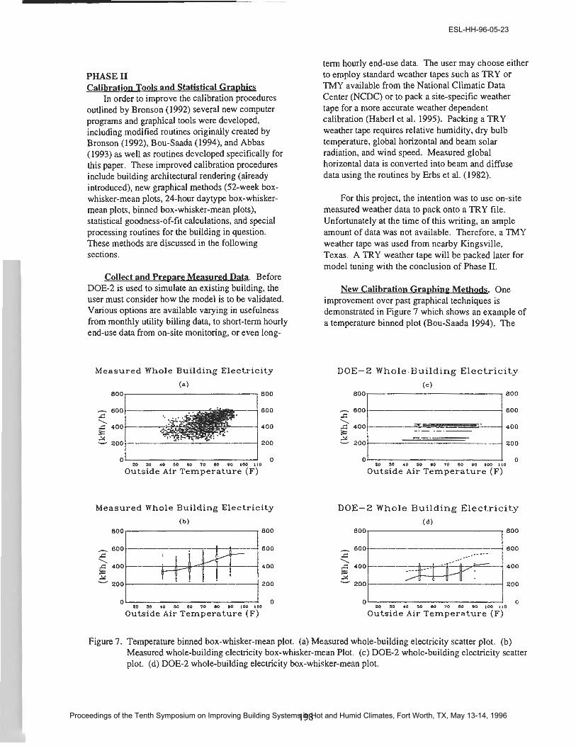
New Calibration G r a ~ h i n ~ Methods. One improvement over past graphical techniques is demonstrated in Figure 7 which shows an example of a temperature binned plot (Bou-Saada 1994). The

DOE-2 Whole. Building Electricity

0 0 0 20 30 40 50 80 70 10 90 I 0 0 110


DOE-2 Whole Building Electricity

0 1 0 20 LOO 40 )(I M 7 0 80 90 100 110


Figure 7. Temperature binned box-whisker-mean plot. (a) Measured whole-building electricity scatter plot. (b) Measured whole-building electricity box-whisker-mean Plot. (c) DOE-2 whole-building electricity scatter plot. (d) DOE-2 whole-building electricity box-whisker-mean plot.

ESL-HH-96-05-23


Temperatures < 45 F (a)

2 a00r-----7

5 0- 0 0 400 BOO 1200 1600 2000 2400

Time of Day

Temperatures < 45 F (b)

3 800

0- 0 0 400 800 1200 1600 2000 2400

Time of Day

Temperatures 45 F-75 F Icl

4 0- 0 0 400 BOO 1200 1600 2000 2400

Time of Day

Temperatures 45 F-75 F

0- 0 0 400 800 1200 1600 2000 2400

Time of Day

Temperatures > 75 F (el

n 800- 800 E

d O I 0 0 400 800 1200 1600 2000 2400

Time of Day

Temperatures > 75 F (1)

,,-____.,C_______~--.------ - 400 400

I . . W 200 0

200

d I o 0 0 400 800 1200 1600 2000 2400

Time of Day

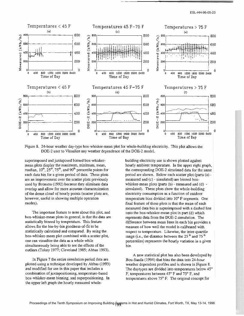
Figure 8. 24-hour weather day-type box-whisker-mean plot for whole-building electricity. This plot allows the DOE-2 user to Visualize any weather dependence of the DOE-2 model.

superimposed and juxtaposed binned box-whisker- mean plots display the maximum, minimum, mean, median, 10'. 25', 75', and 90' percentile points for each data bin for a given period of data. These plots are an improvement over the scatter plots previously used by Bronson (1992) because they eliminate data overlap and allow for more accurate characterization of the dense cloud of hourly points (scatter plots are, however, useful in showing multiple operation modes).

The important feature to note about this plot, and box-whisker-mean plots in general, is that the data are statistically binned by temperature. This feature allows for the bin-by-bin goodness-of-fit to be statistically calculated and compared. By using the box-whisker-mean plot combined with a scatter plot, one can visualize the data as a whole while simultaneously being able to see the effects of the outliers (Tukey 1977; Cleveland 1985; Abbas 1993).

In Figure 7 the entire simulation period data are plotted using a technique developed by Abbas (1993) and modified for use in this paper that includes a combination of juxtapositioning, temperature-based box-whisker-mean binning, and superpositioning. In the upper left graph the hourly measured whole-

building electricity use is shown plotted against hourly ambient temperature. In the upper right graph, the corresponding DOE-2 simulated data for the same period are shown. Below each scatter plot (parts (a) - measured and (c) - simulated) are binned box- whisker-mean plots (parts (b) - measured and (d) - simulated). These plots show the whole-building electricity consumption as a function of outdoor temperature bins divided into 10" F segments. One final feature of these plots is that the mean of each measured data bin is superimposed with a dashed line onto the box-whisker-mean plot in part (d) which represents data from the DOE-2 simulation. The difference between mean lines in each bin provides a measure of how well the model is calibrated with respect to temperature. Likewise, the inter-quartile range (i.e., the distance between the 25 ' and 75 ' percentiles) represents the hourly variation in a given bin.

A new statistical plot has also been developed by Bou-Saada (1994) that bins the data into 24-hour weather dependent profiles and is shown in Figure 8. The daytypes are divided into temperatures below 45" F, temperatures between 45" F and 75" F, and temperatures above 75" F. The original concept for

ESL-HH-96-05-23


this plot can be traced to the weather daytype analysis developed by Hadley (1993). The measured data are presented in parts (a). (c), and (e) and the simulated DOE-2 data are shown in parts (b), (d), and (f). These plots show that the buildings' 24-hour electricity profiles are influenced by the ambient temperature. The plots also provide a more efficient method of viewing the data based on heating only, no heating or cooling, and cooling only modes.

Figure 8 shows the data in a 24-hour box- whisker-mean format. This additional calibration procedure allows a DOE-2 user to view and analyze the weather dependent data on an hour-by-hour basis and adjust the hourly schedules in the input file accordingly. The solid line in parts (b), (d), and (f) is the simulated mean. The dashed line is the measured mean line from parts (a), (c), and (e) that is superimposed onto the simulated data so that hour- by-hour comparisons may be made.

One of the problems with presenting individual data points in an x-y plot (i.e.. hour-of-the-day versus kWh/h), is that it is difficult to judge the density of the data at a given point on the graph because the individual data points overlap. A particular problem with hourly simulated data is the overlap produced by weather independent scheduling such as lighting. As shown in Bou-Saada (1994) for hourly simulated data, a technique that can improve a graph which suffers from this problem is to jitter the individual data points by introducing a random noise into the variables used for the x or y axis (Cleveland 1985). This technique is useful for graphical presentation purposes that will be utilized during the calibration phase of this project not included with this paper.

An additional benefit to help finely tune a calibration is to analyze the outliers (i.e., the extra points on the outer bounds of the box-whisker-means seen in parts (d) and (f)). These points can help the DOE-2 user identify any problems with scheduling. In the initial simulation shown in Figure 8, for example, the outer limits represent points for a weekend or holiday which in the case of a prison is not correct. The user can in turn apply this useful iinformation to search through the input files for the incorrect schedule and take appropriate corrective measures.

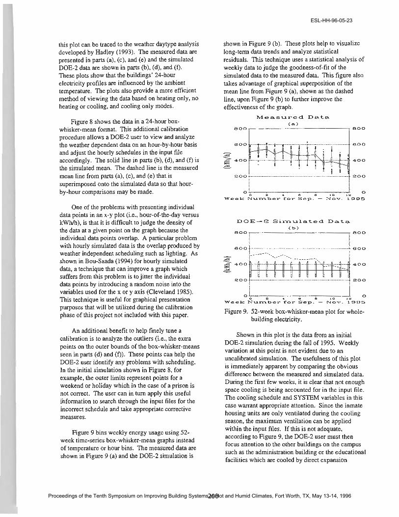
shown in Figure 9 (b). These plots help to visualize long-term data trends and analyze statistical residuals. This technique uses a statistical analysis of weekly data to judge the goodness-of-fit of the simulated data to the measured data. This figure also takes advantage of graphical superposition of the mean line from Figure 9 (a), shown as the dashed line, upon Figure 9 (b) to further improve the effectiveness of the graph.

M e a s u r e d D a t a

aoo,] "00

e a ro IZ W eek N u m b e r f o r Sep. - N o v . 1985

D O E - 2 Simulated D a t a <b)

soo, a00

2 4 0 0 1 0 1 2 0

Week N u m b e r f o r Sep. - N o v . 1 9 9 5

Figure 9. 52-week box-whisker-mean plot for whole- building electricity.

Shown in this plot is the data from an initial DOE-2 simulation during the fall of 1995. Weekly variation at this point is not evident due to an uncalibrated simulation. The usefulness of this plot is immediately apparent by comparing the obvious difference between the measured and simulated data. During the fust few weeks, it is clear that not enough space cooling is being accounted for in the input file. The cooling schedule and SYSTEM variables in this case warrant appropriate attention. Since the inmate housing units are only ventilated during the cooling season, the maximum ventilation can be applied within the input files. If this is not adequate.

Figure 9 bins weekly energy usage using 52- week time-series box-whisker-mean graphs instead according to Figure 9, the DOE-2 user must then

focus attention to the other buildings on the campus of temperature or hour bins. The measured data are shown in Figure 9 (a) and the DOE-2 simulation is

such as the administration building or the educational facilities which are cooled by direct expansion

ESL-HH-96-05-23


systems with several adjustments possible in the input files. In reality, several passes are required to tune the input files, particularly with a simulation of this scale due to the large number of buildings being simulated.

Due to the nature of this project with the number of loggers being present at the facility, the preceding plots have the flexibility of being of further help. Since there will be data from several feeders with no more than two buildings per feeder, the task of calibration is simplified. Each box-whisker-mean plot can be used to show data from the buildings that correspond to the respective feeders so that they may be compared to the measured data rather than relying only on total facility data as shown in the preceding statistical figures. The statistical approach described in the next section can then be used to numerically tabulate the results.

Calibration Calculation Methods. In a previous work, Bronson (1992) summed monthly simulation results and verified the calibration via a percent difference. Torres-Nunci (1989) and Hinchey (1 991) only declared the model "calibrated and submitted graphs to demonstrate the goodness-of-fit. Numerical differences only in the form o f f monthly differences were provided. Therefore, in the interest of furthering the calibration procedures, several statistical calculations can be used including a monthly mean difference, and hourly mean bias error (MBE) for each month, an hourly root mean squared error (RMSE) reported monthly, and an hourly coefficient of variation-root mean squared error (CV(RMSE)) (Kreider and Haberl 1994a; 1994b). These indices have proven useful in evaluating hourly models of building hourly use (Bou-Saada 1994). The values can then be tabulated for the total data as well as for each month. The statistical indices used to evaluate the models are defined below.

The percent difference is a simple calculation whereby a difference for each monthly measured and simulated energy consumption total is taken and divided by the measured monthly total consumption:

where: y is the predicted monthly value for the

building energy use,

ydaai is the measured monthly value for the building energy use, and

n is the number of months used in the simulation.

This index is the typical value reported for most DOE-2 predictions (Diamond and Hunn 198 1 ; Kaplan et al. 1990; Bronson 1992; McLain et al. 1993).

The mean bias error1, MBE (%) (Kreider and Haberl 1994a; 1994b), is a method used to determine a non-dimensional bias measure (sum of errors). between the simulated data and the measured data for each individual hour. The total difference. or sum of errors, between the predicted data and the simulated data is divided by the total number of hours considered in the calculation, thus rendering a mean bias. The p value, or number of regression parameters, was arbitrarily set to be zero. The result was then divided by the measured data mean to provide a non-dimensional value reported as a percentage. This calculation may be performed on any number of data points; however, it is convenient to show results as a function of monthly or total energy consumption.

where: - is the independent variable mean value of Ydl1a.i the data set corresponding to a particular

set of the dependent variables, n is the number of data points in the data

set, and P is the total number of regression

parameters in the model (which was assigned as 0 for the DOE-2 models).

The results of this calculation show that the MBE is actually the same as the percent difference calculation previously shown (Eq. 1). However, the true definition pertains to the bias, or error, of the mean difference value between the simulated data and the measured data.

Srinivm Katipamula, Ph.D. 1994. Personal Communicirtion, Richland, WA: Battelle Pacific Northwest Laboratory.

ESL-HH-96-05-23


The root mean squared error, RMSE (kWhIh), is found on an hourly basis by the following equation (SAS 1990):

where: the mean square error,

SSE MSE = , p=O and n-P

the sum of squares error,

yielding the equation:

The root mean squared error is typically referred to as a measure of variability, or how much spread exists in the data. For every hour, the error, or difference in paired data points is calculated and squared. The sum of squares errors (SSE) are then added for each month and for the total periods and divided by their respective number of points yielding the MSE; whether for each month or the total period. A square root of the result is then reported as the root mean squared error.

The coefficient of variation-root mean squared error, CV(RMSE) (96) (Draper and Smith 1981) is essentially the root mean squared error divided by the measured mean:

where:

It is often convenient to report a non-dimensional result. CV(RMSE) allows one to determine how well a model fits the data; the lower the CV(RMSE), the better the calibration (the model in this case is the

DOE-2 predicted data). Therefore, a CV(RMSE) is calculated for hourly data and presented on both a monthly summary and total data period.

The purpose of calculating the CV(RMSE) and comparing the results with the standard percent difference calculation is to demonstrate that a percent difference report may be misleading. Since the percent difference calculations are usually shown for total monthly simulations or even total simulation data periods, the reader is never certain if the model is a true representation of the actual building or if the f errors have canceled out. If one examines the hour- by-hour data results, it would be evident that each pair of points would in all likelihood be dissimilar and in some cases be significantly different, despite using measured weather data to drive the simulation model. Reporting monthly data therefore does not take into account the canceling out of individual differences observed when the simulation over- predicts during one hour and under-predicts during the next hour by approximately the same amount.

SUMMARY This paper has investigated techniques for

calibrating computer building energy simulation methods for large institutions and has presented several new techniques for improved calibration. A multiple building state correctional institute case study site was simulated with DOE-2.1E using hourly measured whole-building electricity data to demonstrate the new techniques. The methodology incorporated the simulation of several buildings simultaneously by modeling the buildings as zones rather than as individual buildings due to simulation software limitations. Data processing routines were developed for processing large amounts of DOE-2 hourly data from all the buildings which were then compared to hourly measured electricity data.

Several improved calibration approaches were presented which included architectural rendering for architectural layout verification and presentation, graphical procedures for visualizing the calibration accuracy, and statistical goodness-of-fit parameters for quantitatively comparing simulated data to measured data. The graphs shown in this paper comparing the simulated data to the measured data represent the simulation results after the first uncalibrated DOE-2 pass. By concurrently using all the techniques demonstrated here the model can be further refined in order to accurately portray the site thus improving prior calibration techniques. This reduces the modeling time as well as some of the

ESL-HH-96-05-23


uncertainties that undoubtedly arise with computer simulations. It is also quite clear from the graphical methods used in this paper that calibrating a model to measured data is invaluable versus the sole reliance on architectural plan data.

ACKNOWLEDGEMENTS Work discussed in this paper was sponsored by

the Texas Department of Criminal Justice under contract number C95-259. We deeply appreciate all those involved for their contributions including Linn Hutchins, Frank Lloyd Jr., and Norm Pleasant of the TDCJ, and Bryce Munger of the Energy Systems Laboratory.

REFERENCES

Abbas, M. 1993. "Development of Graphical Indices for Building Energy Data", M.S. Thesis, Texas A&M University, College Station, TX, Energy Systems Laboratory Report No. ESL-TH-93/12-02.

Bou-Saada, T.E. 1994. "An Improved Procedure for Developing a Calibrated Hourly Simulation Model of an Electrically Heated and Cooled Commercial Building", M.S. Thesis, Energy Systems Laboratory Report No. ESL-TH-94/12-01, Texas A&M University, College Station, TX.

Bou-Saada, T.E. and Haberl, J.S. 1995a. "An Improved Procedure for Developing Calibrated Hourly Simulation Models." Building Simulation '95, Fourth International Conference Proceedings, International Building Performance Simulation Association, pp. 475-484. Energy Systems Laboratory Report No. ESL-PA-95/08-01, Texas A&M University, College Station, TX.

Bou-Saada, T.E. and Haberl, J.S. 1995b. "A Weather Daytyping Procedure for Disaggregating Hourly End- use Loads in an Electrically Heated and Cooled Building from Whole-building Hourly Data." Proceedings of the 30th Intersocietv Enerov Conversion En~ineerine Conference, Jul. 30 - Aug. 4, Vol. 2, pp. 349-355. Energy Systems Laboratory Report No. ESL-PA-95107-0 1, Texas A&M University, College Station, TX.

Cleveland. W.S. 1985. "The Elements of Graphing Data", Wadsworth & Brooks/Cole, Pacific Grove. CA.

Diamond, S.C. and B.D. Hunn. 1981. "Comparison of DOE-2 Computer Program Simulations to Metered Data for Seven Commercial Buildings." ASHRAE Transactions, Vol. 87, No. 1, p. 1222 - 123 1.

Draper, N. and H. Smith. 1981. "Applied Regression Analysis", 2nd. Ed., John Wiley & Sons, New York, NY.

Erbs, D.G., S.A. Klein and J.A. Duffle. 1982. "Estimation of diffuse radiation fraction for hourly, daily, and monthly-average global radiation." Solar Energy, Vol. 28, NO. 4, pp. 293-302.

Haberl, J.S., J.D. Bronson, and D.L. O'Neal. 1995. "Impact of using measured weather data versus TMY weather data in a DOE-2 simulation." ASHRAE Transactions, Vol. 101, No. 2. ESL Report No. ESL- TR-93/09-02. College Station, TX.

Hadley, D.L. 1993. "Daily Variation in HVAC System Electrical Energy Consumption in Response to Different Weather Conditions." Enerev and Buildines, Vol. 19, p. 235 - 247.

Hinchey, S.B. 199 1. "Influence of Thermal Zone Assumptions on DOE-2 Energy Use Estimations of a Commercial Building", M.S. Thesis, Texas A&M University, College Station, TX., Energy Systems Laboratory Report No. ESL-TH-9 1/09-06.

Kaplan, M.B., B. Jones, and J. Jansen. 1990. "DOE- 2.1C Model Calibration with Monitored End-use Data." Proceedines from the ACEEE 1990 Summer Studv on Energv Effkiencv in Buildings, Washington, DC: American Council for an Energy Efficient Economy. Vol. 10, p. 10.1 15 - 10.125.

Kreider J.F. and J.S. Haberl. 1994a. "Predicting Hourly Building Energy Use: The Great Energy Predictor Shootout - Overview and Discussion of Results." ASHRAE Transactions, Vol. 100, No. 2.

Kreider J.F. and J.S. Haberl. 1994b. "Predicting

Bronson, J.D. 1992. "Calibrating DOE-2 to Weather Hourly Building Energy Usage." ASHRAE ~ o u i a l ,

and Non-weather Dependent Loads for a Commercial Vol. 36, p. 72 - 81.

Building", M.S. Thesis, Energy Systems Laboratory Report No. ESL-TH-92/04-01, Texas A&M LBL. 1980. "DOE-2 User Guide. Ver. 2.1 .". University, College Station, TX. Lawrence Berkeley Laboratory and Los Alamos

National Laboratory, LBL Report No. LBL-8689

ESL-HH-96-05-23


Rev. 2; DOE-2 User Coordination Office, LBL. Berkeley, CA.

LBL. 1981. "DOE-2 Engineers Manual, Ver. 2.1A", Lawrence Berkeley Laboratory and Los Alamos National Laboratory, LBL Report No. LBL-11353; DOE-2 User Coordination Office, LBL, Berkeley, CA.

LBL. 1982. "DOE-2.1 Reference Manual Rev. 2.1 A", Lawrence Berkeley Laboratory and Los Alarnos National Laboratory, LBL Report No. LBL- 8706 Rev. 2; DOE-2 User Coordination Office, LBL, Berkeley, CA.

LBL. 1989. "DOE-2 Supplement, Ver 2.1D. Lawrence Berkeley Laboratory, LBL Report No. LBL-8706 Rev. 5 Supplement. DOE-2 User Coordination Office, LBL, Berkeley, CA.

LBL. 1994. "DOE-2 Basics, Version 2. l E , Lawrence Berkeley Laboratory, LBL Report No. LBL-35520. DOE-2 User Coordination Office, LBL, Berkeley, CA.

McLain, H.A., S.B. Leigh, and J.M. MacDonald. 1993. "Analysis of Savings Due to Multiple Energy Retrofits in a Large Office Building", Oak Ridge National Laboratory, OFWL Report No. ORNLICON-363, Oak Ridge, TN.

SAS Institute, Inc. 1990. "SASISTAT User's Guide", Cary, NC, Ver. 6,4th ed., Vol. 2.

Torres-Nunci, N. 1989. "Simulation Modeling Energy Consumption in the Zachry Engineering Center", Master's Project Report, Texas A&M University, College Station, TX.

TRY. 1983. "Test Reference Year (TRY) Tape Reference Manual - TD-9706", National Climatic Data Center, Asheville, NC.

TMY. 1988. "Typical Meteorological Year User's Manual - TD-9734", National Climatic Data Center, Asheville, NC.

Tukey, J.W. 1977. "Exploratory Data Analysis", Addison-Wesley Publishing Co., Reading. MA.

ESL-HH-96-05-23


Documents

COMPUTER ENERGY MODELING TECHNIQUES FOR SIMULATING …