Modeling and motion control of a hybrid-driven underwater glider

Khalid Isa &M. R. Arshad

Underwater Robotics Research Group (URRG), School of Electrical and Electronic Engineering,

Engineering Campus, Universiti Sains Malaysia (USM), 14300 Nibong Tebal, Pulau Pinang,

Malaysia.

[Email: halid@uthm.edu.my and rizal@eng.usm.my]

Received ; revised

Present study consists a mathematical model and motion control analysis for a hybrid-driven

underwater glider, which can be propelled by using buoyancy and propeller with an addition of wings

and a rudder that can be controlled independently. Thus, it can overcome the constraints of speed and

maneuverability that was normally possessed by the fixed-winged buoyancy-driven underwater glider.

Mathematical model of the glider is based on the Newton-Euler approach, and the hydrodynamics of

the glider are estimated based on the Slender-body theory. Glider is controlled by six control inputs:

the deflection angle of the right and left wing, the angle of a rudder, two net forces of a sliding mass

and the pumping rate of a ballast pump. A Linear Quadratic Regulator (LQR) controller is used to

obtain better control performance over the glider motion. Results show that the glider is stable, and

the controller performance is satisfactory.

[Keywords: Underwater glider, Modeling, Motion control, LQR]

Introduction

The hybrid-driven underwater glider is a new class and practical underwater platform which can be a

powerful tool for oceanographic sensing and sampling. The hybrid-driven glider combines the

attributes of the buoyancy-driven underwater glider and conventional autonomous underwater vehicle

(AUV). The development of this glider able to overcome the weaknesses of the conventional glider.

The conventional underwater gliders such as the legacy underwater glider1-4

are fixed-winged

buoyancy-driven underwater gliders, which have already demonstrated highly energy efficient.

However, these gliders have limitations in terms of speed and maneuverability due to the absence of a

propeller and limited external control surfaces such as controllable wings and a controllable rudder.

Thus, in order to increase the efficiency of the conventional glider such as the speed and

maneuverability, the hybrid-driven underwater glider has been designed by having wings and a rudder

that can be controlled independently and can be propelled by using buoyancy and propeller system.

The research works on the hybrid-driven underwater glider, as well as, the underwater glider with

independently controllable wings were carried out by several researchers5-7. However, the glider

design and configuration that was simulated by these researchers were different from our design.

Some of them has fixed wings and a controllable rudder5, and some of them has no wings6. Other than

that, there was a work that presented a buoyancy-driven underwater glider with controllable wings7.

Various control methods have been proposed to control underwater vehicles, whether through

simulation or actual experiment8-9

. In terms of the glider controller, most of the existing gliders have

used simple PID10-11

, and LQR12-14

controller to control the glider motion and attitude, and the

performance comparison between PID and LQR for the glider control has been analyzed by Noh,

Arshad and Mokhtar15

. However, these control systems are implemented for the Single-Input-Single-

Output (SISO) system, and the presence of disturbance is neglected. Since, the hybrid-driven

underwater glider has six control inputs; therefore, the motion control system is based on the

Multiple-Input-Multiple-Output (MIMO) system and the LQR controller is used to control the glider

motion. In addition, the presence of disturbance from the water currents has been taken into account.

This paper explains the mathematical model and motion control of the hybrid-driven underwater

glider. Hybrid-driven underwater glider in this work is an extension of the buoyancy-driven

underwater glider and propeller-driven underwater glider presented in Isa and Arshad16-17. Present

study is an attempt to analyze the motion control of the glider by using the LQR controller and to

compare the LQR performance between the glider motion with disturbance and without disturbance.

Materials and Methods

This section discusses the glider structure, mathematical model and equations of motion of the glider,

and the hydrodynamics forces. In this work, the model derivation presented by Fossen18-19 and

Graver20

is used as a basis for modeling the hybrid-driven autonomous underwater glider.

The USM hybrid-driven underwater glider has been modeled by using the Newtonian theory and the

glider hydrodynamics have been analytically estimated based on the Strip theory approach21

. Glider is

divided into two structures: the external structure and internal structure. On one hand, the external

structure is divided of two areas: the wing-body area and tail area. Wing-body area is composed of

independently controllable wings, a cylindrical hull and a nose. Meanwhile, the tail area has

horizontal wings/fins, a controllable rudder and a propeller. On the other hand, the internal structure

of the glider is composed of a ballast pump, a sliding mass, batteries, and electronics components such

as the acoustic sensor, accelerometer, data logger and microcontroller. Figure 1 and 2 show the glider

structure and configuration, respectively.

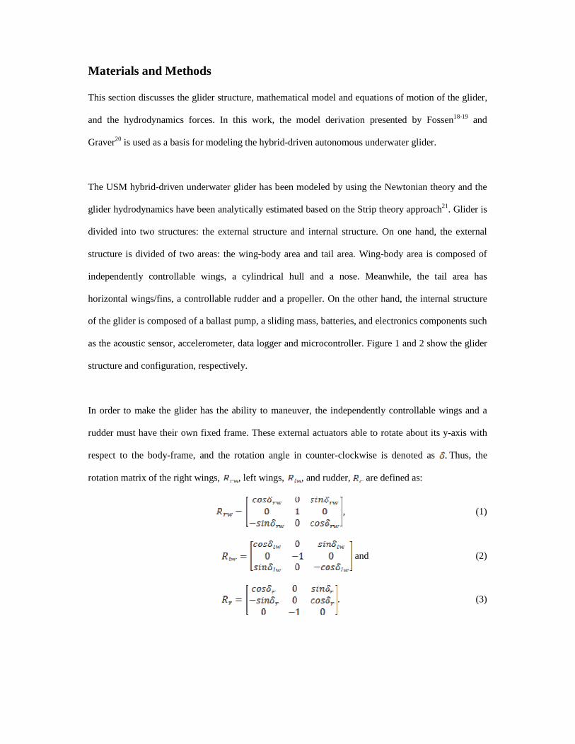
In order to make the glider has the ability to maneuver, the independently controllable wings and a

rudder must have their own fixed frame. These external actuators able to rotate about its y-axis with

respect to the body-frame, and the rotation angle in counter-clockwise is denoted as Thus, the

rotation matrix of the right wings, , left wings, , and rudder, are defined as:

, (1)

and (2)

. (3)

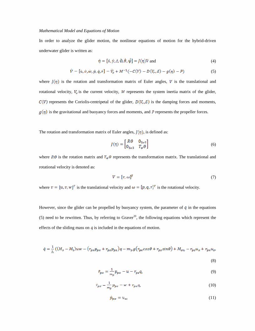
Mathematical Model and Equations of Motion

In order to analyze the glider motion, the nonlinear equations of motion for the hybrid-driven

underwater glider is written as:

and (4)

(5)

where is the rotation and transformation matrix of Euler angles, is the translational and

rotational velocity, is the current velocity, represents the system inertia matrix of the glider,

represents the Coriolis-centripetal of the glider, is the damping forces and moments,

is the gravitational and buoyancy forces and moments, and represents the propeller forces.

The rotation and transformation matrix of Euler angles, , is defined as:

(6)

where is the rotation matrix and represents the transformation matrix. The translational and

rotational velocity is denoted as:

(7)

where is the translational velocity and is the rotational velocity.

However, since the glider can be propelled by buoyancy system, the parameter of in the equations

(5) need to be rewritten. Thus, by referring to Graver20, the following equations which represent the

effects of the sliding mass on is included in the equations of motion.

,

(8)

, (9)

, (10)

, (11)

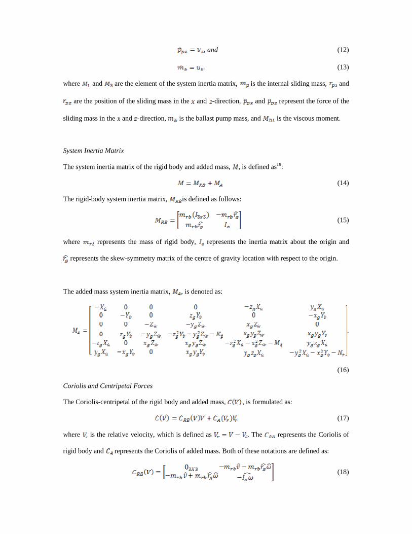
, and (12)

. (13)

where and are the element of the system inertia matrix, is the internal sliding mass, and

are the position of the sliding mass in the and -direction, and represent the force of the

sliding mass in the and -direction, is the ballast pump mass, and is the viscous moment.

System Inertia Matrix

The system inertia matrix of the rigid body and added mass, , is defined as18

:

(14)

The rigid-body system inertia matrix, is defined as follows:

(15)

where represents the mass of rigid body, represents the inertia matrix about the origin and

represents the skew-symmetry matrix of the centre of gravity location with respect to the origin.

The added mass system inertia matrix, , is denoted as:

.

(16)

Coriolis and Centripetal Forces

The Coriolis-centripetal of the rigid body and added mass, , is formulated as:

(17)

where is the relative velocity, which is defined as . The represents the Coriolis of

rigid body and represents the Coriolis of added mass. Both of these notations are defined as:

(18)

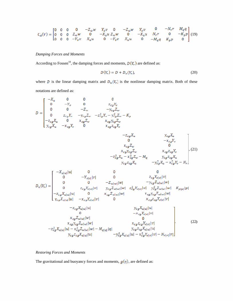
(19)

Damping Forces and Moments

According to Fossen18

, the damping forces and moments, are defined as:

, (20)

where is the linear damping matrix and is the nonlinear damping matrix. Both of these

notations are defined as:

, (21)

. (22)

Restoring Forces and Moments

The gravitational and buoyancy forces and moments, , are defined as:

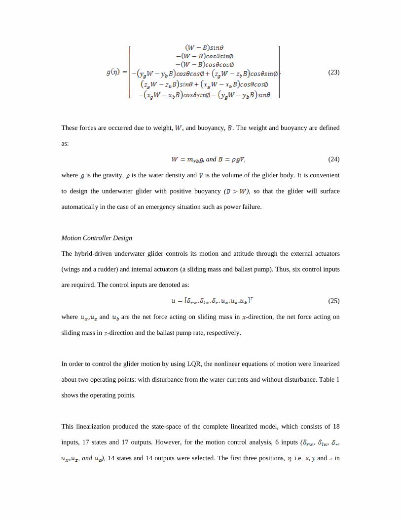
(23)

These forces are occurred due to weight, , and buoyancy, . The weight and buoyancy are defined

as:

, and (24)

where is the gravity, is the water density and is the volume of the glider body. It is convenient

to design the underwater glider with positive buoyancy ( ), so that the glider will surface

automatically in the case of an emergency situation such as power failure.

Motion Controller Design

The hybrid-driven underwater glider controls its motion and attitude through the external actuators

(wings and a rudder) and internal actuators (a sliding mass and ballast pump). Thus, six control inputs

are required. The control inputs are denoted as:

(25)

where and are the net force acting on sliding mass in -direction, the net force acting on

sliding mass in -direction and the ballast pump rate, respectively.

In order to control the glider motion by using LQR, the nonlinear equations of motion were linearized

about two operating points: with disturbance from the water currents and without disturbance. Table 1

shows the operating points.

This linearization produced the state-space of the complete linearized model, which consists of 18

inputs, 17 states and 17 outputs. However, for the motion control analysis, 6 inputs ( , , ,

, and ), 14 states and 14 outputs were selected. The first three positions, i.e. and in

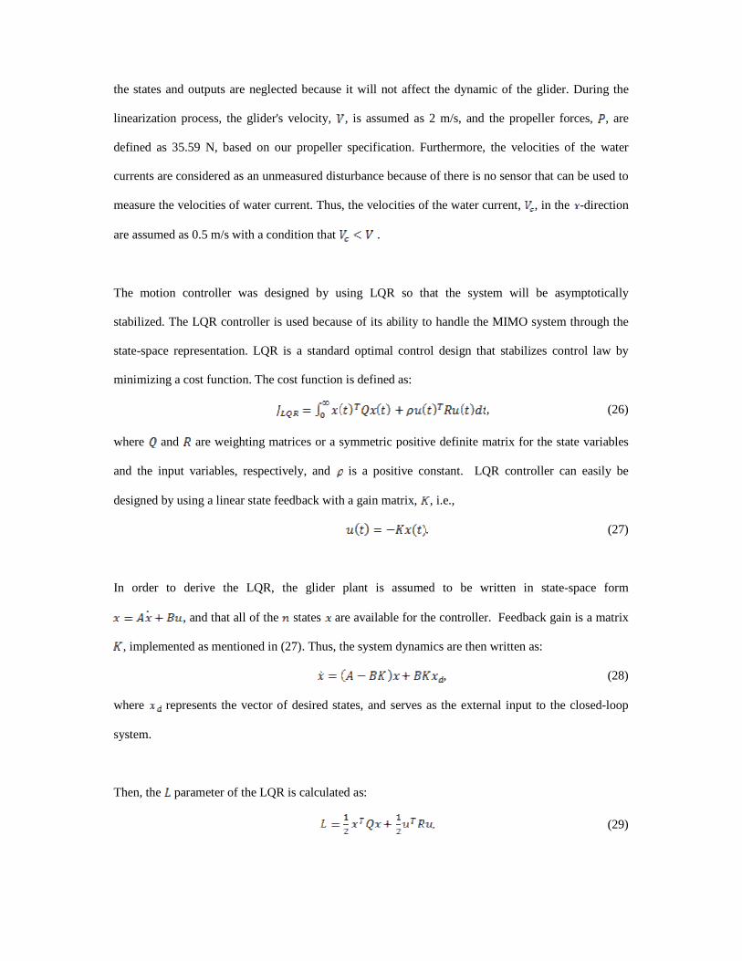
the states and outputs are neglected because it will not affect the dynamic of the glider. During the

linearization process, the glider's velocity, , is assumed as 2 m/s, and the propeller forces, , are

defined as 35.59 N, based on our propeller specification. Furthermore, the velocities of the water

currents are considered as an unmeasured disturbance because of there is no sensor that can be used to

measure the velocities of water current. Thus, the velocities of the water current, , in the -direction

are assumed as 0.5 m/s with a condition that .

The motion controller was designed by using LQR so that the system will be asymptotically

stabilized. The LQR controller is used because of its ability to handle the MIMO system through the

state-space representation. LQR is a standard optimal control design that stabilizes control law by

minimizing a cost function. The cost function is defined as:

, (26)

where and are weighting matrices or a symmetric positive definite matrix for the state variables

and the input variables, respectively, and is a positive constant. LQR controller can easily be

designed by using a linear state feedback with a gain matrix, , i.e.,

. (27)

In order to derive the LQR, the glider plant is assumed to be written in state-space form

, and that all of the states are available for the controller. Feedback gain is a matrix

, implemented as mentioned in (27). Thus, the system dynamics are then written as:

, (28)

where represents the vector of desired states, and serves as the external input to the closed-loop

system.

Then, the parameter of the LQR is calculated as:

(29)

where the requirement that implies that both and are positive definite. Thus, in the case of

linerized plant dynamics, the , , , and , so that

, (30)

, (31)

, = 0, and (32)

= 0. (33)

By defining , where can be found by solving the continuous time Riccati differential

equation, and inserting this into the equation (32), and then using the equation (30), and a substitution

for , the following matrix Riccati equation is obtained as:

. (34)

Thus, the steady-state of LQR is defined as:

. (35)

and then is derived from using the following equation:

(36)

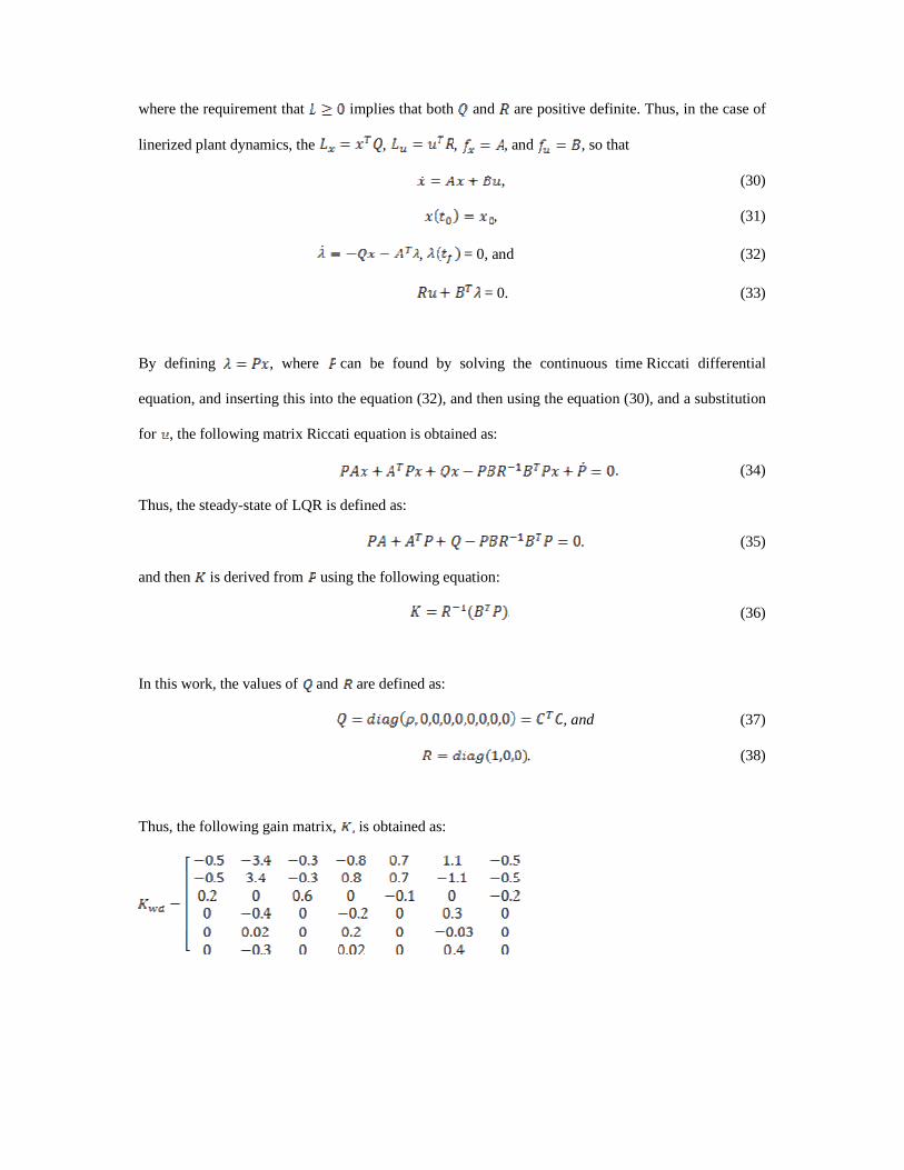
In this work, the values of and are defined as:

, and (37)

. (38)

Thus, the following gain matrix, is obtained as:

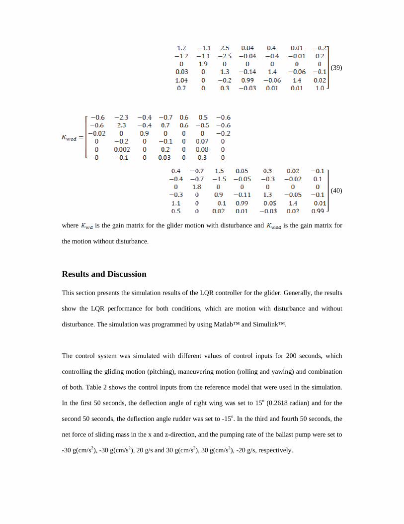
(39)

(40)

where is the gain matrix for the glider motion with disturbance and is the gain matrix for

the motion without disturbance.

Results and Discussion

This section presents the simulation results of the LQR controller for the glider. Generally, the results

show the LQR performance for both conditions, which are motion with disturbance and without

disturbance. The simulation was programmed by using Matlab™ and Simulink™.

The control system was simulated with different values of control inputs for 200 seconds, which

controlling the gliding motion (pitching), maneuvering motion (rolling and yawing) and combination

of both. Table 2 shows the control inputs from the reference model that were used in the simulation.

In the first 50 seconds, the deflection angle of right wing was set to 15o (0.2618 radian) and for the

second 50 seconds, the deflection angle rudder was set to -15o. In the third and fourth 50 seconds, the

net force of sliding mass in the x and z-direction, and the pumping rate of the ballast pump were set to

-30 g(cm/s2), -30 g(cm/s2), 20 g/s and 30 g(cm/s2), 30 g(cm/s2), -20 g/s, respectively.

Figures 3-6 show the glider motion and attitude that was controlled by the LQR controller based on

the control inputs in Table 2. Motion that are depicted in the figures are rolling, yawing, downward

and upward motion. In addition, a comparison between the performance of LQR controller with

disturbance and without disturbance is also presented.

Figure 3 shows the feedback of the LQR controller for both conditions. The graph has shown that,

after 100 seconds, the roll and yaw angle were not affected by the different values of the sliding mass

net force and ballast pump rate. Although the difference between the performance of the LQR with

disturbance and without disturbance was obvious, the LQR able to compensate the disturbance from

the water current and stabilized the glider.

Figure 4 presents the LQR feedback of the translational velocities namely the surge, , sway, , and

heave, . The graph has shown that the controller response of surge velocity for both conditions was

quite similar, but the settling time for the LQR with disturbance was faster than the LQR without

disturbance. On the other hand, there was a big gap between the response of the sway and heave for

both conditions.

The LQR response of the rotational velocities namely the roll rate, , pitch rate, , and yaw rate, , is

shown in Figure 5. The graph has shown that the feedback response of the roll and yaw rate for both

conditions had a similar response and settling time. However, the response of the pitch rate for both

conditions was difference due to the presence of disturbance that affected the pitch angle of the glider.

Figure 6 shows the feedback response of the sliding mass and ballast pump for both conditions. The

position of the sliding mass in -direction was affected by the presence of the disturbance from the

water current velocity. This is because the sliding mass controls the pitch angle of the glider.

However, the sliding mass force and the ballast mass converged to the desired sliding mass net force

and ballast mass rate.

In summary, the amplitude values of the outputs that were obtained from the LQR feedback are

tabulated in Table 3. In addition, the error of the LQR feedback between motion with disturbance and

without disturbance is presented in Table 4. Data in this table shows that the LQR feedback of the

pitch rate has produced the highest average of error rate with a value of 11.2267 for 200 seconds of

simulation. On other hand, the yaw rate has produced the lowest average of error with a value of 0.

Conclusion

In conclusion, this paper presents the mathematical model and motion control of the hybrid-driven

underwater glider. The objectives of this paper are to analyze the motion control of the glider by using

the LQR controller and to compare the LQR performance between the glider motion with disturbance

and without disturbance. Due to that, the nonlinear glider model has been designed and linearized at

two operating points, where the presence of water current velocity as a disturbance was included in

one of the operating points. The simulation was programmed by using Matlab™ and Simulink™.

Several values of control inputs have been tested, and the simulations demonstrated that the results are

acceptable, and the stability of the glider has been gained by the LQR for the motion with disturbance

and without disturbance. However, the feedback responses for both conditions had glitches. Due to

that, a biologically inspired control algorithm has been designing to overcome the drawbacks of the

motion controller of the glider.

Acknowledgment

The author would like to thank the Malaysia Ministry of Higher Education (MOHE), ERGS-

203/PELECT/6730045, Universiti Sains Malaysia (USM) and Universiti Tun Hussein Onn Malaysia

(UTHM) for supporting the research.

References

1. Webb, D.C., Simonetti, P.J., Jones, C.P., SLOCUM: An underwater glider propelled by

environment energy, IEEE Journal of Oceanic Engineering, 26 (4) (2001) 447-452.

2. Sherman, J., Davis, R.E., Owens, W.B., Valdes, J., The autonomous underwater glider "Spray".

IEEE Journal of Oceanic Engineering, 26 (4) (2001) 437-446.

3. Eriksen, C.C., Osse, T.J., Light, R.D., Wen, T., Lehman, T.W., Sabin, P.L., Ballard, J.W.,

Chiodi, A.M., Seaglider: A long range autonomous underwater vehicle for oceanographic

research, IEEE Journal of Oceanic Engineering, 26 (4) (2001) 424-436.

4. Osse, T.J. Eriksen, C.C, The deepglider: a full ocean depth glider for oceanographic research,

(IEEE Ocean), 2007, pp. 1-12.

5. Shu-Xin, W., Xiu-jun, S., Yan-hui, W., Jian-guo, W., Xiao-Ming. W., Dynamic Modeling and

Simulation for a Winged Hybrid-Driven Underwater Glider. China Ocean Engineering 25(1)

(2011) 97-112.

6. Caiti, A., and Calabro, V., Control-oriented modeling of a hybrid AUV, (Proceedings of the

IEEE Int. Conf. on Robotics and Automation), 2010, pp. 5275-5280.

7. Arima, M., Ichihashi, N., and Miwa, Y., Modelling and Motion Simulation of an Underwater

Glider with Independently Controllable Main Wings, (Oceans 2009-Europe), 2009, pp. 1 - 6.

8. Budiyono, A., Advances in unmanned underwater vehicles technologies : Modeling , control

and guidance perspectives. Indian Journal of Geo-Marine Sciences, 38(3) (2009) 282–295.

9. Yuh, J., Design and Control of Autonomous Underwater Robots: A Survey. Autonomous

Robots, 8(1) (2000), 7–24.

10. Bachmayer, R., Graver, J.G., Leonard, N.E., Glider control: a close look into the current glider

controller structure and future developments, (Proceedings of OCEANS 2003, IEEE Press),

2003, pp. 951-954.

11. Mahmoudian, N. and Woolsey, C., Underwater glider motion control, (Proceedings of the 47th

IEEE Conference on Decision and Control), 2008, pp 552-557.

12. Leonard, N.E., Graver, J.G., Model based feedback control of autonomous underwater gliders,

IEEE Journal of Oceanic Engineering, 26(4) (2001) 633-645.

13. Lei, K., Yuwen, Z., Hui, Y., Zhikun, C., MATLAB-based simulation of buoyancy-driven

underwater glider motion, Journal Ocean University of China, 7(1) (2008) 133 - 188.

14. Wang, Y., Zhang, H., Wang, S., Trajectory control strategies for the underwater glider,

(Proceedings of International Conference on Measuring Technology and Mechatronics

Automation, IEEE Press), 2009, pp. 918-921.

15. Noh, M.M., Arshad, M.R., Mokhtar, R.M., Depth and pitch control of USM underwater glider:

performance comaprison PID vs. LQR, Indian Journal of Geo-Marine Sciences, 40(2) (2011)

200-206.

16. Isa, K., Arshad, M.R., Buoyancy-driven underwater glider modelling and analysis of motion

control, Indian Journal of Geo-Marine Sciences, 41(6) (2012) 516-526.

17. Isa, K., Arshad, M.R., Propeller-Driven Underwater Glider Modelling and Motion Control,

International Journal of Imaging and Robotics, 10(2) (2013) 86-104.

18. Fossen, T.I, Marine control systems: guidance, navigation and control of ships, rigs and

underwater vehicles, (Marine Cybernatics), 2002, pp. 569.

19. Fossen, T.I., Handbook of marine craft hydrodynamics and motion control, (John Wiley &

Sons), 2011, pp. 596.

20. Graver, J.G., Underwater gliders: dynamics, control and design, Ph.D. Thesis, Princeton

University, 2005, pp. 273.

21. Isa, K., Arshad, M.R., Dynamic modeling and characteristics estimation for USM underwater

Glider, (Proceedings of IEEE Control and System Graduate Research Colloquium (ICSGRC)

Incorporating The International Conference on System Engineering and Technology (ICSET)),

2011, pp. 12-17.

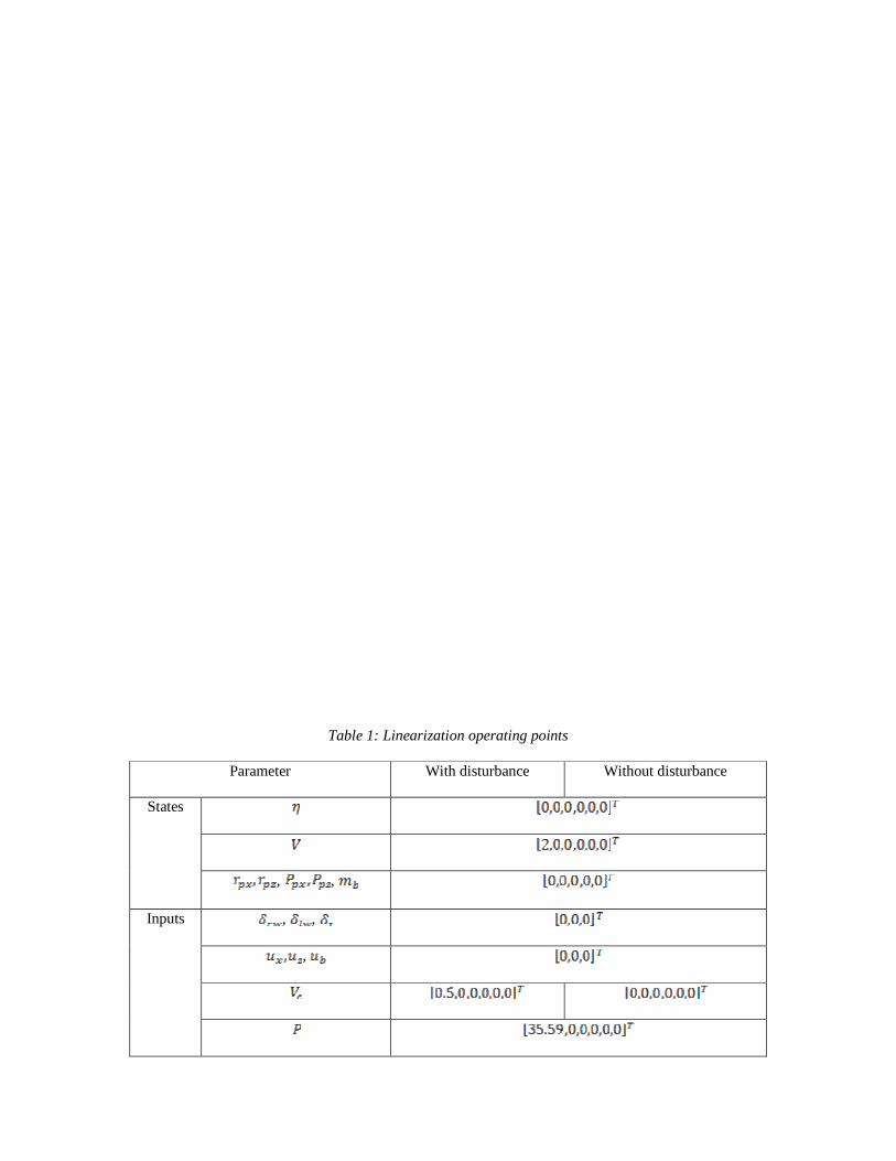
Table 1: Linearization operating points

Parameter With disturbance Without disturbance

States

, ,

, ,

,

Inputs

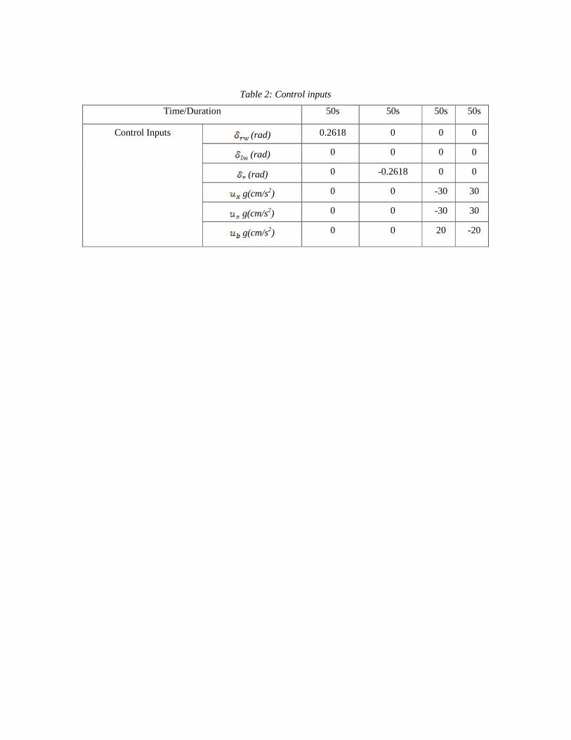
Table 2: Control inputs

Time/Duration 50s 50s 50s 50s

(rad) 0.2618 0 0 0

(rad) 0 0 0 0

(rad) 0 -0.2618 0 0

g(cm/s2) 0 0 -30 30

g(cm/s2) 0 0 -30 30

Control Inputs

g(cm/s2) 0 0 20 -20

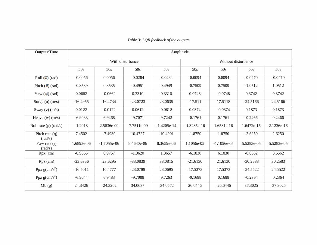
Table 3: LQR feedback of the outputs

Amplitude

With disturbance Without disturbance

Outputs\Time

50s 50s 50s 50s 50s 50s 50s 50s

Roll ( ) (rad) -0.0056 0.0056 -0.0284 -0.0284 -0.0094 0.0094 -0.0470 -0.0470

Pitch ( ) (rad) -0.3539 0.3535 -0.4951 0.4949 -0.7509 0.7509 -1.0512 1.0512

Yaw ( ) (rad) 0.0662 -0.0662 0.3310 0.3310 0.0748 -0.0748 0.3742 0.3742

Surge (u) (m/s) -16.4955 16.4734 -23.0723 23.0635 -17.511 17.5118 -24.5166 24.5166

Sway (v) (m/s) 0.0122 -0.0122 0.0612 0.0612 0.0374 -0.0374 0.1873 0.1873

Heave (w) (m/s) -6.9038 6.9468 -9.7071 9.7242 -0.1761 0.1761 -0.2466 0.2466

Roll rate (p) (rad/s) -1.2918 2.5836e-09 -7.7511e-09 -1.4205e-14 -1.3285e-16 1.6581e-16 1.6472e-15 2.1236e-16

Pitch rate (q)

(rad/s)

7.4502 -7.4939 10.4727 -10.4901 -1.8750 1.8750 -2.6250 2.6250

Yaw rate (r)

(rad/s)

1.6893e-06 -1.7055e-06 8.4630e-06 8.3659e-06 1.1056e-05 -1.1056e-05 5.5283e-05 5.5283e-05

Rpx (cm) -0.9665 0.9757 -1.3620 1.3657 -6.1830 6.1830 -8.6562 8.6562

Rpz (cm) -23.6356 23.6295 -33.0839 33.0815 -21.6130 21.6130 -30.2583 30.2583

Ppx g(cm/s2) -16.5011 16.4777 -23.0789 23.0695 -17.5373 17.5373 -24.5522 24.5522

Ppz g(cm/s2) -6.9044 6.9483 -9.7088 9.7263 -0.1688 0.1688 -0.2364 0.2364

Mb (g) 24.3426 -24.3262 34.0637 -34.0572 26.6446 -26.6446 37.3025 -37.3025

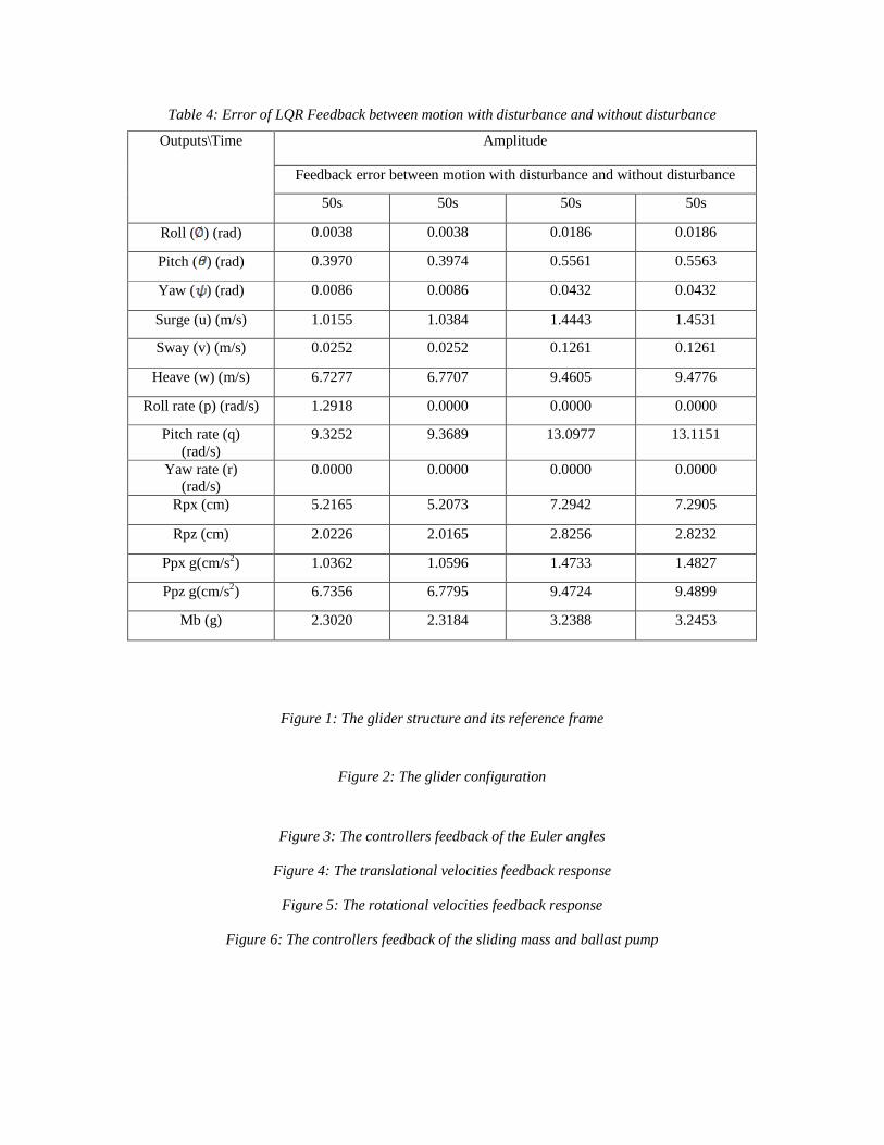
Table 4: Error of LQR Feedback between motion with disturbance and without disturbance

Amplitude

Feedback error between motion with disturbance and without disturbance

Outputs\Time

50s 50s 50s 50s

Roll ( ) (rad) 0.0038 0.0038 0.0186 0.0186

Pitch ( ) (rad) 0.3970 0.3974 0.5561 0.5563

Yaw ( ) (rad) 0.0086 0.0086 0.0432 0.0432

Surge (u) (m/s) 1.0155 1.0384 1.4443 1.4531

Sway (v) (m/s) 0.0252 0.0252 0.1261 0.1261

Heave (w) (m/s) 6.7277 6.7707 9.4605 9.4776

Roll rate (p) (rad/s) 1.2918 0.0000 0.0000 0.0000

Pitch rate (q)

(rad/s)

9.3252 9.3689 13.0977 13.1151

Yaw rate (r)

(rad/s)

0.0000 0.0000 0.0000 0.0000

Rpx (cm) 5.2165 5.2073 7.2942 7.2905

Rpz (cm) 2.0226 2.0165 2.8256 2.8232

Ppx g(cm/s2) 1.0362 1.0596 1.4733 1.4827

Ppz g(cm/s2) 6.7356 6.7795 9.4724 9.4899

Mb (g) 2.3020 2.3184 3.2388 3.2453

Figure 1: The glider structure and its reference frame

Figure 2: The glider configuration

Figure 3: The controllers feedback of the Euler angles

Figure 4: The translational velocities feedback response

Figure 5: The rotational velocities feedback response

Figure 6: The controllers feedback of the sliding mass and ballast pump