Robust Hybrid Control Systems

UNIVERSITY of CALIFORNIA

Santa Barbara

Robust Hybrid Control Systems

A Dissertation submitted in partial satisfaction of the

requirements for the degree

Doctor of Philosophy

in

Electrical and Computer Engineering

by

Ricardo G. Sanfelice

Committee in charge:

Professor Andrew R. Teel, Chair

Professor Petar V. Kokotovic

Professor Joao P. Hespanha

Professor Bassam Bamieh

September 2007


Copyright c© 20071

by


1Revised on January 2008.

To my mother Alicia, and my father Adolfo

iii

Acknowledgements

I am deeply grateful to my advisor, mentor, and friend Andy Teel for having guided me through the challengesof academic life and for teaching me to strive for elegance and mathematical rigor in my research. He hascontinuously motivated me to think creatively and to always aim for high-quality research.

I would like to express my gratitude to my family and friends who have given me constant emotional andspiritual support and encouragement throughout my doctorate program. In particular, I want to thank my wifeChristine who has been bold and remained supportive even in the busiest times of this journey.

I also want to thank the faculty in the Department of Electrical and Computer Engineering and in the Centerof Control, Dynamics, and Computation who directly or indirectly have shaped my career. In particular, I wantto thank Petar Kokotovic and Joao Hespanha for their encouragement, advice, and friendship throughout theyears. I thank all of the members of my doctoral committee for insightful discussions and useful suggestionsmade to improve this document.

I am grateful to my fellow graduate students, post-docs, and visitors who made graduate school an enjoyableexperience and were always available for discussions. I offer special thanks to Rafal Goebel for his helpfulcomments, advice and friendship; and to Gene, Doca, Ryan, Emre, Dragan, Michael, Max, James, Cai, Sara,Prabir, Payam, Kavyesh, Diane, Chris, and Josh who have been my lab-mates and friends.

Finally, I am thankful for the help I have received from the Center for Control, Dynamical Systems’ assistantsduring the last five years who have aided me very efficiently in the administrative paper work. I am also gratefulfor the financial support provided by the University of California Santa Barbara and the Office of InternationalStudents and Schoolars, and through my advisor by the National Science Foundation, Air Force Office ofScientific Research, and Army Research Office.

iv

Abstract


by


This thesis deals with systems exhibiting both continuous and discrete dynamics, perhaps due to intrinsicbehavior or to the interaction of continuous-time and discrete-time dynamics emerging from its componentsand/or their interconnection. Such systems are called hybrid systems and permit the modeling of a wide rangeof engineering systems and scientific processes. In this thesis, hybrid systems are treated as dynamical systems:the interplay between continuous and discrete behavior is captured in a mathematical model given by differentialequations/inclusions and difference equations/inclusions, which we simply call hybrid equations.

We develop tools for systematic analysis and robust design of hybrid systems, with an emphasis on systemsthat involve control algorithms, that is, hybrid control systems. To this effect, we identify mild conditions thathybrid equations need to satisfy so that their behavior captures the effect of arbitrarily small perturbations. Thisleads to novel concepts of generalized solutions that impart a deep understanding not only on the robustnessproperties of hybrid systems but also on the structural properties of their solutions. In turn, these conditionsenable us to generate various tools for hybrid systems that resemble those in the stability theory of classicaldynamical systems. These include general versions of Lyapunov and Krasovskii stability theorems, and LaSalle-type invariance principles. Additionally, we establish results on robustness of stability of hybrid control forgeneral nonlinear systems. We also present a novel mathematical framework for numerical simulation of hybridsystems and its asymptotic stability properties.

The contributions of this thesis are not limited to the theory of hybrid systems as they have implications inthe analysis and design of practically relevant engineering control systems. In this regard, we develop generalcontrol strategies for dynamical systems that are applicable, for example, to autonomous vehicles, multi-linkpendulums, and juggling systems.

v

Notation

• Rn denotes n-dimensional Euclidean space.

• R denotes the real numbers.

• Z denotes the integers.

• R≥0 denotes the nonnegative real numbers, i.e., R≥0 = [0,∞).

• N denotes the natural numbers including 0, i.e., N = 0, 1, . . ..

• B denotes the open unit ball in Euclidean space.

• Given a set S, S denotes its closure.

• Given a set S, coS denotes the convex hull and coS the closure of the convex hull.

• Given a set S ⊂ Rn and a point x ∈ R

n, |x|S := infy∈S |x− y|.

• Given sets S1, S2 ⊂ Rn, dH(S1, S2) denotes the Hausdorff distance between S1 and S2.

• Given sets S1, S2 subsets of Rn, S1 + S2 := x1 + x2 | x1 ∈ S1, x2 ∈ S2 .

• Given a vector x ∈ Rn, |x| denotes the Euclidean vector norm.

• The equivalent notation [xT yT ]T , [x y]T , and (x, y) is used for vectors.

• The notation f−1(r) stands for the r-level set of f on dom f , the domain of definition of f , i.e., f−1(r) :=z ∈ dom f | f(z) = r.

• A function α : R≥0 → R≥0 is said to belong to the class K if it is continuous, zero at zero, and strictlyincreasing.

• A function α : R≥0 → R≥0 is said to belong to the class K∞ if it belongs to the class K and is unbounded.

• A function β : R≥0 × R≥0 → R≥0 is said to belong to class-KL if it is continuous, nondecreasing in itsfirst argument, nonincreasing in its second argument, and limsց0 β(s, t) = limt→∞ β(s, t) = 0.

• A function β : R≥0 ×R≥0 ×R≥0 → R≥0 is said to belong to class-KLL if, for each r ∈ R≥0, the functionsβ(·, ·, r) and β(·, r, ·) belong to class-KL.

vi

Contents

Acknowledgments iv

Abstract v

Notation vi

List of Figures xi

1 Introduction 1

1.1 Dynamical modeling from a robustness viewpoint . . . . . . . . . . . . . . . . . . . . . . . . . . . 1

1.2 Tools for systematic analysis and design . . . . . . . . . . . . . . . . . . . . . . . . . . . . . . . . 3

1.3 Control strategies for robust stability . . . . . . . . . . . . . . . . . . . . . . . . . . . . . . . . . . 5

1.4 Robustness of numerical simulations . . . . . . . . . . . . . . . . . . . . . . . . . . . . . . . . . . 6

1.5 Notes . . . . . . . . . . . . . . . . . . . . . . . . . . . . . . . . . . . . . . . . . . . . . . . . . . . 7

2 Mathematical Model and Solutions 8

2.1 Preliminaries . . . . . . . . . . . . . . . . . . . . . . . . . . . . . . . . . . . . . . . . . . . . . . . 8

2.2 The model . . . . . . . . . . . . . . . . . . . . . . . . . . . . . . . . . . . . . . . . . . . . . . . . . 9

2.2.1 Examples . . . . . . . . . . . . . . . . . . . . . . . . . . . . . . . . . . . . . . . . . . . . . 10

2.2.2 Hysteresis in feedback control . . . . . . . . . . . . . . . . . . . . . . . . . . . . . . . . . . 13

2.3 Time domains and arcs . . . . . . . . . . . . . . . . . . . . . . . . . . . . . . . . . . . . . . . . . 16

2.4 Solutions to hybrid systems . . . . . . . . . . . . . . . . . . . . . . . . . . . . . . . . . . . . . . . 19

2.5 Examples and further modeling . . . . . . . . . . . . . . . . . . . . . . . . . . . . . . . . . . . . . 21

2.5.1 Bouncing ball revisited . . . . . . . . . . . . . . . . . . . . . . . . . . . . . . . . . . . . . . 21

2.5.2 Hybrid automaton . . . . . . . . . . . . . . . . . . . . . . . . . . . . . . . . . . . . . . . . 23

2.6 Summary . . . . . . . . . . . . . . . . . . . . . . . . . . . . . . . . . . . . . . . . . . . . . . . . . 23

2.7 Notes and references . . . . . . . . . . . . . . . . . . . . . . . . . . . . . . . . . . . . . . . . . . . 24

vii

3 Generalized Solutions 26

3.1 Hybrid systems with state perturbations . . . . . . . . . . . . . . . . . . . . . . . . . . . . . . . . 26

3.2 Generalized solutions to hybrid systems . . . . . . . . . . . . . . . . . . . . . . . . . . . . . . . . 30

3.3 Measurement noise in feedback control . . . . . . . . . . . . . . . . . . . . . . . . . . . . . . . . . 34

3.4 Regular hybrid systems . . . . . . . . . . . . . . . . . . . . . . . . . . . . . . . . . . . . . . . . . 38

3.5 Summary . . . . . . . . . . . . . . . . . . . . . . . . . . . . . . . . . . . . . . . . . . . . . . . . . 40


4 Stability and Invariance 42

4.1 Stability . . . . . . . . . . . . . . . . . . . . . . . . . . . . . . . . . . . . . . . . . . . . . . . . . . 42

4.1.1 Definitions . . . . . . . . . . . . . . . . . . . . . . . . . . . . . . . . . . . . . . . . . . . . 42

4.1.2 Lyapunov theorems . . . . . . . . . . . . . . . . . . . . . . . . . . . . . . . . . . . . . . . 43

4.2 Invariance . . . . . . . . . . . . . . . . . . . . . . . . . . . . . . . . . . . . . . . . . . . . . . . . . 45

4.2.1 Preliminaries . . . . . . . . . . . . . . . . . . . . . . . . . . . . . . . . . . . . . . . . . . . 45

4.2.2 Properties of Ω-limits sets . . . . . . . . . . . . . . . . . . . . . . . . . . . . . . . . . . . . 46

4.2.3 Convergence via invariance principles . . . . . . . . . . . . . . . . . . . . . . . . . . . . . 49

4.2.4 Connections to observability and detectability . . . . . . . . . . . . . . . . . . . . . . . . . 54

4.3 Examples . . . . . . . . . . . . . . . . . . . . . . . . . . . . . . . . . . . . . . . . . . . . . . . . . 56

4.4 Summary . . . . . . . . . . . . . . . . . . . . . . . . . . . . . . . . . . . . . . . . . . . . . . . . . 64


5 Robustness of Hybrid Control 68

5.1 Hybrid control of nonlinear systems . . . . . . . . . . . . . . . . . . . . . . . . . . . . . . . . . . 68

5.2 Robustness to perturbations . . . . . . . . . . . . . . . . . . . . . . . . . . . . . . . . . . . . . . . 71

5.2.1 Robustness via filtered measurements . . . . . . . . . . . . . . . . . . . . . . . . . . . . . 71

5.2.2 Robustness to sensor and actuator dynamics . . . . . . . . . . . . . . . . . . . . . . . . . 73

5.2.3 Robustness to sensor dynamics and smoothing . . . . . . . . . . . . . . . . . . . . . . . . 74

5.3 Robustness to digital implementation . . . . . . . . . . . . . . . . . . . . . . . . . . . . . . . . . . 76

5.3.1 Sample-and-hold model . . . . . . . . . . . . . . . . . . . . . . . . . . . . . . . . . . . . . 76

5.3.2 Closed-loop system analysis . . . . . . . . . . . . . . . . . . . . . . . . . . . . . . . . . . . 77

5.4 A benchmark problem: robust global swing-up of a pendulum on a cart . . . . . . . . . . . . . . 79

5.5 Summary . . . . . . . . . . . . . . . . . . . . . . . . . . . . . . . . . . . . . . . . . . . . . . . . . 82


6 Hybrid Control Applications 85

viii

6.1 Hysteresis-based control . . . . . . . . . . . . . . . . . . . . . . . . . . . . . . . . . . . . . . . . . 85

6.1.1 A robustness motivation to hybrid control . . . . . . . . . . . . . . . . . . . . . . . . . . . 85

6.1.2 A general robustness issue . . . . . . . . . . . . . . . . . . . . . . . . . . . . . . . . . . . . 87

6.1.3 Control design and analysis . . . . . . . . . . . . . . . . . . . . . . . . . . . . . . . . . . . 90

6.1.4 Two numerical examples . . . . . . . . . . . . . . . . . . . . . . . . . . . . . . . . . . . . . 94

6.2 Throw-and-catch control . . . . . . . . . . . . . . . . . . . . . . . . . . . . . . . . . . . . . . . . . 97

6.2.1 An intuitive control strategy . . . . . . . . . . . . . . . . . . . . . . . . . . . . . . . . . . 97

6.2.2 Control design and analysis . . . . . . . . . . . . . . . . . . . . . . . . . . . . . . . . . . . 98

6.2.3 Application: robust global pendubot swing-up control . . . . . . . . . . . . . . . . . . . . 104

6.3 Trajectory tracking control for a class of juggling systems . . . . . . . . . . . . . . . . . . . . . . 109

6.3.1 Introduction . . . . . . . . . . . . . . . . . . . . . . . . . . . . . . . . . . . . . . . . . . . 109

6.3.2 Trajectory tracking approach to juggling control . . . . . . . . . . . . . . . . . . . . . . . 110

6.3.3 Single-ball juggling . . . . . . . . . . . . . . . . . . . . . . . . . . . . . . . . . . . . . . . . 111

6.3.4 Multiple-balls juggling control . . . . . . . . . . . . . . . . . . . . . . . . . . . . . . . . . . 119

6.4 Summary . . . . . . . . . . . . . . . . . . . . . . . . . . . . . . . . . . . . . . . . . . . . . . . . . 123


7 Simulation Theory 125

7.1 Introduction . . . . . . . . . . . . . . . . . . . . . . . . . . . . . . . . . . . . . . . . . . . . . . . . 125

7.2 Simulation model . . . . . . . . . . . . . . . . . . . . . . . . . . . . . . . . . . . . . . . . . . . . . 126

7.3 From hybrid to discrete . . . . . . . . . . . . . . . . . . . . . . . . . . . . . . . . . . . . . . . . . 127

7.4 Closeness and continuity properties . . . . . . . . . . . . . . . . . . . . . . . . . . . . . . . . . . . 129

7.4.1 Numerical example . . . . . . . . . . . . . . . . . . . . . . . . . . . . . . . . . . . . . . . . 132

7.5 Summary . . . . . . . . . . . . . . . . . . . . . . . . . . . . . . . . . . . . . . . . . . . . . . . . . 134


8 Conclusion 135

8.1 Summary . . . . . . . . . . . . . . . . . . . . . . . . . . . . . . . . . . . . . . . . . . . . . . . . . 135

8.2 Future directions . . . . . . . . . . . . . . . . . . . . . . . . . . . . . . . . . . . . . . . . . . . . . 136

A Simulating Hybrid Systems in Matlab/Simulink 138

A.1 Simulink Model . . . . . . . . . . . . . . . . . . . . . . . . . . . . . . . . . . . . . . . . . . . . . . 138

A.2 Continuous dynamics . . . . . . . . . . . . . . . . . . . . . . . . . . . . . . . . . . . . . . . . . . . 140

A.3 Jump Logic . . . . . . . . . . . . . . . . . . . . . . . . . . . . . . . . . . . . . . . . . . . . . . . . 140

A.4 Update Logic . . . . . . . . . . . . . . . . . . . . . . . . . . . . . . . . . . . . . . . . . . . . . . . 142

ix

A.5 Stop Logic . . . . . . . . . . . . . . . . . . . . . . . . . . . . . . . . . . . . . . . . . . . . . . . . . 143

A.6 Examples . . . . . . . . . . . . . . . . . . . . . . . . . . . . . . . . . . . . . . . . . . . . . . . . . 143

A.7 Notes . . . . . . . . . . . . . . . . . . . . . . . . . . . . . . . . . . . . . . . . . . . . . . . . . . . 151

B Proofs 155

B.1 Proofs of results in Chapter 3 . . . . . . . . . . . . . . . . . . . . . . . . . . . . . . . . . . . . . . 155

B.1.1 Proof of Theorem 3.11 and Corollary 3.15 . . . . . . . . . . . . . . . . . . . . . . . . . . . 155


B.2.1 Proof of Theorem 4.3 . . . . . . . . . . . . . . . . . . . . . . . . . . . . . . . . . . . . . . 162


B.2.3 Proof of Corollary 4.15 . . . . . . . . . . . . . . . . . . . . . . . . . . . . . . . . . . . . . . 162





B.3.1 Proof of Theorem 5.12 . . . . . . . . . . . . . . . . . . . . . . . . . . . . . . . . . . . . . 165



B.4.2 Proof of Corollary 6.7 . . . . . . . . . . . . . . . . . . . . . . . . . . . . . . . . . . . . . . 175





Bibliography 182

x

List of Figures

1.1 Solutions in continuous, discrete, and hybrid time domains. . . . . . . . . . . . . . . . . . . . . . 3

1.2 Hybrid control of a nonlinear system under perturbations . . . . . . . . . . . . . . . . . . . . . . 6

2.1 Bouncing ball system . . . . . . . . . . . . . . . . . . . . . . . . . . . . . . . . . . . . . . . . . . . 11

2.2 Bouncing ball data. . . . . . . . . . . . . . . . . . . . . . . . . . . . . . . . . . . . . . . . . . . . . 12

2.3 Digital control of a continuous-time nonlinear system with sample and hold devices. . . . . . . . 12

2.4 Hysteresis behavior . . . . . . . . . . . . . . . . . . . . . . . . . . . . . . . . . . . . . . . . . . . . 14

2.5 General hysteresis. . . . . . . . . . . . . . . . . . . . . . . . . . . . . . . . . . . . . . . . . . . . . 14

2.6 Closed-loop system combining local and global controllers. . . . . . . . . . . . . . . . . . . . . . . 15

2.7 Hybrid controller data for combining local and global controllers. . . . . . . . . . . . . . . . . . . 16

2.8 Hybrid time domain. . . . . . . . . . . . . . . . . . . . . . . . . . . . . . . . . . . . . . . . . . . . 17

2.9 Hybrid arc. . . . . . . . . . . . . . . . . . . . . . . . . . . . . . . . . . . . . . . . . . . . . . . . . 18

2.10 Hybrid arc types . . . . . . . . . . . . . . . . . . . . . . . . . . . . . . . . . . . . . . . . . . . . . 19

2.11 A solution to a hybrid system H. . . . . . . . . . . . . . . . . . . . . . . . . . . . . . . . . . . . . 20

2.12 Bouncing ball solutions and domains. . . . . . . . . . . . . . . . . . . . . . . . . . . . . . . . . . . 22

2.13 A CADLAG solution x to H (Example 2.8) . . . . . . . . . . . . . . . . . . . . . . . . . . . . . . 25

3.1 Flow and jump set for the hybrid system (Example 3.3). . . . . . . . . . . . . . . . . . . . . . . . 28

3.2 The effect of state perturbations (Example 3.4). . . . . . . . . . . . . . . . . . . . . . . . . . . . . 28

3.3 Flow map and solutions (Example 3.5). . . . . . . . . . . . . . . . . . . . . . . . . . . . . . . . . 29

3.4 Jump map and solutions to Example 3.6. . . . . . . . . . . . . . . . . . . . . . . . . . . . . . . . 30

3.5 Two hybrid arcs (τ, ε)-close. . . . . . . . . . . . . . . . . . . . . . . . . . . . . . . . . . . . . . . 31

3.6 Solutions to zero-crossing detection system in Example 3.12. . . . . . . . . . . . . . . . . . . . . . 33

3.7 Robust feedback controller data (Example 3.13). . . . . . . . . . . . . . . . . . . . . . . . . . . . 35

3.8 Steering a vehicle to its target. . . . . . . . . . . . . . . . . . . . . . . . . . . . . . . . . . . . . . 38

3.9 Hybrid controller for steering a vehicle to its target with modified sets. . . . . . . . . . . . . . . . 39

xi

3.10 Convergence of solutions to the hybrid system (Example 3.20). . . . . . . . . . . . . . . . . . . . 40

4.1 Solutions (Example 4.19) . . . . . . . . . . . . . . . . . . . . . . . . . . . . . . . . . . . . . . . . 51

4.2 Bouncing ball, Newton’s cradle, and inverted pendulum on a cart. . . . . . . . . . . . . . . . . . 57

4.3 A solution to the bouncing ball system. . . . . . . . . . . . . . . . . . . . . . . . . . . . . . . . . 58

5.1 Closed-loop system with noise and filtered measurements. . . . . . . . . . . . . . . . . . . . . . . 71

5.2 Closed-loop system with sensor and actuator dynamics. . . . . . . . . . . . . . . . . . . . . . . . 73

5.3 Closed-loop system with sensor dynamics and control smoothing. . . . . . . . . . . . . . . . . . . 75

5.4 Sample-and-hold control of a nonlinear system. . . . . . . . . . . . . . . . . . . . . . . . . . . . 76

5.5 Pendulum on a cart. . . . . . . . . . . . . . . . . . . . . . . . . . . . . . . . . . . . . . . . . . . . 79

5.6 Solution to pendulum swing up with hybrid control including sensor and actuator dynamics:noise variance σ = 0.1. . . . . . . . . . . . . . . . . . . . . . . . . . . . . . . . . . . . . . . . . . . 80

5.7 Solution to pendulum swing up with hybrid control including sensor and actuator dynamics:noise variance σ = 1. . . . . . . . . . . . . . . . . . . . . . . . . . . . . . . . . . . . . . . . . . . . 81

5.8 Control law and discrete mode for pendulum swing up with hybrid control including sensor andactuator dynamics: large noise case. . . . . . . . . . . . . . . . . . . . . . . . . . . . . . . . . . . 82

5.9 Solution of pendulum swing up with sample-and-hold implementation of hybrid control: variabletimer constants. . . . . . . . . . . . . . . . . . . . . . . . . . . . . . . . . . . . . . . . . . . . . . . 83

5.10 Solution of pendulum swing up with sample-and-hold implementation of hybrid control: fixedsampling timer constant. . . . . . . . . . . . . . . . . . . . . . . . . . . . . . . . . . . . . . . . . . 83

6.1 Global steering of an autonomous vehicle to different locations. . . . . . . . . . . . . . . . . . . . 86

6.2 Global steering to a target with obstacle avoidance. . . . . . . . . . . . . . . . . . . . . . . . . . . 87

6.3 Sets for the problems in Section 6.1.1. . . . . . . . . . . . . . . . . . . . . . . . . . . . . . . . . . 89

6.4 Closed-loop system data for the regulation to disconnected set of points problem. . . . . . . . . . 94

6.5 Global stabilization of a robotic arm to two isolated destinations. . . . . . . . . . . . . . . . . . . 95

6.6 Global stabilization with obstacle avoidance. . . . . . . . . . . . . . . . . . . . . . . . . . . . . . 96

6.7 Throw-and-catch control. . . . . . . . . . . . . . . . . . . . . . . . . . . . . . . . . . . . . . . . . 98

6.8 Swing up of a multi-link pendulum on a cart. . . . . . . . . . . . . . . . . . . . . . . . . . . . . . 98

6.9 Control of autonomous vehicles with limited information. . . . . . . . . . . . . . . . . . . . . . . 99

6.10 General case of directed tree and j-th path. . . . . . . . . . . . . . . . . . . . . . . . . . . . . . . 100

6.11 Sets designed for the throw-and-catch strategy. . . . . . . . . . . . . . . . . . . . . . . . . . . . . 102

6.12 The pendubot system. . . . . . . . . . . . . . . . . . . . . . . . . . . . . . . . . . . . . . . . . . . 104

6.13 Equilibrium configurations of the pendubot. . . . . . . . . . . . . . . . . . . . . . . . . . . . . . . 105

6.14 Control strategy for robust global stabilization of the pendubot to the upright condition. . . . . . 107

6.15 Simulation of the pendubot system with throw-and-catch hybrid control strategy. . . . . . . . . . 108

xii

6.16 One-degree of freedom juggler. . . . . . . . . . . . . . . . . . . . . . . . . . . . . . . . . . . . . . 109

6.17 Ball height and reference trajectories on hybrid time domains. . . . . . . . . . . . . . . . . . . . . 110

6.18 Reference trajectory describing a periodic juggling pattern. . . . . . . . . . . . . . . . . . . . . . 111

6.19 Ball and juggler position trajectories. . . . . . . . . . . . . . . . . . . . . . . . . . . . . . . . . . . 112

6.20 Main control idea for trajectory tracking of juggling systems. . . . . . . . . . . . . . . . . . . . . 113

6.21 Sequence of events during ball-robot impact. . . . . . . . . . . . . . . . . . . . . . . . . . . . . . 114

6.22 Simulation (#1) of one-degree of freedom juggler: one ball case. . . . . . . . . . . . . . . . . . . . 118

6.23 Simulation (#2) of one-degree of freedom juggler: one ball case. . . . . . . . . . . . . . . . . . . . 119

6.24 One-degree of freedom juggler: multiple balls case. . . . . . . . . . . . . . . . . . . . . . . . . . . 120

6.25 Simulation of one-degree of freedom juggler: two balls case. . . . . . . . . . . . . . . . . . . . . . 122

6.26 Simulation of one-degree of freedom juggler: two balls case, virtual states. . . . . . . . . . . . . . 122

6.27 Simulation of one-degree of freedom juggler: three balls case. . . . . . . . . . . . . . . . . . . . . 123

7.1 Solution and simulation to the bouncing ball model. . . . . . . . . . . . . . . . . . . . . . . . . . 127

7.2 Closeness of simulations to solutions to the bouncing ball. . . . . . . . . . . . . . . . . . . . . . . 133

7.3 Closeness of simulations to solutions to the bouncing ball (detail). . . . . . . . . . . . . . . . . . 134

A.1 Matlab/Simulink implementation of a hybrid system. . . . . . . . . . . . . . . . . . . . . . . . . . 139

A.2 Integrator. . . . . . . . . . . . . . . . . . . . . . . . . . . . . . . . . . . . . . . . . . . . . . . . . . 140

A.3 Continuous dynamics. . . . . . . . . . . . . . . . . . . . . . . . . . . . . . . . . . . . . . . . . . . 141

A.4 Jump Logic. . . . . . . . . . . . . . . . . . . . . . . . . . . . . . . . . . . . . . . . . . . . . . . . . 142

A.5 Update Logic. . . . . . . . . . . . . . . . . . . . . . . . . . . . . . . . . . . . . . . . . . . . . . . . 143

A.6 Stop Logic. . . . . . . . . . . . . . . . . . . . . . . . . . . . . . . . . . . . . . . . . . . . . . . . . 144

A.7 Solution to the bouncing ball example: height. . . . . . . . . . . . . . . . . . . . . . . . . . . . . 145

A.8 Solution to the bouncing ball example: velocity. . . . . . . . . . . . . . . . . . . . . . . . . . . . . 146

A.9 Hybrid arc corresponding to a solution to the bouncing ball example: height. . . . . . . . . . . . 147

A.10 Solution to Example A.2 with forced jumps logic. . . . . . . . . . . . . . . . . . . . . . . . . . . . 148

A.11 Solution to Example A.2 with forced flows logic. . . . . . . . . . . . . . . . . . . . . . . . . . . . 149

A.12 Solution to Example A.2 with random logic for flowing/jumping. . . . . . . . . . . . . . . . . . . 150

A.13 Solution to Example A.2 with random logic for flowing/jumping. . . . . . . . . . . . . . . . . . . 151

A.14 Solution to Example A.2 with random logic for flowing/jumping. Zoomed version. . . . . . . . . 152

A.15 Solution to Example A.2 with forced jump logic and different O. . . . . . . . . . . . . . . . . . . 153

A.16 Solution to Example A.2 with forced flow logic. . . . . . . . . . . . . . . . . . . . . . . . . . . . . 154

xiii

Chapter 1

Introduction

Driven by recent technological advances, most engineering systems combine analog and digital devices, interactthrough networks, conduct tasks collaboratively, and operate in environments filled with uncertainties. Thisongoing trend has been one of the thrusts for research on modeling, stability analysis, control design, validation,verification, planning, and simulation of systems exhibiting both continuous and discrete behavior.

Because of their heterogeneous composition, the word hybrid is attached to these systems, where the presenceof two different behaviors, continuous and discrete, is the cause of heterogeneity. Hybrid systems consist of alarge class of systems that have been studied during the last few decades in several areas of engineering andscience, and as a consequence, they adopt different names. These include hybrid automata, embedded systems,and mixed-signal systems, among others. Hybrid systems are prevalent as they permit the modeling of a widerange of engineering systems and scientific processes, they are sometimes induced by system design, and at othertimes, they appear as modeling abstractions.

This thesis takes a dynamical systems approach to hybrid systems in the sense that its continuous behavioris associated with the dynamics of a continuous-time system while its discrete behavior is related to the dynamicsof a discrete-time system. The goal in treating hybrid systems as hybrid dynamical systems (which throughoutthis thesis will be referred to as simply hybrid systems) is to deeply understand their stability and robustnessproperties. The main purpose of this thesis is to provide tools for analysis, design, and simulation of hybridsystems where hybrid phenomena is not only intrinsic to the system but also induced by some external controlmechanism. This broad class of hybrid systems is referred to as hybrid control systems.

1.1 Dynamical modeling from a robustness viewpoint

Over the last few decades, in research areas such as computer science, feedback control, and dynamical systems,researchers have given considerable attention to modeling and solution definitions for hybrid systems. Perhapsthe earliest related reference is the work in [105] where a class of continuous-time systems with both continuousand discrete states (the state is referred to as hybrid state) exhibiting transitions was proposed in the contextof optimal control. More recent contributions model hybrid phenomena as differential, hybrid, and automata[97, 74, 43, 14, 103, 67, 98]; impulsive systems and inclusions [11, 7, 40]; continuous-time systems with discreteevents [4, 61]; among several others.

1

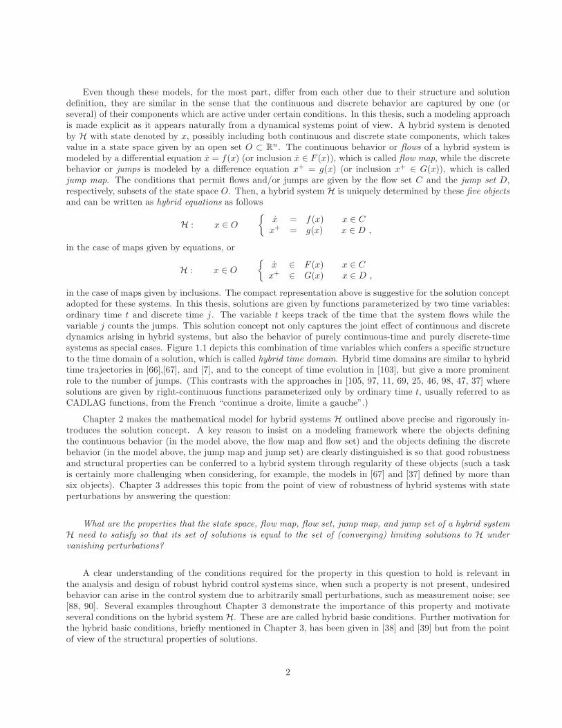
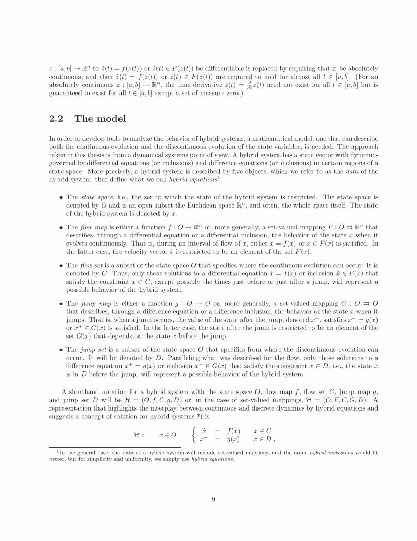
Even though these models, for the most part, differ from each other due to their structure and solutiondefinition, they are similar in the sense that the continuous and discrete behavior are captured by one (orseveral) of their components which are active under certain conditions. In this thesis, such a modeling approachis made explicit as it appears naturally from a dynamical systems point of view. A hybrid system is denotedby H with state denoted by x, possibly including both continuous and discrete state components, which takesvalue in a state space given by an open set O ⊂ R

n. The continuous behavior or flows of a hybrid system ismodeled by a differential equation x = f(x) (or inclusion x ∈ F (x)), which is called flow map, while the discretebehavior or jumps is modeled by a difference equation x+ = g(x) (or inclusion x+ ∈ G(x)), which is calledjump map. The conditions that permit flows and/or jumps are given by the flow set C and the jump set D,respectively, subsets of the state space O. Then, a hybrid system H is uniquely determined by these five objectsand can be written as hybrid equations as follows

H : x ∈ O

x = f(x) x ∈ Cx+ = g(x) x ∈ D ,

in the case of maps given by equations, or

H : x ∈ O

x ∈ F (x) x ∈ Cx+ ∈ G(x) x ∈ D ,

in the case of maps given by inclusions. The compact representation above is suggestive for the solution conceptadopted for these systems. In this thesis, solutions are given by functions parameterized by two time variables:ordinary time t and discrete time j. The variable t keeps track of the time that the system flows while thevariable j counts the jumps. This solution concept not only captures the joint effect of continuous and discretedynamics arising in hybrid systems, but also the behavior of purely continuous-time and purely discrete-timesystems as special cases. Figure 1.1 depicts this combination of time variables which confers a specific structureto the time domain of a solution, which is called hybrid time domain. Hybrid time domains are similar to hybridtime trajectories in [66],[67], and [7], and to the concept of time evolution in [103], but give a more prominentrole to the number of jumps. (This contrasts with the approaches in [105, 97, 11, 69, 25, 46, 98, 47, 37] wheresolutions are given by right-continuous functions parameterized only by ordinary time t, usually referred to asCADLAG functions, from the French “continue a droite, limite a gauche”.)

Chapter 2 makes the mathematical model for hybrid systems H outlined above precise and rigorously in-troduces the solution concept. A key reason to insist on a modeling framework where the objects definingthe continuous behavior (in the model above, the flow map and flow set) and the objects defining the discretebehavior (in the model above, the jump map and jump set) are clearly distinguished is so that good robustnessand structural properties can be conferred to a hybrid system through regularity of these objects (such a taskis certainly more challenging when considering, for example, the models in [67] and [37] defined by more thansix objects). Chapter 3 addresses this topic from the point of view of robustness of hybrid systems with stateperturbations by answering the question:

What are the properties that the state space, flow map, flow set, jump map, and jump set of a hybrid systemH need to satisfy so that its set of solutions is equal to the set of (converging) limiting solutions to H undervanishing perturbations?

A clear understanding of the conditions required for the property in this question to hold is relevant inthe analysis and design of robust hybrid control systems since, when such a property is not present, undesiredbehavior can arise in the control system due to arbitrarily small perturbations, such as measurement noise; see[88, 90]. Several examples throughout Chapter 3 demonstrate the importance of this property and motivateseveral conditions on the hybrid system H. These are are called hybrid basic conditions. Further motivation forthe hybrid basic conditions, briefly mentioned in Chapter 3, has been given in [38] and [39] but from the pointof view of the structural properties of solutions.

2

Figure 1.1. Continuous, discrete, and hybrid solutions parameterized by t, j, and both t and j, respectively.The latter corresponds to the solution concept for hybrid systems H. Its domain is a hybrid time domain.

1.2 Tools for systematic analysis and design

The analysis and design tools for hybrid systems in Chapter 4 come in the form of Lyapunov stability theorems,LaSalle-like invariance principles, and their connections with observability and detectability [87, 89]. Systematictools of this type are the foundation of the systems theory for purely continuous-time and discrete-time systems.Among similar tools available for hybrid systems before this thesis (for an overview of some other stability resultsfor hybrid systems, see [70] and [32]), the tools presented in Chapter 4 generalize their classical versions forcontinuous-time and discrete-time systems to the hybrid setting by defining an equivalent notion of stabilityand providing intuitive extensions of the sufficient conditions for asymptotic stability as outlined below.

The standard notion of stability of a point or set for continuous-time and discrete-time systems: if a solu-tion “starts close” then “it stays close” to the point or set, can be adopted as the notion of stability for hybridsystems H: given a hybrid system H, a compact set (or equilibrium point) A ⊂ O is stable if:

For every ε > 0 there exists δ > 0 such that each solution to H starting in a δ-neighborhood of A stays ina ε-neighborhood of A in its domain of definition.

Similarly, the notion of attractivity can also be extended: A is attractive if 1:

1Note that these notions do not assume that solutions exist for arbitrarily long t and/or j. To denote this property, the prefix“pre” is added to these concepts when precisely defined in Chapter 4.

3

There exists a neighborhood of A from which solutions stay in O and the ones that exist for arbitrarily longt and/or j converge to A as t+ j goes unbounded.

With these definitions, and under the hybrid basic conditions, given a Lyapunov function V , continuouslydifferentiable and positive definite with respect to A, the checkable conditions that it needs to satisfy for A tobe stable and attractive, i.e., (locally) asymptotically stable, are simply

〈∇V (x), f(x)〉 < 0 ∀x ∈ C \ A ,

V (g(x)) − V (x) < 0 ∀x ∈ D \ A, V (g(x)) − V (x) ≤ 0 ∀x ∈ D ,

for the case of single-valued flow and jump maps, and

maxξ∈F (x)

〈∇V (x), ξ〉 < 0 ∀x ∈ C \ A ,

maxξ∈G(x)

V (ξ) − V (x) < 0 ∀x ∈ D \ A, maxξ∈G(x)

V (ξ) − V (x) ≤ 0 ∀x ∈ D ,

for the case of set-valued flow and jump maps, where ∇V (x) is the gradient of V at x. Chapter 4 statesthis result for the case of locally Lipschitz V . It also presents special cases of it including a hybrid version ofKrasovskii’s stability theorem [54].

The second part of Chapter 4 includes general invariance principles for hybrid systems. These are applicableeven in the cases when solutions are nonunique, depend semicontinuously with respect to initial conditions, andhave multiple jumps at the same instant. These type of behaviors are common in robust hybrid control systemsand current invariance principle results in the literature do not apply. (These include the invariance principles in[67] where uniqueness of solutions and continuity with respect to initial conditions is required, and in [25] wheresolutions with multiple jumps at an instant are not allowed and further quasi-continuity properties includinguniqueness of solutions are imposed.)

The invariance principles in Chapter 4 include a result that parallels LaSalle’s invariance principle2, pre-sented in [59, 60] for differential and difference equations. The notion of invariance is accommodated appropri-ately to allow for nonuniqueness of solutions. It is called weak invariance and is defined as follows:

Given a hybrid system H, a set M ⊂ O is weakly invariant if it is both:

Weakly forward invariant: if for each point ξ ∈ M there exists at least one solution to H starting fromξ that exist for arbitrarily long t and/or j and is contained in the set M for all t and j in its domain of definition.

Weakly backward invariant: if for each point ξ′ ∈ M and every positive number N there exists a point ξfrom which there exists at least one solution to H starting from ξ that is equal to ξ′ for some t∗,j∗ in its domainof definition with the property that t∗ + j∗ ≥ N , and that remains in M up to t∗,j∗.

Limiting this discussion to the case of single-valued flow and jump maps for simplicity, for a hybrid systemH satisfying the hybrid basic conditions, a continuously differentiable function V : R

n → R, and a nonemptyset U ⊂ R

n such that

〈∇V (x), f(x)〉 ≤ 0 ∀x ∈ C ∩ UV (g(x)) − V (x) ≤ 0 ∀x ∈ D ∩ U ,

2Also known as Barbashin-Krasovskii-LaSalle’s invariance principle. Never intending to discredit any of the authors’ contribution,for simplicity, this invariance principle is referred throughout this thesis as “LaSalle’s invariance principle”.

4

every solution x to H that is bounded, exists for arbitrarily long t and/or j, and remains in U is such thatconverges to the largest weakly invariant set contained in

〈∇V (x), f(x)〉 = 0 ∪ (V (g(x)) − V (x) = 0 ∩ g(V (g(x)) − V (x) = 0))(1.1)

intersected with V −1(r) ∩ U for some constant r ∈ V (U).

Expression (1.1) characterizes the set of points in which to search for an invariant set. The invariance notion,which involves both (weak) forward and backward invariance, reduces this set compared to results where onlyforward invariance is required. Note that the result automatically recovers the continuous-time and discrete-time versions of LaSalle’s invariance principle, which are obtained by omitting the terms to the right or to theleft of the union symbol in (1.1), respectively. Even though the intersection in the term at its right does notimprove the result when specialized to purely discrete-time systems, it does improve the result for the hybridcase. This is illustrated in an example in Chapter 4.

1.3 Control strategies for robust stability

Over the last fifteen years, researchers have begun to recognize the extra capabilities of hybrid control systemscompared to classical continuous-time control systems. For example, it is now well-known that hysteresisswitching control can stabilize large classes of nonholonomic systems even though stabilization is impossibleusing time-invariant continuous state feedback, and robust stabilization is impossible using time-invariant locallybounded feedback. See, for example, [49, 76]. Also, sample-and-hold control (a special type of hybrid feedback)can be used to achieve stabilization that is robust to measurement noise and fast sensor/actuator dynamics,even if such robustness is impossible using purely continuous-time feedback. See, for example, [95], [28], [53].

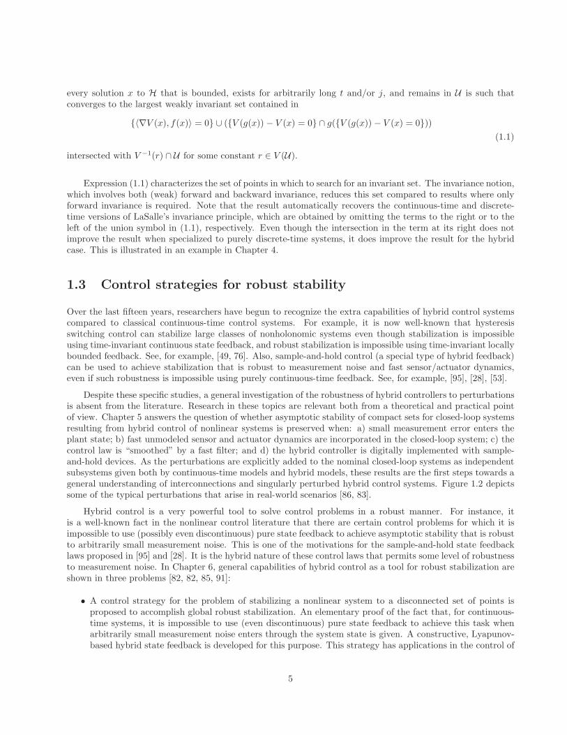
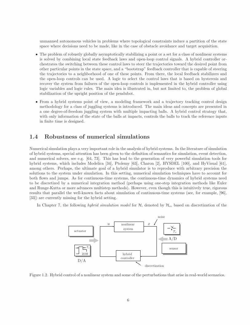
Despite these specific studies, a general investigation of the robustness of hybrid controllers to perturbationsis absent from the literature. Research in these topics are relevant both from a theoretical and practical pointof view. Chapter 5 answers the question of whether asymptotic stability of compact sets for closed-loop systemsresulting from hybrid control of nonlinear systems is preserved when: a) small measurement error enters theplant state; b) fast unmodeled sensor and actuator dynamics are incorporated in the closed-loop system; c) thecontrol law is “smoothed” by a fast filter; and d) the hybrid controller is digitally implemented with sample-and-hold devices. As the perturbations are explicitly added to the nominal closed-loop systems as independentsubsystems given both by continuous-time models and hybrid models, these results are the first steps towards ageneral understanding of interconnections and singularly perturbed hybrid control systems. Figure 1.2 depictssome of the typical perturbations that arise in real-world scenarios [86, 83].

Hybrid control is a very powerful tool to solve control problems in a robust manner. For instance, itis a well-known fact in the nonlinear control literature that there are certain control problems for which it isimpossible to use (possibly even discontinuous) pure state feedback to achieve asymptotic stability that is robustto arbitrarily small measurement noise. This is one of the motivations for the sample-and-hold state feedbacklaws proposed in [95] and [28]. It is the hybrid nature of these control laws that permits some level of robustnessto measurement noise. In Chapter 6, general capabilities of hybrid control as a tool for robust stabilization areshown in three problems [82, 82, 85, 91]:

• A control strategy for the problem of stabilizing a nonlinear system to a disconnected set of points isproposed to accomplish global robust stabilization. An elementary proof of the fact that, for continuous-time systems, it is impossible to use (even discontinuous) pure state feedback to achieve this task whenarbitrarily small measurement noise enters through the system state is given. A constructive, Lyapunov-based hybrid state feedback is developed for this purpose. This strategy has applications in the control of

5

unmanned autonomous vehicles in problems where topological constraints induce a partition of the statespace where decisions need to be made, like in the case of obstacle avoidance and target acquisition.

• The problem of robustly globally asymptotically stabilizing a point or a set for a class of nonlinear systemsis solved by combining local state feedback laws and open-loop control signals. A hybrid controller or-chestrates the switching between these control laws to steer the trajectories toward the desired point fromother particular points in the state space, and a “bootstrap” feedback controller that is capable of steeringthe trajectories to a neighborhood of one of these points. From there, the local feedback stabilizers andthe open-loop controls can be used. A logic to select the control laws that is based on hysteresis andrecover the system from failures of the open-loop controls is implemented in the hybrid controller usinglogic variables and logic rules. The main idea is illustrated in, but not limited to, the problem of globalstabilization of the upright position of the pendubot.

• From a hybrid systems point of view, a modeling framework and a trajectory tracking control designmethodology for a class of juggling systems is introduced. The main ideas and concepts are presented ina one degree-of-freedom juggling system with multiple impacting balls. A hybrid control strategy that,with only information of the state of the balls at impacts, controls the balls to track the reference inputsin finite time is designed.

1.4 Robustness of numerical simulations

Numerical simulation plays a very important role in the analysis of hybrid systems. In the literature of simulationof hybrid systems, special attention has been given to the definition of semantics for simulation, event detection,and numerical solvers, see e.g. [64, 73]. This has lead to the generation of very powerful simulation tools forhybrid systems, which includes Modelica [34], Ptolemy [63], Charon [2], HYSDEL [100], and HyVisual [61],among others. Perhaps, the ultimate goal of a hybrid simulator is to reproduce with arbitrary precision thesolutions to the system under simulation. In this setting, numerical simulation techniques have to account forboth flows and jumps. As for continuous-time systems, the continuous-time dynamics of hybrid systems needto be discretized by a numerical integration method (perhaps using one-step integration methods like Eulerand Runge-Kutta or more advances multistep methods). However, even though this is intuitively true, rigorousresults that parallel the well-known facts about simulation of continuous-time systems (see, for example, [96],[33]) are currently missing for the hybrid setting.

In Chapter 7, the following hybrid simulation model for H, denoted by Hs, based on discretization of the

Tc

Ts

xu

D/A

A/D

sensor

actuator

noise

discretization

controller

nonlinear

hybrid

system

ZOH

Figure 1.2. Hybrid control of a nonlinear system and some of the perturbations that arise in real-world scenarios.

6

dynamics is introduced:

Hs : x ∈ O

x+ ∈ Fs(x) x ∈ Cs

x+ ∈ Gs(x) x ∈ Ds

where s > 0 is the integration step, Fs is the integration scheme for the flows, Cs is a subset of Rn that indicates

where in the state space the integration scheme Fs works, Gs is the discrete mapping that simulates the jumps,and Ds is a subset of R

n that indicates where in the state space the mapping Gs for the simulation of jumpsworks. Note that the differential inclusion x ∈ F (x) was replaced by a difference inclusion. This corresponds tothe discretization of the flows. In Chapter 7, the following questions is addressed [84]:

What are the conditions on s, Fs, Cs, Gs, and Ds such that: 1) for a given simulation horizon, everysimulation to a hybrid system is arbitrarily close to an actual solution to the hybrid system; 2) asymptoticallystable compact sets for a hybrid system are semiglobally practically asymptotically stable compact sets for thehybrid simulator; 3) asymptotically stable compact sets for the hybrid simulator are continuous in the step size s?

The required properties are obtained by treating the hybrid simulator Hs as a perturbation of the hybridsystem H. The results make use of the recent results of asymptotic stability of compact sets for perturbedhybrid systems in [39].

1.5 Notes

The results outlined in the previous sections are given in the following chapters as indicated. More referencesand related material are included in the “Notes and references” section at the end of each of the followingchapters.

7

Chapter 2

Mathematical Model and Solutions

In this chapter, a mathematical model is introduced as a framework for modeling, analyzing, and designinghybrid systems. The description of the model is exercised by some of the examples exhibiting hybrid phenomenadiscussed in Chapter 1. The concept of solution in this framework is given by functions, called hybrid arcs, inextended time domains, called hybrid time domains. These concepts are illustrated through several examples.

2.1 Preliminaries

A set-valued mapping from Rm (or from a subset S of R

m) to Rn is understood to associate, with each point

x ∈ Rm (or x ∈ S), a subset of R

n. The notation M : Rm →→ R

n will distinguish a set-valued mapping M froma function.

Definition 2.1 (domain, range, graph)

Given a set-valued mapping M : Rm →→ R

n,

• the domain of M is the setdomM = x ∈ R

m | M(x) 6= ∅ ;

• the range of M is the set

rgeM = y ∈ Rn | ∃x ∈ R

m such that y ∈M(x) ;

• the graph of M is the setgphM = (x, y) ∈ R

m × Rn | y ∈M(x) .

A set-valued mapping M is fully determined by its graph, in the sense that

M(x) = y | (x, y) ∈ gphM .

A mapping M is empty-valued, single-valued, or multivalued at x if M(x) is empty, a singleton, or a setcontaining more than one element. Every function defined on a set S is a set-valued mapping that is single-valued at each point of S.

Solutions to differential equations and differential inclusions will be understood in the Caratheodory sense.That is, given a function f or a set-valued mapping F , the classical and very restrictive condition that a solution

8

z : [a, b] → Rn to z(t) = f(z(t)) or z(t) ∈ F (z(t)) be differentiable is replaced by requiring that it be absolutely

continuous, and then z(t) = f(z(t)) or z(t) ∈ F (z(t)) are required to hold for almost all t ∈ [a, b]. (For anabsolutely continuous z : [a, b] → R

n, the time derivative z(t) = ddtz(t) need not exist for all t ∈ [a, b] but is

guaranteed to exist for all t ∈ [a, b] except a set of measure zero.)

2.2 The model

In order to develop tools to analyze the behavior of hybrid systems, a mathematical model, one that can describeboth the continuous evolution and the discontinuous evolution of the state variables, is needed. The approachtaken in this thesis is from a dynamical systems point of view. A hybrid system has a state vector with dynamicsgoverned by differential equations (or inclusions) and difference equations (or inclusions) in certain regions of astate space. More precisely, a hybrid system is described by five objects, which we refer to as the data of thehybrid system, that define what we call hybrid equations1:

• The state space, i.e., the set to which the state of the hybrid system is restricted. The state space isdenoted by O and is an open subset the Euclidean space R

n, and often, the whole space itself. The stateof the hybrid system is denoted by x.

• The flow map is either a function f : O → Rn or, more generally, a set-valued mapping F : O →→ R

n thatdescribes, through a differential equation or a differential inclusion, the behavior of the state x when itevolves continuously. That is, during an interval of flow of x, either x = f(x) or x ∈ F (x) is satisfied. Inthe latter case, the velocity vector x is restricted to be an element of the set F (x).

• The flow set is a subset of the state space O that specifies where the continuous evolution can occur. It isdenoted by C. Thus, only those solutions to a differential equation x = f(x) or inclusion x ∈ F (x) thatsatisfy the constraint x ∈ C, except possibly the times just before or just after a jump, will represent apossible behavior of the hybrid system.

• The jump map is either a function g : O → O or, more generally, a set-valued mapping G : O →→ Othat describes, through a difference equation or a difference inclusion, the behavior of the state x when itjumps. That is, when a jump occurs, the value of the state after the jump, denoted x+, satisfies x+ = g(x)or x+ ∈ G(x) is satisfied. In the latter case, the state after the jump is restricted to be an element of theset G(x) that depends on the state x before the jump.

• The jump set is a subset of the state space O that specifies from where the discontinuous evolution canoccur. It will be denoted by D. Paralleling what was described for the flow, only those solutions to adifference equation x+ = g(x) or inclusion x+ ∈ G(x) that satisfy the constraint x ∈ D, i.e., the state xis in D before the jump, will represent a possible behavior of the hybrid system.

A shorthand notation for a hybrid system with the state space O, flow map f , flow set C, jump map g,and jump set D will be H = (O, f, C, g,D) or, in the case of set-valued mappings, H = (O,F,C,G,D). Arepresentation that highlights the interplay between continuous and discrete dynamics by hybrid equations andsuggests a concept of solution for hybrid systems H is

H : x ∈ O

x = f(x) x ∈ Cx+ = g(x) x ∈ D ,

1In the general case, the data of a hybrid system will include set-valued mappings and the name hybrid inclusions would fitbetter, but for simplicity and uniformity, we simply use hybrid equations.

9

respectively

H : x ∈ O

x ∈ F (x) x ∈ Cx+ ∈ G(x) x ∈ D .

(2.1)

The concept of solution will be rigorously stated in the next section, but the representation above suggests that

• solutions will stay in O;

• solutions will only be allowed to flow when in C and will satisfy x = f(x) (x ∈ F (x) in the set-valuedcase);

• solutions will only be allowed to jump when in D and the value after the jump will satisfy x+ = g(x) (orx+ ∈ G(x) in the set-valued case);

• at points where C and D overlap, solutions could be nonunique, that is, they could either flow or jump;

• from points in C where flows are not possible solutions will not be able to evolve forward;

• from points in O that are not in C ∪D, and from points where solutions that initially flow do it outsideof the set C, solutions will not exist.

An important property of the concept of solution used here that is worth it emphasizing is that solutions to Hcould be nonunique not only due to the flow and jump dynamics given by inclusions, but also because it couldbe that from certain points in the state space, solutions could both flow and jump.

Since functions can be viewed as a special (single-valued) case of set-valued mappings, from now on, unlessotherwise stated, set-valued mappings F and G as in (2.1) will be used in the symbolic description of hybridsystems. Note that this representation indicates that the proposed model for hybrid systems subsumes generalmodels for continuous-time and discrete-time systems when the jump map and jump set are empty, i.e., whendata is given by (O,F,C, ∅, ∅), and when the flow map and flow set are empty, i.e., when data is given by(O, ∅, ∅, G,D), respectively. This implies that the results in this thesis can be specialized, when appropriate, tothese dynamical system subclasses.

The hybrid phenomena discussed in Section 1 will be revisited with an emphasis on describing possiblechoices for the corresponding data that comprise the mathematical model as described above.

2.2.1 Examples

As illustrated in the following examples, hybrid phenomena, i.e. the typical behavior in hybrid systems, canarise naturally or can be induced by interconnections and logic.

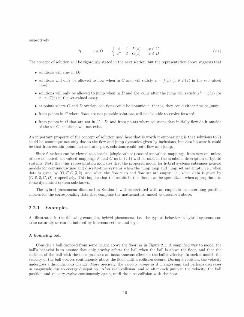
A bouncing ball

Consider a ball dropped from some height above the floor, as in Figure 2.1. A simplified way to model theball’s behavior is to assume that only gravity affects the ball when the ball is above the floor, and that thecollision of the ball with the floor produces an instantaneous effect on the ball’s velocity. In such a model, thevelocity of the ball evolves continuously above the floor until a collision occurs. During a collision, the velocityundergoes a discontinuous change. More precisely, the velocity jumps as it changes sign and perhaps decreasesin magnitude due to energy dissipation. After each collision, and so after each jump in the velocity, the ballposition and velocity evolve continuously again, until the next collision with the floor.

10

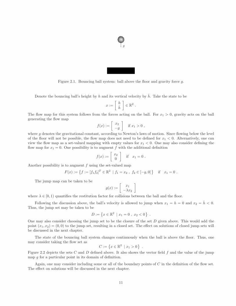
g

Figure 2.1. Bouncing ball system: ball above the floor and gravity force g.

Denote the bouncing ball’s height by h and its vertical velocity by h. Take the state to be

x :=

[h

h

]∈ R

2 .

The flow map for this system follows from the forces acting on the ball. For x1 > 0, gravity acts on the ballgenerating the flow map

f(x) :=

[x2

−g

]if x1 > 0 ,

where g denotes the gravitational constant, according to Newton’s laws of motion. Since flowing below the levelof the floor will not be possible, the flow map does not need to be defined for x1 < 0. Alternatively, one canview the flow map as a set-valued mapping with empty values for x1 < 0. One may also consider defining theflow map for x1 = 0. One possibility is to augment f with the additional definition

f(x) :=

[x2

0

]if x1 = 0 .

Another possibility is to augment f using the set-valued map

F (x) :=f := [f1f2]

T ∈ R2 | f1 = x2 , f2 ∈ [−g, 0]

if x1 = 0 .

The jump map can be taken to be

g(x) :=

[x1

−λx2

]

where λ ∈ [0, 1) quantifies the restitution factor for collisions between the ball and the floor.

Following the discussion above, the ball’s velocity is allowed to jump when x1 = h = 0 and x2 = h < 0.Thus, the jump set may be taken to be

D :=x ∈ R

2 | x1 = 0 , x2 < 0.

One may also consider choosing the jump set to be the closure of the set D given above. This would add thepoint (x1, x2) = (0, 0) to the jump set, resulting in a closed set. The effect on solutions of closed jump sets willbe discussed in the next chapter.

The state of the bouncing ball system changes continuously when the ball is above the floor. Thus, onemay consider taking the flow set as

C :=x ∈ R

2 | x1 > 0.

Figure 2.2 depicts the sets C and D defined above. It also shows the vector field f and the value of the jumpmap g for a particular point in its domain of definition.

Again, one may consider including some or all of the boundary points of C in the definition of the flow set.The effect on solutions will be discussed in the next chapter.

11

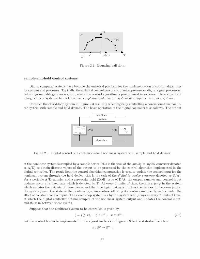
x1

x2x∗D

C

g(x∗)

f(x′)

Figure 2.2. Bouncing ball data.

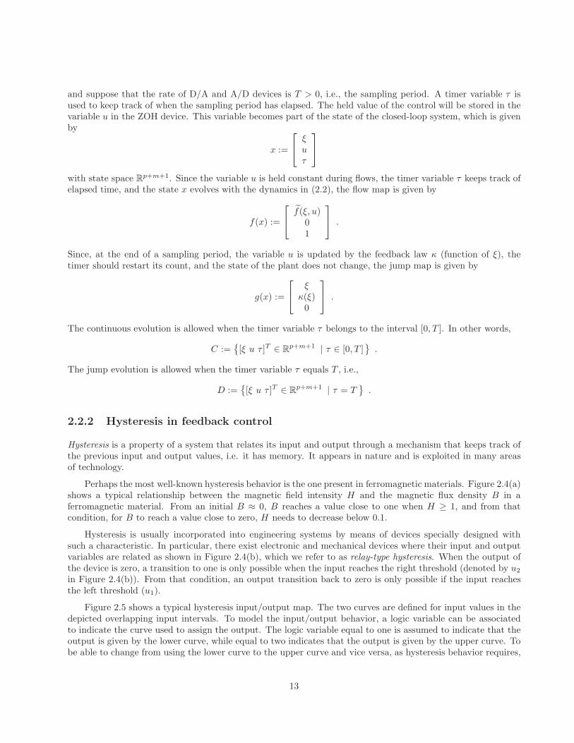
Sample-and-hold control systems

Digital computer systems have become the universal platform for the implementation of control algorithmsfor systems and processes. Typically, these digital controllers consist of microprocessors, digital signal processors,field-programmable gate arrays, etc., where the control algorithm is programmed in software. These constitutea large class of systems that is known as sample-and-hold control systems or computer controlled systems.

Consider the closed-loop system in Figure 2.3 resulting when digitally controlling a continuous-time nonlin-ear system with sample and hold devices. The basic operation of the digital controller is as follows. The output

ZOH

A/DD/AT

T

nonlinear

system

algorithm

Figure 2.3. Digital control of a continuous-time nonlinear system with sample and hold devices.

of the nonlinear system is sampled by a sample device (this is the task of the analog-to-digital converter denotedas A/D) to obtain discrete values of the output to be processed by the control algorithm implemented in thedigital controller. The result from the control algorithm computation is used to update the control input for thenonlinear system through the hold device (this is the task of the digital-to-analog converter denoted as D/A).For a periodic A/D sampler and a zero-order hold (ZOH) type of D/A, the output samples and control inputupdates occur at a fixed rate which is denoted by T . At every T units of time, there is a jump in the systemwhich updates the outputs of these blocks and the time logic that synchronizes the devices. In between jumps,the system flows: the state of the nonlinear system evolves following its continuous-time dynamics under theeffect of constant control input. The closed-loop system is a hybrid system with jumps at every T units of time,at which the digital controller obtains samples of the nonlinear system output and updates the control input,and flows in between those events.

Suppose that the nonlinear system to be controlled is given by

ξ = f(ξ, u), ξ ∈ Rp , u ∈ R

m . (2.2)

Let the control law to be implemented in the algorithm block in Figure 2.3 be the state-feedback law

κ : Rp → R

m ,

12

and suppose that the rate of D/A and A/D devices is T > 0, i.e., the sampling period. A timer variable τ isused to keep track of when the sampling period has elapsed. The held value of the control will be stored in thevariable u in the ZOH device. This variable becomes part of the state of the closed-loop system, which is givenby

x :=

ξuτ

with state space Rp+m+1. Since the variable u is held constant during flows, the timer variable τ keeps track of

elapsed time, and the state x evolves with the dynamics in (2.2), the flow map is given by

f(x) :=

f(ξ, u)

01

.

Since, at the end of a sampling period, the variable u is updated by the feedback law κ (function of ξ), thetimer should restart its count, and the state of the plant does not change, the jump map is given by

g(x) :=

ξ

κ(ξ)0

.

The continuous evolution is allowed when the timer variable τ belongs to the interval [0, T ]. In other words,

C :=[ξ u τ ]T ∈ R

p+m+1 | τ ∈ [0, T ].

The jump evolution is allowed when the timer variable τ equals T , i.e.,

D :=[ξ u τ ]T ∈ R

p+m+1 | τ = T.

2.2.2 Hysteresis in feedback control

Hysteresis is a property of a system that relates its input and output through a mechanism that keeps track ofthe previous input and output values, i.e. it has memory. It appears in nature and is exploited in many areasof technology.

Perhaps the most well-known hysteresis behavior is the one present in ferromagnetic materials. Figure 2.4(a)shows a typical relationship between the magnetic field intensity H and the magnetic flux density B in aferromagnetic material. From an initial B ≈ 0, B reaches a value close to one when H ≥ 1, and from thatcondition, for B to reach a value close to zero, H needs to decrease below 0.1.

Hysteresis is usually incorporated into engineering systems by means of devices specially designed withsuch a characteristic. In particular, there exist electronic and mechanical devices where their input and outputvariables are related as shown in Figure 2.4(b), which we refer to as relay-type hysteresis. When the output ofthe device is zero, a transition to one is only possible when the input reaches the right threshold (denoted by u2

in Figure 2.4(b)). From that condition, an output transition back to zero is only possible if the input reachesthe left threshold (u1).

Figure 2.5 shows a typical hysteresis input/output map. The two curves are defined for input values in thedepicted overlapping input intervals. To model the input/output behavior, a logic variable can be associatedto indicate the curve used to assign the output. The logic variable equal to one is assumed to indicate that theoutput is given by the lower curve, while equal to two indicates that the output is given by the upper curve. Tobe able to change from using the lower curve to the upper curve and vice versa, as hysteresis behavior requires,

13

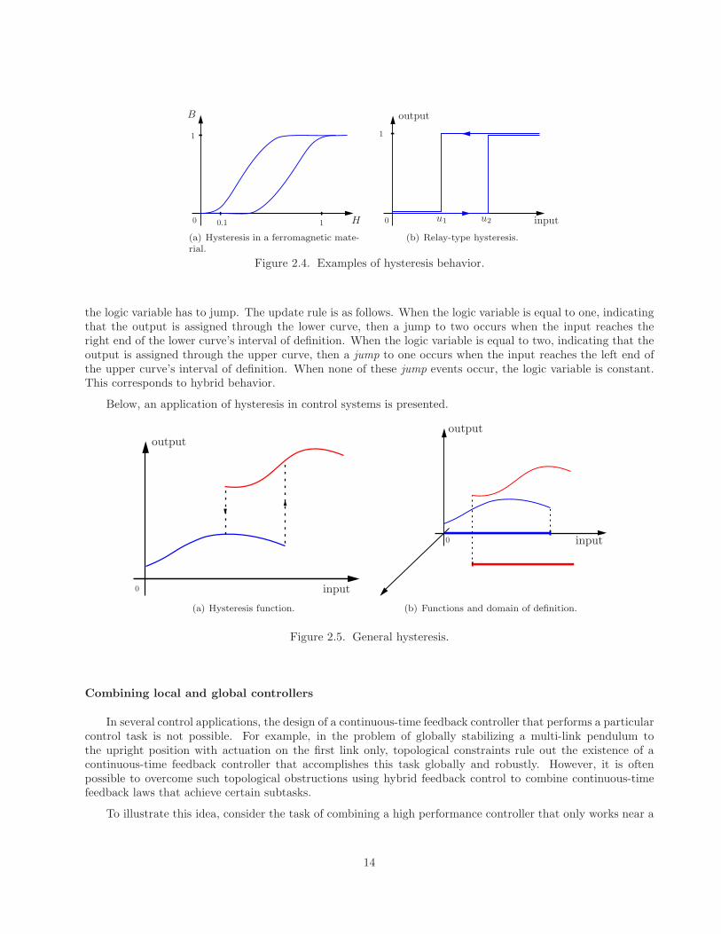
B

H1

1

0.10

(a) Hysteresis in a ferromagnetic mate-rial.

u1 u2 input

output

1

0

(b) Relay-type hysteresis.

Figure 2.4. Examples of hysteresis behavior.

the logic variable has to jump. The update rule is as follows. When the logic variable is equal to one, indicatingthat the output is assigned through the lower curve, then a jump to two occurs when the input reaches theright end of the lower curve’s interval of definition. When the logic variable is equal to two, indicating that theoutput is assigned through the upper curve, then a jump to one occurs when the input reaches the left end ofthe upper curve’s interval of definition. When none of these jump events occur, the logic variable is constant.This corresponds to hybrid behavior.

Below, an application of hysteresis in control systems is presented.

output

input0

(a) Hysteresis function.

output

input0

(b) Functions and domain of definition.

Figure 2.5. General hysteresis.

Combining local and global controllers

In several control applications, the design of a continuous-time feedback controller that performs a particularcontrol task is not possible. For example, in the problem of globally stabilizing a multi-link pendulum tothe upright position with actuation on the first link only, topological constraints rule out the existence of acontinuous-time feedback controller that accomplishes this task globally and robustly. However, it is oftenpossible to overcome such topological obstructions using hybrid feedback control to combine continuous-timefeedback laws that achieve certain subtasks.

To illustrate this idea, consider the task of combining a high performance controller that only works near a

14

prescribed operating point with a controller that is able to steer every trajectory to the operating point but doesnot have as good a performance near that point. We refer to these as local and global controllers, respectively.

reference

supervisor

local

global

controller

controller

eplant

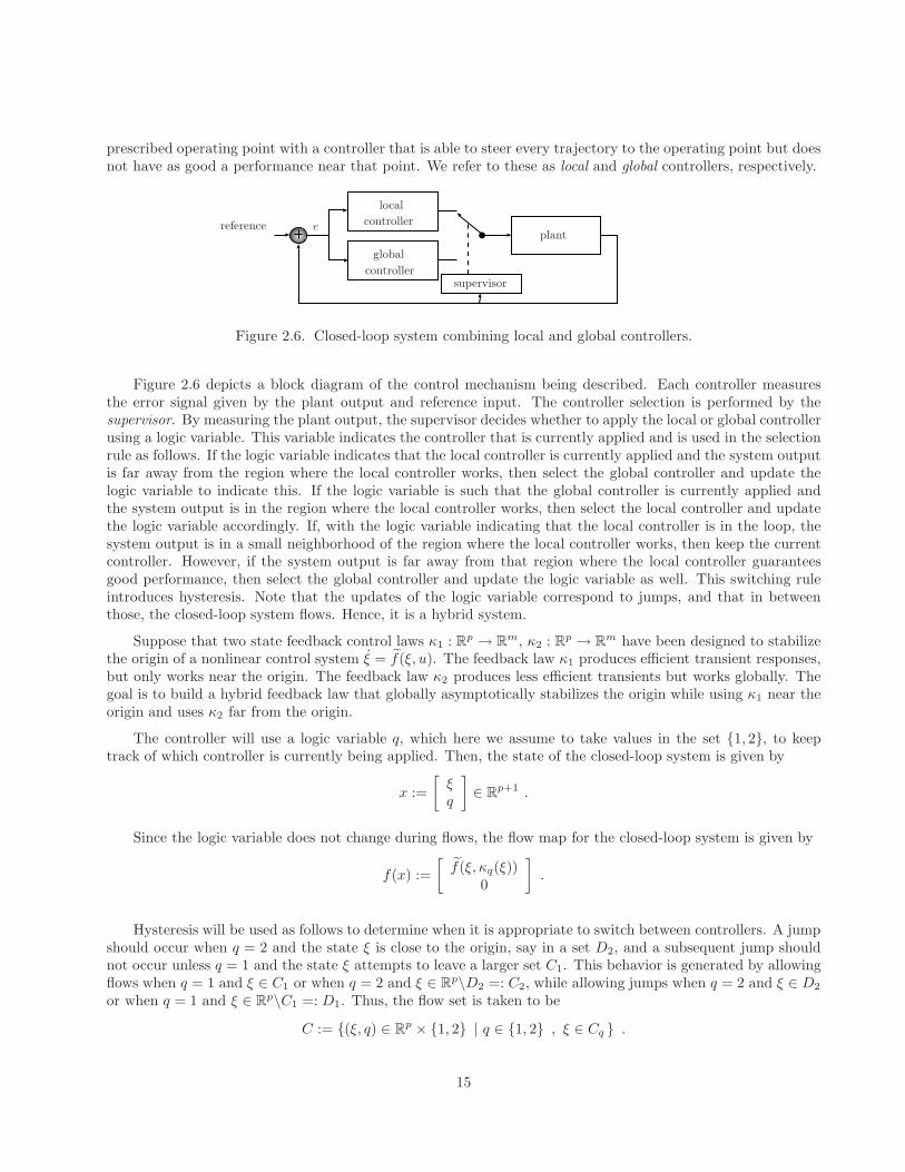
Figure 2.6. Closed-loop system combining local and global controllers.

Figure 2.6 depicts a block diagram of the control mechanism being described. Each controller measuresthe error signal given by the plant output and reference input. The controller selection is performed by thesupervisor. By measuring the plant output, the supervisor decides whether to apply the local or global controllerusing a logic variable. This variable indicates the controller that is currently applied and is used in the selectionrule as follows. If the logic variable indicates that the local controller is currently applied and the system outputis far away from the region where the local controller works, then select the global controller and update thelogic variable to indicate this. If the logic variable is such that the global controller is currently applied andthe system output is in the region where the local controller works, then select the local controller and updatethe logic variable accordingly. If, with the logic variable indicating that the local controller is in the loop, thesystem output is in a small neighborhood of the region where the local controller works, then keep the currentcontroller. However, if the system output is far away from that region where the local controller guaranteesgood performance, then select the global controller and update the logic variable as well. This switching ruleintroduces hysteresis. Note that the updates of the logic variable correspond to jumps, and that in betweenthose, the closed-loop system flows. Hence, it is a hybrid system.

Suppose that two state feedback control laws κ1 : Rp → R

m, κ2 : Rp → R

m have been designed to stabilizethe origin of a nonlinear control system ξ = f(ξ, u). The feedback law κ1 produces efficient transient responses,but only works near the origin. The feedback law κ2 produces less efficient transients but works globally. Thegoal is to build a hybrid feedback law that globally asymptotically stabilizes the origin while using κ1 near theorigin and uses κ2 far from the origin.

The controller will use a logic variable q, which here we assume to take values in the set 1, 2, to keeptrack of which controller is currently being applied. Then, the state of the closed-loop system is given by

x :=

[ξq

]∈ R

p+1 .

Since the logic variable does not change during flows, the flow map for the closed-loop system is given by

f(x) :=

[f(ξ, κq(ξ))

0

].

Hysteresis will be used as follows to determine when it is appropriate to switch between controllers. A jumpshould occur when q = 2 and the state ξ is close to the origin, say in a set D2, and a subsequent jump shouldnot occur unless q = 1 and the state ξ attempts to leave a larger set C1. This behavior is generated by allowingflows when q = 1 and ξ ∈ C1 or when q = 2 and ξ ∈ R

p\D2 =: C2, while allowing jumps when q = 2 and ξ ∈ D2

or when q = 1 and ξ ∈ Rp\C1 =: D1. Thus, the flow set is taken to be

C := (ξ, q) ∈ Rp × 1, 2 | q ∈ 1, 2 , ξ ∈ Cq .

15

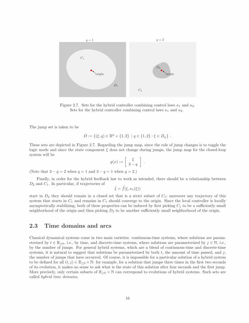
D1

D2

C1

C2

q = 1 q = 2

originorigin

Figure 2.7. Sets for the hybrid controller combining control laws κ1 and κ2.Sets for the hybrid controller combining control laws κ1 and κ2.

The jump set is taken to be

D := (ξ, q) ∈ Rp × 1, 2 | q ∈ 1, 2 : ξ ∈ Dq .

These sets are depicted in Figure 2.7. Regarding the jump map, since the role of jump changes is to toggle thelogic mode and since the state component ξ does not change during jumps, the jump map for the closed-loopsystem will be

g(x) :=

[ξ

3 − q

].

(Note that 3 − q = 2 when q = 1 and 3 − q = 1 when q = 2.)

Finally, in order for the hybrid feedback law to work as intended, there should be a relationship betweenD2 and C1. In particular, if trajectories of

ξ = f(ξ, κ1(ξ))

start in D2 they should remain in a closed set that is a strict subset of C1; moreover any trajectory of thissystem that starts in C1 and remains in C1 should converge to the origin. Since the local controller is locallyasymptotically stabilizing, both of these properties can be induced by first picking C1 to be a sufficiently smallneighborhood of the origin and then picking D2 to be another sufficiently small neighborhood of the origin.

2.3 Time domains and arcs

Classical dynamical systems come in two main varieties: continuous-time systems, where solutions are param-eterized by t ∈ R≥0, i.e., by time, and discrete-time systems, where solutions are parameterized by j ∈ N, i.e.,by the number of jumps. For general hybrid systems, which are a blend of continuous-time and discrete-timesystems, it is natural to suggest that solutions be parameterized by both t, the amount of time passed, and j,the number of jumps that have occurred. Of course, it is impossible for a particular solution of a hybrid systemto be defined for all (t, j) ∈ R≥0 ×N: for example, for a solution that jumps three times in the first two secondsof its evolution, it makes no sense to ask what is the state of this solution after four seconds and the first jump.More precisely, only certain subsets of R≥0 × N can correspond to evolutions of hybrid systems. Such sets arecalled hybrid time domains.

16

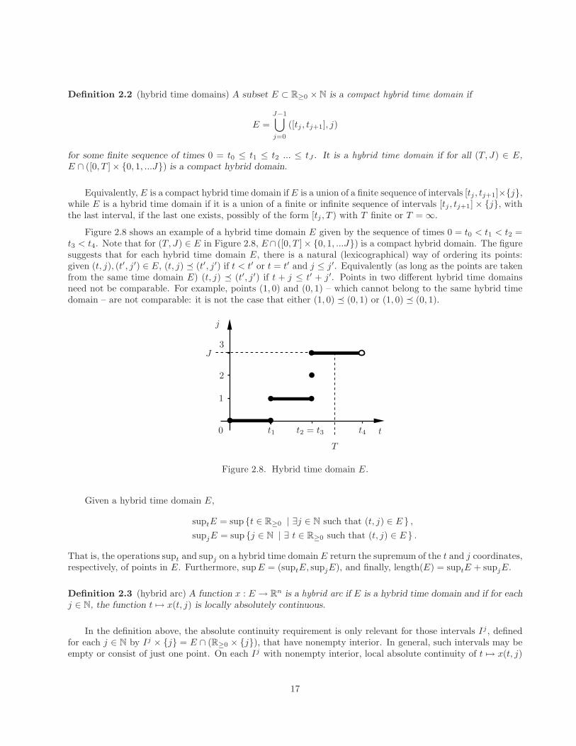
Definition 2.2 (hybrid time domains) A subset E ⊂ R≥0 × N is a compact hybrid time domain if

E =J−1⋃

j=0

([tj , tj+1], j)

for some finite sequence of times 0 = t0 ≤ t1 ≤ t2 ... ≤ tJ . It is a hybrid time domain if for all (T, J) ∈ E,E ∩ ([0, T ]× 0, 1, ...J) is a compact hybrid domain.

Equivalently, E is a compact hybrid time domain if E is a union of a finite sequence of intervals [tj , tj+1]×j,while E is a hybrid time domain if it is a union of a finite or infinite sequence of intervals [tj , tj+1] × j, withthe last interval, if the last one exists, possibly of the form [tj , T ) with T finite or T = ∞.

Figure 2.8 shows an example of a hybrid time domain E given by the sequence of times 0 = t0 < t1 < t2 =t3 < t4. Note that for (T, J) ∈ E in Figure 2.8, E∩ ([0, T ]× 0, 1, ...J) is a compact hybrid domain. The figuresuggests that for each hybrid time domain E, there is a natural (lexicographical) way of ordering its points:given (t, j), (t′, j′) ∈ E, (t, j) (t′, j′) if t < t′ or t = t′ and j ≤ j′. Equivalently (as long as the points are takenfrom the same time domain E) (t, j) (t′, j′) if t + j ≤ t′ + j′. Points in two different hybrid time domainsneed not be comparable. For example, points (1, 0) and (0, 1) – which cannot belong to the same hybrid timedomain – are not comparable: it is not the case that either (1, 0) (0, 1) or (1, 0) (0, 1).

0

1

2

3

t1 t2 = t3 t4 t

j

T

J

Figure 2.8. Hybrid time domain E.

Given a hybrid time domain E,

suptE = sup t ∈ R≥0 | ∃j ∈ N such that (t, j) ∈ E ,supjE = sup j ∈ N | ∃ t ∈ R≥0 such that (t, j) ∈ E .

That is, the operations supt and supj on a hybrid time domain E return the supremum of the t and j coordinates,respectively, of points in E. Furthermore, supE = (suptE, supjE), and finally, length(E) = suptE + supjE.

Definition 2.3 (hybrid arc) A function x : E → Rn is a hybrid arc if E is a hybrid time domain and if for each

j ∈ N, the function t 7→ x(t, j) is locally absolutely continuous.

In the definition above, the absolute continuity requirement is only relevant for those intervals Ij , definedfor each j ∈ N by Ij × j = E ∩ (R≥0 × j), that have nonempty interior. In general, such intervals may beempty or consist of just one point. On each Ij with nonempty interior, local absolute continuity of t 7→ x(t, j)

17

means that t 7→ x(t, j) is absolutely continuous on each compact subinterval of Ij . Also, on each such Ij ,t 7→ x(t, j) is differentiable almost everywhere, and x(t, j) will denote the time derivative of x(t, j), whenever itexists. In short,

x(t, j) =d

dtx(t, j).

Given a hybrid arc x, the notation domx represents its domain, which is a hybrid time domain. Suchnotation is consistent with the following “set-valued interpretation” of a hybrid arc. A hybrid arc x can bedefined as a set-valued mapping x : R

2 →→ Rn that is single-valued on its domain domx (i.e., on the set of (t, j)

on which x(t, j) 6= ∅, recall Definition 2.1) which is a hybrid time domain and for which t 7→ x(t, j) is locallyabsolutely continuous for each fixed j ∈ N. Such interpretation makes it more natural to think that the hybridtime domain domx is determined by the arc x. This will be particularly relevant when talking about hybridarcs that are solutions to a hybrid system. Then, it is certainly not appropriate to consider (an arbitrary)hybrid time domain E first, and then try to find a solution with E as a domain. Rather, it is necessary to find asolution x first, and say that its domain domx is determined by x. Furthermore, the “set-valued interpretation”above will help carry over some concepts of convergence and closeness of mappings from the set-valued realmto hybrid arcs and to solutions of hybrid systems, in later chapters.

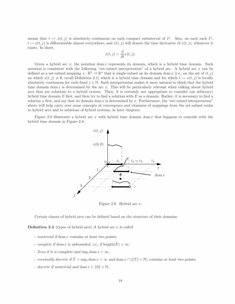
Figure 2.9 illustrates a hybrid arc x with hybrid time domain domx that happens to coincide with thehybrid time domain in Figure 2.8.

0

1

2

3

t1 t2 = t3 t4

j

t

x(0, 0)

x(t, j)

domx

Figure 2.9. Hybrid arc x.

Certain classes of hybrid arcs can be defined based on the structure of their domains.

Definition 2.4 (types of hybrid arcs) A hybrid arc x is called

- nontrivial if domx contains at least two points;

- complete if domx is unbounded, i.e., if length(E) = ∞;

- Zeno if it is complete and supt domx <∞;

- eventually discrete if T = supt domx <∞ and domx ∩ (T × N) contains at least two points;

- discrete if nontrivial and domx ⊂ 0 × N;

18

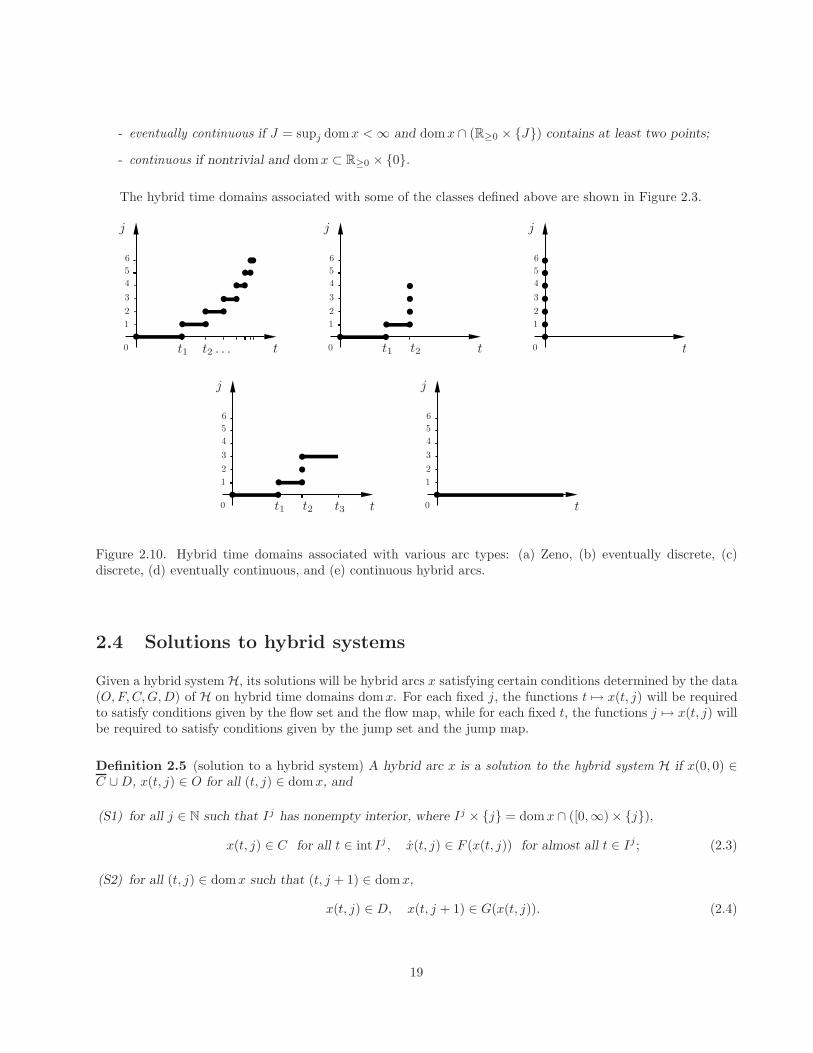
- eventually continuous if J = supj domx <∞ and domx ∩ (R≥0 × J) contains at least two points;

- continuous if nontrivial and domx ⊂ R≥0 × 0.

The hybrid time domains associated with some of the classes defined above are shown in Figure 2.3.

0

1

2

3

4

5

6

t1 t2 . . . t

j

0

1

2

3

4

5

6

t1 t2 t

j

0

1

2

3

4

5

6

t

j

0

1

2

3

4

5

6

t1 t2 t3 t

j

0

1

2

3

4

5

6

t

j

Figure 2.10. Hybrid time domains associated with various arc types: (a) Zeno, (b) eventually discrete, (c)discrete, (d) eventually continuous, and (e) continuous hybrid arcs.

2.4 Solutions to hybrid systems

Given a hybrid system H, its solutions will be hybrid arcs x satisfying certain conditions determined by the data(O,F,C,G,D) of H on hybrid time domains domx. For each fixed j, the functions t 7→ x(t, j) will be requiredto satisfy conditions given by the flow set and the flow map, while for each fixed t, the functions j 7→ x(t, j) willbe required to satisfy conditions given by the jump set and the jump map.

Definition 2.5 (solution to a hybrid system) A hybrid arc x is a solution to the hybrid system H if x(0, 0) ∈C ∪D, x(t, j) ∈ O for all (t, j) ∈ domx, and

(S1) for all j ∈ N such that Ij has nonempty interior, where Ij × j = domx ∩ ([0,∞) × j),

x(t, j) ∈ C for all t ∈ int Ij , x(t, j) ∈ F (x(t, j)) for almost all t ∈ Ij ; (2.3)

(S2) for all (t, j) ∈ domx such that (t, j + 1) ∈ domx,

x(t, j) ∈ D, x(t, j + 1) ∈ G(x(t, j)). (2.4)

19

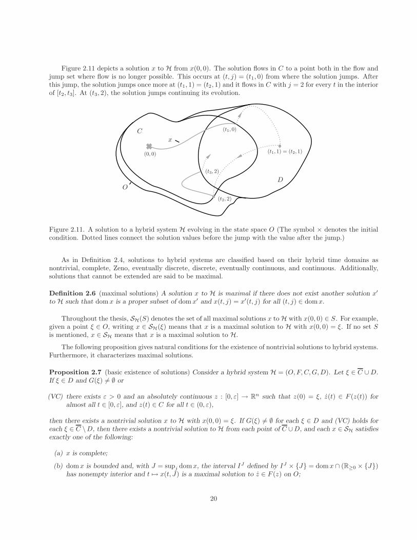
Figure 2.11 depicts a solution x to H from x(0, 0). The solution flows in C to a point both in the flow andjump set where flow is no longer possible. This occurs at (t, j) = (t1, 0) from where the solution jumps. Afterthis jump, the solution jumps once more at (t1, 1) = (t2, 1) and it flows in C with j = 2 for every t in the interiorof [t2, t3]. At (t3, 2), the solution jumps continuing its evolution.

(0, 0)

(t1, 0)

(t1, 1) = (t2, 1)

(t2, 2)

(t3, 2)

xC

DO

Figure 2.11. A solution to a hybrid system H evolving in the state space O (The symbol × denotes the initialcondition. Dotted lines connect the solution values before the jump with the value after the jump.)

As in Definition 2.4, solutions to hybrid systems are classified based on their hybrid time domains asnontrivial, complete, Zeno, eventually discrete, discrete, eventually continuous, and continuous. Additionally,solutions that cannot be extended are said to be maximal.

Definition 2.6 (maximal solutions) A solution x to H is maximal if there does not exist another solution x′

to H such that domx is a proper subset of domx′ and x(t, j) = x′(t, j) for all (t, j) ∈ domx.

Throughout the thesis, SH(S) denotes the set of all maximal solutions x to H with x(0, 0) ∈ S. For example,given a point ξ ∈ O, writing x ∈ SH(ξ) means that x is a maximal solution to H with x(0, 0) = ξ. If no set Sis mentioned, x ∈ SH means that x is a maximal solution to H.

The following proposition gives natural conditions for the existence of nontrivial solutions to hybrid systems.Furthermore, it characterizes maximal solutions.

Proposition 2.7 (basic existence of solutions) Consider a hybrid system H = (O,F,C,G,D). Let ξ ∈ C ∪D.If ξ ∈ D and G(ξ) 6= ∅ or

(VC) there exists ε > 0 and an absolutely continuous z : [0, ε] → Rn such that z(0) = ξ, z(t) ∈ F (z(t)) for

almost all t ∈ [0, ε], and z(t) ∈ C for all t ∈ (0, ε),

then there exists a nontrivial solution x to H with x(0, 0) = ξ. If G(ξ) 6= ∅ for each ξ ∈ D and (VC) holds foreach ξ ∈ C \D, then there exists a nontrivial solution to H from each point of C ∪D, and each x ∈ SH satisfiesexactly one of the following:

(a) x is complete;

(b) domx is bounded and, with J = supj domx, the interval IJ defined by IJ × J = domx ∩ (R≥0 × J)has nonempty interior and t 7→ x(t, J) is a maximal solution to z ∈ F (z) on O;

20

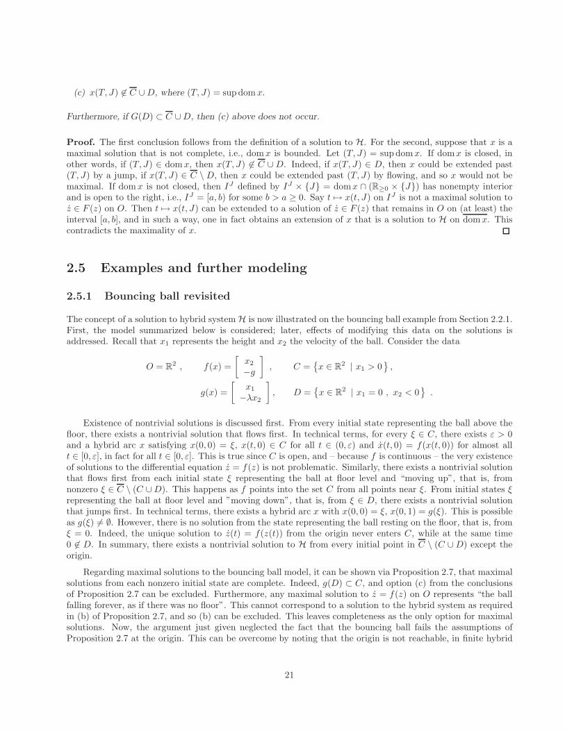
(c) x(T, J) 6∈ C ∪D, where (T, J) = sup domx.

Furthermore, if G(D) ⊂ C ∪D, then (c) above does not occur.

Proof. The first conclusion follows from the definition of a solution to H. For the second, suppose that x is amaximal solution that is not complete, i.e., domx is bounded. Let (T, J) = sup domx. If domx is closed, inother words, if (T, J) ∈ domx, then x(T, J) 6∈ C ∪ D. Indeed, if x(T, J) ∈ D, then x could be extended past(T, J) by a jump, if x(T, J) ∈ C \D, then x could be extended past (T, J) by flowing, and so x would not bemaximal. If domx is not closed, then IJ defined by IJ × J = domx ∩ (R≥0 × J) has nonempty interiorand is open to the right, i.e., IJ = [a, b) for some b > a ≥ 0. Say t 7→ x(t, J) on IJ is not a maximal solution toz ∈ F (z) on O. Then t 7→ x(t, J) can be extended to a solution of z ∈ F (z) that remains in O on (at least) theinterval [a, b], and in such a way, one in fact obtains an extension of x that is a solution to H on domx. Thiscontradicts the maximality of x.

2.5 Examples and further modeling

2.5.1 Bouncing ball revisited

The concept of a solution to hybrid system H is now illustrated on the bouncing ball example from Section 2.2.1.First, the model summarized below is considered; later, effects of modifying this data on the solutions isaddressed. Recall that x1 represents the height and x2 the velocity of the ball. Consider the data

O = R2 , f(x) =

[x2

−g

], C =

x ∈ R

2 | x1 > 0,

g(x) =

[x1

−λx2

], D =

x ∈ R

2 | x1 = 0 , x2 < 0.

Existence of nontrivial solutions is discussed first. From every initial state representing the ball above thefloor, there exists a nontrivial solution that flows first. In technical terms, for every ξ ∈ C, there exists ε > 0and a hybrid arc x satisfying x(0, 0) = ξ, x(t, 0) ∈ C for all t ∈ (0, ε) and x(t, 0) = f(x(t, 0)) for almost allt ∈ [0, ε], in fact for all t ∈ [0, ε]. This is true since C is open, and – because f is continuous – the very existenceof solutions to the differential equation z = f(z) is not problematic. Similarly, there exists a nontrivial solutionthat flows first from each initial state ξ representing the ball at floor level and “moving up”, that is, fromnonzero ξ ∈ C \ (C ∪D). This happens as f points into the set C from all points near ξ. From initial states ξrepresenting the ball at floor level and ”moving down”, that is, from ξ ∈ D, there exists a nontrivial solutionthat jumps first. In technical terms, there exists a hybrid arc x with x(0, 0) = ξ, x(0, 1) = g(ξ). This is possibleas g(ξ) 6= ∅. However, there is no solution from the state representing the ball resting on the floor, that is, fromξ = 0. Indeed, the unique solution to z(t) = f(z(t)) from the origin never enters C, while at the same time0 6∈ D. In summary, there exists a nontrivial solution to H from every initial point in C \ (C ∪D) except theorigin.

Regarding maximal solutions to the bouncing ball model, it can be shown via Proposition 2.7, that maximalsolutions from each nonzero initial state are complete. Indeed, g(D) ⊂ C, and option (c) from the conclusionsof Proposition 2.7 can be excluded. Furthermore, any maximal solution to z = f(z) on O represents “the ballfalling forever, as if there was no floor”. This cannot correspond to a solution to the hybrid system as requiredin (b) of Proposition 2.7, and so (b) can be excluded. This leaves completeness as the only option for maximalsolutions. Now, the argument just given neglected the fact that the bouncing ball fails the assumptions ofProposition 2.7 at the origin. This can be overcome by noting that the origin is not reachable, in finite hybrid

21

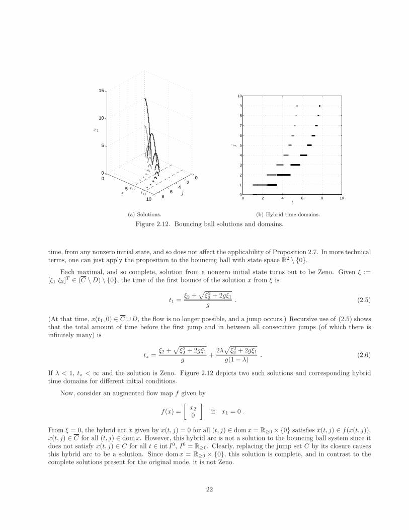
02

46

8

0

5

10

0

5

10

15

jt

x1

tz1

tz2

(a) Solutions.

0 2 4 6 8 100

1

2

3

4

5

6

7

8

9

10

j

t

(b) Hybrid time domains.

Figure 2.12. Bouncing ball solutions and domains.

time, from any nonzero initial state, and so does not affect the applicability of Proposition 2.7. In more technicalterms, one can just apply the proposition to the bouncing ball with state space R

2 \ 0.Each maximal, and so complete, solution from a nonzero initial state turns out to be Zeno. Given ξ :=

[ξ1 ξ2]T ∈ (C \D) \ 0, the time of the first bounce of the solution x from ξ is

t1 =ξ2 +

√ξ22 + 2gξ1g

. (2.5)

(At that time, x(t1, 0) ∈ C ∪D, the flow is no longer possible, and a jump occurs.) Recursive use of (2.5) showsthat the total amount of time before the first jump and in between all consecutive jumps (of which there isinfinitely many) is

tz =ξ2 +

√ξ22 + 2gξ1g

+2λ

√ξ22 + 2gξ1

g(1 − λ). (2.6)

If λ < 1, tz < ∞ and the solution is Zeno. Figure 2.12 depicts two such solutions and corresponding hybridtime domains for different initial conditions.

Now, consider an augmented flow map f given by

f(x) =

[x2

0

]if x1 = 0 .

From ξ = 0, the hybrid arc x given by x(t, j) = 0 for all (t, j) ∈ domx = R≥0 × 0 satisfies x(t, j) ∈ f(x(t, j)),x(t, j) ∈ C for all (t, j) ∈ domx. However, this hybrid arc is not a solution to the bouncing ball system since itdoes not satisfy x(t, j) ∈ C for all t ∈ int I0, I0 = R≥0. Clearly, replacing the jump set C by its closure causesthis hybrid arc to be a solution. Since domx = R≥0 × 0, this solution is complete, and in contrast to thecomplete solutions present for the original mode, it is not Zeno.

22

Existence of a solution from the origin can be guaranteed if, instead, the point ξ = 0 is added to the jumpset D. With this modification, a constant complete and discrete solution from ξ exists. Indeed, g(D)∩D = 0and x(0, j) = 0 for all j ∈ N with domx = 0 × N is a solution. While allowing such a hybrid arc to be asolution of the bouncing ball model may seem counter intuitive, it can – and will be in later chapters – motivatedby the pursuit of robustness of hybrid system models. Indeed, this solution reflects the nature of solutions frominitial points in C ∪D arbitrarily close to 0 – all such solutions are Zeno.

2.5.2 Hybrid automaton

With appropriate choice of data, hybrid systems H can model systems where the “discrete variable” q is explicitlymentioned. More specifically, consider

H :

z = fq(z) z ∈ Cq[z+

q+

]∈ Gq(z) z ∈ Dq ,

(2.7)

where Q is the set of “modes”, and for each q ∈ Q, fq : Cq → Rm, Cq ⊂ R

m, Gq : Dq →→ Rm ×Q, and Dq ⊂ R

m.When Q can be identified with a subset of integers (and so a subset of R), we can consider a system in the form(2.1) with the variable x = [z q]T ∈ R

m+1 and data

f(x) =

[fq(z)

0

], C =

⋃

q∈Q

(Cq × q), G(x) = Gq(z), D =⋃

q∈Q

(Dq × q) . (2.8)

In turn, systems in the form (2.7) easily capture the commonly encountered hybrid automata where data isgiven in terms of domains, guards, edges, and resets, Let Q be the set of “modes”, for each q ∈ Q let fq be theflow map, let the mapping Domain : Q→→ R

m give the domains of flow, let Edges ⊂ Q×Q be the set of edges,Guard : Edges →→ R

m be the mapping giving the guards, and Reset : Edges×Rm →→ R

m be the reset map. Onethen takes

Cq = Domain(q), Dq =⋃

e=(q,q′)∈Edges

Guard(e), (2.9)

Gq(x) =⋃

e = (q, q′) s.t.x ∈ Guard(e)

[Reset(e, x)

q′

]. (2.10)

Note that a set-valued mapping Gq will arise this way when two guard sets, Guard(e′) with e′ = (q, q′) andGuard(e′′) with e′′ = (q, q′′), overlap. This will even be the case when the resets Reset(e′, ·) and Reset(e′′, ·) aresingle valued. Solutions to the hybrid automaton by hybrid arcs are such that, for a fixed value of the discretestate q, the continuous state evolves with dynamics given by z = fq(z), and once the jump set D is reached(given by Dq which corresponds to the current Guard), jumps are possible with the rule determined by the resetmap Reset.

2.6 Summary

A modeling framework for hybrid systems has been introduced. Hybrid systems are given by hybrid equationswith a state space O, a flow map given by a single-valued function f or a set-valued mapping F , a flow setC ⊂ O, a jump map given by a single-valued function g or a set-valued mapping G, and a jump set D. The

23

shorthand notation for a hybrid system is H = (O, f, C, g,D) or H = (O,F,C,G,D) in the set-valued case.Solutions are given by hybrid arcs and parameterized by (t, j) on hybrid time domains, which are subsets ofR≥0 × N. Depending on the hybrid time domain, solutions (or more generally, hybrid arcs) can be nontrivial,complete, Zeno, eventually discrete, discrete, eventually continuous, and continuous. Moreover, solutions thatcannot be extended are called maximal. Several examples illustrated this modeling framework.

2.7 Notes and references

In what could be described as a “classical” approach to dynamical systems with jumps, the candidates for asolution are considered to be piecewise continuous functions of time that are right continuous and have leftlimits at each t in their domain of definition. This approach has been used in the early work by Witsenhausen[105] and Tavernini [97], and more recently in [11, 69, 25, 46, 98, 47, 37]. (Functions that are right continuousand have left limits are frequently referred to in the literature as CADLAG, from the French “continue a droite,limite a gauche”.)

More precisely, a CADLAG solution to H = (O, f, C, g,D) is a function ξ : [0, T ] → Rn or ξ : [0, T ) → R

n

that is piecewise absolutely continuous (or piecewise differentiable), has a finite number of discontinuities in eachcompact subset of the interval on which it is defined, and that at every t it has left limits, is right continuous,and:

(D1) on each interval of continuityξ(t) ∈ C, ξ(t) = f(ξ(t));

(D2) at all points τ > 0 of discontinuity satisfies

ξ−(τ) ∈ D, ξ(τ) ∈ g(ξ−(τ));

where ξ−(τ) := limtրτ ξ(t). Whether ξ(t) = f(ξ(t)) is to be understood as true for all t or for almost all t dependson whether one considers ξ’s that are differentiable on the intervals of continuity, or just absolutely continuous.By design, such a concept of a solution excludes multiple jumps at a single time instant. Furthermore, it makesit troublesome (or impossible) to discuss limits of solutions as the following example shows.

Example 2.8 (rotate and dissipate) Consider a hybrid system H on R2 given by

x = f(x) :=

[x2

−x1

]x ∈ C := R

2,

x+ = g(x) :=x

2x ∈ D := (0, 1) × 0 .

For any point ξ with 0 < |ξ| < 1 and ξ 6∈ D, a CADLAG solution from ξ exists. One such solution rotatesclockwise around the origin for all time. (Such a solution will be excluded if D is considered to “force” jumpsrather than “enable” them.) Another solution rotates clockwise until it hitsD, then via a jump has its magnitudedivided by 2, and then rotates again for 2π units of time until it hits D again at which point in time it jumps,and this cycle repeats for all time. Figure 2.13 depicts a solution of this type up to the second jump. Othersolutions are created by rotating clockwise around the origin when not in D and permitting a jump wheneverin D.

There are additional solutions that are admitted when using hybrid time domains that are not admittedwhen using CADLAG functions. In particular, the hybrid arc that corresponds to rotating clockwise aroundthe origin until hitting D and then making an infinite number of jumps, each one cutting the magnitude of thesolution in half, is a solution since each jump maps a point in D to another point in D.

24

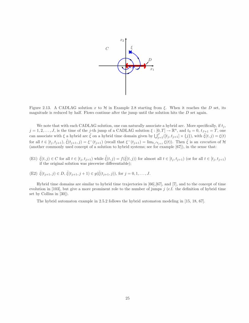
C

D

ξ

x1

x2

Figure 2.13. A CADLAG solution x to H in Example 2.8 starting from ξ. When it reaches the D set, itsmagnitude is reduced by half. Flows continue after the jump until the solution hits the D set again.

We note that with each CADLAG solution, one can naturally associate a hybrid arc. More specifically, if tj ,j = 1, 2, . . . , J , is the time of the j-th jump of a CADLAG solution ξ : [0, T ] → R

n, and t0 = 0, tJ+1 = T , one

can associate with ξ a hybrid arc ξ on a hybrid time domain given by⋃J

j=1([tj , tj+1] × j), with ξ(t, j) = ξ(t)

for all t ∈ [tj , tj+1), ξ(tj+1, j) = ξ−(tj+1) (recall that ξ−(tj+1) = limtրtj+1 ξ(t)). Then ξ is an execution of H(another commonly used concept of a solution to hybrid systems; see for example [67]), in the sense that:

(E1) ξ(t, j) ∈ C for all t ∈ [tj , tj+1) while˙ξ(t, j) = f(ξ(t, j)) for almost all t ∈ [tj , tj+1) (or for all t ∈ [tj , tj+1)

if the original solution was piecewise differentiable);

(E2) ξ(tj+1, j) ∈ D, ξ(tj+1, j + 1) ∈ g(ξ(tj+1, j)), for j = 0, 1, . . . , J .

Hybrid time domains are similar to hybrid time trajectories in [66],[67], and [7], and to the concept of timeevolution in [103], but give a more prominent role to the number of jumps j (c.f. the definition of hybrid timeset by Collins in [30]).

The hybrid automaton example in 2.5.2 follows the hybrid automaton modeling in [15, 18, 67].

25

Chapter 3

Generalized Solutions

This chapter discusses the effect of state perturbations on the solutions to a hybrid system. It is shownthat state perturbations, of arbitrarily small size, can dramatically change the behavior of solutions. Thisbehavior is related to the properties of the data of a hybrid system. A regularization procedure that resultsin a hybrid system with a set of “generalized solutions” that captures all limiting solutions with measurementnoise converging to zero is proposed. This leads to and motivates the regularity conditions on the data ofhybrid systems, called hybrid basic conditions, that will be required when deriving the results in the subsequentchapters.

3.1 Hybrid systems with state perturbations

A hybrid system H = (O,F,C,G,D) with a state perturbation e is denoted by He, and following (2.1), will bewritten in the suggestive form:

He : x+ e ∈ O

x ∈ F (x+ e) x+ e ∈ Cx+ ∈ G(x+ e) x+ e ∈ D .

(3.1)

Before formally defining solutions to He, a class of admissible state perturbation is specified.

Definition 3.1 (admissible state perturbation) A mapping e is an admissible state perturbation if dom e is ahybrid time domain and the function t→ e(t, j) is measurable on dom e ∩ (R≥0 × j) for each j ∈ N.

In several instances, the naturally arising state perturbation entering a hybrid system is dependent ontime t ∈ R≥0 only, and not on j. For example, this is the case when a nonlinear control system is controlledby switching between several state-feedback laws, and the switching – which is what makes the closed-loopsystem hybrid – is not affected by the state perturbation. In such cases, any measurable signal e′ : R≥0 → R

n

corresponding to the state perturbation can be considered as given on an arbitrary hybrid time domain E, bysetting

e(t, j) := e′(t) (t, j) ∈ dom e := E . (3.2)

A formal definition of solutions to He with admissible state perturbation e follows.

26

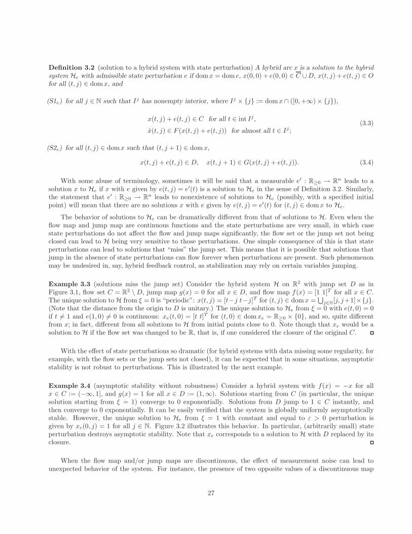
Definition 3.2 (solution to a hybrid system with state perturbation) A hybrid arc x is a solution to the hybridsystem He with admissible state perturbation e if domx = dom e, x(0, 0) + e(0, 0) ∈ C ∪D, x(t, j) + e(t, j) ∈ Ofor all (t, j) ∈ domx, and

(S1e) for all j ∈ N such that Ij has nonempty interior, where Ij × j := domx ∩ ([0,+∞)× j),

x(t, j) + e(t, j) ∈ C for all t ∈ int Ij ,

x(t, j) ∈ F (x(t, j) + e(t, j)) for almost all t ∈ Ij ;(3.3)

(S2e) for all (t, j) ∈ domx such that (t, j + 1) ∈ domx,

x(t, j) + e(t, j) ∈ D, x(t, j + 1) ∈ G(x(t, j) + e(t, j)). (3.4)

With some abuse of terminology, sometimes it will be said that a measurable e′ : R≥0 → Rn leads to a

solution x to He if x with e given by e(t, j) = e′(t) is a solution to He in the sense of Definition 3.2. Similarly,the statement that e′ : R≥0 → R

n leads to nonexistence of solutions to He (possibly, with a specified initialpoint) will mean that there are no solutions x with e given by e(t, j) = e′(t) for (t, j) ∈ domx to He.

The behavior of solutions to He can be dramatically different from that of solutions to H. Even when theflow map and jump map are continuous functions and the state perturbations are very small, in which casestate perturbations do not affect the flow and jump maps significantly, the flow set or the jump set not beingclosed can lead to H being very sensitive to those perturbations. One simple consequence of this is that stateperturbations can lead to solutions that “miss” the jump set. This means that it is possible that solutions thatjump in the absence of state perturbations can flow forever when perturbations are present. Such phenomenonmay be undesired in, say, hybrid feedback control, as stabilization may rely on certain variables jumping.

Example 3.3 (solutions miss the jump set) Consider the hybrid system H on R2 with jump set D as in

Figure 3.1, flow set C = R2 \D, jump map g(x) = 0 for all x ∈ D, and flow map f(x) = [1 1]T for all x ∈ C.

The unique solution to H from ξ = 0 is “periodic”: x(t, j) = [t−j t−j]T for (t, j) ∈ domx =⋃

j∈N[j, j+1]×j.

(Note that the distance from the origin to D is unitary.) The unique solution to He from ξ = 0 with e(t, 0) = 0if t 6= 1 and e(1, 0) 6= 0 is continuous: xe(t, 0) = [t t]T for (t, 0) ∈ domxe = R≥0 × 0, and so, quite differentfrom x; in fact, different from all solutions to H from initial points close to 0. Note though that xe would be asolution to H if the flow set was changed to be R, that is, if one considered the closure of the original C.

With the effect of state perturbations so dramatic (for hybrid systems with data missing some regularity, forexample, with the flow sets or the jump sets not closed), it can be expected that in some situations, asymptoticstability is not robust to perturbations. This is illustrated by the next example.

Example 3.4 (asymptotic stability without robustness) Consider a hybrid system with f(x) = −x for allx ∈ C := (−∞, 1], and g(x) = 1 for all x ∈ D := (1,∞). Solutions starting from C (in particular, the uniquesolution starting from ξ = 1) converge to 0 exponentially. Solutions from D jump to 1 ∈ C instantly, andthen converge to 0 exponentially. It can be easily verified that the system is globally uniformly asymptoticallystable. However, the unique solution to He from ξ = 1 with constant and equal to ε > 0 perturbation isgiven by xe(0, j) = 1 for all j ∈ N. Figure 3.2 illustrates this behavior. In particular, (arbitrarily small) stateperturbation destroys asymptotic stability. Note that xe corresponds to a solution to H with D replaced by itsclosure.

When the flow map and/or jump maps are discontinuous, the effect of measurement noise can lead tounexpected behavior of the system. For instance, the presence of two opposite values of a discontinuous map

27

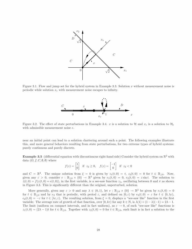
0 x1

x2

x

xe

C

C

D √2

√2

Figure 3.1. Flow and jump set for the hybrid system in Example 3.3. Solution x without measurement noise isperiodic while solution xe with measurement noise escapes to infinity.

]x10

x

xe

C D

Figure 3.2. The effect of state perturbations in Example 3.4. x is a solution to H and xe is a solution to He

with admissible measurement noise e.

near an initial point can lead to a solution chattering around such a point. The following examples illustratethis, and more general behaviors resulting from state perturbations, for two extreme types of hybrid systems:purely continuous and purely discrete.

Example 3.5 (differential equation with discontinuous right-hand side) Consider the hybrid system on R2 with

data (O, f, C, ∅, ∅) where

f(z) =

[10

]if z2 ≥ 0, f(z) =

[−10

]if z2 < 0

and C = R2. The unique solution from ξ = 0 is given by z1(t, 0) = t, z2(t, 0) = 0 for t ∈ R≥0. Now,

given any ε > 0, consider e : R≥0 × 0 → R2 given by e1(t, 0) = 0, e2(t, 0) = ε sin t. The solution to

z(t, 0) = f(z(t, 0) + e(t, 0)), in the first variable, is a see-saw function z1e oscillating between 0 and π as shownin Figure 3.3. This is significantly different than the original, unperturbed, solution.

More generally, given any ε > 0 and any λ ∈ (0, 1), let e : R≥0 × 0 → R2 be given by e1(t, 0) = 0

for t ∈ R≥0 and by e2 that is periodic, with period ε, and defined on [0, ε) by e2(t, 0) = ε for t ∈ [0, λε),e2(t, 0) = −ε for t ∈ [λε, ε). The resulting solution, from ξ = 0, displays a “see-saw like” function in the firstvariable. The average rate of growth of that function, over [0, kε) for any k ∈ N, is λ(1)+ (1−λ)(−1) = 2λ− 1.The limit (uniform on compact intervals, and in fact uniform), as ε → 0, of such “see-saw like” functions isz1(t, 0) = (2λ − 1)t for t ∈ R≥0. Together with z2(t, 0) = 0 for t ∈ R≥0, such limit is in fact a solution to the

28

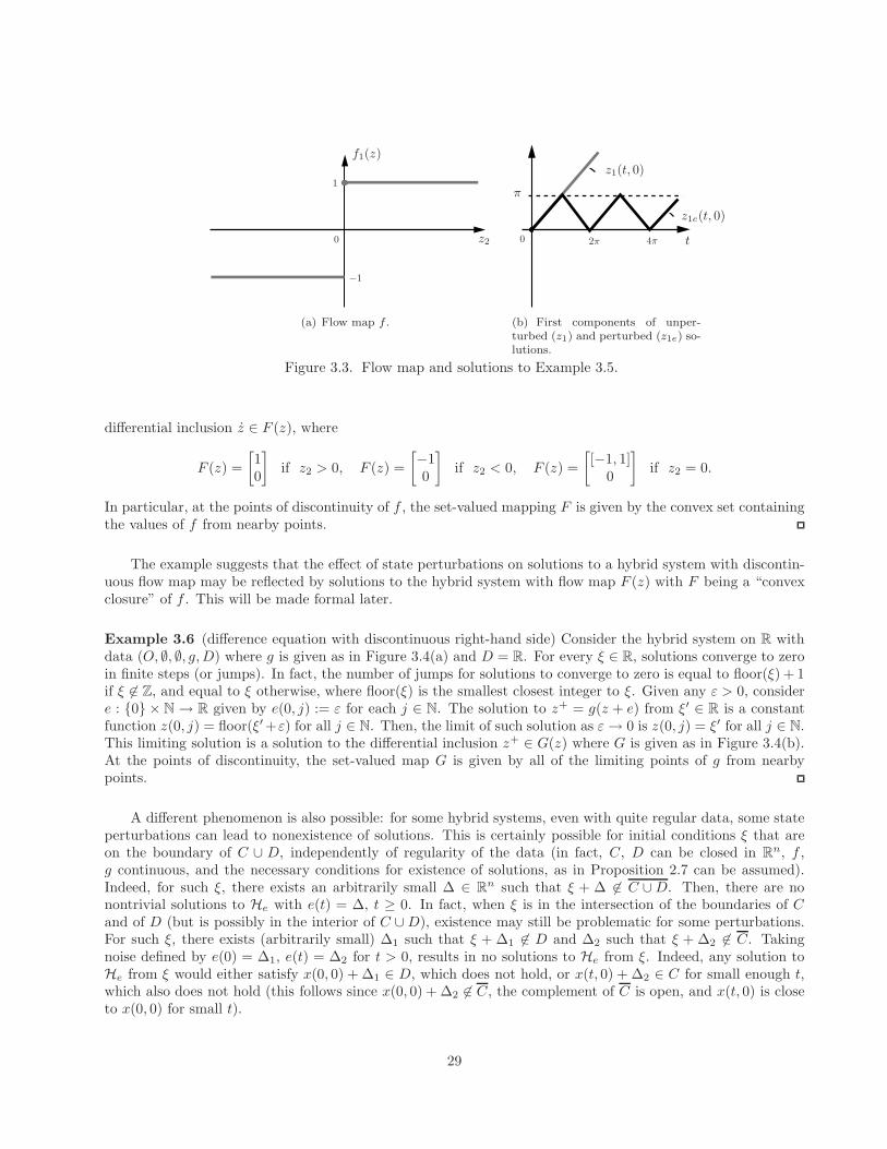
f1(z)

−1

z2

1

0

(a) Flow map f .

π

2π 4π

z1(t, 0)

z1e(t, 0)

t0

(b) First components of unper-turbed (z1) and perturbed (z1e) so-lutions.

Figure 3.3. Flow map and solutions to Example 3.5.

differential inclusion z ∈ F (z), where

F (z) =

[10

]if z2 > 0, F (z) =

[−10

]if z2 < 0, F (z) =

[[−1, 1]

0

]if z2 = 0.

In particular, at the points of discontinuity of f , the set-valued mapping F is given by the convex set containingthe values of f from nearby points.

The example suggests that the effect of state perturbations on solutions to a hybrid system with discontin-uous flow map may be reflected by solutions to the hybrid system with flow map F (z) with F being a “convexclosure” of f . This will be made formal later.

Example 3.6 (difference equation with discontinuous right-hand side) Consider the hybrid system on R withdata (O, ∅, ∅, g,D) where g is given as in Figure 3.4(a) and D = R. For every ξ ∈ R, solutions converge to zeroin finite steps (or jumps). In fact, the number of jumps for solutions to converge to zero is equal to floor(ξ) + 1if ξ 6∈ Z, and equal to ξ otherwise, where floor(ξ) is the smallest closest integer to ξ. Given any ε > 0, considere : 0 × N → R given by e(0, j) := ε for each j ∈ N. The solution to z+ = g(z + e) from ξ′ ∈ R is a constantfunction z(0, j) = floor(ξ′+ε) for all j ∈ N. Then, the limit of such solution as ε→ 0 is z(0, j) = ξ′ for all j ∈ N.This limiting solution is a solution to the differential inclusion z+ ∈ G(z) where G is given as in Figure 3.4(b).At the points of discontinuity, the set-valued map G is given by all of the limiting points of g from nearbypoints.

A different phenomenon is also possible: for some hybrid systems, even with quite regular data, some stateperturbations can lead to nonexistence of solutions. This is certainly possible for initial conditions ξ that areon the boundary of C ∪ D, independently of regularity of the data (in fact, C, D can be closed in R

n, f ,g continuous, and the necessary conditions for existence of solutions, as in Proposition 2.7 can be assumed).Indeed, for such ξ, there exists an arbitrarily small ∆ ∈ R

n such that ξ + ∆ 6∈ C ∪D. Then, there are nonontrivial solutions to He with e(t) = ∆, t ≥ 0. In fact, when ξ is in the intersection of the boundaries of Cand of D (but is possibly in the interior of C ∪D), existence may still be problematic for some perturbations.For such ξ, there exists (arbitrarily small) ∆1 such that ξ + ∆1 6∈ D and ∆2 such that ξ + ∆2 6∈ C. Takingnoise defined by e(0) = ∆1, e(t) = ∆2 for t > 0, results in no solutions to He from ξ. Indeed, any solution toHe from ξ would either satisfy x(0, 0) + ∆1 ∈ D, which does not hold, or x(t, 0) + ∆2 ∈ C for small enough t,which also does not hold (this follows since x(0, 0) + ∆2 6∈ C, the complement of C is open, and x(t, 0) is closeto x(0, 0) for small t).

29

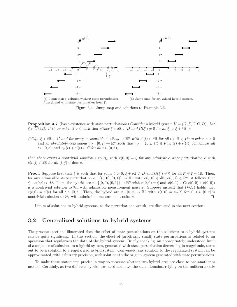
g(z)

zξ ξ′1

1

2

2

3

3

4

4

−1

−1

−2

−2

−3

−3

−4

−4

0

(a) Jump map g, solution without state perturbationfrom ξ, and with state perturbation from ξ′.

G(z)

z1

1

2

2

3

3

4

4

−1

−1

−2

−2

−3

−3

−4

−4

0

(b) Jump map for set-valued hybrid system.

Figure 3.4. Jump map and solutions to Example 3.6.

Proposition 3.7 (basic existence with state perturbations) Consider a hybrid system H = (O,F,C,G,D). Letξ ∈ C ∪D. If there exists δ > 0 such that either ξ + δB ⊂ D and G(ξ′) 6= ∅ for all ξ′ ∈ ξ + δB or

(VCe) ξ + δB ⊂ C and for every measurable e′ : R≥0 → Rn with e′(t) ∈ δB for all t ∈ R≥0 there exists ε > 0

and an absolutely continuous ze′ : [0, ε] → Rn such that ze′ = ξ, ze′(t) ∈ F (ze′(t) + e′(t)) for almost all

t ∈ [0, ε], and ze′(t) + e′(t) ∈ C for all t ∈ (0, ε),

then there exists a nontrivial solution x to He with x(0, 0) = ξ for any admissible state perturbation e withe(t, j) ∈ δB for all (t, j) ∈ dom e.

Proof. Suppose first that ξ is such that for some δ > 0, ξ + δB ⊂ D and G(ξ′) 6= ∅ for all ξ′ ∈ ξ + δB. Then,for any admissible state perturbation e : (0, 0), (0, 1) → R

n with e(0, 0) ∈ δB, e(0, 1) ∈ Rn, it follows that

ξ + e(0, 0) ∈ D. Then, the hybrid arc x : (0, 0), (0, 1) → Rn with x(0, 0) = ξ and x(0, 1) ∈ G(x(0, 0) + e(0, 0))

is a nontrivial solution to He with admissible measurement noise e. Suppose instead that (VCe) holds. Lete(t, 0) = e′(t) for all t ∈ [0, ε]. Then, the hybrid arc x : [0, ε] → R

n with x(t, 0) = ze′(t) for all t ∈ [0, ε] isnontrivial solution to He with admissible measurement noise e.

Limits of solutions to hybrid systems, as the perturbations vanish, are discussed in the next section.

3.2 Generalized solutions to hybrid systems

The previous sections illustrated that the effect of state perturbations on the solutions to a hybrid systemscan be quite significant. In this section, the effect of (arbitrarily small) state perturbations is related to anoperation that regularizes the data of the hybrid system. Briefly speaking, an appropriately understood limitof a sequence of solutions to a hybrid system, generated with state perturbation decreasing in magnitude, turnsout to be a solution to a regularized hybrid system. Conversely, any solution to the regularized system can beapproximated, with arbitrary precision, with solutions to the original system generated with state perturbations.

To make these statements precise, a way to measure whether two hybrid arcs are close to one another isneeded. Certainly, as two different hybrid arcs need not have the same domains, relying on the uniform metric

30

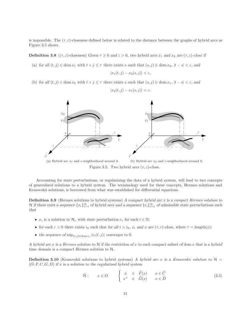
is impossible. The (τ, ε)-closeness defined below is related to the distance between the graphs of hybrid arcs asFigure 3.5 shows.

Definition 3.8 ((τ, ε)-closeness) Given τ ≥ 0 and ε > 0, two hybrid arcs x1 and x2 are (τ, ε)-close if

(a) for all (t, j) ∈ domx1 with t+ j ≤ τ there exists s such that (s, j) ∈ domx2, |t− s| < ε, and

|x1(t, j) − x2(s, j)| < ε,

(b) for all (t, j) ∈ domx2 with t+ j ≤ τ there exists s such that (s, j) ∈ domx1, |t− s| < ε, and

|x2(t, j) − x1(s, j)| < ε.

x2

x1

j

t

τ

1

0

(a) Hybrid arc x1 and ε-neighborhood around it.

x2

x1

j

t

τ

1

0

(b) Hybrid arc x2 and ε-neighborhood around it.

Figure 3.5. Two hybrid arcs (τ, ε)-close.

Accounting for state perturbations, or regularizing the data of a hybrid system, will lead to two conceptsof generalized solutions to a hybrid system. The terminology used for these concepts, Hermes solutions andKrasovskii solutions, is borrowed from what was established for differential equations.

Definition 3.9 (Hermes solutions to hybrid systems) A compact hybrid arc x is a compact Hermes solution toH if there exist a sequence xi∞i=1 of hybrid arcs and a sequence ei∞i=1 of admissible state perturbations suchthat

• xi is a solution to He with state perturbation ei for each i ∈ N;

• for each ε > 0 there exists i0 such that for all i > i0, xi and x are (τ, ε)-close, where τ = length(x);

• the sequence of sup(t,j)∈dom ei|ei(t, j)| converges to 0.

A hybrid arc x is a Hermes solution to H if the restriction of x to each compact subset of domx that is a hybridtime domain is a compact Hermes solution to H.

Definition 3.10 (Krasovskii solutions to hybrid systems) A hybrid arc x is a Krasovskii solution to H =(O,F,C,G,D) if x is a solution to the regularized hybrid system

H : x ∈ O

x ∈ F (x) x ∈ C

x+ ∈ G(x) x ∈ D(3.5)

31

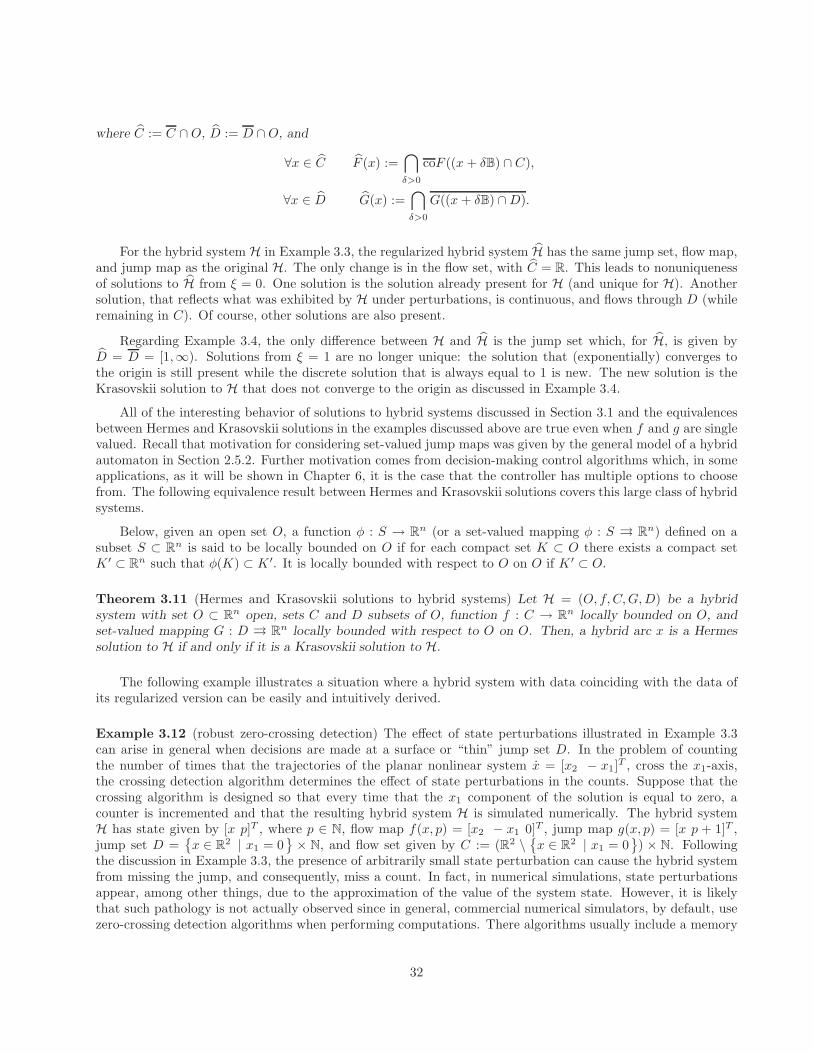
where C := C ∩O, D := D ∩O, and

∀x ∈ C F (x) :=⋂

δ>0

coF ((x + δB) ∩ C),

∀x ∈ D G(x) :=⋂

δ>0

G((x + δB) ∩D).

For the hybrid system H in Example 3.3, the regularized hybrid system H has the same jump set, flow map,and jump map as the original H. The only change is in the flow set, with C = R. This leads to nonuniquenessof solutions to H from ξ = 0. One solution is the solution already present for H (and unique for H). Anothersolution, that reflects what was exhibited by H under perturbations, is continuous, and flows through D (whileremaining in C). Of course, other solutions are also present.

Regarding Example 3.4, the only difference between H and H is the jump set which, for H, is given byD = D = [1,∞). Solutions from ξ = 1 are no longer unique: the solution that (exponentially) converges tothe origin is still present while the discrete solution that is always equal to 1 is new. The new solution is theKrasovskii solution to H that does not converge to the origin as discussed in Example 3.4.

All of the interesting behavior of solutions to hybrid systems discussed in Section 3.1 and the equivalencesbetween Hermes and Krasovskii solutions in the examples discussed above are true even when f and g are singlevalued. Recall that motivation for considering set-valued jump maps was given by the general model of a hybridautomaton in Section 2.5.2. Further motivation comes from decision-making control algorithms which, in someapplications, as it will be shown in Chapter 6, it is the case that the controller has multiple options to choosefrom. The following equivalence result between Hermes and Krasovskii solutions covers this large class of hybridsystems.

Below, given an open set O, a function φ : S → Rn (or a set-valued mapping φ : S →→ R

n) defined on asubset S ⊂ R

n is said to be locally bounded on O if for each compact set K ⊂ O there exists a compact setK ′ ⊂ R

n such that φ(K) ⊂ K ′. It is locally bounded with respect to O on O if K ′ ⊂ O.

Theorem 3.11 (Hermes and Krasovskii solutions to hybrid systems) Let H = (O, f, C,G,D) be a hybridsystem with set O ⊂ R

n open, sets C and D subsets of O, function f : C → Rn locally bounded on O, and

set-valued mapping G : D →→ Rn locally bounded with respect to O on O. Then, a hybrid arc x is a Hermes

solution to H if and only if it is a Krasovskii solution to H.

The following example illustrates a situation where a hybrid system with data coinciding with the data ofits regularized version can be easily and intuitively derived.

Example 3.12 (robust zero-crossing detection) The effect of state perturbations illustrated in Example 3.3can arise in general when decisions are made at a surface or “thin” jump set D. In the problem of countingthe number of times that the trajectories of the planar nonlinear system x = [x2 − x1]

T , cross the x1-axis,the crossing detection algorithm determines the effect of state perturbations in the counts. Suppose that thecrossing algorithm is designed so that every time that the x1 component of the solution is equal to zero, acounter is incremented and that the resulting hybrid system H is simulated numerically. The hybrid systemH has state given by [x p]T , where p ∈ N, flow map f(x, p) = [x2 − x1 0]T , jump map g(x, p) = [x p + 1]T ,jump set D =

x ∈ R

2 | x1 = 0× N, and flow set given by C := (R2 \

x ∈ R

2 | x1 = 0) × N. Following

the discussion in Example 3.3, the presence of arbitrarily small state perturbation can cause the hybrid systemfrom missing the jump, and consequently, miss a count. In fact, in numerical simulations, state perturbationsappear, among other things, due to the approximation of the value of the system state. However, it is likelythat such pathology is not actually observed since in general, commercial numerical simulators, by default, usezero-crossing detection algorithms when performing computations. There algorithms usually include a memory

32

variable that keeps track of the side of the decision boundary in which the state is located. Such an algorithmcan be modeled with the following hybrid system with the state space O = R

4:

f(x, p, q) :=

[x2

−x1

]

00

, C :=

(x, p, q) ∈ R

2 × N × −1, 1 | x1q ≥ 0

g(x, p, q) :=

x

p+ 1−sign(x1)

, D := ∪q∈−1,1(Dq × N × q)

where sign(r) = −1 if r < 0, 1 if r > 0, and −1, 1 if r = 0; D1 :=x ∈ R

2 | x1 ≥ 0, x2 = 0; and D−1 :=

x ∈ R2 | x1 ≤ 0, x2 = 0

. It follows that this hybrid system and its regularization coincide. Then, state

perturbations do not affect the number of crosses of the x1-axis. Figure 3.6 illustrates solutions to H and thishybrid system with state perturbations.

C

C

x(0, 0)

D

x1

x2

(a) Solutions with state perturbationsmay miss counts when state perturba-tions are present.

D1

D−1

C

C

x(0, 0)

q = 1

q = −1

x1

x1

x2

x2

(b) Solutions with robust zero-crossingdetection: flows are not possible anylonger once the jump set is crossed,which forces q to jump and register acount.

Figure 3.6. Solutions to zero-crossing detection system in Example 3.12.

33

3.3 Measurement noise in feedback control

In general feedback control systems, hybrid or not, measurement noise enters the system not as a state per-turbation affecting every occurrence of the state in the equations of motion, but only through feedback. Morespecifically, given a general nonlinear control system z = φ(z, u) and a feedback mapping u = κ(z) (cer-tain control objectives require the use of discontinuous feedback κ), measurement noise enters the closed loopz = φ(z, κ(z)) through the feedback, leading to differential equations like z = φ(z, κ(z+ e)). When the feedbackis hybrid, or when the control system is hybrid to begin with, the measurement error can also interplay withthe flow sets, jump sets, and the jump map. Some of this is illustrated in the following example.

Example 3.13 (robust stabilization and measurement noise) Consider a simple control system z = u withz ∈ R, u ∈ [−1, 1]. The goal is to robustly stabilize the set consisting of two points: A = 0, 6 via feedback.Let sat : R → [−1, 1] be the standard saturation function, that is

sat(u) = −1 if u < −1, sat(u) = u if u ∈ [−1, 1], sat(u) = 1 if u > 1.

A nonhybrid feedback that results in asymptotic stability of A for the closed loop z = k(z), and that closed-loopsystem are described below:

z = k(z) :=

−sat(z) if z ≤ 3

−sat(z − 6) if z > 3 .

Note that this k is discontinuous at z = 3, and because of this, the resulting asymptotic stability is not robustto measurement noise. Indeed, for arbitrarily small ε > 0, the unique solution from 3 to z = k(z + e) withe(t) := ε cos(πt/ε) is a see-saw function oscillating between 3 − ε and 3 + ε with period 2ε. The uniform limitof such see-saw functions is a constant function z(t) = 3 for all t ∈ R≥0. Of course, the nonrobustness ofasymptotic stability can be detected by looking for Krasovskii solutions to z = k(z). These are the solutionsto the differential inclusion z ∈ K(z), where K differs from k only at the point of discontinuity of k, thatis, K(3) = [−1, 1]. Obviously, 3 is an equilibrium of z ∈ K(z). (And so the constant function z(t) = 3 is aKrasovskii solution to z = f(z), and equivalently, a Hermes solution. That the constant function is a Hermessolution can be seen directly, as it is the uniform limit, as εց 0, of the see-saw functions constructed above.)

Asymptotic stability of A that is robust to measurement noise can be accomplished by hybrid feedback.One possible approach is based on hysteresis, with the hybrid feedback involving an additional logic variableq ∈ 1, 2. To make an analogy with the nonhybrid feedback analyzed above, the logic variable will, in a sense,keep track of whether z ≤ 3 or z > 3, and will prohibit switching between these two instances too often. Morespecifically, the hybrid feedback will set u = −sat(z) if the logic variable q equals 1 and z ≤ 4, and will setu = −sat(z − 6) if q = 2 and z ≥ 2. If neither of the conditions is met, the logic variable q will be toggled. Inclosed loop, this leads to a hybrid system H in R

2 with the flow and jump sets

C = (−∞, 4] × 1 ∪ [2,∞) × 2, D = (4,∞) × 1 ∪ (−∞, 2) × 2,

and the flow and jump equations given by

z = f(z, q) :=

−sat(z) if (z, 1) ∈ C

−sat(z − 6) if (z, 2) ∈ C, q+ = g(q) = 3 − q.

The logic variable q remains constant during flow, and the state z remains constant during jumps. Figure 3.7depicts the flow and jump sets and two solutions. It is easy to verify that solutions x = (z, q) to H jump atmost once, the maximal ones are complete, and the set A× 1, 2 is globally uniformly asymptotically stable.The solutions are also unique for any initial condition. The uniqueness would no longer be true if the jump setD was replaced by its closure. Indeed, then a solution from (4, 1) could only flow (with z converging to 0) orjump first (with q changing from 1 to 2) and then flow (with z converging to 6). Similar nonuniqueness wouldalso occur from (2, 2). Still, such nonuniqueness does not affect asymptotic stability.

34

]

]

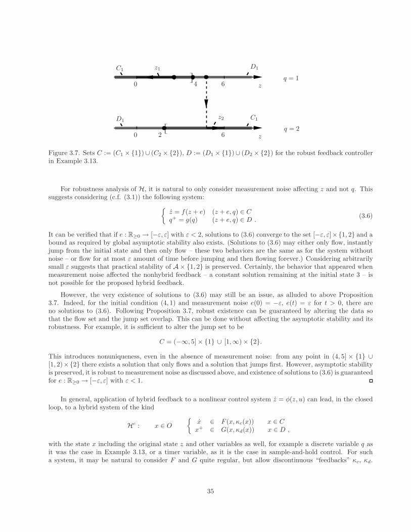
q = 1

q = 2z

z

z1

z2

6

64

20

0

C1

C1

D1

D1

Figure 3.7. Sets C := (C1 × 1)∪ (C2 × 2), D := (D1 × 1)∪ (D2 × 2) for the robust feedback controllerin Example 3.13.

For robustness analysis of H, it is natural to only consider measurement noise affecting z and not q. Thissuggests considering (c.f. (3.1)) the following system:

z = f(z + e) (z + e, q) ∈ Cq+ = g(q) (z + e, q) ∈ D .

(3.6)

It can be verified that if e : R≥0 → [−ε, ε] with ε < 2, solutions to (3.6) converge to the set [−ε, ε]×1, 2 and abound as required by global asymptotic stability also exists. (Solutions to (3.6) may either only flow, instantlyjump from the initial state and then only flow – these two behaviors are the same as for the system withoutnoise – or flow for at most ε amount of time before jumping and then flowing forever.) Considering arbitrarilysmall ε suggests that practical stability of A× 1, 2 is preserved. Certainly, the behavior that appeared whenmeasurement noise affected the nonhybrid feedback – a constant solution remaining at the initial state 3 – isnot possible for the proposed hybrid feedback.

However, the very existence of solutions to (3.6) may still be an issue, as alluded to above Proposition3.7. Indeed, for the initial condition (4, 1) and measurement noise e(0) = −ε, e(t) = ε for t > 0, there areno solutions to (3.6). Following Proposition 3.7, robust existence can be guaranteed by altering the data sothat the flow set and the jump set overlap. This can be done without affecting the asymptotic stability and itsrobustness. For example, it is sufficient to alter the jump set to be

C = (−∞, 5] × 1 ∪ [1,∞) × 2.

This introduces nonuniqueness, even in the absence of measurement noise: from any point in (4, 5] × 1 ∪[1, 2)×2 there exists a solution that only flows and a solution that jumps first. However, asymptotic stabilityis preserved, it is robust to measurement noise as discussed above, and existence of solutions to (3.6) is guaranteedfor e : R≥0 → [−ε, ε] with ε < 1.

In general, application of hybrid feedback to a nonlinear control system z = φ(z, u) can lead, in the closedloop, to a hybrid system of the kind

Hc : x ∈ O

x ∈ F (x, κc(x)) x ∈ Cx+ ∈ G(x, κd(x)) x ∈ D ,

with the state x including the original state z and other variables as well, for example a discrete variable q asit was the case in Example 3.13, or a timer variable, as it is the case in sample-and-hold control. For sucha system, it may be natural to consider F and G quite regular, but allow discontinuous “feedbacks” κc, κd.

35

Assuming that the measurement error enters Hc through the mappings κc, κd and also affects the flow and thejump sets, leads to the system

Hce : x+ e ∈ O

x ∈ F (x, κc(x+ e)) x+ e ∈ Cx+ ∈ G(x, κd(x + e)) x+ e ∈ D .

Two notions of generalized solutions to Hc above can be considered, paralleling the notions of Hermes solutionsand Krasovskii solutions in Definitions 3.9 and 3.10. Control Hermes solutions can be defined as limits ofsequences of solutions to Hc

e generated with sequences of measurement noise vanishing in the limit.

Definition 3.14 (Control Hermes solutions to hybrid systems) A compact hybrid arc x is a compact controlHermes solution to H if there exist a sequence xi∞i=1 of hybrid arcs and a sequence ei∞i=1 of admissible stateperturbations such that

• xi is a solution to He (with flow map condition F (x, κc(x+ e)) and jump map condition G(x, κd(x+ e)))with state perturbation ei for each i ∈ N;

• for each ε > 0 there exists i0 such that for all i > i0, xi and x are (τ, ε)-close, where τ = length(x);

• the sequence of sup(t,j)∈dom ei|ei(t, j)| converges to 0.

A hybrid arc x is a control Hermes solution to H if the restriction of x to each compact subset of domx that isa hybrid time domain is a compact control Hermes solution to H.

Control Krasovskii solutions can be defined as just Krasovskii solutions, as in Definition 3.9. (While aseemingly different approach would be to consider x ∈ ∩δ>0coF (x, κc((x + δB) ∩ C)) and a similarly definedjump equation, mild regularity – including continuity – of F and just local boundedness – but not continuity –of κc make such an approach lead to Krasovskii solutions.) Equivalences between control Hermes and Krasovskiisolutions to Hc as in Theorem 3.11 can be also shown. This is stated below.

Corollary 3.15 (control Hermes and Krasovskii solutions to hybrid systems) Let H = (O, f, C, g,D) be ahybrid system with set O ⊂ R

n open; sets C and D subsets of O; function f : O × Rmc → R

n locally Lipschitzcontinuous in the first argument, locally uniformly in the second argument 1. ; function g : O × R

md → Ocontinuous in the first argument, locally uniformly in the second argument; and functions κc : C → R

mc ,κd : D → R

md locally bounded on O. Then a hybrid arc x is a control Hermes solution to Hc if and only if itis a Krasovskii solution to Hc.

The following feedback control examples illustrate the relevance of generalized solutions in robust stabiliza-tion.

Example 3.16 (impulsive and reset control systems) State-dependent impulsive systems are dynamical systemswith states that jump when a condition of the state is satisfied, and flow otherwise. State-dependent impulsivesystems are generally modeled as

x = f(x) := fc(x) x 6∈ Mx+ = g(x) := x+ fd(x) x ∈ M

1A function h : O×Rm → R

n is continuous (locally Lipschitz continuous) in the first argument, locally uniformly in the secondargument if for each z ∈ O, each compact U ⊂ R

m, and each ε > 0 there exists δ > 0 (K > 0) such that |x − z| < δ implies|h(x, u) − h(z, u)| < ε (x, y ∈ (z + εB) ∩O implies |h(x, u) − h(y, u)| ≤ K|x− y|) for all u ∈ U .

36

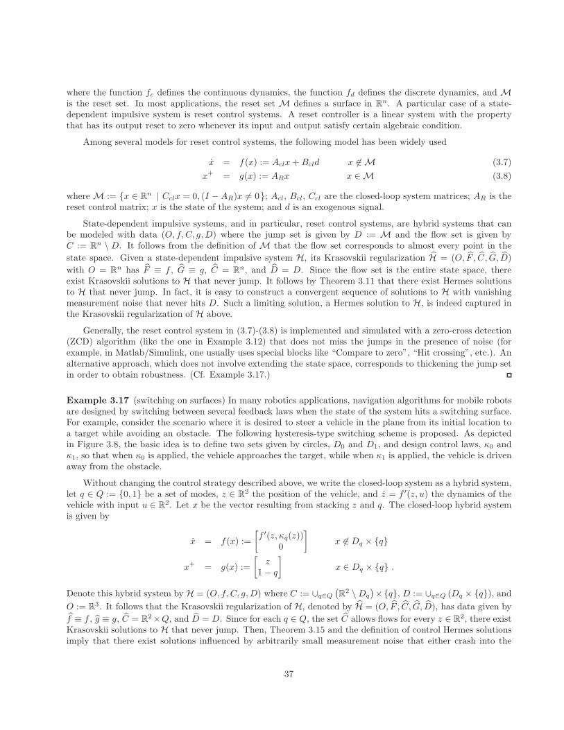
where the function fc defines the continuous dynamics, the function fd defines the discrete dynamics, and Mis the reset set. In most applications, the reset set M defines a surface in R

n. A particular case of a state-dependent impulsive system is reset control systems. A reset controller is a linear system with the propertythat has its output reset to zero whenever its input and output satisfy certain algebraic condition.

Among several models for reset control systems, the following model has been widely used

x = f(x) := Aclx+Bcld x 6∈ M (3.7)

x+ = g(x) := ARx x ∈ M (3.8)

where M := x ∈ Rn | Cclx = 0, (I −AR)x 6= 0; Acl, Bcl, Ccl are the closed-loop system matrices; AR is the

reset control matrix; x is the state of the system; and d is an exogenous signal.

State-dependent impulsive systems, and in particular, reset control systems, are hybrid systems that canbe modeled with data (O, f, C, g,D) where the jump set is given by D := M and the flow set is given byC := R

n \ D. It follows from the definition of M that the flow set corresponds to almost every point in the

state space. Given a state-dependent impulsive system H, its Krasovskii regularization H = (O, F , C, G, D)

with O = Rn has F ≡ f , G ≡ g, C = R

n, and D = D. Since the flow set is the entire state space, thereexist Krasovskii solutions to H that never jump. It follows by Theorem 3.11 that there exist Hermes solutionsto H that never jump. In fact, it is easy to construct a convergent sequence of solutions to H with vanishingmeasurement noise that never hits D. Such a limiting solution, a Hermes solution to H, is indeed captured inthe Krasovskii regularization of H above.

Generally, the reset control system in (3.7)-(3.8) is implemented and simulated with a zero-cross detection(ZCD) algorithm (like the one in Example 3.12) that does not miss the jumps in the presence of noise (forexample, in Matlab/Simulink, one usually uses special blocks like “Compare to zero”, “Hit crossing”, etc.). Analternative approach, which does not involve extending the state space, corresponds to thickening the jump setin order to obtain robustness. (Cf. Example 3.17.)

Example 3.17 (switching on surfaces) In many robotics applications, navigation algorithms for mobile robotsare designed by switching between several feedback laws when the state of the system hits a switching surface.For example, consider the scenario where it is desired to steer a vehicle in the plane from its initial location toa target while avoiding an obstacle. The following hysteresis-type switching scheme is proposed. As depictedin Figure 3.8, the basic idea is to define two sets given by circles, D0 and D1, and design control laws, κ0 andκ1, so that when κ0 is applied, the vehicle approaches the target, while when κ1 is applied, the vehicle is drivenaway from the obstacle.

Without changing the control strategy described above, we write the closed-loop system as a hybrid system,let q ∈ Q := 0, 1 be a set of modes, z ∈ R

2 the position of the vehicle, and z = f ′(z, u) the dynamics of thevehicle with input u ∈ R

2. Let x be the vector resulting from stacking z and q. The closed-loop hybrid systemis given by

x = f(x) :=

[f ′(z, κq(z))

0

]x 6∈ Dq × q

x+ = g(x) :=

[z

1 − q

]x ∈ Dq × q .

Denote this hybrid system by H = (O, f, C, g,D) where C := ∪q∈Q

(R

2 \Dq

)×q, D := ∪q∈Q (Dq × q), and

O := R3. It follows that the Krasovskii regularization of H, denoted by H = (O, F , C, G, D), has data given by

f ≡ f , g ≡ g, C = R2×Q, and D = D. Since for each q ∈ Q, the set C allows flows for every z ∈ R

2, there existKrasovskii solutions to H that never jump. Then, Theorem 3.15 and the definition of control Hermes solutionsimply that there exist solutions influenced by arbitrarily small measurement noise that either crash into the

37

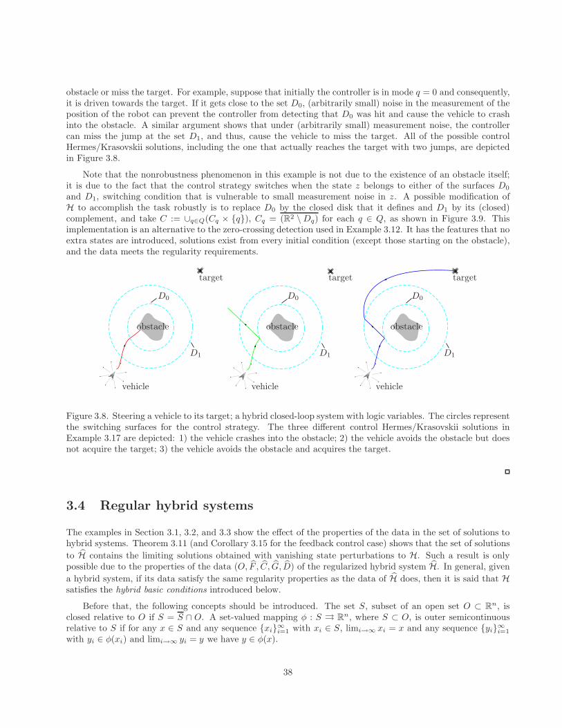
obstacle or miss the target. For example, suppose that initially the controller is in mode q = 0 and consequently,it is driven towards the target. If it gets close to the set D0, (arbitrarily small) noise in the measurement of theposition of the robot can prevent the controller from detecting that D0 was hit and cause the vehicle to crashinto the obstacle. A similar argument shows that under (arbitrarily small) measurement noise, the controllercan miss the jump at the set D1, and thus, cause the vehicle to miss the target. All of the possible controlHermes/Krasovskii solutions, including the one that actually reaches the target with two jumps, are depictedin Figure 3.8.

Note that the nonrobustness phenomenon in this example is not due to the existence of an obstacle itself;it is due to the fact that the control strategy switches when the state z belongs to either of the surfaces D0

and D1, switching condition that is vulnerable to small measurement noise in z. A possible modification ofH to accomplish the task robustly is to replace D0 by the closed disk that it defines and D1 by its (closed)complement, and take C := ∪q∈Q(Cq × q), Cq = (R2 \Dq) for each q ∈ Q, as shown in Figure 3.9. Thisimplementation is an alternative to the zero-crossing detection used in Example 3.12. It has the features that noextra states are introduced, solutions exist from every initial condition (except those starting on the obstacle),and the data meets the regularity requirements.

targettargettarget

vehiclevehiclevehicle

D0D0D0

D1D1D1

obstacleobstacleobstacle

Figure 3.8. Steering a vehicle to its target; a hybrid closed-loop system with logic variables. The circles representthe switching surfaces for the control strategy. The three different control Hermes/Krasovskii solutions inExample 3.17 are depicted: 1) the vehicle crashes into the obstacle; 2) the vehicle avoids the obstacle but doesnot acquire the target; 3) the vehicle avoids the obstacle and acquires the target.

3.4 Regular hybrid systems

The examples in Section 3.1, 3.2, and 3.3 show the effect of the properties of the data in the set of solutions tohybrid systems. Theorem 3.11 (and Corollary 3.15 for the feedback control case) shows that the set of solutions

to H contains the limiting solutions obtained with vanishing state perturbations to H. Such a result is onlypossible due to the properties of the data (O, F , C, G, D) of the regularized hybrid system H. In general, given

a hybrid system, if its data satisfy the same regularity properties as the data of H does, then it is said that Hsatisfies the hybrid basic conditions introduced below.

Before that, the following concepts should be introduced. The set S, subset of an open set O ⊂ Rn, is

closed relative to O if S = S ∩ O. A set-valued mapping φ : S →→ Rn, where S ⊂ O, is outer semicontinuous

relative to S if for any x ∈ S and any sequence xi∞i=1 with xi ∈ S, limi→∞ xi = x and any sequence yi∞i=1

with yi ∈ φ(xi) and limi→∞ yi = y we have y ∈ φ(x).

38

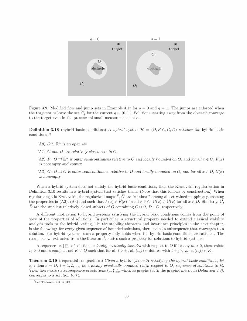
targettarget

D0

D1C0

C1

obstacleobstacle

q = 0 q = 1

Figure 3.9. Modified flow and jump sets in Example 3.17 for q = 0 and q = 1. The jumps are enforced whenthe trajectories leave the set Cq for the current q ∈ 0, 1. Solutions starting away from the obstacle convergeto the target even in the presence of small measurement noise.

Definition 3.18 (hybrid basic conditions) A hybrid system H = (O,F,C,G,D) satisfies the hybrid basicconditions if

(A0) O ⊂ Rn is an open set.

(A1) C and D are relatively closed sets in O.

(A2) F : O →→ Rn is outer semicontinuous relative to C and locally bounded on O, and for all x ∈ C, F (x)

is nonempty and convex.

(A3) G : O →→ O is outer semicontinuous relative to D and locally bounded on O, and for all x ∈ D, G(x)is nonempty.

When a hybrid system does not satisfy the hybrid basic conditions, then the Krasovskii regularization inDefinition 3.10 results in a hybrid system that satisfies them. (Note that this follows by construction.) When

regularizing a la Krasovskii, the regularized maps F , G are “minimal” among all set-valued mappings possessingthe properties in (A2), (A3) and such that F (x) ∈ F (x) for all x ∈ C, G(x) ⊂ G(x) for all x ∈ D. Similarly, C,

D are the smallest relatively closed subsets of O containing C ∩O, D ∩O, respectively.

A different motivation to hybrid systems satisfying the hybrid basic conditions comes from the point ofview of the properties of solutions. In particular, a structural property needed to extend classical stabilityanalysis tools to the hybrid setting, like the stability theorems and invariance principles in the next chapter,is the following: for every given sequence of bounded solutions, there exists a subsequence that converges to asolution. For hybrid systems, such a property only holds when the hybrid basic conditions are satisfied. Theresult below, extracted from the literature2, states such a property for solutions to hybrid systems.

A sequence xi∞i=1 of solutions is locally eventually bounded with respect to O if for any m > 0, there existsi0 > 0 and a compact set K ⊂ O such that for all i > i0, all (t, j) ∈ domxi with t+ j < m, xi(t, j) ∈ K.

Theorem 3.19 (sequential compactness) Given a hybrid system H satisfying the hybrid basic conditions, letxi : domx → O, i = 1, 2, . . ., be a locally eventually bounded (with respect to O) sequence of solutions to H.Then there exists a subsequence of solutions xi∞i=0 which as graphs (with the graphic metric in Definition 3.8),converges to a solution to H.

2See Theorem 4.4 in [39].

39

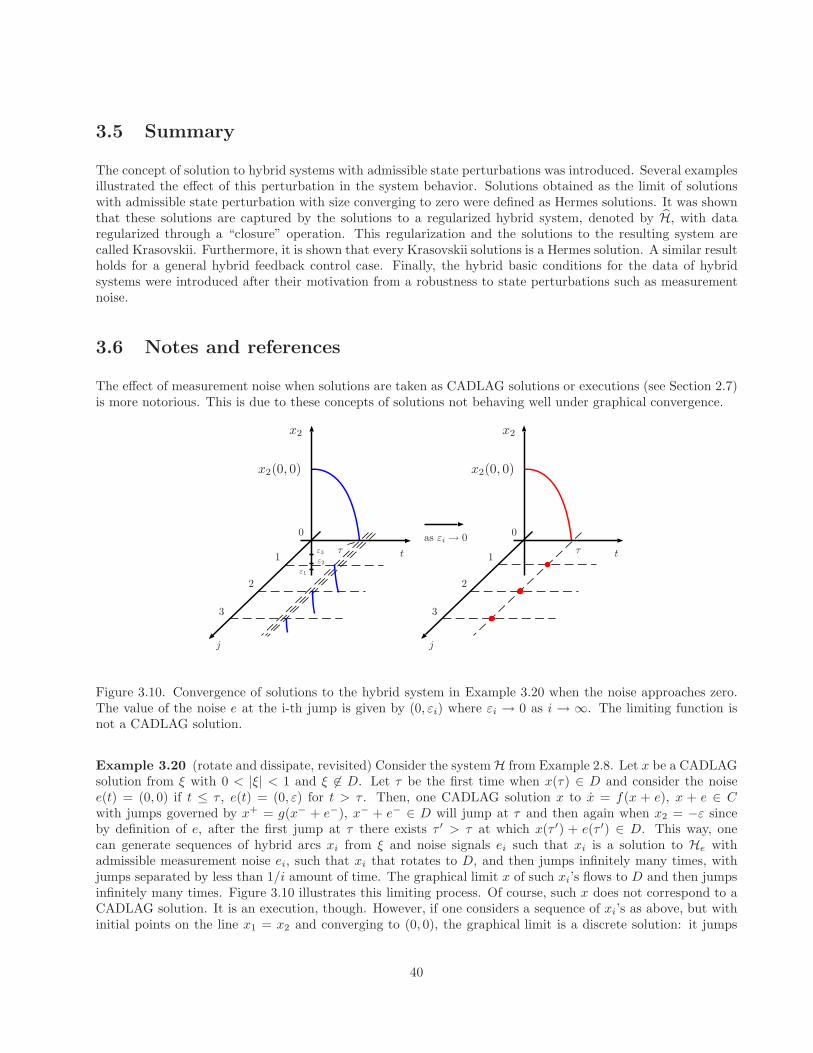
3.5 Summary

The concept of solution to hybrid systems with admissible state perturbations was introduced. Several examplesillustrated the effect of this perturbation in the system behavior. Solutions obtained as the limit of solutionswith admissible state perturbation with size converging to zero were defined as Hermes solutions. It was shownthat these solutions are captured by the solutions to a regularized hybrid system, denoted by H, with dataregularized through a “closure” operation. This regularization and the solutions to the resulting system arecalled Krasovskii. Furthermore, it is shown that every Krasovskii solutions is a Hermes solution. A similar resultholds for a general hybrid feedback control case. Finally, the hybrid basic conditions for the data of hybridsystems were introduced after their motivation from a robustness to state perturbations such as measurementnoise.


The effect of measurement noise when solutions are taken as CADLAG solutions or executions (see Section 2.7)is more notorious. This is due to these concepts of solutions not behaving well under graphical convergence.

0 0

1 1

2 2

3 3

t t

j j

τ τas εi → 0

ε3ε2

ε1

x2 x2

x2(0, 0) x2(0, 0)

Figure 3.10. Convergence of solutions to the hybrid system in Example 3.20 when the noise approaches zero.The value of the noise e at the i-th jump is given by (0, εi) where εi → 0 as i → ∞. The limiting function isnot a CADLAG solution.

Example 3.20 (rotate and dissipate, revisited) Consider the system H from Example 2.8. Let x be a CADLAGsolution from ξ with 0 < |ξ| < 1 and ξ 6∈ D. Let τ be the first time when x(τ) ∈ D and consider the noisee(t) = (0, 0) if t ≤ τ , e(t) = (0, ε) for t > τ . Then, one CADLAG solution x to x = f(x + e), x + e ∈ Cwith jumps governed by x+ = g(x− + e−), x− + e− ∈ D will jump at τ and then again when x2 = −ε sinceby definition of e, after the first jump at τ there exists τ ′ > τ at which x(τ ′) + e(τ ′) ∈ D. This way, onecan generate sequences of hybrid arcs xi from ξ and noise signals ei such that xi is a solution to He withadmissible measurement noise ei, such that xi that rotates to D, and then jumps infinitely many times, withjumps separated by less than 1/i amount of time. The graphical limit x of such xi’s flows to D and then jumpsinfinitely many times. Figure 3.10 illustrates this limiting process. Of course, such x does not correspond to aCADLAG solution. It is an execution, though. However, if one considers a sequence of xi’s as above, but withinitial points on the line x1 = x2 and converging to (0, 0), the graphical limit is a discrete solution: it jumps

40

infinitely many times from (0, 0) to (0, 0) with no intervals of flow. While such limit is a hybrid arc, it is not anexecution of H since (0, 0) 6∈ D. By definition, it is a Hermes solution.

The following example connects the regularization of the hybrid systems introduced in this chapter withExample 2.8 and the example above.

Example 3.21 (rotate and dissipate, re-revisited) Consider the system H from Example 2.8. The regularized

hybrid system H with O = R2 has data given by C = R

2, D = [0, 1] × 0, while f ≡ f , g ≡ g. In particular,there exists a discrete Krasovskii solution given by x(0, j) = [0 0]T for all j ∈ N. As we noted in Example 3.20,this is also a Hermes solution to H, but is not an execution of H. Another way that Krasovskii solutions differfrom executions is that there are Krasovskii solutions from initial points ξ with |ξ| = 1 that flow and then jump

(as [1 0]T ∈ D) while the unique execution from ξ only flows.

The regularization for F follows the Krasovskii regularization for discontinuous right-hand sides introducedin [55] (see also [42]). It differs from the Filippov’s regularization [36] as this ignores the behavior of the right-hand side on sets of measure zero. Such a regularization technique proves to be unsuitable for hybrid systems(and even for constrained differential equations). Indeed, for example, a set C with zero measure leads toan “empty” regularization. For further details on the relationship of regularized to unregularized right-handsides see [36], [44], [55], and [42]. Regarding G, the regularization follows the one used in [52] for single-valuedright-hand sides; due to the nature of discrete time, the convexification is not needed.

Theorem 3.11 and Corollary 3.15 are generalizations to the hybrid setting of a result for differential equationsinitially reported by Hermes in [44] and expanded upon by Hajek in [42] and a result by Coron and Rosier [31]given in the context of robust stabilization of nonlinear control systems (with non-hybrid feedback), respectively.As a special case, they subsume analogous results for difference equations. These generalizations are enabledboth by the novel concept of solution to hybrid systems and the use of graphical convergence, rather thanpointwise, of sequences of solutions.

To be consistent with what is encountered in hybrid feedback control design, the equivalence result inCorollary 3.15 did not allow for the control functions κc and κd to be set valued. However, this can be easilyadjusted to account for a set-valued version of this functions. Similarly, Theorem 3.11 can be adjusted to allowfor a set-valued flow map.

One of the earliest references dealing with impulsive systems as in Example 3.16 is the work by Bainovand Simeonov [11]. The general model in that example follows the model in [25]. Regarding reset controlsystems, the first reset integrator was introduced in [29] in order to improve the performance of linear systems.Subsequent efforts in studying the stability properties of reset control include [56], [12], [106]. The particularmodel for reset control systems in Example 3.16 follows the model in [12].

Example 3.6 is borrowed from [52]. Example 3.13 was suggested by Rafal Goebel.

The robotic problem and hysteresis control strategy in Example 3.17 was taken from [13, Section 3].

Theorem 3.19 appeared as Theorem 4.4 in [39]. The proofs of Theorem 3.11 and Corollary 3.15 can befound in Section B.1.

41

Chapter 4

Stability and Invariance

In this chapter, stability theorems and invariance principles for hybrid systems are developed. These resultsprovide a methodical procedure to establish stability and asymptotic stability of compact sets, and to obtaininformation about the convergence properties of solutions to hybrid systems. Examples throughout the chapterillustrate the concepts and results.

4.1 Stability

4.1.1 Definitions

The concept of stability for hybrid systems H is now introduced. They parallel the standard notions forcontinuous and discrete-time systems. The prefix “pre” in the definitions below is used to indicate that maximalsolutions, that is, the elements in SH, are not necessarily complete. In fact, in the case that every maximalsolution is complete, the prefix “pre” can be dropped. For instance, this is the case when in addition to(A0)-(A4), it is true that (VC) (see Proposition 2.7) and

(VD) for each ξ ∈ D, G(ξ) ⊂ C ∪D

hold. (Under conditions (VC) and (VD), any maximal solution to H is either complete or eventually leaves anycompact subset of O.)

Definition 4.1 (stability) For a hybrid system H, given a compact set A, subset of the state space O,

• A is pre-stable for H if for each ε > 0 there exists δ > 0 such that any solution x to H with |x(0, 0)|A ≤ δsatisfies |x(t, j)|A ≤ ε for all (t, j) ∈ domx;

• A is pre-attractive for H if there exists δ > 0 such that any solution x to H with |x(0, 0)|A ≤ δ is boundedwith respect to O and if it is complete then x(t, j) → A as t+ j → ∞;

• A is pre-asymptotically stable if it is both pre-stable and pre-attractive;

• A is asymptotically stable if it is pre-asymptotically stable and there exists δ > 0 such that any maximalsolution x to H with |x(0, 0)|A ≤ δ is complete.

42

The set of all x ∈ C ∪ D from which all solutions are bounded with respect to O and the complete onesconverge to A is called the pre-basin of attraction of A. This set is denoted by Bp

A. At times, the stabilityproperties defined above will hold relative to a subset K of the state space, that is, they will hold when thesolutions to H stay in that set, i.e., rgex ⊂ K.

4.1.2 Lyapunov theorems

Throughout this chapter, it is assumed that hybrid systems H satisfy the hybrid basic conditions.

Sufficient conditions for pre-asymptotic stability are given in terms of functions V , which will be calledLyapunov functions, satisfying certain conditions. Let V : O → R be continuous on O and locally Lipschitz ona neighborhood of C. Let x be any solution to the hybrid system H, and let (t, j), (t, j) ∈ domx be such that

(t, j) (t, j). Let t(j) denote the least time t such that (t, j) ∈ domx, and j(t) denote the least index j such

that (t, j) ∈ domx. The increment V (x(t, j)) − V (x(t, j)) is given by

∫ t

t

d

dtV (x(t, j(t))) dt +

j∑

j=j+1

[V (x(t(j), j)) − V (x(t(j), j − 1))] . (4.1)

This expression takes into account the “continuous increment” due to the integration of the time derivative ofV (x(t, j)) and the “discrete increment” due to the difference in V before and after the jump. The integral aboveexpresses the desired quantity since t 7→ V (x(t, j(t))) is locally Lipschitz and absolutely continuous on everyinterval on which t 7→ j(t) is constant.

Conditions for stability of compact sets will be given in terms of functions uC(x) and uD(x) constructedfrom V . The function uC will bound the “derivative” of V at x in directions belonging to F (x), while thefunction uD will bound the difference between V at x and at points belonging to G(x).

The function uC : O → [−∞,∞) is given by

uC(x) :=

max

v∈F (x)max

ζ∈∂V (x)〈ζ, v〉 x ∈ C

−∞ otherwise(4.2)

where ∂V (x) is the generalized gradient (in the sense of Clarke) of V at x ∈ C. It is a closed, convex, andnonempty set equal to the convex hull of all limits of sequences ∇V (xi) where xi is any sequence converging tox while avoiding an arbitrary set of measure zero containing all the points at which V is not differentiable (asV is locally Lipschitz, ∇V exists almost everywhere).

This function can be used to bound the increase of V along solutions to the hybrid system. In fact, for anysolution to the hybrid system, and any t where d

dtV (x(t, j(t))) exists, it follows that

d

dtV (x(t, j(t))) ≤ uC(x(t, j(t))).

This follows by the fact that uC is equal to the (Clarke) generalized directional derivative of V at x in thedirection of v (One of its basic properties is that for any solution z(·) to z(t) ∈ F (z(t)), d

dtV (z(t)) ≤ V (z(t), z(t))for almost all t. Note that as V is locally Lipschitz, the derivative on the left above can be understood in thestandard sense.)

To bound the “discrete increment” of V , the following quantity will be used:

uD(x) :=

max

ζ∈G(x)V (ζ) − V (x) x ∈ D

−∞ otherwise.(4.3)

43

Even without any regularity on V , one gets the bound

V (x(tj+1, j + 1)) − V (x(tj+1, j)) ≤ uD(x(tj+1, j))

for any solution to the hybrid system.

The following result corresponds to the main stability theorem.

Theorem 4.2 (hybrid Lyapunov theorem) For a hybrid system H, suppose that

(⋆) A ⊂ O is compact, U ⊂ O is a neighborhood of A, V : O → R is continuous on O, locally Lipschitz on aneighborhood of C, and positive definite on C ∪D with respect to A, and uC and uD satisfy uC(z) ≤ 0,uD(z) ≤ 0 for all z ∈ U .

Then A is pre-stable. Suppose additionally that

uC(z) < 0 and uD(z) < 0 for all z ∈ U \ A .

Then A is pre-attractive, and hence pre-asymptotically stable.

Note that this result recovers the classical Lyapunov stability theorem for purely continuous-time (discrete-time) systems when H has only continuous (discrete) dynamics since there is no need to check the condition onuD (uC).

The following result states that when uC (respectively, uD) is negative in points near a compact set anddiscrete solutions (respectively, continuous solutions) converge to the compact set, then it is pre-asymptoticallystable.

Theorem 4.3 (special case of Lyapunov theorem) For the hybrid system H, suppose that (⋆) of Theorem 4.2holds. Suppose that either

(a) uC(z) < 0 for each z ∈ U \ A,

(b) any discrete solution x to H with rgex ⊂ U converges to A;

or

(a’) uD(z) < 0 for each z ∈ U \ A,

(b’) any continuous solution x to H with rgex ⊂ U converges to A.

Then A is pre-asymptotically stable.

The results above actually hold for any functions uc, ud such that

V (x(t, j)) − V (x(t, j)) ≤∫ t

t

uc(x(t, j(t))) dt +

j∑

j=j+1

ud(x(t(j), j − 1)) (4.4)

holds along solutions x to H for every (t, j), (t, j) ∈ domx such that (t, j) (t, j). Such generality, but in thecontext of invariance principles, is pursued in the next section.

44

4.2 Invariance

4.2.1 Preliminaries

The concept of invariance for hybrid systems is defined below. The prefix “weak” is used to indicate that theinvariance notion involves only a particular solution to satisfy the invariance property, while the prefix “strong”is used to indicate that all solutions (from the set under analysis) need to satisfy the invariance property.

Definition 4.4 (invariance) Given a hybrid system H, the set M ⊂ O is said to be

• weakly forward invariant if for each ξ ∈ M, there exists at least one complete solution x ∈ SH(ξ) withx(t, j) ∈ M for all (t, j) ∈ domx;

• weakly backward invariant if for each q ∈ M, N > 0, there exist ξ ∈ M and at least one solution x ∈ SH(ξ)such that for some (t∗, j∗) ∈ domx, t∗ + j∗ ≥ N , the solution satisfies x(t∗, j∗) = q and x(t, j) ∈ M forall (t, j) (t∗, j∗), (t, j) ∈ domx;

• weakly invariant if it is both weakly forward invariant and weakly backward invariant;

• strong pre-forward invariant if for each ξ ∈ M and each x ∈ SH(ξ), it holds that x(t, j) ∈ M for all(t, j) ∈ dom x.

• strong forward invariant if it is strongly pre-forward invariant and each maximal solution starting in Mis complete.

Definition 4.5 (Ω-limit set of a set) Given a set X ⊂ O, the Ω-limit set of X for H is given by

ΩH(X ) := y ∈ Rn|y=limi→∞ xi(ti, ji), xi∈SH(X ), (ti, ji) ∈ domxi, ti + ji → ∞ .

Ω-limit sets capture the asymptotic behavior of solutions to a dynamical system from an initial set.

Define, for each i ∈ N,

RiH(X ) := y ∈ O | y = x(t, j), x ∈ SH(X ), (t, j) ∈ dom x , t+ j ≥ i .

Note that if i′ > i then Ri′

H(X ) ⊂ RiH(X ). Because of this, a sequence of sets Ri

H(X ) is said to be nested.Ri

H(X ) corresponds to the reachable set of H from X for all t + j ≥ i. It is related to ΩH(X ) in the followinglemma.

Lemma 4.6 (ΩH(X ) characterization) Let X ⊂ O. Then1

ΩH(X ) = limi→∞

RiH(X ) =

⋂

i

RiH(X ) . (4.5)

Equivalently, for each ε > 0 and ρ > 0 there exists i∗ such that for all i ≥ i∗

1. ΩH(X ) ∩ ρB ⊂ RiH(X ) + εB

2. RiH(X ) ∩ ρB ⊂ ΩH(X ) + εB.

1A sequence of sets Si ⊂ Rn converges to S ⊂ R

n (i.e. limi→∞ Si = S) if for all x ∈ S there exists a convergent sequence ofxi ∈ Si such that limi→∞ xi = x and, for any sequence of xi ∈ Si and any convergent subsequence xik

, limk→∞ xik∈ S.

45

Proof. From the very definition of the outer limit of a sequence of sets, ΩH(X ) = lim supi→∞ RiH(X ). As the

sequence RiH(X ) is nested, [79, Exercise 4.3] implies that the limit limi→∞ Ri

H(X ) exists, and by its definition,it equals

lim supi→∞

RiH(X ) = ΩH(X ) .

By Exercise 4.3b in [79], it follows that limi→∞ RiH(X ) is equal to

⋂i Ri

H(X ). Theorem 4.10 in [79] implies theequivalent characterization of convergence of Ri

H(X ) to ΩH(X ).

A concept that captures the asymptotic behavior of a particular complete solution is the Ω-limit set of thesolution x.

Definition 4.7 (Ω-limit set of a solution) Given a complete solution x ∈ SH, its Ω-limit set, denoted Ω(x), isthe set of all ω-limit points, that is, points x∗ ∈ O for which there exists an increasing and unbounded sequence(ti, ji)∞i=1 in domx so that limi→∞ x(ti, ji) = x∗.

Clearly, there are connections between Ω-limit sets of sets and ω-limit sets of solutions to hybrid systems.Such connections are not pursued here, but it is observed that

⋃

ξ∈X ,x∈SH(ξ)

Ω(x) ⊂ ΩH(X )

The opposite set containment does not necessarily hold.

The following type of solutions will be used in the invariance principles.

Definition 4.8 (precompact solutions) A solution x to H is precompact if it is both complete and bounded.

The following result for precompact solutions, which characterizes the time elapsed between jumps under acondition on the jump map and jump set, will be combined with some of the special cases of the hybrid LaSalle’sinvariance principle in Section 4.2.3.

Lemma 4.9 (uniform bound on time between jumps) Suppose that H has data such that D∩G(D) = ∅. Then,for any precompact x ∈ SH there exists γ > 0 such that tj+1 − tj ≥ γ for all j ≥ 1, (tj , j), (tj+1, j) ∈ domx (i.e.the elapsed time between jumps is uniformly bounded below by a positive constant).

Proof. By local boundedness of F and precompactness of x, F (rgex) is bounded, and thus for some δ > 0,|x(t, j)| < δ for all (t, j) ∈ domx. Let E := ∪J−1

j=0 (tj+1, j) be the set of all points in domx at which a jump

occurs (J can be finite or infinite). By precompactness of x, x(E) ⊂ O is compact. We have x(E) ⊂ D, andby (relative) closedness of D in O, x(E) ⊂ D. By outer semicontinuity of G, G(x(E)) ⊂ G(D) is closed, andsince x(E) ∩ G(x(E)) = ∅, the distance between x(E) and G(x(E)) is positive, say ǫ > 0. In particular, forj = 0, 1, 2, . . . , J − 1, the time interval between tj and tj+1 is at least ǫ/δ (as the distance between x(tj , j) andx(tj+1, j) is at least ǫ).

4.2.2 Properties of Ω-limits sets

In what follows, various properties of ΩH(X ) are shown. The assumption that the sets RiH(X ) are uniformly

bounded with respect to O for large i will be used in some of the results below:

46

Assumption 4.10 (RiH(X ) assumption) The set X ⊂ O is such that the hybrid system H is eventually

uniformly bounded from X , i.e., there exist a compact set K ⊂ O and a nonnegative integer i∗ such thatRi

H(X ) ⊂ K for all i ≥ i∗.

The next theorem asserts that, under Assumption 4.10, the properties of weak backward invariance anduniform attractivity from X are generic for ΩH(X ).

Theorem 4.11 (invariance property of ΩH(X )) Under Assumption 4.10, the set ΩH(X ) is contained in O,compact, weakly backward invariant, and for each ε > 0 there exists i∗ such that, for all i ≥ i∗, ΩH(X ) ⊂Ri

H(X ) + εB and RiH(X ) ⊂ ΩH(X ) + εB. If, in addition, ΩH(X ) ⊂ R0

H(X ) ∪ X then ΩH(X ) is stronglypre-forward invariant.

Proof. Since the sequence of sets RiH(X ) is nested, its limit exists and is given by (4.5). Then, ΩH(X ) is

closed. By Assumption 4.10, ΩH(X ) is bounded with respect to O. Then, it follows that ΩH(X ) is compactand a subset of O. By Assumption 4.10, using Theorem 4.10 in [79], for each ε > 0 there exists i∗ such that,for all i ≥ i∗, ΩH(X ) ⊂ Ri

H(X ) + εB and RiH(X ) ⊂ ΩH(X ) + εB.

To show that ΩH(X ) is weakly backward invariant, let x∗ ∈ ΩH(X ) be arbitrary (note that when ΩH(X ) = ∅there is nothing to check). By Assumption 4.10, there exists a compact set K ∈ O and a nonnegative index i∗

such that RiH(X ) ⊂ K for all i ≥ i∗. We will not relabel this sequence and assume that Ri

H(X ) ⊂ K for alli > 0. Then, with the definition of ΩH(X ) in (4.5), there exists a sequence xi ∈ Ri

H(X ) with xi → x∗ as i→ ∞.Let N > 0 be arbitrary. Then, for each l = i − N , i > N , there exists a sequence of solutions φl ∈ SH(X )such that φl(ti, ji) = xi with ti + ji ≥ i. From φl, generate another sequence of solutions, which we will notrelabel, by truncating the hybrid time domain of each solution so that φl(t, j) ∈ Rl

H(X ) for all (t, j) ∈ domφl.Note that φl is nontrivial for every l. Note also that by the construction above, the sequence φl∞l=1 is anuniformly bounded sequence of solutions; in particular, it is locally eventually bounded. By Theorem 3.19,there exists a graphically convergent subsequence, that we will not relabel, converging to a solution φ ∈ SH(X ).By construction, φ has the property that for some (t∗, j∗) ∈ domφ such that t∗ + j∗ ≥ N , φ(t∗, j∗) = x∗ andφ(t, j) ∈ ΩH(X ) for all (t, j) ∈ domφ satisfying (0, 0) (t, j) (t∗, j∗). Weak backward invariance of ΩH(X )is shown since this holds for every point in ΩH(X ) and every N > 0.

We now show that under the assumption that ΩH(X ) ⊂ R0H(X ) ∪ X , ΩH(X ) is strongly pre-forward

invariant. By contradiction, suppose that there exist q ∈ ΩH(X ) and φ ∈ SH(q) so that for some (t, j) ∈ dom φ,z = φ(t, j) 6∈ ΩH(X ). By weak backward invariance of ΩH(X ), for each N > 0 there exists φ′(0, 0) ∈ ΩH(X ) andφ′ ∈ SH(φ′(0, 0)) such that for some (t′, j′) ∈ domφ′, t′ + j′ ≥ N , we have φ′(t′, j′) = q and φ′(t, j) ∈ ΩH(X )for all (t, j) (t′, j′), (t, j) ∈ domφ′. Define φ(t, j) := φ′(t, j) for each (t, j) ∈ domφ′, (t, j) ≺ (t′, j′), andφ(t, j) := φ(t, j) for each (t, j) such that (t − t′, j − j′) ∈ dom φ, (t − t′, j − j′) (t, j). Let t∗ = t′ + t,j∗ = j′ + j and note that φ(t∗, j∗) = z. By construction, φ is bounded. Construct in this way a sequence ofbounded solutions φi with φi(0, 0) ∈ ΩH(X ) and φi(t

∗i , j

∗i ) = z where t∗i + j∗i ≥ i for each i. By construction,

limi→∞ φi(t∗i , j

∗i ) = z. Let x0 = limi→∞ φi(0, 0). By compactness of ΩH(X ), x0 ∈ ΩH(X ). Then, by assumption,

x0 ∈ R0H(X ) ∪ X . Suppose that x0 ∈ X . By definition of ΩH(X ), z ∈ ΩH(X ) which is a contradiction.

Suppose instead that x0 ∈ R0H(X ). By definition of R0

H(X ) there exists x0 ∈ X and φ ∈ SH(x0) such that

φ(t, j) = x0 for some (t, j) ∈ dom φ. Define φ′′i (t, j) := φ(t, j) for each (t, j) ∈ dom φ, (t, j) ≺ (t, j), andφ′′i (t, j) := φi(t− t, j − j) for each (t− t, j − j) ∈ domφi, (t, j) (t, j), (t− t, j − j) ∈ domφi. By construction,x0 ∈ X and limi→∞ φ′′(t∗i + t, j∗i + j) = z. Then z ∈ ΩH(X ) which is also a contradiction.

In order to guarantee weak forward invariance of ΩH(X ), it is assumed that the hybrid system H is eventuallycomplete from X , i.e., there exists a nonnegative integer i∗ such that, for all i ≥ i∗, every maximal solutionstarting in Ri

H(X ) has an unbounded hybrid time domain. (Note: this still doesn’t guarantee that RiH(X ) is

nonempty for all i and thus still doesn’t guarantee that ΩH(X ) is nonempty.) Since the sequence of sets RiH(X )

is nested, it is enough to verify this property for solutions starting in Ri∗

H(X ) for some nonnegative integer

47

i∗. Eventual completeness combined with the condition for strong pre-forward invariance in Theorem 4.11guarantees strong pre-forward invariance with complete solutions. Additionally, the next theorem establishesweak forward invariance under Assumption 4.10 and the assumption that the system H is eventually completefrom X .

Theorem 4.12 (invariance property of ΩH(X )) Under Assumption 4.10, if the hybrid system H is eventuallycomplete from X then ΩH(X ) is weakly forward invariant. If, in addition, ΩH(X ) ⊂ R0

H(X ) ∪ X then ΩH(X )is strongly forward invariant.

Proof. Let x∗ ∈ ΩH(X ) be arbitrary. By definition of the limit and the assumptions, there exists a sequencexik

∈ Rik

H(X ), k = 1, 2, . . ., with xik→ x∗ as k → ∞, complete solutions φik

∈ SH(xik) satisfying rgeφik

⊂Rik

H(X ) for each k, and a compact set K ⊂ O such that Rik

H(X ) ⊂ K for each k. Then, the sequence ofsolutions φik

∞k=1 is an uniformly bounded sequence of solutions; in particular, it is locally eventually bounded.By Theorem 3.19, there exists a graphically convergent subsequence, that we will not relabel, converging toa complete solution φ ∈ SH(x∗). Let (t, j) ∈ domφ be arbitrary. By the graphical convergence of φik

to φ,there exists a sequence (tik

, jik) ∈ domφik

, (tik, jik

) → (t, j) such that φik(tik

, jik) → φ(t, j) as k → ∞. By

construction, limk→∞ φik(tik

, jik) ∈ ΩH(X ). Therefore, for every (t, j) ∈ domφ, φ(t, j) is in ΩH(X ). Thus

ΩH(X ) is weakly forward invariant.

Strong forward invariance of ΩH(X ) with the additional assumption ΩH(X ) ⊂ R0H(X ) ∪ X follows from

Theorem 4.11 and the eventually completeness assumption.

Theorem 4.11 combined with Theorem 4.12 parallel the following result for Ω(x).

Lemma 4.13 (invariance property of Ω(x)) If x ∈ SH is a precompact solution to H then its ω-limit set Ω(x)is nonempty, compact, and weakly invariant. Moreover, the solution x approaches Ω(x), which is the smallestclosed set approached by x. That is, for all ǫ > 0 there exists (t, j) ∈ domx such that for all (t, j) satisfying(t, j) (t, j), (t, j) ∈ domx, x(t, j) ∈ Ω(x) + ǫB.

Proof. As x is precompact, it is complete and bounded. For any increasing and unbounded sequence (ti, ji),x(ti, ji)’s are bounded and have a convergent subsequence. Thus Ω(x) 6= ∅. Boundedness of x implies that ofΩ(x). To prove that Ω(x) is closed, pick x∗k ∈ Ω(x) with x∗k → x∗. By the definition of Ω(x), for each k thereexists an increasing and unbounded sequence (tik, j

ik) such that xk(tik, j

ik) → x∗k as i → ∞. Let ik be such that

|xk(tik, jik)−x∗k| ≤ k−1 for all k, all i ≥ ik. Now, pick ik’s so that for each k, ik ≥ ik and (tik

k , jik

k ) ≺ (tik+1

k , jik+1

k ).

As x∗k → x∗, we must have xk(tnik

k , jnik

k ) → x∗ as k → ∞. Thus x∗ ∈ Ω(x), and Ω(x) is closed.

Now we show weak invariance, dealing with forward invariance first. Let x∗ ∈ Ω(x) be arbitrary and let(ti, ji) be an increasing and unbounded sequence such that x(ti, ji) → x∗ as i→ ∞. Consider xi ∈ SH(x(ti, ji))defined by xi(t, j) := x(t+ ti, j + ji), (t, j) ∈ dom xi. As x is bounded with respect to O and xi are truncationsof x, xi∞i=0 is locally eventually bounded with respect to O. Then, by the hybrid basic conditions, thereexists a subsequence xik

∞k=0 of xi∞i=0, graphically converging to another complete hybrid trajectory ofx ∈ SH starting at x∗ (since xi(0, 0) → x∗ as i → ∞ so does xik

(0, 0)), i.e. xik→ x ∈ SH(x∗) as k → ∞,

where x∗ ∈ Ω(x). Let (t, j) ∈ dom x be arbitrary. By the graphical convergence of xikto x, there exists

a sequence (tik, jik

) ∈ dom xik, (tik

, jik) → (t, j) such that xik

(tik, jik

) → x(t, j) as k → ∞. By construction,xik

(tik, jik

) = x(tik+tik

, jik+jik

) where (tik, jik

) is increasing and unbounded by properties of (ti, ji). Therefore,for every (t, j) ∈ domx, x(t, j) is an ω-limit point of x. Thus Ω(x) is weakly forward invariant.

To show weak backward invariance, let x∗∗ ∈ Ω(x) and N > 0 be arbitrary. Let (ti, ji) be an increasing andunbounded sequence such that x(ti, ji) → x∗∗ as i→ ∞. Pick ti, ji

such that ti+ji−(N+1) ≤ ti+ji≤ ti+ji−N

and let xi(t, j) = x(t+ ti, j + ji) for all (t, j) ∈ dom xi. Since x is bounded and xi are truncations of x for each

i, xi∞i=0 is locally eventually bounded with respect to O. Then, by the hybrid basic conditions, there exists

48

a subsequence xik∞k=0 of xi∞i=0, graphically converging to another hybrid trajectory of x ∈ SH starting at

some x∗ ∈ Ω(x) (since (ti, ji) is unbounded and increasing), i.e. xik

→ x ∈ SH(x∗) as k → ∞. For ti = ti − tiand ji = ji − j

i, since (ti, ji) ∈ dom xi, xi(ti, ji) = x(ti, ji) → x∗∗ as i → ∞. Since xi(ti, ji) converge, there

exists (t∗, j∗) ∈ dom x, such that (ti − ti, ji − ji) → (t∗, j∗) as i → ∞ that satisfies x(t∗, j∗) = x∗∗. Note that

(t∗, j∗) satisfies N ≤ t∗ + j∗ ≤ N + 1. That x(t, j) ∈ Ω(x) for all t+ j ≤ t∗ + j∗, (t, j) ∈ dom x follows by thesame argument used at the end of the paragraph above.

Finally, we show convergence of x to its ω-limit set. Suppose that for some ǫ > 0 there exists an increasingand unbounded sequence (ti, ji) ∈ domx such that x(ti, ji) 6∈ Ω(x) + ǫB for i = 1, 2, . . . . By precompactness ofx, there exists a convergent subsequence of x(ti, ji)’s. Its limit is, by definition, in Ω(x). This is a contradiction.

Lemma 4.13 is a key result needed when showing the invariance principles in the next section.

4.2.3 Convergence via invariance principles

In this section, invariance principles for hybrid systems are introduced. First, invariance principles that involveconditions given by Lyapunov functions are introduced. These are followed by invariance principles that usemore general functions, both involving conditions about several solutions and a single solution.

Invariance principles with Lyapunov functions

When the conditions on the functions uC and uD in Theorem 4.2 are not satisfied with strict inequality,even though stability of the compact set under analysis is established, convergence to that set is not guaranteedby Theorem 4.2. However, with additional knowledge of the behavior of the solutions, information aboutconvergence of solutions can be obtained as stated in the following result.

Theorem 4.14 (hybrid LaSalle’s invariance principle) Given a hybrid system H, let V : O → R be continuouson O and locally Lipschitz on a neighborhood of C. Suppose that U ⊂ O is nonempty, and that x ∈ SH isprecompact with rgex ⊂ U . If

uC(z) ≤ 0 and uD(z) ≤ 0 for all z ∈ Uthen for some constant r ∈ V (U), x approaches the largest weakly invariant set in

V −1(r) ∩ U ∩(u−1

C (0) ∪(u−1

D (0) ∩G(u−1D (0))

)). (4.6)

When it is known that solutions are either Zeno or the time between jumps can be upper bounded frombelow by a positive constant, the set in (4.6) where invariance is to be checked becomes smaller. This is statedin the following result.

Corollary 4.15 (special case of hybrid LaSalle’s invariance principle) Under the assumptions of Theorem 4.14,

(a) if x is Zeno, then, for some r ∈ V (U), it approaches the largest weakly invariant subset of

V −1(r) ∩ U ∩ u−1D (0) ∩G(u−1

D (0)); (4.7)

(b) if x is s.t., for some γ > 0, J ∈ N, and all j ≥ J , tj+1 − tj ≥ γ (i.e. the elapsed time between jumpsis eventually bounded below by γ), then, for some r ∈ V (U), x approaches the largest weakly invariantsubset of

V −1(r) ∩ U ∩ u−1C (0). (4.8)

49

The invariance principle in Theorem 4.14 can be used to show the following stability result that parallelsKrasovskii stability theorem. Note that instead of requiring an strict inequality to hold for the conditionsinvolving uC and uD, an invariance condition is in place.

Theorem 4.16 (hybrid Krasovskii) Given a hybrid system H, suppose that

(⋆) A ⊂ O is compact, U ⊂ O is a neighborhood of A, V : O → R is continuous on O, locally Lipschitz on aneighborhood of C, and positive definite on C ∪D with respect to A, and uC and uD satisfy uC(z) ≤ 0,uD(z) ≤ 0 for all z ∈ U .

Then A is pre-stable. Suppose additionally that

(⋆⋆) there exists r∗ > 0 such that for all r ∈ (0, r∗) the largest weakly invariant subset in

V −1(r) ∩ U ∩[u−1

C (0) ∪(u−1

D (0) ∩G(u−1D (0))

)]. (4.9)

is empty.

Then A is pre-asymptotically stable.

Examples where these results are applied are given in Section 4.3.

Invariance principles with general functions

Versions of the results above for general functions uc and ud, instead of uC and uD, satisfying the conditionin (4.4) are possible. The following theorem states an equivalent result to Theorem 4.14.

Theorem 4.17 (general invariance principle) Suppose that there exist a continuous function V : O → R, a setU ⊂ O, and functions uc, ud : O → [−∞,∞] such that for any solution ξ ∈ SH with rge ξ ⊂ U ,

uc(ξ(t, j)) ≤ 0, ud(ξ(t, j)) ≤ 0

for all (t, j) ∈ dom ξ and (4.4) holds for any (t, j), (t′, j′) ∈ dom ξ such that (t, j) (t′, j′).

Let x ∈ SH be a precompact solution such that

x(t, j) | (t, j) ∈ domx, (T, J) (t, j) ⊂ U ,

for some (T, J) ∈ domx, which holds when rgex ⊂ U . Then, for some r ∈ V (U), x approaches the largestweakly invariant subset of

V −1(r) ∩ U ∩(u−1

c (0) ∪(u−1

d (0) ∩G(u−1d (0))

)). (4.10)

The following results parallels Corollary 4.15

Corollary 4.18 (special case of general invariance principle) Under the assumptions of Theorem 4.17,

(a) if x is Zeno, then, for some r ∈ V (U), it approaches the largest weakly invariant subset of

V −1(r) ∩ U ∩ u−1d (0) ∩G(u−1

d (0)); (4.11)

50

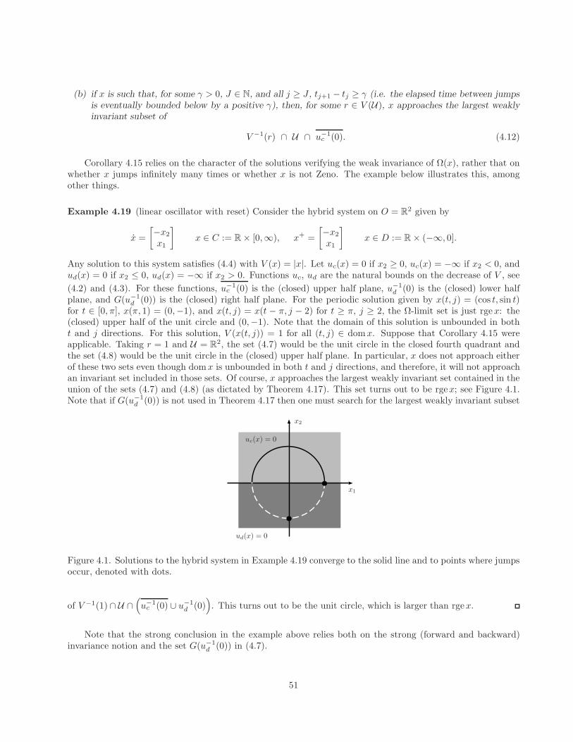
(b) if x is such that, for some γ > 0, J ∈ N, and all j ≥ J , tj+1 − tj ≥ γ (i.e. the elapsed time between jumpsis eventually bounded below by a positive γ), then, for some r ∈ V (U), x approaches the largest weaklyinvariant subset of

V −1(r) ∩ U ∩ u−1c (0). (4.12)

Corollary 4.15 relies on the character of the solutions verifying the weak invariance of Ω(x), rather that onwhether x jumps infinitely many times or whether x is not Zeno. The example below illustrates this, amongother things.

Example 4.19 (linear oscillator with reset) Consider the hybrid system on O = R2 given by

x =

[−x2

x1

]x ∈ C := R × [0,∞), x+ =

[−x2

x1

]x ∈ D := R × (−∞, 0].

Any solution to this system satisfies (4.4) with V (x) = |x|. Let uc(x) = 0 if x2 ≥ 0, uc(x) = −∞ if x2 < 0, andud(x) = 0 if x2 ≤ 0, ud(x) = −∞ if x2 > 0. Functions uc, ud are the natural bounds on the decrease of V , see

(4.2) and (4.3). For these functions, u−1c (0) is the (closed) upper half plane, u−1

d (0) is the (closed) lower halfplane, and G(u−1

d (0)) is the (closed) right half plane. For the periodic solution given by x(t, j) = (cos t, sin t)for t ∈ [0, π], x(π, 1) = (0,−1), and x(t, j) = x(t − π, j − 2) for t ≥ π, j ≥ 2, the Ω-limit set is just rgex: the(closed) upper half of the unit circle and (0,−1). Note that the domain of this solution is unbounded in botht and j directions. For this solution, V (x(t, j)) = 1 for all (t, j) ∈ domx. Suppose that Corollary 4.15 wereapplicable. Taking r = 1 and U = R

2, the set (4.7) would be the unit circle in the closed fourth quadrant andthe set (4.8) would be the unit circle in the (closed) upper half plane. In particular, x does not approach eitherof these two sets even though domx is unbounded in both t and j directions, and therefore, it will not approachan invariant set included in those sets. Of course, x approaches the largest weakly invariant set contained in theunion of the sets (4.7) and (4.8) (as dictated by Theorem 4.17). This set turns out to be rgex; see Figure 4.1.Note that if G(u−1

d (0)) is not used in Theorem 4.17 then one must search for the largest weakly invariant subset

x1

x2

uc(x) = 0

ud(x) = 0

Figure 4.1. Solutions to the hybrid system in Example 4.19 converge to the solid line and to points where jumpsoccur, denoted with dots.

of V −1(1) ∩ U ∩(u−1

c (0) ∪ u−1d (0)

). This turns out to be the unit circle, which is larger than rgex.

Note that the strong conclusion in the example above relies both on the strong (forward and backward)invariance notion and the set G(u−1

d (0)) in (4.7).

51

Note that when applying Theorem 4.17, as a difference to Theorem 4.14, a condition “for all solutions in aset U” has to be checked. A follow-up question is whether conditions that involve a single solution, or in general,a hybrid trajectory (if no data is associated to it) can be stated to obtain information about its convergence.The following lemma states the conditions that two functions need to satisfy along a single hybrid trajectory inorder to characterize the point(s) to which it converges. The results that follow in this section are also statedfor a single hybrid trajectory.

Below, a function f : R≥0 → R is weakly meagre if limn→∞(inft∈In|f(t)|) = 0 for every family In | n ∈ N

of nonempty and pairwise disjoint closed intervals In in R≥0 with infn∈N µ(In) > 0. Here, µ stands for theLebesgue measure. Moreover, f is weakly meagre if for some τ > 0,

limM→∞

∫ M+τ

M

|f(t)| dt = 0. (4.13)

In particular, any L1 function is weakly meagre.

Lemma 4.20 (meagre-limsup conditions) Let x be a complete hybrid trajectory such that

(*) For each z ∈ Ω(x) and ǫ > 0 there exist δ > 0 and T > 0 such that, if x(t, j) ∈ z + δB for some(t, j) ∈ domx then x(t′, j) ∈ z + ǫB for all t′ ∈ [t− T, t+ T ] such that (t′, j) ∈ domx.

Furthermore, suppose that for some set U ⊂ O with rgex ⊂ U there exist functions ℓc, ℓd : U → [0,∞] that, forthe hybrid trajectory x, satisfy the meagre-limsup conditions given by

(a) if the projection of domx onto R≥0 is unbounded then t 7→ ℓc(x(t, j(t))) is weakly meagre,

(b) if the projection of domx onto N is unbounded then for all large enough j there exists t∗j ∈ [t(j), t(j + 1)]such that lim supj→∞ ℓd(x(t

∗j , j)) = 0.

Then Ω(x) ⊂ Ex,ℓc∪Ex,ℓd

, where Ex,ℓcand Ex,ℓd

are respectively defined by

z ∈ rgex | ∃zi → z, zi ∈ rgex, lim inf i→∞ ℓc(zi) = 0,z ∈ rgex | ∃zi → z, zi ∈ rgex, lim inf i→∞ ℓd(zi) = 0.

Proof. Suppose otherwise, that for some x∗ ∈ Ω(x) and ǫ, γ > 0,

ℓ(z) := minℓc(z), ℓd(z) ≥ γ

for all z ∈ x∗ + ǫB, z ∈ rgex. By definition of ω-limit point, there is an increasing and unbounded sequence(ti, ji) ∈ domx with x(ti, ji) → x∗ as i→ ∞. We can assume that for all i, ti + ji +1 ≤ ti+1 + ji+1. Let δ, T > 0be related to x∗, ǫ as in condition (*) and, without loss of generality, suppose that T < 1. Ignoring initial termsif necessary, we have x(ti, ji) ∈ x∗ + δB for all i ∈ N. Consequently, x(t, ji) ∈ x∗ + δB for all t ∈ [ti − T, ti + T ],(t, ji) ∈ domx. For each i, either of the two conditions holds:

(1’) either t(ji) ≤ ti − T or t(ji + 1) ≥ ti + T (x flows for time T either before ti or after ti)

(2’) t(ji) > ti − T and t(ji + 1) < ti + T (x jumps within time T before and after ti)

Either (1’) or (2’) has to occur for infinitely many i’s. Suppose it is (1’) and that t(ji) ≤ ti − T for suchi’s (the other case is treated similarly). Then, domx must be unbounded in the t-direction. The fact thatℓ(x(t, j(t))) > γ for any t ∈ [ti − T, ti] for infinitely many i’s contradicts weak meagreness of t 7→ ℓc(x(t, j(t)))

52

(note that intervals [ti −T, ti] are disjoint). If (2’) holds for infinitely many i’s, then domx is unbounded in thej-direction, and for infinitely many i’s and all t ∈ [t(ji), t(ji + 1)] we have ℓd(x(t, ji)) > γ. This contradicts (b).

The condition (*) above can be viewed as a sort of continuity of x(t, j) in t, uniform “near each point ofΩ(x)”. The condition automatically holds if x is a solution to a hybrid system that satisfies (S1) and (S2) andthe hybrid basic conditions. In fact, since F is locally bounded, x(t, j) is Lipschitz in t, locally “near each pointof Ω(x)”.

In Lemma 4.20, Ex,ℓc⊂ z ∈ rgex | ℓc(z) = 0, where ℓc is the lower semicontinuous closure of ℓc.

(Given a set U and a function ℓ : U → [−∞,∞], its lower semicontinuous closure ℓ : U → [−∞,∞], is thegreatest lower semicontinuous function defined on U , bounded above by ℓ on U . Equivalently, for any x ∈ U ,ℓ(x) = lim infxi→x ℓ(xi). In this terminology, Ex,ℓ is the zero-level set of the lower semicontinuous closure of thefunction ℓ truncated to rgex.) In particular, if both ℓc and ℓd are lower semicontinuous, and rgex ⊂ U , thenthe conclusion of Lemma 4.20 implies that Ω(x) is a subset of

z ∈ rgex | ℓc(z) = 0 ∪ z ∈ rgex | ℓd(z) = 0.

However, if the assumption that ℓc, ℓd are nonnegative was weakened to say that they are nonnegative only onrgex, the last conclusion above may fail.

The following result corresponds to an invariance principle involving the meagre-limsup conditions whichautomatically follows from Lemma 4.20.

Theorem 4.21 (meagre-limsup invariance principle) Let x be a precompact hybrid trajectory. Suppose thatfor U ⊂ O, rgex ⊂ U , there exist functions ℓc, ℓd : U → [0,∞] for which the meagre-limsup conditions hold.Then x converges to the largest weakly invariant subset of

z ∈ U | ℓc(z) = 0 ∪ z ∈ U | ℓd(z) = 0.

If rgex ⊂ U and ℓc, ℓd are lower semicontinuous, then all the closure operations above can be removed.

Let x be a precompact hybrid trajectory for which there exist functions uc, ud : O → [−∞, 0] and V : O → R

such that (4.4) holds for the hybrid trajectory x for all (t, j), (t′, j′) ∈ domx such that (t, j) (t′, j′). Thenℓc = −uc, ℓd = −ud satisfy conditions (a) and (b) of Theorem 4.20. In fact, there exists a constant M > 0 forwhich ∫ T

0

ℓc(x(t, j(t))) dt < M,

J∑

j=0

ℓd(x(t(j + 1), j)) < M,

for any (T, J) ∈ domx (this shows that ℓc(t, j(t)) is integrable on [0,∞) and thus weakly meagre, while tosatisfy (b), one can take t∗j = t(j + 1).

Based on the previous discussion, the next result shows that, when a function V with the right propertiesexists, the conditions (a) and (b) of Lemma 4.20 are guaranteed.

Corollary 4.22 (meagre-limsup conditions with a V ) Let x be a precompact hybrid trajectory. Suppose thatthere exists a continuous function V : O → R, and functions uc, ud : O → [−∞,∞] such that for some(T, J) ∈ domx,

uc(x(t, j)) ≤ 0, ud(x(t, j)) ≤ 0

for all (t, j) ∈ domx with (T, J) (t, j), and (4.4) holds for the hybrid trajectory x for all (t, j), (t′, j′) ∈ domxsuch that (T, J) (t, j) (t′, j′). Then Ω(x) ⊂ Ex,uc ∪ Ex,ud , where Ex,uc and Ex,ud are respectively definedby

53

z ∈ rgex | ∃zi → z, zi ∈ rgex, lim supi→∞ uc(zi) = 0,z ∈ rgex | ∃zi → z, zi ∈ rgex, lim supi→∞ ud(zi) = 0.

More precise results can be obtained if the hybrid time domain of the hybrid trajectory is bounded in eitherthe t or j direction.

Corollary 4.23 (special cases for meagre-limsup conditions) Let x be a complete hybrid trajectory for which(*) holds.

(a) If the projection of domx onto N is bounded and there exists a function ℓc : rgex → [0,∞] such thatt 7→ ℓc(x(t, j(t))) is weakly meagre, then Ω(x) ⊂ Ex,ℓc

.

(b) If the projection of domx onto R≥0 is bounded and there exists a function ℓd : rgex→ [0,∞] such that, forall large enough j, there exists t∗j ∈ [t(j), t(j+1)] such that lim supj→∞ ℓd(x(t

∗j , j)) = 0, then Ω(x) ⊂ Ex,ℓd

.

If, for a hybrid trajectory, the elapsed time between jumps is uniformly positive then only (a) of themeagre-limsup conditions needs to be checked to draw the conclusion of Lemma 4.20.

Corollary 4.24 (meagre-limsup invariance with uniformly bounded time between jumps) Let x be a completehybrid trajectory such that (*) holds and tj+1 − tj ≥ γ > 0 for all j = 1, 2, . . .. If there exists a functionℓc : rgex→ [0,∞] such that condition (a) of the meagre-limsup conditions holds, then Ω(x) ⊂ Ex,ℓc

.

Proof. In the proof of Lemma 4.20, T can be chosen arbitrarily small. Picking T < γ2 shows that (2’) in the

proof of Lemma 4.20 cannot hold; hence (1’) has to hold for infinitely many times. The proof follows that ofLemma 4.20.

If multiple instantaneous jumps can occur “only on the zero level set of ℓd” (for a hybrid system H, thisis equivalent to ℓd (G(D) ∩D) = 0) and x is precompact, then only (a) of the meagre-limsup conditions needsto be checked to draw the conclusion of Lemma 4.20. This is because under such an assumption on the jumps,on each compact set away from the zero level set of ℓd, the elapsed time between jumps is uniformly boundedbelow by a positive constant.

Corollary 4.25 (case of multiple instantaneous jumps) Given the function ℓd : O 7→ R≥0, assume that for allx ∈ SH, if (t, j−1), (t, j), (t, j+1) ∈ dom x, then ℓd(x(t, j)) = 0. Let x ∈ SH be a precompact solution. Supposethat there exists a function ℓc : rgex → [0,∞] such that condition (a) of the meagre-limsup conditions holds.Then the conclusion of Lemma 4.20 is true.

4.2.4 Connections to observability and detectability

Classically, (zero-state) observability means that if the output of a system is held to zero, the state is identicallyzero. The following definition extends this concept to hybrid systems.

Definition 4.26 (observability) Given sets A,K ⊂ O, the distance to A is observable relative to K for thehybrid system H if for every nontrivial solution x satisfying rgex ⊂ K then |x(t, j)|A = 0 for all (t, j) ∈ domx.

If, for a certain (output) function h : O → Rk, K = h−1(0), then it is said that the distance to A is

observable through (the output) h.

Basic properties based on observability are stated below, under the assumption that A and K are compactsubsets of O and the distance to A is observable relative to K.

54

Theorem 4.27 (observability and the invariance principle) Let A,K ⊂ O be compact, and suppose that A isstable relative to K for the hybrid system H. Then the following statements are equivalent:

1. The distance to A is observable relative to K.

2. The largest weakly invariant set in K is a subset of A.

In differential equations, detectability is the property that when the output is held to zero, complete solutionsx satisfy limt→∞ |x(t)|A = 0. Below, this notion is generalized.

Definition 4.28 (detectability) Given sets A,K ⊂ O, the distance to A is detectable relative to K for H if forevery complete solution x ∈ SH satisfying rgex ⊂ K then lim inft+j→∞ |x(t, j)|A = 0.

This detectability notion above can be understood as x having an ω-limit point at A. As for observabilityrelative to K := h−1(0) for some function h : O → R

k, it is said that the distance to A is detectable through h.

When detectability (as in Definition 4.28) is combined with relative stability, the usual detectability isrecovered.

Lemma 4.29 (detectability and relative stability) Let A,K ⊂ O be compact. If the distance to A is detectablerelative to K and A is stable relative to K, then each complete solution x ∈ x with rgex ⊂ K converges to A.

Example 4.30 (hybrid system with linear dynamics) For x ∈ Rn, A1, A2 ∈ R

n×n, and closed C,D ⊂ Rn,

consider the hybrid system H given by

x = A1x when x ∈ C, x+ = A2x when x ∈ D.

For simplicity, assume that C∪D = Rn. The motivation for this type of systems comes from many applications,

like sample-data control, reset systems, etc. Suppose that:

() Let C ∈ Rm×n be such that there exists matrices L1, L2, and P = PT > 0 that satisfy

xT

((A1 + L1C

)T

P + PT(A1 + L1C

))x < 0,

xT

((A2 + L2C

)T

P(A2 + L2C

)− P

)x < 0,

where the first inequality is for all x ∈ C \ 0 and the second one for all x ∈ D \ 0.

This assumption holds in particular when the pairs (C, A1) and (C, A2) are detectable (in the linear sense) andthe detectability of both pairs can be verified with a common Lyapunov function (which is quadratic and givenby P ).

Let K be any subset ofz ∈ R

n∣∣∣ Cz = 0

and A = 0 ⊂ R

n. By definition of K, solutions that remain

in K are also solutions of the output injected hybrid system HO defined as

x = (A1 + L1C)x x ∈ C, x+ = (A2 + L2C)x x ∈ D.

Stability of A (for the system above, and hence for H relative to K) can be easily verified with the use of thecommon quadratic Lyapunov function V (x) = xTPx. Moreover, by Corollary 4.14 with U = R

n and V (x),

55

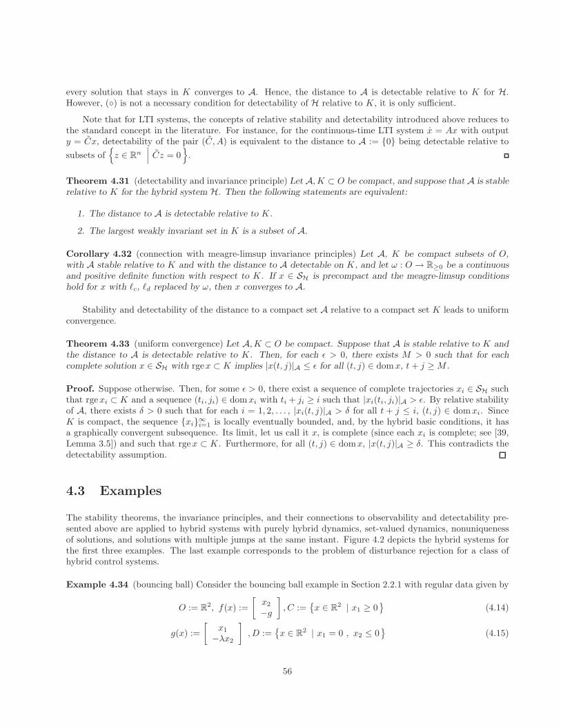
every solution that stays in K converges to A. Hence, the distance to A is detectable relative to K for H.However, () is not a necessary condition for detectability of H relative to K, it is only sufficient.

Note that for LTI systems, the concepts of relative stability and detectability introduced above reduces tothe standard concept in the literature. For instance, for the continuous-time LTI system x = Ax with outputy = Cx, detectability of the pair (C, A) is equivalent to the distance to A := 0 being detectable relative to

subsets ofz ∈ R

n∣∣∣ Cz = 0

.

Theorem 4.31 (detectability and invariance principle) Let A,K ⊂ O be compact, and suppose that A is stablerelative to K for the hybrid system H. Then the following statements are equivalent:

1. The distance to A is detectable relative to K.

2. The largest weakly invariant set in K is a subset of A.

Corollary 4.32 (connection with meagre-limsup invariance principles) Let A, K be compact subsets of O,with A stable relative to K and with the distance to A detectable on K, and let ω : O → R≥0 be a continuousand positive definite function with respect to K. If x ∈ SH is precompact and the meagre-limsup conditionshold for x with ℓc, ℓd replaced by ω, then x converges to A.

Stability and detectability of the distance to a compact set A relative to a compact set K leads to uniformconvergence.

Theorem 4.33 (uniform convergence) Let A,K ⊂ O be compact. Suppose that A is stable relative to K andthe distance to A is detectable relative to K. Then, for each ǫ > 0, there exists M > 0 such that for eachcomplete solution x ∈ SH with rgex ⊂ K implies |x(t, j)|A ≤ ǫ for all (t, j) ∈ domx, t+ j ≥M .

Proof. Suppose otherwise. Then, for some ǫ > 0, there exist a sequence of complete trajectories xi ∈ SH suchthat rgexi ⊂ K and a sequence (ti, ji) ∈ domxi with ti + ji ≥ i such that |xi(ti, ji)|A > ǫ. By relative stabilityof A, there exists δ > 0 such that for each i = 1, 2, . . . , |xi(t, j)|A > δ for all t + j ≤ i, (t, j) ∈ domxi. SinceK is compact, the sequence xi∞i=1 is locally eventually bounded, and, by the hybrid basic conditions, it hasa graphically convergent subsequence. Its limit, let us call it x, is complete (since each xi is complete; see [39,Lemma 3.5]) and such that rgex ⊂ K. Furthermore, for all (t, j) ∈ domx, |x(t, j)|A ≥ δ. This contradicts thedetectability assumption.

4.3 Examples

The stability theorems, the invariance principles, and their connections to observability and detectability pre-sented above are applied to hybrid systems with purely hybrid dynamics, set-valued dynamics, nonuniquenessof solutions, and solutions with multiple jumps at the same instant. Figure 4.2 depicts the hybrid systems forthe first three examples. The last example corresponds to the problem of disturbance rejection for a class ofhybrid control systems.

Example 4.34 (bouncing ball) Consider the bouncing ball example in Section 2.2.1 with regular data given by

O := R2, f(x) :=

[x2

−g

], C :=

x ∈ R

2 | x1 ≥ 0

(4.14)

g(x) :=

[x1

−λx2

], D :=

x ∈ R

2 | x1 = 0 , x2 ≤ 0

(4.15)

56

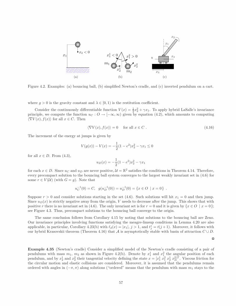
(a) (b)

x1

x2

x3

x4u

(c)

Figure 4.2. Examples: (a) bouncing ball, (b) simplified Newton’s cradle, and (c) inverted pendulum on a cart.

where g > 0 is the gravity constant and λ ∈ [0, 1) is the restitution coefficient.

Consider the continuously differentiable function V (x) = 12x

22 + γx1. To apply hybrid LaSalle’s invariance

principle, we compute the function uC : O → [−∞,∞) given by equation (4.2), which amounts to computing〈∇V (x), f(x)〉 for all x ∈ C. Then

〈∇V (x), f(x)〉 = 0 for all x ∈ C . (4.16)

The increment of the energy at jumps is given by

V (g(x)) − V (x) = −1

2(1 − e2)x2

2 − γx1 ≤ 0

for all x ∈ D. From (4.3),

uD(x) = −1

2(1 − e2)x2

2 − γx1

for each x ∈ D. Since uC and uD are never positive, U = R2 satisfies the conditions in Theorem 4.14. Therefore,

every precompact solution to the bouncing ball system converges to the largest weakly invariant set in (4.6) forsome r ∈ V (U) (with G = g). Note that

u−1C (0) = C, g(u−1

D (0)) = u−1D (0) = x ∈ O | x = 0 .

Suppose r > 0 and consider solutions starting in the set (4.6). Such solutions will hit x1 = 0 and then jump.Since uD(x) is strictly negative away from the origin, V needs to decrease after the jump. This shows that withpositive r there is no invariant set in (4.6). The only invariant set is for r = 0 and it is given by x ∈ O | x = 0;see Figure 4.3. Thus, precompact solutions to the bouncing ball converge to the origin.

The same conclusion follows from Corollary 4.15 by noting that solutions to the bouncing ball are Zeno.Our invariance principles involving functions satisfying the meagre-limsup conditions in Lemma 4.20 are alsoapplicable, in particular, Corollary 4.23(b) with ℓd(x) = |x1|, j > 1, and t∗j = t(j+1). Moreover, it follows withour hybrid Krasovskii theorem (Theorem 4.16) that A is asymptotically stable with basin of attraction C ∪D.

Example 4.35 (Newton’s cradle) Consider a simplified model of the Newton’s cradle consisting of a pair ofpendulums with mass m1, m2 as shown in Figure 4.2(b). Denote by x1

1 and x21 the angular position of each

pendulum, and by x12 and x2

2 their tangential velocity defining the state x = [x11 x

21 x

12 x

22]

T . Viscous friction forthe circular motion and elastic collisions are considered. Moreover, it is assumed that the pendulums remainordered with angles in (−π, π) along solutions (“ordered” means that the pendulum with mass m1 stays to the

57

x1

x2

ξV −1(r)

C

D

Figure 4.3. A solution to the bouncing ball system in the x1 − x2 plane and a level set of V (dashed). Solutionsescape a level set with r > 0 in finite time.

left of the pendulum with mass m2 along solutions). More general models allowing the pendulums to changetheir order can be derived but for simplicity, they are not pursued here. Let O = (−π, π) × (−π, π) × R

2.

The equations of motion for the pendulums in between collisions are given by Newton’s laws

xi1 = xi

2, xi2 = −γ

lsin(xi

1) − bixi2 , (4.17)

when either x11 ≤ x2

1 (pendulums in the right order) or x12 ≤ x2

2 (pendulums moving in the right direction),where i = 1, 2, bi > 0, γ > 0 is the gravity constant, and l > 0 is the length of the pendulums. Jumps areassumed to happen when x1

1 ≥ x21 and x1

2 ≥ x22. When this holds, the state is updated by

x+1 =

[11

]arg min

s∈x11,x2

11 − cos(s) , x+

2 = Mx2 , (4.18)

where x1 = [x11 x

21]

T , x2 = [x12 x

22]

T , and the matrix M characterizes the exchange of kinetic energy at impacts.Note that the angular positions are mapped to the minimal potential energy configuration (typically, collisionsbetween the pendulums occur when x1

1 = x21). When the usual impact rule with conservation of momentum is

used, the jump mapping for velocities is

(x12)

+ − (x22)

+ = −e(x1

2 − x22

),

m1(x12)

+ +m2(x22)

+ = m1x12 +m2x

22 ,

where e ∈ [0, 1] is the restitution coefficient. In this case

M =

[λ− (1 − λ)e (1 − λ)(1 + e)λ(1 + e) 1 − λ− λe

], (4.19)

where λ = m1

m1+m2∈ (0, 1). For the following analysis, it is assumed that M is given as in (4.19).

The continuous dynamics of the Newton’s cradle system are given by f(x) which is the vector functionresulting from stacking the vector fields given in (4.17) for i = 1, 2. The flow and jump sets are given by

C :=x ∈ O

∣∣ x11 ≤ x2

1 or x12 ≤ x2

2

, D :=

x ∈ O

∣∣ x11 ≥ x2

1, x12 ≥ x2

2

.

The jump mapping on D is given by g(x), the vector function constructed by stacking the mappings in (4.18).

58

Let J =

[λ 00 1 − λ

]. It is easy to show that MTJM − J ≤ 0. Moreover, the data of the Newton’s cradle

system satisfies the hybrid basic conditions.

Let V be the energy of the system normalized by m1 +m2:

V (x) =1

2l2xT

2 J x2 + γλl(1 − cos(x1

1))

+ γ(1 − λ)l(1 − cos(x2

1)). (4.20)

It turns out that for all x ∈ C

〈∇V (x), f(x)〉 = −λb1l2(x1

2

)2 − (1 − λ)b2l2(x2

2

)2 ≤ 0 .

Thus, with (4.2), uC(x) = −λb1l2(x1

2

)2 − (1− λ)b2l2(x2

2

)2for all x ∈ C. At jumps, V (g(x))− V (x) is given by

l2

2xT

2

(MTJM − J

)x2 + γl(1 − cos(s∗)) − γλl

(1 − cos(x1

1))− γ(1 − λ)l

(1 − cos(x2

1)),

where s∗ = arg mins∈x11,x2

11 − cos(s). It follows that V (g(x)) − V (x) ≤ 0, and for each point in D, defines

uD.

To apply hybrid LaSalle’s invariance principle, compute

u−1C (0) =

x ∈ O

∣∣ x12 = x2

2 = 0,

u−1D (0) =

x ∈ O

∣∣ x11 = x2

1, xT2 (MTJM − J )x2 = 0

.

The set u−1C (0) follows from the definition of C and uC above. To find u−1

D (0) note that points x ∈ D withx1

1 = x21 are such that s∗ = x1

1 = x21, and consequently, uD is zero only if xT

2 (MTJM−J )x2 = 0. The remainingpoints in D are such that x1

1 6= x21. Since the first term of uD is nonpositive and the remaining terms are strictly

negative for x11 6= x2

1, points with x11 6= x2

1 are not in u−1D (0). When g acts on u−1

D (0), the angles are mapped totheir same value and the velocities are mapped to (x1

2)+, (x2

2)+ with (x1

2)+ ≤ (x2

2)+. Using the jump rule (4.18)

and the properties of M and J

u−1D (0) ∩ g(u−1

D (0)) =x ∈ O

∣∣ x11 = x2

1, x12 = x2

2

.

By Theorem 4.14 with U = O, every precompact solution converges to the largest weakly invariant set in(4.6) for some r ∈ V (U) (with G = g). Solutions starting in u−1

C (0) and staying in the largest weakly invariantsubset of (4.6) need to have same angles. Therefore, only points with x1

1 = x21 in u−1

C (0) qualify for the invarianceproperty. It follows that

u−1C (0) ∪

(u−1

D (0) ∩ g(u−1D (0))

)=

x ∈ O

∣∣ x11 = x2

1, x12 = x2

2

.

For every ξ in this set, there exists one discrete solution that stays in it. Then, precompact solutions approach

V −1(r) ∩x ∈ O

∣∣ x11 = x2

1, x12 = x2

2

for some r = V (U). Note that the same conclusion holds when the jump map for the angles is the identity andthe inequality condition for the angles in D is replaced by equality.

The invariance principle shows that solutions to the Newton’s cradle system approach points with equalangles and velocities. The reason for this is that with the jump map considered above, the kinetic energy of theballs remains constant when the pendulums collide with equal velocity. This generates solutions that after sucha collision, jump for all time (discrete solutions). This undesirable behavior can be removed by including the“spring effect” at collisions (or when the balls are touching). (Another option is to redefine the collision rule,

59

this is not pursue this here.) To model the “spring effect” we add temporal regularization by means of a timerτ with continuous dynamics τ = 1 − τ , jump map τ+ = 0, and temporal regularization constant δ ∈ (0, 1).

The hybrid system for the model of the Newton’s cradle with temporal regularization has state x =[x1

1 x21 x

12 x

22 τ ]

T and state space given by Oτ = R5. The flow and jump sets under temporal regularization are

given byCτ :=

x ∈ Oτ

∣∣ x11 ≤ x2

1 or x12 ≤ x2

2 or τ ∈ [0, δ],

Dτ :=x ∈ Oτ

∣∣ x11 ≥ x2

1, x12 ≥ x2

2, τ ≥ δ.

The continuous dynamics are given by f τ (x) which is the vector function resulting from stacking the vectorfield f(x) and the timer dynamics defined above. The jump mapping is given by gτ (x), the vector functionconstructed by stacking the mapping g(x) and the jump mapping for the timer.

For the energy function given by equation (4.20), the functions uC and uD, and their zero-level sets turnout to be the same as above but with the addition of the timer state τ .

By Theorem 4.14 with U = Oτ , every precompact solution converges to the largest weakly invariant set in(4.6) for some r ∈ V (U) (with G = gτ ). Note that in this case, u−1

D (0) ∩ gτ (u−1D (0)) = ∅. Then by Lemma 4.9

and Corollary 4.15(b) with U = Oτ , precompact solutions converge to the largest weakly invariant subset in

V −1(r) ∩ U ∩ u−1C (0) = V −1(r) ∩

x ∈ Oτ

∣∣ x12 = x2

2 = 0

for some r ∈ V (U). From the continuous dynamics of the system, that largest weakly invariant subset is givenfor r = 0 and is equal to

A :=x ∈ O

∣∣ xi1 = xi

2 = 0, i = 1, 2, τ ∈ [0, δ].

Hence, precompact solutions that stay in U are such that the pendulums converge to the resting position. Localasymptotic stability of A follows from Theorem 4.16.

Example 4.36 (pendulum swing-up with hybrid control) Consider an inverted pendulum on a cart controlledby an external input force u as shown in Figure 4.2(c). The variable x1 is the pendulum angle (x1 = 0 is thevertical upright position), x2 is the angular velocity, x3 is the cart position, and x4 is the cart velocity. Aftera preliminary input feedback transformation of the form u = ψ(x) + φ(x)u, a hybrid model of the resultingsystem can be written as

x = f(x, u) x ∈ Cπ , x+ = g(x) x ∈ Dπ,

where

f(x, u) := [x2γ

lsin(x1) −

1

lcos(x1)u x4 u]T ,

g(x) := [(x1 − 2πZ) ∩ [−π, π] x2 x3 x4]T ,

Cπ :=x ∈ R

4 | |x1| ≤ π + µ,

Dπ =x ∈ R

4 | |x1| ≥ π + µ.

where µ is a positive constant, γ > 0 is the gravity constant, and l > 0 the length of the pendulum. The purposeof the jump mapping g is to keep the angle x1 bounded (g remaps x1 to the set [−π, π] at every jump.)

The proposed hybrid swing-up strategy chooses the appropriate feedback control law depending on thelocation of the pendulum. When the pendulum is in the region i, the control law is given by k(·, i), i ∈ Q :=1, 2, 3. Let W (x) be the energy of the pendulum and c1, c2 be constants that are sufficiently close to butlarger than minx∈R4 W (x) and satisfy c1 > c2. Take U3a and U3b, U3a ⊂ U3b, to be closed neighborhoods of theorigin in R

2 contained in [−π, π] × R, such that for the system x = f(x, u), the control law k(·, 3) renders the

60

origin (in R4) locally asymptotically stable with basin of attraction containing U3b ×R

2 and such that solutionsstarting in U3a × R

2 do not reach the boundary of U3b × R2.

Define three regions by the sets Ωi and Ci (Ωi ⊂ Ci), i ∈ Q, as follows

Ω1 = C1 =x ∈ R

4 | W (x) ≤ c1

Ω3 = U3a × R2, C3 = U3b × R

2

Ω2 =x ∈ R2 \ U3a × R

2 | W (x) ≥ c1

C2 =x ∈ R2 \ U3a × R

2 | W (x) ≥ c2

As previously stated, the control law in the set C3 is given by k(·, 3). In the region defined by C2, the controlk(·, 2) is designed to inject enough energy into the system so that U3a is reached. The control law for the setC1 is given by k(·, 1) which is designed to drive the system away from the resting condition (e.g. k(x, 1) = 1).

The state of the closed-loop system is denoted by (x, q) where x ∈ R4 and q ∈ Q. Define the state

space O := R5. For each i ∈ Q, Di := R4 \ Ci ∩ Cπ, D :=

(x, q) ∈ R

4 ×Q | x ∈ Dq

∪ Dπ, C :=

(x, q) ∈ R4 ×Q | x ∈ Cq ∩ Cπ

, and Ψ(q) := ∪p<q,p∈QΩp. The closed-loop system defines a hybrid system HI

that can be written asx = f(x, k(x, q)), q = 0 (x, q) ∈ C,

[xq

]+

= G(x, q) (x, q) ∈ D,

where G(x, q) is defined by

[g(x)q

]x ∈ Dπ \Dq

G1(x, q) x ∈ (Dq ∩ Ψ(q)) \Dπ

G2(x, q) x ∈ Dq \ (Ψ(q) ∪Dπ)[g(x)q

], G1(x, q)

x ∈ Dq ∩ Ψ(q) ∩Dπ

[g(x)q

], G2(x, q)

x ∈ (Dq \ Ψ(q)) ∩Dπ,

where

G1(x, q) :=

[x

p ∈ Q | x ∈ Ωp

],

G2(x, q) :=

[x

p ∈ Q | p > q, x ∈ Ωp

].

Note that the hybrid system HI satisfies (A0)-(A3). Note that there exists initial conditions for whichsolutions are nonunique. For instance, there exist (ξ, 1) ∈ (Ω1 ∩ Ω2) ×Q such that either q immediately jumpsto 2 and then flows according to x = f(x, k(x, 2)) or else flows according to x = f(x, k(x, 1)) while remainingin Ω1 until flows are not longer possible and then q jumps to 2.

To show that solutions converge to the compact set A := 0 × 3 ⊂ O. Consider the continuouslydifferentiable function V (x, q) = 1/q. Since the continuous dynamics of q are such that q(t, j) remains constantduring flows, V does not increase along flows and uC is identically zero. The design of the controller guaranteesthat solutions starting with initial x and q in Ω1 ×1 will sequentially transition from region 1 to region 2 and

61

finally to region 3. Solutions starting with arbitrary initial conditions will be mapped after the first jump toU := ∪3

i=1Ωi × i and from there on will follow the transition rule. Then

uD(x, q) =1

η− 1

q< 0

where η ∈ Q, η > q, (x, q) ∈ U . By Theorem 4.14, precompact solutions that stay in U approach the largestweakly invariant set in (4.6) for some r ∈ V (U). From the previous definitions, u−1

C (0) = C, u−1D (0) = ∅. Then

the set (4.6) is given by V −1(r) ∩ U ∩ C. By construction of the controller, the largest weakly invariant setcontained in this set is for r = 1

3 and is equal to A. Thus, by Theorem 4.14, precompact solutions to HI

converge to A, i.e. pendulum in the straight-up position and zero position and velocity of the cart.

The same result can be obtained by means of detectability. Let K = C3 × 3. Every solution (x, q)satisfying rge(x, q) ⊂ K has q(t, j) = 3 for all (t, j) ∈ dom(x, q). Since the control law in C3 is the localstabilizer for the origin (in R

4), the compact set A is stable relative to K and the distance to A is detectablerelative to K for HI . Given a precompact solution (x, q) to HI , let K ′ = K ∩ rge(x, q). Detectability andstability of A relative to K ′ automatically holds since K ′ ⊂ K. Then, by Corollary 4.32, with ω being thedistance to K, precompact solutions x to HI converge to A. Note that the meagre-limsup conditions hold forω since, by design of the controller, for each solution (x, q) there exists T ∗ such that (x(t, j), q(t, j)) ∈ K ′ for allt+ j ≥ T ∗, (t, j) ∈ dom(x, q).

Example 4.37 (disturbance rejection) Consider the control of a nonlinear system x = f(x, u, d) with state x,control input u, and disturbance input d, by a hybrid controller Hc with state xc. Let the closed-loop hybridsystem Hcl be

ξ = fcl(ξ, d) ξ ∈ Ccl, ξ+ = gcl(ξ) ξ ∈ Dcl ,

with output y = hcl(ξ), where ξ := [x, xc]T ∈ R

nc , fcl : Rnc ×R

m → Rnc , gcl : R

nc → Rnc , and hcl : R

nc → Rmc

are continuous. Suppose that the following holds for Hcl.

Assumption 4.38 (Hcl conditions 1)

1. There exists a continuously differentiable, positive definite, radially unbounded function Vcl : Rnc → R≥0

and γcl ≥ 0 such that〈∇Vcl(ξ), fcl(ξ, ucl)〉 ≤ −|hcl(ξ)|2 + γ2

cl|ucl|2

∀ξ ∈ Ccl, ucl ∈ Rm; and Vcl(gcl(ξ)) ≤ Vcl(ξ) ∀ξ ∈ Dcl.

2. The hybrid closed-loop system Hcl with d ≡ 0 is such that the distance of the state ξ to the origin (inR

nc) is detectable relative to the set Kcl := ξ ∈ Rnc | hcl(ξ) = 0.

Let xd = fd(xd, ud) with output yd = hd(xd) be the model for the disturbance d where xd ∈ Rn; fd : R

n×Rmc →

Rn, hd : R

n → Rm are continuous. Below, ‖ · ‖2 denotes the L2-norm and ‖ · ‖∞ denotes the L∞-norm.

Assumption 4.39 (disturbance model conditions) The disturbance model satisfies

1. There exist γd ≥ 0 and ρd ∈ K∞ s.t. ‖yd‖2 ≤ γd‖ud‖2 +ρd(|xd(0)|), ‖xd‖∞ ≤ ρd (‖yd‖2 + ‖ud‖2 + |xd(0)|)∀ud ∈ L2, xd(0) ∈ R

n.

2. When ud ≡ 0, the distance of the state xd to the origin (in Rn) is detectable relative to the set Kd :=

xd ∈ Rn | hd(xd) = 0.

Under the following additional assumptions:

62

Assumption 4.40 (Hcl conditions 2) Ccl, Dcl are relatively closed in Rnc , Ccl∪Dcl = R

nc , and gcl(Dcl)∩Dcl =∅;

Assumption 4.41 (gain condition) γdγcl < 1;

the origin of the closed-loop system, denoted by H, resulting of interconnecting Hcl with the disturbance modelis globally asymptotically stable.

To show the claim, let ζ = [ξT , xTd ]T be a maximal solution to H and let E := dom ζ ∩ ([0, T ]× 0, . . . , J)

be a compact subset of dom ζ (Recall that it is possible to write E = ∪Ji=0[ti, ti+1] × i where t0 = 0 and

tJ+1 = T .) By Assumption 4.38.1, it follows that

∫ T

0

|hcl(ξ(t, j(t)))|2dt ≤ γ2cl

∫ T

0

|hd(xd(t, j(t)))|2dt+J∑

i=0

[−Vcl(ξ(ti+1, j(ti))) + Vcl(ξ(ti, j(ti)))] .

Note that by Assumption 4.40 and Lemma 4.9, for every 0 ≤ i ≤ J , the intervals [ti, ti+1] ⊂ [0, T ] have non-zerolength, and therefore, contribute to the integrals above. Using Assumption 4.38.1 and positive definiteness ofVcl

(‖hcl(ξ)‖S

2

)2 ≤ Vcl(ξ(0, 0)) + γ2cl

(‖hd(xd)‖S

2

)2,

where ‖hd(xd)‖S2 denotes

√∫ T

0|hd(xd(t, j(t)))|2dt.

Let ud(t) = hcl(ξ(t, j(t))) for all t ∈ [0, T ], ud(t) = 0 for all t > T . For each t ∈ [0, T ], ud generatesyd(t) = hd(xd(t, j(t))). Then, using ud, yd in Assumption 4.39.1, the bound on the norm of hcl(ξ) and hd(xd)are

‖hcl(ξ)‖S2 ≤ 1

1 − γdγcl

(√Vcl(ξ(0, 0)) + γclρd(|xd(0, 0)|)

),

‖hd(xd)‖S2 ≤ 1

1 − γdγcl

(γd

√Vcl(ξ(0, 0)) + ρd(|xd(0, 0)|)

).

By Assumption 4.41, 11−γdγcl

∈ (0,∞). Integrating the flow condition in Assumption 4.38.1 along ξ(t, j) from 0

to some t, (t, j(t)) ∈ dom ζ, (t, j(t)) (T, J), yields

∫ t

0

d

dτVcl(ξ(τ, j(τ)))dτ ≤ γ2

cl

(‖hd(xd)‖S

2

)2.

Using the nonincreasing condition at jumps gives

Vcl(ξ(t, j(t))) ≤ γ2cl

(‖hd(xd)‖S

2

)2+ Vcl(ξ(0, 0)).

Since Vcl is radially unbounded, there exists α ∈ K∞ that satisfies α(|z|) ≤ Vcl(z) for all z ∈ Rnc . It follows

that

‖ξ‖S∞ ≤ α−1

(Vcl(ξ

0) + γ1

(γd

√Vcl(ξ0) + ρd(|x0

d|))2

)

‖xd‖S∞ ≤ ρd

(γ2

√Vcl(ξ0) + γ3ρd(|x0

d|) + |x0d|

)

where ‖ξ‖S∞ means sup(t,j)∈S |ξ(t, j)|, γ1 :=

γ2cl

(1−γdγcl)2, γ2 := 1+γd

1−γdγcl, γ3 := 1+γcl

1−γdγcl, ξ0 = ξ(0, 0), and x0

d =

xd(0, 0). Note that the bounds for the norm of the states ξ, xd and the outputs hcl(ξ), hd(xd) are independentof the compact hybrid time domain S. Therefore those bounds can be extended to the entire domain dom ζ.

63

Since ζ is maximal and bounded, and since Ccl ∪Dcl = Rnc , by Proposition 2.1 in [39], ζ must be complete,

i.e. ζ is precompact. Thus, the origin (in Rnc × R

n) is stable.

Let ℓ(ζ) = |hcl(ξ)|2 + |hd(xd)|2. By Assumption 4.40 and Lemma 4.9, the elapsed time between jumpsis uniformly bounded below by a positive constant. Since ζ is complete, the projection of dom ζ on R≥0 isunbounded and only condition (a) of the meagre-limsup conditions needs to be checked. Since the integral of|hcl(ξ)|2 and |hd(xd)|2 over the domain of ζ are finite, t 7→ ℓ(ζ(t, j(t))) is weakly meagre. Define K := Kcl ×Kd

and A := 0 ⊂ Rncl × R

nd . Then, using Assumption 4.39.2 and Assumption 4.38.2, A is stable relative to Kand the distance to A is detectable on K. By Corollary 4.32 with ω = ℓ, ζ converges to A. Since this holds forevery solution ζ to H, A is globally asymptotically stable.

4.4 Summary

Concepts of stability and invariance for hybrid system were introduced. The main new stability and convergencetools for hybrid systems H were presented: hybrid Lyapunov theorem and hybrid LaSalle’s invariance principle.Special cases of these results and more general invariance principles were derived. In particular, invariance prin-ciples involving functions not necessarily obtained from Lyapunov functions were stated, and versions of theseinvolving several trajectories and a single trajectory were proposed. Connections of the invariance principles toobservability and detectability were given. Finally, the results were exercised in four examples involving hybridsystems exhibiting different types of behavior.


For more details about Clarke’s generalized derivative see [27].

Theorem 4.14 implies the original invariance principle of LaSalle, [59, Theorem 1], by considering F = f ,C = O, andD = ∅. Taking C = O andD = ∅ but letting F be a set-valued map satisfying (A2) reduces Theorem4.14 to the invariance principle in [81, Theorem 2.11]. Theorem 4.17 implies the invariance principle as statedby LaSalle in [60, Chapter 2, Theorem 6.4] — the general notion of a derivative used in [60, Chapter 2, Theorem6.4] can take the place of uc in inequality (4.4); see [60, Chapter 2, Lemma 6.2] and the comment following it.Theorem 4.17 also implies [9, Proposition 3], by using the nonpathological derivative of the Lyapunov function asuc in (4.4) and relying on the solutions closure property, [9, Definition 5], to satisfy our hybrid basic conditions.

Considering C = ∅, G = g where g is a function, andD = O reduces Theorem 4.14 to a discrete-time systemsinvariance principle as stated in [60, Theorem 6.3, Chapter 1]. Indeed, the term G(u−1

D (0)) in (4.6) becomesirrelevant for purely discrete-time systems. (But is important in truly hybrid systems; recall Example 4.19.)

Theorems 4.17, 4.14 and their corollaries can also be used to deduce convergence of trajectories of switchedsystems. This is possible because these results can be stated for a larger (and rather more abstract) classof hybrid systems given by only hybrid trajectories satisfying certain properties, which are referred as sets ofhybrid trajectories in [89]. The conditions that the elements in the sets of hybrid trajectories need to satisfy aresummarized in the following assumption.

Assumption 4.42 (sets of hybrid trajectories conditions) Given a set of hybrid trajectories SH (without dataassociated):

(B1) rgex ⊂ O for all x ∈ SH,

(B2) for any x ∈ SH and any (t, j) ∈ domx we have x ∈ SH, where dom x = (t, j) | (t+ t, j + j) ∈ domx andx(t, j) = x(t+ t, j + j) for all (t, j) ∈ dom x,

64

(B3) for any locally eventually bounded (with respect to O) sequence xi∞i=1 of elements of SH that convergesgraphically, the limit is an element of SH.

Assumption (B1) identifies O as the state space of the system. (B2) says that tails of trajectories in SH arealso in SH, and reduces to the standard semi-group property under further existence and uniqueness conditions.(B3) guarantees a kind of semicontinuous dependence of trajectories on initial conditions. More specifically,given a sequence of xi ∈ SH with xi(0, 0) convergent to some point x∗, a general property of set convergence(see [79, Theorem 4.18] or Section III in [39]) implies that one can pick a subsequence of xi’s that convergegraphically. Under the eventual local boundedness assumption, (B3) guarantees that the graphical limit of thatsubsequence, say x, is an element of SH. As from the very definition of graphical convergence it also followsthat x(0, 0) = x∗, this essentially means that a limit of graphically convergent trajectories with initial pointsconvergent to x∗ is a trajectory with initial point x∗. (However, this does not mean that every trajectory fromx∗ is a limit of some trajectories with initial points different from, but convergent to x∗.) It follows from theresults in [39] that the solution set of a hybrid system H satisfying the hybrid basic conditionsautomaticallysatisfies Assumption 4.42.

Various subsets of SH also satisfy Assumption 4.42. A general result is stated first followed by examples.

Corollary 4.43 (a subset of a set of hybrid trajectories satisfying Assumption 4.42) Suppose that H satisfiesthe hybrid basic conditions. Let φ : R≥0 × N × R≥0 × N → [−∞,∞] be a lower semicontinuous function. Thenthe subset of SH consisting of all solutions x to H such that

(⋄) φ(s, i, t, j) ≤ 0 for all (s, i), (t, j) ∈ domx,

satisfies (B3) of Assumption 4.42. If furthermore φ is such that for some function Φ, φ(s, i, t, j) = Φ(t− s, j− i)for all (s, i, t, j) ∈ R≥0 × N × R≥0 × N, then the subset of solutions satisfies (B2) of Assumption 4.42.

Proof. If xk∞k=1 is a locally eventually bounded and a graphically convergent sequence of elements of SH,then by Lemma 4.3 in [38], the limit, which is denoted by x, is a solution to H. Moreover, the sets domxk

converge (in the sense of set convergence) to domx; see the proof of Lemma 4.3 in [39]. In particular, givenany (s, i), (t, j) ∈ domx, there exist (sk, ik), (tk, jk) ∈ domxk for all large enough k’s, so that (sk, ik) → (s, i)and (tk, jk) → (t, j). If each of xk’s satisfies (⋄), then by lower semicontinuity of φ, so does x. This shows thefirst claim of the corollary. Now, suppose that x ∈ SH satisfies (⋄) and that φ(s, i, t, j) = Φ(t − s, j − i) for all(s, i, t, j). For any (T, J) ∈ domx, let x(t, j) := x(t + T, j + J). Then, for any (s, i), (t, j) ∈ domx, φ(s, i, t, j)equals

Φ(t− s, j − i) = Φ((t+ T ) − (s+ T ), (j + J) − (i+ J)) = φ(s+ T, i+ J, t+ T, j + J) ≤ 0

since (s+ T, i+ J), (t+ T, j + J) ∈ domx. This shows the second claim.

To illustrate Corollary 4.43, consider

φ(s, i, t, j) =

a(j − i) − b(t− s) − c i < j

−∞ i ≥ j .

Note that for such φ, φ(s, i, t, j) = Φ(t− s, j− i) with Φ(τ, ι) = aι− bτ − c if ι > 0, Φ(τ, ι) = −∞ if ι ≤ 0. Whena = c = 1 and b = 1/τD > 0, then (⋄) reduces to (j − i− 1)δ ≤ t− s when i < j, which requires that the jumpsbe separated by at least τD amount of “dwell-time”. This class of solutions is known as dwell-time solutions.Bounds of the type j − i ≤ b(t − s) + c for i < j describe solutions with bounded average dwell time. See [46]and [48].

An invariance principle for switched systems is now stated. Let x(t) = fq(t)(x(t)), q(t) ∈ Q := 1, 2, . . . ,mbe a switched system and H be a corresponding hybrid system with data (x, q) = (fq(x), 0), (x+, q+) ∈ (x,Q),C = D = O ×Q. Let SH(τD) be the set of all solutions to this hybrid system with dwell-time τD.

65

Proposition 4.44 (invariance principle for switched systems under dwell-time switching) For each q ∈ Q letfq : R

n → Rn be a continuous function and Vq : R

n → R≥0 be a continuously differentiable function such that∇Vq(x) · fq(x) ≤ 0 for all x ∈ R

n. Let SH∗ ⊂ SH(τD) for some τD > 0 be such that Assumption 4.42 holds

for SH∗ and Vq(t,j+1)(x(t, j + 1)) ≤ Vq(t,j)(x(t, j)) for all solutions (x, q) ∈ SH

∗. Then each precompact solution(x, q) ∈ SH

∗ approaches the largest subset K of⋃m

q=1∇Vq(x) · fq(x) = 0 that is invariant in the followingsense: for each ξ ∈ K there exists ε > 0 and: i) q ∈ Q and a solution x to x(t) = fq(x(t)) such that x(0) = ξand x(t) ∈ K for all t in [0, ε); ii) q ∈ Q and a solution x to x(t) = fq(x(t)) such that x(0) = ξ and x(t) ∈ Kfor all t in (−ε, 0].

Proof. The bound (4.4) holds for each (x, q) ∈ SH∗ with uc(x, q) = ∇Vq(x) · fq(x) and ud(x, q) = 0 for all

(x, q) ∈ Rn × Q. Corollary 4.15 implies that (x, q) approaches L, the largest weakly invariant (with respect

to SH∗, and thus with respect to the larger set SH(τD)) subset of

⋃q∈Q∇Vq(x) · fq(x) = 0 × q. Thus x

approaches the projection L′ of L onto Rn. It remains to show that this projection is invariant in the sense

stated in the proposition. Pick any x0 ∈ L′ and a corresponding (x0, q0) ∈ L. By weak forward invarianceof L, there exists a complete (x, q) ∈ SH(τD) with (x(0, 0), q(0, 0)) = (x0, q0) and (x(t, j), q(t, j)) ∈ L for all(t, j) ∈ dom(x, q). As (x, q) ∈ SH(τD), either (t, 0) ∈ dom(x, q) and q(t, 0) = q0 for some ε > 0 and allt ∈ [0, ε], in which case x(t, 0) ∈ fq0(x(t, 0)) and x(t, 0) ∈ L′ for t ∈ [0, ε], or (0, 1) ∈ dom(x, q) in which casex(t, 1) ∈ fq(0,1)(x(t, 1)) and x(t, 1) ∈ L′ for t ∈ [0, τD]. Either x(·, 0) or x(·, 1), with the corresponding values ofq, provide the needed (forward) solutions. Arguments involving backward invariance are similar.

When the functions V1, V2, . . . , Vm are identical, the decrease condition Vq(t,j+1)(x(t, j+1)) ≤ Vq(t,j)(x(t, j))is trivially satisfied for any solution of the switched system. Thus, the result above implies that any solutionwith a positive dwell-time (i.e., an element of SH(τD) for some τD > 0) approaches the set K. This is essentiallythe invariance principle for switched systems as stated in [10, Theorem 1]; our result is actually stronger asthe concept of invariance in Proposition 4.44 involves both forward and backward parts, and not forward orbackward, as in [10]. For related results involving multiple Lyapunov functions, see [46].

Regarding truly hybrid systems, a result most closely related to our work, in particular to Theorem 4.14,is [67, Theorem IV.1]. The first difference is in the assumptions. [67, Theorem IV.1] assumes continuousdependence of solutions on initial conditions, properties quite hard to verify by looking at the data (see [18]and [21] for some results in that direction). Theorem 4.14 of this paper relies on semicontinuous dependence,both weaker and easier to verify (given by the hybrid basic conditions). Another difference is the sharpernotion of invariance (which includes backward invariance) used in Theorem 4.14 and the presence of the termG(u−1

D (0)) in (4.6) which leads to a tighter characterization of the set to which trajectories converge. Forinstance, Example 4.19 can be used to compare the invariance principles in Section 4.2.3 with the one in [67].For that particular example, the invariance principle in [67] only concludes that the solutions converge to theunit circle, while the invariance principle in Corollary 4.15 concludes that the convergence set is the solutionitself.

Weak meagreness was used previously by Logemann et al. in [65] to formulate extensions of the Barbalat’slemma and resulting invariance principles. A reduction of the invariance principles involving the meagre-limsupconditions in Section 4.2.3 to continuous-time systems is possible. Lemma 4.20 implies [81, Theorem 2.10] (whichin turn implies the result of [20]) because condition (*) of Lemma 4.20 is satisfied for solutions of differentialinclusions discussed in [81] and the set Ex,ℓc

is exactly z ∈ rgex | ℓc(z) = 0 when ℓc is lower semicontinuous,as assumed in [81, Theorem 2.10].

As discussed in [62], the detectability concept in Definition 4.28 can be understood as x having an ω-limitpoint in A.

The jump map for the Newton’s cradle system in Example 4.35 is as the one in Section 2.2.6 of [103]. The“spring effect” at collisions missing from the initial model of the Newton’s cradle is discussed by Herrmann andSeitz in [45].

66

For a possible design of the control law k(·, 3) in Example 4.36, see [99].

Finally, the proof of Theorem 4.2 follows from the proof of Theorem 4.16 in SectionB.2. For the proofof Theorem 4.27 see the proof of Theorem 4.31 in SectionB.2. Corollary 4.22 and Corollary 4.23 follow fromcombining Lemma 4.20, Theorem 4.17 and Corollary 4.18. The remainder proofs associated to the results inthis chapter can be found in Section B.2.

67

Chapter 5

Robustness of Hybrid Control

In this chapter, robustness properties of asymptotic stability of compact sets for closed-loop system resultingfrom hybrid control of nonlinear systems are presented. Constructive models for the resulting closed-loopsystems are proposed for a class of perturbations that arise in real-world implementations of hybrid controlsystems.

5.1 Hybrid control of nonlinear systems

Over the last fifteen years, researchers have begun to recognize the extra capabilities of hybrid control systemscompared to classical continuous-time control systems. For example, it is now well-known that hysteresisswitching control can stabilize large classes of nonholonomic systems even though stabilization is impossibleusing time-invariant continuous state feedback, and robust stabilization is impossible using time-invariant locallybounded feedback. Also, sample and hold control (a special type of hybrid feedback) can be used to achievestabilization that is robust to measurement noise and fast sensor/actuator dynamics, even if such robustness isimpossible using purely continuous-time feedback.

For nonlinear control systems

x = fp(x, u) (5.1)

where the state x of (5.1) takes value in Rnp and the function fp is defined as a map from R

np × Rm to R

np ,robustness of hybrid control to perturbations is characterized. It is assumed that the nonlinear system in (5.1)satisfies the following mild assumption.

Assumption 5.1 (regularity properties of controlled nonlinear system)

The function fp : Rnp × R

m → Rnp is continuous.

Hybrid controllers for (5.1) are denoted by Hc, have a state given by xc taking value in Rnc , and have continuous

and discrete dynamics modeled by a flow map fc, a flow set Cc, a jump map Gc, and a jump set Dc. The statespace is given by O := R

np × Rnc . Note that xc can contain both continuous and discrete states.

As in (2.1), the hybrid controller Hc is represented in the suggestive form

Hc :

xc = fc(x, xc) (x, xc) ∈ Cc

x+c ∈ Gc(x, xc) (x, xc) ∈ Dc .

(5.2)

68

The output of Hc, i.e., the input u of (5.1), is a function of x and xc given by κ : Rnp ×R

nc → Rm. A shorthand

notation for a hybrid controller Hc will be Hc = (O, fc, Cc, Gc, Dc, κ).

The closed-loop system resulting from controlling the nonlinear system (5.1) with the hybrid controller Hc

in (5.2) is a hybrid system which is denoted by Hcl, its state is ζ := [x xc]T, and it can be written as

Hcl : ζ ∈ O

ζ = f(ζ) ζ ∈ Cc

ζ+ ∈ G(ζ) ζ ∈ Dc(5.3)

where

f(ζ) :=

[fp(x, κ(x, xc))fc(x, xc)

], G(ζ) :=

[x

Gc(x, xc)

]. (5.4)

The hybrid controller Hc is assumed to satisfy the following mild regularity conditions.

Assumption 5.2 (regularity properties of Hc) The following conditions hold for Hc:

1. The sets Cc and Dc are closed subsets of O.

2. The functions κ : O → Rm and fc : R

np × Rnc → R

nc are continuous.

3. The set-valued mapping Gc : O →→ Rnc is outer semicontinuous and Gc is nonempty for all ζ ∈ Dc.

This conditions guarantee that the closed-loop system Hcl satisfies the hybrid basic conditions.

Since the focus of this chapter is the robustness properties of asymptotic stability of hybrid control systems,the following asymptotic stability assumption is in place for the closed-loop system Hcl.

Assumption 5.3 (nominal global asymptotic stability) The compact set A, subset of O, is globally asymptot-ically stable for the closed-loop hybrid system Hcl.

Following Definition 4.1, globally asymptotic stability of the compact set A means that solutions startingfrom Cc ∪ Dc exist, are complete, and that A is stable and attractive with BA = Cc ∪ Dc. Note that A is asubset of the state space, and consequently, involves the controller’s state.

Perhaps the most intuitive hybrid control strategy consists of, given a pool of static feedback laws withcertain stabilizing properties, appropriately switching between these control laws based on the measurementsof the system state x to stabilize to the origin. Suppose that the controller state is given by q which is a logicstate taking value in a finite set Q ⊂ N, and that there exist two families of sets, Ωqq∈Q and Cqq∈Q, and a

family of feedback laws κc(·, q)q∈Q designed so that, for each q ∈ Q, the trajectories x(t) of x = fp(x, κ(x, q))starting in Cq have the following properties:

(C1) When a trajectory hits the boundary of the current Cq set and may be able to flow with larger q, it doesnot belong to Ωα with α smaller than the current mode q, i.e., if x(0) ∈ Ωq and x(t) ∈ ∂Cq\ 0 for somet ≥ 0 then x(t) /∈ Ωα for any α < q;

(C2) Trajectories that never switch converge to the origin, i.e., if x(t) ∈ Cq for all t in its domain and xis maximal, then x is complete and limt→∞ x(t) = 0 (maximal and complete solutions to differentialequations are defined similarly as for hybrid systems in Definition 2.4 and 2.6);

(C3) The trajectories do not go unbounded;

69

(C4) Every control law corresponding to a q such that 0 ∈ Cq renders the origin of the closed loop stable, i.e.,for each εq > 0 there exists δq > 0 such that |x(0)| ≤ δq implies |x(t)| ≤ εq for all t where x(·) is defined.(Notice that if 0 /∈ Cq then, since Cq is closed, there is nothing to check.)

Moreover, suppose that ∪q∈QΩq = Rnp , for each q ∈ Q, Ωq and Cq are closed and satisfy Ωq ⊂ Cq, the map

κq : Rnp → R

m, defined by x 7→ κc(x, q) is continuous.

For each q ∈ Q, define Dq := Rnp\Cq. Then, define

Dc := (x, q) ∈ Rnp ×Q | x ∈ Dq

andCc := (x, q) ∈ R

np ×Q | x ∈ Cq and note that Cc ∪Dc = R

np × Q. Then the closed loop system Hcl obtained from connecting this particularcontroller Hc with the nonlinear system (5.1) is given by

x = fp(x, κ(x, q)) (x, q) ∈ Cc

q+ ∈ Qc(x, q) (x, q) ∈ Dc(5.5)

where

Qc(x, q) :=

α ∈ Q | α > q , x ∈ Ωα if x ∈ Dq\ (∪α<qΩα)α ∈ Q | x ∈ Ωα if x ∈ Dq ∩ (∪α<qΩα) .

It follows from the fact that ∪α<qΩα is closed that Qc is outer semicontinuous. It also follows that Qc is

nonempty on Dc. Indeed, if x ∈ Dq then, since the sets Ωα are closed and Ωq ⊂ Cq and Dq = Rn\Cq, we havex ∈ ∪α6=qΩα. Thus x ∈ Dq\ (∪α<qΩα) implies x ∈ ∪α>qΩα.

Theorem 5.4 (global asymptotic stability) With the construction above, the closed-loop system (5.5) has theset 0 ×Q globally asymptotically stable.

The stability property in Theorem 5.4 follows by construction. Given ε > 0, to construct δ, denoting by mthe number of elements in Q and letting qm be the maximum element of Q, take εqm

= ε and let this generateδqm

according to (C4). Note that 0 < δqm≤ εqm

. Then, let qm−1 be the second largest element in Q and takeεqm−1 = δqm

and let this generate δqm−1 . Continuing in this way to the smallest element q0 of Q, we take δ = δq0 .If a solution has no jumps, q is constant and the x component of the solution remains in Cq(0,0) for all time.By (C2) and (C4), |x(t, 0)| ≤ ε for all t ≥ 0 and limt→∞ |x(t, j)| = 0. Otherwise, when the solution jumps, notethat since, by the assumption and the controller construction, the variable q evolves monotonically increasing,if x reaches the origin then it remains there forever, due to the stability assumption on each controller. If itdoes not reach the origin, then it stays in some Cq set for all (t, j) with large enough t and j in the domain ofthe solution. Then, by (C2) and taking the tail of the solution, it converges to the origin.

In control systems, like the one in the example above, several perturbations can arise and potentially destroythe good behavior for which the controller was designed for. For example, noise in the measurements of thestate taken by the controller arises in every implemented system. It is also common that when a controller isdesigned, only a simplified model of the system to control exhibiting the most important dynamics is considered.This usually simplifies the control design. However, sensors/actuators dynamics that remain unmodeled cansubstantially affect the behavior of the system when in the loop. Additionally, in almost every application, thecontrol of nonlinear systems is accomplished by implementing the controller in a digital device (e.g. computer,microcontroller, digital signal processor, etc.). In this setting, the output of the plant is usually sampled by ananalog-to-digital (A/D) converter and the sample is passed to the digital controller which computes the controllaw and actuates on the nonlinear system through a digital-to-analog (D/A) converter. In these scenarios, it isdesired that the hybrid controller provides a certain degree of robustness to such perturbations. In the followingsections, general statements are made to that extent.

70

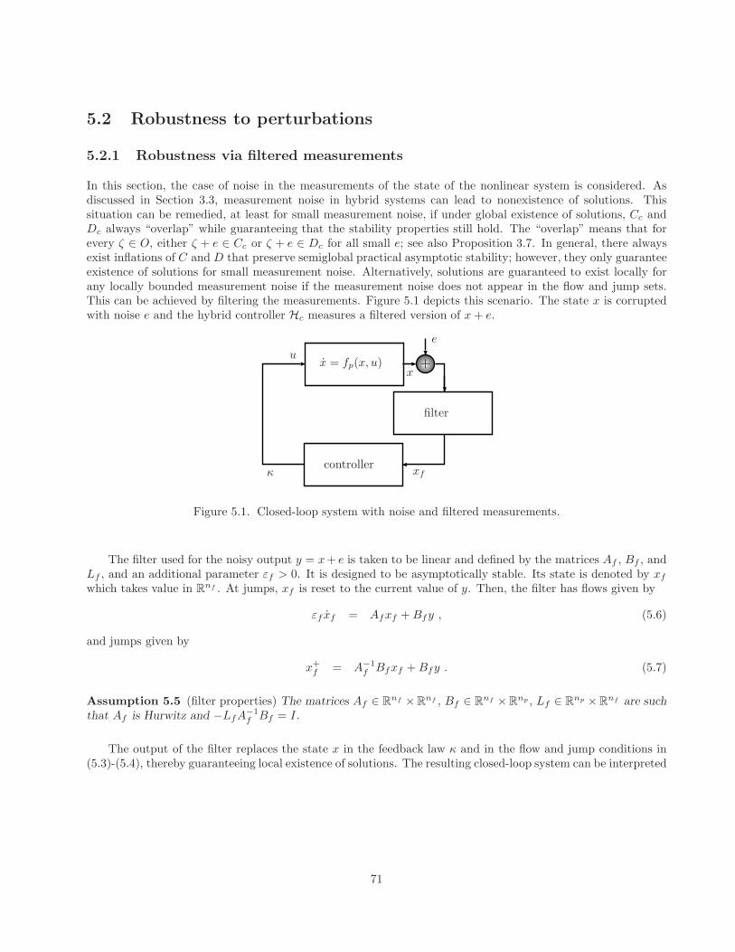
5.2 Robustness to perturbations

5.2.1 Robustness via filtered measurements

In this section, the case of noise in the measurements of the state of the nonlinear system is considered. Asdiscussed in Section 3.3, measurement noise in hybrid systems can lead to nonexistence of solutions. Thissituation can be remedied, at least for small measurement noise, if under global existence of solutions, Cc andDc always “overlap” while guaranteeing that the stability properties still hold. The “overlap” means that forevery ζ ∈ O, either ζ + e ∈ Cc or ζ + e ∈ Dc for all small e; see also Proposition 3.7. In general, there alwaysexist inflations of C and D that preserve semiglobal practical asymptotic stability; however, they only guaranteeexistence of solutions for small measurement noise. Alternatively, solutions are guaranteed to exist locally forany locally bounded measurement noise if the measurement noise does not appear in the flow and jump sets.This can be achieved by filtering the measurements. Figure 5.1 depicts this scenario. The state x is corruptedwith noise e and the hybrid controller Hc measures a filtered version of x+ e.

x = fp(x, u)x

u

e

xfκ

filter

controller

Figure 5.1. Closed-loop system with noise and filtered measurements.

The filter used for the noisy output y = x+ e is taken to be linear and defined by the matrices Af , Bf , andLf , and an additional parameter εf > 0. It is designed to be asymptotically stable. Its state is denoted by xf

which takes value in Rnf . At jumps, xf is reset to the current value of y. Then, the filter has flows given by

εf xf = Afxf +Bfy , (5.6)

and jumps given by

x+f = A−1

f Bfxf +Bfy . (5.7)

Assumption 5.5 (filter properties) The matrices Af ∈ Rnf ×R

nf , Bf ∈ Rnf ×R

np , Lf ∈ Rnp ×R

nf are suchthat Af is Hurwitz and −LfA

−1f Bf = I.

The output of the filter replaces the state x in the feedback law κ and in the flow and jump conditions in(5.3)-(5.4), thereby guaranteeing local existence of solutions. The resulting closed-loop system can be interpreted

71

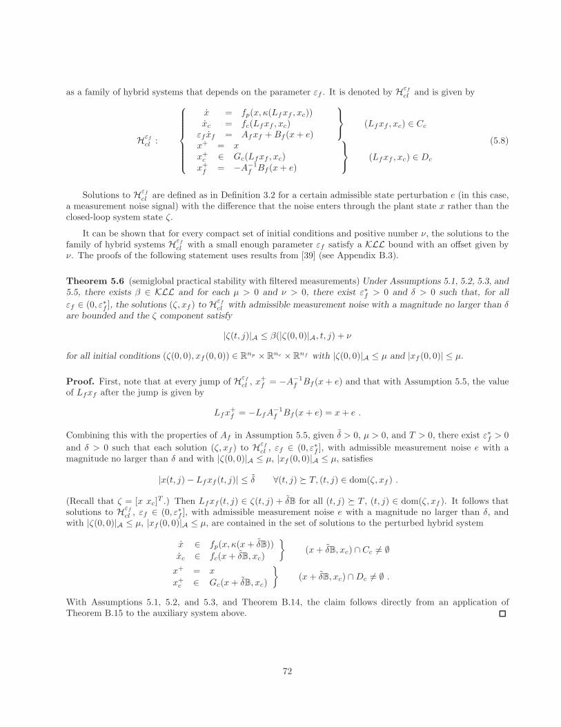
as a family of hybrid systems that depends on the parameter εf . It is denoted by Hεf

cl and is given by

Hεf

cl :

x = fp(x, κ(Lfxf , xc))xc = fc(Lfxf , xc)εf xf = Afxf +Bf (x+ e)

(Lfxf , xc) ∈ Cc

x+ = xx+

c ∈ Gc(Lfxf , xc)x+

f = −A−1f Bf (x+ e)

(Lfxf , xc) ∈ Dc

(5.8)

Solutions to Hεf

cl are defined as in Definition 3.2 for a certain admissible state perturbation e (in this case,a measurement noise signal) with the difference that the noise enters through the plant state x rather than theclosed-loop system state ζ.

It can be shown that for every compact set of initial conditions and positive number ν, the solutions to thefamily of hybrid systems Hεf

cl with a small enough parameter εf satisfy a KLL bound with an offset given byν. The proofs of the following statement uses results from [39] (see Appendix B.3).

Theorem 5.6 (semiglobal practical stability with filtered measurements) Under Assumptions 5.1, 5.2, 5.3, and5.5, there exists β ∈ KLL and for each µ > 0 and ν > 0, there exist ε∗f > 0 and δ > 0 such that, for all

εf ∈ (0, ε∗f ], the solutions (ζ, xf ) to Hεf

cl with admissible measurement noise with a magnitude no larger than δare bounded and the ζ component satisfy

|ζ(t, j)|A ≤ β(|ζ(0, 0)|A, t, j) + ν

for all initial conditions (ζ(0, 0), xf (0, 0)) ∈ Rnp × R

nc × Rnf with |ζ(0, 0)|A ≤ µ and |xf (0, 0)| ≤ µ.

Proof. First, note that at every jump of Hεf

cl , x+f = −A−1

f Bf (x+ e) and that with Assumption 5.5, the valueof Lfxf after the jump is given by

Lfx+f = −LfA

−1f Bf (x+ e) = x+ e .

Combining this with the properties of Af in Assumption 5.5, given δ > 0, µ > 0, and T > 0, there exist ε∗f > 0

and δ > 0 such that each solution (ζ, xf ) to Hεf

cl , εf ∈ (0, ε∗f ], with admissible measurement noise e with amagnitude no larger than δ and with |ζ(0, 0)|A ≤ µ, |xf (0, 0)|A ≤ µ, satisfies

|x(t, j) − Lfxf (t, j)| ≤ δ ∀(t, j) T, (t, j) ∈ dom(ζ, xf ) .

(Recall that ζ = [x xc]T .) Then Lfxf (t, j) ∈ ζ(t, j) + δB for all (t, j) T , (t, j) ∈ dom(ζ, xf ). It follows that

solutions to Hεf

cl , εf ∈ (0, ε∗f ], with admissible measurement noise e with a magnitude no larger than δ, andwith |ζ(0, 0)|A ≤ µ, |xf (0, 0)|A ≤ µ, are contained in the set of solutions to the perturbed hybrid system

x ∈ fp(x, κ(x+ δB))

xc ∈ fc(x+ δB, xc)

(x+ δB, xc) ∩ Cc 6= ∅

x+ = x

x+c ∈ Gc(x+ δB, xc)

(x+ δB, xc) ∩Dc 6= ∅ .

With Assumptions 5.1, 5.2, and 5.3, and Theorem B.14, the claim follows directly from an application ofTheorem B.15 to the auxiliary system above.

72

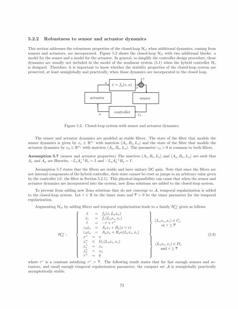
5.2.2 Robustness to sensor and actuator dynamics

This section addresses the robustness properties of the closed-loop Hcl when additional dynamics, coming fromsensors and actuators, are incorporated. Figure 5.2 shows the closed-loop Hcl with two additional blocks: amodel for the sensor and a model for the actuator. In general, to simplify the controller design procedure, thesedynamics are usually not included in the model of the nonlinear system (5.1) when the hybrid controller Hc

is designed. Therefore, it is important to know whether the stability properties of the closed-loop system arepreserved, at least semiglobally and practically, when those dynamics are incorporated in the closed loop.

x = fp(x, u)x

ue

xsκ

sensoractuator

controller

Figure 5.2. Closed-loop system with sensor and actuator dynamics.

The sensor and actuator dynamics are modeled as stable filters. The state of the filter that models thesensor dynamics is given by xs ∈ R

ns with matrices (As, Bs, Ls) and the state of the filter that models theactuator dynamics by xa ∈ R

na with matrices (Aa, Ba, La). The parameter εd > 0 is common to both filters.

Assumption 5.7 (sensor and actuator properties) The matrices (As, Bs, Ls) and (Aa, Ba, La) are such thatAs and Aa are Hurwitz, −LsA

−1s Bs = I and −LaA

−1a Ba = I.

Assumption 5.7 states that the filters are stable and have unitary DC gain. Note that since the filters arenot internal components of the hybrid controller, their state cannot be reset at jumps to an arbitrary value givenby the controller (cf. the filter in Section 5.2.1). This physical impossibility can cause that when the sensor andactuator dynamics are incorporated into the system, new Zeno solutions are added to the closed-loop system.

To prevent from adding new Zeno solutions that do not converge to A, temporal regularization is addedto the closed-loop system. Let τ ∈ R be the timer state and τ > 0 be the timer parameter for the temporalregularization.

Augmenting Hcl by adding filters and temporal regularization leads to a family Hεd

cl given as follows

Hεd

cl :

x = fp(x, Laxa)xc = fc(Lsxs, xc)τ = −τ + τ∗

εdxs = Asxs +Bs(x+ e)εdxa = Aaxa +Baκ(Lsxs, xc)

(Lsxs, xc) ∈ Cc

or τ ≤ τ

x+ = xx+

c ∈ Gc(Lsxs, xc)x+

s = xs

x+a = xa

τ+ = 0

(Lsxs, xc) ∈ Dc

and τ ≥ τ

(5.9)

where τ∗ is a constant satisfying τ∗ > τ . The following result states that for fast enough sensors and ac-tuators, and small enough temporal regularization parameter, the compact set A is semiglobally practicallyasymptotically stable.

73

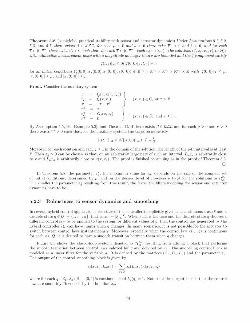
Theorem 5.8 (semiglobal practical stability with sensor and actuator dynamics) Under Assumptions 5.1, 5.2,5.3, and 5.7, there exists β ∈ KLL, for each µ > 0 and ν > 0 there exist τ∗ > 0 and δ > 0, and for eachτ ∈ (0, τ∗] there exist ε∗d > 0 such that, for each τ ∈ (0, τ∗], each εd ∈ (0, ε∗d], the solutions (ζ, xs, xa, τ) to Hεd

cl

with admissible measurement noise with a magnitude no larger than δ are bounded and the ζ component satisfy

|ζ(t, j)|A ≤ β(|ζ(0, 0)|A, t, j) + ν

for all initial conditions (ζ(0, 0), xs(0, 0), xa(0, 0), τ(0, 0)) ∈ Rnp × R

nc × Rns × R

na × R with |ζ(0, 0)|A ≤ µ,|xs(0, 0)| ≤ µ, and |xa(0, 0)| ≤ µ.

Proof. Consider the auxiliary system

x = fp(x, κ(x, xc))xc = fc(x, xc)τ = −τ + τ∗

(x, xc) ∈ Cc or τ ≤ τ

x+ = xx+

c ∈ Gc(x, xc)τ+ = 0

(x, xc) ∈ Dc and τ ≥ τ .

By Assumption 5.5, [39, Example 5.3], and Theorem B.14 there exists β ∈ KLL and for each µ > 0 and ν > 0there exists τ∗ > 0 such that, for the auxiliary system, the trajectories satisfy

|z(t, j)|A ≤ β(|z(0, 0)|A, t, j) +ν

2.

Moreover, for each solution and each j ≥ 1 in the domain of the solution, the length of the j-th interval is at leastτ . Then ε∗d > 0 can be chosen so that, on an arbitrarily large part of such an interval, Lsxs is arbitrarily closeto x and Laxa is arbitrarily close to κ(x, xc). The proof is finished continuing as in the proof of Theorem 5.6.

In Theorem 5.8, the parameter ε∗d, the maximum value for εd, depends on the size of the compact setof initial conditions, determined by µ, and on the desired level of closeness ν to A for the solutions to Hεd

cl .The smaller the parameter ε∗d resulting from this result, the faster the filters modeling the sensor and actuatordynamics have to be.

5.2.3 Robustness to sensor dynamics and smoothing

In several hybrid control applications, the state of the controller is explicitly given as a continuous state ξ and adiscrete state q ∈ Q := 1, . . . , n, that is, xc := [ξ q]T . When such is the case and the discrete state q chooses adifferent control law to be applied to the system for different values of q, then the control law generated by thehybrid controller Hc can have jumps when q changes. In many scenarios, it is not possible for the actuator toswitch between control laws instantaneously. Moreover, especially when the control law κ(·, ·, q) is continuousfor each q ∈ Q, it is desired to have a smooth transition between them when q changes.

Figure 5.3 shows the closed-loop system, denoted as Hεu

cl , resulting from adding a block that performsthe smooth transition between control laws indexed by’ q and denoted by κq. The smoothing control block ismodeled as a linear filter for the variable q. It is defined by the matrices (Au, Bu, Lu) and the parameter εu.The output of the control smoothing block is given by

α(x, xc, Luxu) =∑

q∈Q

λq(Luxu)κ(x, xc, q)

where for each q ∈ Q, λq : R → [0, 1] is continuous and λq(q) = 1. Note that the output is such that the controllaws are smoothly “blended” by the function λq.

74

Assumption 5.9 (actuator smoothing properties) The matrices (Au, Bu, Lu) are such that Au is Hurwitz,−LuA

−1u Bu = I.

The smoothing block is considered to be part of the actuator, and for that reason, it is not possible to resetits state at jumps. In addition to this block, a filter modeling the sensor dynamics is also incorporated as inSection 5.2.2. The closed loop Hεu

cl can be written as

Hεu

cl :

x = fp(x, α(x, xc, Luxu))

ξ = fc(Lsxs, xc)q = 0τ = −τ + τ∗

εuxs = Asxs +Bs(x)εuxu = Auxu +Buq

(Lsxs, xc) ∈ Cc or τ ≤ τ

x+ = x[ξ+

q+

]+

∈ Gc(Lsxs, xc)

x+s = xs

x+u = xu

τ+ = 0

(Lsxs, xc) ∈ Dc

and τ ≥ τ .

(5.10)

Theorem 5.10 (semiglobal practical stability with actuator smoothing) Under Assumptions 5.1, 5.2, 5.3, and5.9, there exists β ∈ KLL, for each µ > 0 and ν > 0 there exist τ∗ > 0, and for each τ ∈ (0, τ∗] there existε∗u > 0 such that, for each τ ∈ (0, τ∗], each εu ∈ (0, ε∗u], the solutions (ζ, xs, xu, τ) to Hεu

cl are bounded and theζ component satisfy

|ζ(t, j)|A ≤ β(|ζ(0, 0)|A, t, j) + ν

for all initial conditions (ζ(0, 0), xs(0, 0), xu(0, 0), τ(0, 0)) ∈ Rnp × R

nc × Rna × R with |ζ(0, 0)|A ≤ µ, and

|xu(0, 0)| ≤ µ.

A corollary to Theorem 5.10 establishing robustness to noise in the state x (as in Theorem 5.6) also holdsfor the closed-loop system with control smoothing Hεu

cl .

In Section 5.4, we add fast sensor dynamics and control smoothing to the problem of swinging up a pendulumon a cart.

x = fp(x, u)u

xs

κ1 κnq

sensor

controller

smoothing

Figure 5.3. Closed-loop system with sensor dynamics and control smoothing.

75

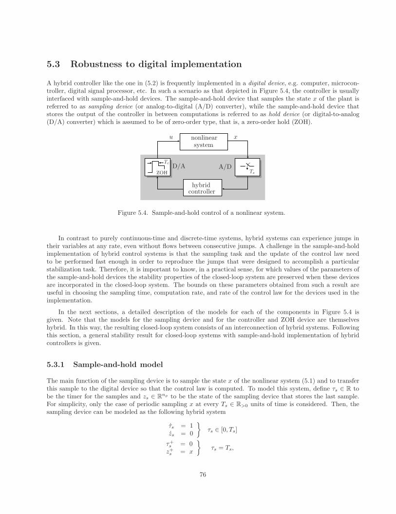
5.3 Robustness to digital implementation

A hybrid controller like the one in (5.2) is frequently implemented in a digital device, e.g. computer, microcon-troller, digital signal processor, etc. In such a scenario as that depicted in Figure 5.4, the controller is usuallyinterfaced with sample-and-hold devices. The sample-and-hold device that samples the state x of the plant isreferred to as sampling device (or analog-to-digital (A/D) converter), while the sample-and-hold device thatstores the output of the controller in between computations is referred to as hold device (or digital-to-analog(D/A) converter) which is assumed to be of zero-order type, that is, a zero-order hold (ZOH).

Tc

Ts

xu

D/A A/D

controller

nonlinear

hybrid

system

ZOH

Figure 5.4. Sample-and-hold control of a nonlinear system.

In contrast to purely continuous-time and discrete-time systems, hybrid systems can experience jumps intheir variables at any rate, even without flows between consecutive jumps. A challenge in the sample-and-holdimplementation of hybrid control systems is that the sampling task and the update of the control law needto be performed fast enough in order to reproduce the jumps that were designed to accomplish a particularstabilization task. Therefore, it is important to know, in a practical sense, for which values of the parameters ofthe sample-and-hold devices the stability properties of the closed-loop system are preserved when these devicesare incorporated in the closed-loop system. The bounds on these parameters obtained from such a result areuseful in choosing the sampling time, computation rate, and rate of the control law for the devices used in theimplementation.

In the next sections, a detailed description of the models for each of the components in Figure 5.4 isgiven. Note that the models for the sampling device and for the controller and ZOH device are themselveshybrid. In this way, the resulting closed-loop system consists of an interconnection of hybrid systems. Followingthis section, a general stability result for closed-loop systems with sample-and-hold implementation of hybridcontrollers is given.

5.3.1 Sample-and-hold model

The main function of the sampling device is to sample the state x of the nonlinear system (5.1) and to transferthis sample to the digital device so that the control law is computed. To model this system, define τs ∈ R tobe the timer for the samples and zs ∈ R

np to be the state of the sampling device that stores the last sample.For simplicity, only the case of periodic sampling x at every Ts ∈ R>0 units of time is considered. Then, thesampling device can be modeled as the following hybrid system

τs = 1zs = 0

τs ∈ [0, Ts]

τ+s = 0z+

s = x

τs = Ts,

76

where the continuous dynamics are such that the timer counts the time elapsed from the last jump and thesampling state zs is kept constant as long as τs ∈ [0, Ts]. When τs = Ts, flows are no longer possible, jumps areforced, and are such that the timer is updated to zero, and the sampling state is updated to the current valueof the state x.

The digital controller performs the actual computation of the control algorithm in Hc and updates thestate of the ZOH device, which are denoted by zc ∈ R

nc . These are modeled as a single hybrid system Hh−c.Synchrony between this system and the sampling device is not assumed, i.e., the computation of the algorithmand the update of the ZOH are governed by an independent clock, which in general, has a different samplingtime than the sampling device. The model for Hh−c is given in terms of the ZOH state zc ∈ R

nc which storesthe computation resulting from the controller Hc, a timer state τc ∈ R which after very Tc ∈ R>0 units of time,triggers the computation of the control algorithm and updates the ZOH. Since there is no synchronization withthe sampling device and no relationship between the constants τs and τc a priori, it could be the case thatthe sampling device is updated in between computations. To accommodate to this situation, a memory statezm ∈ R

np is added to the model in order to store the samples provided by the sampling device. With thesedefinitions, the model of Hh−c, that is, the digital controller with the hold device, is given by

τc = 1zc = 0zm = 0

τc ∈ [0, Tc]

τ+c = 0z+

c ∈ gHc(zm, zc)

z+m = zs

τc = Tc

where gHcis defined below.

These dynamics are such that when τc ∈ [0, Tc], the timer τc counts the elapsed time and the states zc andzm remain constant. When τc = Tc then the timer is reset to zero, the output of the ZOH device zc is updated,and the memory state zm is updated to the last sample zs. The update law for zc is given by

gHc(zm, zc) :=

gfc(zm, zc) (zm, zc) ∈ Cc \Dc

Gc(zm, zc) (zm, zc) ∈ Dc \ Cc

gfc(zm, zc), Gc(zm, zc) (zm, zc) ∈ Cc ∩Dc

(5.11)

where gfcis an approximation of the flow equation of Hc, and Gc is the same jump mapping as for Hc.

5.3.2 Closed-loop system analysis

The closed-loop system with the models for the nonlinear system, sampling device, and digital controller and

ZOH device given in Section 5.3.1 is denoted by HS/Hcl ; has states x, zc, zs, τs, τc, zm; has continuous dynamics

given by

x = fp(x, κ(zs, zc))zc = 0zs = 0τs = 1τc = 1zm = 0

τs ∈ [0, Ts] and τc ∈ [0, Tc];

77

and discrete dynamics given by

x+

z+c

z+s

τ+s

τ+c

z+m

=

xzc

x0τczm

=: g1(x, zc, zs, τs, τc, zm)

when τs = Ts and τc ∈ [0, Tc),

x+

z+c

z+s

τ+s

τ+c

z+m

∈

xgHc

(zm, zc)zs

τs0zs

=: g2(x, zc, zs, τs, τc, zm)

when τs ∈ [0, Ts) and τc = Tc, and

x+

z+c

z+s

τ+s

τ+c

z+m

∈ g1(x, zc, zs, τs, τc, zm), g2(x, zc, zs, τs, τc, zm)

when τc = Tc and τs ∈ Ts. The flows of the closed loop are governed by the flow equation of each subsystem.The jump mappings are combined so that only the states of the original jump mapping are updated. Forinstance, when τs = Ts and τc ∈ [0, Tc), only the states zs and τs are updated to new values (as discussed inSection 5.3.1) while the other states are mapped back to their current values. Moreover, note that the data of

HS/Hcl satisfy the hybrid basic conditions.

It is expected that, in order to establish any type of stability result for HS/Hcl inherited from the stability

properties of Hcl, the value of the flows of Hc and the value of gfcin the controller’s jump mapping gHc

haveto be “close” at jumps. The consistency property defined below is one way to guarantee such closeness.

Given two positive real numbers δ and ∆ satisfying 0 < δ ≤ ∆ <∞ and a compact set A ⊂ Rn+nc , define

ΩA(δ,∆) := (x, xc) ∈ Rnp × R

nc | δ ≤ |(x, xc)|A ≤ ∆ .

Definition 5.11 (consistency of flow map of Hc) Let A be a compact subset of Rnp × R

nc . The integrationscheme gfc

is said to be consistent with respect to fc if for each positive number ∆s there exists ρ ∈ K∞ andT ′

c > 0 such that for each (x0, x0c) ∈ ΩA(0,∆s) and each Tc ∈ (0, T ′

c) there exists a solution ϕ(t) to ϕ = fc(x, ϕ),ϕ(0) = x0

c , with x(t) satisfying x = fp(x, κ(x0, ϕ(0))), x(0) = x0, such that

|gfc(x(0), ϕ(0)) − ϕ(Tc)| ≤ Tcρ(Tc) . (5.12)

Theorem 5.12 (semiglobal practical stability) Let Assumption 5.1, 5.2, and 5.3 hold. Let the integrationscheme gfc

in Hcl be consistent with respect to fc. Then, the set A is semiglobally practically asymptotically

stable for HS/Hcl , i.e. there exists β ∈ KLL, for every compact set K ⊂ R

np × Rnc and every ε > 0 there

78

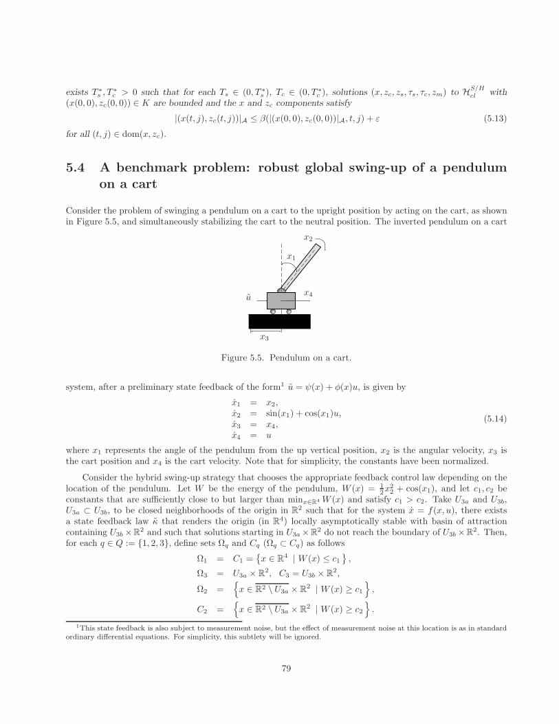
exists T ∗s , T

∗c > 0 such that for each Ts ∈ (0, T ∗

s ), Tc ∈ (0, T ∗c ), solutions (x, zc, zs, τs, τc, zm) to HS/H

cl with(x(0, 0), zc(0, 0)) ∈ K are bounded and the x and zc components satisfy

|(x(t, j), zc(t, j))|A ≤ β(|(x(0, 0), zc(0, 0))|A, t, j) + ε (5.13)

for all (t, j) ∈ dom(x, zc).

5.4 A benchmark problem: robust global swing-up of a pendulumon a cart

Consider the problem of swinging a pendulum on a cart to the upright position by acting on the cart, as shownin Figure 5.5, and simultaneously stabilizing the cart to the neutral position. The inverted pendulum on a cart

x1

x2

x3

x4u

Figure 5.5. Pendulum on a cart.

system, after a preliminary state feedback of the form1 u = ψ(x) + φ(x)u, is given by

x1 = x2,x2 = sin(x1) + cos(x1)u,x3 = x4,x4 = u

(5.14)

where x1 represents the angle of the pendulum from the up vertical position, x2 is the angular velocity, x3 isthe cart position and x4 is the cart velocity. Note that for simplicity, the constants have been normalized.

Consider the hybrid swing-up strategy that chooses the appropriate feedback control law depending on thelocation of the pendulum. Let W be the energy of the pendulum, W (x) = 1

2x22 + cos(x1), and let c1, c2 be

constants that are sufficiently close to but larger than minx∈R4 W (x) and satisfy c1 > c2. Take U3a and U3b,U3a ⊂ U3b, to be closed neighborhoods of the origin in R

2 such that for the system x = f(x, u), there existsa state feedback law κ that renders the origin (in R

4) locally asymptotically stable with basin of attractioncontaining U3b ×R

2 and such that solutions starting in U3a ×R2 do not reach the boundary of U3b ×R

2. Then,for each q ∈ Q := 1, 2, 3, define sets Ωq and Cq (Ωq ⊂ Cq) as follows

Ω1 = C1 =x ∈ R

4 | W (x) ≤ c1,

Ω3 = U3a × R2, C3 = U3b × R

2,

Ω2 =x ∈ R2 \ U3a × R

2 | W (x) ≥ c1

,

C2 =x ∈ R2 \ U3a × R

2 | W (x) ≥ c2

.

1This state feedback is also subject to measurement noise, but the effect of measurement noise at this location is as in standardordinary differential equations. For simplicity, this subtlety will be ignored.

79

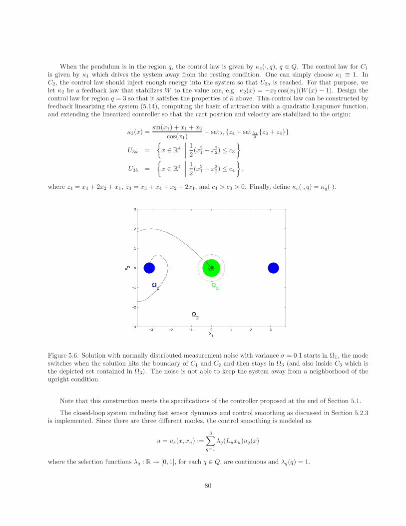
When the pendulum is in the region q, the control law is given by κc(·, q), q ∈ Q. The control law for C1

is given by κ1 which drives the system away from the resting condition. One can simply choose κ1 ≡ 1. InC2, the control law should inject enough energy into the system so that U3a is reached. For that purpose, welet κ2 be a feedback law that stabilizes W to the value one, e.g. κ2(x) = −x2 cos(x1)(W (x) − 1). Design thecontrol law for region q = 3 so that it satisfies the properties of κ above. This control law can be constructed byfeedback linearizing the system (5.14), computing the basin of attraction with a quadratic Lyapunov function,and extending the linearized controller so that the cart position and velocity are stabilized to the origin:

κ3(x) =sin(x1) + x1 + x2

cos(x1)+ satλ1z4 + satλ1

2z3 + z4

U3a =

x ∈ R

4

∣∣∣∣1

2(x2

1 + x22) ≤ c3

U3b =

x ∈ R

4

∣∣∣∣1

2(x2

1 + x22) ≤ c4

,

where z4 = x4 + 2x2 + x1, z3 = x3 + x4 + x2 + 2x1, and c4 > c3 > 0. Finally, define κc(·, q) = κq(·).

−3 −2 −1 0 1 2 3−3

−2

−1

0

1

2

3

Ω1

x1

x 2

Ω2

Ω1

Ω3

Figure 5.6. Solution with normally distributed measurement noise with variance σ = 0.1 starts in Ω1, the modeswitches when the solution hits the boundary of C1 and C2 and then stays in Ω3 (and also inside C3 which isthe depicted set contained in Ω3). The noise is not able to keep the system away from a neighborhood of theupright condition.

Note that this construction meets the specifications of the controller proposed at the end of Section 5.1.

The closed-loop system including fast sensor dynamics and control smoothing as discussed in Section 5.2.3is implemented. Since there are three different modes, the control smoothing is modeled as

u = us(x, xu) :=3∑

q=1

λq(Luxu)uq(x)

where the selection functions λq : R → [0, 1], for each q ∈ Q, are continuous and λq(q) = 1.

80

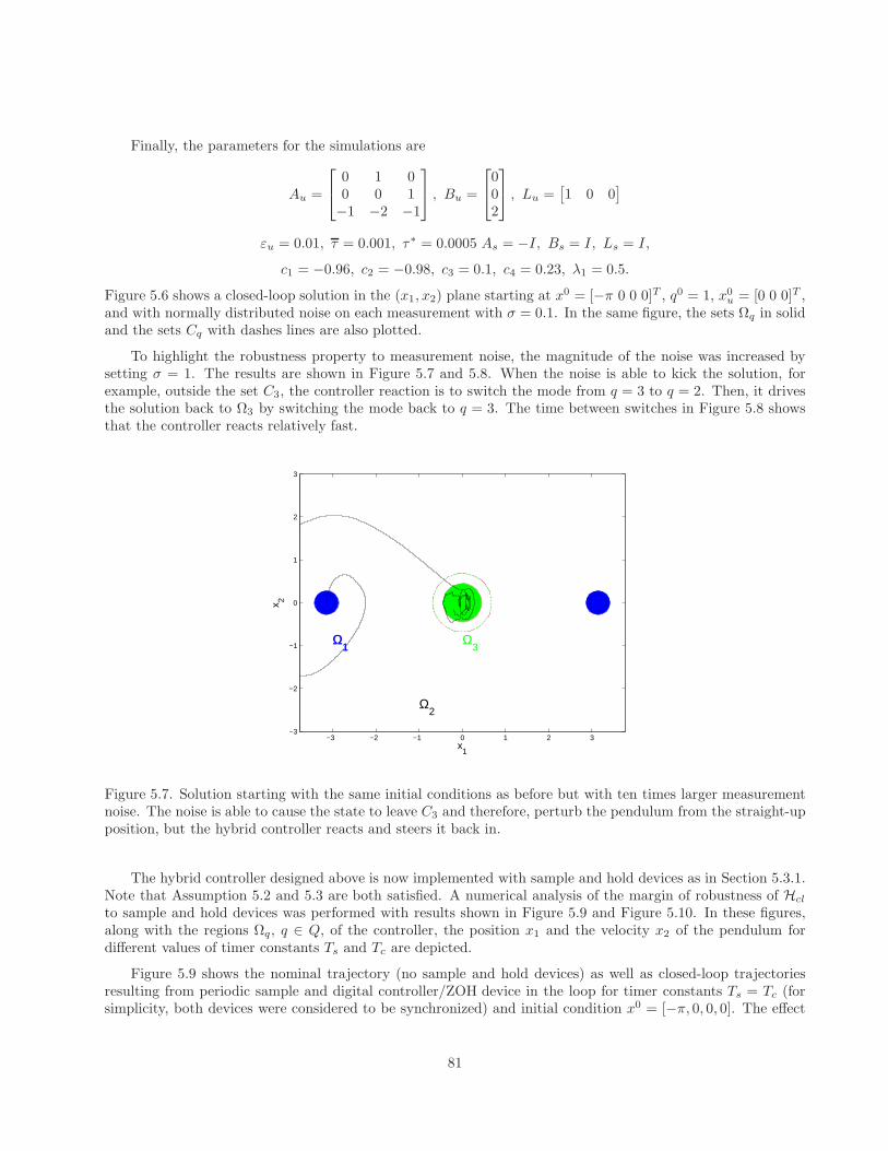
Finally, the parameters for the simulations are

Au =

0 1 00 0 1−1 −2 −1

, Bu =

002

, Lu =

[1 0 0

]

εu = 0.01, τ = 0.001, τ∗ = 0.0005 As = −I, Bs = I, Ls = I,

c1 = −0.96, c2 = −0.98, c3 = 0.1, c4 = 0.23, λ1 = 0.5.

Figure 5.6 shows a closed-loop solution in the (x1, x2) plane starting at x0 = [−π 0 0 0]T , q0 = 1, x0u = [0 0 0]T ,

and with normally distributed noise on each measurement with σ = 0.1. In the same figure, the sets Ωq in solidand the sets Cq with dashes lines are also plotted.

To highlight the robustness property to measurement noise, the magnitude of the noise was increased bysetting σ = 1. The results are shown in Figure 5.7 and 5.8. When the noise is able to kick the solution, forexample, outside the set C3, the controller reaction is to switch the mode from q = 3 to q = 2. Then, it drivesthe solution back to Ω3 by switching the mode back to q = 3. The time between switches in Figure 5.8 showsthat the controller reacts relatively fast.

−3 −2 −1 0 1 2 3−3

−2

−1

0

1

2

3

Ω1

x1

x 2

Ω2

Ω1

Ω3

Figure 5.7. Solution starting with the same initial conditions as before but with ten times larger measurementnoise. The noise is able to cause the state to leave C3 and therefore, perturb the pendulum from the straight-upposition, but the hybrid controller reacts and steers it back in.

The hybrid controller designed above is now implemented with sample and hold devices as in Section 5.3.1.Note that Assumption 5.2 and 5.3 are both satisfied. A numerical analysis of the margin of robustness of Hcl

to sample and hold devices was performed with results shown in Figure 5.9 and Figure 5.10. In these figures,along with the regions Ωq, q ∈ Q, of the controller, the position x1 and the velocity x2 of the pendulum fordifferent values of timer constants Ts and Tc are depicted.

Figure 5.9 shows the nominal trajectory (no sample and hold devices) as well as closed-loop trajectoriesresulting from periodic sample and digital controller/ZOH device in the loop for timer constants Ts = Tc (forsimplicity, both devices were considered to be synchronized) and initial condition x0 = [−π, 0, 0, 0]. The effect

81

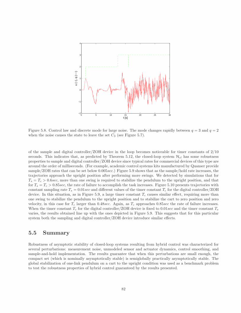
0 5 10 15 20 25 30−2

−1

0

1

2

3

4

t [s]

u (−

), q

(−

−)

Figure 5.8. Control law and discrete mode for large noise. The mode changes rapidly between q = 3 and q = 2when the noise causes the state to leave the set C3 (see Figure 5.7).

of the sample and digital controller/ZOH device in the loop becomes noticeable for timer constants of 2/10seconds. This indicates that, as predicted by Theorem 5.12, the closed-loop system Hcl has some robustnessproperties to sample and digital controller/ZOH device since typical rates for commercial devices of this type arearound the order of milliseconds. (For example, academic control systems kits manufactured by Quanser providesample/ZOH rates that can be set below 0.005sec.) Figure 5.9 shows that as the sample/hold rate increases, thetrajectories approach the upright position after performing more swings. We detected by simulations that forTs = Tc > 0.6sec, more than one swing is required to stabilize the pendulum to the upright position, and thatfor Ts = Tc > 0.85sec, the rate of failure to accomplish the task increases. Figure 5.10 presents trajectories withconstant sampling rate Ts = 0.01sec and different values of the timer constant Tc for the digital controller/ZOHdevice. In this situation, as in Figure 5.9, a large timer constant Tc causes similar effect, requiring more thanone swing to stabilize the pendulum to the upright position and to stabilize the cart to zero position and zerovelocity, in this case for Tc larger than 0.48sec. Again, as Tc approaches 0.85sec the rate of failure increases.When the timer constant Tc for the digital controller/ZOH device is fixed to 0.01sec and the timer constant Ts

varies, the results obtained line up with the ones depicted in Figure 5.9. This suggests that for this particularsystem both the sampling and digital controller/ZOH device introduce similar effects.

5.5 Summary

Robustness of asymptotic stability of closed-loop systems resulting from hybrid control was characterized forseveral perturbations: measurement noise, unmodeled sensor and actuator dynamics, control smoothing, andsample-and-hold implementation. The results guarantee that when this perturbations are small enough, thecompact set (which is nominally asymptotically stable) is semiglobally practically asymptotically stable. Theglobal stabilization of one-link pendulum on a cart to the upright condition was used as a benchmark problemto test the robustness properties of hybrid control guaranteed by the results presented.

82

−6 −4 −2 0 2 4 6

−4

−3

−2

−1

0

1

2

3

4

x1

x 2

Ω2

Ω1

Ω3

nominal

Figure 5.9. Closed-loop trajectories for the nominal case (no sample and hold devices) and for timer constants:Ts = Tc = 0.2sec (:), Ts = Tc = 0.6sec (−.), Ts = Tc = 0.8sec (−−), Ts = Tc = 0.85sec (solid).

−6 −4 −2 0 2 4 6

−4

−3

−2

−1

0

1

2

3

4

Ω1

x1

x 2

Ω2

Ω3

nominal

Figure 5.10. Closed-loop trajectories for the nominal case (solid) and for (fixed) timer constant of the samplerTs = 0.01sec and for timer constants of the digital controller/ZOH device: Tc = 0.2sec (:), Tc = 0.48sec (−.),Tc = 0.8sec (−−), Tc = 0.85sec (solid).


For references showing that it is impossible to stabilize nonholonomic using time-invariant continuous statefeedback and robust stabilization is impossible using time-invariant locally bounded feedback see, for example,

83

[49, 76].

The robustness properties inherited when sample and hold control is used in stabilization is discussed in[95, 28, 53].

Consistency properties have been considered for numerical integration schemes in the numerical analysisliterature (see e.g. [96, 5]) and in the construction of approximate models for discrete-time systems (see e.g.[75]).

The ideas in the particular hybrid controller at the end of Section 5.1 are similar to the ones in [77].

For swing up of a pendulum on a cart control algorithms related to the one in Section 5.4 see, for example,[6, 102, 26].

The preliminary state feedback and the construction of κ in Section 5.4 are, for example, given in [99] .

The proof of 5.12 is given in Section B.3.

84

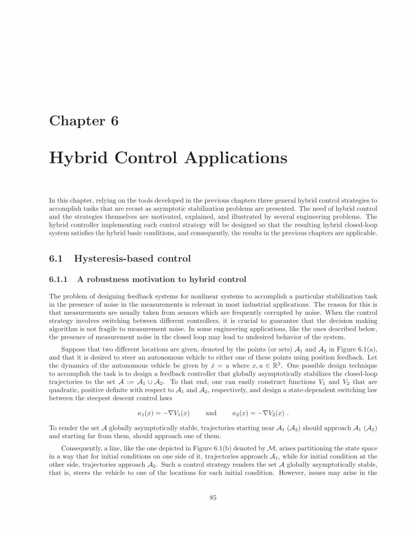
Chapter 6

Hybrid Control Applications

In this chapter, relying on the tools developed in the previous chapters three general hybrid control strategies toaccomplish tasks that are recast as asymptotic stabilization problems are presented. The need of hybrid controland the strategies themselves are motivated, explained, and illustrated by several engineering problems. Thehybrid controller implementing each control strategy will be designed so that the resulting hybrid closed-loopsystem satisfies the hybrid basic conditions, and consequently, the results in the previous chapters are applicable.

6.1 Hysteresis-based control

6.1.1 A robustness motivation to hybrid control

The problem of designing feedback systems for nonlinear systems to accomplish a particular stabilization taskin the presence of noise in the measurements is relevant in most industrial applications. The reason for this isthat measurements are usually taken from sensors which are frequently corrupted by noise. When the controlstrategy involves switching between different controllers, it is crucial to guarantee that the decision makingalgorithm is not fragile to measurement noise. In some engineering applications, like the ones described below,the presence of measurement noise in the closed loop may lead to undesired behavior of the system.

Suppose that two different locations are given, denoted by the points (or sets) A1 and A2 in Figure 6.1(a),and that it is desired to steer an autonomous vehicle to either one of these points using position feedback. Letthe dynamics of the autonomous vehicle be given by x = u where x, u ∈ R

2. One possible design techniqueto accomplish the task is to design a feedback controller that globally asymptotically stabilizes the closed-looptrajectories to the set A := A1 ∪ A2. To that end, one can easily construct functions V1 and V2 that arequadratic, positive definite with respect to A1 and A2, respectively, and design a state-dependent switching lawbetween the steepest descent control laws

κ1(x) = −∇V1(x) and κ2(x) = −∇V2(x) .

To render the set A globally asymptotically stable, trajectories starting near A1 (A2) should approach A1 (A2)and starting far from them, should approach one of them.

Consequently, a line, like the one depicted in Figure 6.1(b) denoted by M, arises partitioning the state spacein a way that for initial conditions on one side of it, trajectories approach A1, while for initial condition at theother side, trajectories approach A2. Such a control strategy renders the set A globally asymptotically stable,that is, steers the vehicle to one of the locations for each initial condition. However, issues may arise in the

85

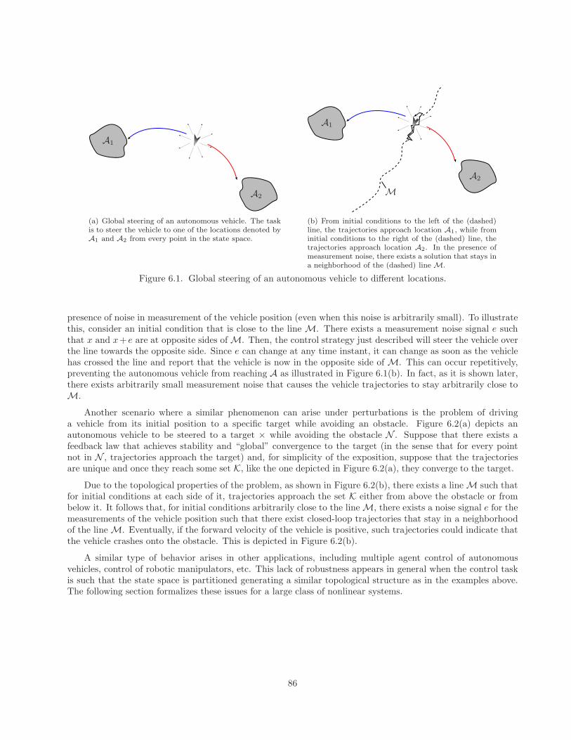
A2

A1

(a) Global steering of an autonomous vehicle. The taskis to steer the vehicle to one of the locations denoted byA1 and A2 from every point in the state space.

MA2

A1

(b) From initial conditions to the left of the (dashed)line, the trajectories approach location A1, while frominitial conditions to the right of the (dashed) line, thetrajectories approach location A2. In the presence ofmeasurement noise, there exists a solution that stays ina neighborhood of the (dashed) line M.

Figure 6.1. Global steering of an autonomous vehicle to different locations.

presence of noise in measurement of the vehicle position (even when this noise is arbitrarily small). To illustratethis, consider an initial condition that is close to the line M. There exists a measurement noise signal e suchthat x and x+ e are at opposite sides of M. Then, the control strategy just described will steer the vehicle overthe line towards the opposite side. Since e can change at any time instant, it can change as soon as the vehiclehas crossed the line and report that the vehicle is now in the opposite side of M. This can occur repetitively,preventing the autonomous vehicle from reaching A as illustrated in Figure 6.1(b). In fact, as it is shown later,there exists arbitrarily small measurement noise that causes the vehicle trajectories to stay arbitrarily close toM.

Another scenario where a similar phenomenon can arise under perturbations is the problem of drivinga vehicle from its initial position to a specific target while avoiding an obstacle. Figure 6.2(a) depicts anautonomous vehicle to be steered to a target × while avoiding the obstacle N . Suppose that there exists afeedback law that achieves stability and “global” convergence to the target (in the sense that for every pointnot in N , trajectories approach the target) and, for simplicity of the exposition, suppose that the trajectoriesare unique and once they reach some set K, like the one depicted in Figure 6.2(a), they converge to the target.

Due to the topological properties of the problem, as shown in Figure 6.2(b), there exists a line M such thatfor initial conditions at each side of it, trajectories approach the set K either from above the obstacle or frombelow it. It follows that, for initial conditions arbitrarily close to the line M, there exists a noise signal e for themeasurements of the vehicle position such that there exist closed-loop trajectories that stay in a neighborhoodof the line M. Eventually, if the forward velocity of the vehicle is positive, such trajectories could indicate thatthe vehicle crashes onto the obstacle. This is depicted in Figure 6.2(b).

A similar type of behavior arises in other applications, including multiple agent control of autonomousvehicles, control of robotic manipulators, etc. This lack of robustness appears in general when the control taskis such that the state space is partitioned generating a similar topological structure as in the examples above.The following section formalizes these issues for a large class of nonlinear systems.

86

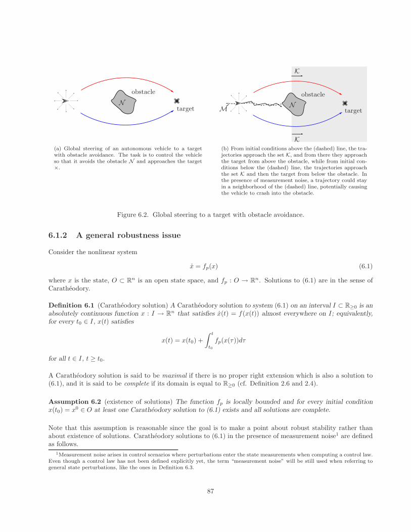
Ntarget

obstacle

(a) Global steering of an autonomous vehicle to a targetwith obstacle avoidance. The task is to control the vehicleso that it avoids the obstacle N and approaches the target×.

NM

K

K

target

obstacle

(b) From initial conditions above the (dashed) line, the tra-jectories approach the set K, and from there they approachthe target from above the obstacle, while from initial con-ditions below the (dashed) line, the trajectories approachthe set K and then the target from below the obstacle. Inthe presence of measurement noise, a trajectory could stayin a neighborhood of the (dashed) line, potentially causingthe vehicle to crash into the obstacle.

Figure 6.2. Global steering to a target with obstacle avoidance.

6.1.2 A general robustness issue

Consider the nonlinear system

x = fp(x) (6.1)

where x is the state, O ⊂ Rn is an open state space, and fp : O → R

n. Solutions to (6.1) are in the sense ofCaratheodory.

Definition 6.1 (Caratheodory solution) A Caratheodory solution to system (6.1) on an interval I ⊂ R≥0 is anabsolutely continuous function x : I → R

n that satisfies x(t) = f(x(t)) almost everywhere on I; equivalently,for every t0 ∈ I, x(t) satisfies

x(t) = x(t0) +

∫ t

t0

fp(x(τ))dτ

for all t ∈ I, t ≥ t0.

A Caratheodory solution is said to be maximal if there is no proper right extension which is also a solution to(6.1), and it is said to be complete if its domain is equal to R≥0 (cf. Definition 2.6 and 2.4).

Assumption 6.2 (existence of solutions) The function fp is locally bounded and for every initial conditionx(t0) = x0 ∈ O at least one Caratheodory solution to (6.1) exists and all solutions are complete.

Note that this assumption is reasonable since the goal is to make a point about robust stability rather thanabout existence of solutions. Caratheodory solutions to (6.1) in the presence of measurement noise1 are definedas follows.

1Measurement noise arises in control scenarios where perturbations enter the state measurements when computing a control law.Even though a control law has not been defined explicitly yet, the term “measurement noise” will be still used when referring togeneral state perturbations, like the ones in Definition 6.3.

87

Definition 6.3 (Caratheodory solutions with measurement noise) Given an interval I ⊂ R≥0 and a measurablefunction e : I → R

n, a Caratheodory solution to the system x = fp(x + e) on I is an absolutely continuousfunction x : I → O that satisfies x(t) = fp(x(t) + e(t)) almost everywhere on I; equivalently, for every t0 ∈ I,x(t) satisfies

x(t) = x(t0) +

∫ t

t0

fp(x(τ) + e(τ))dτ

for all t ∈ I.

A general result about vulnerability to measurement noise for a class of nonlinear systems is stated below.Let B ⊂ O be open and let Mi ⊂ O, i ∈ 1, . . . ,m, m ∈ N≥2, be disjoint sets satisfying

⋃mi=1 Mi = B. Let

M :=⋃

i,j∈1,...,m,i6=j

Mi ∩Mj .

Assumption 6.4 (state partition) Suppose that there exists T > 0 such that for each x ∈ M and each ρ > 0,there exist points zi, zj ∈ x+ ρB, i, j ∈ 1, . . . ,m, i 6= j, for which there exist Caratheodory solutions xi andxj to system (6.1) starting from zi and zj , respectively, satisfying xi(t) ∈ Mi \M and xj(t) ∈ Mj \M for allt ∈ [0, T ].

Theorem 6.5 (nonrobustness to measurement noise) Let Assumptions 6.2 and 6.4 hold. For every positiveconstants ε, ρ′, and ρ′′, and every x0 ∈ M+εB such that x0 +ρ′B ⊂ O and x0 +ρ′′B ⊂ B there exist a piecewiseconstant function e : dom e → εB and a maximal Caratheodory solution x : domx → O to x = fp(x + e)with x(0) = x0 such that x(t) ∈ (M + εB) ∩ B ∩ (x0 + ρ′B) for all t ∈ [0, T ′) for some T ′ ∈ (T ∗,∞], where

domx = dom e, T ∗ = minρ′,ρ′′m , and m := sup

1 + |f(η)|

∣∣ η ∈ x0 + maxρ′, ρ′′B. If T ′ is finite, then

limt→T ′ x(t) 6∈ B ∪ (x0 + ρ′B).

Theorem 6.5 states that for nonlinear systems with the topological properties in Assumption 6.4, thereexists a set of points of the state space (the set M) such that from every point x0 arbitrarily close to it, thereexists an arbitrarily small noise signal e and a solution x to x = fp(x+e) starting from x0 that stays close to anarbitrarily small neighborhood of M (intersected with a ball around x0). Moreover, if the solution ever leavessuch set then either it does it through the boundary of B or through the boundary of x0 + ρ′B.

Note that Assumption 6.4 states in general the scenario that arises, for example, in the stabilization problemsin Section 6.1.1. For the problem of stabilizing a disconnected set of points, the regions on each side of the linedefine the sets M1 and M2, respectively. Note that by global asymptotic stability, the union of M1 and M2

covers the state space. Then, the open set B is equal to O = Rn. The set M is given by M := M1 ∩M2 as

depicted in Figure 6.3(a) (it corresponds to the dashed line in Figure 6.1(b)). For the obstacle avoidance problemin Section 6.1.1, the state space is given by O = R

n \ N where N is a closed subset of Rn. The set of points

from which at least one trajectory converges to K by crossing into the set K from below the obstacle defines theset M1 while the set of points from above the obstacle define the set M2. By “global” convergence, M1 ∪M2

covers every point of the state space except the obstacle N and the set K. By stability and attractivity, thosesets are nonempty. Then, the set M is defined as the intersection of the closures of the sets M1 and M2. Theset B is given by the union of the sets Mi, i = 1, 2, and K is such that O = B ∪ K. Figure 6.3(b) depicts thesesets.

Under further assumptions, a version of Theorem 6.5 also holds in the state feedback case, that is, fornonlinear systems of the form

x = f(x, κ(x)) (6.2)

where x is the state, O ⊂ Rn is the open state space, κ : O → R

m, and f : O × Rm → R

n.

88

replacemen

A1

A2

M1M2

M

(a) Sets for the problem of globally steering an au-tonomous vehicle to different locations.

N

K

K

M1

M2

Mtarget

obstacle

(b) Sets for the problem of globally steering an au-tonomous vehicle to a target with obstacle avoidance.

Figure 6.3. Sets for the problems in Section 6.1.1.

Assumption 6.6 (regularity conditions for state feedback case) The function f is locally Lipschitz continuousin the first argument, locally uniformly in the second argument2; the function κ is locally bounded; and forevery x0 ∈ O at least one Caratheodory solution to (6.2) exists and all solutions from O are complete.

The function κ usually corresponds to a static control law designed to accomplish some control task. In thisscenario, a Caratheodory solution to (6.2) with measurement noise is as in Definition 6.3 but with measurementnoise entering through κ only, that is, x(t) satisfies

x(t) = x(t0) +

∫ t

t0

fp(x(τ), κ(x(τ) + e(τ)))dτ .

In this way, κ models the case of closed-loop systems where not every state component is perturbed by mea-surement noise because some of its components come from the natural dynamics. The assumption on f inAssumption 6.6 holds in many cases since the nonlinearities of the natural dynamics are Lipschitz continuous.For example, in the problem of regulating a double integrator to two different points of zero velocity by meansof state feedback, measurement noise does not enter the natural dynamics of the system (note that the naturaldynamics are linear in this case); it only enters through the feedback law.

Under Assumption 6.4, it follows that measurement noise entering the system through κ may prevent thetrajectories to approach the set A. This is stated in the next corollary.

Corollary 6.7 (state feedback case of general nonrobustness) Let Assumptions 6.4 and 6.6 hold. For everyε > 0 and every z ∈ M∩B there exists δ > 0 such that for each x0 ∈ (z+δB)∩B there exist a measurable functione : dom e → εB and a maximal Caratheodory solution x : domx → O to x = fp(x, κ(x + e)) with x(0) = x0

such that x(t) ∈ (M + εB) ∩ B for all t ∈ [0, T ′) for some T ′ ∈ (0,∞]. If T ′ is finite, then limt→T ′ x(t) 6∈ B.

As in Theorem 6.5, Corollary 6.7 states that under the stated assumptions, solutions can stay arbitrarily close tothe set M under the presence of arbitrarily small measurement noise. The proof of this result uses the fact thatTheorem 6.5 implies the existence of a maximal Krasovskii solution to (6.1) that stays in M (cf. [31, Proposition1.4]). Then, a solution and measurement noise signal for (6.2) is constructed to “track” the Krasovskii solutionwith arbitrary precision.

2A function h : O×Rm → R

n is continuous (locally Lipschitz continuous) in the first argument, locally uniformly in the secondargument if for each z ∈ O, each compact U ⊂ Rm, and each ε > 0 there exists δ > 0 (K > 0) such that |x − z| < δ implies|h(x, u) − h(z, u)| < ε (x, y ∈ (z + εB) ∩O implies |h(x, u) − h(y, u)| ≤ K|x− y|) for all u ∈ U .

89

6.1.3 Control design and analysis

In this section, nonlinear control systems of the following form are considered:

x = fp(x, u) (6.3)

where x is the state, O ⊂ Rn is an open state space, u ∈ R

m is the control input, and fp : O × Rm → R

n.

Assumption 6.8 (regularity of fp) The function fp is continuous.

Let A ⊂ O be a compact set. A hybrid controller, denoted by Hc, that renders the set A asymptoticallystable for (6.3) is designed. This hybrid controller confers to the closed-loop system a margin of robustness tonoise in the measurements of the state x. The proposed controller prevents the closed-loop system from beingvulnerable to measurement noise in scenarios like the ones discussed in the previous sections.

Hybrid controller

The hybrid controller Hc measures the output y := x+ e of (6.3), has logic (or discrete) state q that takesvalue in the finite set Q := 1, 2, . . . ,m, m ∈ N, has continuous dynamics

q = 0 (y, q) ∈ Cc ,

discrete dynamics

q+ ∈ Qc(y, q) (y, q) ∈ Dc ,

and output

u = κ(y, q) ,

where Cc, Dc are subsets of O × Q, Qc : O × Q →→ Q is a set-valued map that defines the update law for thediscrete state q, and κ is a function that defines the control law applied to (6.3).

Assume there exists a family of open sets Oq ⊂ Rn such that O := ∪q∈QOq and A ⊂ O. Suppose that

there exist functions Vq : O → [0,∞] that are C1 on Oq, for every z ∈ O \Oq are such that Vq(z) = ∞, and as|x| → ∞ or x→ ∂Oq are such that Vq(x) → ∞; a family of C0 functions κq : Oq → R

m; functions α1, α2 ∈ K∞;a continuous, positive-definite function ρ : R≥0 → R≥0; and a proper indicator3 ω of A on O such that

α1(ω(x)) ≤ minp∈Q

Vp(x) ≤ α2(ω(x)) ∀x ∈ O , (6.4)

and, for each q ∈ Q,〈∇Vq(x), fp(x, κq(x))〉 ≤ −ρ(Vq(x)) ∀x ∈ Oq . (6.5)

In some control problems, like in the regulation to a disconnected set of points (see Section 6.1.1), for eachq ∈ Q, there exist a proper indicator ωq of A on Oq and functions αq

1, αq2 ∈ K∞ satisfying

αq1(ωq(x)) ≤ Vq(x) ≤ αq

2(ωq(x)) ∀x ∈ Oq . (6.6)

The function ω : O → R≥0 constructed as ω(x) := minq∈Q s.t. x∈Oqωq(x) for each x ∈ O is a proper indicator

of A on O and the functions α1, α2 ∈ K∞ given by α1(s) := minp∈Q αp1(s), α2(s) := maxp∈Q α

p2(s) for each

s ∈ R≥0 satisfy (6.4).

3A function ω : U → R≥0 is a proper indicator of a compact set A ⊂ U with respect to an open set U if it is continuous, positivedefinite with respect to A, and such that ω(x) → ∞ as x→ ∂U (boundary of U) or |x| → ∞.

90

Assumption 6.9 (Vq condition on A ×Q) There exists γ > 0 such that (x, q) ∈ A ×Q and Vq(x) > 0 implyVq(x) > γ.

Assumption 6.9 is automatically satisfied when, for each q ∈ Q, Vq is positive definite with respect to Asince, in this case, it is impossible to have (x, q) ∈ A ×Q and Vq(x) > 0. In scenarios where Vq is non-zero ona subset of A, for example when A is a disconnected set like in Section 6.1.1, then the constant γ consists of auniform lower bound on Vq(x) on that subset.

Define constants µ > 1 and λ ∈ (0, µ − 1). Let γ > 0 be given by Assumption 6.9. The hybrid controllerHc defines the feedback law

u = κ(y, q) := κq(y)

when (y, q) ∈ Cc := Cac ∪ Cb

c , where

Cac :=

(x′, q′) ∈ O ×Q

∣∣∣∣ Vq′ (x′) ≤ µminp∈Q

Vp(x′)

(6.7)

Cbc := (x′, q′) ∈ O ×Q | Vq′(x′) ≤ γ , (6.8)

and has discrete dynamics given by

q+ ∈ Qc(y, q) := q′ ∈ Q | Vq(y) ≥ (µ− λ)Vq′ (y)

when (y, q) ∈ Dc, where Dc is given by

(x′, q′) ∈ O ×Q

∣∣∣∣ Vq′(x′) ≥ (µ− λ)minp∈Q

Vp(x′)

. (6.9)

The design parameters of the controller are µ and λ.

The basic idea in this construction is as follows. The discrete mode q selects the control law that is tobe applied to system (6.3). A change in the mode occurs only if the Lyapunov function for the current mode,Vq, gets larger or equal than the Lyapunov function for some other mode, say Vq′ , multiplied by µ − λ > 1.Points (x, q) ∈ O×Q with this property define the set Dc. Then, jumps are only allowed to modes that, at thecurrent state, have a Lyapunov function 1

(µ−λ) < 1 times smaller than the Lyapunov function at the current

mode. Flows are allowed when the Lyapunov function for the current mode is smaller or equal than µ timesthe minimum of the Lyapunov functions for the other modes. Then, with (6.5), the Lyapunov function for thecurrent mode is decreasing along solutions. Global asymptotic stability of the compact set A is achieved in thisway. This stability property and its robustness to external state perturbations is addressed in the next section.

Closed-loop system properties

From the construction of Hc, the nominal closed-loop hybrid system, denoted Hcl, can be written as

x = fp(x, κ(x, q))q = 0

(x, q) ∈ Cc (6.10)

x+ = xq+ ∈ Qc(x, q)

(x, q) ∈ Dc . (6.11)

With the regularity properties of fp, Vq, and κq on Oq for each q ∈ Q and the construction of the flow and

jump sets in (6.7)-(6.8) and (6.9), respectively, the resulting data (O, F, C,G,D) of the hybrid system Hcl with

91

state ξ := [xT qT ] given by

O := O × R, F (ξ) :=

[fp(x, κ(x, q))

0

], G(ξ) :=

[x

Qc(x, q)

], C := Cc, D := Dc

satisfies the hybrid basic conditions. Recall that these conditions guarantee, among other things, that hybridsystems have several structural properties, including the property that the limit of a sequence of solutions tohybrid systems is itself a solution.

Lemma 6.10 (hybrid basic conditions) Under Assumption 6.8 and 6.8, for every γ > 0 the closed-loop systemHcl satisfies the hybrid basic conditions. Moreover, Cc ⊂ ∪q∈QOq × q and Cc ∪Dc = O ×Q.

Proof. By definition, Cc ⊂ O ×Q ⊂ O. By continuity of Vq for each q ∈ Q, C = C. Then

C ∩ O = C ∩ (O × R) = C .

Then, C is relatively closed in O. Proceeding similarly, Dc ⊂ O × Q and it can be shown that D is relativelyclosed in O.

By definition of Cc, if (x, q) ∈ Cc then Vq(x) < ∞, and since by Assumption 6.8 this holds only if (x, q) ∈Oq × q, then Cc ⊂ ∪q∈Q(Oq × q). Every point in (∪q∈Q(Oq × q)) \ Ca

c satisfies, in particular, Vq(x) >µminp∈Q Vp(x). By definition of Dc, every such point is in Dc. Moreover, every point (x, q) ∈ (O × Q) \(∪q∈Q(Oq × q)) is such that Vq(x) = ∞. By definition of O, for each such point there exists q′ ∈ Q such thatVq′ (x) <∞. Then, every such point is in Dc. This establishes that Cc ∪Dc = O ×Q.

Since for each q ∈ Q, κ(x, q) = κq(x) for each x ∈ Oq and κq, fp are continuous, F is continuous on itsdomain of definition and nonempty for each point in ∪q∈Q(Oq × q), in particular, for each point in Cc.

By construction of Dc and Qc, Qc(x, q) 6= ∅ and Qc(x, q) ⊂ Cc for every (x, q) ∈ Dc. For every (x, q) ∈ Dc

and every sequence xi, qi such that (xi, qi) ∈ Dc and xi → x, qi → q it holds that

Vqi(xi) ≥ (µ− λ)Vpi

(xi) (6.12)

where pi ∈ Qc(xi, qi). For qi and pi to converge, pi = p and qi = q for large enough i, for some p, q ∈ Q. Takinglimit at each side of (6.12) and using the continuity properties of Vq for each q ∈ Q yields

Vq(x) ≥ (µ− λ)Vp(x) . (6.13)

Then, p ∈ Qc(x, q) and Qc is outer semicontinuous in its domain of definition.

As discussed in the previous section, the construction of the hybrid controller is such that the logic modeq is updated so that the Lyapunov function for the closed-loop hybrid system Hcl given by W (x, q) := Vq(x)decreases along solutions. This leads to the following “global” asymptotic stability result of the compact setA×Q.

Theorem 6.11 (nominal asymptotic stability of A) Under Assumptions 6.8 and 6.9, the compact set A×Q isasymptotically stable with basin of attraction BA = O ×Q for the hybrid system Hcl.

In the case that noise e corrupts the measurement of the state x, that is, the controller measures the outputy = x+ e, statements about robustness of the above asymptotic stability property can be made by perturbationanalysis. Roughly speaking, the main idea is to model the measurement noise as a state perturbation of sizeδ∗ > 0 and replace the instances in (6.10) and (6.11) where the controller measures the state by the state

92

perturbation x+ δ∗B (these places are the first argument of κ, Cc, Qc, and Dc). Then, the resulting perturbedhybrid system will have the original data (O, F, C,G,D) perturbed and, by construction, satisfying certainconditions that guarantee that the stability property is semiglobally and practically preserved. The followingresult uses this technique to show that A × Q is semiglobally practically asymptotically stable under smallenough measurement noise.

Theorem 6.12 (robustness of Hcl to measurement noise) For given parameters µ > 1 and λ ∈ (0, µ− 1) of thecontroller Hc, there exists β ∈ KLL and for each ε > 0 and each compact set K ⊂ O there exists δ∗ > 0, suchthat for each admissible measurement noise e : dom e → δB with δ ∈ [0, δ∗], solutions (x, q) to Hcl exist, arecomplete, and for initial conditions (x0, q0) ∈ K ×Q satisfy

ω(x(t, j)) ≤ β(ω(x0), t, j) + ε ∀(t, j) ∈ dom(x, q) .

Theorem 6.12 guarantees that for each compact set of initial conditions, the closed-loop system Hcl toleratesa nonzero level δ∗ > 0 of measurement noise. This corresponds to the margin of robustness that the hybridcontrol strategy confers to the closed-loop system. This margin of robustness to measurement noise overcomesthe issues described in the control problems in Section 6.1.1.

An estimate of this margin of robustness can be computed from the sets Cc and Dc. Figure 6.4 shows thesesets, along with level sets of the Lyapunov functions, for the problem of globally stabilizing a disconnected set ofpoints in Section 6.1.1. Given points A1,A2 with associated Lyapunov functions V1, V2 and control laws κ1, κ2

satisfying the conditions in Section 6.1.3, respectively, and parameters µ > 1, λ ∈ (0, µ− 1), the set Cc and Dc

can be written as

Cc := (Cc1 × 1) ∪ (Cc2 × 2), Dc := (Dc1 × 1) ∪ (Dc2 × 2) (6.14)

where Cc1, Cc2, Dc1, Dc2 ⊂ O. Figure 6.4 depicts these sets and a solution to Hcl. The solution, which startsfrom a point in the flow set with q = 1, experiences a jump when in the jump set that maps q to 2. Fromthere, the solution flows with q = 2 until, once in the jump set again, a jump maps q to 1. From there on, thesolution stays in the flow set with mode q = 1 and approaches A1. From this discussion, it follows that underthe presence of measurement noise, for the closed-loop system to experience the nonrobust behavior discussedin Section 6.1.1, the size of the measurement noise needs to be so that fast switching between the modes occurs.This is only possible from certain points of the state space if the measurement noise is larger that the minimumdistance between the sets Dc1 and Dc2. Then, this analysis suggests that the maximum measurement noise forwhich solutions approach the target set without experiencing the phenomenon described in Theorem 6.5 andCorollary 6.7 is given by

δ1 := minz1∈Dc1z2∈Dc2

|z1 − z2| . (6.15)

This level depends proportionally on µ, and therefore, can be tuned by varying this control parameter. Forthe setting in Figure 6.4, as µ increases, the set Dc1 (Dc2) becomes smaller and centered around the set A2

(A1). Clearly, the maximum margin of robustness to measurement noise that can be obtained with this controlstrategy is upper bounded by the distance between A1 and A2.

As discussed in Section 3.3, measurement noise in hybrid systems can lead to nonexistence of solutions,even when the measurement noise is arbitrarily small. The overlap between the set Cc and Dc obtained fromusing µ in the definition of Cc and µ−λ in the definition of Dc guarantees such existence for measurement noisesmaller than the minimum overlap given by

δ2 := minδ21, δ22, δ21 := minz1∈O\Dc1,z2∈O\Cc1

|z1 − z2|,

δ22 := minz1∈O\Dc2,z2∈O\Cc2

|z1 − z2| ,

93

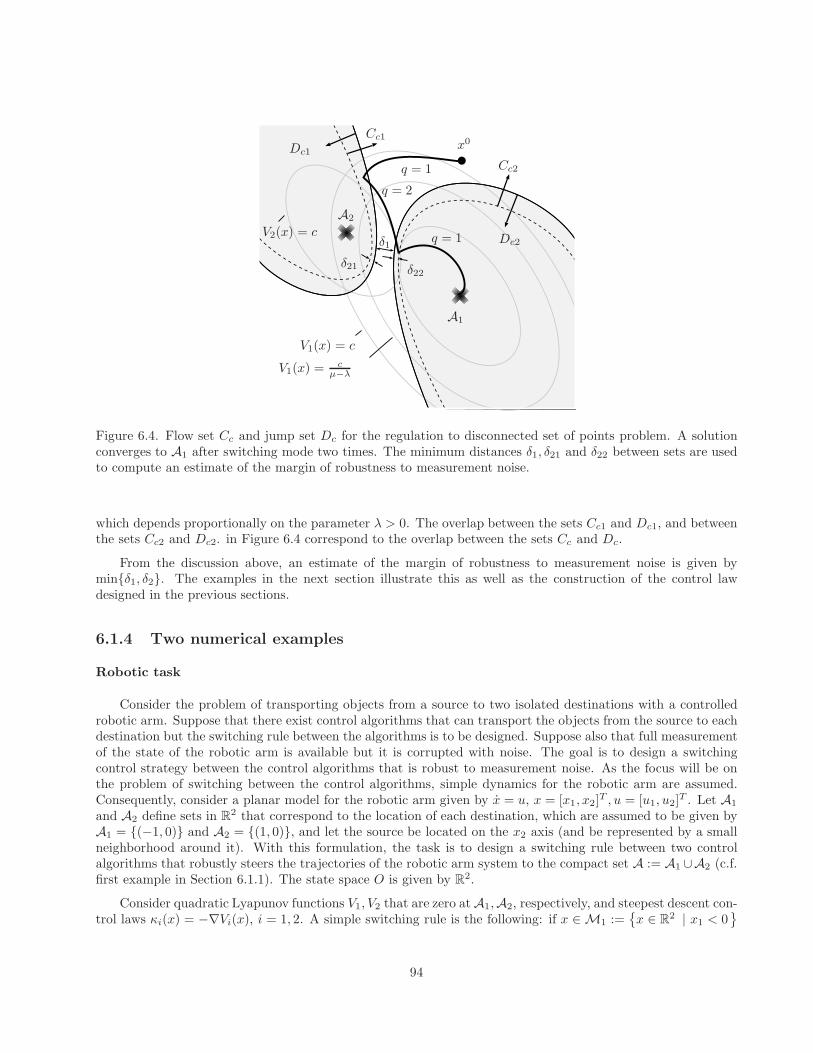
A1

A2

x0

q = 2

q = 1

q = 1

δ1

δ21 δ22

Dc1

Dc2

Cc1

Cc2

V1(x) = c

V2(x) = c

V1(x) = cµ−λ

Figure 6.4. Flow set Cc and jump set Dc for the regulation to disconnected set of points problem. A solutionconverges to A1 after switching mode two times. The minimum distances δ1, δ21 and δ22 between sets are usedto compute an estimate of the margin of robustness to measurement noise.

which depends proportionally on the parameter λ > 0. The overlap between the sets Cc1 and Dc1, and betweenthe sets Cc2 and Dc2. in Figure 6.4 correspond to the overlap between the sets Cc and Dc.

From the discussion above, an estimate of the margin of robustness to measurement noise is given byminδ1, δ2. The examples in the next section illustrate this as well as the construction of the control lawdesigned in the previous sections.

6.1.4 Two numerical examples

Robotic task

Consider the problem of transporting objects from a source to two isolated destinations with a controlledrobotic arm. Suppose that there exist control algorithms that can transport the objects from the source to eachdestination but the switching rule between the algorithms is to be designed. Suppose also that full measurementof the state of the robotic arm is available but it is corrupted with noise. The goal is to design a switchingcontrol strategy between the control algorithms that is robust to measurement noise. As the focus will be onthe problem of switching between the control algorithms, simple dynamics for the robotic arm are assumed.Consequently, consider a planar model for the robotic arm given by x = u, x = [x1, x2]

T , u = [u1, u2]T . Let A1

and A2 define sets in R2 that correspond to the location of each destination, which are assumed to be given by

A1 = (−1, 0) and A2 = (1, 0), and let the source be located on the x2 axis (and be represented by a smallneighborhood around it). With this formulation, the task is to design a switching rule between two controlalgorithms that robustly steers the trajectories of the robotic arm system to the compact set A := A1 ∪A2 (c.f.first example in Section 6.1.1). The state space O is given by R

2.

Consider quadratic Lyapunov functions V1, V2 that are zero at A1,A2, respectively, and steepest descent con-trol laws κi(x) = −∇Vi(x), i = 1, 2. A simple switching rule is the following: if x ∈ M1 :=

x ∈ R

2 | x1 < 0

94

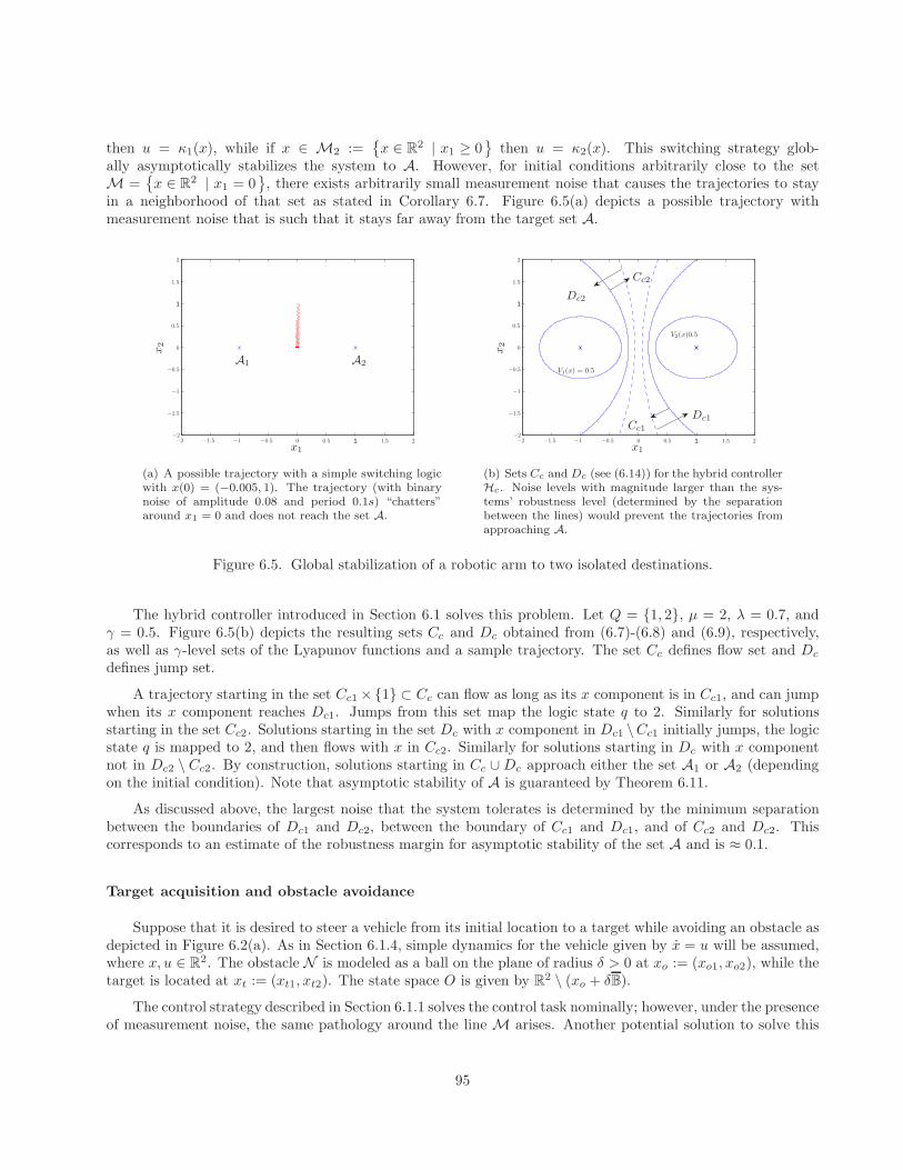
then u = κ1(x), while if x ∈ M2 :=x ∈ R

2 | x1 ≥ 0

then u = κ2(x). This switching strategy glob-ally asymptotically stabilizes the system to A. However, for initial conditions arbitrarily close to the setM =

x ∈ R

2 | x1 = 0, there exists arbitrarily small measurement noise that causes the trajectories to stay

in a neighborhood of that set as stated in Corollary 6.7. Figure 6.5(a) depicts a possible trajectory withmeasurement noise that is such that it stays far away from the target set A.

1

1

A1 A2

x1

x2

2

2

1.5

1.5

0.5

0.5

0

0

−0.5

−0.5

−1

−1

−1.5

−1.5−2−2

(a) A possible trajectory with a simple switching logicwith x(0) = (−0.005, 1). The trajectory (with binarynoise of amplitude 0.08 and period 0.1s) “chatters”around x1 = 0 and does not reach the set A.

1

1

Dc1

Dc2

Cc1

Cc2

V1(x) = 0.5

V2(x)0.5

x1

x2

2

2

1.5

1.5

0.5

0.5

0

0

−0.5

−0.5

−1

−1

−1.5

−1.5−2−2

(b) Sets Cc and Dc (see (6.14)) for the hybrid controllerHc. Noise levels with magnitude larger than the sys-tems’ robustness level (determined by the separationbetween the lines) would prevent the trajectories fromapproaching A.

Figure 6.5. Global stabilization of a robotic arm to two isolated destinations.

The hybrid controller introduced in Section 6.1 solves this problem. Let Q = 1, 2, µ = 2, λ = 0.7, andγ = 0.5. Figure 6.5(b) depicts the resulting sets Cc and Dc obtained from (6.7)-(6.8) and (6.9), respectively,as well as γ-level sets of the Lyapunov functions and a sample trajectory. The set Cc defines flow set and Dc

defines jump set.

A trajectory starting in the set Cc1 ×1 ⊂ Cc can flow as long as its x component is in Cc1, and can jumpwhen its x component reaches Dc1. Jumps from this set map the logic state q to 2. Similarly for solutionsstarting in the set Cc2. Solutions starting in the set Dc with x component in Dc1 \Cc1 initially jumps, the logicstate q is mapped to 2, and then flows with x in Cc2. Similarly for solutions starting in Dc with x componentnot in Dc2 \ Cc2. By construction, solutions starting in Cc ∪ Dc approach either the set A1 or A2 (dependingon the initial condition). Note that asymptotic stability of A is guaranteed by Theorem 6.11.

As discussed above, the largest noise that the system tolerates is determined by the minimum separationbetween the boundaries of Dc1 and Dc2, between the boundary of Cc1 and Dc1, and of Cc2 and Dc2. Thiscorresponds to an estimate of the robustness margin for asymptotic stability of the set A and is ≈ 0.1.

Target acquisition and obstacle avoidance

Suppose that it is desired to steer a vehicle from its initial location to a target while avoiding an obstacle asdepicted in Figure 6.2(a). As in Section 6.1.4, simple dynamics for the vehicle given by x = u will be assumed,where x, u ∈ R

2. The obstacle N is modeled as a ball on the plane of radius δ > 0 at xo := (xo1, xo2), while thetarget is located at xt := (xt1, xt2). The state space O is given by R

2 \ (xo + δB).

The control strategy described in Section 6.1.1 solves the control task nominally; however, under the presenceof measurement noise, the same pathology around the line M arises. Another potential solution to solve this

95

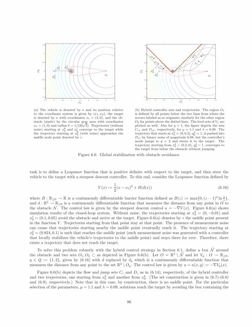
x10

x00

x20

C

x1

x2

3.532.52

1.5

1.5

0.5

0.5

0

0

−0.5

−0.5

−1

1

1

−1.5

xt

(a) The vehicle is denoted by ⊲ and its position relativeto the coordinate system is given by (x1, x2), the targetis denoted by x with coordinates xt = (3, 0), and the ob-stacle (static) by the circular gray area with coordinatesxo = (1, 0) and radius δ = 1/(20

√2). Trajectories (without

noise) starting at x00 and x1

0 converge to the target whilethe trajectory starting at x2

0 (with noise) approaches thesaddle node point denoted by .

x30x4

0

O1O1

Dc1 Dc1

Cc1

Cc1

x1

x2

3.532.52

1.5

1.5

0.5

0.5

0

0

−0.5

−0.5

−1

1

1

−1.5

xt

(b) Hybrid controller sets and trajectories. The region O1

is defined by all points below the two lines from where thearrows labeled as so originate; similarly for the other regionO2 for points above the dotted lines. The level sets of V1 areplotted as well. Also for q = 1, the figure depicts the setsCc1 and Dc1, respectively, for µ = 1.1 and λ = 0.09. Thetrajectory that starts at x3

0 = (0, 0.2), q30 = 1, is pushed intoDc1 by binary noise of magnitude 0.08, but the controller’smode jumps to q = 2 and steers it to the target. Thetrajectory starting from x4

0= (0.2, 0), q4

0= 1, converges to

the target from below the obstacle without jumping.

Figure 6.6. Global stabilization with obstacle avoidance.

task is to define a Lyapunov function that is positive definite with respect to the target, and then steer thevehicle to the target with a steepest descent controller. To this end, consider the Lyapunov function defined by

V (x) :=1

2(x− xt)

2 +B(d(x)) (6.16)

where B : R≥0 → R is a continuously differentiable barrier function defined as B(z) := max0, (z − 1)2 ln 1z,

and d : R2 → R≥0 is a continuously differentiable function that measures the distance from any point in O to

the obstacle N . The control law is given by the steepest descent control u = −∇V (x). Figure 6.6(a) showssimulation results of the closed-loop system. Without noise, the trajectories starting at x0

0 = (0,−0.01) andx1

0 = (0.1, 0.05) avoid the obstacle and arrive at the target. Figure 6.6(a) denotes by the saddle point presentin the function V . Trajectories starting from that point stay at that point. The presence of measurement noisecan cause that trajectories starting nearby the saddle point eventually reach it. The trajectory starting atx2

0 = (0.824, 0.1) is such that reaches the saddle point (such measurement noise was generated with a controllerthat locally stabilizes the vehicle’s trajectories to the saddle point) and stays there for ever. Therefore, thereexists a trajectory that does not reach the target.

To solve this problem robustly with the hybrid control strategy in Section 6.1, define a box N aroundthe obstacle and two sets O1, O2 ⊂ as depicted in Figure 6.6(b). Let O = R

2 \ N and let Vq : O → R≥0,q ∈ Q := 1, 2, given by (6.16) with d replaced by dq which is a continuously differentiable function thatmeasures the distance from any point to the set R

2 \Oq. The control law is given by u = κ(x, q) := −∇Vq(x).

Figure 6.6(b) depicts the flow and jump sets Cc and Dc as in (6.14), respectively, of the hybrid controllerand two trajectories, one starting from x3

0 and another from x40. (The set construction is given in (6.7)-(6.8)

and (6.9), respectively.) Note that in this case, by construction, there is no saddle point. For the particularselection of the parameters, µ = 1.1 and λ = 0.09, solutions reach the target by avoiding the box containing the

96

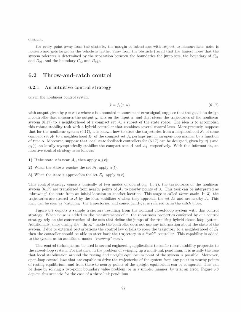
obstacle.

For every point away from the obstacle, the margin of robustness with respect to measurement noise isnonzero and gets larger as the vehicle is farther away from the obstacle (recall that the largest noise that thesystem tolerates is determined by the separation between the boundaries the jump sets, the boundary of Cc1

and Dc1, and the boundary Cc2 and Dc2).

6.2 Throw-and-catch control

6.2.1 An intuitive control strategy

Given the nonlinear control system

x = fp(x, u) (6.17)

with output given by y = x+e where e is a bounded measurement error signal, suppose that the goal is to designa controller that measures the output y, acts on the input u, and that steers the trajectories of the nonlinearsystem (6.17) to a neighborhood of a compact set A, a subset of the state space. The idea is to accomplishthis robust stability task with a hybrid controller that combines several control laws. More precisely, supposethat for the nonlinear system (6.17), it is known how to steer the trajectories from a neighborhood S1 of somecompact set A1 to a neighborhood E1 of the compact set A, perhaps just in an open-loop manner by a functionof time α. Moreover, suppose that local state feedback controllers for (6.17) can be designed, given by κ(·) andκ1(·), to locally asymptotically stabilize the compact sets A and A1, respectively. With this information, anintuitive control strategy is as follows:

1) If the state x is near A1, then apply κ1(x);

2) When the state x reaches the set S1, apply α(t).

3) When the state x approaches the set E1, apply κ(x).

This control strategy consists basically of two modes of operation. In 2), the trajectories of the nonlinearsystem (6.17) are transferred from nearby points of A1 to nearby points of A. This task can be interpreted as“throwing” the state from an initial location to another location. This stage is called throw mode. In 3), thetrajectories are steered to A by the local stabilizer κ when they approach the set E1 and are nearby A. Thislogic can be seen as “catching” the trajectories, and consequently, it is referred to as the catch mode.

Figure 6.7 depicts a sample trajectory resulting from the nominal closed-loop system with this controlstrategy. When noise is added to the measurements of x, the robustness properties conferred by our controlstrategy rely on the construction of the sets that define the jumps of the resulting hybrid closed-loop system.Additionally, since during the “throw” mode the controller does not use any information about the state of thesystem, if due to external perturbations the control law α fails to steer the trajectory to a neighborhood of E1

then the controller should be able to steer back the trajectory to a “safe” controller. This capability is addedto the system as an additional mode: “recovery” mode.

This control technique can be used in several engineering applications to confer robust stability properties tothe closed-loop system. For instance, in the problem of swinging up a multi-link pendulum, it is usually the casethat local stabilization around the resting and upright equilibrium point of the system is possible. Moreover,open-loop control laws that are capable to drive the trajectories of the system from any point to nearby pointsof resting equilibrium, and from there to nearby points of the upright equilibrium can be computed. This canbe done by solving a two-point boundary value problem, or in a simpler manner, by trial an error. Figure 6.8depicts this scenario for the case of a three-link pendulum.

97

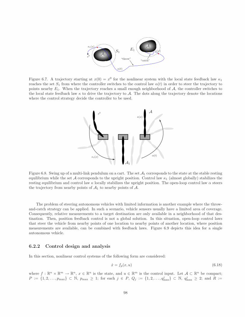
x0

κ1(x)

κ(x)

α(t)

A1

AS1

E1

“throw”“catch”

Figure 6.7. A trajectory starting at x(0) = x0 for the nonlinear system with the local state feedback law κ1

reaches the set S1 from where the controller switches to the control law α(t) in order to steer the trajectory topoints nearby E1. When the trajectory reaches a small enough neighborhood of A, the controller switches tothe local state feedback law κ to drive the trajectory to A. The dots along the trajectory denote the locationswhere the control strategy decide the controller to be used.

x0

κ1(x)

κ(x)

α(t)

A1

A

Figure 6.8. Swing up of a multi-link pendulum on a cart. The set A1 corresponds to the state at the stable restingequilibrium while the set A corresponds to the upright position. Control law κ1 (almost globally) stabilizes theresting equilibrium and control law κ locally stabilizes the upright position. The open-loop control law α steersthe trajectory from nearby points of A1 to nearby points of A.

The problem of steering autonomous vehicles with limited information is another example where the throw-and-catch strategy can be applied. In such a scenario, vehicle sensors usually have a limited area of coverage.Consequently, relative measurements to a target destination are only available in a neighborhood of that des-tination. Then, position feedback control is not a global solution. In this situation, open-loop control lawsthat steer the vehicle from nearby points of one location to nearby points of another location, where positionmeasurements are available, can be combined with feedback laws. Figure 6.9 depicts this idea for a singleautonomous vehicle.

6.2.2 Control design and analysis

In this section, nonlinear control systems of the following form are considered:

x = fp(x, u) (6.18)

where f : Rn × R

m → Rn, x ∈ R

n is the state, and u ∈ Rm is the control input. Let A ⊂ R

n be compact;P := 1, 2, . . . , pmax ⊂ N, pmax ≥ 1; for each j ∈ P , Qj := 1, 2, . . . , qj

max ⊂ N, qjmax ≥ 2; and R :=

98

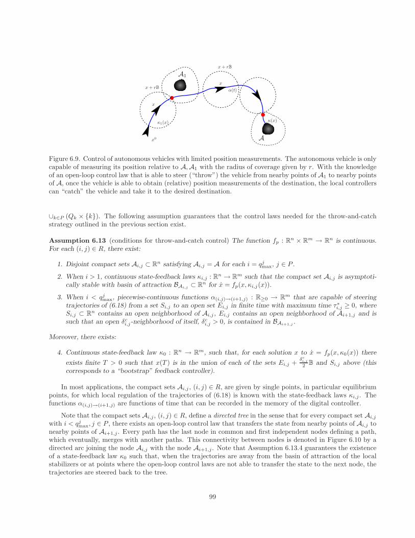
x0

κ1(x)κ(x)

α(t)

x

xx+ rB

x+ rB

A1

A

Figure 6.9. Control of autonomous vehicles with limited position measurements. The autonomous vehicle is onlycapable of measuring its position relative to A,A1 with the radius of coverage given by r. With the knowledgeof an open-loop control law that is able to steer (“throw”) the vehicle from nearby points of A1 to nearby pointsof A, once the vehicle is able to obtain (relative) position measurements of the destination, the local controllerscan “catch” the vehicle and take it to the desired destination.

∪k∈P (Qk × k). The following assumption guarantees that the control laws needed for the throw-and-catchstrategy outlined in the previous section exist.

Assumption 6.13 (conditions for throw-and-catch control) The function fp : Rn × R

m → Rn is continuous.

For each (i, j) ∈ R, there exist:

1. Disjoint compact sets Ai,j ⊂ Rn satisfying Ai,j = A for each i = qj

max, j ∈ P .

2. When i > 1, continuous state-feedback laws κi,j : Rn → R

m such that the compact set Ai,j is asymptoti-cally stable with basin of attraction BAi,j

⊂ Rn for x = fp(x, κi,j(x)).

3. When i < qjmax, piecewise-continuous functions α(i,j)→(i+1,j) : R≥0 → R

m that are capable of steeringtrajectories of (6.18) from a set Si,j to an open set Ei,j in finite time with maximum time τ∗i,j ≥ 0, whereSi,j ⊂ R

n contains an open neighborhood of Ai,j , Ei,j contains an open neighborhood of Ai+1,j and issuch that an open δc

i,j-neighborhood of itself, δci,j > 0, is contained in BAi+1,j

.

Moreover, there exists:

4. Continuous state-feedback law κ0 : Rn → R

m, such that, for each solution x to x = fp(x, κ0(x)) there

exists finite T > 0 such that x(T ) is in the union of each of the sets Ei,j +δc

i,j

2 B and Si,j above (thiscorresponds to a “bootstrap” feedback controller).

In most applications, the compact sets Ai,j , (i, j) ∈ R, are given by single points, in particular equilibriumpoints, for which local regulation of the trajectories of (6.18) is known with the state-feedback laws κi,j . Thefunctions α(i,j)→(i+1,j) are functions of time that can be recorded in the memory of the digital controller.

Note that the compact sets Ai,j , (i, j) ∈ R, define a directed tree in the sense that for every compact set Ai,j

with i < qjmax, j ∈ P , there exists an open-loop control law that transfers the state from nearby points of Ai,j to

nearby points of Ai+1,j . Every path has the last node in common and first independent nodes defining a path,which eventually, merges with another paths. This connectivity between nodes is denoted in Figure 6.10 by adirected arc joining the node Ai,j with the node Ai+1,j . Note that Assumption 6.13.4 guarantees the existenceof a state-feedback law κ0 such that, when the trajectories are away from the basin of attraction of the localstabilizers or at points where the open-loop control laws are not able to transfer the state to the next node, thetrajectories are steered back to the tree.

99

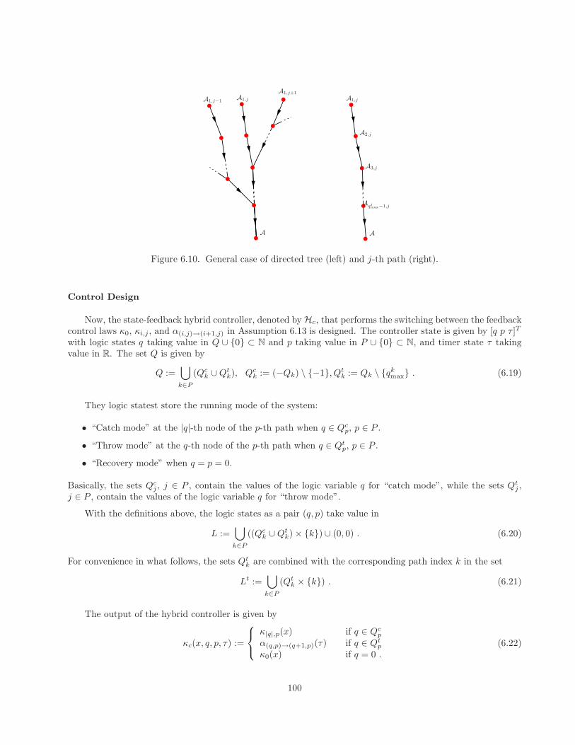
A1,j−1 A1,jA1,j

A2,j

A3,j

Aqjmax−1,j

A1,j+1

AA

Figure 6.10. General case of directed tree (left) and j-th path (right).

Control Design

Now, the state-feedback hybrid controller, denoted by Hc, that performs the switching between the feedbackcontrol laws κ0, κi,j , and α(i,j)→(i+1,j) in Assumption 6.13 is designed. The controller state is given by [q p τ ]T

with logic states q taking value in Q ∪ 0 ⊂ N and p taking value in P ∪ 0 ⊂ N, and timer state τ takingvalue in R. The set Q is given by

Q :=⋃

k∈P

(Qck ∪Qt

k), Qck := (−Qk) \ −1, Qt

k := Qk \ qkmax . (6.19)

They logic statest store the running mode of the system:

• “Catch mode” at the |q|-th node of the p-th path when q ∈ Qcp, p ∈ P .

• “Throw mode” at the q-th node of the p-th path when q ∈ Qtp, p ∈ P .

• “Recovery mode” when q = p = 0.

Basically, the sets Qcj, j ∈ P , contain the values of the logic variable q for “catch mode”, while the sets Qt

j ,j ∈ P , contain the values of the logic variable q for “throw mode”.

With the definitions above, the logic states as a pair (q, p) take value in

L :=⋃

k∈P

((Qck ∪Qt

k) × k) ∪ (0, 0) . (6.20)

For convenience in what follows, the sets Qtk are combined with the corresponding path index k in the set

Lt :=⋃

k∈P

(Qtk × k) . (6.21)

The output of the hybrid controller is given by

κc(x, q, p, τ) :=

κ|q|,p(x) if q ∈ Qcp

α(q,p)→(q+1,p)(τ) if q ∈ Qtp

κ0(x) if q = 0 .(6.22)

100

The following sets are part of the control logic.

I) Sets for “Catch mode” update logic

For each (i, j) ∈ Lt, let Ei,j and δci,j be given as in Assumption 6.13.3, and define

Dci,j = Ei,j + δc

i,jB, Cci,j = Rn \Dc

i,j +δci,j

2B .

II) Sets for “Throw mode” update logic

For each (i, j) ∈ Lt, let Si,j be given as in Assumption 6.13.3, and define Dti,j to be a closed set such that

for some δti,j > 0 satisfies

Ai,j + δti,jB ⊂ Dt

i,j , Dti,j +

δti,j

2B ⊂ Si,j .

Then, for each (i, j) ∈ Lt, let Cti,j be given by

Cti,j := Rn \Dt

i,j +δti,j

2B .

III) Sets for “Recovering mode” update logic

For each (i, j) ∈ ∪k∈P (Qck × k), for some δr

i,j > 0, define

Cri,j := reachi,j(D

c|i|−1,j) + δr

i,jB (6.23)

where reachi,j(Dc|i|−1,j) is the reachable set of x = fp(x, κ|i|,j(x)) from Dc

|i|−1,j. Also, define Dri,j as

Dri,j := Rn \ Cr

i,j +δri,j

2B . (6.24)

Define Cr0,0 and Dr

0,0 as follows. For each (i, j) ∈ ∪k∈P (Qk ×k) define an auxiliary set Dri,j to be a closed

set such that for some δri,j > 0 satisfies

Ai,j + δri,jB ⊂ Dr

i,j , Dri,j +

δri,j

2B ⊂ Dc

i−1,j ∪Dti,j ,

where Dc0,j = Dt

qjmax,j

= ∅ for all j ∈ P . Then, Cr0,0 and Dr

0,0 are given by

Dr0,0 :=

⋃

(i,j)∈∪k∈P (Qk×k)

Dri,j , Cr

0,0 := Rn \Dr0,0 +

δr0,0

2B

where δr0,0 is the minimum δr

i,j over ∪k∈P (Qk × k).With these definitions, the update laws are designed as follows. If in throw mode and the state x is such

that a “catch” is possible, i.e.

(q, p) ∈ Qtp × p, x ∈ Dc

q,p , (6.25)

then jumps to catch mode are enabled with update law q+ = −(|q| + 1). If in catch mode and the state x issuch that a “throw” is possible, i.e.

(q, p) ∈(Qc

p \ −qpmax

)× p, x ∈ Dt

|q|,p , (6.26)

101

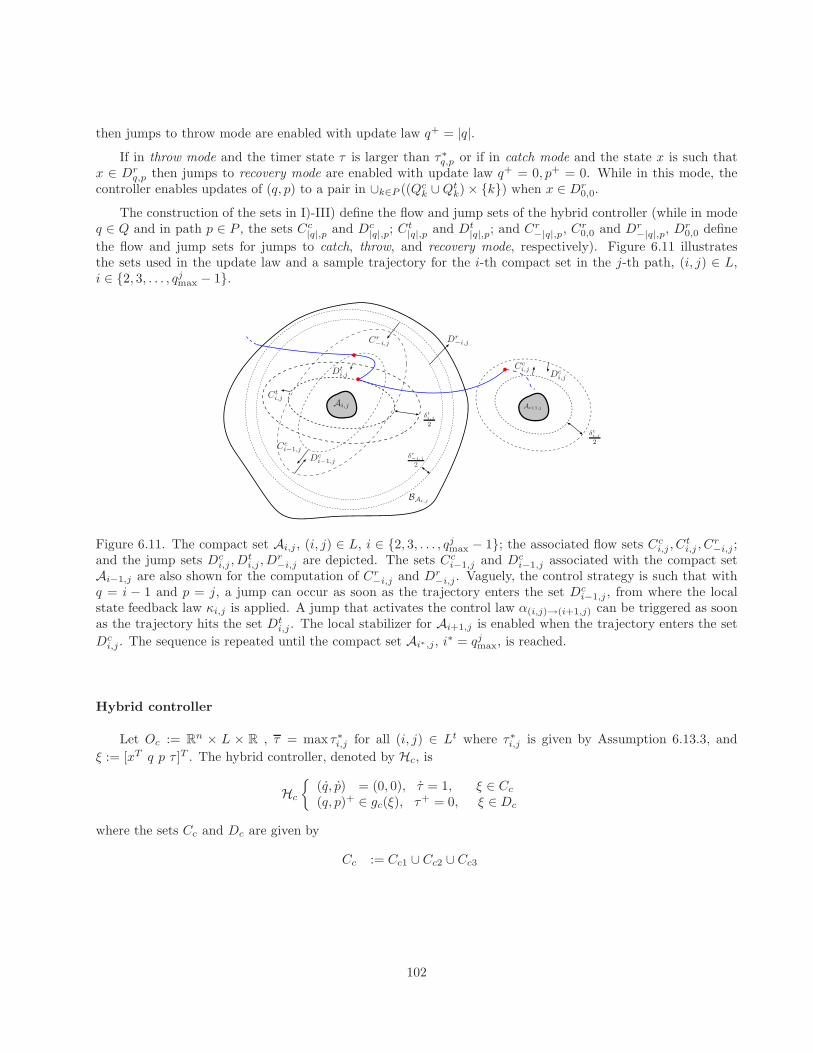
then jumps to throw mode are enabled with update law q+ = |q|.If in throw mode and the timer state τ is larger than τ∗q,p or if in catch mode and the state x is such that

x ∈ Drq,p then jumps to recovery mode are enabled with update law q+ = 0, p+ = 0. While in this mode, the

controller enables updates of (q, p) to a pair in ∪k∈P ((Qck ∪Qt

k) × k) when x ∈ Dr0,0.

The construction of the sets in I)-III) define the flow and jump sets of the hybrid controller (while in modeq ∈ Q and in path p ∈ P , the sets Cc

|q|,p and Dc|q|,p; C

t|q|,p and Dt

|q|,p; and Cr−|q|,p, C

r0,0 and Dr

−|q|,p, Dr0,0 define

the flow and jump sets for jumps to catch, throw, and recovery mode, respectively). Figure 6.11 illustratesthe sets used in the update law and a sample trajectory for the i-th compact set in the j-th path, (i, j) ∈ L,i ∈ 2, 3, . . . , qj

max − 1.

Ai,j Ai+1,j

BAi,j

Dci,j

Cci,jDt

i,j

Cti,j

Dci−1,j

Cci−1,j

Dr−i,jCr

−i,j

δci,j

2

δr−i,j

2

δti,j

2

Figure 6.11. The compact set Ai,j , (i, j) ∈ L, i ∈ 2, 3, . . . , qjmax − 1; the associated flow sets Cc

i,j , Cti,j , C

r−i,j ;

and the jump sets Dci,j , D

ti,j , D

r−i,j are depicted. The sets Cc

i−1,j and Dci−1,j associated with the compact set

Ai−1,j are also shown for the computation of Cr−i,j and Dr

−i,j . Vaguely, the control strategy is such that withq = i − 1 and p = j, a jump can occur as soon as the trajectory enters the set Dc

i−1,j , from where the localstate feedback law κi,j is applied. A jump that activates the control law α(i,j)→(i+1,j) can be triggered as soonas the trajectory hits the set Dt

i,j . The local stabilizer for Ai+1,j is enabled when the trajectory enters the set

Dci,j . The sequence is repeated until the compact set Ai∗,j, i

∗ = qjmax, is reached.

Hybrid controller

Let Oc := Rn × L × R , τ = max τ∗i,j for all (i, j) ∈ Lt where τ∗i,j is given by Assumption 6.13.3, and

ξ := [xT q p τ ]T . The hybrid controller, denoted by Hc, is

Hc

(q, p) = (0, 0), τ = 1, ξ ∈ Cc

(q, p)+ ∈ gc(ξ), τ+ = 0, ξ ∈ Dc

where the sets Cc and Dc are given by

Cc := Cc1 ∪ Cc2 ∪Cc3

102

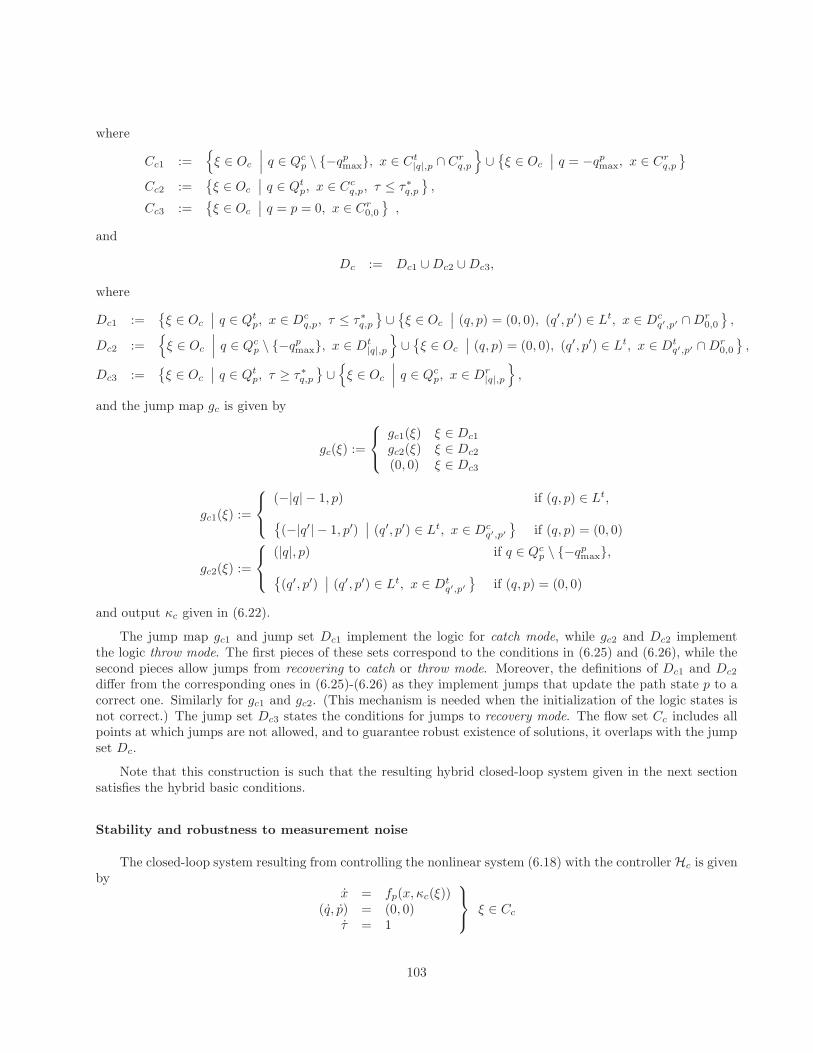
where

Cc1 :=ξ ∈ Oc

∣∣∣ q ∈ Qcp \ −qp

max, x ∈ Ct|q|,p ∩ Cr

q,p

∪

ξ ∈ Oc

∣∣ q = −qpmax, x ∈ Cr

q,p

Cc2 :=ξ ∈ Oc

∣∣ q ∈ Qtp, x ∈ Cc

q,p, τ ≤ τ∗q,p

,

Cc3 :=ξ ∈ Oc

∣∣ q = p = 0, x ∈ Cr0,0

,

and

Dc := Dc1 ∪Dc2 ∪Dc3,

where

Dc1 :=ξ ∈ Oc

∣∣ q ∈ Qtp, x ∈ Dc

q,p, τ ≤ τ∗q,p

∪

ξ ∈ Oc

∣∣ (q, p) = (0, 0), (q′, p′) ∈ Lt, x ∈ Dcq′,p′ ∩Dr

0,0

,

Dc2 :=ξ ∈ Oc

∣∣∣ q ∈ Qcp \ −qp

max, x ∈ Dt|q|,p

∪

ξ ∈ Oc

∣∣ (q, p) = (0, 0), (q′, p′) ∈ Lt, x ∈ Dtq′,p′ ∩Dr

0,0

,

Dc3 :=ξ ∈ Oc

∣∣ q ∈ Qtp, τ ≥ τ∗q,p

∪

ξ ∈ Oc

∣∣∣ q ∈ Qcp, x ∈ Dr

|q|,p

,

and the jump map gc is given by

gc(ξ) :=

gc1(ξ) ξ ∈ Dc1

gc2(ξ) ξ ∈ Dc2

(0, 0) ξ ∈ Dc3

gc1(ξ) :=

(−|q| − 1, p) if (q, p) ∈ Lt,

(−|q′| − 1, p′)

∣∣ (q′, p′) ∈ Lt, x ∈ Dcq′,p′

if (q, p) = (0, 0)

gc2(ξ) :=

(|q|, p) if q ∈ Qcp \ −qp

max,(q′, p′)

∣∣ (q′, p′) ∈ Lt, x ∈ Dtq′,p′

if (q, p) = (0, 0)

and output κc given in (6.22).

The jump map gc1 and jump set Dc1 implement the logic for catch mode, while gc2 and Dc2 implementthe logic throw mode. The first pieces of these sets correspond to the conditions in (6.25) and (6.26), while thesecond pieces allow jumps from recovering to catch or throw mode. Moreover, the definitions of Dc1 and Dc2

differ from the corresponding ones in (6.25)-(6.26) as they implement jumps that update the path state p to acorrect one. Similarly for gc1 and gc2. (This mechanism is needed when the initialization of the logic states isnot correct.) The jump set Dc3 states the conditions for jumps to recovery mode. The flow set Cc includes allpoints at which jumps are not allowed, and to guarantee robust existence of solutions, it overlaps with the jumpset Dc.

Note that this construction is such that the resulting hybrid closed-loop system given in the next sectionsatisfies the hybrid basic conditions.

Stability and robustness to measurement noise

The closed-loop system resulting from controlling the nonlinear system (6.18) with the controller Hc is givenby

x = fp(x, κc(ξ))(q, p) = (0, 0)

τ = 1

ξ ∈ Cc

103

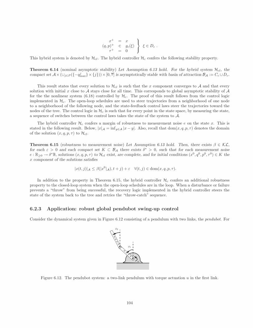
x+ = x(q, p)+ ∈ gc(ξ)

τ+ = 0

ξ ∈ Dc .

This hybrid system is denoted by Hcl. The hybrid controller Hc confers the following stability property.

Theorem 6.14 (nominal asymptotic stability) Let Assumption 6.13 hold. For the hybrid system Hcl, thecompact set A× (∪j∈P (−qj

max×j))× [0, τ] is asymptotically stable with basin of attraction BA := Cc ∪Dc.

This result states that every solution to Hcl is such that the x component converges to A and that everysolution with initial x close to A stays close for all time. This corresponds to global asymptotic stability of Afor the the nonlinear system (6.18) controlled by Hc. The proof of this result follows from the control logicimplemented in Hc. The open-loop schedules are used to steer trajectories from a neighborhood of one nodeto a neighborhood of the following node, and the state-feedback control laws steer the trajectories toward thenodes of the tree. The control logic in Hc is such that for every point in the state space, by measuring the state,a sequence of switches between the control laws takes the state of the system to A.

The hybrid controller Hc confers a margin of robustness to measurement noise e on the state x. This isstated in the following result. Below, |x|A = infy∈A |x− y|. Also, recall that dom(x, q, p, τ) denotes the domainof the solution (x, q, p, τ) to Hcl.

Theorem 6.15 (robustness to measurement noise) Let Assumption 6.13 hold. Then, there exists β ∈ KL,for each ε > 0 and each compact set K ⊂ BA there exists δ∗ > 0, such that for each measurement noisee : R≥0 → δ∗B, solutions (x, q, p, τ) to Hcl exist, are complete, and for initial conditions (x0, q0, p0, τ0) ∈ K thex component of the solutions satisfies

|x(t, j)|A ≤ β(|x0|A), t+ j) + ε ∀(t, j) ∈ dom(x, q, p, τ).

In addition to the property in Theorem 6.15, the hybrid controller Hc confers an additional robustnessproperty to the closed-loop system when the open-loop schedules are in the loop. When a disturbance or failureprevents a “throw” from being successful, the recovery logic implemented in the hybrid controller steers thestate of the system back to the tree and retries the “throw-catch” sequence.

6.2.3 Application: robust global pendubot swing-up control

Consider the dynamical system given in Figure 6.12 consisting of a pendulum with two links, the pendubot. For

u

φ1

φ2

Figure 6.12. The pendubot system: a two-link pendulum with torque actuation u in the first link.

104

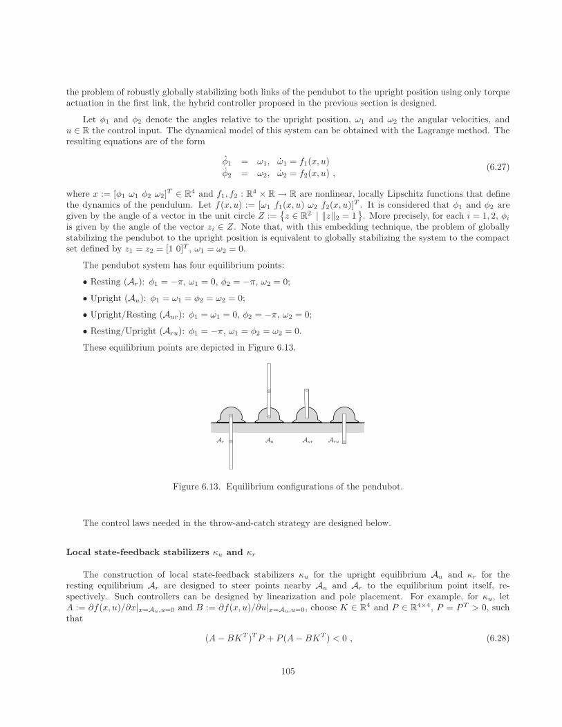
the problem of robustly globally stabilizing both links of the pendubot to the upright position using only torqueactuation in the first link, the hybrid controller proposed in the previous section is designed.

Let φ1 and φ2 denote the angles relative to the upright position, ω1 and ω2 the angular velocities, andu ∈ R the control input. The dynamical model of this system can be obtained with the Lagrange method. Theresulting equations are of the form

φ1 = ω1, ω1 = f1(x, u)

φ2 = ω2, ω2 = f2(x, u) ,(6.27)

where x := [φ1 ω1 φ2 ω2]T ∈ R

4 and f1, f2 : R4 × R → R are nonlinear, locally Lipschitz functions that define

the dynamics of the pendulum. Let f(x, u) := [ω1 f1(x, u) ω2 f2(x, u)]T . It is considered that φ1 and φ2 are

given by the angle of a vector in the unit circle Z :=z ∈ R

2 | ‖z‖2 = 1. More precisely, for each i = 1, 2, φi

is given by the angle of the vector zi ∈ Z. Note that, with this embedding technique, the problem of globallystabilizing the pendubot to the upright position is equivalent to globally stabilizing the system to the compactset defined by z1 = z2 = [1 0]T , ω1 = ω2 = 0.

The pendubot system has four equilibrium points:

• Resting (Ar): φ1 = −π, ω1 = 0, φ2 = −π, ω2 = 0;

• Upright (Au): φ1 = ω1 = φ2 = ω2 = 0;

• Upright/Resting (Aur): φ1 = ω1 = 0, φ2 = −π, ω2 = 0;

• Resting/Upright (Aru): φ1 = −π, ω1 = φ2 = ω2 = 0.

These equilibrium points are depicted in Figure 6.13.

Ar Au Aur Aru

Figure 6.13. Equilibrium configurations of the pendubot.

The control laws needed in the throw-and-catch strategy are designed below.

Local state-feedback stabilizers κu and κr

The construction of local state-feedback stabilizers κu for the upright equilibrium Au and κr for theresting equilibrium Ar are designed to steer points nearby Au and Ar to the equilibrium point itself, re-spectively. Such controllers can be designed by linearization and pole placement. For example, for κu, letA := ∂f(x, u)/∂x|x=Au,u=0 and B := ∂f(x, u)/∂u|x=Au,u=0, choose K ∈ R

4 and P ∈ R4×4, P = PT > 0, such

that

(A−BKT )TP + P (A−BKT ) < 0 , (6.28)

105

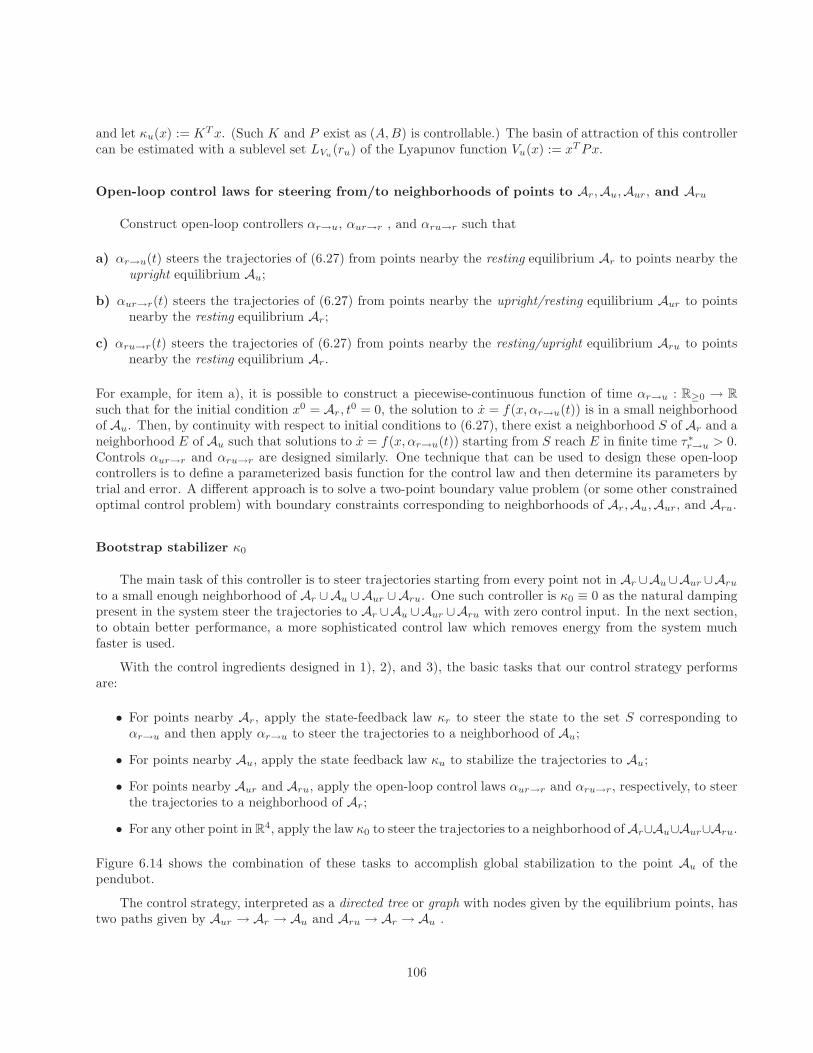
and let κu(x) := KTx. (Such K and P exist as (A,B) is controllable.) The basin of attraction of this controllercan be estimated with a sublevel set LVu

(ru) of the Lyapunov function Vu(x) := xTPx.

Open-loop control laws for steering from/to neighborhoods of points to Ar,Au,Aur, and Aru

Construct open-loop controllers αr→u, αur→r , and αru→r such that

a) αr→u(t) steers the trajectories of (6.27) from points nearby the resting equilibrium Ar to points nearby theupright equilibrium Au;

b) αur→r(t) steers the trajectories of (6.27) from points nearby the upright/resting equilibrium Aur to pointsnearby the resting equilibrium Ar;

c) αru→r(t) steers the trajectories of (6.27) from points nearby the resting/upright equilibrium Aru to pointsnearby the resting equilibrium Ar.

For example, for item a), it is possible to construct a piecewise-continuous function of time αr→u : R≥0 → R

such that for the initial condition x0 = Ar, t0 = 0, the solution to x = f(x, αr→u(t)) is in a small neighborhood

of Au. Then, by continuity with respect to initial conditions to (6.27), there exist a neighborhood S of Ar and aneighborhood E of Au such that solutions to x = f(x, αr→u(t)) starting from S reach E in finite time τ∗r→u > 0.Controls αur→r and αru→r are designed similarly. One technique that can be used to design these open-loopcontrollers is to define a parameterized basis function for the control law and then determine its parameters bytrial and error. A different approach is to solve a two-point boundary value problem (or some other constrainedoptimal control problem) with boundary constraints corresponding to neighborhoods of Ar,Au,Aur, and Aru.

Bootstrap stabilizer κ0

The main task of this controller is to steer trajectories starting from every point not in Ar ∪Au ∪Aur ∪Aru

to a small enough neighborhood of Ar ∪Au ∪Aur ∪Aru. One such controller is κ0 ≡ 0 as the natural dampingpresent in the system steer the trajectories to Ar ∪Au ∪Aur ∪Aru with zero control input. In the next section,to obtain better performance, a more sophisticated control law which removes energy from the system muchfaster is used.

With the control ingredients designed in 1), 2), and 3), the basic tasks that our control strategy performsare:

• For points nearby Ar, apply the state-feedback law κr to steer the state to the set S corresponding toαr→u and then apply αr→u to steer the trajectories to a neighborhood of Au;

• For points nearby Au, apply the state feedback law κu to stabilize the trajectories to Au;

• For points nearby Aur and Aru, apply the open-loop control laws αur→r and αru→r, respectively, to steerthe trajectories to a neighborhood of Ar;

• For any other point in R4, apply the law κ0 to steer the trajectories to a neighborhood of Ar∪Au∪Aur∪Aru.

Figure 6.14 shows the combination of these tasks to accomplish global stabilization to the point Au of thependubot.

The control strategy, interpreted as a directed tree or graph with nodes given by the equilibrium points, hastwo paths given by Aur → Ar → Au and Aru → Ar → Au .

106

αr→u

αru→u

κu

φ1

φ2

Ar

Au

Aur

Aru

LVu(ru)

LVr(rr)

κr(x)

κ0(x)

Sr→u

Er→u

Sru→r

Eru→u

Figure 6.14. Control strategy for robust global stabilization of the pendubot to the point Au. A sample trajectoryin the φ1, φ2 plane resulting from our control strategy is depicted. From the initial point ×, the trajectory issteered to the neighborhood Sru→r of Aru with κ0(x), from which it is “thrown” to the neighborhood Eru→r

of Ar with the control law αru→r. The local stabilizer κr “catches” the state to a point in Sr→u from wherethe open-loop law αr→u is applied. Finally, after the “throw”, the state reaches a point in Er→u and the last“catch” by the local stabilizer κu steers the trajectory to Au.

The nodes in each of the paths are numbered, starting from Aur and Aru and finishing at Au, by the pairs(i, j) ∈ 1, 2, 3 × 1, 2 where i indicates the node number and j the path number. Then, the two paths are

Path 1: (1, 1) → (2, 1) → (3, 1) (i.e. Aur → Ar → Au).

Path 2: (1, 2) → (2, 2) → (3, 2) (i.e. Aru → Ar → Au).

Then controller logic states, q and p, are such that (q, p) ∈ −3,−2, 0, 1, 2×1, 2. The timer state is τ ∈ R.Recall that the state q indicates the mode of the controller, p indicates the current path of the trajectories,and τ keeps track of the time that the system has been in open loop. Let τ∗1,1 = τ∗ur→r, τ

∗1,2 = τ∗ru→r, and

τ∗2,1 = τ∗2,2 = τ∗r→u. The control logic is summarized as follows:

• Catch mode when q < 0. This mode indicates that the state x is steered to the (|q|, p)-th node of thecurrent path p. If q = −2 then the control law applied is κr, while if q = −3 then the control law appliedis κu.

• Throw mode when q > 0. This mode indicates that the trajectories are being steered from a neighborhoodof the (q, p)-th node to a neighborhood of the (q+1, p)-th node of the current path p. If q = 1, p = 1, thenthe control law applied is αur→r; if q = 1, p = 2, then αru→r is applied; and if q = 2 then αr→u is applied.

• Recovery mode when q = p = 0. This mode indicates that the trajectories are being steered to the treewith the control law κ0.

The hybrid controller updates its state under the following events:

(C) “Throw-to-catch” transitions: when the state x is in some neighborhood E of an open-loop controllaw and in throw mode (q > 0), the controller jumps to catch mode (q updated to −(|q| + 1)). The timerstate τ is reset to zero.

107

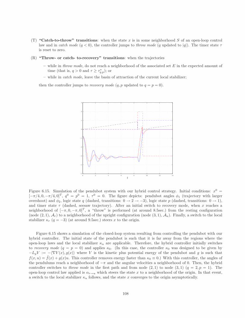
(T) “Catch-to-throw” transitions: when the state x is in some neighborhood S of an open-loop controllaw and in catch mode (q < 0), the controller jumps to throw mode (q updated to |q|). The timer state τis reset to zero.

(R) “Throw- or catch- to-recovery” transitions: when the trajectories

– while in throw mode, do not reach a neighborhood of the associated set E in the expected amount oftime (that is, q > 0 and τ ≥ τ∗q,p); or

– while in catch mode, leave the basin of attraction of the current local stabilizer;

then the controller jumps to recovery mode (q, p updated to q = p = 0).

t

0

0

2

2 4 6 8 10 12 14

1

3

−1

−2

−3

−4

−5

Figure 6.15. Simulation of the pendubot system with our hybrid control strategy. Initial conditions: x0 =[−π/4, 0,−π/4, 0]T , q0 = p0 = 1, τ0 = 0. The figure depicts: pendubot angles φ1 (trajectory with largerovershoot) and φ2, logic state q (dashed, transitions: 0 → 2 → −3), logic state p (dashed, transitions: 0 → 1),and timer state τ (dashed, seesaw trajectory). After an initial switch to recovery mode, when x reaches aneighborhood of [−π, 0,−π, 0]T , a “throw” is performed (at around 8.5sec.) from the resting configuration(node (2, 1), Ar) to a neighborhood of the upright configuration (node (3, 1), Au). Finally, a switch to the localstabilizer κr (q = −3) (at around 9.5sec.) steers x to the origin.

Figure 6.15 shows a simulation of the closed-loop system resulting from controlling the pendubot with ourhybrid controller. The initial state of the pendubot is such that it is far away from the regions where theopen-loop laws and the local stabilizer κu are applicable. Therefore, the hybrid controller initially switchesto recovery mode (q = p = 0) and applies κ0. (In this case, the controller κ0 was designed to be given by−LgV := −〈∇V (x), g(x)〉 where V is the kinetic plus potential energy of the pendubot and g is such that

f(x, u) = f(x) + g(x)u. This controller removes energy faster than κ0 ≡ 0.) With this controller, the angles ofthe pendulums reach a neighborhood of −π and the angular velocities a neighborhood of 0. Then, the hybridcontroller switches to throw mode in the first path and from node (2, 1) to node (3, 1) (q = 2, p = 1). Theopen-loop control law applied is αr→u which steers the state x to a neighborhood of the origin. In that event,a switch to the local stabilizer κu follows, and the state x converges to the origin asymptotically.

108

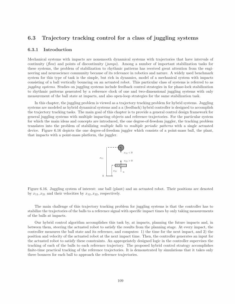
6.3 Trajectory tracking control for a class of juggling systems

6.3.1 Introduction

Mechanical systems with impacts are nonsmooth dynamical systems with trajectories that have intervals ofcontinuity (flow) and points of discontinuity (jumps). Among a number of important stabilization tasks forthese systems, the problem of stabilization to rhythmic patterns has received great attention from the engi-neering and neuroscience community because of its relevance in robotics and nature. A widely used benchmarksystem for this type of task is the simple, but rich in dynamics, model of a mechanical system with impactsconsisting of a ball vertically bouncing on an actuated robot. This particular class of systems is referred to asjuggling systems. Studies on juggling systems include feedback control strategies in for phase-lock stabilizationto rhythmic patterns generated by a reference clock of one and two-dimensional juggling systems with onlymeasurement of the ball state at impacts, and also open-loop strategies for the same stabilization task.

In this chapter, the juggling problem is viewed as a trajectory tracking problem for hybrid systems. Jugglingsystems are modeled as hybrid dynamical systems and a a (feedback) hybrid controller is designed to accomplishthe trajectory tracking tasks. The main goal of this chapter is to provide a general control design framework forgeneral juggling systems with multiple impacting objects and reference trajectories. For the particular systemfor which the main ideas and concepts are introduced, the one degree-of-freedom juggler, the tracking problemtranslates into the problem of stabilizing multiple balls to multiple periodic patterns with a single actuateddevice. Figure 6.16 depicts the one degree-of-freedom juggler which consists of a point-mass ball, the plant,that impacts with a point-mass platform, the juggler.

x11

x12 < 0

x21

x22 > 0

u

0

Figure 6.16. Juggling system of interest: one ball (plant) and an actuated robot. Their positions are denotedby x11, x21 and their velocities by x12, x22, respectively.

The main challenge of this trajectory tracking problem for juggling systems is that the controller has tostabilize the trajectories of the balls to a reference signal with specific impact times by only taking measurementsof the balls at impacts.

Our hybrid control algorithm accomplishes this task by, at impacts, planning the future impacts and, inbetween them, steering the actuated robot to satisfy the results from the planning stage. At every impact, thecontroller measures the ball state and its reference, and computes: 1) the time for the next impact, and 2) theposition and velocity of the actuated robot at the next impact time. Then, the controller generates an input forthe actuated robot to satisfy these constraints. An appropriately designed logic in the controller supervises thetracking of each of the balls to each reference trajectory. The proposed hybrid control strategy accomplishesfinite-time practical tracking of the reference trajectories. It is demonstrated by simulations that it takes onlythree bounces for each ball to approach the reference trajectories.

109

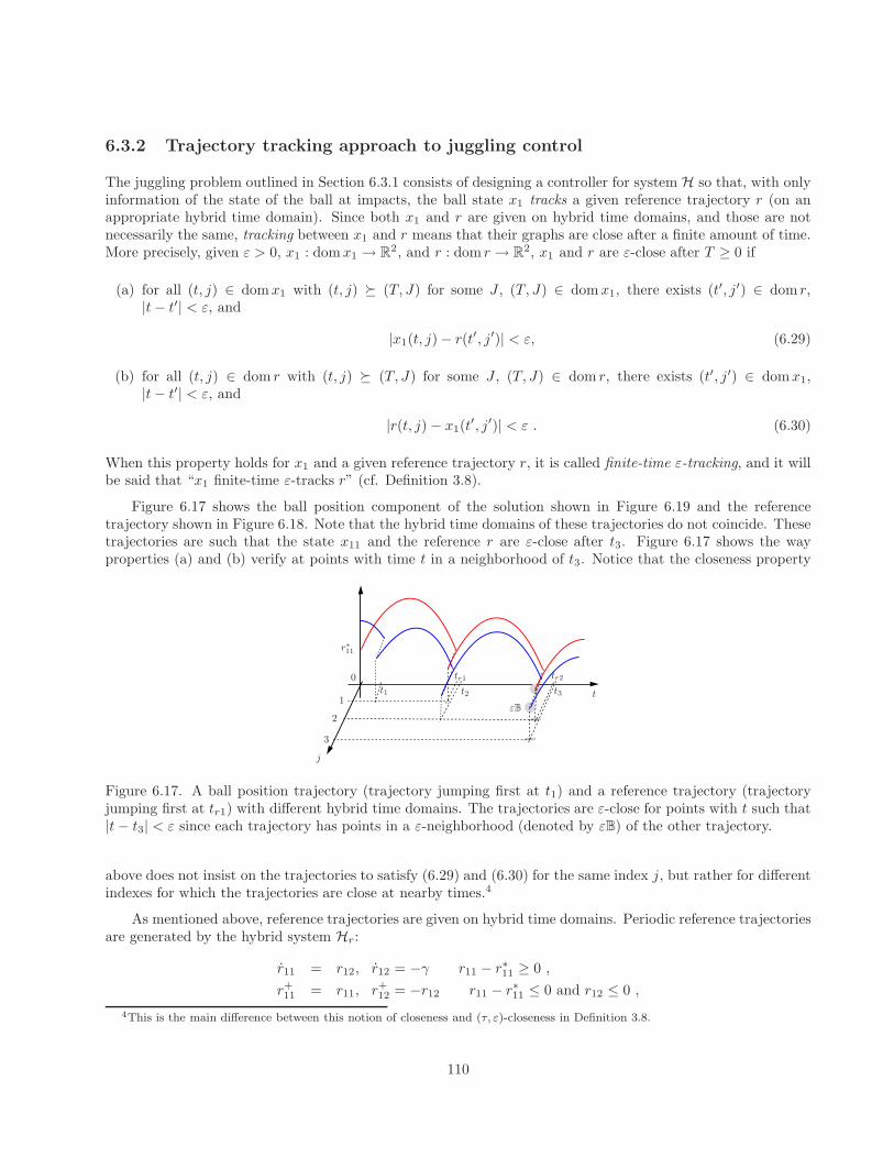
6.3.2 Trajectory tracking approach to juggling control

The juggling problem outlined in Section 6.3.1 consists of designing a controller for system H so that, with onlyinformation of the state of the ball at impacts, the ball state x1 tracks a given reference trajectory r (on anappropriate hybrid time domain). Since both x1 and r are given on hybrid time domains, and those are notnecessarily the same, tracking between x1 and r means that their graphs are close after a finite amount of time.More precisely, given ε > 0, x1 : domx1 → R

2, and r : dom r → R2, x1 and r are ε-close after T ≥ 0 if

(a) for all (t, j) ∈ domx1 with (t, j) (T, J) for some J , (T, J) ∈ domx1, there exists (t′, j′) ∈ dom r,|t− t′| < ε, and

|x1(t, j) − r(t′, j′)| < ε, (6.29)

(b) for all (t, j) ∈ dom r with (t, j) (T, J) for some J , (T, J) ∈ dom r, there exists (t′, j′) ∈ domx1,|t− t′| < ε, and

|r(t, j) − x1(t′, j′)| < ε . (6.30)

When this property holds for x1 and a given reference trajectory r, it is called finite-time ε-tracking, and it willbe said that “x1 finite-time ε-tracks r” (cf. Definition 3.8).

Figure 6.17 shows the ball position component of the solution shown in Figure 6.19 and the referencetrajectory shown in Figure 6.18. Note that the hybrid time domains of these trajectories do not coincide. Thesetrajectories are such that the state x11 and the reference r are ε-close after t3. Figure 6.17 shows the wayproperties (a) and (b) verify at points with time t in a neighborhood of t3. Notice that the closeness property

1

2

3

t

tr1 tr2

t1 t2 t3

j

0

r∗11

εB

Figure 6.17. A ball position trajectory (trajectory jumping first at t1) and a reference trajectory (trajectoryjumping first at tr1) with different hybrid time domains. The trajectories are ε-close for points with t such that|t− t3| < ε since each trajectory has points in a ε-neighborhood (denoted by εB) of the other trajectory.

above does not insist on the trajectories to satisfy (6.29) and (6.30) for the same index j, but rather for differentindexes for which the trajectories are close at nearby times.4

As mentioned above, reference trajectories are given on hybrid time domains. Periodic reference trajectoriesare generated by the hybrid system Hr:

r11 = r12, r12 = −γ r11 − r∗11 ≥ 0 ,

r+11 = r11, r+12 = −r12 r11 − r∗11 ≤ 0 and r12 ≤ 0 ,

4This is the main difference between this notion of closeness and (τ, ε)-closeness in Definition 3.8.

110

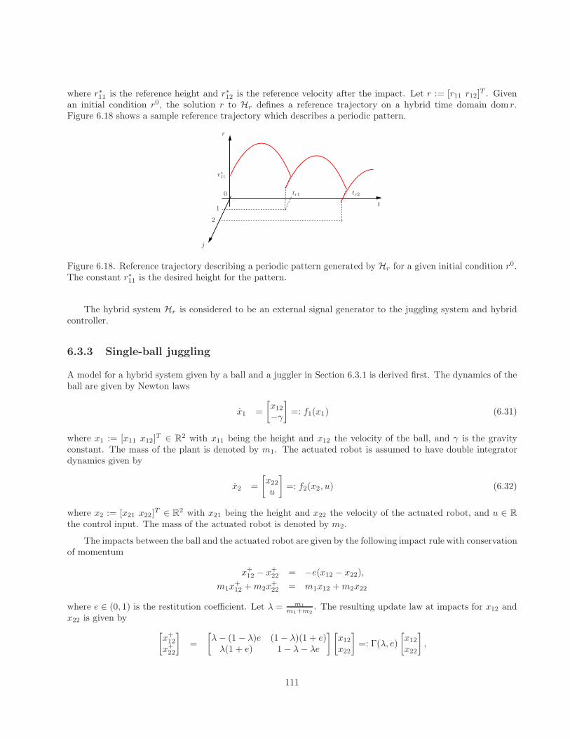
where r∗11 is the reference height and r∗12 is the reference velocity after the impact. Let r := [r11 r12]T . Given

an initial condition r0, the solution r to Hr defines a reference trajectory on a hybrid time domain dom r.Figure 6.18 shows a sample reference trajectory which describes a periodic pattern.

1

2

t

tr1 tr2

j

0

r

r∗11

Figure 6.18. Reference trajectory describing a periodic pattern generated by Hr for a given initial condition r0.The constant r∗11 is the desired height for the pattern.

The hybrid system Hr is considered to be an external signal generator to the juggling system and hybridcontroller.

6.3.3 Single-ball juggling

A model for a hybrid system given by a ball and a juggler in Section 6.3.1 is derived first. The dynamics of theball are given by Newton laws

x1 =

[x12

−γ

]=: f1(x1) (6.31)

where x1 := [x11 x12]T ∈ R

2 with x11 being the height and x12 the velocity of the ball, and γ is the gravityconstant. The mass of the plant is denoted by m1. The actuated robot is assumed to have double integratordynamics given by

x2 =

[x22

u

]=: f2(x2, u) (6.32)

where x2 := [x21 x22]T ∈ R

2 with x21 being the height and x22 the velocity of the actuated robot, and u ∈ R

the control input. The mass of the actuated robot is denoted by m2.

The impacts between the ball and the actuated robot are given by the following impact rule with conservationof momentum

x+12 − x+

22 = −e(x12 − x22),

m1x+12 +m2x

+22 = m1x12 +m2x22

where e ∈ (0, 1) is the restitution coefficient. Let λ = m1

m1+m2. The resulting update law at impacts for x12 and

x22 is given by

[x+

12

x+22

]=

[λ− (1 − λ)e (1 − λ)(1 + e)λ(1 + e) 1 − λ− λe

] [x12

x22

]=: Γ(λ, e)

[x12

x22

],

111

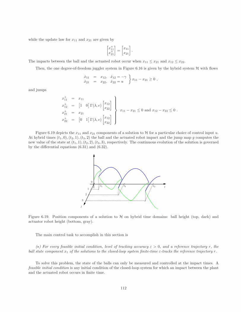
while the update law for x11 and x21 are given by

[x+

11

x+21

]=

[x11

x21

].

The impacts between the ball and the actuated robot occur when x11 ≤ x21 and x12 ≤ x22.

Then, the one degree-of-freedom juggler system in Figure 6.16 is given by the hybrid system H with flows

x11 = x12, x12 = −γx21 = x22, x22 = u

x11 − x21 ≥ 0 ,

and jumps

x+11 = x11

x+12 =

[1 0

]Γ(λ, e)

[x12

x22

]

x+21 = x21

x+22 =

[0 1

]Γ(λ, e)

[x12

x22

]

x11 − x21 ≤ 0 and x12 − x22 ≤ 0 .

Figure 6.19 depicts the x11 and x21 components of a solution to H for a particular choice of control input u.At hybrid times (t1, 0), (t2, 1), (t3, 2) the ball and the actuated robot impact and the jump map g computes thenew value of the state at (t1, 1), (t2, 2), (t3, 3), respectively. The continuous evolution of the solution is governedby the differential equations (6.31) and (6.32).

1

2

3

tt1 t2 t3

j

0

Figure 6.19. Position components of a solution to H on hybrid time domains: ball height (top, dark) andactuator robot height (bottom, gray).

The main control task to accomplish in this section is

(⋆) For every feasible initial condition, level of tracking accuracy ε > 0, and a reference trajectory r, theball state component x1 of the solutions to the closed-loop system finite-time ε-tracks the reference trajectory r.

To solve this problem, the state of the balls can only be measured and controlled at the impact times. Afeasible initial condition is any initial condition of the closed-loop system for which an impact between the plantand the actuated robot occurs in finite time.

112

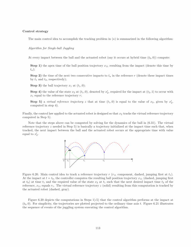
Control strategy

The main control idea to accomplish the tracking problem in (⋆) is summarized in the following algorithm:

Algorithm for Single-ball Juggling

At every impact between the ball and the actuated robot (say it occurs at hybrid time (t0, 0)) compute:

Step 1) the apex time of the ball position trajectory x11 resulting from the impact (denote this time byta);

Step 2) the time of the next two consecutive impacts to ta in the reference r (denote these impact timesby t1 and t2, respectively);

Step 3) the ball trajectory x1 at (t1, 0);

Step 4) the value of the state x2 at (t1, 0), denoted by x′2, required for the impact at (t2, 1) to occur withx1 equal to the reference trajectory r;

Step 5) a virtual reference trajectory z that at time (t1, 0) is equal to the value of x2, given by x′2,computed in step 4).

Finally, the control law applied to the actuated robot is designed so that x2 tracks the virtual reference trajectorycomputed in Step 5).

Note that the steps above can be computed by solving for the dynamics of the ball in (6.31). The virtualreference trajectory z needed in Step 5) is basically a trajectory initialized at the impact time such that, whentracked, the next impact between the ball and the actuated robot occurs at the appropriate time with valueequal to x′2.

0 t0 t1 t2 t

Figure 6.20. Main control idea to track a reference trajectory r (r11 component, dashed, jumping first at t1).At the impact at t = t0, the controller computes the resulting ball position trajectory x11 (dashed, jumping firstat t0) at time t1 and the required value of the state x2 at t1 such that the next desired impact time t2 of thereference, x11 equals r1. The virtual reference trajectory z (solid) resulting from this computation is tracked bythe actuated robot (dashed, gray).

Figure 6.20 depicts the computations in Steps 1)-5) that the control algorithm performs at the impact at(t0, 0). For simplicity, the trajectories are plotted projected to the ordinary time axis t. Figure 6.21 illustratesthe sequence of events of the juggling system executing the control algorithm.

113

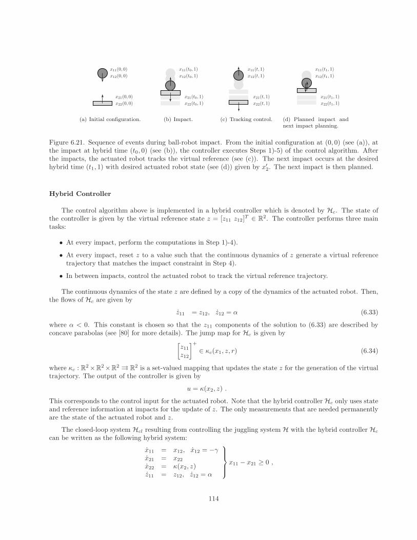
x11(0, 0)

x12(0, 0)

x21(0, 0)

x22(0, 0)

(a) Initial configuration.

x11(t0, 1)

x12(t0, 1)

x21(t0, 1)

x22(t0, 1)

(b) Impact.

x11(t, 1)

x12(t, 1)

x21(t, 1)

x22(t, 1)

(c) Tracking control.

x11(t1, 1)

x12(t1, 1)

x21(t1, 1)

x22(t1, 1)

(d) Planned impact andnext impact planning.

Figure 6.21. Sequence of events during ball-robot impact. From the initial configuration at (0, 0) (see (a)), atthe impact at hybrid time (t0, 0) (see (b)), the controller executes Steps 1)-5) of the control algorithm. Afterthe impacts, the actuated robot tracks the virtual reference (see (c)). The next impact occurs at the desiredhybrid time (t1, 1) with desired actuated robot state (see (d)) given by x′2. The next impact is then planned.

Hybrid Controller

The control algorithm above is implemented in a hybrid controller which is denoted by Hc. The state ofthe controller is given by the virtual reference state z = [z11 z12]

T ∈ R2. The controller performs three main

tasks:

• At every impact, perform the computations in Step 1)-4).

• At every impact, reset z to a value such that the continuous dynamics of z generate a virtual referencetrajectory that matches the impact constraint in Step 4).

• In between impacts, control the actuated robot to track the virtual reference trajectory.

The continuous dynamics of the state z are defined by a copy of the dynamics of the actuated robot. Then,the flows of Hc are given by

z11 = z12, z12 = α (6.33)

where α < 0. This constant is chosen so that the z11 components of the solution to (6.33) are described byconcave parabolas (see [80] for more details). The jump map for Hc is given by

[z11z12

]+

∈ κc(x1, z, r) (6.34)

where κc : R2 ×R

2×R2 →→ R

2 is a set-valued mapping that updates the state z for the generation of the virtualtrajectory. The output of the controller is given by

u = κ(x2, z) .

This corresponds to the control input for the actuated robot. Note that the hybrid controller Hc only uses stateand reference information at impacts for the update of z. The only measurements that are needed permanentlyare the state of the actuated robot and z.

The closed-loop system Hcl resulting from controlling the juggling system H with the hybrid controller Hc

can be written as the following hybrid system:

x11 = x12, x12 = −γx21 = x22

x22 = κ(x2, z)z11 = z12, z12 = α

x11 − x21 ≥ 0 ,

114

x+11 = x11

x+12 =

[1 0

]Γ(λ, e)

[x12

x22

]

x+21 = x21

x+22 =

[0 1

]Γ(λ, e)

[x12

x22

]

[z11z12

]+

∈ κc(x1, z, r)

x11 − x21 ≤ 0 and x12 − x22 ≤ 0 .

This construction is such that Hcl satisfies the hybrid basic conditions.

Control Design

To design the update law κc of the hybrid controller Hc, the dynamics of the actuated robot in H areinitially replaced by the dynamics of the state z in Hc, i.e.,

x11 = x12, x12 = −γz11 = z12, z12 = α

x11 − z11 ≥ 0 ,

x+11 = x11

x+12 =

[1 0

]Γ(λ, e)

[x12

z12

]

[z11z12

]+

∈ κc(x1, z, r)

x11 − z11 ≤ 0 and x12 − z12 ≤ 0 .

This system is denoted by Hv, meaning virtual juggling system. The main idea for control design is to definethe set-valued map κc such that the control task (⋆) is accomplished for Hv and then design a control law κthat acts on the actuated robot and accomplishes (standard) tracking between x2 and r. To that end, a resultfor the solutions to Hv is first stated.

Lemma 6.16 (property of solutions to Hv) For every feasible initial condition

[x11(0, 0) x12(0, 0) z11(0, 0) z12(0, 0)]T

for Hv, the next impact occurs at time (t1, 0) provided that

z11(0, 0) = −γ + α

2t21 + (x12(0, 0) − z12(0, 0))t1 + x11(0, 0) . (6.35)

Moreover, the position and velocity of the ball after the impact at (t1, 0), denoted by x11(t1, 1) and x12(t1, 1),respectively, are given by

x11(t1, 1) = −γ2t21 + x12(0, 0)t1 + x11(0, 0), (6.36)

x12(t1, 1) =[1 0

]Γ(λ, e)

[x12(0, 0) − γt1αt1 + z12(0, 0)

]. (6.37)

Proof. Given a feasible initial condition [x11(0, 0) x12(0, 0) z11(0, 0) z12(0, 0)]T , that is, an initial condition forwhich there exists t1 > 0 such that an impact between the ball and the virtual reference occurs at (t1, 0), then,up to (t1, 0), the ball trajectory is given by

x11(t, 0) = −γ2t2 + x12(0, 0)t+ x11 (6.38)

x12(t, 0) = −γt+ x12(0, 0) (6.39)

115

and for the virtual reference

z11(t, 0) =α

2t2 + z12(0, 0)t+ z11 (6.40)

z12(t, 0) = αt+ z12(0, 0) . (6.41)

For the impact to occur at (t1, 0), x11(t1, 0) = z11(t1, 0) and x12(t1, 0) ≤ z12(t1, 0). The first conditionimplies (6.35). The second condition is satisfied by the initial condition being feasible.

Finally, (6.36) and (6.37) are given by applying the jump map of Hv to x and z at (t1, 0).

Lemma 6.16 can be shown by solving the continuous dynamics of the ball and state z. In fact, equation(6.35) follows from solving the system backward in time from the jump condition of Hv, equation (6.36) followsfrom the fact that the x11 component of the solution is mapped to itself at jumps, and equation (6.37) is derivedfrom the impact rule used for the impacts of Hv.

Let J : R2 × R

2 × R2 →→ R

2 be the set-valued mapping

J(x1, z, r) =

r12+r∗12

γ if ax12+bz12

γ <r12+r∗

12

γr12+r∗

12

γ ,r12+r∗

12

γ + Tr

if ax12+bz12

γ =r12+r∗

12

γr12+r∗

12

γ + Tr if ax12+bz12

γ >r12+r∗

12

γ

(6.42)

where Tr = 2r∗12/γ and

a =[1 0

]Γ(λ, e)

[10

], b =

[1 0

]Γ(λ, e)

[01

].

The proposed control algorithm first computes the time for the next impact t1 in Step 1) and then computesStep 2)-5) to generate a virtual trajectory. Regarding Step 1), the set-valued mapping J contains the time(s)to the next impact t1 from the current state. The value of t1 is chosen so that if the apex time of the trajectoryx11 is smaller than the time for the next impact of the reference, then t1 is given by the next impact time ofthe reference. If it is larger, then the impact is postponed for one period Tr. When t1 is equal to the apex timeboth times are possible, and therefore, J is set-valued. Regarding Step 2)-5), for each t1 ∈ J(x1, z, r), the resetvalue z∗ for z is computed by two applications of Lemma 6.16. This is done by setting x11(t1 + Tr, 3) = r∗11and x12(t1 + Tr, 3) = r∗12 (see Figure 6.20). Then, the set-valued mapping κc(x1, z, r) is given by all pointsz∗ = [z∗11 z

∗12]

T such that

z∗11 = −γ + α

2t21 + (ax12 + bz12 − z∗12)t1 + x11

(6.43)

z∗12 =r∗11 + γ

2T2r + γ

2 t21 − (ax12 + bz12)t1 − x11

bTr+

(aγ − bα)t1 − a(ax12 + bz12)

b.

(6.44)

The control law κ is designed so that the trajectories of the platform system track the trajectories of thevirtual platform system. Let e1 := x21 − z11, e2 := x22 − z12. Then, the error system is

e1 = e2, e2 = u− α .

Given k1, k2 > 0, a particular choice of the control law κ to accomplish the tracking between x2 and r is givenby

κ(x2, z) = α− k1(x21 − z11) − k2(x22 − z12) .

116

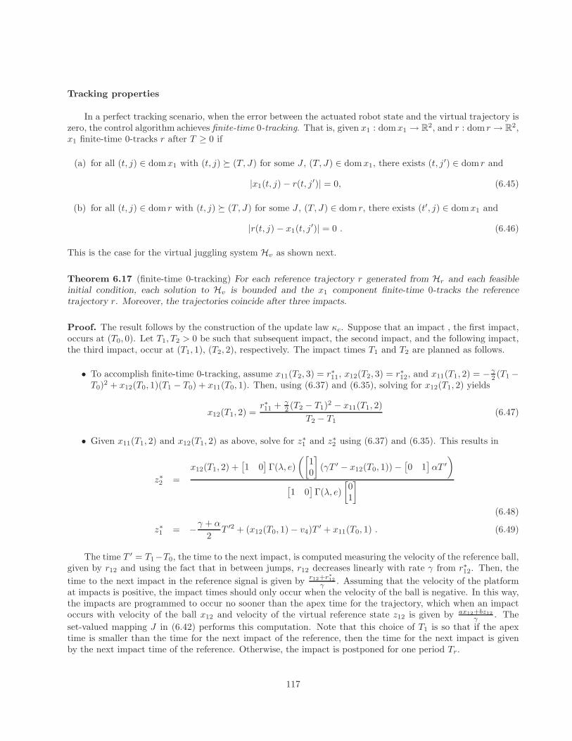
Tracking properties

In a perfect tracking scenario, when the error between the actuated robot state and the virtual trajectory iszero, the control algorithm achieves finite-time 0-tracking. That is, given x1 : domx1 → R

2, and r : dom r → R2,

x1 finite-time 0-tracks r after T ≥ 0 if

(a) for all (t, j) ∈ domx1 with (t, j) (T, J) for some J , (T, J) ∈ domx1, there exists (t, j′) ∈ dom r and

|x1(t, j) − r(t, j′)| = 0, (6.45)

(b) for all (t, j) ∈ dom r with (t, j) (T, J) for some J , (T, J) ∈ dom r, there exists (t′, j) ∈ domx1 and

|r(t, j) − x1(t, j′)| = 0 . (6.46)

This is the case for the virtual juggling system Hv as shown next.

Theorem 6.17 (finite-time 0-tracking) For each reference trajectory r generated from Hr and each feasibleinitial condition, each solution to Hv is bounded and the x1 component finite-time 0-tracks the referencetrajectory r. Moreover, the trajectories coincide after three impacts.

Proof. The result follows by the construction of the update law κc. Suppose that an impact , the first impact,occurs at (T0, 0). Let T1, T2 > 0 be such that subsequent impact, the second impact, and the following impact,the third impact, occur at (T1, 1), (T2, 2), respectively. The impact times T1 and T2 are planned as follows.

• To accomplish finite-time 0-tracking, assume x11(T2, 3) = r∗11, x12(T2, 3) = r∗12, and x11(T1, 2) = −γ2 (T1 −

T0)2 + x12(T0, 1)(T1 − T0) + x11(T0, 1). Then, using (6.37) and (6.35), solving for x12(T1, 2) yields

x12(T1, 2) =r∗11 + γ

2 (T2 − T1)2 − x11(T1, 2)

T2 − T1(6.47)

• Given x11(T1, 2) and x12(T1, 2) as above, solve for z∗1 and z∗2 using (6.37) and (6.35). This results in

z∗2 =

x12(T1, 2) +[1 0

]Γ(λ, e)

([10

](γT ′ − x12(T0, 1)) −

[0 1

]αT ′

)

[1 0

]Γ(λ, e)

[01

]

(6.48)

z∗1 = −γ + α

2T ′2 + (x12(T0, 1) − v4)T

′ + x11(T0, 1) . (6.49)

The time T ′ = T1−T0, the time to the next impact, is computed measuring the velocity of the reference ball,given by r12 and using the fact that in between jumps, r12 decreases linearly with rate γ from r∗12. Then, the

time to the next impact in the reference signal is given byr12+r∗

12

γ . Assuming that the velocity of the platformat impacts is positive, the impact times should only occur when the velocity of the ball is negative. In this way,the impacts are programmed to occur no sooner than the apex time for the trajectory, which when an impactoccurs with velocity of the ball x12 and velocity of the virtual reference state z12 is given by ax12+bz12

γ . The

set-valued mapping J in (6.42) performs this computation. Note that this choice of T1 is so that if the apextime is smaller than the time for the next impact of the reference, then the time for the next impact is givenby the next impact time of the reference. Otherwise, the impact is postponed for one period Tr.

117

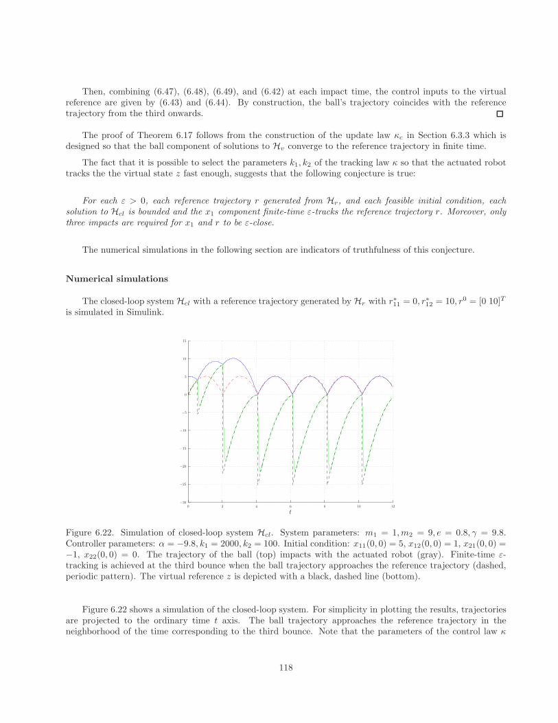
Then, combining (6.47), (6.48), (6.49), and (6.42) at each impact time, the control inputs to the virtualreference are given by (6.43) and (6.44). By construction, the ball’s trajectory coincides with the referencetrajectory from the third onwards.

The proof of Theorem 6.17 follows from the construction of the update law κc in Section 6.3.3 which isdesigned so that the ball component of solutions to Hv converge to the reference trajectory in finite time.

The fact that it is possible to select the parameters k1, k2 of the tracking law κ so that the actuated robottracks the the virtual state z fast enough, suggests that the following conjecture is true:

For each ε > 0, each reference trajectory r generated from Hr, and each feasible initial condition, eachsolution to Hcl is bounded and the x1 component finite-time ε-tracks the reference trajectory r. Moreover, onlythree impacts are required for x1 and r to be ε-close.

The numerical simulations in the following section are indicators of truthfulness of this conjecture.

Numerical simulations

The closed-loop system Hcl with a reference trajectory generated by Hr with r∗11 = 0, r∗12 = 10, r0 = [0 10]T

is simulated in Simulink.

0

0 2 4

5

6 8

10

10 12

15

−5

−10

−15

−20

−25

−30

t

Figure 6.22. Simulation of closed-loop system Hcl. System parameters: m1 = 1,m2 = 9, e = 0.8, γ = 9.8.Controller parameters: α = −9.8, k1 = 2000, k2 = 100. Initial condition: x11(0, 0) = 5, x12(0, 0) = 1, x21(0, 0) =−1, x22(0, 0) = 0. The trajectory of the ball (top) impacts with the actuated robot (gray). Finite-time ε-tracking is achieved at the third bounce when the ball trajectory approaches the reference trajectory (dashed,periodic pattern). The virtual reference z is depicted with a black, dashed line (bottom).

Figure 6.22 shows a simulation of the closed-loop system. For simplicity in plotting the results, trajectoriesare projected to the ordinary time t axis. The ball trajectory approaches the reference trajectory in theneighborhood of the time corresponding to the third bounce. Note that the parameters of the control law κ

118

0

0 2 4 6 8

10

10 12

−10

−20

20

30

−30

−40

−50

−60

−70

t

Figure 6.23. Simulation of closed-loop system Hcl. System parameters: m1 = 1,m2 = 9, e = 0.8, γ = 9.8.Controller parameters: α = −9.8, k1 = 2000, k2 = 100. Initial condition: x11(0, 0) = 5, x12(0, 0) = 1, x21(0, 0) =−1, x22(0, 0) = 0. The trajectory of the ball (top) impacts with the actuated robot (gray). Finite-time ε-tracking is achieved at the third bounce when the ball trajectory approaches the reference trajectory (dashed,periodic pattern). The virtual reference z is depicted with a black, dashed line (bottom).

steer the actuated robot to a very small neighborhood of the virtual reference as the figure indicates. This canbe adjusted appropriately with the parameters k1 and k2.

The simulation in Figure 6.23 is for the same reference trajectory but for different initial conditions of theball. It illustrates the decision that the controller makes when the apex time of the trajectory after the firstbounce is larger than the next impact of the reference trajectory. As a difference to the simulation in Figure 6.22,the second impact is planned for t1 = 4r∗12/γ rather than for t1 = 2r∗12/γ. Recall that the control algorithm isso that, if the apex time coincides with the impact time of the reference trajectory, both choices are possible.

6.3.4 Multiple-balls juggling control

In this section, the multiple balls juggling problem is considered. Suppose that n reference trajectories, n balls,and one actuated robot are given as in Figure 6.24. The goal is the following:

(⋆⋆) For every feasible initial condition and n reference trajectories with distinct impact times, the i-th ballstate component xi

1 of the solutions to the closed-loop system finite-time ε-tracks the i-th reference trajectory ri.

Recall that the state of the balls can only be measured and controlled at the impact times.

A feasible initial condition in this multiple trajectory tracking problem means any initial condition for whicheach ball impacts with the actuated robot in finite time and in an ordered manner: every n impacts, each ballhas impacted only once, and the order is preserved for all time.

119

x111

x112 < 0

x211

x212 < 0

xn11

xn12 < 0

x21

x22 > 0

u

0

Figure 6.24. Juggling system of interest: n balls (plant) and one actuated robot. The ball positions and velocitiesare denoted by xi

11, xi12, respectively, and the actuated robot position and velocity by x12, x22, respectively.

Control Strategy and Hybrid Controller

The control strategy proposed here combines the control algorithm introduced in Section 6.3.3 to plan theimpacts for each ball individually and uses additional logic to select the ball to control. Let Q := 1, 2, . . . , nand q be a logic state, q ∈ Q. Let zq ∈ R

2 be the virtual reference state of the q-th ball. The reference trajectoryfor q-th ball is generated by the hybrid system Hq

r . It is assumed that for each q, Hqr is defined as Hr. Moreover,

it is assumed that the reference trajectories are such that the impact times do not occur at the same time andthat they have the above ordering property: every n impacts, each reference trajectory has only one impact,and the order is preserved for all time.

The control logic for multi-ball juggling is as follows.

Algorithm for Multiple-balls Juggling

At an impact between the q-th ball and the actuated robot:

Step 1) With reference trajectory rq, compute Step 1)-5) of the Algorithm for Single-ball Juggling toobtain zq∗. Update the state zq with this value.

Step 2) Update the logic state q by q+= mod (q, n) + 1.

Step 3) Apply to the actuated robot a control law that tracks the virtual reference zq.

This logic is implemented in a hybrid controller resulting in the closed-loop system HMcl given by

120

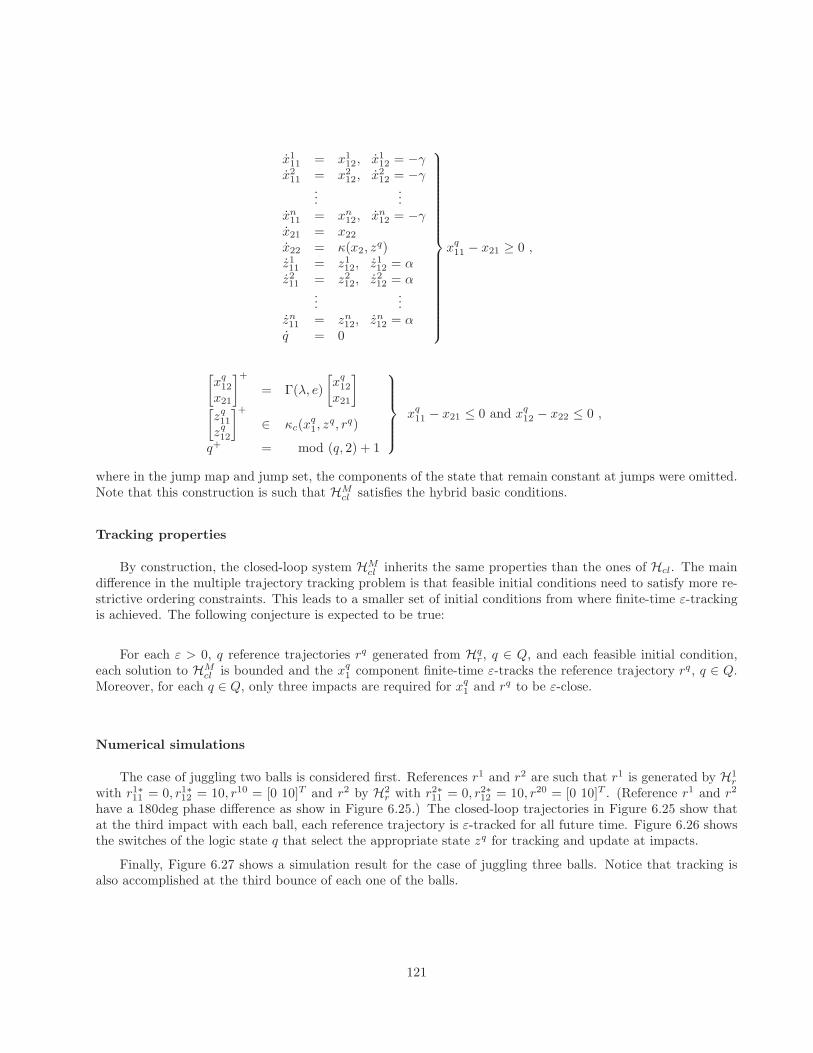
x111 = x1

12, x112 = −γ

x211 = x2

12, x212 = −γ

......

xn11 = xn

12, xn12 = −γ

x21 = x22

x22 = κ(x2, zq)

z111 = z1

12, z112 = α

z211 = z2

12, z212 = α

......

zn11 = zn

12, zn12 = α

q = 0

xq11 − x21 ≥ 0 ,

[xq

12

x21

]+

= Γ(λ, e)

[xq

12

x21

]

[zq11

zq12

]+

∈ κc(xq1, z

q, rq)

q+ = mod (q, 2) + 1

xq11 − x21 ≤ 0 and xq

12 − x22 ≤ 0 ,

where in the jump map and jump set, the components of the state that remain constant at jumps were omitted.Note that this construction is such that HM

cl satisfies the hybrid basic conditions.

Tracking properties

By construction, the closed-loop system HMcl inherits the same properties than the ones of Hcl. The main

difference in the multiple trajectory tracking problem is that feasible initial conditions need to satisfy more re-strictive ordering constraints. This leads to a smaller set of initial conditions from where finite-time ε-trackingis achieved. The following conjecture is expected to be true:

For each ε > 0, q reference trajectories rq generated from Hqr , q ∈ Q, and each feasible initial condition,

each solution to HMcl is bounded and the xq

1 component finite-time ε-tracks the reference trajectory rq , q ∈ Q.Moreover, for each q ∈ Q, only three impacts are required for xq

1 and rq to be ε-close.

Numerical simulations

The case of juggling two balls is considered first. References r1 and r2 are such that r1 is generated by H1r

with r1∗11 = 0, r1∗12 = 10, r10 = [0 10]T and r2 by H2r with r2∗11 = 0, r2∗12 = 10, r20 = [0 10]T . (Reference r1 and r2

have a 180deg phase difference as show in Figure 6.25.) The closed-loop trajectories in Figure 6.25 show thatat the third impact with each ball, each reference trajectory is ε-tracked for all future time. Figure 6.26 showsthe switches of the logic state q that select the appropriate state zq for tracking and update at impacts.

Finally, Figure 6.27 shows a simulation result for the case of juggling three balls. Notice that tracking isalso accomplished at the third bounce of each one of the balls.

121

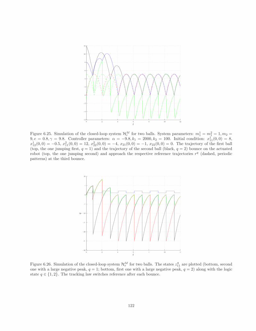
0

0

2

2

−2

4

4

−4

6

6−6

8

8

10

10

12

12

t

Figure 6.25. Simulation of the closed-loop system HMr for two balls. System parameters: m1

1 = m21 = 1,m2 =

9, e = 0.8, γ = 9.8. Controller parameters: α = −9.8, k1 = 2000, k2 = 100. Initial condition: x111(0, 0) = 8,

x112(0, 0) = −0.5, x2

11(0, 0) = 12, x222(0, 0) = −4, x21(0, 0) = −1, x22(0, 0) = 0. The trajectory of the first ball

(top, the one jumping first, q = 1) and the trajectory of the second ball (black, q = 2) bounce on the actuatedrobot (top, the one jumping second) and approach the respective reference trajectories rq (dashed, periodicpatterns) at the third bounce.

0

0 2 4

5

6 8

10

10 12

−5

−10

−15

−20

−25

−30

t

q

Figure 6.26. Simulation of the closed-loop system HMr for two balls. The states zq

11 are plotted (bottom, secondone with a large negative peak, q = 1; bottom, first one with a large negative peak, q = 2) along with the logicstate q ∈ 1, 2. The tracking law switches reference after each bounce.

122

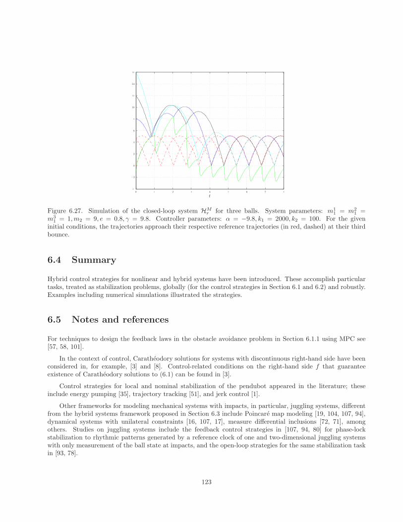
0

0 1

2

2 3

4

4 5

6

6

8

8

10

12

14

16

−2

4

7

t

Figure 6.27. Simulation of the closed-loop system HMr for three balls. System parameters: m1

1 = m21 =

m31 = 1,m2 = 9, e = 0.8, γ = 9.8. Controller parameters: α = −9.8, k1 = 2000, k2 = 100. For the given

initial conditions, the trajectories approach their respective reference trajectories (in red, dashed) at their thirdbounce.

6.4 Summary

Hybrid control strategies for nonlinear and hybrid systems have been introduced. These accomplish particulartasks, treated as stabilization problems, globally (for the control strategies in Section 6.1 and 6.2) and robustly.Examples including numerical simulations illustrated the strategies.


For techniques to design the feedback laws in the obstacle avoidance problem in Section 6.1.1 using MPC see[57, 58, 101].

In the context of control, Caratheodory solutions for systems with discontinuous right-hand side have beenconsidered in, for example, [3] and [8]. Control-related conditions on the right-hand side f that guaranteeexistence of Caratheodory solutions to (6.1) can be found in [3].

Control strategies for local and nominal stabilization of the pendubot appeared in the literature; theseinclude energy pumping [35], trajectory tracking [51], and jerk control [1].

Other frameworks for modeling mechanical systems with impacts, in particular, juggling systems, differentfrom the hybrid systems framework proposed in Section 6.3 include Poincare map modeling [19, 104, 107, 94],dynamical systems with unilateral constraints [16, 107, 17], measure differential inclusions [72, 71], amongothers. Studies on juggling systems include the feedback control strategies in [107, 94, 80] for phase-lockstabilization to rhythmic patterns generated by a reference clock of one and two-dimensional juggling systemswith only measurement of the ball state at impacts, and the open-loop strategies for the same stabilization taskin [93, 78].

123

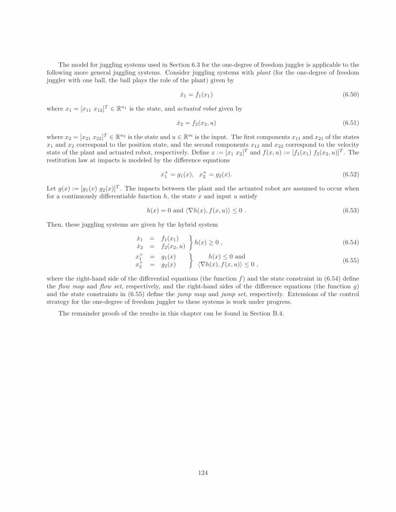
The model for juggling systems used in Section 6.3 for the one-degree of freedom juggler is applicable to thefollowing more general juggling systems. Consider juggling systems with plant (for the one-degree of freedomjuggler with one ball, the ball plays the role of the plant) given by

x1 = f1(x1) (6.50)

where x1 = [x11 x12]T ∈ R

n1 is the state, and actuated robot given by

x2 = f2(x2, u) (6.51)

where x2 = [x21 x22]T ∈ R

n2 is the state and u ∈ Rm is the input. The first components x11 and x21 of the states

x1 and x2 correspond to the position state, and the second components x12 and x22 correspond to the velocitystate of the plant and actuated robot, respectively. Define x := [x1 x2]

T and f(x, u) := [f1(x1) f2(x2, u)]T . The

restitution law at impacts is modeled by the difference equations

x+1 = g1(x), x+

2 = g2(x). (6.52)

Let g(x) := [g1(x) g2(x)]T . The impacts between the plant and the actuated robot are assumed to occur when

for a continuously differentiable function h, the state x and input u satisfy

h(x) = 0 and 〈∇h(x), f(x, u)〉 ≤ 0 . (6.53)

Then, these juggling systems are given by the hybrid system

x1 = f1(x1)x2 = f2(x2, u)

h(x) ≥ 0 , (6.54)

x+1 = g1(x)x+

2 = g2(x)

h(x) ≤ 0 and

〈∇h(x), f(x, u)〉 ≤ 0 ,(6.55)

where the right-hand side of the differential equations (the function f) and the state constraint in (6.54) definethe flow map and flow set, respectively, and the right-hand sides of the difference equations (the function g)and the state constraints in (6.55) define the jump map and jump set, respectively. Extensions of the controlstrategy for the one-degree of freedom juggler to these systems is work under progress.

The remainder proofs of the results in this chapter can be found in Section B.4.

124

Chapter 7

Simulation Theory

7.1 Introduction

The theory of numerical simulation for differential equations is well-developed and several textbooks in thesubject are available. The properties of integration schemes for differential equations are generally studied asdynamical systems. The analysis of stability and convergence of one-step integration schemes (like Euler andRunge-Kutta), multi-step algorithms (like Adams method and backward differentiation), and their variable stepversions establishes conditions on the step size for integration and on the discrete map used to approximatethe solutions of the system so that the simulations are close to the actual solutions. The ultimate goal in thesenumerical integration schemes is to reproduce with arbitrary precision the trajectories to the mathematicalmodel under simulation. In other words, it is desired that the simulated solutions are close to the solutions tothe actual model, and that this level of closeness can be adjusted with the integration step size of the numericalsolver. Moreover, it is also desired that when the dynamical system to be simulated has an asymptoticallystable set, the simulated model preserves that asymptotic stability in a practical sense. Results of this type,though currently not available for hybrid systems, can be found for differential equations and inclusions in thenumerical analysis literature.

In this chapter, a hybrid simulator model for hybrid systems H is proposed. Conditions on the data of thehybrid simulator are established to show the following sequence of results:

1) On compact hybrid time domains, every simulation to a hybrid system is arbitrarily close to a solution ofthe hybrid system;

2) Asymptotically stable compact sets for a hybrid system are semiglobally practically asymptotically stablecompact sets for the hybrid simulator;

3) Asymptotically stable compact sets for the hybrid simulator are continuous in the step size s.

These conditions basically consist of a closeness property for the integration scheme that is used to simulate theflows of the hybrid system, plus additional conditions on inflations of the jump mapping and the jump and flowsets. To generate these results, jumps are not assumed to be “forced” when the trajectories hit the boundaryof the jump set, sometimes considered as forcing or triggering semantics. Alternatively, trajectories are allowedto “enter” the jump set, sometimes referred to as enabling semantics.

125

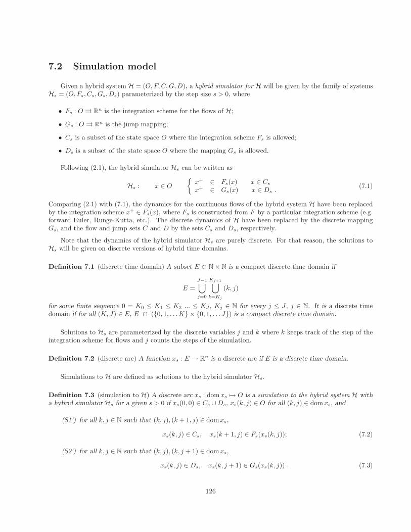
7.2 Simulation model

Given a hybrid system H = (O,F,C,G,D), a hybrid simulator for H will be given by the family of systemsHs = (O,Fs, Cs, Gs, Ds) parameterized by the step size s > 0, where

• Fs : O →→ Rn is the integration scheme for the flows of H;

• Gs : O →→ Rn is the jump mapping;

• Cs is a subset of the state space O where the integration scheme Fs is allowed;

• Ds is a subset of the state space O where the mapping Gs is allowed.

Following (2.1), the hybrid simulator Hs can be written as

Hs : x ∈ O

x+ ∈ Fs(x) x ∈ Cs

x+ ∈ Gs(x) x ∈ Ds .(7.1)

Comparing (2.1) with (7.1), the dynamics for the continuous flows of the hybrid system H have been replacedby the integration scheme x+ ∈ Fs(x), where Fs is constructed from F by a particular integration scheme (e.g.forward Euler, Runge-Kutta, etc.). The discrete dynamics of H have been replaced by the discrete mappingGs, and the flow and jump sets C and D by the sets Cs and Ds, respectively.

Note that the dynamics of the hybrid simulator Hs are purely discrete. For that reason, the solutions toHs will be given on discrete versions of hybrid time domains.

Definition 7.1 (discrete time domain) A subset E ⊂ N × N is a compact discrete time domain if

E =J−1⋃

j=0

Kj+1⋃

k=Kj

(k, j)

for some finite sequence 0 = K0 ≤ K1 ≤ K2 ... ≤ KJ , Kj ∈ N for every j ≤ J , j ∈ N. It is a discrete timedomain if for all (K, J) ∈ E, E ∩ (0, 1, . . .K × 0, 1, . . . J) is a compact discrete time domain.

Solutions to Hs are parameterized by the discrete variables j and k where k keeps track of the step of theintegration scheme for flows and j counts the steps of the simulation.

Definition 7.2 (discrete arc) A function xs : E → Rn is a discrete arc if E is a discrete time domain.

Simulations to H are defined as solutions to the hybrid simulator Hs.

Definition 7.3 (simulation to H) A discrete arc xs : domxs 7→ O is a simulation to the hybrid system H witha hybrid simulator Hs for a given s > 0 if xs(0, 0) ∈ Cs ∪Ds, xs(k, j) ∈ O for all (k, j) ∈ domxs, and

(S1’) for all k, j ∈ N such that (k, j), (k + 1, j) ∈ domxs,

xs(k, j) ∈ Cs, xs(k + 1, j) ∈ Fs(xs(k, j)); (7.2)

(S2’) for all k, j ∈ N such that (k, j), (k, j + 1) ∈ domxs,

xs(k, j) ∈ Ds, xs(k, j + 1) ∈ Gs(xs(k, j)) . (7.3)

126

0

2

4

6

0 1 2 3 4 5 6 7

0

1

2

3

4

5

6

7

8

j [jumps]

t [ordinary time]

x 1 [m]

0

2

4

6

0 1 2 3 4 5 6 7

0

1

2

3

4

5

6

7

8

j [jumps]

t [ordinary time]

x 1 [m]

Figure 7.1. Solution and simulation to the bouncing ball model: (a) Solution for initial conditions x1(0, 0) =6m, x2(0, 0) = 0.1m/s, constants g = 9.8m/s2, γ = 0.6; position x1 and hybrid time domain are plotted; (b)Simulation to the bouncing ball model with step size s = 0.1sec, initial conditions x1(0, 0) = 6m, x2(0, 0) =0.1m/s, and constants g = 9.8m/s2, γ = 0.6; discrete arc xs denoted with +, hybrid arc ξs denoted with −−,and discrete domain denoted with ∗.

One way to translate a simulation xs on the discrete time domain domxs to a hybrid arc ξs on a hybridtime domain dom ξs is by piecewise linear interpolation of the flows:

• for every (t, j) such that (k, j), (k + 1, j) ∈ domxs, ks ≤ t ≤ (k + 1)s,

ξs(t, j) = xs(k, j) + 1s (t− ks)(xs(k + 1, j) − xs(k, j)),

tj = ks, tj+1 = (k + 1)s;(7.4)

• for every (t, j) such that (k, j), (k, j + 1) ∈ domxs, t = ks,

ξs(t, j) = xs(k, j), tj = tj+1 = ks; (7.5)

• J = sup(k,j)∈dom xsj and the hybrid time domain dom ξs is the union of a finite or infinite sequence of

intervals [tj , tj+1] × j, j ∈ 0, 1, . . . , J with the “last” interval possibly of the form [tj ,+∞) × j..

To illustrate the transformation of a simulation xs into a hybrid arc ξs, consider the model for a bouncingball. A solution x starting at x1(0, 0), x2(0, 0) > 0 on a hybrid time domain is depicted in Figure 7.1(a).Taking s = 0.2sec and using the forward Euler scheme for the flows, a simulation xs to the bouncing ball withxs(0, 0) = x(0, 0) and its discrete domain are shown in Figure 7.1(b) along with its respective hybrid arc ξs.

7.3 From hybrid to discrete

The hybrid simulator model proposed above suggests a discretization of the data of H. Such operationhas to be done so that the solutions of the simulator Hs and of the hybrid system H are “close” on compacthybrid time domains defined by the simulation horizon. The following assumption establishes conditions on(O,Fs, Cs, Gs, Ds) in terms of (O,F,C,G,D) for that purpose.

127

Below, given a sequence of sets Si∞i=1, each Si subset of Rn, its outer limit, denoted by lim supi→∞ Si, is

the set of all points x ∈ Rn for which there exists a subsequence Sik

∞k=1 and points xik∈ Sik

, k = 1, 2, . . .such that xik

→ x.

Assumption 7.4 (hybrid simulator data) The data of the hybrid simulator Hs = (O,Fs, Cs, Gs, Ds) for thehybrid system H = (O,F,C,G,D) satisfies

(R1) Fs implements a specific integration algorithm and is such that, for each compact set K ⊂ O, there existsρ ∈ K∞ such that for each x ∈ Cs ∩ K and each s > 0

Fs(x) ⊂ x+ sρ(s)B + scoF (x+ ρ(s)B);

(R2) Gs is such that G0(x) ⊂ G(x) where G0 is the outer graphical limit of Gsi, for any si ց 0;

(R3) Cs and Ds are such that for any sequence si ց 0,

(lim sup

i→∞Csi

)∩O ⊂ C,

(lim sup

i→∞Dsi

)∩O ⊂ D

where lim supi→∞ Csiand lim supi→∞Dsi

are the outer limits of the sequence of sets Csiand Dsi

, re-spectively.

Assumption (R1) is a condition on the integrator scheme for flows. It implies that, given a compact set K ⊂ Rn,

at every point in Cs ∩K where the integration scheme is active, the new value is close to a perturbed solution tox ∈ F (x). When simulating a hybrid system, the projection function is required since there is no guarantee thatthe integration step s keeps the simulations in Cs ∪Ds, even if it keeps them in O. For Assumption (R2) recallthat G0 is the outer graphical limit of Gsi

when gph G0 = lim supi→∞ gph Gsiand Gsi

is locally eventuallybounded with respect to O (for a definition of locally eventually bounded, see Section 3.4). Assumption (R3) isa condition on the inflation by s of the flow and jump sets. Both conditions (R2) and (R3) are satisfied whenGs, Cs, and Ds are outer perturbations of G,C, and D, respectively. More precisely, given a continuous functionα : O → R≥0 such that, for all x ∈ O, x + α(x)B ⊂ O, the outer perturbation of G,C, and D for δ ∈ (0, 1) isgiven by the set-valued mapping Gδ and sets Cδ, Dδ defined by

Gδ := y | y ∈ η + δα(η)B, η ∈ G(x + δα(x)B)Cδ := x ∈ O | (x+ δα(x)B) ∩ C 6= ∅Dδ := x ∈ O | (x+ δα(x)B) ∩D 6= ∅

which satisfy (R2)-(R3). However, very often, when simulating hybrid systems the jump mapping G and thesets C and D are such that it is sufficient to choose Gs ≡ G, Cs = C, and Ds = D (this is a reasonable situationwhen G, C, and D are known precisely).

Example 7.5 (forward Euler method) The simplest numerical method to approximate solutions to differentialequations/inclusions is the forward Euler rule. This method is based on the first-order Taylor’s expansion ofthe continuous right-hand side around x ∈ R

n and is given by

FEs (x) = x+ sF (x) .

Condition (R1) is automatically satisfied.

128

Example 7.6 (p-stage Runge-Kutta consistent methods) For differential inclusions (or equations) x ∈ F (x)with locally bounded F : R

n →→ Rn, the update law for p-stage Runge-Kutta integration schemes, p ≥ 1, is given

by

FRKs (x) = x+ s

p∑

i=1

biξi (7.6)

where bi ∈ R and ξi ∈ F (Yi), i ∈ I := 1, 2, . . . , p. The variables Yi are called stage variables and are given by

Yi = x+ s

p∑

j=1

aijξj , ξj ∈ F (Yj) (7.7)

where aij ∈ R, (i, j) ∈ I × I. (When aij = 0 for all j ≥ i, the method is called explicit since the stage variablescan be solved without recursion.)

Provided that the equations (7.7) are solvable, either in a explicit or implicit manner, for every compact setK ⊂ R

n there exists ρ ∈ K∞ such that the stage variables satisfy

Yi ∈ x+ sρ(s) ∀i ∈ I .

Moreover, when the Runge-Kutta method is consistent, the coefficients bi satisfy

p∑

i=1

bi = 1 . (7.8)

Then, the sum in (7.6) corresponds to a convex hull condition and Assumption (R1) is satisfied since

FRKs (x) ⊂ x+ s co

i∈IF (Yi) ⊂ x+ s coF (x+ ρ(s)) .

7.4 Closeness and continuity properties

The hybrid simulator Hs = (O,Fs, Cs, Gs, Ds) is considered as a perturbation of the hybrid system H =(O,F,C,G,D). The following result exploits this idea to show that for a given simulation horizon (T, J), bya proper choice of the step size, every simulation to the hybrid system is close in the graphical sense to somesolution of the hybrid system with a desired level of closeness.

Theorem 7.7 (closeness on compact domains) Assume that H satisfies the hybrid basic conditions and that,for some compact set K ⊂ O, it is forward complete at every x0 ∈ K. Assume that the family of hybrid systemsHs satisfies Assumption 7.4. Then, for any ε > 0 and any simulation horizon (T, J) ∈ R≥0×N there exists s∗ > 0with the following property: for any s ∈ (0, s∗] and any simulation xs to Hs with xs(0, 0) = x0

s ∈ (K + εB) ∩Othere exists a solution x to H with x(0, 0) ∈ K such that for all (k, j) ∈ domxs with ks ≤ T , j ≤ J , there existsm such that (m, j) ∈ domx, |ks−m| ≤ ε, and

|xs(k, j) − x(m, j)| ≤ ε . (7.9)

Proof. Let ε > 0 and a simulation horizon (T, J) ∈ R≥0 × N be given. Let reachHs

(T,J)(K) be the finite-time

(up to (T, J)) reachable set of Hs from the compact set K, i.e.,

reachHs

(T,J)(K) := xs(k, j)|xs is a simulation to H, xs(0, 0) ∈ K, (k, j) ∈ domxs, ks ≤ T, j ≤ J .

129

By Definition 7.3, any simulation xs : domxs → O to H, domxs ⊂ [0, T ] × 0, . . . , J, satisfies (S1s) and(S2s), and can be extended to a hybrid arc ξs : dom ξs → O on a hybrid time domain dom ξs constructed as in(7.4)-(7.5). Note that for each (t, j) ∈ dom ξs such that (k, j), (k + 1, j) ∈ dom ξs, ks ≤ t ≤ (k + 1)s, by (R1) inAssumption 7.4 we have that

|ξs(ks, j) − ξs(t, j)| ≤ |xs(k, j) − xs(k + 1, j)| ≤ sδ′(s) (7.10)

whereδ′(s) := max

η∈ reachHs(T,J)(K)∩Cs

coF ((η + ρ(s)B) ∩O) + ρ(s)B .

Then, using (R1) in Assumption 7.4 and (7.10), for every (t, j) ∈ dom ξs so that (k, j), (k + 1, j) ∈ domxs,ks ≤ t ≤ (k + 1)s, ξs satisfies

ξs(t, j) =xs(k + 1, j) − xs(k, j)

s∈ coF ((ξs(ks, j) + ρ(s)B) ∩O) + ρ(s)B

⇒ ξs(t, j) ∈ coF ((ξs(t, j) + (sδ′(s) + ρ(s))B) ∩O) + (sδ′(s) + ρ(s))B

and

ξs(t, j) ∈x ∈ O

∣∣ (x + sδ′(s)B) ∩ Cs 6= ∅.

By construction of ξs, for every (t, j) so that (k, j), (k, j + 1) ∈ domxs, t = ks,

ξs(t, j) ∈ Ds, ξs(t, j + 1) ∈ Gs(ξs(t, j)) .

Given δ > 0 pick s > 0 such that sδ′(s) + ρ(s) ≤ δ. Define

Fδ(x) := coF ((x + δB) ∩O) + δB, Gδ(x) := Gs(δ)(x),

Cδ :=x ∈ O

∣∣ (x+ δB) ∩ Cs(δ) 6= ∅, Dδ := Ds(δ)

where the dependence of s on δ is explicitly indicated. In fact, s approaches zero as δ → 0.

From the properties of ξs above, hybrid arcs ξs obtained from simulations xs to H are solutions to theperturbed hybrid system Hδ := (O,Fδ , Cδ, Gδ, Dδ). For any arbitrary sequence δi∞i=1 with 1 > δ1 > δ2 >. . . > 0 converging to zero, sequences Ci = Cδi

, Di = Dδi, Fi = Fδi

, Gi = Gδisatisfy assumptions (C1), (C2),

(C3), and (C4) in [39, Section 5]. Assumption 7.4 automatically implies that Ci, Di, and Gi satisfy (C1), (C2),(C3), and (C4). The proof that Fi satisfies (C2) and (C3) can be found in Lemma 5.4 in [39] which follows bythe fact that Fi is an outer perturbation of F .

It follows that using the techniques in [22], a version of Corollary 5.5 in [39] without completeness as-sumptions holds. Then, given ε > 0 there exists δ∗ > 0 such that for each δ ∈ (0, δ∗], each s > 0 such thatsδ′(s)+ρ(s) ≤ δ, and each solution to Hδ starting from K+ δB, in particular, every hybrid arc ξs obtained froma simulation xs, domxs ⊂ [0, T ]×0, . . . , J, there exists a solution x to H with x(0, 0) ∈ K such that for every(k, j) ∈ domxs with ks ≤ T , j ≤ J , there existsm such that (m, j) ∈ domx, |ks−m| ≤ ε, |xs(k, j)−x(m, j)| ≤ ε.To finish the proof, let s∗ > 0 be the maximum s satisfying sδ′(s) + ρ(s) ≤ δ∗.

When a hybrid system H has an asymptotically stable compact set A, the hybrid simulator Hs has thesame set semiglobally practically asymptotically stable.

Theorem 7.8 (practical semiglobal stability of simulations) Suppose that H = (O,F,C,G,D) satisfies thehybrid basic conditions and that A is an asymptotically stable compact set with basin of attraction BA open

130

relative to C ∪ D. Let U ⊂ O be any open set such that BA = (C ∪ D) ∩ U . Assume that the family ofhybrid systems Hs = (O,Fs, Cs, Gs, Ds) satisfies Assumption 7.4. Then, the set A is semiglobally practicallyasymptotically stable for Hs, i.e., for each proper indicator ω : U → R≥0 of A with respect to U , each compactset K ⊂ BA, and each ε > 0 there exists β ∈ KLL and s∗ > 0 such that for each s ∈ (0, s∗] every simulation xs

to H starting from K satisfies, for each (k, j) ∈ domxs,

ω(xs(k, j)) ≤ β(ω(xs(0, 0)), ks, j) + ε . (7.11)

Proof. It follows that using the techniques in [22], a version of Theorem B.14 without completeness assumptionsholds. Then, for each proper indicator ω : U → R≥0 of A with respect to U there exists β ∈ KLL such that foreach solution x to H with x(0, 0) ∈ BA, for all (t, j) ∈ domx,

ω(x(t, j)) ≤ β(ω(x(0, 0)), t, j) .

By Assumption 7.4, we proceed as in Theorem 7.7 to construct a perturbed hybrid system Hδ such that everyhybrid arc ξs obtained from a simulation xs to H is a solution to it. By construction, Hδ satisfies (C1), (C2),(C3), and (C4) in [39, Section 5]. Then, by Theorem B.15, for each compact set K ⊂ BA and each ε > 0 thereexists δ∗ > 0 such that for each δ ∈ (0, δ∗], s > 0 such that sδ′(s) + ρ(s) ≤ δ, every hybrid arc ξs obtained froma simulation xs starting from K satisfies, for all (t, j) ∈ dom ξs,

ω(ξs(t, j)) ≤ β(ω(ξs(0, 0)), t, j) + ε .

Let s∗ > 0 be the largest s that satisfies sδ′(s) + ρ(s) ≤ δ. Hence, by the construction of ξs from xs, (7.11)holds.

Theorem 7.8 implies that simulations starting from K with unbounded discrete time domain approach thecompact set Aε := x ∈ O | ω(x) ≤ ε. This property holds for small enough step size s. Clearly, as the desiredlevel of closeness to A which is given by ε decreases, the required step size s decreases as well.

In order to guarantee that simulations exist for arbitrarily large simulation horizon as required in thedefinition of asymptotic stability in Definition 4.1, we strengthen assumptions (R1) and (R2) in Assumption 7.4as follows.

Assumption 7.9 (conditions on Hs for completeness)

The data of the hybrid simulator Hs = (O,Fs, Cs, Gs, Ds) for the hybrid system H = (O,F,C,G,D) satisfiesthe following conditions: for each compact set K ⊂ O there exists s∗ > 0 such that for all s ∈ (0, s∗]

(R1c) Fs(Cs ∩K) ⊂ Cs ∪Ds and for each x ∈ Cs ∩K, Fs(x) 6= ∅;

(R2c) Gs(Ds ∩K) ⊂ Cs ∪Ds and for each x ∈ Ds ∩K, Gs(x) 6= ∅.

Theorem 7.10 (continuity of asymptotically stable sets) Let Assumption 7.4 and 7.9 hold. Suppose that thehybrid system H = (O,F,C,G,D) satisfies the hybrid basic conditions and that A is an asymptotically stablecompact set with basin of attraction BA which is open relative to C ∪D. Then, there exists s∗ such that for alls ∈ (0, s∗], the hybrid simulator Hs has an asymptotically stable set As which satisfies

dH(As,A) → 0 as sց 0 . (7.12)

Proof. Let K be any compact set such that for some ε∗ > 0, A+ ε∗B ⊂ K ⊂ O. Let β ∈ KLL and s∗ > 0 comefrom Theorem 7.8 with K, ε ∈ (0, ε∗], and ω(·) = | · |A. Using Assumption 7.9, redefine s∗ above so that (R1c)

131

and (R2c) hold. Then, every simulation to H starting from K exists for arbitrarily large simulation horizon(T, J).

By Assumption 7.4, we proceed as in Theorem 7.7 to construct a perturbed hybrid system Hδ such thatevery hybrid arc ξs obtained from a simulation xs to H is a solution to it. By construction, Hδ satisfies (C1),(C2), (C3), and (C4) in [39, Section 5]. Let

Bε := reachHδ (A + 2εB)

where reachHδ(A + 2εB) is the reachable set of Hδ from A + 2εB, i.e.,

reachHδ(A + 2εB) := ξ(t, j) | ξ is a solution to ∈ Hδ, ξs(0, 0) ∈ (A + 2εB) .

By Theorem 7.8, Bε is bounded. Since Bε is closed by definition, it follows that it is compact. We now showthat it is forward invariant. Let ξ0 ∈ Bε and let ξ be a solution to Hδ from ξ0. Suppose that there exists(t′, j′) ∈ dom ξ for which ξ(t′, j′) 6∈ Bε. By definition of Bε, since ξ0 ∈ Bε, the solution ξ belongs to Bε for all(t, j) ∈ dom ξ. This is a contradiction. Then, Bε is forward invariant. To show that solutions to Hδ startingfrom K converge to Bε uniformly, note that, Theorem 7.8 implies that there exists N > 0 such that for everysolution ξ to Hδ with ξ(0, 0) ∈ K, we have

|ξ(t, j)|A ≤ β(|ξ(0, 0)|A, t, j) + ε ≤ 2ε (7.13)

for all (t, j) ∈ dom ξ, t + j ≥ N , for large enough simulation horizon. Then, since Bε is compact, forwardinvariant, and uniformly attractive from K, by Proposition 6.2 in [39], Bε is an asymptotically stable set forHδ. Hence, it is an asymptotically stable set for Hs.

Finally, note that B0 = reachHδ (A) = A and that as ε ց 0, dH(Bε, B0) → 0. Then, since ε and s arerelated through Theorem 7.8 and are such that s ց 0 as ε ց 0, with some abuse of notation, the claim holdswith As = Bε.

7.4.1 Numerical example

Consider the bouncing ball example in Section 2.2.1 with regular data which, for convenience, is rewrittenbelow:

O := R2, f(x) :=

[x2

−g

], C :=

x ∈ R

2 | x1 ≥ 0

(7.14)

g(x) :=

[x1

−λx2

], D :=

x ∈ R

2 | x1 = 0 , x2 ≤ 0

(7.15)

where g > 0 is the gravity constant and λ ∈ [0, 1) is the restitution coefficient. Denote this system by HBB.

A hybrid simulator for the bouncing ball system is given by

fs(x) = x+ sf(x), Cs = C,gs(x) = g(x), Ds = x ∈ O | −α(s)|x2| ≤ x1 ≤ 0, x2 ,

where s > 0 is the integration step for the integration scheme for flows and α : R≥0 → R≥0 is a continuousfunction satisfying α(s) > s for all s > 0, α(0) = 0. Note that Hs = (O, fs, Cs, gs, Ds) satisfies Assumption 7.4.Note that one of the perturbations included is due to the integration scheme for the flows which is implemented asa forward Euler rule. Moreover, the jump setD is perturbed in order to satisfy Assumption 7.9 and consequently,guarantee that simulations to the bouncing ball starting in C ∪D exist for all simulation horizon.

132

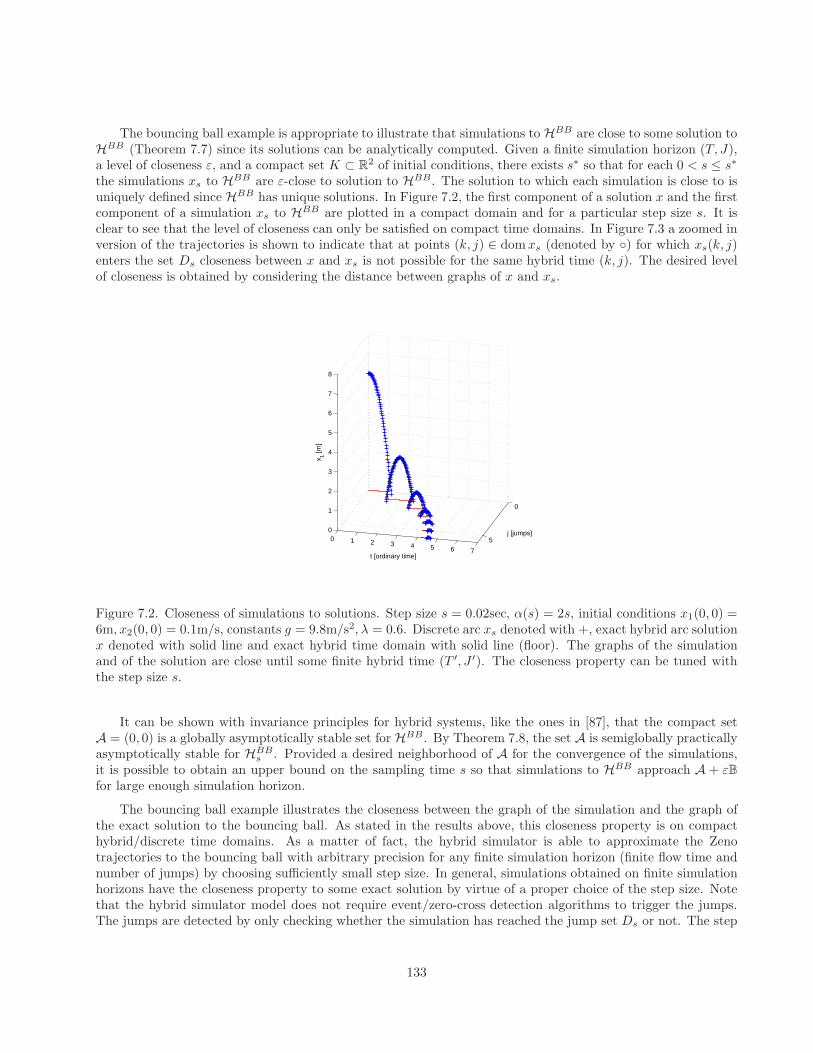
The bouncing ball example is appropriate to illustrate that simulations to HBB are close to some solution toHBB (Theorem 7.7) since its solutions can be analytically computed. Given a finite simulation horizon (T, J),a level of closeness ε, and a compact set K ⊂ R

2 of initial conditions, there exists s∗ so that for each 0 < s ≤ s∗

the simulations xs to HBB are ε-close to solution to HBB. The solution to which each simulation is close to isuniquely defined since HBB has unique solutions. In Figure 7.2, the first component of a solution x and the firstcomponent of a simulation xs to HBB are plotted in a compact domain and for a particular step size s. It isclear to see that the level of closeness can only be satisfied on compact time domains. In Figure 7.3 a zoomed inversion of the trajectories is shown to indicate that at points (k, j) ∈ domxs (denoted by ) for which xs(k, j)enters the set Ds closeness between x and xs is not possible for the same hybrid time (k, j). The desired levelof closeness is obtained by considering the distance between graphs of x and xs.

0

50 1 2 3 4 5 6 7

0

1

2

3

4

5

6

7

8

j [jumps]

t [ordinary time]

x 1 [m]

Figure 7.2. Closeness of simulations to solutions. Step size s = 0.02sec, α(s) = 2s, initial conditions x1(0, 0) =6m, x2(0, 0) = 0.1m/s, constants g = 9.8m/s2, λ = 0.6. Discrete arc xs denoted with +, exact hybrid arc solutionx denoted with solid line and exact hybrid time domain with solid line (floor). The graphs of the simulationand of the solution are close until some finite hybrid time (T ′, J ′). The closeness property can be tuned withthe step size s.

It can be shown with invariance principles for hybrid systems, like the ones in [87], that the compact setA = (0, 0) is a globally asymptotically stable set for HBB. By Theorem 7.8, the set A is semiglobally practicallyasymptotically stable for HBB

s . Provided a desired neighborhood of A for the convergence of the simulations,it is possible to obtain an upper bound on the sampling time s so that simulations to HBB approach A + εBfor large enough simulation horizon.

The bouncing ball example illustrates the closeness between the graph of the simulation and the graph ofthe exact solution to the bouncing ball. As stated in the results above, this closeness property is on compacthybrid/discrete time domains. As a matter of fact, the hybrid simulator is able to approximate the Zenotrajectories to the bouncing ball with arbitrary precision for any finite simulation horizon (finite flow time andnumber of jumps) by choosing sufficiently small step size. In general, simulations obtained on finite simulationhorizons have the closeness property to some exact solution by virtue of a proper choice of the step size. Notethat the hybrid simulator model does not require event/zero-cross detection algorithms to trigger the jumps.The jumps are detected by only checking whether the simulation has reached the jump set Ds or not. The step

133

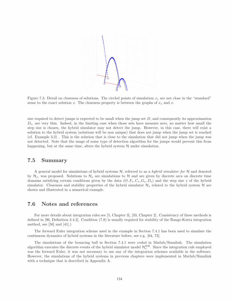
Figure 7.3. Detail on closeness of solutions. The circled points of simulation xs are not close in the “standard”sense to the exact solution x. The closeness property is between the graphs of xs and x.

size required to detect jumps is expected to be small when the jump set D, and consequently its approximationDs, are very thin. Indeed, in the limiting case when those sets have measure zero, no matter how small thestep size is chosen, the hybrid simulator may not detect the jump. However, in this case, there will exist asolution to the hybrid system (solutions will be non unique) that does not jump when the jump set is reached(cf. Example 3.3) . This is the solution that is close to the simulation that did not jump when the jump wasnot detected. Note that the usage of some type of detection algorithm for the jumps would prevent this fromhappening, but at the same time, alters the hybrid system H under simulation.

7.5 Summary

A general model for simulations of hybrid systems H, referred to as a hybrid simulator for H and denotedby Hs, was proposed. Solutions to Hs are simulations to H and are given by discrete arcs on discrete timedomains satisfying certain conditions given by the data (O,Fs, Cs, Gs, Ds) and the step size s of the hybridsimulator. Closeness and stability properties of the hybrid simulator Hs related to the hybrid system H areshown and illustrated in a numerical example.


For more details about integration rules see [5, Chapter 3], [33, Chapter 2]. Consistency of these methods isdefined in [96, Definition 3.4.2]. Condition (7.8) is usually required for stability of the Runge-Kutta integrationmethod, see [50] and [41].)

The forward Euler integration scheme used in the example in Section 7.4.1 has been used to simulate thecontinuous dynamics of hybrid systems in the literature before, see e.g. [64, 73].

The simulations of the bouncing ball in Section 7.4.1 were coded in Matlab/Simulink. The simulationalgorithm executes the discrete events of the hybrid simulator model HBB

s . Since the integration rule employedwas the forward Euler, it was not necessary to use any of the integration schemes available in the software.However, the simulations of the hybrid systems in previous chapters were implemented in Matlab/Simulinkwith a technique that is described in Appendix A.

134

Chapter 8

Conclusion

In this thesis, a dynamical systems approach to modeling, analysis, and design of hybrid systems was pursuedfrom a robust stability point of view. A summary of the contents of this document and several future researchthrusts emerging from this thesis are the focus of this chapter.

8.1 Summary

A general modeling framework for hybrid control systems was introduced in Chapter 2. Hybrid systems weremodeled by hybrid equations with a state space, a flow map (given by a single-valued function or a set-valuedmapping), a flow set, a jump map (given by a single-valued function or a set-valued mapping), and a jump set.Solutions were defined as hybrid arcs and parametrized both by flow time t and jump time j on hybrid timedomains, which are subsets of R≥0 ×N. Several examples were presented to illustrate the modeling framework.

In Chapter 3, it was shown that the robustness properties of hybrid systems are very sensitive to theproperties of the data defining the hybrid equations. Several examples illustrated the effect of this perturbationin the system behavior. Mild conditions on these objects, the hybrid basic conditions, were motivated andshown to capture the effect of arbitrarily small state perturbations in the nominal set of solutions of what wecalled a regularized hybrid system. The regularization procedure and the solutions to the resulting regularizedsystem followed the regularization and solution notion introduced by Krasovskii in [55].

Structural properties of solutions guaranteed by the hybrid basic conditions allowed the development of thestability and invariance results in Chapter 4. Stability and convergence tools for hybrid systems H presentedinclude hybrid versions of the classical Lyapunov stability theorem and of LaSalle’s invariance principle. Specialcases of these results, and more general invariance principles and their connections to detectability were alsoderived. The application of these tools were illustrated in several examples.

In Chapter 5, robustness of asymptotic stability for classes of closed-loop systems resulting from hybridcontrol was established. Results for perturbations arising from the presence of measurement noise, unmodeledsensor and actuator dynamics, control smoothing, and sample-and-hold devices were derived. These resultsguarantee that, for small enough perturbations, nominally asymptotically stable compact sets (or points) aresemiglobally practically asymptotically stable. The problem of globally stabilizing the one-link pendulum ona cart to the upright condition was used as benchmark to test the robustness properties of the hybrid controlstrategies proposed.

Several engineering control applications were studied in Chapter 6. The problem of robustness in stabiliza-

135

tion of nonlinear systems with certain topological structure was investigated. A general nonrobustness result forsuch problems and a hybrid controller featuring hysteresis were given. The hybrid control guarantees robust,global asymptotic stability. These results were illustrated in autonomous vehicle control problems like that ofsteering a vehicle to a disconnected set of points and to a target with obstacle avoidance. In a subsequentsection, a novel hybrid control strategy combining local state-feedback and open-loop laws for robust, globalstabilization of nonlinear systems was introduced. A decision-making algorithm was implemented in a hybridcontroller by combining logic variables and timers. The problem of stabilizing the trajectories to the pendubotsystem to the upright configuration was used to illustrate the design procedure and functionality. Finally, atracking control strategy for a class of juggling systems was presented and developed for the problem of jugglingmultiple balls with a single actuator. The proposed control algorithm provides finite-time practical tracking ofreference trajectories.

A general model for simulation of hybrid systems was introduced in Chapter 7. Solutions to the hybridsimulator were given by discrete arcs on discrete time domains satisfying certain conditions given by the dataand the step size of the hybrid simulator. The main properties of the hybrid simulator consist of a closenessproperty between solutions and simulations on compact time domains, and practical semiglobal asymptoticstability and upper semicontinuity of compact sets that are asymptotically stable for the original hybrid system.A numerical example about the simulation of a bouncing ball system was given.

These results are currently being compiled into a textbook on hybrid dynamical systems. Other results thatwere not included in this thesis are the hybrid control strategy for a class of nonlinear systems that renders theclosed-loop system uniformly input-to-state stable with respect to measurement noise in [92], the hybrid controlalgorithm with hysteresis for robust contact detection and force regulation of robotic manipulators in [24], andthe hybrid control methodology for the problem of commanding autonomous vehicles to locate a radiation sourceusing only measurements of the radiation strength in [68].

8.2 Future directions

The following research directions arise from the results in this thesis.

• Control of hybrid system with inputs: The stability results and invariance principles for “closed”systems (that is, systems without inputs) in Chapter 4 can be used to develop tools for analysis and designof “open” hybrid systems (that is, hybrid systems with inputs). The concept of “control-Lyapunov func-tion” and related control design methods for classical nonlinear systems can be generalized to the hybridsetting. This will lead to new tools for systematic design of hybrid and non-hybrid control algorithms forhybrid systems with inputs. The coupling between the control inputs and the flow/jump sets, which ispresent in the general input case, is one of the challenges in Lyapunov design of control laws for hybridsystems with inputs.

• Singular perturbation analysis: The results in Chapter 5 on robustness to a particular class of sin-gularly perturbed hybrid systems can be taken as the first step on the development of a general theoryon this topic, one that parallels the perturbation theory of classical nonlinear systems. This theory wouldenable the application of standard nonlinear control design techniques to hybrid systems with inputs.

• Advanced hybrid control methods for robotics and aerospace systems: The hybrid controlstrategies in Chapter 6 are applicable to other relevant problems in robotics and aerospace systems. Forinstance, the throw-and-catch strategy in Section 6.2 can be used to develop control algorithms withdecision-making capabilities and robustness for multiple autonomous vehicles. Robust algorithms for suchpurposes seem to be missing from the literature. The hybrid tracking control strategy in Section 6.3 forjuggling systems is applicable to more general mechanical systems with impacts, including walking andjumping robots.

136

• Embedded systems: The analysis of the effect of sample-and-hold devices on the robust stabilityproperties of closed-loop systems resulting from interconnecting a nonlinear system with a hybrid controllerin Section 5.3 of Chapter 5 can be specialized to different classes of embedded systems to derive minimumrates for sample-and-hold devices and software computation. These results would serve as guidelinesfor embedded system design. Moreover, the hybrid system framework introduced in this thesis is alsouseful to capture the dynamics of models of computation used in embedded computing, thus enabling theapplication of the new systematic tools to that area as well.

• Simulation: The initial efforts in Chapter 7 are an indicator that classical results in the simulation theoryof continuous-time systems can also be extended to the hybrid setting. A simulation theory for hybridsystems seems to be missing from the literature. The simulation framework introduced in Chapter 7 issuitable for its future development.

Other areas of science and engineering that would benefit from the theoretical and practical results inthis thesis include several problems in biology, especially those dealing with biological networks and mutualsynchronization. We believe this thesis contributes both to the theory and applications of hybrid controlsystems by introducing new modeling, analysis, and design tools that are useful for the control community andother related fields.

137

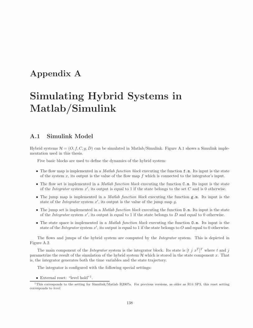
Appendix A

Simulating Hybrid Systems inMatlab/Simulink

A.1 Simulink Model

Hybrid systems H = (O, f, C, g,D) can be simulated in Matlab/Simulink. Figure A.1 shows a Simulink imple-mentation used in this thesis.

Five basic blocks are used to define the dynamics of the hybrid system:

• The flow map is implemented in a Matlab function block executing the function f.m. Its input is the stateof the system x, its output is the value of the flow map f which is connected to the integrator’s input.

• The flow set is implemented in a Matlab function block executing the function C.m. Its input is the stateof the Integrator system x′, its output is equal to 1 if the state belongs to the set C and is 0 otherwise.

• The jump map is implemented in a Matlab function block executing the function g.m. Its input is thestate of the Integrator system x′, its output is the value of the jump map g.

• The jump set is implemented in a Matlab function block executing the function D.m. Its input is the stateof the Integrator system x′, its output is equal to 1 if the state belongs to D and equal to 0 otherwise.

• The state space is implemented in a Matlab function block executing the function O.m. Its input is thestate of the Integrator system x′, its output is equal to 1 if the state belongs to O and equal to 0 otherwise.

The flows and jumps of the hybrid system are computed by the Integrator system. This is depicted inFigure A.2.

The main component of the Integrator system is the integrator block. Its state is [t j xT ]T where t and jparametrize the result of the simulation of the hybrid system H which is stored in the state component x. Thatis, the integrator generates both the time variables and the state trajectory.

The integrator is configured with the following special settings:

• External reset: “level hold”1.1This corresponds to the setting for Simulink/Matlab R2007a. For previous versions, as older as R14 SP3, this reset setting

corresponds to level.

138

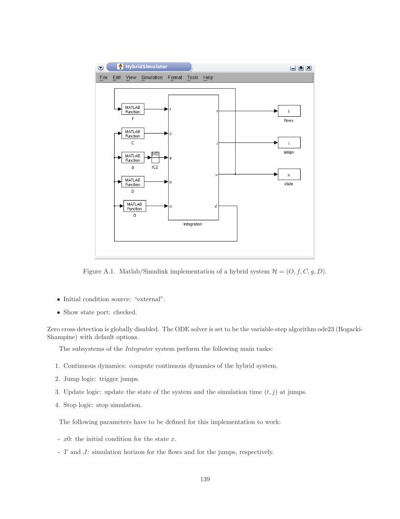
Figure A.1. Matlab/Simulink implementation of a hybrid system H = (O, f, C, g,D).

• Initial condition source: “external”.

• Show state port: checked.

Zero cross detection is globally disabled. The ODE solver is set to be the variable-step algorithm ode23 (Bogacki-Shampine) with default options.

The subsystems of the Integrator system perform the following main tasks:

1. Continuous dynamics: compute continuous dynamics of the hybrid system.

2. Jump logic: trigger jumps.

3. Update logic: update the state of the system and the simulation time (t, j) at jumps.

4. Stop logic: stop simulation.

The following parameters have to be defined for this implementation to work:

- x0: the initial condition for the state x.

- T and J : simulation horizon for the flows and for the jumps, respectively.

139

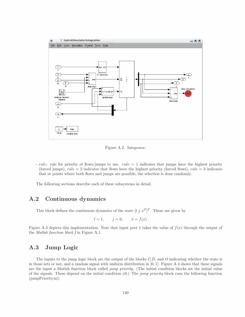
Figure A.2. Integrator.

- rule: rule for priority of flows/jumps to use. rule = 1 indicates that jumps have the highest priority(forced jumps), rule = 2 indicates that flows have the highest priority (forced flows), rule = 3 indicatesthat at points where both flows and jumps are possible, the selection is done randomly.

The following sections describe each of these subsystems in detail.

A.2 Continuous dynamics

This block defines the continuous dynamics of the state [t j xT ]T . These are given by

t = 1, j = 0, x = f(x) .

Figure A.3 depicts this implementation. Note that input port 1 takes the value of f(x) through the output ofthe Matlab function block f in Figure A.1.

A.3 Jump Logic

The inputs to the jump logic block are the output of the blocks C,D, and O indicating whether the state isin those sets or not, and a random signal with uniform distribution in [0, 1]. Figure A.4 shows that these signalsare the input a Matlab function block called jump priority. (The initial condition blocks set the initial valueof the signals. These depend on the initial condition x0.) The jump priority block runs the following function(jumpPriority.m):

140

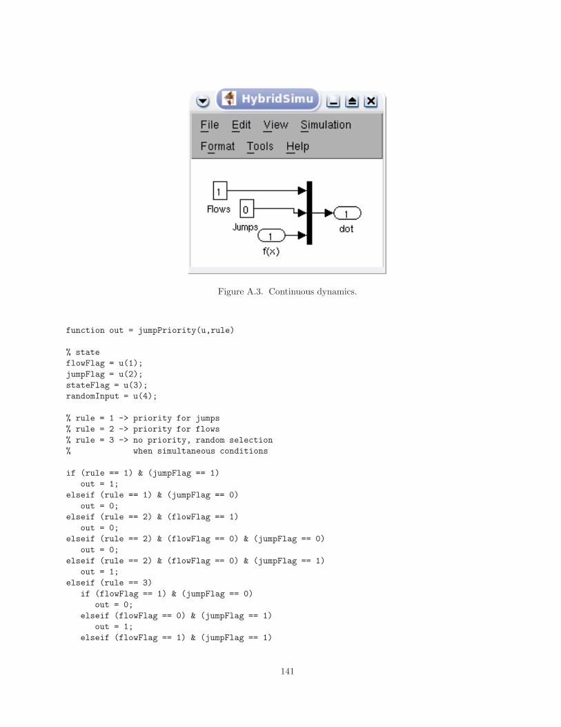
Figure A.3. Continuous dynamics.

function out = jumpPriority(u,rule)

% state

flowFlag = u(1);

jumpFlag = u(2);

stateFlag = u(3);

randomInput = u(4);

% rule = 1 -> priority for jumps

% rule = 2 -> priority for flows

% rule = 3 -> no priority, random selection

% when simultaneous conditions

if (rule == 1) & (jumpFlag == 1)

out = 1;

elseif (rule == 1) & (jumpFlag == 0)

out = 0;

elseif (rule == 2) & (flowFlag == 1)

out = 0;

elseif (rule == 2) & (flowFlag == 0) & (jumpFlag == 0)

out = 0;

elseif (rule == 2) & (flowFlag == 0) & (jumpFlag == 1)

out = 1;

elseif (rule == 3)

if (flowFlag == 1) & (jumpFlag == 0)

out = 0;

elseif (flowFlag == 0) & (jumpFlag == 1)

out = 1;

elseif (flowFlag == 1) & (jumpFlag == 1)

141

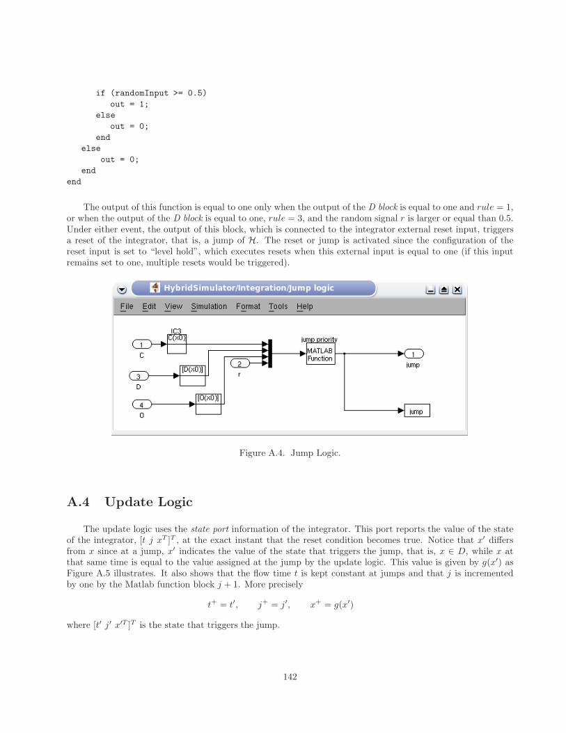
if (randomInput >= 0.5)

out = 1;

else

out = 0;

end

else

out = 0;

end

end

The output of this function is equal to one only when the output of the D block is equal to one and rule = 1,or when the output of the D block is equal to one, rule = 3, and the random signal r is larger or equal than 0.5.Under either event, the output of this block, which is connected to the integrator external reset input, triggersa reset of the integrator, that is, a jump of H. The reset or jump is activated since the configuration of thereset input is set to “level hold”, which executes resets when this external input is equal to one (if this inputremains set to one, multiple resets would be triggered).

Figure A.4. Jump Logic.

A.4 Update Logic

The update logic uses the state port information of the integrator. This port reports the value of the stateof the integrator, [t j xT ]T , at the exact instant that the reset condition becomes true. Notice that x′ differsfrom x since at a jump, x′ indicates the value of the state that triggers the jump, that is, x ∈ D, while x atthat same time is equal to the value assigned at the jump by the update logic. This value is given by g(x′) asFigure A.5 illustrates. It also shows that the flow time t is kept constant at jumps and that j is incrementedby one by the Matlab function block j + 1. More precisely

t+ = t′, j+ = j′, x+ = g(x′)

where [t′ j′ x′T ]T is the state that triggers the jump.

142

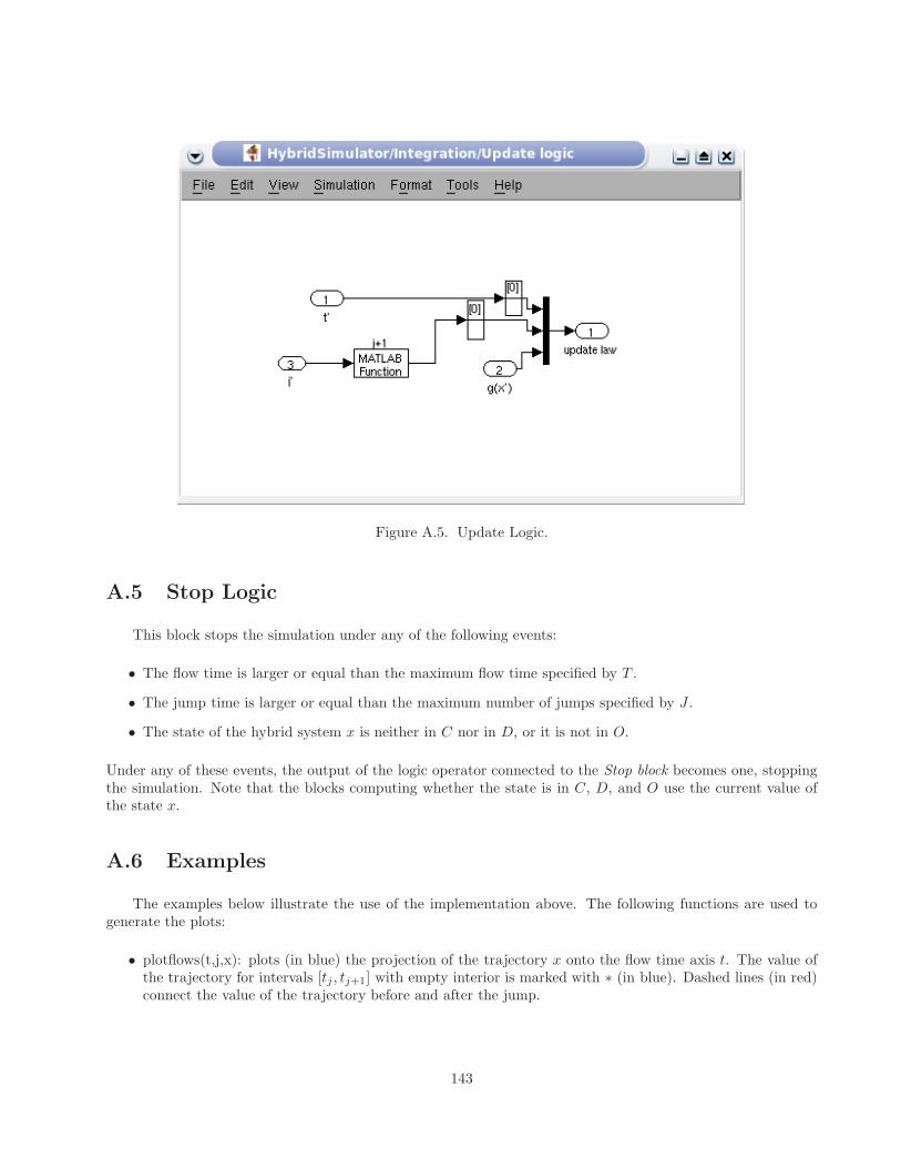
Figure A.5. Update Logic.

A.5 Stop Logic

This block stops the simulation under any of the following events:

• The flow time is larger or equal than the maximum flow time specified by T .

• The jump time is larger or equal than the maximum number of jumps specified by J .

• The state of the hybrid system x is neither in C nor in D, or it is not in O.

Under any of these events, the output of the logic operator connected to the Stop block becomes one, stoppingthe simulation. Note that the blocks computing whether the state is in C, D, and O use the current value ofthe state x.

A.6 Examples

The examples below illustrate the use of the implementation above. The following functions are used togenerate the plots:

• plotflows(t,j,x): plots (in blue) the projection of the trajectory x onto the flow time axis t. The value ofthe trajectory for intervals [tj , tj+1] with empty interior is marked with ∗ (in blue). Dashed lines (in red)connect the value of the trajectory before and after the jump.

143

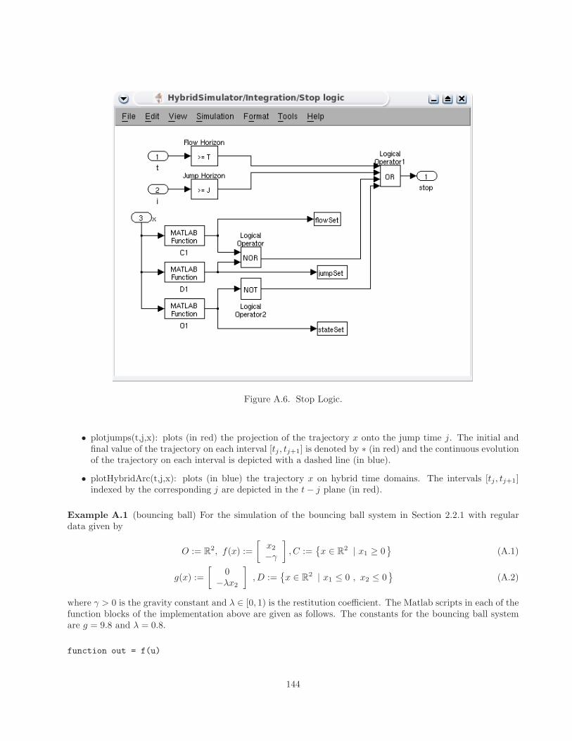
Figure A.6. Stop Logic.

• plotjumps(t,j,x): plots (in red) the projection of the trajectory x onto the jump time j. The initial andfinal value of the trajectory on each interval [tj , tj+1] is denoted by ∗ (in red) and the continuous evolutionof the trajectory on each interval is depicted with a dashed line (in blue).

• plotHybridArc(t,j,x): plots (in blue) the trajectory x on hybrid time domains. The intervals [tj , tj+1]indexed by the corresponding j are depicted in the t− j plane (in red).

Example A.1 (bouncing ball) For the simulation of the bouncing ball system in Section 2.2.1 with regulardata given by

O := R2, f(x) :=

[x2

−γ

], C :=

x ∈ R

2 | x1 ≥ 0

(A.1)

g(x) :=

[0

−λx2

], D :=

x ∈ R

2 | x1 ≤ 0 , x2 ≤ 0

(A.2)

where γ > 0 is the gravity constant and λ ∈ [0, 1) is the restitution coefficient. The Matlab scripts in each of thefunction blocks of the implementation above are given as follows. The constants for the bouncing ball systemare g = 9.8 and λ = 0.8.

function out = f(u)

144

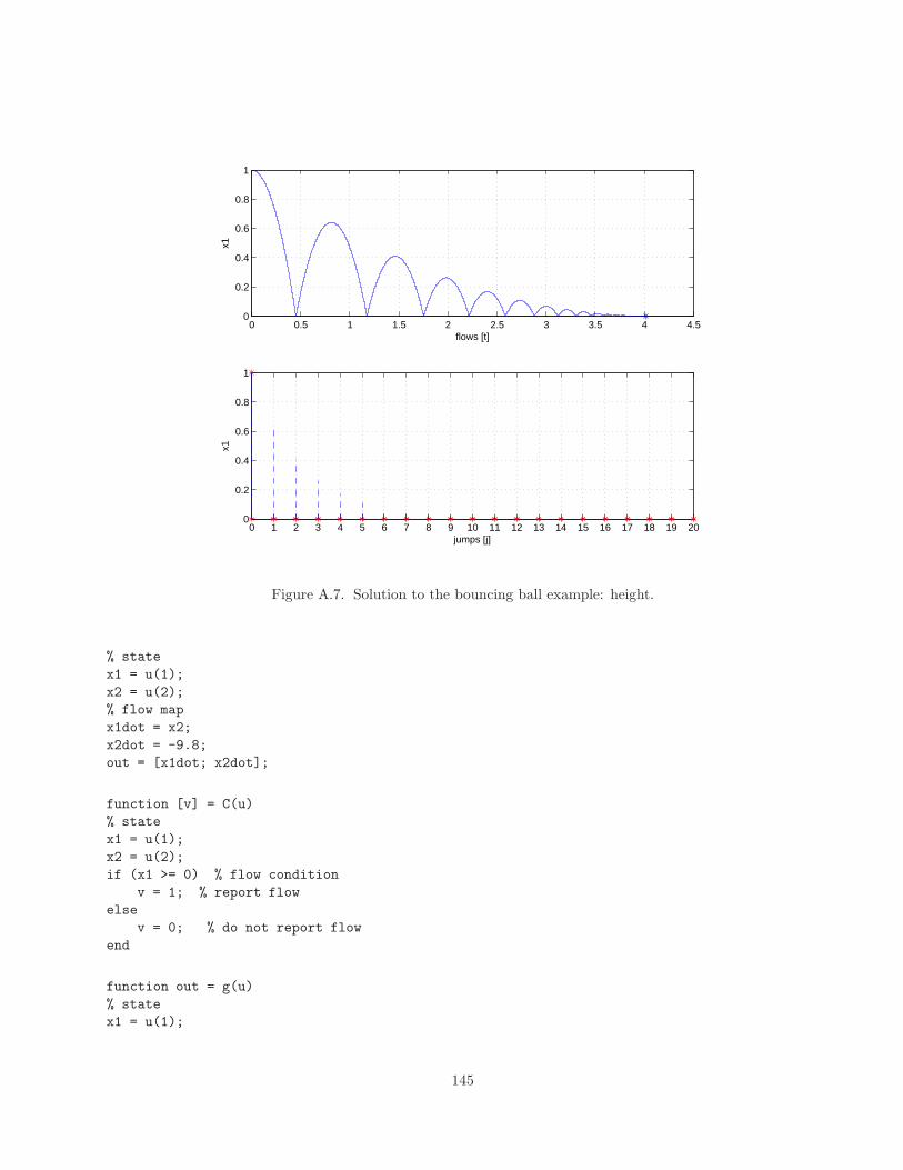
0 0.5 1 1.5 2 2.5 3 3.5 4 4.50

0.2

0.4

0.6

0.8

1

flows [t]

x1

0 1 2 3 4 5 6 7 8 9 10 11 12 13 14 15 16 17 18 19 200

0.2

0.4

0.6

0.8

1

jumps [j]

x1

Figure A.7. Solution to the bouncing ball example: height.

% state

x1 = u(1);

x2 = u(2);

% flow map

x1dot = x2;

x2dot = -9.8;

out = [x1dot; x2dot];

function [v] = C(u)

% state

x1 = u(1);

x2 = u(2);

if (x1 >= 0) % flow condition

v = 1; % report flow

else

v = 0; % do not report flow

end

function out = g(u)

% state

x1 = u(1);

145

0 0.5 1 1.5 2 2.5 3 3.5 4 4.5−6

−4

−2

0

2

4

flows [t]

x2

0 1 2 3 4 5 6 7 8 9 10 11 12 13 14 15 16 17 18 19 20−6

−4

−2

0

2

4

jumps [j]

x2

Figure A.8. Solution to the bouncing ball example: velocity.

x2 = u(2);

% jump map

x1plus = 0;

x2plus = -0.8*x2;

out = [x1plus; x2plus];

function [v] = D(u)

% state

x1 = u(1);

x2 = u(2);

if (x1 <= 0 && x2 <= 0) % jump condition

v = 1; % report jump

else

v = 0; % do not report jump

end

function [v] = O(u)

v = 1; % in the state space

A solution to the bouncing ball system from [1, 0] and with T = 10, J = 20, rule = 1, is depicted inFigure A.7 (height) and Figure A.8 (velocity). Both the projection onto t and j are shown. Figure A.9 depictsthe corresponding hybrid arc.

146

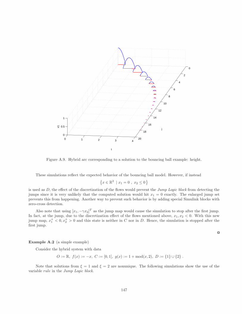
0

2

4

6

8

10

12

14

16

18

200 1 2 3 4

0

0.5

1

j

t

x1

Figure A.9. Hybrid arc corresponding to a solution to the bouncing ball example: height.

These simulations reflect the expected behavior of the bouncing ball model. However, if insteadx ∈ R

2 | x1 = 0 , x2 ≤ 0

is used as D, the effect of the discretization of the flows would prevent the Jump Logic block from detecting thejumps since it is very unlikely that the computed solution would hit x1 = 0 exactly. The enlarged jump setprevents this from happening. Another way to prevent such behavior is by adding special Simulink blocks withzero-cross detection.

Also note that using [x1,−γx2]T as the jump map would cause the simulation to stop after the first jump.

In fact, at the jump, due to the discretization effect of the flows mentioned above, x1, x2 < 0. With this newjump map, x+

1 < 0, x+2 > 0 and this state is neither in C nor in D. Hence, the simulation is stopped after the

first jump.

Example A.2 (a simple example)

Consider the hybrid system with data

O := R, f(x) := −x, C := [0, 1], g(x) := 1 + mod(x, 2), D := 1 ∪ 2 .

Note that solutions from ξ = 1 and ξ = 2 are nonunique. The following simulations show the use of thevariable rule in the Jump Logic block.

147

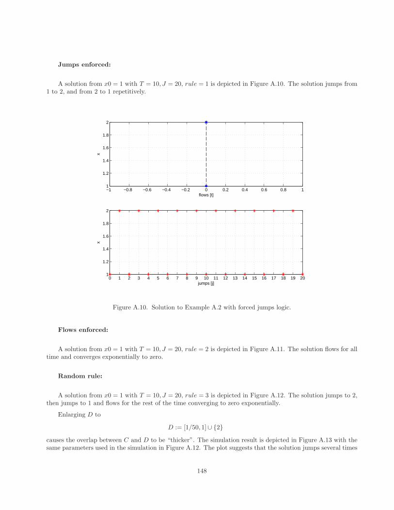
Jumps enforced:

A solution from x0 = 1 with T = 10, J = 20, rule = 1 is depicted in Figure A.10. The solution jumps from1 to 2, and from 2 to 1 repetitively.

−1 −0.8 −0.6 −0.4 −0.2 0 0.2 0.4 0.6 0.8 11

1.2

1.4

1.6

1.8

2

flows [t]

x

0 1 2 3 4 5 6 7 8 9 10 11 12 13 14 15 16 17 18 19 201

1.2

1.4

1.6

1.8

2

jumps [j]

x

Figure A.10. Solution to Example A.2 with forced jumps logic.

Flows enforced:

A solution from x0 = 1 with T = 10, J = 20, rule = 2 is depicted in Figure A.11. The solution flows for alltime and converges exponentially to zero.

Random rule:

A solution from x0 = 1 with T = 10, J = 20, rule = 3 is depicted in Figure A.12. The solution jumps to 2,then jumps to 1 and flows for the rest of the time converging to zero exponentially.

Enlarging D to

D := [1/50, 1]∪ 2

causes the overlap between C and D to be “thicker”. The simulation result is depicted in Figure A.13 with thesame parameters used in the simulation in Figure A.12. The plot suggests that the solution jumps several times

148

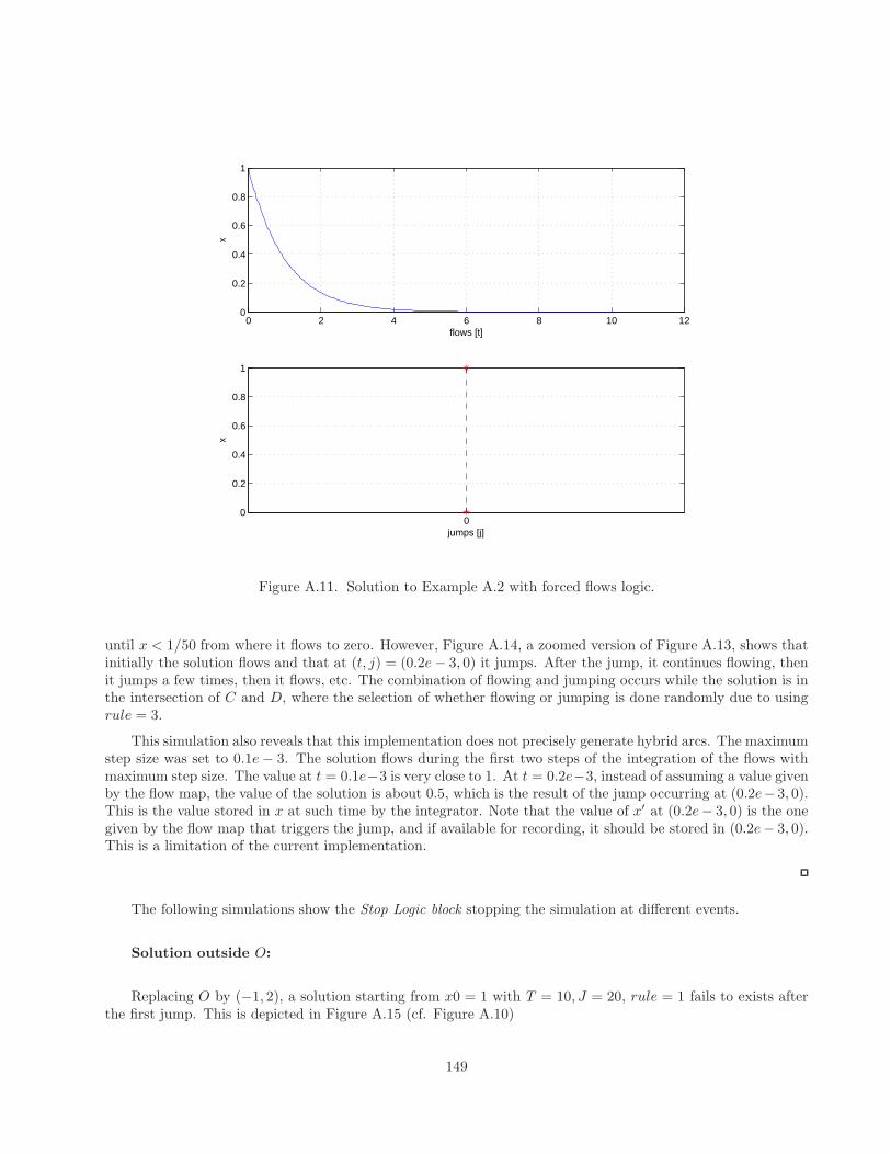
0 2 4 6 8 10 120

0.2

0.4

0.6

0.8

1

flows [t]

x

00

0.2

0.4

0.6

0.8

1

jumps [j]

x

Figure A.11. Solution to Example A.2 with forced flows logic.

until x < 1/50 from where it flows to zero. However, Figure A.14, a zoomed version of Figure A.13, shows thatinitially the solution flows and that at (t, j) = (0.2e− 3, 0) it jumps. After the jump, it continues flowing, thenit jumps a few times, then it flows, etc. The combination of flowing and jumping occurs while the solution is inthe intersection of C and D, where the selection of whether flowing or jumping is done randomly due to usingrule = 3.

This simulation also reveals that this implementation does not precisely generate hybrid arcs. The maximumstep size was set to 0.1e− 3. The solution flows during the first two steps of the integration of the flows withmaximum step size. The value at t = 0.1e−3 is very close to 1. At t = 0.2e−3, instead of assuming a value givenby the flow map, the value of the solution is about 0.5, which is the result of the jump occurring at (0.2e−3, 0).This is the value stored in x at such time by the integrator. Note that the value of x′ at (0.2e− 3, 0) is the onegiven by the flow map that triggers the jump, and if available for recording, it should be stored in (0.2e− 3, 0).This is a limitation of the current implementation.

The following simulations show the Stop Logic block stopping the simulation at different events.

Solution outside O:

Replacing O by (−1, 2), a solution starting from x0 = 1 with T = 10, J = 20, rule = 1 fails to exists afterthe first jump. This is depicted in Figure A.15 (cf. Figure A.10)

149

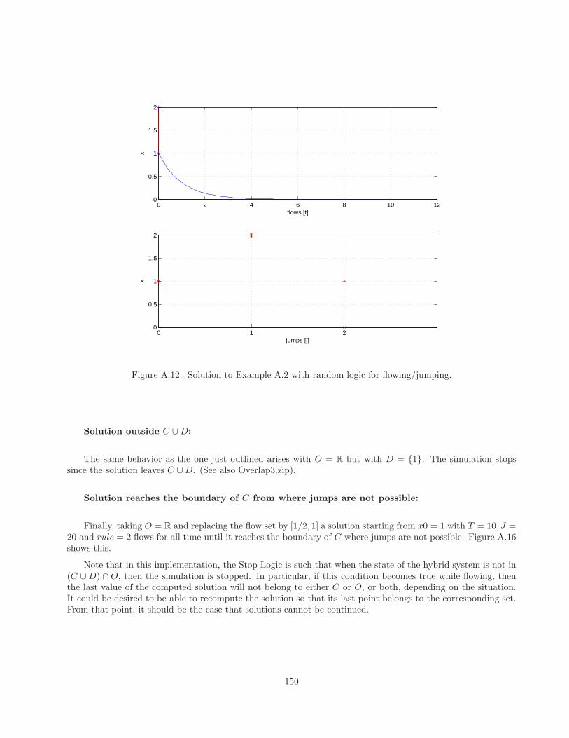
0 2 4 6 8 10 120

0.5

1

1.5

2

flows [t]

x

0 1 20

0.5

1

1.5

2

jumps [j]

x

Figure A.12. Solution to Example A.2 with random logic for flowing/jumping.

Solution outside C ∪D:

The same behavior as the one just outlined arises with O = R but with D = 1. The simulation stopssince the solution leaves C ∪D. (See also Overlap3.zip).

Solution reaches the boundary of C from where jumps are not possible:

Finally, taking O = R and replacing the flow set by [1/2, 1] a solution starting from x0 = 1 with T = 10, J =20 and rule = 2 flows for all time until it reaches the boundary of C where jumps are not possible. Figure A.16shows this.

Note that in this implementation, the Stop Logic is such that when the state of the hybrid system is not in(C ∪D) ∩ O, then the simulation is stopped. In particular, if this condition becomes true while flowing, thenthe last value of the computed solution will not belong to either C or O, or both, depending on the situation.It could be desired to be able to recompute the solution so that its last point belongs to the corresponding set.From that point, it should be the case that solutions cannot be continued.

150

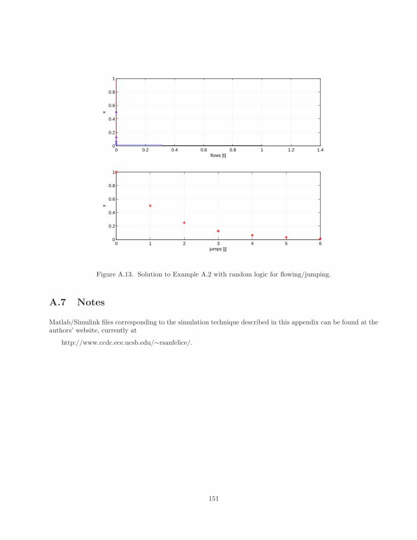
0 0.2 0.4 0.6 0.8 1 1.2 1.40

0.2

0.4

0.6

0.8

1

flows [t]

x

0 1 2 3 4 5 60

0.2

0.4

0.6

0.8

1

jumps [j]

x

Figure A.13. Solution to Example A.2 with random logic for flowing/jumping.

A.7 Notes

Matlab/Simulink files corresponding to the simulation technique described in this appendix can be found at theauthors’ website, currently at

http://www.ccdc.ece.ucsb.edu/∼rsanfelice/.

151

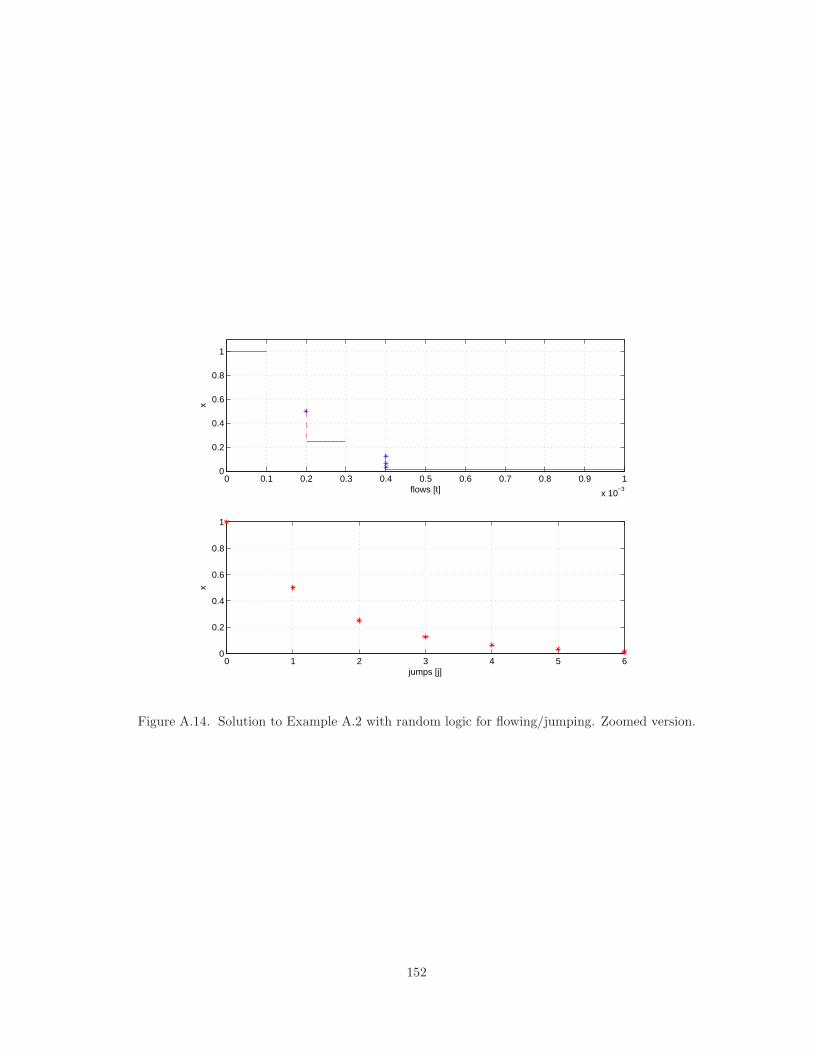
0 0.1 0.2 0.3 0.4 0.5 0.6 0.7 0.8 0.9 1

x 10−3

0

0.2

0.4

0.6

0.8

1

flows [t]

x

0 1 2 3 4 5 60

0.2

0.4

0.6

0.8

1

jumps [j]

x

Figure A.14. Solution to Example A.2 with random logic for flowing/jumping. Zoomed version.

152

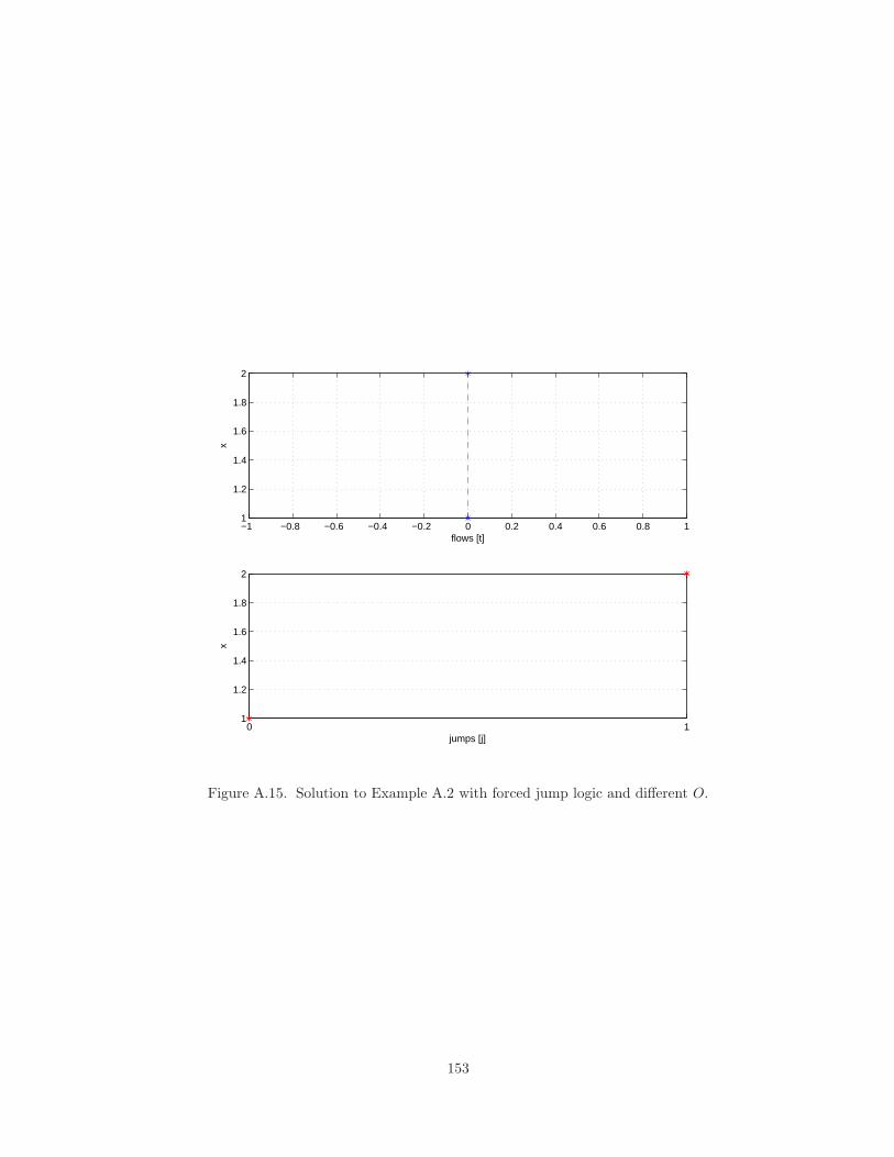
−1 −0.8 −0.6 −0.4 −0.2 0 0.2 0.4 0.6 0.8 11

1.2

1.4

1.6

1.8

2

flows [t]

x

0 11

1.2

1.4

1.6

1.8

2

jumps [j]

x

Figure A.15. Solution to Example A.2 with forced jump logic and different O.

153

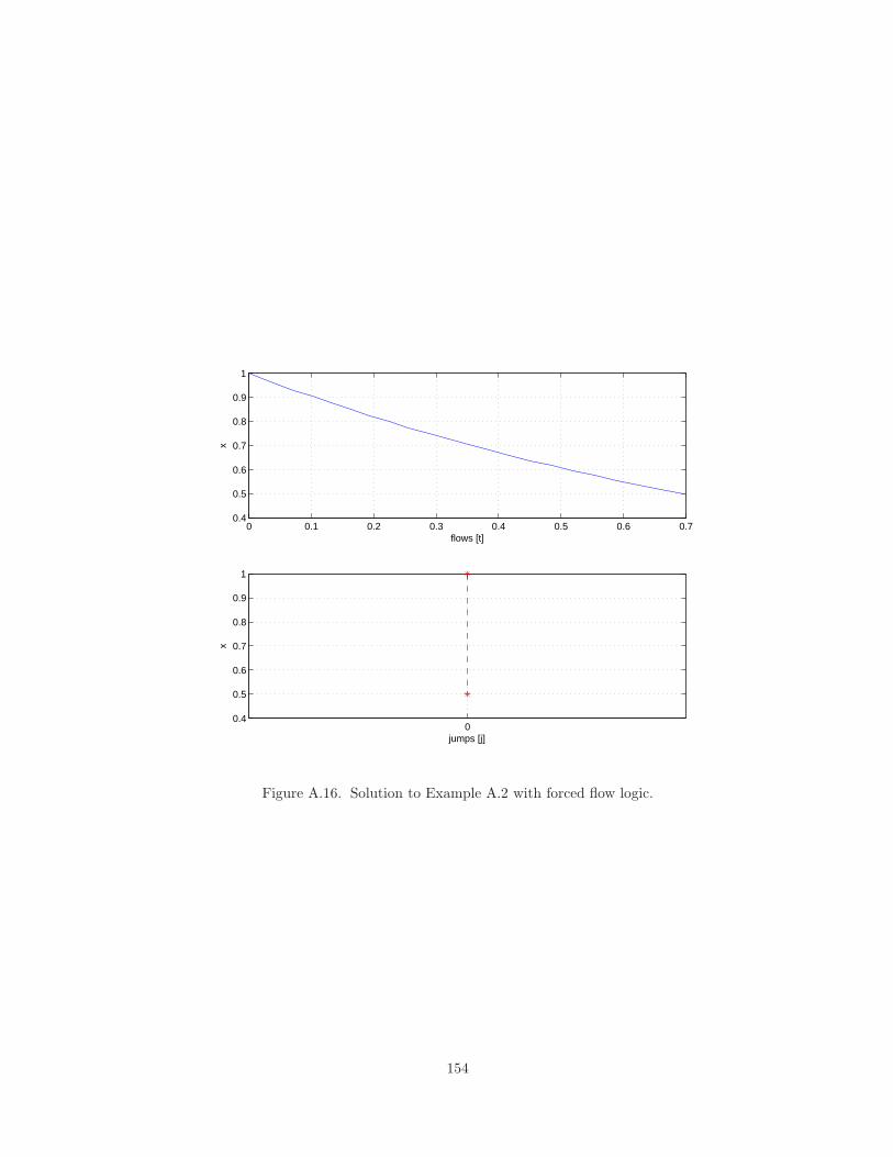
0 0.1 0.2 0.3 0.4 0.5 0.6 0.70.4

0.5

0.6

0.7

0.8

0.9

1

flows [t]

x

00.4

0.5

0.6

0.7

0.8

0.9

1

jumps [j]

x

Figure A.16. Solution to Example A.2 with forced flow logic.

154

Appendix B

Proofs

This appendix contains proofs that, for clarity of the exposition, were omitted throughout the thesis.

B.1 Proofs of results in Chapter 3

B.1.1 Proof of Theorem 3.11 and Corollary 3.15

The proof of these results is divided in two parts. In the next two sections, it is shown that Krasovskii solutionsare (control) Hermes solutions, and in the last section, it is shown that (control) Hermes solutions are Krasovskiisolutions.

Krasovskii solutions are Hermes

Theorem B.3 below is an extension of Theorem 5.5 in [42] to differential equations with a constraint x(t) ∈ C.Our proof is also different (and shorter) than that given in [42]. We will need the corollary of [42, Lemma 3.3]below.

Assumption B.1 (f and g assumptions) The set O ⊂ Rn is open. The sets C and D are subsets of O. The

function f : C → Rn is locally bounded on O. The set-valued mapping G : D →→ R

n is locally bounded withrespect to O on O.

Lemma B.2 (auxiliary lemma) Let f satisfy Assumption B.1 and let ψ : [0, T ] → O be an absolutely continuousfunction that satisfies, for almost all t ∈ [0, T ], ψ(t) ∈ f(ψ(t)). Then, for every ε > 0, there is a closed null-setZ and a Lipschitz function z : [0, T ] → O such that |ψ(t) − z(t)| ≤ ε for all t ∈ [0, T ] and which is piecewiselinear in the sense that z(t) = ψ(α) for all t in any component (α, β) of [0, T ] \Z, and for any such component,ψ(α) ∈ f(ψ(α)).

Above, by a component of (the open set) [0, T ] \ Z we understand any of the (at most countably many)mutually disjoint intervals (α, β) covering [0, T ] \ Z. In what follows, we will refer to the family of all suchintervals as I. Below, we will also use the term “piecewise constant” to mean that a function is constant oneach (α, β) ∈ I. Finally, we note that directly from the proof of the result above one can deduce that the sizeof the intervals (α, β) in I can be made arbitrarily small.

155

Theorem B.3 (continuous-time Krasovskii is Hermes) Let f satisfy Assumption B.1 and let ψ : [0, T ] → O bean absolutely continuous function that satisfies, for almost all t ∈ [0, T ], ψ(t) ∈ C, ψ(t) ∈ f(ψ(t)). Then, forany ε > 0 such that rgeψ + εB ⊂ O and any ϕ0 ∈ C such that |ϕ0 − ψ(0)| < ε, there exists a Lipschitz andpiecewise linear ϕ : [0, T ] → O with ϕ(0) = ϕ0 and a measurable e : [0, T ] → R

n such that supt∈[0,T ] |e(t)| ≤ ε,ϕ+ e is piecewise constant on [0, T ],

ϕ(t) + e(t) ∈ C for all t ∈ [0, T ], ϕ(t) = f(ϕ(t) + e(t)) for almost all t ∈ [0, T ],

and |ψ(t) − ϕ(t)| ≤ ε for all t ∈ [0, T ].

Proof. Fix ε > 0 so that rgeψ+εB ⊂ O, pick ϕ0 ∈ C so that |ϕ0−ψ(0)| < ε, and pick any ε′ ∈ (0, ε−|ϕ0−ψ(0)|).Let L > 0 be a bound on f on rgeψ + ε′B (so in particular, L is a Lipschitz constant for ψ). Use Lemma B.2

to obtain z : [0, T ] → O with |ψ(t) − z(t)| ≤ ε′/8 in a way that β − α ≤ ε′

8(1+L) for each component (α, β) of

[0, T ]\Z. Then, in particular, |ψ(t)−ψ(α)| ≤ ε′/8 for all t ∈ (α, β) and all intervals (α, β) in I. For each segment(α, β) ∈ I, by the definition of f and since ψ(α) ∈ f(ψ(α)), there exist points ψα

j ∈ C, j = 1, 2, . . . , n+ 1, so

that |ψαj − ψ(α)| ≤ ε′/8 and constants λα

j ≥ 0, j = 1, 2, . . . , n+ 1, so that∑n+1

j=1 λαj = 1 and

∣∣∣∣∣∣

n+1∑

j=1

λαj f(ψα

j )

− ψ(α)

∣∣∣∣∣∣≤ ε′

8(1 + T ).

Divide (α, β) into n + 1 subintervals (γαj−1, γ

αj ) with γα

0 = α, γαn+1 = β of lengths λα

j (β − α). Now definea piecewise linear function v : [0, T ] → R

n almost everywhere by v(t) = f(ψαj ) on (γα

j−1, γαj ). Note that

v ∈ L1[0, T ], and consequently, the function ϕ : [0, T ] → Rn defined by

ϕ(t) = ϕ0 +

∫ t

0

v(τ) dτ

is absolutely continuous. Furthermore, ϕ(t) = v(t) for almost all t ∈ [0, T ] (in fact, whenever t ∈ (γαj−1, γ

αj ), j =

1, 2, . . . , n+ 1). Also, define e : [0, T ] → Rn as follows: set

e(t) = ψαj − ϕ(t) if t ∈ (γα

j−1, γαj )

and note that this defines e for almost all t ∈ [0, T ], and that for those t’s, we have ϕ(t) = f(ϕ(t) + e(t)) aswell as ϕ(t) + e(t) ∈ C. For each t at which e(t) has not been defined yet, one can find ct ∈ C such that|ct − ψ(t)| < ε′/4 and then set e(t) = c − ϕ(t). Then ϕ(t) + e(t) ∈ C for all t ∈ [0, T ]. Also, ϕ(t) + e(t) isconstant on each (γα

j−1, γαj ), as so ϕ + e is piecewise constant on [0, T ]. We claim that ϕ and e have the other

desired properties.

For each initial point α of some interval (α, β) ∈ I

|ϕ(α) − z(α)| ≤ |ϕ(0) − z(0)| +∣∣∣∣∫ α

0

(ϕ(t) − z(t)) dt

∣∣∣∣

≤ |ϕ0 − z(0)|+∑

(α,β)∈I,β≤α

∣∣∣∣∣

∫ β

α

ϕ(t) dt− ψ(α)(β − α)

∣∣∣∣∣

≤ |ϕ0 − ψ(0)| + |ψ(0) − z(0)| +∑

(α,β)∈I,β≤α

ε′(β − α)

8(1 + T )

≤ |ϕ0 − ψ(0)| + ε′/8 +ε′

8(1 + T )

∑

(α,β)∈I,β≤α

(β − α)

= |ϕ0 − ψ(0)| + ε′/8 +ε′

8(1 + T )α

156

≤ |ϕ0 − ψ(0)| + ε′/4

where the sum above is over all intervals (α, β) ∈ I with β ≤ α (so that in particular,∑

(β − α) = α) and thelast inequality above relies on α < T . 1 Furthermore, for each interval (α, β) and any τ ∈ (α, β),

∣∣∣∣∫ τ

α

ϕ(t) dt− ψ(α)(τ − α)

∣∣∣∣ ≤ 2L(τ − α) ≤ 2L(β − α) ≤ ε′/4

since both ϕ and ψ are bounded by L. Consequently,

|ϕ(t) − z(t)| ≤ |ϕ0 − ψ(0)| + ε′/2

for all t ∈ [0, T ], and hence|ϕ(t) − ψ(t)| ≤ |ϕ0 − ψ(0)| + 5ε′/8 < ε

for all t ∈ [0, T ].

For the error bound, one obtains, for t in one of the intervals (γαj−1, γ

αj ),

|e(t)| ≤∣∣ψα

j − ψ(α)∣∣ + |ψ(α) − ψ(t)| + |ψ(t) − ϕ(t)|

≤ ε′/8 + ε′/8 + |ϕ0 − ψ(0)| + 5ε′/8= |ϕ0 − ψ(0)| + 7ε′/8 < ε.

For the remaining t’s,

|e(t)| ≤ |ct − ψ(t)| + |ψ(t) − ϕ(t)| ≤ ε′/4 + |ϕ0 − ψ(0)| + 5ε′/8 < ε

by the choice of ct and the previously established bound on |ψ(t) − ϕ(t)|. Thus |e(t)| ≤ ε for all t ∈ [0, T ].

Theorem B.4 (Krasovskii solution is close to a Hermes solution) Let Assumption B.1 hold and let ψ : domψ →O be a Krasovskii solution to the hybrid system H = (O, f, C, g,D). Pick any ε > 0 and any (T, J) ∈ domψ.

Let E = domψ ∩ ([0, T ]×0, 1, . . . , J) and express E as⋃J

j=0([tj , tj+1]×j). Then, there exist a measurablefunction e : dom e → R

n, dom e = E and a hybrid arc ϕ : domϕ → O, ϕ(0, 0) = ψ(0, 0), domϕ = E such thatsup(t,j)∈dom e |e(t, j)| ≤ ε and

(V1) for all j = 0, 1, . . . , J ,

ϕ(t, j) + e(t, j) ∈ C for all t ∈ [tj , tj+1), ϕ(t, j) = f(ϕ(t, j) + e(t, j))

for almost all t ∈ [tj , tj+1];

(V2) for all j = 0, 1, . . . , J − 1,

ϕ(tj+1, j) + e(tj+1, j) ∈ D, ϕ(tj+1, j + 1) ∈ g(ϕ(tj+1, j) + e(t, j));

1We used the fact that by the construction of v, for any (α, β) in I,

Z β

α

ϕ(t) dt =

n+1X

j=1

Z γαj

γαj−1

v(t) dt =

n+1X

j=1

λαj (β − α)f(ψα

j ) = (β − α)

n+1X

j=1

λαj f(ψα

j )

and thus˛

˛

˛

˛

Z β

α

ϕ(t) dt − ψ(α)(β − α)

˛

˛

˛

˛

≤ (β − α)

˛

˛

˛

˛

˛

˛

n+1X

j=1

λαj f(ψα

j ) − ψ(α)

˛

˛

˛

˛

˛

˛

≤ ε′(β − α)

8(1 + T ).

157

and |ϕ(t, j) − ψ(t, j)| ≤ ε for every (t, j) ∈ domϕ.

Proof. Fix ε > 0 small enough so that ψ(t, j) + εB ⊂ O for all (t, j) ∈ E. Note that for each j = 0, 1, . . . , J − 1there exists zj ∈ D and wj+1 ∈ g(zj) such that |zj − ψ(tj+1, j)| ≤ ε

8 and |wj+1 − ψ(tj+1, j + 1)| ≤ ε8 . Indeed,

for any x ∈ D and ǫ > 0, we have:

g(x) ⊂ g((x+ ǫB) ∩D) ∩O ⊂ (g((x+ ǫB) ∩D) + ǫB) ∩O,where the first inclusion above comes from the definition of g(x), and the second one from the definition ofthe closure of a set. Consequently, for each y ∈ g(x), there exists z ∈ (x + ǫB) ∩ D and w ∈ g(z) such thaty ∈ g(y) + ǫB.

On each segment [tj , tj+1] × j that is nontrivial, i.e., with tj+1 > tj , by Theorem B.3, there exists anabsolutely continuous function ϕj : [tj , tj+1] → O starting at ϕ0

j ∈ ψ(tj , j) + ε8B, where ϕ0

j = wj if j > 0,

ϕ0j = ψ(0, 0) if j = 0, and a measurable function ej : [tj , tj+1] → R

n with supt∈[tj ,tj+1] |ej(t)| ≤ ε4 satisfying

ϕj(t) + ej(t) ∈ C for all t ∈ [tj , tj+1], ϕj(t) = f(ϕj(t) + ej(t))

for almost all t ∈ [tj , tj+1], and such that

|ϕj(t) − ψ(t, j)| ≤ ε

4for all t ∈ [tj , tj+1] .

We now construct the measurement noise e. On each segment [tj , tj+1]×j ⊂ E that is trivial, i.e segmentswith tj+1 = tj , let e′j = zj −wj if J > j > 0, e′j = z0 − ψ(0, 0) if j = 0, and e′j = 0 if j = J . On each nontrivialsegment [tj , tj+1] × j, let e′j(t) = ej(t) for all (t, j) ∈ [tj , tj+1) × j, e′j(tj+1) = zj − ϕj(tj+1) if j < J ,e′j(tj+1) = 0 if j = J .

Then, ϕ and e are given by

ϕ(t, j) :=

ϕj(t) if (t, j) ∈ [tj , tj+1] × j nontrivialwj if (t, j) = [tj , tj+1] × j trivial

e(t, j) :=

e′j(t) if (t, j) ∈ [tj , tj+1] × j nontriviale′j if (t, j) = [tj , tj+1] × j trivial .

By construction, ϕ and e satisfy (V1) and (V2). It follows that |ϕ(t, j)−ψ(t, j)| ≤ ε for all (t, j) ∈ domϕ sinceon every trivial segment

|ϕ(t, j) − ψ(t, j)| = |wj − ψ(t, j)| ≤ ε

8

and on every nontrivial segment [tj , tj+1] × j

|ϕ(t, j) − ψ(t, j)| = |ϕj(t) − ψ(t, j)| ≤ ε

4∀t ∈ [tj , tj+1] .

Moreover, sup(t,j)∈dom e |e(t, j)| ≤ ε since on every trivial interval

|e(t, j)| = |zj − wj | ≤ |zj − ψ(t, j)| + |ψ(t, j) − wj | ≤ ε4 if J > j > 0

|e(t, j)| = |z0 − ψ0| ≤ ε8 if j = 0

|e(t, j)| = 0 if j = J,

and on every nontrivial segment [tj , tj+1] × j

|e(t, j)| = |e′j(t)| = |ej(t)| ≤ε

4∀t ∈ [tj , tj+1)

|e(t, j)| = |zj − ϕj(t)| ≤ |zj − ψ(t, j)| + |ψ(t, j) − ϕj(t)| ≤ε

2

for all (t, j) = (tj+1, j) if j < J , and |e(t, j)| = 0 if j = J .

158

Corollary B.5 (Krasovskii solutions are Hermes solutions) Under Assumption B.1, if a hybrid arc is a hybridKrasovskii solution to H then it is also a Hermes solution to H.

Proof. Let ψ : domψ → O be a Krasovskii solution to H. Pick (T, J) ∈ domψ (when domψ is compact, it isenough to consider (T, J) = supdomψ). Let ψ′ be the truncation of ψ to domψ′ = domψ∩([0, T ]×0, 1, . . . , J).By Theorem B.4, there exist ei : domψ′ → R

n and ϕi : domψ′ → O such that sup(t,j)∈dom ei|ei(t, j)| ≤ 1

i andwhich satisfy conditions (V1) and (V2) of Theorem B.4 (with e replaced by ei and ϕ replaced by ϕi) and also|ψ(t, j) − ϕi(t, j)| ≤ 1/i for every (t, j) ∈ domϕi. The last bound implies that ϕi converge graphically to ψ′.Since sup(t,j)∈dom ei

|ei(t, j)| ≤ 1i , ψ is a Hermes solution to H.

Krasovskii solutions are control Hermes solutions

Below, we consider f and g given as in Corollary 3.11 with the assumption therein which, for convenience,we rewrite below. The result to follow is a corollary of Theorem B.3.

Assumption B.6 (f and g assumptions (control)) The set O ⊂ Rn is open. The sets C and D are subsets of

O. The function f ′ : O × Rmc → R

n is locally Lipschitz continuous in the first argument, locally uniformly inthe second argument. The function g′ : O × R

md → O is continuous in the first argument, locally uniformly inthe second argument. The functions κc : C → R

mc , κd : D → Rmd are locally bounded on O.

Corollary B.7 (continuous-time Krasovskii is control Hermes) Let f satisfy Assumption B.6, and let ψ :[0, T ] → R

n be an absolutely continuous function that satisfies, for almost all t ∈ [0, T ], ψ(t) ∈ C, ψ(t) ∈ f(ψ(t)).Let ε > 0 be small enough so that rgeψ+2εB ⊂ O and let L be a Lipschitz constant for f(·, u) on rgeψ+2εB ⊂ Ofor any u ∈ κc(rgeψ+2εB). Then, for every ϕ0 such that |ϕ0−ψ(0)| < εe−LT , there exists a measurable functione : [0, T ] → R

n and an absolutely continuous function ϕ : [0, T ] → O, ϕ(0) = ϕ0, such that supt∈[0,T ] |e(t)| ≤ ε,

ϕ(t) + e(t) ∈ C, for all t ∈ [0, T ],

ϕ(t) = f ′(ϕ(t), κc(ϕ(t) + e(t))) for almost all t ∈ [0, T ],

and |ϕ(t) − ψ(t)| ≤ ε for all t ∈ [0, T ].

Proof. Let ε > 0 be as assumed, and let ε′ = εe−LT < ε. By Theorem B.3, there exists an absolutely continuousfunction z : [0, T ] → O with z(0) = ϕ0 and a measurable function e′ : [0, T ] → R

n such that

z(t) = f ′(z(t) + e′(t), κc(z(t) + e′(t))) for almost all t ∈ [0, T ],

and |z(t) − ψ(t)| ≤ ε′, |e′(t)| ≤ ε′, and z(t) + e′(t) ∈ C for all t ∈ [0, T ]. Note that |(z(t) + e′(t)) − ψ(t)| ≤ 2ε′.Furthermore, z + e′ is piecewise constant on [0, T ], so κc(z(t) + e′(t)) is measurable, and so the mapping(x, t) 7→ f ′(x, κc(z(t) + e′(t)) is a Caratheodory mapping: continuous in x for a fixed t and measurable in t fora fixed x. Consequently, there exists a solution ϕ : [0, T ] → O to

ϕ(t) = f ′(ϕ(t), κc(z(t) + e′(t))) a.e. and ϕ(0) = ϕ0

for which ϕ(0) = z(0),

|ϕ(t) − z(t)| ≤ L|ϕ(t) − z(t) − e′(t)| ≤ L|ϕ(t) − z(t)| + Lε′

and thus |ϕ(t) − z(t)| ≤ ε′(eLT − 1) for all t ∈ [0, T ]. Consequently, for all t ∈ [0, T ],

|ϕ(t) − ψ(t)| ≤ |ϕ(t) − z(t)| + |z(t) − ψ(t)| ≤ ε′eLT = ε .

159

Let e(t) := z(t)+e′(t)−ϕ(t), so that z(t)+e′(t) = ϕ(t)+e(t). Then, since z(t)+e′(t) ∈ C, we have ϕ(t)+e(t) ∈ Cfor all t ∈ [0, T ]. Furthermore, ϕ(t) = f(ϕ(t), κc(ϕ(t) + e(t))). Finally,

|e(t)| ≤ |ϕ(t) − z(t)| + |e′(t)| ≤ ε′(eLT − 1) + ε′ = ε′eLT = ε .

The next result combines Corollary B.7 above, and the ideas of Theorem B.4.

Corollary B.8 (Krasovskii solution is close to a control Hermes solution) Let Assumption B.6 hold, and letψ : domψ → O be a Krasovskii solution to H = (O, f, C, g,D) with f and g as given in Corollary 3.15. Pick any

ε > 0 and any (T, J) ∈ domψ. Let E = domψ ∩ ([0, T ]×0, 1, . . . , J) and express E as⋃J

j=0([tj , tj+1]× j).Then, there exist a measurable function e : dom e → R

n, dom e = E and a hybrid arc ϕ : domϕ → O,ϕ(0, 0) = ψ(0, 0), domϕ = E such that sup(t,j)∈dom e |e(t, j)| ≤ ε and

(V1’) for all j = 0, 1, . . . , J ,

ϕ(t, j) + e(t, j) ∈ C for all t ∈ [tj , tj+1), ϕ(t, j) = f ′(ϕ(t, j), κc(ϕ(t, j) + e(t, j)))

for almost all t ∈ [tj , tj+1];

(V2’) for all j = 0, 1, . . . , J − 1,

ϕ(tj+1, j) + e(tj+1, j) ∈ D, ϕ(tj+1, j + 1) = g′(ϕ(tj+1, j), κd(ϕ(t, j) + e(t, j)));

and |ϕ(t, j) − ψ(t, j)| ≤ ε for every (t, j) ∈ domϕ.

Proof. Let S := domψ ∩ ([0, T ] × 0, 1, . . . , J), fix ε > 0 so that ψ(t, j) + 2εB ⊂ O for all (t, j) ∈ S, and letL be a Lipschitz constant for f(·, u) on ψ(t, j) + 2εB | (t, j) ∈ S. Note that for any δ > 0, at each jump of ψon S, i.e. at each point (t, j) ∈ S such that there exists (t, j + 1) ∈ S, we can find zj ∈ D arbitrarily close toψ(t, j) that satisfies |g(zj , κd(zj)) − ψ(t, j + 1)| ≤ δ/2. This was already justified in the proof of Theorem B.4.Since g is continuous in the first variable, locally uniformly in the second variable varying over compact sets,we can pick zj so that |g(ψ(t, j), κd(zj)) − ψ(t, j + 1)| ≤ δ. Thus, by using δ = min ε

8 ,ε4e

−LT, for every jumpof ψ we obtain points zj ∈ D such that |zj −ψ(t, j)| ≤ ε

8 and |g(ψ(t, j), κd(zj))−ψ(t, j + 1)| ≤ min ε8 ,

ε4e

−LT.On each segment [tj , tj+1] × j := S ∩ (R≥0 × j) ⊂ S that is nontrivial, i.e segments with tj+1 > tj ,

by Corollary B.7, there exists an absolutely continuous function ϕj : [tj , tj+1] → O starting at ϕ0j ∈ ψ(tj , j) +

min ε8 ,

ε4e

−LTB, where ϕ0j = g(ψ(tj , j), κd(zj−1)) if j > 0, ϕ0

j = ψ0 if j = 0, and a measurable functionej : [tj , tj+1] → R

n with supt∈[tj ,tj+1] |ej(t)| ≤ ε4 satisfying for almost all t ∈ [tj , tj+1]

ϕj(t) + ej(t) ∈ C, ϕj(t) = f ′(ϕj(t) + ej(t), κc(ϕ(t) + e(t)))

and for all t ∈ [tj , tj+1]

|ϕj(t) − ψ(t, j)| ≤ ε

4. (B.1)

The rest of the proof is analogous to that of Theorem B.4.

With Corollary B.8 at hand, the result below can be shown exactly in the same fashion as Corollary B.5.

Corollary B.9 (Krasovskii solutions are control Hermes solutions) Under Assumption B.6, if a hybrid arc is ahybrid Krasovskii solution to H then it is also a control Hermes solution to H.

160

Hermes and control Hermes solutions are Krasovskii solutions

Let ρ : O → (0,∞) be an admissible radius of perturbation, that is, a continuous function such that for all

x ∈ O, x+ ρ(x)B ⊂ O. For each δ ∈ (0, 1), let Hδ denote the hybrid system defined by sets

Cδ

:= x ∈ O |x+ δρ(x)B ∩ C 6= ∅, Dδ

:= x ∈ O |x+ δρ(x)B ∩D 6= ∅

and mappings

fδ(x) := co f((x + δρ(x)B) ∩ C) + δρ(x)B,

gδ(x) := ξ + δρ(ξ)B | ξ ∈ g((x+ δρ(x)B) ∩D).Such “inflations” of the hybrid system H were discussed in detail in [39]. A key property of such perturbations of

H is that, thanks to properties of H given by the hybrid basic conditions and subject to minor local boundednessconditions, a sequence of solutions to Hδ with decreasing δ is a solution to H. We will use this below.

Proposition B.10 (control Hermes solution is close to a Krasovskii solution) Under Assumption B.6, if ahybrid arc is a control Hermes solution to H, then it is also a Krasovskii solution to H.

Proof. Let ϕ : domϕ→ O be a control Hermes solution to H = (O, f, C, g,D). Pick (T, J) ∈ domϕ and let ϕ′

be the truncation of ϕ to domϕ′ given by domϕ ∩ ([0, T ]× 0, 1, . . . , J). Let the sequences of ϕi’s, ei’s, andεi’s correspond to ϕ′. In particular, for all i and all (t, j) ∈ dom ei, |ei(t, j)| ≤ εi and limi→∞ εi = 0.

For each j ∈ 0, 1, . . . , J, ϕi(·, j) converge graphically to ϕ′(·, j); this comes directly from the definition ofgraphical convergence. Since, for each j, the graphs of ϕi(·, j) are connected and the graph of ϕ′(·, j) is compact(in fact a compact subset of R≥0 ×N×O), for each j the graphs of ϕi(·, j) are eventually bounded with respectto O. This can be shown in the same fashion as [79, Corollary 4.12]. Consequently, there exists a compact setK ⊂ O and an index i0 such that ϕi(t, j) ∈ K for all i > i0, all (t, j) ∈ domϕi, j ≤ J .

Let ρ be any admissible perturbation radius. Then let ik > i0 be such that |εik| ≤ k−1 minρ(x) |x ∈ K,

and let ψk be the truncation of ϕikto domψik

:= (t, j) ∈ domϕik| j ≤ J. Fix k. For all k and almost all t

such that (t, j) ∈ domψk we have ψk(t, j) + eik(t, j) ∈ C ⊂ C and since |eik

(t, j)| ≤ k−1ρ(ψk(t, j)), we have

(ψk(t, j) + k−1ρ(ψk(t, j))

)∩ C 6= ∅

and consequently ψk(t, j) ∈ C1/k

. Furthermore, since for any δ ∈ (0, 1) and any x,

f ′(x, κc((x + δρ(x)B) ∩ C)) ⊂ f((x+ δρ(x)B) ∩ C) ⊂ f((x + δρ(x)B) ∩C) ⊂ fδ(x),

we have, for all k and almost all t such that (t, j) ∈ domψk, ψk(t, j) ∈ f1/k

(ψk(t, j)). Similar arguments show

that for all (t, j) ∈ domψk such that (t, j+1) ∈ domψk we have ψk(t, j) ∈ D1/k

and ψk(t, j+1) ∈ g1/k(ψk(t, j)).

Consequently, ψk is a solution to H1/k, for k = 1, 2, . . . . Since the sequence of ϕi’s converges graphically to ϕ′,by the very definition of graphical convergence, so does the sequence of ψk’s. Now, since ψk∞k=1 is eventuallybounded, its graphical limit, that is ϕ′, is a solution to H; see [39, Theorem 5.1 and Theorem 5.4]. Thus, ϕ′ isa Krasovskii solution to H. Since (T, J) was an arbitrary point in domϕ, this is sufficient to guarantee that ϕis a Krasovskii solution to H.

In the proof above, the local boundedness and continuity properties from Assumption B.6 are only neededto guarantee that f and g meet Assumption B.1, so that [39, Theorem 5.1 and Theorem 5.4] can be invoked.Furthermore, the proof can be repeated with little change for the case of a set valued g, as considered for Hermessolutions. The results of [39] still apply, and thus we obtain:

161

Corollary B.11 (Hermes solutions are Krasovskii solutions) Under Assumption B.1, if a hybrid arc is a Hermessolution to H, then it is also a Krasovskii solution to H.

Proof. Let ψ : domψ → O be a Krasovskii solution to H. Pick (T, J) ∈ domψ (when domψ is compact, it isenough to consider (T, J) = supdomψ). Let ψ′ be the truncation of ψ to domψ′ = domψ∩([0, T ]×0, 1, . . . , J).By Theorem B.4, there exist ei : domψ′ → R

n and ϕi : domψ′ → O such that sup(t,j)∈dom ei|ei(t, j)| ≤ 1

i andwhich satisfy conditions (V1) and (V2) of Theorem B.4 (with e replaced by ei and ϕ replaced by ϕi) and also|ψ(t, j) − ϕi(t, j)| ≤ 1/i for every (t, j) ∈ domϕi. The last bound implies that ϕi converge graphically to ψ′.Since sup(t,j)∈dom ei

|ei(t, j)| ≤ 1i , ψ is a Hermes solution to H.


B.2.1 Proof of Theorem 4.3

Stability of A is guaranteed by Theorem 4.16. To show attractivity, pick δ > 0 as in the last paragraph of theproof of Theorem 4.16. Pick any z ∈ A+ δB and any x ∈ SH(z). Then ΩH(x) ⊂ N , where N is given by (B.3),and in particular, Ω(x) ⊂ U . Given any z′ ∈ Ω(x), let ξ ∈ SH(z′) be any solution to H verifying the forwardinvariance of Ω(x), i.e. rge ξ ⊂ Ω(x). By Lemma B.12, V is constant along ξ. Suppose that V (ξ(t, j)) = d > 0for all (t, j) ∈ dom ξ, so in particular Ω(x) ∩ A = ∅. If assumptions (a) and (b) hold, then by (a) and LemmaB.12, ξ is instantaneously Zeno since Ω(x) ⊂ N . Hence, by (b), it converges to A. But this contradicts V beingconstant along ξ. If assumptions (a’) and (b’) hold, then by (a’) and Lemma B.12, ξ has no jumps, i.e. it is acomplete continuous solution. Hence, by (b’), it converges to A. This again contradicts V being constant alongξ. Thus, V (ξ(t, j)) = 0 for all (t, j) ∈ dom ξ and consequently, Ω(x) ⊂ A. This implies that x converges to A.


The bound (4.4) holds with uc, ud replaced by uC , uD, for any trajectory x with rgex ⊂ U . Consequently,by Theorem 4.17, any precompact trajectory x with rgex ⊂ U approaches the largest weakly invariant set in(4.10) for some r ∈ V (U) (with G = g), and here, the reachable set G(u−1

D (0)) is just G(u−1D (0)). Since uC

is upper semicontinuous and nonpositive on U , the set u−1C (0) is closed, and the closure can be omitted. The

same reasoning applies when assumptions involve vC or wC , however since these functions need not be uppersemicontinuous, the closures are necessary.

B.2.3 Proof of Corollary 4.15

If x is Zeno, then the weak invariance of Ω(x) can be verified by instantaneous Zeno trajectories. More specif-ically, given z ∈ Ω(x) with x(ti, ji) → z for some increasing and unbounded sequence of (ti, ji)’s, the sequenceof trajectories xi(t, j) := x(t + t(ji), j + ji − 1) has a graphically convergent subsequence, the limit ξ of whichhas the domain equal to 0 × N (see also the proof of Lemma 4.13) and is such that ξ(0, 1) = z. Using thislimit in the proof of Lemma B.13 shows that z ∈ u−1

d (0) ∩G(u−1d (0)).

Regarding (b), note that we can truncate x (and we won’t relabel it) so that, for some γ > 0, tj+1 − tj ≥ γfor all j ≥ 0 such that (tj , j), (tj+1, j) ∈ domx. Pick z ∈ Ω(x) and an increasing and unbounded sequence(ti, ji) with the property that x(ti, ji) → z. Suppose that the sequence given by xi(t, j) := x(t + ti, j + ji)graphically converges, say to a trajectory x ∈ SH, and x(0, 0) = z (consult the proof of Lemma 4.13). If

[0, γ/3]×0 ⊂ dom x, then using x in the proof of Lemma B.13 shows that z ∈ u−1c (0). In the opposite case, a

graphically convergent subsequence can be extracted from the sequence given by x′i(t, j) := x(t+ ti−γ/3, j+ ji)

162

so that its limit x′ is such that [0, γ/3] × 0 ⊂ dom x′. Furthermore x′(γ/3, 0) = z and rge x′ ⊂ Ω(x) (sox′ verifies the weak backward invariance of Ω(x) at z), and using x′ in the proof of Lemma B.13 shows that

z ∈ u−1c (0).


Assume (⋆) and let ǫ > 0 be small enough so that A + 2ǫB ⊂ U . We claim that there exists cǫ such that

V (z) ≤ cǫ, z ∈ (A + 2ǫB) ∩ (C ∪D)⇒ z ∈ (A + ǫB) ∩ (C ∪D), G(z) ⊂ (A + ǫB) ∩ (C ∪D).

(B.2)

Certainly, as V is positive definite on C ∪ D with respect to A, there exists r′ǫ > 0 so that for z ∈(A + 2ǫB) ∩ (C ∪D), V (z) ≤ r′ǫ implies z ∈ (A + ǫB) ∩ (C ∪D). Now note that as uD(z) ≤ 0 for all z ∈ A andV is positive definite on C ∪ D with respect to A, G(A ∩ (C ∪ D)) ⊂ A ∩ (C ∪ D). By outer semicontinuityand local boundedness, the mapping G is “upper semicontinuous”, in particular there exists γ > 0 so thatG(A+γB) ⊂ A+ ǫB. Using positive definiteness of V again, one can find r′′ǫ > 0 so that z ∈ (A+2ǫB)∩(C ∪D)and V (z) ≤ r′′ǫ imply z ∈ (A+γB)∩(C∪D). To make the implication (B.2) true, one now takes rǫ = minr′ǫ, r′′ǫ .

Based on (B.2), we claim that the set

N = z ∈ (A + ǫB) ∩ (C ∪D) | V (z) ≤ rǫ (B.3)

is (strongly) forward invariant for H, that is for any x ∈ SH(z) with z ∈ N , rgex ⊂ N . Indeed, pick anyz ∈ N and let x ∈ SH(z). If (0, 1) ∈ domx, then x(0, 1) ∈ G(z) ⊂ (A + ǫB) ∩ (C ∪D). If [0, T ]× 0 ⊂ domxand for some t′ ∈ (0, T ], x(t′, 0) 6∈ N , then by continuity of t 7→ x(t, 0), for some t′′ ∈ (0, t′], x(t′′, 0) 6∈ Nbut x(t′′, 0) ∈ (A + ǫB) ∩ (C ∪ D) and V (x(t′′, 0)) ≤ rǫ (the latter is true as V is nonincreasing along x). Byequation (B.2), x(t′′, 0) ∈ N . This is a contradiction. Thus x([0, T ], 0) ⊂ N . The facts just shown are enoughto conclude that N is forward invariant.

Finally, by continuity of V , given any small enough ǫ > 0 and rǫ > 0 so that (B.2) holds, we can findδ ∈ (0, ǫ) so that z ∈ (A+ δB) ∩ (C ∪D) implies V (z) ≤ rǫ. Relying on forward invariance of N , each maximalx ∈ SH(z) with z ∈ A + δB is so that rgex ⊂ A + ǫB. Thus, A is stable.

Now assume (⋆) and (⋆⋆). To show attractivity, note that given ǫ > 0 with A + 2ǫB ⊂ U , we can findrǫ ∈ (0, r), r as in condition (⋆⋆) so that N in (B.3) is forward invariant (i.e. one can pick rǫ in the proof ofstability of A arbitrarily small). In particular, if δ is associated with ǫ as in the paragraph above, any x ∈ SH(z)with z ∈ A + δB is precompact. As such, by Theorem 4.14, it converges to the largest weakly invariant subsetof the set given by (4.6). It must be the case that r′ ≤ rǫ as V is nonincreasing along x, and then r′ < r∗.As Ω(x) is nonempty, x converges to the largest weakly invariant subset of (4.6) with r = 0 which, by positivedefiniteness of V , is a subset of A. Hence, A is attractive.


The next two lemmas allow us to establish the V invariance principle for hybrid trajectories.

Lemma B.12 (V constant on Ω(x)) Suppose a function V : O → R is nonincreasing along a hybrid trajectoryx. If V is lower semicontinuous, then for some r ∈ R, V (Ω(x)) ⊂ (−∞, r]. If V is continuous, then for somer ∈ R, V (Ω(x)) = r.

Proof. If Ω(x) = ∅, there is nothing to prove. Otherwise, pick any z ∈ Ω(x). By the definition of Ω(x),there exists (ti, ji)∞i=1, an increasing and unbounded sequence in domx, satisfying x(ti, ji) → z. Let r =

163

lim infi→∞ V (x(ti, ji)). Pick any z ∈ Ω(x), and an increasing and unbounded sequence (tk, jk)∞k=1 in domxwith x(tk, jk) → z. There exists a subsequence (tki

, jki)∞i=1 of (tk, jk)∞k=1 such that for i = 1, 2, . . . , (ti, ji)

(tki, jki

), and as V is nonincreasing along x, V (x(ti, ji)) ≥ V (x(tki, jki

)). If V is lower semicontinuous, takinglimits as i → ∞ yields r ≥ lim infi→∞ V (x(tki

, jki)) ≥ V (z). If V is continuous, then let r = lim V (x(ti, ji)) =

V (z), and considering a subsequence (tik, jik

)∞k=1 of (ti, ji)∞i=1 so that (tk, jk) (tik, jik

) and V (x(tk, jk)) ≥V (x(tik

, jik)) yields, in the limit, that V (z) ≥ r. Thus, if V is continuous, V (z) = r.

Lemma B.13 (invariant sets with constant V ) Let V : O → R, uc, ud : O → [−∞,+∞] be any functions,the set U ⊂ O be such that uc(z) ≤ 0, ud(z) ≤ 0 for all z ∈ U and such that for any trajectory ξ ∈ SH withrge ξ ⊂ U , (4.4) holds for any (t, j), (t′, j′) ∈ dom ξ such that (t, j) (t′, j′). Let M ⊂ U be a set such that

V (M) = r for some r ∈ R. If M is weakly forward invariant, then M ⊂ u−1c (0) ∪ u−1

d (0). If M is weakly

backward invariant, then M ⊂ u−1c (0) ∪G(u−1

d (0)). If M is weakly invariant, then

M ⊂ u−1c (0) ∪

(u−1

d (0) ∩G(u−1d (0))

).

Proof. For any trajectory x ∈ SH such that x(t, j) ∈ M for (t, j) ∈ domx with (t, j) (t, j) (t, j) for some

(t, j) and (t, j) in domx, the fact that V is constant along trajectories in M gives

∫ t

t

uc(x(s, j(s))) ds +

j∑

i=j+1

ud(x(t(i), i− 1)) = 0.

Pick any z ∈ M. If M is weakly forward invariant, then there exists a nontrivial x ∈ SH(z) with rgex ⊂ M.If (0, 1) ∈ domx, applying the above equation to (t, j) = (0, 0), (t, j) = (0, 1) yields ud(x(0, 0)) = 0, which

shows that z ∈ u−1d (0). If (T, 0) ∈ domx for some T > 0, then applying the equation to (0, 0), (T, 0) yields∫ T

0uc(x(s, 0)) ds = 0. As uc is nonpositive, it must be the case that uc(x(s, 0)) = 0 for almost all s ∈ [0, T ].

Hence, z ∈ u−1c (0). If M is weakly backward invariant, then there exists x ∈ SH(z∗), z∗ ∈ M, such that

x(t∗, j∗) = z, t∗ + j∗ > 1, and x(t, j) ∈ M for all (t, j) (t∗, j∗). If (t∗, j∗ − 1) ∈ domx, then the inequalityabove with (t, j) = (t∗, j∗−1), (t, j) = (t∗, j∗) shows that ud(x(t

∗, j∗−1)) = 0 and so z = x(t∗, j∗) ∈ G(u−1d (0)).

If (t∗−T, j∗) ∈ domx for some T > 0, then an argument similar to the one for forward invariance can be given.

For any precompact trajectory x, from Lemma 4.13 we know that x approaches its ω-limit, which is weaklyinvariant. This ω-limit is the same as the ω-limit of the truncation of x to (t, j)’s with (T, J) (t, j) ∈ domx.By (4.4), the function V is nonincreasing along the truncation. Thus V is constant on Ω(x) by Lemma B.12.Now note that Ω(x) is a subset of U intersected with rge ξ | ξ ∈ SH, rge ξ ⊂ U. In turn, this intersectionmeets the conditions placed on the set U in Lemma B.13. Thus, invoking Lemma B.13, with M also replacedby Ω(x), finishes the proof.


(1 ⇒ 2) Let M be the largest weakly invariant set in K. Suppose that there exists z ∈ M \ A. Let ǫ = |z|A.By stability of A relative to K, there exists δ > 0 such that every hybrid trajectory ξ ∈ SH with rge ξ ⊂ Kand ξ(0, 0) ∈ A + δB satisfies rge ξ ⊂ A + ǫ

2B. By weak backward invariance of M, there exists a trajectoryx1 ∈ SH such that for some (t1, j1) ∈ domx1, t1 + j1 ≥ 1, x1(t1, j1) = z and x1(t, j) ∈ M for all (t, j) (t1, j1),(t, j) ∈ domx1 (in particular x1(0, 0) ∈ M). Note that by stability, since x1(t1, j1) 6∈ A + ǫ

2B, we havex1(t, j) ∈ M\ (A+ δB) for all (t, j) ∈ domx1, (t, j) (t1, j1). In this way, we can construct a sequence xi ∈ SH

164

such that for every i > 0, there exists (ti, ji) ∈ domxi, ti + ji ≥ i with xi(ti, ji) = z and xi(t, j) ∈ M\ (A+ δB)for all (t, j) (ti, ji), (t, j) ∈ domxi. As K is compact, the sequence xi∞i=1 is locally eventually bounded.By the hybrid basic conditions, it has a subsequence (that we won’t relabel) converging to some x ∈ SH,with xi(0, 0) → x(0, 0) ∈ M. Since domxi are “increasing”, x is complete; see [39, Lemma 3.5]. Finally,rgex ⊂ M \ (A + δB), and also rgex ⊂ K. The second inclusion, by detectability of A relative to K, relativestability of A, and Lemma 4.29, implies that x converges to A. This is a contradiction with the first inclusion.

(2 ⇒ 1) Any trajectory x ∈ SH with rgex ⊂ K is precompact, by compactness of K, and as such, itconverges to its ω-limit. Since the ω-limit is invariant and a subset of K, it must be a subset of A. Hence, xconverges to A.


Some of the following results use theorems from [39], which for completeness are reproduced below.

Theorem B.14 (KLL-bound [39, Theorem 6.5]) Suppose that the basin of attraction BA of a compact setA ⊂ O is open relative to C ∪ D. Let U ⊂ O be any open set such that BA = (C ∪D) ∩ U . For each properindicator ω : U → R≥0 of A with respect to U there exists β ∈ KLL such that, for all solutions x starting inBA,

ω(x(t, j)) ≤ β(ω(x(0, 0)), t, j) ∀(t, j) ∈ domx . (B.4)

Theorem B.15 (KLL-bound under perturbations [39, Theorem 6.6]) Suppose that the basin of attraction BA

of a compact set A ⊂ O is open relative to C ∪ D, U ⊂ O is any open set such that BA = (C ∪D) ∩ U , andω : U → R≥0 is a proper indicator of A with respect to U , and β ∈ KLL is such that, for all solutions startingin BA, (B.4) holds. Assume that the family of perturbed hybrid systems Hδ, δ ∈ (0, 1), has the convergenceproperty (CP) in [39, Section V]. Then, for each compact set K ⊂ BA and each ε > 0 there exists δ∗ > 0 suchthat for each δ ∈ (0, δ∗], the solutions xδ of Hδ from K satisfy, for all (t, j) ∈ domxδ,

ω(xδ(t, j)) ≤ β(ω(xδ(0, 0)), t, j) + ε ∀(t, j) ∈ domx .


To show Theorem 5.12, we first exploit the asymptotic stability of A with respect to Hcl. Using the propertiesof the data defining the closed-loop system Hcl to invoke the converse Lyapunov theorems for hybrid systemsin [23], there exists a smooth function V : R

np × Rnc → R≥0 and class-K∞ functions α1, α2 satisfying

i) ∀(x, xc) ∈ Rnp × R

nc : α1(|(x, xc)|A) ≤ V (x, xc) ≤ α2(|(x, xc)|A), (B.5)

ii) ∀(x, xc) ∈ Cc : 〈∇V (x, xc), [fp(x, κ(x, xc))T , fc(x, xc)

T ]T 〉 ≤ −V (x, xc), (B.6)

iii) ∀(x, xc) ∈ Dc : maxξ∈Gc(x,xc)

V (x, ξ) ≤ e−1V (x, xc), (B.7)

where we have used the properties of the data of Hcl.

By using continuity of V and (B.6), for each 0 < δs ≤ ∆s <∞ there exists δ > 0 and γ0 ∈ (0, 1) such thatfor all (x, xc) ∈ (Cc + δB) ∩ ΩA(δs,∆s)

〈∇V (x, xc), [f(x, κc(x, xc))T , fc(x, xc)

T ]T 〉≤ −γ0V (x, xc).

165

By local boundedness of (x, xc) 7→ fp(x, κc(x, xc)) and fc, there exists M > 0 such that for all (x, xc) ∈(Cc + δB) ∩ ΩA(0,∆s)

|[fp(x, κc(x, xc))T , fc(x, xc)

T ]T | ≤M .

Let 0 < δ < δ and pick Ts and Tc so that maxTs, Tc < δ/M . Note that with this construction, when flowsare enabled, points in Cc are not reachable from R

n × Rnc \ (Cc + δB) and points in R

n × Rnc \ (Cc + δB) are

not reachable from Cc.

We extend the hybrid system HS/Hcl with two auxiliary states: a continuous state denoted by zh and a

discrete state denoted by q. The continuous state zh is so that its update law is equal to the one for zc, whileits continuous dynamics are so that the flows of zh are governed by fc, i.e.

˙zh = fc(x, zh) (B.8)

when τs ∈ [0, Ts] and τc ∈ [0, Tc].

The discrete state q assumes values in the set 0, 1. We design the update law for q so that it is equal to 1when the new values of (zm, zh) are in the proximity of the flow set Cc, and zero when they are away from the

flow set Cc. During flows, q remains constant. We denote the extended hybrid system by HS/He

cl .

Let λ1, λ2, λ3 ∈ R be constants satisfying λ1, λ2 > 0, λ3 < 0, and let W (x, zh, τs, τc, q) be given by

W (x, zh, τs, τc, q) := exp(λ1τs) exp(λ2qτc) exp(λ3(1 − q)τc)V (x, zh) . (B.9)

The function W is constructed by combining the Lyapunov function V for the nominal closed-loop system Hcl

and exponential terms that depend on the timers τs, τc and the logic state q. The purpose of the exponentialterms in W is to balance the increase of

〈∇V (x, zh), [f(x, κc(zs, zc))T , fc(x, zh)T ]T 〉

along flows and of V (x, z+h ) − V (x, zh) at jumps. Clearly, during flows, the terms exp(λ1τs) and exp(λ2qτc)

for q = 1 decrease. However, at jumps, the terms exp(λ2qτc) and exp(λ3(1 − q)τc) may increase or decreasedepending on the value of q+. Therefore, the constants λ1, λ2, and λ3 have to be designed carefully to obtaindecrease both at flows . Let

e1 := zh − gfc(zm, zc), e2 := zm − x, e3 := zc − zh, e4 := zs − x .

The partial closed-loop system state [x, zh, τs, τc, q]T has continuous dynamics given by

f(x, zh, τs, τc, q) := [f(x, κc(zs, zc))T , fc(x, zh)T , 1, 1, 0]T .

The following lemma states a decrease property of W along flows for a proper choice of its constants.

Lemma B.16 (decrease along flows) Let Assumptions 5.1, 5.2, and 5.3 hold. Then, for each positive numberδs and ∆s satisfying 0 < δs ≤ ∆s < ∞ there exist ε > 0 and constants λ1 > 0, λ2 > 0, and λ3 < 0 of W suchthat

〈∇W (x, zh, τs, τc, q), f(x, zh, τs, τc, q)〉 ≤ −εW (x, zh, τs, τc, q)

for points

(F1) (x, zh, τs, τc, q, |[eT3 , e

T4 ]T |) ∈ ((Cc + δB) ∩ ΩA(δs,∆s)) × [0, Ts] × [0, Tc] × 1 × δ34B;

166

(F2) (x, zh, τs, τc, q, |[eT3 , e

T4 ]T |) ∈ ΩA(δs,∆s) × [0, Ts] × [0, Tc] × 0 × δ34B;

for some δ34 > 0.

Proof. When τs ≤ Ts and τc ≤ Tc, with the closed-loop dynamics we obtain

〈∇W (x, zh, τs, τc, q), f(x, zh, τs, τc, q)〉 ≤ (λ1 + λ2q + λ3(1 − q)) exp(λ1τs) exp(λ2qτc) exp(λ3(1 − q)τc)V (x, zh)+

exp(λ1τs) exp(λ2qτc) exp(λ3(1 − q)τc)〈∇V (x, zh), [f(x, κc(zs, zc))T , fc(x, zh)T ]T 〉.

By operating with the last term, we can rewrite the inequality as follows:

〈∇W (x, zh, τs, τc, q), f(x, zh, τs, τc, q)〉 ≤ (λ1 + λ2q + λ3(1 − q)) exp(λ1τs) exp(λ2qτc) exp(λ3(1 − q)τc)V (x, zh)+

exp(λ1τs) exp(λ2qτc) exp(λ3(1 − q)τc)〈∇V (x, zh), [f(x, κc(x, zh))T , fc(x, zh)T ]T 〉 exp(λ1τs) exp(λ2qτc)

exp(λ3(1 − q)τc)ρ(x, zh, τs, τc, q, e3, e4)

where

ρ(x, zh, τs, τc, q, e3, e4) := |∇V (x, zh)||f(x, κc(x+ e4, zh + e3)) − f(x, κc(x, zh))| .

The function ρ is continuous and for every (x, zh, τs, τc, q) ∈ Rn × R

m × R≥02 × 0, 1 then we have

ρ(x, zh, τs, τc, q, 0, 0) = 0 .

For all (x, zh) ∈ (Cc + δB) ∩ ΩA(δs,∆s) and q = 1, with the property of V in (B.8) there exists λ1 > 0,λ2 > 0, and ε > 0 satisfying −γ0 + λ1 + λ2 < −2ε that yields

〈∇W (x, zh, τs, τc, q), f(x, zh, τs, τc, q)〉 ≤ exp(λ1τs) exp(λ2τc)(−2εV (x, zh) + ρ(x, zh, τs, τc, q, e3, e4)).

Since ρ is continuous and vanishes with (e3, e4), there exists small enough δ34 > 0 so that (x, zh, τs, τc, |[eT3 , e

T4 ]T |)

in

ΩA(δs,∆s) × [0, Ts] × [0, Tc] × δ34B

implies

ρ(x, zh, τs, τc, q, e3, e4) < εV (x, zh) .

Then


for all (x, zh, τs, τc, q, |[eT3 , e

T4 ]T |) ∈ ((Cc + δB) ∩ ΩA(δs,∆s)) × [0, Ts] × [0, Tc] × 1 × δ34B.

When q = 0 we have that

〈∇W (x, zh, τs, τc, q), f(x, zh, τs, τc, q)〉 ≤ (λ1 + λ3) exp(λ1τs) exp(λ3τc)V (x, zh)+

exp(λ1τs) exp(λ3τc)〈∇V (x, zh), [f(x, κc(x, zh))T , fc(x, zh)T ]T 〉 + exp(λ1τs) exp(λ3τc)ρ(x, zh, τs, τc, q, e3, e4) .

Let MV be such that

max(x,ezh)∈ΩA(δs,∆s)

|∇V (x, zh)| |[f(x, κc(x, zh))T , fc(x, zh)T ]T | < MV .

Let µ ≥ MV

α1(δs) . It follows by (B.5) that

|〈∇V (x, zh), [f(x, κc(x, zh))T , fc(x, zh)T ]T 〉| ≤ µV (x, zh)

167

for all (x, zh) ∈ ΩA(δs,∆s). Then choose λ3 < 0 so that λ1 +λ3 +µ < − 32ε. Proceeding as for q = 1, we obtain


for all (x, zh, τs, τc, q, |[eT3 , e

T4 ]T |) ∈ ΩA(δs,∆s) × [0, Ts] × [0, Tc] × 0 × δ34B.

Lemma B.17 (decrease along jumps) Let Assumptions 5.1, 5.2, and 5.3 hold. Then for each positive numberδs and ∆s satisfying 0 < δs ≤ ∆s < ∞ and each constants λ1 > 0, λ2 > 0, and λ3 < 0 of W and Tc, Ts > 0satisfying Tcλ3 ∈ (−1, 0) there exists ρ ∈ (0, 1) such that

W (x+, z+h , τ

+s , τ

+c , q

+) ≤ ρW (x, zh, τs, τc, q)

for points

(J1) (x, zh, τs, τc, q) ∈ ΩA(δs,∆s) × [Ts,+∞) × [0, Tc] × 0, 1;

(J2) (zm, zc) ∈ Cc, (x, zh, τs, τc, q, |e1|) ∈ ΩA(δs,∆s) × [0, Ts] × [Tc,+∞) × 1 × δ1B;

(J3) (zm, zc) ∈ Dc, (x, zh, τs, τc, q, |[eT2 , e

T3 ]T |) ∈ ΩA(δs,∆s) × [0, Ts] × [Tc,+∞) × 0, 1 × δ23B;

for some δ1, δ23 > 0.

Proof. When τs ≥ Ts, for every λ1 > 0, Ts > 0 there exists ρ1 ∈ (0, 1) that satisfies ρ1 > exp(−λ1Ts) andyields

W (x+, z+h , τ

+s , τ

+c , q

+) = exp(λ2qτc) exp(λ3(1 − q)τc)V (x, zh) ≤ ρ1W (x, zh, τs, τc, q)

for all (x, zh, τs, τc, q) ∈ ΩA(δs,∆s) × [Ts,+∞) × [0, Tc] × 0, 1 since λ2 > 0.

When τc ≥ Tc, (zm, zc) ∈ Cc \Dc, and q = 1, the update law yields

W (x+, z+h , τ

+s , τ

+c , q

+) = exp(λ1τs)V (x, gfc(zm, zc)) . (B.10)

Since V is smooth on Rn, for every δ′ > 0 there exists L > 0 such that |η1 − η2| ≤ δ′, η1, η2 ∈ ΩA(0,∆s) ∩ R

n

implies

|V (η1) − V (η2)| ≤ Lδ′ . (B.11)

Let δ1 > 0 to be fixed later. Using (B.11) with δ′ = δ1 in (B.10), for every (x, zh, τs, τc, q, |e1|) ∈ ΩA(δs,∆s) ×[0, Ts] × [Tc,+∞) × 1 × δ1B we obtain

W (x+, z+h , τ

+s , τ

+c , q

+) ≤ exp(λ1τs)(V (x, zh) + Lδ1) .

Since V (x, zh) ≥ α1(δs) for every (x, zh) ∈ ΩA(δs,∆s), for every λ2 > 0, Tc > 0 there exists ρ2 ∈ (0, 1) satisfyingρ2 > exp(−λ2Tc) and by fixing δ1 to satisfy δ1 <

1Lα1(δs)(ρ2 exp(λ2Tc) − 1) we obtain

W (x+, z+h , τ

+s , τ

+c , q

+) ≤ ρ2W (x, zh, τs, τc, q) (B.12)

for all (zm, zc) ∈ Cc \Dc, (x, zh, τs, τc, q, |e1|) ∈ ΩA(δs,∆s) × [0, Ts] × [Tc,+∞) × 1 × δ1B.

When τc ≥ Tc and (zm, zc) ∈ Dc \Dc, the update law yields

W (x+, z+h , τ

+s , τ

+c , q

+) = exp(λ1τs)V (x, gc(zm, zc)) (B.13)

168

Let δ23 > 0 to be fixed later. Using δ′ = δ23 in (B.11) and the property of V at jumps in (B.7), for every(x, zh, τs, τc, q, |e2|) ∈ ΩA(δs,∆s) × [0, Ts] × [Tc,+∞) × 1 × δ23B we obtain

W (x+, z+h , τ

+s , τ

+c , q

+) ≤ exp(λ1τs)(e−1V (zm, zc) + Lδ23)

Using the smoothness of V again, for every

(x, zh, τs, τc, q, |[eT2 , e

T3 ]T |) ∈ ΩA(δs,∆s) × [0, Ts] × [Tc,+∞) × 1 × δ23B

it follows that

W (x+, z+h , τ

+s , τ

+c , q

+) ≤ exp(λ1τs)(e−1V (x, zh) + Lδ23(1 + e−1)) .

Since V (x, zh) ≥ α1(δs) for every (x, zh) ∈ ΩA(δs,∆s), for every Tcλ3 ∈ (−1, 0) there exists ρ3 ∈ (0, 1) satisfyingρ3 > exp(−λ3Tc − 1) and by fixing δ23 to satisfy δ23 <

1L(1+e)α1(δs)(ρ3 exp(λ3Tc + 1) − 1) we obtain

W (x+, z+h , τ

+s , τ

+c , q

+) ≤ ρ3W (x, zh, τs, τc, q) . (B.14)

for all (zm, zc) ∈ Dc \Cc, (x, zh, τs, τc, q, |[eT2 , e

T3 ]T |) ∈ ΩA(δs,∆s)× [0, Ts]× [Tc,+∞)×0, 1× δ23B. Following

the last two cases of the proof it is easy to show a similar result for points (zm, zc) ∈ Dc ∩ Cc.

In order to keep overall boundedness, the timer constants Ts, Tc > 0 need to be designed so that duringflows and jumps the error states ei, i = 1, 2, 3, 4, remain bounded. We establish this as follows.

Lemma B.18 (errors boundedness) Let Assumptions 5.1, 5.2, and 5.3 hold. For each positive numbers δs and

∆s satisfying 0 ≤ δs ≤ ∆s <∞, given δ′ > 0 there exists Tc, Ts > 0 so that for every solution ξe to HS/He

cl with(x0, z0

h) ∈ ΩA(δs,∆s) there exists (T ∗, J∗) ∈ dom ξe so that

|e2(t, j)| ≤ δ′, |e3(t, j)| ≤ δ′, |e4(t, j)| ≤ δ′, (B.15)

for every (t, j) (T ∗, J∗), (t, j) ∈ dom ξe.

Proof. Recall that the dynamics of HS/He

cl are such that during flows

e2 = −f(x, κc(zs, zc)), e3 = −fc(x, zh), e4 = −f(x, κc(zs, zc)); (B.16)

at jumps due to τs ≥ Ts

e+2 = e2, e+3 = e3, e+4 = 0; (B.17)

and at jumps due to τc ≥ Tc

e+2 = e4, e+3 = 0, e+4 = e4 . (B.18)

Let M0 = |[e2(0)T , e3(0)T , e4(0)T ]T | + δ′ + 1. Let M1 and M2 be two positive numbers satisfying


|fc(x, zh)| ≤M1, (B.19)


|f(x, κc(x+M0B, zh +M0B))| ≤M2 (B.20)

Since the jumps of HS/He

cl are triggered by the timers τs and τc, for every solution ξe there exists (T ∗, J∗) ∈ dom ξesuch that the jump mappings (B.17) and (B.18) have already been executed at least once, independently of the

169

point with (x0, z0h) ∈ ΩA(δs,∆s) from where ξe started from. Then, for all (t, j) (T ∗, J∗), (t, j) ∈ dom ξe,

using (B.19)-(B.16), |e3| cannot grow more than M1Tc, M1Tc < 1, and |e4| cannot grow more than M2Ts,M2Ts < 1, during flows. From (B.17) and (B.18), |e3| and |e4| do not increase during jumps. Then choose Tc

so that M1Tc ≤ min1, δ′

2 and Ts so that M2Ts ≤ min1, δ′

2 to show

|e3(t, j)| ≤δ′

2, |e4(t, j)| ≤

δ′

2, (B.21)

for every (t, j) (T ∗, J∗), (t, j) ∈ dom ξe. Since e2 is reset to e4 at jumps triggered by τc ≥ Tc, using (B.21) the

error |e2| cannot increase more than δ′ +M2Tc, M2Tc < 1. Then choose Tc so that M2Tc < min1, δ′

2 to show

|e4(t, j)| ≤ δ′ (B.22)

for every (t, j) (T ∗, J∗), (t, j) ∈ dom ξe.

We are now ready to show Theorem 5.12. The state of HS/He

cl is given by

[xT , zTc , z

Ts , τs, τc, z

Tm, z

Th , q]

T

but for this analysis we consider the state vector with the error signals given by [xT , zTh , τs, τc, q, e

T ]T (allthe signals can be recovered from the errors as well), where e := [eT

1 , eT2 , e

T3 , e

T4 ]T . First note the following

observation based on the design of δ:

(⋄) Solutions to HS/He

cl cannot flow for more than maxTc, Ts units of time. By design, maxTc, Ts < δ/Mwhich implies that solutions that flow with components (x, zh) in Cc ∩ ΩA(δs,∆s) cannot reach the setR

n \ (Cc + δB) before experiencing a jump, and that solutions flowing in (Rn \ (Cc + δB)) ∩ ΩA(δs,∆s)cannot continue flowing and reach the set Cc without jumping.

This observation has the following implication: solutions with components (x, zh, q) starting in the set (oreventually entering the set)

R0 := (Cc ∩ ΩA(δs,∆s)) × q = 0 (B.23)

leave it in finite time and never return to it. To show this, consider first that there is an instantaneous jumpdue to the timer τc. Since (zm, zc) ∈ Cc, the jump mapping glogic will update q to one and consequently, thecomponent of the solution (x, zh, q) will leave the set R0. If we assume instead that there is an instantaneousjump due to τs, zm and zc will be remapped to their initial values before the jump, event that will be repeateduntil a jump due to τc occurs. Instead, if the solution flows, by (⋄), it will stay in Cc + δB. From there, a futurejump due to τc ≥ Tc would map it outside R0 since the mapping used would be gfc

(zs, zc). This shows thatsolutions with components starting in R0 leave it in finite time. As the solution leaves this set, q is necessarilymapped to one. For q to be mapped back to zero and (zm, zc) to Cc, a jump due to τc > Tc should occur with(zs, gHc

(zm, zc)) ∈ (Cc + δB) and q+ = 0. This is impossible by the definition of glogic. It follows that, afterleaving the set R0, q indicates if (zs, zc) ∈ (Cc + δB) with q = 1 or if it is in (zs, zc) ∈ R

n \ (Cc + δB) withq = 0. Based on this discussion, we will not consider solutions with components in Cc and with q = 0 sincesuch a condition is not reachable after finite time.

Let ξe be any solution to HS/He

cl with x(0) = x0, zh(0) = z0c , (x0, z0

h) ∈ ΩA(δs,∆s)

Obtain δ34 from Lemma B.16, and δ1 and δ23 from Lemma B.17.

Then from Lemma B.18 with δ′ = minδ23, δ34, there exists T ∗1c > 0, T ∗1

s > 0, and (T ∗, J∗) ∈ dom ξe suchthat for all (t, j) (T ∗, J∗), (t, j) ∈ dom ξe, |ei(t, j)| ≤ δ′, for each i = 2, 3, 4. With some abuse of notation, weredefine the solution ξe (but we don’t relabel it) so that for each i = 2, 3, 4; |ei(t, j)| ≤ δ′ for all (t, j) ∈ dom ξe.

170

Let δ3 = δ4 = δ′. Since |[eT3 , e

T4 ]T | ≤ δ′, it follows from Lemma B.16 that for every (t, j) ∈ dom ξe for which ξe

flows and its components satisfy the condition (F1)

(x, zh) ∈ (Cc + δB) ∩ ΩA(δs,∆s) and (τs, τc, q) ∈ [0, Ts] × [0, Tc] × 1

or the condition (F2)

(x, zh, τs, τc, q) ∈ ΩA(δs,∆s) × [0, Ts] × [0, Tc] × 0,

we have

W (x(t, j), zh(t, j), τs(t, j), τc(t, j), q(t, j)) ≤ −εW (x(t, j), zh(t, j), τs(t, j), τc(t, j), q(t, j))

for every ε ∈ (0, ε∗], where ε∗ is imposed by Lemma B.16.

Since gfcis consistent with fc, there exists ρ ∈ K∞ and T ∗2

c > 0 such that for all Tc ∈ (0, T ∗2c ), at every

jump point (t, j) ∈ dom ξe due to τc ≥ Tc

|gfc(zm(t, j), zc(t, j)) − zh(t, j)| ≤ Tcρ(Tc) ≤ δ1 .

Let δ1 = δ1. Then, when τc(t, j) ≥ Tc and q(t, j) = 1 we have |e1(t, j)| ≤ δ1. Let δ2 = δ23. Then, for everyjump point (t, j) of ξe due to τs ≥ Ts with components of ξe satisfying condition (J1)

(x, zh, τs, τc, q)∈ ΩA(δs,∆s) × [Ts,+∞) × [0, Tc] × 0, 1

or for every jump point (t, j) of ξe due to τc ≥ Tc with components of ξe satisfying condition (J2) (zm, zc) ∈ Cc

and

(x, zh, τs, τc, q) ∈ ΩA(δs,∆s) × [0, Ts] × [Tc,+∞) × 1,

or condition (J3) (zm, zc) ∈ Dc and

(x, zh, τs, τc, q) ∈ ΩA(δs,∆s) × [0, Ts] × [Tc,+∞) × 0, 1

we have

W (x(t, j + 1), zh(t, j + 1), τs(t, j + 1), τc(t, j + 1), q(t, j + 1)) ≤ ρW (x(t, j), zh(t, j), τs(t, j), τc(t, j), q(t, j)).

This implies that provided we choose Tc ≤ minT ∗0c , T ∗1

c , T ∗2c and Ts ≤ minT ∗0

s , T ∗1s , trajectories with

components (x, zh) ∈ ΩA(δs,∆s) satisfy during flows

W (x(t, j), zh(t, j), τs(t, j), τc(t, j), q(t, j)) ≤ −εW (x(t, j), zh(t, j), τs(t, j), τc(t, j), q(t, j)), (B.24)

and during jumps

W (x(t, j + 1), zh(t, j + 1), τs(t, j + 1), τc(t, j + 1), q(t, j + 1)) ≤ ρW (x(t, j), zh(t, j), τs(t, j), τc(t, j), q(t, j))(B.25)

with |ei(t, j)| ≤ δi, i = 1, 2, 3, 4 for all (t, j) ∈ dom ξe.

Then, for every solution ξe to HS/Hecl starting at

(x0, z0h, τ

0s , τ

0c , q

0, e0) ∈ ΩA(δs,∆s) × R≥02 × 0, 1 × δB,

e = [eT1 , e

T2 , e

T3 , e

T4 ]T and δ = mini∈1,2,3,4 δi,

171

• during flows ξe satisfies (B.24) and therefore, for each t ∈ [tj , tj+1], tj+1 > tj , (t, j) ∈ dom ξe,

W (ζ(t, j)) ≤ exp(−ε(t− tj))W (ζ(tj , j)), (B.26)

where for clarity in the exposition, we define

ζ(t, j) =: (x(t, j), zh(t, j), τs(t, j), τc(t, j), q(t, j)), ζ0 = ζ(0, 0).

• during jumps ξe satisfies (B.25) and therefore, for each (t, j) ∈ dom ξe so that (t, j + 1) ∈ dom ξe,

W (ζ(t, j + 1)) ≤ ρW (ζ(t, j)) . (B.27)

Combining (B.26) and (B.27) we obtain a bound on |(x, zh)|A on compact hybrid time domains. LetT = minTs, Tc. Then for every (T ∗, J∗) ∈ dom ζ and defining n = ⌊T∗

T ⌋

W (ζ(T ∗, J∗)) ≤ ρJ∗

exp(−εTn) exp(−ε(T ∗ − nT ))W (ζ0)

which combined with (B.5) gives

|(x, zh)|A ≤ α−11

(1

a1ρJ∗

exp(−εTn) exp(−ε(T ∗ − nT ))W (ζ0)

).

Solving this equation when |(x, zh)|A = δs gives an explicit value of (T ∗, J∗) such that (x(T ∗, J∗), zh(T ∗, J∗)) ∈ΩA(0, δs).

We now fix δs and ∆s to satisfy the given set of initial conditions K and the level of closeness ε to the setA.

From the definition of W in (B.9) and the bounds for V in (B.5) we obtain

a1α1(|(x, xc)|A) ≤ a1V (x, xc) ≤W (x, zh, τs, τc, q) ≤ a2V (x, xc) ≤ a2α2(|(x, xc)|A) (B.28)

where a1 = exp(λ3Tc) and a2 = exp(λ1Ts + λ2Tc) and we used the fact that the timer τs and τc do not growmore than Ts and Tc, respectively.

Let ∆′s > 0 be such that K ⊂ ΩA(0,∆′

s) and let ∆s = α−11

(a2

a1α2(∆

′s)

).

For initial conditions

(x0, z0h, τ

0s , τ

0c , q

0, e0) ∈ ΩA(0,∆′s) × R≥0

2 × 0, 1 × δB, (B.29)

where the solution ζ to HS/He

cl starts, using (B.28), we have

W (ζ(0, 0)) ≤ a2α2(∆′s) .

Suppose that there exists a first hybrid instant (t′, j′) ∈ dom ζ at which

(x(t′, j′), zh(t′, j′))) 6∈ ΩA(0,∆s) .

Then, for all (t, j) ≺ (t′, j′), (t, j) ∈ dom ζ, W decreases along the solution and with (B.28) gives

a1α1(|(x(t, j), zh(t, j)|A) ≤W (ζ(t, j)) < W (ζ0) ≤ a2α2(∆′s)

which implies

|(x(t, j), zh(t, j)|A ≤ α−11

(a2

a1α2(∆

′s)

)= ∆s .

172

Then, the solution ζ (and every solution with initial points satisfying the condition in (B.29)) never leavesthe set ΩA(0,∆s).

The jumps from the set ΩA(0, δs) may land outside of that set since W is no longer decreasing for (x, zh) ∈ΩA(0, δs). Let δ′′s > 0 be such that after the jump from ΩA(0, δs), δs ≤ |(x+, z+

h )|A ≤ δ′′s . This can be established

by choosing δs small enough and using continuity of W . Let δ′s = α−11

(a2

a1α2(δ

′′s )

). Then by the same argument

used above, the solution after the jump cannot leave the set ΩA(0, δ′s). More precisely, say that the jump fromΩA(0, δs) occurred at (t∗, j∗) ∈ dom ζ. Then for all (t, j) ≻ (t∗, j∗), (t, j) ∈ dom ζ until (x, zh) enters ΩA(0, δs)again

a1α1(|(x(t, j), zh(t, j)|A) ≤W (ζ(t, j)) < W (ζ0) ≤ a2α2(δ′′s )

which implies

|(x(t, j), zh(t, j)|A ≤ α−11

(a2

a1α2(δ

′′s )

)= δ′s

Let δ′s < ε and use δ′′s = α−12

(a1

a2α1(δ

′s)

)in the continuity argument above to obtain δs.

Finally, the bounds on x and zh can be extended to zc and combined into a KLL function satisfying alongsolutions the properties in the claim.



The following auxiliary lemma will be needed.

Lemma B.19 (middle point lemma) Let B ⊂ O. If zi ∈ Mi and zj ∈ Mj with i 6= j and the line segmentconnecting zi and zj is contained in B then there exists a point on the line segment connecting zi and zj thatbelongs to M.

Proof. Since the line segment is contained in the open set B there exists a neighborhood N ′ of the line segmentcontained in B. We cover the line segment with an increasing number of open balls with decreasing radius,each centered at points on the line segment and such that each ball is contained in N ′. The radius is takento be 1

k with k a sufficiently large integer. Since the endpoints belong to different index sets, at least one ballintersects more than one index set. We use yk to denote the center of the ball of radius 1

k intersecting morethan one index set. The sequence yi has a subsequence converging to a point y on the line segment. We claimthat y ∈ M. Suppose not. Then there exists ρ > 0 and i such that ξ ∈ Mi for all ξ ∈ y + ρB. But sinceyk + 1

k B ⊂ y + ρB for k sufficiently large, this provides a contradiction.

By Assumption 6.2, m < +∞. Then, given ρ′, ρ′′ > 0, every solution x to x = f(x) from x0 is such that ifthere exists T1 such that x(T1) 6∈ x0 + ρ′B, then the minimum such time T1 satisfies

T1 ≥ ρ′

m, (B.30)

while if there exists T2 such that x(T2) 6∈ B, then the minimum such time T2 satisfies

T2 ≥ ρ′′

m, (B.31)

173

Then, T ∗ := minT1, T2 ≥ minρ′,ρ′′m .

Let x00 = x0 and i be such that x0

0 ∈ Mi. Since x00 ∈ M + εB, there exists z ∈ M such that |x0

0 − z| < ε.Pick j 6= i and using Assumption 6.4, let zj be such that |zj −z| < min ε

2 , ε−|x00−z| and xj(t) ∈ Mj \M ⊂ B

for all t ∈ [0, T ] where xj : [0, T ] → O is a Caratheodory solution to x = f(x), xj(0) = zj . Note that such zj

exists by choosing small enough ρ > 0. Also note that

|x00 − zj | < |x0

0 − z|+ |z − zj | < ε . (B.32)

Let x : [0, T ] → Rn satisfy x = f(xj(t)) with x(0) = x0

0, that is, it satisfies

x(t) = x00 +

∫ t

0

f(xj(τ))dτ (B.33)

for all t ∈ [0, T ]. Let e(t) := xj(t) − x(t) for all t ∈ [0, T ]. It follows that x is also a Caratheodory solution tothe initial value problem x = f(x+ e), x(0) = x0

0, since

x(t) = x00 +

∫ t

0

f(x(τ) + e(τ))dτ = x00 +

∫ t

0

f(xj(τ))dτ (B.34)

for all t ∈ [0, T ]. Note that since xj is a Caratheodory solution to the initial value problem x = f(x), xj(0) = zj ,it satisfies

xj(t) = zj +

∫ t

0

f(xj(τ))dτ (B.35)

for all t ∈ [0, T ]. Combining (B.35) with (B.34), e(t) = zj − x00. From (B.32), |e(t)| < ε for all t ∈ [0, T ]. Note

that by construction, for x(t) to leave M + εB it is required that |xj(t) − zj | > ε2 , and that the minimum time

for that to happen is ε2m .

Let t1 ∈ [0,minT, T ∗, ε2m] be such that, for all t ∈ [0, t1],

∣∣∣∫ t

0 f(x(τ) + e(τ))dτ∣∣∣ < ε. It follows that

x(t) ∈ (x00 + εB) ∩ B ∩ (x0

0 + ρ′B) for all t ∈ [0, t1]. Let t′1 ∈ (0, t1] and suppose that x(t′1) ∈ Mk for some k 6= i.Since x(t) ∈ B for all t ∈ [0, t1], by Lemma B.19, there exists a line connecting x0 and x(t′1) that has a pointthat is in M. Denote this point by z′. Then

|x(t′1) − z′| < |x(t′1) − x00| =

∣∣∣∣∣

∫ t′1

0

f(x(τ) + e(τ))dτ

∣∣∣∣∣ < ε . (B.36)

Instead, if x(t′1) ∈ Mi, using again Lemma B.19, the line connecting x(t′1) and x(t′1) + e(t′1) contains a pointthat is in M since x(t) + e(t) = xj(t) ∈ Mj , j 6= i, for all t ∈ [0, T ]. Denote this point by z′. It follows that

|x(t′1) − z′| ≤ |x(t′1) − x(t′1) − e(t′1)| = |e(t′1)| < ε .

Continuing in this way, provided that x(ti) ∈ (x0 + ρ′B) ∩ B, i = 1, 2, . . ., this argument can be repeatedwith constants εi = ε and ρ′i = ρ′, picking ρ′′i so that x(ti) + ρ′′B ⊂ B, and with x0

0 = x(ti) to obtain a sequenceof times ti+1 > 0, i = 1, 2, . . ., defining a Caratheodoy solution x to x = f(x), x(0) = x0, with measurementnoise e and with the property that, for all t ∈ [0, T ′) ⊂ domx, T ′ :=

∑i=1 ti (possibly unbounded, in which

case x is complete), x(t) ∈ (M + εB) ∩ B ∩ (x0 + ρ′B) and |e(t)| ≤ ε. Note that by construction, T ′ ≥ T ∗. IfT ′ is finite, then limt→T ′ x(t) 6∈ B ∪ (x0 + ρ′B). If limt→T ′ x(t) 6∈ O, then x is maximal; otherwise x (and themeasurement noise e) can be further extended to obtain a maximal solution.

174

B.4.2 Proof of Corollary 6.7

Following the definition in [55] (see also [42]), a function x : domx→ Rn is a Krasovskii solution to x = f(x),

f : O → Rn, if

x(t) ∈ F (x(t)) for almost all t ∈ domx,

where, for each ξ ∈ O,

F (ξ) =⋂

δ>0

cof(ξ + δB).

Corollary B.20 (Krasovskii solution on M) For every x0 ∈ M∩B there exists a maximal Krasovskii solutionx to x = f(x) with x(0) = x0 such that x(t) ∈ M∩B for all t ∈ domx. Moreover, this solution either leaves Bor is complete.

Proof. Pick any ρ′ > 0 and any ρ′′ > 0 such that x0 +ρ′B ⊂ O and x0 +ρ′′B ⊂ B. For each i ∈ N, let ρ′i, ρ′′i > 0,

εi = 1i , and x0

i be such that ρ′i → ρ′, ρ′′i → ρ′′, and x0i → x0 as i → ∞. Using Theorem 6.5 with the constants

just defined, obtain, for each i ∈ N, xi : domxi → O and ei : dom ei → 1i B, domxi = dom e, such that

xi(t) ∈(M +

1

iB

)∩ B ∩ (x0

i + ρ′iB) ∀t ∈ [0, T ′i ) ⊂ domxi , (B.37)

where T ′i ≥ T ∗

i :=minρ′

i,ρ′′i

mi, mi := sup

1 + |f(η)|

∣∣ η ∈ x0i + ρ′iB

. In the limit, the truncation of xi∞i=1

to [0, T ′i ) uniformly converge to x : [0, T ∗] → O, x(0) = x0, and the truncation of ei∞i=1 to [0, T ′

i ) uniformly

converge to the zero function on (in Rn) on [0, T ∗], where T ∗ = minρ′,ρ′′

m , m := sup1 + |f(η)|

∣∣ η ∈ x0 + ρ′B.

Then, x satisfies x(t) ∈ M for all t ∈ [0, T ∗]. It follows by Theorem 4.3 in [42] that x is a Krasovskii solutionto x = f(x). Now we show that if x(T ∗) ∈ B then x can be extended further while in M∩B. By contradiction,suppose it is maximal. Pick a sequence x0

i such that limi→∞ x0i = x(T ∗). Using Theorem 6.5 again with the the

constants above, obtain xi∞i=1 and ei∞i=1 such that they satisfy (B.37) (replacing x0i by x0

i in T ∗i and mi).

Then, xi converge uniformly to x : [0, T ′] → Rn where T ′ > T ∗. This is a contradiction since x is an extension

of x and the concatenation of x and x is a Krasovskii solution to x = f(x).

With Corollary B.20, the proof of Corollary 6.7 follows from Corollary 4.5 in [90]. In fact, by Corollary B.20with x0 = z, there exists a maximal Krasovskii solution x to x = f(x, κc(x)) with x(0) = z and x(t) ∈ M∩B forall t ∈ dom x. Let T > 0 be the largest time such that [0, T ) ⊂ dom x. Let T ′ ∈ (0, T ). Then, by Corollary 4.5in [90] with C = O, for every x0 ∈ O such that |x0 − x(0)| < ε′e−LT ′

=: δ where ε′ > 0 is small enough so thatrge x+2ε′B ⊂ O and ε′ < ε, and L is a Lipschitz constant for f(·, u) on rge x+2ε′B for any u ∈ κc(rge x+2ε′B),there exists a measurable function e : [0, T ′] → R

n and an absolutely continuous function x : [0, T ′] → O,x(0) = x0, such that supt∈[0,T ′] |e(t)| ≤ ε′,

x(t) = f(x(t), κc(x(t) + e(t))) for almost all t ∈ [0, T ′] , (B.38)

and |x(t) − x(t)| ≤ ε′ for all t ∈ [0, T ′], that is, x(t) ∈ (M + εB) ∩ B. The horizon T ′ can be chosen arbitrarilyclose to T by picking sufficiently small ε′. The remainder of the proof follows the proof of Theorem 6.5.


By Lemma 6.10, the closed-loop system Hcl satisfies the hybrid basic conditions. Then, for each (x, q) ∈Cc ∪Dc, if (x, q) ∈ Dc then Qc(x, q) 6= ∅; otherwise (VC) in Proposition 2.4 in [39] holds by construction of Cc

175

and the continuity properties of Vq on Oq for each q ∈ Q. Then, using Proposition 2.4 in [39], there exists anontrivial solution from each ξ ∈ Cc ∪Dc, and since

G(ξ) :=

[x

Qc(x, q)

]

is such that G(Dc) ⊂ Cc ∪Dc, each solution is either complete or has a bounded hybrid time domain. Supposethat a solution (x(t, j), q(t, j)) has a bounded hybrid time domain with T and J being the supremum of dom(x, q)in the t and j direction, respectively. Since G(Dc) ⊂ Cc ∪Dc, if (x(T, J), q(T, J)) ∈ Dc then the solution can becontinued forward by jumping. If (x(T, J), q(T, J)) ∈ Cc and ξ cannot flow forward in time, then, since the flowmap is continuous on Cc, (x(T, J), q(T, J)) is either in the boundary of Ca

c and not in Cbc or is in the boundary

of Cbc and not in Ca

c . If (x(T, J), q(T, J)) is in the boundary of Cac and not in Cb

c then, by construction of Dc,(x(T, J), q(T, J)) ∈ Dc and the solution can be continued forward by jumping. If (x(T, J), q(T, J)) is in theboundary of Cb

c and not in Cac then, since by construction of Cc and Dc we have (O × Q) \ Ca

c ⊂ Dc, then(x(T, J), q(T, J)) ∈ Dc and the solution can also be continued forward by jumping. Hence, every solution toHcl from O ×Q is complete.

Asymptotic stability of A ×Q is shown by establishing uniform convergence to and forward invariance ofA×Q. By the definition of Dc, every (x, q) ∈ Dc is such that

Vq(x) ≥ (µ− λ)minp∈Q

Vp(x) .

By construction of Qc

Vq(x) ≥ (µ− λ)Vq′ (x) ∀q′ ∈ Qc(x, q), (x, q) ∈ Dc .

Let γ′ := (µ− λ)−1, γ′ ∈ (0, 1). Then

Vq′ (x) ≤ γ′Vq(x) ∀q′ ∈ Qc(x, q), ∀(x, q) ∈ Dc . (B.39)

Moreover, from (6.5) we have

〈∇Vq(x), fp(x, κq(x))〉 ≤ −ρ(Vq(x)) ∀(x, q) ∈ Cc . (B.40)

Let W (x, q) := Vq(x). Given any compact set K ⊂ O and ε > 0, define

M := maxz∈K

α−11 α2(ω(z)), m := min

z∈Ω(ε,M)α1(ω(z))

where Ω(ε,M) := x ∈ O | ε ≤ ω(x) ≤M . Note that m,M > 0. Let x0 ∈ K and (x(t, j), q(t, j)) be a solutionto Hcl with x(0, 0) = x0 and q(0, 0) ∈ Q. Let t(j) denote the least time t such that (t, j) ∈ dom(x, q), and j(t)denote the least index j such that (t, j) ∈ dom(x, q). Then

W ((x, q)(t, j)) −W ((x, q)(0, 0)) =

∫ t

0

d

dτW ((x, q)(τ, j(τ))) dτ +

j∑

i=1

[W ((x, q)(t(i), i)) −W ((x, q)(t(i), i − 1))]

where the shorthand notation (x, q)(t, j) = (x(t, j), q(t, j)) was used. Combining (B.39), (B.40), and the lowerbound in (6.4) yields

W ((x, q)(t, j)) −W ((x, q)(0, 0)) ≤ −∫ t

0

ρ α1(ω(x(τ, j(τ))))dτ −j∑

i=1

(1 − γ′)α1(ω(x(t(i), i− 1))) . (B.41)

Since the right-hand side of this expression is nonpositive, W does not increase along solutions. Then, solu-tions starting from K stay in Ω(0,M) for all time. For every (t, j) ∈ dom(x, q) such that x(t, j) ∈ Ω(ε,M),α1(|x(t, j)|) ≥ m. Then, from (B.41),

W (x(t, j), q(t, j)) ≤ −ρ(m)t−m(1 − γ′)j +W (x(0, 0), q(0, 0))

≤ −ε′(t+ j) + α1(M) (B.42)

176

where ε′ = minρ(m),m(1− γ′) > 0. Then, n = α1(M)−α1(ε)ε′ is such that for every solution x from K we have

ω(x(t, j)) ≤ ε for all t+ j ≥ n, (t, j) dom(x, q). This follows since, with the choice of n, from (B.42) and (6.4)we have that

ω(x(t, j)) ≤ −ε′n+ α1(M) = ε ∀t+ j ≥ n, (t, j) ∈ dom(x, q).

Then, A×Q is uniformly attractive from K ×Q.

To show that A × Q is forward invariant, suppose (x′, q′) ∈ A × Q. First note that, from (6.4), for every(x′, q′) ∈ A×Q, minp∈Q Vp(x

′) = 0. Suppose Vq′(x′) = 0. Then, using (B.39) and (B.40), along each solution(x, q) with (x(0, 0), q(0, 0)) = (x′, q′), W remains identically zero. Then, using (6.4)

α1(ω(x(t, j))) ≤ minp∈Q

Vp(x(t, j)) ≤W (x(t, j), q(t, j)) = 0 (B.43)

for all (t, j) ∈ dom(x, q). This implies that the x component of the solution remains in A. Next, supposeVq′ (x′) > 0. It follows that (x′, q′) /∈ Ca

c since minp∈Q Vp(x′) = 0. Moreover, with Assumption 6.9, (x′, q′) /∈ Cb

c .It follows that (x′, q′) ∈ Dc. Then, solutions from (x′, q′) ∈ A×Q with Vq′(x′) > 0 jump at (0, 0). Let q′′ ∈ Qbe the value of the logic state after the jump. Since (x′, q′′) ∈ A ×Q, if Vq′′ (x′) = 0 then it follows, as above,that the trajectory remains in A × Q. If Vq′′ (x′) > 0 then it follows again that (x′, q′′) /∈ Ca

c (respectively,(x′, q′′) /∈ Cb

c ). By repeating this argument we conclude that no trajectory can leave A×Q.

Then, since A × Q is forward invariant and uniformly attractive from compact sets of O × Q, asymptoticstability with basin of attraction O ×Q follows from [39, Proposition 6.1].


The following lemma together with the properties of the data of Hcl in Lemma 6.10 guarantee existence ofsolutions from every point in C ∪D for small enough perturbation. Note that since µ− λ < µ, the sets Cc andDc have a nonzero overlap which can be adjusted by the parameter λ. The construction of these sets guaranteesthat for small enough measurement noise, solutions to the closed-loop system Hcl exist since, as stated below,it can be shown that for every point in (x, q) ∈ O × Q, points (y, q) nearby are either in Cc or Dc. (Whenexistence of solutions is not a concern, like in the case of sample-and-hold implementation, one can take λ = 0.)

Lemma B.21 (existence of solutions under perturbations) For each compact set K ⊂ O×Q, there exists δ > 0such that for each (x, q) in K either (x + δB) × q ⊂ Cc or (x + δB) × q ⊂ Dc.

Proof. For a given compact set K ⊂ O, let K1,K2 ⊂ O be compact sets such that K = K1 ∪K2, K1 ⊂ O \ A,and A ⊂ K2 ⊂ O. It is shown first that there exists δ > 0 such that for each (x, q) ∈ K1 × Q, either(x+ δB)×q ⊂ Ca

c or (x+ δB)×q ⊂ Dc. To this end, note that if Vq(x) is not finite, then (x, q) ∈ Dc sinceby definition of Vq and O for some q′ ∈ Q, Vq′ (x) < ∞. Then x ∈ Oq′ and since Oq′ is open, there exists δ > 0so that (x+ δB)×q ⊂ Dc. We now consider the case that Vq(x) is finite. We consider the following two cases:

Vq(x) ≤ (µ− λ/2)minp∈Q

Vp(x) (B.44)

andVq(x) ≥ (µ− λ/2)min

p∈QVq′(x) . (B.45)

If (B.44) holds, then, by continuity of V , for every ε′ > 0 there exists δ > 0 such that for each z ∈ x+ δB

Vq(z) ≤ Vq(x) + ε′ . (B.46)

177

Then

Vq(z) ≤ µminp∈Q

Vp(z) + ε′ (B.47)

≤ µminp∈Q

Vp(z) + (1 + µ− λ

2)ε′ − λ

2minp∈Q

Vq′ (z) (B.48)

for every z ∈ x+ δB. Let M = maxx∈K1 ω(x). Using the upper bound in (6.4) and choosing ε′ ≤ α2(M)λ/21+µ−λ/2 , we

haveVq(z) ≤ µmin

p∈QVp(z) (B.49)

for every z ∈ x+ δB. Then, (x+ δB) × q ⊂ Cac .

Proceeding similarly, if (B.45) holds, then, by continuity of V , we have

Vq(z) ≥ (µ− λ)minp∈Q

Vp(z) − (1 + µ− λ

2)ε′ +

λ

2minp∈Q

Vp(z) (B.50)

and, for small ε′ givesVq(z) ≥ (µ− λ)min

p∈QVp(z) (B.51)

for every z ∈ x+ δB. Then, (x+ δB) × q ⊂ Dc.

It is shown now that there exists δ > 0 such that for each (x, q) ∈ K2 × Q either (x + δB) × q ⊂ Cc or(x + δB) × q ⊂ Dc. If Vq(x) ≤ ρ

2 , by continuity of V there exists δ > 0 so that Vq(z) ≤ ρ for all z ∈ x + δBwhich implies that (x+ δB)×q ⊂ Cb

c . Suppose now that Vq(x) ≥ ρ2 . If (x, q) ∈ A×Q then minp∈Q Vp(x) = 0

and by continuity of V there exists δ > 0 such that (x + δB) × q ⊂ Dc, while if (x, q) ∈ A × Q the analysisabove for K1 applies.

From Theorem 6.11, the closed-loop system Hcl has the set A × Q nominally asymptotically stable withbasin of attraction BA = O × Q = Cc ∪ Dc. Let U = O × R and for each (x, q) ∈ U , ω(x, q) := ω(x) + |q|Qwhere ω is the proper indicator of A ×Q with respect to O in Section 6.1.3. Then, ω is a proper indicator ofA×Q with respect to U . Then, by Theorem 6.5 [39], there exists β ∈ KLL such that, for all solutions (x, q) toHcl starting in BA,

ω(x(t, j), q(t, j)) ≤ β(ω(x(0, 0), q(0, 0)), t, j) (B.52)

for all (t, j) ∈ dom(x, q).

Let δ′ > 0, which is a function of µ and λ, be given by Lemma B.21. Let δ < δ′ and assume that themeasurements y of the state x satisfy y ∈ x + δB. Then, the hybrid closed-loop system can be written as thefamily of hybrid systems Hδ

cl with parameter δ:

x ∈ Fδ(x, q)q = 0

(x, q) ∈ Cδ

x+ = xq+ ∈ Qδ(x, q)

(x, q) ∈ Dδ

where, for each (x, q) ∈ O × R

• Fδ(x, q) :=

fp(x, κ(z, q)) (z, q) ∈ ((x+ δB) × q) ∩ Cc

∅ otherwise ;

178

• Qδ(x, q) :=

Qc(z, q) (z, q) ∈ ((x+ δB) × q) ∩Dc

∅ otherwise ;

and

• Cδ =(x, q) ∈ O ×Q

∣∣ ((x + δB) × q) ∩ Cc 6= ∅;

• Dδ =(x, q) ∈ O ×Q

∣∣ ((x+ δB) × q) ∩Dc 6= ∅.

Following Example 5.3 in [39], the convergence property (CP) in [39, Section 5] is satisfied by Hδcl. Then, by

Theorem 6.6 [39], given the compact set K ⊂ O and ε > 0 there exists δ∗ > 0 such that for each δ ∈ (0, δ∗], thesolutions (xδ, qδ) to Hδ

cl from K ×Q satisfy, for all (t, j) ∈ dom(xδ, qδ)

ω(xδ(t, j), qδ(t, j)) ≤ β(ω(xδ(0, 0)), t, j) + ε . (B.53)

To finish the proof, note that by Lemma B.21 and Proposition 2.4 in [39], there exist nontrivial solutionsfrom every point in Cc ∪Dc. Completeness of solutions from K ×Q follows with a similar argument to the onein the proof of Theorem 6.11.


The construction of the hybrid controller is such that, the following holds.

For each (i, j) ∈ Lt:

1) The flow set Cti,j and the jump set Dt

i,j satisfy Rn \ Ct

i,j ⊂ Dti,j ⊂ Si,j ;

2) The flow set Cci,j and the jump set Dc

i,j satisfy Ei,j ⊂ Rn \ Cc

i,j ⊂ Dci,j ⊂ BAi+1,j

.

Moreover, for every (i, j) ∈ ∪k∈P ((Qtk \ 1) × k):

3) For every (i, j) ∈ ∪k∈P (Qck × k), the jump set Dc

|i|−1,j satisfies

reachi,j(Dc|i|−1,j) ⊂ R

n \Dri,j ⊂ Cr

i,j ;

4) For every (i, j) ∈ Lt, the flow set Cti,j is such that Ct

i,j 6= ∅, Cti,j ∩Ai,j 6= ∅.

From 1) and the definition of gc2, for each (i, j) ∈ Lt, jumps to “throw” mode occur only when x ∈ Si,j . Bydefinition of κ, the control law α(i,j)→(i+1,j) is only applied when x ∈ Si,j . By the properties of α(i,j)→(i+1,j)

in Assumption 6.13 and 2), after a throw with (i, j) ∈ Lt, the trajectories reach Ei,j ⊂ BAi+1,j. Since from 2),

Dci,j ⊂ BAi+1,j

, jumps to catch mode are only possible when in the basin of attraction of Ai+1,j .

From 3), for each (i, j) ∈ ∪k∈P (Qck × k), every solution to x = f(x, κi,j(x)) starting from Dc

|i|−1,j stays in

Cri,j . Using the fact from 2) stating thatDc

|i|−1,j ⊂ BAi,jand the stabilizing properties of κi,j in Assumption 6.13,

it follows from 4) that every solution to x = f(x, κi,j(x)) starting from Dc|i|−1,j reaches in finite time R

n \Cti,j .

Note that by 1) we have Rn \Ct

i,j ⊂ Si,j . By the definition of gc1, this implies that after jumps to “catch mode”,the state is in Sq,p, (q, p) ∈ ∪k∈P ((Qt

k \ 1) × k).Jumps to “recovery” mode occur when the closed-loop state is in Dc3. By the properties of the “bootstrap”

controller κ0 in Assumption 6.13.4, solutions reach one of the jump sets Dti,j or Dc

i,j for some (i, j).

179

Combining the arguments above, solutions follow a “throw”-“catch” sequence, potentially after being in“recovery” mode, that steers them to Dc

q,p, for some (q, p) ∈ (∪k∈P −qkmax × k), and by the properties of

the local stabilizer κq,p, their x component converge to Aq,p = A. Then, every solution starting from

(x0, q0, p0, τ0) ∈ Rn × L× R

converges to A×qpmax× p× [0, τ ], for some p ∈ P . Finally, stability follows from the properties of the local

stabilizer for A.


By the construction of the flow and jump sets since, for each (i, j) ∈ Lt, we have

Cti,j = Rn \Dt

i,j +δti,j

2B, Cc

i,j = Rn \Dci,j +

δci,j

2B ,

and, for each (i, j) ∈ ∪k∈P (Qck × k),

Dri,j = Rn \ Cr

i,j +δti,j

2B,

and

Cr0,0 = R

n \Dr0,0 +

δr0,0

2.

Existence of solutions to Hcl follows from the fact that for each compact set K ⊂ Rn, there exists δ′ > 0

such that for each x in K either (x + δ′B) × q ⊂ Cc or (x + δ′B) × q ⊂ Dc. In fact, it holds for eachδ′ > 0, δ′ ∈ [0, δ∗], where

δ∗ :=1

2min

min

(i,j)∈Ltδti,j , min

(i,j)∈Ltδci,j , min

(i,j)∈∪p∈P Qck×k

δri,j , δ

r0,0

. (B.54)

By Theorem 6.14, A = A× (∪j∈P (qjmax × j)) × [0, τ ] is asymptotically stable with basin of attraction

BA = Cc ∪ Dc. Let U be any open set such that Cc ∪ Dc ⊂ U . By Theorem B.14, for each proper indicator

ω : U → R≥0 of A with respect to U , there exists β ∈ KLL such that for all solutions ξ to Hcl starting in BA,for all (t, j) ∈ dom ξ, satisfy

ω(ξ(t, j)) ≤ β(ω(ξ(0, 0)), t, j) .

The closed-loop system Hcl with measurement noise in the state x is given by

x = f(x, κc(x+ e, q, p, τ))(q, p) = (0, 0)τ = 1

(x+ e, q, p, τ) ∈ Cc

x+ = x(q, p)+ ∈ gc(x + e, q, p, τ)τ+ = 0

(x + e, q, p, τ) ∈ Dc,

180

Let δ > 0 and e : R≥0 → δB. The closed-loop system Hcl with measurement noise can be written as

ξ ∈ Fδ(ξ) ξ ∈ Cδ

ξ+ ∈ Gδ(ξ) ξ ∈ Dδ

where

Fδ(ξ) := cof(x, κc(x+ δB, q, p, τ))

Gδ(ξ) := gc(x+ δB, q, p, τ)

Cδ :=ξ ∈ Oc

∣∣ (x+ δB, q, p, τ) ∩ Cc 6= ∅

Dδ :=ξ ∈ Oc

∣∣ (x+ δB, q, p, τ) ∩Dc 6= ∅

which we denote as Hδ. This hybrid system corresponds to an outer perturbation of Hcl and satisfies (C1),(C2), (C3), and (C4) in [39] by the properties of f , κc, and gc (see Example 5.3 in [39] for more details).

It follows by Theorem B.15 that for each compact set K ⊂ BA and each ε > 0 there exists δ∗ > 0 such that

for each δ ∈ (0, δ∗], every solution ξδ to Hδ from K satisfies, for all (t, j) ∈ dom ξδ,

ω(ξδ(t, j)) ≤ β(ω(ξδ(0, 0)), t, j) + ε .

The claim follows with compact set K such that K = K ×K ′ and proper indicator ω given by | · |A.

181

Bibliography

[1] P.-A. Absil and R. Sepulchre. A hybrid control scheme for swing up acrobatics. In European Conferenceon Control ECC, 2001.

[2] R. Alur, T. Dang, J. Esposito, Y. Hur, F. Ivancic, V. Kumar, I. Lee, P. Mishra, G. J. Pappas, andO. Sokolsky. Hierarchical modeling and analysis of embedded systems. Proc. of the IEEE, 91:11–28, 2003.

[3] F. Ancona and A. Bressan. Patchy vector fields and asymptotic stabilization. ESAIM-COCV, 4:445–471,1999.

[4] P.J. Antsaklis, J.A. Stiver, and M.D. Lemmon. Hybrid systems modeling and autonomous control systems.In R. L. Grossman, A. Nerode, A. P. Ravn, and H. Rishel, editors, Hybrid Systems, volume 736. LectureNotes in Computer Science, 1993.

[5] U. M. Ascher and L. R. Petzold. Computer Methods for Ordinary Differential Equations and Differential-Algebraic Equations. SIAM, 1998.

[6] K. J. Astrom and K. Furuta. Swinging up a pendulum by energy control. Automatica, 36:287–295, 2000.

[7] J.-P. Aubin, J. Lygeros, M. Quincampoix, S. S. Sastry, and N. Seube. Impulse differential inclusions: aviability approach to hybrid systems. IEEE Trans. Aut. Control, 47(1):2–20, 2002.

[8] A. Bacciotti and F. Ceragioli. Nonsmooth Lyapunov functions and discontinuous Caratheodory systems.In Proc. NOLCOS, 2004.

[9] A. Bacciotti and F. Ceragioli. Nonpathological Lyapunov functions and discontinuous Caratheodorysystems. Automatica, 42:453–458, 2006.

[10] A. Bacciotti and L. Mazzi. An invariance principle for nonlinear switched systems. Sys. & Cont. Lett.,54:1109–1119, 2005.

[11] D. D. Bainov and P.S. Simeonov. Systems with Impulse Effect: Stability, Theory, and Applications. EllisHorwood Limited, 1989.

[12] O. Beker, C.V. Hollot, Y. Chait, and H. Han. Fundamental properties of reset control systems. Automatica,40(6):905–915, 2004.

[13] M. Boccadoro, Y. Wardi, M. Egerstedt, and E. Verriest. Optimal control of switching surfaces in hybriddynamical systems. Discrete Event Dynamic Systems-Theory and Applications, 15(4):433–448, 2005.

[14] M. S. Branicky. Multiple Lyapunov functions and other analysis tools for switched and hybrid systems.IEEE Trans. Aut. Control, 43:1679–1684, 1998.

[15] M.S. Branicky, V. S. Borkar, and S. K. Mitter. A unified framework for hybrid control: Model and optimalcontrol theory. IEEE Trans. Aut. Control, 43(1):31–45, 1998.

182

[16] B. Brogliato. Nonsmooth Mechanics Models, Dynamics and Control. Springer, 1996.

[17] B. Brogliato and A. Zavala-Rio. On the control of complementary-slackness juggling mechanical systems.IEEE Trans. Aut. Control, 45(2):235–246, Feb. 2000.

[18] M. Broucke and A. Arapostathis. Continuous selections of trajectories of hybrid systems. Systems &Control Lett., 47:149–157, 2002.

[19] M. Buehler, D.E. Koditschek, and P.J. Kindlmann. Planning and control of robotic juggling and catchingtasks. The International Journal of Robotics Research, 13(2):101–118, 1994.

[20] C.I. Byrnes and C.F. Martin. An integral-invariance principle for nonlinear systems. IEEE Trans. Aut.Control, 40(6):983–994, 1995.

[21] C. Cai, A. R. Teel, and R. Goebel. Results on relaxation theorems for hybrid systems. In Proc. 45th IEEEConference on Decision and Control, pages 276 – 281, 2006.

[22] C. Cai, A. R. Teel, and R. Goebel. Smooth Lyapunov functions for hybrid systems – Part II:Pre-asymptotically stable compact sets. To appear in IEEE Trans. Aut. Cont., 2007. Available athttp://www.ccec.ece.ucsb.edu/∼cai/part2.pdf.

[23] C. Cai, A.R. Teel, and R. Goebel. Converse Lyapunov theorems and robust asymptotic stability for hybridsystems. In Proc. 24th American Control Conference, pages 12–17, 2005.

[24] R. Carloni, R. G. Sanfelice, A. R. Teel, and C. Melchiorri. A hybrid control strategy for robust contactdetection and force regulation. In Proc. 26th American Control Conference, pages 1461–1466, 2007.

[25] V. Chellaboina, S.P. Bhat, and W.H. Haddad. An invariance principle for nonlinear hybrid and impulsivedynamical systems. Nonlin. Anal., 53:527–550, 2003.

[26] C. Chung and J. Hauser. Nonlinear control of a swinging pendulum. Automatica, 31:851–862, 1995.

[27] F.H. Clarke. Optimization and Nonsmooth Analysis. SIAM’s Classic in Applied Mathematics, 1990.

[28] F.H. Clarke, Yu. S. Ledyaev, L. Rifford, and R.J. Stern. Feedback stabilization and Lyapunov functions.SIAM J. Control Optimization, 39(1):25–48, 2000.

[29] J. C. Clegg. A nonlinear integrator for servomechanisms. Transactions A.I.E.E., 77 (Part II):41–42, 1958.

[30] P. Collins. A trajectory-space approach to hybrid systems. In Proc. 16th MTNS, 2004.

[31] J-M. Coron and L. Rosier. A relation between continuous time-varying and discontinuous feedback stabi-lization. Journal of Math. Sys., Est., and Control, 4(1):67–84, 1994.

[32] R.A. DeCarlo, M.S. Branicky, S. Pettersson, and B. Lennartson. Perspectives and results on the stabilityand stabilizability of hybrid systems. Proc. of IEEE, 88(7):1069–1082, 2000.

[33] A. Dontchev and F. Lempio. Difference methods for differential inclusions: A survey. SIAM Review,34:263–294, 1992.

[34] H. Elmqvist, S.E. Mattsson, and M. Otter. Modelica: The new object-oriented modeling language. InProc. of 12th European Simulation Multiconference, 1998.

[35] I. Fantoni, R. Lozano, and M. W. Spong. Energy based control of the pendubot. IEEE Trans. Aut.Control, 45:725–729, 2000.

[36] A.F. Filippov. Differential equations with discontinuous right-hand sides (english). Matemat. Sbornik.,51(93):99–128, 1960.

183

[37] M. Garavello and B. Piccoli. Hybrid necessary principle. SIAM J. Control Optim., 43(5):1867–1887, 2005.

[38] R. Goebel, J.P. Hespanha, A.R. Teel, C. Cai, and R.G. Sanfelice. Hybrid systems: generalized solutionsand robust stability. In Proc. 6th IFAC Symposium in Nonlinear Control Systems, pages 1–12, 2004.

[39] R. Goebel and A.R. Teel. Solutions to hybrid inclusions via set and graphical convergence with stabilitytheory applications. Automatica, 42(4):573–587, 2006.

[40] Wassim M. Haddad, VijaySekhar Chellaboina, and Sergey G. Nersesov. Impulsive and Hybrid DynamicalSystems: Stability, Dissipativity, and Control. Princeton University, 2006.

[41] E. Hairer and G. Wanner. Algebraically stable and implementable Runge-Kutta methods of high order.SIAM J. Numer. Anal., 18:1098–1108, 1981.

[42] O. Hajek. Discontinuous differential equations I. Journal of Diff. Eqn., 32:149–170, 1979.

[43] T. A. Henzinger. The theory of hybrid automata. In Proc. of the 11th Annual Symp. on Logic in Comp.Science, pages 278–292. IEEE CS Press, 1996.

[44] H. Hermes. Discontinuous vector fields and feedback control. In J.K. Hale and J.P. LaSalle, editors,Differential Equations and Dynamical Systems, pages 155–165. Academic Press, New York, 1967.

[45] F. Herrman and M. Seitz. How does the ball-chain work? American Association of Physics Teachers,50(11):977–981, 1982.

[46] J.P. Hespanha. Uniform stability of switched linear systems: Extensions of LaSalle’s invariance principle.IEEE Trans. Aut. Control, 49(4):470–482, 2004.

[47] J.P. Hespanha. A model for stochastic hybrid systems with application to communication networks.Nonlinear Analysis, Special Issue on Hybrid Systems, 62:1353–1383, 2005.

[48] J.P. Hespanha, D. Liberzon, and A.R. Teel. On input-to-state stability of impulsive systems. In Proc. 44thIEEE Conference on Decision and Control and European Control Conference, pages 3992–3997, 2005.

[49] J.P. Hespanha and A.S. Morse. Stabilization of nonholonomic integrators via logic-based switching. Au-tomatica, 35(3):385–393, 1999.

[50] A.R. Humphries and A. M. Stuart. Runge-Kutta methods for dissipative and gradient dynamical systems.SIAM J. Numer. Anal., 31:1452–1485, 1994.

[51] J.Rubi, A.Rubio, and A.Avello. Swing-up control problem for a self-erecting double inverted pendulum.IEE Proc.- Control Theory Applications, 149:169–175, 2002.

[52] C. M. Kellet and A. R. Teel. Smooth Lyapunov functions and robustness of stability for differentialinclusions. Systems & Control Lett., 52:395–405, 2004.

[53] C.M. Kellett, H. Shim, and A.R. Teel. Further results on robustness of (possibly discontinuous) sampleand hold feedback. IEEE Trans. Aut. Control, 49(7), 2004.

[54] N.N. Krasovskii. Problems of the Theory of Stability of Motion. Stanford Univ. Press, 1963. Trans. ofRussian edition, Moscow, 1959.

[55] N.N. Krasovskii. Game-Theoretic Problems of Capture. Nauka, Moscow, 1970.

[56] K.R. Krishnan and I.M. Horowitz. Synthesis of a non-linear feedback system with significant plant-ignorance for prescribed system tolerances. International Journal of Control, 19:689–706, 1974.

184

[57] Y. Kuwata and J. How. Receding horizon implementation of MILP for vehicle guidance. In Proc. AmericanControl Conference, pages 2684–2685, Portland, Oregon, USA, June 2005.

[58] T. Lapp and L. Singh. Model predictive control based trajectory optimization for nap-of-the-earth (noe)flight including obstacle avoidance. In Proc. American Control Conference, pages 891–896, Boston, Mas-sachusetts, June/July 2004.

[59] J. P. LaSalle. Some extensions of Liapunov’s second method. IRE Trans. Circuit Theory, 7(4):520–527,1960.

[60] J.P. LaSalle. The Stability of Dynamical Systems. SIAM’s Regional Conference Series in Applied Mathe-matics, 1976.

[61] E. A. Lee and H. Zheng. Operational semantics for hybrid systems. In Hybrid Systems: Computation andControl: 8th International Workshop, pages 25–53, 2005.

[62] T. Lee and B. Chen. A general stability criterion for time-varying systems using a modified detectabilitycondition. IEEE Trans. Aut. Control, 47(5):797–802, May 2002.

[63] J. Liu and E. A. Lee. A component-based approach to modeling and simulating mixed-signal and hybridsystems. ACM Transactions on Modeling and Computer Simulation, 12(4):343–368, 2002.

[64] J. Liu, X. Liu, T. J. Koo, B. Sinopoli, S.Sastry, and E. A. Lee. A hierarchical hybrid system model and itssimulation. In Proc. 38th IEEE Conference on Decision and Control, volume 4, pages 3508 – 3513, 1999.

[65] H. Logemann and E.P. Ryan. Asymptotic behaviour of nonlinear systems. Amer. Math. Month., 111:864–889, 2004.

[66] J. Lygeros, K.H. Johansson, S. S. Sastry, and M. Egerstedt. On the existence of executions of hybridautomata. In Proc. 41st Conference on Decision and Control, pages 2249–2254, 1999.

[67] J. Lygeros, K.H. Johansson, S.N. Simic, J. Zhang, and S. S. Sastry. Dynamical properties of hybridautomata. IEEE Trans. Aut. Control, 48(1):2–17, 2003.

[68] C. G. Mayhew, R. G. Sanfelice, and A. R. Teel. Robust source seeking hybrid controllers for autonomousvehicles. In Proc. 26th American Control Conference, pages 1185–1190, 2007.

[69] A. N. Michel, L. Wang, and B. Hu. Qualitative Theory of Dynamical Systems. Dekker, 2001.

[70] A.N. Michel. Recent trends in the stability analysis of hybrid dynamical systems. IEEE Trans. CircuitsSyst. – I. Fund. Theory Appl., 45(1):120–134, 1999.

[71] J. J. Moreau. Non-Smooth Mechanics and Applications, chapter Unilateral contact and dry friction infinite freedom dynamics, pages 1–82. Springer, 1988.

[72] J.J. Moreau. Topics in Nonsmooth Mechanics, chapter Bounded variation in time, pages 1–74. BirkhauserVerlag, 1988.

[73] P.J. Mosterman and G. Biswas. A hybrid modeling and simulation methodology for dynamic physicalsystems. Simulation, 78:5–17, 2002.

[74] A. Nerode and W. Kohn. Models for hybrid systems: Automata, topologies, stability. In Hybrid Systemsvolume 736 of Lecture Notes in Computer Science, pages 317–356, 1993.

[75] D. Nesic and A.R. Teel. A framework for stabilization of nonlinear sampled-data systems based on theirapproximate discrete-time models. IEEE Trans. Aut. Control, 49:1103 – 1122, 2004.

185

[76] C. Prieur and A. Astolfi. Robust stabilization of chained systems via hybrid control. IEEE Trans. Aut.Control, 48(10):1768–1772, October 2003.

[77] C. Prieur, R. Goebel, and A. R. Teel. Results on robust stabilization of asymptotically controllablesystems by hybrid feedback. In Proc. 44th IEEE Conference on Decision and Control and EuropeanControl Conference, pages 2598–2603, 2005.

[78] R. Sepulchre R. Ronsse, P. Lefevre. Sensorless stabilization of bounce juggling. IEEE Transactions onRobotics, 22(1):147–59, 2006.

[79] R.T. Rockafellar and R. J-B Wets. Variational Analysis. Springer, 1998.

[80] R. Ronsse and R. Sepulchre. Feedback control of impact dynamics: the bouncing ball revisited. In Proc.of the 45th IEEE Conference on Decision and Control, pages 4807–4812, 2006.

[81] E.P. Ryan. An integral invariance principle for differential inclusions with applications in adaptive control.SIAM’s Journal of Control and Optimization, 36(3):960–980, 1998.

[82] R. G. Sanfelice, M. J. Messina, S. E. Tuna, and A. R. Teel. Robust hybrid controllers for continuous-timesystems with applications to obstacle avoidance and regulation to disconnected set of points. In Proc.26th American Control Conference, pages 3352–3357, 2006.

[83] R. G. Sanfelice and A. R. Teel. Lyapunov analysis of sample-and-hold hybrid feedbacks. In Proc. 45thIEEE Conference on Decision and Control, pages 4879–4884, 2006.

[84] R. G. Sanfelice and A. R. Teel. On the continuity of asymptotically stable compact sets for simulationsof hybrid systems. In Proc. 45th IEEE Conference on Decision and Control, pages 270–275, 2006.

[85] R. G. Sanfelice and A. R. Teel. A “throw-and-catch” hybrid control strategy for robust global stabilizationof nonlinear systems. In Proc. 26th American Control Conference, pages 3470–3475, 2007.

[86] R. G. Sanfelice, A. R. Teel, R. Goebel, and C. Prieur. On the robustness to measurement noise andunmodeled dynamics of stability in hybrid systems. In Proc. 25th American Control Conference, pages4061–4066, 2006.

[87] R.G. Sanfelice, R. Goebel, and A.R. Teel. Results on convergence in hybrid systems via detectability andan invariance principle. In Proc. 24th American Control Conference, pages 551–556, 2005.

[88] R.G. Sanfelice, R. Goebel, and A.R. Teel. A feedback control motivation for generalized solutions tohybrid systems. Hybrid Systems: Computation and Control, Lecture Notes in Computer Science 3927,pages 522–536, 2006.

[89] R.G. Sanfelice, R. Goebel, and A.R. Teel. Invariance principles for hybrid systems with connectionsto detectability and asymptotic stability. IEEE Transactions on Automatic Control, 52(12):2282–2297,December 2007. See also [87].

[90] R.G. Sanfelice, R. Goebel, and A.R. Teel. Generalized solutions to hybrid dynamical systems. To appearin ESAIM: Control, Optimisation and Calculus of Variations, 2008. See also [88].

[91] R.G. Sanfelice, A. R. Teel, and R. Sepulchre. A hybrid systems approach to trajectory tracking controlfor juggling systems. In Proc. 46th IEEE Conference on Decision and Control, pages 5282–5287, 2007.

[92] R.G. Sanfelice and A.R. Teel. On hybrid controllers that induce input-to-state stability with respectto measurement noise. In Proc. 44th IEEE Conference on Decision and Control and European ControlConference, pages 4891–4896, 2005.

186

[93] S. Schaal and C. G. Atkeson. Open loop stable control strategies for robot juggling. In IEEE InternationalConference on Robotics and Automation, volume 3, pages 913–918, 1993.

[94] R. Sepulchre and M. Gerard. Stabilization of periodic orbits in a wedge billiard. In Proc. 42nd IEEEConference on Decision and Control, pages 1568–1573, 2003.

[95] E.D. Sontag. Clocks and insensitivity to small measurment errors. ESAIM-COCV, 4:537–557, 1999.

[96] A. M. Stuart and A.R. Humphries. Dynamical Systems and Numerical Analysis. Cambridge UniversityPress, 1996.

[97] L. Tavernini. Differential automata and their discrete simulators. Nonlin. Anal., 11(6):665–683, 1987.

[98] L. Tavernini. Generic properties of impulsive hybrid systems. Dynamic Systems & Applications, 13:533–551, 2004.

[99] A. R. Teel. A nonlinear small gain theorem for the analysis of control systems with saturation. IEEETrans. Aut. Control, 41(9):1256–1270, September 1996.

[100] F.D. Torrisi and A. Bemporad. HYSDEL - A tool for generating computational hybrid models for analysisand synthesis problems. IEEE Trans. Control Systems Technology, 12:235–249, 2004.

[101] S. E. Tuna, R. G. Sanfelice, M. J. Messina, and A. R. Teel. Hybrid MPC: Open-minded but not easilyswayed. Assessment and Future Directions of Nonlinear Model Predictive Control, Lecture Notes in Controland Information Sciences 358:17–34, 2007.

[102] M. Uchida and K. Nakano. Swing up control of an inverted pendulum. ICECS, 20:992–995, 1997.

[103] A. van der Schaft and H. Schumacher. An Introduction to Hybrid Dynamical Systems. Lecture Notes inControl and Information Sciences, Springer, 2000.

[104] T.L. Vincent. Controlling a ball to bounce at a fixed height. In Proceedings of the American ControlConference, volume 1, pages 842–846, 1995.

[105] H. S. Witsenhausen. A class of hybrid-state continuous-time dynamic systems. IEEE Trans. Aut. Control,11(2):161–167, 1966.

[106] L. Zaccarian, D. Nesic, and A.R. Teel. First order reset elements and the Clegg integrator revisited. InProc. 24th American Control Conference, pages 563–568, 2005.

[107] A. Zavala-Rio and B. Brogliato. On the control of a one degree-of-freedom juggling robot. Dynamics andControl, 9:67–90, 1999.

187

Documents

Robust Hybrid Control Systems