Model-Based Diagnosis of Hybrid Systems

Papers by:

Sriram Narasimhan and

Gautam Biswas

Presented by: John Ramirez

Introduction

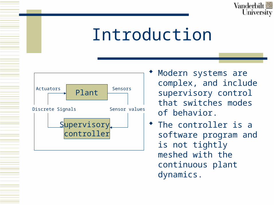
Modern systems are complex, and include supervisory control that switches modes of behavior.

The controller is a software program and is not tightly meshed with the continuous plant dynamics.

Plant

Supervisory controller

Actuators Sensors

Sensor valuesDiscrete Signals

Introduction

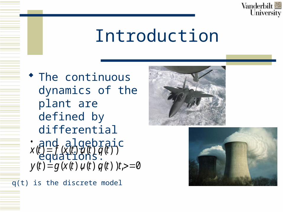
The continuous dynamics of the plant are defined by differential and algebraic equations.

0)),(),(),(()(

))(),(),(()(

ttqtutxgty

tqtutxftx

q(t) is the discrete model

Fault Detection and Isolation (FDI)

• The goal of this presentation is to briefly overview the study of FDI in hybrid systems with supervisory controllers.

• System faults may be component, actuator, sensor, and controller faults. (We do not deal with the later)

• The methodology we will cover combines qualitative and quantitative reasoning techniques to perform parameterized fault isolation of plant component faults.

Modeling for Diagnosis

Controller ModelPlant Model

Modeling for Diagnosis

Controller Model The primary model of the controller is

implemented as a finite state machine (FSM). States of the FSM correspond to the states of the

controller, which in turn define modes of the physical plant(q(t)).

The Transitions determine the conditions for switching states.

Modeling for DiagnosisController Model

1

3

2

4

5

6 7

8 9

10

t1t3

t2

t4 t5

t6

t7

t8

t9

t10

t11

Controller Model for 3 tank system

Tank 2

(C2)

Tank 2

(C2)

Tank 1

(C1)

= Valve

C = capacitance

R = resistance

Flow source 1 Flow source 2

R1 R6R2 R4

R3 R5Three Tank system

Modeling for Diagnosis

Plant Model Hybrid Bond Graph Models (HBG). State equations and temporal causal graph (TCG)

can be systematically derived from the bond graph representation of the system.

State equations along with the TCG constitute our diagnosis models.

Methodology for Hybrid Diagnosis

Hybrid observer: follows the continuous dynamics of the plant and identifies discrete mode changes.

Fault detection mechanism: signals a fault when the observer cannot compensate for differences between observed and expected behavior.

Fault isolation mechanism: generates candidate faults and refines them with the hybrid model and measurement from the system.

Methodology for Hybrid Diagnosis

Hybrid models

Diagnosismodels

System

Observer and modedetector

Fault isolation

Faultdetection

u y

r

^

y

Fault Hypotheses

The following information is assumed to be available to all modules:-HBG-FSA-FSM A = all possible autonomous events in the system-U = inputs-Y = system outputs-Parameters nominal

Diagnosis System Architecture

Methodology for Hybrid Diagnosis

Algorithm 1:Diagnosis Module

MODULE DIAGNOSE(Minitial,Xinitial)

// Observe the system until a fault is detected

<StackM, Yestimated>=OBSERVER(Minitial,Xinitial);

//Convert the quantitative residuals to qualitative values

QualResidualcurrent = SIGNAL_TO_SYMBOL(Y,Yestimated);

//Back propagate across modes to identify fault candidates

BackHorizon=2;

Listcandidates=HYBRID_BACK_PROP(StackM,QualResidualcurrent,BackHorizon);

//Forward propagete across modes to isolate the fault

Listcandidates=HYBRID_FAULT_OBSERVER(Listcandidates,Yestimated);

END DIAGNOSE

Hybrid Diagnosis Problem

Time Line

Mode 1 Mode 2 Mode 3

Mode 4

Mode 5Fault Occurs

Fault Detecte

d

Tracked TrajectoryActual Trajectory

T1 T2 T3 T4 T5 T6

Mode 6

Mode 7

Fault Hypothesis: <mode,parameter>

Piecewise linear hybrid dynamical systems

Presence of fault invalidates

tracked mode trajectory

Hypothesized fault mode

Known Controlled TransitionHypothesized

Autonomous Transition

Possible current modes

Hypothesized intermediate modes

Roll Back to find fault hypotheses

Roll Forward to confirm fault hypotheses

Catch up to current system mode to verify hypotheses against measurements

Note: Controller transitions known

Autonomous transitions have to be hypothesized

Fault IsolationBackground

The type of plant model employed determines the scheme to be employed.

Traditional schemes for the continuous domain use structured and directional residual approaches.

Extending these continuous methodologies to hybrid systems becomes intractable.

Fault Isolation

The approach we will follow involves hypotheses generation and hypotheses refinement.

Qualitative approach for hypotheses generation.

Qualitative-quantitative combined approach for hypotheses refinement.

Fault IsolationHypotheses Generation

For initial hypotheses generation we have to back propagate across modes. The assumption that the controller model is

correct implies that the observer predicted the correct mode sequence till the fault occurred. Therefore, the mode in which the fault occurred must be in the predicted trajectory of the observer.

Hypotheses GenerationTCG generation

•Effort and flow variables are vertices

•Relation between variables as directed edges

•=implies that two variables associated with the edge take on equal values, 1 implies direct proportionality,-1 implies inverse proportionality.

•Edge associated with component represents the component’s constituent relation.

Hypotheses GenerationAlgorithm 2:Hybrid Back Propagation

MODULE HYBRID_BACK_PROP(StackM, QualRi, BackHorizon)//Generate candidates in each mode in the mode trajectory. <Mcurrent, Timecurrent>=Pop(StackM); TCGcurrent=GET_TCG(HBG, Mcurrent)//Back propagate in selected mode for candidates in the mode Fcurrent=CONTINUOUS_BACK_PROP(TCGcurrent,QualRi); Add(Listcandidates,<Mcurrent,Timecurrent,Fcurrent>); Count=0;//Go back in the mode horizon upto BackHorizon number of nodes While(Count<BackHorizon)//Select next mode in mode trajectory and calculate TCG <Mnext, Timenext>=Pop(StackM); TCGnext, GET_TCG(HBG, Mnext);// Propagate qualitative deviations across modes QualRnext=BACK_PROP_ACROSS_MODES(Mcurrent, Mnext, QualRi)//Back propagate in selected mode for candidates in the mode Fnext=CONTINUOUS_BACK_PROP(TCGnext, QualRnext); Add(Listcandidates,<Mnext,Timenext,Fnext,1>); End While Return(Listcandidates)END MODULE

Roll Back Process

•Qualitative Hypotheses Generation• Back propagate through TCG in current mode to identify candidates

• Back propagate across mode transitions using transition conditions (need to account for reset conditions, and change in plant configuration – invert qualitatively)

• Repeat same process for previous modes to identify more candidates

- Tank 1 Pressure

- Tank 2 Pressure

- Tank 3 Pressure

Transition

Fault Occurred

Fault Detected

System Autonomous Transition

Fault IsolationHypotheses Refinement

First apply a qualitative forward propagation for each hypothesized fault candidate. To take into account mode changes, all possible modes

changes from the current mode are hypothesized. A candidate is dropped when the predictions do not

match the observations across all of the hypothesized modes

Apply a quantitative parameter estimation on remaining candidates. This approach works within a single continuous mode.

Hybrid Diagnosis Problem

Time Line

Mode 1 Mode 2 Mode 3

Mode 4

Mode 5Fault Occurs

Fault Detecte

d

Tracked TrajectoryActual Trajectory

T1 T2 T3 T4 T5 T6

Mode 6

Mode 7

Fault Hypothesis: <mode,parameter>

Piecewise linear hybrid dynamical systems

Presence of fault invalidates

tracked mode trajectory

Hypothesized fault mode

Known Controlled TransitionHypothesized

Autonomous Transition

Possible current modes

Hypothesized intermediate modes

Roll Back to find fault hypotheses

Roll Forward to confirm fault hypotheses

Catch up to current system mode to verify hypotheses against measurements

Note: Controller transitions known

Autonomous transitions have to be hypothesized

Quick Roll Forward

• Goal: Get to current mode, so parameter estimation can be applied to refine faults and identify fault magnitude

• Lemma 2: Sequence of k mode transitions in any order drives the system to the same final model

• Requires tracking of transients by progressive monitoringprogressive monitoring in continuous regions of space. Taylor series expansion defines qualitative fault signatures. Residual r(t) after fault can be described as:

• Progressive Monitoring: Match qualitative magnitude and slope of measurement signal transient against fault signature

)(!

)()(...

!2

)()(

!1

)()()()( 0

0

20

00

00 tRk

tttr

tttr

tttrtrtr k

kk

Fault signature: qualitative form of derivatives:

Qualitative form of

)(),....,(),( 000 trtrtr k

)(0),/()( 0 normalnormalbelowabovetr k

Quick Roll Forward

• In continuous case, mismatch implies fault hypothesis is not consistent. However, in hybrid tracking, it may imply that we are not in the right mode. We need to identify identify the current mode (roll forward)the current mode (roll forward)

• All controlled transitions are known, but we have to hypothesize autonomous transitions since observer can no longer predict them correctly

• Use fault signatures to hypothesize mode transitions

- Tank 1 Pressure

- Tank 2 Pressure

- Tank 3 Pressure

Transition

Fault Occurred

Fault Detected

System Autonomous Transition

Parameter Estimation (Real Time)

Derive transfer function model in current mode with only one unknown (fault parameter)

Initiate fault observer filter for each fault hypothesis least squares estimator for parameter estimation

Test for convergence identifies true fault candidate

Least Square Estimation from IOE

error prediction theis e output, estimated theis y

IOE),in sh' and svector(g'parameter theis

s,0' and sy' s,u' of madematrix a is

factor, forgetting theis ,covariance theis Q

)(ˆ)()()1()(

)(ˆ)()(ˆ

)1()()(ˆ

)()()1()(

1

tettQtt

tytyte

ttty

tttQtQT

T

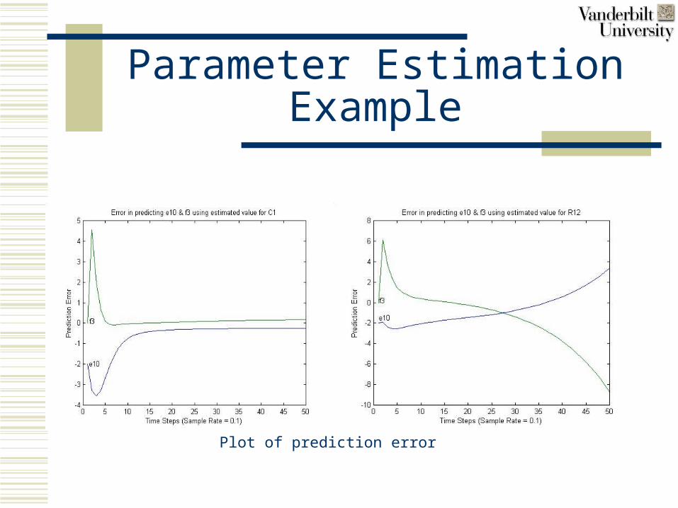
Parameter Estimation Example

Plot of prediction error

Quantitative Parameter Estimation: Issues

• Deriving the simplified one unknown parameter equation for least square estimator

• Convergence to local minima – need good initial estimates

• Need for persistent excitation in input – mitigated to some extent by reducing it to a one parameter estimation problem

• Measurement noise leads to biased estimates – need to apply more sophisticated techniques: IVM methodsObservation: What is good for qualitative FDI is not always good for quantitative identification using least squares methods

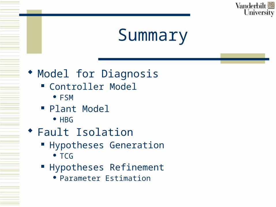
Summary

Model for Diagnosis Controller Model

FSM Plant Model

HBG

Fault Isolation Hypotheses Generation

TCG Hypotheses Refinement

Parameter Estimation

Conclusion

By having the supervisory controller model and assuming that our model is correct, we do not have to make the assumption that faults are detected in the mode in which they occur, and we still are able to avoid the intractability problem.

Combination of qualitative + quantitative approaches suitable for online diagnosis

Approach different from discrete-event approaches of Lunze and Sampath