Model-Based Design of a Plant-Wide Control Strategy …web.mit.edu/.../model_based_design_of_a_plantwide_control_strategy...Model-Based Design of a Plant-Wide Control Strategy for

Model-Based Design of a Plant-Wide Control Strategy for aContinuous Pharmaceutical Plant

Richard Lakerveld, Brahim Benyahia, Richard D. Braatz, and Paul I. BartonDept. of Chemical Engineering, Process Systems Engineering Laboratory,

Massachusetts Institute of Technology, Cambridge, MA 02139

DOI 10.1002/aic.14107Published online April 25, 2013 in Wiley Online Library (wileyonlinelibrary.com)

The design of an effective plant-wide control strategy is a key challenge for the development of future continuous phar-maceutical processes. This article presents a case study for the design of a plant-wide control structure for a systeminspired by an end-to-end continuous pharmaceutical pilot plant. A hierarchical decomposition strategy is used to clas-sify control objectives. A plant-wide dynamic model of the process is used to generate parametric sensitivities, whichprovide a basis for the synthesis of control loops. Simulations for selected disturbances illustrate that the critical qualityattributes (CQAs) of the final product can be kept close to specification in the presence of significant and persistent dis-turbances. Furthermore, it is illustrated how selected CQAs of the final product can be brought simultaneously to a newsetpoint while maintaining the remaining CQAs at a constant value during this transition. The latter result shows flexi-bility to control CQAs independently of each other. VC 2013 American Institute of Chemical Engineers AIChE J, 59:

3671–3685, 2013

Keywords: process control, design (process simulation), plant-wide control, continuous pharmaceutical manufacturing,sensitivity analysis

Introduction

The pharmaceutical industry is historically dominated bybatchwise processing. However, the industry is challengedby demands for faster time-to-market, tighter control overproduct quality, and a smaller ecological foot print. Continu-ous manufacturing could potentially improve the perform-ance of pharmaceutical processes, as continuous processesare preferred for certain types of chemistry (e.g., see Refs 1–4),increased efficiency through material and energy recycling,and increased predictability when combined with real-timemonitoring of process and product quality. Cases have beenreported where significant cost savings can be achieved forcontinuous manufacturing compared to batchwise manufac-turing.5–13 Consequently, there is a strong interest fromindustry to investigate the potential benefits of new continu-ous pharmaceutical processes.6,8 For example, Robergeet al.7 estimated that about 50% of the reactions theyanalyzed that were running at Lonza would benefit fromcontinuous processes. However, the transition toward con-tinuous pharmaceutical processing poses new challengesthat need to be addressed. A key challenge is the design ofan effective control strategy for continuous pharmaceuticalmanufacturing, which has to optimize the performance ofthe plant as a whole instead of isolated unit operations.

Specific features of pharmaceutical processes have to be takeninto account when approaching this challenge. Pharmaceuticalprocesses are typically characterized by a large variety of unitoperations to manufacture a pharmaceutical product, whichcan easily result in complicated dynamic behavior once theprocesses are connected. Furthermore, instead of relying onfixed recipes as is typically done in batchwise processing, thechallenge for control of continuous pharmaceutical processingis to actively maintain the system within a safe region ofoperation to support regulatory requirements. Disturbancesthat act on the process can force the system outside the saferegion of operation, which has to be prevented by an effectiveplant-wide control strategy.

Plant-wide control is concerned with the design of a con-trol structure for a complete plant. The study of synthesis ofplant-wide control systems for continuous manufacturingplants has a long history. The questions to be answered con-cern which variables to measure, manipulate, and controland how to connect them. Buckley14 introduces the conceptof plant-wide material-balance control by distinguishingbetween the direction in which the inventories of intermedi-ate storage vessels are controlled. Several groups have pro-posed systematic procedures for the design of plant-widecontrol structures. Morari et al.15,16 approached the system-atic development of plant-wide control by introducing a mul-tilayer-multiechelon concept to decompose the controlproblem into a temporal component by classifying disturban-ces and a topological component by aggregating interactinggroups of processing units with a well-specified operationalobjective. Temporal classification of disturbances helps to

Additional Supporting Information may be found in the online version of thisarticle.

Correspondence concerning this article should be addressed to P. I. Barton [email protected].

VC 2013 American Institute of Chemical Engineers

AIChE Journal 3671October 2013 Vol. 59, No. 10

split the control task into an optimizing and a regulatingcomponent. Topological classification of the process reducesthe complexity of the overall control problem. Larsson andSkogestad17 proposed a top-down analysis to select con-trolled variables followed by a bottom-up synthesis of thecontrol loops. Stephanopoulos and Ng18 proposed to use ahierarchical view of a plant, such as developed by Douglas19

for process synthesis, to facilitate decision making for thedesign of plant-wide control structures. A hierarchical viewdecomposes the complexity of the plant-wide control designproblem and naturally distributes design tasks over differenthierarchical views based on the time scales involved. Theseparation of time scales has been demonstrated to be benefi-cial for the design of plant-wide control structures.20 Thedecomposition of a process into different hierarchical viewsis particularly of interest for continuous pharmaceutical proc-esses as a result of the complexity and various sections forproduction and purification of intermediates, and formulationof the final drug product.

Control strategies for continuous pharmaceutical processeshave to be aligned with quality-by-design (QbD) concepts tomake the continuous pharmaceutical processes robust to dis-turbances, uncertainties, and implementation errors. QbD forpharmaceutical processes involves the identification of criti-cal quality attributes (CQAs) and critical process parameters(CPPs).21 CQAs are properties of material in the process thatneed to be controlled within given bounds to ensure a finalproduct quality that is within specification. CPPs are processinputs that have a strong influence on CQAs. Typically, theso-called design space is defined, which is the range of val-ues of all critical process inputs (i.e., input variables andprocess parameters) for which the process is known to give aproduct of sufficient quality.22 Challenges for the proper useof a design space involve the cost of defining the designspace and limited applicability during scale-up.23 A highdimension of the design space often prohibits an exhaustiveexploration of the design space, which can result in reducedflexibility for operation, that is, certain combinations of pa-rameters would give a product of sufficient quality, but arenot part of the design space because the favorable outcomehas not been proven a priori. Therefore, active control ofproduct properties via feedback and process analytical toolsinstead of an exhaustive documentation of a design spacemay well be a more efficient way to develop pharmaceuticalprocesses.23 Such active control is likely to be more relevantfor continuous pharmaceutical manufacturing because dy-namics play a more profound role for integrated continuousprocesses compared to the dynamics of a chain of individualbatch processes. Recently, it was demonstrated, for example,that active feedback control is efficient for a continuouspharmaceutical tablet manufacturing process via rollercompaction.24

The aim of this article is to demonstrate the model-baseddesign of a plant-wide control strategy for an end-to-endcontinuous pharmaceutical pilot plant using active feedbackcontrol. The system is inspired by a pilot plant that has beenbuilt within the Novartis-MIT Center for Continuous Manu-facturing and produces a pharmaceutical product from start(synthesis of intermediates) to finish (coating of drug prod-uct) in a fully continuous fashion. However, the system doesnot mimic the real plant exactly. For example, some featuressuch as recycling were not implemented in the real plant.The control strategy aims to exploit hierarchical decomposi-tion to reduce the complexity of the problem and to

minimize disturbance propagation between various sectionsof the plant. A model-based systems approach is of key im-portance for the development of future continuous pharma-ceutical processes.25–27 Therefore, a plant-wide dynamicmodel of the pilot plant28 was used to evaluate systemati-cally the influence of CPPs on selected CQAs at each levelof the hierarchical decomposition by evaluating parametricsensitivities, which forms the basis for selecting controlloops. The resulting control strategy ensures that both plant-wide and local control objectives are effectively addressedwith minimum interference due to the hierarchical nature ofthe control strategy.

The article is organized as follows. First, the continuouspharmaceutical pilot plant used as a case study in thiswork is described. The hierarchical decomposition of theprocess is discussed in the subsequent section includingthe selection of the control loops at each level of thedecomposition. The control strategy is implemented in adynamic model, which is used in the Model-Based Imple-mentation of the Control Structure section to study theperformance of the control strategy for selected disturban-ces and setpoint changes.

Approach

Process description

A schematic representation of the pilot plant is given inFigure 1. The process consists of several reactions and separa-tions for synthesis and purification of intermediates and thefinal active pharmaceutical ingredient (API) followed by asequence of downstream units that produce a pharmaceuticalproduct in tablet form. The calibrated volumetric pumps canbe used directly as actuator and as flow indicator. Two reac-tants (C1;C2) are mixed at the beginning of the process in astatic mixer (M1) with a catalyst and recycled material. Themixture is fed to a tubular reactor (R1) operated at elevatedtemperature where the chemical reactions

C1 1 C2 $Cat1

C3 (1)

C1 ! I1 (2)

C3 ! I2 (3)

1

2C1 1

3

2C2 1

1

2C3 ! I3 (4)

occur with C3 being the desired intermediate compound forproduction of the final API and compounds I1; I2, and I3

being undesired byproducts. Reactions 1–4 are relativelyslow. An in-line instrument is available at the outlet of thereactor to measure the concentration of both reactants andthe intermediate using infrared spectroscopy. Two solvents(S1; S2) are added in a mixer (M2) at the outlet of the reactorto extract reactant C2 and the catalyst from the mixture. Thetwo phases are subsequently separated by a membrane sepa-rator (S1). Two flow meters are installed at the outlet of themembrane. The stream with reactant C2 and the catalyst issent to waste and the stream with the remaining compoundsis introduced into a crystallizer (Cr1) operating at low-tem-perature to crystallize the desired intermediate compound C3.An antisolvent (S3) is added to the first crystallizer (Cr1) tolower the solubility of compound C3. A second crystallizer(Cr2) operated at lower-temperature is used to increase yield.Both crystallizers are equipped with a level sensor and alocal temperature controller, which maintains the temperature

3672 DOI 10.1002/aic Published on behalf of the AIChE October 2013 Vol. 59, No. 10 AIChE Journal

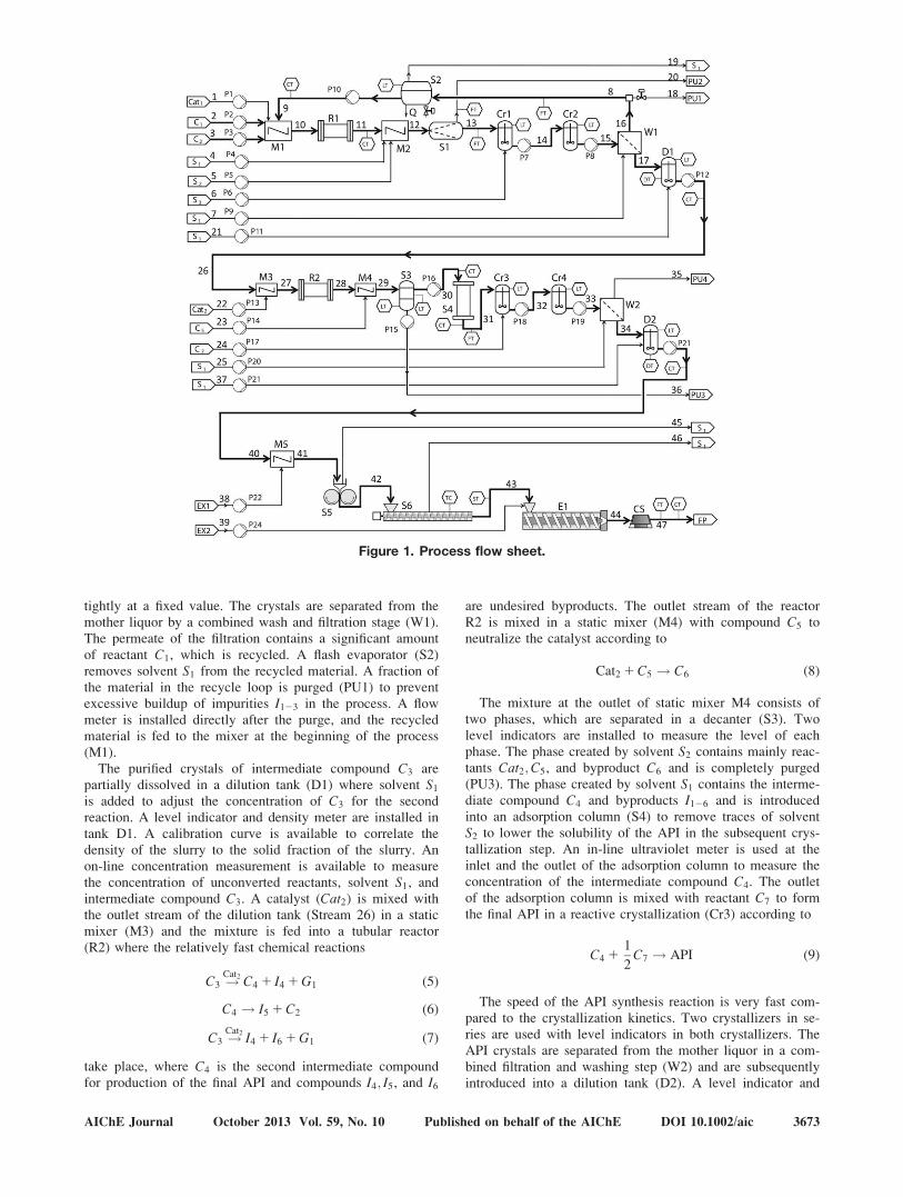
tightly at a fixed value. The crystals are separated from themother liquor by a combined wash and filtration stage (W1).The permeate of the filtration contains a significant amountof reactant C1, which is recycled. A flash evaporator (S2)removes solvent S1 from the recycled material. A fraction ofthe material in the recycle loop is purged (PU1) to preventexcessive buildup of impurities I123 in the process. A flowmeter is installed directly after the purge, and the recycledmaterial is fed to the mixer at the beginning of the process(M1).

The purified crystals of intermediate compound C3 arepartially dissolved in a dilution tank (D1) where solvent S1

is added to adjust the concentration of C3 for the secondreaction. A level indicator and density meter are installed intank D1. A calibration curve is available to correlate thedensity of the slurry to the solid fraction of the slurry. Anon-line concentration measurement is available to measurethe concentration of unconverted reactants, solvent S1, andintermediate compound C3. A catalyst (Cat2) is mixed withthe outlet stream of the dilution tank (Stream 26) in a staticmixer (M3) and the mixture is fed into a tubular reactor(R2) where the relatively fast chemical reactions

C3 !Cat2

C4 1 I4 1 G1 (5)

C4 ! I5 1 C2 (6)

C3 !Cat2

I4 1 I6 1 G1 (7)

take place, where C4 is the second intermediate compoundfor production of the final API and compounds I4; I5, and I6

are undesired byproducts. The outlet stream of the reactorR2 is mixed in a static mixer (M4) with compound C5 toneutralize the catalyst according to

Cat2 1 C5 ! C6 (8)

The mixture at the outlet of static mixer M4 consists oftwo phases, which are separated in a decanter (S3). Twolevel indicators are installed to measure the level of eachphase. The phase created by solvent S2 contains mainly reac-tants Cat2;C5, and byproduct C6 and is completely purged(PU3). The phase created by solvent S1 contains the interme-diate compound C4 and byproducts I126 and is introducedinto an adsorption column (S4) to remove traces of solventS2 to lower the solubility of the API in the subsequent crys-tallization step. An in-line ultraviolet meter is used at theinlet and the outlet of the adsorption column to measure theconcentration of the intermediate compound C4. The outletof the adsorption column is mixed with reactant C7 to formthe final API in a reactive crystallization (Cr3) according to

C4 11

2C7 ! API (9)

The speed of the API synthesis reaction is very fast com-pared to the crystallization kinetics. Two crystallizers in se-ries are used with level indicators in both crystallizers. TheAPI crystals are separated from the mother liquor in a com-bined filtration and washing step (W2) and are subsequentlyintroduced into a dilution tank (D2). A level indicator and

Figure 1. Process flow sheet.

AIChE Journal October 2013 Vol. 59, No. 10 Published on behalf of the AIChE DOI 10.1002/aic 3673

density meter are installed in the dilution tank. A calibrationcurve is available to correlate the density of the slurry to thesolid content of the slurry and an on-line concentration mea-surement is available to measure the concentration of uncon-verted reactants, solvent S1, and API. The slurry with APIcrystals is mixed (M5) with an excipient (EX1) to improveflowability of the powder. Drying consists of two steps. First,the bulk of the solvent is removed in a double drum dryer(S5). Subsequently, the solvent content of the powder isbrought to a lower value in a screw dryer (S6). The solventcontent is measured at the outlet of the screw dryer by anear-infrared (NIR) probe. The dried powder is mixed with asecond excipient (EX2) to improve the stability of the finaltablet. The excipient is dosed with a gravimetric feeder(P24). The mixture is fed to an extruder with a mold (E1) toshape the mixture into a tablet form. A decomposition reac-tion of the final API occurs within the extruder according to

API ! I7 1 C2 (10)

The production of the tablet is finalized by adding a layerof coating material in a continuous coating station. A NIRprobe is installed at the end of the process to measure thesolvent content, total impurity content, and API dosage ofthe final tablets. Finally, the production rate of the finalproduct is measured.

Model

A dynamic model of the pilot plant has been developed tosystematically evaluate sensitivities between CPPs and CQAsand to test the performance of various control structures forselected disturbances. The model has been described in detailelsewhere.28 A summary of the model including physicalproperties of the system studied, and nominal operating condi-tions are given in Supporting Information for completeness.The values of the parameters are either obtained from experi-mental data or typical values are assumed. The precise valuesof model parameters are typically not critical to the perform-ance of a certain control structure.29 The core structure of themodel is based on mass, energy, and moment balances thataim for at least qualitatively correct behavior, which supportsthe synthesis and testing of a plant-wide control structure.

Hierarchical Decomposition and ControlObjectives

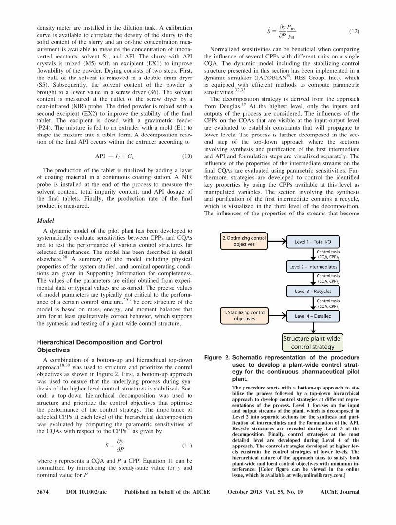
A combination of a bottom-up and hierarchical top-downapproach18,30 was used to structure and prioritize the controlobjectives as shown in Figure 2. First, a bottom-up approachwas used to ensure that the underlying process during syn-thesis of the higher-level control structures is stabilized. Sec-ond, a top-down hierarchical decomposition was used tostructure and prioritize the control objectives that optimizethe performance of the control strategy. The importance ofselected CPPs at each level of the hierarchical decompositionwas evaluated by computing the parametric sensitivities ofthe CQAs with respect to the CPPs31 as given by

S 5@y

@P(11)

where y represents a CQA and P a CPP. Equation 11 can benormalized by introducing the steady-state value for y andnominal value for P

S 5@y

@P

Pnv

yst

(12)

Normalized sensitivities can be beneficial when comparingthe influence of several CPPs with different units on a singleCQA. The dynamic model including the stabilizing controlstructure presented in this section has been implemented in adynamic simulator (JACOBIAN

VR

, RES Group, Inc.), whichis equipped with efficient methods to compute parametricsensitivities.32,33

The decomposition strategy is derived from the approachfrom Douglas.19 At the highest level, only the inputs andoutputs of the process are considered. The influences of theCPPs on the CQAs that are visible at the input-output levelare evaluated to establish constraints that will propagate tolower levels. The process is further decomposed in the sec-ond step of the top-down approach where the sectionsinvolving synthesis and purification of the first intermediateand API and formulation steps are visualized separately. Theinfluence of the properties of the intermediate streams on thefinal CQAs are evaluated using parametric sensitivities. Fur-thermore, strategies are developed to control the identifiedkey properties by using the CPPs available at this level asmanipulated variables. The section involving the synthesisand purification of the first intermediate contains a recycle,which is visualized in the third level of the decomposition.The influences of the properties of the streams that become

Figure 2. Schematic representation of the procedureused to develop a plant-wide control strat-egy for the continuous pharmaceutical pilotplant.

The procedure starts with a bottom-up approach to sta-

bilize the process followed by a top-down hierarchical

approach to develop control strategies at different repre-

sentations of the process. Level 1 focuses on the input

and output streams of the plant, which is decomposed in

Level 2 into separate sections for the synthesis and puri-

fication of intermediates and the formulation of the API.

Recycle structures are revealed during Level 3 of the

decomposition. Finally, control strategies at the most

detailed level are developed during Level 4 of the

approach. The control strategies developed at higher lev-

els constrain the control strategies at lower levels. The

hierarchical nature of the approach aims to satisfy both

plant-wide and local control objectives with minimum in-

terference. [Color figure can be viewed in the online

issue, which is available at wileyonlinelibrary.com.]


wileyonlinelibrary.com

available in this level on the control objectives of this sec-tion are analyzed and suitable control strategies are devel-oped. For this study, the control objective is to minimize thepropagation of disturbances that are acting on the recycle toCQAs at a higher level of the decomposition. Finally, theprocess is fully represented in the fourth level of the decom-position where remaining degrees of freedom can be used tosatisfy local control objectives. The time constants of the rel-evant processes at higher levels are slow and steady-state in-formation can be used, whereas dynamic modeling has to beused at the lowest level to evaluate rejection of faster distur-bances. The final control structure of the continuous pharma-ceutical pilot plant is obtained by combining eachsynthesized control layer in a single control structure. A gen-eral description of all the steps involved during the applica-tion of the design procedure as illustrated in Figure 2 isprovided as Supporting Information. The application of theproposed strategy to the described pilot plant is discussed inmore detail in the subsequent sections.

Stabilizing control structure

The stabilizing control layer is obtained by identifying allintegrating processes and subsequently by synthesizing con-trol loops that stabilize these integrating processes, whichinvolves all of the tanks with an attached pump. The outletflow rates are used to control the levels of the tanks, as theinlet flow rate is difficult to manipulate for several of thetanks. As a result, the feed flow rates of the process aredegrees of freedom for the synthesis of the plant-wide con-trol strategy. Table 1 gives an overview of all control loopsthat are part of the stabilizing control layer. All level con-trollers use proportional-control only. The tuning of thecontrol loops will be discussed in the section involving thesynthesis of the most detailed control layer (Level 4). Forthe first three levels of the decomposition strategy, onlysteady-state sensitivities are analyzed to synthesize thehigher-level control loops. The tuning of the level controllersof the stabilizing control layer has little influence on thesteady-state behavior of the system.

Level 1: Input/output

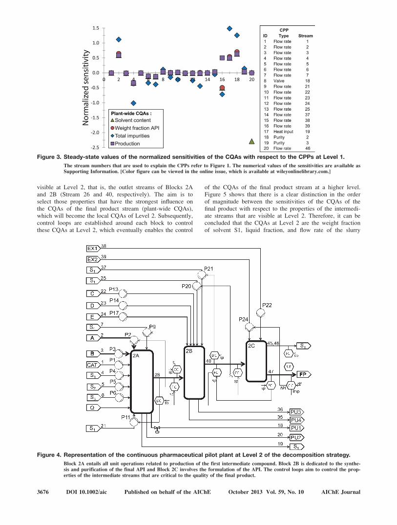
The CQAs that are visible at the input-output level aregiven in Table 2 and contain the requirements for the tablets.The CPPs that can influence the CQAs at this level are thecomposition and flow rates of all the remaining streams. Fig-ure 3 depicts the computed sensitivities of the CQAs atsteady state with respect to the CPPs that are visible at Level1. The large time constant of the process representation atLevel 1 warrants the use of sensitivities at steady state only.The results from Figure 3 can be used to rank the CPPs that

have a steady-state effect on the CQAs of the final product,which preferentially are used in subsequent levels to satisfylong-term control objectives. The CPPs that do not have asignificant effect on the long-term behavior of the processare preferentially used to satisfy local control objectives atmore detailed levels of representation of the process. Thesolvent content and the API dosage of the final tablets andthe production rate are mainly influenced by the flow rate ofreactant C1, flow rate of solvent S1 for the first extraction,flow rate of the second excipient, heat input to the flashevaporator, and purity of the feed stream. The CPPs thathave a strong influence on solvent content, API dosage, andproduction rate also have a strong influence on the total levelof impurities of the final tablets. In addition, the purity ofthe final tablets is significantly influenced by most of theother CPPs that are visible at Level 1 of the decomposition,which likely makes the control of the purity of the final tab-lets most challenging in subsequent levels. Finally, the anal-ysis confirms that the solvent content of the final tablets isstrongly and selectively influenced by the flow rate of sol-vent S1 of Stream 46. Note that the CPPs evaluated in Figure3 can be used as manipulated variables within their designspace to control the CQAs of the final product with excep-tion of the purity of the feeding materials, which is not apractical manipulated variable. This analysis does, however,stress the importance of monitoring changes in the composi-tion of the feed materials, which are quite common, forexample, due to variations in feed material lots or due tovariations between suppliers of feed materials. At Level 1 ofthe decomposition, no direct control loops are establishedbetween inputs and outputs as there can potentially be largetime delays between controlled and manipulated variables,which will result in sluggish behavior. Instead, control loopsinvolving the important CPPs for long-term behavior areestablished at the next level to ensure sufficiently fast controlloops to manipulate the CQAs of the final product as dis-cussed in the next section.

Level 2: Intermediates and the formulation of the API

Figure 4 illustrates the process representation at Level 2of the decomposition. The first block (2A) contains all unitoperations that accomplish the synthesis and purification ofthe first intermediate compound (C3). The second block (2B)is connected to Block 2A via Stream 26 and consists of allunit operations that transform the slurry with crystals of in-termediate compound C3 into a slurry with crystals of thefinal API (Stream 40). The final block (2C) represents allunit operations involved in the formulation of the API. Fig-ure 4 also contains the control loops that are established atthis level, which are the result of the analysis of parametricsensitivities with respect to the CPPs and CQAs that is per-formed at Level 2. Figure 5 depicts the normalized sensitiv-ities of the CQAs of the final product stream with respect tothe properties of the intermediate streams that become

Table 1. Control Loops of the Stabilizing Control Layer

Controlled Variable Manipulated Variable

VCr1 F14

VCr2 F15

VD1 F26

VS3;OR F30

VS3;AQ F36

VCr3 F32

VCr4 F33

VD2 F40

V refers to volume and F refers to flow rate. The abbreviations for unit oper-ations and stream numbers are indicated in Figure 1.

Table 2. Critical Quality Attributes of the Final Tablets

Critical Quality Attribute Allowable Range Unit

Primary CQAsSolvent content (0, 0.0050) g/gTotal level of impurities (0, 0.008) g/gDosage of API (0.42, 0.48) g/g

Secondary CQAProduction rate (0.22, 0.30) kg/h


visible at Level 2, that is, the outlet streams of Blocks 2Aand 2B (Stream 26 and 40, respectively). The aim is toselect those properties that have the strongest influence onthe CQAs of the final product stream (plant-wide CQAs),which will become the local CQAs of Level 2. Subsequently,control loops are established around each block to controlthese CQAs at Level 2, which eventually enables the control

of the CQAs of the final product stream at a higher level.Figure 5 shows that there is a clear distinction in the orderof magnitude between the sensitivities of the CQAs of thefinal product with respect to the properties of the intermedi-ate streams that are visible at Level 2. Therefore, it can beconcluded that the CQAs at Level 2 are the weight fractionof solvent S1, liquid fraction, and flow rate of the slurry

Figure 3. Steady-state values of the normalized sensitivities of the CQAs with respect to the CPPs at Level 1.

The stream numbers that are used to explain the CPPs refer to Figure 1. The numerical values of the sensitivities are available as

Supporting Information. [Color figure can be viewed in the online issue, which is available at wileyonlinelibrary.com.]

Figure 4. Representation of the continuous pharmaceutical pilot plant at Level 2 of the decomposition strategy.

Block 2A entails all unit operations related to production of the first intermediate compound. Block 2B is dedicated to the synthe-

sis and purification of the final API and Block 2C involves the formulation of the API. The control loops aim to control the prop-

erties of the intermediate streams that are critical to the quality of the final product.



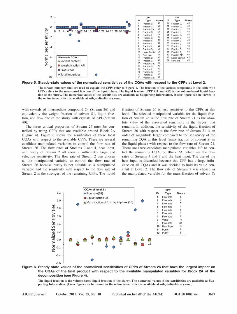
with crystals of intermediate compound C3 (Stream 26) andequivalently the weight fraction of solvent S1, liquid frac-tion, and flow rate of the slurry with crystals of API (Stream40).

The three critical properties of Stream 26 must be con-trolled by using CPPs that are available around Block 2A(Figure 4). Figure 6 shows the sensitivities of these localCQAs with respect to the available CPPs. There are severalcandidate manipulated variables to control the flow rate ofStream 26. The flow rates of Streams 2 and 4, heat input,and purity of Stream 2 all show a sufficiently large andselective sensitivity. The flow rate of Stream 2 was chosenas the manipulated variable to control the flow rate ofStream 26 because purity is not suitable as a manipulatedvariable and the sensitivity with respect to the flow rate ofStream 2 is the strongest of the remaining CPPs. The liquid

fraction of Stream 26 is less sensitive to the CPPs at thislevel. The selected manipulated variable for the liquid frac-tion of Stream 26 is the flow rate of Stream 21 as the abso-lute value of the associated sensitivity is the largest thatremains. In addition, the sensitivity of the liquid fraction ofStream 26 with respect to the flow rate of Stream 21 is anorder of magnitude larger compared to the sensitivity of theremaining CQA at this level (mass fraction of solvent S1 inthe liquid phase) with respect to the flow rate of Stream 21.There are three candidate manipulated variables left to con-trol the remaining CQA for Block 2A, which are the flowrates of Streams 4 and 7 and the heat input. The use of theheat input is discarded because this CPP has a large influ-ence on all CQAs and it was decided to hold its value con-stant at Level 2. The flow rate of Stream 7 was chosen asthe manipulated variable for the mass fraction of solvent S1

Figure 5. Steady-state values of the normalized sensitivities of the CQAs with respect to the CPPs at Level 2.

The stream numbers that are used to explain the CPPs refer to Figure 1. The fraction of the various compounds in the table with

CPPs refers to the mass-based fraction of the liquid phase. The liquid fraction (CPP #11 and #33) is the volume-based liquid frac-

tion of the slurry. The numerical values of the sensitivities are available as Supporting Information. [Color figure can be viewed in

the online issue, which is available at wileyonlinelibrary.com.]

Figure 6. Steady-state values of the normalized sensitivities of CPPs of Stream 26 that have the largest impact onthe CQAs of the final product with respect to the available manipulated variables for Block 2A of thedecomposition (see Figure 4).

The liquid fraction is the volume-based liquid fraction of the slurry. The numerical values of the sensitivities are available as Sup-

porting Information. [Color figure can be viewed in the online issue, which is available at wileyonlinelibrary.com.]




in the liquid phase of Stream 26, which yields a slightly bet-ter sensitivity compared to using the flow rate of Stream 4.Often several different choices can be made that lead to dif-ferent control structures. In general, the aim of plant-widecontrol is not to deliver a single optimized control structure,as there is always sufficient model uncertainty that it isimpossible to know for certain which control structure wouldbe optimal for the true plant. Different users can come todifferent control structures that can also be viable choices.At the very least, a good plant-wide control methodologyshould avoid generating control structures that will result inbad closed-loop performance due to poor pairings of varia-bles or conflicting local and plant-wide control objectives.

The qualitative results in Figure 6 are similar to the resultsin Figure 3 for the CPPs that are evaluated in both graphs.The reason for this similarity is that a variation in a CPPdepicted in both figures has to influence the CQAs of Stream26 first before this variation propagates to the CQAs of thefinal product. This observation can be generalized to any dis-turbance that occurs in the first section of the process (i.e.,in Block 2A), and the general strategy is to attenuate distur-bances such that the influence of the disturbances on localCQAs that have the most effect on the final product is mini-mized, which prevents upstream disturbances propagatingthrough the whole process. This strategy will be repeated inthe next level of the decomposition, which will create

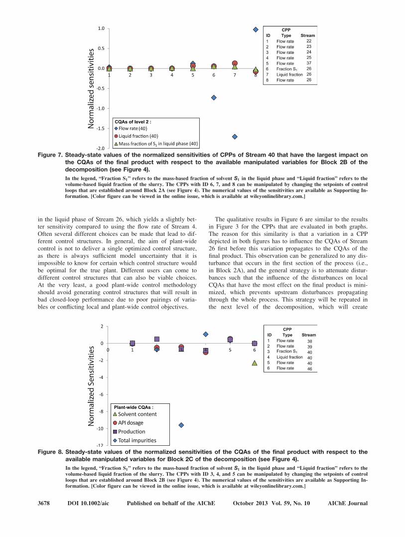
Figure 7. Steady-state values of the normalized sensitivities of CPPs of Stream 40 that have the largest impact onthe CQAs of the final product with respect to the available manipulated variables for Block 2B of thedecomposition (see Figure 4).

In the legend, “Fraction S1” refers to the mass-based fraction of solvent S1 in the liquid phase and “Liquid fraction” refers to the

volume-based liquid fraction of the slurry. The CPPs with ID 6, 7, and 8 can be manipulated by changing the setpoints of control

loops that are established around Block 2A (see Figure 4). The numerical values of the sensitivities are available as Supporting In-

formation. [Color figure can be viewed in the online issue, which is available at wileyonlinelibrary.com.]

Figure 8. Steady-state values of the normalized sensitivities of the CQAs of the final product with respect to theavailable manipulated variables for Block 2C of the decomposition (see Figure 4).

In the legend, “Fraction S1” refers to the mass-based fraction of solvent S1 in the liquid phase and “Liquid fraction” refers to the

volume-based liquid fraction of the slurry. The CPPs with ID 3, 4, and 5 can be manipulated by changing the setpoints of control

loops that are established around Block 2B (see Figure 4). The numerical values of the sensitivities are available as Supporting In-

formation. [Color figure can be viewed in the online issue, which is available at wileyonlinelibrary.com.]




another layer of protection against prolonged propagation ofdisturbances around Block 2A.

The sensitivities of the three CQAs that have to be con-trolled around Block 2B (see Figure 4) with respect to theavailable CPPs are illustrated in Figure 7. The CPPs that areavailable to control these CQAs are the flow rates of allinput streams into Block 2B that were also already visible inLevel 1 of the decomposition supplemented with the threeCQAs of Stream 26 that are input for Block 2B. Using anyof these CQAs from Block 2A as a manipulated variable tocontrol the CQAs out of Block 2B would involve changingthe setpoints of the control loops that are previously estab-lished around Block 2A. Figure 7 shows that several CPPsare suitable, that is, sufficiently large and selective, to con-trol the flow rate of Stream 40. The flow rate of Stream 26has been chosen as the manipulated variable to control theflow rate of Stream 40. The use of the liquid fraction ormass fraction of solvent S1 in Stream 26 as the manipulatedvariable to control the flow rate of Stream 40 would be fea-sible, but the control loops around Block 2A that controlthese two properties of Stream 26 are expected to saturateeasily, which makes the flow rate of Stream 26 a more suita-ble choice. The flow rate of Stream 37 has been chosen tocontrol the liquid fraction of Stream 40 as the sensitivity ofthis pair of CQA-CPP is an order of magnitude larger thanthe sensitivity of the mass fraction of solvent S1 in the liquidphase of Stream 40 (remaining CQA) with respect to theflow rate of Stream 37. A similar argument is the basis forselecting the flow rate of Stream 25 as the manipulated

variable to control the mass fraction of solvent S1 in the liq-uid phase of Stream 40 as this sensitivity is at least an orderof magnitude larger than the sensitivity of the other CQAswith respect to the same CPP.

Finally, suitable manipulated variables for the CQAs ofBlock 2C (see Figure 4) have to be identified. The sensitiv-ities of these CQAs with respect to the CPPs that are avail-able around Block 2C are given in Figure 8. Note that theCQAs of Block 2B are inputs for Block 2C and the setpointsof the control loops that are established as discussed in theprevious section can potentially be used to manipulate theCQAs of Block 2C. The level of total impurities of the finalproduct shows a large sensitivity with respect to the mass-based fraction of solvent S1 in the liquid phase of Stream40, which makes this CPP a suitable choice to establish acontrol loop around Block 2C to control the level of totalimpurities in the final product. Note that the sensitivity ofthe remaining CQAs with respect to this CPP is low. Simi-larly, the flow rate of Stream 46 is selective to control thesolvent content of the final product. The associated controllaw involving the solvent content and the flow rate of Stream46 cannot be finalized at this level of the decomposition assuitable actuators are not yet visible, but the control objec-tive that is established at Level 2 will constrain the choicesfor control loops that can be made at the most detailed levelof the decomposition. The two remaining CQAs aroundBlock 2C, that is, the final API dosage and production rate,show a similar order of magnitude of the sensitivities withrespect to the remaining CQAs. Therefore, two CPPs areselected to control those two CQAs, and the different prior-ities between them are used to establish the control laws.The sensitivities of these two remaining CQAs with respectto both the flow rate of Stream 39 and Stream 40 have a rea-sonably high value. The API dosage of the final tablets isconsidered to be of a higher priority (see Table 2) comparedto maintaining the production rate. The flow rate of Stream39 is expected to be a better manipulated variable comparedto the flow rate of Stream 40 as the time delay between achange in flow rate of Stream 39 and the time at which achange in one of the CQAs is observed is expected to beshorter and is, therefore, selected as the manipulated variableto control the final API dosage of the tablets around Block2C. Consequently, the flow rate of Stream 40 is selected asthe manipulated variable for controlling the production flowrate, which completes the design of the control structure atLevel 2 of the decomposition. The control loops that areestablished at this level are shown in Figure 4.

Level 3: Recycle structure

A control strategy around recycles is developed in Level 3of the decomposition procedure, which for this applicationinvolves expanding Block 2A from Level 2 of the decompo-sition to reveal the flows that constitute the recycle (seeFigure 9). The chosen control strategy aims to reject distur-bances within the recycle so as to prevent the propagation ofthese disturbances to the CQAs of a higher level. The firststep is to determine the properties of the streams that arevisible at Level 3 and have the largest impact on the CQAsrelated to Stream 26 as determined at Level 2 of the decom-position. Figure 10 shows the sensitivities of the CQAs ofStream 26 with respect to the weight fractions of the com-pounds and flow rates of Streams 9 and 11. Note that theproperties of Streams 9 and 11 cannot be treated as

Figure 9. Representation of the continuous pharma-ceutical pilot plant at Level 3 of the decom-position strategy.

Block 2A from Level 2 (see Figure 4) has been

expanded to visualize the recycle structure. Block 3A

contains all unit operations related to the first reaction,

which produces the intermediate impurity I1. Block 3B

represents all unit operations that are used to separate

the reaction products into a stream that is rich in impu-

rity I1 (Stream 26) and a stream that is rich in reactant

C1 (Stream 16), which is partially purged (Stream 18)

and send to a flash evaporator (Block 3C) to remove

solvent S1 (Stream 19) before the material returns to

the reaction section (Stream 9). The control loops aim

to control the CQAs of the streams that constitute the

recycle to minimize the propagation of disturbances to

the CQAs of Stream 26, which are critical at a higher

level of the decomposition.


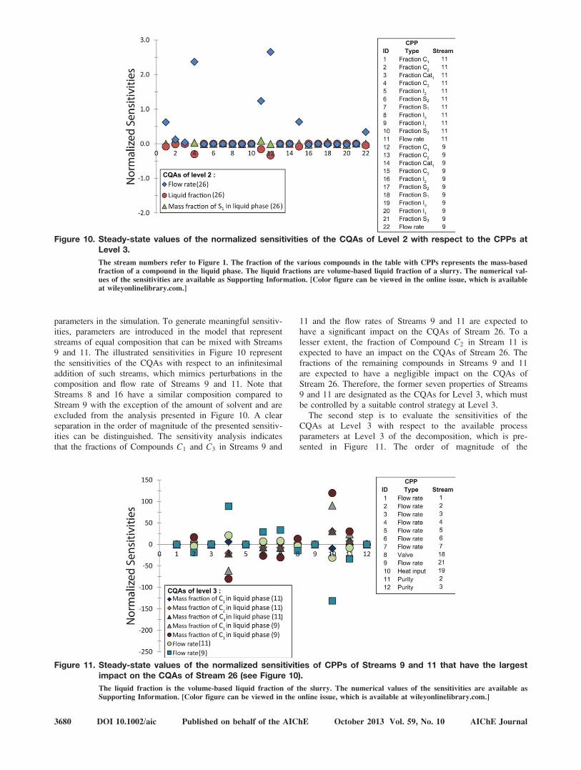
parameters in the simulation. To generate meaningful sensitiv-ities, parameters are introduced in the model that representstreams of equal composition that can be mixed with Streams9 and 11. The illustrated sensitivities in Figure 10 representthe sensitivities of the CQAs with respect to an infinitesimaladdition of such streams, which mimics perturbations in thecomposition and flow rate of Streams 9 and 11. Note thatStreams 8 and 16 have a similar composition compared toStream 9 with the exception of the amount of solvent and areexcluded from the analysis presented in Figure 10. A clearseparation in the order of magnitude of the presented sensitiv-ities can be distinguished. The sensitivity analysis indicatesthat the fractions of Compounds C1 and C3 in Streams 9 and

11 and the flow rates of Streams 9 and 11 are expected tohave a significant impact on the CQAs of Stream 26. To alesser extent, the fraction of Compound C2 in Stream 11 isexpected to have an impact on the CQAs of Stream 26. Thefractions of the remaining compounds in Streams 9 and 11are expected to have a negligible impact on the CQAs ofStream 26. Therefore, the former seven properties of Streams9 and 11 are designated as the CQAs for Level 3, which mustbe controlled by a suitable control strategy at Level 3.

The second step is to evaluate the sensitivities of theCQAs at Level 3 with respect to the available processparameters at Level 3 of the decomposition, which is pre-sented in Figure 11. The order of magnitude of the

Figure 11. Steady-state values of the normalized sensitivities of CPPs of Streams 9 and 11 that have the largestimpact on the CQAs of Stream 26 (see Figure 10).

The liquid fraction is the volume-based liquid fraction of the slurry. The numerical values of the sensitivities are available as


Figure 10. Steady-state values of the normalized sensitivities of the CQAs of Level 2 with respect to the CPPs atLevel 3.

The stream numbers refer to Figure 1. The fraction of the various compounds in the table with CPPs represents the mass-based

fraction of a compound in the liquid phase. The liquid fractions are volume-based liquid fraction of a slurry. The numerical val-

ues of the sensitivities are available as Supporting Information. [Color figure can be viewed in the online issue, which is available

at wileyonlinelibrary.com.]




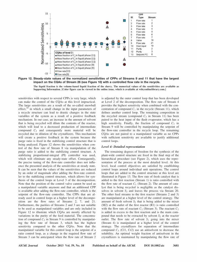
sensitivities with respect to several CPPs is very large, whichcan make the control of the CQAs at this level impractical.The large sensitivities are a result of the so-called snowballeffect,34 in which a small change in the input parameters ofa recycle structure can lead to drastic changes in the statevariables of the system as a result of a positive feedbackmechanism. In our case, an increase in the amount of solventthat is being recycled will dilute the contents of the reactor,which will lead to a decreased production of intermediatecompound C3 and consequently more material will berecycled due to dilution of the crystallizers. This mechanismwill create a positive feedback in the system because thepurge ratio is fixed in the stabilizing control structure that isbeing analyzed. Figure 12 shows the sensitivities when con-trol of the flow rate of Stream 8 via manipulation of thepurge ratio is added to the stabilizing control structure. Astabilizing proportional-integral (PI) controller was used,which will eliminate any steady-state offset. Consequently,the precise tuning of the flow-rate controller does not influ-ence the presented analysis of the sensitivities at steady state.It can be seen that the values of the sensitivities are reducedby an order of magnitude after adding the flow-rate control-ler to the stabilizing control structure, which allows for syn-thesis of the control loops at Level 3 of the decomposition.Note that the position of the control valve cannot be used asa manipulated variable anymore and that an additional CPPis available after adding the flow-rate controller, which is thesetpoint of the flow-rate controller. The CPPs that are al-ready used in control loops at a higher level of the decompo-sition are the flow rates of Streams 2, 7, and 21.Furthermore, the purities of Streams 2 and 3 are not suitableto be used as manipulated variables and are only included inFigure 12 to illustrate which CQAs are mostly affected byvariations in the purity of the feed material. The concentra-tion of compound C2 in Stream 9 is controlled by manipulat-ing the flow rate of Stream 3, which has the highestsensitivity compared to the other CQAs. Note that themanipulated variable for this control loop is the setpoint of aratio control loop, as a change in the required flow rate ofStream 3 can be anticipated when the flow rate of Stream 2

is adjusted by the outer control loop that has been developedat Level 2 of the decomposition. The flow rate of Stream 4provides the highest sensitivity when combined with the con-centration of compound C1 in the recycle (Stream 11), whichdefines another control loop. The remaining composition inthe recycled stream (compound C3 in Stream 11) has beenpaired to the heat input of the flash evaporator, which has ahigh sensitivity. Finally, the fraction of compound C3 inStream 9 will be controlled by manipulating the setpoint ofthe flow-rate controller in the recycle loop. The remainingCQAs are not paired to a manipulated variable as no CPPswith sufficient sensitivity are available to justify additionalcontrol loops.

Level 4: Detailed representation

The remaining degrees of freedom for the synthesis of theplant-wide control structure are fixed in the final step of thehierarchical procedure (see Figure 2), which uses the repre-sentation of the process at the most detailed level. At thislevel, local control objectives are satisfied by establishingcontrol loops around individual unit operations. The controlloops that are added to the control structure at this level areillustrated in Figure 13. The flow rate of fresh catalyst that isadded to the first reaction (Stream 1) is ratio controlled withthe flow rate of reactant C1 (Stream 2). The amount of cata-lyst that is being recycled is negligible as the catalyst dis-solves in solvent S2 and leaves the process via Stream 20.The other feed streams to the first reactor (Streams 2 and 3)are manipulated at a higher level of the control strategy. Theamount of fresh solvent S2 that is being added to the mixer(M2) at the outlet of the first reactor (R1) is ratio controlledwith the flow rate of reactant C2 (Stream 3). The reactant C2

is added in excess to the first reaction and is the main com-pound that needs to be extracted by solvent S2 at the reactoroutlet. The flow rate of solvent S1 going into the mixer(Stream 4) is manipulated at a higher level of the controlstrategy. The crystallizers for separation of intermediatecompound C3 (Cr1, Cr2) use an antisolvent to decrease thesolubility. An optimal weight fraction of antisolvent in thecrystallizers is maintained by manipulating the flow rate of

Figure 12. Steady-state values of the normalized sensitivities of CPPs of Streams 9 and 11 that have the largestimpact on the CQAs of Stream 26 (see Figure 10) with a controlled flow rate in the recycle.

The liquid fraction is the volume-based liquid fraction of the slurry. The numerical values of the sensitivities are available as




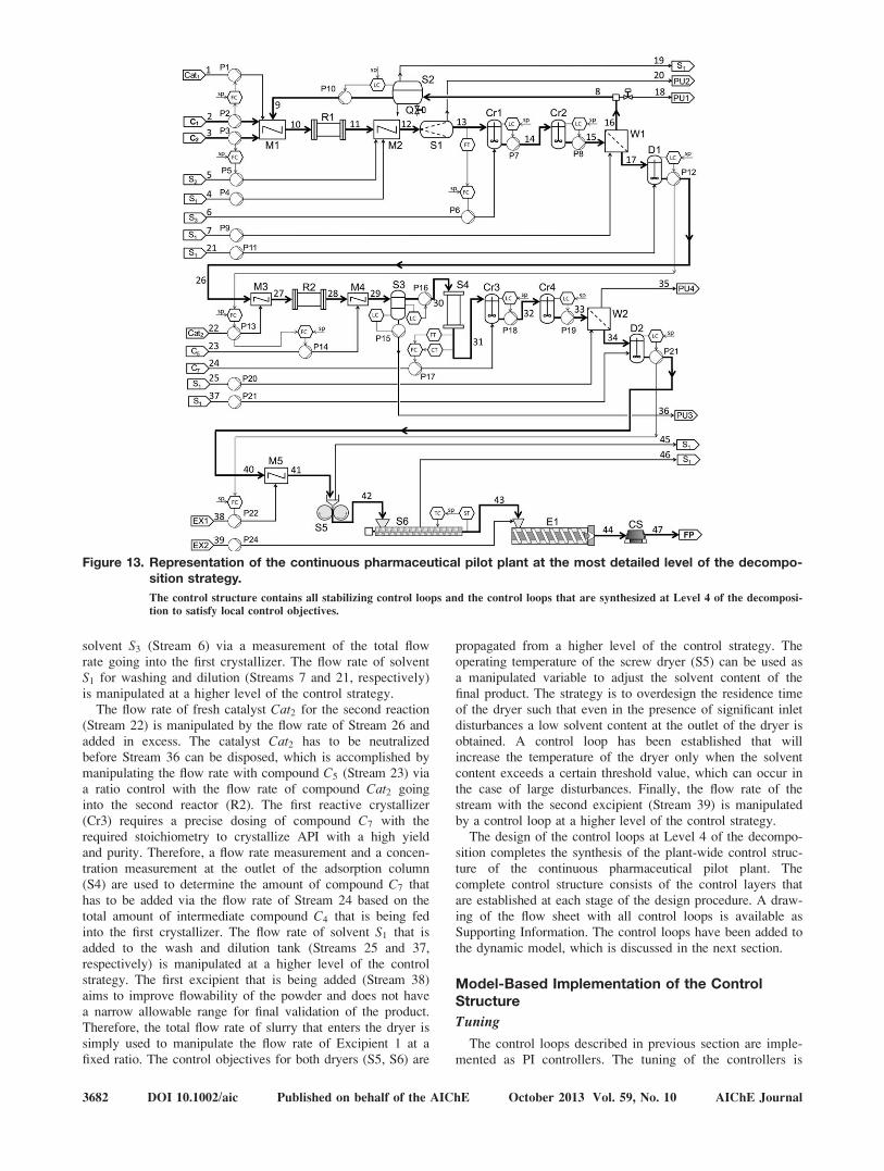
solvent S3 (Stream 6) via a measurement of the total flowrate going into the first crystallizer. The flow rate of solventS1 for washing and dilution (Streams 7 and 21, respectively)is manipulated at a higher level of the control strategy.

The flow rate of fresh catalyst Cat2 for the second reaction(Stream 22) is manipulated by the flow rate of Stream 26 andadded in excess. The catalyst Cat2 has to be neutralizedbefore Stream 36 can be disposed, which is accomplished bymanipulating the flow rate with compound C5 (Stream 23) viaa ratio control with the flow rate of compound Cat2 goinginto the second reactor (R2). The first reactive crystallizer(Cr3) requires a precise dosing of compound C7 with therequired stoichiometry to crystallize API with a high yieldand purity. Therefore, a flow rate measurement and a concen-tration measurement at the outlet of the adsorption column(S4) are used to determine the amount of compound C7 thathas to be added via the flow rate of Stream 24 based on thetotal amount of intermediate compound C4 that is being fedinto the first crystallizer. The flow rate of solvent S1 that isadded to the wash and dilution tank (Streams 25 and 37,respectively) is manipulated at a higher level of the controlstrategy. The first excipient that is being added (Stream 38)aims to improve flowability of the powder and does not havea narrow allowable range for final validation of the product.Therefore, the total flow rate of slurry that enters the dryer issimply used to manipulate the flow rate of Excipient 1 at afixed ratio. The control objectives for both dryers (S5, S6) are

propagated from a higher level of the control strategy. Theoperating temperature of the screw dryer (S5) can be used asa manipulated variable to adjust the solvent content of thefinal product. The strategy is to overdesign the residence timeof the dryer such that even in the presence of significant inletdisturbances a low solvent content at the outlet of the dryer isobtained. A control loop has been established that willincrease the temperature of the dryer only when the solventcontent exceeds a certain threshold value, which can occur inthe case of large disturbances. Finally, the flow rate of thestream with the second excipient (Stream 39) is manipulatedby a control loop at a higher level of the control strategy.

The design of the control loops at Level 4 of the decompo-sition completes the synthesis of the plant-wide control struc-ture of the continuous pharmaceutical pilot plant. Thecomplete control structure consists of the control layers thatare established at each stage of the design procedure. A draw-ing of the flow sheet with all control loops is available asSupporting Information. The control loops have been added tothe dynamic model, which is discussed in the next section.

Model-Based Implementation of the ControlStructure

Tuning

The control loops described in previous section are imple-mented as PI controllers. The tuning of the controllers is

Figure 13. Representation of the continuous pharmaceutical pilot plant at the most detailed level of the decompo-sition strategy.

The control structure contains all stabilizing control loops and the control loops that are synthesized at Level 4 of the decomposi-

tion to satisfy local control objectives.


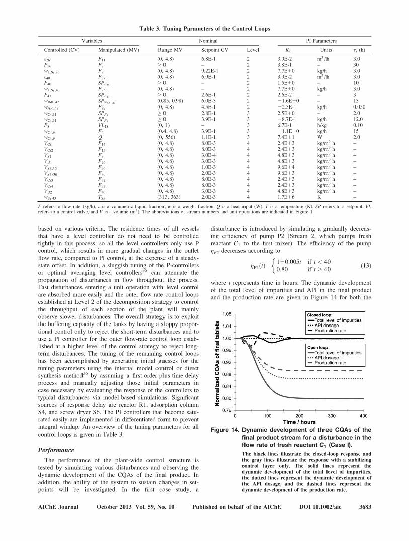
based on various criteria. The residence times of all vesselsthat have a level controller do not need to be controlledtightly in this process, so all the level controllers only use Pcontrol, which results in more gradual changes in the outletflow rate, compared to PI control, at the expense of a steady-state offset. In addition, a sluggish tuning of the P-controllersor optimal averaging level controllers35 can attenuate thepropagation of disturbances in flow throughout the process.Fast disturbances entering a unit operation with level controlare absorbed more easily and the outer flow-rate control loopsestablished at Level 2 of the decomposition strategy to controlthe throughput of each section of the plant will mainlyobserve slower disturbances. The overall strategy is to exploitthe buffering capacity of the tanks by having a sloppy propor-tional control only to reject the short-term disturbances and touse a PI controller for the outer flow-rate control loop estab-lished at a higher level of the control strategy to reject long-term disturbances. The tuning of the remaining control loopshas been accomplished by generating initial guesses for thetuning parameters using the internal model control or directsynthesis method36 by assuming a first-order-plus-time-delayprocess and manually adjusting those initial parameters incase necessary by evaluating the response of the controllers totypical disturbances via model-based simulations. Significantsources of response delay are reactor R1, adsorption columnS4, and screw dryer S6. The PI controllers that become satu-rated easily are implemented in differentiated form to preventintegral windup. An overview of the tuning parameters for allcontrol loops is given in Table 3.

Performance

The performance of the plant-wide control structure istested by simulating various disturbances and observing thedynamic development of the CQAs of the final product. Inaddition, the ability of the system to sustain changes in set-points will be investigated. In the first case study, a

disturbance is introduced by simulating a gradually decreas-ing efficiency of pump P2 (Stream 2, which pumps freshreactant C1 to the first mixer). The efficiency of the pumpgP2 decreases according to

gP2 tð Þ5 120:005t if t < 40

0:80 if t � 40

�(13)

where t represents time in hours. The dynamic developmentof the total level of impurities and API in the final productand the production rate are given in Figure 14 for both the

Table 3. Tuning Parameters of the Control Loops

Variables Nominal PI Parameters

Controlled (CV) Manipulated (MV) Range MV Setpoint CV Level Kc Units si (h)

e26 F11 (0, 4.8) 6.8E-1 2 3.9E-2 m3=h 3.0F26 F2 � 0 – 2 3.8E-1 – 30wL;S1 ;26 F7 (0, 4.8) 9.22E-1 2 7.7E10 kg/h 3.0e40 F37 (0, 4.8) 6.9E-1 2 3.9E-2 m3=h 3.0F40 SPF26

� 0 – 2 1.5E10 – 10wL;S1 ;40 F25 (0, 4.8) – 2 7.7E10 kg/h 3.0F47 SPF40

� 0 2.6E-1 2 2.6E-2 – 3wIMP;47 SPwL;S1 ;40

(0.85, 0.98) 6.0E-3 2 21.6E10 – 13wAPI;47 F39 (0, 4.8) 4.5E-1 2 22.5E-1 kg/h 0.050wC2 ;11 SPF3

� 0 2.8E-1 3 2.5E10 – 2.0wC3 ;11 SPF8

� 0 3.9E-1 3 28.7E-1 kg/h 12.0F8 VL18 (0, 1) – 3 6.7E-1 h/kg 0.10wC1 ;9 F4 (0.4, 4.8) 3.9E-1 3 21.1E10 kg/h 15wC3 ;9 Q (0, 556) 1.1E-1 3 7.4E11 W 2.0VCr1 F14 (0, 4.8) 8.0E-3 4 2.4E13 kg/m3 h –VCr2 F15 (0, 4.8) 8.0E-3 4 2.4E13 kg/m3 h –VS2 F9 (0, 4.8) 3.0E-4 4 4.8E13 kg/m3 h –VD1 F26 (0, 4.8) 3.0E-3 4 4.8E13 kg/m3 h –VS3;AQ F36 (0, 4.8) 1.0E-3 4 9.6E14 kg/m3 h –VS3;OR F30 (0, 4.8) 2.0E-3 4 9.6E13 kg/m3 h –VCr3 F32 (0, 4.8) 8.0E-3 4 2.4E13 kg/m3 h –VCr4 F33 (0, 4.8) 8.0E-3 4 2.4E13 kg/m3 h –VD2 F40 (0, 4.8) 3.0E-3 4 4.8E13 kg/m3 h –wS1 ;43 TS5 (313, 363) 2.0E-3 4 1.7E16 K –

F refers to flow rate (kg/h), e is a volumetric liquid fraction, w is a weight fraction, Q is a heat input (W), T is a temperature (K), SP refers to a setpoint, VLrefers to a control valve, and V is a volume (m3). The abbreviations of stream numbers and unit operations are indicated in Figure 1.

Figure 14. Dynamic development of three CQAs of thefinal product stream for a disturbance in theflow rate of fresh reactant C1 (Case I).

The black lines illustrate the closed-loop response and

the gray lines illustrate the response with a stabilizing

control layer only. The solid lines represent the

dynamic development of the total level of impurities,

the dotted lines represent the dynamic development of

the API dosage, and the dashed lines represent the

dynamic development of the production rate.


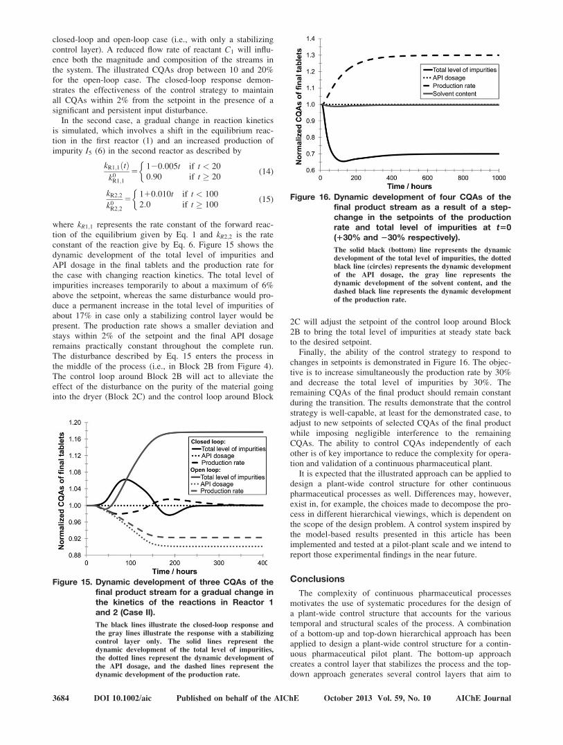
closed-loop and open-loop case (i.e., with only a stabilizingcontrol layer). A reduced flow rate of reactant C1 will influ-ence both the magnitude and composition of the streams inthe system. The illustrated CQAs drop between 10 and 20%for the open-loop case. The closed-loop response demon-strates the effectiveness of the control strategy to maintainall CQAs within 2% from the setpoint in the presence of asignificant and persistent input disturbance.

In the second case, a gradual change in reaction kineticsis simulated, which involves a shift in the equilibrium reac-tion in the first reactor (1) and an increased production ofimpurity I5 (6) in the second reactor as described by

kR1;1 tð Þk0

R1;1

5120:005t if t < 20

0:90 if t � 20

�(14)

kR2;2

k0R2;2

5110:010t if t < 100

2:0 if t � 100

�(15)

where kR1;1 represents the rate constant of the forward reac-tion of the equilibrium given by Eq. 1 and kR2;2 is the rateconstant of the reaction give by Eq. 6. Figure 15 shows thedynamic development of the total level of impurities andAPI dosage in the final tablets and the production rate forthe case with changing reaction kinetics. The total level ofimpurities increases temporarily to about a maximum of 6%above the setpoint, whereas the same disturbance would pro-duce a permanent increase in the total level of impurities ofabout 17% in case only a stabilizing control layer would bepresent. The production rate shows a smaller deviation andstays within 2% of the setpoint and the final API dosageremains practically constant throughout the complete run.The disturbance described by Eq. 15 enters the process inthe middle of the process (i.e., in Block 2B from Figure 4).The control loop around Block 2B will act to alleviate theeffect of the disturbance on the purity of the material goinginto the dryer (Block 2C) and the control loop around Block

2C will adjust the setpoint of the control loop around Block2B to bring the total level of impurities at steady state backto the desired setpoint.

Finally, the ability of the control strategy to respond tochanges in setpoints is demonstrated in Figure 16. The objec-tive is to increase simultaneously the production rate by 30%and decrease the total level of impurities by 30%. Theremaining CQAs of the final product should remain constantduring the transition. The results demonstrate that the controlstrategy is well-capable, at least for the demonstrated case, toadjust to new setpoints of selected CQAs of the final productwhile imposing negligible interference to the remainingCQAs. The ability to control CQAs independently of eachother is of key importance to reduce the complexity for opera-tion and validation of a continuous pharmaceutical plant.

It is expected that the illustrated approach can be applied todesign a plant-wide control structure for other continuouspharmaceutical processes as well. Differences may, however,exist in, for example, the choices made to decompose the pro-cess in different hierarchical viewings, which is dependent onthe scope of the design problem. A control system inspired bythe model-based results presented in this article has beenimplemented and tested at a pilot-plant scale and we intend toreport those experimental findings in the near future.

Conclusions

The complexity of continuous pharmaceutical processesmotivates the use of systematic procedures for the design ofa plant-wide control structure that accounts for the varioustemporal and structural scales of the process. A combinationof a bottom-up and top-down hierarchical approach has beenapplied to design a plant-wide control structure for a contin-uous pharmaceutical pilot plant. The bottom-up approachcreates a control layer that stabilizes the process and the top-down approach generates several control layers that aim to

Figure 16. Dynamic development of four CQAs of thefinal product stream as a result of a step-change in the setpoints of the productionrate and total level of impurities at t50(130% and 230% respectively).

The solid black (bottom) line represents the dynamic

development of the total level of impurities, the dotted

black line (circles) represents the dynamic development

of the API dosage, the gray line represents the

dynamic development of the solvent content, and the

dashed black line represents the dynamic development

of the production rate.

Figure 15. Dynamic development of three CQAs of thefinal product stream for a gradual change inthe kinetics of the reactions in Reactor 1and 2 (Case II).

The black lines illustrate the closed-loop response and

the gray lines illustrate the response with a stabilizing

control layer only. The solid lines represent the

dynamic development of the total level of impurities,

the dotted lines represent the dynamic development of

the API dosage, and the dashed lines represent the

dynamic development of the production rate.


maintain the CQAs of the final product close to a setpoint.The hierarchical nature of the control layers ensures that theeffect of a disturbance is mitigated at the relevant temporaland structural scale of the process. Sensitivity analysis canbe used to guide the selection of control loops at varioushierarchical levels for the presented case. Simulations of aplant-wide dynamic model including the control structureillustrate that the effect of significant and persistent distur-bances can be mitigated at each level of the hierarchicaldecomposition such that the overall effect of the disturbanceon the CQAs of the final product is significantly reduced.Furthermore, a case study illustrates that the system is well-capable to respond to a simultaneous change in the setpointof selected CQAs while the remaining CQAs are not affectedduring the transition period, which indicates flexibility tocontrol CQAs independently of each other.

Acknowledgments

The authors wish to acknowledge Novartis for support.The study presented in this article is inspired by a pilot plantthat has been constructed within the Novartis-MIT Centerfor Continuous Manufacturing. The authors wish to acknowl-edge the members of the team that have developed this pilotplant, in particular: Erin Bell, Stephen Born, Louis Buch-binder, Ellen Cappo, Josh Dittrich, James M. B. Evans, Pat-rick L. Heider, Devin R. Hersey, Rachael Hogan, AshleyKing, Tushar Kulkarni, Aaron Lamoureux, Salvatore Mascia,Sean Ogden, Joel Putnam, Justin Quon, Min Su, Kristen Tal-bot, Mengying Tao, Chris Testa, Forrest Whitcher, AaronWolfe, and Haitao Zhang.

Literature Cited

1. Kockmann N, Gottsponer M, Zimmermann B, Roberge DM. Ena-bling continuous-flow chemistry in microstructured devices for phar-maceutical and fine-chemical production. Chemistry. 2008;14:7470–7477.

2. Hartman RL, McMullen JP, Jensen KF. Deciding whether to go withthe flow: evaluating the merits of flow reactors for synthesis. AngewChem Int Ed. 2011;50:7502–7519.

3. Wegner J, Ceylan S, Kirschning A. Ten key issues in modern flowchemistry. Chem Commun. 2011;47:4583–4592.

4. Wegner J, Ceylan S, Kirschning A. Flow chemistry—a key enablingtechnology for (multistep) organic synthesis. Adv Synth Catal.2012;354:17–57.

5. Schaber SD, Gerogiorgis DI, Ramachandran R, Evans JMB, BartonPI, Trout BL. Economic analysis of integrated continuous and batchpharmaceutical manufacturing: a case study. Ind Eng Chem Res.2011;50:10083–10092.

6. Plumb K. Continuous processing in the pharmaceutical industry:changing the mind set. Chem Eng Res Des. 2005;83:730–738.

7. Roberge DM, Ducry L, Bieler N, Cretton P, Zimmermann B. Micro-reactor technology: a revolution for the fine chemical and pharma-ceutical industries? Chem Eng Technol. 2005;28:318–323.

8. Roberge DM, Zimmermann B, Rainone F, Gottsponer M, EyholzerM, Kockmann N. Microreactor technology and continuous processesin the fine chemical and pharmaceutical industry: is the revolutionunderway? Org Process Res Dev. 2008;12:905–910.

9. Jimenez-Gonzalez C, Poechlauer P, Broxterman QB, Yang BS, amEnde D, Baird J, Bertsch C, Hannah RE, Dell’Orco P, Noorrnan H,Yee S, Reintjens R, Wells A, Massonneau V, Manley J. Key greenengineering research areas for sustainable manufacturing: a perspec-tive from pharmaceutical and fine chemicals manufacturers. OrgProcess Res Dev. 2011;15:900–911.

10. LaPorte TL, Wang C. Continuous processes for the production ofpharmaceutical intermediates and active pharmaceutical ingredients.Curr Opin Drug Discov Devel. 2007;10:738–745.

11. Pollet P, Cope ED, Kassner MK, Charney R, Terett SH, RichmanKW, Dubay W, Stringer J, Eckertt CA, Liotta CL. Production of

(S)-1-benzyl-3-diazo-2-oxopropylcarbamic acid tert-butyl ester, adiazoketone pharmaceutical intermediate, employing a small scalecontinuous reactor. Ind Eng Chem Res. 2009;48:7032–7036.

12. Christensen KM, Pedersen MJ, Dam-Johansen K, Holm TL, SkovbyT, Kiil S. Design and operation of a filter reactor for continuous pro-duction of a selected pharmaceutical intermediate. Chem Eng Sci.2012;26:111–117.

13. Cervera-Padrell AE, Skovby T, Kiil S, Gani R, Gernaey KV. Activepharmaceutical ingredient (API) production involving continuousprocesses—a process systems engineering (PSE)-assisted designframework. Eur J Pharm Biopharm. 2012;82:437–456.

14. Buckley PS. Techniques of Process Control. New York: John Wileyand Sons, 1964.

15. Morari M, Arkun Y, Stephanopoulos G. Studies in the synthesis ofcontrol structures for chemical processes: part 1. Formulation of theproblem. Process decomposition and the classification of the controltasks. Analysis of the optimizing control structures. AIChE J.1980;26:220–232.

16. Morari M, Stephanopoulos G. Studies in the synthesis of controlstructures for chemical processes: part II. Structural aspects and thesynthesis of alternative feasible control schemes. AIChE J.1980;26:232–246.

17. Larsson T, Skogestad S. Plantwide control—a review and a newdesign procedure. Int J Model Identif Control. 2000;21:209–240.

18. Stephanopoulos G, Ng C. Perspectives on the synthesis of plant-wide control structures. J Process Control. 2000;10:97–111.

19. Douglas JM. A hierarchical decision procedure for process synthesis.AIChE J. 1985;31:353–362.

20. Baldea M, Daoutidis P. Control of integrated process networks—amultitime scale perspective. Comput Chem Eng. 2007;31:426–444.

21. Yu LX. Pharmaceutical quality by design: product and process devel-opment, understanding, and control. Pharm Res. 2008;25:781–791.

22. ICH. Guidance for Industry Q8(R2) Pharmaceutical Development.Silver Spring, MD, 2009, http://www.fda.gov/downloads/Drugs/ Gui-danceComplianceRegulatoryInformation/Guidances/ucm073507.pdf.

23. Lionberger RA, Lee SL, Lee L, Raw A, Yu LX. Quality by design:concepts for ANDAs. AAPS J. 2008;10:268–276.

24. Singh R, Ierapetritou M, Ramachandran R. An engineering study onthe enhanced control and operation of continuous manufacturing ofpharmaceutical tablets via roller compaction. Int J Pharm.2012;438:307–326.

25. Gernaey KV, Gani R. A model-based systems approach to pharma-ceutical product-process design and analysis. Chem Eng Sci.2010;65:5757–5769.

26. Gernaey KV, Cervera-Padrell AE, Woodley JM. Development ofcontinuous pharmaceutical production processes supported by pro-cess systems engineering methods and tools. Future Med Chem.2012;4:1371–1374.

27. Boukouvala F, Niotis V, Ramachandran R, Muzzio FJ, Ierapetritou

MG. An integrated approach for dynamic flowsheet modeling and

sensitivity analysis of a continuous tablet manufacturing process.

Comput Chem Eng. 2012;42:30–47.28. Benyahia B, Lakerveld R, Barton PI. A plant-wide dynamic model

of a continuous pharmaceutical process. Ind Eng Chem Res.2012;51:15393–15412.

29. Skogestad S. Control structure design for complete chemical plants.Comput Chem Eng. 2004;28:219–234.

30. Ng CS, Stephanopoulos G. Synthesis of control systems for chemicalplants. Comput Chem Eng. 1996;20:S999–S1004.

31. Singh R, Gernaey KV, Gani R. Model-based computer-aided frame-work for design of process monitoring and analysis systems. ComputChem Eng. 2009;33:22–42.

32. Feehery WF, Tolsma JE, Barton PI. Efficient sensitivity analysis oflarge-scale differential-algebraic systems. Appl Numer Math.1997;25:41–54.

33. Galan S, Feehery WF, Barton PI. Parametric sensitivity functions forhybrid discrete/continuous systems. Appl Numer Math. 1999;31:17–47.

34. Luyben WL. Snowball effects in reactor/separator processes withrecycle. Ind Eng Chem Res. 1994;33:299–305.

35. McDonald KA, McAvoy TJ, Tits A. Optimal averaging level con-trol. AIChE J. 1986;32:75–86.

36. Seborg DE, Edgar TF, Mellichamp DA. Process Dynamics and Con-trol. New York: John Wiley and Sons, 1989.

Manuscript received Nov. 23, 2012, and revision received Feb. 26, 2013.


Documents

Model-Based Design of a Plant-Wide Control Strategy …web.mit.edu/.../model_based_design_of_a_plantwide_control_strategy...Model-Based Design of a Plant-Wide Control Strategy for