MODAEM - Aquaveo

Page 1 of 13 © Aquaveo

GMS TUTORIALS

MODAEM

MODAEM is a single-layer, steady-state analytic element groundwater flow model that

has been enhanced for use with GMS. This chapter introduces MODAEM to the new

user and illustrates the use of GMS for analytic element modeling. This tutorial does not

go into detail in explaining the analytic element method. For a more detailed explanation

of analytic element modeling and MODAEM, refer to the GMS Help.

You should have completed the GMS Basics tutorial prior to completing this one, and

should be familiar with Feature Objects.

1.1 Outline

This is what you will do:

1. Read in a background map.

2. Create a conceptual model and define the parameters.

3. Run MODAEM for different conditions.

1.2 Required Modules/Interfaces

You will need the following components enabled to complete this tutorial:

• Map

• MODAEM

You can see if these components are enabled by selecting the File | Register command.

GMS Tutorials MODAEM


2 Description of Problem

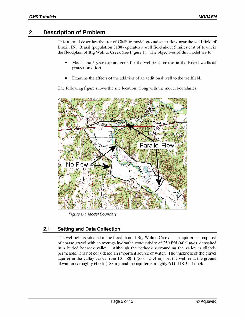
This tutorial describes the use of GMS to model groundwater flow near the well field of

Brazil, IN. Brazil (population 8188) operates a well field about 5 miles east of town, in

the floodplain of Big Walnut Creek (see Figure 1). The objectives of this model are to:

• Model the 5-year capture zone for the wellfield for use in the Brazil wellhead

protection effort.

• Examine the effects of the addition of an additional well to the wellfield.

The following figure shows the site location, along with the model boundaries.

Figure 2-1 Model Boundary

2.1 Setting and Data Collection

The wellfield is situated in the floodplain of Big Walnut Creek. The aquifer is composed

of coarse gravel with an average hydraulic conductivity of 250 ft/d (60.9 m/d), deposited

in a buried bedrock valley. Although the bedrock surrounding the valley is slightly

permeable, it is not considered an important source of water. The thickness of the gravel

aquifer in the valley varies from 10 – 80 ft (3.0 – 24.4 m). At the wellfield, the ground

elevation is roughly 600 ft (183 m), and the aquifer is roughly 60 ft (18.3 m) thick.



3 Getting Started

Let’s get started.

1. If necessary, launch GMS. If GMS is already running, select the File | New

command to ensure that the program settings are restored to their default state.

4 Reading in the Background Map

The first step to create our model is to read in a background image of the site we are

modeling. We will use the image to guide us as we create points, arcs, and polygons to

define features of our model.

1. Select the Open button .

2. Locate and open the directory entitled tutfiles\MODAEM\modaem.

3. Change the Files of type to Images (*.tif; *.tiff; *.jpg; *.jpeg; *.png; *.sid).

4. Select and open the file indiana.jpg.

5. Select Yes if prompted to generate image pyramids.

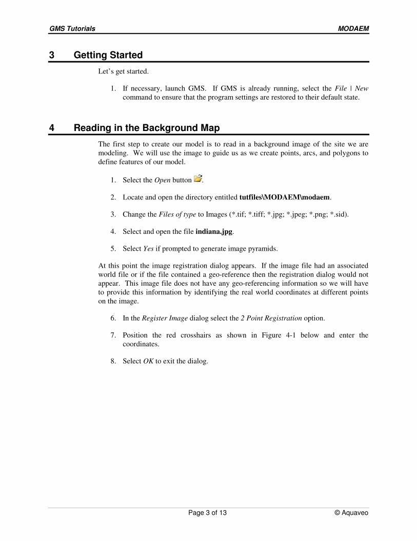
At this point the image registration dialog appears. If the image file had an associated

world file or if the file contained a geo-reference then the registration dialog would not

appear. This image file does not have any geo-referencing information so we will have

to provide this information by identifying the real world coordinates at different points

on the image.

6. In the Register Image dialog select the 2 Point Registration option.

7. Position the red crosshairs as shown in Figure 4-1 below and enter the

coordinates.

8. Select OK to exit the dialog.



Figure 4-1 Image Registration

5 Defining the Units

At this point, we can also define the units used in the conceptual model. The units we

choose will be applied to edit fields in the GMS interface to remind us of the proper units

for each parameter.

1. Select the Edit | Units command.

2. For Length, select m (for meters). For Time, select d (for days). We will ignore

the other units (they are not used for flow simulations).

3. Select the OK button.

6 Creating the Conceptual Model

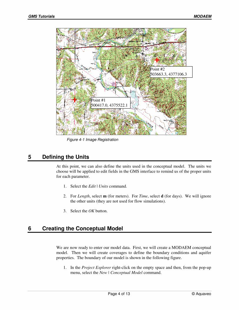
We are now ready to enter our model data. First, we will create a MODAEM conceptual

model. Then we will create coverages to define the boundary conditions and aquifer

properties. The boundary of our model is shown in the following figure.

1. In the Project Explorer right-click on the empty space and then, from the pop-up

menu, select the New | Conceptual Model command.

Point #1

500417.0, 4375522.1

Point #2

503663.3, 4377106.3



2. Change the Name to Indiana and the Type to MODAEM and click OK.

3. Right click on the Indiana conceptual model and select the New Coverage

menu command.

4. Change the Coverage name to Boundary and select the Use to define model

boundary option. Click OK.

5. Select the Zoom tool .

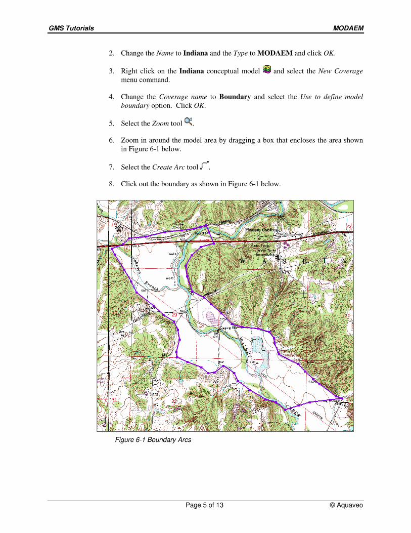
6. Zoom in around the model area by dragging a box that encloses the area shown

in Figure 6-1 below.

7. Select the Create Arc tool .

8. Click out the boundary as shown in Figure 6-1 below.

Figure 6-1 Boundary Arcs



7 Creating the Specified Head Arcs

By default, the arcs in a MODAEM boundary coverage are “no flow” boundaries. This

means the arcs’ type is set to “specified flow” and the flow is set to 0. Next we will add

specified head arcs to this coverage. To create the specified head arcs we will split the

boundary arc into four separate arcs.

7.1 Convert Vertices to Nodes

1. Select the Select Objects tool .

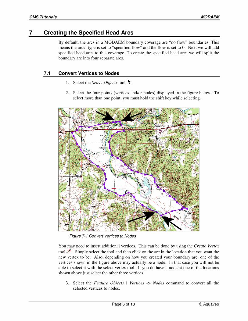
2. Select the four points (vertices and/or nodes) displayed in the figure below. To

select more than one point, you must hold the shift key while selecting.

Figure 7-1 Convert Vertices to Nodes

You may need to insert additional vertices. This can be done by using the Create Vertex

tool . Simply select the tool and then click on the arc in the location that you want the

new vertex to be. Also, depending on how you created your boundary arc, one of the

vertices shown in the figure above may actually be a node. In that case you will not be

able to select it with the select vertex tool. If you do have a node at one of the locations

shown above just select the other three vertices.

3. Select the Feature Objects | Vertices -> Nodes command to convert all the

selected vertices to nodes.



7.2 Assigning Arcs

1. Select the Select Arcs tool .

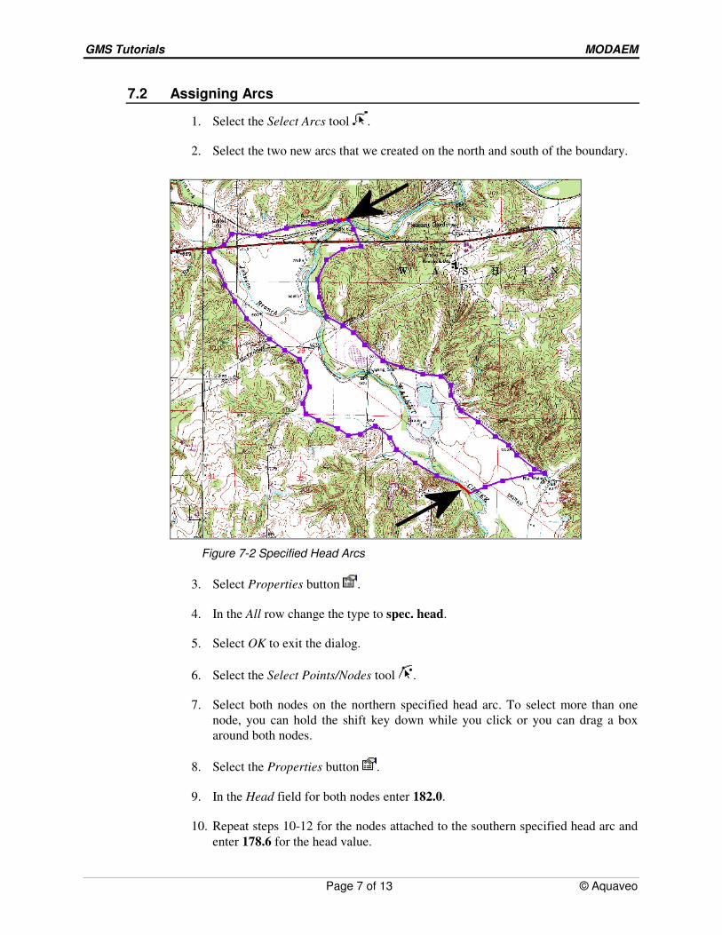
2. Select the two new arcs that we created on the north and south of the boundary.

Figure 7-2 Specified Head Arcs

3. Select Properties button .

4. In the All row change the type to spec. head.


6. Select the Select Points/Nodes tool .

7. Select both nodes on the northern specified head arc. To select more than one

node, you can hold the shift key down while you click or you can drag a box

around both nodes.

8. Select the Properties button .

9. In the Head field for both nodes enter 182.0.

10. Repeat steps 10-12 for the nodes attached to the southern specified head arc and

enter 178.6 for the head value.



8 Entering the Aquifer Properties

Next we will enter the properties of our aquifer. Aquifer properties can be assigned to

individual polygons, and we can also define properties for a “background aquifer.”

1. Select the MODAEM | Global Options command.

2. In the Background aquifer properties section enter 170.0 for the Base, 18.0 for

the Thickness, and 60.0 for the Hyd. cond.


With a boundary coverage we must also have a single polygon that defines the aquifer

we are modeling.

4. Select the Feature Objects | Build Polygons command.

9 Saving the Project

We are now ready to run MODAEM. With other models in GMS, like MODFLOW for

example, you must first save your changes to the project before you run the model.

When you run MODAEM, however, the data currently in memory is written to

temporary files that MODAEM reads to compute its solution. Therefore, you don’t have

to save your changes in GMS before running MODAEM. However, it’s a good idea to

save your work periodically anyway, so let’s do so now.

1. Select the File | Save As command.

2. Save the project with the name brazil.

Now you can hit the save button periodically as you develop your model.

10 Running MODAEM

We are now ready to run MODAEM. This can be done by selecting the menu command

MODAEM | Solve or by hitting the F5 key. Once this command is executed a dialog will

appear showing the output from the MODAEM model.

1. Hit the F5 key.

2. When MODAEM is finished, select the Close button.

Head contours should now appear inside our boundary coverage.

3. Select the Display Options button .

4. Select the MODAEM tab.



5. Click on the Options button next to the Contours toggle.

6. Change the Contour method to Linear and Color Fill.

7. Under the Fill options section of the dialog change the Transparency value to

0.4.

8. Under the Fill options section select the Color Ramp button.

9. Under the Palette Method section of the dialog, turn on Legend.

10. Select OK repeatedly to close all of the dialogs.

11 Creating the River

Now we will add the river to our model.

1. Right click on Indiana in the Project Explorer and select the New Coverage

option.

2. Change the name of the coverage to River.

3. Under the Source/Sink/BCs section toggle on the River option.


5. Select the Create Arc tool .

6. Click out the river arc starting near the northern specified head boundary and

ending near the southern specified head boundary, as shown in Figure 11-1

below. Don’t extend the river beyond the boundary coverage.



Figure 11-1 Modeling the River

7. Select the Select Arcs tool .

8. Click anywhere on the river arc to select it.

9. Select Properties button .

10. Change the type of the arc to river.

11. Enter a value of 5000.0 for the Cond. (conductance) and click OK.

12. Select the Select Points/Nodes tool .

13. Double click on the river node at the northern end of the model.

14. Enter 182.0 for the Head and 179.0 for the Elev.


16. Repeat the same process for the southern river node and enter 178.6 for the Head

and 175.6 for the Elev.

12 Running MODAEM

We are now ready to run MODAEM again.

1. Hit the F5 key.




You should notice some change in the head contours, particularly around the river arc.

13 Adding Recharge

Now we will add recharge to the model.

1. Right-click on the Boundary coverage and select the Duplicate command.

2. Double click on the Copy of Boundary coverage.

3. Change the name to Recharge.

4. In the Sources/Sinks/BCs section of the dialog, toggle off Specified Head and

Specified Flow.

5. In the Areal Properties section of the dialog, toggle on Recharge.


7. Select the Select Polygons tool .

8. Double click on the polygon and assign a value of .000420 to the Recharge field.

Click OK to exit the dialog.

14 Running MODAEM


1. Hit the F5 key.


15 Production Wells

Now we will import production wells from a tab delimited text file.

1. Right-click on Indiana in the Project Explorer and select the New Coverage

option.

2. Change the name of the coverage to Wells.

3. Under the Source/Sink/BCs section toggle on the Wells option.





6. Locate and open the directory entitled tutfiles\modaem.

7. Select and open the file prod_wells.txt.

8. Toggle on the Heading row toggle.

9. Click the Next > button.

10. Change the GMS data type to Well data.

11. In the File preview section of the dialog change the Type of the first column to

X, the second to Y, and the third to Flow Rate.

12. Select the Finish button to exit the dialog.

You may have difficulty seeing the wells. The well symbol can be changed in the

Display Options dialog by clicking on the Display macro .

16 Observation Wells

Before running MODAEM again we will also read in field measured head values.

1. Right-click on Indiana in the Project Explorer and select the New Coverage

option.

2. Change the name of the coverage to Observation.

3. Under the Observation Points section toggle on the Head option.



6. Locate and open the directory entitled tutfiles\modaem.

7. Select and open the file well_head.txt.

8. Toggle on the Heading row toggle.

9. Click the Next > button.

10. Change the GMS data type to Observation data.

11. In the File preview section of the dialog change the Type of the first column to

Name, the second to X, the third to Y, and the fourth to Obs. Head.

12. Select the Finish button to exit the dialog.



13. You should now see observation targets appear.

17 Running MODAEM


1. Hit the F5 key.


18 Conclusion

This concludes the tutorial. Here are the things that you should have learned in this

tutorial:

• MODAEM is an analytic element model located in the Map module of GMS,

and it uses points, arcs, and polygons to compute solutions.

• Images that do not come with registration information can be registered in GMS

so that they are displayed in the appropriate location in your model coordinate

system.

• The Map module is used to construct conceptual models using feature objects

(points, arcs and polygons).

• Feature objects are grouped into coverages. There is always only one active

coverage, and only the active coverage can be edited.

Documents

MODAEM - Aquaveo