Groundwater Analyst - Wells and Time Series - Aquaveo

Page 1 of 26 © Aquaveo

ARC HYDRO GROUNDWATER TUTORIALS

Wells and Time Series

Arc Hydro Groundwater (AHGW) is a geodatabase design for representing groundwater

datasets within ArcGIS. The data model helps to archive, display, and analyze

multidimensional groundwater data, and includes several components to represent different

types of datasets, including representations of aquifers and wells/boreholes, 3D

hydrogeologic models, temporal information, and data from simulation models.

The Arc Hydro Groundwater Tools help to import, edit, and manage groundwater data

stored in an AHGW geodatabase. This tutorial illustrates how to use the tools to manage

well data and time series data (transient water level measurements) associated with wells.

A basic familiarity with the AHGW data model is suggested, but not required, prior to

beginning this tutorial.

1.1 Outline

In this tutorial, we will be working with groundwater data from the Panhandle region of

Texas. We will complete the following tasks:

1. Import a set of well data into ArcGIS.

2. Modify the well attributes.

3. Generate time series plots of water level data.

4. Generate average water level maps for selected periods.

5. Build a geoprocessing model to automate running a tool.

6. Generate a flow direction map.

Arc Hydro GW Tutorials Wells and Time Series


1.2 Required Modules/Interfaces

You will need the following components enabled in order to complete this tutorial:

Arc View license (or ArcEditor\ArcInfo)

Arc Hydro Groundwater Tools

Spatial Analyst or 3D Analyst extension

AHGW Tutorial Files

The AHGW Tools requires that you have a compatible ArcGIS service pack installed. You

may wish to check the AHGW Tools documentation to find the appropriate service pack

for your version of the tools. Spatial Analyst is required for one portion of the tutorial

involving interpolation. If you do not have Spatial Analyst, you can skip that portion of the

tutorial. The tutorial files should be downloaded to your computer and saved on a local

drive.

2 Getting Started

Before opening our map, let’s ensure that the AHGW Tools are correctly configured.

1. If necessary, launch ArcMap.

2. If necessary, open the ArcToolbox window by clicking on the ArcToolbox icon

.

3. Make sure the Arc Hydro Groundwater Toolboxes is loaded. If it is not, add the

toolboxe by right-clicking anywhere in the ArcToolbox window and selecting the

Add Toolbox… command. Browse to the top level of the Catalog and then browse

down to the Toolboxes|System Toolboxes directory. Select the toolbox and select

the Open button.

4. Expand the Arc Hydro Groundwater Tools item and then expand the

Groundwater Analyst toolset to expose the tools we will be using in this tutorial.

Note that many of the GP tools in the AHGW Toolbox can also be accessed from the

AHGW Toolbar. The toolbar contains additional user interface components not available

in the toolbox. If the toolbar is not visible, do the following:

5. Right-click on any visible toolbar and select the Arc Hydro Groundwater Toolbar

item.

When using geoprocessing tools you can set the tools to overwrite outputs by default, and

automatically add results to the map/scene. To set these options:

6. Open ArcMap/ArcCatalog (if not already open).



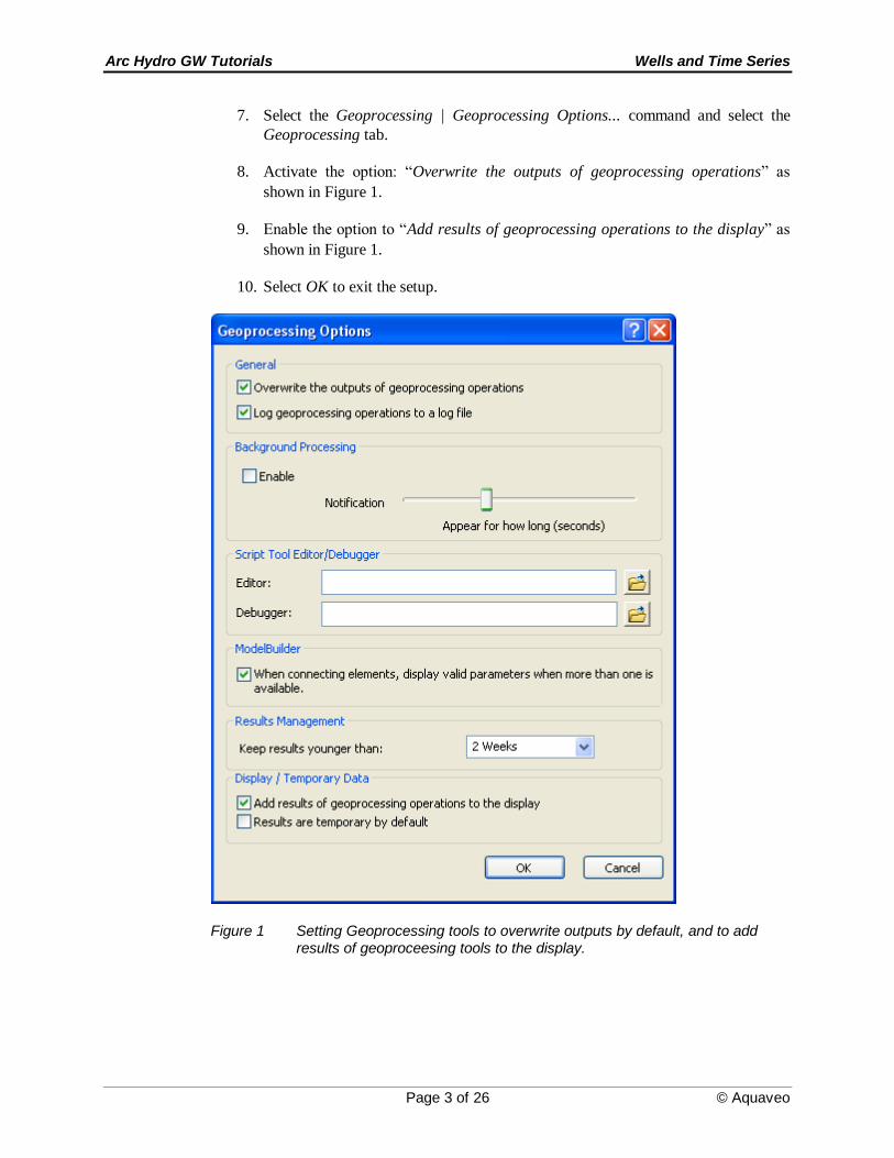
7. Select the Geoprocessing | Geoprocessing Options... command and select the

Geoprocessing tab.

8. Activate the option: “Overwrite the outputs of geoprocessing operations” as

shown in ‎Figure 1.

9. Enable the option to “Add results of geoprocessing operations to the display” as


10. Select OK to exit the setup.

Figure 1 Setting Geoprocessing tools to overwrite outputs by default, and to add results of geoproceesing tools to the display.



3 Opening the Map

We will begin by opening a map containing county boundaries for the Panhandle region of

North Texas.

1. Select the File | Open command and browse to the location on your local drive

where you have saved the AHGW tutorials. Browse to the Groundwater Analyst |

wells and time series folder and open the file entitled lubbock_wells.mxd.

Once the file has loaded you will see a map of the Panhandle region of North Texas. The

filled polygon represents the boundary of the Ogallala aquifer in Texas. This data was

obtained from the Texas Water Development Board Groundwater Database

(http://www.twdb.state.tx.us/publications/reports/groundwaterreports/gwdatabasereports/g

wdatabaserpt.htm).

4 Importing the Well Data

Next, we will import the well data for Lubbock County. The well data has been

downloaded from the above-referenced website to a comma-delimited text file. The AHGW

Tools include a tool for automating the import of text data into a AHGW geodatabase.

1. In the AHGW Toolbar, select the Arc Hydro GW | Text Import command.

2. In the wells and time series folder, select and open the lubbock_well_data.txt

file.

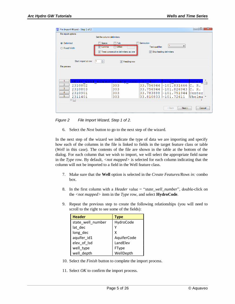
3. At the top of the File Import Wizard, turn on the Comma toggle and turn off the

Space toggle in the column delimiters section.

4. Turn on the Treat consecutive delimiters as one toggle.

5. Turn on the Heading row toggle. This indicates that the first row contains headers

for the data.

At this point, the dialog should look like the example shown in ‎Figure 2.



Figure 2 File Import Wizard, Step 1 of 2.

6. Select the Next button to go to the next step of the wizard.

In the next step of the wizard we indicate the type of data we are importing and specify

how each of the columns in the file is linked to fields in the target feature class or table

(Well in this case). The contents of the file are shown in the table at the bottom of the

dialog. For each column that we wish to import, we will select the appropriate field name

in the Type row. By default, <not mapped> is selected for each column indicating that the

column will not be imported to a field in the Well feature class.

7. Make sure that the Well option is selected in the Create Features/Rows in: combo

box.

8. In the first column with a Header value = “state_well_number”, double-click on

the <not mapped> item in the Type row, and select HydroCode.

9. Repeat the previous step to create the following relationships (you will need to

scroll to the right to see some of the fields):

Header Type

state_well_number lat_dec

HydroCode Y

long_dec X aquifer_id1 AquiferCode elev_of_lsd LandElev well_type FType well_depth WellDepth

10. Select the Finish button to complete the import process.

11. Select OK to confirm the import process.



At this point, you should see wells appear in the map.

Before continuing, let’s zoom in on the wells.

12. Select the Zoom In tool and drag a box around the wells.

5 Using the Feature Type Filter

Features such as wells include an FType field representing the feature type. For wells, this

field is often populated with values such as “irrigation”, “municipal”, etc. The AHGW

Toolbar includes a pair of filters that can be used to map only the features in a layer that

correspond to a particular type. The Filter creates a simple definition query for the selected

value (for example, FType = ‘irrigation’). The Texas Water Development Board uses

single character codes to identify well types. The four codes used in the wells in Lubbock

County are O, S, T, and W and represent the following well types:

Code Well Type

O Observation S Spring T Test hole W Withdrawal

Before using the filter, we will first change the symbology so that the wells are colored by

type.

1. In the Table of Contents, right-click on the Well layer and select the Properties

command.

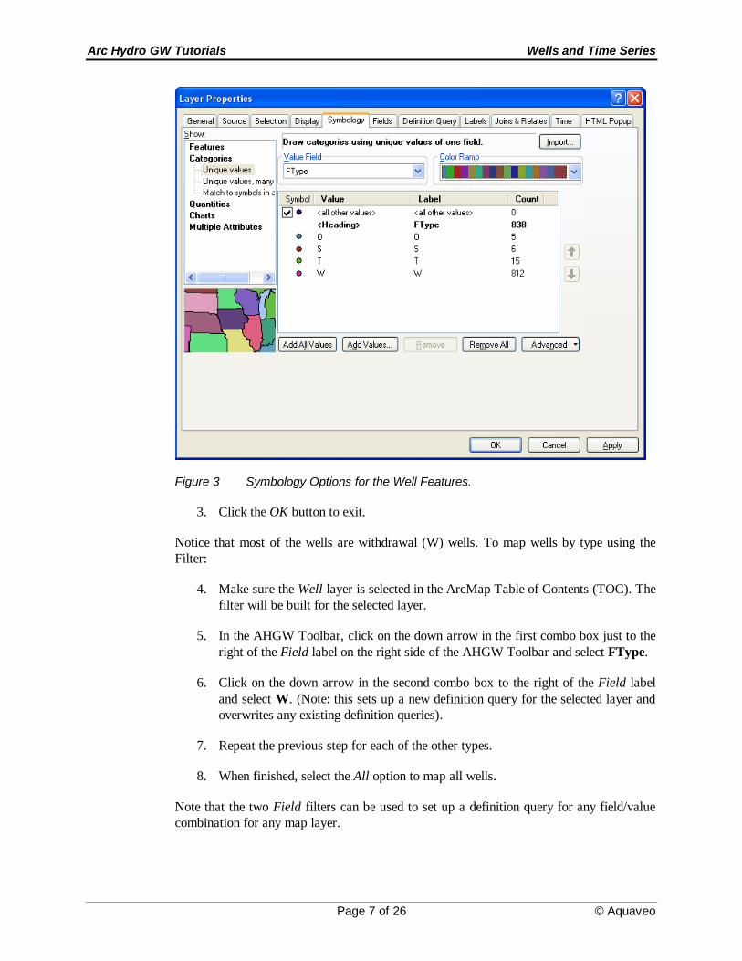
2. Click on the Symbology tab in the Layer Properties dialog, and change the

selected options to match those shown in ‎Figure 3 (Change the Show: option to

Categories | Unique values. Choose FType as the value field and click the Add

All Values button.).



Figure 3 Symbology Options for the Well Features.

3. Click the OK button to exit.

Notice that most of the wells are withdrawal (W) wells. To map wells by type using the

Filter:

4. Make sure the Well layer is selected in the ArcMap Table of Contents (TOC). The

filter will be built for the selected layer.

5. In the AHGW Toolbar, click on the down arrow in the first combo box just to the

right of the Field label on the right side of the AHGW Toolbar and select FType.

6. Click on the down arrow in the second combo box to the right of the Field label

and select W. (Note: this sets up a new definition query for the selected layer and

overwrites any existing definition queries).

7. Repeat the previous step for each of the other types.

8. When finished, select the All option to map all wells.

Note that the two Field filters can be used to set up a definition query for any field/value

combination for any map layer.



6 Assigning HydroIDs

Each feature in an Arc Hydro geodatabase should have an identifier that is unique across

the entire geodatabase, not just within a feature class. This unique ID is called the

HydroID. The HydroID is used to build relationships between feature classes and/or

tables. For example, we will use the HydroIDs of the wells to relate the wells to the

corresponding water level measurements in the TimeSeries table.

In a typical project, one would normally use the Assign HydroID GW tool in the

Groundwater Analyst toolset to generate unique HydroIDs for new features. This tool

necessitates some additional steps to relate the wells to the time series data we will import

in the next step. Therefore, in order to keep this tutorial simple we will copy over the

values in the HydroCode field to the HydroID field. This will result in unique integer IDs

for this exercise. To copy the values:

1. Right-click on the Well layer in the ArcMap Table of Contents window and select

Open Attribute Table.

2. Right-click on the HydroID field and select the Field Calculator command. Click

Yes if necessary at the warning about an edit session.

3. In the Fields section of the Field Calculator, double-click on the HydroCode item.

4. Select the OK button.

You should see that the values in the HydroID field match the values in the HydroCode

field.

5. Close the Attributes window.

7 Importing the Time Series Data

Now that we have imported the well features, we are ready to import transient water level

measurements into the TimeSeries table. Each record in the table will represent a water

level measurement at a particular well at a particular time. The records in the TimeSeries

table will be related to the wells using the HydroID field.

Once again, we will use the Text Import Wizard to import the data.

1. In the AHGW Toolbar, select the Arc Hydro GW | Text Import command.

2. In the wells and time series folder, select and open the lubbock_water_levels.txt

file.

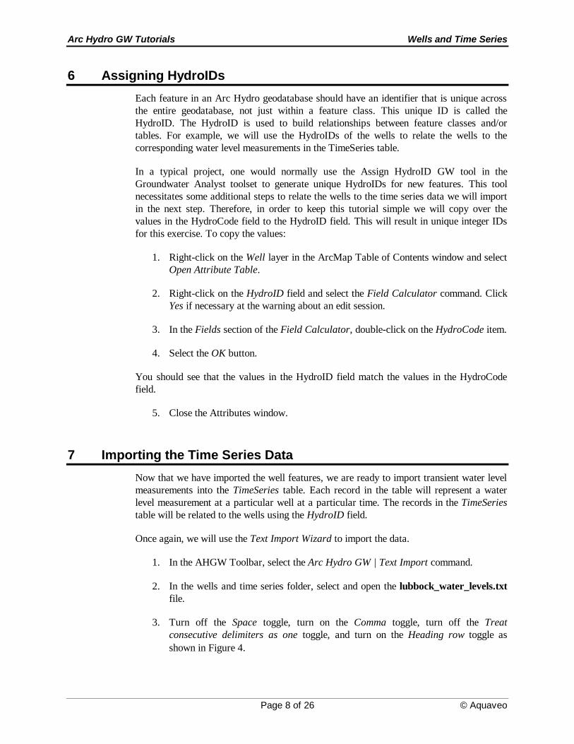
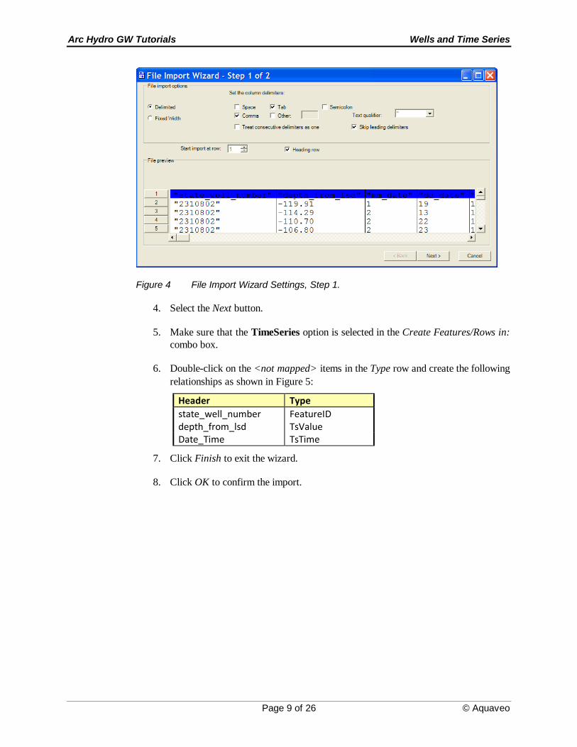
3. Turn off the Space toggle, turn on the Comma toggle, turn off the Treat

consecutive delimiters as one toggle, and turn on the Heading row toggle as




Figure 4 File Import Wizard Settings, Step 1.

4. Select the Next button.

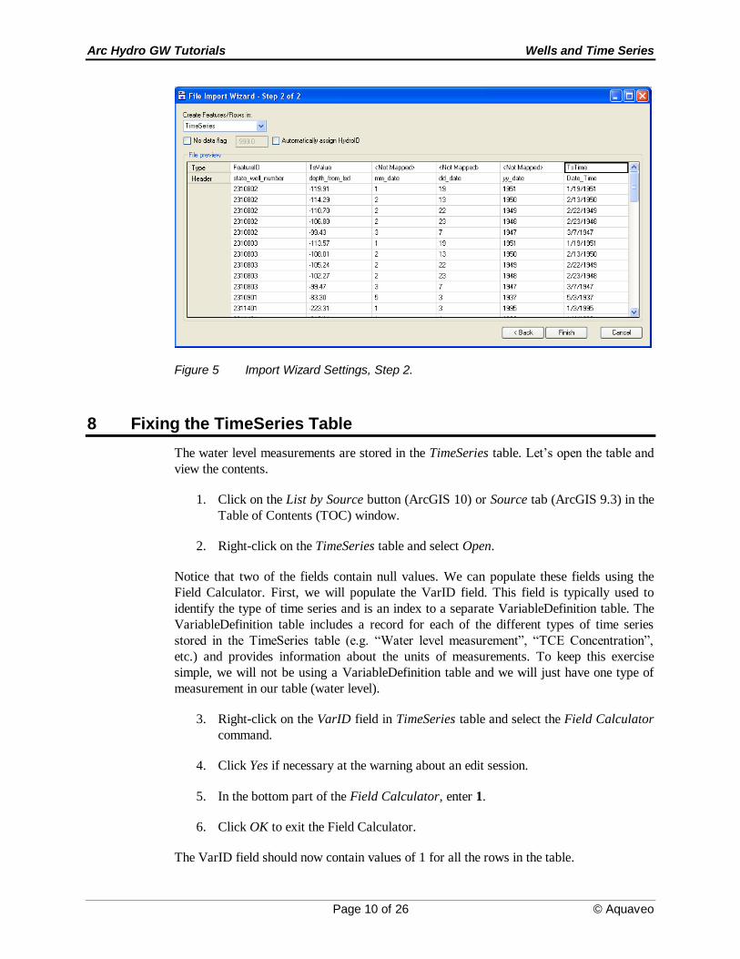
5. Make sure that the TimeSeries option is selected in the Create Features/Rows in:

combo box.

6. Double-click on the <not mapped> items in the Type row and create the following

relationships as shown in ‎Figure 5:

Header Type

state_well_number FeatureID depth_from_lsd TsValue Date_Time TsTime

7. Click Finish to exit the wizard.

8. Click OK to confirm the import.



Figure 5 Import Wizard Settings, Step 2.

8 Fixing the TimeSeries Table

The water level measurements are stored in the TimeSeries table. Let’s open the table and

view the contents.

1. Click on the List by Source button (ArcGIS 10) or Source tab (ArcGIS 9.3) in the

Table of Contents (TOC) window.

2. Right-click on the TimeSeries table and select Open.

Notice that two of the fields contain null values. We can populate these fields using the

Field Calculator. First, we will populate the VarID field. This field is typically used to

identify the type of time series and is an index to a separate VariableDefinition table. The

VariableDefinition table includes a record for each of the different types of time series

stored in the TimeSeries table (e.g. “Water level measurement”, “TCE Concentration”,

etc.) and provides information about the units of measurements. To keep this exercise

simple, we will not be using a VariableDefinition table and we will just have one type of

measurement in our table (water level).

3. Right-click on the VarID field in TimeSeries table and select the Field Calculator

command.

4. Click Yes if necessary at the warning about an edit session.

5. In the bottom part of the Field Calculator, enter 1.

6. Click OK to exit the Field Calculator.

The VarID field should now contain values of 1 for all the rows in the table.



Next, we will make an adjustment to the water level measurements in the TimeSeries table.

The water levels we imported to the TsValue field are actually depths measured from the

top of the well and are expressed as negative values. To get a field representing actual

elevations, we will use the field calculator and add the negative depths to the well

elevations. This will require a temporary join. We will put the adjusted elevation values

into a field called TSValue_normalized.

First, we will do the join.

7. Close the TimeSeries table.

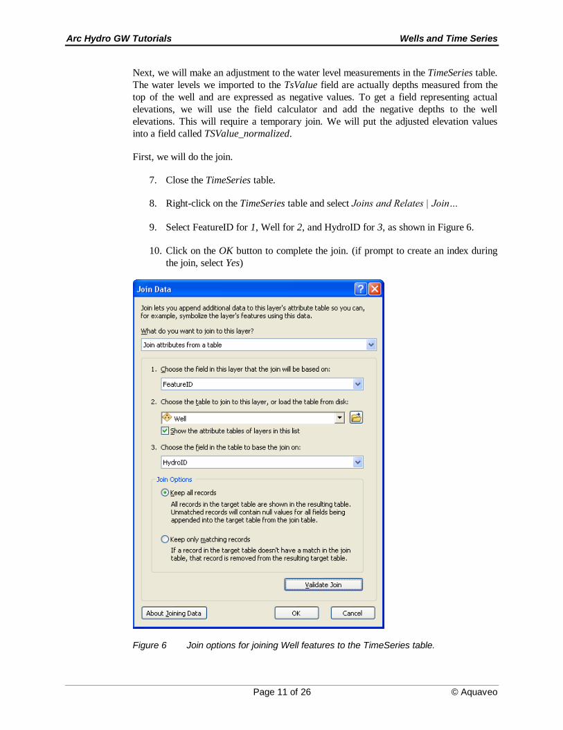
8. Right-click on the TimeSeries table and select Joins and Relates | Join…

9. Select FeatureID for 1, Well for 2, and HydroID for 3, as shown in ‎Figure 6.

10. Click on the OK button to complete the join. (if prompt to create an index during

the join, select Yes)

Figure 6 Join options for joining Well features to the TimeSeries table.



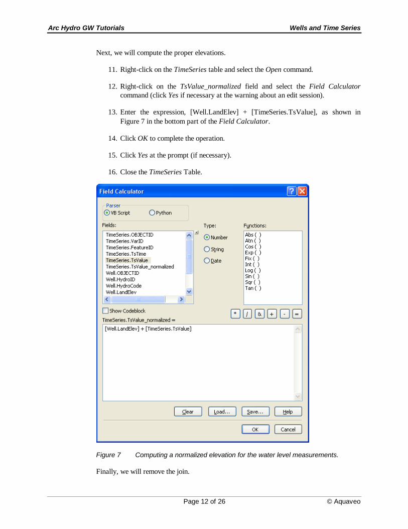
Next, we will compute the proper elevations.

11. Right-click on the TimeSeries table and select the Open command.

12. Right-click on the TsValue_normalized field and select the Field Calculator

command (click Yes if necessary at the warning about an edit session).

13. Enter the expression, [Well.LandElev] + [TimeSeries.TsValue], as shown in

‎Figure 7 in the bottom part of the Field Calculator.

14. Click OK to complete the operation.

15. Click Yes at the prompt (if necessary).

16. Close the TimeSeries Table.

Figure 7 Computing a normalized elevation for the water level measurements.

Finally, we will remove the join.



17. Right-click on the TimeSeries table and select Joins and Relates | Remove Join(s)

| Well.

9 Finding Wells with Transient Data

Some of the wells imported have transient water level measurements and some do not. We

can quickly determine which wells have transient data using the Make Time Series

Statistics tool in the Groundwater Analyst toolset. This tool can be used to derive a new

feature set from an existing feature set with transient data. The new feature set includes a

field representing selected statistics of the original transient data (mean, standard

deviation, etc.). In this case, we will use the tool to derive a new layer containing only the

wells with transient data and with a field representing the average water level over all

measurements.

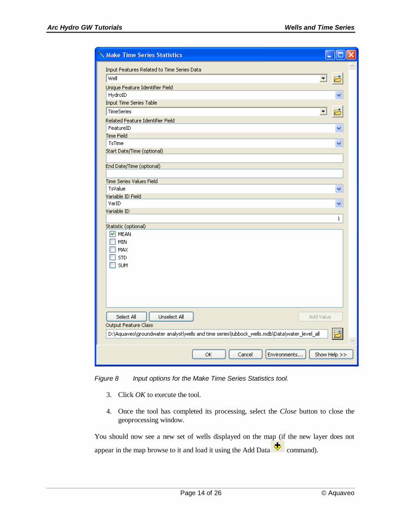
1. Double-click on the Make Time Series Statistics tool in the AHGW Toolbox |

Groundwater Analyst toolset.

2. Enter the input options/selections as shown in ‎Figure 8. For the Output Feature

Class option, browse to the location on your local drive where the tutorial files are

located and open the Lubbock_wells geodatabase so that the new features are

created inside the geodatabase. Type water_level_all as the name of your new

feature class.



Figure 8 Input options for the Make Time Series Statistics tool.

3. Click OK to execute the tool.

4. Once the tool has completed its processing, select the Close button to close the

geoprocessing window.

You should now see a new set of wells displayed on the map (if the new layer does not

appear in the map browse to it and load it using the Add Data command).



10 Adjusting the Well Display

In addition to the mean water level, the Make Time Series Statistics tool generates a new

field containing the frequency of measurements (i.e., the number of transient water level

values per well). We can use ArcMap Symbology to map the sampling frequency.

1. Uncheck the Well layer to hide that layer. Only wells with transient data will still

be visible in the map.

2. Right-click on the water_level_all layer and select the Properties command.

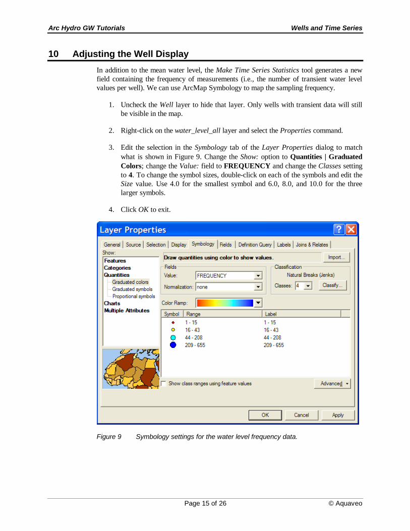
3. Edit the selection in the Symbology tab of the Layer Properties dialog to match

what is shown in ‎Figure 9. Change the Show: option to Quantities | Graduated

Colors; change the Value: field to FREQUENCY and change the Classes setting

to 4. To change the symbol sizes, double-click on each of the symbols and edit the

Size value. Use 4.0 for the smallest symbol and 6.0, 8.0, and 10.0 for the three

larger symbols.

4. Click OK to exit.

Figure 9 Symbology settings for the water level frequency data.



11 Using the Time Series Grapher

When working with transient well data, it is helpful to generate graphs illustrating the

change in water level vs. time. The AHGW Toolbar includes an interactive Time Series

Grapher tool that can be used to quickly generate time series graphs simply by clicking on

wells of interest. We will use this tool to explore the Lubbock county well data.

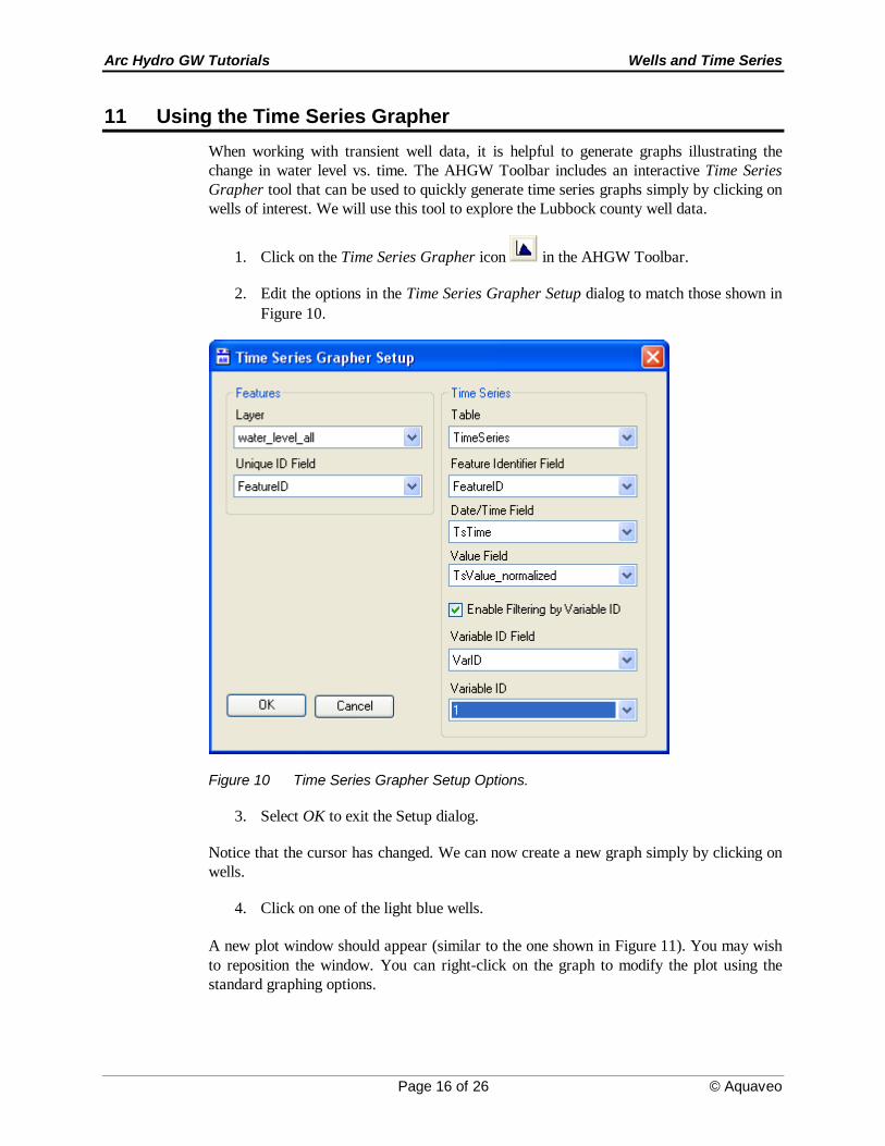
1. Click on the Time Series Grapher icon in the AHGW Toolbar.

2. Edit the options in the Time Series Grapher Setup dialog to match those shown in

‎Figure 10.

Figure 10 Time Series Grapher Setup Options.

3. Select OK to exit the Setup dialog.

Notice that the cursor has changed. We can now create a new graph simply by clicking on

wells.

4. Click on one of the light blue wells.

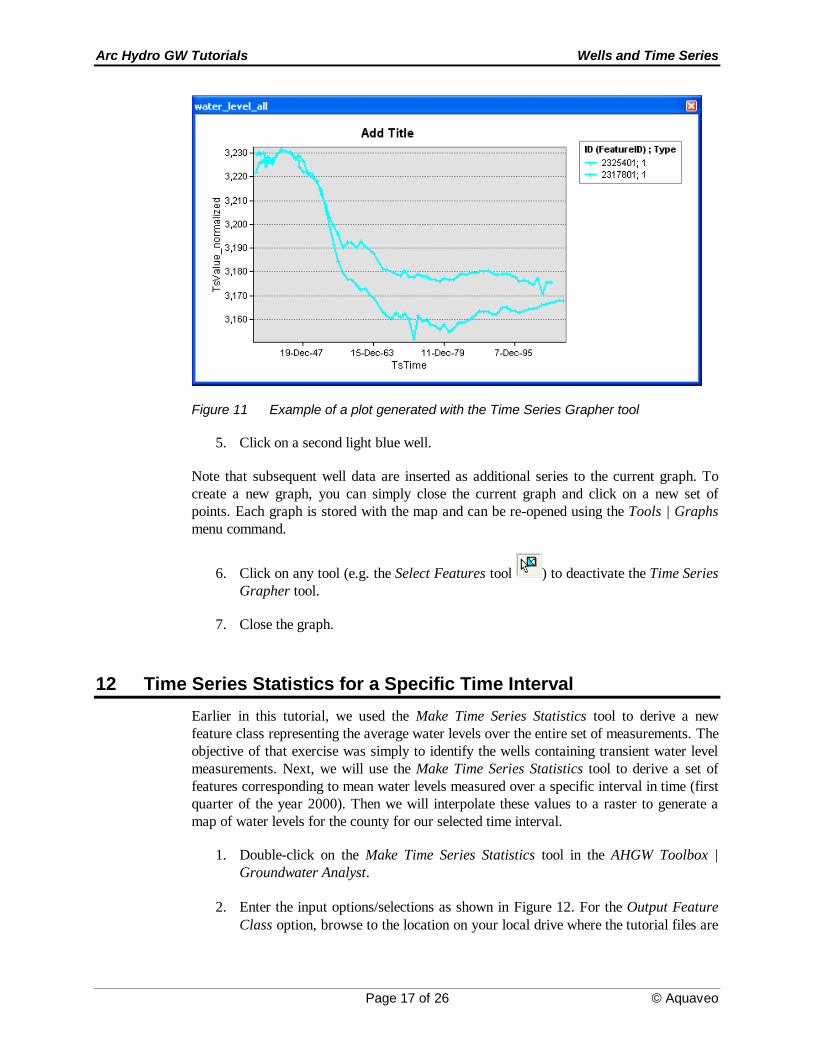
A new plot window should appear (similar to the one shown in ‎Figure 11). You may wish

to reposition the window. You can right-click on the graph to modify the plot using the

standard graphing options.



Figure 11 Example of a plot generated with the Time Series Grapher tool

5. Click on a second light blue well.

Note that subsequent well data are inserted as additional series to the current graph. To

create a new graph, you can simply close the current graph and click on a new set of

points. Each graph is stored with the map and can be re-opened using the Tools | Graphs

menu command.

6. Click on any tool (e.g. the Select Features tool ) to deactivate the Time Series

Grapher tool.

7. Close the graph.

12 Time Series Statistics for a Specific Time Interval

Earlier in this tutorial, we used the Make Time Series Statistics tool to derive a new

feature class representing the average water levels over the entire set of measurements. The

objective of that exercise was simply to identify the wells containing transient water level

measurements. Next, we will use the Make Time Series Statistics tool to derive a set of

features corresponding to mean water levels measured over a specific interval in time (first

quarter of the year 2000). Then we will interpolate these values to a raster to generate a

map of water levels for the county for our selected time interval.

1. Double-click on the Make Time Series Statistics tool in the AHGW Toolbox |

Groundwater Analyst.

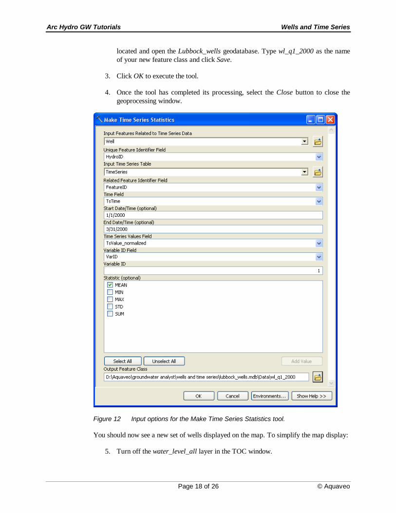
2. Enter the input options/selections as shown in ‎Figure 12. For the Output Feature

Class option, browse to the location on your local drive where the tutorial files are



located and open the Lubbock_wells geodatabase. Type wl_q1_2000 as the name

of your new feature class and click Save.

3. Click OK to execute the tool.

4. Once the tool has completed its processing, select the Close button to close the

geoprocessing window.

Figure 12 Input options for the Make Time Series Statistics tool.

You should now see a new set of wells displayed on the map. To simplify the map display:

5. Turn off the water_level_all layer in the TOC window.



13 Interpolating Water Levels

The next step is to interpolate the values from the new layer to a raster to generate a map

of water levels for Q1 of 2000. This step requires Spatial Analyst. If you do not have

Spatial Analyst installed, you will not be able to complete this part of the tutorial (you can

use the solution files to complete the tutorial). We will use the IDW geoprocessing tool to

perform the interpolation and we will set the Environment options such that the resulting

raster is clipped to the Lubbock County boundary.

1. Double-click on the IDW tool in ArcToolbox (located in the Spatial Analyst Tools

| Interpolation).

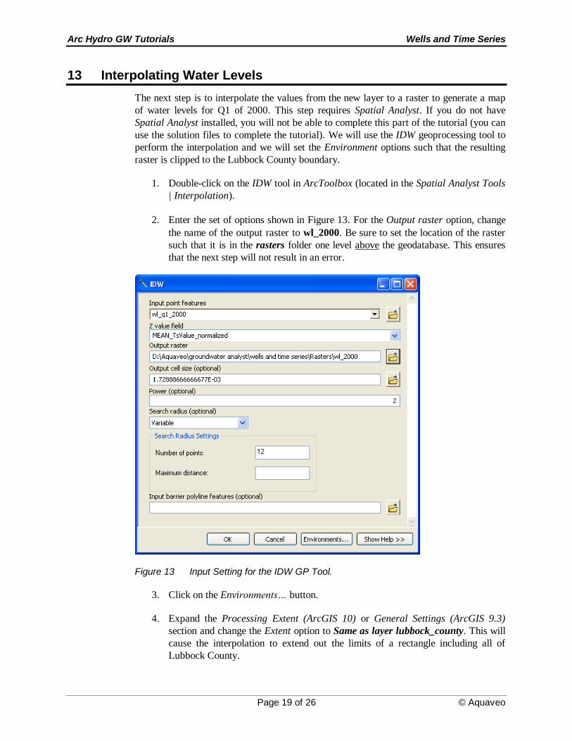
2. Enter the set of options shown in ‎Figure 13. For the Output raster option, change

the name of the output raster to wl_2000. Be sure to set the location of the raster

such that it is in the rasters folder one level above the geodatabase. This ensures

that the next step will not result in an error.

Figure 13 Input Setting for the IDW GP Tool.

3. Click on the Environments… button.

4. Expand the Processing Extent (ArcGIS 10) or General Settings (ArcGIS 9.3)

section and change the Extent option to Same as layer lubbock_county. This will

cause the interpolation to extend out the limits of a rectangle including all of

Lubbock County.



5. Scroll down and expand the Raster Analysis Settings section and change the Mask

option to lubbock_county. This will clip the raster to the actual boundary of

Lubbock County.

6. Select the OK button to exit the Environment Settings dialog.

7. Select the OK button to execute the IDW tool.

8. When the tool has finished, click on the Close button.

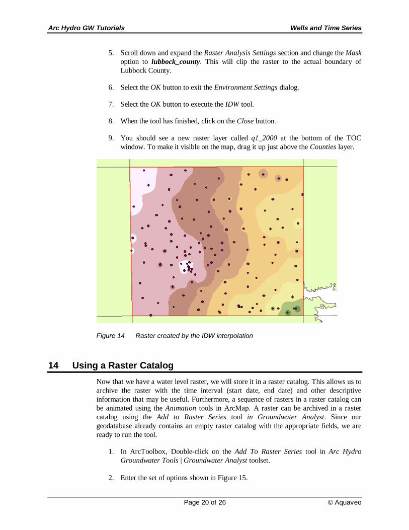
9. You should see a new raster layer called q1_2000 at the bottom of the TOC

window. To make it visible on the map, drag it up just above the Counties layer.

Figure 14 Raster created by the IDW interpolation

14 Using a Raster Catalog

Now that we have a water level raster, we will store it in a raster catalog. This allows us to

archive the raster with the time interval (start date, end date) and other descriptive

information that may be useful. Furthermore, a sequence of rasters in a raster catalog can

be animated using the Animation tools in ArcMap. A raster can be archived in a raster

catalog using the Add to Raster Series tool in Groundwater Analyst. Since our

geodatabase already contains an empty raster catalog with the appropriate fields, we are

ready to run the tool.

1. In ArcToolbox, Double-click on the Add To Raster Series tool in Arc Hydro

Groundwater Tools | Groundwater Analyst toolset.

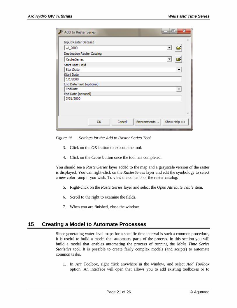
2. Enter the set of options shown in ‎Figure 15.



Figure 15 Settings for the Add to Raster Series Tool.

3. Click on the OK button to execute the tool.

4. Click on the Close button once the tool has completed.

You should see a RasterSeries layer added to the map and a grayscale version of the raster

is displayed. You can right-click on the RasterSeries layer and edit the symbology to select

a new color ramp if you wish. To view the contents of the raster catalog:

5. Right-click on the RasterSeries layer and select the Open Attribute Table item.

6. Scroll to the right to examine the fields.

7. When you are finished, close the window.

15 Creating a Model to Automate Processes

Since generating water level maps for a specific time interval is such a common procedure,

it is useful to build a model that automates parts of the process. In this section you will

build a model that enables automating the process of running the Make Time Series

Statistics tool. It is possible to create fairly complex models (and scripts) to automate

common tasks.

1. In Arc Toolbox, right click anywhere in the window, and select Add Toolbox

option. An interface will open that allows you to add existing toolboxes or to



create a new toolbox. Select the New Toolbox button (on the upper right). A

new toolbox should be added to the toolbox list. Select the new toolbox and select

the Open command. A new empty toolbox should be added to the Arc Toolbox

window.

2. Select the new toolbox, right click and select New Model. A new empty model

should be added to the toolbox.

3. Drag the Make Time Series Statistics tool into the model (you can also drag the

tool from the Results tab, this way you will already have the parameters defined in

the previous run set for the model).

You can expose tool parameters as model parameters. In this example we will set the input

feature classes, tables, and fields as constants and only expose the start date, end date, and

output features as model parameters.

4. Select the Make Time Series Statistics tool in the model, right click and select

Make Variable | From Parameter | Start Date. The Start Date parameter should

appear in the model as a circle

5. Do the same to add the End Date parameter to the model.

6. The parameters may appear on top of each other, you can select the Auto Layout

button to reorganize the parameters in the model display.

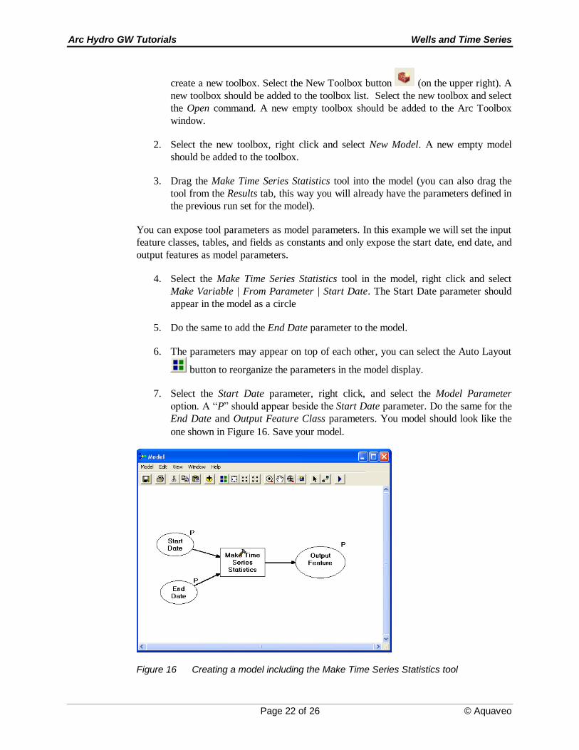
7. Select the Start Date parameter, right click, and select the Model Parameter

option. A “P” should appear beside the Start Date parameter. Do the same for the

End Date and Output Feature Class parameters. You model should look like the

one shown in ‎Figure 16. Save your model.

Figure 16 Creating a model including the Make Time Series Statistics tool



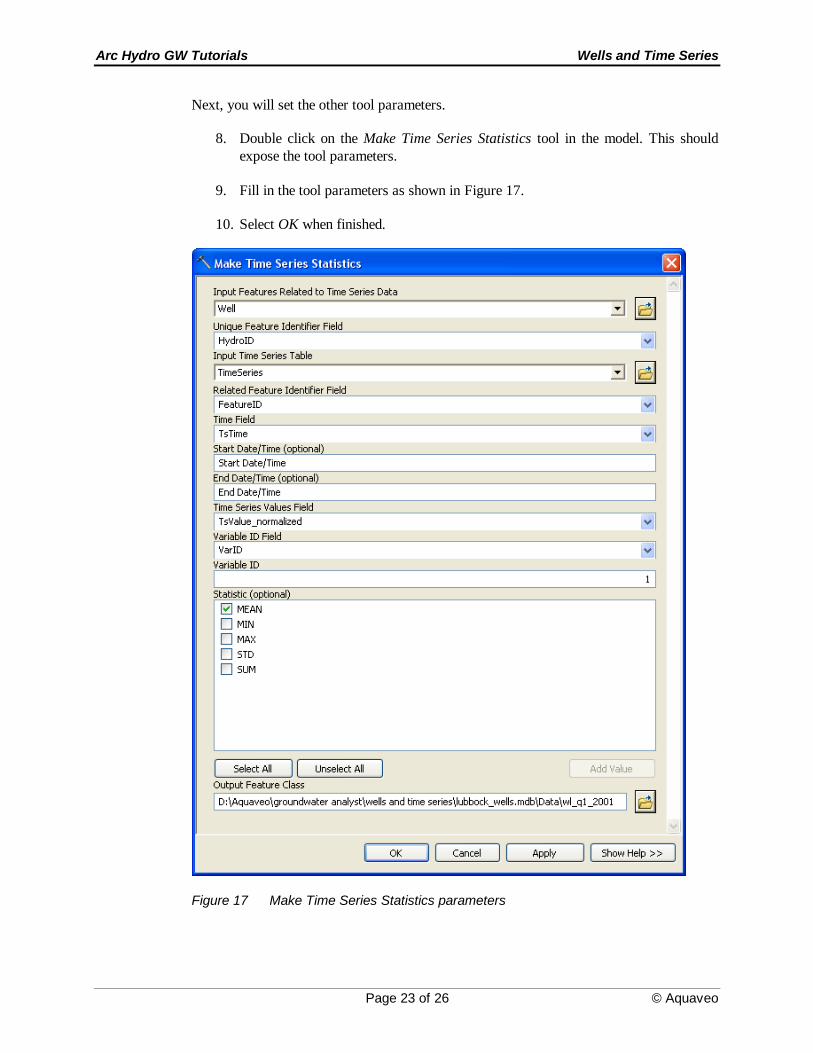
Next, you will set the other tool parameters.

8. Double click on the Make Time Series Statistics tool in the model. This should

expose the tool parameters.

9. Fill in the tool parameters as shown in ‎Figure 17.

10. Select OK when finished.

Figure 17 Make Time Series Statistics parameters



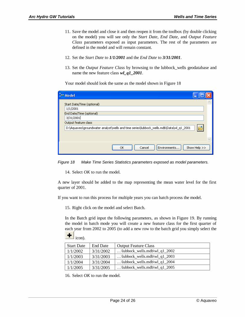
11. Save the model and close it and then reopen it from the toolbox (by double clicking

on the model) you will see only the Start Date, End Date, and Output Feature

Class parameters exposed as input parameters. The rest of the parameters are

defined in the model and will remain constant.

12. Set the Start Date to 1/1/2001 and the End Date to 3/31/2001.

13. Set the Output Feature Class by browsing to the lubbock_wells geodatabase and

name the new feature class wl_q1_2001.

Your model should look the same as the model shown in ‎Figure 18

Figure 18 Make Time Series Statistics parameters exposed as model parameters.

14. Select OK to run the model.

A new layer should be added to the map representing the mean water level for the first

quarter of 2001.

If you want to run this process for multiple years you can batch process the model.

15. Right click on the model and select Batch.

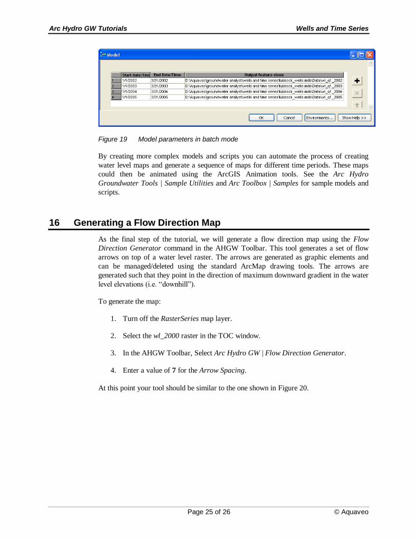
In the Batch grid input the following parameters, as shown in ‎Figure 19. By running

the model in batch mode you will create a new feature class for the first quarter of

each year from 2002 to 2005 (to add a new row to the batch grid you simply select the

icon).

Start Date End Date Output Feature Class

1/1/2002 3/31/2002 …\lubbock_wells.mdb\wl_q1_2002




16. Select OK to run the model.



Figure 19 Model parameters in batch mode

By creating more complex models and scripts you can automate the process of creating

water level maps and generate a sequence of maps for different time periods. These maps

could then be animated using the ArcGIS Animation tools. See the Arc Hydro

Groundwater Tools | Sample Utilities and Arc Toolbox | Samples for sample models and

scripts.

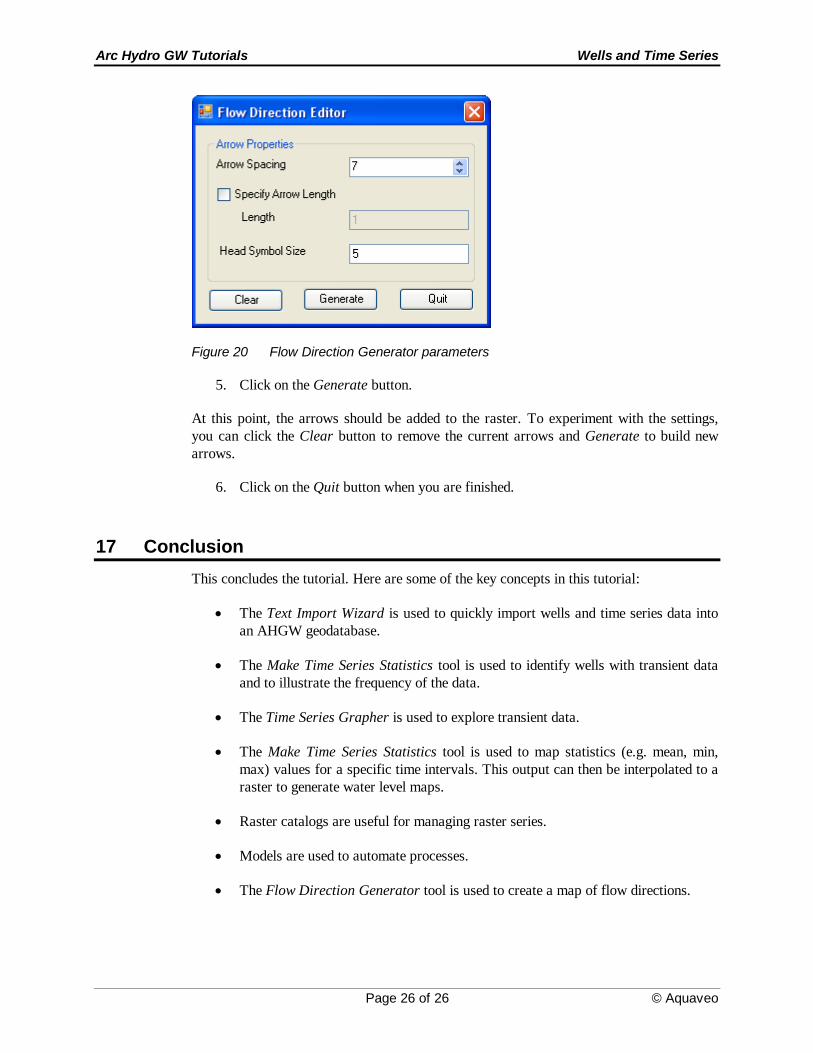
16 Generating a Flow Direction Map

As the final step of the tutorial, we will generate a flow direction map using the Flow

Direction Generator command in the AHGW Toolbar. This tool generates a set of flow

arrows on top of a water level raster. The arrows are generated as graphic elements and

can be managed/deleted using the standard ArcMap drawing tools. The arrows are

generated such that they point in the direction of maximum downward gradient in the water

level elevations (i.e. “downhill”).

To generate the map:

1. Turn off the RasterSeries map layer.

2. Select the wl_2000 raster in the TOC window.

3. In the AHGW Toolbar, Select Arc Hydro GW | Flow Direction Generator.

4. Enter a value of 7 for the Arrow Spacing.

At this point your tool should be similar to the one shown in ‎Figure 20.



Figure 20 Flow Direction Generator parameters

5. Click on the Generate button.

At this point, the arrows should be added to the raster. To experiment with the settings,

you can click the Clear button to remove the current arrows and Generate to build new

arrows.

6. Click on the Quit button when you are finished.

17 Conclusion

This concludes the tutorial. Here are some of the key concepts in this tutorial:

The Text Import Wizard is used to quickly import wells and time series data into

an AHGW geodatabase.

The Make Time Series Statistics tool is used to identify wells with transient data

and to illustrate the frequency of the data.

The Time Series Grapher is used to explore transient data.

The Make Time Series Statistics tool is used to map statistics (e.g. mean, min,

max) values for a specific time intervals. This output can then be interpolated to a

raster to generate water level maps.

Raster catalogs are useful for managing raster series.

Models are used to automate processes.

The Flow Direction Generator tool is used to create a map of flow directions.

Documents

Groundwater Analyst - Wells and Time Series - Aquaveo