Embed Size (px)
Citation preview

Mobile Robot Localization using Range Sensors : Consecutive Scanning and Cooperative Scanning 1
Mobile Robot Localization using Range Sensors : Consecutive Scanning
and Cooperative Scanning
Sooyong Lee and Jae-Bok Song
Abstract: This paper presents an obstacle detection algorithm based on the consecutive and the cooperative range sensor scanning schemes. For a known environment, a mobile robot scans the surroundings using a range sensor that can rotate 360 ° . The environment is rebuilt using nodes of two adjacent walls. The robot configuration is then estimated and an obstacle is detected by comparing characteristic points of the sensor readings. In order to extract edges from noisy and inaccurate sensor readings, a filtering algorithm is developed. For multiple robot localization, a cooperative scanning method with sensor range limit is developed. Both are verified with simulation and experiments. Keywords: Consecutive scanning, cooperative scanning, localization, mobile robot.
1. INTRODUCTION
Development of a fast and adaptive algorithm for avoiding moving obstacles has been one of the major interests in the mobile robot research area. To accomplish this objective, studies such as localization, obstacle detection and navigation have been done. The most fundamental requirement in dealing with the mobile robot is to precisely determine its configuration, which is localization. One of the most common ideas for estimating the current configuration is dead-reckoning using internal sensors such as the encoders attached to the wheels. The accuracy, however, decreases as the robot travels because dead reckoning leads to accumulation of draft errors mainly due to slip [1,2]. Periodic localization is required to correct these errors.
If environment scanning is performed at two different locations (consecutive scanning), changes in the environment are detected. Furthermore, if the travel distance is very small and also identified so that the systematic errors are ignored, then the relative change of the environment with respect to the mobile robot is extracted. The main purpose of this paper is to find useful applications for the consecutive scanning in mobile robot localization and navigation. If an
obstacle is present, the environment information includes the obstacle and the obstacle is differentiated from the consecutively scanned data set. If an obstacle is detected during both scanning procedures, the velocity of the obstacle is estimated and the obstacle position and velocity information is used for mobile robot navigation.
[3] showed that the odometry data are fused with the absolute position measurements to provide better and more reliable position estimation. Many landmark based or map based algorithms have been proposed by using range sensors [4,5]. As the vision technology develops, vision sensors are being widely used for mobile robot localization and navigation. [6] applied the landmark positioning idea to the vision sensor system for 2-Dimensional localization using a single camera. [7] developed a method that uses a stereo pair of cameras to determine the correspondence between the observed landmarks and the pre-loaded map and to estimate the 2-D location of the sensor from the correspondence. After a special mirror attached to a camera was developed, it became effortless to obtain an omni-directional view from a single camera [8]. With this omni-directional vision image, [9] proposed a fusion method for the vision image and sonar sensor information to compensate each other.
Even though using a vision sensor or combination of vision sensor and sonar sensor can provide us plenty of information about the environment, extraction of visual features for positioning is not easy. Furthermore, the time consumed to calculate the information restricts the speed of the mobile robot. [10,11] introduced a fast localization algorithm for mobile robots with range sensors. The workspace is partitioned into sectors and localization is done by comparing the identified labels with the predefined
__________ Manuscript received June 24, 2004; revised February 4, 2005; accepted February 4, 2005. Recommended by Editor Keum-Shik Hong. This work was supported by Grant No. (R01-2003-000-10336-0) from the Basic Research Program of the Korea Science & Engineering Foundation.
Sooyong Lee is with the Department of Mechanical Engineering, Hongik University, 72-1 Sangsu-Dong, Mapo-Gu, Seoul 121-791, Korea (e-mail: [email protected]). Jae-Bok Song is with the Department of Mechanical Engineering, Korea University, Anam-dong, Seongbuk-gu, Seoul 136-713, Korea (e-mail: [email protected]).
International Journal of Control, Automation, and Systems, vol. 3, no. 1, pp. 1-14, March 2005

2 Sooyong Lee and Jae-Bok Song
label information for the known environment. We propose the Consecutive Scanning Scheme for
mobile robot localization and navigation in the development of an environment change detection algorithm and efficient localization in a dynamic environment.
Not a single robot, but a team of miniature mobile robots is localized using ultrasonic range sensors in [12]. The localization method used in [12] was effective in simulation, but the ultrasonic range sensor's close proximity to the floor created some difficulty in processing experimental data. This method employed dead-reckoning in conjunction with the sensor data. It has a fair amount of accuracy and is inexpensive to implement. One drawback to the approach is that the initial position of each robot must be known.
Multiple robots equipped with laser range sensors are used to create a three dimensional map of an environment in [13]. Laser range sensors are used in conjunction with an omnidirectional video camera in [14]. The sensor data are compared to the environment map for localization. Laser sensors offer accurate readings of the environment and have longer effective ranges than infrared or ultrasonic sensors. However, they are far more expensive.
The second objective of our research is to develop a method for the localization of multiple mobile robots equipped with inexpensive range sensors (a rotating infrared sensor and a rotating CMOS camera) in a known indoor environment. It's assumed the environment contains straight edges and vertices only. Through the use of multiple robots, the limited range of inexpensive range sensors can be overcome and localization becomes possible. The multiple mobile robot system is treated as a linked robot for localization. This requires an unobstructed line of sight between each pair of robots forming a link. An individual robot cannot extract any useful information for global localization, solely from individual local sensing due to its limited sensing range. Thus, by considering the sensor reading generated by all the robots as one big virtual sensor, we have successfully shown that the robots can be separately localized.
The initial step of the localization process is to process the sensor scan data. It is necessary to locate any corners and saturation points in the data. Using this information, the Cartesian offsets can be determined. Next, a list of potential locations is generated for each robot. Using the relative distance and heading information, potential location pairs for the robots can be determined. Once a potential location pair has been found, it is checked for a line of sight; if one exists, the absolute heading for each robot is calculated.
The sector based range sensor data analysis is introduced in the following section. In Section 3,
sensor data filtering algorithm is explained to deal with sensor noise and inaccurate sensor reading. Consecutive scanning and cooperative scanning are described in Sections 4 and 5, respectively. Experimental results are shown in Section 6 followed by the conclusion.
2. SECTOR BASED RANGE SENSOR DATA
ANALYSIS Precise determination of the location of a mobile
robot is a fundamental requirement in controlling the mobile robot. In a planar motion, localization requires information about a robot’s position (x and y coordinates) and orientation (Θ ). Fig. 1(a) shows an infrared sensor mounted on a stepper motor.
By rotating the motor, the sensor can scan the environment. Fig. 2(a) is a simulated sensor reading in the environment shown in Fig. 1(b). The center is the origin of the sensor coordinates. If measured N times for 360° , the resolution is 360
N° and the i-th sensor
reading gives distance information at its angle with respect to the local coordinate (sensor coordinate). Fig.
(a) Rotating sensor.
(b) Consecutive scanning in an environment.
Fig. 1. Sensor and environment setup.

Mobile Robot Localization using Range Sensors : Consecutive Scanning and Cooperative Scanning 3
(a) Simulated sensor reading.
(b) Sensor data analysis.
Fig. 2. Single shot sensing.
Fig. 3. Visibility sectors.
2(b) shows the scanned sensor data. From this data, local minimum (m), local maximum (M) and discontinuity (D: contiguous points in the sequence of distance readings whose distance measurements differ by some predetermined threshold) points are identified
Table 1. Sector labels for the environment. Sector Label
1 mDCmMmMmMmM 2 mDCMmMmMmMmM 3 mMmMmMmMmMmM 4 mMmMmMmMmMCD 5 mMmMmMmMmCD 6 mMmDCMmMCDmM 7 mMmDCMmCDmM 8 mMmDCmMCDmM 9 mMmDCmCDmM
to characteristic points. C implies a connection point (the landing point for visibility ray passing by a discontinuity point), which is an additional characteri-stic point. For the scanning location shown in Fig. 2(b), the label sequence is mDCMmMmMmMmM. With this sequence, the sector of the mobile robot is determined, and orientation and position are calculated based on this sector information. For a given environment, the visibility analysis partitions the environment into sectors and each sector has a unique label sequence. Fig. 3 and Table 1 present the partitioned environment and the corresponding labels. According to Table 1 and Fig. 3, the environment shown in Fig. 2(a) contains 9 different sectors that each have their own unique labels.
Once the sector containing the robot is identified, we determine the position and orientation of the robot in that sector, i.e. we must determine its configuration ( , , )x y Θ . Note that we are aware of the world coordinates of the vertices and edges visible in this sector. In addition, we have sensor readings for each visible edge, and moreover, after the label matching, we know the edge associated with each distance measurement. If our sensor readings corresponding to the local maxima M characteristic points exactly coincided with the corresponding vertices of the environment, then localization would be trivial.
Let ( , )M MX Y and ( , )M Mx y denote the coordinates of the scanned local maximum point in the world and the robot’s local coordinate systems ( , )X Y and ( , )r rX Y , respectively. Then, the robot configuration ( , , )x y Θ denotes the linear transformation from ( , )X Y to ( , )r rX Y with translation ( , )x y and rotation ( )Θ , which can be represented as follows:
cos sinsin cos0 0 1 1 1
M M
M M
X x xY y y
− Θ Θ − Θ − Θ =
. (1)
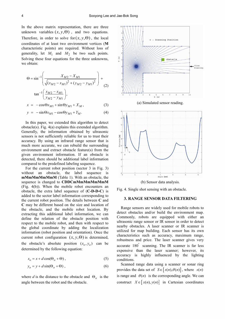
4 Sooyong Lee and Jae-Bok Song
In the above matrix representation, there are three unknown variables ( , , )x y Θ , and two equations. Therefore, in order to solve for ( , , )x y Θ , the local coordinates of at least two environment vertices (M characteristic points) are required. Without loss of generality, let 1M and 2M be two such points. Solving these four equations for the three unknowns, we obtain:
1 2 12 2
2 1 2 1
sin ( ) ( )
M M
M M M M
X X
x x y y− − Θ = + − + − (2)
1 2 1
2 1tan M M
M M
x xy y
− − −
,
1 1 cos sinM M Mx x y X= − Θ + Θ + , (3)
1 1 sin cos .= − Θ − Θ +M M My x y Y (4)
In this paper, we extended this algorithm to detect obstacle(s). Fig. 4(a) explains this extended algorithm. Generally, the information obtained by ultrasonic sensors is not sufficiently reliable for us to trust their accuracy. By using an infrared range sensor that is much more accurate, we can rebuild the surrounding environment and extract obstacle feature(s) from the given environment information. If an obstacle is detected, there should be additional label information compared to the predefined labeling sequence.
For the current robot position (sector 3 in Fig. 3) without an obstacle, the label sequence is mMmMmMmMmM (Table 1). With an obstacle, the sequence is changed to CDDCmMmMmMmMmM (Fig. 4(b)). When the mobile robot encounters an obstacle, the extra label sequence of (C-D-D-C) is added to the sector label information corresponding to the current robot position. The details between C and C may be different based on the size and location of the obstacle, and the mobile robot location. By extracting this additional label information, we can define the relation of the obstacle position with respect to the mobile robot, and then with respect to the global coordinate by adding the localization information (robot position and orientation). Once the current robot configuration ( , , )x y Θ is determined, the obstacle’s absolute position ( , )o ox y can be determined by the following equation:
cos( )o ox x d= + Θ + Θ , (5)
sin( ) ,= + Θ +Θo oy y d (6)
where d is the distance to the obstacle and oΘ is the angle between the robot and the obstacle.
(a) Simulated sensor reading.
(b) Sensor data analysis.
Fig. 4. Single shot sensing with an obstacle.
3. RANGE SENSOR DATA FILTERING Range sensors are widely used for mobile robots to
detect obstacles and/or build the environment map. Commonly, robots are equipped with either an ultrasonic range sensor or IR sensor in order to detect nearby obstacles. A laser scanner or IR scanner is utilized for map building. Each sensor has its own characteristics such as accuracy, maximum range, robustness and price. The laser scanner gives very accurate 180° scanning. The IR scanner is far less expensive than the laser scanner; however, its accuracy is highly influenced by the lighting conditions.
Scanned range data using a scanner or sonar ring provides the data set of [ ]( ), ( )S s n nθ∈ , where ( )s n is range and ( )nθ is the corresponding angle. We can construct [ ]( ), ( )X x n y n∈ in Cartesian coordinates

Mobile Robot Localization using Range Sensors : Consecutive Scanning and Cooperative Scanning 5
from S . It is commonly observed that the constructed data doesn't form an edge even though the sensor rays hit a single edge due to sensor error.
In this paper, we use either concave corner or convex corner or an edge for localization. Therefore, it is very important to extract corners or edges from the sensor data even with errors. This section describes how to process range sensor data to find edges. If there are two connected edges, they are regarded as a corner.
Finding the edge is regarded as finding a line that best fits ( ):X i j samples. Simple linear regression is employed to find the line equation of the edge in Cartesian coordinates. The results from the linear regression are 1a and 0a in 1 0y a x a= + . In case the residual mean square value, rS is too large, the samples used to form an edge are invalid. Before applying the linear regression to the sampled data set, we first group them into subgroups by calculating the metric distance between two nearby samples. Large distance is usually due to visibility. We start by using three consecutive samples to find out a line parameter
1a from linear regression and also rS . Then we
Table 2. Filtering algorithm.
include the next sample from the same subgroup and check how much rS is changed. If the change is small enough, the newly added sample is included in the subgroup, that is, same edge. If not, the newly added sample is not from the same edge. However, it is necessary to add another subsequent sample, remove the previously added one and check rS because there may exist one false sensor reading.
Once the subdivision based on linear regression is finished, then merging the successive subgroups is necessary, thus noisy data is filtered out from an edge. This is done by comparing the slopes of two nearby subgroups (now, they are two edges and 1a values of two nearby edges are compared). If the difference is small enough, then two subgroups are merged into one. The algorithm is described in Table 2.
The objective of filtering is to extract edges from the range sensor data even with sensor noise and sensor inaccuracy. In order to verify the proposed algorithm, experimental range sensor data added with random 5%± sensor noise in a small T-shaped environment is processed. Fig. 5 indicates how the filtering works with noisy sensor data. The sensor is located at the origin (0,0) and from 360 ° scanning, we can construct the points where the sensor rays hit in Cartesian coordinates. We set the magnitude of the random noise proportional to the distance. Fig. 5(a) shows the grouping of the points from linear regression. The numbers refer to the group numbers. Even on an edge, there are several groups and the identified edges are shown in Fig. 5(b). With repeated merging based on 10) in Table 2, the edges are identified as shown in Fig. 5(d). Note that the final edges are not exactly T-shaped because the sensor data includes random noise. With this filtered data, it is possible to apply the sector based range data analysis described in Section 2. If there are two connected edges, there exist a corner in-between and the corner can be identified as either convex or concave from the difference between the two edges.
4. CONSECUTIVE SCANNING SCHEME By comparing two data sets obtained from the
consecutive scanning scheme, we can extract moving obstacle information. From two data sets, the velocity of the obstacle can be estimated. The sensing data, however, doesn’t exactly represent the positions of the obstacles, because we know the limited number of sensor scanning and the sensor ray may/may not hit the obstacle, depending on the shape and size of the obstacle(s). As the robot moves along the predetermined path, it could encounter an unexpected obstacle(s). After a short period of time, the second scanning is performed. Fig. 6(a) shows the robot movement and the obstacle movement. The robot scans
Input: [ ]( ), ( )S s n nθ∈ Output: Groups of samples that form edges, slope of edges 1) Construct [ ]( ), ( )X x n y n∈ from S 2) Initial grouping: 3) Generate initial group, ( )G m with
1( ) ( 1)X i X i ε− + > where ( ) ( )X i G j∈ and ( 1) ( 1)X i G j+ ∈ +
4) Subdivision: 5) Subdivide each group by linear regression 6) While 2( : , 1) ( : , )r rS k l l S k l l ε+ − < 7) Add ( 1)X i + to current subgroup 8) If 2( : , 2) ( : , )r rS k l l S k l l ε+ − < then
neglect ( 1)X i + and proceed with current subgroup
9) Merge: 10) If 1 1 3( ) ( 1)a m a m ε− + < then combine
( )G m and ( 1)G m + 11) Repeat 10) * rS : Residual Mean Square * 1()a : Slope of the line from linear regression * 1 2 3, ,ε ε ε : Threshold values

6 Sooyong Lee and Jae-Bok Song
(a) Grouping of noisy range sensor data.
(b) Edges found from the initial linear regression.
(c) Merged edges (1st).
(d) Merged edges (2nd).
Fig. 5. Filtering noisy sensor data.
the environment at the first location and again at the second location after small movement. The range sensor readings are presented in Fig. 6(b). The origin of the polar plot (radial distance is the range sensor data in [m] and the angle is shown in [degree]) is the robot center.
These consecutive data sets are also used in performing localization and obtaining obstacle information. The position and velocity of the obstacle can be estimated by comparing two data sets. Comparing two data sets can give us additional details about the position and orientation of the mobile robot because the robot moves a certain amount of distance in the consecutive scanning scheme. Let’s assume that we command the robot to move small amount of
(a) Robot with a moving obstacle.
(b) Comparison of two data sets.
Fig. 6. Consecutive scanning.

Mobile Robot Localization using Range Sensors : Consecutive Scanning and Cooperative Scanning 7
movement ( ),d∆ so that we can disregard the odometry errors. After obtaining two data sets and characteristic points for each set, we can get the robot movement vector whose magnitude is d∆ and direction is Θ . Redundant information of other non-varying characteristic points would be helpful to precise localization. Fig. 7 shows the data comparison method between two scanned data sets.
Let us define P1 and P2 as the first scanning and second scanning position, respectively. [ ]1r i represents the range sensor reading of i-th scanned data at P1 and [ ] [ ]1 1( , )x i y i is the configuration with respect to robot local coordinate system at P1. [ ]2r i ,
[ ] [ ]2 2( , )x i y i are for the secondly scanned data set. d∆ is the travel distance of the mobile robot
predetermined by the consecutive scanning scheme. d∆ is set small enough so that we can ignore the
odometry error while the robot is moving from P1 to P2. Note that the data comparison is made at the same angle [ ]iθ for i-th scanned data because the robot moves forward, which means the first and the second robot local coordinates share the same X-axis. [ ]x i∆ and [ ]y i∆ are the changes of the i-th scanned data at P1 and P2 respectively, and can be calculated by
[ ] [ ] [ ] [ ] [ ]1 2cos cosx i r i i r i i dθ θ∆ + = + ∆ , (7)
[ ] [ ] [ ] [ ] [ ]2 1sin siny i r i i r i iθ θ∆ + = . (8)
If [ ]jφ is known prior to the comparison from localization, [ ]x i∆ and [ ]y i∆ can be derived from the geometric configuration in Fig. 7 as:
[ ] [ ] [ ][ ] [ ]
sin cossin( )
i jx i d
i jθ φθ φ
∆ = ∆+
, (9)
[ ] [ ] [ ][ ] [ ]
sin sinsin( )
i jy i d
i jθ φθ φ
∆ = ∆+
. (10)
If there is no change in the environment, the following relation should be held. Otherwise, we can extract the obstacle location from the two consecutive scanning data sets with
[ ] [ ] [ ]1 2x i x i d x i= + ∆ − ∆ , (11)
[ ] [ ] [ ]1 2y i y i y i= + ∆ . (12)
There are two cases in which the above relations ((11) and (12)) are not satisfied. • [ ] [ ]1 1( , )x i y i and [ ] [ ]2 2( , )x i y i are not on the
same edge. • There exists a moving obstacle(s). In case the above relations are not satisfied, (11) and (12) are written as
[ ] [ ] [ ]1 2xD x i x i d x i= − − ∆ + ∆ , (13)
[ ] [ ] [ ]1 2yD y i y i y i= − − ∆ , (14)
2 2x yD D D= + . (15)
Therefore, from the consecutive scanning, we can easily find out the nodes and/or the location of moving obstacle(s) from non-zero D in (15).
Different from the conventional scanning method that focuses on the single scan data, the consecutive scanning scheme compares two successive scan data, which are measured at two close locations. More importantly, the movement in-between two measurements is planned accordingly so that there doesn’t exist any dead-reckoning error. Therefore, it provides much more information than the single scan that only detects the current environment information.
Fig. 8(a) shows the value D for the first case. Eight node locations are identified from this figure. Fig. 8(b) is the experimental result in the same environment as in Fig. 8(a), but with an obstacle. Due to an obstacle, the large value of D is shown at 315 ° . It should be noted that the value indicates the distance from the edge to the obstacle, not the distance from the robot to the obstacle. However, the location of the obstacle can be computed with the sensor data from (5) and (6).
5. COOPERATIVE SCANNING SCHEME
The mobile robot localization method treats the
robots as a linked system whereby the distance between the robot centers and relative headings are recognized. This information can be found via an omnidirectional camera or by maintaining the distance between the robots within the range sensors' effective range. This necessitates a line of sight between each successive robot in the system. Fig. 7. Data comparison.

8 Sooyong Lee and Jae-Bok Song
The distance between the robots will be found via a sensor - an omnidirectional sensor may be used - and is represented as RD . The maximum limit of the range sensor is
maxSR . The effective range of the sensor used to determine the distance between the robots is given by
minDR and maxDR . Initially, it will
be assumed that max maxS R DR D R< < and
minR DD R≥ . Once a method has been developed under the previous governing assumption, it will be tested under the condition
max maxS R SR D R< < - the situation where the second sensor would be unnecessary. Fig. 9 illustrates a T-shaped environment containing two robots; each robot can only detect a small portion of the environment. A localization method based on detecting the corners in the environment from each robot's range sensor scan has been tested. The approach has been simulated for two robots and thus far incorporates the relative distance information but not the relative
heading information. The currently implemented localization method is: 1) Filter the sensor data shown in Table 2. 2) Find the concave and convex corners in the sensor
scan for each robot. 3) Generate a list of the possible locations for each
robot in the environment. 4) For each possible location of the first robot, check
the distance between that point and each of the second robot's possible locations. If the distance between a pair of points is equal to the known distance between the robots, the pair provides the potential locations of the two robots.
5) Check each potential location pair for a line of sight. If one is found, the pair is retained.
6) For each remaining possible location pair, conduct a simulated sensor scan of the environment. Compare the scans to the original sensor scans. The possible location pair with the smallest error is deemed to give the location of the pair of robots.
The order of the steps is determined by the computation time required. Checking a pair of robot locations for a line of sight takes significantly longer than calculating the distance between two potential locations. Hence, the distance criterion is used to reduce the set of possible location pairs to check for a line of sight, thereby reducing computation time. The above method is limited in that it is unable to determine the exact configuration of the robots in an environment in which there are potential symmetric configurations. It also does not make full use of the relative heading information that is necessary to determine each robot's heading. An additional constraint is that each robot must detect at least one corner of the environment.
(a) Simulation.
(b) Experiment.
Fig. 8. Consecutive scanning simulation and experi-ment.
Fig. 9. T-Shaped environment with two robots.
Mobile Robot Localization using Range Sensors : Consecutive Scanning and Cooperative Scanning 9
The next step will be to incorporate the relative heading information that can be determined from the sensor readings. This will be initially implemented on a one-link system (two robots). Incorporating the relative heading information will allow for the determination of the robots' absolute headings. For more than two robots the relative heading information will be used to determine the joint angle. Fig. 10 shows the environment with three robots, which will be regarded as a two-link robot.
The first step in the proposed localization method is to determine the link length and relative angle for each successive pair of robots from the sensor information. For systems with more than two robots, the joint angles (θ ) can be determined. Incorporating the relative heading information with the range sensor data from each robot, it is expected that the absolute orientation of the robot system can be narrowed down to a few configurations (the exact location will not be able to be determined as this method will not require a corner to be found by each robot). Potential robot locations will be determined by searching either the workspace or the C-space.
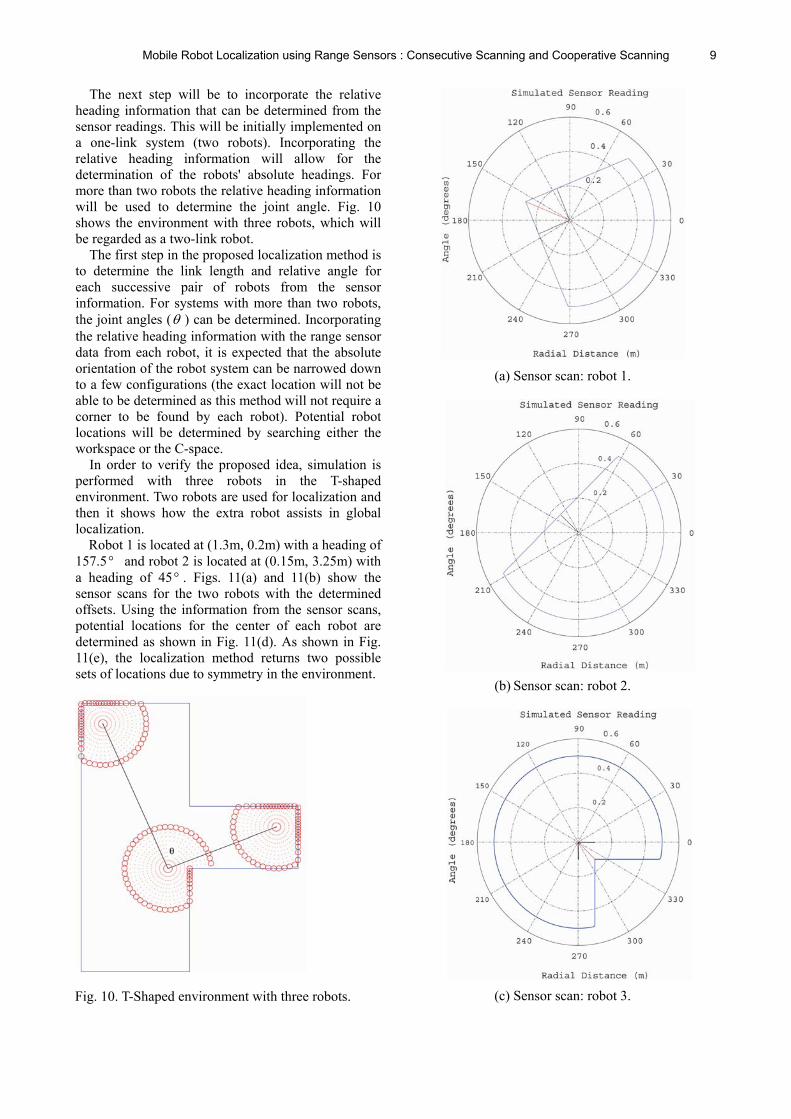
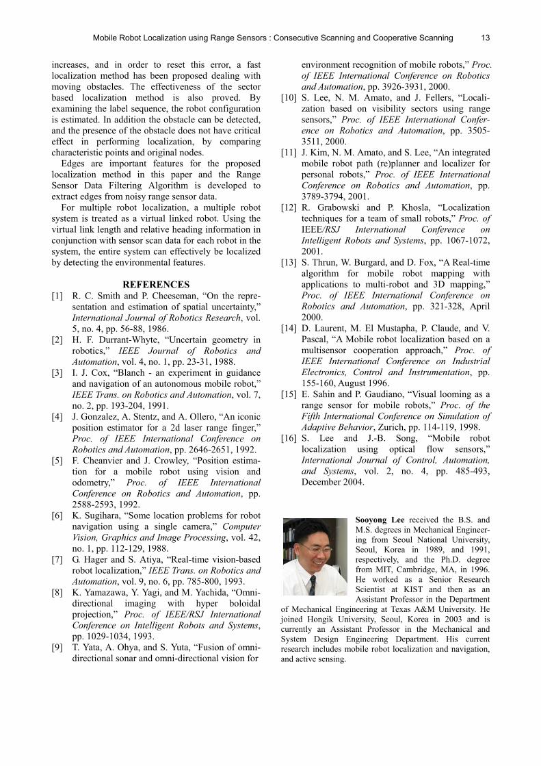
In order to verify the proposed idea, simulation is performed with three robots in the T-shaped environment. Two robots are used for localization and then it shows how the extra robot assists in global localization.
Robot 1 is located at (1.3m, 0.2m) with a heading of 157.5 ° and robot 2 is located at (0.15m, 3.25m) with a heading of 45 ° . Figs. 11(a) and 11(b) show the sensor scans for the two robots with the determined offsets. Using the information from the sensor scans, potential locations for the center of each robot are determined as shown in Fig. 11(d). As shown in Fig. 11(e), the localization method returns two possible sets of locations due to symmetry in the environment.
(a) Sensor scan: robot 1.
(b) Sensor scan: robot 2.
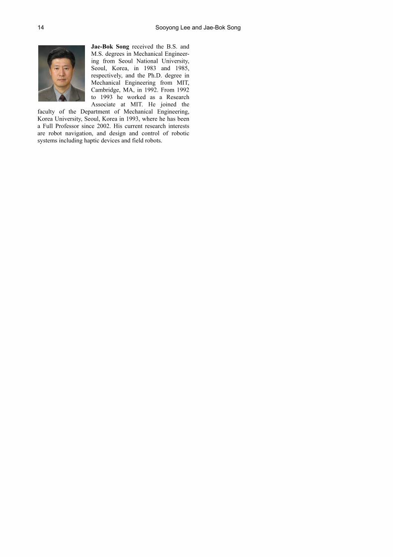
(c) Sensor scan: robot 3.
Fig. 10. T-Shaped environment with three robots.

10 Sooyong Lee and Jae-Bok Song
In this scenario, a third robot could be used to uniquely localize the robot system. If a third robot is added at (1.4m, 2.4m) with a heading of 90 ° , a unique location can be determined for each robot. Fig. 11(c) presents the sensor scan for the third robot with the calculated offsets. The possible locations for the second pair of robots, robots 2 and 3, are shown in Fig. 11(f). By finding the position of the second robot in the localization result for the first pair of robots (shown in Fig. 11(e)) corresponding to the location of the first robot in the result for the second pair of robots, a unique solution for the system of three robots is discovered as shown in Fig. 11(g).
6. EXPERIMENT
6.1. Consecutive scanning
DIRRS (Digital Infra-Red Ranging Sensor) is used for the experiment. Due to the sensor range limitation (10cm-80cm) and sensor resolution variation as the distance increases, this experiment is done in a 40cm × 60cm environment as shown in Fig. 1(b). A stepping motor with 0.9 degree resolution is used as the rotating actuator. With the stepping motor, the DIRRS obtains 400 scanned data for one complete rotation. Two consecutive scanning results without an obstacle are shown in Figs. 12(a) and 12(b), and those with an obstacle are in Figs. 13(a) and 13(b).
The sensor readings are translated into the local coordinate of the mobile robot and the edges are regenerated by the line regression, which minimizes RMS errors for each edge. Then, nodes from the line regression are expressed as the crossing point of two adjacent edges. Nodes obtained from the line regression are compared with the actual nodes in the environment. For this particular experiment, the label
(d) Possible locations for robots 1 and 2.
(e) Multiple localization results with two robots.
(f) Possible locations for robots 2 and 3.
(g) Unique localization solution.
Fig. 11. Simulation results.

Mobile Robot Localization using Range Sensors : Consecutive Scanning and Cooperative Scanning 11
is mMmMmMmMmMmM (refer to Fig. 3 and Table 1). For the consecutive scanning scheme, a 2cm travel command ( )d∆ is given to the mobile robot. The movement is made from (10cm, 30cm) to (11.4cm, 31.4cm) in the global coordinate so that the direction of the movement is 45 ° . Localization for the first scanning without an obstacle (Fig. 12(a)) is (10.4cm, 29.5cm, 44.5 ° ) while the actual configuration is (10cm, 30cm, 45 ° ). At the second position without an obstacle (Fig. 12(b)), the estimated configuration of the mobile robot is (11.1cm, 30.7cm, 44 ° ) where (11.4cm, 31.4cm, 45 ° ) is the actual configuration. In the dynamic environment (Figs. 13(a) and 13(b)), a moving obstacle is detected as approaching the robot
(a) First scanning.
(b) Second scanning.
Fig. 12. Consecutive scanning without an obstacle.
(a) First scanning.
(b) Second scanning.
Fig. 13. Consecutive scanning with an obstacle.
Table 3. Experimental results of localization and obstacle detection.
Case Actual Configuration
Estimated Configuration
Localization 1
(10.4cm, 29.5cm, 44.5 ° )
(11.4cm, 31.4cm, 45.0 ° )
Localization 2
(11.1cm, 30.7cm, 44.0 ° )
(11.4cm, 31.4cm, 45.0 ° )
Obstacle 1 (31.0cm, 30.5cm) (29.8cm, 32.4cm)
Obstacle 2 (29.0cm, 30.5cm) (28.3cm, 34.3cm)

12 Sooyong Lee and Jae-Bok Song
at an angle of 314 ° . The obstacle movement is extracted as it moves from (29.8cm, 32.4cm) to (28.3cm, 34.3cm) in the global coordinate while the center of the obstacle moves (31.0cm, 30.5cm) to (29.0cm, 30.5cm). 6.2 Cooperative scanning
To find the distance and heading angle between robots, we have used a CMOS camera. The image size is 80×143 pixels and allows for serial communication with a PC or a microcontroller. The camera is mounted on a stepper motor and the image processing component of the camera can successfully track an object of a given color at 15 fps. The encoder reading from the stepper motor provides us with the relative heading between two robots and an extension of “the Looming effect” provides us with the distance to the other robot. Extracting the depth of an object from an image using visual looming techniques is dealt with in [15]. Calculating the width of the image through Looming is easier and computationally less complex than using stereoscopic imaging.
An inexpensive infrared range sensor with a nominal effective radius of 10-80 cm was used to measure the radial distance from the robot center to the walls of the environment. The principal concern initially was the effective determination of the environmental features, which is critical to effective localization.
Robot 1 was placed at (0.65m, 0.85m) with a 180 ° heading and robot 2 was placed at (0.1m, 0.1m) with a 180 ° heading. Figs. 14 and 15 indicate the filtered sensor scans and the determined corner point for robots 1 and 2 respectively. Using the information from the sensor scans in addition to the virtual link length and relative heading information, the robots can be accurately localized. Fig. 16 shows the expected locations for robots 1 and 2 in the T-Shaped
environment. Table 4 compares the experimental results of the two robots to the nominal values. The specification of the robots used for the experiments is given in [16].
7. CONCLUSIONS
In this paper, the usefulness of the consecutive
scanning scheme and cooperative scanning scheme for mobile robot localization and obstacle detection is presented. As the robot moves, the accumulated error
Fig. 15. Experimental sensor scan of concave corner.
Fig. 16. Experimental localization result.
Table 4. Experimental results.
Robot1 Robot2
Actual (0.65m,0.85m, 180 ° )
(0.10m,0.10m, 180 ° )
Estimated (0.64m,0.86m, 181 ° )
(0.10m,0.098m,181 ° )
Fig. 14. Experimental sensor scan of convex corner.
Mobile Robot Localization using Range Sensors : Consecutive Scanning and Cooperative Scanning 13
increases, and in order to reset this error, a fast localization method has been proposed dealing with moving obstacles. The effectiveness of the sector based localization method is also proved. By examining the label sequence, the robot configuration is estimated. In addition the obstacle can be detected, and the presence of the obstacle does not have critical effect in performing localization, by comparing characteristic points and original nodes.
Edges are important features for the proposed localization method in this paper and the Range Sensor Data Filtering Algorithm is developed to extract edges from noisy range sensor data.
For multiple robot localization, a multiple robot system is treated as a virtual linked robot. Using the virtual link length and relative heading information in conjunction with sensor scan data for each robot in the system, the entire system can effectively be localized by detecting the environmental features.
REFERENCES
[1] R. C. Smith and P. Cheeseman, “On the repre-sentation and estimation of spatial uncertainty,” International Journal of Robotics Research, vol. 5, no. 4, pp. 56-88, 1986.
[2] H. F. Durrant-Whyte, “Uncertain geometry in robotics,” IEEE Journal of Robotics and Automation, vol. 4, no. 1, pp. 23-31, 1988.
[3] I. J. Cox, “Blanch - an experiment in guidance and navigation of an autonomous mobile robot,” IEEE Trans. on Robotics and Automation, vol. 7, no. 2, pp. 193-204, 1991.
[4] J. Gonzalez, A. Stentz, and A. Ollero, “An iconic position estimator for a 2d laser range finger,” Proc. of IEEE International Conference on Robotics and Automation, pp. 2646-2651, 1992.
[5] F. Cheanvier and J. Crowley, “Position estima-tion for a mobile robot using vision and odometry,” Proc. of IEEE International Conference on Robotics and Automation, pp. 2588-2593, 1992.
[6] K. Sugihara, “Some location problems for robot navigation using a single camera,” Computer Vision, Graphics and Image Processing, vol. 42, no. 1, pp. 112-129, 1988.
[7] G. Hager and S. Atiya, “Real-time vision-based robot localization,” IEEE Trans. on Robotics and Automation, vol. 9, no. 6, pp. 785-800, 1993.
[8] K. Yamazawa, Y. Yagi, and M. Yachida, “Omni-directional imaging with hyper boloidal projection,” Proc. of IEEE/RSJ International Conference on Intelligent Robots and Systems, pp. 1029-1034, 1993.
[9] T. Yata, A. Ohya, and S. Yuta, “Fusion of omni-directional sonar and omni-directional vision for
environment recognition of mobile robots,” Proc. of IEEE International Conference on Robotics and Automation, pp. 3926-3931, 2000.
[10] S. Lee, N. M. Amato, and J. Fellers, “Locali-zation based on visibility sectors using range sensors,” Proc. of IEEE International Confer-ence on Robotics and Automation, pp. 3505-3511, 2000.
[11] J. Kim, N. M. Amato, and S. Lee, “An integrated mobile robot path (re)planner and localizer for personal robots,” Proc. of IEEE International Conference on Robotics and Automation, pp. 3789-3794, 2001.
[12] R. Grabowski and P. Khosla, “Localization techniques for a team of small robots,” Proc. of IEEE/RSJ International Conference on Intelligent Robots and Systems, pp. 1067-1072, 2001.
[13] S. Thrun, W. Burgard, and D. Fox, “A Real-time algorithm for mobile robot mapping with applications to multi-robot and 3D mapping,” Proc. of IEEE International Conference on Robotics and Automation, pp. 321-328, April 2000.
[14] D. Laurent, M. El Mustapha, P. Claude, and V. Pascal, “A Mobile robot localization based on a multisensor cooperation approach,” Proc. of IEEE International Conference on Industrial Electronics, Control and Instrumentation, pp. 155-160, August 1996.
[15] E. Sahin and P. Gaudiano, “Visual looming as a range sensor for mobile robots,” Proc. of the Fifth International Conference on Simulation of Adaptive Behavior, Zurich, pp. 114-119, 1998.
[16] S. Lee and J.-B. Song, “Mobile robot localization using optical flow sensors,” International Journal of Control, Automation, and Systems, vol. 2, no. 4, pp. 485-493, December 2004.
Sooyong Lee received the B.S. and M.S. degrees in Mechanical Engineer-ing from Seoul National University, Seoul, Korea in 1989, and 1991, respectively, and the Ph.D. degree from MIT, Cambridge, MA, in 1996. He worked as a Senior Research Scientist at KIST and then as an Assistant Professor in the Department
of Mechanical Engineering at Texas A&M University. He joined Hongik University, Seoul, Korea in 2003 and is currently an Assistant Professor in the Mechanical and System Design Engineering Department. His current research includes mobile robot localization and navigation, and active sensing.
14 Sooyong Lee and Jae-Bok Song
Jae-Bok Song received the B.S. and M.S. degrees in Mechanical Engineer-ing from Seoul National University, Seoul, Korea, in 1983 and 1985, respectively, and the Ph.D. degree in Mechanical Engineering from MIT, Cambridge, MA, in 1992. From 1992 to 1993 he worked as a Research Associate at MIT. He joined the
faculty of the Department of Mechanical Engineering, Korea University, Seoul, Korea in 1993, where he has been a Full Professor since 2002. His current research interests are robot navigation, and design and control of robotic systems including haptic devices and field robots.