Embed Size (px)
Citation preview

Mixture Modeling 1
Running Head: Mixture Modeling
Chapter 21
Mixture Modeling for Organizational Behavior Research
Order of Authorship and Contact Information
Alexandre J. S. Morin*
Substantive-Methodological Synergy Research Laboratory
Department of Psychology, Concordia University
7141 Sherbrooke W,
Montreal, QC, Canada, H4B 1R6
Phone: (+1) 514-848-2424 ext. 3533
Email: [email protected]
https://smslabstats.weebly.com/
Matthew J. W. McLarnon*
Department of Psychology
Oakland University
654 Pioneer Drive
Rochester, Michigan 44309
Phone: (+1) 248-370-2343
Email: [email protected]
David Litalien
Département des fondements et pratiques en éducation
Faculté des sciences de l'éducation, Université Laval
2320, rue des Bibliothèques, Office 938
Québec, QC, Canada, G1V 0A6
Phone: (+1) 418-656-3131 ext. 408699
Email: [email protected]
* The first two authors (AJSM & MJWM) contributed equally to this chapter and both should
be considered first authors.
Acknowledgements
The first and third authors were supported by a grant from the Social Science and Humanities
Research Council of Canada (435-2018-0368).
This is a draft chapter / article. The final version is will be available in the Handbook on the
Dynamics of Organizational Behavior edited by Y. Griep & S.D. Hansenpublished in 2020, Edward
Elgar Publishing Ltd
The material cannot be used for any other purpose without further permission of the publisher, and is
for private use only.
Morin, A.J.S., McLarnon, M.J.W., & Litalien, D. (2020). Mixture modeling for organizational
behavior research. In Y. Griep & S.D. Hansen (Eds.), Handbook on the Temporal Dynamics of
Organizational Behavior (pp. 351-379). Cheltenham, UK: Edward Elgar.

Mixture Modeling 2
Abstract
This chapter introduces mixture modeling, with a specific focus on the analytical possibilities
provided by this methodological framework for cross-sectional and longitudinal organizational
behavior research. We first introduce basic principles of mixture modeling, which are also
broadly labeled person-centered approaches, before presenting, in a pedagogical manner,
various types of mixture models that are available to researchers. These models include latent
profile analyses, multi-group latent profile analyses, mixture regression analyses, and the
longitudinal models of profile similarity, latent transition analyses, and growth mixture
analyses. For each model, a non-technical description and recommendations for its
implementation are provided, followed by brief illustrations of the model as it has been applied
in previous studies. To enable readers to carry out the advanced models demonstrated here in
an informed manner, we also provide an extensive set of online supplements that focuses on
the estimation of these models in the Mplus statistical package.
Keywords: mixture modeling, person-centered analyses, latent profile analyses, mixture
regression, latent transition analysis, longitudinal profile similarity, growth mixture model

Mixture Modeling 3
Introduction
Describing, explaining, and predicting employee and work team behaviors, and
understanding how and why they may change and exhibit dynamicity over time are central
questions for organizational behavior researchers. However, the sheer complexity of human
behavior is drastically increased when an individual or team is considered as a holistic
constellation of attributes, characteristics, and traits. This complexity is further increased by
numerous calls for greater consideration of time in organizational behavior studies and for
research that is longitudinal and temporally sensitive (e.g., Mathieu, Maynard, Rapp, & Gilson,
2008; Vantilborgh, Hofmans, & Judge, 2018). Together, modern organizational behavior
research calls for complex cutting-edge analytical procedures that match the complexity of real-
world phenomena. Fortunately, fast-paced methodological advancements, coupled with
increasing levels of computer power and user-friendly statistical packages, make it possible for
most organizational scholars to harness these methodological developments.
Marsh and Hau (2007) coined the term “substantive-methodological synergies” to
describe collaborative efforts in which advanced statistical methods are applied to address
substantively and theoretically important research questions. Central to the creation of such
substantive-methodological synergies is the availability of non-technical, user-friendly
descriptions on advanced methods. With this notion as a general guide, we present a broad
introduction to the application of mixture models geared toward organizational behavior
scholars. Aligned with recent calls for longitudinal studies in organizational research (e.g.,
Cronin, Weingart, & Todorova, 2011; Mathieu, Hollenbeck, van Knippenberg, & Ilgen, 2017;
Roe, Gockel, & Meyer, 2012), we pay special attention to longitudinal variants of mixture
models, which can help researchers to capture interindividual differences in intraindividual
change processes (Ram & Grimm, 2007).
Mixture models are a recent addition to organizational scholars’ methodological
toolbox. Mixture models need not be applied to every dataset, but rather reflect one of the
numerous statistical approaches that may help researchers understand organizational
phenomena and track changes and trends among individuals, teams, and organizations. In
tracing the first 100 years of the Journal of Applied Psychology, Cortina, Aguinis, and DeShon
(2017) described the organizational behavior domain as being at the forefront of statistical
sophistication. This emphasis on methodological rigor, which we aim to maintain in this
chapter, had its beginnings with statistical models involving multiple regression (see Thorndike,
1918; Thurstone, 1919; Hull, 1922, 1923). Speaking more broadly, multiple regression
represents a generalizable framework that can assess linear or polynomial relations between a
set of continuous or categorical predictor variables, their interactions, and a continuous outcome
(Cohen, 1968). Following multiple regression, canonical correlation analysis, a special case of
multiple regression with multiple outcome variables, was established (Knapp, 1978). Latent
variable models, consisting of the common methods of confirmatory factor analysis (CFA;
Jöreskog, 1969) and structural equation models (SEMs; Jöreskog, 1970), however, rapidly
superseded canonical correlation analyses. Latent variable models offer a broader analytical
framework through which a series of parallel or sequential relations could be estimated between
continuous latent variables (i.e., factors) that are corrected for measurement error (Bagozzi,
Fornell, & Larcker, 1981; Bollen, 1989). Subsequently, the generalized structural equation
modeling framework (i.e., GSEM; Muthén, 2002; Skrondal & Rabe-Hesketh, 2004) emerged
to incorporate the analytical framework offered by CFA/SEM with the mixture models focal to
this chapter.
Mixture modeling is a model-based approach to classifying units of analysis
(individuals, teams, organizations) based on the assumption that an observed sample of data
includes a mixture of subpopulations characterized by distinct distributions or configurations
of scores. In other words, the observed distribution of scores represents a ‘mix’ of parameters

Mixture Modeling 4
(i.e., means, variances, etc.) emerging from discrete subpopulations. In contrast to CFA/SEM,
which uses continuous latent variables, mixture models infer the presence of a categorical latent
variable, of which the different categories refer to different subpopulations. Although mixture
models were available as of the late 1950s (Gibson, 1959; Lazarsfeld & Henry, 1968), their
integration within GSEM and the creation of user-friendly statistical packages (e.g., Latent
GOLD, Vermunt & Magidson, 2016; Mplus, Muthén & Muthén, 2017) have greatly contributed
to recent increases in the popularity of these models. GSEM facilitates estimation of complex
theoretical models that specify relations between any type of continuous and categorical
observed and latent variables.
Variable-Centered versus Person-Centered Analyses
CFA/SEM models are variable-centered. They assume population homogeneity (i.e.,
that all individuals are drawn from a single population) and that relations among variables can
be synthesized by a single numerical result (i.e., mean, variance, regression coefficient, factor
loading) that equally applies to all members of the sample. GSEM and mixture models, in
contrast, are person-centered. They relax the assumption of population homogeneity, allowing
all, or any part, of a CFA/SEM solution to vary across unobserved subpopulations of cases. As
noted by Woo, Jebb, Tay, and Parrigon (2018), although the person- versus variable-centered
distinction is often equated to the difference between idiographic versus nomothetic
approaches, mixture models combine aspects of both approaches. Nomothetic approaches seek
to discover generalizable interindividual principles that apply to every member of the sample
under study. Idiographic approaches, also referred to as person-specific (Howard & Hoffman,
2018), seek to discover the unicity of each individual with a focus on intraindividual processes.
In contrast, modern mixture modeling techniques provide a way to build a bridge between these
two approaches by focusing on the identification of subpopulations of cases to which different
principles apply (Howard & Hoffman, 2018).
These unobserved populations are referred to as latent profiles (when defined from
continuous indicators) or latent classes (when defined from categorical indicators). The terms
latent profiles or latent classes are often used interchangeably, and GSEM can incorporate both
continuous and categorical indicators into the same model (Muthén & Muthén, 2017). More
precisely, GSEM makes it possible to identify latent profiles reflecting relatively homogenous
subpopulations of cases that differ qualitatively and quantitatively (Morin & Marsh, 2015) in
relation to: (a) their configuration (i.e., means) on a set of observed and/or latent variable(s),
and/or (b) relations between observed and/or latent predictor or outcome variables (Borsboom,
Mellenbergh, & Van Heerden, 2003). Importantly, the person-centered approach affords the
opportunity to consider the combined effects of focal variables in a way that would be difficult
to address using traditional variable-centered interaction analyses (e.g., Marsh, Hau, Wen,
Nagengast, & Morin, 2013; Morin, Morizot, Boudrias, & Madore, 2011). Indeed, whereas
variable-centered tests of interactions are able to assess how the effects of one variable changes
as a function of other variables, interaction results become very hard to interpret when more
than three interacting predictors are considered. In a person-centered model, multiple predictors
can easily be combined so as to assess the relations between combinations of these predictors
and external variables (i.e., outcomes).
The fundamental difference between person- and variable-centered approaches is thus
related to the unit of analysis. Person-centered approaches focus on individual cases (i.e.,
employees, teams, etc.), whereas variable-centered approaches focus more explicitly on
variables, or constructs. In this way, person-centered approaches can adopt a more holistic view
of each case under study than variable-centered approaches. This difference requires a
paradigmatic shift in the way scholars develop research questions, moving away from a
correlational variable-centered view toward a configurational approach focused on the discrete
subpopulations that may exist (Delbridge & Fiss, 2013; Zyphur, 2009).

Mixture Modeling 5
It is important to acknowledge that mixture modeling and GSEM are not the only way
to apply person-centered analyses. Particularly noteworthy are the ever-evolving cluster
analytic procedures (Brusco, Steinley, Cradit, & Singh, 2011; Hofmans, Vantilborgh, &
Solinger, 2018). However, mixture modeling, being model-based and anchored within the
GSEM framework, currently affords a more flexible way to integrate a latent profile in a more
complex model containing predictors, outcomes, longitudinal dependencies, and more complex
chains of relations (Asparouhov & Muthén, 2014; McLarnon & O’Neill, 2018; Petras & Masyn,
2010).
Person-Centered Analyses: Three Defining Characteristics
In GSEM, person-centered mixture models are defined by three key attributes (Morin,
Bujacz, & Gagné, 2018). First, they are typological: They result in a classification system that
seeks to parsimoniously and accurately categorize cases (individuals, teams, etc.) into
qualitatively and quantitatively distinct subpopulations or profiles.
Second, they are prototypical: Each case has a probability of membership in all of the
estimated profiles based on degree of similarity between the case’s configuration of scores on
the focal variables and the profile’s specific configuration of scores. GSEM-based latent
profiles therefore do not provide a ‘definite’ classification (as would be the case for typical
cluster analytic methods), but rather result in a probabilistic classification. Accounting for these
membership probabilities provides a way to control for the measurement errors inherent in the
classification of cases into unobserved (i.e., not directly measured) subpopulations. For
example, forcing the direct assignment of each case into a profile without considering the
inherently imprecise nature of this classification process would be analogous to taking the sum
of the items (each including random measurement error) forming a particular scale, using the
resulting score as a representation of the underlying construct. The resulting sum-score would
thus be tainted by the incorporation of the random measurement error included in the items. In
contrast using a CFA/SEM approach to obtain latent factors corrected for item-level
measurement error provides a much more precise representation of the construct. Latent profiles
are similarly corrected for classification errors reflecting the imperfect measurement of each
case’s profile membership.
Third, mixture models are typically treated as exploratory. Methodologically, mixture
modeling is typically undertaken by contrasting results of profiles solutions including different
numbers of profiles in order to select the optimal solution. This methodological characteristic
does not exclude their use for confirmatory purposes, but simply means that the application of
mixture models remains methodologically anchored in exploratory procedures (see Morin et
al., 2018 for a more complete discussion). Moreover, truly confirmatory mixture models have
been offered for research domains that are advanced enough to support a priori hypotheses
regarding the number and nature of profiles (Finch & Bronk, 2011; Schmiege, Masyn, & Bryan,
2018). Arguably, given the novelty of person-centered approaches across most of the research
subfields encompassed within organizational behavior, we surmise that the ability to rely on
such well-developed person-centered theoretical frameworks is likely to be the exception rather
than the norms at this stage. However, even a truly confirmatory model still needs to be
contrasted with an unconstrained, exploratory model to show that its fit to the data remains
comparatively acceptable. In practice, the optimal model is most commonly determined on the
basis of the substantive meaning, theoretical conformity, and statistical adequacy of the solution
and guided by various statistical indicators (additional details on model estimation and
statistical indicators are presented in Appendix A of the online supplements).
Because of this methodologically exploratory nature, being able to empirically
demonstrate the meaningfulness of the extracted latent profiles is a key consideration for
person-centered analyses. More precisely, to support a substantive interpretation of latent
profiles, researchers need to follow a construct validation process to show that these profiles:

Mixture Modeling 6
(a) are theoretically meaningful, either by supporting a priori hypotheses or helping to generate
new theoretically-grounded perspectives; (b) have heuristic value (i.e., provide a practically
useful representation), (c) are meaningfully related to key covariates (i.e., predictors, outcomes,
or correlates), and (d) generalize across samples or time points (Marsh, Lüdtke, Trautwein, &
Morin, 2009; Morin, Morizot, et al., 2011; Nylund-Gibson, Grimm, Quirk, & Furlong, 2014).
In the following sections, we present a user-friendly description of various types of
cross-sectional and longitudinal mixture models available to organizational scholars. We first
provide an introduction to the estimation of cross-sectional mixture models, with a focus on
latent profile analyses (LPA), factor mixture analyses (FMA), mixture regression analyses
(MRA), and tests of profile similarity. We then describe longitudinally-oriented mixture
models, including longitudinal tests of profile similarity, latent transition analyses (LTA), and
growth mixture analyses (GMA). We conclude with an overview of mixture models that include
covariates, either through direct inclusion or auxiliary approaches (see Asparouhov & Muthén,
2014; Bakk & Kuha, 2018; McLarnon & O’Neill, 2018). In the online supplements
accompanying this chapter, we also provide detailed and comprehensive syntaxes to guide
researchers in conducting these analyses using Mplus (Muthén & Muthén, 2017).
Typical Mixture Models
Latent Profile Analyses
Latent profile analyses (LPA) are arguably the most basic type of mixture model.
Through LPA, researchers can identify subpopulations of cases characterized by distinct
configurations of scores on a series of, typically, continuous variables (e.g., Lubke & Muthén,
2005). A LPA model is illustrated in Figure 1, where the octagon represents the latent
categorical variable, C, and reflects k distinct latent profiles (i.e., C1 to Ck) defined as a function
of the configuration of scores obtained on a series of i indicators (squares X1 to Xi). In a later
section we will discuss the additional variables representing predictors (Pi) and outcomes (Oi)
of profile membership, as well as the circle that reflects a simultaneously estimated continuous
latent factor (Fj). Thus, LPA estimates k profiles from a set of i indicators, and is expressed as
(for more technical details, see Masyn, 2013; Peugh & Fan, 2013; Sterba, 2013):
2 2 2
1 1
( )K K
k ik i k ikik k
= −
= − + (1)
This model decomposes the variance of each indicator, i, into between-profile (the first
term) and within-profile (the second term) components. In this model, profile-specific means,
μik, and variances, σ2ik, are expressed as a function of a density parameter, πk, which reflects the
proportion of cases assigned to each profile. More constrained models can be used to estimate
profiles differing only on the basis of the indicators’ mean (i.e., σ2ik = σ2
i; Peugh & Fan, 2013).
This is the default parameterization in some statistical packages, such as Mplus (Muthén, &
Muthén, 2017), and corresponds to an implicit assumption of homogeneity of variance.
However, relaxing this assumption is likely to provide a more realistic representation of real-
world phenomena (Morin, Maïano et al., 2011), and has been shown to result in more accurate
parameter estimates (Peugh & Fan, 2013). Yet, the complexity of mixture models can make
them more likely to converge on improper solutions (e.g., negative variance estimates) or to fail
to reach convergence, especially when the estimated model is overparameterized (e.g., too
many profiles, too many free parameters; Bauer & Shanahan, 2007). When this happens, more
parsimonious (i.e., simpler) models involving profile-invariant variances (σ2ik = σ2
i) should be
investigated. We recommend starting with theoretically “optimal” models, and then reducing
model complexity when necessary.
Insert Figure 1 about here
Though widely used with continuous indicator variables, LPA can accommodate
indicators that have a variety of ordinal and categorical measurement scales (see Berlin,

Mixture Modeling 7
Williams, & Parra, 2014; McLachlan & Peel, 2000; Muthén & Muthén, 2017). LPA can also
help assess the relative value of alternative specifications (e.g., freely estimated variances,
correlated uniquenesses between similarly-worded indicator variables, method factors, etc.) in
terms of improvements in model fit (using a traditional likelihood ratio test; see Finch & Bronk,
2011). Additionally, it is possible for LPA or other mixture models to account for multilevel or
nested data structures (e.g., individuals within teams; Finch & French, 2014; Henry & Muthén,
2010; Mäkikangas et al., 2018; Vermunt, 2011).
LPA can be used to address various questions in the organizational behavior domain.
For instance, LPA may be particularly helpful when investigating how various facets of a
multidimensional inventory combine, and to identify the optimal number of profiles needed to
summarize possible scores combinations. As well, multi-group LPA can be used to contrast the
solutions obtained across distinct samples of cases (Morin, Meyer, Creusier, & Biétry, 2016).
For instance, O’Neill, McLarnon, Hoffart, Woodley, and Allen (2018) used LPA to better
capture work teams’ interpersonal conflict states. Based on the three dimensions of conflict
(task, relationship, and process conflict; Jehn, 1995), these authors identified four discrete
conflict state profiles, which were replicated across several samples (see also O’Neill et al.,
2017; O’Neill & McLarnon, 2018; O’Neill, McLarnon, Hoffart, Onen, & Rosehart, 2018).
Alternatively, LPA can be used to assess the nature of profiles as they emerge across multiple
measurement occasions (e.g., Chen, Morin, Parker, & Marsh, 2015). For instance, Kam, Morin,
Meyer, and Topolnytsky (2016; see also Meyer, Morin, & Wasti, 2018) examined
organizational commitment through a person-centered lens and explored the transitions that
occurred between commitment profiles over time. We discuss this longitudinal extension of
LPA later when we describe latent transition analysis.
Importantly, the focal profile indicators included in an analysis do not need to tap a
single, overarching conceptual dimension in order to be informative. For example, Shuffler,
Kramer, Carter, Thayer, and Rosen (2018) offered a conceptual framework for combining
disparate team-level variables within a multi-team system to provide a holistic view of how
different teams’ expertise may combine to influence patient health outcomes (i.e., profiles
derived on the basis of intrateam cohesion, efficacy, identity, and trust, combined with
interteam adaption, communication, coordination, and monitoring). Likewise, Gillet, Morin,
Sandrin, and Houle (2018, Study 2) relied on LPA to investigate the combined effects of
workaholism and engagement for employees. Other relevant examples of LPA can be seen in
the area of organizational commitment (for a review, see e.g., Meyer & Morin, 2016),
individualism and collectivism cultural value orientations (O’Neill, McLarnon, Xiu, & Law,
2016), and emotional labor strategies (Fouquereau et al., 2019; Gabriel, Daniels, Diefendorff,
& Greguras, 2015).
Factor Mixture Analyses
Earlier, we noted that the GSEM framework is flexible enough to accommodate the
simultaneous inclusion of latent continuous (i.e., factors) and categorical (i.e., profiles)
variables within the same model. This is represented by the dotted lines (factor loadings) in
Figure 1. A model that simultaneously incorporates both types of latent variables is referred to
as factor mixture analysis (FMA). FMA can help researchers explore the underlying continuous
and categorical nature of psychological constructs (Clark et al., 2013; Lubke & Neale, 2006;
Masyn, Henderson, & Greenbaum, 2010). FMA can also be used to test the invariance of
measures across unobserved subpopulations of participants (Tay, Newman, & Vermunt, 2011).
Finally, FMA can also simply be used to control for a general tendency shared among indicators
in order to estimate latent profiles while accounting for this shared tendency (McLarnon,
Carswell, & Schneider, 2015; Morin & Marsh, 2015). For instance, Morin, Morizot et al. (2011)
relied on FMA to account for an overall commitment factor when examining profiles derived
on the basis of employees’ multiple foci of affective commitment. Likewise, McLarnon et al.

Mixture Modeling 8
(2015) relied on FMA to identify profiles of individuals’ vocational interests while accounting
for an overall tendency to ‘like’ various vocational activities.
Mixture Regression Analyses
Mixture regression analyses (MRA; see Figure 2) seek to identify latent profiles that
differ from one another on the basis of the relations (i.e., regressions) estimated between distinct
constructs (e.g., Van Horn et al., 2009). In contrast to LPA, which identifies subpopulations of
cases characterized by distinct configuration of scores on a set of focal indicators, MRA
identifies subpopulations among which focal constructs differentially relate to one another. In
other words, the latent categorical variable identified in MRA can be seen as a moderator of the
relations between a set of focal predictor and outcome variables.
MRA requires the free estimation of the regression slope as well as of the outcomes’
means and variances (representing the intercept and residual of the regression model) across
profiles in order to identify profile-specific regression equations. For example, Hofmans, De
Gieter, and Pepermans (2013) examined the universality and assumption of a positive relation
between pay satisfaction and job satisfaction. They found evidence for two subpopulations of
employees, one (~80% of employees) characterized by a significant positive relation, but
another (~20%) characterized by a non-significant regression relation between pay satisfaction
and job satisfaction.
However, more complex models combining LPA and MRA to simultaneously identify
subpopulations of cases that differ on the basis of both the configuration of scores on a series
of indicators as well as on the relations between these indicators can also be estimated to obtain
richer information. For instance, Chénard-Poirier, Morin, and Boudrias (2017; also see Gillet
et al., 2018, Study 3) identified subpopulations of employees that exemplified, to differing
degrees, the complementariness and coherence of empowering leadership practices, as
proposed by Lawler (1992, 2008). More precisely, the hybrid MRA model utilized by these
authors allowed them to identify subpopulations that differed from one another in terms of
exposure to distinct configuration of empowering leadership practices (as in LPA), as well as
in terms of associations between these empowering leadership practices and work outcomes.
Additionally, the GSEM framework makes it possible to extend MRA to mixture-SEM,
allowing for the estimation of profiles defined on the basis of relations between latent
continuous factors corrected for measurement errors (Bauer & Curran, 2004; Henson, Reise, &
Kim, 2007; Jedidi, Jagpal, & DeSarbo, 1997; Morin, Scalas, & Marsh, 2015).
Insert Figure 2 about here
Multiple Group Tests of Profile Similarity
As noted, one way to document the construct validity and meaningfulness of a profile
solution involves the demonstration that a solution can be generalized to new samples. Similar
to the principle of accumulation underlying meta-analysis, evidence to support generalizability
and meaningfulness of person-centered research can be based on an accumulation of results
from comparable studies (see Kabins, Xu, Bergman, Berry, & Wilson, 2016). In person-
centered research, the accumulation of studies should ideally reveal a core set of profiles that
regularly emerge across studies and contexts, but may also reveal more peripheral
subpopulations that may only exist under specific conditions and contexts (Solinger, Van
Olffen, Roe, & Hofmans, 2013).
A comprehensive analytical framework was recently proposed by Morin et al. (2016;
also see Oivera-Aguilar & Rikoon, 2018) to guide systematic tests of LPA similarity across
different samples, and this framework was extended to MRA by Morin and Wang (2016). This
framework is similar to, and inspired by, traditional variable-centered measurement invariance
analyses (e.g., Millsap, 2011). Table 1 presents an overview of the sequence of steps underlying

Mixture Modeling 9
these tests, and associated Mplus syntax is presented in the online supplements. Assessing the
extent to which a profile solution can generalize across observed groups based on differing
industries, organizations, cultures, gender, or other theoretically important characteristic is also
a key advantage of GSEM relative to alternative person-centered approaches such as cluster
analyses.
In developing procedures to assess multi-group profile similarity, Morin et al. (2016)
documented the similarity of five profiles of employees defined on the basis of responses to the
three component organizational commitment model (i.e., affective, normative, and continuance
commitment; Meyer & Allen, 1991). Their results suggested robust generalization of the
profiles across North American and French employees, supporting the cross-national
comparability of the profiles. Likewise, Fouquereau et al. (2019) used a multi-group LPA
approach to investigate how employees’ emotional labor profiles would differ across samples
of employees differing in terms of customer contact quality and intensity. Meyer et al. (2018)
also provided a unique application of the profile similarity framework to examine employees’
commitment to their organization in samples recruited before and after a severe economic crisis.
Taku and McLarnon (2018), and Gillet, Morin, Cougot, and Gagné (2017) present two other
recent examples of profile similarity tests.
Longitudinal Mixture Models
Longitudinal Tests of Profile Similarity and Latent Transition Analyses
Multiple calls for longitudinal research have emphasized the importance of studying the
temporal dynamics of a variety of phenomenon in organizational behavior research (e.g.,
Cronin et al., 2011; Mathieu et al., 2008, 2017). In this context, the ability of the GSEM
framework to simultaneously consider more than one latent categorical variable in a single
model is particularly interesting. For instance, GSEM makes it possible to include a series of
time-specific LPAs based on the same set of indicators measured on repeated occasions (e.g.,
one LPA model describing the Time 1 profiles, and a second LPA model describing the Time
2 profiles) into a single analytical solution. Such longitudinal LPA solutions make it possible
for researchers to systematically assess the longitudinal similarity of LPA solutions using a
framework similar to that described for multi-group profile similarity tests. Longitudinal LPA
models are notably valuable for the assessment of stability and change of person-centered
solutions over time, making it possible to systematically assess the impact of critical time-
related occurrences within organizations (e.g., organizational change, an intervention) or of key
transitions in the life of employees (e.g., promotion, retirement; see e.g., Kam et al., 2016;
Meyer et al., 2018; Solinger et al., 2013; Wang & Chan, 2011; Xu & Payne, 2016). In addition
to providing a way to assess within-sample stability in the number, nature, within-profile
variability, and relative size of latent profiles over time, longitudinal LPA can be extended to
assess the similarity of associations between latent profiles and covariates (predictors and
outcomes of profile membership) over time. Kam et al. (2016) referred to these forms of
longitudinal similarity as within-sample stability. They also noted that longitudinal mixture
models can also be used to assess within-person stability, reflecting the degree to which
individual membership into specific profiles remains stable over time. Assessing this second
form of stability requires the conversion of a longitudinal LPA into a latent transition analysis
(LTA; see Figure 3), which provides a way to estimate individual transitions in profile
membership over time (Collins & Lanza, 2010).
Insert Figure 3 about here
In its most basic form, a LTA incorporates time-specific LPA solutions estimated on
the same set of repeated measures. This form of LTA should ideally be built upon the most
similar longitudinal LPA model (see Table 1) to assess the degree to which the latent profiles

Mixture Modeling 10
estimated at each time point can be considered to be comparable, while also maximizing the
parsimony of the resulting model (Gillet, Morin, & Reeve, 2017). This LPA-to-LTA conversion
should be completed before incorporating predictors and outcomes (for tests of predictive and
explanatory similarity) in order to estimate these relations while explicitly controlling for the
within-person stability of profile membership (Gillet, Morin, & Reeve, 2017). This conversion
also provides a way to assess the extent to which predictors influence specific profile transitions
over time (Ciarrochi, Morin, Sahdra, Litalien, & Parker, 2017).
Morin et al.’s (2016) multi-group profile similarity framework can generally be applied
to longitudinal models in a relatively straightforward manner (see the online supplements), with
one exception. Indeed, in the presence of distributional similarity (i.e., when the profiles
account for roughly equal proportions of the sample over time), equality constraints cannot be
directly imposed on the relative size of the profiles over time in a straightforward manner. In
technical terms, the parameters reflecting the unconditional probabilities of profile membership
in a longitudinal LPA are modified in a LTA to reflect the conditional probabilities of profile
membership at time t+1, as predicted by profile membership at time t. In this context (i.e.,
distributional similarity), a slightly more complex approach, detailed by Morin and Litalien
(2017), is required.
Several recent studies in the organizational behavior literature have leveraged LTA to
investigate an array of research questions. For instance, both Kam et al. (2016) and Xu and
Payne (2016) examined the stability of organizational commitment profiles using LTA. Both
studies noted a strong degree of within-sample and within-person stability, with only a small
number of individuals demonstrating transitions between profiles over time. However, the
occurrence of transitions between commitment profiles had implications for turnover (see Xu
& Payne, 2016) and was partly predicated on the basis of employees’ perceptions of
management trustworthiness (Kam et al., 2016). McLarnon, DeLongchamp, and Schneider
(2019) also used LTA to analyze responses to a conscientiousness questionnaire administered
under conditions of ‘honest responding’ and ‘faking’ in order to examine the presence and
nature of response distortion in high-stakes assessments. Their results suggested a degree of
stability (i.e., non-faking) and dynamicity (slight and extreme fakers), and showed that both
forms of faking were positively related to counterproductive behaviors. Although we discussed
LTA applications incorporating multiple time-specific LPA solutions estimated based on the
same set of repeated measures, LTA can be used to estimate the transitions between any types
of mixture model (Nylund-Gibson et al., 2014). For instance, a LTA could be used to model
how an LPA at Time 1 relates to a MRA at Time 2.
Growth Mixture Analyses
Growth mixture analyses (GMA) are designed to identify latent subpopulations of cases
following discrete longitudinal trajectories on one or more variables over time. GMA represent
a mixture extension of latent curve models (LCMs; see Bollen & Curran, 2006; Wickrama, Lee,
O’Neal, & Lorenz, 2016). Within a LCM, indicator variables are assessed on multiple occasions
and longitudinal trajectories of growth or change are estimated via random intercept and
slope(s) factors. The random intercept factor reflects each case’s initial level on the repeated
measures, whereas the random slope(s) factor(s) reflect different change functions describing
the repeated measures over time. Although the most common LCM parameterization involves
a single, linear slope, more complex trajectories can be estimated using multiple slope factors
(i.e., quadratic/polynomial: Diallo, Morin, & Parker, 2014; piecewise: Wu, Zumbo, & Siegel,
2011; non-linear: Ram & Grimm, 2009). Both the intercept and slope(s) factors are typically
allowed to differ between across individuals (i.e., heterogeneity in the trajectories) and all
individual trajectories are synthesized at the sample level by average intercept and slope(s)
factors.
In its most basic expression, GMA seeks to identify latent profiles characterized by

Mixture Modeling 11
different average levels on these growth factors. This type of GMA identifies subpopulations
of cases following distinct trajectories of change over repeated measurements (e.g., Morin,
Maïano et al. 2011). More complex GMAs, in which the subpopulations are allowed to differ
on all LCM parameters (i.e., intercept and slope variances and covariances, time-specific
residuals) or to follow trajectories characterized by distinct functional forms (i.e., linear,
quadratic, etc.) can also be estimated. GMA are thus well-suited for investigating dynamic or
time-structured organizational phenomena, as well as study the effects of interventions,
organizational changes, or transitions. A generic GMA model is illustrated in Figure 4.
Insert Figure 4 about here
A linear GMA for yit measures (i.e., variable y for case i at time t) is estimated with k
distinct levels (k = 1, 2, …, K; i.e., the profiles), representing the unobserved latent categorical
variable, with each individual having a probability of membership in each of the k levels, pk:
][1
yitktiykiyk
K
k
kit py ++==
(2)
yikykiyk += (3)
yikykiyk += (4)
The k subscript indicates that, in its least restricted form, each profile can have its own
unique LCM function, with most parameters differing across profiles. In Equations 3 and 4,
respectively, αiyk and βiyk represent the random intercept and random slope of the trajectory for
individual i on the repeated measure y in profile k. μαyk and μβyk represent the average intercept
and slope of these trajectories within each k profile, and ζαyik and ζβyik represent the variability
of the intercepts and slopes across cases within profiles. Residuals, εyitk, are generally free to
vary over time, and reflect the individual-, time-, and class-specific residual variance. As noted,
pk reflects case i’s probability of belonging to profile k, with all pk ≥ 0 and 1
1.K
k
k
p=
= ζαyik and
ζβyik have a mean of zero and the variance-covariance matrix, Φyk:
=
ykyk
yk
yk
(5)
In LCM, and GMA by association, time is represented by λt, the factor loading matrix
that relates the repeated measures of y to the slope factor. λt must be coded to reflect the actual
passage of time and should reflect the interval between measurement occasions. Assuming data
collected at four equally-spaced, monthly measures of job satisfaction, it would be reasonable
to set the intercept of the trajectory at Time 1 (E(αiyk) = μy1k; i.e., the mean of y1 in each profile.
Thus, for a linear GMA, time would be coded λ1 = 0, λ2 = 1, λ3 = 2, λ4 = 3, therefore estimating
profiles in which the intercept factor represents the average level of job satisfaction exhibited
by profile members at Time 1, and the slope factor represents the average rate of monthly change
in satisfaction across profile members. In this type of model, the factor loadings of the repeated
measures on the intercept factor are typically fixed at 1, while those on the slope factor are
typically fixed at a value reflecting these time codes (λt). Readers should consult Biesanz, Deeb-
Sossa, Papadakis, Bollen, and Curran (2004) and Mehta and West (2000) for a more detailed
discussion of the technical issues involved in determining the time codes.
Shape and Functional Forms of the Trajectories.
When estimating GMA, a critical consideration involves the shape, or functional form,
of the trajectories. Most commonly, polynomial functional forms are specified, in which linear
and quadratic trajectories are the two most widely used. However, we also detail piecewise and

Mixture Modeling 12
latent basis models, which we have found to be particularly useful to study the effects of change
or interventions (i.e., piecewise) or non-linearity (i.e., latent basis).
Linear. Equations 2 to 5 describe the linear GMA model, which assumes that all
trajectories will be linear, and are characterized by steady increases, decreases, or static levels
over time. As the intercept and slope factor(s), αiyk and βiyk, estimated within a GMA are random
parameters, specific intercept and slope values will be derived for each case, and time-specific
individual deviations from this average trajectory will be absorbed as a component of the time-
specific residuals, εyitk. This is the most basic GMA formulation, and at least three measurement
occasions are required for its estimation. Still, stable trajectories (when the linear slope mean
and variance are zero), an intercept-only model could also be estimated. In addition, when cases
all share a common starting point, a model including only a random slope factor (but no random
intercept factor) can be sufficient.
Quadratic. A quadratic GMA incorporates an additional slope factor (e.g., Diallo,
Morin, & Parker, 2014) reflecting a curvilinear trajectory (i.e., U-, or inverted U-shape). In this
model, αiyk remains defined as in Equation 2 and λt remains coded as in the linear model.
However, β1iyk and β2iyk, respectively, reflect the random linear (with β1iyk taking the place of
βiyk) and quadratic (β2iyk) slopes. β2iyk represents the curvature of the trajectories, and is defined
using the square of the linear time codes, λ2t.
][ 2
21
1
yitktiyktiykiyk
K
k
kit py +++==
(6)
yikykiyk 111 += (7)
yikykiyk 222 += (8)
=
ykykyk
ykyk
yk
yk
22212
111
(9)
A quadratic GMA requires at least four measurement occasions for its estimation.
Whereas a linear model can be easily interpreted without plotting the resulting function (by
simply considering the intercept and rate of change for each profile), interpretation of a
quadratic model is facilitated by a graphical representation. In a quadratic model, the average
inflection point of the trajectories (i.e., the bottom of the U-, or the top of the inverted-U) can
be calculated as -μβ1yk / (2 × μβ2yk). In a quadratic GMA, the intercept, linear slope, and quadratic
slope factors are all random effects, allowing for the estimation of trajectories characterized by
different functional forms across profiles in a single model. For example, a profile characterized
by a linear and quadratic slope of 0 would display a stable or flat trajectory, whereas a profile
with a quadratic slope of 0 but a non-zero linear slope would display a linear trajectory (see
Morin, Maïano et al., 2011).
Piecewise. Piecewise GMA models estimate distinct longitudinal trajectories before and
after a specific turning point. Accordingly, piecewise models are particularly useful in the
context of intervention studies, in which participants are exposed to a specific change over time,
or of studies where participants undergo a specific life transition (Diallo & Morin, 2015). More
specifically, piecewise models are estimated via the integration of two or more linear slopes
factors within the same model, the first representing the pre-transition slope, and the second
representing the post-transition slope (e.g., Diallo & Morin, 2015):
][ 2211
1
yitktiyktiykiyk
K
k
kit py +++==
(10)
In a piecewise model, αiyk is defined as in Equation 3, Φyk is defined as in Equation 9,
Mixture Modeling 13
and β1iyk and β2iyk are slopes reflecting linear trajectories before and after the transition point. In
this model, two sets of time codes, λ1t and λ2t, are used to reflect time before and after the
transition. Assuming a study has six equally-spaced measurement occasions with an intercept
at Time 1 [E(αiyk) = μy1k], and a transition point after the third time point, λ1t would be coded as
{0, 1, 2, 2, 2, 2} for λ1t=1 to λ1t=6. This represents the linear growth across the first three
occasions, after which the equal loadings of 2 constrain the remaining longitudinal information
to be absorbed by the second linear slope factor, λ2t. λ2t would then be coded as {0, 0, 0, 1, 2,
3} for λ1t=1 to λ1t=6 to represent the linear growth across the final three occasions.
Linear piecewise models defined on the basis of two slope factors require at least two
measures before the transition point, at least two measures after the transition point, and a total
of five measures (e.g., Diallo & Morin, 2015). However, Diallo and Morin (2015) noted that
convergence problems are more likely to occur when a piecewise trajectory is estimated using
only two measures point before the transition point (but not after). With additional time points,
the piecewise model can be specified to include curvilinear trajectories before and/or after the
transition point, and/or to incorporate more than one transition point. Despite the flexibility of
piecewise models, they require prior knowledge of the transition point. In addition, the turning
point location is assumed to be similar for all cases within a profile, although it can be located
at a different time points in different profiles. When the transition point is not known a priori,
but suspected to exist, then estimating a linear LCM as part of preliminary analyses and
examining the modification indices associated with the slope’s loadings can help indicate the
transition point (see Kwok, Luo, & West, 2010).
Latent Basis. A limitation of typical GMA applications is that the same functional form
is estimated in all profiles. Yet, as noted, flexibility remains due to the ability to constrain one
or several of the intercept or slope(s) factors to be zero in specific profiles. For instance, the
mean and variance of the quadratic slope factor could be constrained to zero in one profile
assumed to follow a strictly linear trajectory. Likewise, constraining the first and second
piecewise slopes to equality can be used to identify a profile in which the trajectories are
unaffected by the transition point. Nonetheless, profiles with distinct functional forms are
restricted to fall within the same family of polynomial functions (i.e., it is not possible to
estimate exponential, logistic, and quadratic trajectories within the same model).
The latent basis model provides a workaround this restriction. In LCM and GMA, only
two time codes (i.e., factor loadings) in λt need to be fixed to specific values for identification
purposes. More precisely, the measure marking the beginning (intercept) of the trajectory (i.e.,
y1) has to be fixed to 0, and another measure has to be fixed to 1. The remaining codes can be
freely estimated (Grimm, Ram, & Estabrook, 2016; Ram & Grim, 2009; see Figure 4). In this
context, the slope factor reflects the total amount of change occurring between the measures
coded 0 and 1. Typically, these models rely on a specification in which the final measure (i.e.,
y6 in our six-occasion example) is set to 1, resulting in a slope factor reflecting the total change
that has occurred over the course of the study (Δt1-t6). In this specification, the freely estimated
factor loadings associated with the remaining measures (y2 to y5) reflect the proportion of this
total change that has occurred at each time point (λtk × Δt1-t6). Alternatively, latent basis models
estimated by setting the time code to 1 on the second measure (y2) will result in a slope factor
reflecting the amount of change (Δt1-t2) occurring between the first two time points, and provides
freely estimated factor loadings reflecting the proportion of that specific change (λtk × Δt1-t2)
occurring at each of the following time points (y3 to y6). By freely estimating t-2 time codes
across profiles, the latent basis model enables one to estimate distinct trajectories following
completely distinct functional forms across profiles (see Morin, Maïano, Marsh, Nagengast, &
Janosz, 2013).
The latent basis model is similar to that expressed in Equations 2-5, but t-2 time codes
are freely estimated in λt. Further, other than these t-2 time codes, the remaining time codes can

Mixture Modeling 14
be freely estimated in each profile, λtk, allowing for the estimation of trajectories following
different functional forms across profiles. Here, μβyk reflects the total change between the
measures coded 0 and 1. The freely estimated loadings represent the proportion of μβyk attributed
to each time point. A key restriction of this model however, is that each case within a specific
profile will be assumed to follow a trajectory characterized by the same functional forms (i.e.,
the freely estimated factor loadings are non-random and assumed to be equal across cases within
a profile). In other words, within-profile variability will exist in relation to the initial level
(intercept) and to the total amount of change occurring over time, but not in relation to the
functional form of this change. In contrast, polynomial and piecewise GMA allow for within-
profile variability on the growth parameters (e.g., a specific case could have an estimated
quadratic slope of 0 in a profile otherwise characterized by a U-shape trajectory).
Additional non-linear specifications. For a description of alternative non-linear
functional forms (i.e., exponential, logistic, Gompertz, etc.), readers should consult Blozis
(2007), Browne and du Toit (1991), and Grimm et al. (2016). However, in these more complex
forms, the non-linear parameters describing the functional form are also non-random (similar
to the latent basis model). Thus, despite allowing the total amount of change over time to vary
across individuals and profiles, the shape (e.g., exponential) would itself be assumed to be equal
across all individuals and profiles.
Alternative Parameterizations
We noted earlier that LPA could incorporate more or less restricted parameterizations
depending on whether the residual variances of the indicator variables are freely estimated or
constrained to equality across profiles. GMA are even more complex given that the profiles can
be derived on the basis of any or all of the parameters of the underlying LCM (growth factor
means, growth factor variances and covariances, and time-specific residuals). However, GMA
in which all of these parameters are freely estimated across all profiles are seldom estimated,
potentially due to their greater tendency to result in estimation or convergence difficulties due
to overparameterization (Bauer & Shanahan, 2007; Chen, Bollen, Paxton, Curran, & Kirby,
2001; Morin, Morizot et al., 2011).
The simplest GMA parameterization, Nagin’s (1999) latent class growth analysis
(LCGA), restricts the variances of the growth factors (e.g., Ψααyk, Ψβ1β1yk, and Ψβ2β2yk = 0) to be
exactly zero, thus removing the latent variance-covariance matrix from the model (Φyk = 0).
LCGA therefore forces all profile members to follow the exact same trajectory, making the
time-specific residuals absorb any variation from this average trajectory. Further, LCGA also
typically assumes the equality of the time-specific residuals across profiles (εyitk = εyit). Another
common restricted parameterization of GMA is linked to the defaults of Mplus: freely estimated
μαyk, μβ1yk, and μβ2yk in all profiles, but latent variance-covariance parameters and time-specific
residuals constrained to equality across profiles (Φyk = Φy and εyitk = εyit). A final form of
parameter constraint, which stems from the multilevel growth modeling tradition (Li & Hser,
2011; Tofighi & Enders, 2007), involves the restriction of the time-specific residuals to equality
across time points (i.e., homoscedasticity), while allowing them to differ (εyitk = εyik) or not (εyitk
= εyi) across profiles. This restriction assumes that the model is able to explain each case’s
observed data equally well across measurements.
Morin, Maïano et al. (2011) referred to these restrictions as untested invariance
assumptions unlikely hold in real-world situations. They also noted that these restrictions
generally fail to be supported when empirically tested, and are likely to result in drastically
different results when applied to real data. Even more problematic is that when these restricted
parameterizations are used in applied research, arguments supporting their adequacy or tests of
these assumptions (which are straightforward to conduct using likelihood ratio tests and the
information criteria) are almost never provided. Diallo, Morin, and Lu’s (2016) simulation
results supported these observations, leading them to suggest that the LCGA parameterization

Mixture Modeling 15
should generally be avoided, and that GMA should ideally be estimated, at least initially, while
allowing for the free estimation of all model parameters across profiles.
This recommendation comes with the caveat that free estimation of all model parameters
may not always be possible given a tendency of very complex models to converge on improper
solutions, or to not converge at all (Diallo et al., 2016), especially when sample size is limited
or few time points are available1. As noted, these difficulties tend to reflect an
overparameterized model, in which case simpler models should be pursued (e.g., Bauer &
Curran, 2003; Chen et al., 2001). For this reason, we recommend starting with estimation of
more complex models, allowing the profiles to be defined on the basis of freely estimated
parameters across profiles: μαyk, μβ1yk, μβ2yk, ζαyik, ζβ1yik, ζβ2yik, Φyk, εyitk, and also λtk in latent basis
models. When these models fail to converge on proper solutions, then constraints should be
progressively imposed. We suggest that the following constraints be implemented in sequence:
(1) εyitk = εyik; (2) εyitk = εyit; (3) Φyk = Φy; (4) εyitk = εyi; (5) Φyk = Φy and εyitk = εyik; (6) Φyk = Φy
and εyitk = εyit; (7) Φyk = Φy and εyitk = εyi. This sequence is anchored in the results from Diallo et
al.’s (2016) study and implements constraints in a way that minimizes their impact on the
model. For this reason, the first constraint that is proposed involves homoscedastic residuals (a
typical specification of multilevel latent growth models) that are still allowed to differ across
profiles to account for the possibility that profile specific parameters may not explain the
repeated measures equally well. The next constraints are similar in nature and involves
constraining the residual to equality across profiles but not time-points. As these constraints
remain located at the residual level (a parameter that is not typically directly interpreted in
GMA), we surmise that these constraints should be imposed before imposing constraints on the
more important latent variance-covariance matrix, and before attempting combined constraints.
However, this sequence should not be followed blindly, and should be adapted to the specific
research question and context.
The Role of Time
One critical issue that is often misunderstood or ignored in organizational research is
that LCM and GMA estimate longitudinal trajectories are defined as a function of a meaningful
time variable. Thus, a strong underlying assumption is that the trajectories are based on a
meaningful time referent (Mehta & West, 2000). For instance, although modeling trajectories
as a function of the time at which the repeated measures were taken might make sense for a
cohort of employees that all began their organizational tenure at the same time, it might not
make sense when individuals were recruited at different pre-existing tenure levels. In this case,
a more meaningful time metric (i.e., reflecting tenure, or age) might be required. For studies
relying on cases differing from one another in terms of tenure, age, or any other meaningful
time variable (e.g., time since an intervention), Mehta and West (2000) proposed a test to assess
the appropriateness of relying on uniform time codes based on the time of measurement versus
including a random coefficient to represent time. Specifically, Mehta and West (2000) noted
that preexisting differences on the age, tenure, or other time variable could be considered
negligible when: (1) the regression of the intercept factor from a LCM on this alternative time
variable is equal to the slope factor mean, and (2) the regression of the slope factor of the LCM
on this alternative time variable is equal to zero. In the online supplements, we show how to
conduct this test.
The application of Mehta and West’s (2000) test is likely to reveal situations in which
tenure, age, or other time variables have a non-negligible impact on the individual trajectories.
Likewise, in many situations, researchers may be specifically interested in modeling growth
trajectories as a function of individually-varying time variables or measurement occasions. For
1 It should be noted that, similar to LCM, sample size considerations for GMA involve not only the number of
participants, but must also take into account the number of repeated measures, such that additional measurement
occasions can, to a degree, offset smaller sample size (Diallo & Morin, 2015; Diallo et al., 2014).

Mixture Modeling 16
these situations, Grimm et al. (2016) proposed an approach, illustrated at the end of the online
supplements, allowing trajectories to be estimated on the basis of individually-varying time
codes (e.g., reflecting participants’ age or tenure). This approach can be easily extended to
studies in which each case was simply not measured at the same time. Alternatively, Mplus’
TSCORES procedure can also be used to accommodate individually-varying time metrics.
However, their use is restricted to polynomial growth functions (e.g., linear, quadratic, etc.),
whereas the procedure detailed in our online supplements is more generalizable (Grimm &
Ram, 2009; Grimm et al., 2016; Sterba, 2014).
Mixture Modeling with Covariates
When compared to alternative person-centered methods, a major advantage of the
GSEM framework is related to the methods available to investigate the role of covariates
associated with profile membership (predictors, correlates, and/or outcomes; see Figure 1).
Covariates can be conceptualized as having an influence on profile membership (i.e.,
predictors), as being influenced by profile membership (i.e., outcomes), or as being related to
membership with no directionality assumed (i.e., correlates). As these types of covariates are
investigated using different analytical approaches, the distinction between them needs to be
made on the basis of theoretical expectations.
After considerable debate between alternative recommendations, a series of simulation
studies have recommended that covariates should only be included once the optimal
unconditional profile solution has been selected. Thus, rather than including covariates at the
beginning of the model-building process, the optimal unconditional structure and number of
profiles should be selected before covariate relations are explored (Diallo, Morin, & Lu, 2017a;
Hu, Leite, & Gao, 2017; Nylund-Gibson, & Masyn, 2016). This should preserve the integrity
of the profiles identified in a manner that is not conditioned by the specific set of covariates
considered in a specific study (Asparouhov & Muthén, 2014). Moreover, the direct inclusion
of covariates in the final optimal model should not modify the nature of the profiles (i.e., means,
variances, and other estimated parameters). Indeed, such a change would reflect a violation of
the assumptions regarding the causal ordering of the predictors → profiles and/or profiles →
outcomes relations (see Marsh et al., 2009; Morin, Morizot et al., 2011). Asparouhov and
Muthén (2014) noted that this situation would cause the latent categorical variable to “lose its
meaning” (p. 329).
Direct Inclusion
With these caveats in mind, directly including predictors and outcomes into the final
retained solution helps to limit Type 1 errors and reduce biases in the estimation of the relations
between covariates and the profiles (Bolck, Croon, & Hagenaars, 2004; Diallo & Lu, 2017).
Further, to increase the likelihood that direct inclusion does not result in a change to the
definition of a profile, it is generally useful to estimate the conditional model (i.e., with
covariates) using the starting values taken from the optimal unconditional model in conjunction
with disabling the random starting values function (see the online supplements).
The direct inclusion approach for outcome variables involves specifying each outcome
as an additional profile indicator. Further, parameter labels and constraints can be applied to
enable tests of mean differences for each outcome across profiles (see the online supplements
for an example). The direct inclusion approach for predictors involves estimating multinomial
logistic regressions between each predictor and the likelihood of membership into each of the
profiles. Multinomial logistic regression estimates k-1 effects for each pairwise comparison of
profile membership (k = number of profiles). The multinomial logistic coefficients provide the
expected increase in the log-odds of the outcome (i.e., the probability of membership in one
profile versus another) for each unit increase in the predictor. Odds ratios (ORs) are typically
reported to assist with the interpretation, and reflect the change in the likelihood of membership
in a target profile versus another for each unit of increase in the predictor. An OR = e β, where

Mixture Modeling 17
e is the mathematical constant for the base of the natural logarithm (also known as Euler’s
number, ℇ, and is ≈ 2.71828), and β is the multinomial regression coefficient. An OR = 2.00,
for example, suggests that for each unit increase in the predictor, a case is twice as likely to be
a member of the target profile versus the comparison profile.
Automated Auxiliary Approaches
In some situations, however, the direct inclusion of covariates will result in a change in
the definition and structure of an optimal unconditional profile solution. For this situation, a
variety of “auxiliary,” or inactive, approaches have been proposed to estimate relations between
covariates and profiles in a way that minimize the occurrence of such changes (Asparouhov &
Muthén, 2014; Lanza, Tan & Bray, 2013; Nylund-Gibson et al., 2014; Vermunt, 2010). So far,
three main approaches have been built into Mplus.
The first is the “three-step” approach (Asparouhov & Muthén, 2014; Bakk, Tekle, &
Vermunt, 2013; Vermunt, 2010), which relies on the modal profile membership saved from the
final unconditional model (Step 1). Modal profile membership is a nominal variable that is then
used to estimate of a new latent profile solution in which the classification logits are fixed at
values to account for classification uncertainty and to retain the probability-based classification
of the optimal unconditional model (Step 2). This nominal variable-based solution is then used
in subsequent analyses (Step 3). This three-step approach can be used both for predictors (the
R3STEP function in Mplus) or continuous outcomes (the DU3STEP or the DE3STEP
functions; DE3STEP constrains variances of the outcomes to equality across profiles, whereas
DU3STEP allows them to be unequal).
The second auxiliary approach, proposed by Lanza et al. (2013), is model-based and
contrasts the profiles on continuous (using the DCON function in Mplus) or categorical
outcomes (using the DCAT function). The DCON and DCAT approaches regresses the profiles
on the outcomes, and then reverses the multinomial logistic link function using Bayes’ theorem
(see Collier & Leite, 2017).
The third auxiliary approach is the BCH approach, named in reference to its initial
development by Bolck et al. (2004). In Mplus, the automated BCH approach is based on recent
improvements brought to this approach by Vermunt (2010; also see Asparouhov & Muthén,
2015; Bakk et al., 2013). This approach conducts a weighted multiple group ANOVA on the
mean differences in continuous outcomes, where the weights are a function of the classification
probabilities.
Research on the relative efficacy of these approaches has shown that they all tend to
perform reasonably well, although each has limitations in specific conditions (Asparouhov &
Muthén, 2014; Bakk, Oberski, & Vermunt, 2016; Bakk et al., 2013; Bakk & Vermunt, 2016;
Collier & Leite, 2017; Lanza et al., 2013; McLarnon & O’Neill, 2018; Vermunt, 2010). To
summarize these limitations: (a) the Lanza et al. (2013) approach tends to underperform when
the variances of the outcomes differ substantially across profiles and when entropy (an indicator
of classification accuracy ranging from 0 to 1, where 1 indicates a perfect classification
accuracy) is low, (b) the BCH approach may not perform well when the entropy or sample size
are low, and sometimes results in extreme or impossible parameter estimates for the outcomes,
and (c) the three-step approaches do not always completely prevent shifts in the definition of
the profiles. Our experience with these approaches suggests that when they perform correctly,
they all tend to produce similar estimates and inferences, although standard errors associated
Lanza et al.’s (2013) approach may tend to be lower (suggesting greater precision and reduced
Type 1 error rates; Collier & Leite, 2017). Though simulation studies are still ongoing, current
recommendations suggest using the R3STEP procedure for predictors, the DCAT procedure for
binary, categorical, and nominal outcomes, and one of the DU3STEP (the homogeneity of
variance assumption underlying DE3STEP may not be realistic in many situations), DCON, or
BCH procedures for continuous outcome variables one of the three other.

Mixture Modeling 18
Correlates
When considering profile correlates, Meyer and Morin (2016) recommended yet
another, older, auxiliary approach that is implemented via the E function in Mplus. This
approach relies on a Wald χ2 test based on pseudo-class draws (Asparouhov & Muthén, 2007;
Wang, Brown, & Bandeen-Roche, 2005), and does not assume directionality in the associations
between profiles and covariates. However, the E approach has been found to perform more
poorly than the outcome auxiliary procedures described above (Asparouhov & Muthén, 2014;
Bakk et al., 2013; Collier & Leite, 2017), suggesting that verifying its results with the
DU3STEP, DCON, or BCH methods may be warranted.
Manual Auxiliary Approaches
One key limitation of the above-mentioned automated auxiliary approaches is that they
are currently unable to simultaneously consider predictors and outcomes, complex patterns of
relations (i.e., mediation, moderation), or mean differences of an outcome after accounting for
control variables (i.e., conditional effects; McLarnon & O’Neill, 2018). Likewise, these
approaches are not currently amenable for use with more than one latent categorical variable,
such as in multi-group LPA or LTA. However, for many analyses it is possible to implement
the BCH and three-step approaches manually. McLarnon and O’Neill (2018) recently described
the steps and considerations involved with using the manual implementation of the BCH and
three-step methods for use in more complex statistical models with mediation, moderation, and
conditional outcome relations. Notably, the manual BCH method currently presents limitations
regarding missing covariate data, and can only be used with a single categorical variable. Morin
and Litalien (2017), however, have provided a thorough discussion of the manual three-step
method in models that include more than one latent categorical variable.
Growth Mixture Analyses with Covariates
In the context of GMA, rather than LPA, questions about covariate relations are
somewhat more complex because predictor relations can involve profile membership as well as
the intercept and slope factors. To simplify issues around predictor relations in GMA, Morin,
Rodriguez, Fallu, Maïano, and Janosz (2012) and Morin et al. (2013) suggested relying upon a
stepwise approach to incorporate predictors. Here, a null effects model (i.e., predictors relations
are constrained to zero) is compared against a series of alternative models in which the
predictors are allowed to predict: (a) profile membership, (b) profile membership and the
growth factors, and (c) profile membership and the growth factors with the predictor relations
free to vary across profiles. Selection of the optimal predictor model is facilitated by a
comparison of model fit criteria (i.e., information criteria, traditional likelihood ratio test). A
similar procedure could be implemented for investigating the structure of outcome relations, as
well for time-varying covariates that could be allowed to predict (or to be predicted from) the
repeated measures in a way that is identical across profiles and time points or allowed to differ
across profiles and/or time points (see Diallo, Morin, & Lu, 2017b). For applications in which
covariate inclusion results in profile membership changes, the BCH or three-step procedures
could be used with manual implementation to facilitate the same sequence of predictive and
outcome tests. We more extensively illustrate the incorporation of time-varying covariates in
GMA in the online supplements.
Conclusion
In this chapter, we presented a broad overview of mixture modeling with the intention
of illustrating this methodological framework for use in organizational behavior research. As
noted, mixture modeling is generally considered an exploratory person-centered method
(though confirmatory procedures are available) that is typological and prototypical in nature.
Mixture modeling aims to classify cases into subpopulations (latent profiles) based on their
pattern of observed (or latent) scores. Following Marsh and Hau’s (2007) call for substantive-
methodological synergies, we sought to provide a user-friendly introduction to several of the

Mixture Modeling 19
mixture models available to researchers interested in applying person-centered strategies. Our
aim was to help organizational researchers better understand and effectively apply these
advanced methodologies. Although we have focused on person-centered approaches in this
chapter, person- and variable-centered approaches are not necessarily in opposition, should be
viewed as complementary, and can even be combined to provide a more comprehensive view
of the same phenomena (see McLarnon & O’Neill, 2018; Morin, Boudrias, Marsh, Madore, &
Desrumaux, 2016; Morin et al., 2017). We hope that this chapter has helped generate and test
creative research ideas, and has motivated readers to pursue person-centered research in an
informed and effective manner. As a final reflection, it is important to keep in mind that mixture
models remain complex methods, and may be quite challenging for inexperienced researchers.
We therefore recommend starting with more straightforward models (i.e., LPA, LPA with
covariates, or FMA), before moving on to more complex models (i.e., MRA, multiple-group
LPA, GMA, or LTA). We are optimistic that this chapter and the analytical possibilities offered
here will help organizational researchers navigate the complexities of mixture modeling and
person-centered analyses.

Mixture Modeling 20
References
Asparouhov, T., & Muthén, B.O. (2007). Wald test of mean equality for potential latent class
predictors in mixture modeling. Los Angeles: Muthén & Muthén.
Asparouhov, T., & Muthén, B.O. (2014). Auxiliary variables in mixture modeling: Three-step
approaches using Mplus. Structural Equation Modeling, 21, 329-341.
doi:10.1080/10705511.2014.915181
Asparouhov, T. & Muthén, B.O. (2015). Auxiliary variables in mixture modeling: Using the
BCH method in Mplus to estimate a distal outcome model and an arbitrary secondary
model (Mplus Web Note #21). Retrieved from
https://www.statmodel.com/download/asparouhov_muthen_2014.pdf
Bagozzi, R.P., Fornell, C., & Larcker, D. (1981). Canonical correlation analysis as a special
case of a structural relations model. Multivariate Behavioral Research, 16, 437-454.
doi:10.1207/s15327906mbr1604_2
Bakk, Z., & Kuha, J. (2018). Two-step estimation of models between latent classes and external
variables. Psychometrika, 83, 871-892. doi:10.1007/s11336-017-9592-7
Bakk, Z., Oberski, D., & Vermunt, J. (2016). Relating latent class membership to continuous
distal outcomes: Improving the LTB approach and a modified three-step
implementation. Structural Equation Modeling, 23, 278-289.
doi:10.1080/10705511.2015.1049698
Bakk, Z., Tekle, F.T., & Vermunt, J.K. (2013). Estimating the association between latent class
membership and external variables using bias-adjusted three-step approaches.
Sociological Methodology, 43, 272-311. doi:10.1177/0081175012470644
Bakk, Z., & Vermunt, J.K. (2016). Robustness of stepwise latent class modeling with
continuous distal outcomes. Structural Equation Modeling, 23, 20-31.
doi:10.1080/10705511.2014.955104
Bauer, D.J., & Curran, P.J. (2003). Distributional assumptions of growth mixture models over-
extraction of latent trajectory classes. Psychological Methods, 8, 338-363.
doi:10.1037/1082-989X.8.3.338
Bauer, D.J., & Curran, P.J. (2004). The integration of continuous and discrete latent variable
models: Potential problems and promising opportunities. Psychological Methods, 9, 3-
29. doi:10.1037/1082-989x.9.1.3
Bauer, D.J., & Shanahan, M.J. (2007). Modeling complex interactions: Person-centered and
variable-centered approaches. In T.D. Little, J.A. Bovaird & N.A. Card (Eds.),
Modeling ecological and contextual effects in longitudinal studies of human
development (pp. 255-283). Mahwah, NJ: Lawrence Erlbaum.
Berlin, K.S., Williams, N.A., & Parra, G.R. (2014). An introduction to latent variable mixture
modeling (Part 1): Cross sectional latent class and latent profile analyses. Journal of
Pediatric Psychology, 39, 174-187. doi:10.1093/jpepsy/jst084
Biesanz, J.C., Deeb-Sossa, N., Papadakis, A.A., Bollen, K.A., & Curran, P.J. (2004). The role
of coding time in estimating and interpreting growth curve models. Psychological
Methods, 9, 30-52. doi:10.1037/1082-989x.9.1.30
Blozis, S.A. (2007). On fitting nonlinear latent curve models to multiple variables measured
longitudinally. Structural Equation Modeling, 14, 179-201.
doi:10.1080/10705510709336743
Bolck, A., Croon, M., & Hagenaars, J. (2004). Estimating latent structure models with
categorical variables: One-step versus three-step estimators. Political Analysis, 12, 3-
27. doi:10.1093/pan/mph001
Bollen, K.A. (1989). Structural equations with latent variables. New York, NY: John Wiley.
Bollen, K.A., & Curran, P.J. (2006). Latent curve models: A structural equation perspective.
Hoboken, NJ: Wiley.

Mixture Modeling 21
Borsboom, D., Mellenbergh, G.J., & van Heerden, J. (2003). The theoretical status of latent
variables. Psychological Review, 110, 203-218. doi:10.1037/0033-295x.110.2.203
Browne, M.W., & du Toit, S.H.C. (1991). Models for learning data. In L. Collins & J. L. Horn
(Eds.), Best methods for the analysis of change (pp. 47-68). Washington, DC: APA.
Brusco, M.J., Steinley, D., Cradit, J.D., & Singh, R. (2011). Emergent clustering methods for
empirical OM research. Journal of Operations Management, 30, 454-466.
doi:10.1016/j.jom.2012.06.001
Chen, F., Bollen, K.A., Paxton, P., Curran, P.J., & Kirby, J. (2001). Improper solutions in
structural models: Causes, consequences, strategies. Sociological Methods & Research,
29, 468-508. doi:10.1177/0049124101029004003
Chen, X., Morin, A.J.S, Parker, P.D., & Marsh, H.W. (2015). Developmental investigation of
the domain-specific nature of the life satisfaction construct across the post-school
transition. Developmental Psychology, 51, 1074-1085. doi:10.1037/a0039477
Chénard-Poirier, L.-A., Morin, A.J.S., & Boudrias, J.-S. (2017). On the merits of coherent
leadership empowerment behaviors: A mixture regression approach. Journal of
Vocational Behavior, 103, 66-75. doi:10.1016/j.jvb.2017.08.003
Ciarrochi, J., Morin, A.J.S., Sahdra, B., Litalien, D., & Parker, P.D. (2017). A longitudinal
person-centered perspective on youth social support: Relations with psychological
wellbeing. Developmental Psychology, 53, 1154-1169. doi:10.1037/dev0000315
Clark, S.L., Muthén, B.O., Kaprio, J., D’Onofrio, B.M., Viken, R., & Rose, R.J. (2013). Models
and strategies for factor mixture analysis: An example concerning the structure
underlying psychological disorders. Structural Equation Modeling, 20, 681-703.
doi:10.1080/10705511.2013.824786
Cohen, J. (1968). Multiple regression as a general data-analytic system. Psychological Bulletin,
70, 426-443. doi:10.1037/h0026714
Collier, Z.K., & Leite, W.L. (2017). A comparison of three-step approaches for auxiliary variables
in latent class and latent profile analysis. Structural Equation Modeling, 24, 819-830.
doi:10.1080/10705511.2017.1365304
Collins, L.M., & Lanza, S.T. (2010). Latent class and latent transition analysis: With
applications in the social, behavioral, and health sciences. Hoboken, NJ: Wiley.
Cortina, J.M., Aguinis, H., & DeShon, R.P. (2017). Twilight of dawn or of evening? A century
of research methods in the Journal of Applied Psychology. Journal of Applied
Psychology, 102, 274-290. doi:10.1037/apl0000163
Cronin, M.A., Weingart, L.R., & Todorova, G. (2011). Dynamics in groups: Are we there yet?
Academy of Management Annals, 5, 571-612. doi:10.1080/19416520.2011.590297
Delbridge, R., & Fiss, P.C. (2013). Editors’ comments: Styles of theorizing and the social
organization of knowledge. Academy of Management Review, 38, 325-331.
doi:10.5465/amr.2013.0085
Diallo, T.M.O, & Lu, H. (2017). On the application of the three-step approach to growth
mixture models. Structural Equation Modeling, 24, 714-732.
doi:10.1080/10705511.2017.1322516
Diallo, T.M.O, & Morin, A.J.S. (2015). Power of latent growth curve models to detect
piecewise linear trajectories. Structural Equation Modeling, 22, 449-460.
doi:10.1080/10705511.2014.935678
Diallo, T.M.O, Morin, A.J.S., & Lu, H. (2016). Impact of misspecifications of the latent
variance-covariance and residual matrices on the class enumeration accuracy of growth
mixture models. Structural Equation Modeling, 23, 507-531.
doi:10.1080/10705511.2016.1169188
Diallo, T.M.O., Morin, A.J.S., & Lu, H. (2017a). The impact of total and partial inclusion or
exclusion of active and inactive time invariant covariates in growth mixture models.

Mixture Modeling 22
Psychological Methods, 22, 166-190. doi:10.1037/met0000084
Diallo, T.M.O., & Morin, A.J.S., & Lu, H. (2017b). Performance of growth mixture models in
the presence of time-varying covariates. Behavior Research Methods, 49, 1951-1965.
doi:10.3758/s13428-016-0823-0
Diallo, T.M.O., Morin, A.J.S., & Parker, P.D. (2014). Statistical power of latent growth curve
models to detect quadratic growth. Behavior Research Methods, 46, 357-371.
doi:10.3758/s13428-013-0395-1
Finch, W.H., & Bronk, K.C. (2011). Conducting confirmatory latent class analysis in Mplus.
Structural Equation Modeling, 18, 132-151. doi:10.1080/10705511.2011.532732
Finch, W.H., & French, B.F. (2014). Multilevel latent class analysis: Parametric and
nonparametric models. Journal of Experimental Education, 82, 307-333.
doi:10.1080/00220973.2013.813361
Fouquereau, E., Morin, A.J.S., Lapointe, É., Mokounkolo, R., & Gillet, N. (2019, in press).
Emotional labor profiles: Associations with key predictors and outcomes. Work &
Stress. Early View doi:10.1080/02678373.2018.1502835
Gabriel, A.S., Daniels, M.A., Diefendorff, J.M., & Greguras, G.J. (2015). Emotional labor
actors: A latent profile analysis of emotional labor strategies. Journal of Applied
Psychology, 100, 863-879. doi:10.1037/a0037408
Gibson, W.A. (1959). Three multivariate models: Factor analysis, latent structure analysis, and
latent profile analysis. Psychometrika, 24, 229-252. doi:10.1007/bf02289845
Gillet, N., Morin, A.J.S., Cougot, B., & Gagné, M. (2017). Workaholism profiles: Associations
with determinants, correlates, and outcomes. Journal of Occupational and
Organizational Psychology, 90, 559-586. doi:10.1111/joop.12185
Gillet, N., Morin, A.J.S., & Reeve, J. (2017). Stability, change, and implications of students’
motivation profiles: A latent transition analysis. Contemporary Educational
Psychology, 51, 222-239. doi:10.1016/j.cedpsych.2017.08.006
Gillet, N., Morin, A.J.S, Sandrin, E., & Houle, S.A. (2018). Investigating the combined effects
of workaholism and work engagement: A substantive-methodological synergy of
variable-centered and person-centered methodologies. Journal of Vocational Behavior,
109, 57-77. doi:10.1016/j.jvb.2018.09.006
Grimm, K.J., & Ram, N. (2009). Nonlinear growth models in Mplus and SAS. Structural
Equation Modeling, 16, 676-701. doi:10.1080/10705510903206055
Grimm, K.J., Ram, N. & Estabrook, R. (2016). Growth modeling: Structural equation and
multilevel approaches. New York: Guilford.
Henry, K.L., & Muthén, B.O. (2010). Multilevel latent class analysis: An application of
adolescent smoking typologies with individual and contextual predictors. Structural
Equation Modeling, 17, 193-215. doi:10.1080/10705511003659342
Henson, J.M., Reise, S.P., & Kim, K.H. (2007). Detecting mixtures from structural model
differences using latent variable mixture modeling: A comparison of relative model fit
statistics. Structural Equation Modeling, 14, 202-226.
doi:10.1080/10705510709336744
Hofmans, J., De Gieter, S., & Pepermans, R. (2013). Individual differences in the relationship
between satisfaction with job rewards and job satisfaction. Journal of Vocational
Behavior, 82, 1-9. doi:10.1016/j.jvb.2012.06.007
Hofmans, J., Vantilborgh, T., & Solinger, O.N. (2018). K-centres functional clustering: A
person-centered approach to modeling complex nonlinear growth trajectories.
Organizational Research Methods, 21, 905-930. doi:10.1177/1094428117725793
Howard, M.C., & Hoffman, M.E. (2018). Variable-centered, person-centered, and person-specific
approaches: where theory meets the method. Organizational Research Methods, 21, 846-
876. doi:10.1177/1094428117744021

Mixture Modeling 23
Hu, J., Leite, W.L., & Gao, M. (2017). An evaluation of covariates to assist in class enumeration in
linear growth mixture modeling. Behavioral Research Methods, 49, 1179-1190.
doi:10.3758/s13428-016-0778-1
Hull, C.L. (1922). The conversion of test scores into series which shall have any assigned mean
and degree of dispersion. Journal of Applied Psychology, 6, 298-300.
doi:10.1037/h0071530
Hull, C.L. (1923). Prediction formulae for teams of aptitude tests. Journal of Applied
Psychology, 7, 277-284. doi:10.1037/h0073241
Jedidi, K., Jagpal, H.S., & DeSarbo, W.S. (1997). Finite-mixture structural equation models for
response-based segmentation and unobserved heterogeneity. Marketing Science, 16, 39-
59. doi:10.1287/mksc.16.1.39
Jehn, K.A. (1995). A multimethod examination of the benefits and detriments of intragroup
conflict. Administrative Science Quarterly, 40, 256-283. doi:10.2307/2393638
Jöreskog, K.G. (1969). A general approach to confirmatory maximum likelihood factor
analysis. Psychometrika, 34, 183-202. doi:10.1007/bf02289343
Jöreskog, K.G. (1970). A general method for analysis of covariance structures. Biometrika, 57,
239-251. doi:10.2307/2334833
Kabins, A.H., Xu, X., Bergman, M. E., Berry, C.M., & Wilson, V.L. (2016). A profile of
profiles: A meta-analysis of the nomological net of commitment profiles. Journal of
Applied Psychology, 101, 881-904. doi:10.1037/apl0000091
Kam, C., Morin, A.J.S., Meyer, J.P., & Topolnytsky, L. (2016). Are commitment profiles stable
and predictable? A latent transition analysis. Journal of Management, 42, 1462-1490.
doi:10.1177/0149206313503010
Knapp, T.R. (1978). Canonical correlation analysis: A general parametric significance testing
system. Psychological Bulletin, 85, 410-416. doi:10.1037/0033-2909.85.2.410
Kwok, O., Luo, W., & West, S.G. (2010). Using modification indexes to detect turning points
in longitudinal data: A Monte Carlo study. Structural Equation Modeling, 17, 216-240.
doi:10.1080/10705511003659359
Lanza, S.T., Tan, X., & Bray, B.C. (2013). Latent class analysis with distal outcomes: A flexible
model-based approach. Structural Equation Modeling, 20, 1-26.
doi:10.1080/10705511.2013.742377
Lawler, E.E. (1992). The ultimate advantage: Creating the high involvement organization. San
Francisco: Jossey-Bass.
Lawler, E.E. (2008). Talent: Making people your competitive advantage. San Francisco:
Jossey-Bass.
Lazarsfeld, P.F., & Henry, N.W. (1968). Latent structure analysis. Boston: Houghton Mifflin.
Li, L., & Hser, Y.-I. (2011). On inclusion of covariates for class enumeration of growth mixture
models. Multivariate Behavioral Research, 46, 266-302.
doi:10.1080/00273171.2011.556549
Lubke, G.H., & Muthén, B.O. (2005). Investigating population heterogeneity with factor
mixture models. Psychological Methods, 10, 21-39. doi:10.1037/1082-989X.10.1.21
Lubke, G., & Neale, M.C. (2006). Distinguishing between latent classes and continuous factors:
Resolution by maximum likelihood?. Multivariate Behavioral Research, 41, 499-532.
doi:10.1207/s15327906mbr4104_4
Mäkikangas, A., Tolvanen, A., Aunola, K., Feldt, T., Mauno, S., & Kinnunen, U. (2018).
Multilevel latent profile analysis with covariates: Identifying job characteristics profiles
in hierarchical data as an example. Organizational Research Methods, 21, 931-954.
doi:10.1177/1094428118760690
Marsh, H.W., & Hau, K.-T. (2007). Applications of latent-variable models in educational
psychology: The need for methodological-substantive synergies. Contemporary

Mixture Modeling 24
Educational Psychology, 32, 151-170. doi:10.1016/j.cedpsych.2006.10.008
Marsh, H.W., Hau, K.-T., Wen, Z., Nagengast, B., & Morin, A.J.S. (2013). Moderation. In T.D.
Little (Ed.), Oxford handbook of quantitative methods (Vol. 2, pp. 361-386), New York:
Oxford University Press.
Marsh, H.W., Lüdtke, O., Trautwein, U., & Morin, A.J.S. (2009). Classical latent profile
analysis of academic self-concept dimensions: Synergy of person- and variable-centered
approaches to theoretical models of self-concept. Structural Equation Modeling, 16,
191-225. doi:10.1080/10705510902751010
Masyn, K. (2013). Latent class analysis and finite mixture modeling. In T.D. Little (Ed.), The
Oxford handbook of quantitative methods in psychology (Vol. 2, pp. 551-611). New
York: Oxford University Press.
Masyn, K., Henderson, C., & Greenbaum, P. (2010). Exploring the latent structures of
psychological constructs in social development using the Dimensional-Categorical
Spectrum. Social Development, 19, 470-493. doi:10.1111/j.1467-9507.2009.00573.x
Mathieu, J.E., Hollenbeck, J.R., van Knippenberg, D., & Ilgen, D.R. (2017). A century of work
teams in the Journal of Applied Psychology. Journal of Applied Psychology, 102, 452-
467. doi:10.1037/apl0000128
Mathieu, J.E., Maynard, M.T., Rapp, T., & Gilson, L. (2008). Team effectiveness 1997-2007:
A review of recent advancements and a glimpse into the future. Journal of Management,
34, 410-476. doi:10.1177/0149206308316061
McLachlan, G., & Peel, D. (2000). Finite mixture models. New York: Wiley.
McLarnon, M.J.W., Carswell, J.J., & Schneider, T.J. (2015). A case of mistaken identity?
Latent profiles in vocational interests. Journal of Career Assessment, 23, 166-185.
doi:10.1177/1069072714523251
McLarnon, M.J.W., DeLongchamp, A.C., & Schneider, T.J. (2019). Faking it! Individual
differences in types and degrees of faking behavior. Personality and Individual
Differences, 138, 88-95. doi:10.1016/j.paid.2018.09.024
McLarnon, M.J.W. & O’Neill, T.A. (2018). Extensions of auxiliary variable approaches for the
investigation of mediation, moderation, and conditional effects in mixture models.
Organizational Research Methods, 21, 955-982. doi:10.1177/1094428118770731
Mehta, P.D., & West, S.G. (2000). Putting the individual back into individual growth curves.
Psychological Methods, 5, 23-43. doi:10.1037/1082-989x.5.1.23
Meyer, J.P., & Allen, N.J. (1991). A three-component conceptualization of organizational
commitment. Human Resource Management Review, 1, 61-89. doi:10.1016/1053-
4822(91)90011-z
Meyer, J.P., & Morin, A.J.S. (2016). A person-centered approach to commitment research:
Theory, research, and methodology. Journal of Organizational Behavior, 37, 584-612.
doi:10.1002/job.2085
Meyer, J.P., Morin, A.J.S., & Wasti, A. (2018). Employee commitment before and after an
economic crisis: A stringent test of profile similarity. Human Relations, 71, 1204-1233.
doi:10.1177/0018726717739097
Millsap, R. E. (2011). Statistical approaches to measurement invariance. New York: Routledge.
Morin, A.J.S, Boudrias, J.S., Marsh, H.W., Madore, I., & Desrumaux, P. (2016). Further
reflections on disentangling shape and level effects in person-centered analyses: An
illustration exploring the dimensionality of psychological health. Structural Equation
Modeling, 23, 438-454. doi:10.1080/10705511.2015.1116077
Morin, A.J.S., Boudrias, J.-S., Marsh, H.W., McInerney, D.M., Dagenais-Desmarais, V.,
Madore, I., & Litalien, D. (2017). Complementary variable- and person-centered
approaches to the dimensionality of psychometric constructs: Application to
psychological wellbeing at work. Journal of Business and Psychology, 32, 395-419.

Mixture Modeling 25
doi:10.1007/s10869-016-9448-7
Morin, A.J.S., Bujacz, A., & Gagné, M. (2018). Person-centered methodologies in the
organizational sciences: Introduction to the Feature Topic. Organizational Research
Methods, 21, 803-813. doi:10.1177/1094428118773856
Morin, A.J.S., & Litalien, D. (2017). Webnote: Longitudinal tests of profile similarity and latent
transition analyses. Retrieved January 5, 2019 from
https://smslabstats.weebly.com/uploads/1/0/0/6/100647486/lta_distributional_similarity_v
02.pdf. Montreal, QC: Substantive Methodological Synergy Research Laboratory.
Morin, A.J.S., Maïano, C., Marsh, H.W., Nagengast, B., & Janosz, M. (2013). School life and
adolescents’ self-esteem trajectories. Child Development, 84, 1967-1988.
doi:10.1111/cdev.12089
Morin, A.J.S., Maïano, C., Nagengast, B., Marsh, H., Morizot, J., & Janosz, M. (2011). Growth
mixture modeling of adolescents’ trajectories of anxiety: The impact of untested invariance
assumptions on substantive interpretations. Structural Equation Modeling, 18, 613-648.
doi:10.1080/10705511.2011.607714
Morin, A.J.S., & Marsh, H.W. (2015). Disentangling shape from level effects in person-
centered analyses: An illustration based on university teachers’ multidimensional
profiles of effectiveness. Structural Equation Modeling, 22, 39-59.
doi:10.1080/10705511.2014.919825
Morin, A.J.S., Meyer, J.P., Creusier, J., & Biétry, F. (2016). Multiple-group analysis of
similarity in latent profile solutions. Organizational Research Methods, 19, 231-254.
doi:10.1177/1094428115621148
Morin, A.J.S., Morizot, J., Boudrias, J.-S., & Madore, I., (2011). A multifoci person-centered
perspective on workplace affective commitment: A latent profile/factor mixture
analysis. Organizational Research Methods, 14, 58-90.
doi:10.1177/1094428109356476
Morin, A.J.S., Rodriguez, D., Fallu, J.-S., Maïano, C., & Janosz, M. (2012). Academic achievement
and adolescent smoking: A general growth mixture model. Addiction, 107, 819-828.
doi:10.1111/j.1360-0443.2011.03725.x
Morin, A.J.S., Scalas, L.F., & Marsh, H.W. (2015). Tracking the elusive actual-ideal discrepancy
model within latent subpopulations. Journal of Individual Differences, 36, 65-72.
doi:10.1027/1614-0001/a000157
Morin, A.J.S., & Wang, J.C.K. (2016). A gentle introduction to mixture modeling using
physical fitness data. In N. Ntoumanis, & N. Myers (Eds.), An introduction to
intermediate and advanced statistical analyses for sport and exercise scientists (pp.
183-210). London, UK: Wiley.
Muthén, B.O. (2002). Beyond SEM: General latent variable modeling. Behaviormetrika, 29, 81-
117. doi:10.2333/bhmk.29.81
Muthén, L.K., & Muthén, B.O. (2017). Mplus User’s Guide (8th ed.). Los Angeles, CA: Muthén
& Muthén.
Nagin, D.S. (1999). Analyzing developmental trajectories: A semi-parametric, group-based
approach. Psychological Methods, 4, 139-157. doi:10.1037/1082-989x.4.2.139
Nylund-Gibson, K.L., Grimm, R., Quirk, M., & Furlong, M. (2014). A latent transition mixture
model using the three-step specification. Structural Equation Modeling, 21, 439-454.
doi:10.1080/10705511.2014.915375
Nylund-Gibson, K., & Masyn, K.E. (2016). Covariates and mixture modeling: Results of a
simulation study exploring the impact of misspecified effects on class enumeration.
Structural Equation Modeling, 23, 782-797. doi:10.1080/10705511.2016.1221313
O’Neill, T.A., Hoffart, G.C., McLarnon, M.J.W., Woodley, H.J., Eggermont, M., Rosehart, W., &
Brennan, R. (2017). Constructive controversy and reflexivity training promotes effective

Mixture Modeling 26
conflict profiles and outcomes in student learning teams. Academy of Management
Learning and Education, 17, 257-276. doi:10.5465/amle.2015.0183
O’Neill, T.A., & McLarnon, M.J.W. (2018). Optimizing team conflict dynamics for high
performance teamwork. Human Resource Management Review, 28, 378-394.
doi:10.1016/j.hrmr.2017.06.002
O’Neill, T.A., McLarnon, M.J.W., Hoffart, G., Onen, D., & Rosehart, W. (2018). The multilevel
nomological net of team conflict profiles. International Journal of Conflict Management,
29, 24-46. doi:10.1108/IJCMA-05-2016-0038
O’Neill, T.A., McLarnon, M.J.W., Hoffart, G.C., Woodley, H.J., & Allen, N.J. (2018). The
structure and function of team conflict state profiles. Journal of Management, 44, 811-836.
doi:10.1177/0149206315581662
O’Neill, T.A., McLarnon, M.J.W., Xiu, L., & Law, S.J. (2016). Core self-evaluations, perceptions
of group potency, and job performance: The moderating role of individualism and
collectivism cultural profiles. Journal of Occupational and Organizational Psychology, 89,
447-473. doi:10.1111/joop.12135
Olivera-Aguilar, M., & Rikoon, S.H. (2018). Assessing measurement invariance in multiple-group
latent profile analysis. Structural Equation Modeling, 25, 439-452.
doi:10.1080/10705511.2017.1408015
Petras, H., & Masyn, K. (2010). General growth mixture analysis with antecedents and
consequences of change. In A.R. Piquero, & D. Weisburd (Eds.), Handbook of
quantitative criminology (pp. 69-100). New York: Springer.
Peugh, J. & Fan, X. (2013). Modeling unobserved heterogeneity using latent profile analysis:
A Monte Carlo simulation. Structural Equation Modeling, 20, 616-639.
doi:10.1080/10705511.2013.824780
Ram, N., & Grimm, K. (2007). Using simple and complex growth models to articulate
developmental change: Matching theory to method. International Journal of Behavioral
Development, 31, 303-316. doi:10.1177/0165025407077751
Ram, N., & Grimm, K.J. (2009). Growth mixture modeling: A method for identifying
differences in longitudinal change among unobserved groups. International Journal of
Behavioral Development, 33, 565-576. doi:10.1177/0165025409343765
Roe, R.A., Gockel, C., & Meyer, B. (2012). Time and change in teams: Where we are and where
we are moving. European Journal of Work and Organizational Psychology, 21, 629-
656. doi:10.1080/1359432x.2012.729821
Schmiege, S.J., Masyn, K.E., & Bryan, A.D. (2018). Confirmatory latent class analysis:
Illustrations of empirically driven and theoretically driven model constraints.
Organizational Research Methods, 21, 983-1001. doi:10.1177/1094428117747689
Shuffler, M.L., Kramer, W.S., Carter, D.R., Thayer, A.L., & Rosen, M.A. (2018). Leveraging
a team-centric approach to diagnosing multiteam system functioning: The role of
intrateam state profiles. Human Resource Management Review, 28, 361-377.
doi:10.1016/j.hrmr.2017.08.003
Skrondal, A., & Rabe-Hesketh, S. (2004). Generalized latent variable modeling: Multilevel,
longitudinal, and structural equation models. New York: Chapman & Hall/CRC.
Solinger, O.N., van Olffen, W., Roe, R.A., & Hofmans, J. (2013). On becoming (un)committed:
A taxonomy and test of newcomer onboarding scenarios. Organization Science, 24,
1640-1661. doi:10.1287/orsc.1120.0818
Sterba, S.K. (2013). Understanding linkages among mixture models. Multivariate Behavioral
Research, 48, 775-815. doi:10.1080/00273171.2013.827564
Sterba, S.K. (2014). Fitting nonlinear latent growth curve models with individually-varying
time points. Structural Equation Modeling, 21, 630-647.
doi:10.1080/10705511.2014.919828

Mixture Modeling 27
Taku, K., & McLarnon, M.J.W. (2018). Posttraumatic growth profiles and their relationships
with HEXACO personality traits. Personality and Individual Differences, 134, 33-42.
doi:10.1016/j.paid.2018.05.038
Tay, L., Newman, D.A., & Vermunt, J.K. (2011). Using mixed-measurement item response
theory with covariates (MM-IRT-C) to ascertain observed and unobserved measurement
equivalence. Organizational Research Methods, 14, 147-176.
doi:10.1177/1094428110366037
Thorndike, E.L. (1918). Fundamental theorems in judging men. Journal of Applied Psychology,
2, 67-76. doi:10.1037/h0074876
Thurstone, L.L. (1919). Mental tests for prospective telegraphers: A study of the diagnostic
value of mental tests for predicting ability to learn telegraphy. Journal of Applied
Psychology, 3, 110-117. doi:10.1037/h0071741
Tofighi, D., & Enders, C.K. (2007). Identifying the correct number of classes in growth mixture
models. In G. R. Hancock & K. M. Samuelsen (Eds.), Advances in latent variable
mixture models (pp. 317-341). Charlotte, NC: Information Age.
Van Horn, M.L., Jaki, T., Masyn, K., Ramey, S.L., Smith, J., & Antaramian, S. (2009).
Assessing differential effects: Applying regression mixture models to identify variations
in the influence of family resources on academic achievement. Developmental
Psychology, 45, 1298-313. doi:10.1037/a0016427
Vantilborgh, T., Hofmans, J., & Judge, T.A. (2018). The time has come to study dynamics at
work. Journal of Organizational Behavior, 39, 1045–1049. doi: 10.1002/job.2327)
Vermunt, J.K. (2010). Latent class modeling with covariates: Two improved three-step
approaches. Political Analysis, 18, 450-469. doi:10.1093/pan/mpq025
Vermunt, J.K. (2011). Mixture models for multilevel data sets. In J.J. Hox & J.K. Roberts
(Eds.), Handbook of advanced multilevel analysis (pp. 59-84). New York: Routledge.
Vermunt, J.K., & Magidson, J. (2016). Latent Gold 5.1. Belmont, MA; Statistical Innovations.
Wang, C.-P., Brown, C.H., Bandeen-Roche, K. (2005). Residual diagnostics for growth mixture
models. Journal of the American Statistical Association, 100, 1054-1076.
doi:10.1198/016214505000000501
Wang, M., & Chan, D. (2010). Mixture latent Markov modeling: Identifying and predicting
unobserved heterogeneity in longitudinal qualitative status change. Organizational
Research Methods, 14, 411-431. doi:10.1177/1094428109357107
Wickrama, K.A.S., Lee, T.K., O’Neal, C.W., & Lorenz, F.O. (2016). Higher-order growth
curves and mixture modeling with Mplus. New York: Routledge.
Woo, S.E., Jebb, A.T., Tay, L., & Parrigon, S. (2018). Putting the “person” in the center:
Review and synthesis of person-centered approaches and methods in organizational
science. Organizational Research Methods, 21, 814-845.
doi:10.1177/1094428117752467
Wu, A.D., Zumbo, B.D., & Siegel, L.S. (2011). General piecewise growth mixture model:
Word recognition development for different learners in different phases. Journal of
Modern Applied Statistical Methods, 10, 226-248. doi:10.22237/jmasm/1304223600
Xu, X., & Payne, S.C. (2016). Predicting retention duration from organizational commitment
profile transitions. Journal of Management, 44, 2142-2168.
doi:10.1177/0149206316643166
Zyphur, M.J. (2009). When mindsets collide: Switching analytical mindsets to advance
organizational science. Academy of Management Review, 34, 677-688.
doi:10.5465/amr.2009.44885862

Mixture Modeling 28
Figure 1. Latent profile analysis and factor mixture analysis. This general model illustrates k
latent profiles (C1 to Ck) based on differing configurations of scores on i indicators (X1 to Xi).
Predictors (Pi) and outcomes (Oi) can be integrated into the model, where the predictors
influence likelihood of membership into the profiles, and the likelihood of profile
membership influences the outcomes. In factor mixture analyses, k latent profiles and j factors
(F1 to Fj; illustrated with dashed factor loadings) are simultaneously estimated from the same
set of i indicators.
X1 X2 X3 Xi
Ck
…
Pi Oi
Fj
Figure 2. Mixture regression analysis. This model estimates k latent profiles (C1 to Ck) based
on differing relations (i.e., regressions) between a set of predictors (P1 to Pi) and outcomes (O1
to Oi). Predominantly, mixture regression analyses identify subpopulations of cases that
exhibit differing regression relations, but it can also be combined with latent profile analysis
to identify profiles that differ on the basis of both relations between indicator variables, and
the configuration of indicators (see Chénard-Poirier et al., 2017).
Ck
P1 - Pi O1 - Oi
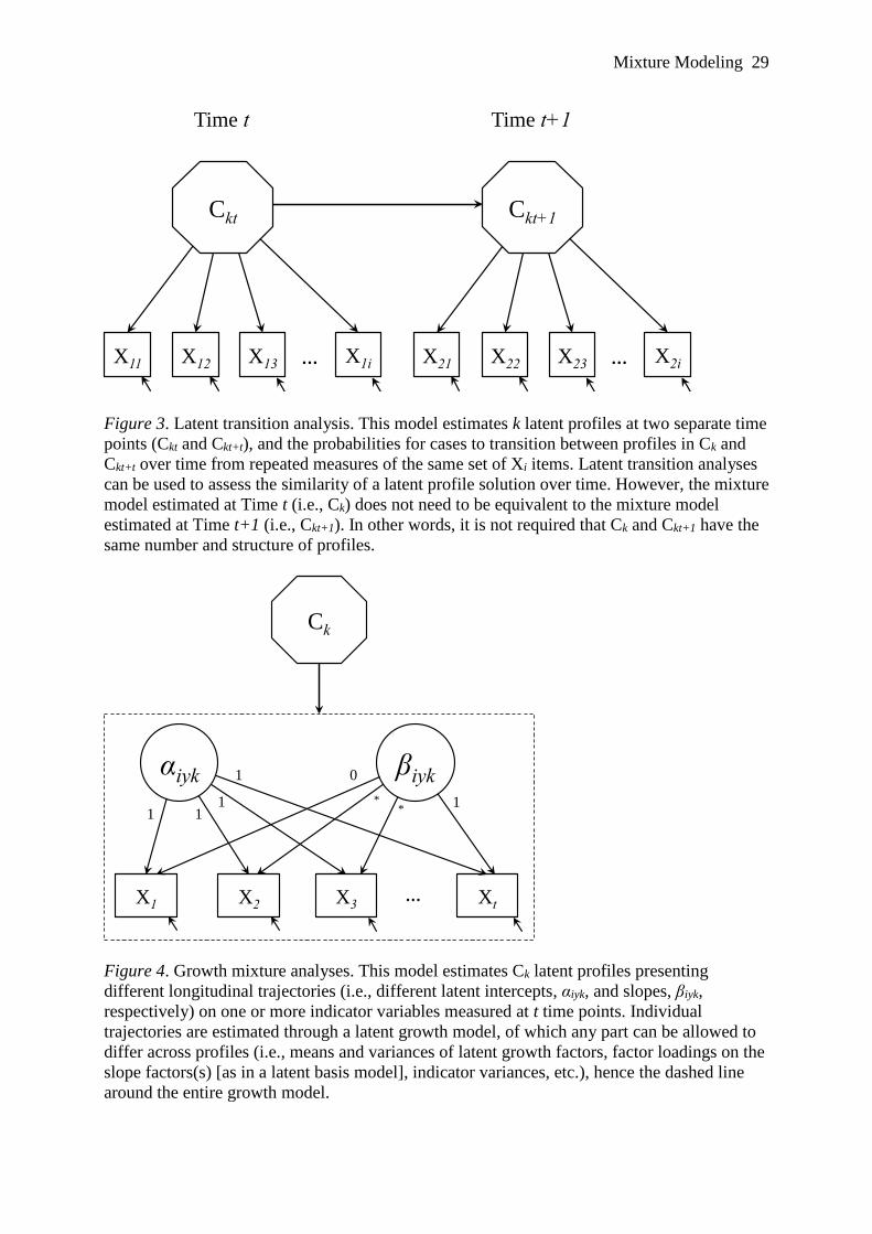
Mixture Modeling 29
Figure 3. Latent transition analysis. This model estimates k latent profiles at two separate time
points (Ckt and Ckt+t), and the probabilities for cases to transition between profiles in Ck and
Ckt+t over time from repeated measures of the same set of Xi items. Latent transition analyses
can be used to assess the similarity of a latent profile solution over time. However, the mixture
model estimated at Time t (i.e., Ck) does not need to be equivalent to the mixture model
estimated at Time t+1 (i.e., Ckt+1). In other words, it is not required that Ck and Ckt+1 have the
same number and structure of profiles.
X11 …X12 X13 X1i
Ckt
X21 …X22 X23 X2i
Ckt+1
Time t Time t+1
Figure 4. Growth mixture analyses. This model estimates Ck latent profiles presenting
different longitudinal trajectories (i.e., different latent intercepts, αiyk, and slopes, βiyk,
respectively) on one or more indicator variables measured at t time points. Individual
trajectories are estimated through a latent growth model, of which any part can be allowed to
differ across profiles (i.e., means and variances of latent growth factors, factor loadings on the
slope factors(s) [as in a latent basis model], indicator variances, etc.), hence the dashed line
around the entire growth model.
X1 X2 X3 Xt
Ck
…
αiyk βiyk
1 1
1
1 0
1 *
*

Mixture Modeling 30
Table 1. Tests of Profile Similarity
Test Description
A – Configural Similarity • Assesses whether same number of profile s are identified in all groups or at each time point. • Configural similarity is a prerequisite to all further similarity tests. • Lacking configural similarity suggests that the latent profile solutions and require a qualitative comparison process.
B – Structural Similarity • Assesses whether within-profile levels on the indicators are the same in all groups/time points (i.e., whether profile structure is similar). • Configural and structural similarity are prerequisite to all further tests, but partial str uctural similarity is possible. • Lack of partial structural similarity: The profiles differ across groups and require a qualitative comparison process. • Prerequisite: Configural similarity.
C – Dispersional Similarity • Assesses whether levels of within -profile variability are the same in all groups/time points. Partial dispersion similarity is possible. • Lack of dispersion similarity: The inter-individual differences among profile members changes across groups /time points. • Not applicable when profile indicators are categorical. • Prerequisite: Configural and structural similarity.
D – Distributional Similarity • Assesses whether the relative size of the profiles (i.e., proportion of sample assigned to each profile) is the same in all groups/ time points. • The size of all profiles needs to be either similar or not across pairs of groups/time points, but partial distributional similarity is possible
across different pairs (e.g., Group 1 and be similar to Group 2, but different than Group 3). • Lack of distributional similarity: The size of the profiles differs across groups. • Prerequisite: Configural and structural similarity.
E – Predictive Similarity • Assesses whether the effects of predictors on profile membership are the same in all groups. • Predictors are directly included into the most similar model (Models A-D, above). • Effects of any one predictor can be similar or not across pairs of profiles, but partial predictive similarity is possible across different pairs
of groups, or across different predictors. • Lack of predictive similarity: The effects of predictors on profile membership differ across groups. • Prerequisite: Configural and structural similarity.
F – Explanatory Similarity • Assesses whether the effects of profile membership on outcome levels are the same in all groups/time points. • Outcomes are directly included into the most similar model (Models A-D, above). • Partial explanatory similarity is possible. • Lack of explanatory similarity: The effects of profile membership on the outcomes differ across groups. • Prerequisite: Configural and structural similarity.
G – Regression Similarity • Assesses whether the regressions that define mixture regression profil es are the same in all groups/time points. • Only relevant in mixture regression analyses, and is the second step of similarity analyses for mixture regression models. • Partial similarity is possible. • Lack of partial regression similarity: The latent profiles differ across groups and require a qualitative comparison process . • Prerequisite: Configural similarity.
Recommended order Steps that are a prerequisite to subsequent steps are bolded.
Latent Profile Analyses: A-B-C-D-E-F
Mixture Regression Analyses: A-G-B-C-D-E-F

Supplements for Mixture Modeling S1
Online Supplemental Material for:
Chapter X. Mixture Modeling in Organizational Behavior Research
Alexandre J.S. Morin*
Substantive-Methodological Synergy Research Laboratory
Department of Psychology, Concordia University
Matthew J. W. McLarnon*
Department of Psychology, Oakland University
David Litalien
Département des fondements et pratiques en éducation
Faculté des sciences de l'éducation, Université Laval
* The first two authors (AJSM & MJWM) contributed equally to this chapter and both should
be considered first authors.

Supplements for Mixture Modeling S2
Appendix A
Technical Considerations in the Estimation of Mixture Models
Mixture Indicators
Most commonly mixture models are estimated on the basis of either continuous or
categorical observed data, though other types of data such as count or nominal variables can
also be used. When categorical data (i.e., binary or polytomous items) is used, the term latent
class analysis (LCA) is often used to describe the mixture model. In LCA, the distinct
subpopulations recovered differ on the basis of item response probabilities (e.g., McLarnon,
DeLongchamp, & Schneider, 2019; Wang & Wang, 2012). Latent profile analysis (LPAs), on
the other hand, are most often estimated using scale scores on the various indicators of interest
(i.e., taking the average of the items used to assess a focal construct and using those scores as
input data; see McLarnon, Carswell, & Schneider, 2015; O’Neill, McLarnon, Hoffart, Woodley,
& Allen, 2018; O’Neill, McLarnon, Xiu, & Law, 2016; or by using factor scores exported from
preliminary measurement models, see below). Throughout, we retain use of LPA given that the
LCA-LPA distinction is somewhat subtle, and that categorical, ordinal, and continuous
indicator variables can be included in the same mixture model (i.e., as a form of hybrid model;
see Berlin, Williams, & Parra, 2014; Muthén & Muthén, 2017).
This supplemental material provides an overview of a number of nuanced issues
associated with thoroughly conducting LPA, and is structured in the following way: first, we
highlight the use of factor scores as the input variables for a LPA. Second, we discuss the
technical issues of random starts in LPA. Third, we present a number of potential guidelines
that researchers may be able to use to make decisions on model fit (i.e., profile or class
enumeration). Finally, we provide a number of detailed Mplus syntax templates that researchers
may be able to leverage to conduct LPAs and its variants.
Although using observed scale scores as input to a LPA is common, there is an important
limitation in doing so: scale scores generally have less-than-perfect reliability, and may
therefore be impacted by measurement error. In contrast, a latent variable (stemming from a
factor analytic model) naturally controls for measurement error (e.g., Bollen, 1989).
Unfortunately, applications of fully latent mixture models in which the means of latent factors
(specified within a confirmatory factor model) vary across profiles are few (see however Morin,
Scalas, & Marsh, 2015). This can, in part, be explained by the complexity of mixture models,
which may make fully latent approaches computationally intractable with common computer
hardware due to nonconvergence or convergence upon improper solutions.
A strategy that reaches a compromise between these issues is to instead rely on factor
scores saved from preliminary measurement models (e.g., Kam, Morin, Meyer, & Topolnytsky,
2015; Morin & Marsh, 2015). Although factors scores do not explicitly control for measurement
errors with equal efficacy as latent variables, they can provide a partial implicit control for
measurement errors by giving differentially more weight to the more reliable items (i.e., those
items with stronger factor loadings). As such, they provide researchers with a reasonable
alternative to the use of observed scale scores. In addition, factors scores tend to preserve the
nature of the underlying measurement structure in a superior manner compared to scale scores
(e.g., can provide methodological controls, account for a bifactor solution or cross-loadings;
Morin, Boudrias et al., 2016, 2017). Notably, the measurement structure of a multidimensional
instrument may not be as clear as a set of observed scale scores would reflect. More specifically,
the simple structure of a multidimensional inventory should be verified prior to using the focal
variables in a mixture model. This verification may potentially lead to investigating the
psychometric structure of an inventory with exploratory structural equation modeling and/or
bifactor exploratory structural equation modeling (Marsh, Morin, Parker, & Kaur, 2014; Marsh,
Nagengast, & Morin, 2013; McLarnon & Tarraf, 2017; Taku & McLarnon, 2018). Without
accounting for an inventory’s complex measurement structure, a resulting profile solution may

Supplements for Mixture Modeling S3
not accurately represent the underlying phenomenon and classification of interest, and may
therefore have questionable construct validity. A third advantage of factor scores, which might
tend to be crucially important in cross-cultural and/or longitudinal research, is that preliminary
measurement models can be used to systematically assess the invariance of a measure across
groups and/or time points (Millsap, 2011). In these research designs, factor scores can be saved
from the most invariant measurement model, ensuring comparability across groups and/or time
points. A final advantage of factors scores comes from their natural standardization, making
them directly and easily interpretable with a mean of zero and a variance of one.
Random Starts
Mixture models are estimated through an iterative process that risks converging on a
local solution, rather than on a true maximum likelihood, when the number of starting values is
not sufficient (Hipp & Bauer, 2006). Therefore, best practice is to estimate mixture models
using many sets of random starting values, and allowing each set of starting values to iterate
sufficiently (Hipp & Bauer, 2006; McLachlan & Peel, 2000). Despite a general recognition that
‘the more, the better’ applies to sets of random starting values, increasing the number of random
starts also increases the computation time for each model under investigation. In practice, our
recommendation is to use at least 3000 sets of random starting values, allowing up to 100
iterations for each of these sets, and retaining the 100 best sets of starting values (i.e., those that
have resulted in the highest loglikelihood estimates) for a final stage of optimizations. The
Mplus syntax requesting these specifications is given below, as these recommendations
override the Mplus defaults. These values can be increased to 5000, 200, and 200, respectively,
when the final solution is not sufficiently replicated. Moreover, we see these values as
minimums that can be increased as needed. We often use even larger values in our own research
(e.g., 10000; 1000; 500; respectively).
For interested readers, Masyn (2013) presented an introduction to maximum likelihood
estimation and the use of an expectation-maximization algorithm in mixture modeling.
Class Enumeration
Alternative profile solutions that extract differing numbers of latent profiles (often
ranging from one profile to the number of profiles that exceeds theoretical expectations, though
rarely greater than 10 profiles) are typically contrasted in order to select the final, optimal
solution. Selection of the optimal model is determined on the basis of considering (a) the
substantive meaning and theoretical conformity of the solution, (b) the statistical adequacy of
the solution, and (c) the statistical indicators and model fit indices accompanying each solution.
Focusing on the statistical indicators of model-data fit: the Akaike Information Criterion
(AIC), the Consistent AIC (CAIC), the Bayesian information criterion (BIC), and the sample-
adjusted BIC (SABIC) are often reported as components of a comprehensive assessment of a
profile solution’s fit. Although the CAIC is not currently provided by Mplus, it can be easily
calculated as BIC + fp, where fp is the number of free parameters. These information criteria
are considered in terms of ‘lower is better,’ such that lower values indicate a better-fitting
model. Traditional likelihood ratio tests (LRT) are inappropriate for profile enumeration
purposes to compare, for instance, the loglikelihood values across models with two versus three
profiles (LRTs can be appropriate for the comparisons of nested models based on the same
variables and number of profiles, as in several of the models presented later in this supplemental
material). For profile enumeration, alternative LRT approximations are available: the Lo,
Mendel and Rubin (2001) LRT (the standard [LMR] and adjusted version of this test [ALMR],
which typically yield the same conclusions), and the bootstrapped LRT (BLRT; McLachlan &
Peel, 2000). These LRT variations compare a k-profile model with a k-1-profile model. BLRT
p-values > .05 indicate that the k-1 profile model should be retained over a k-profile model (see
Nylund, Asparouhov, & Muthén, 2007). Finally, although it should not be used for enumeration
purposes, the entropy estimate associated with each model provides a summary of classification

Supplements for Mixture Modeling S4
accuracy, with larger values (closer to 1) indicating greater accuracy.
Multiple simulation studies (for a recent review, see Diallo, Morin, & Lu, 2016) indicate
that four of these indicators (the CAIC, BIC, ABIC, and BLRT) are particularly effective, while
less emphasis should be placed on the AIC and LMR/ALMR (Diallo, Morin, & Lu, 2016, 2017;
Henson et al., 2007; McLachlan & Peel, 2000; Nylund et al., 2007; Peugh & Fan, 2013, 2014;
Tein, Coxe, & Cham, 2013; Tofighi & Enders, 2008; Tolvanen, 2007; Yang, 2006). When these
indicators fail to retain the optimal model by indicating which model reaches a minimum on
the information criteria, the BIC and CAIC tend to underestimate the true number of profiles,
and the AIC, ABIC, and BLRT tend to overestimate it. The simulation study of Diallo, Morin,
and Lu (2017) further suggested that the BIC and CAIC should be privileged under conditions
of high entropy (≥ .80), whereas the ABIC and BLRT perform better in conditions of low
entropy (≤ .60). However, all of these indicators can also be heavily influenced by sample size
(Marsh, Lüdtke, Trautwein, & Morin, 2009), which means that with sufficiently large samples,
they may suggest a need for additional of profiles to reach adequate fit without ever converging
on a solution that demonstrates the lowest values on these indices. When this happens, it is
recommended to rely on an “elbow plot” (Morin, Maïano, et al., 2011; Petras & Masyn, 2010).
These plots illustrate the gains in fit (i.e., decreasing values of the information criteria) related
to each additional profile. The point after which the slope flattens suggests the optimal number
of profiles. Examples of using elbow plots to inform judgments of profile enumeration can be
found in Chen, Morin, Parker, and Marsh (2015), Ciarrochi, Morin, Sahdra, Litalien, and Parker
(2017), Litalien, Morin, and McInerney (2017), McLarnon and O’Neill (2018), McLarnon et
al. (2019), and Meyer, Morin, Stanley, and Maltin (2019), among others.

Supplements for Mixture Modeling S5
References
Asparouhov, T., & Muthén, B.O. (2012). Using Mplus TECH11 and TECH14 to test the
number of latent classes (Mplus Web Note #14). Retrieved from
http://statmodel.com/examples/webnotes/webnote14.pdf
Asparouhov, T. & Muthén, B.O. (2014). Auxiliary variables in mixture modeling: Three-step
approaches using Mplus. Structural Equation Modeling, 21, 329-341.
doi:10.1080/10705511.2014.915181
Asparouhov, T., & Muthén, B.O. (2015). Auxiliary variables in mixture modeling: Using the
BCH method in Mplus to estimate a distal outcome model and an arbitrary secondary
model (Mplus Web Note #21). Retrieved from
https://www.statmodel.com/download/asparouhov_muthen_2014.pdf
Bakk, Z., & Kuha, J. (2018). Two-step estimation of models between latent classes and external
variables. Psychometrika, 83, 871-892. doi:10.1007/s11336-017-9592-7
Bakk, Z., & Vermunt, J.K. (2016). Robustness of stepwise latent class modeling with
continuous distal outcomes. Structural Equation Modeling, 23, 20-31.
doi:10.1080/10705511.2014.955104
Berlin, K.S., Williams, N.A., & Parra, G.R. (2014). An introduction to latent variable mixture
modeling (Part 1): Cross sectional latent class and latent profile analyses. Journal of
Pediatric Psychology, 39, 174-187. doi:10.1093/jpepsy/jst084
Bollen, K.A. (1989). Structural equations with latent variables. New York, NY: Wiley.
Chénard Poirier, L.-A., Morin, A.J.S., & Boudrias, J.-S.(2017). On the merits of coherent
leadership empowerment behaviors: A mixture regression approach. Journal of
Vocational Behavior, 103, 66-75. doi:10.1016/j.jvb.2017.08.003
Chen, X., Morin, A.J.S., Parker, P.D., & Marsh, H.W. (2015). Developmental investigation of
the domain-specific nature of the life satisfaction construct across the post-school
transition. Developmental Psychology, 51, 1074-1085. doi:10.1037/a0039477
Ciarrochi, J., Morin, A.J.S., Sahdra, B.K., Litalien, D., & Parker, P.D. (2017). A longitudinal
person-centered perspective on youth social support: Relations with psychological
wellbeing. Developmental Psychology, 53, 1154-1169. doi:10.1037/dev0000315
Diallo, T.M.O, Morin, A.J.S., & Lu, H. (2016). Impact of misspecifications of the latent
variance-covariance and residual matrices on the class enumeration accuracy of growth
mixture models. Structural Equation Modeling, 23, 507-531.
doi:10.1080/10705511.2016.1169188
Diallo, T.M.O., Morin, A.J.S., & Lu, H. (2017). The impact of total and partial inclusion or
exclusion of active and inactive time invariant covariates in growth mixture models.
Psychological Methods, 22, 166-190. doi:10.1037/met0000084
Eid, M., Langeheine, R., & Diener, E. (2003). Comparing typological structures across cultures
by multigroup latent class analysis: A primer. Journal of Cross-Cultural Psychology,
34, 195-210. doi:10.1177/0022022102250427
Geiser, C., Lehmann, W., & Eid, M. (2006). Separating “rotators” from “nonrotators” in the
Mental Rotations Test: A multigroup latent class analysis. Multivariate Behavioral
Research, 41, 261-293. doi:10.1207/s15327906mbr4103_2
Henson, J.M., Reise, S.P., & Kim, K.H. (2007). Detecting mixtures from structural model
differences using latent variable mixture modeling: A comparison of relative model fit
statistics. Structural Equation Modeling, 14, 202-226.
doi:10.1080/10705510709336744
Hipp, J.R., & Bauer, D.J. (2006). Local solutions in the estimation of growth mixture
models. Psychological Methods, 11, 36-53. doi:10.1037/1082-989X.11.1.36
Janssen, J.H.M., van Laar, S., de Rooij, M.J., Kuha, J., & Bakk, Z. (in press). The detection and
modeling of direct effects in latent class analysis. Structural Equation Modeling.

Supplements for Mixture Modeling S6
doi:10.1080/10705511.2018.1541745
Kam, C., Morin, A.J.S., Meyer, J.P., & Topolnytsky, L. (2016). Are commitment profiles stable
and predictable? A latent transition analysis. Journal of Management, 42, 1462-1490.
doi:10.1177/0149206313503010
Kankaraš, M., Moors, G., & Vermunt, J.K. (2011). Testing for measurement invariance with
latent class analysis. In E. Davidov, P. Schmidt & J. Billiet (Eds.), Cross-cultural
analysis: Methods and applications (pp. 359-384). New York, NY: Routledge.
Landis, R.S., Edwards, B.D., & Cortina, J.M. (2009). On the practice of allowing correlated
residuals among indicators in structural equation models. In. C.E. Lance & R.J.
Vandenberg (Eds.), Statistical and methodological myths and urban legends (pp. 37-
59). New York: Routledge.
Lanza, S.T., Tan, X., & Bray, B.C. (2013). Latent class analysis with distal outcomes: A flexible
model-based approach. Structural Equation Modeling, 20, 1-26.
doi:10.1080/10705511.2013.742377
Litalien, D., Morin, A.J.S., & McInerney, D.M. (2017). Achievement goal profiles among
adolescent males and females. Developmental Psychology, 53, 731-751.
doi:10.1037/dev0000288
Lo, Y., Mendell, N., & Rubin, D. (2001). Testing the number of components in a normal
mixture. Biometrika, 88, 767-778. doi:10.1093/biomet/88.3.767
Marsh, H.W., Hau, K.-T., & Grayson, D. (2005). Goodness of fit evaluation in structural
equation modeling. In A. Maydeu-Olivares, & J. McArdle (Eds.), Contemporary
psychometrics (pp. 275-340). Hillsdale, NJ: Erlbaum.
Marsh, H.W., Lüdtke, O., Trautwein, U., & Morin, A.J.S. (2009). Classical latent profile
analysis of academic self-concept dimensions: Synergy of person- and variable-centered
approaches to theoretical models of self-concept. Structural Equation Modeling, 16,
191-225. doi:10.1080/10705510902751010
Marsh, H.W., Morin, A.J.S., Parker, P., & Kaur, G. (2014). Exploratory structural equation
modeling: An integration of the best features of exploratory and confirmatory factor
analysis. Annual Review of Clinical Psychology, 10, 85-110. doi:10.1146/annurev-
clinpsy-032813-153700
Marsh, H.W., Nagengast, B., & Morin, A.J.S. (2013). Measurement invariance of big-five
factors over the life span: ESEM tests of gender, age, plasticity, maturity, and la dolce
vita effects. Developmental Psychology, 49, 1194-1218. doi:10.1037/a0026913
Masyn, K. (2013). Latent class analysis and finite mixture modeling. In T.D. Little (Ed.), The
Oxford handbook of quantitative methods in psychology (Vol. 2, pp. 551-611). New
York: Oxford University Press.
McLachlan, G.J., & Peel, D. (2000). Finite mixture models. New York, NY: Wiley.
McLarnon, M.J.W., Carswell, J.J., & Schneider, T.J. (2015). A case of mistaken identity?
Latent profiles in vocational interests. Journal of Career Assessment, 23, 166-185.
doi:10.1177/1069072714523251
McLarnon, M.J.W., DeLongchamp, A.C., & Schneider, T.J. (2019). Faking it! Individual
differences in types and degrees of faking behavior. Personality and Individual
Differences, 138, 88-95. doi:10.1016/j.paid.2018.09.024
McLarnon, M.J.W., & O’Neill, T.A. (2018). Extensions of auxiliary variable approaches for
the investigation of mediation, moderation, and conditional effects in mixture models.
Organizational Research Methods, 21, 955-982. doi:10.1177/1094428118770731
McLarnon, M.J.W., & Tarraf, R.C. (2017). The Dark Triad: Specific or general sources of
variance? A bifactor exploratory structural equation modeling approach. Personality
and Individual Differences, 112, 67-73. doi:10.1016/j.paid.2017.02.049
McNeish, D., Stapleton, L.M., & Silverman, R. D. (2017). On the unnecessary ubiquity of

Supplements for Mixture Modeling S7
hierarchical linear modeling. Psychological Methods, 22, 114-140.
doi:10.1037/met0000078
Mehta, P.D., & West, S.G. (2000). Putting the individual back into individual growth curves.
Psychological Methods, 5, 23-43. doi:10.1037/1082-989X.5.1.23
Meyer, J.P., Morin, A.J.S., Stanley, L.J., & Maltin, E.R. (2019). Teachers’ dual commitment to
the organization and occupation: A person-centered investigation. Teaching and
Teacher Education, 77, 100-111. doi:10.1016/j.tate.2018.09.009
Millsap, R.E. (2011). Statistical approaches to measurement invariance. New York: Routledge.
Morin, A.J.S., Boudrias, J.-S., Marsh, H.W., McInerney, D.M., Dagenais-Desmarais, V.,
Madore, I., & Litalien, D. (2017). Complementary variable- and person-centered
approaches to exploring the dimensionality of psychometric constructs: Application to
psychological wellbeing at work. Journal of Business and Psychology, 32, 395-419.
doi:10.1007/s10869-016-9448-7
Morin, A.J.S., Boudrias, J.-S., Marsh, H.W., Madore, I., & Desrumaux, P. (2016). Further
reflections on disentangling shape and level effects in person-centered analyses: An
illustration aimed at exploring the dimensionality of psychological health. Structural
Equation Modeling, 23, 438-454. doi:10.1080/10705511.2015.1116077
Morin, A.J.S., & Litalien, D. (2017). Webnote: Longitudinal tests of profile similarity and latent
transition analyses. Retrieved January 5, 2019 from
https://smslabstats.weebly.com/uploads/1/0/0/6/100647486/lta_distributional_similarity_v
02.pdf. Montreal, QC: Substantive Methodological Synergy Research Laboratory.
Morin, A.J.S., Maïano, C., Nagengast, B., Marsh, H.W., Morizot, J., & Janosz, M. (2011).
General growth mixture analysis of adolescents’ developmental trajectories of anxiety:
The impact of untested invariance assumptions on substantive interpretations.
Structural Equation Modeling, 18, 613-648. doi:10.1080/10705511.2011.607714
Morin, A.J.S., & Marsh, H.W. (2015). Disentangling shape from level effects in person-
centered analyses: An illustration based on university teachers’ multidimensional
profiles of effectiveness. Structural Equation Modeling, 22, 39-59.
doi:10.1080/10705511.2014.919825
Morin, A.J.S., Meyer, J.P., Creusier, J., & Biétry, F. (2016). Multiple-group analysis of
similarity in latent profile solutions. Organizational Research Methods, 19, 231-254.
doi:10.1177/1094428115621148
Morin, A.J.S., Morizot, J., Boudrias, J.-S., & Madore, I., (2011). A multifoci person-centered
perspective on workplace affective commitment: A latent profile/factor mixture
analysis. Organizational Research Methods, 14, 58-90.
doi:10.1177/1094428109356476
Morin, A.J.S., Scalas, L.F., & Marsh, H.W. (2015). Tracking the elusive actual-ideal
discrepancy model within latent subpopulations. Journal of Individual Differences, 36,
65-72. doi:10.1027/1614-0001/a000157
Muthén, B.O., & Satorra, A. (1995). Complex sample data in structural equation modeling.
Sociological Methodology, 25, 267-316. doi:10.2307/271070
Muthén, L.K., & Muthén, B.O. (2017). Mplus User’s Guide (8th ed.). Los Angeles: Muthén &
Muthén.
Nylund, K.L., Asparouhov, T., & Muthén, B.O. (2007). Deciding on the number of classes in
latent class analysis and growth mixture modeling: A Monte Carlo simulation study.
Structural Equation Modeling, 14, 535-569. doi:10.1080/10705510701575396
Nylund-Gibson, K.L., Grimm, R., Quirk, M., & Furlong, M. (2014). A latent transition mixture
model using the three-step specification. Structural Equation Modeling, 21, 439-454.
doi:10.1080/10705511.2014.915375
O’Neill, T.A., McLarnon, M.J.W., Hoffart, G.C., Woodley, H.J., & Allen, N.J. (2018). The

Supplements for Mixture Modeling S8
structure and function of team conflict state profiles. Journal of Management, 44, 811-
836. doi:10.1177/0149206315581662
O’Neill, T.A., McLarnon, M.J.W., Xiu, L., & Law, S.J. (2016). Core self-evaluations,
perceptions of group potency, and job performance: The moderating role of
individualism and collectivism cultural profiles. Journal of Occupational and
Organizational Psychology, 89, 447-473. doi:10.1111/joop.12135
Pastor, D.A., Barron, K.E., Miller, B.J., & Davis, S.L. (2007). A latent profile analysis of
college students’ achievement goal orientation. Contemporary Educational Psychology,
32, 8-47. doi:10.1016/j.cedpsych.2006.10.003
Petras, H., & Masyn, K. (2010). General growth mixture analysis with antecedents and
consequences of change. In A.R. Piquero, & D. Weisburd (Eds.), Handbook of
quantitative criminology (pp. 69-100). New York: Springer.
Peugh, J., & Fan, X. (2013). Modeling unobserved heterogeneity using latent profile analysis:
A Monte Carlo simulation. Structural Equation Modeling, 20, 616-639.
doi:10.1080/10705511.2013.824780
Peugh, J., & Fan, X. (2014). Enumeration index performance in generalized growth mixture
models: A Monte Carlo test of Muthén’s (2003) hypothesis. Structural Equation
Modeling, 23, 115-131. doi:10.1080/10705511.2014.919823
Raykov, T., & Marcoulides, G.A. (2004). Using the delta method for approximate interval
estimation of parameter functions in SEM. Structural Equation Modeling, 11, 621-637.
doi:10.1207/s15328007sem1104_7
Taku, K., & McLarnon, M.J.W. (2018). Posttraumatic growth profiles and their relationships
with HEXACO personality traits. Personality and Individual Differences, 134, 33-42.
doi:10.1016/j.paid.2018.05.038
Tein, J.-Y., Coxe, S., & Cham, H. (2013). Statistical power to detect the correct number of
classes in latent profile analysis. Structural Equation Modeling, 20, 640-657.
doi:10.1080/10705511.2013.824781
Tofighi, D., & Enders, C. (2008). Identifying the correct number of classes in growth mixture
models. In G.R. Hancock & K.M. Samuelsen (Eds.), Advances in latent variable
mixture models (pp. 317-341). Charlotte, NC: Information Age.
Tolvanen, A. (2007). Latent growth mixture modeling: A simulation study. PhD dissertation,
Department of Mathematics, University of Jyväskylä, Jyväskylä, Finland.
Vermunt, J.K. (2010). Latent class modeling with covariates: Two improved three-step
approaches. Political Analysis, 18, 450-469. doi:10.1093/pan/mpq025
Wang, J., & Wang, X. (2012). Structural equation modeling: Applications using Mplus. West
Sussex, UK: John Wiley & Sons.
Yang, C. (2006). Evaluating latent class analyses in qualitative phenotype identification.
Computational Statistics & Data Analysis, 50, 1090-1104. doi:10.1016/j.csda.2004.11.004

Supplements for Mixture Modeling S9
Appendix B
Mplus Syntax for the Estimation of Mixture Models
In Mplus syntax, annotations can be preceded by an exclamation mark, !, and are not interpreted
by the program. All Mplus commands are not case sensitive.
DATA
The first part of the Mplus syntax identifies the dataset to be used in the analysis. If the dataset
is in the same folder as the input file (the recommended strategy), only the filename of the
dataset needs to be indicated. If the dataset is in another folder then the full path needs to be
specified. Here, the dataset, saved as a comma-separated values file (*.csv; but we also
frequently use tab-delimited *.dat files) that can be opened and manipulated in Microsoft Excel
or other standard spreadsheet software, is labeled “filename.csv” and is located in the same
folder as the Mplus input file (i.e., the *.inp file containing the syntax).
TITLE: Mixture Modeling in Organizational Behavior Research
!A title is not a required syntax component, but can be helpful to track files and results
DATA:
FILE IS ‘filename.csv’;
VARIABLE
In the VARIABLE section of the syntax, the NAMES function identifies all variables included
in the dataset, in order of appearance. USEVARIABLES specifies the variables to be used in
the analysis. Here, only the variables IND1_T1, IND2_T1, and IND3_T1 are being considered
as indicators of a latent profile (IND is used as a generic label for “indicator”; 1, 2, and 3
represents the i set of indicators; and _T1 reflects Time 1 measures). Variable names should be
restricted to eight characters or less. MISSING defines the values in each variable that denote
a missing piece of data (typically the same value is used for all variables). Here, any instance
of “999” would be interpreted by Mplus as a missing value. The IDVARIABLE function
defines the unique identifier for each case (i.e., participant, employee, team, etc.). CLASSES
defines the number of latent profiles estimated (here, 3), with the “C” preceding the number in
parentheses being an arbitrary label assigned to the latent categorical variable that defines the
latent profiles to be extracted. As noted, most typically, multiple LPAs are conducted, in a
somewhat exploratory approach, by varying the number of profiles extracted, so in other
analyses models with 1, 2, 4, 5, etc. profiles would also be specified.
USEOBSERVATIONS can be used to limit the estimation to a subset of cases. In this
example, if the ! is removed, the function would limit the estimation to women (identified by
the Gender variable, which might have the coding of 1 = males; 2 = females) and would exclude
men and cases with missing gender information. The CLUSTER function can be used to define
a unique identifier for a clustering variable (i.e., a level-2 variable) to be controlled for or
accounted for in the analysis (e.g., teams, classrooms, etc.), or to enable multilevel
specifications. By default, Mplus considers variables as continuous. However Mplus can
accommodate categorical (binary or polytomous), censored, count, or nominal variables (see
Muthén & Muthén, 2017). The appropriate variables would just be specified by each of these
respective commands (and the exclamation point removed) to be incorporated into an analysis.
Notably, the NOMINAL specification will be used later in this material to illustrate the manual
implementation of the three-step procedure used to investigate covariate relations.

Supplements for Mixture Modeling S10
VARIABLE:
NAMES = ID Gender Team_ID Pred1 Pred2 Cor1 Cor2 Out1 Out2
IND1_T1 IND2_T1 IND3_T1
IND1_T2 IND2_T2 IND3_T2;
USEVARIABLES = IND1_T1 IND2_T1 IND3_T1;
! CATEGORICAL = ;
! CENSORED = ;
! COUNT = ;
! NOMINAL = ;
MISSING = all (999);
IDVARIABLE = ID;
CLASSES = C(3);
CLUSTER = Team_ID;
! USEOBSERVATIONS Gender EQ 2;
ANALYSIS:
The ANALYSIS section describes the technical specifications of the LPA itself. Here, we
request the estimation of a mixture model (TYPE = MIXTURE;), which includes a correction
for the nesting of cases within a higher-level unit (i.e., work team; TYPE = COMPLEX;).
Further, we request that Mplus uses its robust maximum likelihood estimator (ESTIMATOR =
MLR;), which provides standard errors that are robust to non-normality, and to non-
independence when used in conjunction with TYPE=COMPLEX; (McNeish, Stapleton, &
Silverman, 2017; Muthén & Satorra, 1995; Muthén & Muthén, 2017; Mplus uses MLR by
default for mixture models so it is not necessary to declare this explicitly). STARTS = 3000
100; requests 3000 initial sets of random start values, with the best 100 of these starts (i.e., those
that result in the highest loglikelihood values; see below) being retained for a final set of
optimization iterations. STITERATIONS = 100; requests that all random starts be allowed a
maximum of 100 iterations. PROCESS = 3; requests that 3 of the available processors in the
local computer be used to speed up the estimation (i.e., 1/3 of the random starts will be allocated
to each processor to distribute the model estimation and complete it in parallel).
ANALYSIS:
TYPE = MIXTURE COMPLEX;
ESTIMATOR = MLR;
PROCESS = 3;
STARTS = 3000 100;
STITERATIONS = 100;
As part of the output, Mplus provides the loglikelihood values associated with each of the
random starting value runs that were retained for the final stage of optimization iterations and
reached convergence. The output will also indicate how many of the start value runs did not
converge (i.e., the “perturbed” values, in this example there are 15 [of 100] that did not reach
convergence). The first number in this list gives the loglikelihood value (-6095.887), the second
number (991399) is the random seed value that resulted in this loglikelihood, and the third
number (1433) is the ordering within the 3000 random starting value sets that resulted in this
random seed and associated loglikelihood.

Supplements for Mixture Modeling S11
RANDOM STARTS RESULTS RANKED FROM THE BEST TO THE WORST
LOGLIKELIHOOD VALUES
15 perturbed starting value run(s) did not converge.
Final stage loglikelihood values at local maxima, seeds, and initial stage start numbers:
-6095.887 991399 1433
-6095.887 165268 2436
-6095.887 551639 55
-6095.887 58353 1723
-6095.887 168648 1788
-6095.887 445692 2796
-6095.887 973369 202
-6095.887 623887 2611
-6096.828 163110 584
-6096.828 762461 425
-6096.828 62715 2599
-6104.647 264951 1130
-6104.647 930872 277
-6104.647 670998 1876
-6104.698 98068 998
-6105.491 361131 2563
…
In this example, the best loglikelihood value was replicated eight times (in bold; the number of
times the value of -6095.887 appears in the first column), which is satisfactory. Although no
clear-cut rule exists, we suggest that solutions should be replicated at least three times.
Otherwise, the results may not be robust, and these loglikelihood values could reflect a local
solution, rather than a global optimum. Should a model fail to sufficiently replicate the best
loglikelihood, additional tests should be conducted with an increased number of random starting
value sets and/or iterations (e.g., STARTS = 10000 1000; STITERATIONS = 1000;), or by
using user-defined start values. Alternatively, the values from the best fitting, non-replicated
solution, which are provided when SVALUES is requested in the OUTPUT section of the
syntax (see below) can be copied into the MODEL portion of the syntax while keeping the
random starts function active (we provide an example below). As noted, the second column
provides the random seed associated with each random starting value set. Using the seed
number can provide an easy way to replicate the final solution (or any other solution) while
decreasing computational time (i.e., the same loglikelihood value and parameter estimates will
result). To use this procedure, the following ANALYSIS section has been adapted to replicate
the above solution by inputting the seed number into the OPTSEED command. The usage of
the OPTSEED however will not ensure that the solution is replicated if additional variables
(i.e., covariates, predictors, or outcomes) are directly incorporated into the model. We address
this issue in greater detail below.
ANALYSIS:
TYPE = MIXTURE COMPLEX;
ESTIMATOR = MLR;
PROCESS = 3;
STARTS = 0;
OPTSEED = 991399;
STITERATIONS = 100;

Supplements for Mixture Modeling S12
MODEL
The MODEL section of the syntax describes the specific structure of the mixture model to be
estimated. We provide code, in sequence, for each of the models described in the chapter.
OUTPUT
This section of the syntax covers specific output provided by Mplus. Here, we request
standardized model parameters (STDYX), sample statistics (SAMPSTAT), confidence
intervals (CINTERVAL), the final estimates provided by the model that could be used as
starting values for a subsequent analyses (SVALUES), the model residuals (RESIDUAL), the
arrays of parameters (TECH1), the profile-specific descriptives (TECH7), the LMR and ALMR
tests (TECH11), and the BLRT (TECH14). Since the BLRT can be computationally intensive,
users may wish to omit it from an initial set of analyses, and then revisit each solution following
the procedure outlined by Asparouhov and Muthén (2012) to save time with complex models.
OUTPUT:
STDYX SAMPSTAT CINTERVAL SVALUES RESIDUAL TECH1 TECH7 TECH11
TECH14;

Supplements for Mixture Modeling S13
Latent Profile Analysis
The MODEL section includes an %OVERALL% portion that describes the global relations
estimated among the variables that will apply to each profile. Profile-specific statements,
%C#1%, %C#2%, and %C#3% (where C is the arbitrary label used to define the latent
categorical variable from the CLASSES command of the VARIABLE section, and the number
[1 to k] refers to the specific nominal category of this variable [i.e., the specific profile]). Here,
as no commands are presented directly beneath the %OVERALL% section, no relations
between variables will be constrained to equality across profiles (though see later examples and
Pastor, Barron, Miller, & Davis, 2007). As noted, throughout our examples, three profiles are
estimated from three indicators taken at the first time point (IND1_T1, IND2_T1, and
IND3_T1). The profile specific sections request that the means (indicated by the name of the
variable within square brackets [ ]) and variances (defined by the names only) of the indicators
be freely estimated in all profiles.
MODEL:
%OVERALL%
%C#1%
[IND1_T1 IND2_T1 IND3_T1];
IND1_T1 IND2_T1 IND3_T1;
%C#2%
[IND1_T1 IND2_T1 IND3_T1];
IND1_T1 IND2_T1 IND3_T1;
%C#3%
[IND1_T1 IND2_T1 IND3_T1];
IND1_T1 IND2_T1 IND3_T1;
Profiles can also be estimated with the variances of respective indicators held equal across
profiles by removing, or deactivating with !, the profile-specific references of each variable’s
variance:
MODEL:
%OVERALL%
%C#1%
[IND1_T1 IND2_T1 IND3_T1];
%C#2%
[IND1_T1 IND2_T1 IND3_T1];
%C#3%
[IND1_T1 IND2_T1 IND3_T1];

Supplements for Mixture Modeling S14
In Mplus, correlations are identified using a WITH command, so should a researcher wish to
allow correlated uniquenesses among profile indicators, where the correlations are constrained
to equality across profiles, the following could be added to the %OVERALL% section of the
syntax. However, we generally would not recommend this strategy, and would encourage
researchers to use this approach with caution and only with a strong theoretical rationale,
given the well-known issues associated with correlated uniquenesses, which are known to
drastically change the meaning of the estimated latent variables (here the profiles; see Landis,
Edwards, & Cortina, 2009).
MODEL:
%OVERALL%
IND1_T1 WITH IND2_T1 IND3_T1;
IND2_T1 WITH IND3_T1;
%C#1%
[IND1_T1 IND2_T1 IND3_T1];
IND1_T1 IND2_T1 IND3_T1;
%C#2%
[IND1_T1 IND2_T1 IND3_T1];
IND1_T1 IND2_T1 IND3_T1;
%C#3%
[IND1_T1 IND2_T1 IND3_T1];
IND1_T1 IND2_T1 IND3_T1;
To estimate a model with correlated uniquenesses among all profile indicators, which are freely
estimated in all profiles rather than constrained to equality, the following commands can be
adapted. As above, we would not generally recommend this strategy.
MODEL:
%OVERALL%
IND1_T1 WITH IND2_T1 IND3_T1;
IND2_T1 WITH IND3_T1;
! Note, even though the general commands appear here,
! they are ‘over-ridden’ with the profile-specific commands below
%C#1%
[IND1_T1 IND2_T1 IND3_T1];
IND1_T1 IND2_T1 IND3_T1;
IND1_T1 WITH IND2_T1 IND3_T1;
IND2_T1 WITH IND3_T1;
%C#2%
[IND1_T1 IND2_T1 IND3_T1];
IND1_T1 IND2_T1 IND3_T1;
IND1_T1 WITH IND2_T1 IND3_T1;
IND2_T1 WITH IND3_T1;
%C#3%
[IND1_T1 IND2_T1 IND3_T1];
IND1_T1 IND2_T1 IND3_T1;
IND1_T1 WITH IND2_T1 IND3_T1;
IND2_T1 WITH IND3_T1;

Supplements for Mixture Modeling S15
When SVALUES are requested in the output, Mplus will provide a section, similar to the
following. This section can be copy-and-pasted and used as a replacement for the MODEL
section. In conjunction with setting the STARTS command to 0 (STARTS = 0) the final solution
will be replicated without the computational requirements of the random starts. This function
may be particularly useful when including covariates, and may minimize the occurrence of
changes in a LPA following the inclusion of covariates to the model. However, if there is
substantial change (e.g., proportions of cases assigned to each profile, means of indicators in
each profile) between a final unconditional model and a conditional model with covariates, the
researcher should use one of the procedures described below (i.e., the three-step, DCAT, or
BCH approaches; see McLarnon & O’Neill, 2018). Below, we provide an overview of
McLarnon and O’Neill’s (2018) manual approach that can be implemented to incorporate
auxiliary variables when a shift in a profile solution has occurred following the implementation
of direct inclusion approaches.
MODEL: ! COMMANDS WITH FINAL ESTIMATES USED AS STARTING VALUES
%OVERALL%
[ C#1*-0.93515 ];
[ C#2*0.49113 ];
%C#1%
[IND1_T1*-1.59367 ];
[IND2_T1*-0.93155 ];
[IND3_T1*0.39664 ];
IND1_T1*0.53789;
IND2_T1*2.12542;
IND3_T1*1.59137;
%C#2%
[IND1_T1*-0.18248 ];
[IND2_T1*-0.29812 ];
[IND3_T1*-0.15201 ];
IND1_T1*0.42376;
IND2_T1*0.43116;
IND3_T1*0.72513;
%C#3%
[IND1_T1*0.94111 ];
[IND2_T1*0.86526 ];
[IND3_T1*0.08333 ];
IND1_T1*0.44053;
IND2_T1*0.48030;
IND3_T1*1.13489;

Supplements for Mixture Modeling S16
Latent Profile Analysis with Covariates
Predictors
Direct inclusion of predictors into the model is done by way of multinomial logistic regressions
where the predictors are specified as having an impact on profile membership (i.e., C#1-C#2
ON Pred1 Pred2;), where one fewer C# statement than the total number of profiles is necessary
in the %OVERALL% section. The C# portions of the command reflect the multinomial
probability of membership in the various categories of the latent profile variable, which
represent the relative size of each profile and the proportion of the sample assigned to each
profile.
MODEL:
%OVERALL%
C#1-C#2 ON Pred1 Pred2;
%C#1%
[IND1_T1 IND2_T1 IND3_T1];
IND1_T1 IND2_T1 IND3_T1;
%C#2%
[IND1_T1 IND2_T1 IND3_T1];
IND1_T1 IND2_T1 IND3_T1;
%C#3%
[IND1_T1 IND2_T1 IND3_T1];
IND1_T1 IND2_T1 IND3_T1;
To enhance the probability that the nature of the profiles will remain unchanged by the inclusion
of predictors, the SVALUES from the final solution can be used (as noted previously), and the
random starts function should be deactivated (STARTS = 0;). If this is not sufficient to prevent
shifts in the model parameters, the class specific parameters (i.e., variable means and variances
within the %C#1% to %C#3% profile-specific sections) can be fixed (using @ rather than *;
see alternative codes below; see also Bakk & Kuha, 2018; Janssen, van Laar, de Rooij, Kuha,
& Bakk, in press). The start values in the %OVERAL% section to describe that the class
probabilities should not be fixed (i.e., leave these with an asterisk; [C#1*-0.93515 ];), as the
inclusion of predictors changes the meaning of these parameter from reflecting class
probabilities to reflecting the multinomial intercepts of these class probabilities as predicted by
the covariates.
%OVERALL%
[C#1*-0.93515 ]; [C#2*0.49113 ];
C#1-C#2 ON Pred1 Pred2;
%C#1%
[ IND1_T1*-1.59367 ]; ! Alternatively: [ [email protected] ];
[ IND2_T1*-0.93155 ]; ! Alternatively: [ [email protected] ];
[ IND3_T1*0.39664 ]; ! Alternatively: [ [email protected] ];
IND1_T1*0.53789;
IND2_T1*2.12542;
IND3_T1*1.59137;
%C#2%
[IND1_T1*-0.18248 ];
IND2_T1*-0.29812 ];
[IND3_T1*-0.15201 ];
IND1_T1*0.42376;
IND2_T1*0.43116;
IND3_T1*0.72513;

Supplements for Mixture Modeling S17
%C#3%
[IND1_T1*0.94111 ];
[IND2_T1*0.86526 ];
[IND3_T1*0.08333 ];
IND1_T1*0.44053;
IND2_T1*0.48030;
IND3_T1*1.13489;
In contrast to the previous approach in which predictors are directly included into the model,
Mplus also includes a number of approaches that facilitate examining predictor, covariate, and
outcome relations while maintaining these variables as external, or auxiliary, to the focal
mixture model. Advantageously, these approaches preserve the construct validity of an
unconditional profile solution by reducing the likelihood of a shift in the structure and definition
of a profile. In particular, with the direct inclusion approach offered in the previous syntax,
there is a potential for confounding in the meaning and nature of the latent profiles because
covariates can directly contribute information into the estimation of the mixture model. This
means that the profiles could come to reflect the heterogeneity not only in the focal profile
indicators but also in the covariates, potentially raising concerns over the nature of the construct
assessed by the profiles. Accordingly, direct inclusion raises the possibility that a latent profile
“could lose its meaning” (Asparouhov & Muthén, 2014, p. 329). To provide an alternative to
the direct inclusion approach when it results in substantial shifts in the nature of an optimal
unconditional profile solution, Mplus includes a number of auxiliary procedures for examining
relations between a latent profile and covariates without allowing them to influence the nature
of the profiles. In these contexts, covariates are referred to as auxiliary variables. The manual
implementation of these procedures forms the basis of McLarnon and O’Neill’s (2018)
framework for examining auxiliary covariate relations (which is based on Asparouhov &
Muthen, 2014, 2015; Nylund-Gibson, Grimm, Quirk, & Furlong, 2014).
Among the available AUXILIARY approaches automated in Mplus, the R3STEP procedure
(see Asparouhov & Muthén, 2014; Vermunt, 2010) is currently optimal for examining predictor
relations. This approach is similar to the multinomial logistic regressions described above, but
explicitly tests, through an automated procedure, whether including the predictors result in a
change in the nature of the profiles. When this occurs (and the previous direct inclusion
approaches do not work), then predictors should be treated as correlates (see below). To use
R3STEP, the following line of code needs to be included to the VARIABLE section (in bold).
The MODEL section remains unchanged (which can be specified with or without starting
values).
VARIABLE:
NAMES = ID Gender Team_ID Pred1 Pred2 Cor1 Cor2 Out1 Out2
IND1_T1 IND2_T1 IND3_T1
IND1_T2 IND2_T2 IND3_T2;
USEVARIABLES = IND1_T1 IND2_T1 IND3_T1;
MISSING = all (999);
IDVARIABLE = ID;
CLASSES = C(3);
AUXILIARY = Pred1 (R3STEP) Pred2 (R3STEP);

Supplements for Mixture Modeling S18
Outcomes
The direct inclusion of outcomes involves adding them as additional mixture indicators,
preferably while using the SVALUES from the final solution to provide a measure of stability
in the nature of the profiles. Parameter labels are given to the means of the outcome variables
in each profile (in parentheses), and these labels can subsequently be used within a MODEL
CONSTRAINT command to provide tests of significant differences (based on the delta method;
Raykov & Marcoulides, 2004) of the outcome means between profiles. A MODEL TEST
command can also be enabled to provide a Wald χ2 test, as is provided by the automated three-
step and BCH functions.
%OVERALL%
[C#1*-0.93515 ]; [C#2*0.49113 ];
%C#1%
[IND1_T1*-1.59367 ]; [IND2_T1*-0.93155 ]; [IND3_T1*0.39664 ];
IND1_T1*0.53789; IND2_T1*2.12542; IND3_T1*1.59137;
[Out1] (oa1); [Out2] (ob1);
Out1; Out 2;
%C#2%
[IND1_T1*-0.18248 ]; [IND2_T1*-0.29812 ]; [IND3_T1*-0.15201 ];
IND1_T1*0.42376; IND2_T1*0.43116; IND3_T1*0.72513;
[Out1] (oa2); [Out2] (ob2);
Out1; Out 2;
%C#3%
[IND1_T1*0.94111 ]; [IND2_T1*0.86526 ]; [IND3_T1*0.08333 ];
IND1_T1*0.44053; IND2_T1*0.48030; IND3_T1*1.13489;
[Out1] (oa3); Out2] (ob3);
Out1; Out 2;
MODEL CONSTRAINT:
! New parameters are created using this function to reflect pairwise mean differences between
! profiles (e.g., y12 reflects the differences between the Out1 means in profiles 1 and 2) NEW (y12);
y12 = oa1-oa2;
NEW (y13);
y13 = oa1-oa3;
NEW (y23);
y23 = oa2-oa3;
NEW (z12);
z12 = ob1-ob2;
NEW (z13);
z13 = ob1-ob3;
NEW (z23);
z23 = ob2-ob3;
MODEL TEST:
!A MODEL TEST provides an omnibus test of the specified null hypothesis
!(i.e., means in each profile are equivalent), so may only be meaningful if conducted
!once for each outcome. Thus, in a second run, the ! would be removed for the ob1-ob3
!labels, but then added to the oa1-oa3 labels. So that two, separate, Wald chi-square tests
! with 2 degrees of freedom are estimated.
oa1 = oa2;
oa2 = oa3;
!ob1 = ob2;
!ob2 = ob3;

Supplements for Mixture Modeling S19
Several AUXILIARY approaches (see Asparouhov & Muthén, 2014) are also available for
outcome relations, which may be particularly useful when direct inclusion results in shifting
profile parameters. The first is similar to the R3STEP approach and includes an assessment of
the degree to which continuous outcomes change the nature of the profile solution. This
approach can either allow the variances of the outcomes to be freely estimated across profiles
(DU3STEP) or held equal across profiles (DE3STEP). A more recent alternative (BCH) has
been shown to outperform these approaches, and ensures the stability of the profile solutions
(Bakk & Vermunt, 2016). Finally, an alternative approach that has been shown to be
advantageous in some situations can accommodate continuous (DCON) and categorical
(DCAT) outcomes (Asparouhov & Muthén, 2015; Lanza, Tan, & Bray, 2013). As noted in the
chapter, our current recommendations are to use the R3STEP procedure for predictors, the
DCAT procedure for binary, categorical, and nominal outcomes, and the DU3STEP (the
homogeneity of variance assumption underlying DE3STEP may not be realistic in many
situations), DCON, or BCH functions for continuous outcomes (see Asparouhov & Muthén,
2014, 2015; Muthén & Muthén, 2017).
! Pick between these alternatives depending on nature of outcome variable:
AUXILIARY = Out1 (DU3STEP) Out2 (DU3STEP);
AUXILIARY = Out1 (DE3STEP) Out2 (DE3STEP);
AUXILIARY = Out1 (BCH) Out2 (BCH);
AUXILIARY = Out1 (DCON) Out2 (DCON);
AUXILIARY = Out1 (DCAT) Out2 (DCAT);
Correlates
Correlates can be incorporated to the model via the AUXILIARY (E) command, which does
not assume directionality in the associations between profiles and covariates, and is thus well
suited to correlates. We note however, that statistical research has shown this approach to be
clearly suboptimal when considering outcome variables, for which it has been superseded by
the BCH, DCON, DCAT, and DU3STEP/DE3STEP approaches (Asparouhov & Muthén,
2015). For this reason, and pending additional evidence, we urge caution with its use and
suggest that researchers using the E command may want to verify the extent to which these
results replicate when using the 3STEP, DCAT, DCON, or BCH methods, as appropriate.
AUXILIARY = Cor1 (E) Cor2 (E);

Supplements for Mixture Modeling S20
Procedure for the Manual Implementation of Auxiliary Approaches
As noted in the chapter, it is important to ensure that covariate inclusion does not result in the
modification of the nature of the most optimal unconditional solution given that such a change
would violate the theoretically driven assumption of the directionality of the associations
between the covariates and the profiles (Marsh et al., 2009, Morin, Morizot et al., 2011). The
various auxiliary approaches presented earlier were all developed to circumvent this problem
when it happens in the context of the direct inclusion approach. However, not all of the
automated auxiliary approaches are immune to this problem (i.e., the 3step approaches remain
sensitive to this issue), and none of them can be extended to tests of complex relations between
profiles and covariates (e.g., mediation, moderation). To address this issue, particularly when
bringing a latent profile into a larger statistical model with multiple auxiliary variables, where,
for example, the profile is considered as a moderator of an X → Y relation, or when the profile
variable is considered a mediator, or when the conditional effects on an outcome (i.e., mean
differences after accounting for a control variable) are of interest, McLarnon and O’Neill (2018)
proposed leveraging the manual implementation of the three-step and BCH procedures (see also
Morin & Litalien, 2017). McLarnon and O’Neill (2018) noted that preference could be placed
on the BCH approach, but suggested that users could compare results from both approaches as
an index of robustness. Implementing both the three-step and BCH approaches involve three
analytical stages. We first outline the procedure of the BCH approach.
BCH Approach
First, in the final/optimal unconditional model a series of new variables that contain the
classification information is requested within the SAVEDATA command.
!Commands for BCH approach
SAVEDATA:
FILE IS Output_BCH.dat;
SAVE IS BCHWEIGHTS;
Second, the new variables that were saved in the “Output_BCH.dat” file, and reflect
classification probabilities for each case, are then incorporated into the main dataset:
DATA:
FILE IS filename2.csv;
VARIABLE:
NAMES = ID Gender Team_ID Pred1 Pred2 Cor1 Cor2 Out1 Out2
IND1_T1 IND2_T1 IND3_T1
IND1_T2 IND2_T2 IND3_T2
BCHw1 BCHw2 BCHw3;
!Where the above BCH variables reflect the BCH weights for each case
USEVARIABLES = Out1 Pred1 BCHw1 BCHw2 BCHw3;
TRAINING ARE BCHw1 BCHw2 BCHw3 (BCH);
! These BCH weights are then incorporated using a special command declaring
! each weight as a TRAINING variable.
! Note. Mplus will not run an empty model with only the BCH variables in the TRAINING
! command, so to ensure that classification proportions with the BCH variables are correct as
! compared to Step 1 at least one other variable must be declared in USEVARIABLE
MISSING = all (999);
IDVARIABLE = ID;
CLASSES = C(3);

Supplements for Mixture Modeling S21
Third, the auxiliary model is specified. Here, we limit our demonstration to a straightforward
example of the profiles moderating the relation between Pred1 and Out1. Readers can consult
McLarnon & O’Neill (2018) for further details about the mediation and conditional effect
parameterization.
MODEL:
%OVERALL%
Out1 ON Pred1;
%C#1%
[Out1] (m1_1);
Out1;
Out1 ON Pred1 (reg1);
%C#2%
[Out1] (m1_2);
Out1;
Out1 ON Pred1 (reg2);
%C#3%
[Out1] (m1_3);
Out1;
Out1 ON Pred1 (reg3);
MODEL TEST:
reg1 = reg2;
reg2 = reg3;
! Facilitates an omnibus chi-square test for the equivalence of regressions of Out1 on Pred1
! across profiles; analogous to F-change from typical moderated multiple regression
MODEL CONSTRAINT:
NEW(mod1_2 mod1_3 mod2_3);
mod1_2 = reg1- reg2;
mod1_3 = reg1- reg3;
mod2_3 = reg2- reg3;
! These constraints now compute pairwise comparisons of each profile’s regression
coefficients
Three-Step Approach
The first step of the three-step procedure utilizes a different SAVEDATA command from the
final/optimal unconditional model.
!Commands for 3STEP approach
SAVEDATA:
FILE IS Output_VAM.dat;
SAVE IS CPROB;
The CPROB command associated with the three-step’s SAVEDATA syntax saves the
classification probabilities (which aren’t used in the secondary analysis), and the modal
profile variable, which reflects most likely profile membership for each participant and is
used in subsequent analyses.

Supplements for Mixture Modeling S22
DATA:
FILE IS filename3.csv;
VARIABLE:
NAMES = ID Gender Team_ID Pred1 Pred2 Cor1 Cor2 Out1 Out2
IND1_T1 IND2_T1 IND3_T1
IND1_T2 IND2_T2 IND3_T2
CPROB1 CPROB2 CPROB3 MODAL;
! Where the CPROB variables reflect the membership probabilities of each case in each
profile
USEVARIABLES = MODAL;
NOMINAL = MODAL;
MISSING = all (999);
IDVARIABLE = ID;
CLASSES = C(3);
CLUSTER = Team_ID;
! In the MODEL command, the thresholds for nominal modal profile variable, MODAL, are
! then declared and fixed to values that account for membership uncertainty. These values
! are made available by Mplus from the Step 1 analyses (i.e., the final/optimal unconditional
! model), under a section of the output called: “Logits for the Classification Probabilities for
! the Most Likely Latent Class Membership (Column) by Latent Class (Row)”
! These values will differ across any different model from Step 1 and must be adjusted in this
! second step. This model with only MODAL in the USEVARIABLE statement can be run to
! check that profile membership is equal to the model from Step 1.
MODEL:
%OVERALL%
%C#1%
[MODAL#[email protected]];
[MODAL#[email protected]];
%C#2%
[MODAL#[email protected]];
[MODAL#[email protected]];
%C#3%
[MODAL#[email protected]];
[MODAL#[email protected]];

Supplements for Mixture Modeling S23
Third, the auxiliary model is specified under the MODEL command. For sake of brevity, we
re-illustrate the syntax from the BCH method where the profiles moderate the relation
between Pred1 and Out1 (see McLarnon & O’Neill, 2018 for other modeling possibilities).
See our description of the BCH procedure for an explanation of the MODEL TEST and
MODEL CONSTRAINT commands.
MODEL:
%OVERALL%
Out1 ON Pred1;
%C#1%
[MODAL#[email protected]];
[MODAL#[email protected]];
[Out1] (m1_1); Out1;
Out1 ON Pred1 (reg1);
%C#2%
[MODAL#[email protected]];
[MODAL#[email protected]];
[Out1] (m1_2); Out1;
Out1 ON Pred1 (reg2);
%C#3%
[MODAL#[email protected]];
[MODAL#[email protected]];
[Out1] (m1_3); Out1;
Out1 ON Pred1 (reg3);
MODEL TEST:
reg1 = reg2;
reg2 = reg3;
MODEL CONSTRAINT:
NEW(mod1_2 mod1_3 mod2_3);
mod1_2 = reg1- reg2;
mod1_3 = reg1- reg3;
mod2_3 = reg2- reg3;

Supplements for Mixture Modeling S24
Factor Mixture Analysis
Presented next is the input for the factor mixture analyses that can be used as a way to control
for a global factor that is shared among the indicators (e.g., global levels of life satisfaction;
Morin et al., 2017; global interest in general vocational activities; McLarnon et al., 2015).
Factor mixture analyses may facilitate estimating clearer latent profiles that are distinguished
by shape and present different configurations, rather than profiles differentiated merely on the
basis of different levels (see Morin & Marsh, 2015). The only difference with the previous LPA
models is the introduction of a common factor model in the %OVERALL% section. This factor
model is specified as invariant across profiles. This common factor is labeled G, and is defined
by the same indicators that are used to estimate the latent profiles. In Mplus, BY defines factor
loadings, and denotes use of IND1_T1, IND2_T1, and IND3_T1 as indicators of the factor, G.
All loadings on this factor are freely estimated (the * associated with the first indicator overrides
the default of constraining the loading of the first indicator to be 1.00, as in the referent indicator
approach to identifying a factor model). Therefore, for identification purposes the factor
variance is fixed to 1.00 (the @ is used to fix a parameter to a specific value). Because the
intercepts of the indicators of this factor will be freely estimated across profiles, the factor mean
must also be fixed to 0 in each profile for identification purposes.
MODEL:
%OVERALL%
G BY IND1_T1* IND2_T1 IND3_T1;
G@1;
[G@0];
%C#1%
[IND1_T1 IND2_T1 IND3_T1]; IND1_T1 IND2_T1 IND3_T1;
%C#2%
[IND1_T1 IND2_T1 IND3_T1]; IND1_T1 IND2_T1 IND3_T1;
%C#3%
[IND1_T1 IND2_T1 IND3_T1]; IND1_T1 IND2_T1 IND3_T1;

Supplements for Mixture Modeling S25
Multiple-Group Latent Profile Analyses: Configural Similarity
Returning to the VARIABLE section of the Mplus syntax, to conduct analyses on the similarity
of profile solutions estimated independently in separate groups, the multiple group option needs
to be activated, and defined using the KNOWNCLASS function. This uses a label (here, we
use CG) to define this new grouping variable (in some variable-centered analyses, the multiple
group commands are activated using the GROUPING command, but it is different for mixture
models). In our example, we use two subgroups referring to men and women. However, more
than two groups can be used for any relevant subsample (e.g., cultural groups). As noted, the
levels of this grouping variable are defined as: (a) including participants with a value of 1 (men)
on the variable Gender, and (b) including participants with a value of 2 (women) on the variable
Gender (any other cases missing data on Gender or with an alternative code will be omitted).
There are now two grouping variables, C, the latent profiles, estimated as part of the LPA
procedure, which have k levels (here, we are still working with a 3-profile solution), and CG,
which reflects the observed subgroups (Gender) with 2 levels. Participants are allowed to be
cross-classified.
VARIABLE:
KNOWNCLASS = CG(Gender = 1 Gender = 2);
CLASSES = CG(2) C(3);
The %OVERALL% section is then used to indicate that the class sizes (i.e., proportions of cases
most likely associated to each profile) are freely estimated in all observed CG groups using the
ON function, indicating that profile membership is conditional on gender. In Mplus, ON defines
regressions (which are read as ‘outcome regressed on predictor’). Once again, k-1 statements
are required (i.e., two multinomial intercepts of C are needed for a three-profile model). Profile-
specific statements are then defined using combination labels of the known classes, CG, and
the estimated classes, C. The ordering of the combined labels must reflect the ordering given in
the CLASSES command of the VARIABLE section. For instance, if CG was listed first, it must
occupy the first component of the label defined within the % signs. Similar labels in parentheses
identify parameters that are constrained to equality across the CG groups. Here, none of the
labels are shared between groups, so that the means and variances are freely estimated in all
combinations of profiles across gender groups. Lists of constraints (m1-m3) apply to the
parameters in order of appearance (m1 applies to IND1_T1, m2 to IND2_T1, m3 to IND3_T1).
Importantly, the syntax presented here already assumes configural similarity. More precisely,
this syntax provides an example of how researchers can integrate a profile solution based only
on men’s responses with a profile solution based only on women’s responses after confirming
that both solutions include the same number of latent profiles. This syntax and framework sets
the stage for further tests of similarity (i.e., structural, dispersion) by adjusting the parameter
labels given in parentheses. To determine if configural similarity is supported, researchers must
conduct the profile enumeration procedure separately in each independent group to ensure that
the optimal profile solution (i.e., with same number of profiles) is the same across groups.
Configural similarity is the benchmark comparison model for the structural and other more
restricted models (see Morin et al., 2016 for further details).

Supplements for Mixture Modeling S26
%OVERALL%
C#1 ON CG#1;
C#2 ON CG#1;
%CG#1.C#1%
[IND1_T1 IND2_T1 IND3_T1] (m1-m3);
IND1_T1 IND2_T1 IND3_T1 (v1-v3);
%CG#1.C#2%
[IND1_T1 IND2_T1 IND3_T1] (m4-m6);
IND1_T1 IND2_T1 IND3_T1 (v4-v6);
%CG#1.C#3%
[IND1_T1 IND2_T1 IND3_T1] (m7-m9);
IND1_T1 IND2_T1 IND3_T1 (v7-v9);
%CG#2.C#1%
[IND1_T1 IND2_T1 IND3_T1] (mm1-mm3);
IND1_T1 IND2_T1 IND3_T1 (vv1-vv3);
%CG#2.C#2%
[IND1_T1 IND2_T1 IND3_T1] (mm4-mm6);
IND1_T1 IND2_T1 IND3_T1 (vv4-vv6);
%CG#2.C#3%
[IND1_T1 IND2_T1 IND3_T1] (mm7-mm9);
IND1_T1 IND2_T1 IND3_T1 (vv7-vv9);

Supplements for Mixture Modeling S27
Multiple-Group Latent Profile Analyses: Structural Similarity
The only difference between this model and the configural similarity model is that respective
means, within respective profiles, are constrained to equality across gender groups using
identical labels in parentheses. Labels in bold are those that were modified from the configural
similarity model.
To support structural similarity, researchers should compare the information criteria (AIC,
CAIC, BIC, and ABIC) from the structural model to those furnished by the configural model.
As these indices are presented in ‘lower is better’ form, the model with the lowest estimates
provides a better fit and should be retained. However, as these indices are not always in
agreement, Morin et al. (2016) suggested that so long at least two of the AIC, CAIC, BIC or
ABIC demonstrate the same or decreased value in a more restricted model (i.e., structural
similarity vs. configural similarity) then the more restricted model can be supported. While we
endorse this recommendation, we note that fit across profile similarity models is still an area of
ongoing research for which best practice recommendations are likely to change. Additionally,
a traditional likelihood ratio test can be computed using -2 × (loglikelihood value from
structural similarity model – loglikelihood from configural similarity model), which is
distributed as χ2, with degrees of freedom equal to the difference in the number of free
parameters estimated between configural and structural similarity models (see Eid, Langeheine,
& Diener, 2003; Geiser, Lehmann, & Eid, 2006; Kankaraš, Moors, & Vermunt, 2011).
However, these tests suffer the same limitations as traditional chi-square difference tests (i.e.,
over sensitivity to sample size and minor model misspecifications, etc.; Marsh, Hau, &
Grayson, 2005) and are thus not recommended.
%OVERALL%
C#1 ON CG#1;
C#2 ON CG#1;
%CG#1.C#1%
[IND1_T1 IND2_T1 IND3_T1] (m1-m3);
IND1_T1 IND2_T1 IND3_T1 (v1-v3);
%CG#1.C#2%
[IND1_T1 IND2_T1 IND3_T1] (m4-m6);
IND1_T1 IND2_T1 IND3_T1 (v4-v6);
%CG#1.C#3%
[IND1_T1 IND2_T1 IND3_T1] (m7-m9);
IND1_T1 IND2_T1 IND3_T1 (v7-v9);
%CG#2.C#1%
[IND1_T1 IND2_T1 IND3_T1] (m1-m3);
IND1_T1 IND2_T1 IND3_T1 (vv1-vv3);
%CG#2.C#2%
[IND1_T1 IND2_T1 IND3_T1] (m4-m6);
IND1_T1 IND2_T1 IND3_T1 (vv4-vv6);
%CG#2.C#3%
[IND1_T1 IND2_T1 IND3_T1] (m7-m9);
IND1_T1 IND2_T1 IND3_T1 (vv7-vv9);

Supplements for Mixture Modeling S28
Multiple-Group Latent Profile Analyses: Dispersion Similarity
The only difference between this model and the structural similarity model is that respective
variances are now constrained to equality across gender groups within respective profiles using
identical labels in parentheses. Labels in bold are those that were modified from the structural
similarity model.
%OVERALL%
C#1 ON CG#1;
C#2 ON CG#1;
%CG#1.C#1%
[IND1_T1 IND2_T1 IND3_T1] (m1-m3);
IND1_T1 IND2_T1 IND3_T1 (v1-v3);
%CG#1.C#2%
[IND1_T1 IND2_T1 IND3_T1] (m4-m6);
IND1_T1 IND2_T1 IND3_T1 (v4-v6);
%CG#1.C#3%
[IND1_T1 IND2_T1 IND3_T1] (m7-m9);
IND1_T1 IND2_T1 IND3_T1 (v7-v9);
%CG#2.C#1%
[IND1_T1 IND2_T1 IND3_T1] (m1-m3);
IND1_T1 IND2_T1 IND3_T1 (v1-v3);
%CG#2.C#2%
[IND1_T1 IND2_T1 IND3_T1] (m4-m6);
IND1_T1 IND2_T1 IND3_T1 (v4-v6);
%CG#2.C#3%
[IND1_T1 IND2_T1 IND3_T1] (m7-m9);
IND1_T1 IND2_T1 IND3_T1 (v7-v9);

Supplements for Mixture Modeling S29
Multiple-Group Latent Profile Analyses: Distribution Similarity
The only difference between this model and the dispersion similarity model is that the
commands directly beneath the %OVERALL% section have been deactivated (or could be
omitted entirely) to reflect the fact that the sizes of the profiles are no longer conditional on
gender (or CG group membership).
%OVERALL%
! C#1 ON CG#1;
! C#2 ON CG#1;
%CG#1.C#1%
[IND1_T1 IND2_T1 IND3_T1] (m1-m3);
IND1_T1 IND2_T1 IND3_T1 (v1-v3);
%CG#1.C#2%
[IND1_T1 IND2_T1 IND3_T1] (m4-m6);
IND1_T1 IND2_T1 IND3_T1 (v4-v6);
%CG#1.C#3%
[IND1_T1 IND2_T1 IND3_T1] (m7-m9);
IND1_T1 IND2_T1 IND3_T1 (v7-v9);
%CG#2.C#1%
[IND1_T1 IND2_T1 IND3_T1] (m1-m3);
IND1_T1 IND2_T1 IND3_T1 (v1-v3);
%CG#2.C#2%
[IND1_T1 IND2_T1 IND3_T1] (m4-m6);
IND1_T1 IND2_T1 IND3_T1 (v4-v6);
%CG#2.C#3%
[IND1_T1 IND2_T1 IND3_T1] (m7-m9);
IND1_T1 IND2_T1 IND3_T1 (v7-v9);

Supplements for Mixture Modeling S30
Multiple-Group Latent Profile Analyses with Predictors: Relations Freely Estimated Across
Subgroups
This model uses the SVALUES associated with the most similar model retained from the previous
sequence (here we start from a model of distributional similarity), specified with * followed by the value
of the estimated parameters. To this model, the effects of predictors on profile membership can be
incorporated (C#1-C#2 ON Pred1 Pred2;). To allow these effects to be freely estimated across gender,
they need to be constrained and fixed to 0 in the %OVERALL% section, and then freely estimated in
both gender groups in a new section of the input that specifically refers to CG. See all sections in bold.
%OVERALL%
[ CG#1*-0.00217 ]; [ C#1*-0.93515 ]; [ C#2*0.49113 ];
C#1-C#2 ON Pred1@0 Pred2@0;
%CG#1.C#1%
[IND1_T1*-1.59367 ] (m1);
[IND2_T1*-0.93155 ] (m2);
[IND3_T1*0.39664 ] (m3);
IND1_T1*0.53789 (v1);
IND2_T1*2.12542 (v2);
IND3_T1*1.59137 (v3);
%CG#1.C#2%
[IND1_T1*-0.18248 ] (m4);
[IND2_T1*-0.29812 ] (m5);
[IND3_T1*-0.15201 ] (m6);
IND1_T1*0.42376 (v4);
IND2_T1*0.43116 (v5);
IND3_T1*0.72513 (v6);
%CG#1.C#3%
[IND1_T1*0.94111 ] (m7);
[IND2_T1*0.86526 ] (m8);
[IND3_T1*0.08333 ] (m9);
IND1_T1*0.44053 (v7);
IND2_T1*0.48030 (v8);
IND3_T1*1.13489 (v9);
%CG#2.C#1%
[IND1_T1*-1.59367 ] (m1);
[IND2_T1*-0.93155 ] (m2);
[IND3_T1*0.39664 ] (m3);
IND1_T1*0.53789 (v1);
IND2_T1*2.12542 (v2);
IND3_T1*1.59137 (v3);
%CG#2.C#2%
[IND1_T1*-0.18248 ] (m4);
IND2_T1*-0.29812 ] (m5);
[IND3_T1*-0.15201 ] (m6);
IND1_T1*0.42376 (v4);
IND2_T1*0.43116 (v5);
IND3_T1*0.72513 (v6);
%CG#2.C#3%
[IND1_T1*0.94111 ] (m7);
[IND2_T1*0.86526 ] (m8);
[IND3_T1*0.08333 ] (m9);
IND1_T1*0.44053 (v7);
IND2_T1*0.48030 (v8);
IND3_T1*1.13489 (v9);
MODEL CG:
%CG#1%
C#1-C#2 ON Pred1 Pred2;
%CG#2%
C#1-C#2 ON Pred1 Pred2;

Supplements for Mixture Modeling S31
Multiple-Group Latent Profile Analyses with Predictors: Predictive Similarity
This model is almost identical to the previous freely estimated predictor effects model. In order
for the predictor effects to be constrained to similarity across gender, they need to be specified
as freely estimated in the %OVERALL% section (C#1-C#2 ON Pred1 Pred2;), while removing
the gender specific section (i.e., the MODEL CG: section). See the code in bold. Note also the
carryover of using the SVALUES as associated with the distributional similarity model.
%OVERALL%
[CG#1*-0.00217 ]; [ C#1*-0.93515 ]; [ C#2*0.49113 ];
C#1-C#2 ON Pred1 Pred2;
%CG#1.C#1%
[IND1_T1*-1.59367 ] (m1);
[IND2_T1*-0.93155 ] (m2);
[IND3_T1*0.39664 ] (m3);
IND1_T1*0.53789 (v1);
IND2_T1*2.12542 (v2);
IND3_T1*1.59137 (v3);
%CG#1.C#2%
[IND1_T1*-0.18248 ] (m4);
[IND2_T1*-0.29812 ] (m5);
[IND3_T1*-0.15201 ] (m6);
IND1_T1*0.42376 (v4);
IND2_T1*0.43116 (v5);
IND3_T1*0.72513 (v6);
%CG#1.C#3%
[IND1_T1*0.94111 ] (m7);
[IND2_T1*0.86526 ] (m8);
[IND3_T1*0.08333 ] (m9);
IND1_T1*0.44053 (v7);
IND2_T1*0.48030 (v8);
IND3_T1*1.13489 (v9);
%CG#2.C#1%
[IND1_T1*-1.59367 ] (m1);
[IND2_T1*-0.93155 ] (m2);
[IND3_T1*0.39664 ] (m3);
IND1_T1*0.53789 (v1);
IND2_T1*2.12542 (v2);
IND3_T1*1.59137 (v3);
%CG#2.C#2%
[IND1_T1*-0.18248 ] (m4);
IND2_T1*-0.29812 ] (m5);
[IND3_T1*-0.15201 ] (m6);
IND1_T1*0.42376 (v4);
IND2_T1*0.43116 (v5);
IND3_T1*0.72513 (v6);
%CG#2.C#3%
[IND1_T1*0.94111 ] (m7);
[IND2_T1*0.86526 ] (m8);
[IND3_T1*0.08333 ] (m9);
IND1_T1*0.44053 (v7);
IND2_T1*0.48030 (v8);
IND3_T1*1.13489 (v9);

Supplements for Mixture Modeling S32
Multiple-Group Latent Profile Analyses with Outcomes: Relations Freely Estimated
Across Subgroups
This model also uses the SVALUES associated with the distributional similarity model. Similar
to the direct inclusion and manual implementation approaches to covariates, we request the free
estimation of the distal outcome means and variances in all profiles across gender (i.e., [Out1];
Out1; [Out2]; Out2;), and add labels in parentheses to identify these new parameters. These
new parameters will then be used in a MODEL CONSTRAINT section to request tests of the
significance of mean differences between profiles within genders. See the code in bold.
%OVERALL%
[CG#1*-0.00217 ]; [ C#1*-0.93515 ]; [ C#2*0.49113 ];
%CG#1.C#1%
[IND1_T1*-1.59367 ] (m1);
[IND2_T1*-0.93155 ] (m2);
[IND3_T1*0.39664 ] (m3);
IND1_T1*0.53789 (v1);
IND2_T1*2.12542 (v2);
IND3_T1*1.59137 (v3);
[Out1] (oa1);
Out1;
[Out2] (ob1);
Out2;
%CG#1.C#2%
[IND1_T1*-0.18248 ] (m4);
[IND2_T1*-0.29812 ] (m5);
[IND3_T1*-0.15201 ] (m6);
IND1_T1*0.42376 (v4);
IND2_T1*0.43116 (v5);
IND3_T1*0.72513 (v6);
[Out1] (oa2);
Out1;
[Out2] (ob2);
Out2;
%CG#1.C#3%
[IND1_T1*0.94111 ] (m7);
[IND2_T1*0.86526 ] (m8);
[IND3_T1*0.08333 ] (m9);
IND1_T1*0.44053 (v7);
IND2_T1*0.48030 (v8);
IND3_T1*1.13489 (v9);
[Out1] (oa3);
Out1;
[Out2] (ob3);
Out2;
%CG#2.C#1%
[IND1_T1*-1.59367 ] (m1);
[IND2_T1*-0.93155 ] (m2);
[IND3_T1*0.39664 ] (m3);
IND1_T1*0.53789 (v1);

Supplements for Mixture Modeling S33
IND2_T1*2.12542 (v2);
IND3_T1*1.59137 (v3);
[Out1] (oaa1);
Out1;
[Out2] (obb1);
Out2;
%CG#2.C#2%
[IND1_T1*-0.18248 ] (m4);
IND2_T1*-0.29812 ] (m5);
[IND3_T1*-0.15201 ] (m6);
IND1_T1*0.42376 (v4);
IND2_T1*0.43116 (v5);
IND3_T1*0.72513 (v6);
[Out1] (oaa2);
Out1;
[Out2] (obb2);
Out2;
%CG#2.C#3%
[IND1_T1*0.94111 ] (m7);
[IND2_T1*0.86526 ] (m8);
[IND3_T1*0.08333 ] (m9);
IND1_T1*0.44053 (v7);
IND2_T1*0.48030 (v8);
IND3_T1*1.13489 (v9);
[Out1] (oaa3);
Out1;
[Out2] (obb3);
Out2;
MODEL CONSTRAINT:
NEW (y12); y12 = oa1-oa2;
NEW (y13); y13 = oa1-oa3;
NEW (y23); y23 = oa2-oa3;
NEW (z12); z12 = ob1-ob2
NEW (z13); z13 = ob1-ob3;
NEW (z23); z23 = ob2-ob3;
NEW (yy12); yy12 = oaa1-oaa2;
NEW (yy13); yy13 = oaa1-oaa3;
NEW (yy23); yy23 = oaa2-oaa3;
NEW (zz12); zz12 = obb1-obb2;
NEW (zz13); zz13 = obb1-obb3;
NEW (zz23); zz23 = obb2-obb3;

Supplements for Mixture Modeling S34
Multiple-Group Latent Profile Analyses with Outcomes: Explanatory Similarity
This model is almost identical to the previous model, except that the parameter labels are used
to constrain the outcome means are invariant across gender. As a result, fewer lines of code are
required in the MODEL COSNTRAINT section.
%OVERALL%
[ CG#1*-0.00217 ]; [ C#1*-0.93515 ]; [ C#2*0.49113 ];
%CG#1.C#1%
[IND1_T1*-1.59367 ] (m1);
[IND2_T1*-0.93155 ] (m2);
[IND3_T1*0.39664 ] (m3);
IND1_T1*0.53789 (v1);
IND2_T1*2.12542 (v2);
IND3_T1*1.59137 (v3);
[Out1] (oa1);
Out1;
[Out2] (ob1);
Out2;
%CG#1.C#2%
[IND1_T1*-0.18248 ] (m4);
[IND2_T1*-0.29812 ] (m5);
[IND3_T1*-0.15201 ] (m6);
IND1_T1*0.42376 (v4);
IND2_T1*0.43116 (v5);
IND3_T1*0.72513 (v6);
[Out1] (oa2);
Out1;
[Out2] (ob2);
Out2;
%CG#1.C#3%
[IND1_T1*0.94111 ] (m7);
[IND2_T1*0.86526 ] (m8);
[IND3_T1*0.08333 ] (m9);
IND1_T1*0.44053 (v7);
IND2_T1*0.48030 (v8);
IND3_T1*1.13489 (v9);
[Out1] (oa3);
Out1;
[Out2] (ob3);
Out2;
%CG#2.C#1%
[IND1_T1*-1.59367 ] (m1);
[IND2_T1*-0.93155 ] (m2);
[IND3_T1*0.39664 ] (m3);
IND1_T1*0.53789 (v1);
IND2_T1*2.12542 (v2);
IND3_T1*1.59137 (v3);

Supplements for Mixture Modeling S35
[Out1] (oa1);
Out1;
[Out2] (ob1);
Out2;
%CG#2.C#2%
[IND1_T1*-0.18248 ] (m4);
IND2_T1*-0.29812 ] (m5);
[IND3_T1*-0.15201 ] (m6);
IND1_T1*0.42376 (v4);
IND2_T1*0.43116 (v5);
IND3_T1*0.72513 (v6);
[Out1] (oa2);
Out1;
[Out2] (ob2);
Out2;
%CG#2.C#3%
[IND1_T1*0.94111 ] (m7);
[IND2_T1*0.86526 ] (m8);
[IND3_T1*0.08333 ] (m9);
IND1_T1*0.44053 (v7);
IND2_T1*0.48030 (v8);
IND3_T1*1.13489 (v9);
[Out1] (oa3);
Out1;
[Out2] (ob3);
Out2;
MODEL CONSTRAINT:
NEW (y12); y12 = oa1-oa2;
NEW (y13); y13 = oa1-oa3;
NEW (y23); y23 = oa2-oa3;
NEW (z12); z12 = ob1-ob2;
NEW (z13); z13 = ob1-ob3;
NEW (z23); z23 = ob2-ob3;

Supplements for Mixture Modeling S36
Mixture Regression Analysis
Mixture regression analyses specify a regression model in the %OVERALL% section of the
input indicating that an outcome, Out1, is regressed ON a series of predictors, IND1_T1,
IND2_T1, and IND3_T1. Then, the profile-specific sections of the input request that these
regression relations be freely estimated across each profile. In the basic mixture regression
model, the mean and variance of the outcome(s) also need to be freely estimated in each profile
as they respectively reflect the intercepts and residuals of the regression equations. One aspect
of this basic model is that the means and variances of the predictors are held equal across classes
because they are considered exogenous to the focal mixture (which reflects the underlying
regression equation).
%OVERALL%
Out1 ON IND1_T1 IND2_T1 IND3_T1;
%C#1%
Out1 ON IND1_T1 IND2_T1 IND3_T1;
Out1; [Out1];
%C#2%
Out1 ON IND1_T1 IND2_T1 IND3_T1;
Out1; [Out1];
%C#3%
Out1 ON IND1_T1 IND2_T1 IND3_T1;
Out1; [Out1];
A more flexible (and potentially more realistic) representation of a mixture regression model
also specifies freely estimated means and variances of the predictors in each profile. This results
in a hybrid model that combines LPA (for the predictors) and mixture regression(s), and can
highlight how the regression relations differ as a function of the latent profiles that are defined
on the basis of differential configurations of predictor scores (Chénard Poirier, Morin, &
Boudrias, 2017; see also McLarnon & O’Neill, 2018). As above, this specification results in
correlations between the exogenous variables (i.e., IND1_T1, IND2_T1, and IND3_T1) that
are constrained to equality across profiles. These constraints, and their implied homogeneity
assumption, can be relaxed by additionally including IND1_T1 WITH IND2_T1 IND3_T1;
IND2_T1 WITH IND3_T1; in each profile-specific subsection. Though, given concerns
highlighted previously, caution should be exercised in implementing these changes and
incorporating correlated uniquenesses.
%OVERALL%
Out1 ON IND1_T1 IND2_T1 IND3_T1;
%C#1%
Out1 ON IND1_T1 IND2_T1 IND3_T1;
[Out1 IND1_T1 IND2_T1 IND3_T1];
Out1 IND1_T1 IND2_T1 IND3_T1;
%C#2%
Out1 ON IND1_T1 IND2_T1 IND3_T1;
[Out1 IND1_T1 IND2_T1 IND3_T1];
Out1 IND1_T1 IND2_T1 IND3_T1;
%C#3%
Out1 ON IND1_T1 IND2_T1 IND3_T1;
[Out1 IND1_T1 IND2_T1 IND3_T1];
Out1 IND1_T1 IND2_T1 IND3_T1;

Supplements for Mixture Modeling S37
Multiple Group Mixture Regression Analysis: Configural Similarity
This set-up is highly similar to the one used for the multiple groups LPA models. Here again,
the KNOWNCLASS option is used to define the gender groups in the VARIABLE section:
KNOWNCLASS = CG(Gender = 1 Gender = 2);
CLASSES = CG(2) C(3);
The MODEL then section describes the model of configural similarity.
%OVERALL%
C#1 ON CG#1;
C#2 ON CG#1;
Out1 ON IND1_T1 IND2_T1 IND3_T1;
%CG#1.C#1%
Out1 ON IND1_T1 IND2_T1 IND3_T1 (r1-r3);
[Out1 IND1_T1 IND2_T1 IND3_T1] (m1-m4);
Out1 IND1_T1 IND2_T1 IND3_T1 (v1-v4);
%CG#1.C#2%
Out1 ON IND1_T1 IND2_T1 IND3_T1 (r11-r13);
[Out1 IND1_T1 IND2_T1 IND3_T1] (m11-m14);
Out1 IND1_T1 IND2_T1 IND3_T1 (v11-v14);
%CG#1.C#3%
Out1 ON IND1_T1 IND2_T1 IND3_T1 (r21-r23);
[Out1 IND1_T1 IND2_T1 IND3_T1] (m21-m24);
Out1 IND1_T1 IND2_T1 IND3_T1 (v21-v24);
%CG#2.C#1%
Out1 ON IND1_T1 IND2_T1 IND3_T1 (rr1-rr3);
[Out1 IND1_T1 IND2_T1 IND3_T1] (mm1-mm4);
Out1 IND1_T1 IND2_T1 IND3_T1 (vv1-vv4);
%CG#2.C#2%
Out1 ON IND1_T1 IND2_T1 IND3_T1 (rr11-rr13);
[Out1 IND1_T1 IND2_T1 IND3_T1] (mm11-mm14);
Out1 IND1_T1 IND2_T1 IND3_T1 (vv11-vv14);
%CG#2.C#3%
Out1 ON IND1_T1 IND2_T1 IND3_T1 (rr21-rr23);
[Out1 IND1_T1 IND2_T1 IND3_T1] (mm21-mm24);
Out1 IND1_T1 IND2_T1 IND3_T1 (vv21-vv24);

Supplements for Mixture Modeling S38
Multiple Group Mixture Regression Analysis: Regression Similarity
The only difference between this model and the previous one is that the regression coefficients
are now constrained to equality across gender groups within respective profiles using identical
parameter labels in parentheses. Labels in bold were modified from the previous model.
%OVERALL%
C#1 ON CG#1;
C#2 ON CG#1;
Out1 ON IND1_T1 IND2_T1 IND3_T1;
%CG#1.C#1%
Out1 ON IND1_T1 IND2_T1 IND3_T1 (r1-r3);
[Out1 IND1_T1 IND2_T1 IND3_T1] (m1-m4);
Out1 IND1_T1 IND2_T1 IND3_T1 (v1-v4);
%CG#1.C#2%
Out1 ON IND1_T1 IND2_T1 IND3_T1 (r11-r13);
[Out1 IND1_T1 IND2_T1 IND3_T1] (m11-m14);
Out1 IND1_T1 IND2_T1 IND3_T1 (v11-v14);
%CG#1.C#3%
Out1 ON IND1_T1 IND2_T1 IND3_T1 (r21-r23);
[Out1 IND1_T1 IND2_T1 IND3_T1] (m21-m24);
Out1 IND1_T1 IND2_T1 IND3_T1 (v21-v24);
%CG#2.C#1%
Out1 ON IND1_T1 IND2_T1 IND3_T1 (r1-r3);
[Out1 IND1_T1 IND2_T1 IND3_T1] (mm1-mm4);
Out1 IND1_T1 IND2_T1 IND3_T1 (vv1-vv4);
%CG#2.C#2%
Out1 ON IND1_T1 IND2_T1 IND3_T1 (r11-r13);
[Out1 IND1_T1 IND2_T1 IND3_T1] (mm11-mm14);
Out1 IND1_T1 IND2_T1 IND3_T1 (vv11-vv14);
%CG#2.C#3%
Out1 ON IND1_T1 IND2_T1 IND3_T1 (r21-r23);
[Out1 IND1_T1 IND2_T1 IND3_T1] (mm21-mm24);
Out1 IND1_T1 IND2_T1 IND3_T1 (vv21-vv24);

Supplements for Mixture Modeling S39
Multiple Group Mixture Regression Analysis: Structural Similarity
Means of both predictors and outcome are constrained to equality across gender within each
mixture group using identical labels in parentheses. Labels in bold were modified from the
previous model.
%OVERALL%
C#1 ON CG#1;
C#2 ON CG#1;
Out1 ON IND1_T1 IND2_T1 IND3_T1;
%CG#1.C#1%
Out1 ON IND1_T1 IND2_T1 IND3_T1 (r1-r3);
[Out1 IND1_T1 IND2_T1 IND3_T1] (m1-m4);
Out1 IND1_T1 IND2_T1 IND3_T1 (v1-v4);
%CG#1.C#2%
Out1 ON IND1_T1 IND2_T1 IND3_T1 (r11-r13);
[Out1 IND1_T1 IND2_T1 IND3_T1] (m11-m14);
Out1 IND1_T1 IND2_T1 IND3_T1 (v11-v14);
%CG#1.C#3%
Out1 ON IND1_T1 IND2_T1 IND3_T1 (r21-r23);
[Out1 IND1_T1 IND2_T1 IND3_T1] (m21-m24);
Out1 IND1_T1 IND2_T1 IND3_T1 (v21-v24);
%CG#2.C#1%
Out1 ON IND1_T1 IND2_T1 IND3_T1 (r1-r3);
[Out1 IND1_T1 IND2_T1 IND3_T1] (m1-m4);
Out1 IND1_T1 IND2_T1 IND3_T1 (vv1-vv4);
%CG#2.C#2%
Out1 ON IND1_T1 IND2_T1 IND3_T1 (r11-r13);
[Out1 IND1_T1 IND2_T1 IND3_T1] (m11-m14);
Out1 IND1_T1 IND2_T1 IND3_T1 (vv11-vv14);
%CG#2.C#3%
Out1 ON IND1_T1 IND2_T1 IND3_T1 (r21-r23);
[Out1 IND1_T1 IND2_T1 IND3_T1] (m21-m24);
Out1 IND1_T1 IND2_T1 IND3_T1 (vv21-vv24);

Supplements for Mixture Modeling S40
Multiple Group Mixture Regression Analysis: Dispersion Similarity
Variances are constrained to equality across gender within each profile using identical labels in
parentheses. Labels in bold were modified from the previous model.
%OVERALL%
C#1 ON CG#1;
C#2 ON CG#1;
Out1 ON IND1_T1 IND2_T1 IND3_T1;
%CG#1.C#1%
Out1 ON IND1_T1 IND2_T1 IND3_T1 (r1-r3);
[Out1 IND1_T1 IND2_T1 IND3_T1] (m1-m4);
Out1 IND1_T1 IND2_T1 IND3_T1 (v1-v4);
%CG#1.C#2%
Out1 ON IND1_T1 IND2_T1 IND3_T1 (r11-r13);
[Out1 IND1_T1 IND2_T1 IND3_T1] (m11-m14);
Out1 IND1_T1 IND2_T1 IND3_T1 (v11-v14);
%CG#1.C#3%
Out1 ON IND1_T1 IND2_T1 IND3_T1 (r21-r23);
[Out1 IND1_T1 IND2_T1 IND3_T1] (m21-m24);
Out1 IND1_T1 IND2_T1 IND3_T1 (v21-v24);
%CG#2.C#1%
Out1 ON IND1_T1 IND2_T1 IND3_T1 (r1-r3);
[Out1 IND1_T1 IND2_T1 IND3_T1] (m1-m4);
Out1 IND1_T1 IND2_T1 IND3_T1 (v1-v4);
%CG#2.C#2%
Out1 ON IND1_T1 IND2_T1 IND3_T1 (r11-r13);
[Out1 IND1_T1 IND2_T1 IND3_T1] (m11-m14);
Out1 IND1_T1 IND2_T1 IND3_T1 (v11-v14);
%CG#2.C#3%
Out1 ON IND1_T1 IND2_T1 IND3_T1 (r21-r23);
[Out1 IND1_T1 IND2_T1 IND3_T1] (m21-m24);
Out1 IND1_T1 IND2_T1 IND3_T1 (v21-v24);

Supplements for Mixture Modeling S41
Multiple Group Mixture Regression Analysis: Distributional Similarity
The only difference between this model and the dispersion similarity mixture regression model
is that the commands associated with the C#k ON CG#k regressions within the %OVERALL%
section have been omitted to reflect that the sizes of the mixture groups are no longer
conditional on gender (or group membership).
%OVERALL%
Out1 ON IND1_T1 IND2_T1 IND3_T1;
%CG#1.C#1%
Out1 ON IND1_T1 IND2_T1 IND3_T1 (r1-r3);
[Out1 IND1_T1 IND2_T1 IND3_T1] (m1-m4);
Out1 IND1_T1 IND2_T1 IND3_T1 (v1-v4);
%CG#1.C#2%
Out1 ON IND1_T1 IND2_T1 IND3_T1 (r11-r13);
[Out1 IND1_T1 IND2_T1 IND3_T1] (m11-m14);
Out1 IND1_T1 IND2_T1 IND3_T1 (v11-v14);
%CG#1.C#3%
Out1 ON IND1_T1 IND2_T1 IND3_T1 (r21-r23);
[Out1 IND1_T1 IND2_T1 IND3_T1] (m21-m24);
Out1 IND1_T1 IND2_T1 IND3_T1 (v21-v24);
%CG#2.C#1%
Out1 ON IND1_T1 IND2_T1 IND3_T1 (r1-r3);
[Out1 IND1_T1 IND2_T1 IND3_T1] (m1-m4);
Out1 IND1_T1 IND2_T1 IND3_T1 (v1-v4);
%CG#2.C#2%
Out1 ON IND1_T1 IND2_T1 IND3_T1 (r11-r13);
[Out1 IND1_T1 IND2_T1 IND3_T1] (m11-m14);
Out1 IND1_T1 IND2_T1 IND3_T1 (v11-v14);
%CG#2.C#3%
Out1 ON IND1_T1 IND2_T1 IND3_T1 (r21-r23);
[Out1 IND1_T1 IND2_T1 IND3_T1] (m21-m24);
Out1 IND1_T1 IND2_T1 IND3_T1 (v21-v24);

Supplements for Mixture Modeling S42
Multiple Group Mixture Regression Analysis with Predictors: Relations Freely
Estimated Across Subgroups
To ensure stability, starting values from the previously most similar solution should be used
(not illustrated here for clarity). To allow the predictor relations to be freely estimated across
gender, they need to be constrained to 0 in the %OVERALL% section, and freely estimated in
both gender groups in a new section of the input specifically referring to MODEL CG: (see
commands in bold).
%OVERALL%
Out1 ON IND1_T1 IND2_T1 IND3_T1;
C#1-C#2 ON Pred1@0 Pred2@0;
%CG#1.C#1%
Out1 ON IND1_T1 IND2_T1 IND3_T1 (r1-r3);
[Out1 IND1_T1 IND2_T1 IND3_T1] (m1-m4);
Out1 IND1_T1 IND2_T1 IND3_T1 (v1-v4);
%CG#1.C#2%
Out1 ON IND1_T1 IND2_T1 IND3_T1 (r11-r13);
[Out1 IND1_T1 IND2_T1 IND3_T1] (m11-m14);
Out1 IND1_T1 IND2_T1 IND3_T1 (v11-v14);
%CG#1.C#3%
Out1 ON IND1_T1 IND2_T1 IND3_T1 (r21-r23);
[Out1 IND1_T1 IND2_T1 IND3_T1] (m21-m24);
Out1 IND1_T1 IND2_T1 IND3_T1 (v21-v24);
%CG#2.C#1%
Out1 ON IND1_T1 IND2_T1 IND3_T1 (r1-r3);
[Out1 IND1_T1 IND2_T1 IND3_T1] (m1-m4);
Out1 IND1_T1 IND2_T1 IND3_T1 (v1-v4);
%CG#2.C#2%
Out1 ON IND1_T1 IND2_T1 IND3_T1 (r11-r13);
[Out1 IND1_T1 IND2_T1 IND3_T1] (m11-m14);
Out1 IND1_T1 IND2_T1 IND3_T1 (v11-v14);
%CG#2.C#3%
Out1 ON IND1_T1 IND2_T1 IND3_T1 (r21-r23);
[Out1 IND1_T1 IND2_T1 IND3_T1] (m21-m24);
Out1 IND1_T1 IND2_T1 IND3_T1 (v21-v24);
MODEL CG:
%CG#1%
C#1-C#2 ON Pred1 Pred2;
%CG#2%
C#1-C#2 ON Pred1 Pred2;

Supplements for Mixture Modeling S43
Multiple Group Mixture Regression Analysis with Predictors: Predictive Similarity
In order for the effects of the predictors to be constrained to similarity across gender, they
simply need to be specified as freely estimated in the %OVERALL% section (C#1-C#2 ON
Pred1 Pred2;), in conjunction with removing the gender specific section (i.e., the MODEL CG:
section). See the code in bold. Again, to ensure stability, starting values from the previously
most similar solution should be used.
%OVERALL%
Out1 ON IND1_T1 IND2_T1 IND3_T1;
C#1-C#2 ON Pred1 Pred2;
%CG#1.C#1%
Out1 ON IND1_T1 IND2_T1 IND3_T1 (r1-r3);
[Out1 IND1_T1 IND2_T1 IND3_T1] (m1-m4);
Out1 IND1_T1 IND2_T1 IND3_T1 (v1-v4);
%CG#1.C#2%
Out1 ON IND1_T1 IND2_T1 IND3_T1 (r11-r13);
[Out1 IND1_T1 IND2_T1 IND3_T1] (m11-m14);
Out1 IND1_T1 IND2_T1 IND3_T1 (v11-v14);
%CG#1.C#3%
Out1 ON IND1_T1 IND2_T1 IND3_T1 (r21-r23);
[Out1 IND1_T1 IND2_T1 IND3_T1] (m21-m24);
Out1 IND1_T1 IND2_T1 IND3_T1 (v21-v24);
%CG#2.C#1%
Out1 ON IND1_T1 IND2_T1 IND3_T1 (r1-r3);
[Out1 IND1_T1 IND2_T1 IND3_T1] (m1-m4);
Out1 IND1_T1 IND2_T1 IND3_T1 (v1-v4);
%CG#2.C#2%
Out1 ON IND1_T1 IND2_T1 IND3_T1 (r11-r13);
[Out1 IND1_T1 IND2_T1 IND3_T1] (m11-m14);
Out1 IND1_T1 IND2_T1 IND3_T1 (v11-v14);
%CG#2.C#3%
Out1 ON IND1_T1 IND2_T1 IND3_T1 (r21-r23);
[Out1 IND1_T1 IND2_T1 IND3_T1] (m21-m24);
Out1 IND1_T1 IND2_T1 IND3_T1 (v21-v24);

Supplements for Mixture Modeling S44
Multiple Group Mixture Regression Analysis with Outcomes: Relations Freely
Estimated Across Subgroups
Here, we request the free estimation of the distal outcome means ([Out2];) in all profile groups
across gender. We also use labels in parentheses to identify these parameters, which are then
used in a MODEL CONSTRAINT section to request tests of the significance of the mean
differences. See the code in bold. To ensure stability, start values from the previously most
similar solution should be used.
%OVERALL%
Out1 ON IND1_T1 IND2_T1 IND3_T1;
%CG#1.C#1%
Out1 ON IND1_T1 IND2_T1 IND3_T1 (r1-r3);
[Out1 IND1_T1 IND2_T1 IND3_T1] (m1-m4);
Out1 IND1_T1 IND2_T1 IND3_T1 (v1-v4);
[Out2] (ob1); Out2;
%CG#1.C#2%
Out1 ON IND1_T1 IND2_T1 IND3_T1 (r11-r13);
[Out1 IND1_T1 IND2_T1 IND3_T1] (m11-m14);
Out1 IND1_T1 IND2_T1 IND3_T1 (v11-v14);
[Out2] (ob2); Out2;
%CG#1.C#3%
Out1 ON IND1_T1 IND2_T1 IND3_T1 (r21-r23);
[Out1 IND1_T1 IND2_T1 IND3_T1] (m21-m24);
Out1 IND1_T1 IND2_T1 IND3_T1 (v21-v24);
[Out2] (ob3); Out2;
%CG#2.C#1%
Out1 ON IND1_T1 IND2_T1 IND3_T1 (r1-r3);
[Out1 IND1_T1 IND2_T1 IND3_T1] (m1-m4);
Out1 IND1_T1 IND2_T1 IND3_T1 (v1-v4);
[Out2] (obb1); Out2;
%CG#2.C#2%
Out1 ON IND1_T1 IND2_T1 IND3_T1 (r11-r13);
[Out1 IND1_T1 IND2_T1 IND3_T1] (m11-m14);
Out1 IND1_T1 IND2_T1 IND3_T1 (v11-v14);
[Out2] (obb2); Out2;
%CG#2.C#3%
Out1 ON IND1_T1 IND2_T1 IND3_T1 (r21-r23);
[Out1 IND1_T1 IND2_T1 IND3_T1] (m21-m24);
Out1 IND1_T1 IND2_T1 IND3_T1 (v21-v24);
[Out2] (obb3); Out2;
MODEL CONSTRAINT:
NEW (z12); z12 = ob1-ob2;
NEW (z13); z13 = ob1-ob3;
NEW (z23); z23 = ob2-ob3;
NEW (zz12); zz12 = obb1-obb2;
NEW (zz13); zz13 = obb1-obb3;
NEW (zz23); zz23 = obb2-obb3;

Supplements for Mixture Modeling S45
Multiple Group Mixture Regression Analysis with Outcomes: Explanatory Similarity
This model is almost identical to the previous model, except that parameter labels are used to
constrain the outcome means to be invariant across gender. As a result, fewer lines of code are
required in the MODEL COSNTRAINT section. To ensure stability, starting values from the
previously most similar solution should be used.
%OVERALL%
Out1 ON IND1_T1 IND2_T1 IND3_T1;
%CG#1.C#1%
Out1 ON IND1_T1 IND2_T1 IND3_T1 (r1-r3);
[Out1 IND1_T1 IND2_T1 IND3_T1] (m1-m4);
Out1 IND1_T1 IND2_T1 IND3_T1 (v1-v4);
[Out2] (ob1); Out2;
%CG#1.C#2%
Out1 ON IND1_T1 IND2_T1 IND3_T1 (r11-r13);
[Out1 IND1_T1 IND2_T1 IND3_T1] (m11-m14);
Out1 IND1_T1 IND2_T1 IND3_T1 (v11-v14);
[Out2] (ob2); Out2;
%CG#1.C#3%
Out1 ON IND1_T1 IND2_T1 IND3_T1 (r21-r23);
[Out1 IND1_T1 IND2_T1 IND3_T1] (m21-m24);
Out1 IND1_T1 IND2_T1 IND3_T1 (v21-v24);
[Out2] (ob3); Out2;
%CG#2.C#1%
Out1 ON IND1_T1 IND2_T1 IND3_T1 (r1-r3);
[Out1 IND1_T1 IND2_T1 IND3_T1] (m1-m4);
Out1 IND1_T1 IND2_T1 IND3_T1 (v1-v4);
[Out2] (ob1); Out2;
%CG#2.C#2%
Out1 ON IND1_T1 IND2_T1 IND3_T1 (r11-r13);
[Out1 IND1_T1 IND2_T1 IND3_T1] (m11-m14);
Out1 IND1_T1 IND2_T1 IND3_T1 (v11-v14);
[Out2] (ob2); Out2;
%CG#2.C#3%
Out1 ON IND1_T1 IND2_T1 IND3_T1 (r21-r23);
[Out1 IND1_T1 IND2_T1 IND3_T1] (m21-m24);
Out1 IND1_T1 IND2_T1 IND3_T1 (v21-v24);
[Out2] (ob3); Out2;
MODEL CONSTRAINT:
NEW (z12); z12 = ob1-ob2;
NEW (z13); z13 = ob1-ob3;
NEW (z23); z23 = ob2-ob3;

Supplements for Mixture Modeling S46
Longitudinal Latent Profile Analysis: Configural Similarity
The estimation of a longitudinal latent profile analysis is highly similar to the estimation of a
multiple-group LPA with the exception that the KNOWNCLASS function (which previously
defined the observed grouping variable, gender, and was coded as CG) is replaced with another
unobserved latent categorical variable that represents profiles groups estimated at another time
point. The VARIABLE section of the syntax is of course also adapted to include both sets of
Time 1 and Time 2 indicators).
CLASSES = C1(3) C2(3);
Because of the similarity of the inputs, we do not comment on the sequence of similarity tests
in the next sections (see commands in bold that denote components of the syntax that are
adjusted at each step), and refer readers to the multi-group models. In this model, two sections
of the input are used to define the profiles estimated at the first (MODEL C1:) and second
(MODEL C2:) time points, where the profiles are defined by distinct variables reflecting the
indicators measured at either the first (e.g., IND1_T1) or second (e.g., IND1_T2) time point.
%OVERALL%
MODEL C1:
%C1#1%
[IND1_T1 IND2_T1 IND3_T1] (m1-m3);
IND1_T1 IND2_T1 IND3_T1 (v1-v3);
%C1#2%
[IND1_T1 IND2_T1 IND3_T1] (m4-m6);
IND1_T1 IND2_T1 IND3_T1 (v4-v6);
%C1#3%
[IND1_T1 IND2_T1 IND3_T1] (m7-m9);
IND1_T1 IND2_T1 IND3_T1 (v7-v9);
MODEL C2:
%C2#1%
[IND1_T2 IND2_T2 IND3_T2] (mm1-mm3);
IND1_T2 IND2_T2 IND3_T2 (vv1-vv3);
%C2#2%
[IND1_T2 IND2_T2 IND3_T2] (mm4-mm6);
IND1_T2 IND2_T2 IND3_T2 (vv4-vv6);
%C2#3%
[IND1_T2 IND2_T2 IND3_T2] (mm7-mm9);
IND1_T2 IND2_T2 IND3_T2 (vv7-vv9);
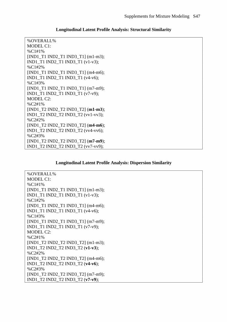
Supplements for Mixture Modeling S47
Longitudinal Latent Profile Analysis: Structural Similarity
%OVERALL%
MODEL C1:
%C1#1%
[IND1_T1 IND2_T1 IND3_T1] (m1-m3);
IND1_T1 IND2_T1 IND3_T1 (v1-v3);
%C1#2%
[IND1_T1 IND2_T1 IND3_T1] (m4-m6);
IND1_T1 IND2_T1 IND3_T1 (v4-v6);
%C1#3%
[IND1_T1 IND2_T1 IND3_T1] (m7-m9);
IND1_T1 IND2_T1 IND3_T1 (v7-v9);
MODEL C2:
%C2#1%
[IND1_T2 IND2_T2 IND3_T2] (m1-m3);
IND1_T2 IND2_T2 IND3_T2 (vv1-vv3);
%C2#2%
[IND1_T2 IND2_T2 IND3_T2] (m4-m6);
IND1_T2 IND2_T2 IND3_T2 (vv4-vv6);
%C2#3%
[IND1_T2 IND2_T2 IND3_T2] (m7-m9);
IND1_T2 IND2_T2 IND3_T2 (vv7-vv9);
Longitudinal Latent Profile Analysis: Dispersion Similarity
%OVERALL%
MODEL C1:
%C1#1%
[IND1_T1 IND2_T1 IND3_T1] (m1-m3);
IND1_T1 IND2_T1 IND3_T1 (v1-v3);
%C1#2%
[IND1_T1 IND2_T1 IND3_T1] (m4-m6);
IND1_T1 IND2_T1 IND3_T1 (v4-v6);
%C1#3%
[IND1_T1 IND2_T1 IND3_T1] (m7-m9);
IND1_T1 IND2_T1 IND3_T1 (v7-v9);
MODEL C2:
%C2#1%
[IND1_T2 IND2_T2 IND3_T2] (m1-m3);
IND1_T2 IND2_T2 IND3_T2 (v1-v3);
%C2#2%
[IND1_T2 IND2_T2 IND3_T2] (m4-m6);
IND1_T2 IND2_T2 IND3_T2 (v4-v6);
%C2#3%
[IND1_T2 IND2_T2 IND3_T2] (m7-m9);
IND1_T2 IND2_T2 IND3_T2 (v7-v9);

Supplements for Mixture Modeling S48
Longitudinal Latent Profile Analysis: Distributional Similarity
In contrast to the multi-group distributional similarity model, which invoked regressions of the
C#k profiles on the CG#k groupings, in longitudinal LPAs, labels are used to constrain the sizes
of the profiles (proportions of cases assigned to each profile) to equality over time points.
%OVERALL%
[C1#1] (p1);
[C1#2] (p2);
[C2#1] (p1);
[C2#2] (p2);
MODEL C1:
%C1#1%
[IND1_T1 IND2_T1 IND3_T1] (m1-m3);
IND1_T1 IND2_T1 IND3_T1 (v1-v3);
%C1#2%
[IND1_T1 IND2_T1 IND3_T1] (m4-m6);
IND1_T1 IND2_T1 IND3_T1 (v4-v6);
%C1#3%
[IND1_T1 IND2_T1 IND3_T1] (m7-m9);
IND1_T1 IND2_T1 IND3_T1 (v7-v9);
MODEL C2:
%C2#1%
[IND1_T2 IND2_T2 IND3_T2] (m1-m3);
IND1_T2 IND2_T2 IND3_T2 (v1-v3);
%C2#2%
[IND1_T2 IND2_T2 IND3_T2] (m4-m6);
IND1_T2 IND2_T2 IND3_T2 (v4-v6);
%C2#3%
[IND1_T2 IND2_T2 IND3_T2] (m7-m9);
IND1_T2 IND2_T2 IND3_T2 (v7-v9);

Supplements for Mixture Modeling S49
Latent Transition Analysis (From a LPA Model of Dispersion Similarity)
In the basic two-occasion LTA, the %OVERALL% section states that membership into the
profiles at the second time point (C2) are conditional on membership in the profiles estimated
at the first time point (C1). This is necessary to estimate the individual transition probabilities
over time. This is the only change (see command in bold) that is required to convert a
longitudinal LPA model with dispersional similarity to a LTA model. However, an important
caveat is that the procedure required to convert a LPA model with distributional similarity to a
LTA is more complex (for details, see Morin & Litalien, 2017:
https://smslabstats.weebly.com/webnotes.html).
%OVERALL%
C2 ON C1;
MODEL C1:
%C1#1%
[IND1_T1 IND2_T1 IND3_T1] (m1-m3);
IND1_T1 IND2_T1 IND3_T1 (v1-v3);
%C1#2%
[IND1_T1 IND2_T1 IND3_T1] (m4-m6);
IND1_T1 IND2_T1 IND3_T1 (v4-v6);
%C1#3%
[IND1_T1 IND2_T1 IND3_T1] (m7-m9);
IND1_T1 IND2_T1 IND3_T1 (v7-v9);
MODEL C2:
%C2#1%
[IND1_T2 IND2_T2 IND3_T2] (m1-m3);
IND1_T2 IND2_T2 IND3_T2 (v1-v3);
%C2#2%
[IND1_T2 IND2_T2 IND3_T2] (m4-m6);
IND1_T2 IND2_T2 IND3_T2 (v4-v6);
%C2#3%
[IND1_T2 IND2_T2 IND3_T2] (m7-m9);
IND1_T2 IND2_T2 IND3_T2 (v7-v9);

Supplements for Mixture Modeling S50
Latent Transition Analysis with Predictors: Relations freely estimated across profiles
and time points
In this model, the effects of the predictors are allowed to differ across time points. Specifically,
separate commands are given for the regression of Time 1 and Time 2 profiles (C1 and C2,
respectively) on the predictors. In addition, the effects of the predictors on the Time 2 profiles
are allowed to differ across the Time 1 profiles in order to assess their specific role in the
prediction of specific profile-to-profile transitions. In other words, this allows for the predictors
to moderate the transition probabilities between C1 and C2 profiles. As in previous models, to
ensure stability, starting values from the previously most similar solution should be used. In
conjunction with this parameterization, users may wish to add TECH15 to the OUTPUT
command to obtain marginal and conditional probabilities (including transition probabilities)
for the latent categorical (i.e., profiles) variables included in the model. As well, conditional
probabilities of individual profile membership and transitions probabilities can be computed for
different values (i.e., mean, ±1SD; see McLarnon et al., 2019) of the predictors to assess
presence of a moderating effect of the predictors using Mplus’ built-in LTA calculator (which
is available from the Mplus drop-down menu of the Mplus Editor window).
%OVERALL%
C2 on C1;
[C1#1] (p1); [C1#2] (p2);
[C2#1] (p1); [C2#2] (p2);
C1 ON Pred1 Pred2;
C2 ON Pred1 Pred2;
MODEL C1:
%C1#1%
[IND1_T1 IND2_T1 IND3_T1] (m1-m3);
IND1_T1 IND2_T1 IND3_T1 (v1-v3);
C2 ON Pred1 Pred2;
%C1#2%
[IND1_T1 IND2_T1 IND3_T1] (m4-m6);
IND1_T1 IND2_T1 IND3_T1 (v4-v6);
C2 ON Pred1 Pred2;
%C1#3%
[IND1_T1 IND2_T1 IND3_T1] (m7-m9);
IND1_T1 IND2_T1 IND3_T1 (v7-v9);
C2 ON Pred1 Pred2;
MODEL C2:
%C2#1%
[IND1_T2 IND2_T2 IND3_T2] (m1-m3);
IND1_T2 IND2_T2 IND3_T2 (v1-v3);
%C2#2%
[IND1_T2 IND2_T2 IND3_T2] (m4-m6);
IND1_T2 IND2_T2 IND3_T2 (v4-v6);
%C2#3%
[IND1_T2 IND2_T2 IND3_T2] (m7-m9);
IND1_T2 IND2_T2 IND3_T2 (v7-v9);
OUTPUT: TECH15;

Supplements for Mixture Modeling S51
Latent Transition Analysis with Predictors: Relations freely estimated across time
points
This model is very similar to the previous one, and has only removed the commands that
specified unique predictor relations across the Time 1 profiles. To ensure stability, start values
from the previously most similar solution should be used.
%OVERALL%
C2 on C1;
[C1#1] (p1);
[C1#2] (p2);
[C2#1] (p1);
[C2#2] (p2);
C1 ON Pred1 Pred2;
C2 ON Pred1 Pred2;
MODEL C1:
%C1#1%
[IND1_T1 IND2_T1 IND3_T1] (m1-m3);
IND1_T1 IND2_T1 IND3_T1 (v1-v3);
%C1#2%
[IND1_T1 IND2_T1 IND3_T1] (m4-m6);
IND1_T1 IND2_T1 IND3_T1 (v4-v6);
%C1#3%
[IND1_T1 IND2_T1 IND3_T1] (m7-m9);
IND1_T1 IND2_T1 IND3_T1 (v7-v9);
MODEL C2:
%C2#1%
[IND1_T2 IND2_T2 IND3_T2] (m1-m3);
IND1_T2 IND2_T2 IND3_T2 (v1-v3);
%C2#2%
[IND1_T2 IND2_T2 IND3_T2] (m4-m6);
IND1_T2 IND2_T2 IND3_T2 (v4-v6);
%C2#3%
[IND1_T2 IND2_T2 IND3_T2] (m7-m9);
IND1_T2 IND2_T2 IND3_T2 (v7-v9);

Supplements for Mixture Modeling S52
Latent Transition Analysis with Predictors: Predictive Similarity
To ensure stability, start values from the previously most similar solution should be used.
%OVERALL%
C2 on C1;
[C1#1] (p1);
[C1#2] (p2);
[C2#1] (p1);
[C2#2] (p2);
C1 ON Pred1 (pr1-pr2);
! one fewer labels than the number of latent profiles is needed
! i.e., the full expansion of the parameters implied here is:
! C1#1 ON Pred1 (pr1); C1#2 ON Pred1 (pr2);
C2 ON Pred1 (pr1-pr2);
C1 ON Pred2 (pr3-pr4);
C2 ON Pred2 (pr3-pr4);
MODEL C1:
%C1#1%
[IND1_T1 IND2_T1 IND3_T1] (m1-m3);
IND1_T1 IND2_T1 IND3_T1 (v1-v3);
%C1#2%
[IND1_T1 IND2_T1 IND3_T1] (m4-m6);
IND1_T1 IND2_T1 IND3_T1 (v4-v6);
%C1#3%
[IND1_T1 IND2_T1 IND3_T1] (m7-m9);
IND1_T1 IND2_T1 IND3_T1 (v7-v9);
MODEL C2:
%C2#1%
[IND1_T2 IND2_T2 IND3_T2] (m1-m3);
IND1_T2 IND2_T2 IND3_T2 (v1-v3);
%C2#2%
[IND1_T2 IND2_T2 IND3_T2] (m4-m6);
IND1_T2 IND2_T2 IND3_T2 (v4-v6);
%C2#3%
[IND1_T2 IND2_T2 IND3_T2] (m7-m9);
IND1_T2 IND2_T2 IND3_T2 (v7-v9);

Supplements for Mixture Modeling S53
Latent Transition Analysis with Outcomes: Relations freely estimated across time points
Here, we use a case where a single outcome, Out, was measured twice, and show how time-
invariant relations could be estimated (i.e., Out1 is the outcome for only the Time 1 profiles,
and Out2 is the same outcome but measured at Time 2). As a separate research question, mean
differences across the different transition patterns could be investigated by applying similarly
structured syntax as described for the multi-group LPA (i.e., develop %C1#1.C2#1% and
provide [Out1]; Out1; commands to allow the outcome to vary across transition patterns. As
well, parameter labels can be applied to each of these outcome means, and then tested for
significant differences using a series of MODEL CONSTRAINTS as illustrated here; see
McLarnon et al., 2019 for an example and syntax). To ensure stability, start values from the
previously most similar solution should be used.
%OVERALL%
C2 on C1;
[C1#1] (p1);
[C1#2] (p2);
[C2#1] (p1);
[C2#2] (p2);
MODEL C1:
%C1#1%
[IND1_T1 IND2_T1 IND3_T1] (m1-m3);
IND1_T1 IND2_T1 IND3_T1 (v1-v3);
[Out1] (oa1); Out1;
%C1#2%
[IND1_T1 IND2_T1 IND3_T1] (m4-m6);
IND1_T1 IND2_T1 IND3_T1 (v4-v6);
[Out1] (oa2); Out1;
%C1#3%
[IND1_T1 IND2_T1 IND3_T1] (m7-m9);
IND1_T1 IND2_T1 IND3_T1 (v7-v9);
[Out1] (oa3); Out1;
MODEL C2:
%C2#1%
[IND1_T2 IND2_T2 IND3_T2] (m1-m3);
IND1_T2 IND2_T2 IND3_T2 (v1-v3);
[Out2] (ob1); Out2;
%C2#2%
[IND1_T2 IND2_T2 IND3_T2] (m4-m6);
IND1_T2 IND2_T2 IND3_T2 (v4-v6);
[Out2] (ob2); Out2;
%C2#3%
[IND1_T2 IND2_T2 IND3_T2] (m7-m9);
IND1_T2 IND2_T2 IND3_T2 (v7-v9);
[Out2] (ob3); Out2;
MODEL CONSTRAINT:
NEW (y12); y12 = oa1-oa2;
NEW (y13); y13 = oa1-oa3;
NEW (y23); y23 = oa2-oa3;
NEW (z12); z12 = ob1-ob2
NEW (z13); z13 = ob1-ob3;
NEW (z23); z23 = ob2-ob3;

Supplements for Mixture Modeling S54
Latent Transition Analysis with Outcomes: Explanatory Similarity
Here, similar labels for the outcomes are applied across Time 1 and Time 2 profiles. As noted
previously, to ensure stability, starting values from the previously most similar solution should
be used.
%OVERALL%
C2 on C1;
[C1#1] (p1);
[C1#2] (p2);
[C2#1] (p1);
[C2#2] (p2);
MODEL C1:
%C1#1%
[IND1_T1 IND2_T1 IND3_T1] (m1-m3);
IND1_T1 IND2_T1 IND3_T1 (v1-v3);
[Out1] (oa1); Out1;
%C1#2%
[IND1_T1 IND2_T1 IND3_T1] (m4-m6);
IND1_T1 IND2_T1 IND3_T1 (v4-v6);
[Out1] (oa2); Out1;
%C1#3%
[IND1_T1 IND2_T1 IND3_T1] (m7-m9);
IND1_T1 IND2_T1 IND3_T1 (v7-v9);
[Out1] (oa3); Out1;
MODEL C2:
%C2#1%
[IND1_T2 IND2_T2 IND3_T2] (m1-m3);
IND1_T2 IND2_T2 IND3_T2 (v1-v3);
[Out2] (oa1); Out2;
%C2#2%
[IND1_T2 IND2_T2 IND3_T2] (m4-m6);
IND1_T2 IND2_T2 IND3_T2 (v4-v6);
[Out2] (oa2); Out2;
%C2#3%
[IND1_T2 IND2_T2 IND3_T2] (m7-m9);
IND1_T2 IND2_T2 IND3_T2 (v7-v9);
[Out2] (oa3); Out2;
MODEL CONSTRAINT:
NEW (y12); y12 = oa1-oa2;
NEW (y13); y13 = oa1-oa3;
NEW (y23); y23 = oa2-oa3;

Supplements for Mixture Modeling S55
Linear Growth Mixture Analysis
In a latent curve model (LCM) estimated in Mplus the “I S |” command serves as a shortcut to
define the latent intercept and slope factors, which is followed by a specification of the time-
varying indicators and their time codes (i.e., λt; their loadings on the intercept and slope factor).
In this input, we request the means of the intercepts and slope factors ([I S];), their variances (I
S;), their covariances (I WITH S;), and all time specific residuals (IND1_T1, IND1_T2,
IND1_T3, IND1_T4, IND1_T5, IND1_T6;) be freely estimated in all profiles. Here, we assume
six repeated measures of a specific indicator (IND1_T1- IND1_T6; which would, of course,
have been defined in the NAMES and USEVARIABLE commands), equally spaced (otherwise
the slope loadings would need to be adjusted to reflect the actual time intervals), with an
intercept located at Time 1. Code to plot these trajectories is provided on the following page.
%OVERALL%
I S | IND1_T1@0 IND1_T2@1 IND1_T3@2 IND1_T4@3 IND1_T5@4 IND1_T6@5;
%C#1%
[I S] (int1 slope1);
I S; I WITH S;
IND1_T1 IND1_T2 IND1_T3 IND1_T4 IND1_T5 IND1_T6;
%C#2%
[I S] (int2 slope2);
I S; I WITH S;
IND1_T1 IND1_T2 IND1_T3 IND1_T4 IND1_T5 IND1_T6;
%C#3%
[I S] (int3 slope3);
I S; I WITH S;
IND1_T1 IND1_T2 IND1_T3 IND1_T4 IND1_T5 IND1_T6;
The following functions provide two alternative ways to plot these trajectories. The first way
uses Mplus’ default plotting procedure. The second function requires some additional user
customization, but advantageously, can provide a plot with confidence intervals around the
trajectories in each profile group, and is specified within a MODEL CONSTRAINT procedure.
With the PLOT command, arbitrary labels are used to define the trajectories to be plotted.
Conceivably there should be one for each profile group, and there are three in this example. The
LOOP function then defines an arbitrary label for a variable that will be used in computing the
equations for each trajectory. Here, “Time” is used to reflect the notion of growth curves. The
rest of the LOOP function requests that “Time” is given an interval of 0 to 5, and is increased
by 0.1 increments. So, in the computation of the following Profile1 trajectory, values for “Time”
between 0 and 5, increasing at 0.1 increments will be included in the equation, and then the
resulting values will be plotted. Here, the interval of 0 to 5 was chosen to reflect plotted the
trajectories to start at same point as the measurement occasions (i.e., the intercept, before any
linear change occurred), and six measures were obtained. These values can be adjusted for any
particular application. Critically, this approach also requires the labeling of the mean intercept
and slope mean parameters in each class (i.e., int1 and slope1) to be used in the calculations of
the trajectories.
PLOT:
TYPE IS PLOT3;
SERIES = IND1_T1 IND1_T2 IND1_T3 IND1_T4 IND1_T5 IND1_T6 (*);
MODEL CONSTRAINT:
PLOT(Profile1 Profile2 Profile3);
LOOP(Time,0,5,0.1);
Profile1 = int1+Time*slope1;
Profile2 = int2+Time*slope2;
Profile3 = int3+Time*slope3;

Supplements for Mixture Modeling S56
As noted in our main description of linear growth mixture models, simpler parameterizations
are possible should the above, fully variant model fail to converge on proper solutions. Our
preference is to test these alternative models in the following order: 1. Alternative A – Homoscedastic Residuals (equal across time points) 2. Alternative B – Class-Invariant Residuals 3. Alternative C – Class-Invariant Latent Variance-Covariance Matrix 4. Alternative D – Class-Invariant Homoscedastic Residuals (equal across time
points) 5. Alternative E – Class-Invariant Latent Variance-Covariance Matrix and
Homoscedastic Residuals 6. Alternative – Class-Invariant Latent Variance-Covariance Matrix and Class-
Invariant Residuals 7. Alternative G – Class-Invariant Latent Variance-Covariance Matrix and Class-
Invariant Homoscedastic Residuals
Alternative A – Homoscedastic Residuals (equal across time points)
%OVERALL%
I S | IND1_T1@0 IND1_T2@1 IND1_T3@2 IND1_T4@3 IND1_T5@4 IND1_T6@5;
%C#1%
[I S];
I S; I WITH S;
IND1_T1 IND1_T2 IND1_T3 IND1_T4 IND1_T5 IND1_T6 (R1);
%C#2%
[I S];
I S; I WITH S;
IND1_T1 IND1_T2 IND1_T3 IND1_T4 IND1_T5 IND1_T6 (R2);
%C#3%
[I S];
I S; I WITH S;
IND1_T1 IND1_T2 IND1_T3 IND1_T4 IND1_T5 IND1_T6 (R3);

Supplements for Mixture Modeling S57
Alternative B – Class-Invariant Residuals
%OVERALL%
I S | IND1_T1@0 IND1_T2@1 IND1_T3@2 IND1_T4@3 IND1_T5@4 IND1_T6@5;
%C#1%
[I S];
I S; I WITH S;
%C#2%
[I S];
I S; I WITH S;
%C#3%
[I S];
I S; I WITH S;
Alternative C – Class-Invariant Latent Variance-Covariance Matrix
%OVERALL%
I S | IND1_T1@0 IND1_T2@1 IND1_T3@2 IND1_T4@3 IND1_T5@4 IND1_T6@5;
%C#1%
[I S];
IND1_T1 IND1_T2 IND1_T3 IND1_T4 IND1_T5 IND1_T6;
%C#2%
[I S];
IND1_T1 IND1_T2 IND1_T3 IND1_T4 IND1_T5 IND1_T6;
%C#3%
[I S];
IND1_T1 IND1_T2 IND1_T3 IND1_T4 IND1_T5 IND1_T6;

Supplements for Mixture Modeling S58
Alternative D – Class-Invariant Homoscedastic Residuals (equal across time points)
%OVERALL%
I S | IND1_T1@0 IND1_T2@1 IND1_T3@2 IND1_T4@3 IND1_T5@4 IND1_T6@5;
%C#1%
[I S];
I S; I WITH S;
IND1_T1 IND1_T2 IND1_T3 IND1_T4 IND1_T5 IND1_T6 (R1);
%C#2%
[I S];
I S; I WITH S;
IND1_T1 IND1_T2 IND1_T3 IND1_T4 IND1_T5 IND1_T6 (R1);
%C#3%
[I S];
I S; I WITH S;
IND1_T1 IND1_T2 IND1_T3 IND1_T4 IND1_T5 IND1_T6 (R1);
Alternative E – Class-Invariant Latent Variance-Covariance Matrix and Homoscedastic
Residuals
%OVERALL%
I S | IND1_T1@0 IND1_T2@1 IND1_T3@2 IND1_T4@3 IND1_T5@4 IND1_T6@5;
%C#1%
[I S];
IND1_T1 IND1_T2 IND1_T3 IND1_T4 IND1_T5 IND1_T6 (R1);
%C#2%
[I S];
IND1_T1 IND1_T2 IND1_T3 IND1_T4 IND1_T5 IND1_T6 (R2);
%C#3%
[I S];
IND1_T1 IND1_T2 IND1_T3 IND1_T4 IND1_T5 IND1_T6 (R3);

Supplements for Mixture Modeling S59
Alternative F – Class-Invariant Latent Variance-Covariance Matrix and Class-Invariant
Residuals
Note that this is the default specification within Mplus.
%OVERALL%
I S | IND1_T1@0 IND1_T2@1 IND1_T3@2 IND1_T4@3 IND1_T5@4 IND1_T6@5;
%C#1%
[I S];
%C#2%
[I S];
%C#3%
[I S];
Alternative G – Class-Invariant Latent Variance-Covariance Matrix and Class-Invariant
Homoscedastic Residuals
%OVERALL%
I S | IND1_T1@0 IND1_T2@1 IND1_T3@2 IND1_T4@3 IND1_T5@4 IND1_T6@5;
%C#1%
[I S];
IND1_T1 IND1_T2 IND1_T3 IND1_T4 IND1_T5 IND1_T6 (R1);
%C#2%
[I S];
IND1_T1 IND1_T2 IND1_T3 IND1_T4 IND1_T5 IND1_T6 (R1);
%C#3%
[I S];
IND1_T1 IND1_T2 IND1_T3 IND1_T4 IND1_T5 IND1_T6 (R1);

Supplements for Mixture Modeling S60
Quadratic Growth Mixture Analysis
A quadratic slope factor (Q) can be added to allow for curvilinear trends. The following code
provides the commands for the fully variant model, but the sequential testing described above
can be applied to derive simpler parameterizations should issues of convergence or statistical
adequacy result. The same two plotting procedures, noted above, can be applied, but we detail
the LOOP approach below given the need for more user customization. If further polynomial
functions are required, their factor label (i.e., CU for cubic [labeling it C would duplicate the
label assigned to the latent profiles and would not be allowed], etc.) would just be added to the
growth statement before the | symbol, similar to the difference between the linear and quadratic
functions. Additional commands for the extra polynomial functions would then be added to
each profile-specific section.
%OVERALL%
I S Q | IND1_T1@0 IND1_T2@1 IND1_T3@2 IND1_T4@3 IND1_T5@4 IND1_T6@5;
%C#1%
I S Q;
[I S Q] (int1 linear1 quad1);
I WITH S Q;
S WITH Q;
IND1_T1 IND1_T2 IND1_T3 IND1_T4 IND1_T5 IND1_T6;
%C#2%
I S Q;
[I S Q] (int2 linear2 quad2);
I WITH S Q;
S WITH Q;
IND1_T1 IND1_T2 IND1_T3 IND1_T4 IND1_T5 IND1_T6;
%C#3%
I S Q;
[I S Q] (int3 linear3 quad3);
I WITH S Q;
S WITH Q;
IND1_T1 IND1_T2 IND1_T3 IND1_T4 IND1_T5 IND1_T6;
MODEL CONSTRAINT:
PLOT(Profile1 Profile2 Profile3);
LOOP(Time,0,5,0.1);
Profile1 = int1+Time*linear1+quad1*Time**2;
Profile2 = int2+Time*linear2+quad2*Time**2;
Profile3 = int3+Time*linear3+quad3*Time**2;

Supplements for Mixture Modeling S61
Piecewise Growth Mixture Analysis
A piecewise growth model implements multiple slope factors to account for distinct ‘before
and after’ trajectories that may be exhibited. Two linear slope factors (here, S1 and S2) can be
defined to represent linear changes before and after a transition point. In this example, the
second slope or trajectory begins at Time 4. As in previous models, simpler parameterizations
are possible to implement should they be required. As well, piecewise models can be specified
to include curvilinear trajectories before and/or after the transition point. For plotting, the LOOP
function would not be readily available because Mplus can only allow for a single LOOP
command in an analysis (it may however be possible to adjust the starting and ending points of
the LOOP and import the calculated plot data from separate LOOPs into Microsoft Excel and
replot the trajectories there, but this is not an overly straightforward procedure). However, the
built-in PLOT command can be used straightforwardly to visualize the functions.
%OVERALL%
I S1 | IND1_T1@0 IND1_T2@1 IND1_T3@2 IND1_T4@2 IND1_T5@2 IND1_T6@2;
I S2 | IND1_T1@0 IND1_T2@0 IND1_T3@0 IND1_T4@1 IND1_T5@2 IND1_T6@3;
%C#1%
I S1 S2;
[I S1 S2];
I WITH S1 S2;
S1 WITH S2;
IND1_T1 IND1_T2 IND1_T3 IND1_T4 IND1_T5 IND1_T6;
%C#2%
I S1 S2;
[I S1 S2];
I WITH S1 S2;
S1 WITH S2;
IND1_T1 IND1_T2 IND1_T3 IND1_T4 IND1_T5 IND1_T6;
%C#3%
I S1 S2;
[I S1 S2];
I WITH S1 S2;
S1 WITH S2;
IND1_T1 IND1_T2 IND1_T3 IND1_T4 IND1_T5 IND1_T6;
PLOT:
TYPE IS PLOT3;
SERIES = IND1_T1 IND1_T2 IND1_T3 IND1_T4 IND1_T5 IND1_T6 (*);

Supplements for Mixture Modeling S62
Latent Basis Growth Mixture Analysis
In a latent basis model, two loadings (typically the first and last) need to be fixed, respectively,
to 0 and 1 (i.e., using @0 and @1) while the other loadings are freely estimated (i.e., using *).
Here, we request that the loadings for the Time 2, 3, 4, and 5 assessments be freely estimated
in all profiles by repeating these commands in the profile-specific sections. As in previous
models, simpler parameterizations are possible to implement should they be required. The
LOOP function will not adequately demonstrate the growth trajectories because the differing
factor loadings on the slope factor (reflecting non-linearity) cannot be taken into account (i.e.,
the slope factor in a latent basis model only reflects the total change occurring over time). The
PLOT command can therefore be used to visualize the growth trajectories.
%OVERALL%
I S | IND1_T1@0 IND1_T2* IND1_T3* IND1_T4* IND1_T5* IND1_T6@1;
%C#1%
I S | IND1_T1@0 IND1_T2* IND1_T3* IND1_T4* IND1_T5* IND1_T6@1;
I S;
[I S] (int1 slope1);
I WITH S;
IND1_T1 IND1_T2 IND1_T3 IND1_T4 IND1_T5 IND1_T6;
%C#2%
I S | IND1_T1@0 IND1_T2* IND1_T3* IND1_T4* IND1_T5* IND1_T6@1;
I S;
[I S] (int2 slope2);
I WITH S;
IND1_T1 IND1_T2 IND1_T3 IND1_T4 IND1_T5 IND1_T6;
%C#3%
I S | IND1_T1@0 IND1_T2* IND1_T3* IND1_T4* IND1_T5* IND1_T6@1;
I S;
[I S] (int3 slope3);
I WITH S;
IND1_T1 IND1_T2 IND1_T3 IND1_T4 IND1_T5 IND1_T6;
TYPE IS PLOT3:
SERIES = IND1_T1 IND1_T2 IND1_T3 IND1_T4 IND1_T5 IND1_T6 (*);

Supplements for Mixture Modeling S63
Mehta and West (2000) Test
As change may occur differentially for cases that differ on tenure or age (at the first assessment),
bias may be introduced into the meaning and interpretation of the latent slope. Mehta and West
(2000) advised assessing the relation that age (or any other meaningful time-related variable)
has on the estimate of the latent slope. In particular, they noted that variations in individuals’
initial age/tenure/grade can be considered negligible when the following two conditions are
met: (1) the regression of the intercept of a LCM on age is equal to the mean of the slope factor,
and (2) the regression of the slope factor on age is equal to zero. Testing these conditions
involves contrasting a typical, unrestricted LCM model that incorporates age as a predictor of
the intercept and slope factors to a model in which these two conditions are imposed. If the
more constrained model fits the data as well as the first model (as assessed via typical goodness-
of-fit indices), then the impact of age can be considered to be negligible.
Initial Model:
VARIABLE:
NAMES = ID Age IND1_T1 IND1_T2 IND1_T3 IND1_T4 IND1_T5 IND1_T6;
USEVARIABLES = Age IND1_T1 IND1_T2 IND1_T3 IND1_T4 IND1_T5 IND1_T6;
MISSING = all (999);
IDVARIABLE = ID;
ANALYSIS:
ESTIMATOR = MLR;
MODEL:
I S | IND1_T1@0 IND1_T2@1 IND1_T3@2 IND1_T4@3 IND1_T5@4 IND1_T6@5;
IND1_T1 IND1_T2 IND1_T3 IND1_T4 IND1_T5 IND1_T6;
I ON Age;
S ON Age;
Constrained Model:
MODEL:
I S | IND1_T1@0 IND1_T2@1 IND1_T3@2 IND1_T4@3 IND1_T5@4 IND1_T6@5;
IND1_T1 IND1_T2 IND1_T3 IND1_T4 IND1_T5 IND1_T6;
I ON Age (c1);
[S] (c1);
S ON Age@0;

Supplements for Mixture Modeling S64
Age-Defined Linear Growth Mixture Analysis
To estimate a growth mixture analysis where age (or any other variable differing across
individuals) is used to define the time codes (i.e., factor loadings for the latent slope), this
variable needs to be identified using the CONSTRAINT command of the VARIABLE section
of the syntax. The CONSTRAINT command identifies variables used only in the MODEL
CONSTRAINT section of the syntax. In the age-defined growth model, the loadings on the
slope factor (representing the time code), rather than being fixed to specific values, are freely
estimated and assigned a label (here, L1 to L6). Using this approach involves relying on the
complete specification of the LCM model (without being able to use the shortcut function
associated with the | symbol). To apply a complete specification, one also has to constrain the
time specific intercepts to 0, and request the free estimation of the intercept and slope factor
means in the %OVERALL% section. In this example, we define trajectories on the basis of
individually-varying ages (coded in years), and want to set the intercept of the trajectories to
that of a 25-year old (hence the subtraction of 25 in each of the MODEL CONSTRAINT
equations; this corresponds to the age of the youngest employee at Time 1). Measurement
occurred at annual intervals that were equal for all participants. If measurement intervals also
differed across participants, then one AGE variable would be required for each time of
measurement (i.e., Age_T1, Age_T2, etc.). With this approach, time-specific residuals should
be specified as homoscedastic (equal across time points) as the alternative approach of allowing
them to differ across time of measurement would be inconsistent with the definition of time
codes that ignore the time of measurement. The default PLOT function does not work in this
context, so that the trajectories would need to be plotted with the LOOP function described
earlier, or graphed manually. This model is illustrated on the following page:
VARIABLE:
NAMES = ID Age IND1_T1 IND1_T2 IND1_T3 IND1_T4 IND1_T5 IND1_T6;
USEVARIABLES = IND1_T1 IND1_T2 IND1_T3 IND1_T4 IND1_T5 IND1_T6;
MISSING = all (999);
IDVARIABLE = ID;
CONSTRAINT = Age;
CLASSES = C(3);
ANALYSIS:
TYPE = MIXTURE COMPLEX; ESTIMATOR = MLR;
PROCESS = 3; STARTS = 3000 100; STITERATIONS = 100;
MODEL:
%OVERALL%
I BY IND1_T1@1 IND1_T2@1 IND1_T3@1 IND1_T4@1 IND1_T5@1 IND1_T6@1;
S BY IND1_T1* (L1)
IND1_T2 (L2)
IND1_T3 (L3)
IND1_T4 (L4)
IND1_T5 (L5)
IND1_T6 (L6);
I S; I WITH S; [I S];
[IND1_T1@0 IND1_T2@0 IND1_T3@0 IND1_T4@0 IND1_T5@0 IND1_T6@0];
IND1_T1 IND1_T2 IND1_T3 IND1_T4 IND1_T5 IND1_T6;

Supplements for Mixture Modeling S65
%C#1%
I S; I WITH S;
[I S] (int1 slope1);
IND1_T1 IND1_T2 IND1_T3 IND1_T4 IND1_T5 IND1_T6 (r1);
%C#2%
I S; I WITH S;
[I S] (int2 slope2);
IND1_T1 IND1_T2 IND1_T3 IND1_T4 IND1_T5 IND1_T6 (r2);
%C#3%
I S; I WITH S;
[I S] (int3 slope3);
IND1_T1 IND1_T2 IND1_T3 IND1_T4 IND1_T5 IND1_T6 (r3);
MODEL CONSTRAINT:
L1 = AGE - 25;
L2 = AGE - 25 + 1;
L3 = AGE - 25 + 2;
L4 = AGE - 25 + 3;
L5 = AGE - 25 + 4;
L6 = AGE - 25 + 5;
MODEL CONSTRAINT:
PLOT(Profile1 Profile2 Profile3); LOOP(Time,0,5,0.1);
Profile1 = int1+Time*slope1;
Profile2 = int2+Time*slope2;
Profile3 = int3+Time*slope3;

Supplements for Mixture Modeling S66
Age-Defined Quadratic Growth Mixture Analysis
A similar approach can be used for a quadratic model (or any other polynomial models, where
the form of the polynomial would apply to the equations used within the MODEL
CONSTRAINT; i.e., the functions are squared in the below quadratic formulation). As above,
the LOOP function or manual plotting of the resulting trajectories would be needed.
MODEL:
%OVERALL%
I BY IND1_T1@1 IND1_T2@1 IND1_T3@1 IND1_T4@1 IND1_T5@1 IND1_T6@1;
S BY IND1_T1* (L1)
IND1_T2 (L2)
IND1_T3 (L3)
IND1_T4 (L4)
IND1_T5 (L5)
IND1_T6 (L6);
Q BY IND1_T1* (Q1)
IND1_T2 (Q2)
IND1_T3 (Q3)
IND1_T4 (Q4)
IND1_T5 (Q5)
IND1_T6 (Q6);
I S Q; I WITH S Q; S WITH Q;
[I S Q];
[IND1_T1@0 IND1_T2@0 IND1_T3@0 IND1_T4@0 IND1_T5@0 IND1_T6@0];
IND1_T1 IND1_T2 IND1_T3 IND1_T4 IND1_T5 IND1_T6;
%C#1%
I S Q; I WITH S Q; S WITH Q;
[I S Q] (int1 linear1 quad1);
IND1_T1 IND1_T2 IND1_T3 IND1_T4 IND1_T5 IND1_T6 (r1);
%C#2%
I S Q; I WITH S Q; S WITH Q;
[I S Q] (int2 linear2 quad2);
IND1_T1 IND1_T2 IND1_T3 IND1_T4 IND1_T5 IND1_T6 (r2);
%C#3%
I S Q; I WITH S Q; S WITH Q;
[I S Q] (int3 linear3 quad3);
IND1_T1 IND1_T2 IND1_T3 IND1_T4 IND1_T5 IND1_T6 (r3);
MODEL CONSTRAINT:
L1 = AGE - 25;
L2 = AGE - 25 + 1;
L3 = AGE - 25 + 2;
L4 = AGE - 25 + 3;
L5 = AGE - 25 + 4;
L6 = AGE - 25 + 5;
Q1 = (AGE - 25)**2;
Q2 = (AGE - 25+1)**2;
Q3 = (AGE - 25+2)**2;
Q4 = (AGE - 25+3)**2;
Q5 = (AGE - 25+4)**2;
Q6 = (AGE - 25+5)**2;
MODEL CONSTRAINT:
PLOT(Profile1 Profile2 Profile3);
LOOP(Time,0,5,0.1);
Profile1 = int1+Time*linear1+quad1*Time**2;
Profile2 = int2+Time*linear2+quad2*Time**2;
Profile3 = int3+Time*linear3+quad3*Time**2;

Supplements for Mixture Modeling S67
Growth Mixture Analysis: Time-Invariant Predictors
The following models involve contrasting a model in which the relations for the time-invariant
predictors are restricted to zero (i.e., the null effects model), and alternative models in which
(a) the predictors may only potentially influence class membership, (b) the predictors can
influence class membership, and also the intercept and slope factors, but that the intercept and
slope relations are held equal across profile groups, and (c) the predictors can influence class
membership, and can also influence the intercept and slope freely across profiles. Adjustments
to the syntax to facilitate these different models are highlighted in bold below.
Null-Effects Model
%OVERALL%
I S | IND1_T1@0 IND1_T2@1 IND1_T3@2 IND1_T4@3 IND1_T5@4 IND1_T6@5;
C ON Pred1@0 Pred2@0;
I ON Pred1@0 Pred2@0;
S ON Pred1@0 Pred2@0;
%C#1%
[I S];
I S; I WITH S;
IND1_T1 IND1_T2 IND1_T3 IND1_T4 IND1_T5 IND1_T6;
%C#2%
[I S];
I S; I WITH S;
IND1_T1 IND1_T2 IND1_T3 IND1_T4 IND1_T5 IND1_T6;
%C#3%
[I S];
I S; I WITH S;
IND1_T1 IND1_T2 IND1_T3 IND1_T4 IND1_T5 IND1_T6;
Alternative A – Freely Estimated Effects on Class Membership Only
%OVERALL%
I S | IND1_T1@0 IND1_T2@1 IND1_T3@2 IND1_T4@3 IND1_T5@4 IND1_T6@5;
C ON Pred1 Pred2;
I ON Pred1@0 Pred2@0;
S ON Pred1@0 Pred2@0;
%C#1%
[I S];
I S; I WITH S;
IND1_T1 IND1_T2 IND1_T3 IND1_T4 IND1_T5 IND1_T6;
%C#2%
[I S];
I S; I WITH S;
IND1_T1 IND1_T2 IND1_T3 IND1_T4 IND1_T5 IND1_T6;
%C#3%
[I S];
I S; I WITH S;
IND1_T1 IND1_T2 IND1_T3 IND1_T4 IND1_T5 IND1_T6;

Supplements for Mixture Modeling S68
Alternative B – Effects on Class Membership and Class-Invariant Effects on the Growth
Factors
%OVERALL%
I S | IND1_T1@0 IND1_T2@1 IND1_T3@2 IND1_T4@3 IND1_T5@4 IND1_T6@5;
C ON Pred1 Pred2;
I ON Pred1 Pred2;
S ON Pred1 Pred2;
%C#1%
[I S];
I S; I WITH S;
IND1_T1 IND1_T2 IND1_T3 IND1_T4 IND1_T5 IND1_T6;
%C#2%
[I S];
I S; I WITH S;
IND1_T1 IND1_T2 IND1_T3 IND1_T4 IND1_T5 IND1_T6;
%C#3%
[I S];
I S; I WITH S;
IND1_T1 IND1_T2 IND1_T3 IND1_T4 IND1_T5 IND1_T6;
Alternative C – Effects on Class Membership and Class-Varying Effects on the Growth
Factors
%OVERALL%
I S | IND1_T1@0 IND1_T2@1 IND1_T3@2 IND1_T4@3 IND1_T5@4 IND1_T6@5;
C ON Pred1 Pred2;
I ON Pred1 Pred2;
S ON Pred1 Pred2;
%C#1%
[I S];
I S; I WITH S;
IND1_T1 IND1_T2 IND1_T3 IND1_T4 IND1_T5 IND1_T6;
I ON Pred1 Pred2;
S ON Pred1 Pred2;
%C#2%
[I S];
I S; I WITH S;
IND1_T1 IND1_T2 IND1_T3 IND1_T4 IND1_T5 IND1_T6;
I ON Pred1 Pred2;
S ON Pred1 Pred2;
%C#3%
[I S];
I S; I WITH S;
IND1_T1 IND1_T2 IND1_T3 IND1_T4 IND1_T5 IND1_T6;
I ON Pred1 Pred2;
S ON Pred1 Pred2;

Supplements for Mixture Modeling S69
Growth Mixture Analysis: Time-Invariant Outcomes
These analyses follow from the LPA with outcomes models described earlier.
%OVERALL%
I S | IND1_T1@0 IND1_T2@1 IND1_T3@2 IND1_T4@3 IND1_T5@4 IND1_T6@5;
%C#1%
[I S];
I S; I WITH S;
IND1_T1 IND1_T2 IND1_T3 IND1_T4 IND1_T5 IND1_T6;
[Out1] (oa1);
[Out2] (ob1);
Out1;
Out2;
%C#2%
[I S];
I S; I WITH S;
IND1_T1 IND1_T2 IND1_T3 IND1_T4 IND1_T5 IND1_T6;
[Out1] (oa2);
[Out2] (ob2);
Out1;
Out2;
%C#3%
[I S];
I S; I WITH S;
IND1_T1 IND1_T2 IND1_T3 IND1_T4 IND1_T5 IND1_T6;
[Out1] (oa3);
[Out2] (ob3);
Out1;
Out2;
MODEL CONSTRAINT:
NEW (y12);
y12 = oa1-oa2;
NEW (y13);
y13 = oa1-oa3;
NEW (y23);
y23 = oa2-oa3;
NEW (z12);
z12 = ob1-ob2
NEW (z13);
z13 = ob1-ob3;
NEW (z23);
z23 = ob2-ob3;

Supplements for Mixture Modeling S70
Growth Mixture Analysis: Time-Varying Predictors
The following series of models presents a potential framework that can be used for time-varying
predictors. In contrast to the previous predictor models, where the predictors targeted profile
membership, the intercept and slope factors, or both, time-varying predictors target the focal
indicators that have been measured at each occasion, respectively. As above, these can also
involve a contrast between a model in which the relations for the time-varying predictors are
restricted to zero (i.e., the null effects model), and alternative models that include (a) effects
that are free to vary across time points, but equal across profiles, (b) effects that are free to vary
across time points and profiles, (c) effects that are free to vary across profiles but not time
points, and (d) effects constrained to equality across time points and profiles.
Null-Effects Model
%OVERALL%
I S | IND1_T1@0 IND1_T2@1 IND1_T3@2 IND1_T4@3 IND1_T5@4 IND1_T6@5;
IND1_T1 ON PredT1@0;
IND1_T2 ON PredT2@0;
IND1_T3 ON PredT3@0;
IND1_T4 ON PredT4@0;
IND1_T5 ON PredT5@0;
IND1_T6 ON PredT6@0;
[PredT1] (m1); [PredT2] (m2); [PredT3] (m3); [PredT4] (m4); [PredT5] (m5); [PredT6] (m6);
%C#1%
[I S];
I S; I WITH S;
IND1_T1 IND1_T2 IND1_T3 IND1_T4 IND1_T5 IND1_T6;
%C#2%
[I S];
I S; I WITH S;
IND1_T1 IND1_T2 IND1_T3 IND1_T4 IND1_T5 IND1_T6;
%C#3%
[I S];
I S; I WITH S;
IND1_T1 IND1_T2 IND1_T3 IND1_T4 IND1_T5 IND1_T6;

Supplements for Mixture Modeling S71
Alternative A – Effects Free to Vary Across Time Points but Equal Across Profiles
%OVERALL%
I S | IND1_T1@0 IND1_T2@1 IND1_T3@2 IND1_T4@3 IND1_T5@4 IND1_T6@5;
IND1_T1 ON PredT1;
IND1_T2 ON PredT2;
IND1_T3 ON PredT3;
IND1_T4 ON PredT4;
IND1_T5 ON PredT5;
IND1_T6 ON PredT6;
[PredT1] (m1); [PredT2] (m2); [PredT3] (m3); [PredT4] (m4); [PredT5] (m5); [PredT6] (m6);
%C#1%
[I S];
I S; I WITH S;
IND1_T1 IND1_T2 IND1_T3 IND1_T4 IND1_T5 IND1_T6;
%C#2%
[I S];
I S; I WITH S;
IND1_T1 IND1_T2 IND1_T3 IND1_T4 IND1_T5 IND1_T6;
%C#3%
[I S];
I S; I WITH S;
IND1_T1 IND1_T2 IND1_T3 IND1_T4 IND1_T5 IND1_T6;

Supplements for Mixture Modeling S72
Alternative B – Effects Free to Vary Across Time Points and Profiles
%OVERALL%
I S | IND1_T1@0 IND1_T2@1 IND1_T3@2 IND1_T4@3 IND1_T5@4 IND1_T6@5;
IND1_T1 ON PredT1;
IND1_T2 ON PredT2;
IND1_T3 ON PredT3;
IND1_T4 ON PredT4;
IND1_T5 ON PredT5;
IND1_T6 ON PredT6;
[PredT1] (m1); [PredT2] (m2); [PredT3] (m3); [PredT4] (m4); [PredT5] (m5); [PredT6] (m6);
%C#1%
[I S];
I S; I WITH S;
IND1_T1 IND1_T2 IND1_T3 IND1_T4 IND1_T5 IND1_T6;
IND1_T1 ON PredT1;
IND1_T2 ON PredT2;
IND1_T3 ON PredT3;
IND1_T4 ON PredT4;
IND1_T5 ON PredT5;
IND1_T6 ON PredT6;
%C#2%
[I S];
I S; I WITH S;
IND1_T1 IND1_T2 IND1_T3 IND1_T4 IND1_T5 IND1_T6;
IND1_T1 ON PredT1;
IND1_T2 ON PredT2;
IND1_T3 ON PredT3;
IND1_T4 ON PredT4;
IND1_T5 ON PredT5;
IND1_T6 ON PredT6;
%C#3%
[I S];
I S; I WITH S;
IND1_T1 IND1_T2 IND1_T3 IND1_T4 IND1_T5 IND1_T6;
IND1_T1 ON PredT1;
IND1_T2 ON PredT2;
IND1_T3 ON PredT3;
IND1_T4 ON PredT4;
IND1_T5 ON PredT5;
IND1_T6 ON PredT6;

Supplements for Mixture Modeling S73
Alternative C – Effects Free to Vary Across Profiles but Not Time Points
%OVERALL%
I S | IND1_T1@0 IND1_T2@1 IND1_T3@2 IND1_T4@3 IND1_T5@4 IND1_T6@5;
IND1_T1 ON PredT1;
IND1_T2 ON PredT2;
IND1_T3 ON PredT3;
IND1_T4 ON PredT4;
IND1_T5 ON PredT5;
IND1_T6 ON PredT6;
[PredT1] (m1); [PredT2] (m2); [PredT3] (m3); [PredT4] (m4); [PredT5] (m5); [PredT6] (m6);
%C#1%
[I S];
I S; I WITH S;
IND1_T1 IND1_T2 IND1_T3 IND1_T4 IND1_T5 IND1_T6;
IND1_T1 ON PredT1 (r1);
IND1_T2 ON PredT2 (r1);
IND1_T3 ON PredT3 (r1);
IND1_T4 ON PredT4 (r1);
IND1_T5 ON PredT5 (r1);
IND1_T6 ON PredT6 (r1);
%C#2%
[I S];
I S; I WITH S;
IND1_T1 IND1_T2 IND1_T3 IND1_T4 IND1_T5 IND1_T6;
IND1_T1 ON PredT1 (r2);
IND1_T2 ON PredT2 (r2);
IND1_T3 ON PredT3 (r2);
IND1_T4 ON PredT4 (r2);
IND1_T5 ON PredT5 (r2);
IND1_T6 ON PredT6 (r2);
%C#3%
[I S];
I S; I WITH S;
IND1_T1 IND1_T2 IND1_T3 IND1_T4 IND1_T5 IND1_T6;
IND1_T1 ON PredT1 (r3);
IND1_T2 ON PredT2 (r3);
IND1_T3 ON PredT3 (r3);
IND1_T4 ON PredT4 (r3);
IND1_T5 ON PredT5 (r3);
IND1_T6 ON PredT6 (r3);

Supplements for Mixture Modeling S74
Alternative D – Effects Constrained to Equality Across Time Points and Profiles
%OVERALL%
I S | IND1_T1@0 IND1_T2@1 IND1_T3@2 IND1_T4@3 IND1_T5@4 IND1_T6@5;
IND1_T1 ON PredT1 (r1);
IND1_T2 ON PredT2 (r1);
IND1_T3 ON PredT3 (r1);
IND1_T4 ON PredT4 (r1);
IND1_T5 ON PredT5 (r1);
IND1_T6 ON PredT6 (r1);
[PredT1] (m1); [PredT2] (m2); [PredT3] (m3); [PredT4] (m4); [PredT5] (m5); [PredT6] (m6);
%C#1%
[I S];
I S; I WITH S;
IND1_T1 IND1_T2 IND1_T3 IND1_T4 IND1_T5 IND1_T6;
%C#2%
[I S];
I S; I WITH S;
IND1_T1 IND1_T2 IND1_T3 IND1_T4 IND1_T5 IND1_T6;
%C#3%
[I S];
I S; I WITH S;
IND1_T1 IND1_T2 IND1_T3 IND1_T4 IND1_T5 IND1_T6;

Supplements for Mixture Modeling S75
Growth Mixture Analysis: Time-Varying Outcomes
The final series of models we present can be leveraged to investigate time-varying outcome
relations. These are similar to the previous set of models that specified time-varying predictors.
In contrast to the models where time-invariant outcomes were specified, these outcome
relations are specified as a function of the focal indicators that have been measured at each
occasion. Further, in this case the main interest might be to examine the regression relations
between the time-specific indicators and the time-specific outcomes, rather than mean
differences in the outcomes across the mixture groups (though they are still estimated, and may
of course be of substantive interest). As in the time-varying predictor models, determining an
appropriate, optimal model can involve contrasts between a model in which the relations for
the time-varying predictors are restricted to zero (i.e., the null effects model), and alternative
models that include (a) effects that are free to vary across time points, but equal across profiles,
(b) effects that are free to vary across time points and profiles, (c) effects that are free to vary
across profiles but not time points, and (d) effects constrained to equality across time points and
profiles. In the following examples, we (a) freely estimate the full regression equation (which
includes the slope, intercepts, and residuals) associated with the time-varying outcomes and
allow them to differ, and (b) constrain these three components (slope, intercepts, and residuals)
to equality across profiles and time points. Simpler models only specifying differences in
regression slopes can also be estimated, in which case the syntax presented in greyscale should
be omitted. Alternatively, equality constraints can be imposed and tested in sequence (on the
slopes, then intercepts, then residuals) once the optimal model has been selected.
Null-Effects Model
%OVERALL%
I S | IND1_T1@0 IND1_T2@1 IND1_T3@2 IND1_T4@3 IND1_T5@4 IND1_T6@5;
OutT1 ON IND1_T1@0;
OutT2 ON IND1_T2@0;
OutT3 ON IND1_T3@0;
OutT4 ON IND1_T4@0;
OutT5 ON IND1_T5@0;
OutT6 ON IND1_T6@0;
[OutT1] (m1); [OutT2] (m2); [OutT3] (m3); [OutT4] (m4); [OutT5] (m5); [OutT6] (m6);
%C#1%
[I S];
I S; I WITH S;
IND1_T1 IND1_T2 IND1_T3 IND1_T4 IND1_T5 IND1_T6;
%C#2%
[I S];
I S; I WITH S;
IND1_T1 IND1_T2 IND1_T3 IND1_T4 IND1_T5 IND1_T6;
%C#3%
[I S];
I S; I WITH S;
IND1_T1 IND1_T2 IND1_T3 IND1_T4 IND1_T5 IND1_T6;

Supplements for Mixture Modeling S76
Alternative A – Effects Free to Vary Across Time Points but Equal Across Profiles
%OVERALL%
I S | IND1_T1@0 IND1_T2@1 IND1_T3@2 IND1_T4@3 IND1_T5@4 IND1_T6@5;
OutT1 ON IND1_T1;
OutT2 ON IND1_T2;
OutT3 ON IND1_T3;
OutT4 ON IND1_T4;
OutT5 ON IND1_T5;
OutT6 ON IND1_T6;
[OutT1] (m1); [OutT2] (m2); [OutT3] (m3); [OutT4] (m4); [OutT5] (m5); [OutT6] (m6);
%C#1%
[I S];
I S; I WITH S;
IND1_T1 IND1_T2 IND1_T3 IND1_T4 IND1_T5 IND1_T6;
%C#2%
[I S];
I S; I WITH S;
IND1_T1 IND1_T2 IND1_T3 IND1_T4 IND1_T5 IND1_T6;
%C#3%
[I S];
I S; I WITH S;
IND1_T1 IND1_T2 IND1_T3 IND1_T4 IND1_T5 IND1_T6;

Supplements for Mixture Modeling S77
Alternative B – Effects Free to Vary Across Time Points and Profiles
%OVERALL%
I S | IND1_T1@0 IND1_T2@1 IND1_T3@2 IND1_T4@3 IND1_T5@4 IND1_T6@5;
OutT1 ON IND1_T1;
OutT2 ON IND1_T2;
OutT3 ON IND1_T3;
OutT4 ON IND1_T4;
OutT5 ON IND1_T5;
OutT6 ON IND1_T6;
%C#1%
[I S];
I S; I WITH S;
IND1_T1 IND1_T2 IND1_T3 IND1_T4 IND1_T5 IND1_T6;
OutT1 ON IND1_T1;
OutT2 ON IND1_T2;
OutT3 ON IND1_T3;
OutT4 ON IND1_T4;
OutT5 ON IND1_T5;
OutT6 ON IND1_T6;
[OutT1] (m1); [OutT2] (m2); [OutT3] (m3); [OutT4] (m4); [OutT5] (m5); [OutT6] (m6);
OutT1 (v1); OutT2 (v2); OutT3 (v3); OutT4 (v4); OutT5 (v5); OutT6 (v6);
%C#2%
[I S];
I S; I WITH S;
IND1_T1 IND1_T2 IND1_T3 IND1_T4 IND1_T5 IND1_T6;
OutT1 ON IND1_T1;
OutT2 ON IND1_T2;
OutT3 ON IND1_T3;
OutT4 ON IND1_T4;
OutT5 ON IND1_T5;
OutT6 ON IND1_T6;
[OutT1] (n1); [OutT2] (n2); [OutT3] (n3); [OutT4] (n4); [OutT5] (n5); [OutT6] (n6);
OutT1 (vv1); OutT2 (vv2); OutT3 (vv3); OutT4 (vv4); OutT5 (vv5); OutT6 (vv6);
%C#3%
[I S];
I S; I WITH S;
IND1_T1 IND1_T2 IND1_T3 IND1_T4 IND1_T5 IND1_T6;
OutT1 ON IND1_T1;
OutT2 ON IND1_T2;
OutT3 ON IND1_T3;
OutT4 ON IND1_T4;
OutT5 ON IND1_T5;
OutT6 ON IND1_T6;
[OutT1] (p1); [OutT2] (p2); [OutT3] (p3); [OutT4] (p4); [OutT5] (p5); [OutT6] (p6);
OutT1 (vvv1); OutT2 (vvv2); OutT3 (vvv3); OutT4 (vvv4); OutT5 (vvv5); OutT6 (vvv6);

Supplements for Mixture Modeling S78
Alternative C – Effects Free to Vary Across Profiles but Not Time Points
%OVERALL%
I S | IND1_T1@0 IND1_T2@1 IND1_T3@2 IND1_T4@3 IND1_T5@4 IND1_T6@5;
OutT1 ON IND1_T1;
OutT2 ON IND1_T2;
OutT3 ON IND1_T3;
OutT4 ON IND1_T4;
OutT5 ON IND1_T5;
OutT6 ON IND1_T6;
%C#1%
[I S];
I S; I WITH S;
IND1_T1 IND1_T2 IND1_T3 IND1_T4 IND1_T5 IND1_T6;
OutT1 ON IND1_T1 (o1);
OutT2 ON IND1_T2 (o1);
OutT3 ON IND1_T3 (o1);
OutT4 ON IND1_T4 (o1);
OutT5 ON IND1_T5 (o1);
OutT6 ON IND1_T6 (o1);
[OutT1] (m1); [OutT2] (m1); [OutT3] (m1); [OutT4] (m1); [OutT5] (m1); [OutT6] (m1);
OutT1 (v1); OutT2 (v1); OutT3 (v1); OutT4 (v1); OutT5 (v1); OutT6 (v1);
%C#2%
[I S];
I S; I WITH S;
IND1_T1 IND1_T2 IND1_T3 IND1_T4 IND1_T5 IND1_T6;
OutT1 ON IND1_T1 (o2);
OutT2 ON IND1_T2 (o2);
OutT3 ON IND1_T3 (o2);
OutT4 ON IND1_T4 (o2);
OutT5 ON IND1_T5 (o2);
OutT6 ON IND1_T6 (o2);
[OutT1] (m2); [OutT2] (m2); [OutT3] (m2); [OutT4] (m2); [OutT5] (m2); [OutT6] (m2);
OutT1 (v2); OutT2 (v2); OutT3 (v2); OutT4 (v2); OutT5 (v2); OutT6 (v2);
%C#3%
[I S];
I S; I WITH S;
IND1_T1 IND1_T2 IND1_T3 IND1_T4 IND1_T5 IND1_T6;
OutT1 ON IND1_T1 (o3);
OutT2 ON IND1_T2 (o3);
OutT3 ON IND1_T3 (o3);
OutT4 ON IND1_T4 (o3);
OutT5 ON IND1_T5 (o3);
OutT6 ON IND1_T6 (o3);
[OutT1] (m3); [OutT2] (m3); [OutT3] (m3); [OutT4] (m3); [OutT5] (m3); [OutT6] (m3);
OutT1 (v3); OutT2 (v3); OutT3 (v3); OutT4 (v3); OutT5 (v3); OutT6 (v3);

Supplements for Mixture Modeling S79
Alternative D – Effects Constrained to Equality Across Time Points and Profiles
%OVERALL%
I S | IND1_T1@0 IND1_T2@1 IND1_T3@2 IND1_T4@3 IND1_T5@4 IND1_T6@5;
OutT1 ON IND1_T1 (o1);
OutT2 ON IND1_T2 (o1);
OutT3 ON IND1_T3 (o1);
OutT4 ON IND1_T4 (o1);
OutT5 ON IND1_T5 (o1);
OutT6 ON IND1_T6 (o1);
[OutT1] (m1); [OutT2] (m1); [OutT3] (m1); [OutT4] (m1); [OutT5] (m1); [OutT6] (m1);
OutT1 (v1); OutT2 (v1); OutT3 (v1); OutT4 (v1); OutT5 (v1); OutT6 (v1);
%C#1%
[I S];
I S; I WITH S;
IND1_T1 IND1_T2 IND1_T3 IND1_T4 IND1_T5 IND1_T6;
%C#2%
[I S];
I S; I WITH S;
IND1_T1 IND1_T2 IND1_T3 IND1_T4 IND1_T5 IND1_T6;
%C#3%
[I S];
I S; I WITH S;
IND1_T1 IND1_T2 IND1_T3 IND1_T4 IND1_T5 IND1_T6;