Embed Size (px)
Citation preview

Mixed-Effects Models in R
An Appendix to An R Companion to Applied Regression, Second Edition
John Fox & Sanford Weisberg
last revision: 2015-01-23
Abstract
Mixed-effects models are commonly employed in the analysis of grouped or clustered data,where observations in a cluster cannot reasonably be assumed to independent of one-another.In this appendix, we explain how to use the lme function in the nlme package and the lmer
function in the lme4 package to fit linear mixed-effects models to hierarchical and longitudinaldata. In the first instance, individuals are clustered into higher-level units (such as studentswithin schools); in the second instance repeated observations are taken on individuals, whodefine the clusters. We also describe the use of the glmer function in the lme4 package forfitting generalized linear mixed-effects models, and the nlme function in the nlme package forfitting nonlinear mixed-effects models..
1 Introduction
The normal linear model is described in Fox and Weisberg (2011, Chapter 4). For the ith observa-tion, i = 1, . . . , n, the model is
yi = β1x1i + β2x2i + · · ·+ βpxpi + εi
εi ∼ NID(0, σ2)
Here yi is the response, x1i, . . . , xpi are regressors for case i (Fox and Weisberg, 2011, Page 149), andβ1, . . . , βp are fixed and generally unknown parameters. In this appendix will will generally assumex1i = 1, to accomodate an intercept. The only random variables on the right-hand side of this modelare the statistical errors εi, and these random variables are specified as independent and normallydistributed. We can think of the εi as providing a random effect, as without them the responsesyi would be completely determined by the xs. The distribution of the εi is fully determined bythe value of σ2, which we can call the error variance component. As in Fox and Weisberg (2011,Chapter 4) the normality assumption is stronger than is needed to fit linear models with errors thatare independent with constant variance, but we include the assumption here because normality orsome other similar assumption is needed for fitting the more complex mixed models we discuss inthis appendix.
For comparison with the linear mixed model of the next section, we rewrite the linear model inmatrix form,
y = Xβ + ε
ε ∼ Nn(0, σ2In)
where y = (y1, y2, ..., yn)′ is the response vector; X is the model matrix, with typical row x′i =(x1i, x2i, ..., xpi); β = (β1, β2, ..., βp)
′ is the vector of regression coefficients; ε = (ε1, ε2, ..., εn)′ is the
1

vector of errors; Nn represents the n-variable multivariate-normal distribution; 0 is an n× 1 vectorof 0s; and In is the order-n identity matrix.
Mixed-effect models, or just mixed models, include additional random-effect terms and associatedvariance and covariance components, and are often appropriate for representing clustered, andtherefore dependent, data — arising, for example, when data are collected hierarchically, whenobservations are taken on related individuals such as siblings, or when data are gathered over timeon the same individuals.
There are several packages in R for fitting mixed models to data, the most commonly used ofwhich are the nlme (?Pinheiro et al., 2014) and lme4 (Bates et al., 2014) packages, and whichwe discuss in this appendix.1 The nlme package is a part of the standard R distribution, and thelme4 package is available on CRAN.
Section 2 describes how to fit linear mixed models using nlme and lme4. Section 3 deals withgeneralized linear mixed models, fit by the glmer function in the lme4 package, and Section 4deals with nonlinear mixed models fit by the nlme function in the nlme package. Mixed modelsare a large and complex subject, and we will only scratch the surface here. Bayesian approaches,which we do not cover, are also common and are available in R: See the complementary readingsin Section 5.
2 Linear Mixed Models
Linear mixed models (LMMs) may be expressed in different but equivalent forms. In the socialand behavioral sciences, it is common to express such models in hierarchical form, as illustratedin Section 2.1. The lme (linear mixed effects) function in the nlme package and the lmer (linearmixed-effects regression, pronounced “elmer”) function in the lme4 package, however, employ theLaird-Ware form of the LMM, after a seminal paper on the topic published by Laird and Ware(1982). We describe here only problems with a two-level hierarchy, such as students in schools,although more levels of hierarchy are possible (e.g., students within schools; schools within districts;districts within states; and so on). The model we describe extends to more levels but the subscriptsneeded get unwieldy. For i = 1, . . . ,M groups, we have
yij = β1x1ij + · · ·+ βpxpij (1)
+bi1z1ij + · · ·+ biqzqij + εij
bik ∼ N(0, ψ2k),Cov(bik, bik′) = ψkk′
εij ∼ N(0, σ2λijj),Cov(εij , εij′) = σ2λijj′
where
� yij is the value of the response variable for the jth of ni observations in the ith of M groupsor clusters.
� β1, . . . , βp are the fixed-effect coefficients, which are identical for all groups.
� x1ij , . . . , xpij are the fixed-effect regressors for observation j in group i; the first regressor isusually for the regression constant, x1ij = 1.
1nlme stands for nonlinear mixed effects, even though the package also includes the lme function for fitting linearmixed models. Similarly, lme4 stands for linear mixed effects with S4 classes, but also includes functions for fittinggeneralized linear and nonlinear mixed models.
2

� bi1, . . . , biq are random effects for group i, assumed to have a multivariate normal distribution.The random effects are different in each group. The bik are thought of as random variables,not as parameters, and are similar in this respect to the errors εij .
� z1ij , . . . , zqij are the random-effect regressors. In many cases the zs are a subset of the xs andmay include all of the xs.
� ψ2k are the variances and ψkk′ the covariances among the random effects. The variances and
covariances of the random effects are the same in each group. In some applications, the ψsare parametrized in terms of a relatively small number of fundamental parameters.
� εij is the error for observation j in group i. The errors for group i are assumed to have amultivariate normal distribution.
� σ2λijj′ is the covariance between errors εij and εij′ in group i. Generally, the λijj′ areparametrized in terms of a few basic parameters, and their specific form depends upon context.For example, when observations are sampled independently within groups and are assumedto have constant error variance (as in the application developed in Section 2.1), λijj = 1,λijj′ = 0 (for j 6= j′), and thus the only free parameter to estimate is the common errorvariance, σ2. The lmer function in the lme4 package handles only models of this form. Incontrast, if the observations in a “group” represent longitudinal data on a single individual,then the structure of the λs may be specified to capture autocorrelation among the errors, asis common in observations collected over time. The lme function in the nlme package canhandle autocorrelated and heteroscedastic errors (as in the application in Section 2.4, whichemploys autocorrelated errors).
� The random effects in different groups i 6= i′ are uncorrelated, so Cov(bik, bi′k′) = 0 andCov(εij , εi′j′) = 0, even if j = j′.
The matrix form of this model is equivalent but considerably simpler to write down,
yi = Xiβ + Zibi + εi
bi ∼ Nq(0,Ψ)
εi ∼ Nni(0, σ2Λi)
where
� yi is the ni × 1 response vector for observations in the ith group. The ni need not all beequal.
� Xi is the ni × p model matrix of fixed-effect regressors for observations in group i.
� β is the p× 1 vector of fixed-effect coefficients, invariant across groups.
� Zi is the ni × q matrix of regressors for the random effects for observations in group i.
� bi is the q × 1 vector of random effects for group i, potentially different in different groups.
� εi is the ni × 1 vector of errors for observations in group i.
� Ψ is the q × q covariance matrix for the random effects. To conform with previous notation,the diagonal elements are ψjj = ψ2
j and the off-diagonals are ψjj′ .
3

� σ2Λi is the ni×ni covariance matrix for the errors in group i; for the lmer function the errorcovariance matrix for group i is σ2Ini . Models with other specifications for Λi can be fit withthe lme function in the nlme package at the cost of increased complexity, both of specifyinga model and of computations.
2.1 An Illustrative Application to Hierarchical Data
Applications of mixed models to hierarchical data have become common in the social sciences,and nowhere more so than in research on education. The following example is borrowed fromRaudenbush and Bryk’s influential text on hierarchical linear models (Raudenbush and Bryk, 2002),and also appears in a paper by Singer (1998), which shows how such models can be fit by the MIXEDprocedure in SAS. In this section, we will show how to model Raudenbush and Bryk’s data usingthe lme function in the nlme package and the lmer function in the lme4 package.
The data for the example, from the 1982 “High School and Beyond” survey, are for 7185 high-school students from 160 schools. There are, therefore, on average 7185/160 ≈ 45 students perschool. We have two levels of hierarchy, with schools at the first or group level, and students withinschools as the second (individual) level of hierarchy. The data are conveniently available in the dataframes MathAchieve and MathAchSchool in the nlme package:2 The first data frame pertains tostudents within schools, with one row in the data frame for each of the 7185 students. Here are thefirst 10 rows of this data set, all for students in school number 1224:
> library(nlme)
> head(MathAchieve, 10) # first 10 students
Grouped Data: MathAch ~ SES | School
School Minority Sex SES MathAch MEANSES
1 1224 No Female -1.528 5.876 -0.428
2 1224 No Female -0.588 19.708 -0.428
3 1224 No Male -0.528 20.349 -0.428
4 1224 No Male -0.668 8.781 -0.428
5 1224 No Male -0.158 17.898 -0.428
6 1224 No Male 0.022 4.583 -0.428
7 1224 No Female -0.618 -2.832 -0.428
8 1224 No Male -0.998 0.523 -0.428
9 1224 No Female -0.888 1.527 -0.428
10 1224 No Male -0.458 21.521 -0.428
> dim(MathAchieve)
[1] 7185 6
The second data frame pertains to the schools into which students are clustered, and there is onerow for each of the M = 160 schools. The first 10 schools are:
> head(MathAchSchool, 10) # first 10 schools
2Data sets in the nlme package are actually grouped-data objects, which behave like data frames but include extrainformation that is useful when using functions from nlme. The extra features of grouped-data objects are not usedby the lme4 functions. We will mostly ignore the extra features, apart from a brief discussion later in this appendix.
4

School Size Sector PRACAD DISCLIM HIMINTY MEANSES
1224 1224 842 Public 0.35 1.597 0 -0.428
1288 1288 1855 Public 0.27 0.174 0 0.128
1296 1296 1719 Public 0.32 -0.137 1 -0.420
1308 1308 716 Catholic 0.96 -0.622 0 0.534
1317 1317 455 Catholic 0.95 -1.694 1 0.351
1358 1358 1430 Public 0.25 1.535 0 -0.014
1374 1374 2400 Public 0.50 2.016 0 -0.007
1433 1433 899 Catholic 0.96 -0.321 0 0.718
1436 1436 185 Catholic 1.00 -1.141 0 0.569
1461 1461 1672 Public 0.78 2.096 0 0.683
> dim(MathAchSchool)
[1] 160 7
In the analysis that follows, we will use the following variables:
� School: an identification number for the student’s school that appears in both MathAchieve
and MathAchSchool. Although it is not required by lme or lmer, students in a specific schoolare in consecutive rows of the MathAchieve data frame, a convenient form of data organiza-tion. The schools define groups or clusters: It is unreasonable to suppose that students inthe same school are independent of one another because, for example, they have the sameteachers, textbooks, and general school environment.
� SES: the socioeconomic status of the student’s family, centered to an overall mean of 0 (withinrounding error). This is a student-level variable from the MathAch data frame, sometimescalled an inner or individual-level variable.
� MathAch: the student’s score on a math-achievement test, a student-level variable.
� Sector: a factor coded "Catholic" or "Public". This is a school-level variable and henceis identical for all students in the same school. A variable of this kind is sometimes calledan outer variable or a contextual variable. Because the Sector variable resides in the schooldata set, we need to copy it over to the appropriate rows of the student data set. Suchdata-management tasks are common in preparing data for mixed-modeling.3
� MEANSES: another outer variable, giving the mean SES for students in each school; we callouter variables that aggregate individual-level data to the group level compositional variables.
This variable appears in both data sets, but it seems to have been calculated incorrectlybecause its values in MathAchSchool are slightly different from the school means computeddirectly from the MathAchieve data set. We will therefore recompute it using the tapply
function (see Fox and Weisberg, 2011, Section 8.4).4
3This data-management task is implied by the Laird-Ware form of the LMM. Some software that is specificallyoriented towards modeling hierarchical data employs two data sets — one for contextual variables and one forindividual-level variables — corresponding respectively to the MathAchieveSchool and MathAchieve data sets in thepresent example.
4We are not sure why the school means given in the MathAchieveSchool and MathAchieve data sets differ fromthe values that we compute directly. It is possible that the values in these data sets were computed from largerpopulations of students in the sampled schools.
5

> mses <- with(MathAchieve, tapply(SES, School, mean))
To decode this complex command, the with function tells R to do computions using the Math-
Achieve data. The tapply function applies the mean function to the variable SES, with a separatemean for each value of School. The result is stored in the new variable mses, and it will consist ofthe mean SES for each of the 160 schools; here are the first 8:
> mses[as.character(MathAchSchool$School[1:8])] # for first 8 schools
1224 1288 1296 1308 1317 1358 1374 1433
-0.43438 0.12160 -0.42550 0.52800 0.34533 -0.01967 -0.01264 0.71200
The integers shown—for example, 1224–are the school ID numbers.Because the student-level and school-level variables are in different data frames, we will create
a new data frame that includes both of these, because this is the format that the R functions weuse expect. We name the new data frame Bryk, and start by copying the student-level data wewant:
> Bryk <- as.data.frame(MathAchieve[, c("School", "SES", "MathAch")])
> names(Bryk) <- tolower(names(Bryk))
Using as.data.frame, we make Bryk an ordinary data frame rather than a grouped-data object.We rename the variables to lower-case in conformity with our usual practice — data frames startwith upper-case letters, variables with lower-case letters. Here are 20 randomly selected rows ofthis data set:
> set.seed(12345) # for reproducibility
> (sample20 <- sort(sample(nrow(Bryk), 20))) # 20 randomly sampled students
[1] 9 248 1094 1195 1283 2334 2783 2806 2886 3278 3317 3656 5180 5223 5278
[16] 5467 6292 6365 6820 7103
> Bryk[sample20, ]
school ses mathach
9 1224 -0.888 1.527
248 1433 1.332 18.496
1094 2467 0.062 6.415
1195 2629 0.942 11.437
1283 2639 -1.088 -0.763
2334 3657 -0.288 13.156
2783 4042 0.792 14.500
2806 4042 0.482 3.687
2886 4223 1.242 20.375
3278 4511 -0.178 15.550
3317 4511 0.342 7.447
3656 5404 0.902 18.802
5180 7232 0.442 23.591
5223 7276 -1.098 -1.525
5278 7332 -0.508 16.114
6

5467 7364 -0.178 20.325
6292 8707 -0.228 18.463
6365 8800 -0.658 11.928
6820 9198 -0.538 2.349
7103 9550 0.752 4.285
Next, we add the outer variables to the data frame, in the process computing a version of SES,called cses, that is centered at the school means:
> sector <- MathAchSchool$Sector
> names(sector) <- row.names(MathAchSchool)
> Bryk <- within(Bryk,{
+ meanses <- as.vector(mses[as.character(school)])
+ cses <- ses - meanses
+ sector <- sector[as.character(school)]
+ })
> Bryk[sample20, ]
school ses mathach sector cses meanses
9 1224 -0.888 1.527 Public -0.45362 -0.43438
248 1433 1.332 18.496 Catholic 0.62000 0.71200
1094 2467 0.062 6.415 Public 0.39173 -0.32973
1195 2629 0.942 11.437 Catholic 1.07965 -0.13765
1283 2639 -1.088 -0.763 Public -0.12357 -0.96443
2334 3657 -0.288 13.156 Public 0.36118 -0.64918
2783 4042 0.792 14.500 Catholic 0.39000 0.40200
2806 4042 0.482 3.687 Catholic 0.08000 0.40200
2886 4223 1.242 20.375 Catholic 1.33600 -0.09400
3278 4511 -0.178 15.550 Catholic -0.07086 -0.10714
3317 4511 0.342 7.447 Catholic 0.44914 -0.10714
3656 5404 0.902 18.802 Catholic 0.07702 0.82498
5180 7232 0.442 23.591 Public 0.53212 -0.09012
5223 7276 -1.098 -1.525 Public -1.17623 0.07823
5278 7332 -0.508 16.114 Catholic -0.80500 0.29700
5467 7364 -0.178 20.325 Catholic -0.08864 -0.08936
6292 8707 -0.228 18.463 Public -0.38313 0.15513
6365 8800 -0.658 11.928 Catholic 0.05125 -0.70925
6820 9198 -0.538 2.349 Catholic -1.03000 0.49200
7103 9550 0.752 4.285 Public 0.69897 0.05303
These steps are a bit tricky:
� The students’ school numbers (in school) are converted to character values, used to indexthe outer variables in the school dataset. This procedure assigns the appropriate values ofmeanses and sector to each student.
� To make this indexing work for the Sector variable in the school data set, the variable isassigned to the global vector sector, whose names are then set to the row names of the schooldata frame.
7

Following Raudenbush and Bryk, we will ask whether students’ math achievement is related totheir socioeconomic status; whether this relationship varies systematically by sector; and whetherthe relationship varies randomly across schools within the same sector.
2.1.1 Examining the Data
As in all data analysis, it is advisable to examine the data before embarking upon statisticalmodeling. There are too many schools to look at each individually, so we start by selecting samplesof 20 public and 20 Catholic schools, storing each sample in a data frame:
> cat <- with(Bryk, sample(unique(school[sector == "Catholic"]), 20))
> Cat.20 <- Bryk[is.element(Bryk$school, cat), ]
> dim(Cat.20)
[1] 1027 6
> pub <- with(Bryk, sample(unique(school[sector == "Public"]), 20))
> Pub.20 <- Bryk[is.element(Bryk$school, pub), ]
> dim(Pub.20)
[1] 739 6
Thus Cat.20 contains the data for 20 randomly selected Catholic schools, and Pub.20 the data for20 randomly selected public schools.
We use Lattice graphics provided by the lattice package (see Fox and Weisberg, 2011, Section7.3.1) to visualize the relationship between math achievement and school-centered SES in thesampled schools:
> library(lattice) # for Lattice graphics
> trellis.device(color=FALSE) # to get black-and-white figures
> xyplot(mathach ~ cses | school, data=Cat.20, main="Catholic",
+ type=c("p", "r", "smooth"), span=1)
> xyplot(mathach ~ cses | school, data=Pub.20, main="Public",
+ type=c("p", "r", "smooth"), span=1)
The call to trellis.device creates a graphics-device window appropriately set up for Latticegraphics, but with non-default options. In this case, we specified monochrome graphics (color =
FALSE) so that this appendix will print well in black-and-white; the default is to use color. Thexyplot function draws a Lattice display of scatterplots of math achievement against socioeconomicstatus, one scatterplot for each school, as specified by the formula mathach ~ cses | school.The school number appears in the strip label above each plot. We created one graph for Catholicschools (Figure 1) and another for public schools (Figure 2). The argument main to xyplot suppliesthe title of each graph. Each cell or panel of the display uses data from only one school. Theargument type=c("p", "r", "smooth") specifies plotting points, the OLS regression line, and aloess smooth; see the argument type on the help page for panel.xyplot. Because of the smallnumber of students in each school, we set the span for the loess smoother to 1.
Examining the scatterplots in Figures 1 and 2, there is a weak positive relationship betweenmath achievement and SES in most Catholic schools, although there is variation among schools:In some schools the slope of the regression line is near 0 or even negative. There is also a positiverelationship between the two variables for most of the public schools, and here the average slope is
8
Catholic
cses
mat
hach
0
5
10
15
20
25
−2 −1 0 1
4530 4511
−2 −1 0 1
6578 9347
−2 −1 0 1
3499
4292 4223 5720 3498
0
5
10
15
20
256074
0
5
10
15
20
251906 2458 3610 3838 1308
2755
−2 −1 0 1
5404 6469
−2 −1 0 1
8193
0
5
10
15
20
259198
Figure 1: Trellis display of math achievement by socio-economic status for 20 randomly selectedCatholic schools. The broken lines give linear least-squares fits, the solid lines local-regression fits.
9

Public
cses
mat
hach
0
5
10
15
20
25
−2 −1 0 1 2
1358 3088
−2 −1 0 1 2
6443 8983
−2 −1 0 1 2
4410
6464 2651 1374 3881
0
5
10
15
20
252995
0
5
10
15
20
256170 8531 4420 7734 8175
8874
−2 −1 0 1 2
1461 3351
−2 −1 0 1 2
7345
0
5
10
15
20
258627
Figure 2: Trellis display of math achievement by socio-economic status for 20 randomly selectedpublic schools.
10

larger. Considering the moderate number of students in each school, linear regressions appear toprovide a reasonable summary of the within-school relationships between math achievement andSES.
2.1.2 Using lmList to Fit Regressions Separately to Each School
The nlme package includes the function lmList for fitting a linear model to the observations ineach group, returning a list of linear-model objects, which is itself an object of class "lmList".5
Here, we fit the regression of math-achievement scores on centered socioeconomic status for eachschool, creating separate "lmList" objects for Catholic and public schools:
> cat.list <- lmList(mathach ~ cses | school, subset = sector=="Catholic",
+ data=Bryk)
> pub.list <- lmList(mathach ~ cses | school, subset = sector=="Public",
+ data=Bryk)
Several methods exist for manipulating "lmList" objects. For example, the generic intervals
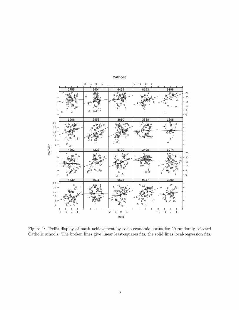
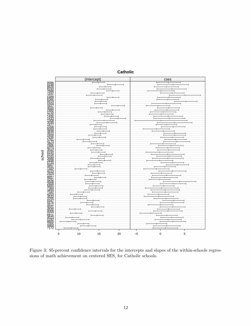
function has a method for objects of this class that returns by default 95-percent confidence intervalsfor the regression coefficients; the confidence intervals can be plotted, as follows:
> plot(intervals(cat.list), main="Catholic")
> plot(intervals(pub.list), main="Public")
The resulting graphs are shown in Figures 3 and 4. In interpreting these graphs, we need to becareful to take into account that we have not constrained the scales for the plots to be the same, andindeed the scales for the intercepts and slopes in the public schools are wider than in the Catholicschools. Because the SES variable is centered to 0 within schools, the intercepts are interpretable asthe average level of math achievement in each school. It is clear that there is substantial variationin the intercepts among both Catholic and public schools; the confidence intervals for the slopes,in contrast, overlap to a much greater extent, but there is still apparent school-to-school variation.
Parallel boxplots provide a different visualization of the estimated intercepts and slopes that iseasier to summarize. First, we save the coefficient estimates:
> cat.coef <- coef(cat.list)
> head(cat.coef, 6)
(Intercept) cses
7172 8.067 0.9945
4868 12.310 1.2865
2305 11.138 -0.7821
8800 7.336 2.5681
5192 10.409 1.6035
4523 8.352 2.3808
> pub.coef <- coef(pub.list)
> head(pub.coef, 6)
5A similar function is included in the lme4 package.
11
Catholic
scho
ol
7172486823058800519245236816227780094530902145116578934737053533425373423499736456502658950842928857131726294223146249315667572034983688816591048150404260741906399241735761763524583610383893592208147730391308143314362526275529903020342754045619636664697011733276888193862891989586
5 10 15 20
||
||
||
||
||
||
||
||
||
|||
||
||
||
||
||
||
||
||
||
||
||
||
||
||
||
||
||
||
||
|||
||
||
||
||
||
||
||
||
||
||
||
||
||
|||
||
||
||
||
||
||
||
||
||
||
||
||
||
||
||
||
||
||
||
|||
||
||
||
||
||
||
||
||
||
||
||
||
||
|||
||
||
|||
|||
||
||
||
||
||
||
||
||
||
||
||
||
||
||
||
||
||
|||
||
(Intercept)
−5 0 5
||
||
||
||
||
||
||
||
||
||
||
||
||
||
||
||
||
||
||
||
||
||
||
||
||
||
||
||
||
||
|||
||
||
||
|
||
||
||
||
||
||
||
|||
||
||
||
||
||
||
||
||
||
||
||
||
||
|||
||
||
||
||
||
||
||
||
||
||
||
||
||
||
||
||
||
||
||
||
||
||
||
||
||
||
||
||
||
||
|||
||
||
|||
||
||
||
||
||
||
||
||
||
||
||
||
cses
Figure 3: 95-percent confidence intervals for the intercepts and slopes of the within-schools regres-sions of math achievement on centered SES, for Catholic schools.
12

Public
scho
ol
836788544458576269905815734113584383308887757890614464436808281893405783301371012639337712964350939726559292898381884410870714998477128862911224396764159550646459377919371619092651246713746600388129955838915889467232291761702030835785314420399943256484689777348175887492255640608927685819639714611637194219462336262627713152333233513657464272767345769782028627
5 10 15 20
||
||
||
|||
||
||
||
||
||
||
||
||
||
||
||
||
|||
||
||
||
||
||
|||
||
||
||
||
|||
||
||
||
||
||
||
||
||
||
||
||
||
||
||
||
||
||
||
|||
||
||
||
||
||
||
||
||
||
||
||
||
||
||
||
||
||
||
||
||
||
||
||
||
||
||
||
||
||
||
||
||
||
||
||
||
||
||
||
||
|
||
||
||
||
|||
||
||
||
|||
||
||
||
||
||
||
||
||
||
||
||
||
|||
||
||
||
||
||
||
||
||
||
||
||
||
||
||
||
||
||
||
||
||
||
|(Intercept)
−5 0 5 10
||
||
||
||
||
||
||
||
|||
||
||
||
||
||
||||
||
||
||
||
||
||
||
||
||
||
||
||
||
||
||
||
||
||
||
||
||
||
||
||
||
||
||
||
|
||
||
||
||
||
||
||
||
||
||
||
||
||
||
||
|||
||
|||
|||
||
||
||
||
||
||
||
||
||
||
||
||
||
||
||
||
||
||
|||
||
||
||
||
||
||
|||
||
||
||
||
||
||
||
||
||
||
||
||
||
||
||
|||
||
||
||
||
||
||
||
||
||
||
||
||
||
||
||
||
|||
||
||
||
||
||
||
||
||
|cses
Figure 4: 95-percent confidence intervals for the intercepts and slopes of the within-schools regres-sions of math achievement on centered SES, for public schools.
13

Catholic Public
510
1520
Intercepts
Catholic Public
−2
02
46
Slopes
Figure 5: Boxplots of intercepts and slopes for the regressions of math achievement on centeredSES in Catholic and public schools..
(Intercept) cses
8367 4.553 0.2504
8854 4.240 1.9388
4458 5.811 1.1318
5762 4.325 -1.0141
6990 5.977 0.9477
5815 7.271 3.0180
The calls to coef extract matrices of regression coefficients from the lmList objects, with rowsrepresenting schools. Then, we draws separate plots for the intercepts and for the slopes:
> old <- par(mfrow=c(1, 2))
> boxplot(cat.coef[, 1], pub.coef[, 1], main="Intercepts",
+ names=c("Catholic", "Public"))
> boxplot(cat.coef[, 2], pub.coef[, 2], main="Slopes",
+ names=c("Catholic", "Public"))
> par(old) # restore
Setting the plotting parameter mfrow to 1 row and 2 columns produces the side-by-side pairs ofboxplots in Figure 5; mfrow is then returned to its previous value. The Catholic schools have ahigher average level of math achievement than the public schools, while the average slope relatingmath achievement to SES is larger in the public schools than in the Catholic schools.
2.1.3 Fitting a Hierarchical Linear Model with lme
Following Raudenbush and Bryk (2002) and Singer (1998), we will fit a hierarchical linear modelto the math-achievement data. This model consists of two sets of equations: First, within schools,
14

we have the regression of math achievement on the individual-level covariate SES; it aids inter-pretability of the regression coefficients to center SES at the school average; then the intercept foreach school estimates the average level of math achievement in the school. Using centered SES, theindividual-level equation for individual j in school i is
mathachij = α0i + α1icsesij + εij (2)
Second, at the school level, and also following Raudenbush, Bryk, and Singer, we will entertainthe possibility that the school intercepts and slopes depend upon sector and upon the average levelof SES in the schools:
α0i = γ00 + γ01meansesi + γ02sectori + u0i (3)
α1i = γ10 + γ11meansesi + γ12sectori + u1i
This kind of formulation is sometimes called a coefficients-as-outcomes model.6
Substituting the school-level Equations 3 into the individual-level Equation 2 produces
mathachij = γ00 + γ01meansesi + γ02sectori + u0i
+(γ10 + γ11meansesi + γ12sectori + u1j)csesij + εij
Rearranging terms,
mathachij = γ00 + γ01meansesi + γ02sectori + γ10csesij
+γ11meansesicsesij + γ12sectoricsesij
+u0i + u1icsesij + εij
Here, the γs are fixed effect coefficients, while the us (and the individual-level errors εij) are randomeffects.
Finally, rewriting the model in the notation of the LMM (Equation 1),
mathachij = β1 + β2meansesi + β3sectori + β4csesij (4)
+β5meansesicsesij + β6sectoricsesij
+bi1 + bi2csesij + εij
The change is purely notational, using βs for fixed effects and bs for random effects. (In the dataset, however, the school-level variables — that is, meanses and sector — are attached to theobservations for the individual students, as previously described.) We place no constraints on thecovariance matrix of the random effects7, so
Ψ = V
[bi1bi2
]=
[ψ21 ψ12
ψ12 ψ22
](5)
Also the individual-level errors are independent within schools, with constant variance:
V (εi) = σ2Ini
6This coefficients-as-outcomes model assumes that the regressions of the within-school intercepts and slopes onschool mean SES are linear. We invite the reader to examine this assumption by creating scatterplots of the within-school regression coefficients for Catholic and public schools, computed in the previous section, against school meanSES, modifying the hierarchical model in light of these graphs if the relationships appear nonlinear. For an analysisalong these lines, see the discussion of the High School and Beyond data in Fox (2016, Chap. 23).
7We are assuming, however, that the random effects for group i are independent of the random effects for anyother group i′.
15

Even though the individual-level errors are assumed to be independent, observations in the sameschool are correlated,
Var(mathachij) = σ2 + ψ21 + cses2ijψ
22 + 2csesijψ12
Cov(mathachij ,mathachij′) = ψ21 + csesijcsesij′ψ
22 + (csesij + csesij′)φ12
while observations in different groups are uncorrelated.As mentioned in Section 2, LMMs are fit with the lme function in the nlme package. Specifying
the fixed effects in the call to lme is identical to specifying a linear model in a call to lm (see Chapter4 of the text). Random effects are specified via the random argument to lme, which takes a one-sidedmodel formula.
Before fitting a mixed model to the math-achievement data, we reorder the levels of the factorsector so that the contrast for sector will use the value 0 for the public sector and 1 for theCatholic sector, in conformity with the coding employed by Raudenbush and Bryk (2002) and bySinger (1998):8
> Bryk$sector <- factor(Bryk$sector, levels=c("Public", "Catholic"))
> contrasts(Bryk$sector)
Catholic
Public 0
Catholic 1
Having established the contrast-coding for sector, the LMM in Equation 4 is fit as follows:
> bryk.lme.1 <- lme(mathach ~ meanses*cses + sector*cses,
+ random = ~ cses | school,
+ data=Bryk)
The formula for the random effects includes only the term for centered SES. As in a linear-modelformula, a random intercept is implied unless it is explicitly excluded (by specifying -1 in therandom formula). By default, lme fits the model by restricted maximum likelihood (REML), whichin effect corrects the maximum-likelihood estimator for degrees of freedom (see the complementaryreadings in Section 5).
> summary(bryk.lme.1)
Linear mixed-effects model fit by REML
Data: Bryk
AIC BIC logLik
46524 46592 -23252
Random effects:
Formula: ~cses | school
Structure: General positive-definite, Log-Cholesky parametrization
StdDev Corr
(Intercept) 1.5426 (Intr)
8Recoding changes the values of the fixed effects coefficient estimates but does not change other aspects of thefitted model.
16

cses 0.3182 0.391
Residual 6.0598
Fixed effects: mathach ~ meanses * cses + sector * cses
Value Std.Error DF t-value p-value
(Intercept) 12.128 0.1993 7022 60.86 0.0000
meanses 5.333 0.3692 157 14.45 0.0000
cses 2.945 0.1556 7022 18.93 0.0000
sectorCatholic 1.227 0.3063 157 4.00 0.0001
meanses:cses 1.039 0.2989 7022 3.48 0.0005
cses:sectorCatholic -1.643 0.2398 7022 -6.85 0.0000
Correlation:
(Intr) meanss cses sctrCt mnss:c
meanses 0.256
cses 0.075 0.019
sectorCatholic -0.699 -0.356 -0.053
meanses:cses 0.019 0.074 0.293 -0.026
cses:sectorCatholic -0.052 -0.027 -0.696 0.077 -0.351
Standardized Within-Group Residuals:
Min Q1 Med Q3 Max
-3.15926 -0.72319 0.01705 0.75445 2.95822
Number of Observations: 7185
Number of Groups: 160
The output from the summary method for lme objects consists of several panels:
� The first panel gives the AIC (Akaike information criterion) and BIC (Bayesian informationcriterion), which can be used for model selection (Fox and Weisberg, 2011, Section 4.5), alongwith the log of the maximized restricted likelihood.
� The next panel displays estimates of the variance and covariance parameters for the randomeffects, in the form of standard deviations and correlations. Thus, ψ̂1 = 1.543, ψ̂2 = 0.318,σ̂ = 6.060, and ψ̂12 = 0.391 × 1.543 × 0.318 = 0.192. The term labelled Residual is theestimate of σ.
� The table of fixed effects is similar to output from lm; to interpret the coefficients in thistable, refer to the hierarchical form of the model given in Equations 2 and 3, and to theLaird-Ware form of the LMM in Equation 4 (which orders the coefficients differently fromthe lme output). In particular, the fixed-effect intercept coefficient β̂1 = 12.128 represents anestimate of the average level of math achievement in public schools, which are the baselinecategory for the dummy regressor for sector. The remaining coefficient estimates could beinterpreted similarly to coefficients in a linear model. In particular, the apparent significanceof the interaction terms suggests that main effect terms should not be interpreted withoutconsidering the interactions. We prefer to do this interpretation using the effects plots thatwe will introduce shortly.
� The panel labelled Correlation gives the estimated sampling correlations among the fixed-effect coefficient estimates. These coefficient correlations are not usually of direct interest.
17

Very large correlations, however, are indicative of an ill-conditioned model — the analog ofhigh collinearity in a linear model.
� Some information about the standardized within-group residuals (ε̂ij/σ̂), the number of ob-servations, and the number of groups, appears at the end of the output.
The model we fit assumes that each school has its own slope and intercept sampled from abivariate normal distribution with covariance matrix Ψ given by Equation 5 (page 15). Testingif the elements of Ψ are 0 can be of interest in some problems. We can test hypotheses aboutthe variances and covariances of random effects by deleting random-effects terms from the model.Tests are based on the change in the log of the maximized restricted likelihood, calculating loglikelihood-ratio statistics. When LMMs are fit by REML, we must be careful, however, to comparemodels that are identical in their fixed effects.
For the current illustration, we may proceed as follows:
> bryk.lme.2 <- update(bryk.lme.1,
+ random = ~ 1 | school) # omitting random effect of cses
> anova(bryk.lme.1, bryk.lme.2)
Model df AIC BIC logLik Test L.Ratio p-value
bryk.lme.1 1 10 46524 46592 -23252
bryk.lme.2 2 8 46521 46576 -23252 1 vs 2 1.124 0.57
> bryk.lme.3 <- update(bryk.lme.1,
+ random = ~ cses - 1 | school) # omitting random intercept
> anova(bryk.lme.1, bryk.lme.3)
Model df AIC BIC logLik Test L.Ratio p-value
bryk.lme.1 1 10 46524 46592 -23252
bryk.lme.3 2 8 46740 46795 -23362 1 vs 2 220.6 <.0001
Each of these likelihood-ratio tests is on 2 degrees of freedom, because excluding one of the randomeffects removes not only its variance from the model but also its covariance with the other randomeffect. The large p-value in the first of these tests suggests no evidence of the need for a randomslope for centered SES, or equivalently that ψ12 = ψ2
2 = 0. The small p-value for the second testsuggests that ψ2
1 6= 0, and even accounting for differences due to sector and mean school SES, theaverage math achievement varies from school to school.
A more careful formulation of these tests takes account of the fact that each null hypothesisplaces a variance (but not covariance) component on a boundary of the parameter space. Con-sequently, the null distribution of the LR test statistic is not simply chisquare with 2 degrees offreedom, but rather a mixture of chisquare distributions.9 Moreover, it is reasonably simple tocompute the corrected p-value:
> pvalCorrected <- function(chisq, df){
+ (pchisq(chisq, df, lower.tail=FALSE) +
+ pchisq(chisq, df - 1, lower.tail=FALSE))/2
+ }
> pvalCorrected(1.124, df=2)
9See the complementary readings in Section 5 for discussion of this point.
18

[1] 0.4296
> pvalCorrected(220.6, df=2)
[1] 6.59e-49
Here, therefore, the corrected p-values are similar to the uncorrected ones.Model bryk.lme.2, fit above, omits the non-significant random effects for cses; the resulting
fixed-effects estimates are nearly identical to those for the initial model bryk.lme.1, which includesthese random effects:
> summary(bryk.lme.2)
Linear mixed-effects model fit by REML
Data: Bryk
AIC BIC logLik
46521 46576 -23252
Random effects:
Formula: ~1 | school
(Intercept) Residual
StdDev: 1.541 6.064
Fixed effects: mathach ~ meanses * cses + sector * cses
Value Std.Error DF t-value p-value
(Intercept) 12.128 0.1992 7022 60.88 0.0000
meanses 5.337 0.3690 157 14.46 0.0000
cses 2.942 0.1512 7022 19.46 0.0000
sectorCatholic 1.225 0.3061 157 4.00 0.0001
meanses:cses 1.044 0.2910 7022 3.59 0.0003
cses:sectorCatholic -1.642 0.2331 7022 -7.05 0.0000
Correlation:
(Intr) meanss cses sctrCt mnss:c
meanses 0.256
cses 0.000 0.000
sectorCatholic -0.699 -0.356 0.000
meanses:cses 0.000 0.000 0.295 0.000
cses:sectorCatholic 0.000 0.000 -0.696 0.000 -0.351
Standardized Within-Group Residuals:
Min Q1 Med Q3 Max
-3.17012 -0.72488 0.01485 0.75424 2.96551
Number of Observations: 7185
Number of Groups: 160
This model is sufficiently simple, despite the interactions, to interpret the fixed effects fromthe estimated coefficients, but even here it is likely easier to visualize the model in effect plots (asdiscussed for linear models in Fox and Weisberg, 2011, Section 4.3.3). Our effects package has
19
meanses*cses effect plot
cses
mat
hach
5
10
15
20
−3 −2 −1 0 1 2
meanses meanses
meanses
−3 −2 −1 0 1 2
5
10
15
20
meanses
cses*sector effect plot
csesm
atha
ch
5
10
15
−3 −2 −1 0 1 2
: sector Public
−3 −2 −1 0 1 2
: sector Catholic
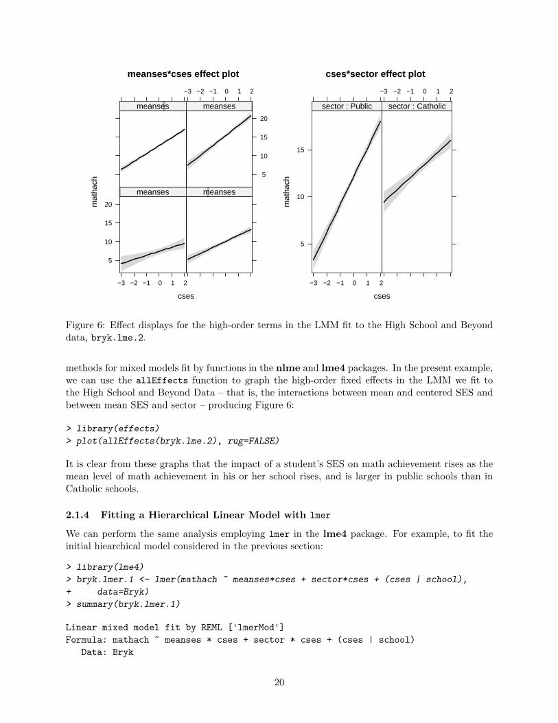
Figure 6: Effect displays for the high-order terms in the LMM fit to the High School and Beyonddata, bryk.lme.2.
methods for mixed models fit by functions in the nlme and lme4 packages. In the present example,we can use the allEffects function to graph the high-order fixed effects in the LMM we fit tothe High School and Beyond Data – that is, the interactions between mean and centered SES andbetween mean SES and sector – producing Figure 6:
> library(effects)
> plot(allEffects(bryk.lme.2), rug=FALSE)
It is clear from these graphs that the impact of a student’s SES on math achievement rises as themean level of math achievement in his or her school rises, and is larger in public schools than inCatholic schools.
2.1.4 Fitting a Hierarchical Linear Model with lmer
We can perform the same analysis employing lmer in the lme4 package. For example, to fit theinitial hiearchical model considered in the previous section:
> library(lme4)
> bryk.lmer.1 <- lmer(mathach ~ meanses*cses + sector*cses + (cses | school),
+ data=Bryk)
> summary(bryk.lmer.1)
Linear mixed model fit by REML ['lmerMod']
Formula: mathach ~ meanses * cses + sector * cses + (cses | school)
Data: Bryk
20

REML criterion at convergence: 46504
Scaled residuals:
Min 1Q Median 3Q Max
-3.159 -0.723 0.017 0.754 2.958
Random effects:
Groups Name Variance Std.Dev. Corr
school (Intercept) 2.380 1.543
cses 0.101 0.318 0.39
Residual 36.721 6.060
Number of obs: 7185, groups: school, 160
Fixed effects:
Estimate Std. Error t value
(Intercept) 12.128 0.199 60.9
meanses 5.333 0.369 14.4
cses 2.945 0.156 18.9
sectorCatholic 1.227 0.306 4.0
meanses:cses 1.039 0.299 3.5
cses:sectorCatholic -1.643 0.240 -6.9
Correlation of Fixed Effects:
(Intr) meanss cses sctrCt mnss:c
meanses 0.256
cses 0.075 0.019
sectorCthlc -0.699 -0.356 -0.053
meanses:css 0.019 0.074 0.293 -0.026
css:sctrCth -0.052 -0.027 -0.696 0.077 -0.351
The estimates of the fixed effects and variance/covariance components are the same as those ob-tained from lme (see page 16), but the specification of the model is slightly different: Rather thanusing a random argument as in lme, the random effects in lmer are given directly in the modelformula, enclosed in parentheses; as in lme, a random intercept is implied if it is not explicitlyremoved. An important difference between lme and lmer, however, is that lmer can accommodatecrossed random effects, while lme cannot: Suppose, for example, that we were interested in teachereffects on students’ achievement. Each student in a high school has several teachers, and so studentswould not be strictly nested within teachers.
A subtle difference between the lme and lmer output is that the former includes p-values forthe Wald t-tests of the estimated coefficients while the latter does not. The p-values in lmer aresuppressed because the Wald tests can be inaccurate. We address this issue in Section 2.2.
As in the previous section, let us proceed to remove the random slopes from the model, com-paring the resulting model to the initial model by a likelihood-ratio text:
> bryk.lmer.2 <- lmer(mathach ~ meanses*cses + sector*cses + (1 | school),
+ data=Bryk)
> anova(bryk.lmer.1, bryk.lmer.2)
21

refitting model(s) with ML (instead of REML)
Data: Bryk
Models:
bryk.lmer.2: mathach ~ meanses * cses + sector * cses + (1 | school)
bryk.lmer.1: mathach ~ meanses * cses + sector * cses + (cses | school)
Df AIC BIC logLik deviance Chisq Chi Df Pr(>Chisq)
bryk.lmer.2 8 46513 46568 -23249 46497
bryk.lmer.1 10 46516 46585 -23248 46496 1 2 0.61
Out of an abundance of caution, anova refits the models using ML rather than REML, becauseLR tests of models fit by REML that differ in their fixed effects are inappropriate. In our case,however, the models compared have identical fixed effects and differ only in the random effects. Alikelihood-ratio test is therefore appropriate even if the models are fit by REML. We can obtainthis test by specifying the argument refit=FALSE:
> anova(bryk.lmer.1, bryk.lmer.2, refit=FALSE)
Data: Bryk
Models:
bryk.lmer.2: mathach ~ meanses * cses + sector * cses + (1 | school)
bryk.lmer.1: mathach ~ meanses * cses + sector * cses + (cses | school)
Df AIC BIC logLik deviance Chisq Chi Df Pr(>Chisq)
bryk.lmer.2 8 46521 46576 -23252 46505
bryk.lmer.1 10 46524 46592 -23252 46504 1.12 2 0.57
The results are identical to those using lme.
2.2 Wald Tests for Linear Mixed Models
As we mentioned, it is inappropriate to perform likelihood-ratio tests for fixed effects when a LMMis fit by REML. Though it is sometimes recommended that ML be used instead to obtain LR testsof fixed effects, ML estimates can be substantially biased when there are relatively few higher-levelunits. Wald tests can be performed, however, for the fixed effects in a LMM estimated by REML,but as we also mentioned, Wald tests obtained for individual coefficients by dividing estimated fixedeffects by their standard errors can be inaccurate. The same is true of more complex Wald testson several degrees of freedom — for example, F -tests for terms in a linear mixed model.
One approach to obtaining more accurate inferences in LMMs fit by REML is to adjust theestimated covariance matrix of the fixed effects to reduce the typically downward bias of the coeffi-cient standard errors, as suggested by Kenward and Roger (1997), and to adjust degrees of freedomfor t and F tests (applying a method introduced by Satterthwaite, 1946). These adjustments areavailable for linear mixed models fit by lmer in the Anova and linearHypothesis functions in thecar package, employing infrastructure from the pbkrtest package. For example,
> library(car)
> Anova(bryk.lmer.2, test="F")
Analysis of Deviance Table (Type II Wald F tests with Kenward-Roger df)
Response: mathach
F Df Df.res Pr(>F)
22

meanses 209.2 1 156 < 2e-16
cses 409.4 1 7023 < 2e-16
sector 16.0 1 154 9.8e-05
meanses:cses 12.9 1 7023 0.00033
cses:sector 49.6 1 7023 2.0e-12
In this case, with many schools and a moderate number of students within each school, the KRtests are essentially the same as Wald chisquare tests using the naively computed covariance matrixfor the fixed effects:
> Anova(bryk.lmer.2)
Analysis of Deviance Table (Type II Wald chisquare tests)
Response: mathach
Chisq Df Pr(>Chisq)
meanses 209.2 1 < 2e-16
cses 409.4 1 < 2e-16
sector 16.0 1 6.3e-05
meanses:cses 12.9 1 0.00033
cses:sector 49.6 1 1.9e-12
2.3 Examining the Random Effects: Computing BLUPs
The model bryk.lmer.2 includes a random intercept for each school. A natural question to ask inthis problem is which schools have the largest intercepts, as these would be the highest achievingschools, and which schools have the smallest intercepts, as these are the schools that have thelowest math achievement. The model is given by Equation 4 (on page 15), with bi2 = 0, and so theintercept for the ith school is β1 + bi1 for public schools and β1 + bi1 + β3 for Catholic schools. Ineither case bi1 represents the difference between the mean for the i-th school and the mean for thatschool’s sector.
Estimates for the intercept β1 and for β3 can be obtained from the summary output shownpreviously, and can be retrieved from the fitted model with
> fixef(bryk.lmer.2)
(Intercept) meanses cses sectorCatholic
12.128 5.337 2.942 1.225
meanses:cses cses:sectorCatholic
1.044 -1.642
The bi1 are random variables that are not directly estimated from the fitted model. Rather, lme4computes the mode of the conditional distribution of each bi1 given the fitted model as predictionsof the bi1. Here are the first 6 of them:
> school.effects <- ranef(bryk.lmer.2)$school
> head(school.effects, 6)
(Intercept)
8367 -3.6626
23

8854 -2.5948
4458 -0.5416
5762 -1.0094
6990 -2.7383
5815 -0.7584
Such “estimated” random effects (with “estimated” in quotes because the random-effect coefficientsare random variables, not parameters) are often called best linear unbiased predictors or BLUPs.
The ranef function is very complicated because it needs to be able to accomodate complexmodels with one or more levels of hierarchy, and with one or more random effect per level in thehierarchy. The command ranef(bryk.lmer.2)$school returns the random effects for schools as amatrix with one column.
To judge the size of the school random effects, the standard deviation of mathach for all studentsis about 7 units, and the average number of students per school is about 45, so the standard error ofschool average achievement is about 7/
√45 ≈ 1. A school intercept random effect of 2, for example,
correponds to 2 standard deviations above average, and −2 is 2 standard deviations below average.Because the random effects are assumed to be normally distributed, we should expect to find fewrandom effects predicted to be larger than about 3 or smaller than about −3.
The bottom and top 5 performing Catholic Schools can be identified as follows:
> cat <- MathAchSchool$Sector == "Catholic" # TRUE for Catholic, FALSE for Public
> cat.school.effects <- school.effects[cat, 1, drop=FALSE]
> or <- order(cat.school.effects[, 1]) # order school effects
> cat.school.effects[or, , drop=FALSE][c(1:5, 66:70), , drop=FALSE]
(Intercept)
6990 -2.738
4868 -2.041
9397 -1.872
6808 -1.723
2658 -1.709
4292 1.701
2629 1.801
8193 2.810
8628 3.128
3427 4.215
The argument drop=FALSE is used in several places to force R to keep a one-column matrix as amatrix to preserve the row names, corresponding to school numbers. For public schools, we get
> pub.school.effects <- school.effects[!cat, 1, drop=FALSE]
> or <- order(pub.school.effects[, 1]) # order the school effects for Catholic Schools
> pub.school.effects[or, , drop=FALSE][c(1:5, 86:90), , drop=FALSE]
(Intercept)
8367 -3.663
4523 -3.546
3705 -3.180
7172 -2.766
24

8854 -2.595
6089 2.030
9198 2.077
6170 2.109
2655 3.053
7688 3.169
Possibly apart from school 6990, there were no extremely poorly performing Catholic schools, whilethere seem to be 2 or 3 highly performing schools. The public schools include a few very poorlyperforming schools and 2 highly performing schools.
2.4 An Illustrative Application to Longitudinal Data
To illustrate the use of linear mixed models in longitudinal research, we draw on data described byDavis et al. (2005) on the exercise histories of 138 teenaged girls hospitalized for eating disordersand of 93 comparable “control” subjects.10 The data are in the data frame Blackmore in the carpackage:
> head(Blackmore, 20)
subject age exercise group
1 100 8.00 2.71 patient
2 100 10.00 1.94 patient
3 100 12.00 2.36 patient
4 100 14.00 1.54 patient
5 100 15.92 8.63 patient
6 101 8.00 0.14 patient
7 101 10.00 0.14 patient
8 101 12.00 0.00 patient
9 101 14.00 0.00 patient
10 101 16.67 5.08 patient
11 102 8.00 0.92 patient
12 102 10.00 1.82 patient
13 102 12.00 4.75 patient
15 102 15.08 24.72 patient
16 103 8.00 1.04 patient
17 103 10.00 2.90 patient
18 103 12.00 2.65 patient
20 103 14.08 6.86 patient
21 104 8.00 2.75 patient
22 104 10.00 6.62 patient
The variables are:
� subject: an identification code; there are several observations for each subject, but becausethe girls were hospitalized at different ages, the number of observations and the age at thelast observation vary.
10These data were generously made available to us by Elizabeth Blackmore and Caroline Davis of York University.
25

� age: the subject’s age in years at the time of observation; all but the last observation for eachsubject were collected retrospectively at intervals of 2 years, starting at age 8.
� exercise: the amount of exercise in which the subject engaged, expressed as estimated hoursper week.
� group: a factor indicating whether the subject is a "patient" or a "control".11
2.4.1 Examining the Data
Initial examination of the data suggested that it is advantageous to take the log of exercise: Doingso makes the exercise distribution for both groups of subjects more symmetric and linearizes therelationship of exercise to age.12 Because there are some 0 values of exercise, we use “started”logs in the analysis reported below (transformations are discussed in Fox and Weisberg, 2011,Section 3.4), adding 5 minutes (5/60 of an hour) to each value of exercise prior to taking logs(and using logs to the base 2 for interpretability):
> Blackmore$log.exercise <- log2(Blackmore$exercise + 5/60)
As in the analysis of the math-achievement data in the preceding section, we begin by sampling20 subjects from each of the patient and control groups, plotting log.exercise against age foreach subject:
> pat <- with(Blackmore, sample(unique(subject[group == "patient"]), 20))
> Pat.20 <- groupedData(log.exercise ~ age | subject,
+ data=Blackmore[is.element(Blackmore$subject, pat),])
> con <- with(Blackmore, sample(unique(subject[group == "control"]), 20))
> Con.20 <- groupedData(log.exercise ~ age | subject,
+ data=Blackmore[is.element(Blackmore$subject, con),])
> print(plot(Con.20, main="Control Subjects",
+ xlab="Age", ylab="log2 Exercise",
+ ylim=1.2*range(Con.20$log.exercise, Pat.20$log.exercise),
+ layout=c(5, 4), aspect=1.0),
+ position=c(0, 0, 0.5, 1), more=TRUE)
> print(plot(Pat.20, main="Patients",
+ xlab="Age", ylab="log2 Exercise",
+ ylim=1.2*range(Con.20$log.exercise, Pat.20$log.exercise),
+ layout=c(5, 4), aspect=1.0),
+ position=c(0.5, 0, 1, 1))
The graphs appear in Figure 7.
� Each Lattice plot is constructed by using the default plot method for grouped-data objects.Grouped-data objects, provided by the nlme package, are enhanced data frames, incorporat-ing a model formula that gives information about the structure of the data. In this instance,the formula log.exercise ~ age | subject, read as “log.exercise depends on age given
11To avoid the possibility of confusion, we point out that the variable group represents groups of independentpatients and control subjects, and is not a factor defining clusters. Clusters in this longitudinal data set are definedby the variable subject.
12We invite the reader to examine the distribution of the exercise variable, before and after log-transformation.
26

Control Subjects
Age
log2
Exe
rcis
e
−4−2
024
8 12 16
254 266
8 12 16
264 201
8 12 16
206
275 246 245 273b
−4−2024
226−4−2
024
255 205 207a 228 269
220
8 12 16
200 238
8 12 16
212
−4−2024
241
Patients
Age
log2
Exe
rcis
e
−4−2
024
8 12 16
338 179
8 12 16
162 326
8 12 16
118
189 306 177 329
−4−2024
136−4−2
024
165 106 335 143 305
148
8 12 16
119 129
8 12 16
321
−4−2024
180
Figure 7: log2 exercise by age for 20 randomly selected patients and 20 randomly selected controlsubjects.
27

subject,” indicates that log.exercise is the response variable, age is the principal within-subject covariate (actually, in this application, it is the only within-subject covariate), andthe data are grouped by subject.
� To make the two plots comparable, we have exerted direct control over the scale of the verticalaxis (set to slightly larger than the range of the combined log-exercise values), the layout ofthe plot (5 columns, 4 rows),13 and the aspect ratio of the plot (the ratio of the vertical tothe horizontal size of the plotting region in each panel, set here to 1.0).
� The print method for Lattice objects, normally automatically invoked when the returnedobject is not assigned to a variable, simply plots the object on the active graphics device. Soas to print both plots on the same “page,” we have instead called print explicitly, using theposition argument to place each graph on the page. The form of this argument is c(xmin,
ymin, xmax, ymax), with horizontal (x) and vertical (y) coordinates running from 0, 0 (thelower-left corner of the page) to 1, 1 (the upper-right corner). The argument more=TRUE inthe first call to print indicates that the graphics page is not yet complete.
There are few observations for each subject, and in many instances, no strong within-subjectpattern. Nevertheless, it appears as if the general level of exercise is higher among the patientsthan among the controls. As well, the trend for exercise to increase with age appears stronger andmore consistent for the patients than for the controls.
We pursue these impressions by fitting regressions of log.exercise on age for each subject.Because of the small number of observations per subject, we should not expect very good estimatesof the within-subject regression coefficients. Indeed, one of the advantages of mixed models is thatthey can provide improved estimates of the within-subject coefficients (the random effects plus thefixed effects) by pooling information across subjects.14
> pat.list <- lmList(log.exercise ~ I(age - 8) | subject,
+ subset = group=="patient", data=Blackmore)
> con.list <- lmList(log.exercise ~ I(age - 8) | subject,
+ subset = group=="control", data=Blackmore)
> pat.coef <- coef(pat.list)
> con.coef <- coef(con.list)
> old <- par(mfrow=c(1, 2))
> boxplot(pat.coef[,1], con.coef[,1], main="Intercepts",
+ names=c("Patients", "Controls"))
> boxplot(pat.coef[,2], con.coef[,2], main="Slopes",
+ names=c("Patients", "Controls"))
> par(old)
Boxplots of the within-subjects regression coefficients are shown in Figure 8. We changed the originof age to 8 years, which is the initial observation for each subject, so the intercept represents levelof exercise at the start of the study. As expected, there is a great deal of variation in both theintercepts and the slopes. The median intercepts are similar for patients and controls, but there issomewhat more variation among patients. The slopes are higher on average for patients than forcontrols, for whom the median slope is close to 0.
13Notice the unusual ordering in specifying the layout — columns first, then rows.14Pooled estimates of the random effects provide so-called best-linear-unbiased predictors (or BLUPs) of the regres-
sion coefficients for individual subjects. See help(predict.lme), Section 2.3, and the complementary readings.
28

Patients Controls
−4
−2
02
Intercepts
Patients Controls
−1.
0−
0.5
0.0
0.5
1.0
Slopes
Figure 8: Coefficients for the within-subject regressions of log2 exercise on age, for patients andcontrol subjects.
29

2.4.2 Fitting a Mixed Model with Autocorrelated Errors
We proceed to fit a LMM to the data, including fixed effects for age (again, with an origin of 8),group, and their interaction, and random intercepts and slopes:
> bm.lme.1 <- lme(log.exercise ~ I(age - 8)*group,
+ random = ~ I(age - 8) | subject, data=Blackmore)
> summary(bm.lme.1)
Linear mixed-effects model fit by REML
Data: Blackmore
AIC BIC logLik
3630 3669 -1807
Random effects:
Formula: ~I(age - 8) | subject
Structure: General positive-definite, Log-Cholesky parametrization
StdDev Corr
(Intercept) 1.4436 (Intr)
I(age - 8) 0.1648 -0.281
Residual 1.2441
Fixed effects: log.exercise ~ I(age - 8) * group
Value Std.Error DF t-value p-value
(Intercept) -0.2760 0.18237 712 -1.514 0.1306
I(age - 8) 0.0640 0.03136 712 2.041 0.0416
grouppatient -0.3540 0.23529 229 -1.504 0.1338
I(age - 8):grouppatient 0.2399 0.03941 712 6.087 0.0000
Correlation:
(Intr) I(g-8) grpptn
I(age - 8) -0.489
grouppatient -0.775 0.379
I(age - 8):grouppatient 0.389 -0.796 -0.489
Standardized Within-Group Residuals:
Min Q1 Med Q3 Max
-2.7349 -0.4245 0.1228 0.5280 2.6362
Number of Observations: 945
Number of Groups: 231
Examining the naive t-tests for the fixed effects, we start as usual with the test for the interactions,and in this case the interaction of age with group is highly significant, reflecting a much steeperaverage trend in the patient group. In light of the interaction, tests for the main effects of age andgroup are not of interest.15
15The pbkrtest package will not provide corrected standard errors and degrees of freedom for models fit by lme
(as opposed to lmer).
30

We turn next to the random effects, and test whether the random intercepts and slopes are nec-essary, omitting each in turn from the model and calculating a likelihood-ratio statistic, contrastingthe refitted model with the original model:
> bm.lme.2 <- update(bm.lme.1, random = ~ 1 | subject)
> anova(bm.lme.1, bm.lme.2) # test for random slopes
Model df AIC BIC logLik Test L.Ratio p-value
bm.lme.1 1 8 3630 3669 -1807
bm.lme.2 2 6 3644 3673 -1816 1 vs 2 18.12 0.0001
> bm.lme.3 <- update(bm.lme.1, random = ~ I(age - 8) - 1 | subject)
> anova(bm.lme.1, bm.lme.3) # test for random intercepts
Model df AIC BIC logLik Test L.Ratio p-value
bm.lme.1 1 8 3630 3669 -1807
bm.lme.3 2 6 3834 3863 -1911 1 vs 2 207.9 <.0001
The tests are highly statistically significant, suggesting that both random intercepts and randomslopes are required.
Let us next consider the possibility that the within-subject errors (the εijs in the mixed modelof Equation 1 on page 2) are autocorrelated, as may well be the case, because the observationsare taken longitudinally on the same subjects. The lme function incorporates a flexible mecha-nism for specifying error-correlation structures, and supplies constructor functions for several suchstructures.16 Most of these correlation structures, however, are appropriate only for equally spacedobservations. An exception is the corCAR1 function, which permits us to fit a continuous first-orderautoregressive process in the errors. Suppose that εit and εi,t+s are errors for subject i separatedby s units of time, where s need not be an integer; then, according to the continuous first-orderautoregressive model, the correlation between these two errors is ρ(s) = φ|s| where 0 ≤ φ < 1.This appears a reasonable specification in the current context, where there are at most ni = 5observations per subject.
Fitting the model with CAR1 errors to the data produces a convergence failure:
> bm.lme.4 <- update(bm.lme.1, correlation = corCAR1(form = ~ age | subject))
Error in lme.formula(fixed = log.exercise ~ I(age - 8) * group, data = Blackmore, :
nlminb problem, convergence error code = 1
message = iteration limit reached without convergence (10)
The correlation structure is given in the correlation argument to lme (here as a call to corCAR1);the form argument to corCAR1 is a one-sided formula defining the time dimension (here, age) andthe group structure (subject). With so few observations within each subject, it is difficult to sepa-rate the estimated correlation of the errors from the correlations among the observations induced byclustering, as captured by subject-varying intercepts and slopes. This kind of convergence problemis a common occurrence in mixed-effects modeling.
We will therefore fit two additional models to the data, each including either random interceptsor random slopes (but not both) along with autocorrelated errors:
16A similar mechanism is provided for modeling non-constant error variance, via the weights argument to lme. Seethe documentation for lme for details. In contrast, the lmer function in the lme4 package does not accommodateautocorrelated errors, which is why we used lme for this example.
31

> bm.lme.5 <- update(bm.lme.1, random = ~ 1 | subject,
+ correlation = corCAR1(form = ~ age |subject)) # random intercepts (not slopes)
> bm.lme.6 <- update(bm.lme.1, random = ~ I(age - 8) - 1 | subject,
+ correlation = corCAR1(form = ~ age |subject)) # random slopes (not intercepts)
These models and our initial model without autocorrelated errors (bm.lme.1) are not properlynested for likelihood-ratio tests — indeed bm.lme.5 and bm.lme6 have the same number of param-eters — but we can examine the maximimzed restricted log-likilihood under the models along withthe AIC and BIC model-selection criteria:
> table <- matrix(0, 3, 3)
> table[, 1] <- c(logLik(bm.lme.1), logLik(bm.lme.5), logLik(bm.lme.6))
> table[, 2] <- c(BIC(bm.lme.1), BIC(bm.lme.5), BIC(bm.lme.6))
> table[, 3] <- c(AIC(bm.lme.1), AIC(bm.lme.5), AIC(bm.lme.6))
> colnames(table) <- c("logLik", "BIC", "AIC")
> rownames(table) <- c("bm.lme.1", "bm.lme.5", "bm.lme.6")
> table
logLik BIC AIC
bm.lme.1 -1807 3669 3630
bm.lme.5 -1795 3639 3605
bm.lme.6 -1803 3654 3620
All of these criteria point to model bm.lme.5, with random intercepts, a fixed age slope (withinpatient/control groups), and autocorrelated errors.
Although we expended some effort in modeling the random effects, the estimates of the fixedeffects, and their standard errors, do not depend critically on the random-effect specification of themodel, also a common occurrence:
> compareCoefs(bm.lme.1, bm.lme.5, bm.lme.6)
Call:
1: lme.formula(fixed = log.exercise ~ I(age - 8) * group, data = Blackmore,
random = ~I(age - 8) | subject)
2: lme.formula(fixed = log.exercise ~ I(age - 8) * group, data = Blackmore,
random = ~1 | subject, correlation = corCAR1(form = ~age | subject))
3: lme.formula(fixed = log.exercise ~ I(age - 8) * group, data = Blackmore,
random = ~I(age - 8) - 1 | subject, correlation = corCAR1(form = ~age |
subject))
Est. 1 SE 1 Est. 2 SE 2 Est. 3 SE 3
(Intercept) -0.2760 0.1824 -0.3070 0.1895 -0.3178 0.1935
I(age - 8) 0.0640 0.0314 0.0728 0.0317 0.0742 0.0365
grouppatient -0.3540 0.2353 -0.2838 0.2447 -0.2487 0.2500
I(age - 8):grouppatient 0.2399 0.0394 0.2274 0.0397 0.2264 0.0460
The summary for model bm.lme.5 is as follows:
> summary(bm.lme.5)
32

Linear mixed-effects model fit by REML
Data: Blackmore
AIC BIC logLik
3605 3639 -1795
Random effects:
Formula: ~1 | subject
(Intercept) Residual
StdDev: 1.15 1.529
Correlation Structure: Continuous AR(1)
Formula: ~age | subject
Parameter estimate(s):
Phi
0.6312
Fixed effects: log.exercise ~ I(age - 8) * group
Value Std.Error DF t-value p-value
(Intercept) -0.30697 0.18950 712 -1.620 0.1057
I(age - 8) 0.07278 0.03168 712 2.297 0.0219
grouppatient -0.28383 0.24467 229 -1.160 0.2472
I(age - 8):grouppatient 0.22744 0.03974 712 5.723 0.0000
Correlation:
(Intr) I(g-8) grpptn
I(age - 8) -0.553
grouppatient -0.775 0.428
I(age - 8):grouppatient 0.441 -0.797 -0.556
Standardized Within-Group Residuals:
Min Q1 Med Q3 Max
-2.9431 -0.4640 0.1732 0.5869 2.0220
Number of Observations: 945
Number of Groups: 231
There is, therefore, a moderately large estimated error autocorrelation, φ̂ = .631.To get a more concrete sense of the fixed effects, using model bm.lme.5 (which includes auto-
correlated errors and random intercepts, but not random slopes), we employ the predict methodfor lme objects to calculate fitted values for patients and controls across the range of ages (8 to 18)represented in the data:
> pdata <- expand.grid(age=seq(8, 18, by=2), group=c("patient", "control"))
> pdata$log.exercise <- predict(bm.lme.5, pdata, level=0)
> pdata$exercise <- 2^pdata$log.exercise - 5/60
> pdata
age group log.exercise exercise
1 8 patient -0.590801 0.5806
2 10 patient 0.009641 0.9234
3 12 patient 0.610082 1.4430
33

8 10 12 14 16 18
12
34
5
Age (years)
Exe
rcis
e (h
ours
/wee
k)
PatientsControls
Figure 9: Fitted values representing estimated fixed effects of group, age, and their interaction.
4 14 patient 1.210523 2.2309
5 16 patient 1.810964 3.4254
6 18 patient 2.411405 5.2366
7 8 control -0.306970 0.7250
8 10 control -0.161409 0.8108
9 12 control -0.015847 0.9057
10 14 control 0.129715 1.0107
11 16 control 0.275277 1.1269
12 18 control 0.420838 1.2554
Specifying level=0 in the call to predict produces estimates of the fixed effects. The expression2^pdata$log.exercise - 5/60 translates the fitted values of exercise from the log2 scale back tohours/week.
Finally, we plot the fitted values (Figure 9):
> plot(pdata$age, pdata$exercise, type="n",
+ xlab="Age (years)", ylab="Exercise (hours/week)")
> points(pdata$age[1:6], pdata$exercise[1:6], type="b", pch=19, lwd=2)
> points(pdata$age[7:12], pdata$exercise[7:12], type="b", pch=22, lty=2, lwd=2)
> legend("topleft", c("Patients", "Controls"), pch=c(19, 22),
+ lty=c(1,2), lwd=2, inset=0.05)
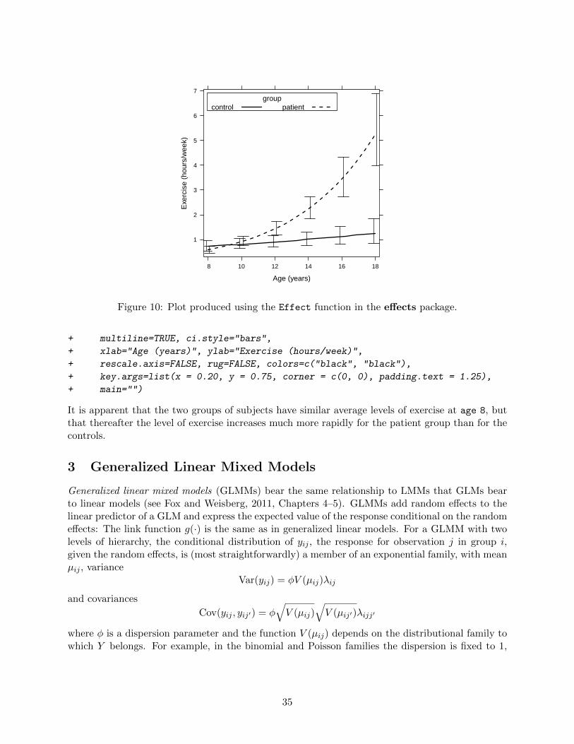
Essentially the same graph (Figure 10) can be constructed by the effects package, with the addedfeature of confidence intervals for the estimated effects:
> plot(Effect(c("age", "group"), bm.lme.5, xlevels=list(age=seq(8, 18, by=2)),
+ transformation=list(link=function(x) log2(x + 5/60),
+ inverse=function(x) 2^x - 5/60)),
34
Age (years)
Exe
rcis
e (h
ours
/wee
k)
1
2
3
4
5
6
7
8 10 12 14 16 18
groupcontrol patient
Figure 10: Plot produced using the Effect function in the effects package.
+ multiline=TRUE, ci.style="bars",
+ xlab="Age (years)", ylab="Exercise (hours/week)",
+ rescale.axis=FALSE, rug=FALSE, colors=c("black", "black"),
+ key.args=list(x = 0.20, y = 0.75, corner = c(0, 0), padding.text = 1.25),
+ main="")
It is apparent that the two groups of subjects have similar average levels of exercise at age 8, butthat thereafter the level of exercise increases much more rapidly for the patient group than for thecontrols.
3 Generalized Linear Mixed Models
Generalized linear mixed models (GLMMs) bear the same relationship to LMMs that GLMs bearto linear models (see Fox and Weisberg, 2011, Chapters 4–5). GLMMs add random effects to thelinear predictor of a GLM and express the expected value of the response conditional on the randomeffects: The link function g(·) is the same as in generalized linear models. For a GLMM with twolevels of hierarchy, the conditional distribution of yij , the response for observation j in group i,given the random effects, is (most straightforwardly) a member of an exponential family, with meanµij , variance
Var(yij) = φV (µij)λij
and covariances
Cov(yij , yij′) = φ√V (µij)
√V (µij′)λijj′
where φ is a dispersion parameter and the function V (µij) depends on the distributional family towhich Y belongs. For example, in the binomial and Poisson families the dispersion is fixed to 1,
35

and in the Gaussian family V (µ) = 1. Alternatively, for quasi-likelihood estimation, V (·) can begiven directly.17
The GLMM may therefore be written as
ηij = β1 + β2x2ij + · · ·+ βpxpij + b1iz1ij + · · ·+ bqizqij
g(µij) = E(yij |b1i, . . . , bqi) = ηij
bki ∼ N(0, ψ2k),Cov(bki, bk′i) = ψkk′
bki, bk′i′ are independent for i 6= i′
Var(yij) = φV (µij)λij
Cov(yij , yij′) = φ√V (µij)
√V (µij′)λijj′
yij , yij′ are independent for i 6= i′
where ηij is the linear predictor for observation j in cluster i; the fixed-effect coefficients (βs),random-effect coefficients (bs), fixed-effect regressors (xs), and random-effect regressors (zs) aredefined as in the LMM.18
In matrix form, the GLMM is
ηi = Xiβ + Zibi (6)
g(µi) = g[E(yi|bi)] = ηi
bi ∼ Nq(0,Ψ)
bi,bi′ are independent for i 6= i′
E(yi|bi) = µi (7)
V (yi|bi) = φV 1/2(µi)ΛiV1/2(µi) (8)
yi,yi′ are independent for i 6= i′
where
� yi is the ni × 1 response vector for observations in the ith of m groups;
� µi is the ni × 1 expectation vector for the response, conditional on the random effects;
� ηi is the ni × 1 linear predictor for the elements of the response vector;
� g(·) is the link function, transforming the conditional expected response to the linear predictor;
� Xi is the ni × p model matrix for the fixed effects of observations in group i;
� β is the p× 1 vector of fixed-effect coefficients;
� Zi is the ni × q model matrix for the random effects of observations in group i;
� bi is the q × 1 vector of random-effect coefficients for group i;
� Ψ is the q × q covariance matrix of the random effects;
� Λi is ni × ni and expresses the dependence structure for the conditional distribution of theresponse within each group—for example, if the observations are sampled independently ineach group, Λi = Ini ;
19
17As in the generalized linear model (Fox and Weisberg, 2011, Section 10.5.3).18 The glmer function in the lme4 package that we will use to fit GLMMs is somewhat more restrictive, setting
λkk = 1 and λkk′ = 0.19As mentioned, this restriction is imposed by the glmer function in the lme4 package. See footnote 18.
36

� V 1/2(µi) ≡ diag[√V (µij)]; and
� φ is the dispersion parameter.
3.1 Example: Migraine Headaches
In an effort to reduce the severity and frequency of migraine headaches through the use of biofeed-back training, Tammy Kostecki-Dillon collected longitudinal data on migraine-headache sufferers.20
The 133 patients who participated in the study were each given four weekly sessions of biofeedbacktraining. The patients were asked to keep daily logs of their headaches for a period of 30 days priorto training, during training, and post-training, to 100 days after training began. Compliance withthese instructions was low, and there is therefore quite a bit of missing data; for example, only 55patients kept a log prior to training. On average, subjects recorded information on 31 days, withthe number of days ranging from 7 to 121. Subjects were divided into three self-selected groups:those who discontinued their migraine medication during the training and post-training phase ofthe study; those who continued their medication, but at a reduced dose; and those who continuedtheir medication at the previous dose.
We will use a binomial GLMM—specifically, a binary logit mixed-effects model—to analyze theincidence of headaches during the period of the study. Examination of the data suggested thatthe incidence of headaches was constant during the pre-training phase of the study, increased, aswas expected by the investigator, at the start of training, and then declined at a decreasing rate.We decided to fit a linear trend prior to the start of training (before time 0), possibly to capturea trend that we failed to detect in our exploration of the data; and to transform time at day 1and later (which, for simplicity, we term “time post-treatment”) by taking the square-root.21 Inaddition to the intercept, representing the level of headache incidence at the end of the pre-trainingperiod, we include a dummy regressor coded 1 post-treatment, and 0 pre-treatment, to capture theanticipated increase in headache incidence at the start of training; dummy regressors for levels ofmedication; and interactions between medication and treatment, and between medication and thepre- and post-treatment time trends. Thus, the fixed-effects part of the model is
logit(µij) = β1 + β2m1i + β3m2i + β4pij + β5t0ij + β6√t1ij
+ β7m1ipij + β8m2ipij + β9m1it0ij + β10m2it0ij
+ β11m1i
√t1ij + β12m2i
√t1ij
where
� µij is the probability of a headache for individual i = 1, . . . , 133, on occasion j = 1, . . . , ni,conditional on the random effects;
� m1i and m2i are the dummy regressors for a factor medication with levels none, reducedand continuing for no medication, reduced medication, and no change in medication;
� pij is a dummy regressor for a factor treatment with levels no and yes;
� t0ij is time (in days) pre-treatment in a variable pretime, running from −29 through 0, andcoded 0 after treatment began; and
20The data are described by Kostecki-Dillon, Monette, and Wong (1999) and were generously made available byGeorges Monette, who performed the original data analysis. The analysis reported here is similar to his.
21The original analysis of the data by Georges Monette used regression splines for time-trends, with results generallysimilar to those reported here.
37

� t1ij is time (in days) post-treatment in a variable posttime, running from 1 through 99, andcoded 0 pre-treatment.
This specification for the fixed-effects can be summarized in the matrix X with 12 columns corre-ponding to the regressors multipying each of the 12 βs in the fixed-effects part of the model.
For random effects, we allow a separate random intercept for pre- and post-treatment by in-cluding both the intercept and treatment among the random effects. In addition, we allow randomslopes for both pretreat and posttreat. The matrix Z will have 4 columns, and the correspond-ing coviarance matrix Ψ has 4 variance terms and 6 covariance terms for a total of 10 parameters,complexity that can cause numerical problems as we will see shortly.
The data for this example are in the KosteckiDillon data frame in the car package. We beginwith a bit of data-management to compute the variables needed from those already in the data set:
> KosteckiDillon$treatment <- factor(with(KosteckiDillon,
+ ifelse(time > 0, "yes", "no")))
> KosteckiDillon$pretreat <- with(KosteckiDillon, ifelse(time > 0, 0, time))
> KosteckiDillon$posttreat <- with(KosteckiDillon, ifelse(time > 0, time, 0))
> head(KosteckiDillon, 10)
id time dos hatype age airq medication headache sex treatment pretreat
1 1 -11 753 Aura 30 9 continuing yes female no -11
2 1 -10 754 Aura 30 7 continuing yes female no -10
3 1 -9 755 Aura 30 10 continuing yes female no -9
4 1 -8 756 Aura 30 13 continuing yes female no -8
5 1 -7 757 Aura 30 18 continuing yes female no -7
6 1 -6 758 Aura 30 19 continuing yes female no -6
7 1 -5 759 Aura 30 17 continuing yes female no -5
8 1 22 786 Aura 30 21 continuing yes female yes 0
9 1 23 787 Aura 30 21 continuing yes female yes 0
10 1 24 788 Aura 30 18 continuing yes female yes 0
posttreat
1 0
2 0
3 0
4 0
5 0
6 0
7 0
8 22
9 23
10 24
There are variables in the data set that we will not use in the example in this section; for details,see ?KosteckiDillon.
GLMMs may be fit by the glmer function (pronounced “glimmer”) in the lme4 package. As isalso true for lmer, there is no provision for autocorrelated within-subject errors, and in the case ofa GLMM, we don’t have the alternative of using the nlme package. Even without explicit termporalautocorrelation, however, the random effects are complex for a fairly small data set, and we willtry to simplify this part of the model. Specifying fixed and random effects in glmer is the same as
38

in lmer; additionally, as for glm, we may specify a distributional family argument, which, in turn,takes an optional link argument. In the current example, we use the default logit link for thebinomial family, and so do not have to give the link explicitly.
Our initial attempt to fit a GLMM to the migraine-headaches data produces a convergencewarning:
> mod.mig.1 <- glmer(headache ~ # warning: time-consuming!
+ medication * (treatment + pretreat + sqrt(posttreat))
+ + (treatment + pretreat + sqrt(posttreat) | id),
+ data=KosteckiDillon, family=binomial)
Warning message:
In checkConv(attr(opt, "derivs"), opt$par, ctrl = control$checkConv, :
Model failed to converge with
max|grad| = 0.00623063 (tol = 0.001, component 2)
Failure to converge is a common occurence in fitting a GLMM, and the computations arecomplex. In this example, the function to be maximized to find the estimates is 22-dimensional,with 12 fixed-effects parameters and 10 more parameters in Ψ. There are multiple possible causesfor the failure to converge; sometimes changing to a different optimizer in the computations canproduce convergence. The glmer function makes provision for alternative optimizers, and after a bitof experimentation, we were able to obtain convergence using the optimx optimizer in the optimxpackage, specifying the optimization method as "nlminb"; optimx produces its own warning butnevertheless converges to a solution:
> library(optimx)
> mod.mig.1a <- glmer(headache ~
+ medication * (treatment + pretreat + sqrt(posttreat))
+ + (treatment + pretreat + sqrt(posttreat) | id),
+ data=KosteckiDillon, family=binomial,
+ control=glmerControl(optimizer="optimx",
+ optCtrl=list(method="nlminb")))
Warning message:
In optimx.check(par, optcfg$ufn, optcfg$ugr, optcfg$uhess, lower, :
Parameters or bounds appear to have different scalings.
This can cause poor performance in optimization.
It is important for derivative free methods like BOBYQA, UOBYQA, NEWUOA.
As it turns out, the two solutions are nearly identical:
> compareCoefs(mod.mig.1, mod.mig.1a)
Call:
1: glmer(formula = headache ~ medication * (treatment + pretreat +
sqrt(posttreat)) + (treatment + pretreat + sqrt(posttreat) | id), data =
KosteckiDillon, family = binomial)
2: glmer(formula = headache ~ medication * (treatment + pretreat +
sqrt(posttreat)) + (treatment + pretreat + sqrt(posttreat) | id), data = KD,
family = binomial, control = glmerControl(optimizer = "optimx", optCtrl =
39

list(method = "nlminb")))
Est. 1 SE 1 Est. 2 SE 2
(Intercept) 2.27e-01 6.12e-01 2.27e-01 6.12e-01
medicationreduced 1.96e+00 8.86e-01 1.96e+00 8.86e-01
medicationcontinuing 2.79e-01 6.86e-01 2.79e-01 6.86e-01
treatmentyes 3.38e-01 7.12e-01 3.40e-01 7.12e-01
pretreat -1.95e-02 4.18e-02 -1.97e-02 4.19e-02
sqrt(posttreat) -2.72e-01 9.21e-02 -2.72e-01 9.22e-02
medicationreduced:treatmentyes 4.51e-01 1.03e+00 4.47e-01 1.04e+00
medicationcontinuing:treatmentyes 1.16e+00 8.13e-01 1.16e+00 8.14e-01
medicationreduced:pretreat 6.22e-02 6.03e-02 6.26e-02 6.03e-02
medicationcontinuing:pretreat -6.59e-06 4.76e-02 2.40e-04 4.77e-02
medicationreduced:sqrt(posttreat) -1.05e-02 1.29e-01 -1.04e-02 1.29e-01
medicationcontinuing:sqrt(posttreat) 1.56e-02 1.13e-01 1.55e-02 1.13e-01
The convergence warning in our intial attempt was likely a false alarm; in general, glmer is conser-vative about detecting convergence failures. Existing methods are approximations because exactevaluation of the likelihood is intractable. The glmer function implements various numerical meth-ods, and by default uses a Laplace approximation, which is a compromise between accuracy andcomputational speed.
Type-II Wald tests for the fixed effects, computed by the Anova function in the car package,reveal that all of the interactions are non-significant, along with the pre-treatment trend, whilethe medication and treatment effects, along with the post-treatment trend, are highly statisticallysignificant:
> Anova(mod.mig.1a)
Analysis of Deviance Table (Type II Wald chisquare tests)
Response: headache
Chisq Df Pr(>Chisq)
medication 22.34 2 1.4e-05
treatment 13.32 1 0.00026
pretreat 0.38 1 0.53782
sqrt(posttreat) 34.60 1 4.1e-09
medication:treatment 2.38 2 0.30357
medication:pretreat 1.86 2 0.39392
medication:sqrt(posttreat) 0.06 2 0.96955
Before examining the estimated fixed effects in the model, we will attempt to simplify therandom effects, removing each random effect in turn and performing a likelihood-ratio test relativeto the initial model.
> mod.mig.2 <- update(mod.mig.1a,
+ formula = headache ~
+ medication * (treatment + pretreat + sqrt(posttreat))
+ + (-1 + as.numeric(treatment == "yes") + pretreat + sqrt(posttreat) | id))
> anova(mod.mig.1a, mod.mig.2)
40

Data: KosteckiDillon
Models:
mod.mig.2: headache ~ medication + treatment + pretreat + sqrt(posttreat) +
mod.mig.2: (-1 + as.numeric(treatment == "yes") + pretreat + sqrt(posttreat) |
mod.mig.2: id) + medication:treatment + medication:pretreat + medication:sqrt(posttreat)
mod.mig.1a: headache ~ medication * (treatment + pretreat + sqrt(posttreat)) +
mod.mig.1a: (treatment + pretreat + sqrt(posttreat) | id)
Df AIC BIC logLik deviance Chisq Chi Df Pr(>Chisq)
mod.mig.2 18 4384 4498 -2174 4348
mod.mig.1a 22 4373 4512 -2164 4329 19.7 4 0.00057
> pvalCorrected(19.701, df=4) # no random intercepts
[1] 0.0003839
> mod.mig.3 <- update(mod.mig.1a,
+ formula = headache ~
+ medication * (treatment + pretreat + sqrt(posttreat))
+ + (pretreat + sqrt(posttreat) | id))
> anova(mod.mig.1a, mod.mig.3)
Data: KosteckiDillon
Models:
mod.mig.3: headache ~ medication + treatment + pretreat + sqrt(posttreat) +
mod.mig.3: (pretreat + sqrt(posttreat) | id) + medication:treatment +
mod.mig.3: medication:pretreat + medication:sqrt(posttreat)
mod.mig.1a: headache ~ medication * (treatment + pretreat + sqrt(posttreat)) +
mod.mig.1a: (treatment + pretreat + sqrt(posttreat) | id)
Df AIC BIC logLik deviance Chisq Chi Df Pr(>Chisq)
mod.mig.3 18 4377 4491 -2170 4341
mod.mig.1a 22 4373 4512 -2164 4329 12.1 4 0.017
> pvalCorrected(12.092, df=4) # no random treatment
[1] 0.01188
> mod.mig.4 <- update(mod.mig.1a,
+ formula = headache ~
+ medication * (treatment + pretreat + sqrt(posttreat))
+ + (treatment + sqrt(posttreat) | id))
> anova(mod.mig.1a, mod.mig.4)
Data: KosteckiDillon
Models:
mod.mig.4: headache ~ medication + treatment + pretreat + sqrt(posttreat) +
mod.mig.4: (treatment + sqrt(posttreat) | id) + medication:treatment +
mod.mig.4: medication:pretreat + medication:sqrt(posttreat)
mod.mig.1a: headache ~ medication * (treatment + pretreat + sqrt(posttreat)) +
mod.mig.1a: (treatment + pretreat + sqrt(posttreat) | id)
41
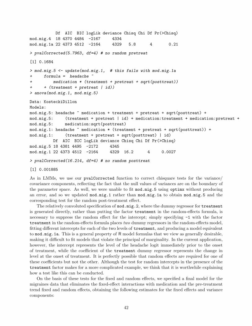
Df AIC BIC logLik deviance Chisq Chi Df Pr(>Chisq)
mod.mig.4 18 4370 4484 -2167 4334
mod.mig.1a 22 4373 4512 -2164 4329 5.8 4 0.21
> pvalCorrected(5.7963, df=4) # no random pretreat
[1] 0.1684
> mod.mig.5 <- update(mod.mig.1, # this fails with mod.mig.1a
+ formula = headache ~
+ medication * (treatment + pretreat + sqrt(posttreat))
+ + (treatment + pretreat | id))
> anova(mod.mig.1, mod.mig.5)
Data: KosteckiDillon
Models:
mod.mig.5: headache ~ medication + treatment + pretreat + sqrt(posttreat) +
mod.mig.5: (treatment + pretreat | id) + medication:treatment + medication:pretreat +
mod.mig.5: medication:sqrt(posttreat)
mod.mig.1: headache ~ medication * (treatment + pretreat + sqrt(posttreat)) +
mod.mig.1: (treatment + pretreat + sqrt(posttreat) | id)
Df AIC BIC logLik deviance Chisq Chi Df Pr(>Chisq)
mod.mig.5 18 4381 4495 -2172 4345
mod.mig.1 22 4373 4512 -2164 4329 16.2 4 0.0027
> pvalCorrected(16.214, df=4) # no random posttreat
[1] 0.001885
As in LMMs, we use our pvalCorrected function to correct chisquare tests for the variance/covariance components, reflecting the fact that the null values of variances are on the boundary ofthe parameter space. As well, we were unable to fit mod.mig.5 using optimx without producingan error, and so we updated mod.mig.1 rather than mod.mig.1a to obtain mod.mig.5 and thecorresponding test for the random post-treatment effect.
The relatively convoluted specification of mod.mig.2, where the dummy regressor for treatmentis generated directly, rather than putting the factor treatment in the random-effects formula, isnecessary to suppress the random effect for the intercept; simply specifying -1 with the factortreatment in the random-effects formula places two dummy regressors in the random-effects model,fitting different intercepts for each of the two levels of treatment, and producing a model equivalentto mod.mig.1a. This is a general property of R model formulas that we view as generally desirable,making it difficult to fit models that violate the principal of marginality. In the current application,however, the intercept represents the level of the headache logit immediately prior to the onsetof treatment, while the coefficient of the treatment dummy regressor represents the change inlevel at the onset of treatment. It is perfectly possible that random effects are required for one ofthese coefficients but not the other. Although the test for random intercepts in the presence of thetreatment factor makes for a more complicated example, we think that it is worthwhile explaininghow a test like this can be conducted.
On the basis of these tests for the fixed and random effects, we specified a final model for themigraines data that eliminates the fixed-effect interactions with medication and the pre-treatmenttrend fixed and random effects, obtaining the following estimates for the fixed effects and variancecomponents:
42

> mod.mig.6 <- glmer(headache ~ medication + treatment + sqrt(posttreat)
+ + (treatment + sqrt(posttreat) | id),
+ data=KosteckiDillon, family=binomial,
+ control=glmerControl(optimizer="optimx",
+ optCtrl=list(method="nlminb")))
> summary(mod.mig.6)
Generalized linear mixed model fit by maximum likelihood (Laplace
Approximation) [glmerMod]
Family: binomial ( logit )
Formula: headache ~ medication + treatment + sqrt(posttreat) + (treatment +
sqrt(posttreat) | id)
Data: KosteckiDillon
Control: glmerControl(optimizer = "optimx", optCtrl = list(method = "nlminb"))
AIC BIC logLik deviance df.resid
4369 4439 -2174 4347 4141
Scaled residuals:
Min 1Q Median 3Q Max
-5.182 -0.646 0.260 0.580 3.690
Random effects:
Groups Name Variance Std.Dev. Corr
id (Intercept) 1.7011 1.304
treatmentyes 1.7126 1.309 -0.12
sqrt(posttreat) 0.0571 0.239 0.11 -0.66
Number of obs: 4152, groups: id, 133
Fixed effects:
Estimate Std. Error z value Pr(>|z|)
(Intercept) -0.2459 0.3438 -0.72 0.4745
medicationreduced 2.0501 0.4679 4.38 1.2e-05
medicationcontinuing 1.1553 0.3838 3.01 0.0026
treatmentyes 1.0608 0.2439 4.35 1.4e-05
sqrt(posttreat) -0.2684 0.0449 -5.98 2.2e-09
Correlation of Fixed Effects:
(Intr) mdctnr mdctnc trtmnt
medictnrdcd -0.674
mdctncntnng -0.828 0.656
treatmentys -0.215 -0.053 -0.049
sqrt(psttr) 0.016 -0.009 -0.002 -0.685
Figure 11 shows the estimated fixed effects plotted on the probability scale; as a consequence,the post-treatment trends for the three medication conditions are not parallel, as they would be ifplotted on the logit scale:
> new.1 <- expand.grid(treatment="yes", posttreat=1:99,
43

+ medication=c("reduced", "continuing", "none"))
> new.1$treatment <- factor("yes", levels=c("no", "yes"))
> new.2 <- expand.grid(treatment="no", posttreat=-29:0,
+ medication=c("reduced", "continuing", "none"))
> new.2$posttreat <- 0
> new.2$treatment <- factor("no", levels=c("no", "yes"))
> new <- rbind(new.2, new.1)
> new$p <- predict(mod.mig.6, newdata=new, re.form=NA, type="response")
> new$time <- c(rep(-29:0, 3),rep(1:99, 3))
> plot(p ~ time, type="n", data=new, xlab="Time (days)",
+ ylab="Fitted Probability of Headache")
> abline(v=0, col="gray")
> lines(p ~ time, subset = medication == "none", data=new,
+ lty=1, lwd=2)
> lines(p ~ time, subset = medication == "reduced", data=new,
+ lty=2, lwd=2)
> lines(p ~ time, subset = medication == "continuing", data=new,
+ lty=3, lwd=2)
> legend("topright", lty=1:3, lwd=2,
+ legend=c("none", "reduced", "continuing"), title="Medication",
+ inset=.02)
It is apparent from this graph that after an initial increase at the start of treatment, the incidenceof headaches declined to substantially below its pre-treatment level. As well, the incidence ofheadaches was lowest among the patients who discontinued their medication, and highest amongthose who reduced their medication; patients who continued their medication at pre-training levelswere intermediate in headache incidence. Of course, self-selection of the medication groups rendersinterpretation of this pattern ambiguous.
4 Nonlinear Mixed Models
One extension of the nonlinear regression model (see our appendix on nonlinear regression) toinclude random effects, due to Pinheiro and Bates (2000) and fit by the nlme function in the nlmepackage,22is as follows (but with different notation than in the original source):
yi = f(θi,Xi) + εi (9)
θi = Aiβ + Biδi
where
� yi is the ni × 1 response vector for the ni observations in the ith of m groups.
� Xi is a ni × s matrix of explanatory variables (some of which may be categorical) for obser-vations in group i.
� εi ∼ Nni(0,σ2εΛi) is a ni × 1 vector of multivariately normally distributed errors for observa-
tions in group i; the matrix Λi, which is ni×ni, is typically parametrized in terms of a much
22The lme4 package also has some facilities for fitting nonlinear mixed models, but these are preliminary at thetime that we are writing this appendix.
44

−20 0 20 40 60 80 100
0.2
0.4
0.6
0.8
Time (days)
Fitt
ed P
roba
bilit
y of
Hea
dach
e
Medication
nonereducedcontinuing
Figure 11: Fixed effects from a binomial GLMM fit to the migraines data. Treatment started attime 1.
smaller number of parameters, and Λi = Ini if the observations are independently sampledwithin groups.
� θi is a ni × 1 composite coefficient vector for the observations in group i, incorporating bothfixed and random effects.
� β is the p× 1 vector of fixed-effect parameters.
� δi ∼ Nq(0,Ψ) is the q × 1 vector of random-effect coefficients for group i.
� Ai and Bi are, respectively, ni× p and ni× q matrices of known constants for combining thefixed and random effects in group i. These will often be “incidence matrices” of 0s and 1sbut may also include level-1 explanatory variables, treated as conditionally fixed (as in thestandard linear model).
Like fundamentally nonlinear fixed-effects regression models, nonlinear mixed-effects models(NLMMs) are uncommon in the social and behavioral sciences. As the following example illus-trates, however, it is occasionally natural to specify a nonlinear mixed model, especially when theparameters of the model have compelling substantive interpretations.
4.1 Example: Recovery From Coma
The data and model for this example are taken from Wong et al. (2001).23 The data pertain to200 patients who sustained traumatic brain injuries resulting in comas of varying duration. Afterawakening from their comas, patients were periodically administered a standard IQ test. In thissection, we will examine recovery of “performance IQ” (“PIQ”) post-coma; the data set, in the Wong
23We are grateful to Georges Monette for making the data and associated materials available. The analysis reportedhere is very similar to that in the original source.
45

data frame provided by the car package, also includes a measure of verbal IQ. Here are the firstfew observations in the data set:
> head(Wong)
id days duration sex age piq viq
1 3358 30 4 Male 20.67 87 89
2 3535 16 17 Male 55.29 95 77
3 3547 40 1 Male 55.92 95 116
4 3592 13 10 Male 61.66 59 73
5 3728 19 6 Male 30.13 67 73
6 3790 13 3 Male 57.06 76 69
About half of the patients in the study (107) completed a single IQ test, but the remainder weremeasured on two to five irregularly timed occasions, raising the possibility of tracing the trajectoryof IQ recovery post-coma. A mixed-effects model is very useful here because it allows us to pool theinformation in the small number of observations available per patient (on average 331/200 = 1.7)to estimate the typical within-subject trajectory of recovery along with variation in this trajectory.
After examining the data, Wong et al. posited the following asymptotic growth model for IQrecovery:
Yij = θ1i + θ2ie−θ3iX1ij + εij (10)
θ1i = β1 + β2√X2i + δ1i
θ2i = β3 + β4√X2i + δ2i
θ3i = β5
where the variables and parameters of the model have the following interpretations (see Figure 12):
� Yij is the PIQ of the ith patient (with patients indexed by id in the Wong data set) measuredon the jth occasion, j = 1, . . . , ni; as mentioned, ni = 1 for about half the patients.
� X1ij is the time post-coma (in days) for the ith patient at the jth occasion (the variable days
in the data set).
� X2i is the duration of the coma (in days) for the ith patient (duration in the data set).
� θ1i is the eventual, recovered level of PIQ for patient i, specified to depend linearly on thesquare-root of the length of the coma, with fixed-effect parameters β1 and β2, and a random-effect component δ1i. Were patients to recover PIQ fully, the average value of θ1i would be100, assuming that coma patients are representative of the general population in their pre-coma average level of IQ. Thus, the fixed-effect intercept β1 is interpretable as the expectedeventual level of PIQ for a patient in a coma of 0 days duration.
� θ2i is the negative of the amount of PIQ eventually regained by patient i, beginning at thepoint of recovery from coma. Like θ1i, the coefficient θ2i has a fixed-effect component depend-ing linearly on length of coma, with parameters β3 and β4, and a random-effect component,δ2i.
46

0 Time
PIQ
0
θ1i
− θ2i
− θ2i 2
(loge2) θ3i
Figure 12: The asymptotic growth model for recovery of IQ following coma, Yij = θ1i+θ2ie−θ3iX1ij +
εij , where Yij is the PIQ and X1ij is the time post-coma for subject i on occasion j. The parameterθ1i represents the eventual level of PIQ for subject i; −θ2i is the amount of PIQ recovered by subjecti; and θ3 is the rate of recovery for subject i (fixed across subjects), with (loge 2)/θ3 representingthe time to half-recovery.
� θ3i is the recovery rate for patient i, treated as a fixed effect, β5, with (loge 2)/θ3i repre-senting the time required to recover half the difference between final and (expected) initialpost-coma PIQ (the “half-recovery” time), that is, −θ2i/2. It makes substantive sense to treatthe patients’ recovery rates as potentially variable—that is as a random effect—but doingso introduces three additional parameters (a variance component and two covariance compo-nents) yet (as we will see below) leaves the likelihood essentially unchanged. The very smallnumber of observations per patient produces very little information in the data for estimatingpatient-specific recovery rates.
� εij is the error for patient i on occasion j.
There are, therefore, four variance-covariance components in this model, V (εij) = σ2ε , V (δ1i) =ψ21, V (δ2i) = ψ2
2, and C(δ1i, δ2i) = ψ12. Although the data are longitudinal, there are too fewobservations per patient to entertain a model with serially correlated errors.
Before fitting this model, we will examine the data, both to determine whether the positedmodel seems reasonable, and to provide rough guesses for the fixed-effects parameters. As innonlinear least squares,24. initial guesses of the fixed-effects parameters provide a starting pointfor the iterative process of maximizing the likelihood in the NLMM.
> subjects <- unique(with(Wong, id))
> with(Wong, sum(days > 1000))
[1] 40
24See the appendix on nonlinear regression
47

0 200 400 600 800 1000
6080
100
120
Days Post Coma
PIQ
Figure 13: Scatterplot for PIQ versus days since awakening from coma (dayspc). Obervationsbeyond 1000 days are not shown, and the observations for each patient are connected by gray lines.The heavier black line is for a non-parametric regression smooth.
> plot(piq ~ days, xlab="Days Post Coma",
+ ylab="PIQ", xlim=c(0, 1000),
+ data=Wong, subset = days <= 1000)
> for (subject in subjects){
+ with(Wong, lines(days[id==subject], piq[id==subject], col="gray"))
+ }
> with(Wong, lines(lowess(days, piq), lwd=2))
Figure 13 is a scatterplot of PIQ versus number of days post-coma, with the observations foreach patient connected by lines. Forty of the 331 measurements were taken after 1000 days post-coma, and these are omitted from the graph to allow us to discern more clearly the general patternof the data. The line on the plot is drawn by lowess. Mixing together the observations fromall patients makes the scatterplot difficult to interpret, but, on the other hand, there are too fewobservations for each patient to establish clear individual trajectories. Nevertheless, the asymptoticgrowth model is roughly consistent with the general pattern of the data, and the patients for whomthere are multiple observations do tend to improve over time.
> # selecting first row for each subject:
> Ag.iq <- aggregate(Wong, by=list(id=Wong$id), function(x) x[1])
> summary(Ag.iq)
id id days duration sex
Min. : 405 Min. : 405 Min. : 13 Min. : 0 Female: 43
1st Qu.:3710 1st Qu.:3710 1st Qu.: 42 1st Qu.: 1 Male :157
Median :5148 Median :5148 Median : 71 Median : 7
Mean :4778 Mean :4778 Mean : 375 Mean : 14
48

3rd Qu.:5897 3rd Qu.:5897 3rd Qu.: 172 3rd Qu.: 14
Max. :7548 Max. :7548 Max. :11628 Max. :255
age piq viq
Min. : 6.51 Min. : 50.0 Min. : 64.0
1st Qu.:21.76 1st Qu.: 74.0 1st Qu.: 83.0
Median :27.25 Median : 84.0 Median : 91.0
Mean :32.35 Mean : 83.3 Mean : 92.1
3rd Qu.:40.98 3rd Qu.: 93.0 3rd Qu.:101.2
Max. :80.03 Max. :127.0 Max. :131.0
> plot(piq ~ sqrt(duration), data=Ag.iq,
+ xlab="Days in Coma (square-root scale)", ylab="Initial PIQ",
+ axes=FALSE, frame=TRUE, subset = duration <= 100)
> (mod <- lm(piq ~ sqrt(duration), data=Ag.iq, subset = duration <= 100))
Call:
lm(formula = piq ~ sqrt(duration), data = Ag.iq, subset = duration <=
100)
Coefficients:
(Intercept) sqrt(duration)
88.49 -1.93
> abline(mod, lwd=2, lty=2)
> with(subset(Ag.iq, duration <= 100),
+ lines(lowess(sqrt(duration), piq), lwd=2))
> axis(2)
> axis(1, at=sqrt(c(0, 5, 10, seq(20, 100, by=20))),
+ labels=c(0, 5, 10, seq(20, 100, by=20)))
Figure 14 is a scatterplot of the initial PIQ measurement for each patient against the length ofthe patient’s coma (in days, on the square-root scale). These initial measurements were taken atvarying times post-coma and therefore should not be interpreted as the PIQ at time of awakening(i.e., time 0) for each patient. The relationship of initial PIQ to square-root length of coma appearsto be reasonably linear.
Figures 13 and 14 also provide a basis for obtaining initial values of the fixed-effects parametersin the mixed model of Equations 10:
� Figure 13 leads us to expect that the average eventual level of recovered IQ will be less than100, but Figure 14 suggests that the average eventual level for those who spent fewer days in
a coma should be somewhat higher; we therefore use the start value β(0)1 = 100.
� The slope of the least-squares line in Figure 14, relating initial PIQ to the square-root of
length of coma, is −1.9, and thus we take β(0)2 = −2.
� The parameter β3 represents the negative of the expected eventual gain in PIQ for a patientwho spent 0 days in a coma. On the basis of Figure 13, we will guess that such patients starton average at a PIQ of 90 and eventually recover to an average of 100, suggesting the start
value β(0)3 = −10.
49

Days in Coma (square−root scale)
Initi
al P
IQ
6080
100
120
0 5 10 20 40 60 80 100
Figure 14: Scatterplot of the initial PIQ measurement for each patient (not necessarily taken at day0) versus the number of days the patient spent in a coma (on the square-root scale). The brokenline is a least-squares line, while the solid line is a nonparametric-regression smooth.
� The parameter β4 represents the change in expected eventual PIQ gain with a 1-unit increasein the length of the coma on the square-root scale. Our examination of the data does not
provide a basis for guessing the value of this parameter, and so we will take β(0)4 = 0.
� Recall that the time to half-recovery is (loge 2)/β5. From Figure 13, it seems reasonable to
guess that the half-recovery time is around 100 days. Thus, β(0)5 = (loge 2)/100 = 0.007.
With these start values for the fixed effects, maximum-likelihood estimation of the model con-verges rapidly (but REML estimates, not shown, do not converge without simplifying the randomeffects25):
> wong.mod.1 <- nlme(piq ~ theta1 + theta2*exp(-theta3*days), data=Wong,
+ fixed=list(
+ theta1 ~ 1 + sqrt(duration),
+ theta2 ~ 1 + sqrt(duration),
+ theta3 ~ 1),
+ random=list(id = list(theta1 ~ 1, theta2 ~ 1)),
+ start=list(fixed=c(100, -2, -10, 0, 0.007)))
> summary(wong.mod.1)
Nonlinear mixed-effects model fit by maximum likelihood
Model: piq ~ theta1 + theta2 * exp(-theta3 * days)
Data: Wong
AIC BIC logLik
25We invite the reader to experiment with estimation of the model by REML, adding the argument method="REML"to the calls to nlme.
50
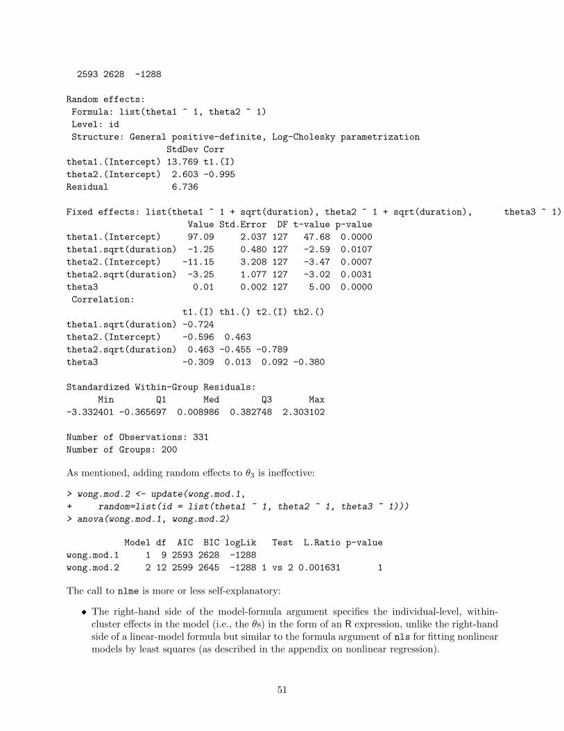
2593 2628 -1288
Random effects:
Formula: list(theta1 ~ 1, theta2 ~ 1)
Level: id
Structure: General positive-definite, Log-Cholesky parametrization
StdDev Corr
theta1.(Intercept) 13.769 t1.(I)
theta2.(Intercept) 2.603 -0.995
Residual 6.736
Fixed effects: list(theta1 ~ 1 + sqrt(duration), theta2 ~ 1 + sqrt(duration), theta3 ~ 1)
Value Std.Error DF t-value p-value
theta1.(Intercept) 97.09 2.037 127 47.68 0.0000
theta1.sqrt(duration) -1.25 0.480 127 -2.59 0.0107
theta2.(Intercept) -11.15 3.208 127 -3.47 0.0007
theta2.sqrt(duration) -3.25 1.077 127 -3.02 0.0031
theta3 0.01 0.002 127 5.00 0.0000
Correlation:
t1.(I) th1.() t2.(I) th2.()
theta1.sqrt(duration) -0.724
theta2.(Intercept) -0.596 0.463
theta2.sqrt(duration) 0.463 -0.455 -0.789
theta3 -0.309 0.013 0.092 -0.380
Standardized Within-Group Residuals:
Min Q1 Med Q3 Max
-3.332401 -0.365697 0.008986 0.382748 2.303102
Number of Observations: 331
Number of Groups: 200
As mentioned, adding random effects to θ3 is ineffective:
> wong.mod.2 <- update(wong.mod.1,
+ random=list(id = list(theta1 ~ 1, theta2 ~ 1, theta3 ~ 1)))
> anova(wong.mod.1, wong.mod.2)
Model df AIC BIC logLik Test L.Ratio p-value
wong.mod.1 1 9 2593 2628 -1288
wong.mod.2 2 12 2599 2645 -1288 1 vs 2 0.001631 1
The call to nlme is more or less self-explanatory:
� The right-hand side of the model-formula argument specifies the individual-level, within-cluster effects in the model (i.e., the θs) in the form of an R expression, unlike the right-handside of a linear-model formula but similar to the formula argument of nls for fitting nonlinearmodels by least squares (as described in the appendix on nonlinear regression).
51

� Each of the elements in the list associated with the fixed argument expresses the dependenceof the individual-level effects on the fixed effects, in the form of a linear-model formula. Theimplied coefficients on the right-hand side of these formulas are the fundamental fixed-effectparameters (i.e., the βs).
� Each of the elements of the list associated with the random argument is a linear-model formulaspecifying the random effects associated with each of the θs.
� Start values for the fixed-effect parameters (the βs), required by the nlme function, are givensequentially in the fixed element of the start argument. It is also possible to specify startvalues for the variance and covariance components, but we’ve not done that.
The nlme function accomodates much more complex specifications consistent with the NLMM ofEquations 9, but its use is reasonably straightforward in our application.
All of the estimated fixed-effects parameters are considerably larger than their standard errors.The estimated correlation between the random effects δ1i and δ2i is very high, however, rδ1δ2 =−.995. We might either simplify the model, say by eliminating random effects δ2i from the equationfor θ2i, or by reparametrizing the model to reduce the correlation between the random effects.
The estimates of the fixed effects suggest that the average final level of recovered PIQ forindividuals in a coma of 0 days duration is β̂1 = 97.1. This level declines, as anticipated, withthe length of the coma, β̂2 = −1.25. On average, patients who spend 0 days in a coma recover−β̂3 = 11.1 PIQ points, and the average size of the recovery increases with the length of the coma,−β̂4 = 3.25. The estimated half-recovery time is (loge 2)/β̂5 = (loge 2)/0.00825 = 84 days.
We can construct a fixed-effect display (Figure 15), showing how typical PIQ recovery varies asa function of days post coma and length of coma:
> newdata <- expand.grid(duration=c(1, 10, 20, 50, 100, 200),
+ days=seq(0, 1000, 20))
> newdata$piq <- predict(wong.mod.1, newdata, level=0)
> plot(piq ~ days, type="n", xlab="Days Post Coma", ylab="Average PIQ",
+ ylim=c(20, 100), xlim=c(-100, 1000), data=newdata, axes=FALSE, frame=TRUE)
> axis(2)
> axis(4)
> axis(1, at=seq(0, 1000, by=100))
> for (dc in c(1, 10, 20, 50, 100, 200)){
+ with(newdata, {
+ lines(spline(seq(0, 1000, 20), piq[duration == dc]), lwd=2)
+ text(-25, piq[duration == dc][1], labels=dc, adj=0.9)
+ })
+ }
> text(-100, 95, labels="Length\nof Coma", adj=0)
5 Complementary Reading
Much of the material in this appendix is adapted from Fox (2016, Chaps. 23 and 24). A very brieftreatment of mixed models may be found in Weisberg (2014, Sec. 7.4). Snijders and Bosker (2012)and Raudenbush and Bryk (2002) are two accessible books that emphasize hierarchical linear and,to a lesser extent, generalized-linear models. Gelman and Hill (2007) develop mixed models in the
52

Days Post Coma
Ave
rage
PIQ
2040
6080
100
2040
6080
100
0 200 400 600 800 1000
1
1020
50
100
200
Lengthof Coma
Figure 15: Fixed-effect plot of average PIQ by days since recovery from coma and length of comain days, based on the NLMM fit to the coma-recovery data.
more general context of regression analysis; these authors also discuss Bayesian approaches to mixedmodels. Stroup (2013) presents a more formal and comprehensive development of generalized linearmixed models, treating other regression models, such as linear models, generalized linear models,and linear mixed-effects models as special cases (and emphasizing SAS software for fitting thesemodels).
References
Bates, D., Maechler, M., Bolker, B., and Walker, S. (2014). lme4: Linear mixed-effects modelsusing Eigen and S4. R package version 1.1-7.
Davis, C., Blackmore, E., Katzman, D. K., and Fox, J. (2005). Female adolescents with anorexianervosa and their parents: A case-control study of exercise attitudes and behaviours. Psycholog-ical Medicine, 35:377–386.
Fox, J. (2016). Applied Regression Analysis and Generalized Linear Models. Sage, Thousand OaksCA, third edition.
Fox, J. and Weisberg, S. (2011). An R Companion to Applied Regression. Sage, Thousand Oaks,CA, second edition.
Gelman, A. and Hill, J. (2007). Data Analysis Using Regression and Multilevel/Hierarchical Models.Cambridge University Press, Cambridge UK.
Kenward, M. G. and Roger, J. (1997). Small sample inference for fixed effects from restrictedmaximum likelihood. Biometrics, 53:983–997.
53

Laird, N. M. and Ware, J. H. (1982). Random-effects models for longitudinal data. Biometrics,38:963–974.
Pinheiro, J., Bates, D., DebRoy, S., Sarkar, D., and R Core Team (2014). nlme: Linear andNonlinear Mixed Effects Models. R package version 3.1-117.
Pinheiro, J. C. and Bates, D. M. (2000). Mixed-Effects Models in S and S-PLUS. Springer, NewYork.
Raudenbush, S. W. and Bryk, A. S. (2002). Hierarchical linear models: Applications and DataAnalysis Methods. Sage, Thousand Oaks CA, second edition.
Satterthwaite, F. E. (1946). An approximate distribution of estimates of variance components.Biometrics Bulletin, 2:110–114.
Singer, J. D. (1998). Using SAS PROC MIXED to fit multilevel models, hierarchical models, andindividual growth models. Journal of Educational and Behavioral Statistics, 24:323–355.
Snijders, T. A. B. and Bosker, R. J. (2012). Multilevel Analysis: An Introduction to Basic andAdvanced Multilevel Modeling. Sage, Thousand Oaks CA, 2nd edition.
Stroup, W. W. (2013). Generalized Linear Mixed Models: Modern Concepts, Methods and Appli-cations. CRC Press, Boca Raton FL.
Weisberg, S. (2014). Applied Linear Regression. Wiley, Hoboken NJ, fourth edition.
Wong, P. P., Monette, G., and Weiner, N. I. (2001). Mathematical models of cognitive recovery.Brain Injury, 15:519–530.
54