Mitochondrial DNA analysis of genetic variation in … 2004/792...Mitochondrial DNA analysis of genetic variation in the Pacific Rim populations of chum salmon 1Yoon Moongeun, 2Vladimir

Mitochondrial DNA analysis of genetic variation in the Pacific Rim populations of chum salmon

１Yoon Moongeun, 2Vladimir Brykov, 3Nataly Varnavskaya, 4Lisa W. Seeb, 5Shigehiko Urawa, and 1Syuiti Abe

1Division of Marine Biosciences, Graduate School of Fisheries Sciences,

Hokkaido University, 3-1-1 Minato, Hakodate 041-8611, Japan 2Institute of Marine Biology, Vladivostok, Russia

3Kamchatka Research Institute of Fisheries and Oceanography, 683600, Petropavlovski-Kamchatsky, Naberejnaya 18, Russia

4Alaska Department of Fish and Game, 333 Raspberry Road, Anchorage, AK 99518, USA

5Genetics Section, National Salmon Resources Center, 2-2 Nakanoshima, Toyohira-ku, Sapporo 062-0922, Japan

Submitted to the

NORTH PACIFIC ANADROMOUS FISH COMMISSION

by

JAPAN

October 2004 �

�

�

�

�

�

�

NPAFC Doc. 792 Rev.

This paper may be cited in the following manner: Moongeun, Y., V. Brykov, N. Varnavskaya, L. W. Seeb, S. Urawa, and S. Abe. 2004. Mitochondrial DNA analysis of genetic variation in the Pacific Rim populations of chum salmon. (NPAFC Doc. 792) 25 p. Graduate School of Fisheries Sciences, Hokkaido University, 3-1-1 Minato, Hakodate 041-8611, Japan.

��

Mitochondrial DNA analysis of genetic variation in the Pacific Rim populations of chum salmon

１Yoon Moongeun, 2Vladimir Brykov, 3Nataly Varnavskaya, 4Lisa W. Seeb, 5Shigehiko Urawa, and 1Syuiti Abe

1Division of Marine Biosciences, Graduate School of Fisheries Sciences,

Hokkaido University, 3-1-1 Minato, Hakodate 041-8611, Japan 2Institute of Marine Biology, Vladivostok, Russia

3Kamchatka Research Institute of Fisheries and Oceanography, 683600, Petropavlovski-Kamchatsky, Naberejnaya 18, Russia

4Alaska Department of Fish and Game, 333 Raspberry Road, Anchorage, AK 99518, USA

5Genetics Section, National Salmon Resources Center, 2-2 Nakanoshima, Toyohira-ku, Sapporo 062-0922, Japan

ABSTRACT �

Using mitochondrial (mt) DNA analysis, we examined the genetic variation of chum salmon (Oncorhynchus keta) in 76 Pacific Rim populations including previously analyzed 48 populations and newly collected 28 populations from Russia (20 from Kamchatka, Sakhalin, Magadan, and Maritime Provinces) and North America (8 from northwest Alaska, southcentral Alaska, and Alaska Peninsula). The mtDNA haplotypes of three clades (A, B and C) observed in these additional populations were the same as those identified previously, which were defined using the DNA microarray method developed for detection of nucleotide sequence variations in the previously identified 20 variable nucleotide sites in about 500 bp portion of the 5’ end of the mtDNA control region. The occurrence of haplotypes was in keeping with our previous observations, in that clade A and C haplotypes characterized Russian populations and clade B haplotypes distinguished Alaskan populations. Thus, the observed genetic features of 76 populations examined after the analysis of molecular variance, contingency χ2 tests and pairwise population FST estimation further advocated our previous findings, which include the highest genetic variation in the Japanese populations, strong structuring among Japanese, Russia and North American populations, and a definite geographic structuring among local populations within groups. These results suggest that addition of nearly 30 populations to those examined previously provides better resolution in estimation of the genetic differentiation between or within geographic groups, and hence that incorporation of more populations in our analysis is necessary for refinement of mtDNA baseline for stock identification of mixed populations of high seas chum salmon.

INTRODUCTION �

Chum salmon (Oncorhynchus keta) have the widest natural geographical distribution among Pacific salmon species in the Pacific Rim, ranging from Korea and Japan northward to the Arctic coasts of Russia and North America and then southward to Oregon (Salo 1991). Maturing adults, like other Pacific salmons, return to the natal river.for spawning. Such restricted homing behavior will lead regional populations to partial genetic isolation.

��

Estimation of genetic variation among and within the Pacific Rim populations of chum salmon is therefore important for addressing the population history, the patterns of ocean migration, and the stock composition in high seas aggregations and coastal commercial fisheries.

Recently developed molecular techniques are likely to provide a powerful means to observe genetic variation in salmon populations with increased accuracy and resolution compared with the conventional allozyme analysis (Ferguson et al. 1995). Maternally inherited mitochondrial (mt) DNA has higher sequence variability than most single copy nuclear genes (Brown et al. 1979). The non-coding control region has been recommended for assessing intraspecific genetic variation in the species of interest, due to its higher variability than the coding regions (Moritz et al. 1987, Meyer 1993), although this situation is not always the case for some fish species (Bernatchez et al. 1992, Brown et al. 1993, Pigeon et al. 1998) including salmon (Churikov et al. 2001).

Previous analysis of restricted fragment length polymorphisms (RFLPs) showed low levels of sequence variation in limited mtDNA segments of salmonids including chum salmon (Wilson et al. 1987, Cronin et al. 1993, Park et al. 1993, Bickham et al. 1995), providing similar estimates in stock identification of mixed fisheries of chum salmon (Seeb & Crane 1999b).

Recently, Sato et al. (2001) detected greater amount of variation in the mtDNA control region by nucleotide sequence analysis than the variation observed by a previous RFLP analysis (Park et al. 1993). This finding indicates an increased potential of mtDNA sequence analysis to estimate the genetic variation of chum salmon populations.

In this study, nucleotide sequence analysis of the mtDNA control region was conducted with a newly developed DNA microarray hybridization method (Moriya et al., in press) for nearly 30 additional populations from Russia and North America. The DNA microarray immobilized synthesized oligonucleotides containing the reported sequence variations in the control region (Sato et al. 2004) on a slide glass for detection of single nucleotide polymorphisms (SNPs) (Moriya et al., in press). The obtained data, together with those obtained previously from 48 chum salmon populations (Sato et al. 2004), were analyzed to examine the potential use of mtDNA sequence variation for the analysis of the genetic variation and population structure of chum salmon in the Pacific Rim,.

MATERIALS AND METHODS �

Sampling profile. Liver, fins, or muscle samples of chum salmon were collected from 1,144 individuals

of 28 populations from Russia (20 populations) and North America (8 populations of northwest and southcentral Alaska and Alaska Peninsula) (Table 1 and Figure 1). A possible genetic difference between early- and late-run populations from five Russian population were analyzed in this study (Andyr, Kamchatk, Kalininka, Avakumovka and Megadan Rivers), as in the previous study (Sato et al. 2004). Liver samples were stored at –80°C, and fins and muscle samples were kept in ethanol at room temperature until DNA extraction.

DNA extraction.

DNA was isolated with conventional phenol-chloroform method (Sambrook et al. 1989) from the stored specimens as in our previous studies (Sato et al. 2001, 2004). Prior to extraction of DNA, the muscle samples were washed twice in 500 µl sodium tris EDTA buffer (STE; 0.1 M NaCl, 10mM Tris-HCl, and 1 mM EDTA, pH 8.0). The frozen liver samples were immediately homogenized in the same solution. About 50µl of whole blood and

��

homogenates of liver or muscle were added to 500 µl STE buffer containing 500 µg/ml proteinase K and 0.5% SDS, and incubated at 37°C overnight. DNA was extracted three times with a mixture of phenol (250 µl) and 24:1 chloroform:isoamylalcohol (250 µl), and then twice with 500 µl of the chloroform-isoamylalcohol alone. DNA in aqueous phase was recovered by ethanol precipitation, dried in air, and dissolved in tris EDTA buffer (TE; 10 mM Tris-HCl, 1 mM EDTA, pH 7.5)

DNA microarray analysis.

DNA microarray analysis of approximately 500 bp in the variable position of the 5’ end of the mtDNA control region followed the protocol developed by Moriya et al. (in press) with an OligoArray ® (Chum salmon) Kit (Nisshinbo Industries, Tokyo), according to the manufacturer’s instruction. The target region was separately amplified as two fragments using two primer pairs of 5’-AAC TAC TCT CTG GCG GCT-3’ (forward) and 5’-TTG GTG GGT AAA GAC GGA-3’ (reverse); 5’-AGT CCT GCT TAA TGT AGT-3’ (forward) and 5’-ATA AGA TTG ACA CCA TTA-3’ (reverse). Amplification was carried out in a 25 �l of reaction mixture containing 25-100 ng of template DNA, 10 mM Tris-HCl (pH 8.3), 50 mM KCl, 2.5 mM MgCl2, 0.25 mM each dNTP, 1 U Taq DNA polymerase (Shigma-Aldrich Corporation, St.Louis, MO), 1 µM of forward and reverse primers. The condition of PCR amplification using a GeneAmp PCR System 2400 (Applied Biosystems, Foster City, CA) was as follows; preheating at 95°C for 3 min, followed by 40 cycles of denaturation at 95°C for 1 min, annealing at 45°C for 30 sec, and elongation at 72°C for 30 sec, and post-cycling extensions at 72°C at 3 min. The PCR products were examined of the fragment size with 1.5% agarose-gel electrophoresis and ethidium bromide staining.

Hybridization of PCR products and signal detection followed the protocol of Moriya et al. (in press), using reagents and buffers supplied in the above kit. Two µl each of reaction mixture was denatured at 95°C for 2 min, followed by quenching on ice until hybridization. The denatured PCR product was mixed with 16 µl of hybridization buffer, mounted on a DNA microarray with cover film, and hybridized at 37°C for two hours in a moisture chamber. After hybridization, the DNA microarray was washed in a washing buffer at 37°C for 5 min. Then, 1.4 ml of conjugate solution, prepared according to the manufacturer’s instruction, was mounted on the DNA microarray and incubated at room temperature for 30 min. The DNA microarray was washed twice a coloring buffer at room temperature for 5 min each, followed by incubation with 1.4 ml of coloring solution at room temperature for 30 min. Coloring reaction was stopped by rinsing of the DNA microarray in distilled water. Air-dried DNA microarray was scanned by a GT-8700F scanner (Seiko Epson Corp., Tokyo) for visual analysis of the signal intensity on a computer. Haplotypes were determined according to the combination of signal positive-oligomer sites, which correspond to the previously identified SNPs in the target region (Sato et al. 2004).

Population genetic data analysis.

Haplotype and nucleotide diversity within populations, and nucleotide divergence between populations were estimated according to Nei (1987) and Nei and Tajima (1981) using the the Arlequin version 2.000 program package (Schneider et al., 2000). The heterogeneity of the haplotype frequencies within and between geographic regions was evaluated using the contingency χ2 test (Roff & Bentzen 1989), with 10,000 Monte Carlo simulations by CHIRXC program (Zaykin & Pudovkin 1993). Populations were grouped by the neighbor-joining (NJ) method (Saitou & Nei 1987) using pairwise nucleotide divergences. The topology obtained was tested for its stability by a consensus analysis using 1,000 replicates of the original population divergence matrix obtained by bootstrap resampling of individuals from each population. A NJ tree was constructed for each replicate with NEIGHBOR and

��

the consensus tree was generated using CONSENSUS in PHYLIP version 3.5c software (Felsenstein 1993). In order to assess the extent of genetic divergence at different levels of geographic hierarchy, the overall molecular variance was partitioned into components corresponding to the population divergence within and among regions by the analysis of molecular variance model (AMOVA; Excoffier et al. 1992) using the above Arlequin program package. Pairwise FST values were calculated to estimate the genetic distance between populations according to (Slatkin 1995), using the Arlequin program. Significance of the variance components and FST values was tested with a permutation method.

RESULTS �

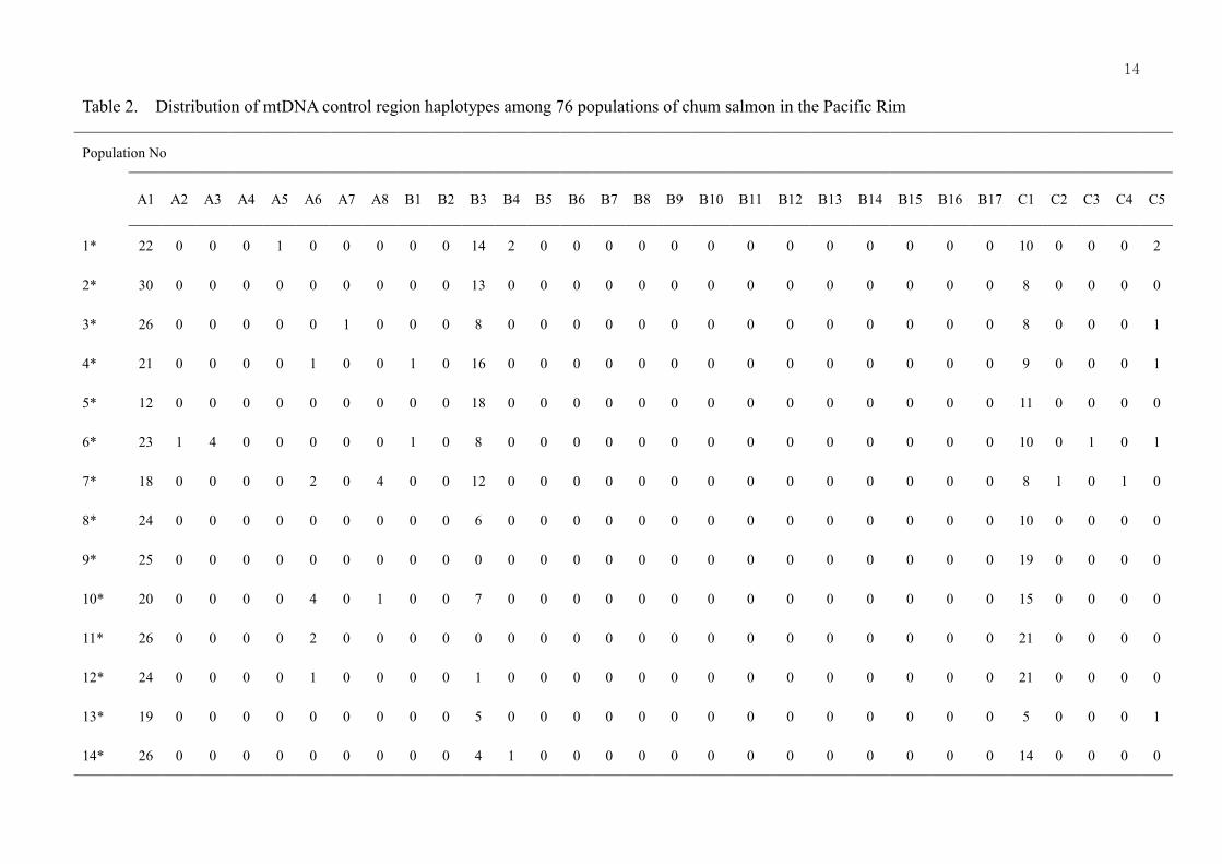
Distribution of mtDNA control region haplotypes in chum salmon. The mtDNA haplotypes of three clades (A, B and C) observed in 28 additional

populations were the same as those identified previously (Sato et al. 2004). Distribution of 30 haplotypes among 76 populations of chum salmon, including those examined herein and analyzed previously (Sato et al., 2004), is presented in Table 2. The observed haplotypes in the present 28 populations from Russia and North America was mostly the same as those found in our previous observations (Sato et al. 2004) and further advocated an association with geographic regions, in that clade A nd C haplotypes characterized Asia and Russian populations and clade C haplotypes distinguish Alaskan population.

Fifteen haplotypes occurred in a total of 30 Russian populations. All the three haplotype clades occurred in the populations from Primorye region on the Sea of Japan coast (39, 40 and 41) and Belaya population (34) from Sakhalin in Russia, as in the populations from Japan and Korea (see Table 2 and Fig. 1). Twenty eight populations in other Russian regions contained clade B and C haplotypes except for the Taranay (36) and Okhotskoe population (38), which showed only the clade B haplotypes (Table 2). The clade C haplotypes were less abundant than clade B haplotypes, and the haplotype B-3 was predominant in most of the Russian populations (Table 2).

The number of haplotypes in North American populations was apparently less than that of the populations in Japan and Russia even in the eight additional populations. The North American populations exhibited no clade A haplotypes, and clade C haplotypes were rare (<2%) and occurred in only three populations, one from the Alaska Peninsula (Belkofski, 61) and the others from Kodiak Island (Kizhuyak River, 57) and McNeil River (60) (see Table 2 and Fig. 1).

The occurrence of the B-13 haplotype was common in North American populations except for two populations in southcentral Alaska, Kitoi Hatchery (59) and McNeil River (60) and all nine populations in northwestern Alaska, Salmon River (48), Yukon River and its tributary (Sheenjak River, 49; Andreafsky River, 50; Tanana River, 53), Togiak River (51), Noatak (52), Unalakleet (54), Kwethluk River (55) and Upper Nushagak (56). These northwestern populations were fixed or nearly fixed for the B-3 haplotype (Table 2 and Fig. 1). Other North American populations usually included one or two clade B haplotypes, in addition to the B-3 and B-13 haplotypes.

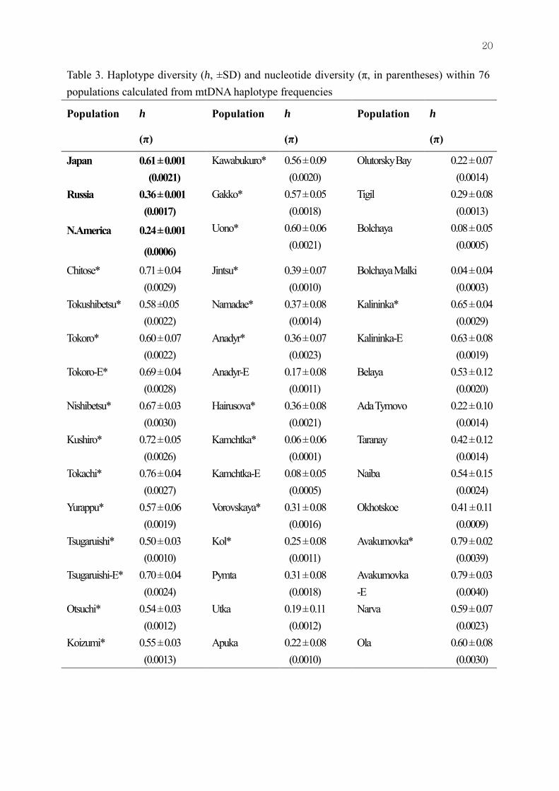
Genetic variability in the Pacific Rim populations.

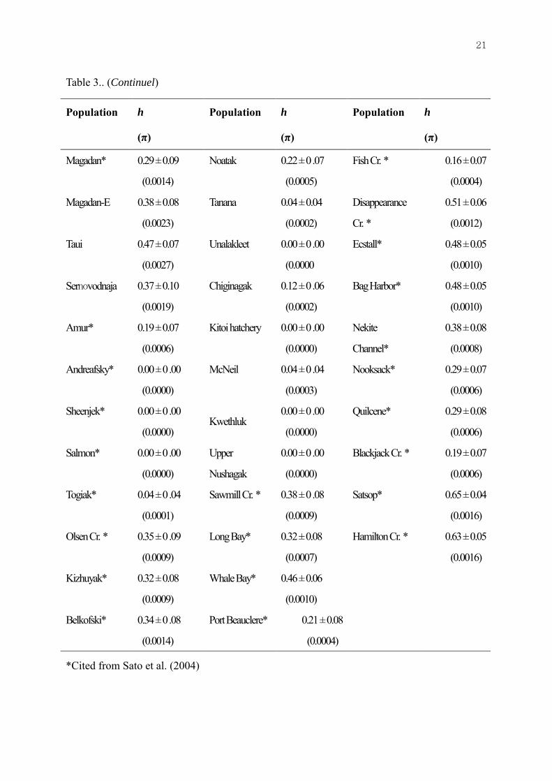
Haplotype diversity was highest in the populations of Japan (0.63±0.001), followed by those of Russia (0.36±0.001) and North America (0.24±0.001), whereas nucleotide diversity was similar in the Japanese (0.0021) and Russian populations (0.0017), but lower in the North American populations (Table 3). These findings suggest greater genetic variation in the populations of Japan than those of Russia and North America.

��

Heterogeneity in the haplotype distribution.

The contingency χ2 test showed highly significant heterogeneity (p<0.001) in the haplotype frequencies for the entire set of populations (Table 4). Significant regional heterogeneity (p<0.001) was also observed between each set of populations from Japan and Russia, Japan and North America, and Russia and North America, respectively, in addition to within each region except for British Columbia (Table 4). In Russia, no heterogeneity in the haplotype distribution was found between early- and late-run fish from Anadyr, Kamchatka and Avakumovka Rivers, but a distinct heterogeneity was shown in those from Kalininka and Magadan Rivers (p<0.001).

Geographic differentiation in the Pacific Rim populations.

A consensus NJ tree of 76 populations separated the Japanese (plus Korean), Russian and North American populations with subclusters of local populations within each geographical group (not shown), as in our previous study (Sato et al., 2004). Using population groups suggested by the NJ method, AMOVAs (Table 5) revealed the following population structure in the Pacific Rim chum salmon populations; very strong geographic structuring among Japan, Russia, and North America (56.8% of the total variance, p<0.001, Analysis I), as compared with the average extent of structuring among populations within each geographic group (6.2% of the total variance); similar level of population structuring among three regional groups in Japan (7.6% of the variance, p<0.001, Analysis II), among five regional groups in North America (7.0% of the variance, p<0.001, Analysis IV), and among six regional groups of Russia (25.35% of the variance, p<0.001, Analysis III). These results suggest a definite geographic structuring among local populations within groups, which was not apparent, particularly, in Russia in our previous study (Sato et al. 2004).

As shown in Table 6, pairwise FST estimates were greater between Japan and North America (0.520 to 0.947) than between Japan and Russia (-0.007 to 0.929) or between Russia and North America (-0.014 to 0.817). These results further advocated the distinct structuring among Japanese, Russia and North American populations inferred from the AMOVAs as above.

DISCUSSION �

The present study recruited 28 chum salmon populations from Russia and Alaska for mtDNA sequence analysis using the newly developed DNA microarray hybridization technique. All the haplotypes observed in these additional populations were not new and have been described in our previous study (Sato et al. 2004). The distribution of haplotypes in these populations also was in keeping with the previous observation (Sato et al. 2004), i.e. predominance of the clade B and C haplotypes in Russia and fixation to the clade B haplotypes, with few clade C haplotypes, in North America. These findings suggest that not many additional haplotypes may be expected even when recruited more populations from Russia and North America.

Rapid and accurate identification of haplotypes was provided by the present DNA microarray, with which detection of haplotypes in more than 1,100 individuals was completed within two months. This method requires only standard laboratory equipments such as a thermal cycler for PCR, incubator for hybridization, waterbath for post-hybridization washing, and office scanner for computer assist of signal intensity analysis. In addition, all the experimental process is finished less than 8 hours, except for DNA extraction. This technical simplicity of DNA microarray to detect all the reported SNPs for haplotype

��

identification of chum salmon mtDNA will be applicable to less equipped hatchery or works on board ship. In fact, mtDNA haplotypes of about 1,000 chum salmon have been determined during a research cruise sponsored by the Fisheries Agency, Japan, in the Bering Sea September 2002 (Moriya et al. 2004).

The AMOVA, contingency χ2 test and pairwise FST estimates revealed clear geographic structuring in the Pacific Rim chum salmon populations, with distinct genetic divergence among Japan, Russia, and North America. Previously, we could not estimate geographic hierarchy in the genetic structure of Russian populations due to the insufficient number of available populations (Sato et al. 2004). In the present study, addition of 20 populations from Kamchatka, Sakhalin, Magadan, and southern Primorye to the previously examined 10 populations has made it possible to disclose the genetic differentiation among local groups in Russia with a substantial statistical support by AMOVA (25.35%, p<0.001, Table 5). As well, incorporation of 8 Alaskan populations provided an increased resolution in the geographic differentiation among local groups in North America (7.0% variance, p<0.001, Table 5), compared with the previous estimation (4.9% variance, p<0.005) by Sato et al. (2004).

Genetic divergence among the three regional groups of chum salmon was also observed in the previous studies using variation of allozyme loci (Okazaki 1983, Wilmot et al. 1998, Seeb & Crane 1999a), mtDNA RFLPs (Seeb & Crane 1999b), and minisatellite DNA (Taylor et al. 1994). Furthermore, several allozyme studies have also inferred geographic structuring within regions (Kondzela et al. 1994, Phelps et al. 1994, Wilmot et al. 1994, Wilmot et al. 1998, Seeb & Crane 1999a). Nevertheless, an increased extent of genetic divergence among and within geographical groups revealed by the present mtDNA analysis seems to provide better resolution in the divergence estimation than that expected from the previous allozyme and DNA analyses.

Thus, the present findings apparently indicate an improvement of divergence estimation among the Pacific Rim populations of chum salmon after incorporation of nearly 30 additional populations in our mtDNA analysis. Current mtDNA data may therefore become useful for constructing a baseline for stock identification of mixed populations of high seas chum salmon, if more populations are recruited in analysis.

ACKNOWLEDGMENTS

This study was supported in part by Grants-in-Aid from the Fisheries Agency, Japan, and from the North Pacific Research Board to the NPAFC Cooperative Research (R0303).

REFERENCES �

Bernatchez, L., R. Guyomard & F. Bonhomme. 1992. DNA sequence variation of the mitochondrial control region among geographically and morphologically remote European brown trout Salmo trutta populations. Mol. Ecol. 1: 161-173.

Bickham, J. W., C. C. Wood & J. C. Patton. 1995. Biogeographic implications of cytochrome b sequences and allozymes in sockeye (Oncorhynchus nerka). J. Hered. 86: 140-144.

Brown, W. M., M. George, Jr. & A. C. Wilson. 1979. Rapid evolution of animal mitochondrial DNA. Proc. Natl. Acad. Sci. U. S. A 76: 1967-1971.

Churikov, D., M. Matsuoka, X. Luan, A.K. Gray, V.A. Brykov & A.J. Gharrett. 2001. Assessment of concordance among genealogical reconstructions from various mtDNA segments in three species of Pacific salmon (genus Oncorhynchus). Mol. Ecol. 10:

��

2329-2339. Cronin, M. A., W. J. Spearman, R. L. Wilmot, J. C. Patton & J. W. Bickham. 1993.

Mitochondrial DNA variation in chinook (Oncorhynchus tshawytscha) and chum salmon (O. keta) detected by restriction enzyme analysis of polymerase chain reaction (PCR) products. Can. J. Fish. Aquat. Sci. 50: 708-715.

Excoffier, L., P. E. Smouse & J. M. Quattro. 1992. Analysis of molecular variance inferred from metric distances among DNA haplotypes: application to human mitochondrial DNA restriction data. Genetics 131: 479-491.

Felsenstein, J. 1993. PHYLIP (Phylogeny inference package), Version 3.5c. Department of Genetics, University of Washington, Seattle: available at the web site http://evolution.genetics.washington.edu/phylip.html.

Ferguson, A., J. B. Taggart, P. A. Prodohl, O. Mcmeel, C. Thompson, C. Stone, P. Mcginnity & R. A. Hynes. 1995. The application of molecular markers to the study and conservation of fish populations, with special reference to salmo. J. Fish. Biol. 47 (Suppl. A) : 103-126.

Kondzela, C. M., C. M. Guthrie, S. L. Hawkins, C. D. Russell, J. H. Helle & A. J. Gharrett. 1994. Genetic relationship among chum salmon populations in southeast Alaska and northern British Columbia. Can. J. Fish. Aquat. Sci. 51: 50-64.

Meyer, A. 1993. Evolution of mitochondrial DNA in fish. pp. 1-38. In: P. W. Hochachka &� � T. P. Mommsen (ed.) Biochemistry and Molecular Biology of Fishes, Volume 2, Elsevier, Amstrdam.

Moritz, C., T. E. Dowling & W. M. Brown. 1987. Evolution of animal mitochondrial DNA: relevance for population biology and systematics. Ann. Rec. Ecol. Syst. 18: 269-292.

Moriya, S., S. Urawa, O. Suzuki, A. Urano& S. Abe. 2003. DNA microarray for rapid detection of mitochondrial DNA haplotypes of chum salmon. Mar. Biotechnol., in press

Okazaki, T. 1983. Genetic structure of chum salmon Oncorhynchus keta river populations. Bull. Jap. Soc. Sci. Fish. 49: 189-196.

Park, L. K., M. A. Brainard, D. A. Dightman & G. A. Winans. 1993. Low levels of intraspecific variation in the mitochondrial DNA of chum salmon (Oncorhynchus keta). Mol. Mar. Biol. Biotech. 2: 362-370.

Phelps, S. R., L. L. Leclair, S. Young & H. L. Iankenship. 1994. Genetic diversity patterns of chum salmon in the Pacific northwest. Can. J. Fish. Aquat. Sci. 51 (Suppl. 1): 65-83.

Pigeon, D., J. J. Dodson & L. Bernatchez. 1998. A mtDNA analysis of spatiotemporal distribution of two sympatric larval populations of rainbow smelt (Osmerus mordax) in the St. Lawrence River estuary, Quebec, Canada. Can. J. Fish. Aquat. Sci. 55: 1739-1747.

Roff, D. A. & P. Bentzen. 1989. The statistical analysis of mitochondrial DNA polymorphisms: chi 2 and the problem of small samples. Mol. Biol. Evol. 6:539-545.

Saitou, N. & M. Nei. 1987. The neighbor-joining method: a new method for reconstructing phylogenetic trees. Mol. Biol. Evol. 4: 406-425.

Salo, E. O. 1991. Life history of chum salmon (Oncorhynchus keta). pp. 231-309. In C. Groot & L. Margolis (ed.) Pacific Salmon Life Histories. University of British Columbia Press, Vancouver.

Sambrook, J., E. F. Fritsch & T. Maniatis. 1989. Molecular Cloning: A Laboratory Manual, 2 ed. Cold Spring Harbor Laboratory Press, New York.

Sato, S., J. Ando, H. Ando, S. Urawa, A. Urano & S. Abe. 2001. Genetic variation among Japanese populations of chum salmon inferred from the nucleotide sequences of the mitochondrial DNA control region. Zool. Sci. 18: 99-106.

http://evolution.genetics.washington.edu/phylip.html

�

Sato, S., H. Kojima, J. Ando, H. Ando, R. L. Wilmot, L. W. Seeb, V. Efremov, L. LeClair, W. Buchholz, D. H. Jin, S. Urawa, M. Kaeriyama, A. Urano & S. Abe. 2004. Genetic population structure of chum salmon in the Pacific Rim inferred from mitochondrial DNA sequence variation. Environ. Biol. Fish. 69: 37-50.

Schneider, S., D. Roessli & L. Excoffier. 2000. Arlequin. Version 2.000 University of Geneva, Geneva: available at the web site http://lgb.unige.ch/arlequin/.

Seeb, L. W. & P. A. Crane. 1999a. High genetic heterogeneity in chum salmon in western Alaska, the contact zone between northern and southern lineages. Trans. Am. Fish. Soc. 128: 58-87.

Seeb, L. W. & P. A. Crane. 1999b. Allozymes and mitochondrial DNA discriminate Asian and north American populations of chum salmon in mixed-stock fisheries along the south coast of the Alaska Peninsula. Trans. Am. Fish. Soc. 128: 88-103.

Taylor, E. B., T. D. Beacham & M. Kaeriyama. 1994. Population structure and identification of north Pacific Ocean chum salmon (Oncorhynchus keta) revealed by an analysis of minisatellite DNA variation. Can. J. Fish. Aquat. Sci. 51: 1430-1442.

Wilmot, R. L., R. J. Everett, W. J. Spearman, R. Baccus, N. V. Varnavskaya & S. V. Putivkin. 1994. Genetic stock structure of western Alaska chum salmon and a comparison with Russia far east stocks. Can. J. Fish. Aquat. Sci. 51 (Suppl. 1): 84-94.

Wilmot, R. L., C. M. Kondzela, C. M. Guthrie & M. M. Masuda. 1998. Genetic stock identification of chum salmon harvested incidentally in the 1994 and 1995 Bering Sea trawl fishery. N. Pac. Anadr. Fish. Comm. Bull. 1: 285-299.

Wilson, G. M., W. K. Thomas & A. T. Beckenbach. 1987. Mitochondrial DNA analysis of Pacific northwest populations of Oncorhynchus tshawytscha. Can. J. Fish. Aquat. Sci. 44: 1301-1305.

Zaykin, D. V. & A. I. Pudovkin. 1993. Two programs to estimate significance of χ2 values using pseudo-probability tests. J. Hered. 84: 152.

http://lgb.unige.ch/arlequin/

�

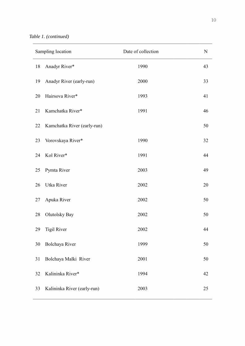
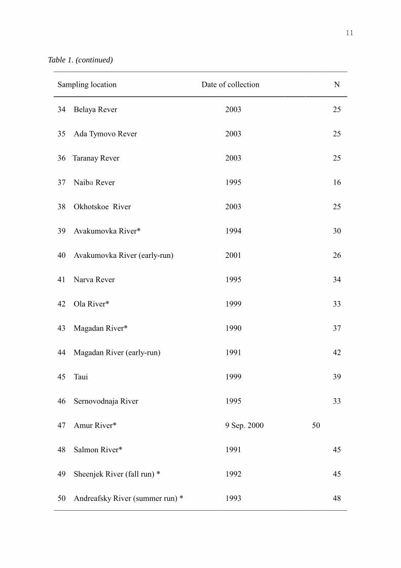
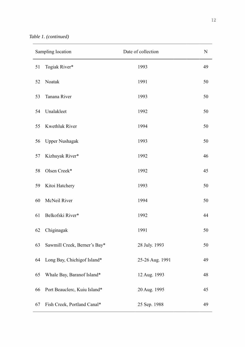
Table 1. Sampling locations, date of collection, and the numbers of chum salmon samples (N) used for mtDNA analysis

Sampling location Date of collection N

1 Chitose River* 14 Oct. 1996 51

2 Tokushibetsu River* 23 Sep. 1997 51

3 Tokoro River (late run)* 20 Nov. 1998 44

4 Tokoro River (early run)* 13 Oct. 1999 49

5 Nishibetsu River* 25 Sep. 1997 41

6 Kushiro River* 22 Oct. 1998 49

7 Tokachi River* 17 Oct. 1996 46

8 Yurappu River* 17 Nov. 1998 40

9 Tsugaruishi River (late run), Iwate Pref.* 10 Dec. 1997 44

10 Tsugaruishi River (early run), Iwate Pref.* Oct. 1999 47

11 Otsuchi River, Iwate Pref.* 8 Apr. 1999 49

12 Koizumi River, Miyagi Pref.* 21 Nov. 1996 47

13 Kawabukuro River, Akita Pref. * 18 Nov. 1997 30

14 Gakko River, Yamagata Pref.* 10 Dec. 1996 45

15 Uono River, Nigata Pref.* 23-24 Oct. 1996 49

16 Jintsu River, Toyama Pref.* 7 Nov. 1995 49

17 Namadae River 13 Nov. 2000 46

��

Table 1. (continued)


18 Anadyr River* 1990 43

19 Anadyr River (early-run) 2000 33

20 Hairsova River* 1993 41

21 Kamchatka River* 1991 46

22 Kamchatka River (early-run) 50

23 Vorovskaya River* 1990 32

24 Kol River* 1991 44

25 Pymta River 2003 49

26 Utka River 2002 20

27 Apuka River 2002 50

28 Olutolsky Bay 2002 50

29 Tigil River 2002 44

30 Bolchaya River 1999 50

31 Bolchaya Malki River 2001 50

32 Kalininka River* 1994 42

33 Kalininka River (early-run) 2003 25

��



34 Belaya Rever 2003 25

35 Ada Tymovo Rever 2003 25

36� �Taranay Rever 2003 25

37 Naiba Rever 1995 16

38 Okhotskoe River 2003 25

39 Avakumovka River* 1994 30

40 Avakumovka River (early-run) 2001 26

41 Narva Rever 1995 34

42 Ola River* 1999 33

43 Magadan River* 1990 37

44 Magadan River (early-run) 1991 42

45 Taui 1999 39

46 Sernovodnaja River 1995 33

47 Amur River* 9 Sep. 2000 50

48 Salmon River* 1991 45

49 Sheenjek River (fall run) * 1992 45

50 Andreafsky River (summer run) * 1993 48

��



51 Togiak River* 1993 49

52 Noatak 1991 50

53 Tanana River 1993 50

54 Unalakleet 1992 50

55 Kwethluk River 1994 50

56 Upper Nushagak 1993 50

57 Kizhuyak River* 1992 46

58 Olsen Creek* 1992 45

59 Kitoi Hatchery 1993 50

60 McNeil River 1994 50

61 Belkofski River* 1992 44

62 Chiginagak 1991 50

63 Sawmill Creek, Berner’s Bay* 28 July. 1993 50

64 Long Bay, Chichigof Island* 25-26 Aug. 1991 49

65 Whale Bay, Baranof Island* 12 Aug. 1993 48

66 Port Beauclerc, Kuiu Island* 20 Aug. 1995 45

67 Fish Creek, Portland Canal* 25 Sep. 1988 49

��



68 Disappearance Creek, POW Island* 25 Sep. 1998 50

69 Ecstall River, Skeena River area* 12 Sep. 1988 45

70 Bag Harbor, QCI* mid-Oct. 1989 50

71 Nekite Channel* 15 Sep. 1989 33

72 Nooksack River* 1998 47

73 Quilcene Bay* 1998 49

74 Blackjack Creek* 1998 50

75 Satsop River* 1998 49

76 Hamilton Creek* 1998 43

*Cited from Sato et al. (2004)

��

Table 2. Distribution of mtDNA control region haplotypes among 76 populations of chum salmon in the Pacific Rim

Population No

A1 A2 A3 A4 A5 A6 A7 A8 B1 B2 B3 B4 B5 B6 B7 B8 B9 B10 B11 B12 B13 B14 B15 B16 B17 C1 C2 C3 C4 C5

1* 22 0 0 0 1 0 0 0 0 0 14 2 0 0 0 0 0 0 0 0 0 0 0 0 0 10 0 0 0 2

2* 30 0 0 0 0 0 0 0 0 0 13 0 0 0 0 0 0 0 0 0 0 0 0 0 0 8 0 0 0 0

3* 26 0 0 0 0 0 1 0 0 0 8 0 0 0 0 0 0 0 0 0 0 0 0 0 0 8 0 0 0 1

4* 21 0 0 0 0 1 0 0 1 0 16 0 0 0 0 0 0 0 0 0 0 0 0 0 0 9 0 0 0 1

5* 12 0 0 0 0 0 0 0 0 0 18 0 0 0 0 0 0 0 0 0 0 0 0 0 0 11 0 0 0 0

6* 23 1 4 0 0 0 0 0 1 0 8 0 0 0 0 0 0 0 0 0 0 0 0 0 0 10 0 1 0 1

7* 18 0 0 0 0 2 0 4 0 0 12 0 0 0 0 0 0 0 0 0 0 0 0 0 0 8 1 0 1 0

8* 24 0 0 0 0 0 0 0 0 0 6 0 0 0 0 0 0 0 0 0 0 0 0 0 0 10 0 0 0 0

9* 25 0 0 0 0 0 0 0 0 0 0 0 0 0 0 0 0 0 0 0 0 0 0 0 0 19 0 0 0 0

10* 20 0 0 0 0 4 0 1 0 0 7 0 0 0 0 0 0 0 0 0 0 0 0 0 0 15 0 0 0 0

11* 26 0 0 0 0 2 0 0 0 0 0 0 0 0 0 0 0 0 0 0 0 0 0 0 0 21 0 0 0 0

12* 24 0 0 0 0 1 0 0 0 0 1 0 0 0 0 0 0 0 0 0 0 0 0 0 0 21 0 0 0 0

13* 19 0 0 0 0 0 0 0 0 0 5 0 0 0 0 0 0 0 0 0 0 0 0 0 0 5 0 0 0 1

14* 26 0 0 0 0 0 0 0 0 0 4 1 0 0 0 0 0 0 0 0 0 0 0 0 0 14 0 0 0 0

��

�



15* 29 0 0 2 0 0 0 0 0 0 8 0 0 0 0 0 0 0 0 0 0 0 0 0 0 9 0 0 0 1

16* 37 0 0 0 0 0 0 0 0 0 2 0 0 0 0 0 0 0 0 0 0 0 0 0 0 10 0 0 0 0

17* 36 0 0 0 0 0 0 0 0 0 6 0 0 0 0 0 0 0 0 0 0 0 0 0 0 3 0 0 0 1

18* 0 0 0 0 0 0 0 0 0 0 35 0 0 0 0 0 0 0 0 0 0 0 0 0 0 9 0 0 0 1

19 0 0 0 0 0 0 0 0 0 0 30 0 0 0 0 0 0 0 0 0 0 0 0 0 0 3 0 0 0 0

20* 0 0 0 0 0 0 0 0 0 0 32 0 0 0 0 0 1 0 0 0 0 0 0 0 0 8 0 0 0 0

21* 0 0 0 0 0 0 0 0 0 0 31 0 0 0 1 0 0 0 0 0 0 0 0 0 0 0 0 0 0 0

22 0 0 0 0 0 0 0 0 0 0 48 0 0 0 0 0 0 0 0 0 0 0 0 0 0 2 0 0 0 0

23* 0 0 0 0 0 0 0 0 0 0 38 0 0 0 0 0 1 0 0 1 0 0 0 0 0 6 0 0 0 0

24* 0 0 0 0 0 0 0 0 0 0 38 0 0 0 0 0 2 0 0 1 0 0 0 0 0 3 0 0 0 0

25 0 0 0 0 0 0 0 0 0 0 40 0 0 0 0 0 1 0 0 0 0 0 0 0 0 8 0 0 0 0

26 0 0 0 0 0 0 0 0 0 0 18 0 0 0 0 0 0 0 0 0 0 0 0 0 0 2 0 0 0 0

27 0 0 0 0 0 0 0 0 0 0 44 0 0 0 0 0 0 0 0 0 0 3 0 0 0 3 0 0 0 0

28 0 0 0 0 0 0 0 0 0 0 44 0 0 0 0 0 0 0 0 0 0 0 0 0 0 6 0 0 0 0

��



29 0 0 0 0 0 0 0 0 0 0 37 0 0 0 0 0 3 0 0 0 0 0 0 0 0 4 0 0 0 0

30 0 0 0 0 0 0 0 0 0 0 48 0 0 0 0 0 0 0 0 0 0 0 0 0 0 2 0 0 0 0

31 0 0 0 0 0 0 0 0 0 0 49 0 0 0 0 0 0 0 0 0 0 0 0 0 0 1 0 0 0

32* 0 0 0 0 0 0 0 0 0 0 20 0 0 0 0 0 16 0 0 0 0 0 0 0 0 7 0 0 1 0

33 0 0 0 0 0 0 0 0 0 0 14 0 0 0 0 6 4 0 0 0 0 0 0 0 0 1 0 0 0 0

34 1 0 0 0 0 0 0 0 0 0 17 0 0 0 0 2 3 0 0 0 0 0 0 0 0 2 0 0 0 0

35 0 0 0 0 0 0 0 0 0 0 22 0 0 0 0 0 0 0 0 0 0 0 0 0 0 3 0 0 0 0

36 0 0 0 0 0 0 0 0 1 0 19 0 0 0 0 1 3 0 0 0 0 0 0 0 0 0 0 0 0 0

37 0 0 0 0 0 0 0 0 1 0 11 0 0 0 0 1 1 0 0 0 0 0 0 0 0 1 0 0 1 0

38 0 0 0 0 0 0 0 0 0 0 19 0 0 0 0 4 2 0 0 0 0 0 0 0 0 0 0 0 0 0

39* 7 0 0 0 0 0 0 0 0 0 9 0 0 0 0 1 0 0 0 0 0 0 0 0 0 6 0 0 0 7

40 4 0 0 0 0 0 0 0 0 0 7 0 0 0 0 1 0 0 0 0 0 0 0 0 0 7 0 0 0 7

41 8 0 0 0 0 0 0 0 0 0 6 0 0 0 0 0 0 0 0 0 0 0 0 0 0 20 0 0 0 0

42* 0 0 0 0 0 0 0 0 1 0 20 0 0 1 0 0 3 0 0 0 0 0 0 0 0 7 0 0 0 1

43* 0 0 0 0 0 0 0 0 0 4 31 0 0 0 0 0 1 0 0 0 0 0 0 0 0 0 1 0 0 0

��



44 0 0 0 0 0 0 0 0 0 0 32 0 0 0 0 0 1 0 0 0 0 0 0 0 0 9 0 0 0 0

45 0 0 0 0 0 0 0 0 1 0 27 0 0 0 0 0 0 0 0 0 0 0 0 0 0 10 0 0 0 1

46 3 0 0 0 0 1 0 0 0 0 26 0 0 0 0 0 0 0 0 0 0 0 0 0 0 3 0 0 0 0

47* 0 0 0 0 0 0 0 0 2 0 45 0 0 0 0 0 2 0 0 0 0 0 0 0 0 1 0 0 0 0

48* 0 0 0 0 0 0 0 0 0 0 48 0 0 0 0 0 0 0 0 0 0 0 0 0 0 0 0 0 0 0

49* 0 0 0 0 0 0 0 0 0 0 45 0 0 0 0 0 0 0 0 0 0 0 0 0 0 0 0 0 0 0

50* 0 0 0 0 0 0 0 0 0 0 45 0 0 0 0 0 0 0 0 0 0 0 0 0 0 0 0 0 0 0

51* 0 0 0 0 0 0 0 0 0 0 48 0 0 0 0 0 0 0 0 0 0 0 1 0 0 0 0 0 0 0

52 0 0 0 0 0 0 0 0 0 0 44 0 0 0 0 0 5 0 0 1 0 0 0 0 0 0 0 0 0 0

53 0 0 0 0 0 0 0 0 0 1 49 0 0 0 0 0 0 0 0 0 0 0 0 0 0 0 0 0 0 0

54 0 0 0 0 0 0 0 0 0 0 50 0 0 0 0 0 0 0 0 0 0 0 0 0 0 0 0 0 0 0

55 0 0 0 0 0 0 0 0 0 0 50 0 0 0 0 0 0 0 0 0 0 0 0 0 0 0 0 0 0 0

56 0 0 0 0 0 0 0 0 0 0 49 0 0 0 0 0 0 0 0 0 0 0 0 0 0 0 0 0 0 0

57* 0 0 0 0 0 0 0 0 0 0 36 0 0 0 0 0 1 0 0 0 6 0 0 0 0 1 0 0 0 0

�

��



58* 0 0 0 0 0 0 0 0 0 0 35 0 0 0 0 0 0 0 2 0 6 0 0 0 2 0 0 0 0 0

59 0 0 0 0 0 0 0 0 0 0 49 0 0 0 0 0 0 0 0 0 0 0 0 0 0 0 0 0 0 0

60 0 0 0 0 0 0 0 0 0 0 49 0 0 0 0 0 0 0 0 0 0 0 0 0 0 1 0 0 0 0

61* 0 0 0 0 0 0 0 0 0 0 37 0 0 0 0 0 0 0 0 0 5 0 0 0 0 4 0 0 0 0

62 0 0 0 0 0 0 0 0 0 0 47 0 0 0 0 0 0 0 0 0 3 0 0 0 0 0 0 0 0 0

63* 0 0 0 0 0 0 0 0 0 0 39 0 0 0 0 0 1 0 5 0 5 0 0 0 0 0 0 0 0 0

64* 0 0 0 0 0 0 0 0 0 0 40 0 0 0 0 0 1 0 1 0 7 0 0 0 0 0 0 0 0 0

65* 0 0 0 0 0 0 0 0 0 0 33 0 0 0 0 0 2 0 0 0 13 0 0 0 0 0 0 0 0 0

66* 0 0 0 0 0 0 0 0 0 0 40 0 0 0 0 0 4 0 0 0 1 0 0 0 0 0 0 0 0 0

67* 0 0 0 0 0 0 0 0 0 0 45 0 0 0 0 0 0 0 0 0 3 0 0 0 1 0 0 0 0 0

68* 0 0 0 0 0 0 0 0 0 0 33 0 0 0 0 0 5 0 0 0 12 0 0 0 0 0 0 0 0 0

69* 0 0 0 0 0 0 0 0 0 0 29 0 0 0 0 0 1 0 0 0 15 0 0 0 0 0 0 0 0 0

70* 0 0 0 0 0 0 0 0 0 0 32 0 0 0 0 0 0 0 1 0 17 0 0 0 0 0 0 0 0 0

�

�

��



71* 0 0 0 0 0 0 0 0 0 0 39 0 0 0 0 0 0 0 0 0 8 0 0 0 0 0 0 0 0 0

72* 0 0 0 0 0 0 0 0 0 0 41 0 0 0 0 0 0 3 0 0 5 0 0 0 0 0 0 0 0 0

73* 0 0 0 0 0 0 0 0 0 0 45 0 0 0 0 0 0 0 0 0 3 0 0 2 0 0 0 0 0 0

74* 0 0 0 0 0 0 0 0 0 0 45 0 0 0 0 0 0 0 0 0 3 0 0 2 0 0 0 0 0 0

75* 0 0 0 0 0 0 0 0 0 0 23 0 0 0 0 0 1 0 0 0 17 8 0 0 0 0 0 0 0 0

76* 0 0 0 0 0 0 0 0 0 0 23 0 6 0 0 0 0 0 0 0 12 2 0 0 0 0 0 0 0 0

Total 441 1 4 2 1 11 1 5 8 5 2154 3 6 1 1 16 65 3 9 3 145 13 1 2 3 332 2 1 2 26


�

�

�

�

�

�

�

��

Table 3. Haplotype diversity (h, ±SD) and nucleotide diversity (π, in parentheses) within 76 populations calculated from mtDNA haplotype frequencies

Population h

(π)

Population h

(π)

Population h

(π)

Japan 0.61 ± 0.001 (0.0021)

Kawabukuro* 0.56 ± 0.09 (0.0020)

Olutorsky Bay 0.22 ± 0.07 (0.0014)

Russia 0.36 ± 0.001 (0.0017)

Gakko* 0.57 ± 0.05 (0.0018)

Tigil 0.29 ± 0.08 (0.0013)

N.America 0.24 ± 0.001

(0.0006)

Uono* 0.60 ± 0.06 (0.0021)

Bolchaya 0.08 ± 0.05 (0.0005)

Chitose* 0.71 ± 0.04 (0.0029)

Jintsu* 0.39 ± 0.07 (0.0010)

Bolchaya Malki 0.04 ± 0.04 (0.0003)

Tokushibetsu* 0.58 ±0.05 (0.0022)

Namadae* 0.37 ± 0.08 (0.0014)

Kalininka* 0.65 ± 0.04 (0.0029)

Tokoro* 0.60 ± 0.07 (0.0022)

Anadyr* 0.36 ± 0.07 (0.0023)

Kalininka-E 0.63 ± 0.08 (0.0019)

Tokoro-E* 0.69 ± 0.04 (0.0028)

Anadyr-E 0.17 ± 0.08 (0.0011)

Belaya 0.53 ± 0.12 (0.0020)

Nishibetsu* 0.67 ± 0.03 (0.0030)

Hairusova* 0.36 ± 0.08 (0.0021)

Ada Tymovo 0.22 ± 0.10 (0.0014)

Kushiro* 0.72 ± 0.05 (0.0026)

Kamchtka* 0.06 ± 0.06 (0.0001)

Taranay 0.42 ± 0.12 (0.0014)

Tokachi* 0.76 ± 0.04 (0.0027)

Kamchtka-E 0.08 ± 0.05 (0.0005)

Naiba 0.54 ± 0.15 (0.0024)

Yurappu* 0.57 ± 0.06 (0.0019)

Vorovskaya* 0.31 ± 0.08 (0.0016)

Okhotskoe 0.41 ± 0.11 (0.0009)

Tsugaruishi* 0.50 ± 0.03 (0.0010)

Kol* 0.25 ± 0.08 (0.0011)

Avakumovka* 0.79 ± 0.02 (0.0039)

Tsugaruishi-E* 0.70 ± 0.04 (0.0024)

Pymta 0.31 ± 0.08 (0.0018)

Avakumovka -E

0.79 ± 0.03 (0.0040)

Otsuchi* 0.54 ± 0.03 (0.0012)

Utka 0.19 ± 0.11 (0.0012)

Narva 0.59 ± 0.07 (0.0023)

Koizumi* 0.55 ± 0.03 (0.0013)

Apuka 0.22 ± 0.08 (0.0010)

Ola 0.60 ± 0.08 (0.0030)

��

Table 3.. (Continuel)

Population h

(π)

Population h

(π)

Population h

(π)

Magadan* 0.29 ± 0.09

(0.0014)

Noatak 0.22 ± 0 .07

(0.0005)

Fish Cr. * 0.16 ± 0.07

(0.0004)

Magadan-E 0.38 ± 0.08

(0.0023)

Tanana 0.04 ± 0.04

(0.0002)

Disappearance

Cr. *

0.51 ± 0.06

(0.0012)

Taui 0.47 ± 0.07

(0.0027)

Unalakleet 0.00 ± 0 .00

(0.0000

Ecstall* 0.48 ± 0.05

(0.0010)

Sernovodnaja 0.37 ± 0.10

(0.0019)

Chiginagak 0.12 ± 0 .06

(0.0002)

Bag Harbor* 0.48 ± 0.05

(0.0010)

Amur* 0.19 ± 0.07

(0.0006)

Kitoi hatchery 0.00 ± 0 .00

(0.0000)

Nekite

Channel*

0.38 ± 0.08

(0.0008)

Andreafsky* 0.00 ± 0 .00

(0.0000)

McNeil 0.04 ± 0 .04

(0.0003)

Nooksack* 0.29 ± 0.07

(0.0006)

Sheenjek* 0.00 ± 0 .00

(0.0000) Kwethluk

0.00 ± 0 .00

(0.0000)

Quilcene* 0.29 ± 0.08

(0.0006)

Salmon* 0.00 ± 0 .00

(0.0000)

Upper

Nushagak

0.00 ± 0 .00

(0.0000)

Blackjack Cr. * 0.19 ± 0.07

(0.0006)

Togiak* 0.04 ± 0 .04

(0.0001)

Sawmill Cr. * 0.38 ± 0 .08

(0.0009)

Satsop* 0.65 ± 0.04

(0.0016)

Olsen Cr. * 0.35 ± 0 .09

(0.0009)

Long Bay* 0.32 ± 0.08

(0.0007)

Hamilton Cr. * 0.63 ± 0.05

(0.0016)

Kizhuyak* 0.32 ± 0.08

(0.0009)

Whale Bay* 0.46 ± 0.06

(0.0010)

Belkofski* 0.34 ± 0 .08

(0.0014)

Port Beauclere* 0.21 ± 0.08

(0.0004)


��

Table 4. The probability of homogeneity for pairwise geographic regions was given below diagonal, which was calculated using contingency χ2 test with 10,000 Monte Carlo simulations (Roff & Bentzen 1989). The probability of homogeneity within regions was given on diagonal.

Japan Russia North America

Region HOK HON KAM SAK PRI MAG SER AMU NWA AP/ SCLA

SEA BCL WSG

Hokkaido (8) <0.001

Honshu (8) <0.001 <0.001

Kamchtka (14) <0.001 <0.001 0.002

Sakhalin (7) <0.001 <0.001 <0.001 <0.001

Primory (3) <0.001 <0.001 <0.001 <0.001 0.010

Magadan (4) <0.001 <0.001 <0.001 <0.001 <0.001 0.002

Sernovodnaja (1) <0.001 <0.001 <0.001 <0.001 <0.001 <0.001 �

Amur (1) <0.001 <0.001 <0.001 <0.001 <0.001 <0.001 0.017 �

Northwest Alaska (9)

<0.001 <0.001 <0.001 <0.001 <0.001 <0.001 <0.001 <0.001 <0.001

Alaska Peninsula/ Southcentral Alaska(6)

<0.001 <0.001 <0.001 <0.001 <0.001 <0.001 <0.001 <0.001 <0.001 0.002

Southeast Alaska (6) <0.001 <0.001 <0.001 <0.001 <0.001 <0.001 <0.001 <0.001 <0.001 <0.001 <0.001

British Columbia (3) <0.001 <0.001 <0.001 <0.001 <0.001 <0.001 <0.001 <0.002 <0.001 <0.001 <0.001 0.755

Washington (5) <0.001 <0.001 <0.001 <0.001 <0.001 <0.001 <0.001 <0.001 <0.001 <0.001 <0.001 <0.001 <0.001

��

Table 5. Results of the hierarchical analyses of molecular variance for chum salmon. The percentage of variance (%), probability estimated from permutation (P), and the F-statistics (Ф) are given at hierarchical level (Excoffier et al. 1992).

Variance component % P �Ф

Analysis I

Among three regional groups

(Japan, Russia, and North America)

56.83 <0.001 0.68

Among populations within groups 6.2 <0.001 0.075

Within populations 37.0 <0.001 0.44

Analysis II

Among three regional groups in Japan

(Hokkaido, Japan sea coast, Pacific ocean coast)

7.6 <0.001 0.064



Analysis III

Among six regional groups in Russia

(Kamchtka, Sakhallin, Primorye, Megadan, Sernovodnaja ,

Amur)

25.35 <0.001 0.20



Analysis IV

Among five regional groups in North America

(Northwest Alaska, Alaska Peninsula/Southcentral Alaska,

Southeast Alaska, British Columbia, Washington)

7.06 <0.001 0.012



�

��

Table 6. Pairwise FST.estimates for regional chum salmon populations excluding one Korean population by mtDNA sequence analysis. Maximum (top)

and minimum (bottom) FST values within and between regions are shown

Japan Russia North America Region HOK HON KAM SAK PRI MAG SER AMU NWA AP/

SCLA SEA BCL WSG

Hokkaido (8) 0.129 -0.016

Honshu (8) 0.351 -0.028

0.132 -0.026

Kamchtka (14) 0.746 -0.004

0.929 -0.007

0.167 -0.034

Sakhalin (7) 0.737 0.228

0.898 0.500

0.198 -0.032

0.142 -0.044

Primory (3) 0.090 0.002

0.245 0.023

0.782 0.272

0.724 0.293

0.047 -0.031

Magadan (4) 0.737 0.128

0.898 0.390

0.241 -0.019

0.209 -0.008

0.723 0.189

0.124 -0.020

Sernovodnaja (1) 0.516 0.183

0.725 0.492

0.162 -0.020

0.138 0.024

0.343 0.297

0.063 -0.018

0.000 0.000

Amur (1) 0.766 0.476

0.903 0.731

0.138 -0.010

0.161 0.007

0.588 0.636

0.214 0.133

0.122 0.000

0.000 0.000

Northwest Alaska (9)

0.823 0.520

0.947 0.758

0.211 -0.002

0.239 0.057

0.817 0.643

0.294 0.056

0.214 0.190

0.016 -0.002

0.067 0.002

Alaska Peninsula/ Southcentral Alaska(6)

0.820 0.470

0.946 0.634

0.290 -0.013

0.237 -0.014

0.815 0.465

0.292 0.008

0.212 0.033

0.063 -0.009

0.076 0.000

0.100 -0.007

Southeast Alaska (6) 0.797 0.495

0.925 0.737

0.208 0.025

0.222 0.056

0.791 0.600

0.272 0.078

0.202 0.176

0.144 0.067

0.244 0.049

0.228 -0.017

0.138 -0.012

British Columbia (3) 0.770 0.471

0.904 0.721

0.248 0.101

0.252 0.123

0.763 0.571

0.291 0.125

0.231 0.179

0.212 0.134

0.306 0.237

0.311 0.001

0.219 -0.013

0.000 -0.020

Washington (5) 0.790 0.471

0.918 0.711

0.223 0.038

0.235 0.068

0.784 0.568

0.276 0.079

0.216 0.180

0.200 0.041

0.260 0.055

0.265 -0.011

0.199 -0.010

0.120 -0.010

0.132 0.000

��

Figure 1. Geographical position of sampling site (see Table 1 for the site names).

Documents

Mitochondrial DNA analysis of genetic variation in … 2004/792...Mitochondrial DNA analysis of genetic variation in the Pacific Rim populations of chum salmon 1Yoon Moongeun, 2Vladimir