Minimum Wages and Employment: A Case Study of the Fast ... Media... · journals and scholarly literature from ... A Case Study of the Fast-Food Industry in New Jersey ... wage led

Minimum Wages and Employment A Case Study of the Fast-Food Industry inNew Jersey and Pennsylvania Reply

David Card Alan B Krueger

The American Economic Review Vol 90 No 5 (Dec 2000) pp 1397-1420

Stable URL

httplinksjstororgsicisici=0002-82822820001229903A53C13973AMWAEAC3E20CO3B2-2

The American Economic Review is currently published by American Economic Association

Your use of the JSTOR archive indicates your acceptance of JSTORs Terms and Conditions of Use available athttpwwwjstororgabouttermshtml JSTORs Terms and Conditions of Use provides in part that unless you have obtainedprior permission you may not download an entire issue of a journal or multiple copies of articles and you may use content inthe JSTOR archive only for your personal non-commercial use

Please contact the publisher regarding any further use of this work Publisher contact information may be obtained athttpwwwjstororgjournalsaeahtml

Each copy of any part of a JSTOR transmission must contain the same copyright notice that appears on the screen or printedpage of such transmission

The JSTOR Archive is a trusted digital repository providing for long-term preservation and access to leading academicjournals and scholarly literature from around the world The Archive is supported by libraries scholarly societies publishersand foundations It is an initiative of JSTOR a not-for-profit organization with a mission to help the scholarly community takeadvantage of advances in technology For more information regarding JSTOR please contact supportjstororg

httpwwwjstororgMon Jul 2 135246 2007

Minimum Wages and Employment A Case Study of the Fast-Food Industry in New Jersey and Pennsylvania Reply

Replication and reanalysis are important en- deavors in economics especially when new find- inns run counter to conventional wisdom In their u

Comment on our 1994 American Economic Re- view article David Neumark and William Was- cher (2000) challenge our conclusion that the April 1992 increase in the New Jersey minimum wage led to no loss of employment in the fast-food industry Using data drawn from payroll records for a set of restaurants initially assembled by Rich- ard Berman of the Employment Policies Institute (EPI) and later supplemented by their own data- collection efforts Neumark and Wascher (hereaf- ter NW) conclude that the New Jersey minimum-wage increase led to a relative decline in fast-food employment in New Jersey com-pared to ~enns~1vanial They attribute the discrep- ancies between their findings and ours to problems in our fast-food restaurant data set Specifically they argue that our use of employment data derived from telephone surveys rather than from

Card Department of Economics Evans Hall Univer- sity of California Berkeley CA 94720 and National Bu- reau of Economic Research Krueger Department of Economics Princeton University Princeton NJ 08544 and National Bureau of Economic Research The analysis in Sections I 11and In subsection E of this paper is based on confidential Bureau of Labor Statistics (BLS) ES-202 data The authors thank the BLS staff for assistance with these data Although the BLS data are confidential persons employed by an eligible organization may apply to BLS for restricted access to ES-202 data for statistical research purposes Data from our 1994 paper are available via anony- mous FTP from the minimum directory of irsprincetonedu All opinions and analysis in this paper reflect the views of the authors and not the US government We thank seminar participants at Princeton University the National Bureau of Economic Research the University of Pennsylvania the University of California-Berkeley the Kennedy School (Harvard University) and Lany Katz and John Kennan for helpful comments and the Princeton University Industrial Relations Section for research support

In the March 1995 version of their paper NW relied exclusively on 71 observations collected by EPI Subse- quent versions have also included information from their supplemental data collection

payroll records led us to draw faulty inferences about the effect of the New Jersey minimum wane

u

In this paper we attempt to reconcile the contrasting findings by analyzing administrative employment data from a new representative sample of fast-food employers in New Jersey and Pennsylvania and by reanalyzing NWs data Most importantly we use the Bureau of Labor Statisticss (BLSs) employer-reported ES-202 data file to examine employment growth of fast-food restaurants in a set of major chains in New Jersey and nearby counties of ~ e n n s ~ l v a n i a ~We draw two samples from the ES-202 files a longitudinal file that tracks a fixed sample of establishments between 1992 and 1993 and a series of repeated cross sections from the end of 1991 through 1997 Because the BLS data are derived from unemployment-insurance (UI) payroll-tax records the employment measures are free of the kinds of survey errors that NW allege affected our earlier results In addition because the ES-202 data include information for all covered employers in a fixed group of restaurant chains there is no reason to doubt the representativeness of the BLS sample

A comparison of fast-food employment growth in New Jersey and Pennsylvania over the period of our original study confirms the key findings in our 1994 paper and calls into question the representativeness of the sample assembled by Berman Neumark and Wascher Consistent with our original sample the BLS fast-food data set indicates slightly faster employment growth in New Jersey than in the Pennsylvania border counties over the time period that we initially examined although in most specifications the differential is small and statistically insignificant We also use the BLS

The ES-202 data are also known as the Business Es- tablishment List

1395 THE AMERICAN ECONOMIC REVIEW DECEMBER 2000

data to examine longer-run effects of the New Jersey minimum-wage increase and to study the effect of the 1996 increase in the federal minimum wage which was binding in Pennsyl- vania but not in New Jersey where the state minimum wage already exceeded the new federal standard Our analysis of this new policy intervention provides further evidence that modest changes in the minimum wage have little systematic effect on employment

In light of these results ~ e - ~ o on to reexamine the Berman-Neumark-Wascher (BNW) sample and evaluate NWs contention that the rise in the New Jersey minimum wage caused employment to fall in the states fast-food industry Our reanalysis leads to four main conclusions First the pattern of employment growth in the BNW sample of fast-food restaurants across chains and geographic areas within New Jersey is remarkably consistent with our original survey data In both data sets employment grew faster in areas of New Jersey where wages were forced up more by the 1992 minimum-wage increase The differences between the BNW sample and ours are attributable to differences in the BNW sample of Pennsylvania restaurants which unlike the more comprehensive BLS sample and our original sample shows a rise in fast-food employment in the state Second the differential employment trend in the BNW Pennsylvania sample is driven by data for restaurants from a single Burger King franchisee who provided all the Pennsylvania data in the original Berman sample

Third the employment trends measured in the BNW sample are significantly different for restaurants that reported their payroll data on a weekly biweekly or monthly basis Establish- ments that reported on a biweekly basis had faster growth than those that reported on a monthly or weekly basis We suspect that the different reporting bases matter because the BNW employment measure is based on payroll hours (rather than actual numbers of employees) and because weekly biweekly and monthly averages of payroll hours were differentially affected by seasonal factors including the Thanksgiving holiday and a major winter storm in December 1992 Regardless of the explana- tion a higher fraction of Pennsylvania restaurants reported their data in biweekly intervals leading to a faster measured employment

growth in that state Once the employment changes are adjusted for the reporting bases the BNW sample shows virtually identical growth in New Jersey and eastern Pennsylvania Fi- nally a reanalysis of publicly available BLS data on employment trends in the two states shows no effect of the minimum wage on employment in the eating and drinking industry

Based on all the evidence now available including the BLS ES-202 sample our earlier sample publicly available BLS data and the BNW sample we conclude that the increase in the New Jersey minimum wage in April 1992 had little or no systematic effect on total fast- food employment in the state although there may have been individual restaurants where employment rose or fell in response to the higher minimum wage

I Analysis of Representative BLS Fast-Food Restaurant Sample

A Description of BLS ES-202 Data

On April 1 1992 the New Jersey state minimum wage increased from $425 to $505 per hour while the minimum wage in Pennsylvania remained at $425 To examine the effect of the New Jersey minimum-wage increase using representative payroll data we applied to the BLS for permission to analyze their ES-202 data The ES-202 database consists of employment records reported quarterly by employers to their state employment security agencies for unemployment-insurance tax purposes The first question on the New Jersey UI tax form requests the Number of covered workers em-ployed during the pay period which includes the 12th day of each month3 The BLS maintains these data as part of the Covered Employment

The first question on the Pennsylvania form requests the Total covered employees in pay period incl 12th of month Employers are asked to report employment for each month of the quarter A copy of these forms is available from the authors on request Other points to note about the ES-202 data include they are not restricted to employers with any minimum number of employees or to employees who have earned any minimum pay in the pay period there is no information on hours of work the pay period may vary across employers or within employers for different workers employees on vacation or sick leave should be included if they are paid while absent from work

1399 VOL 90 NO 5 CARD AND KRUEGER MINIMUM WAGE AND EMPLOYMENT REPLY

and Wages Program We analyze two types of samples from the ES-202 file a longitudinal file and a series of repeated cross sections

The longitudinal sample consists of restaurants belonging to a set of the largest fast-food chainsS4 Restaurants in the sampled chains employed 13 percent of all employees in the eating and drinking industry in New Jersey and eastern Pennsylvania in 1992 There is considerable overlap between the restaurants in the BLS sample and those in our original sample5 Our sample of fast-food restaurants from the ES-202 data was drawn as follows We first selected all records for all establishments in the eating and drinking industry (SIC 5812) in New Jersey and eastern Pennsylvania in the first quarter of 1991 first quarter of 1994 and fourth quarter of 1996 Then restaurants in the sampled chains were identified from this universe by separately searching for the chains names or variants of their names in the legal name trade name and unit description fields of the ES-202 file If the name of an included chain was mentioned in any of these text fields the record was then visually examined to ensure that it belonged in the sample of included restaurant In addition records for all eating and drinking establishments from these quarters were visually in-spected to identify any fast-food restaurants in the relevant chains that were missed by the computerized name search If a restaurant in one of the relevant fast-food chains was discov- ered that was not identified by the initial name search the computerized name-search algo-rithm was amended to include that restaurant

The original Card-Krueger (CK) sample contained data on restaurants in 7 counties of Penn- sylvania (Bucks Chester Lackawanna Lehigh Luzerne Montgomery and Northampton) Be- cause this is a somewhat idiosyncratic group- with some counties located right on the New Jersey border and others off the border-we decided to expand the sample to include 7 additional counties Berks Carbon Delaware

For confidentiality reasons BLS has requested that we not reveal the identity or number of these chains We can report however that there are fewer than 10 chains in the sample

We reached this conclusion by comparing the distribu- tion of restaurants by three-digit zip code and chain in the two data sets

Monroe Philadelphia Pike and Wayne In the results that follow we present estimates for both our original 7 counties and for the larger set of 14 counties The map in Figure 1 indicates the location of the restaurants in our initial survey the original 7 counties in Pennsylvania and the additional 7 counties in Pennsylvania

Once restaurants in the relevant chains and counties were identified we merged quarterly records for these restaurants for the period from the first quarter of 1992 to the fourth quarter of 1994 to create a longitudinal file6 To mirror the CK sample only establishments with nonzero employment in February or March of 1992- the months covered by wave 1 of our survey- were included in the longitudinal analysis file The final longitudinal sample contains 687 establishments A total of 16 (23 percent) of these establishments had zero or missing employment in November or December of 1992 the months covered by wave 2 of our original survey These establishments either closed or could not be tracked because their reporting information changed In 1992 less than 1 percent of establishments had imputed employment data (that is cases where the state filled in an estimate of employment because the establishment failed to report it)

A potential limitation of the BLS longitudinal sample for the present paper should be noted The ES-202 data pertain to reporting units that may be either single establishment units or multiestablishment units The BLS encouraged employers to report their data at the county level or below in the early 1990s Some employers were in the process of switching to a county- level reporting basis during our sample period Consequently some restaurants that remained open were difficult to track because they changed their reporting identifiers Fortunately most of the restaurants that were in this situation could be tracked by searching addresses and other characteristics of the stores All of the

Additionally to ensure that the sample consisted exclusively of restaurants (as opposed to eg headquarters or monitoring posts) the authors restricted the sample to establishments with an average of five or more employees in February and March 1994 and average monthly payroll per employee below $3000 in 1992Ql and 1992Q4 These restrictions eliminated 17 observations from the original sample of 704 observations


Original 7 Cwnties

Additional 7 Counties

Number of Restaurants in Original Survey

1

FIGURE 1 AREAS OF NEW JERSEY AND PENNSYLVANIA COVERED BY ORIGINAL SURVEY AND BLS DATA

restaurants that were not linked to subsequent months data were assumed closed and assigned zero employment for these months even though some of these restaurants may not have closed This is probably a more common occurrence for New Jersey than Pennsylvania 04 percent of the Pennsylvania restaurants had zero or missing employment at the end of 1992 as com- pared to 34 percent of New Jersey restaurants In our original survey 13 percent of Pennsyl- vania restaurants and 27 percent of New Jersey restaurants were temporarily or permanently closed at the end of 1992~

Also note that because firms are allowed to report on more than one unit in a county in the BLS data some of the records reflect an aggre- gation of data for multiple establishments We address both of these issues in the analysis below Importantly however these problems do not affect the repeated cross-sectional files that we also analyze

An interviewer visited all of the nonresponding stores in both states to determine if they were closed in our original survey

To draw the repeated cross-sectional file the final name-search algorithm described above was applied each quarter between 1991Q4 and 1997Q3 Again data were selected for the same chains in New Jersey and the 14 counties in eastern Pennsylvania Every months data from the sampled quarters was selected The cross-sectional sample probably provides the cleanest estimates of the effect of the minimum- wage increase because it incorporates births as well as deaths of restaurants and because possible problems caused by changes in reporting units over time are minimized

B Summary Statistics and Differences-in- Differences

Table 1 reports basic employment summary statistics for New Jersey and for the Pennsylva- nia counties before and after the April 1992 increase in New Jerseys minimum wage Panel A is based on the longitudinal BLS sample of fast-food restaurants In the first row the before period pertains to average employment in February and March of 1992 and the after pertains to average employment in November


TABLE 1-DESCRLPTIVE STATISTICS RESTAURANTS FROM BLS ES-202 FOR FAST-FOOD DRAWN

A BLS ES-202 Data February-March 1992 to

November-December 1992

February 1992 to November 1992

March 1992 to March 1993

B Card-Krueger Survey Data February 1992 to November 1992

DATAAND CARD-KRUEGERSURVEY

Means with standard deviations in parentheses

New Jersey 7 Pennsylvania counties 14 Pennsylvania counties

Before After Change Before After Change Before After Change

372 (199)

372 (199)

372 (201)

298 (125)

Notes Sample sizes for the first two rows are 437 for New Jersey 127 for Pennsylvania 7 counties and 250 for Pennsylvania 14 counties sample sizes for third row are 436 127 and 250 respectively sample sizes for the last row are 309 for New Jersey and 75 for Pennsylvania The 7 Pennsylvania counties used in the middle columns are the same counties used in Card and Krueger (1994) these 7 counties are a subset of the 14 counties in the last three columns (see text) The unit of observation for the BLS data is the reporting unit which in some cases includes multiple establishments The unit of observation in the Card-Kmeger data is the individual restaurant

and December of 1992 The second row re-ports employment figures for February and No- vember which were the most common survey months in our original telephone survey The third row shows data for the 12-month interval from March 1992 to March 1993 Finally for comparison panel B of Table 1 reports the corresponding employment statistics calculated from the CK survey Note that for comparability with BLS data we have calculated total em-ployment for restaurants in our original survey by adding together the number of full-time part-time and managerial worker^^

Several conclusions are apparent from the means in Table 1 First the BLS data indicate a slight rise in employment in New Jerseys fast- food restaurants over the period we studied and a slight decline in employment in Pennsylva- nias restaurants over the same period Our telephone survey data indicate a net gain in New Jersey relative to Pennsylvania of 24 workers per restaurant whereas the BLS data in row 2 indicate a smaller net gain of 11 workers be-

In one case employment was zero in March 1992 so the February figure was used

This approach differs from Card and Kmeger (1994) which weights part-time workers by 05 to derive full-time equivalent employment

tween February and November of 1992 Sec- ond between March 1992 and March 1993 the BLS data indicate that both New Jersey and Pennsylvania experienced a decline in average employment with the decline being larger in Pennsylvania Third the average employment level in the BLS data is somewhat greater than the average level in our data probably because some of the observations in the BLS data pertain to multiple establishments Fourth our data and the BLS data both suggest that average restaurant size was initially larger in Pennsyl- vania than in New Jersey By contrast the BNW data set indicates that full-time equivalent employment was initially greater in New Jersey than in Pennsylvania (see Section 111 below) Finally the BLS data indicate that the results for the 7 Pennsylvania counties that we used in our initial sample and the wider set of 14 coun-ties are generally similar

Neumark and Wascher (2000) and others have emphasized the fact that the dispersion in full-time employment changes in our data set is greater than the dispersion in changes in total hours worked in the BNW data Interestingly the BLS payroll data display roughly the same standard deviation of employment changes as was found in our original sample For example in New Jersey the standard deviation of the


change in employment across reporting units between February and November of 1992 was 1012 in the BLS data which slightly exceeds the standard deviation calculated from our survey data (982) over approximately the same months One problem with this comparison is that some of the BLS reporting units combine two or more restaurants that mav have been broken out over time whereas the unit of observation in our original survey was the individual restaurant To address this issue we restricted the BLS sample to reporting units that initially had fewer than 40 employees these smaller reporting units are almost certainly individual restaurants The standard deviation of employment changes for this truncated BLS sample is 90 for New Jersey and 68 for Penn- sylvania these figures compare to 80 and 88 respectively if we likewise truncate our survey data

More generally the criticism that our telephone survey was flawed because of the sub- stantial dispersion in measured employment growth in our sample strikes us as off the mark for three reasons First reporting errors in employment data collected from a telephone survey are not terribly surprising Dispersion in our data is not out of line with measures based on other establishment-level employment surveys (eg Steven J Davis et al 1996)1deg Second employment changes are the dependent variable in our analysis As long as the measurement error process is the same for restaurants in New Jersey and Pennsylvania estimates of the difference i n employment growth based on our data will be unbiased We know of no reason to suspect that the New Jersey and Pennsylvania managers who responded to our survey would misreport employment data in a systematically different way Moreover all of our telephone interviews were conducted by a single profes- sional interviewer Third any comparison of the standard deviation of full-time equivalent employment changes is potentially sensitive to the

Although Neumark and Wascher (2000 footnote 9) argue that variability in employment growth should be smaller for fast-food restaurants in a small geographic area than in a sample such as Davis et als set of manufacturing establishments it should be noted that gross employment flows are considerably higher in the retail trade sector than in the manufacturing sector (see Julia Lane et al 1996)

way data on hours or combinations of part-time and full-time employees are scaled For example in their analysis NW convert weekly payroll hours data into a measure of employment by dividing by 35 but a smaller divisor would obviously lead to larger dispersion of employment in their data The standard deviation of proportionate changes in employment is invari- ant to scaling and is fairly similar in all three data sets 029 in the BLS data 035 in BNWs data and 039 in our earlier survey data

C Regression-Adjusted Models

Panels A and B of Table 2 present basic regression estimates using the BLS ES-202 longitudinal sample of fast-food restaurants The models presented in this table essentially parallel the main specifications in Card and Krueger (1994) The dependent variable in the first two columns is the change in the number of employees while the dependent variable in the last two columns is the proportionate change in the number of employees Following Card and Krueger (1994) the denominator of the proportionate change is the average of first- and second-period employment Employ- ment changes are measured between February- March 1992 and November-December 1992 Columns (1) and (3) include as the only regressor a dummy variable indicating whether the restaurant is located in New Jersey or eastern Penn- sylvania These estimates correspond to the difference-in-differences estimates that can be derived from row 1 of Table 1 The models in columns (2) and (4) add a set of additional control variables dummy variables for the identity of the restaurant chain and a dummy variable indicating whether the reporting unit was a subunit of a multiunit employer

The regression results in panel A of Table

The proportionate employment change was calculated as the change in employment divided by the initial level of employment We use total number of full-time and part- time workers in our data for comparability to the BLS data Neumark and Wascher (2000) show that some other ways of measuring the proportionate change of employment (eg using average employment in the denominator) and some sample restrictions (eg eliminating closed stores from the sample) increases the dispersion in our data relative to theirs

l2Observations that are not reported as subunits of multiunit establishments are either part of a multiunit reporting


TABLE2-BASIC RESULTS DATAAND CARD-KRUEGER DATAREGRESSION BLS ES-202 FAST-FOOD SURVEY

Dependent variable

Change in levels Proportionate change

Explanatory variables (1) (2) (3) (4)

A All of New Jersey and 7 Pennsylvania Counties BLS Data

New Jersey indicator 0536 0225 0007 0009 (1017) (1029) (0029) (0029)

Chain dummies and subunit dummy variable No Yes No Yes Standard error of regression 1009 999 0286 028 1 R~ 0001 0029 0000 0046

B All of New Jersey and 14 Pennsylvania Counties BLS Data


Chain dummies and subunit dummy variable No Yes No Yes Standard error of regression 1080 1063 0303 0294 R~ 0002 0042 0005 0071

C Original Card-Krueger Survey Data

New Jersey indicator 241 1 2488 0029 0030 (1323) (1323) (0050) (0049)

Chain and company-ownership dummies No Yes No Yes Standard error of regression 1028 1025 0385 0382 R~ 0009 0025 0001 0024

Notes Each regression also includes a constant Sample size is 564 for panel A 687 for panel B and 384 for panel C Subunit dummy variable equals one if the reporting unit is a subunit of a multiunit employer For comparability with the BLS data employment in the CK sample is measured by the total number of full- and part-time employees Standard errors are in parentheses

2 which are based on the employment changes minimum wage Only in the proportionate for restaurants in the same geographic region change specifications without covariates how- surveyed in our earlier work indicate small ever is the difference in growth rates between positive coefficients on the New Jersey dummy New Jersey and ~ e n n s ~ l v a n i a restaurants close variableI3 Each of the estimates is individually to being statistically significant statistically insignificant however We interpret For comparison panel C contains the corre- these estimates as indicating that New Jerseys sponding estimates from our original sample employment growth in the fast-food industry These estimates differ (slightly) from those re- over this period was essentially the same as it ported in our original paper because we now was for the same set of restaurant chqins in the measure employment as the unweighted sum of 7 Pennsylvania counties full-time workers part-time workers and man-

In panel B regression results are presented agerial workers to-be comparable to the BLS using the wider set of 14 Pennsylvania counties data The estimates based on our sample are as the comparison group These results also qualitatively similar to those based on the BLS indicate somewhat faster employment growth in data with positive coefficients on the New Jer- New Jersey following the increase in the states sey dummy variable In addition in both data

sets the inclusion of additional explanatory variables does not add very much to the explanatory

firm or the only restaurant owned by a particular reporting power of the unit

l 3 Because in principle the BLS sample contains the D SpeciJication Tests uo~ulation of fast-food restaurants in the designated chains A A

an argument could be made that the OLS standard errors The BLS data analyzed in Tables 1 and 2understate the precision of the estimates Nonetheless throughout the paper we rely on conventional tests of sta- Suggest that the New tistical significance increase had either no effect or a small positive

THE AMERICAN ECONOMIC REVIEW DECEMBER 2000

TABLE3-SENSITIVITYOF NEW JERSEY GROWTH TOEMPLOYMENT DIFFERENTIAL SPECIFICATION BLS ES-202 FAST-FOOD SAMPLECHANGES RESTAURANT

Change in levels Proportionate change Sample Specification and sample (1) (2) size

A New Jersey and 7 Pennsylvania Counties

1 Basic specification 0225 0009 (1029) (0029)

2 Excluding closed stores 0909 0031 (0950) (0024)

3 Excluding closed stores unless 0640 0022 imputation code = 9 (0973) (0025)

4 Drop large outlier 0251 0009 (0970) (0028)

5 Proportionate change with initial - -0001 employment in base (0032)

6 Excluding New Jersey shore 0032 0008 (1092) (0030)

7 March 1992 to March 1993 2345 0007 employment change (1678) (0035)

8 February 1992 to November 1992 105 0013 employment change (110) (0032)

B New Jersey and 14 Pennsylvania Counties




4 Drop large outliers 072 0032 (078) (0023)

5 Proportionate change with initial - 0020 employment in base (0024)




Notes The table reports the coefficient (with standard error in parentheses) for the New Jersey dummy variable from a regression of the change in employment [column (I)] or proportionate change in employment [column (2)] on a New Jersey dummy variable chain dummy variables a dummy variable indicating whether the restaurant is reported as a subunit of a multiestablishment employer and a constant

effect on fast-food industry employment in ployment specification [column (I)] and the New Jersey vis-a-vis eastern Pennsylvania To proportionate employment growth specification probe this finding further in Table 3 we exam- [column (2)] ine a variety of other specifications and sam- For reference the first row replicates the ba- ples Panel A of the table presents results using sic specifications from Table 2 Rows 2 and 3 our original 7 Pennsylvania counties and panel examine the sensitivity of our results to alterna- B uses the wider set of 14 counties In all of the tive choices for handling stores with missing models we include a full set of chain dummy employment data in November-December variables and the subunit dummy variable Re- 1992 In the base specification these stores are sults are reported for both the change in em- assigned 0 employment in the second period


which is equivalent to assuming that they all closed Recall that some of these stores may have actually remained open but changed reporting identifiers In row 2 we delete from the sample all stores with missing employment data in the second period this is equivalent to assuming that all of these stores remained open but were randomly missing employment data Finally in row 3 we use the imputation codes in the ES-202 database to attempt to distinguish between closed stores (with an imputation code of 9) and those that had missing data for other reasons In particular we add back to the sample any restaurant with missing employment data (or those with 0 reported employment) if they were assigned an imputation code indicating a closure In our opinion this is the most appropriate sample for measuring the effect of the minimum wage on the set of stores that were in business just before the rise in the minimum A comparison of the results in rows 2 and 3 with the base specifications indicates that eliminating stores with missing or zero second-period employment or including such stores only if the imputation code indicated the store was closed tends to increase the coefficient on the New Jersey dummy variable

Two of the observations in the sample had employment increases about twice the mean wave 1 size the next largest increase was less than the mean size14 These large employment changes may have occurred because one franchisee acquired another outlet or for other reasons To probe the impact of these two outliers they are dropped from the sample in row 4 The estimates are not very much affected by these observations however

In Card and Krueger (1994) we calculated the proportionate change in employment with average employment over the two periods in the denominator (This procedure is widely used by analysts of micro-level establishment data eg Davis et al 1996) This specification was selected because we thought it would reduce the impact of measurement error in the employment data We have used that specification in Tables 2 and 3 of this paper The specification in row 5 of Table 3 however measures the proportionate change in em-

l4 Large negative employment changes are more likely because of restaurant closings

ployment with the first-period employment in the denominator With this specification New Jer- seys employment growth is slightly lower than that in the 7-county Pennsylvania sample although employment growth in New Jersey con- tinues to be greater than in Pennsylvania when the 14-county sample is used

In row 6 we eliminate from the sample restaurants that are located in counties on the New Jersey shore These counties may have different seasonal demand patterns than the rest of the sample The results are not very different in this truncated sample however Another way to hold seasonal -effects constant is to compare year-over-year employment changes In row 8 we measure employment changes from March 1992 to March 1993 This 12-month change has the added advantage of allowing New jersey employers more time to adjust to the higher minimum wage The relative change in the level of employment in New Jersey is notably larger when March-to-March changes are used

Finally in row 8 we measure employment changes from February 1992 to November 1992 As mentioned these are the months when the preponderance of data in our survey was collected It is probably not surprising that these results are quite similar to the base specification estimates which use the average February- March 1992 and average November-December 1992 employment data

On the whole we interpret the BLS longitudinal data as indicating that fast-food industry employment growth in New Jersey was about the same or slightly stronger than that in Penn- sylvania following the increase in New Jerseys minimum wage 1 t is nonetheless possible to choose samples andor specifications in which employment growth was slightly weaker in New Jersey than in Pennsylvania This is what one would expect if the true difference in employment growth was very close to zero In none of our specifications or subsamples do we find any indication of significantly weaker employment growth in ~ e w Jersey than in eastern Pennsylvania

11 Repeated Cross Sections from the BLS ES-202 Data

As described above we also used the quarterly BLS ES-202 data to draw repeated cross


N J --PA 7 c o u n t i e s P A 1 4 c o u n t i e q

Note Vertical lines indicate dates of original Card-Kmeger survey and the October 1996 federal minimum-wage increase Source Authors calculations based on BLS ES-202 data

sections of fast-food restaurants for the period from 1991 to 1997 We used these cross-sectional samples to calculate total employment for New Jersey for the 7 counties of Pennsyl- vania used in our original study and for the broader set of 14 eastern Pennsylvania counties in each month Figure 2 summarizes the time- series patterns of aggregate employment from these files For each of the three geographic regions the figure shows aggregate monthly employment in the fast-food industry relative to their respective February 1992 levels

The figure reveals a pattern that is consistent with the longitudinal estimates In particular between February and November of 1992-the main months our survey was conducted-fast- food employment grew by 3 percent in New Jersey while it fell by 1 percent in the 7 Penn-sylvania counties and fell by 3 percent in the 14 Pennsylvania counties Although it is possible to find some pairs of months surrounding the minimum-wage increase over which employ-

ment growth in Pennsylvania exceeded that in New Jersey on whole the figure provides little evidence that Pennsylvanias employment growth exceeded New Jerseys in the few years following the minimum-wage increase

A The Effect of the 1996 Federal Minimum- Wage Increase

On October 1 1996 the federal minimum wage increased from $425 per hour to $475 per hour This increase was binding in Pennsyl- vania but not in New Jersey where the states $505 minimum wage already exceeded the new federal standard Consequently the same comparison can be conducted in reverse with New Jersey now serving as a control group for Pennsylvanias experience This reverse com-parison is particularly useful because any long- run economic trends that might have biased employment growth in favor of New Jersey during the previous minimum-wage hike will


now have the opposite effect on our inference of the effect of the minimum wage

The results in Figure 2 clearly indicate greater employment growth in Pennsylvania than in New Jersey following the 1996 minimum-wage in-crease Between September 1996 and September 1997 for example employment grew by 10 percent in the 7 Pennsylvania counties and 2 percent in New Jersey In the 14-county Pennsylvania sample employment grew by 6 percent It is possible that the superior growth in Pennsylvania relative to New Jersey reflects a delayed reaction to the 1992 increase in New Jerseys minimum wage although we doubt that employment would take so long to adjust in this high-turnover industry We also doubt that Pennsylvanias strong employment growth was caused by the 1996 increase in the federal minimum wage but there is certainly no evidence in these data to suggest that the hike in the federal minimum wage caused Penn- sylvania restaurants to lower their employment relative to what it otherwise would have been in the absence of the minimum-wage increase

To more formally test the relationship between relative employment trends and the minimum wage using the data in Figure 2 we estimated a regression in which the dependent variable was the difference in log employment between New Jersey and Pennsylvania each month and the independent variables were the log of the minimum wage in New Jersey relative to that in Pennsylvania and a linear time trend For the 7-county sample this regression yielded a positive coefficient with a t-ratio of 52 on the minimum wage Although we would not necessarily interpret this evidence as suggesting that a higher minimum wage causes employment to rise we see little evidence in these data that the relative value of the minimum wage reduced relative employment in the fast-food industry during the 1990s

111 A Reanalysis of the Berman-Neumark- Wascher (BNW) Data Set

A Genesis of the BNW Sample

The conclusion we draw from the BLS data and our original survey data is qualitatively different from the conclusion NW draw from the data they collected in conjunction with Ber- man and the EPI This discrepancy led us to

reanalyze the BNW data devoting particular attention to the possible nonrepresentativeness of the sample15 Problems in the BNW sample may have arisen because a scientific sampling method was not used in the initial EPI data- collection effort and because the data were collected three years after the minimum-wage increase rather than before and after the increase as in our original survey

A fuller account of the origins of the BNW sample is provided in our earlier paper (Card and Krueger 1998) In brief an initial sample of restaurants from two of the four chains included in our original study was assembled by EPI in late 1994 and early 1995 According to Neumark and Wascher (2000 Appendix A) this initial sample of restaurants was drawn partly by using informal industry contracts and partly from a survey of franchisees in the Chain Operators Guide We refer to this initial sample of 71 observations augmented with data for one New Jersey store that closed during 1992 as the original Berman sample Following the release of early reports using these data by Berman (1995) and Neumark and Wascher (1995a) data collection continued Neu- mark and Wascher (1995b) reported that to avoid conflicts of interest we subsequently took over the data collection effort from EPI so that the rernain- ing data came from the franchisees or corporations directly to us16 During the period from March to August 1995 they added information for 18 additional restaurants owned by franchisees who had already supplied some data to EPI as well as information from 7 additional franchisees and one chain We refer to this sample of 154 restaurants as the Neumark-Wascher (NW) sample Data for 9 other restaurants were supplied by EPI after NW took over data collection (see Neu~nark and Was- cher 1995b footnote 9) We include these 9 restaurants in the pooled BNW sample but exclude them from the original Berman subsample and from the NW s ~ b s a m ~ l e ~

l 5 The BNW data that we analyze were downloaded from wwweconmsuedu in November 1997

l 6 A referee pointed out to us that Neumark and Wascher (2000 Appendix A) offers a different rationale for taking over the data collection namely to get data on all types of restaurants represented in CKs data

l7 The most recent version of NWs data set includes an indicator variable for restaurants collected by EPI This variable shows a total of 81 restaurants in the EPI sample representing the 72 restaurants in the original Berman satn-


TABLE 4-DESCRIPTIVE STATISTICS AND CHANGES BY STATE BNW DATA FOR LEVELS IN EMPLOYMENT


New Jersey Pennsylvania Difference-in-differences New Jersey-Pennsylvania

Before After Change Before After Change (standard error)

Total payroll hours35 1 Pooled BNW sample

2 NW subsample

3 Original Berman subsample

Nonmanagement employment 4 Pooled BNW sample

175 175 -01 151 159 08 (55) (59) (34) (40) (59) (35) 177 167 -10 134 124 -10 (61) (63) (33) (38) (49) (35) 171 193 21 169 204 34 (35) (43) (27) (34) (43) (21)

248 284 36 290 313 22 (60) (68) (30) (55) (68) (47)

Notes See text for description of employment variables and samples Sample sizes are as follows Row 1 New Jersey 163 Pennsylvania 72 Row 2 New Jersey 114 Pennsylvania 40 Row 3 New Jersey 49 Pennsylvania 23 Row 4 New Jersey 19 Pennsylvania 33

Although NW attempted to draw a complete sample of restaurants not included in the original Berman sample they successfully collected data for only a fraction of fast-food restaurants in New Jersey and eastern Pennsylvania belonging to the four chains in our original study We can obtain a lower bound estimate of the number of restaurants in this universe from the number of working telephone listings we found in January 1992 in the process of constructing our original sample In New Jersey where the geographic boundaries of the sample frame are unambiguous we found 364 valid phone numbers whereas the BNW sample contains 163 restaurants (see Card and Krueger 1995 Table A21) In eastern Pennsylvania we found 109 working phone numbers in the 7 counties we surveyed whereas the BNW sample contains 72

ple and the 9 restaurants which were provided directly to EPI after March 1995

Newnark and Waschers letter to franchisees stated that they planned to reexamine the New Jersey-Pennsyl- vania minimum-wage study and emphasized that they were working in conjunction with a restaurant-supported lob- bying organization This lead-in may have affected re-sponie for restaurants with different employment trends in New Jersey and Pennsylvania accounting for their low response rate We asked David Neumark if he could provide us with the survey form that EPI used to gather their data and he informed us To the best of my knowledge there was no form this was all solicited by phone (e-mail correspondence December 8 1997)

restaurants in 19 counties19 These comparisons suggest that the BNW sample includes fewer than one-half of the potential universe of restaurants If the BNW sample were random this would not be a problem As explained below however several features of the sample suggest otherwise In particular the Pennsylvania restaurants in the original Berman sample appear to differ from other restaurants in the data set and also exhibit employment trends that differ from those in the more comprehensive BLS data set described above Conclusions about the relative employment trends in New Jersey and Pennsylvania are very sensitive to how the data for this small subset of restaurants are treated

B Basic Results

Table 4 shows the basic patterns of fast-food employment in the pooled BNW sample and in various subsamples The first three rows of the table report data on NWs main employment measure which is based on average payroll hours reported for each restaurant in February and November of 1992 Franchise owners reported their data in different time intervals-

l 9 BNWS sample universe covers a broader region of eastern Pennsylvania than ours because BNW define their geographic area based on our three-digit zip codes These zip codes encompass 19 counties although our sample universe only included restaurants in 7 counties


weekly biweekly or monthly-for up to three payroll periods before and after the rise in the minimum wage NW converted the data (for the maximum number of payroll periods available for each franchisee) into average weekly payroll hours divided by 35 As shown in row 1 of Table 4 this measure of full-time employment for the pooled BNW sample shows that stores were initially smaller in Pennsylvania than New Jersey (contrary to the pattern in the BLS ES- 202 data) and that during 1992 stores in Penn- sylvania expanded while stores in New Jersey contracted slightly (also contrary to the pattern in the BLS ES-202 data) The difference-in- differences of employment growth is shown in the right-most column of the table and indicates that relative employment fell by 085 full-time equivalents in New Jersey from the period just before the rise in the minimum wage to the period 6 months later

In rows 2 and 3 we compare these relative trends for restaurants in the original Berman sample and in NWs later sample The difference in relative employment growth in the pooled sample is driven by data from the original Berman sample which shows positive employment growth in both states but especially strong growth in Pennsylvania All 23 Pennsyl- vania restaurants in the original Berman sample belong to a single Burger King franchisee Thus any conclusion about the growth of average payroll hours in the fast-food industry in New Jersey relative to Pennsylvania hinges on the experiences of this one restaurant operator

The final row of Table 4 reports relative trends in an alternative measure of employment available for a subset of restaurants in the pooled BNW sample-the total number of nonmanagement employees In contrast to the pattern for total payroll hours nonmanagement employment rose faster in New Jersey than ~ e n n s ~ l v a n i a ~Taken at face value these findings suggest that the rise in the New Jersey minimum wage was associated with an increase

Among the subset of stores that reported nonmanagement employment the difference-in-differences in average payroll hours135 is -043 with a standard error of 055 Thus there is no strong difference between relative payroll hours trends in the pooled BNW sample and among the subset of restaurants that reported nonmanagement employment

in emplo ment and a small decline in hours per worker Unfortunately although one-half of restaurants in the original Berman sample supplied nonmanagement employment data only 10 percent of restaurants in the NW subsample reported it Thus the BNW sample available for studying relative trends in employment versus hours is very limited


The simple comparisons of relative employment growth in Table 4 make no allowances for other sources of variation in employment growth The effects of controlling for some of these alternative factors are illustrated in Table 5 Each column of the table corresponds to a different regression model fit to the changes in employment observed for restaurants in the pooled BNW sample

Column (1) presents a model with only a New Jersey dummy the estimated coefficient corresponds to the simple difference-of-differences reported in row 1 of Table 4 Col-umn (2) reports a model with only an indicator for observations in the NW subsample This variable is highly significant (t-ratio over 8) and negative implying that restaurants in the NW subsample had systematically slower employment growth than those in the original Bennan sample The model in column (3) explores the effect of chain and company-ownership con-trols These are jointly significant and show considerable differences in average growth rates across chains with slower growth among Roy Rogers and KFC restaurants than Wendys or Burger King outlets

Finally the model in column (4) includes indicators for whether the restaurants employment data were derived from biweekly or monthly intervals (with weekly data the omitted category) These variables are also highly sig-

To compare relative changes in hours and employees it is convenient to work with logarithms so scaling is not an issue For the sample of 55 observations that reported both numbers of employees and hours the difference-in-differences of log payroll hours is -0018 the difference-in- differences of log nonmanagement employees is 0066 and the difference-in-differences of log employees minus log hours is 0084 (t-ratio = 228) Thus the apparent opposite movement in hours and employees is statistically significant for this small sample


TABLE 5-ESTIMATED REGRESSION FOR CHANGE PAYROLL BNW DATAMODELS IN AVERAGE H O U R S ~ ~ ~

Specification

(1) (2) (3) (4) (5) (6) (7)

New Jersey -085 - - - -036 -066 -009 (049) (044) (041) (042)

NW subsample (1 = yes) - -349 - - -344 - -

(042) (043) Clznirz dunzmies

Roy Rogers - - -356 - - -314 -198 (081) (085) (089)

Wendys - - -085 - - -071 - 135 (067) (067) (070)

KFC - - -651 - - -630 -656 (090) (090) (089)

Company-owned - - -089 - - -131 -072 (076) (081) (095)

Payroll data type Biweekly - - - 173 - - 165

(052) (052) Monthly - - - -260 - - -106

(048) (089) R~ 001 023 041 030 023 010 045 Standard error of regression 347 307 270 295 308 332 262

Notes Standard errors are in parentheses Sample consists of 235 stores Dependent variable in all models is the change in average weekly payroll hours divided by 35 between wave 1 and wave 2

nificant and suggest that the reporting basis of the payroll data has a strong effect on measured employment trends Relative to restaurants that provided weekly data (25 percent of the sample) restaurants that provided biweekly data experienced faster hours growth between the two waves of the survey while restaurants that provided monthly data had slower hours growth

An important lesson from columns (1)-(4) of Table 5 is that a wide variety of factors affect measured employment growth in the BNW sample Many of these factors are also highly correlated with the New Jersey dummy For example a disproportionately high fraction of New Jersey stores in the pooled sample were obtained by NW Since the NW subsample has slower growth overall this correlation might be expected to influence the estimate of relative employment trends in New Jersey Addition- ally the Pennsylvania sample contains none of the slow-growing KFC outlets Thus it may be important to control for these other factors when attempting to measure the relative trend in New Jersey employment growth

The models in columns (5)-(7) include the indicator for New Jersey outlets and various

subsets of the other covariates Notice that the addition of any subset of controls lowers the magnitude of the New Jersey coefficient by 20-90 percent and also improves the precision of the estimated coefficient by 10-15 percent None of the estimated New Jersey coefficients are statistically significant at conventional levels once the other controls are included in the model Simply controlling for an intercept shift between restaurants in the NW subsample and the balance of the pooled data set reduces the size of the estimated New Jersey coefficient by over 50 percent

The addition of controls indicating the time interval over which the hours data were reported has a particularly strong impact on scaled hours and on any inference about the effect of the minimum-wage increase in these data Even controlling for chain and ownership characteristics the biweekly payroll indicator is highly statistically significant ( t = 319) In Card and Krueger (1997 Appendix) we present results suggesting that the differences in employment growth across reporting intervals are not driven by specific functional form assumptions or outliers We are unsure of the reasons for the highly significant differences in measured


growth rates between restaurants that reported data over different payroll intervals but we suspect this pattern reflects differential seasonal factors that systematically led to the mis-scaling of hours in some pay periods For example many restaurants are closed on Thanksgiving The Thanksgiving holiday probably was more llkely to have been covered by monthly payroll intervals than weekly or biweekly ones which would spu- riously affect the growth of hours worked Unfor- tunately Neumark and Wascher did not collect data on the number of days stores were actually open during their pay or on the dates which were spanned by the pay periods covered by the data they collected22 Consequently no ad- justment to work hours can be made to allow for whether stores were closed during holidays An- other factor that may have affected changes in payroll hours for restaurants that reported on weekly versus biweekly or monthly intervals was a massive winter storm on December 10-13 1992 which caused two million power outages and widespread flooding and forced many establishments in the Northeast to shut down for several days (see Electric Utility Week December 21 1992) Some pay intervals in the BNW sample may have been more likely to include the storm than others leading to spurious movements in payroll hours23

Absent information on whether restaurants were closed because of Thanksgiving or the December 10-13 storm for some part of their pay period the best way to control for these extraneous factors is to add controls for the pay

In view of this fact we disagree with Neumark and Waschers (2000) assertion that because they collected hours worked for a well-defined payroll period (which is specified as either weekly biweekly or monthly) the BNW data set should provide a more reliable measure of employment changes than our survey data Because Neumark and Wascher failed to collect the dates covered by their payroll periods or the number of days the store was in operation during their payroll periods there are potential problems such as the correlation between employment growth and the reporting interval that cannot be explained in their data

23 These factors are unlikely to be a problem in our original survey data or in the BLS data because the number of workers on the payroll should be unaffected by tempo- rary shutdowns and because the BLS consistently collected employment for the payroll period containing the 12th day of the month It is possible that weather and holiday factors account for the contrasting results discussed previously for hours versus number of workers in the BNW data set

period to the regression model for scaled hours changes The results in column (7) of Table 5 show that the addition of controls for the payroll reporting interval has a large effect on the estimated New Jersey relative employment effect because a much lower fraction of New Jersey restaurants supplied biweekly data Once these differences are taken into account the employment growth differential between New Jersey and Pennsylvania all but disappears even in the pooled BNW sample

D Alternative Specifications and Samples

An important conclusion that emerges from Tables 4 and is that the measured effects of the New Jersey minimum wage differ between restaurants in the original Berman sample and those in the subsequent NW sample Table 6 re-ports the estimated coefficient on the New Jer- sey dummy from a variety of alternative models fit to the pooled BNW sample the NW subsample and the original Berman sample Each row of the table corresponds to a different model specification or alternative measure of the dependent variable each column refers to one of the three indicated samples For example the first row reports the estimated New Jersey effect from models that include no other controls these correspond to the differences- in-differences reported in Table 4

Row 2 of the table illustrates the influence of the data from the single Burger King franchisee that supplied the Pennsylvania observations in the original Berman sample When the restaurants owned by this franchisee are excluded the estimated New Jersey effect in the pooled BNW sample becomes positive24 Without this owners data it is impossible to estimate the New Jersey effect in the original Berman sample In the NW sample however the exclusion has a negligible effect

Row 3 of Table 6 shows the estimated New Jersey coefficients from specifications that control for chain and company ownership The results in row 4 control for the type of payroll data supplied to BNW (biweekly weekly or

24 This franchisee supplied data on 23 restaurants (all in Pennsylvania) to the original BermanEPI data-collection effort and on three additional restaurants (all in New Jer- sey) to NWs later sample


TABLE6-ESTIMATED RELATIVE EFFECTS FOR ALTERNATIVE ANDEMPLOYMENT IN NEW JERSEY SAMPLES SPECIFICATIONSBNW DATA

Pooled BNW Neumark-Wascher Original Berman sample sample sample

A Clzange in Average Payroll Hours35

1 No controls -085 (049)

2 Exclude first Pennsylvania 037 franchisee no controls (056)

3 Controls for chain and ownership -066 (041)

4 Controls for chain ownership -009 and payroll period (042)

B Clzatzge in Payroll Hours35 Using First Pay Period per Restaurant

5 No controls

6 Controls for chain ownership and payroll period

C Proportional Change in Average Payroll Hours35




Notes Pooled BNW sample has 235 observations NW sample has 154 observations original Berman sample has 71 observations In row 2 data for 26 restaurants owned by one franchisee are excluded In this row only pooled BNW sample has 209 observations and NW sample has 151 observations Dependent variable in panel A is the change in average payroll hours between the first and second waves divided by 35 Dependent variable in panel B is the change in payroll hours for the first payroll period reported by each store between the first and second waves divided by 35 Dependent variable in panel C is the change in average payroll hours between the first and second waves divided by average payroll hours in the first and second waves Standard errors are in parentheses

monthly) As noted once controls for the pay- native employment measure leads to results that roll period are included the New Jersey effect are uniformly less supportive of NWs conclu- falls to essentially zero in the pooled sample In sion of a negative employment effect in New the original Berman sample the New Jersey Jersey Even in the original Berman sample the effect becomes positive when controls are use of the simpler hours measure leads to a added for the payroll period 33-percent reduction in the New Jersey coeffi-

In most of their analysis NW utilize an em- cient and yields an estimate that is insignifi- ployment measure based on the average scaled cantly different from zero hours data taken over varying numbers of pay- Finally panel C of Table 6 reports estimates roll periods across restaurants in their sample from models that use the proportional change in (Data are recorded for up to three payroll peri- average payroll hours at each restaurant-rather ods per restaurant in each wave) To check the than the change in the level of average sensitivity of the results to this choice we con- hours-as the dependent variable The latter structed a measure using only the first payroll specifications are more appropriate if employ- period for restaurants that reported more than ment responses to external factors (such as a one period In principle one would expect this rise in the minimum wage) are roughly propor- alternative measure to show the same patterns tional to the scale of each restaurant Inspection as the averaged data As illustrated in panel B of these results suggests that the signs of the (rows 5 and 6) of Table 6 the use of the alter- New Jersey effects are generally the same as in


the corresponding models for the levels of employment although the coefficients in the proportional change models are relatively less precise

Our conclusion from the estimates in Table 6 is that most (but not all) of the alternatives show a negative relative employment trend in New Jersey although the magnitudes of the estimated effects are generally much smaller than the naive difference-in-differences esti-mate from the pooled BNW sample The estimated New Jersey effect is most negative in the original Berman sample In the NW sample or in the pooled sample that excludes data for the Pennsylvania franchisee who supplied Ber-mans data the relative employment effects are small in magnitude and uniformly statistically insignificant (t-ratios of 07 or less) These patterns highlight the crucial role of the original Berman data in drawing inferences from the BNW sample Without these data (or more pre- cisely without the observations from the single Burger King franchisee who provided the initial Pennsylvania data) the BNW sample provides little indication that the rise in the New Jersey minimum wage lowered fast-food employment Even with these data once controls are included for the payroll reporting periods the differences between New Jersey and Pennsylvania are uniformly small and statistically insignificant

E Consistency of the BNW Sample with the Card-Krueger and BLS Samples

Neumark and Wascher (2000) argue that there is severe measurement error in our original survey data and argue at length that our dependent variable has a higher standard deviation than theirs In Card and Krueger (1995 pp 71-72) we noted that our survey data contained some measurement errors and tried to assess the extent of the errors by using reinterview methods Since measured employment changes are used as the dependent variable in our analysis however the presence of measurement error does not in any way affect the validity of our estimates or our calculated standard errors provided that the mean and variance of the measurement errors in observed employment changes are the same in New Jersey and Penn- sylvania Neumark and Waschers concern about bias due to measurement error in our

dependent variable is only relevant if the variable either contains no signal or if the means of the errors are systematically different in the two states To check the validity of our original data it is useful to compare employment trends in the two data sets at the substate level The public- use versions of both data sets include only the first three digits of the zip code of each restaurant rather than full addresses This limitation necessitates comparisons of employment trends by restaurant chain and three-digit zip-code area25 We also compare the BNW data to the BLS data at the chain-by-zip-code level which points up further problems in the BNW sample

A useful summary of the degree of consistency between the two samples is provided by a bivariate regression of the average employment changes (by chain and zip-code area) from one sample on the corresponding changes from the other In particular if the employment changes in the BNW sample are taken to be the true change for the cell then one would expect an intercept of 0 and a slope coefficient of-l from a regression of the observed employment changes in our data on the changes for the same zip-code area and chain in the BNW data26 This prediction has to be modified slightly if the employment changes in the BNW sample are true but scaled differently than in our survey In particular if the ratio of the mean employment level in our survey to the mean employment level in the BNW sample is k then the expected slope coefficient is k

Table 7 presents estimation results from re- gressing employment growth rates by chain and zip-code area from our fast-food sample on the corresponding data from the BNW sample Al- though 98 chain-by-zip-code cells are available in our data set only 48 cells are present in the

25 The first three digits of the postal zip code do not correspond to any conventional geographic entity

26 The situation is more complex if the BNW data are treated as a noisy measure of the truth eg because of sampling or nonsampling errors In particular let A repre-sent the reliability of the observed employment changes (by zip code and chain) in survey j ( j = 1 2) In this case if the measurement errors in the two surveys are uncorrelated the probability limit of the regression coefficient from a linear regression of the employment change in survey 1 on the change in survey 2 is A (the reliability of the second survey) and the probability limit of the R is A l A2 (the product of the reliability ratios)


TABLE7-COMPARISONS GROWTH AND ZIP-CODE DATA VERSUS OF EMPLOYMENT BY CHAIN AREA CARD-KRUEGER BERMAN-NEUMARK-WASCHERDATA

New Jersey and New Jersey Pennsylvania Pennsylvania only only

A Using Combined BNW Sample

Intercept -032 041 -391 (056) (050) (177)

Change in employment in BNW sample 078 090 065 (022) (019) (068)

RZ 022 038 009 Standard error 897 735 1076 p-value intercept = 0 slope = 1 047 065 007 Number of observations (chain X zip-code cells) 48 37 11

B Using Combined BNW Sample Excluding Data from One Franchisee

Intercept -026 036 -352 (054) (051) (167)


R~ 028 039 017 Standard error 856 740 1027 p-value intercept = 0 slope = 1 071 072 014 Number of observations (chain X zip-code cells) 46 36 10

Notes Dependent variable in all models is the mean change in full-time employment for fast-food restaurants of a specific chain in a specific three-digit zip-code area taken from the Card-Krueger data set Independent variable is the mean change in payroll hours divided by 35 for fast-food restaurants (in the same chain and zip-code area) taken from the BNW data set In panel B restaurants in the BNW sample obtained from the franchisee who provided Bermans Pennsylvania data are deleted prior to forming average employment changes by chain and zip-code area All models are fit by weighted least squares using as a weight the number of observations in the chain-by-zip-code cell in the Card-Krueger data set Standard errors are in parentheses

pooled BNW sample Column (1) shows results and that the intercept of the regression is 0 has for these cells while columns (2) and (3) a probability value of 047 Comparisons of the present results separately for chain-by-zip-code separate results for New Jersey and Pennsylva- areas in New Jersey and Pennsylvania The data nia suggest that within New Jersey the two data underlying the analysis are also plotted in sets are in closer agreement Across the rela- Figure 3 tively small number of Pennsylvania cells the

Inspection of Figure 3 and the regression samples are less consistent although we can results in Table 7 suggests that there is a rea- only marginally reject the hypothesis of a zero sonably high degree of consistency between the intercept and unit slope Because we used the two data sets the correlation coefficient is 047 same survey methods and interviewer to collect The two largest negative outliers are in zip data from New Jersey and Pennsylvania there codes containing a high proportion of restau- is no reason to suspect different measurement rants from EPIs Pennsylvania sample In light error properties in the two states in our sample of this finding and the concerns raised in Table A comparison of the results in the bottom panel 6 about the influence of the data from the fran- of the table shows that the exclusion of data chisee who supplied these data we show a from the franchisee who provided EPIs Penn- parallel set of models in panel B of Table 7 that sylvania sample improves the consistency of the excludes this owners data from the average two data sets particularly in Pennsylvania changes in the BNW sample While not decisive this comparison suggests

Looking first at the top panel of the table the that the key differences between the BNW sam- regression coefficient relating the employment ple and our sample are driven by the data from changes in the two data sets is 078 An F-test the single franchisee who supplied the Pennsyl- for the joint hypothesis that this coefficient is 1 vania data for the Berman sample

VOL 90 NO 5 CARD AND KRUEGER MINIMUM WAGE AND EMPLOYMENT REPLY 1415

A Average Change CK Data -WLS Llne

2o 1

I A -10 5 d 5

Average Change BNW Data

FIGURE3 GRAPHOF CK DATA VS BNW DATA AT THE

THREE-DIGIT LEVELZIP-CODE-BY-CHAIN

Notes Shaded triangles indicate BermanlEPI Pennsylvania sample The line shown on the graph is the WLS regression fit using the subsample collected by NW Weights are the number of restaurants in the cell based on CK data

To further explore the representativeness of the BNW data the BLS ES-202 data and the BNW data were both aggregated up to the three- digit zip-code-by-chain level for common zip codes and chains Specifically we calculated average employment changes for establish-ments in each of these cells in the BLS data and in BNWs data and then linked the two cell- level data sets together Because the BNW sample does not contain all of the restaurants in each cell the sets of restaurants covered in the two data sets are not identi~al ~ Nonetheless if the two samples are representative the cell averages should move together The resulting cell- level data set was used to estimate a set of regressions of the employment change in BNWs data on the employment change in the BLS data If the BNW sample is unbiased no other variable should predict employment growth in that data set conditional on true employment growth

Column (1) of Table 8 reports coefficients from a bivariate regression in which the cell- average employment change calculated from the BNW data set is the dependent variable and the cell-average employment change calculated from the BLS ES-202 data set is the explanatory variable There is a positive relationship be-

Only the subsample of cells with nonmissing data in both cell-level data sets was used in the analysis

TABLE8-COMPARISONS GROWTHOF EMPLOYMENT BY

CHAINAND ZIP-CODEAREA BERMAN-NEUMARK-WASCHER DATA VERSUS BUREAU STATISTICSOF LABOR

ES-202 DATA (DEPENDENT AVERAGE INVARIABLE CHANGE

EMPLOYMENTBNW DATA)

Average change in employment BLS data

Fraction of sample collected by EPI

Fraction of sample collected by EPI X Pennsylvania

Fraction of sample collected by EPI X New Jersey

Constant

Notes Weighted least-squares estimates are presented Weights are equal to the number of BNW observations in the cell Cells are composed of the three-digit zip-code-by- chain areas Standard errors are in parentheses

tween the two measures of employment changes Because the BNW employment variable is scaled hours not the number of workers employed one would not expect the slope coefficient from this regression to equal 1 In column (2) we add a variable to the regression model that measures the proportion of restaurants in each cell of BNWs data set that was collected by EPI Lastly in column (3) we in- teract this variable with a dummy variable indicating whether the cell is in New Jersey or Pennsylvania

The results in column (2) indicate that the proportion of observations in BNWs cells that were collected by EPI has a positive effect on employment growth conditional on actual employment growth for the cell as measured by the BLS data This finding suggests that the subsample of observations collected by EPI are not representative of the experience of the cell Moreover the larger coefficient on the Pennsyl- vania interaction in column (3) suggests that the problem of nonrepresentativeness in the original Berman data is particularly acute for the Pennsylvania restaurants Together with the other evidence in Tables 4-6 this finding leads us to question the representativeness of the EPIs sample and of the pooled BNW sample

Neumark and Wascher (2000) argue that The only legitimate objection to the validity of


the combined sample is that some observations added by the EPI were not drawn from the Chain Operators Guide but rather were for franchisees identified informally This asser-tion is incorrect however if personal contacts were used to collect data from-some restaurants listed in the Guide and not others Moreover Neumark and Waschers separate analysis of restaurants listed and not listed in the Guide does not address this concern All of the restaurants in their sample could have been listed in the Chain Operators Guide and the sample would still be nonrepresentative if personal contacts were selectively used to encourage a subset of restaurants to respond or if a nonrandom sample of restaurants agreed to participate because they knew the purpose of the survey

F Patterns of Employment Changes Within New Jersey

The main inference we draw from Table 7 is that the employment changes in the BNW and Card-Krueger data sets are reasonably highly correlated especially within New Jersey ~ amp ~ e r dis-crepancies arise between the relatively small subsamples of Pennsylvania restaurants A com-parison of the BLS and BNW data sets also suggests that the Pennsylvania data collected by EPI and provided to Neumark and Wascher skew their results The consistency of the New Jersey samples is worth emphasizing since in our original paper we found that comparisons of employment growth within New Jersey (ie between restaurants that were initially paying higher and lower wages and were therefore differentially affected by the minimum-wage hike) led to the same conclusion about the effect of the minimum wage as com-parisons between New Jersey and Pennsylvania

To further check this conclusion we merged the average starting wage from the first wave of our original fast-food survey for each of the chain-by-zip-code areas in New Jersey with average employment data for the same chain-by- zip-code cell from the BNW sample We then compared employment growth rates from the BNW sample in low-wage and high-wage cells defined as below and above the median starting wage in February-March 1992 The results are summarized graphically in Figure 4 As in our original paper employment growth within New Jersey was faster in chain-by-zip-code cells that

had to increase wages more as a consequence of the rise in the minimum wage

We also merged the average proportional gap between the wave-1 starting wage and the new minimum wage from our original survey to the corresponding chain-by-zip-code averages of employment growth from the BNW sample28 We then regressed the average changes in employment (AE) on the average gap measure (GAP) for the 37 overlapping cells in New Jersey The estimated regression equation with standard errors in parentheses is

(1) AE = -200 + 1798 GAP R2=009 (111) (975)

The coefficient on the GAP variable in BNWs data is similar in magnitude to the estimate we obtain if we use the New Jersey micro data from our survey to estimate the corresponding micro- level regression (131 with a standard error of 66) Furthermore if we estimate another cell- level model with BNWs employment data and add dummy variables indicating the restaurant chain we obtain

(2) AE = 077 + 1200 GAP (078) (576)

+ Chain Dummies R = 078

In this model the coefficient on the GAP variable is slightly smaller than in the bivariate regression but it has a higher t-ratio The positive estimated coefficients on the GAP variable indicate that employment rose faster at New Jersey restaurants located in areas that were required to raise their entry wage the most when the minimum wage increased The pattern of employment growth rates within BNWs sample of New Jersey restau-

28 At the restaurant level this proportionate gap is defined as the difference between the new minimum wage and the restaurants starting wage in wave 1 divided by the starting wage in wave 1 (The gap is set to zero if the starting wage is above the new minimum wage) The GAP measure in our regressions is the weighted average of the restaurant-level proportionate gaps where the weights are the number of restaurants in the cell

VOL 90 NO 5 CARD AND KRUEGER MINIMUM WAGE AND EMPLOYMENT REPLY

Low Wage High Wage

FIGURE 4 AVERAGE FIT EMPLOYMENT IN LOW- AND HIGH-WAGE AREAS OF NEW JERSEY BEFORE AND AF~ER 1992 MINIMUM-WAGE INCREASE

Notes Average FIT employment is calculated from BNW data set Restaurants were aggregated to the chain-by-zip-code level and divided into low-wage and high-wage areas based on whether the average starting wage for restaurants in the cell in the CK data set was above or below the median starting wage in February-March 1992

rants supports our original finding that the rise in the minimum wage had no adverse effect on employment growth at lower-wage relative to higher- wage restaurants in the state

Neumark and Wascher (2000) also performed a cell-level analysis using a wage-gap variable However they only selectively replicate our original analysis Neumark and Wascher (2000) de- scribe the analysis of the wage-gap variable in our 1994 paper as follows This experiment contin- ues to identify minimum-wage effects off of the difference in employment growth between New Jersey and Pennsylvania but adds information on the extent to which the minimum-wage increase would have raised starting wages in New Jersey This description is incomplete because it ignores the estimates in column (v) of Table 4 of our 1994 paper which included dummy variables for broad regions in Pennsylvania and New Jersey In these estimates identification of the wage-gap variable arises entirely from differences within New Jer- sey29 Indeed this was a major motivation for our

analysis of the wage-gap variable Unfortunately Neumark and Wascher only report results that exclude the region controls in their Table 5 They do report in their text however that when they restrict their sample just to cells within New Jer- sey they find that restaurants in areas that were required to raise their wages the most by the New Jersey minimum-wage increase also tended to have faster employment growth These results from within New Jersey confirm an essential finding of our original paper

G Other Evidence for the Eating and Drinking Industry

In the final section of their Comment Neu- mark and Wascher present an analysis of aggregate-level data for the entire eating and drinking industry taken from two publicly available sources the BLS-790 program and the ES-202 program The former amp e only available on a

that indicate whether restaurants are located in Pennsylvania 29 The wage-gap variable was assigned a value of zero or New Jersey thus completely absorbs interstate variability

for all Pennsylvania restaurants Including dummy variables in the wage-gap variable


TABLE9-ESTIMATESOF MINIMLM-WAGE ON EMPLOYMENT IN THE EATING INDLSTREFFECTS GROWTH AND DRINKING FROM F E B R U A R Y ~ A R C HTO NOVEMBER~ECEMBER

ES-202 data New Jersey and BLS 790 data New Jersey and Pennsylvania 7 counties of Pennsylvania

Revised data and correctly dated Correctly dated

NW Revised data unemployment NW unemployment (1) (2) (3) (4) (5

Minimum-wage change -015 -011 -003 -011 -001 (010) (010) (008) (010) (007)

New Jersey -005 -038 -041 025 021 (095) (095) (080) (096) (072)

Change in unemployment -032 -039 -147 -049 -184 (047) (046) (044) (046) (039)

R~ 015 013 038 014 05 1

Notes Standard errors are in parentheses Models are estimated using changes in employment in SIC 58 (eating and drinking) between Februarymarch and NovemberiDecember of 1982-1996 Dependent variable in columns (1)-(3) is the percentage change in statewide employment in SIC 58 from the BLS 790 program Dependent variable in columns (4)-(5) is the percentage change in employment from the ES202 program New Jersey data are statewide and Pennsylvania data are for 7 counties only Columns (1) and (4) are taken from Neumark and Wascher (2000 Table 10) Models in columns (2)-(3) use revised BLS 790 data for 1995 and 1996 Sample size is 30 observations

In columns (I) (2) and (4) the change in unemployment represents the change in the annual average unetnployment rate In columns (3) and (5) the change in unemployment represents the difference between the average of the seasonally adjusted rates in February and March and the average of the seasonally adjusted rates in the following November and December

statewide basis while the latter are available by 1995 and 1996 with the revised BLS-790 em- county permitting a comparison between New ployment data30 The effect of the minimum Jersey and the 7 counties of Pennsylvania in- wage is smaller and statistically insignificant cluded in our original survey Neumark and ( t = - 11) when the revised data are used Wascher summarize their findings from these Notice also that the minimum-wage effects es- data as providing complementary evidence timated from the BLS-790 and ES-202 data are that [the] minimum wage reduces employment similar when the revised data are used [compare in the restaurant industry columns (2) and (4)1~l This similarity might be

Columns (1) and (4) of Table 9 reproduce two expected since the BLS-790 data are bench-key regression models from their Table 10 which marked to the ES-202 data In column (3) we suggest a negative impact of the minimum wage report estimates from a model that controls for on employment The specifications are fit to state- changes in unemployment over the same period specific changes in employment between Febm- as the dependent variable (ie from February1 aryMarch and NovemberIDecember of each year March to NovemberDecember) The use of from 1982 to 1996 and include as explanatory chronologically aligned unemployment data variables the percentage change in the effective leads to a very noticeable improvement in the fit minimum wage in the state an indicator for observations from New Jersey and the change in the annual unemployment rate from the preceding The BLS-790 data are revised after their initial re-

calendar year to the calendar year in which the lease We are uncertain of when Neumark and Wascher assembled their data set however their data for 1982-1994

data are observed are identical to the data available as of January 1999 The As the other results in the table make clear data we used for the estimates in the table are the final BLS

however the estimated impacts of the minimum employment estimates and not subject to revision

wage are extremely sensitive to minor changes 3 Similarly using the revised data affects their estimates based on December-to-December changes The minimum- in the data or control variables used by Neu- wage coefficient from the model in panel A column (4) of

mark and Wascher In column (2) we report their Table 10 falls to -012 (standard error 008) with the estimates that simply replace NWs data for revised data


of the model and to a larger and more significant coefficient on the unemployment rate More importantly it also leads to a much smaller estimated minimum-wage effect As shown in column ( 3 the effect is about the same on estimates derived from the ES-202 data Controlling for properly aligned changes in the unemployment rate the estimated effect of the minimum wage is negligible32

We have investigated a number of other exten- sions to the findings in Table 9 For example adding two more years of data from the BLS-790 series (albeit based on preliminary data for 1998) leads to coefficient estimates that are similar to those reported in column (3) Similarly adding an additional year of ES-202 data has little effect on the results in column (5) We also considered an alternative estimation method that regresses the difference in employment growth rates between New Jersey and Pennsylvania on the differences in the changes in minimum wages and unemployment between the states This specification is perhaps most comparable to the difference- in-differences specification used in our original paper These results are very consistent with the estimates in columns (3) and (5) for example the coefficient of the relative minimum-wage variable in models for the BLS-790 employment data is 0003 (standard error 01 1) without controlling for relative unemployment and 002 (standard error 012) controlling for relative changes in unemployment

Based on the findings in Table 9 and these further analyses we conclude that changes in the minimum wage in New Jersey and Penn- sylvania over the 1980s and 1990s probably had little systematic effect on employment in the eating and drinking sectors of the two states Thus contrary to the impression con- veyed by Neumark and Waschers analysis based on the unrevised employment data and an incorrectly aligned aggregate unemployment variable the aggregated BLS data are quite consistent with our findings from the

Again a similar pattern is found using the December- to-December changes in the BLS-790 data also analyzed by Neumark and Wascher In particular the estimated coefficient of the minimum-wage variable falls to -009 (stan-dard error 007) controlling for December-to-December changes in unemployment

fast-food sector in Section I and with our original survey results

IV Conclusion

After analyzing BNWs data our original survey data publicly available BLS data and most importantly the BLS ES-202 fast-food establishment data we reach the following conclusion The increase in New Jerseys rninirnurn wage probably had no effect on total ernployinent in New Jerseys fastfood industry and possibly had a small positive effect We have previously wl-itten that because of frictions in the labor market a minimum- wage increase can be expected to cause some firms to reduce employment and others to raise employment with these two effects potentially cancelling out if the rise in the minimum wage is modest (Card and Krueger 1995 especially pp 13-14) If this view is correct then it would not be surprising to find some specifications and data definitions that yield a negative impact of the minimum wage on employment But we doubt that a representative survey of fast-food restaurants in New Jersey and eastern Pennsylvania would show a significant adverse impact of the minimum wage on total employment

The only data set that indicates a significant decline in employment in New Jersey relative to Pennsylvania is the small set of restaurants collected by EPI Results of this data set stand in contrast to our survey data to the BLSs payroll data and to the supplemental data collected by Neumark and Wascher The difference between the New Jersey-Pennsylvania comparison in our original survey and BNWs data cannot be recon- ciled by inherent differences between a telephone survey and administrative payroll records because the BLS ES-202 data are based on administrative payroll records Instead we suspect the common denominator is that representative samples show statistically insignificant and small differences in employment growth between New Jersey and eastern Pennsylvania while the nonrepresentative sample informally collected for Berman produces anomalous results

An alternative interpretation of the full spec- trum of results is that the New Jersey minimum- wage increase did not reduce total employment but it did slightly reduce the average number of hours worked per employee Neumark and Was- cher (1995b) reject this interpretation Although


we are less quick to rule out this possibility we are skeptical about any conclusion concerning average hours worked per employee that relies so heavily on the informally -collected Berman EPI sample and the exclusion of controls for the length of the reporting interval Moreover within New Jersey the BNW data indicate that hours grew more at restaurants in the lowest wage areas of the state where the minimum-wage increase was more likely to be a binding constraint This findine runs counter to the view that total hours

u

declined in response to the New Jersey minimum- wage increase

REFERENCES

Berman Richard The Crippling Flaws in the New Jersey Fast-Food Study Mimeo Em- ployment Policies Institute Washington DC March 1995

Card David and Krueger Alan B Minimum Wages and Employment A Case Study of the Fast-Food Industry in New Jersey and Penn- sylvania American Economic Review Sep-tember 1994 84(4) pp 772-93

Myth and measurement The new economics of the minimum wage Princeton NJ Princeton University Press 1995

A Reanalysis of the Effect of the New Jersey Minimum Wage Increase on the Fast- Food Industry with Representative Payroll Data Industrial Relations Section Working Paper No 393 Princeton University Decem- ber 1997 [available at httpwwwirs princetonedupubsworking-papershtml]

Chain Operators Guide Various issues Davis Steven J Haltiwanger John C and Schuh

Scott Job creation and destruction Cam-bridge MA MIT Press 1996

Electric Utility Week Two-Day Nor Easter Cuts Power to Nearly 2 Million in North- east December 21 1992 p 7

Lane Julia Stevens David and Burgess Simon Worker and Job Flows Economics Letters April 1996 51(1) pp 109-13

Neumark David and Wascher William The Effects of New Jerseys Minimum Wage Increase on Fast-Food Employment A Re-Evaluation Using Payroll Records Unpublished manuscript Michigan State University March 1995a August 1995b

Minimum Wages and Employment A Case Study of the Fast-Food Industry in New Jersey and Pennsylvania Comment Arnerican Econornic Review December 2000 90(5) pp 1362-96

You have printed the following article

Minimum Wages and Employment A Case Study of the Fast-Food Industry in New Jerseyand Pennsylvania ReplyDavid Card Alan B KruegerThe American Economic Review Vol 90 No 5 (Dec 2000) pp 1397-1420Stable URL


This article references the following linked citations If you are trying to access articles from anoff-campus location you may be required to first logon via your library web site to access JSTOR Pleasevisit your librarys website or contact a librarian to learn about options for remote access to JSTOR

[Footnotes]

9 Minimum Wages and Employment A Case Study of the Fast-Food Industry in New Jerseyand PennsylvaniaDavid Card Alan B KruegerThe American Economic Review Vol 84 No 4 (Sep 1994) pp 772-793Stable URL

httplinksjstororgsicisici=0002-82822819940929843A43C7723AMWAEAC3E20CO3B2-O

References

Minimum Wages and Employment A Case Study of the Fast-Food Industry in New Jerseyand PennsylvaniaDavid Card Alan B KruegerThe American Economic Review Vol 84 No 4 (Sep 1994) pp 772-793Stable URL


httpwwwjstororg

LINKED CITATIONS- Page 1 of 1 -

NOTE The reference numbering from the original has been maintained in this citation list

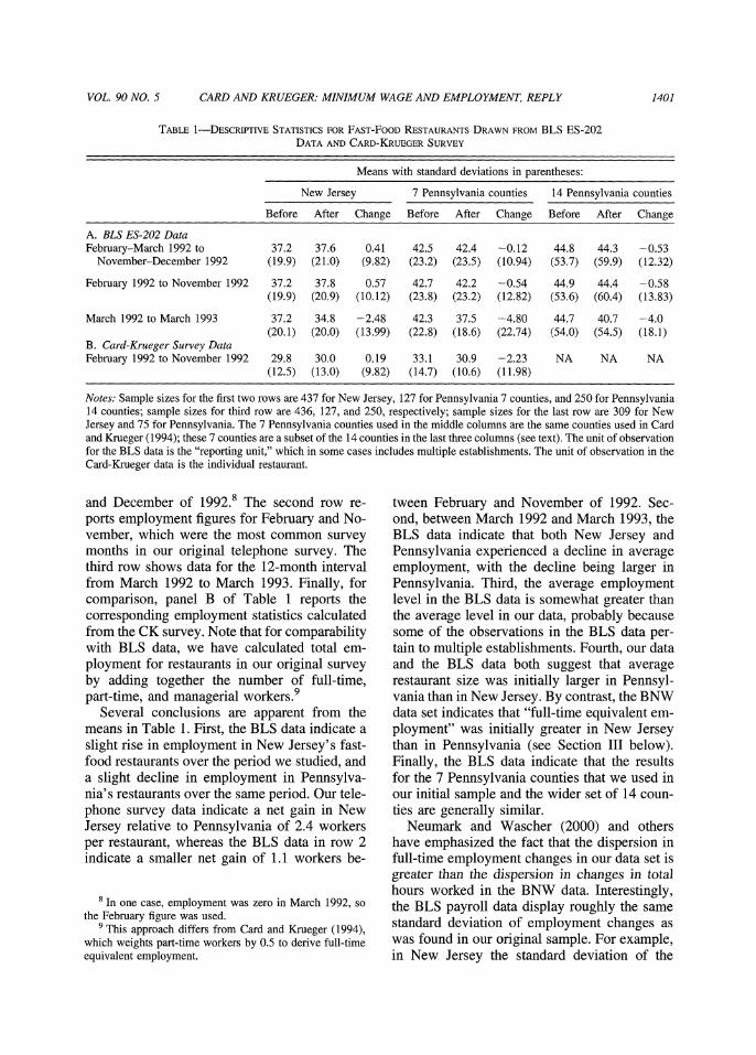
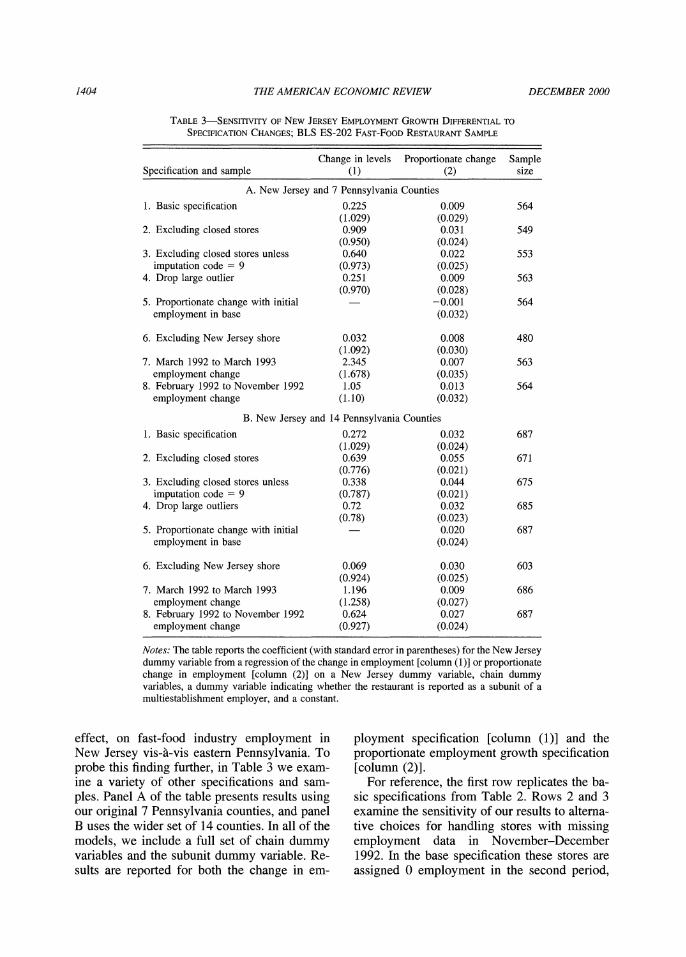
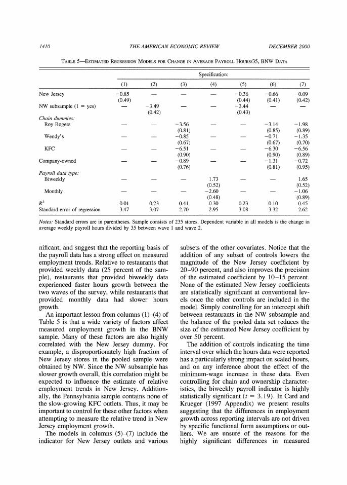
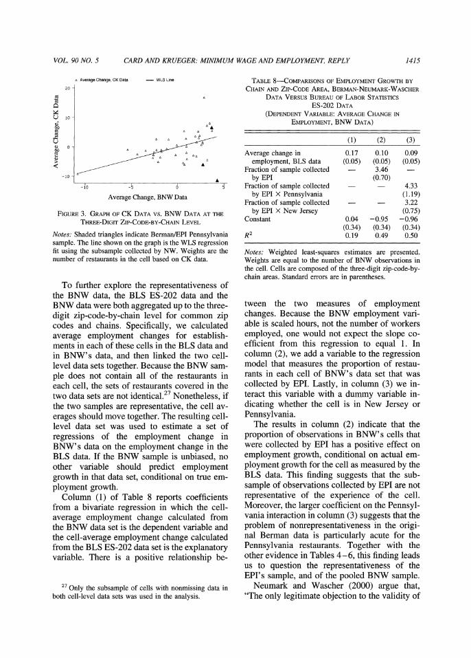
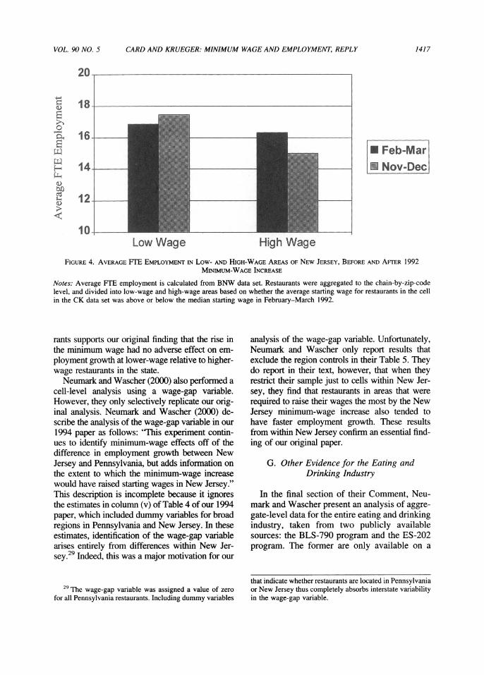Minimum Wages and Employment A Case Study of the Fast-Food Industry in New Jersey and Pennsylvania Reply

Replication and reanalysis are important en- deavors in economics especially when new find- inns run counter to conventional wisdom In their u

Comment on our 1994 American Economic Re- view article David Neumark and William Was- cher (2000) challenge our conclusion that the April 1992 increase in the New Jersey minimum wage led to no loss of employment in the fast-food industry Using data drawn from payroll records for a set of restaurants initially assembled by Rich- ard Berman of the Employment Policies Institute (EPI) and later supplemented by their own data- collection efforts Neumark and Wascher (hereaf- ter NW) conclude that the New Jersey minimum-wage increase led to a relative decline in fast-food employment in New Jersey com-pared to ~enns~1vanial They attribute the discrep- ancies between their findings and ours to problems in our fast-food restaurant data set Specifically they argue that our use of employment data derived from telephone surveys rather than from

Card Department of Economics Evans Hall Univer- sity of California Berkeley CA 94720 and National Bu- reau of Economic Research Krueger Department of Economics Princeton University Princeton NJ 08544 and National Bureau of Economic Research The analysis in Sections I 11and In subsection E of this paper is based on confidential Bureau of Labor Statistics (BLS) ES-202 data The authors thank the BLS staff for assistance with these data Although the BLS data are confidential persons employed by an eligible organization may apply to BLS for restricted access to ES-202 data for statistical research purposes Data from our 1994 paper are available via anony- mous FTP from the minimum directory of irsprincetonedu All opinions and analysis in this paper reflect the views of the authors and not the US government We thank seminar participants at Princeton University the National Bureau of Economic Research the University of Pennsylvania the University of California-Berkeley the Kennedy School (Harvard University) and Lany Katz and John Kennan for helpful comments and the Princeton University Industrial Relations Section for research support

In the March 1995 version of their paper NW relied exclusively on 71 observations collected by EPI Subse- quent versions have also included information from their supplemental data collection

payroll records led us to draw faulty inferences about the effect of the New Jersey minimum wane

u

In this paper we attempt to reconcile the contrasting findings by analyzing administrative employment data from a new representative sample of fast-food employers in New Jersey and Pennsylvania and by reanalyzing NWs data Most importantly we use the Bureau of Labor Statisticss (BLSs) employer-reported ES-202 data file to examine employment growth of fast-food restaurants in a set of major chains in New Jersey and nearby counties of ~ e n n s ~ l v a n i a ~We draw two samples from the ES-202 files a longitudinal file that tracks a fixed sample of establishments between 1992 and 1993 and a series of repeated cross sections from the end of 1991 through 1997 Because the BLS data are derived from unemployment-insurance (UI) payroll-tax records the employment measures are free of the kinds of survey errors that NW allege affected our earlier results In addition because the ES-202 data include information for all covered employers in a fixed group of restaurant chains there is no reason to doubt the representativeness of the BLS sample

A comparison of fast-food employment growth in New Jersey and Pennsylvania over the period of our original study confirms the key findings in our 1994 paper and calls into question the representativeness of the sample assembled by Berman Neumark and Wascher Consistent with our original sample the BLS fast-food data set indicates slightly faster employment growth in New Jersey than in the Pennsylvania border counties over the time period that we initially examined although in most specifications the differential is small and statistically insignificant We also use the BLS

The ES-202 data are also known as the Business Es- tablishment List






















Original 7 Cwnties



1



















372 (199)

372 (199)

372 (201)

298 (125)




















Dependent variable















































































2 NW subsample



175 175 -01 151 159 08 (55) (59) (34) (40) (59) (35) 177 167 -10 134 124 -10 (61) (63) (33) (38) (49) (35) 171 193 21 169 204 34 (35) (43) (27) (34) (43) (21)

248 284 36 290 313 22 (60) (68) (30) (55) (68) (47)






B Basic Results
















Specification

(1) (2) (3) (4) (5) (6) (7)

New Jersey -085 - - - -036 -066 -009 (049) (044) (041) (042)

NW subsample (1 = yes) - -349 - - -344 - -


Roy Rogers - - -356 - - -314 -198 (081) (085) (089)

Wendys - - -085 - - -071 - 135 (067) (067) (070)

KFC - - -651 - - -630 -656 (090) (090) (089)

Company-owned - - -089 - - -131 -072 (076) (081) (095)


(052) (052) Monthly - - - -260 - - -106




























5 No controls























Intercept -032 041 -391 (056) (050) (177)




Intercept -026 036 -352 (054) (051) (167)









2o 1

I A -10 5 d 5











EMPLOYMENTBNW DATA)





Constant












(1) AE = -200 + 1798 GAP R2=009 (111) (975)


(2) AE = 077 + 1200 GAP (078) (576)





Low Wage High Wage
















New Jersey -005 -038 -041 025 021 (095) (095) (080) (096) (072)


R~ 015 013 038 014 05 1
















IV Conclusion






u


REFERENCES















[Footnotes]



References



httpwwwjstororg
























Original 7 Cwnties



1



















372 (199)

372 (199)

372 (201)

298 (125)




















Dependent variable















































































2 NW subsample



175 175 -01 151 159 08 (55) (59) (34) (40) (59) (35) 177 167 -10 134 124 -10 (61) (63) (33) (38) (49) (35) 171 193 21 169 204 34 (35) (43) (27) (34) (43) (21)

248 284 36 290 313 22 (60) (68) (30) (55) (68) (47)






B Basic Results
















Specification

(1) (2) (3) (4) (5) (6) (7)

New Jersey -085 - - - -036 -066 -009 (049) (044) (041) (042)

NW subsample (1 = yes) - -349 - - -344 - -


Roy Rogers - - -356 - - -314 -198 (081) (085) (089)

Wendys - - -085 - - -071 - 135 (067) (067) (070)

KFC - - -651 - - -630 -656 (090) (090) (089)

Company-owned - - -089 - - -131 -072 (076) (081) (095)


(052) (052) Monthly - - - -260 - - -106




























5 No controls























Intercept -032 041 -391 (056) (050) (177)




Intercept -026 036 -352 (054) (051) (167)









2o 1

I A -10 5 d 5











EMPLOYMENTBNW DATA)





Constant












(1) AE = -200 + 1798 GAP R2=009 (111) (975)


(2) AE = 077 + 1200 GAP (078) (576)





Low Wage High Wage
















New Jersey -005 -038 -041 025 021 (095) (095) (080) (096) (072)


R~ 015 013 038 014 05 1
















IV Conclusion






u


REFERENCES















[Footnotes]



References



httpwwwjstororg














Original 7 Cwnties



1



















372 (199)

372 (199)

372 (201)

298 (125)




















Dependent variable















































































2 NW subsample



175 175 -01 151 159 08 (55) (59) (34) (40) (59) (35) 177 167 -10 134 124 -10 (61) (63) (33) (38) (49) (35) 171 193 21 169 204 34 (35) (43) (27) (34) (43) (21)

248 284 36 290 313 22 (60) (68) (30) (55) (68) (47)






B Basic Results
















Specification

(1) (2) (3) (4) (5) (6) (7)

New Jersey -085 - - - -036 -066 -009 (049) (044) (041) (042)

NW subsample (1 = yes) - -349 - - -344 - -


Roy Rogers - - -356 - - -314 -198 (081) (085) (089)

Wendys - - -085 - - -071 - 135 (067) (067) (070)

KFC - - -651 - - -630 -656 (090) (090) (089)

Company-owned - - -089 - - -131 -072 (076) (081) (095)


(052) (052) Monthly - - - -260 - - -106




























5 No controls























Intercept -032 041 -391 (056) (050) (177)




Intercept -026 036 -352 (054) (051) (167)









2o 1

I A -10 5 d 5











EMPLOYMENTBNW DATA)





Constant












(1) AE = -200 + 1798 GAP R2=009 (111) (975)


(2) AE = 077 + 1200 GAP (078) (576)





Low Wage High Wage
















New Jersey -005 -038 -041 025 021 (095) (095) (080) (096) (072)


R~ 015 013 038 014 05 1
















IV Conclusion






u


REFERENCES















[Footnotes]



References



httpwwwjstororg




Original 7 Cwnties



1



















372 (199)

372 (199)

372 (201)

298 (125)




















Dependent variable















































































2 NW subsample



175 175 -01 151 159 08 (55) (59) (34) (40) (59) (35) 177 167 -10 134 124 -10 (61) (63) (33) (38) (49) (35) 171 193 21 169 204 34 (35) (43) (27) (34) (43) (21)

248 284 36 290 313 22 (60) (68) (30) (55) (68) (47)






B Basic Results
















Specification

(1) (2) (3) (4) (5) (6) (7)

New Jersey -085 - - - -036 -066 -009 (049) (044) (041) (042)

NW subsample (1 = yes) - -349 - - -344 - -


Roy Rogers - - -356 - - -314 -198 (081) (085) (089)

Wendys - - -085 - - -071 - 135 (067) (067) (070)

KFC - - -651 - - -630 -656 (090) (090) (089)

Company-owned - - -089 - - -131 -072 (076) (081) (095)


(052) (052) Monthly - - - -260 - - -106




























5 No controls























Intercept -032 041 -391 (056) (050) (177)




Intercept -026 036 -352 (054) (051) (167)









2o 1

I A -10 5 d 5











EMPLOYMENTBNW DATA)





Constant












(1) AE = -200 + 1798 GAP R2=009 (111) (975)


(2) AE = 077 + 1200 GAP (078) (576)





Low Wage High Wage
















New Jersey -005 -038 -041 025 021 (095) (095) (080) (096) (072)


R~ 015 013 038 014 05 1
















IV Conclusion






u


REFERENCES















[Footnotes]



References



httpwwwjstororg














372 (199)

372 (199)

372 (201)

298 (125)




















Dependent variable















































































2 NW subsample



175 175 -01 151 159 08 (55) (59) (34) (40) (59) (35) 177 167 -10 134 124 -10 (61) (63) (33) (38) (49) (35) 171 193 21 169 204 34 (35) (43) (27) (34) (43) (21)

248 284 36 290 313 22 (60) (68) (30) (55) (68) (47)






B Basic Results
















Specification

(1) (2) (3) (4) (5) (6) (7)

New Jersey -085 - - - -036 -066 -009 (049) (044) (041) (042)

NW subsample (1 = yes) - -349 - - -344 - -


Roy Rogers - - -356 - - -314 -198 (081) (085) (089)

Wendys - - -085 - - -071 - 135 (067) (067) (070)

KFC - - -651 - - -630 -656 (090) (090) (089)

Company-owned - - -089 - - -131 -072 (076) (081) (095)


(052) (052) Monthly - - - -260 - - -106




























5 No controls























Intercept -032 041 -391 (056) (050) (177)




Intercept -026 036 -352 (054) (051) (167)









2o 1

I A -10 5 d 5











EMPLOYMENTBNW DATA)





Constant












(1) AE = -200 + 1798 GAP R2=009 (111) (975)


(2) AE = 077 + 1200 GAP (078) (576)





Low Wage High Wage
















New Jersey -005 -038 -041 025 021 (095) (095) (080) (096) (072)


R~ 015 013 038 014 05 1
















IV Conclusion






u


REFERENCES















[Footnotes]



References



httpwwwjstororg















Dependent variable















































































2 NW subsample



175 175 -01 151 159 08 (55) (59) (34) (40) (59) (35) 177 167 -10 134 124 -10 (61) (63) (33) (38) (49) (35) 171 193 21 169 204 34 (35) (43) (27) (34) (43) (21)

248 284 36 290 313 22 (60) (68) (30) (55) (68) (47)






B Basic Results
















Specification

(1) (2) (3) (4) (5) (6) (7)

New Jersey -085 - - - -036 -066 -009 (049) (044) (041) (042)

NW subsample (1 = yes) - -349 - - -344 - -


Roy Rogers - - -356 - - -314 -198 (081) (085) (089)

Wendys - - -085 - - -071 - 135 (067) (067) (070)

KFC - - -651 - - -630 -656 (090) (090) (089)

Company-owned - - -089 - - -131 -072 (076) (081) (095)


(052) (052) Monthly - - - -260 - - -106




























5 No controls























Intercept -032 041 -391 (056) (050) (177)




Intercept -026 036 -352 (054) (051) (167)









2o 1

I A -10 5 d 5











EMPLOYMENTBNW DATA)





Constant












(1) AE = -200 + 1798 GAP R2=009 (111) (975)


(2) AE = 077 + 1200 GAP (078) (576)





Low Wage High Wage
















New Jersey -005 -038 -041 025 021 (095) (095) (080) (096) (072)


R~ 015 013 038 014 05 1
















IV Conclusion






u


REFERENCES















[Footnotes]



References



httpwwwjstororg





Dependent variable















































































2 NW subsample



175 175 -01 151 159 08 (55) (59) (34) (40) (59) (35) 177 167 -10 134 124 -10 (61) (63) (33) (38) (49) (35) 171 193 21 169 204 34 (35) (43) (27) (34) (43) (21)

248 284 36 290 313 22 (60) (68) (30) (55) (68) (47)






B Basic Results
















Specification

(1) (2) (3) (4) (5) (6) (7)

New Jersey -085 - - - -036 -066 -009 (049) (044) (041) (042)

NW subsample (1 = yes) - -349 - - -344 - -


Roy Rogers - - -356 - - -314 -198 (081) (085) (089)

Wendys - - -085 - - -071 - 135 (067) (067) (070)

KFC - - -651 - - -630 -656 (090) (090) (089)

Company-owned - - -089 - - -131 -072 (076) (081) (095)


(052) (052) Monthly - - - -260 - - -106




























5 No controls























Intercept -032 041 -391 (056) (050) (177)




Intercept -026 036 -352 (054) (051) (167)









2o 1

I A -10 5 d 5











EMPLOYMENTBNW DATA)





Constant












(1) AE = -200 + 1798 GAP R2=009 (111) (975)


(2) AE = 077 + 1200 GAP (078) (576)





Low Wage High Wage
















New Jersey -005 -038 -041 025 021 (095) (095) (080) (096) (072)


R~ 015 013 038 014 05 1
















IV Conclusion






u


REFERENCES















[Footnotes]



References



httpwwwjstororg































































2 NW subsample



175 175 -01 151 159 08 (55) (59) (34) (40) (59) (35) 177 167 -10 134 124 -10 (61) (63) (33) (38) (49) (35) 171 193 21 169 204 34 (35) (43) (27) (34) (43) (21)

248 284 36 290 313 22 (60) (68) (30) (55) (68) (47)






B Basic Results
















Specification

(1) (2) (3) (4) (5) (6) (7)

New Jersey -085 - - - -036 -066 -009 (049) (044) (041) (042)

NW subsample (1 = yes) - -349 - - -344 - -


Roy Rogers - - -356 - - -314 -198 (081) (085) (089)

Wendys - - -085 - - -071 - 135 (067) (067) (070)

KFC - - -651 - - -630 -656 (090) (090) (089)

Company-owned - - -089 - - -131 -072 (076) (081) (095)


(052) (052) Monthly - - - -260 - - -106




























5 No controls























Intercept -032 041 -391 (056) (050) (177)




Intercept -026 036 -352 (054) (051) (167)









2o 1

I A -10 5 d 5











EMPLOYMENTBNW DATA)





Constant












(1) AE = -200 + 1798 GAP R2=009 (111) (975)


(2) AE = 077 + 1200 GAP (078) (576)





Low Wage High Wage
















New Jersey -005 -038 -041 025 021 (095) (095) (080) (096) (072)


R~ 015 013 038 014 05 1
















IV Conclusion






u


REFERENCES















[Footnotes]



References



httpwwwjstororg








































2 NW subsample



175 175 -01 151 159 08 (55) (59) (34) (40) (59) (35) 177 167 -10 134 124 -10 (61) (63) (33) (38) (49) (35) 171 193 21 169 204 34 (35) (43) (27) (34) (43) (21)

248 284 36 290 313 22 (60) (68) (30) (55) (68) (47)






B Basic Results
















Specification

(1) (2) (3) (4) (5) (6) (7)

New Jersey -085 - - - -036 -066 -009 (049) (044) (041) (042)

NW subsample (1 = yes) - -349 - - -344 - -


Roy Rogers - - -356 - - -314 -198 (081) (085) (089)

Wendys - - -085 - - -071 - 135 (067) (067) (070)

KFC - - -651 - - -630 -656 (090) (090) (089)

Company-owned - - -089 - - -131 -072 (076) (081) (095)


(052) (052) Monthly - - - -260 - - -106




























5 No controls























Intercept -032 041 -391 (056) (050) (177)




Intercept -026 036 -352 (054) (051) (167)









2o 1

I A -10 5 d 5











EMPLOYMENTBNW DATA)





Constant












(1) AE = -200 + 1798 GAP R2=009 (111) (975)


(2) AE = 077 + 1200 GAP (078) (576)





Low Wage High Wage
















New Jersey -005 -038 -041 025 021 (095) (095) (080) (096) (072)


R~ 015 013 038 014 05 1
















IV Conclusion






u


REFERENCES















[Footnotes]



References



httpwwwjstororg





























2 NW subsample



175 175 -01 151 159 08 (55) (59) (34) (40) (59) (35) 177 167 -10 134 124 -10 (61) (63) (33) (38) (49) (35) 171 193 21 169 204 34 (35) (43) (27) (34) (43) (21)

248 284 36 290 313 22 (60) (68) (30) (55) (68) (47)






B Basic Results
















Specification

(1) (2) (3) (4) (5) (6) (7)

New Jersey -085 - - - -036 -066 -009 (049) (044) (041) (042)

NW subsample (1 = yes) - -349 - - -344 - -


Roy Rogers - - -356 - - -314 -198 (081) (085) (089)

Wendys - - -085 - - -071 - 135 (067) (067) (070)

KFC - - -651 - - -630 -656 (090) (090) (089)

Company-owned - - -089 - - -131 -072 (076) (081) (095)


(052) (052) Monthly - - - -260 - - -106




























5 No controls























Intercept -032 041 -391 (056) (050) (177)




Intercept -026 036 -352 (054) (051) (167)









2o 1

I A -10 5 d 5











EMPLOYMENTBNW DATA)





Constant












(1) AE = -200 + 1798 GAP R2=009 (111) (975)


(2) AE = 077 + 1200 GAP (078) (576)





Low Wage High Wage
















New Jersey -005 -038 -041 025 021 (095) (095) (080) (096) (072)


R~ 015 013 038 014 05 1
















IV Conclusion






u


REFERENCES















[Footnotes]



References



httpwwwjstororg





















2 NW subsample



175 175 -01 151 159 08 (55) (59) (34) (40) (59) (35) 177 167 -10 134 124 -10 (61) (63) (33) (38) (49) (35) 171 193 21 169 204 34 (35) (43) (27) (34) (43) (21)

248 284 36 290 313 22 (60) (68) (30) (55) (68) (47)






B Basic Results
















Specification

(1) (2) (3) (4) (5) (6) (7)

New Jersey -085 - - - -036 -066 -009 (049) (044) (041) (042)

NW subsample (1 = yes) - -349 - - -344 - -


Roy Rogers - - -356 - - -314 -198 (081) (085) (089)

Wendys - - -085 - - -071 - 135 (067) (067) (070)

KFC - - -651 - - -630 -656 (090) (090) (089)

Company-owned - - -089 - - -131 -072 (076) (081) (095)


(052) (052) Monthly - - - -260 - - -106




























5 No controls























Intercept -032 041 -391 (056) (050) (177)




Intercept -026 036 -352 (054) (051) (167)









2o 1

I A -10 5 d 5











EMPLOYMENTBNW DATA)





Constant












(1) AE = -200 + 1798 GAP R2=009 (111) (975)


(2) AE = 077 + 1200 GAP (078) (576)





Low Wage High Wage
















New Jersey -005 -038 -041 025 021 (095) (095) (080) (096) (072)


R~ 015 013 038 014 05 1
















IV Conclusion






u


REFERENCES















[Footnotes]



References



httpwwwjstororg









2 NW subsample



175 175 -01 151 159 08 (55) (59) (34) (40) (59) (35) 177 167 -10 134 124 -10 (61) (63) (33) (38) (49) (35) 171 193 21 169 204 34 (35) (43) (27) (34) (43) (21)

248 284 36 290 313 22 (60) (68) (30) (55) (68) (47)






B Basic Results
















Specification

(1) (2) (3) (4) (5) (6) (7)

New Jersey -085 - - - -036 -066 -009 (049) (044) (041) (042)

NW subsample (1 = yes) - -349 - - -344 - -


Roy Rogers - - -356 - - -314 -198 (081) (085) (089)

Wendys - - -085 - - -071 - 135 (067) (067) (070)

KFC - - -651 - - -630 -656 (090) (090) (089)

Company-owned - - -089 - - -131 -072 (076) (081) (095)


(052) (052) Monthly - - - -260 - - -106




























5 No controls























Intercept -032 041 -391 (056) (050) (177)




Intercept -026 036 -352 (054) (051) (167)









2o 1

I A -10 5 d 5











EMPLOYMENTBNW DATA)





Constant












(1) AE = -200 + 1798 GAP R2=009 (111) (975)


(2) AE = 077 + 1200 GAP (078) (576)





Low Wage High Wage
















New Jersey -005 -038 -041 025 021 (095) (095) (080) (096) (072)


R~ 015 013 038 014 05 1
















IV Conclusion






u


REFERENCES















[Footnotes]



References



httpwwwjstororg
















Specification

(1) (2) (3) (4) (5) (6) (7)

New Jersey -085 - - - -036 -066 -009 (049) (044) (041) (042)

NW subsample (1 = yes) - -349 - - -344 - -


Roy Rogers - - -356 - - -314 -198 (081) (085) (089)

Wendys - - -085 - - -071 - 135 (067) (067) (070)

KFC - - -651 - - -630 -656 (090) (090) (089)

Company-owned - - -089 - - -131 -072 (076) (081) (095)


(052) (052) Monthly - - - -260 - - -106




























5 No controls























Intercept -032 041 -391 (056) (050) (177)




Intercept -026 036 -352 (054) (051) (167)









2o 1

I A -10 5 d 5











EMPLOYMENTBNW DATA)





Constant












(1) AE = -200 + 1798 GAP R2=009 (111) (975)


(2) AE = 077 + 1200 GAP (078) (576)





Low Wage High Wage
















New Jersey -005 -038 -041 025 021 (095) (095) (080) (096) (072)


R~ 015 013 038 014 05 1
















IV Conclusion






u


REFERENCES















[Footnotes]



References



httpwwwjstororg





Specification

(1) (2) (3) (4) (5) (6) (7)

New Jersey -085 - - - -036 -066 -009 (049) (044) (041) (042)

NW subsample (1 = yes) - -349 - - -344 - -


Roy Rogers - - -356 - - -314 -198 (081) (085) (089)

Wendys - - -085 - - -071 - 135 (067) (067) (070)

KFC - - -651 - - -630 -656 (090) (090) (089)

Company-owned - - -089 - - -131 -072 (076) (081) (095)


(052) (052) Monthly - - - -260 - - -106




























5 No controls























Intercept -032 041 -391 (056) (050) (177)




Intercept -026 036 -352 (054) (051) (167)









2o 1

I A -10 5 d 5











EMPLOYMENTBNW DATA)





Constant












(1) AE = -200 + 1798 GAP R2=009 (111) (975)


(2) AE = 077 + 1200 GAP (078) (576)





Low Wage High Wage
















New Jersey -005 -038 -041 025 021 (095) (095) (080) (096) (072)


R~ 015 013 038 014 05 1
















IV Conclusion






u


REFERENCES















[Footnotes]



References



httpwwwjstororg























5 No controls























Intercept -032 041 -391 (056) (050) (177)




Intercept -026 036 -352 (054) (051) (167)









2o 1

I A -10 5 d 5











EMPLOYMENTBNW DATA)





Constant












(1) AE = -200 + 1798 GAP R2=009 (111) (975)


(2) AE = 077 + 1200 GAP (078) (576)





Low Wage High Wage
















New Jersey -005 -038 -041 025 021 (095) (095) (080) (096) (072)


R~ 015 013 038 014 05 1
















IV Conclusion






u


REFERENCES















[Footnotes]



References



httpwwwjstororg












5 No controls























Intercept -032 041 -391 (056) (050) (177)




Intercept -026 036 -352 (054) (051) (167)









2o 1

I A -10 5 d 5











EMPLOYMENTBNW DATA)





Constant












(1) AE = -200 + 1798 GAP R2=009 (111) (975)


(2) AE = 077 + 1200 GAP (078) (576)





Low Wage High Wage
















New Jersey -005 -038 -041 025 021 (095) (095) (080) (096) (072)


R~ 015 013 038 014 05 1
















IV Conclusion






u


REFERENCES















[Footnotes]



References



httpwwwjstororg

















Intercept -032 041 -391 (056) (050) (177)




Intercept -026 036 -352 (054) (051) (167)









2o 1

I A -10 5 d 5











EMPLOYMENTBNW DATA)





Constant












(1) AE = -200 + 1798 GAP R2=009 (111) (975)


(2) AE = 077 + 1200 GAP (078) (576)





Low Wage High Wage
















New Jersey -005 -038 -041 025 021 (095) (095) (080) (096) (072)


R~ 015 013 038 014 05 1
















IV Conclusion






u


REFERENCES















[Footnotes]



References



httpwwwjstororg







Intercept -032 041 -391 (056) (050) (177)




Intercept -026 036 -352 (054) (051) (167)









2o 1

I A -10 5 d 5











EMPLOYMENTBNW DATA)





Constant












(1) AE = -200 + 1798 GAP R2=009 (111) (975)


(2) AE = 077 + 1200 GAP (078) (576)





Low Wage High Wage
















New Jersey -005 -038 -041 025 021 (095) (095) (080) (096) (072)


R~ 015 013 038 014 05 1
















IV Conclusion






u


REFERENCES















[Footnotes]



References



httpwwwjstororg





2o 1

I A -10 5 d 5











EMPLOYMENTBNW DATA)





Constant












(1) AE = -200 + 1798 GAP R2=009 (111) (975)


(2) AE = 077 + 1200 GAP (078) (576)





Low Wage High Wage
















New Jersey -005 -038 -041 025 021 (095) (095) (080) (096) (072)


R~ 015 013 038 014 05 1
















IV Conclusion






u


REFERENCES















[Footnotes]



References



httpwwwjstororg










(1) AE = -200 + 1798 GAP R2=009 (111) (975)


(2) AE = 077 + 1200 GAP (078) (576)





Low Wage High Wage
















New Jersey -005 -038 -041 025 021 (095) (095) (080) (096) (072)


R~ 015 013 038 014 05 1
















IV Conclusion






u


REFERENCES















[Footnotes]



References



httpwwwjstororg




Low Wage High Wage
















New Jersey -005 -038 -041 025 021 (095) (095) (080) (096) (072)


R~ 015 013 038 014 05 1
















IV Conclusion






u


REFERENCES















[Footnotes]



References



httpwwwjstororg









New Jersey -005 -038 -041 025 021 (095) (095) (080) (096) (072)


R~ 015 013 038 014 05 1
















IV Conclusion






u


REFERENCES















[Footnotes]



References



httpwwwjstororg









IV Conclusion






u


REFERENCES















[Footnotes]



References



httpwwwjstororg





u


REFERENCES















[Footnotes]



References



httpwwwjstororg







[Footnotes]



References



httpwwwjstororg



Documents

Minimum Wages and Employment: A Case Study of the Fast ... Media... · journals and scholarly literature from ... A Case Study of the Fast-Food Industry in New Jersey ... wage led