Michael Grayling - fm

Efficient multivariate normal distribution calculations in StataMichael Grayling

Introduction ConclusionMethods Results

Efficient multivariate normal distribution calculations in Stata

Michael Grayling

Supervisor: Adrian Mander

MRC Biostatistics Unit

2015 UK Stata Users Group Meeting10/09/15

1/21

Why and what?

Why do we need to be able to work with the Multivariate Normal Distribution?



2/21

• The normal distribution has significant importance in statistics.

• Much real world data either is, or is assumed to be, normally distributed.

• Whilst the central limit theorem tells us the mean of many random variables drawn independently from the samedistribution will be approximately normally distributed.

• Today however a considerable amount of statistical analysis performed is not univariate, but multivariate in nature.

• Consequently the generalisation of the normal distribution to higher dimensions; the multivariate normaldistribution, is of increasing importance.

Why and what?

Definition


ConclusionMethods ResultsIntroduction

3/21

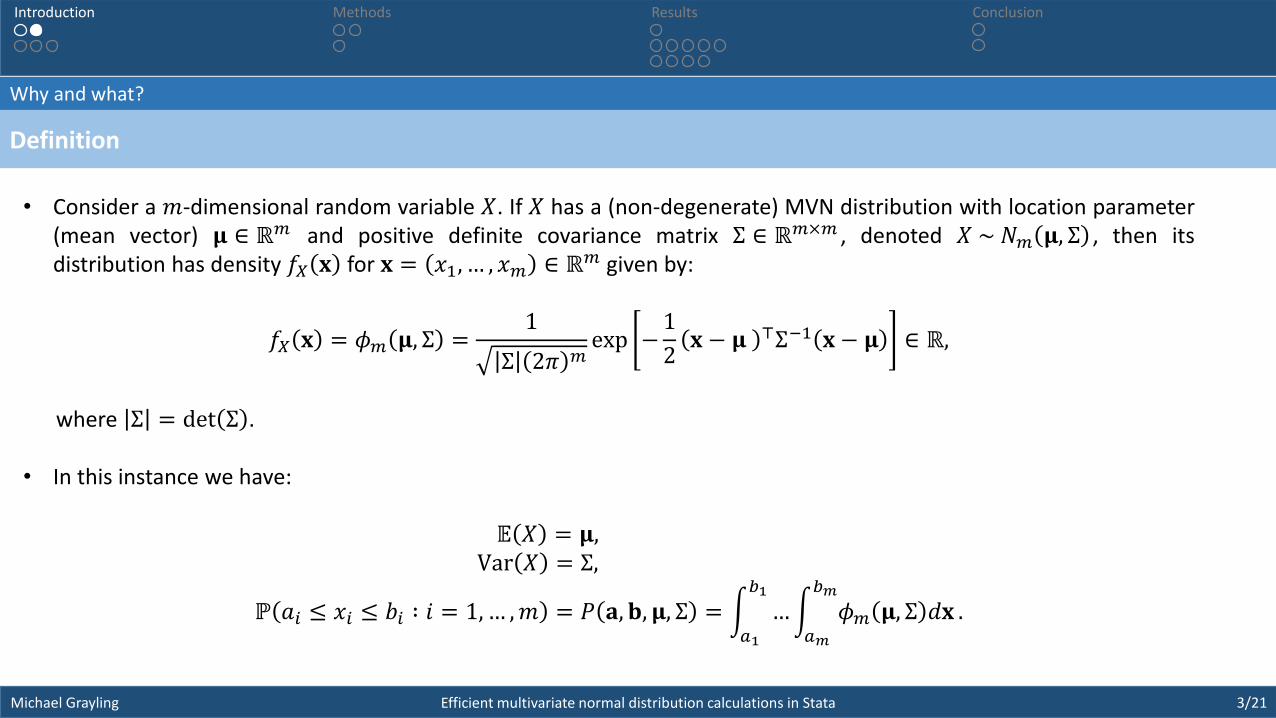
• Consider a 𝑚-dimensional random variable 𝑋. If 𝑋 has a (non-degenerate) MVN distribution with location parameter(mean vector) 𝛍 ∈ ℝ𝑚 and positive definite covariance matrix Σ ∈ ℝ𝑚×𝑚 , denoted 𝑋 ~ 𝑁𝑚 𝛍, Σ , then itsdistribution has density 𝑓𝑋 𝐱 for 𝐱 = 𝑥1, … , 𝑥𝑚 ∈ ℝ𝑚 given by:

𝑓𝑋 𝐱 = 𝜙𝑚 𝛍, Σ =1

Σ 2𝜋 𝑚exp −

1

2𝐱 − 𝛍 ⊤Σ−1 𝐱 − 𝛍 ∈ ℝ,

where Σ = det Σ .

• In this instance we have:

𝔼 𝑋 = 𝛍,Var 𝑋 = Σ,

ℙ 𝑎𝑖 ≤ 𝑥𝑖 ≤ 𝑏𝑖 ∶ 𝑖 = 1,… ,𝑚 = 𝑃 𝐚, 𝐛, 𝛍, Σ = 𝑎1

𝑏1

… 𝑎𝑚

𝑏𝑚

𝜙𝑚 𝛍, Σ 𝑑𝐱 .

The multivariate normal distribution in Stata

What’s available?



4/21

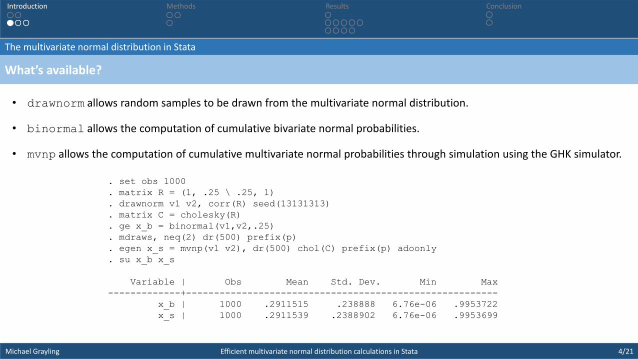
• drawnorm allows random samples to be drawn from the multivariate normal distribution.

• binormal allows the computation of cumulative bivariate normal probabilities.

• mvnp allows the computation of cumulative multivariate normal probabilities through simulation using the GHK simulator.

. set obs 1000

. matrix R = (1, .25 \ .25, 1)

. drawnorm v1 v2, corr(R) seed(13131313)

. matrix C = cholesky(R)

. ge x_b = binormal(v1,v2,.25)

. mdraws, neq(2) dr(500) prefix(p)

. egen x_s = mvnp(v1 v2), dr(500) chol(C) prefix(p) adoonly

. su x_b x_s

Variable | Obs Mean Std. Dev. Min Max

-------------+--------------------------------------------------------

x_b | 1000 .2911515 .238888 6.76e-06 .9953722

x_s | 1000 .2911539 .2388902 6.76e-06 .9953699


The new commands



5/21

• Utilise Mata and one of the new efficient algorithms that has been developed to quickly compute probabilities over any range of integration.

• Additionally, there’s currently no easy means to compute equi-coordinate quantiles which have a range of applications:

𝑝 = −∞

𝑞

… −∞

𝑞

𝜙𝑚 𝛍, Σ 𝑑𝛉,

so use interval bisection to search for 𝑞, employing the former algorithm for probabilities to evaluate the RHS.

• Final commands named mvnormalden, mvnormal, invmvnormal and rmvnormal, with all four using Mata.

• mvnormal in particular makes use of a recently developed Quasi-Monte Carlo Randomised Lattice algorithm forperforming the required integration.

• All four are easy to use with little user input required.


Talk outline



6/21

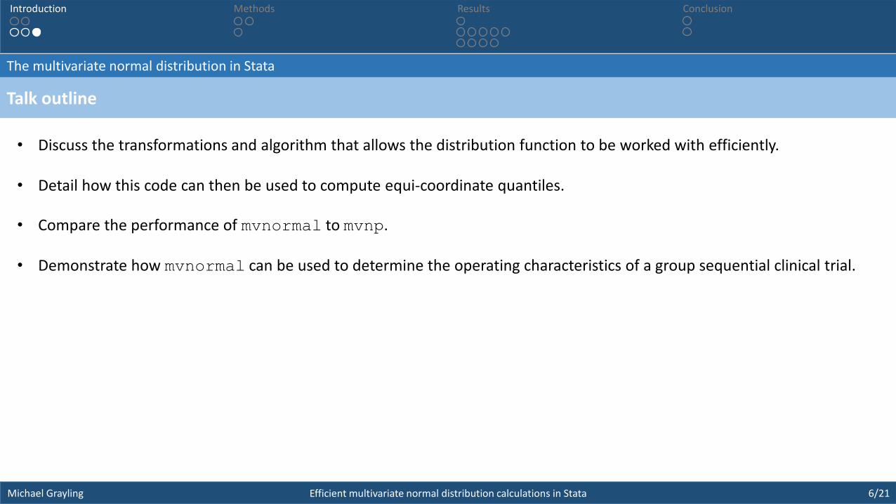
• Discuss the transformations and algorithm that allows the distribution function to be worked with efficiently.

• Detail how this code can then be used to compute equi-coordinate quantiles.

• Compare the performance of mvnormal to mvnp.

• Demonstrate how mvnormal can be used to determine the operating characteristics of a group sequential clinical trial.

Working with the distribution function

Transforming the integral



7/21

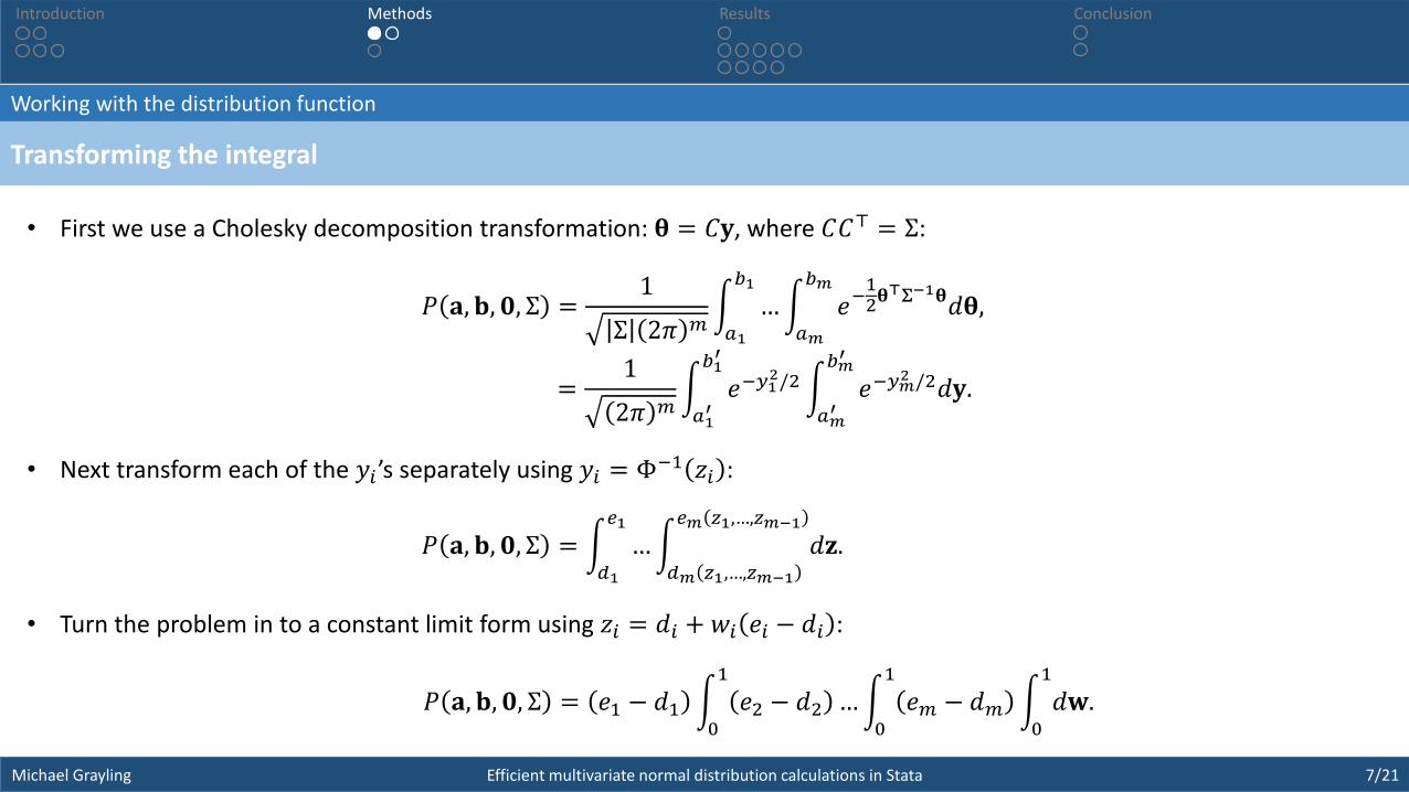
• First we use a Cholesky decomposition transformation: 𝛉 = 𝐶𝐲, where 𝐶𝐶⊤ = Σ:

𝑃 𝐚, 𝐛, 𝟎, Σ =1

Σ 2𝜋 𝑚 𝑎1

𝑏1

… 𝑎𝑚

𝑏𝑚

𝑒−12𝛉

⊤Σ−1𝛉𝑑𝛉,

, , , =1

2𝜋 𝑚 𝑎1′

𝑏1′

𝑒−𝑦12/2

𝑎𝑚′

𝑏𝑚′

𝑒−𝑦𝑚2 /2𝑑𝐲.

• Next transform each of the 𝑦𝑖’s separately using 𝑦𝑖 = Φ−1 𝑧𝑖 :

𝑃 𝐚, 𝐛, 𝟎, Σ = 𝑑1

𝑒1

… 𝑑𝑚 𝑧1,…,𝑧𝑚−1

𝑒𝑚 𝑧1,…,𝑧𝑚−1

𝑑𝐳.

• Turn the problem in to a constant limit form using 𝑧𝑖 = 𝑑𝑖 + 𝑤𝑖 𝑒𝑖 − 𝑑𝑖 :

𝑃 𝐚, 𝐛, 𝟎, Σ = 𝑒1 − 𝑑1 0

1

𝑒2 − 𝑑2 … 0

1

𝑒𝑚 − 𝑑𝑚 0

1

𝑑𝐰.

Working with the distribution function

Quasi Monte Carlo Randomised Lattice Algorithm


Introduction ConclusionResultsMethods

8/21

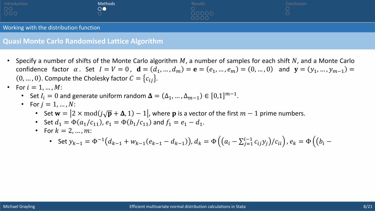
• Specify a number of shifts of the Monte Carlo algorithm 𝑀, a number of samples for each shift 𝑁, and a Monte Carloconfidence factor 𝛼 . Set 𝐼 = 𝑉 = 0 , 𝐝 = 𝑑1, … , 𝑑𝑚 = 𝐞 = 𝑒1, … , 𝑒𝑚 = 0,… , 0 and 𝐲 = 𝑦1, … , 𝑦𝑚−1 =

0,… , 0 . Compute the Cholesky factor 𝐶 = 𝑐𝑖𝑗 .

• For 𝑖 = 1,… ,𝑀:• Set 𝐼𝑖 = 0 and generate uniform random 𝚫 = Δ1, … , Δ𝑚−1 ∈ 0,1 𝑚−1.• For 𝑗 = 1,… , 𝑁:

• Set 𝐰 = 2 ×mod 𝑗 𝐩 + 𝚫, 1 − 1 , where 𝐩 is a vector of the first 𝑚 − 1 prime numbers.

• Set 𝑑1 = Φ 𝑎1/𝑐11 , 𝑒1 = Φ 𝑏1/𝑐11 and 𝑓1 = 𝑒1 − 𝑑1.• For 𝑘 = 2,… ,𝑚:

• Set 𝑦𝑘−1 = Φ−1 𝑑𝑘−1 + 𝑤𝑘−1 𝑒𝑘−1 − 𝑑𝑘−1 , 𝑑𝑘 = Φ 𝑎𝑖 − 𝑗=1𝑖−1 𝑐𝑖𝑗𝑦𝑗 /𝑐𝑖𝑖 , 𝑒𝑘 = Φ 𝑏𝑖 −

Equi-coordinate quantiles

Computing equi-coordinate quantiles


Introduction ConclusionResultsMethods

9/21

• Recall the definition of an equi-coordinate quantile:

𝑝 = 𝑓 𝑞 = −∞

𝑞

… −∞

𝑞

Φ𝑚 𝛍, Σ 𝑑𝛉.

• We can compute 𝑞 for any 𝑝 efficiently using the algorithm discussed previously to evaluate the RHS for any 𝑞, andmodified interval bisection to search for the correct 𝑞.

• Optimize does not work well because of the small errors present when you evaluate the RHS.

• Choose a maximum number of interactions 𝑖max, and a tolerance 𝜖.• Initialise 𝑎 = −106, 𝑏 = 106 and 𝑖 = 1. Compute 𝑓 𝑎 and 𝑓 𝑏 .• While 𝑖 ≤ 𝑖max:

• Set 𝑐 = 𝑎 − 𝑏 − 𝑎 / 𝑓 𝑏 − 𝑓 𝑎 𝑓 𝑎 and compute 𝑓 𝑐 .

• If 𝑓 𝑐 = 0 or 𝑏 − 𝑎 /2 < 𝜖 break. Else:• If 𝑓 𝑎 , 𝑓 𝑐 < 0 or 𝑓 𝑎 , 𝑓 𝑐 > 0 set 𝑎 = 𝑐 and 𝑓 𝑎 = 𝑓 𝑐 . Else set 𝑏 = 𝑐 and 𝑓(𝑏) = 𝑓(𝑐).

• Set 𝑖 = 𝑖 + 1.• Return 𝑞 = 𝑐.

Syntax

mvnormal



10/21

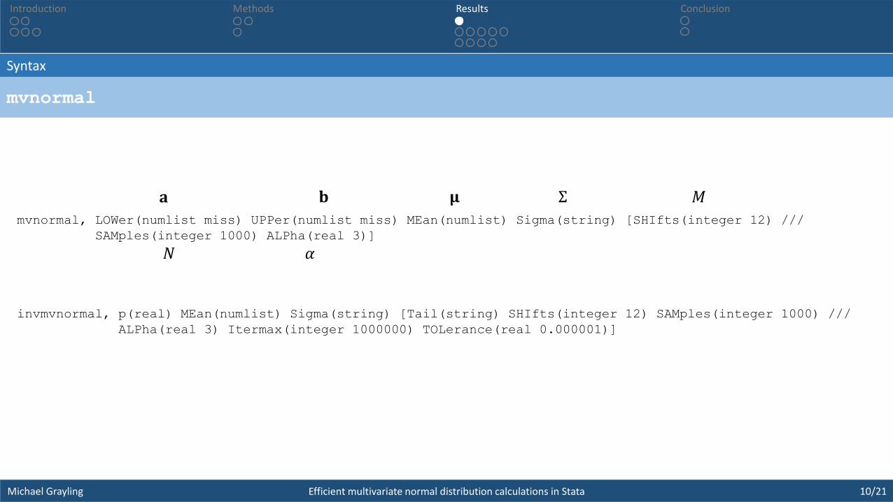
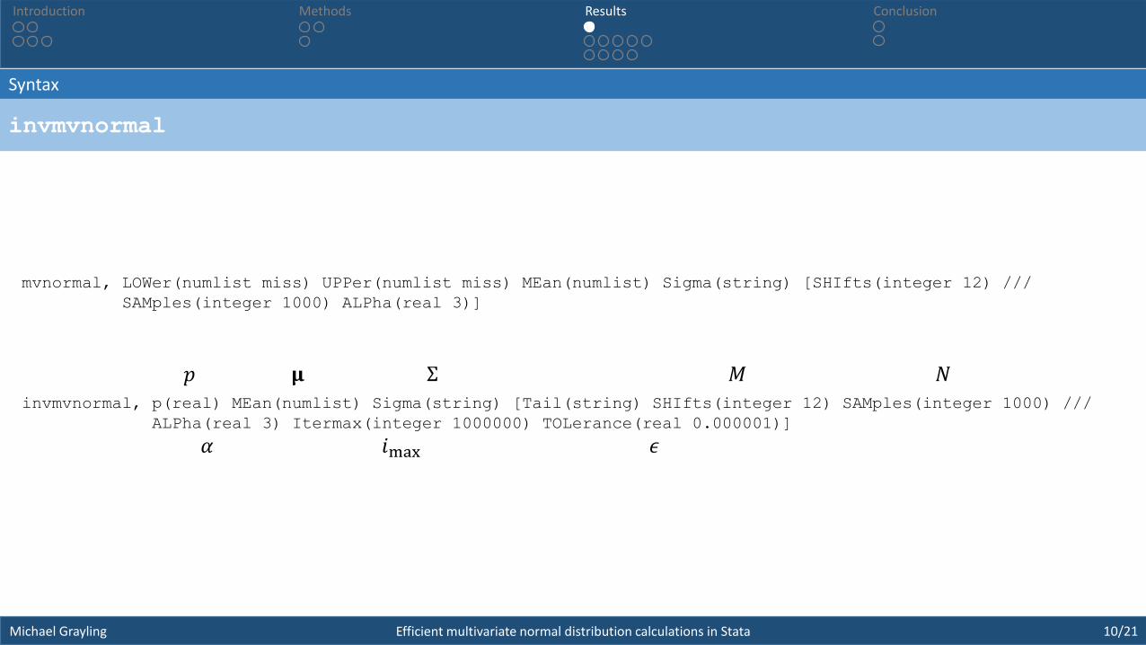
mvnormal, LOWer(numlist miss) UPPer(numlist miss) MEan(numlist) Sigma(string) [SHIfts(integer 12) ///

SAMples(integer 1000) ALPha(real 3)]

invmvnormal, p(real) MEan(numlist) Sigma(string) [Tail(string) SHIfts(integer 12) SAMples(integer 1000) ///

ALPha(real 3) Itermax(integer 1000000) TOLerance(real 0.000001)]

𝛍 Σ𝐚 𝐛

𝛼

𝑀

𝑁

Syntax

invmvnormal



10/21





𝑀 𝑁

𝑖max 𝜖

𝑝 𝛍 Σ

𝛼

Syntax

invmvnormal



10/21





𝑀 𝑁

𝑖max 𝜖

𝑝 𝛍 Σ

𝛼

lower, upper, or both

Performance Comparison

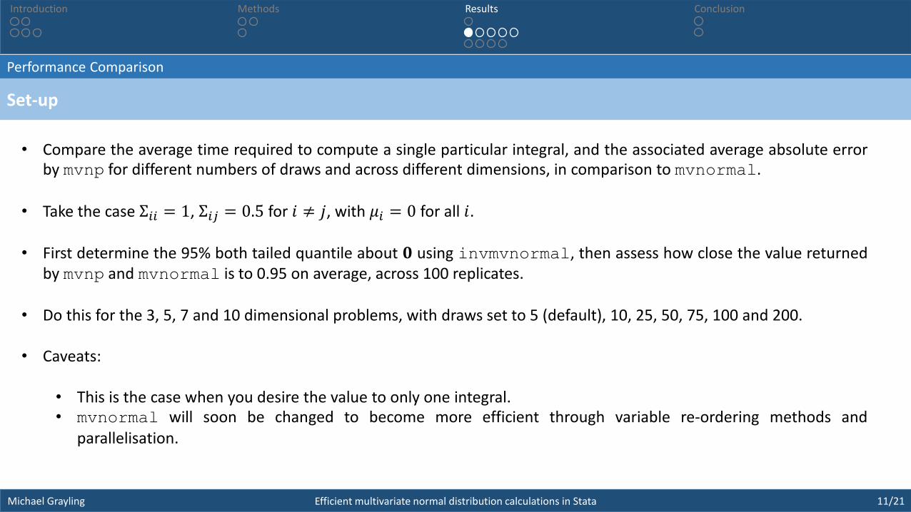
Set-up



11/21

• Compare the average time required to compute a single particular integral, and the associated average absolute errorby mvnp for different numbers of draws and across different dimensions, in comparison to mvnormal.

• Take the case Σ𝑖𝑖 = 1, Σ𝑖𝑗 = 0.5 for 𝑖 ≠ 𝑗, with 𝜇𝑖 = 0 for all 𝑖.

• First determine the 95% both tailed quantile about 𝟎 using invmvnormal, then assess how close the value returnedby mvnp and mvnormal is to 0.95 on average, across 100 replicates.

• Do this for the 3, 5, 7 and 10 dimensional problems, with draws set to 5 (default), 10, 25, 50, 75, 100 and 200.

• Caveats:

• This is the case when you desire the value to only one integral.• mvnormal will soon be changed to become more efficient through variable re-ordering methods and

parallelisation.


Using invmvnormal and mvnormal



12/21

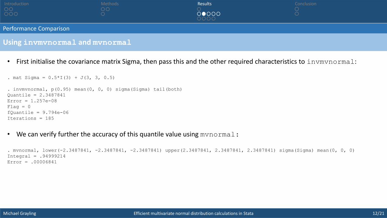
• First initialise the covariance matrix Sigma, then pass this and the other required characteristics to invmvnormal:

. mat Sigma = 0.5*I(3) + J(3, 3, 0.5)

. invmvnormal, p(0.95) mean(0, 0, 0) sigma(Sigma) tail(both)

Quantile = 2.3487841

Error = 1.257e-08

Flag = 0

fQuantile = 9.794e-06

Iterations = 185

• We can verify further the accuracy of this quantile value using mvnormal:

. mvnormal, lower(-2.3487841, -2.3487841, -2.3487841) upper(2.3487841, 2.3487841, 2.3487841) sigma(Sigma) mean(0, 0, 0)

Integral = .94999214

Error = .00006841


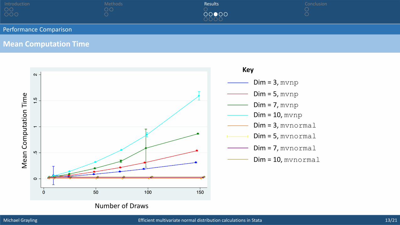
Mean Computation Time



13/21

Number of Draws

Mea

n C

om

pu

tati

on

Tim

e

Key

Dim = 3, mvnp

Dim = 5, mvnp

Dim = 7, mvnp

Dim = 10, mvnp

Dim = 3, mvnormal

Dim = 5, mvnormal

Dim = 7, mvnormal

Dim = 10, mvnormal


Mean Absolute Error



14/21

Key

Dim = 3, mvnp

Dim = 5, mvnp

Dim = 7, mvnp

Dim = 10, mvnp

Dim = 3, mvnormal

Dim = 5, mvnormal

Dim = 7, mvnormal

Dim = 10, mvnormalMea

n A

bso

lute

Err

or

Number of Draws


Relative Performance



15/21

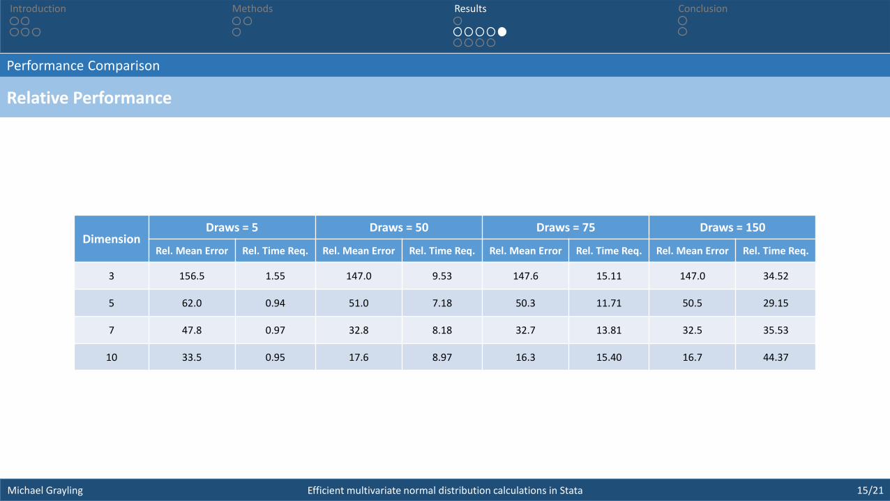
DimensionDraws = 5 Draws = 50 Draws = 75 Draws = 150

Rel. Mean Error Rel. Time Req. Rel. Mean Error Rel. Time Req. Rel. Mean Error Rel. Time Req. Rel. Mean Error Rel. Time Req.

3 156.5 1.55 147.0 9.53 147.6 15.11 147.0 34.52

5 62.0 0.94 51.0 7.18 50.3 11.71 50.5 29.15

7 47.8 0.97 32.8 8.18 32.7 13.81 32.5 35.53

10 33.5 0.95 17.6 8.97 16.3 15.40 16.7 44.37

Group sequential clinical trial design

Triangular Test



16/21

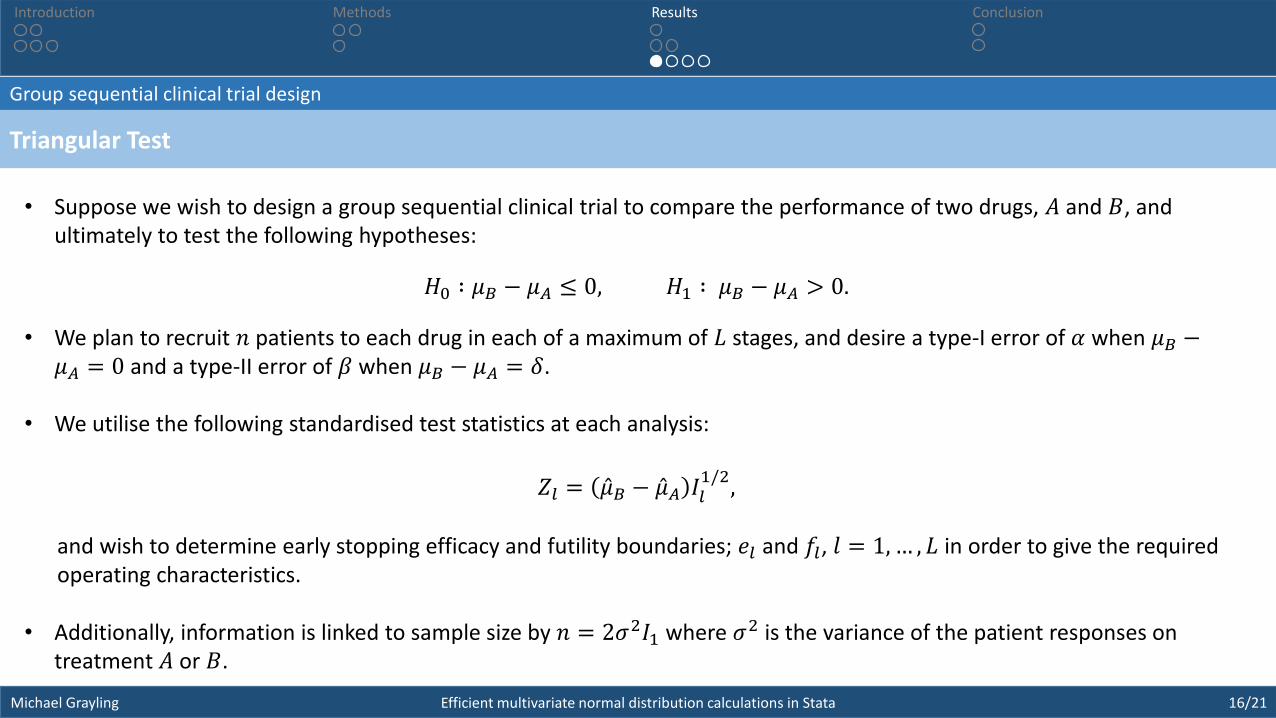
• Suppose we wish to design a group sequential clinical trial to compare the performance of two drugs, 𝐴 and 𝐵, and ultimately to test the following hypotheses:

𝐻0 ∶ 𝜇𝐵 − 𝜇𝐴 ≤ 0, 𝐻1 ∶ 𝜇𝐵 − 𝜇𝐴 > 0.

• We plan to recruit 𝑛 patients to each drug in each of a maximum of 𝐿 stages, and desire a type-I error of 𝛼 when 𝜇𝐵 −𝜇𝐴 = 0 and a type-II error of 𝛽 when 𝜇𝐵 − 𝜇𝐴 = 𝛿.

• We utilise the following standardised test statistics at each analysis:

𝑍𝑙 = 𝜇𝐵 − 𝜇𝐴 𝐼𝑙1/2

,

and wish to determine early stopping efficacy and futility boundaries; 𝑒𝑙 and 𝑓𝑙, 𝑙 = 1, … , 𝐿 in order to give the required operating characteristics.

• Additionally, information is linked to sample size by 𝑛 = 2𝜎2𝐼1 where 𝜎2 is the variance of the patient responses on treatment 𝐴 or 𝐵.


Triangular Test



17/21

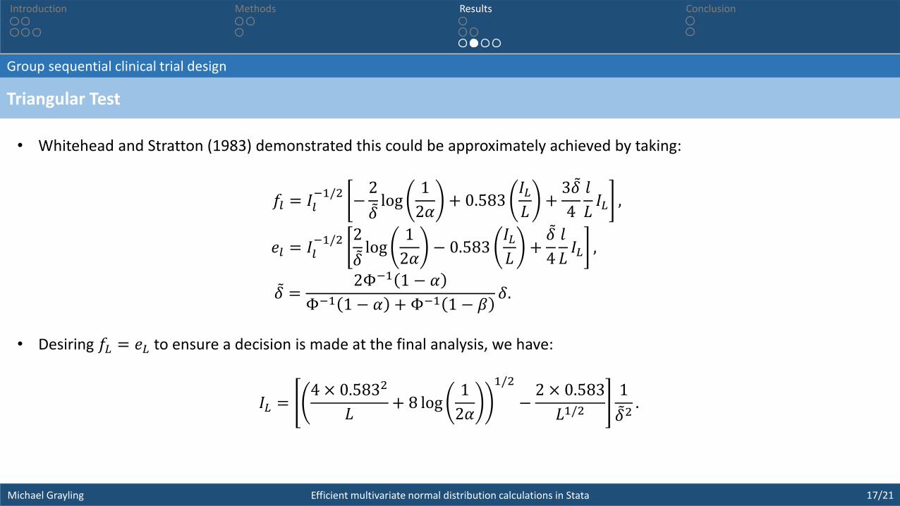
• Whitehead and Stratton (1983) demonstrated this could be approximately achieved by taking:

𝑓𝑙 = 𝐼𝑙−1/2

−2

𝛿log

1

2𝛼+ 0.583

𝐼𝐿𝐿

+3 𝛿

4

𝑙

𝐿𝐼𝐿 ,

𝑒𝑙 = 𝐼𝑙−1/2 2

𝛿log

1

2𝛼− 0.583

𝐼𝐿𝐿

+ 𝛿

4

𝑙

𝐿𝐼𝐿 ,

𝛿 =2Φ−1 1 − 𝛼

Φ−1 1 − 𝛼 + Φ−1 1 − 𝛽𝛿.

• Desiring 𝑓𝐿 = 𝑒𝐿 to ensure a decision is made at the final analysis, we have:

𝐼𝐿 =4 × 0.5832

𝐿+ 8 log

1

2𝛼

1/2

−2 × 0.583

𝐿1/21

𝛿2.


Computing the Designs Performance



18/21

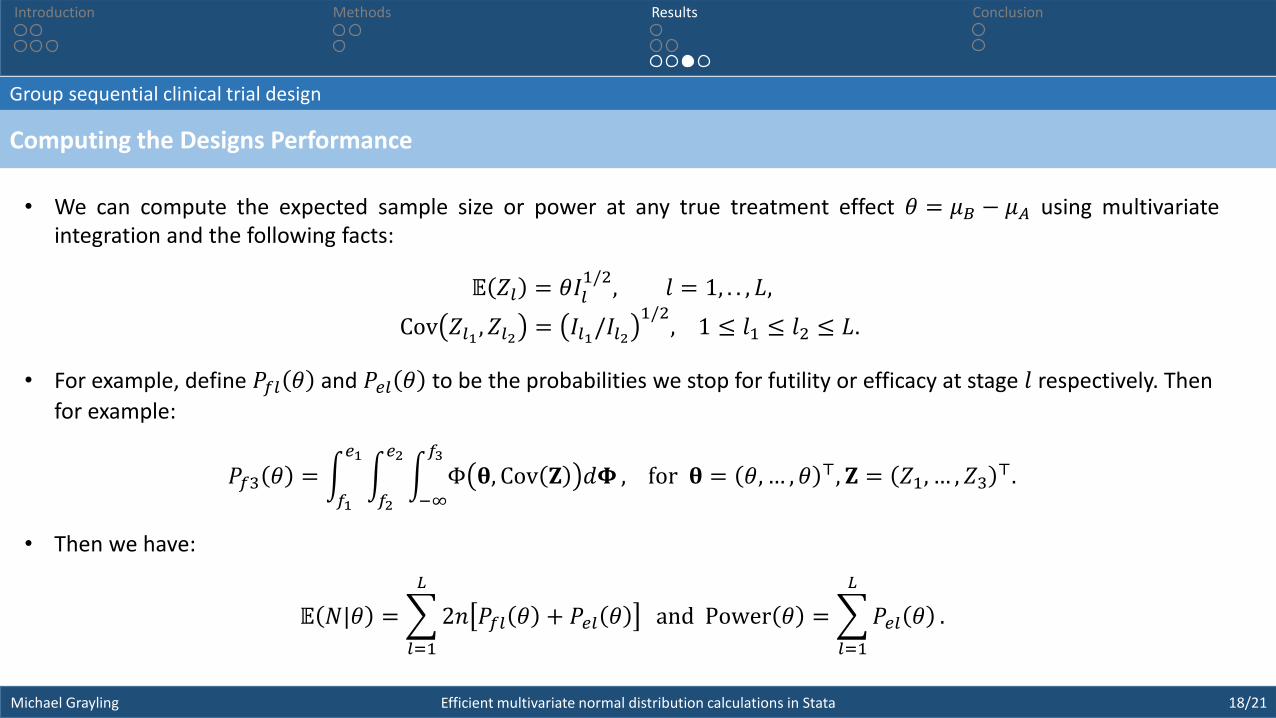
• We can compute the expected sample size or power at any true treatment effect 𝜃 = 𝜇𝐵 − 𝜇𝐴 using multivariateintegration and the following facts:

𝔼 𝑍𝑙 = 𝜃𝐼𝑙1/2

, 𝑙 = 1, . . , 𝐿,

Cov 𝑍𝑙1 , 𝑍𝑙2 = 𝐼𝑙1/𝐼𝑙21/2

, 1 ≤ 𝑙1 ≤ 𝑙2 ≤ 𝐿.

• For example, define 𝑃𝑓𝑙 𝜃 and 𝑃𝑒𝑙 𝜃 to be the probabilities we stop for futility or efficacy at stage 𝑙 respectively. Then

for example:

𝑃𝑓3 𝜃 = 𝑓1

𝑒1

𝑓2

𝑒2

−∞

𝑓3

Φ 𝛉, Cov 𝐙 𝑑𝚽 , , , for 𝛉 = 𝜃,… , 𝜃 ⊤, 𝐙 = 𝑍1, … , 𝑍3⊤.

• Then we have:

𝔼 𝑁|𝜃 =

𝑙=1

𝐿

2𝑛 𝑃𝑓𝑙 𝜃 + 𝑃𝑒𝑙 𝜃 and Power 𝜃 =

𝑙=1

𝐿

𝑃𝑒𝑙 𝜃 .


Power and expected sample size



19/21

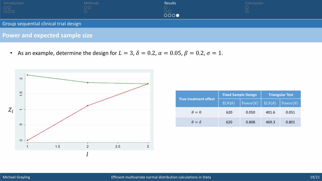
𝑍𝑙

𝑙

True treatment effectFixed Sample Design Triangular Test

𝔼 𝑁|𝜃 Power 𝜃 𝔼 𝑁|𝜃 Power 𝜃

𝜃 = 0 620 0.050 401.6 0.051

𝜃 = 𝛿 620 0.808 469.3 0.801

• As an example, determine the design for 𝐿 = 3, 𝛿 = 0.2, 𝛼 = 0.05, 𝛽 = 0.2, 𝜎 = 1.

Conclusion

Complete and simple to use



20/21

• Created four easy to use commands that allow you to work with the multivariate normal distribution.

• Performance of these commands is seen to be very good.

• Complementary to mvnp with the relative efficiency dependent on the number of required integrals.

• Similarly, we have created commands for working with the multivariate 𝑡 distribution.

• Moving forward, we would like to add functionality to allow alternate specialist algorithms to be used.

Conclusion

Questions?

Efficient multivariate normal distribution calculations in StataMichael Grayling 21/21

Introduction Methods Results Conclusion

Documents

Michael Grayling - fm