Embed Size (px)
Citation preview
AEAT/ED51014/Methodology Volume 2 Issue 1
AEA Technology Environment
Service Contract for Carrying out Cost-Benefit
Analysis of Air Quality Related Issues, in particular in the Clean Air for Europe (CAFE) Programme
Methodology for the Cost-Benefit analysis for CAFE:
Volume 2: Health Impact Assessment
February 2005
AEAT/ED51014/Methodology Volume 2: Issue 2
AEA Technology
Title Methodology Paper (Volume 2) for
Service Contract for carrying out cost-benefit analysis of air quality related issues, in particular in the clean air for Europe (CAFE) programme
Customer European Commission DG Environment Customer reference ENV.C.1/SER/2003/0027 Confidentiality, copyright and reproduction
This document has been prepared by AEA Technology plc in connection with a contract to supply goods and/or services and is submitted only on the basis of strict confidentiality. The contents must not be disclosed to third parties other than in accordance with the terms of the contract.
Validity Issue 1 File reference AEAT/ED51014/Methodology Volume 2: Issue 2 Reference number AEAT/ED51014/ Methodology Volume 2: Issue 2 AEA Technology Environment Bdg 154 Harwell Business Centre
Didcot, Oxon, OX11 0QJ United Kingdom
Telephone +44 (0) 870 190 6592 Facsimile +44 (0) 870 190 6327 Email: [email protected] AEA Technology Environment is a business division of AEA Technology plc AEA Technology Environment is certificated to ISO9001 &
ISO 14001 Name Signature Date Authors Fintan Hurley, Alistair Hunt,
Hilary Cowie, Mike Holland, Brian Miller, Stephen Pye, Paul Watkiss
24/2//2005
Reviewed by Paul Watkiss 24/2//2005 Approved by Paul Watkiss 24/2//2005
AEAT/ED51014/Methodology Volume 2: Issue 2
AEA Technology i
Executive Summary Introduction; relationship to other reports This document defines in detail the methodology used for quantification and valuation of the health impacts of ozone and particulate matter for the cost-benefit analysis (CBA) being undertaken as part of the Clean Air For Europe (CAFE) programme. An earlier version was previously released as an appendix to the draft methodology report issued by the CBA team in July 2004, though it was subsequently felt that the detailed assessment of methods for estimating health effects should be presented as a separate volume. This is partly because of the importance of health effects within the overall CBA. It is also because there is not at present an alternative detailed write-up of health endpoints, and associated concentration-response functions, background rates and health impact assessment (HIA) methodology, for estimating the benefits to health of reducing air pollution in Europe. This is not the case for (e.g.) effects of air pollution on ecosystems and crops, for which ICP/MM (Mapping and Modelling) (2004) has recently produced extensive guidance. Chapter 1 raises a wide range of general issues concerning the process of HIA in general. Chapter 2 onwards describes the substantial and main body of the HIA methodology report. It has been revised following peer review, stakeholder comment, and the opportunity for further investigation and discussion of available data. Efforts have been made to ensure consistency between our methodology and the various evaluations that the World Health Organisation (WHO) provided for CAFE. These included:
a. a comprehensive but generally qualitative review of the health effects of particles, nitrogen dioxide and ozone;
b. a similarly comprehensive though again generally qualitative set of answers to follow-up questions from the CAFE Steering Group;
c. a quantitative meta-analysis of studies in Europe, regarding mortality from time series studies, hospital admissions, and cough among people with chronic respiratory symptoms; and
d. specific quantitative guidance on (i) quantifying mortality attributable to PM and to ozone and (ii) extrapolation to low concentrations and the role of thresholds, prepared as guidance to the RAINS Integrated Assessment Model within the WHO Task Force on Health (TFH) of the UNECE Convention on Long-Range Trans-Boundary Air Pollution (CLRTAP).
Bart Ostro noted in his review of the July 2004 draft of health effect analysis, that there still remained a substantial amount of work to clarify exactly what impact pathways for morbidity would be quantified, what concentration-response (C-R) functions would be used, and what sources of data for background rates. Most of the revision has focused on filling these gaps, so that the evaluation of morbidity would be both comprehensive and credible. Volume 1 of the methodology report contains a general description of the CBA methodology for the CAFE Programme in terms of: • The general framework for quantification of impacts, including links to other models such
as RAINS, TREMOVE and EMEP; • The assumptions and data (stock at risk inventories, response functions, unit valuations)
that will form the basis of the �core� quantification of benefits, including a summary of the information presented in this volume;
AEAT/ED51014/Methodology Volume 2: Issue 2
ii AEA Technology
• The approach for the �extended CBA�, designed to enable consideration to be given to impacts even where quantification is not possible;
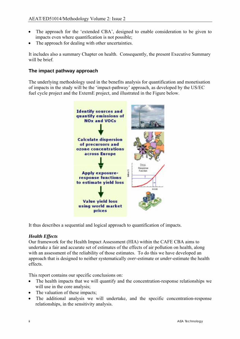
• The approach for dealing with other uncertainties. It includes also a summary Chapter on health. Consequently, the present Executive Summary will be brief. The impact pathway approach The underlying methodology used in the benefits analysis for quantification and monetisation of impacts in the study will be the �impact-pathway� approach, as developed by the US/EC fuel cycle project and the ExternE project, and illustrated in the Figure below.
It thus describes a sequential and logical approach to quantification of impacts. Health Effects Our framework for the Health Impact Assessment (HIA) within the CAFE CBA aims to undertake a fair and accurate set of estimates of the effects of air pollution on health, along with an assessment of the reliability of those estimates. To do this we have developed an approach that is designed to neither systematically over-estimate or under-estimate the health effects. This report contains our specific conclusions on: • The health impacts that we will quantify and the concentration-response relationships we
will use in the core analysis; • The valuation of these impacts; • The additional analysis we will undertake, and the specific concentration-response
relationships, in the sensitivity analysis.
AEAT/ED51014/Methodology Volume 2: Issue 2
AEA Technology iii
Our approach to evaluating impacts is presented below. The analysis will evaluate the impacts on health of air pollution, concentrating on the two main pollutants of concern � PM and ozone. The analysis has separated impacts into those considered in the main analysis (�core�), and additional impacts considered as part of the sensitivity analysis (�sensitivity�). Core functions are those for which evidence are best, sensitivity functions are those for which there is good evidence of effect, but a weakness at some point in the impact pathway. The sensitivity functions also include alternative analysis for certain impacts. Chronic mortality from PM amongst those aged over 30 • Following WHO guidance to RAINS, we will use the central estimate of a 6% increase in
mortality hazard rates per 10 µg/m3 PM2.5, implemented for anthropogenic PM, with no threshold.
• Consistent with WHO guidance, our own established practice, and a wider emerging consensus in favour of using life table methods, the analysis will express health impacts in terms of years of life lost from air pollution. The study team also recommends years of life lost as the most relevant metric for valuation. Empirical studies provide direct estimates of the value of a life year lost (VOLY), and there has been recent work deriving VOLY values (computationally) from the value of statistical life (VOSL) in the air pollution context.
• In addition, consistent with the recommendations of the peer review, the analysis will also include estimates of the number of deaths per year attributable to long-term exposure to ambient PM2.5. Estimates of attributable deaths have their own methodological problems. However, number of premature deaths appear easy to understand, and so are often made in HIAs of air pollution and health. The approach used here estimates attributuble deaths using a �static� approach (without life tables) where the annual death rate is multiplied by the PM2.5 risk factor. This method is approximate and is considered to over-estimate the true attributable fraction to some extent.
• Consequently mortality effects of long-term exposure to PM will be expressed both as years of life lost and as attributable cases of premature mortality and both are relevant for monetary valuation.
• We will not separately add in impacts of PM on mortality derived using the time-series studies. This is in order to avoid double counting with the cohort based analysis above. We will however estimate deaths using the WHO meta-analysis value of 0.6% change in earlier deaths, per 10 µg/m3 PM2.5, PM2.5 � 10, and PM10 for the purposes of illustration (for sensitivity analysis).
Infant mortality from PM The analysis of mortality effects from long-term exposure to PM only applies to adults. There is now substantial evidence that higher levels of air pollution is adversely associated with a wide range of measures of foetal and infant health, including mortality. The WHO is currently completing a comprehensive review of the effects of air pollution on children�s health. We also note that in quantifying the benefits to health of the US Clean Air Act, it has been recommended that infant mortality be included for quantification. • Infant mortality will be quantified in the CAFE CBA. • For quantification, we will use the cohort study by Woodruff et al. (1997), consistent with
the approach used in the US. Following Kaiser et al. (2004), we will implement in terms of attributable cases, rather than life-years, i.e. a different approach to that in adults above.
AEAT/ED51014/Methodology Volume 2: Issue 2
iv AEA Technology
Acute mortality from ozone in the general population • Following WHO guidance to RAINS, effects of daily ozone on (�acute�) mortality will be
quantified for the core analysis only at concentrations greater than 35ppb (maximum 8-hr mean). WHO recognised that estimating effects only above a cut-off point is a conservative approach to the estimation of the mortality effects of ozone, and consequently recommended a sensitivity analysis with no cut-off point (or equivalently, with cut-off point at zero) as an upper bound of impacts. Sensitivity analysis will therefore include quantification for concentrations greater than 0ppb.
• Following WHO, we will use a risk estimate of 0.3% increase in daily mortality per 10 µg/m3 O3 � this is the estimate from the WHO-sponsored meta-analysis of time series studies in Europe.
• Mortality impacts will be expressed initially in terms of numbers of cases. Note that the health impact here can best be characterised as a �deaths brought forward� attributed to ozone. This is to signify that people whose deaths are brought forward by higher air pollution almost certainly have serious pre-existing cardio-respiratory disease and so in at least some of these cases, the actual loss of life is likely to be small � the death might have occurred within the same year and, for some, may only be brought forward by a few days.
• The numbers of deaths will therefore be converted to life years lost. An estimate of six months was used in the ExternE project and the project team initially proposed to use this estimate for CAFE. The peer review team for this study considered that a larger value, on average, was warranted. A peer reviewed US evaluation of ozone and mortality has used an estimate of 12 months. On this basis we will assume that on average, each death brought forward involves a loss of life of 12 months. A range of estimates of average life years lost will be examined in sensitivity analyses, from 3 months to 3 years.
Valuation of mortality amongst adults and in the general population • Valuation of mortality linked to air pollution has been the subject of debate for a number
of years. This led to the commissioning of two research studies, one in the UK (here referred to as the �DEFRA study�) and the other for the European Commission, DG Research (the �NewExt study�). Both provide values in terms of the value of a statistical life (VSL) and, either directly or through computational analysis, the value of a life year (VOLY). Of the two studies, the results of NewExt will be used in CAFE, because they include samples from three European countries, whereas the DEFRA work was UK-specific. However, there was some consistency in the results of the two studies and this supports the methodologicical choices made in the CAFE benefit analysis.
• In terms of selecting values from either study, two issues are paramount. The first concerns whether we should use the VSL or VOLY for mortality valuation. Opinion is split on this issue. Some argue that the VOLY approach links more naturally to the quantified health impact. Others, however, argue that the VOLY concept lacks the strong empirical base developed by VSL estimates made over many years. The peer review team considered it appropriate to use both techniques and we will follow their recommendation to demonstrate sensitivity to this parameter. The second issue is whether it is more appropriate to use the median sample value from the underlying valuation studies (limiting the effect of high-end votes possibly made in protest), or the mean of the samples (remembering that the distribution of income in the population is highly skewed). Despite some initial preference for the median value, both the median and mean will be used following the advice of the peer reviewers, again to demonstrate sensitivity to this parameter.
• The estimates to be used, taken from NewExt and adjusted from 2003 to year 2000 values, are as follows:

AEAT/ED51014/Methodology Volume 2: Issue 2
AEA Technology v
o VOLY (median): �52,000 o VOLY (mean): �120,000 o VSL (median): �980,000 o VSL (mean): �2 million.
• It is noted that the median NewExt VSL of around �1 million is consistent with the value of statistical life used in other parts of the EC for cost-benefit analysis (e.g. for other environmental aspects and similar to other applications such as transport accidents).
• As some of the benefits in life years will occur in the future (potentially over a much longer time frame than for the CAFE scenario), we will consider the discounting of benefits, using a discount rate that is consistent with the other parts of the CAFE analysis (e.g. on costs) and, indeed, analysis for the European Commission more generally. For the core analysis this will be consistent with a social rate of time preference of 4%.
• Some additional values are included for sensitivity analysis, based on the peer review comments. However, we have not followed the peer review advice to adopt separate values for individual countries in Europe. This is due to the fact that it was considered technically impossible and politically inappropriate to try to derive a VSL (and computationally a VOLY) for each EU Member State.
Valuation of infant mortality • Parents are more willing to pay to reduce their children�s health risks than their own. The
estimated marginal rate of substitution (MRS) is generally greater than one, and is typically about 2. However, there are several methodological difficulties with valuation of childhood mortality that remain unresolved.
• This value is broadly consistent with a life-years approach that attributes a full life expectancy of somewhat less than 80 years to each infant death, and about half as many life-years on average to healthy adults. It is not known whether the infants whose death occurs prematurely from air pollution are a particularly vulnerable subset, with lower than average life expectancy regardless of air pollution.
• There is an EC-funded project that has the remit to undertake new empirical work on valuation of children�s mortality risks in Europe, but this will not be available within the study time-scale.
• At this stage our recommendation is to use values for the adult-child MRS of 1, 1.5 and 2 with regard to the adult VSLs of �0.98 million and �2 million. This leads to a range of �0.98 million to �4 million, with central estimates of �1.5 million and �3 million.
• These values are broadly consistent with, but generally more conservative than, a value based on VOLY of �52,000 which would be equivalent to around �4m per mortality.
• We will also undertake a sensitivity analysis to assess mortality in children/young adults (i.e. the gap between that covered by the cohort analysis, and infant mortality analysis).
Morbidity from PM and ozone • The health analysis will also assess morbidity impacts from PM and ozone. For PM, these
will include the effects of acute exposures (from observation of response to day-to-day variations in ambient PM) as well as of long-term (chronic) exposures. It may be that there are specific adverse effects of long-term exposure to ozone also, but current evidence points to quantification of acute effects only.
• Ambient PM is associated with effects on the cardiovascular system as well as the respiratory system; effects of ozone on morbidity have been shown clearly for respiratory effects only.
AEAT/ED51014/Methodology Volume 2: Issue 2
vi AEA Technology
• As for mortality, we will quantify effects of anthropogenic PM, without threshold; and effects of ozone above daily maximum 8-hr mean of 35 ppb for the core analysis, and with no cut-off point for sensitivity analysis. Our approach is outlined below.
• Emergency hospital admissions: We will quantify effects of daily variations in PM and ozone on (emergency) hospital admissions for respiratory diseases and, for PM only, on admissions for cardiac disease. In order to link with available data on background rates, we will use all-ages C-R functions and background rates from the EU-funded APHEIS project, whose 3rd report (APHEIS-3) has recently been published. Concentration-response (C-R) functions are given by age-group in the WHO-supported meta-analysis of relevant studies in Europe. To a limited extent we will use these in sensitivity analyses.
• Consultations with primary care physicians: We will use impact functions for three pathways, but use them for sensitivity analysis only, because the functions are derived from studies in one city only (London) and may not be representative across Europe:
o PM and consultations for asthma o PM and consultations for upper respiratory symptoms (excluding allergic
rhinitis) o Ozone and consultations for allergic rhinitis
• Various HIA studies have shown that restricted activity days (RADs) and minor restricted activity days (MRADs), though rarely studied epidemiologically, can make a major contribution to the benefits of reducing air pollution.
o Using US studies, we have quantified an effect of PM on RADs, for core analyses. These RADs include relatively severe effects (for example when a person is restricted to bed) as well as minorRADs, and so for subsequent valuation, we have attributed the relative proportion of RAD:MRAD.
o For sensitivity analyses we have also quantified an effect of PM on work loss days (WLDs) and on MRADs. These two are additive to one another but not to RADs, with which they overlap.
o We have also quantified an effect of ozone on MRADs. o Sensitivity analyses will explore the effect of extrapolating from adults of
working age, to all adults. • The WHO meta-analysis also provides C-R functions for cough and respiratory
medication usage in individuals with underlying respiratory disease. With regard to respiratory medication, we have used the WHO meta-analysis and the papers cited there to define impact functions both for PM and for ozone, both for adults and for children with asthma. Several of these functions are not statistically significant, but are included for completeness because air pollution is widely recognized as exacerbating asthma.
• We have developed substantially the evaluation of how PM and ozone affect respiratory symptoms. This has led to the following set of impact functions:
o For PM: lower respiratory symptoms (LRS), including cough, among adults with chronic respiratory symptoms; and LRS (including cough) among children in the general population � both for core analyses
o For O3: respiratory symptoms among adults in the general population, and both cough, and LRS excluding cough, among children in the general population.
• There are some additional endpoints for which there is evidence of chronic exposures. The most important of these are likely to be effects of PM on chronic bronchitis, which we will quantify in the core analysis using C-R functions and background rates from the US AHSMOG study. The main omission is that we have been unable to find any suitable studies that would permit quantification of an effect of long-term exposure to PM on the development or progression of chronic cardiovascular disease.

AEAT/ED51014/Methodology Volume 2: Issue 2
AEA Technology vii
Valuation of morbidity impacts • For valuation, where data is available, we will use an empirical study covering five
countries across Europe (Day et al, 1999; Navrud et al, 2001; Ready et al. 2004). Recommended values for the effects that will be quantified are shown in Table (i) below.
• A number of US valuation studies have assessed chronic morbidity effects of PM, and we will use a central estimate of �190,000 per case, based on their findings.
Table (i) Summary of health valuation data for the CAFE CBA
Mortality Based on median values Based on mean values Infant mortality � 1,500,000/death � 4,000,000/death Value of statistical life � 980,000/death � 2,000,000/death Value of a life year � 52,000/year � 120,000/year
Morbidity Low Central High Chronic bronchitis � 120,000/case � 190,000/case � 250,000/case Respiratory, cardiac hospital admission
� 2,000/admission
Consultations with primary care physicians
� 53/consultation
Restricted activity day (day when person needs to stay in bed)
� 130/day
Restricted activity day (adjusted) � 83/day Minor restricted activity day � 38/day Use of respiratory medication � 1/day Symptom days � 38/day Additional sensitivity analysis Subject to necessary pollution data being available, we will undertake a number of additional sensitivities: • The first and most important is to discuss qualitatively, and if possible examine
quantitatively in sensitivity analyses, the potential effects of different toxicities for the components of the PM mixture, i.e. primary PM2.5, sulphates and nitrates. We recognise that any attempt at quantification will be speculative. The Health Effects Task Force of WHO considered this issue in 2003, and again in the CAFE follow-up questions. The latter noted that:
o Toxicological studies have highlighted that primary, combustion-derived particles have a high toxic potency; and that
o Several other components of the PM mix � including sulphates and nitrates � are lower in toxic potency;
• Unfortunately there is a lack of any established risk estimates for the different components. We agree with the WHO (2004) evaluation that it is currently not possible to precisely quantify the contributions from different sources and different PM components to health effects. However, we believe there is value in exploring this as a sensitivity analysis, for example to differentiate between policies that reduce primary rather than secondary particles from combustion.
• Additional sensitivity analysis for other pollutants, notably SO2 and NO2 as gases, will be considered subject to pollution data availability. At present we have not developed C-R functions for these pollutants.
AEAT/ED51014/Methodology Volume 2: Issue 2
viii AEA Technology
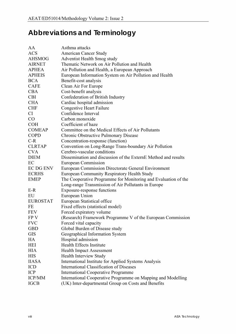
Abbreviations and Terminology AA Asthma attacks ACS American Cancer Study AHSMOG Adventist Health Smog study AIRNET Thematic Network on Air Pollution and Health APHEA Air Pollution and Health, a European Approach APHEIS European Information System on Air Pollution and Health BCA Benefit-cost analysis CAFE Clean Air For Europe CBA Cost-benefit analysis CBI Confederation of British Industry CHA Cardiac hospital admission CHF Congestive Heart Failure CI Confidence Interval CO Carbon monoxide COH Coefficient of haze COMEAP Committee on the Medical Effects of Air Pollutants COPD Chronic Obstructive Pulmonary Disease C-R Concentration-response (function) CLRTAP Convention on Long-Range Trans-boundary Air Pollution CVA Cerebro-vascular conditions DIEM Dissemination and discussion of the ExternE Method and results EC European Commission EC DG ENV European Commission Directorate General Environment ECRHS European Community Respiratory Health Study EMEP The Cooperative Programme for Monitoring and Evaluation of the
Long-range Transmission of Air Pollutants in Europe E-R Exposure-response functions EU European Union EUROSTAT European Statistical office FE Fixed effects (statistical model) FEV Forced expiratory volume FP V (Research) Framework Programme V of the European Commission FVC Forced vital capacity GBD Global Burden of Disease study GIS Geographical Information System HA Hospital admission HEI Health Effects Institute HIA Health Impact Assessment HIS Health Interview Study IIASA International Institute for Applied Systems Analysis ICD International Classification of Diseases ICP International Cooperative Programme ICP/MM International Cooperative Programme on Mapping and Modelling IGCB (UK) Inter-departmental Group on Costs and Benefits
AEAT/ED51014/Methodology Volume 2: Issue 2
AEA Technology ix
IHD Ischaemic Heart Disease IOM Institute of Occupational Medicine ISAAC International Study of Asthma and Allergies in Children LFS Labour Force Survey LRS Lower respiratory symptom LRTAP Convention on Long Range Transboundary Air Pollution LY or LYL Life years (lost) MFR Maximum feasible reduction scenario MRAD Minor restricted activity day MRS Marginal rate of substitution NCHS National Centre for Health Statistics NEBEI Network of experts on benefit and economic instruments NECD National Emission Ceilings Directive NEEDS New Energy Externalities Developments for Sustainability NMMAPS National Mortality, Morbidity, and Air Pollution Study NO Nitrogen monoxide NO2 Nitrogen dioxide NO3
- Nitrate NOx Oxides of nitrogen NPHS National Population Health Survey O3 Ozone ORNL Oak Ridge National Laboratory PEACE Pollution Effects on Asthmatic Children in Europe study PM10 Fine particles less than 10 µm in diameter PM2.5 Fine particles less than 2.5 µm in diameter QWB Quality of well being RAD Restricted Activity Day RAINS Regional Air Pollution Information and Simulation RE Random effects (statistical model) REF Reference scenario RFF Resources For the Future RHA Respiratory Hospital Admission RR Relative Risk RRAD Respiratory restricted activity day SE Standard error SO2 Sulphur dioxide SO4
-- Sulphate SOMO 0 Sum of ozone (daily 8-hr max) means over 0 ppb (ppb.hours) SOMO 35 Sum of ozone (daily 8-hr max) means over 35 ppb (ppb.hours) TSP Total Suspended Particulates UNECE United Nations Economic Commission for Europe URD Upper respiratory disease USEPA United States Environmental Protection Agency VLYL Value of a life year lost VOCs Volatile organic compounds VOLY Value of life year

AEAT/ED51014/Methodology Volume 2: Issue 2
x AEA Technology
VOSL Value of statistical life VSL Value of statistical life WHO World Health Organization WHO-TFH WHO-Task Force on Health WLD Work Loss Day WTA Willingness to accept WTP Willingness to pay YOLL Years of life lost MATHEMATICAL NOTATION
The following prefixes and suffixes are used in this work; Ex, E-x as a suffix to a number, denotes that the number in question should be multiplied by
10 to the power x or -x. Hence 6.4E-3 is equal to 0.0064. The following prefixes to units are also used; n = nano = 10-9 µ or u = micro = 10-6 m = milli = 10-3 k = kilo = 103 = thousands M = mega = 106 = millions G = giga = 109 = billions This system is standard notation in the sciences. Note that m and M are not equivalent (by a factor of 109) and hence should not be interchanged.

AEAT/ED51014/Methodology Volume 2: Issue 2
AEA Technology xi
Contents
1. BACKGROUND MATERIAL ON HEALTH. GENERAL PRINCIPLES AND UNDERLYING EVIDENCE........................................................................................ 1
1.1. INTRODUCTION............................................................................................................ 1 1.2. METHODOLOGICAL FRAMEWORK. ............................................................................... 1
1.2.1 What is the purpose of the work and what are we trying to achieve?................ 1 1.2.2 The review process during development of this methodology............................ 2 1.2.3 What sources will we draw on? How much new and fundamental work will we carry out on assessing the epidemiological and other health literature?.......................... 2 1.2.4 What issues will we focus on? ............................................................................ 3
1.3. KEY ISSUES IN ASSESSING HEALTH IMPACTS OF AMBIENT AIR POLLUTION................... 3 1.3.1 Evaluating the effects of mixtures/ allocation of damages to specific pollutants – general principles............................................................................................................ 3 1.3.2 Thresholds: will the main implementations assume a threshold or not?........... 5 1.3.3 Quantification and valuation of mortality impacts ............................................ 7 1.3.4 Quantification of morbidity effects..................................................................... 7
1.4. POPULATION (STOCK AT RISK) DATA........................................................................... 8 1.5. CONCENTRATION-RESPONSE (C-R) FUNCTIONS .......................................................... 9
1.5.1 C-R functions used in ExternE, and the need to update them............................ 9 1.5.2 Using international or local C-R functions; transferability of C-R functions . 12
1.6. QUANTIFYING THE EFFECTS OF MIXTURES: THE ROLE OF SPECIFIC POLLUTANTS ....... 12 1.6.1 Attributing effects to particles or to the gases.................................................. 13 1.6.2 Attributing effects of PM to specific types or fractions of particles................. 13
1.7. PARTICULAR ISSUES FOR ASSESSMENT OF MORTALITY.............................................. 15 1.7.1 Different kinds of studies identify the mortality effects of acute and chronic exposure 15 1.7.2 Cohort and time series studies provide different kind of information about mortality; what metric should be used? ........................................................................... 15 1.7.3 Which type of evidence has priority? Can cohort and time series results be added? 16
2. SPECIFIC DECISIONS ON METHODOLOGY � GENERAL ISSUES................ 18 2.1. INTRODUCTION.......................................................................................................... 18
2.1.1 Status ................................................................................................................ 18 2.1.2 Structure of this health report .......................................................................... 18
2.2. FRAMEWORK ISSUES ................................................................................................. 19 2.2.1 Note on terminology: Acute and chronic exposure and effects........................ 19 2.2.2 General principles of HIA ................................................................................ 19 2.2.3 Existing reviews................................................................................................ 20 2.2.4 HIA work within RAINS and for the benefits analysis of CAFE CBA.............. 22 2.2.5 Mixtures, attributing effects to specific pollutants, including which particles 25 2.2.6 Deriving impact functions from use in morbidity evaluations ......................... 28
3. QUANTIFICATION OF MORTALITY .................................................................... 30 3.1. INTRODUCTION.......................................................................................................... 30 3.2. MORTALITY EFFECTS OF LONG-TERM (CHRONIC) EXPOSURE TO AMBIENT PARTICLES30
3.2.1 Choice of effect estimate in terms of % change per unit pollutant .................. 30
AEAT/ED51014/Methodology Volume 2: Issue 2
xii AEA Technology
3.2.2 Using life tables to estimate the associated mortality impacts in the target population – methodological issues in estimating results in terms of life-years ............. 33 3.2.3 Using life tables to estimate the associated mortality impacts in the target population – illustrative example: context, methods and results for a 1-yr pulse change 37 3.2.4 A comparison of the CAFE approach with that used by the WHO Global Burden of Disease Project................................................................................................ 38 3.2.5 Moving towards valuation................................................................................ 39 3.2.6 Should (some of) the effects of PM as estimated from time series studies be added to the PM effects as estimated from cohort studies? ............................................. 42
3.3. EFFECTS ON MORTALITY OF SHORT-TERM EXPOSURE (ACUTE EXPOSURE, DAILY VARIATIONS) TO OZONE ........................................................................................................ 43
3.3.1 Which pollutants?............................................................................................. 43 3.3.2 Estimating impacts of ozone reduction in terms of ‘deaths postponed’ (attributable cases avoided) ............................................................................................. 43 3.3.3 Linkage with monetary valuation..................................................................... 44 3.3.4 Inferring life years saved.................................................................................. 45
4. VALUATION OF MORTALITY................................................................................ 47 4.1. INTRODUCTION.......................................................................................................... 47 4.2. METRICS FOR MORTALITY VALUATION...................................................................... 47
4.2.1 Value of statistical life...................................................................................... 47 4.2.2 Value of a life year ........................................................................................... 48 4.2.3 Measurement of the cost per life saved (CPLS)/cost per life year saved (CPLYS) 49 4.2.4 Conclusions of the Commission’s Working Group (EC, 2000) ....................... 50
4.3. NEW EMPIRICAL EVIDENCE........................................................................................ 51 4.3.1 The NewExt study ............................................................................................. 51 4.3.2 The DEFRA study............................................................................................. 54
4.4. SUMMARYOF VALUES TO BE USED IN THECAFE CBA .............................................. 55
5. QUANTIFICATION OF MORTALITY IN INFANTS AND YOUNG CHILDREN ........................................................................................................................... 59
5.1. EFFECTS OF CHRONIC EXPOSURE ON INFANT MORTALITY.......................................... 59 5.1.1 Available research............................................................................................ 59 5.1.2 Use of cohort or of time series studies ............................................................. 60 5.1.3 Frailty; study deaths (attributable cases) or life-years.................................... 60 5.1.4 Cause-specific or all-cause mortality .............................................................. 61 5.1.5 Which pollutant? .............................................................................................. 61 5.1.6 Transferability; functions for an implementation in Europe ........................... 61 5.1.7 Recommendation .............................................................................................. 61
5.2. EFFECTS OF ACUTE EXPOSURE IN CHILDREN UNDER FIVE YEARS; AND, MORE GENERALLY, MORTALITY EFFECTS (CHRONIC AND ACUTE EXPOSURE) IN PEOPLE UNDER 30 YEARS OF AGE ....................................................................................................................... 62
6. VALUATION OF MORTALITY IN INFANTS AND YOUNG CHILDREN........ 64 6.1. INTRODUCTION.......................................................................................................... 64 6.2. METHODOLOGICAL ISSUES ........................................................................................ 64 6.3. EMPIRICAL ISSUES ..................................................................................................... 65
7. QUANTIFICATION OF MORBIDITY ..................................................................... 67

AEAT/ED51014/Methodology Volume 2: Issue 2
AEA Technology xiii
7.1. MORBIDITY � METHODOLOGY; LIMITED USE OF IMPACT FUNCTIONS ....................... 67 7.1.1 Basic approach................................................................................................. 67 7.1.2 Impact functions ............................................................................................... 67
8. MORBIDITY FROM CHRONIC EXPOSURE: PARTICULATE MATTER....... 69 8.1. THE EVIDENCE........................................................................................................... 69 8.2. PRIORITIES FOR QUANTIFICATION.............................................................................. 69 8.3. NEW CASES OF CHRONIC BRONCHITIS, IN ADULTS ..................................................... 69
8.3.1 Choice of endpoint – new cases of ‘chronic bronchitis’ .................................. 70 8.3.2 Background rate............................................................................................... 70 8.3.3 C-R function in metric of PM10, from Abbey et al. (1995a) ............................. 71 8.3.4 Impact function in metric of PM10, from Abbey et al. (1995a)......................... 72 8.3.5 C-R function in metric of PM2.5, from Abbey et al. (1995b)............................. 72 8.3.6 Impact function................................................................................................. 72 8.3.7 Preferred impact function ................................................................................ 73 8.3.8 Comments on reliability ................................................................................... 73
9. MORBIDITY FROM CHRONIC EXPOSURE: OZONE........................................ 74 9.1. THE EVIDENCE........................................................................................................... 74 9.2. INCIDENCE OF DOCTOR-DIAGNOSED ASTHMA IN ADULT MEN .................................... 74
10. MORBIDITY FROM ACUTE EXPOSURES: PARTICULATE MATTER AND OZONE......................................................................................................................... 76
10.1. HOSPITAL ADMISSIONS.......................................................................................... 76 10.1.1 Introductory remarks........................................................................................ 76 10.1.2 Cardiovascular hospital admissions – in practice, cardiac hospital admissions (CHA, ICD 390-429) ........................................................................................................ 77 10.1.3 Respiratory hospital admissions (RHA; ICD 460-519) ................................... 78 10.1.4 Consultations with primary care physicians (general practitioners) .............. 81
10.2. AIR POLLUTION AND RESTRICTIONS ON USUAL ACTIVITIES.................................... 85 10.2.1 Definitions; choice of study – the US Health Interview Study (HIS) ............... 85 10.2.2 Restricted activity days (RADs) and PM2.5 (Ostro, 1987)................................ 86 10.2.3 Work loss days (WLDs) .................................................................................... 88 10.2.4 Minor restricted activity days (MRADs): Ostro and Rothschild, 1989........... 89
10.3. EFFECTS OF PM AND OZONE ON MEDICATION USE BY PEOPLE WITH ASTHMA........ 91 10.3.1 Brief remarks on medication use by people with asthma................................. 91 10.3.2 Medication use by children with asthma.......................................................... 92 10.3.3 Medication use by adults with asthma ............................................................. 97
10.4. PM, OZONE, AND RESPIRATORY SYMPTOMS........................................................ 100 10.4.1 Introductory remarks about studies of respiratory symptoms ....................... 100 10.4.2 PM and acute respiratory symptoms in children ........................................... 100 10.4.3 Ozone and acute respiratory symptoms in children....................................... 104 10.4.4 PM and respiratory symptoms in adults ........................................................ 106 10.4.5 Ozone and respiratory symptoms in adults .................................................... 110 10.4.6 Final comments on respiratory symptoms and medication usage in adults and children 112
10.5. PM, OZONE AND MINOR CHANGES IN CARDIO RESPIRATORY FUNCTION .............. 113 10.6. CONCLUSION: HEALTH IMPACTS (MORBIDITY) TO BE QUANTIFIED...................... 114
11. VALUATION OF MORBIDITY............................................................................... 115 11.1. INTRODUCTION.................................................................................................... 115
AEAT/ED51014/Methodology Volume 2: Issue 2
xiv AEA Technology
11.2. COST ESTIMATES FOR SPECIFIC ENDPOINTS ......................................................... 116 11.2.1 Component (i): Health care resource costs ................................................... 116 11.2.2 Component (ii): The costs of absenteeism...................................................... 116 11.2.3 Hospital admissions ....................................................................................... 117 11.2.4 Emergency room visits for respiratory illness ............................................... 118 11.2.5 GP visits: Asthma & lower respiratory symptoms ......................................... 118 11.2.6 Restricted activity days (RAD) ....................................................................... 118 11.2.7 Respiratory symptoms in people with asthma: Adults and children .............. 119 11.2.8 Respiratory medication use by children and adults ....................................... 119 11.2.9 Chronic bronchitis (new cases)...................................................................... 119 11.2.10 Other end-points......................................................................................... 121
11.3. SUMMARY OF HEALTH ENDPOINTS ...................................................................... 121
12. REFERENCES............................................................................................................ 122
AEAT/ED51014/Methodology Volume 2: Issue 2
AEA Technology 1
1. Background Material on Health. General Principles and Underlying Evidence
1.1. Introduction There are many significant issues to be considered in the assessment of the health damages, particularly as health damages and the reliability with which they have been assessed have dominated past work on air pollution benefits assessment. The present Chapter has the objective of highlighting key issues to be addressed in CAFE CBA and outlining how they have been tackled. In particular, it sets out a framework of general principles which guided the development of the later Chapters.
1.2. Methodological framework.
1.2.1 What is the purpose of the work and what are we trying to achieve? What we are trying to achieve within the CAFE CBA is a fair and accurate set of estimates of the effects of air pollution on health, along with a fair and accurate assessment of the reliability of those estimates. By �fair and accurate� we mean a methodology which neither systematically over-estimates or under-estimates the health effects. This means that, in the face of unavoidable uncertainties in estimating health effects:
a. We will not assume a worst-case position, i.e. that the true effects of air pollution are the most severe that can be supported by evidence. Giving �the benefit of the doubt� to that evidence which supports strongest effects of air pollution on health, i.e. building the precautionary principle directly into the HIA itself, gives rise to a methodology that systematically over-estimates health effects. It is better that the precautionary principle should be applied when decisions are being made about various policies, using the results of the HIA/ CBA, and other inputs.
b. We will not restrict our assessment to those aspects of a quantification on which there is agreement that amounts to a consensus. If we think that the assessment can be improved substantially by including aspects on which there is not yet a consensus, we will if practicable do so. Not to do so would mean we were using a methodology that systematically under-estimates health effects. However, in our uncertainty assessments, and in reporting results, we will distinguish aspects and assumptions on which there is widespread agreement form those on which there isn�t.
To re-iterate: we think that the CAFE CBA will be a better support to policy-making, and that its role in policy making will be more transparent, if we aim for a fair and accurate assessment, rather than one which systematically over-estimates or under-estimates effects, however plausible the reasons for over- or under-estimation. The CAFE CBA will evaluate a range of different scenarios, with different mixtures of pollutants. We will aim to give a fair and accurate assessment of the health effects of each scenario, even if in doing so there is some inconsistency between scenarios in the effects we attribute to individual pollutants. This is discussed further under mixtures, below.
AEAT/ED51014/Methodology Volume 2: Issue 2
2 AEA Technology
The CAFE CBA will mainly evaluate the impacts on health of air pollution mixtures insofar as they can be characterised by the �classical� air pollutants � particulate matter (PM) and the gases: ozone, SO2, NO2, CO. It will not seek to evaluate directly the effects on health of heavy metals such as nickel, arsenic, and lead, or other pollutants such as PAHs.
1.2.2 The review process during development of this methodology Over the past few months, we have discussed our approach at a number of important meetings:
• On April 28th, at the joint meeting in Bonn of two relevant Working Groups of AIRNET: Health Impact Assessment, and Science-Policy Interface;
• On April 30th, at a special stakeholders workshop in Brussels; and • On May 6th and 7th, at the meeting in Bonn of the WHO Task Force on Long-Range
Trans-Boundary Air Pollution. • On 16th July 2004, at a workshop to discuss the third draft of the methodology report. • In October 2004, at a joint EC-CLRTAP workshop in Gothenburg
In addition to the comments of stakeholders, the methodology has been subject to independent peer review. This reported in October 2004. Overall, the methodology adopted here for the health impact assessment has subject to a far greater level of scrutiny and debate than that carried out for the previous CBAs under the Air Quality Framework Directive and the NEC Directive.
1.2.3 What sources will we draw on? How much new and fundamental work will we carry out on assessing the epidemiological and other health literature?
We have drawn on work being done for a number of other projects. Specifically, for HIA we have used the following several �pillars� to construct and refine the methodology.
a. The ExternE programme and projects of the EU, including ongoing Framework Programme (FP) V projects such as DIEM and NewExt, and (where timescales and concordance of issues permit) new FP projects such as NEEDS. In our view, many of the basic judgments and methodological innovations of ExternE remain very relevant, but the specific concentration-response (C-R) functions used needed to be re-considered and updated.
b. The work of the World Health Organisation whose experts have answered a wide range of questions about air pollution and health, specifically for the benefit of CAFE. These WHO answers have drawn on the experience and judgment of key researchers and policy makers both in Europe and in North America and as such, they provide the best available distillation of the current understanding of the air pollution research community on a wide range of difficult issues.
c. The HIA work of other established teams. Within Europe, general methodological issues are currently being assessed within the HIA Working Group of the AIRNET network. Here, the work of the APHEIS team is especially important, because it draws on the experience of APHEA researchers, and also of the HIA/ CBA team led by Nino Künzli. Also, there is currently a major HIA/ CBA project being carried out by the US EPA, as one of its evaluations of the costs and benefits of the US Clean Air Act.
AEAT/ED51014/Methodology Volume 2: Issue 2
AEA Technology 3
d. Finally, as outlined above, we have sought opinions and comments from stakeholders on our ideas as they evolve.
It was initially intended that we would do very little new evaluations of the literature for CAFE CBA specifically. Rather, the CAFE CBA methodology for health, as for other impacts, would be constructed as the best available hybrid from many other established sources. However, during the course of the work the views of the team have changed on this issue, and a substantial amount of new review has been conducted. This has been necessary in order to refine methods with respect to functions and background rates in particular, and to expand the range of endpoints considered in the development of the methodology.
1.2.4 What issues will we focus on? Assessment of the effects of air pollution on health is an area of the interface of science and policy where quantitative HIA/ CBA methods are most strongly developed and used. This would not have been possible without the great growth in research on air pollution and health during the past 15 years or so. That same time-period has also seen substantial development of HIA/ CBA methods in the context of air pollution and health. Nevertheless, there is a multitude of issues where there are gaps in knowledge and/or uncertainties and lack of consensus on interpreting the knowledge available. It is neither practicable nor necessary for CAFE CBA to consult on and form a fully informed opinion on all these issues. Many issues and uncertainties, while interesting and important in their own right, have little bearing on the final results of a HIA/ CBA. In the present study we focus most attention on those issues which are most likely to have an important bearing on the final answers of the evaluation. We identify those issues based on our experience, on the experience and practice of others, and on the results of preliminary modelling. We also, necessarily, pay attention to issues raised by stakeholders, whether or not they have an important bearing on final results. However our prioritisation of issues has been influenced throughout by what is sometimes called the DIM philosophy � Does It Matter?
1.3. Key issues in assessing health impacts of ambient air pollution
1.3.1 Evaluating the effects of mixtures/ allocation of damages to specific pollutants – general principles
The issue The underlying issue here is simple but not easy. Briefly, the epidemiological studies which give rise to the C-R functions used in HIA are based on studies of air pollution mixtures, generally in urban areas. The health effects of the mixture as a whole are examined and associations with specific pollutants are examined. Often the applications of HIA are, however, to specific pollutants or to other mixtures. Application to mixtures is done by
• Disaggregating the mixture into its component parts � in CAFE CBA, characterising it in terms of the classical pollutants;
• Estimating effects associated with each component; and then • Re-aggregating effects, to give an estimate of the benefits of changes in the mixture.
AEAT/ED51014/Methodology Volume 2: Issue 2
4 AEA Technology
Assessing the causality of specific pollutants (specific components of a mixture) and/or of specific epidemiological associations It is difficult to interpret the associations found, from the viewpoint of causality, because it is well-known that association does not necessarily imply causality. (By causality here we mean that changes in a pollutant will lead to changes in risk to health, and so ultimately to changes in health impacts. Specifically, we mean that reductions in the named pollutant will lead to benefits to health.) The likelihood that an association is causal is enhanced by consistency of findings across different times and locations, and especially across different kinds of air pollution mixtures. Experimental toxicological studies (controlled human studies; animal studies; cell studies) provide important information on pollutant-specific effects and possible mechanisms of action. Eventually, however, judgment is required, in the face of uncertainty, on the extent that associations found are causal in the named pollutant, or whether that pollutant is acting as a �tracer� or surrogate for other aspects of the mixture, or whether that particular association from that study is a chance result (if even statistically significant). Constructing a ‘model’ of the effects of a mixture We have found it helpful to think of the process of HIA/ CBA as constructing a model (note, this is not a computational model, but rather an implementation framework) for the health effects of a mixture. By this we mean constructing a simplified but nonetheless useful schematic representation of a more complex reality. In HIA/ CBA work on air pollution, a model is the totality of impact pathways quantified, together with the rules for aggregating them. An advantage of adopting this viewpoint is that it helps avoid the contentious issue of whether the impact assessment (the model) is �true� or �false�. In general, models are approximations to the complex reality they seek to represent, and as such, a safe working assumption is that they are always false, in the sense of being less than perfect, and open to improvement. They can, however, be better or worse; and thinking of the process as one of constructing a practical model can help structure discussion about important issues such as whether:
i. the results of the approach are fair and accurate; ii. suggested changes will improve its fairness and accuracy;
iii. suggested changes will make any important difference to results. In assessing impacts, can we avoid missing some effects? Can we avoid double-counting others? We will follow the general principles that we will aim to:
i. attribute effects that are causal in the mixture being evaluated; ii. attribute all effects; and
iii. attribute effects once only (i.e. avoid attributing the �same� health effect to different components of the mixture, and adding the resulting impacts).
Of these principles, the 3rd (avoiding double-counting) has received the most attention. For example, separating out the roles of SO2, NO2 and PM10 is particularly problematic, given that they vary together in most locations and studies. However, there is also information in differences between locations, for example in whether or not the apparent effects of PM are different when NO2 (or SO2) concentrations are high rather than low. A �hierarchy� for quantification is defined below.
AEAT/ED51014/Methodology Volume 2: Issue 2
AEA Technology 5
However, the 2nd issue is important also. It refers not only to specific impact pathways that are relevant but not quantifiable � though these can be noted in the extended CBA of the study. It includes also the extent to which health effects may be caused by aspects of the general air pollution mixture. For example, the number of very small particles is not measured routinely and in general there are not usable C-R functions expressed in terms of particle number. However, there are grounds for believing that particle number is one influential driver of the health effects of a mixture overall; and insofar as this is relevant, the effect can be captured indirectly only, via particle mass (not necessarily well correlated with number) and/or other surrogate or tracer pollutants, e.g. NO2. The lack of C-R functions in the relevant component can lead to under-estimation of effects, just as careless addition of impacts across pollutants can lead to double-counting. How important is this issue? The importance of the issue varies according to the applications HIA.
a. The least controversial is where the purpose of the quantification is to estimate the overall effect of air pollution on the exposed population. It does not matter much if the identified pollutants are really causal or are tracers of the overall mixture, provided that:
i. the mixture being evaluated is �similar enough� to those studied epidemiologically; and
ii. care is taken to ensure that health effects attributable to the mixture are neither missed nor double-counted.
In CAFE CBA, this circumstance arises principally in considering the baseline scenario, and assessing the health effects associated with it.
b. The issue becomes more important when assessing scenarios, because the mixtures to be evaluated may differ substantially from the �usual� mixtures of ambient air pollution in cites. (Here, the �mixture to be evaluated� may be a single pollutant; which of course does differ from the general urban mixture.) This will be the most frequent situation in CAFE CBA. The 1st step is to understand the target mixture as fully as possible, in its similarities and differences to what has been studied epidemiologically.
1.3.2 Thresholds: will the main implementations assume a threshold or not?
The issue here is whether or not, for the main air pollutants to be considered here, there exist thresholds at the population level; and specifically, whether the CAFE HIA/ CBA should be implemented assuming no threshold, or some threshold (and if so, at what level), or both. Working definition of ‘threshold at the population level’ It will help if we can clarify terms. By �threshold at the population level� we mean a concentration of the pollutant such that, at concentrations below that threshold, there is no increase in risk of adverse health effects in any of the exposed population-at risk. Note that in epidemiological studies, and in HIA, the relevant concentrations are not based on personal exposure monitoring of individuals. Rather, they are concentrations as measured at ambient fixed-point monitors, and referring either to daily concentrations (usually 24-hour daily averages) or to annual averages. �Threshold at the individual level� can be defined
AEAT/ED51014/Methodology Volume 2: Issue 2
6 AEA Technology
analogously, except that here, it is assumed (usually implicitly rather than explicitly) that the concentrations refer to measurements near the breathing zone of the individual. HIA, like epidemiology, is concerned with threshold at the population level, because it is applied to large and diverse populations of people, and uses concentration data as measured at (or modelled in relation to) fixed-point monitors. Does epidemiology support the existence of threshold at the population level? In general, epidemiological studies of the pollutants of interest have not supported the existence of thresholds at the population level. As discussed further below, both the nature and the strength of evidence vary by pollutant and indeed by specific health endpoint. In general we note that proposals for a population threshold for the main pollutants to be considered here have been contradicted by the accumulating evidence of studies. This is not surprising, given that there can be substantial variations in:
i. the susceptibility of individuals (or, the distribution of individual-level thresholds) in a large population of diverse ages and pre-existing health; and
ii. the relationship between daily (or annual average) personal exposure from ambient sources to the concentrations measured at nearest fixed-point monitors.
With both of these sources of variation acting concurrently, it is plausible that at any level of ambient fixed-point concentration, some (possibly small) proportion of the population-at-risk will nevertheless experience some personal exposures that contribute something to an increase in risk. We adopt a ‘no threshold’ assumption as the primary basis for quantification within CAFE This is not the same as saying that epidemiology has �proved� that there is no threshold at the population level. This cannot be proven � a judgment or assumption of �no threshold� always requires some extrapolation of the epidemiological evidence. It does, however, point to a �no threshold� interpretation of the epidemiological evidence, and so to a �no threshold� assumption in HIA implementation, as the way forward that is most consistent with current evidence and understanding. Our principal implementations will therefore take the assumption of �no threshold�. This position is consistent with the approach adopted in other major HIA exercises � ExternE, Künzli and colleagues, US EPA etc. However, we will also be consistent with the suggested approach for ozone used elsewhere in RAINS, and include a �cut-off� for implementation. This is discussed later. Anthropogenic sources and natural backgrounds The case is sometimes made that there are natural backgrounds of ozone (and of other pollutants also) and that either:
i. There are no adverse health effects associated with concentrations below these backgrounds, because they are �natural�; or that
ii. Any associated adverse health effects should not be quantified, because it is impossible to reduce pollution to below these levels.
AEAT/ED51014/Methodology Volume 2: Issue 2
AEA Technology 7
In practice this makes no difference to the quantification of effects to be carried out in CAFE, as this is typically done in an incremental fashion. For cost-benefit analysis the total impact is of little relevance, as it is the incremental change in costs and benefits that matters, not absolute values.
1.3.3 Quantification and valuation of mortality impacts It is now widely recognised that the effects on mortality of chronic (long-term) exposure to particles can and should be quantified. Also, that in HIA work that includes the effects of particles, these effects are the dominant ones in the assessment as a whole. In CAFE CBA these effects on mortality are to be quantified using the GIS tool, using methods that have been explored at IIASA and elsewhere (e.g. Hurley et al, 2000). Although the RAINS model does provide an output of chronic mortality effects, the CAFE CBA tool needs to undertake primary analysis in order to undertake the benefit analysis. There are, however, many areas of substantial debate on how best to implement such an analysis; these are discussed in more depth later. However, one point is raised here, on the relevant metric to use for chronic mortality (long-term exposure). In estimating physical impacts, results can be expressed in two ways. One gives estimates in terms of �extra� deaths per year. The other gives estimates in terms of total or average life-years-lost (LYL) across the whole population-at-risk. It is increasingly recognised that the metric of LYL is the more suitable one; i.e. the one which conforms best with the cohort studies from which the risk estimates are taken. However, in order to explore the impact on the results of different valuation approaches, both metrics will be considered in the analysis.
1.3.4 Quantification of morbidity effects The team is aware of discussions relating to the quantification of morbidity effects at the European scale. To quantify morbidity effects, using C-R functions expressed as % change in health endpoint per unit concentration, it is necessary to make some estimate of underlying incidence rates. However, the availability of consistent data in this area is poor, with potential for very significant variation from country to country. The main sources of difficulty are that (i) the at-risk population may be very large and diverse, spanning many countries, and so information is needed from many different sources and about many different locations; (ii) where data are gathered routinely, they may be gathered to different rules, or are not easily accessible; and (iii) for many health or health usage endpoints, routinely gathered data are unavailable. Hurley et al (2000) in a quantification of PM10 effects for the UK investigated the problems of extrapolating from mainly US or Dutch morbidity functions by comparing morbidity effects quantified using two different approaches:
a. Use of incidence rates specific to the UK b. Extrapolation of incidence rates from other sources, including locations where the
epidemiological studies underlying the C-R functions had been carried out. This involved extrapolation across countries, especially from the US or the Netherlands to the UK. In practice, this is usually achieved by transferring and using impact functions of the form: Number of cases per annum, per unit change (µg/m3) of
AEAT/ED51014/Methodology Volume 2: Issue 2
8 AEA Technology
pollutant, per unit population (say, per 100,000 people) � an approach used in many of the major HIA studies to date.
In part, this study demonstrated the difficulty in obtaining the incidence data as not all effects could be addressed using both strategies. Significant differences (between a factor 2 and 8) were obtained using the two approaches, though the balance of which strategy provided the higher figure was evenly split. Both strategies have their limitations.
a. For many health endpoints it was difficult or impossible to get suitable UK baseline data � one difficulty being that we found, on close examination, sometimes important differences in definition of health endpoints between epidemiological studies and baseline data, even when these seemed to refer to the same entity.
b. The alternative strategy has the limitation that clearly there are errors and uncertainties
in extrapolating baseline data across countries with different health care systems. Also, C-R functions for less severe health endpoints (e.g. symptom days) are estimated from panel studies, and typically these include only a small number of subjects. Its great advantage is that it allows some, albeit imperfect, quantification of important endpoints which otherwise would not be quantifiable
Having available sufficiently reliable baseline rates is an issue whose importance can easily be overlooked or under-estimated, because attention is often focused on the reliability of C-R functions. In CAFE CBA we look on this as an issue of finding ways of having sufficiently reliable estimates of the baseline rates necessary to implement an analysis of morbidity effects. Note that the reliability of an estimate may differ according to whether the HIA application refers to Europe as a whole, to a specific country, or to a smaller unit such as a single city. We have consulted widely on what baseline data are available for implementation in Europe, and on what other teams have done to make progress on the issue of having sufficiently reliable estimates of baseline data. Our aim is that morbidity effects are quantified, but that the uncertainties are fully explained and where practicable quantified or explored through sensitivity analysis. The alternative is to omit from the quantification some of the impact pathways that are widely believed to reflect some of the benefits of reducing air pollution, purely on the grounds that sufficiently reliable baseline data are unavailable. This may in some instances be necessary. However, we see it as the option of last resort. Within the context of a CBA it is important to know at least roughly the morbidity benefits of reducing air pollution, and we aim to provide that information � partly to assist in evaluating scenarios and options; partly to help identify what are the information gaps that have most influence on the final results of the HIA, and to identify how these might best be filled.
1.4. Population (stock at risk) data Stock at risk data in terms of population, divided by age group and gender, have been collated from UN sources. These include estimates of future changes in population size. Of all the parameters used in the calculations discussed here, these data are the most reliable.
AEAT/ED51014/Methodology Volume 2: Issue 2
AEA Technology 9
1.5. Concentration-response (C-R) functions
1.5.1 C-R functions used in ExternE, and the need to update them The EC�s ExternE Project (ExternE, 1995; 1999; 2000) reviewed the relationships between air pollution and health and provided functions for quantification. ExternE recommended the quantification of additional health effects where good evidence existed that the impact pathway (i.e. the pollutant-endpoint relationship) was relevant, even if quantification was more uncertain. Our aim was then to:
• Quantify as well as practicable; • Describe the uncertainties associated with the quantification; and • Include in final or aggregate results according to the degree of reliability required of
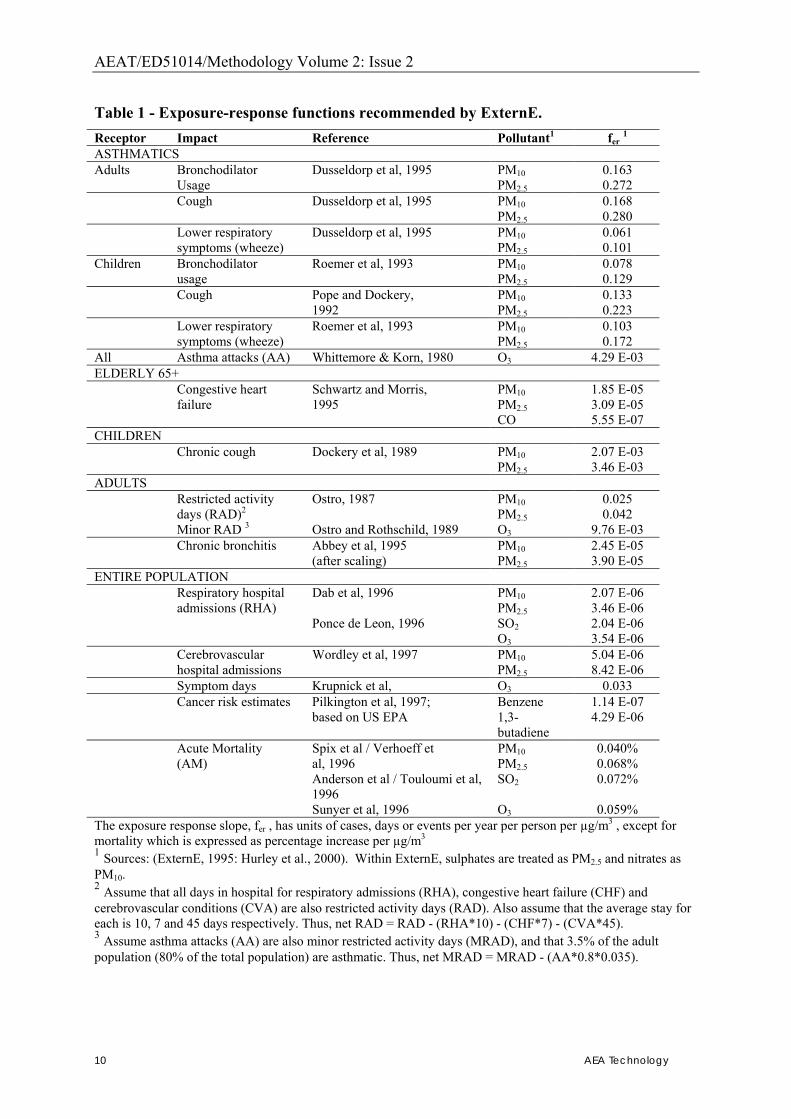
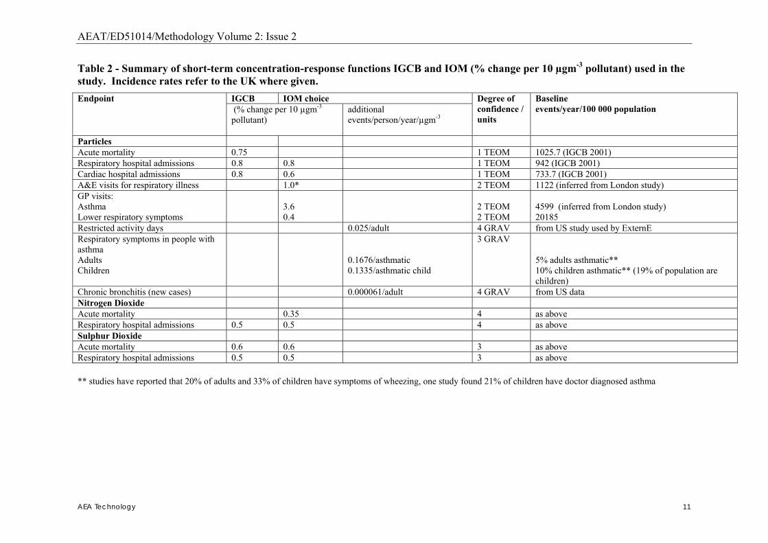
the C-R functions. We were also guided by the principle of coherence; i.e. by considering whether the endpoints being linked with any given pollutant make sense in relation to one another. For example, if pollutants such as PM or ozone are linked with severe health effects (i.e. life-shortening or emergency hospital admissions), and �mild� health effects (such as respiratory symptoms or small reductions in lung function), then is it reasonable to assume that intermediate health effects such as restricted activity days, (RADs) or visits to a family doctor are also affected by these same pollutants. This strengthens the case for attempting to quantify a relationship between air pollutants and RADs, even if the specific epidemiological evidence for that pathway is limited. The dose-response functions recommended by ExternE include mortality due to primary particles (PM2.5 or PM10), nitrates, sulphates, SO2, ozone, benzene and butadiene. Functions for morbidity were recommended for particles, CO, SO2 and ozone. The functions recommended by ExternE, in addition to deaths brought forward and respiratory hospital admissions, are shown in Table 1 below. Table 2 provides the functions used in a slightly later study for the Scottish Executive (IOM and AEA Technology, 2003). These are included here for illustrative purposes only, to show what kinds of impact pathways have been quantified previously. Although used as a starting-point for discussion for the CAFE CBA; they were by no means intended as the last word on the issue.
AEAT/ED51014/Methodology Volume 2: Issue 2
10 AEA Technology
Table 1 - Exposure-response functions recommended by ExternE. Receptor Impact Reference Pollutant1 fer 1 ASTHMATICS Adults Bronchodilator Dusseldorp et al, 1995 PM10 0.163 Usage PM2.5 0.272 Cough Dusseldorp et al, 1995 PM10 0.168 PM2.5 0.280 Lower respiratory Dusseldorp et al, 1995 PM10 0.061 symptoms (wheeze) PM2.5 0.101 Children Bronchodilator Roemer et al, 1993 PM10 0.078 usage PM2.5 0.129 Cough Pope and Dockery, PM10 0.133 1992 PM2.5 0.223 Lower respiratory Roemer et al, 1993 PM10 0.103 symptoms (wheeze) PM2.5 0.172 All Asthma attacks (AA) Whittemore & Korn, 1980 O3 4.29 E-03 ELDERLY 65+ Congestive heart Schwartz and Morris, PM10 1.85 E-05 failure 1995 PM2.5 3.09 E-05 CO 5.55 E-07 CHILDREN Chronic cough Dockery et al, 1989 PM10 2.07 E-03 PM2.5 3.46 E-03 ADULTS Restricted activity Ostro, 1987 PM10 0.025 days (RAD)2 PM2.5 0.042 Minor RAD 3 Ostro and Rothschild, 1989 O3 9.76 E-03 Chronic bronchitis Abbey et al, 1995 PM10 2.45 E-05 (after scaling) PM2.5 3.90 E-05 ENTIRE POPULATION Respiratory hospital Dab et al, 1996 PM10 2.07 E-06 admissions (RHA) PM2.5 3.46 E-06 Ponce de Leon, 1996 SO2 2.04 E-06 O3 3.54 E-06 Cerebrovascular Wordley et al, 1997 PM10 5.04 E-06 hospital admissions PM2.5 8.42 E-06 Symptom days Krupnick et al, O3 0.033 Cancer risk estimates Pilkington et al, 1997; Benzene 1.14 E-07 based on US EPA 1,3-
butadiene 4.29 E-06
Acute Mortality Spix et al / Verhoeff et PM10 0.040% (AM) al, 1996 PM2.5 0.068% Anderson et al / Touloumi et al,
1996 SO2 0.072%
Sunyer et al, 1996 O3 0.059% The exposure response slope, fer , has units of cases, days or events per year per person per µg/m3 , except for mortality which is expressed as percentage increase per µg/m3
1 Sources: (ExternE, 1995: Hurley et al., 2000). Within ExternE, sulphates are treated as PM2.5 and nitrates as PM10. 2 Assume that all days in hospital for respiratory admissions (RHA), congestive heart failure (CHF) and cerebrovascular conditions (CVA) are also restricted activity days (RAD). Also assume that the average stay for each is 10, 7 and 45 days respectively. Thus, net RAD = RAD - (RHA*10) - (CHF*7) - (CVA*45). 3 Assume asthma attacks (AA) are also minor restricted activity days (MRAD), and that 3.5% of the adult population (80% of the total population) are asthmatic. Thus, net MRAD = MRAD - (AA*0.8*0.035).
AEAT/ED51014/Methodology Volume 2: Issue 2
AEA Technology 11
Table 2 - Summary of short-term concentration-response functions IGCB and IOM (% change per 10 µgm-3 pollutant) used in the study. Incidence rates refer to the UK where given.
IGCB IOM choice Endpoint (% change per 10 µgm-3 pollutant)
additional events/person/year/µgm-3
Degree of confidence / units
Baseline events/year/100 000 population
Particles Acute mortality 0.75 1 TEOM 1025.7 (IGCB 2001) Respiratory hospital admissions 0.8 0.8 1 TEOM 942 (IGCB 2001) Cardiac hospital admissions 0.8 0.6 1 TEOM 733.7 (IGCB 2001) A&E visits for respiratory illness 1.0* 2 TEOM 1122 (inferred from London study) GP visits: Asthma Lower respiratory symptoms
3.6 0.4
2 TEOM 2 TEOM
4599 (inferred from London study) 20185
Restricted activity days 0.025/adult 4 GRAV from US study used by ExternE Respiratory symptoms in people with asthma Adults Children
0.1676/asthmatic 0.1335/asthmatic child
3 GRAV 5% adults asthmatic** 10% children asthmatic** (19% of population are children)
Chronic bronchitis (new cases) 0.000061/adult 4 GRAV from US data Nitrogen Dioxide Acute mortality 0.35 4 as above Respiratory hospital admissions 0.5 0.5 4 as above Sulphur Dioxide Acute mortality 0.6 0.6 3 as above Respiratory hospital admissions 0.5 0.5 3 as above ** studies have reported that 20% of adults and 33% of children have symptoms of wheezing, one study found 21% of children have doctor diagnosed asthma
AEAT/ED51014/Methodology Volume 2: Issue 2
12 AEA Technology
1.5.2 Using international or local C-R functions; transferability of C-R functions
Air pollution research has been carried out in many cities in Europe, notably but not only in those cities that have been part of APHEA. The question arises, when quantifying effects in these cities, whether the C-R functions to be used should be based on local studies or on the international literature. Our starting-point is the ExternE position where the approach has been to base the main C-R functions on the international literature as a whole, with preference for studies carried out in Europe, rather than on local studies. However, even for local assessments, we have used the international literature for primary assessments, and have encouraged the use of local functions in supplementary/ sensitivity analyses. The main reasons for this strategy are that:
i. The evidence from studies internationally is, for most impact pathways, far more powerful than from an individual study;
ii. There in a remarkable degree of consistency of findings in epidemiological results internationally, even from studies with important differences in population, climate and pollution mixture;
iii. To a great extent, where differences in C-R functions between locations have been found, the reasons for these differences are not well-understood.
iv. Where the two approaches give different answers, we think it best that the difference be transparent and addressed, even if there is no clear or established explanation.
Number (iii) above is a rather crude generalisation. There are some patterns of difference that have been well-established; for example, in time series studies of daily variations in mortality and hospital admissions, the estimated attributable effect of particles is higher in locations with higher average NO2. We have sought, where possible, to take account of such differences in sensitivity analyses, even if only to see whether they make an important difference to final results. There are some corresponding issues of choice of scale in estimating background rates of morbidity (incidence, prevalence)
1.6. Quantifying the effects of mixtures: the role of specific pollutants
General considerations regarding the effects of mixtures have been considered earlier. In this Section we summarise briefly current thinking on the role of specific components of the general urban air pollution mixture in causing health effects. This includes some discussion of the role of particles of various kinds within the PM10 range. Our emphasis here is not on a general discussion of the role of the various constituents of general urban air pollution � this has been done e.g. by WHO, in its answers to the CAFE questions. Rather, our focus is on how best to incorporate current thinking on toxicity into plans for quantification, which we see as constructing a suitable model for representing approximately the effects of a complex mixture.
AEAT/ED51014/Methodology Volume 2: Issue 2
AEA Technology 13
1.6.1 Attributing effects to particles or to the gases Again, we think that the strategic position adopted by ExternE (1995, 1999) remains a good starting-point and one which is still generally well-supported by evidence. There, when constructing a model of the effects of air pollution, we adopted a staged approach to the inclusion of pollutants.
a. We included first the impact pathways linking ambient PM to a wide variety of cardio-respiratory endpoints, to capture the effects both of daily variations in ambient PM (�acute� effects, or more correctly effects of acute exposure) and of longer-term exposure to PM (�chronic� effects, or more correctly effects of chronic exposure). The reason was that the weight of evidence pointed to some aspect of particles as the primary �driver� of the effects of the pollution mixture as a whole. This was done, of course, only for mixtures where particles were a component of the mixture being evaluated. (Note that an evaluation of changes in NO2 or SO2 requires considering the effects of the derived secondary particles � nitrates and sulphates.)
b. To these we added the effects of ozone, but only for daily variations, not for longer-term exposure; and for respiratory morbidity health endpoints, not cardiovascular ones. The reason was that in many acute studies, there was/is an association between health and ozone which seems to be relatively independent of (and so may be considered as additive to) the effects of PM. There are some studies showing or suggesting that longer-term exposure to ambient ozone may also have adverse effects on health, but we did not attempt to quantify this.
c. Whether or not to further add some impact pathways in SO2 was a difficult choice. We did not do so in primary analyses in 1995. We did in 1999, for a limited number of �acute� respiratory endpoints, though with some doubts about whether the associations implemented are causal in SO2.
d. Similarly for NO2, though both in 1995 and 1999 we did not include pathways in NO2 in our primary analyses. This reflects a view that while there are may be some direct effects of NO2 on health at ambient concentrations, the associations with daily variations in NO2 identified in epidemiology are more likely to reflect the action of more complex mixtures, especially from traffic. Again, there is limited evidence that long-term exposure to NO2 may have some adverse health effects, but we do not think that this justifies quantification.
e. Similarly for CO, where associations may well reflect an effect of �mobile source pollution� generally, rather than of CO in particular.
It is clear from the work both of WHO and of DIEM that there is uncertainty in any attribution of the effects of mixtures to specific pollutants. However, this �hierarchy� of attribution to pollutants is similar to that which is being proposed by the US EPA in quantifying the benefits of the US Clean Air Act; and we think it is still the best way forward for quantification.
1.6.2 Attributing effects of PM to specific types or fractions of particles Ambient PM is something like a mixture, because it varies over time and location in terms of characteristics such as size, composition and surface properties, which are known or believed to influence toxicity. Exactly what characteristics of ambient particles most influence their toxicity continues to be a matter of discussion and of major research interest among air pollution scientists and policy makers.

AEAT/ED51014/Methodology Volume 2: Issue 2
14 AEA Technology
While it might be premature to speak of a consensus on this difficult issue, there is a discernible coalescence of informed opinion around a position somewhat as follows:
a. There is very substantial evidence of adverse health effects of particles measured in mass terms (PM10, PM2.5).
b. There has long been a view that �small particles from combustion sources� may be the main driver, not just of the health effects of these relationships in PM10 and PM2.5, but indeed of ambient air pollution more generally.
c. It is unclear whether, for estimating health effects, such particles are best measured in terms of mass or of number or of surface area. However, for quantification, there are insufficient data (from epidemiological studies; about background and incremental pollution) to permit quantification in metrics other than mass.
d. Evidence is coalescing that, with fine particles from combustion sources, toxicity resides especially in the primary particles, as opposed to the secondary particles (sulphates, nitrates) formed in the atmosphere from emissions of combustion gases.
e. In general, toxicologists are more sceptical than epidemiologists about the adverse effects of secondary particles. This reflects differences in toxicological evidence. • There is substantial epidemiological evidence of associations between health and
sulphates. In these studies sulphates may of course be a marker for other aspects of the mixture, rather than a direct causal agent. They do suggest however that if sulphates are reduced, as part of the reduction of a mixture, then there will be real benefits to health.
• There are many fewer epidemiological studies showing relationships between nitrates and health. This may be due at least in part to difficulties in measuring nitrates.
f. Adverse health effects of coarse particles (represented as PM10-2.5) should not be discounted, because many studies of acute exposure (daily variations) have shown associations. However, effects of long-term exposure of coarse particles on mortality have not been established clearly.
There is however a reluctance to try to translate these insights into quantification rules. We understand this is the position of WHO�s advice to CAFE, and the US EPA is proposing not to try to quantify by source. ExternE has made some 1st beginnings in trying to reflect in its quantification some differences in effects of ambient PM, according to type and nature of the particles. Specifically,
i. effects of sulphates and of primary particles have been estimated as if these particles have, per unit mass (i.e. per µg/m3) the same toxicity as ambient urban PM2.5;
ii. effects of nitrates and of primary particles from power stations and of nitrates have been estimated as if these particles have, per unit mass, the same toxicity as ambient urban PM10.
We think that some differentiation along these lines is useful, although:
• the specifics of the ExternE approach should be reviewed; and • we are mindful of the caveats that should be applied to any such approach.
Though we stress this will only be as part of the sensitivity analysis, and depends on the availability of pollution data that allows source separation.
AEAT/ED51014/Methodology Volume 2: Issue 2
AEA Technology 15
Quantification for the Baseline Report will focus on the effects of a mixture which is not source-specific, and so can avoid reaching a position on differentiation. For the Baseline Report the following position is taken:
a) quantification of PM morbidity effects are investigated both in respect of the metric PM10 and PM2.5, with a final decision on the relevant metric decided upon after the health review process.
b) effects on life expectancy of long-term exposure to particles are quantified in the metric of PM2.5, reflecting the specific evidence of this pathway.
1.7. Particular issues for assessment of mortality
1.7.1 Different kinds of studies identify the mortality effects of acute and chronic exposure
Two types of epidemiological study are relevant to the quantification of mortality impacts from air pollution:
• Time series studies, available for assessment of the short term (acute) mortality impacts through exposure to fine particles, SO2, O3 etc., observe day to day changes in pollution levels with changes in daily death rates. As noted above, the strongest associations are with particles; associations with ozone are being reviewed; and the role of other gaseous pollutants is unclear. Sensitivity analysis around the effect of inclusion or exclusion of these pollutants from the benefits analysis is advisable.
• Cohort studies examine age-specific death rates (technically mortality hazards) in study groups of individuals followed up over prolonged periods. Having adjusted for the influence on mortality of other factors measured for individuals (gender, race, smoking habit, educational status and so on), differences in age-specific death rates between cities are assessed against average pollution concentrations over periods of several years. The key epidemiological studies here are those by Pope et al (1995, 2002), Dockery et al (1993) and Abbey et al (1999). The re-analysis by Krewski et al (2000) of the earlier studies by Dockery and by Pope is also very relevant, because of its comprehensiveness.
In recent years time series studies have been extended to provide information on effects on mortality up to several weeks after air pollution changes, rather than just in the days immediately following.
1.7.2 Cohort and time series studies provide different kind of information about mortality; what metric should be used?
The two types of study provide different types of information a. Time series studies provide results in terms of changes in the number of daily deaths
associated with air pollution. Aggregated over days, these results can be represented as the number of �extra� deaths per annum, attributable to air pollution. These are sometimes described as the number of deaths brought forward, to indicate that in at least some of these cases, the actual loss of life is likely to be small � the death might in any case have occurred within the same year.
b. The most natural implementation of the cohort study results is based on the use of life-tables (see Hurley et al, 2000; WHO, 2000; IIASA, 2002). These use the cohort study estimates together with the demographic characteristics of the �target� population to
AEAT/ED51014/Methodology Volume 2: Issue 2
16 AEA Technology
provide an estimate of the change in life expectancy across the population. Results are expressed in terms of the total number of life years lost for that population, but do not say how many people are affected. This is problematic for valuations based on the value of statistical life (VSL) concept (see below).
Can the approaches be reconciled? There have been a number of attempts at providing information in a common metric.
a. The time series studies do not provide direct information about how many years of life expectancy are lost in these deaths. However, it is widely understood that only those with very vulnerable cardio-respiratory health will have earlier mortality because of higher daily pollution. On that basis, informed estimates on the loss of life expectancy can be and have been made (e.g. ExternE 1999). Strictly, these are speculative, but they allow time series results to be valued in terms of life-years.
b. Early implementation of cohort study results provided information in terms of �extra� deaths per year. This was done by taking the PM-related relative risk from the cohort studies, applying it to the annual death rate in the population and then using the �extra� annual deaths as a measure of the effects of air pollution. This type of analysis is flawed, as it ignores the fact that, if more people die in year 1, there are fewer people at risk in year 2, and so on, with errors accumulating over time.
c. Some experts are currently considering whether the life table methods can be used to derive the number of �extra� deaths associated with chronic exposures. This can be done if a fixed time-frame over which �extra� deaths are to be evaluated is given or can be agreed.
d. Another approach attempts to derive the number of �extra� or attributable deaths based on (i) the total loss of life-years across the population and (ii) the typical loss of life expectancy for those diseases affected by air pollution. Such an approach is described below. Estimates of between 5 and 20 years have been made by various sources. Its status is also speculative.
All of these approaches have been considered in the development of methods described below.
1.7.3 Which type of evidence has priority? Can cohort and time series results be added?
When quantifying impacts caused by particles in a cost-benefit framework it is now standard practice to quantify effects from cohort studies as the principal and most accurate representation of the effects of particles on mortality. This has been the ExternE position for several years (e.g. ExternE, 1999). It is also what the US EPA is proposing to do in its benefits assessment of the Clean Air Act. In principle, cohort studies should capture the full mortality effects of PM. On that basis, it would involve double-counting to add the PM-related mortality effects as estimated from time series studies. In practice, it may be that some aspects of the PM-attributable mortality identified by time series studies are not incorporated into the relative risk estimates of the cohort studies. In particular, this may apply to deaths brought forward by only a few days. Omission of time series estimates will then lead to some under-estimation of the total mortality impact.
• If mortality is expressed and valued in terms of LYL, this gap is of little or no consequence since the �missed� time series deaths are of very low duration of life lost.
AEAT/ED51014/Methodology Volume 2: Issue 2
AEA Technology 17
• On the other hand, if mortality is presented as premature deaths (valued highly irrespective of length of life lost), the impact would be considerable. Nonetheless, it is questionable to attach a high VSL to a life with very short remaining life expectancy.
It is less clear whether or not the time series estimates of mortality in relation to the gases should be assessed and
i. Added to the cohort study estimates of particles, if PM is also part of the mixture being assessed; or
ii. Quantified separately as a mortality impact, if PM is not part of the mixture being assessed.
US EPA proposes not to add time series mortality effects of the gases to the cohort mortality effects of PM. This was the starting position for the CAFE CBA also. For the analysis, where PM is part of the mixture being assessed, cohort study estimates of PM effects will in any case be the dominant ones. Infant mortality A possible problem with the mortality assessment as described here arises because the populations studied by Pope et al (1995, 2002) and by Dockery et al. (1993) are adults, aged more than 25 or 30 years. Other studies show effects on mortality of infants; as noted earlier, we include quantification of this endpoint.

AEAT/ED51014/Methodology Volume 2: Issue 2
18 AEA Technology
2. Specific Decisions on Methodology – General Issues
2.1. Introduction This chapter describes the health impact assessment (HIA) to be undertaken within the Cost Benefit Analysis Contract for CAFE (within CAFE CBA). It also sets out our approach for valuation of the health impacts quantified. It is an edited and enlarged update of the corresponding Section (Appendix 5, Part 2) of the July 2004 Methodology Report (http://europa.eu.int/comm/environment/air/pdf/cba_methodology_issue3.pdf). The present update and revision follows a wide consultation on the July 2004 draft, with comments received from many organisations and individuals; and in particular, a formal peer review where health aspects were reviewed by Dr. Bart Ostro of the California EPA.
2.1.1 Status Note that the present report, though detailed, is not a complete protocol for HIA work to be done within CAFE.
• Some core analyses of the relationship between air pollution and mortality will be carried out within the RAINS model. We do, however, describe the relationship between the HIA work within CAFE CBA and within RAINS, and what extensions of the work within RAINS will be examined here in sensitivity analyses.
• It is possible that elements of the HIA work will be extended further during the implementation phase of CAFE CBA, for example:
o where methodological development is under way currently, either in the scientific community generally, or within the CAFE CBA team, or both; or
o in the choice of C-R function or baseline data for some endpoints, if preliminary analyses suggest that they are especially important, i.e. that they have a substantial impact on final results; or
o if important new information becomes available.
2.1.2 Structure of this health report We begin, as usual, with some framework issues. The following sections then define the approach for:
i. Quantifying mortality, principally in adults; ii. Valuing mortality, principally in adults;
iii. Quantifying mortality in infants and children; iv. Valuing mortality in infants and children; v. Quantifying morbidity, in adults and children;
vi. Valuing morbidity, in adults and children.
AEAT/ED51014/Methodology Volume 2: Issue 2
AEA Technology 19
2.2. Framework Issues
2.2.1 Note on terminology: Acute and chronic exposure and effects As is very well known, epidemiological studies of air pollution and health examine the effects on humans of air pollution experienced over various time periods.
a. Most studies examine the effects of acute exposure; i.e. the ways that air pollution on a given day or adjacent days affects the health of people on the same day or on the days immediately following � typically within one week. (Some analyses of acute exposure now include effects that occur up to 40 days from the relevant pollution days.) The health effects associated with acute exposure to air pollution are often known as acute health effects. This is a well-established abbreviation though possibly a confusing one unless it is made clear that it is the exposure, not the effects, that are acute. (The phrase �acute effects� suggests that the effects are transient. Some may be; some, most notably mortality, are clearly not.)
The US EPA in 1995 summarised the evidence on acute exposures and health as strong evidence for a small increase in risk, a summary description which is still useful. Of course, even small increases in risk, if experienced by many people, can have large public health impacts.
b. A more limited set of studies examines the relationships between health and long-
term (i.e. chronic, possibly lifetime) exposure, and so the associated impacts are often known summarily as �chronic effects�. Although the weight of evidence regarding the effects of chronic exposure is growing, still it is less than that for the effects of acute exposure. However the estimated impacts are greater � both for mortality and morbidity. This is because the effects of long-term exposure encapsulate, at least partially, the effects of daily variations in air pollution that comprise acute exposure, but they also include aspects which are not captured by (i.e. are more than the aggregate of) the effects of daily variations.
With these caveats we will, for brevity, often refer to �acute� and �chronic� effects.
2.2.2 General principles of HIA The general principles underlying HIA work, as it applies to the health impacts of ambient air pollution, have been developed and described in various reports. These include:
• Two reports from the World Health Organisation (WHO); • The Chapters on Public Health in the two Methodology Reports from ExternE (Vols 2
and 7 in the ExternE series) • The Report from the HIA Working Group of AIRNET (in preparation) • The 3-country study on transport by Künzli et al. (2000) • Various Reports from the US EPA, especially those relating to the Second Prospective
Analysis � Benefits and Costs of the Clean Air Act, 1990-2020 • Reports from the APHEIS team • A report by and for the National Science Council in the USA • The report by Hurley et al. (2000) prepared for the Department of Health in London.
AEAT/ED51014/Methodology Volume 2: Issue 2
20 AEA Technology
Our conclusions for HIA within CAFE CBA draw on this accumulated body of experience, to some of which we have contributed over the years. The decisions made are, we think, generally consistent with the guidance from that body of experience. We highlighted and discussed some of the most pertinent of these principles in Issue 2 of the CAFE CBA Methodology Paper (February 2004; op cit), and these are set out above in Chapter 1. We begin with some further discussion of general issues of principle.
2.2.3 Existing reviews Areas of judgement needed in carrying out HIA of the effects of air pollution Any implementation of HIA requires judgements and recommendations about:
a. Hazard identification, and in particular what impact pathways are most relevant. (By impact pathway we mean the linkage between emission of one pollutant and one health endpoint.)
b. Of the pathways identified for for quantification; decisions are needed in the following areas:
i. What concentration-response (C-R) function will be used; ii. What population it applies to (e.g. whether the C-R function applies only to
specific age-groups, or to people with a defined chronic disease such as asthma);
iii. What (estimates of) background rates of mortality or morbidity in the target population will be used;
iv. Any specific issues in implementation � this applies in particular to aspects that are recognised as complex, such as the use of life tables in estimating mortality;
v. How the C-R function links with: • The measures of pollution that are available and being used; • The estimates of background rates; and • The monetary valuations to be applied
c. An assessment of uncertainty in the impacts quantified d. An evaluation of the importance of impacts omitted
Our use of existing reviews As well as drawing on the general body of HIA work on air pollution and health for its general principles, the methods defined here draw heavily on existing reviews of air pollution and health, and on other HIA studies. This is partly because many of these other studies and reviews have already been through detailed processes of peer review and acceptance. However, extensive new review work has been undertaken in the development of this report. Within this framework we highlight some sources in particular. 1. WHO’s “Systematic Review of Health Aspects of Air Quality in Europe”. This consists
of, and is often referred to, as Answers to Questions asked by the CAFE Steering Group. These reviews encompass the health effects associated with or caused by particulate matter (PM), ozone (O3) and nitrogen dioxide (NO2), but not sulphur dioxide (SO2) or carbon monoxide (CO). They consist of a 1st review (http://www.euro.who.int/document/e79097.pdf) and answers to follow-up questions (http://www.euro.who.int/document/e82790.pdf). These reviews are invaluable in
AEAT/ED51014/Methodology Volume 2: Issue 2
AEA Technology 21
providing comprehensive and up-to-date assessments of a whole range of hazard identification framework issues concerning these pollutants and health. The WHO answers to CAFE are not, however, a �tool-kit� for HIA of the effects of air pollution. Rather, the WHO answers to CAFE give a general framework for understanding how PM, O3 and NO2 variously and together impact on human health. There is scope for discretion, and need for judgement, in how these framework understandings translate into the �implementation rules� that are necessary for HIA. We hope and intend that our recommendations are consistent with the WHO answers to the CAFE questions � strongly consistent with them for main implementations and at least weakly consistent with them for sensitivity analyses.
2. Meta-analyses for WHO and CAFE on the effects of acute exposure to PM and to ozone: One aspect of the WHO work for CAFE that was geared especially to quantification is a set of meta-analyses of the acute effects of PM and ozone based on studies in Europe (http://www.euro.who.int/document/e82792.pdf). This work � often referred to in this Report as �the WHO meta-analysis� � was carried out by Ross Anderson and colleagues in London, working as a WHO task group in support of WHO�s Systematic Review. It considers the evidence from studies in Europe of particulate matter expressed variously as PM10, PM2.5, coarse fraction (CF; i.e. PM10 less PM2.5) and black smoke (BS) � all expressed as 24-hr daily average; and of ozone, expressed as 8-hr daily maximum. The meta-analysis reviews studies of acute exposure to these pollutants in relation to a range of �acute� health effects:
• Mortality from all causes, excluding accidents; and cause-specific mortality � respiratory causes, cardiovascular causes;
• Daily numbers of respiratory hospital admissions (including emergency department and emergency room admissions) by broad age-group (0-14 yrs, 15-64, 65+); and daily numbers of hospital admissions for cardiovascular disease (at age 65+);
• Separately for children and adults with underlying respiratory disease: i. Cough
ii. Respiratory medication use
The systematic review found insufficient studies in Europe (i.e. studies of acceptable quality in at least four different European cities) to perform a formal meta-analysis of effects associated with many of its intended impact pathways, including:
• PM2.5, or the coarse dust fraction, for any of the health endpoints studied; • Cough or medication use in symptomatic adults, hospital admissions for
cardiovascular causes at age 65+, and respiratory hospital admissions for children, for any of the pollutant indices studied; and
• Some other pollutant-endpoint combinations.
However, in the text Anderson and colleagues report meta-analysis results based on three studies or fewer, and they suggest that �It may be appropriate to reconsider the guideline on the number of estimates required for a meta-analysis given the small numbers [of studies] available for some combinations of health outcome and pollutant�. We have used results from these �informal� meta-analyses, and occasionally conducted ones of our own, for pathways where there is good evidence of an effect, but limited studies in Europe on which to base quantification.
AEAT/ED51014/Methodology Volume 2: Issue 2
22 AEA Technology
3. We pay particular attention to recommendations regarding quantification from the WHO Task Force on Health (TFH) providing support to the UNECE Convention on Long-Range Trans-Boundary Air Pollution (LRTAP). This is important for CAFE because the recommendations of WHO-TFH were designed for implementation within the RAINS model of IIASA; and RAINS includes HIA estimates of the effects of PM and ozone respectively on mortality. The relationship between the intentionally limited HIA work within RAINS and the intentionally more extensive HIA work within CAFE CBA is discussed further below.
4. The work of ExternE and of Hurley et al. (2000) because most of the CAFE CBA team
was formed within ExternE and became consolidated with work also for the UK Department of Health; and so, from that experience, bring a �tradition� of quantification to the present project.
5. The work of Künzli and colleagues (2000), this being another major European
‘tradition’ of health impact assessment for air pollution 6. Current or recent work on major projects such as:
• APHEIS: http://www.apheis.net/ • the WHO Global Burden of Disease project:
http://www3.who.int/whosis/menu.cfm?path=evidence,burden • The Second Prospective Analysis by the US EPA of the Benefits and Costs of the
Clean Air Act, 1990-2020: See: • http://www.epa.gov/air/sect812/blueprint.html for extensive documentation of the
EPA�s Draft Analytical Plan; and • http://www.epa.gov/sab/pdf/council_adv_04002.pdf for a response from the
Health Effects Sub-Committee of the Special Panel, set up to advise on the analysis.
In all of this we acknowledge an influence of Bart Ostro of the California EPA who pioneered the use of many of the methods of quantitative HIA for ambient air pollution and who acted as formal designated reviewer of the HIA within CAFE CBA.
2.2.4 HIA work within RAINS and for the benefits analysis of CAFE CBA Although what we conclude here for CAFE CBA is consistent with the HIA work within RAINS, there are many differences also. In particular CAFE CBA includes
(i) estimates of morbidity impacts, and so looks at a much wider range of health endpoints than RAINS;
(ii) additional analyses of mortality; (iii) monetary valuation; and (iv) assessment of uncertainties, including of impact pathways that we have not been
able to quantify. These differences, which arise because the HIA work has a different purpose within RAINS and within the CBA Benefits analysis, were recognised and discussed at the May 2004 meeting of the TFH of WHO-LRTAP in Bonn � see especially paragraphs 25, 28, 29 of the relevant minutes at http://www.unece.org/env/documents/2004/eb/wg1/eb.air.wg1.2004.11.e.pdf. The
AEAT/ED51014/Methodology Volume 2: Issue 2
AEA Technology 23
differences and the complementary nature of the two HIAs are described in more detail below.
Purpose of HIA in RAINS � studying cost-effectiveness across different policies to reduce pollution RAINS was developed initially and is still used primarily as an integrated assessment methodology and tool for analysis of cost-effectiveness. That means its primary purpose is to:
• Consider specific air quality objectives or environmental or health targets; and then • Identify what policy or policies can meet these targets in the most cost-effective way
according to the set of measures contained within the RAINS database. In that context, HIA within RAINS enables an analysis of cost-effectiveness when air quality objectives or targets are set in terms of reductions in mortality, for example, reductions in attributable deaths or in average life expectancy. From the viewpoint of HIA within RAINS, the key point is that quantification of health effects is part of a process designed to compare and evaluate the costs of different strategies to reduce pollution to achieve specified targets Whilst cost-effectiveness analysis identifies efficient ways of meeting targets it does not answer the question of whether it is worthwhile meeting those targets. Purpose of HIA in Benefits Analysis for CAFE CBA � comparing costs and benefits of specific policies to reduce pollution The CBA work within CAFE, and so HIA within that CBA work, has a different purpose. Here, the quantification of health effects is part of a process designed to compare and evaluate the costs and benefits of specific strategies. In other words, the results of a CBA will show whether or not a given policy will generate net benefits and as such be justifiable. CBA, however, does not on its own provide information on whether the policies considered are an efficient way of improving environmental quality. Implications of the differences in purpose These differences in purpose have implications for the kind of HIA strategy that is needed in the two contexts. Given that both involve HIA work within the CAFE programme, we think it is important to spell out these differences in strategy, so that differences in detail between the approaches can be understood. a. How comprehensive the HIA needs to be and how strongly based in evidence Within HIA work, there is always a trade-off between how comprehensive the quantification is (i.e. how wide a range of pollutants is considered, and how wide a set of endpoints is included for each pollutant) and how strongly the quantification is based in evidence. Briefly, there are two main traditions in HIA. Both are legitimate; but they are appropriate for different purposes.
i. One tradition puts priority on ensuring that every impact pathway that is included has been quantified reliably, with estimates based strongly in the available evidence. This tradition aims to include only those impact pathways where quantification can be based on strong and direct evidence, where there is a broad consensus that the evidence is reliable, and so where reliable concentration-response (C-R) functions are available. It is reluctant to extrapolate beyond the available data. It makes no claim to capture the full effects of air pollution, but it can be strong in its confidence about the effects that are quantified.
AEAT/ED51014/Methodology Volume 2: Issue 2
24 AEA Technology
The work of COMEAP (1998) in the UK is in that tradition, as is the work of APHEIS and the Global Burden of Disease. It is an important tradition for asserting with confidence that air pollution causes damage at least as great as that which is quantified, and that reductions in pollution lead to widely accepted quantifiable benefits. HIA within RAINS is also within that tradition � this was recognised explicitly at the May 2004 meeting of WHO-TFH. This is the correct basis for comparing different air pollution policies from the viewpoint of cost-effectiveness.
ii. Another tradition puts priority, not so much on the reliability of each individual
pathway that is included, but on the reliability of the quantification as a whole as an estimate of the overall benefits of reducing air pollution. Thus, while it is important that individual pathways are quantified as reliably as practicable � especially those that have a major impact on the �bottom line� of the benefits analysis as a whole � this needs to be balanced against how comprehensive (complete) the HIA is, in total; i.e. to what extent it captures all of the effects on health of the air pollution mixture of interest, or at least the large majority of the health impacts that have any substantial impact on the �bottom line� of benefits assessments. A basis in evidence remains essential, but there is a greater willingness for that evidence to come from fewer studies, or to be indirect (e.g. via arguments of mechanisms), or to involve extrapolations, conversion factors and other assumptions that are strictly uncheckable. This is because it is difficult to take unquantified benefits into account; and so it may better to include an inexact quantification than to not quantify at all.
The work of ExternE, of Künzli et al., of the US EPA is largely in this tradition. It is an important tradition, and the relevant one for establishing the benefits of air pollution reductions when these are to be compared with costs. We proposed in the earlier draft paper (February 2004) that this is the more appropriate tradition for HIA within CAFE CBA. This is because, in comparing benefits of reducing pollution with costs, a HIA which confines itself only to those impact pathways and strategic judgements which can be supported with strong confidence will lead to exclusion of many impact pathways where air pollution does have an effect, but its size is known less reliably. This in turn leads to under-estimation of the effects as a while, and to a strategy which is in practice anti-precautionary.
iii. These traditions can be seen as complementary, not in conflict; and that is the viewpoint taken by the various participants in CAFE. Specifically:
• The pathways that underlie the �conservative� HIA, and the associated judgements regarding their implementation, can form a solid core for the main analyses of the more expansive CBA work.
• This core can and should be augmented in two ways: o By including additional pathways where the evidence is less strongly
based than in the �conservative� HIA model; o By examining, at least in sensitivity analyses, the practical
importance of varying some assumptions which for the core model might be seen as insufficiently based in evidence.
AEAT/ED51014/Methodology Volume 2: Issue 2
AEA Technology 25
iv. The approach we are taking in CAFE CBA leans towards the �expansive� tradition,
though possibly not as fully as we have done elsewhere (e.g. ExternE, 1999). We augment the �core� RAINS model HIA with an extensive range of other health endpoints; we do more sensitivity analyses; but do not try � at least at this stage � to include all possible pathways. Rather, we focus on those pathways which results from other studies have identified as most important in contributing to monetised benefits. Some pathways, which may be relevant but where the evidence is weak, are included in sensitivity analyses only. One use of this limited sensitivity analysis is to see whether or not these pathways are potentially important.
b. Annualisation and monetary valuation in the CAFE CBA work Because RAINS is about comparing the health effects of different pollution reduction policies, the key requirement is that the comparisons between pollution reduction strategies be carried out on a common basis. Exactly what that basis is, is less important than its reliability. For example, a comparison can be valid irrespective of whether the effect being quantified is a sustained change in air pollution or a short-term �pulse� change. And there is no need to move to monetisation The situation in CAFE CBA is different. Here, the focus is on comparing costs and benefits of specific policies to reduce air pollution. It is essential that costs and benefits be compared on some common basis. That common basis includes:
• Monetary valuation of the benefits to health and • Common accounting time-frame for the evaluation of costs and benefits. This can be
in terms of annualisation; i.e. ensuring that one year�s costs in pollution reduction are compared with the benefits of one year�s reduction in pollution. It can also be in examining the present value of costs or benefits of a policy.
Both of these are issues that are addressed in the present protocol.
2.2.5 Mixtures, attributing effects to specific pollutants, including which particles
In the February 2004 draft of the Methodology Report we discussed the issues of air pollution mixtures and some associated questions relevant to HIA. We re-visit these here, to describe what we will do in CAFE CBA.
i. To what extent can the associations between air pollution and health, which are widely accepted as causal in respect of the air pollution mixture as a whole, realistically be considered as causal also with regard to specific air pollutants?
This question is important when developing a suitable set of C-R functions for use in HIA. In CAFE CBA we are concerned in particular with health effects associated with ambient particulate matter (PM), represented as PM2.5 or PM10, and with health effects associated with ambient ozone. Consistent with the evaluations of WHO, and in particular with the recommendations of WHO-TFH regarding thresholds, the working position of the present report is that: • there are causal relationships between ambient PM and a wide range of cardio-respiratory
health effects; • those causal relationships are captured imperfectly, but sufficiently for quantification, by
concentration-response (C-R) functions in the metrics of PM2.5 and/or PM10;
AEAT/ED51014/Methodology Volume 2: Issue 2
26 AEA Technology
• at the population level there is no �safe� threshold level of anthropogenic PM; • ambient ozone is causally related to cardio-respiratory mortality and a wide range of
respiratory (though not cardiovascular) morbidity endpoints; • daily 8-hr max O3 is a suitable metric for quantifying ozone effects; and that • while there is no known threshold for the adverse effects of ambient ozone, there is only
weak information about effects at low concentrations, and so it is prudent to quantify health effects only for periods when ambient O3 exceeds a cut-off point of 35 ppb (8-hr daily max), with effects without a cut-off point being estimated in sensitivity analyses only.
ii. To what extent is it reasonable to aggregate estimated impacts across pollutants? The working viewpoint taken in the present report is that: • it is reasonable to add together the estimated health impacts of PM and of ozone; • while there may be advantages in using C-R functions where the estimated effects of PM
and of ozone are adjusted each for one another (for those endpoints where effects of both pollutants are estimated), it is not essential to do so, because estimated effects from two-pollutant models are often similar to estimated effects from single-pollutant models.
• with further addition of impacts associated with other pollutants � SO2, NO2, CO � there is a danger of double-counting, especially with the estimated effects of PM.
These viewpoints partly reflect the thinking on causality, earlier. In part they also reflect that SO2 and NO2 tend to be more highly correlated with PM and with one another than with ozone. The formal review advised care if effects in NO2 and/or SO2 and/or CO were to be estimated and added to the effects of PM and O3. Recent evidence from the US NMMAPS study supports the view that adjustment for PM makes little change to all-year estimates of the effects of O3 on mortality. Results from APHEA2 in Europe suggest that this overall favourable effect may arise because of different patterns in summer and winter: the PM-adjusted coefficient for O3 is lower in summer, higher in winter, than the corresponding unadjusted coefficient, leading to a similar all-year estimated effect.
iii. Other than by distinguishing particles in terms of size – PM10, PM2.5 (fine particles), PM10–PM2.5 (coarse particles, sometimes written PM10-2.5) – to what extent is it useful and possible to apply different risk estimates to particles differentiated by composition, surface properties and source? Alternatively, to what extent should risk estimates for the general urban particulate mixture in a given size range (PM10, PM2.5, PM10-2.5) be applied to all particles in that size range, regardless of other characteristics of those particles?
The issue arises because there is some evidence that, per µg/m3 pollutant, primary particles from combustion sources have greater toxicity than secondary particles (sulphates, nitrates) of similar size range. Within ExternE we have, for many years, attempted some differentiation (see e.g. ExternE, 1999, Methodology Report 7); in particular, we applied a factor to nitrates that scaled down their estimated health effects relative to those of PM2.5 generally. Applying such a factor is speculative, though indeed not applying a factor is speculative also � there is inadequate epidemiology on which to base directly an estimate of the health effects of nitrate PM specifically. WHO-TFH considered this difficult issue in 2003, as part of its recommendations to RAINS � see http://www.unece.org/env/documents/2003/eb/wg1/eb.air.wg1.2003.11.pdf - and the same question was again more recently considered in detail as part of WHO�s answers to CAFE
AEAT/ED51014/Methodology Volume 2: Issue 2
AEA Technology 27
follow-up questions (http://www.euro.who.int/document/e82790.pdf). The most recent WHO review noted that:
• toxicological studies have highlighted the primary, combustion-derived particles having a high toxic potency;
• several other components of the PM mix � including sulphates and nitrates � are lower in toxic potency; but that
• it is currently not possible to precisely quantify the contributions from different sources and different PM components to health effects from exposure to ambient PM.
Bart Ostro, in his formal review, agreed. In wider consultations (linked to the EU DIEM project, to meetings of AIRNET, and at a workshop as part of the 2004 ISEE Conference in New York) we have found support for the aim of differential quantification, but at present a reluctance, sometimes marked, to attempt to quantify differential effects of similarly-sized particles of different composition. Consequently, it is not practicable at this time for the HIA work of CAFE CBA to differentiate risks of ambient PM by composition, surface properties or source, because: • On the basis of the WHO-TFH recommendation, the modelling within RAINS of changes
in ambient PM arising from various policies has not put priority differentiating PM by characteristics such as source and composition, and so the particulate pollution data are not readily available in a suitably disaggregated form; and
• There is at present no way of quantitatively applying different risk estimates to particles from different sources in the same size range (PM2.5 or PM10) in a way that can be expected to achieve any widespread consensus within the research community on air pollution and health.
However, we believe that this issue is an extremely important one in policy analysis. Recent work at a national level (Watkiss et al, 2005) has used different risk factors for individual components of the PM2.5 fraction, attributing higher risk factors to primary PM and lower risk factors to nitrates (whilst keeping the same overall baseline impacts the same). The analysis then assessed the impact of different policies on top of this baseline scenario using the adjusted risk factors, and compared it to an analysis where equivalent risk factors where the same for all components of the PM mixture. The different approaches produced very different policy benefits between sectors, for example the benefits of transport policies increased by more than a factor of two when adjusted risk factors where used1. For CAFE, at the very least we need estimate to what extent the benefits assessments of various policies are robust or sensitive to different plausible assumptions about the relative toxicity of different parts of the PM mixture. (The main relevant contrast is that of primary particles versus secondary particulate species such as nitrates and sulphates). Quantitative differentiation, if and when it is considered feasible, could have a major impact on estimates of those policies where the composition and source of the reduced PM is markedly different than the composition of urban ambient PM generally � for example, where the reductions target nitrate PM specifically. As well as commenting qualitatively on results, we intend to undertake some sensitivity analyses that specifically explore whether quantifying the different parts of 1 The work, undertaken as part of an �Air Quality Evaluation� showed that the use of different risk factors for particulate matter (assigning lower values to secondary particulates) altered the relative benefits of policies in different sectors, e.g. between the transport sector and electricity generation sector, because of the different proportions of primary PM, and secondary PM precursors by sector. This affected both the benefit to cost ratio of policies, and their cost-effectiveness in delivering health benefits.
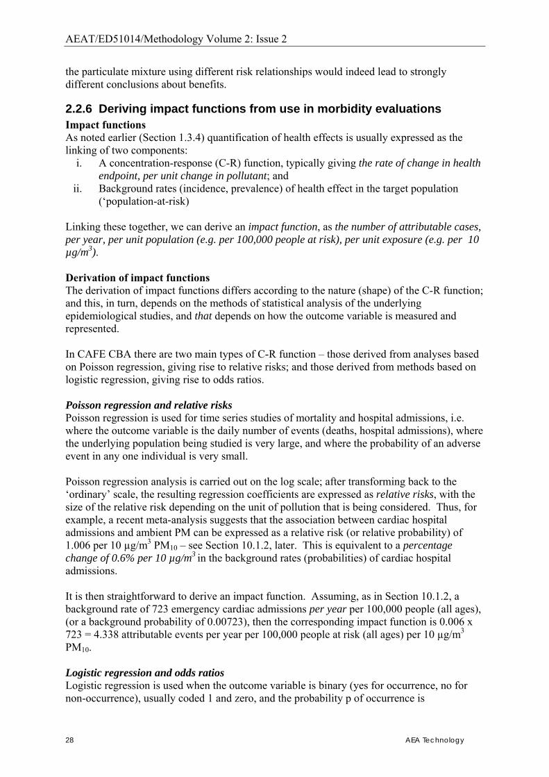
AEAT/ED51014/Methodology Volume 2: Issue 2
28 AEA Technology
the particulate mixture using different risk relationships would indeed lead to strongly different conclusions about benefits.
2.2.6 Deriving impact functions from use in morbidity evaluations Impact functions As noted earlier (Section 1.3.4) quantification of health effects is usually expressed as the linking of two components:
i. A concentration-response (C-R) function, typically giving the rate of change in health endpoint, per unit change in pollutant; and
ii. Background rates (incidence, prevalence) of health effect in the target population (�population-at-risk)
Linking these together, we can derive an impact function, as the number of attributable cases, per year, per unit population (e.g. per 100,000 people at risk), per unit exposure (e.g. per 10 µg/m3). Derivation of impact functions The derivation of impact functions differs according to the nature (shape) of the C-R function; and this, in turn, depends on the methods of statistical analysis of the underlying epidemiological studies, and that depends on how the outcome variable is measured and represented. In CAFE CBA there are two main types of C-R function � those derived from analyses based on Poisson regression, giving rise to relative risks; and those derived from methods based on logistic regression, giving rise to odds ratios. Poisson regression and relative risks Poisson regression is used for time series studies of mortality and hospital admissions, i.e. where the outcome variable is the daily number of events (deaths, hospital admissions), where the underlying population being studied is very large, and where the probability of an adverse event in any one individual is very small. Poisson regression analysis is carried out on the log scale; after transforming back to the �ordinary� scale, the resulting regression coefficients are expressed as relative risks, with the size of the relative risk depending on the unit of pollution that is being considered. Thus, for example, a recent meta-analysis suggests that the association between cardiac hospital admissions and ambient PM can be expressed as a relative risk (or relative probability) of 1.006 per 10 µg/m3 PM10 � see Section 10.1.2, later. This is equivalent to a percentage change of 0.6% per 10 µg/m3 in the background rates (probabilities) of cardiac hospital admissions. It is then straightforward to derive an impact function. Assuming, as in Section 10.1.2, a background rate of 723 emergency cardiac admissions per year per 100,000 people (all ages), (or a background probability of 0.00723), then the corresponding impact function is 0.006 x 723 = 4.338 attributable events per year per 100,000 people at risk (all ages) per 10 µg/m3 PM10. Logistic regression and odds ratios Logistic regression is used when the outcome variable is binary (yes for occurrence, no for non-occurrence), usually coded 1 and zero, and the probability p of occurrence is

AEAT/ED51014/Methodology Volume 2: Issue 2
AEA Technology 29
approximated by the long run relative frequency of occurrences in the long run. In our applications, this can arise in studying chronic disease (e.g. subject did or did not develop symptoms of chronic bronchitis during the study period) or in panel studies of respiratory symptoms or medication usage (e.g. subject did or did not report a particular symptom, or use a bronchodilator, on a given day). Logistic regression also works on the log scale, but rather than working with the log of the probability p, it builds models to represent and explain the log of the odds o, where o = p/(1-p). Note that this implies the corresponding equation p = o/(1+o), where as before p represents probability and o represents corresponding odds. Analysis in terms of (log) odds rather than probabilities has several advantages, especially when the probability can be large. These include that:
• Whereas the probability p is constrained to be no larger than 1, the odds o ranges from 0 to infinity; and so a 10% increase in odds can be applied no matter how large the background odds are; and
• Analyses of (log) odds give similar results, whether attention is focused on an event (reported a symptom) or its converse (did not report a symptom); whereas this is not true when analyses are made of probabilities. For example, if the background rate (daily prevalence) of reporting symptoms is 0.2, then a 10% increase in the probability of reporting symptoms is 0.02. It would be elegant and useful if this corresponded to a 10% decrease in the probability of not reporting a symptom, but it doesn�t, the latter being 0.08, i.e. 10% of 0.8. This characteristic of symmetry does however apply to percentage changes in odds.
Logistic regression coefficients, after transformation back from the log scale, are measures of relative odds (i.e. more commonly called odds ratios, and leading to percentage changes in odds) rather than relative risks (leading, as above, to percentage changes in probabilities). Derivation of an impact function is then somewhat more complicated than for relative risks. We illustrate this by an example � medication use by children with asthma (see Section 10.3.2, following), where logistic regression analyses of one study suggested an odds ratio of 1.41 per 10 µg/m3 O3. The relevant background rate (mean daily prevalence) of bronchodilator usage was 40% i.e. p=0.4.
• The background rate of 0.4 implies an odds of 0.4/(1-0.4), i.e. 0.4/0.6, or 0.666. • With an odds ratio of 1.41 per 10 µg/m3 O3, this gives a new odds of 0.94 • This new odds is equivalent to a new probability of 0.94/1.94, or 0.485, following an
increase of 10 µg/m3 O3. • Thus, and an increase of 10 µg/m3 O3, and an initial background rate of 40%, imply a
new background rate of 48.5% (95% CI 41.2%, 55.8%). • Subtracting the original background incidence rate of 40% from these new figures
gives an increase of 0.085 in the daily probability of usage, or 0.085 x 365 = 31 extra usage days per annum, assuming that a person was at risk throughout the whole year.
Note that:
• For a given odds ratio, the percentage change in probability depends on the background probability � this has implications for transferability of impact functions between locations with different background rates of occurrence; and
• When the background rates are low (say, 10% or less), then there is little difference in absolute terms between a probability (e.g. 0.1) and an odds (e.g. 0.11), and so it is not misleading to apply odds ratios as if they were relative risks.

AEAT/ED51014/Methodology Volume 2: Issue 2
30 AEA Technology
3. Quantification of Mortality
3.1. Introduction As set out in earlier drafts of the CBA Methodology, over time an understanding has emerged of how epidemiological studies of different design can be used to quantify mortality. a. Time series studies of acute exposure lead most naturally to impact estimates in terms of
attributable cases, i.e. the number of extra �deaths brought forward� (or lives shortened) attributable to (changes in) air pollution in the immediately preceding days, aggregated over the entire year.
b. Cohort studies of chronic exposure give results in terms of changes to mortality hazards
(age-specific death rates) per unit change in pollution. For impact estimation, this change in mortality hazards can be most reliably represented by using life table methods to express mortality impacts in the target population in terms of changes in life expectancy and/or in total life-years (LY) gained for given reductions in air pollution.
Chapter 1 also identified a wide range of issues to be addressed and resolved in relation to as part of the HIA for CAFE CBA. Below we set-out the way forward for CAFE CBA, drawing heavily on the advice to RAINS given by WHO-TFH at its meetings of both 2003 (see http://www.unece.org/env/documents/2003/eb/wg1/eb.air.wg1.2003.11.pdf) and May 2004: (http://www.unece.org/env/documents/2004/eb/wg1/eb.air.wg1.2004.11.e.pdf). We consider first the effects of mortality from long-term exposure to pollution. It is well-known that these are the dominant effects in HIA and CBA (e.g. Hurley et al., 2000; Künzli et al., 2000; AEA Technology, 1998; Holland et al, 1999; Rabl, 2003).
3.2. Mortality effects of long-term (chronic) exposure to ambient particles
3.2.1 Choice of effect estimate in terms of % change per unit pollutant Choice of cohort study on which to base effect estimates As noted in the draft from February 2004, we will base estimates on the extended follow-up by Pope et al. (2002) of the American Cancer Society (ACS) cohort. This is consistent with current practice, including, for example, WHO-TFH advice to RAINS; GBD; the Advisory to the US EPA; and Rabl (2003). In other words, the use of Pope et al. (2002) is already becoming standard in air pollution health impact assessments (HIAs), because • The ACS study is the most extensive of the various available cohorts; • The original study findings and methods (Pope et al.,1995) were supported by HEI-
sponsored re-analyses, which examined methodological issues in great detail (Krewski et al., 2000);
• Pope et al. (2002) is based on about 3 times as many deaths as Pope et al. (1995); • Its authors included some of the main statistical analysts of the cohort study re-analysis; • Smaller cohort studies give more extreme estimates � some higher than the most recent
ACS (Pope et al., 2002) estimates, some lower.
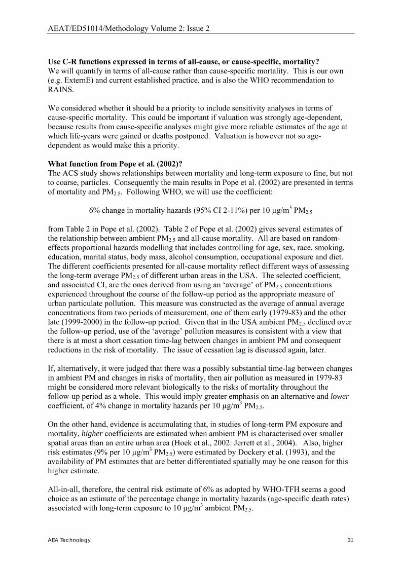
AEAT/ED51014/Methodology Volume 2: Issue 2
AEA Technology 31
Use C-R functions expressed in terms of all-cause, or cause-specific, mortality? We will quantify in terms of all-cause rather than cause-specific mortality. This is our own (e.g. ExternE) and current established practice, and is also the WHO recommendation to RAINS. We considered whether it should be a priority to include sensitivity analyses in terms of cause-specific mortality. This could be important if valuation was strongly age-dependent, because results from cause-specific analyses might give more reliable estimates of the age at which life-years were gained or deaths postponed. Valuation is however not so age-dependent as would make this a priority. What function from Pope et al. (2002)? The ACS study shows relationships between mortality and long-term exposure to fine, but not to coarse, particles. Consequently the main results in Pope et al. (2002) are presented in terms of mortality and PM2.5. Following WHO, we will use the coefficient:
6% change in mortality hazards (95% CI 2-11%) per 10 µg/m3 PM2.5 from Table 2 in Pope et al. (2002). Table 2 of Pope et al. (2002) gives several estimates of the relationship between ambient PM2.5 and all-cause mortality. All are based on random-effects proportional hazards modelling that includes controlling for age, sex, race, smoking, education, marital status, body mass, alcohol consumption, occupational exposure and diet. The different coefficients presented for all-cause mortality reflect different ways of assessing the long-term average PM2.5 of different urban areas in the USA. The selected coefficient, and associated CI, are the ones derived from using an �average� of PM2.5 concentrations experienced throughout the course of the follow-up period as the appropriate measure of urban particulate pollution. This measure was constructed as the average of annual average concentrations from two periods of measurement, one of them early (1979-83) and the other late (1999-2000) in the follow-up period. Given that in the USA ambient PM2.5 declined over the follow-up period, use of the �average� pollution measures is consistent with a view that there is at most a short cessation time-lag between changes in ambient PM and consequent reductions in the risk of mortality. The issue of cessation lag is discussed again, later. If, alternatively, it were judged that there was a possibly substantial time-lag between changes in ambient PM and changes in risks of mortality, then air pollution as measured in 1979-83 might be considered more relevant biologically to the risks of mortality throughout the follow-up period as a whole. This would imply greater emphasis on an alternative and lower coefficient, of 4% change in mortality hazards per 10 µg/m3 PM2.5. On the other hand, evidence is accumulating that, in studies of long-term PM exposure and mortality, higher coefficients are estimated when ambient PM is characterised over smaller spatial areas than an entire urban area (Hoek et al., 2002: Jerrett et al., 2004). Also, higher risk estimates (9% per 10 µg/m3 PM2.5) were estimated by Dockery et al. (1993), and the availability of PM estimates that are better differentiated spatially may be one reason for this higher estimate. All-in-all, therefore, the central risk estimate of 6% as adopted by WHO-TFH seems a good choice as an estimate of the percentage change in mortality hazards (age-specific death rates) associated with long-term exposure to 10 µg/m3 ambient PM2.5.
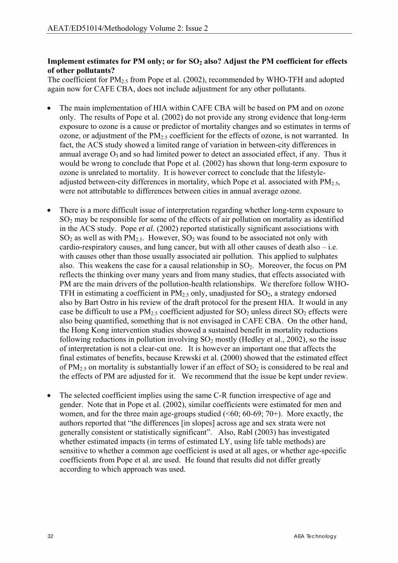
AEAT/ED51014/Methodology Volume 2: Issue 2
32 AEA Technology
Implement estimates for PM only; or for SO2 also? Adjust the PM coefficient for effects of other pollutants? The coefficient for PM2.5 from Pope et al. (2002), recommended by WHO-TFH and adopted again now for CAFE CBA, does not include adjustment for any other pollutants. • The main implementation of HIA within CAFE CBA will be based on PM and on ozone
only. The results of Pope et al. (2002) do not provide any strong evidence that long-term exposure to ozone is a cause or predictor of mortality changes and so estimates in terms of ozone, or adjustment of the PM2.5 coefficient for the effects of ozone, is not warranted. In fact, the ACS study showed a limited range of variation in between-city differences in annual average O3 and so had limited power to detect an associated effect, if any. Thus it would be wrong to conclude that Pope et al. (2002) has shown that long-term exposure to ozone is unrelated to mortality. It is however correct to conclude that the lifestyle-adjusted between-city differences in mortality, which Pope et al. associated with PM2.5, were not attributable to differences between cities in annual average ozone.
• There is a more difficult issue of interpretation regarding whether long-term exposure to
SO2 may be responsible for some of the effects of air pollution on mortality as identified in the ACS study. Pope et al. (2002) reported statistically significant associations with SO2 as well as with PM2.5. However, SO2 was found to be associated not only with cardio-respiratory causes, and lung cancer, but with all other causes of death also � i.e. with causes other than those usually associated air pollution. This applied to sulphates also. This weakens the case for a causal relationship in SO2. Moreover, the focus on PM reflects the thinking over many years and from many studies, that effects associated with PM are the main drivers of the pollution-health relationships. We therefore follow WHO-TFH in estimating a coefficient in PM2.5 only, unadjusted for SO2, a strategy endorsed also by Bart Ostro in his review of the draft protocol for the present HIA. It would in any case be difficult to use a PM2.5 coefficient adjusted for SO2 unless direct SO2 effects were also being quantified, something that is not envisaged in CAFE CBA. On the other hand, the Hong Kong intervention studies showed a sustained benefit in mortality reductions following reductions in pollution involving SO2 mostly (Hedley et al., 2002), so the issue of interpretation is not a clear-cut one. It is however an important one that affects the final estimates of benefits, because Krewski et al. (2000) showed that the estimated effect of PM2.5 on mortality is substantially lower if an effect of SO2 is considered to be real and the effects of PM are adjusted for it. We recommend that the issue be kept under review.
• The selected coefficient implies using the same C-R function irrespective of age and
gender. Note that in Pope et al. (2002), similar coefficients were estimated for men and women, and for the three main age-groups studied (<60; 60-69; 70+). More exactly, the authors reported that �the differences [in slopes] across age and sex strata were not generally consistent or statistically significant�. Also, Rabl (2003) has investigated whether estimated impacts (in terms of estimated LY, using life table methods) are sensitive to whether a common age coefficient is used at all ages, or whether age-specific coefficients from Pope et al. are used. He found that results did not differ greatly according to which approach was used.
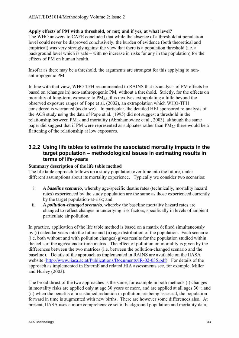
AEAT/ED51014/Methodology Volume 2: Issue 2
AEA Technology 33
Apply effects of PM with a threshold, or not; and if yes, at what level? The WHO answers to CAFE concluded that while the absence of a threshold at population level could never be disproved conclusively, the burden of evidence (both theoretical and empirical) was very strongly against the view that there is a population threshold (i.e. a background level which is safe � with no increase in risks for any in the population) for the effects of PM on human health. Insofar as there may be a threshold, the arguments are strongest for this applying to non-anthropogenic PM. In line with that view, WHO-TFH recommended to RAINS that its analysis of PM effects be based on (changes in) non-anthropogenic PM, without a threshold. Strictly, for the effects on mortality of long-term exposure to PM2.5, this involves extrapolating a little beyond the observed exposure ranges of Pope et al. (2002), an extrapolation which WHO-TFH considered is warranted (as do we). In particular, the detailed HEI-sponsored re-analysis of the ACS study using the data of Pope et al. (1995) did not suggest a threshold in the relationship between PM2.5 and mortality (Abrahamowicz et al., 2003), although the same paper did suggest that if PM were represented as sulphates rather than PM2.5 there would be a flattening of the relationship at low exposures.
3.2.2 Using life tables to estimate the associated mortality impacts in the target population – methodological issues in estimating results in terms of life-years
Summary description of the life table method The life table approach follows up a study population over time into the future, under different assumptions about its mortality experience. Typically we consider two scenarios:
i. A baseline scenario, whereby age-specific deaths rates (technically, mortality hazard rates) experienced by the study population are the same as those experienced currently by the target population-at-risk; and
ii. A pollution-changed scenario, whereby the baseline mortality hazard rates are changed to reflect changes in underlying risk factors, specifically in levels of ambient particulate air pollution.
In practice, application of the life table method is based on a matrix defined simultaneously by (i) calendar years into the future and (ii) age-distribution of the population. Each scenario (i.e. both without and with pollution changes) gives results for the population studied within the cells of the age/calendar-time matrix. The effect of pollution on mortality is given by the differences between the two matrices (i.e. between the pollution-changed scenario and the baseline). Details of the approach as implemented in RAINS are available on the IIASA website (http://www.iiasa.ac.at/Publications/Documents/IR-02-035.pdf). For details of the approach as implemented in ExternE and related HIA assessments see, for example, Miller and Hurley (2003). The broad thrust of the two approaches is the same, for example in both methods (i) changes in mortality risks are applied only at age 30 years or more, and are applied at all ages 30+; and (ii) when the benefits of a sustained reduction in pollution are being assessed, the population forward in time is augmented with new births. There are however some differences also. At present, IIASA uses a more comprehensive set of background population and mortality data,
AEAT/ED51014/Methodology Volume 2: Issue 2
34 AEA Technology
for implementation across Europe; whereas our implementation gives much greater flexibility in choice of output. Also, we use 1-yr groupings both for age and for calendar time, IIASA uses 5-yr age groups; we follow up for more than 100 years, IIASA until 2075; IIASA uses real population projections for new births, we assume that future years will be the same as the starting year. These relatively minor differences in methodology lead to minor differences in results also. We discuss below what characteristics of the results might usefully be summarised. Methodology for expressing the impact of pollution on mortality hazard rates The change in mortality hazard rates attributable to pollution is expressed by increasing (or decreasing) the age/calendar-year mortality hazard by a defined percentage. This is the natural way to reflect pollution-related changes, because the C-R functions from the air pollution cohort studies such as Pope et al. (2002) were obtained using proportional hazards statistical modelling. The percentage change applied to the mortality hazard rates can vary from one cell to another; i.e. it can vary by age of population, or by calendar year in the future, or both. This gives great flexibility in modelling two different kinds of assumption. • It allows flexible modelling of different kinds of pollution change � for example, a
pollution change that is sustained long-term, or pollution that is changed for a fixed period only (pulse change).
• It also allows flexible modelling of different assumptions or results concerning how a given change in pollution may affect age-specific death rates in the population. This includes (i) modelling the time-lag between a change in pollution and a change in population hazard rates and (ii) allowing the change in hazard rates to vary with age. (Note that in our application, the % change in mortality hazard rates is the same at all ages.)
Results are linear in the extent (percentages) by which mortality hazard rates are changed. For example, if the percentage change applied to each cell was doubled, then all results would change by a factor of two also. In practice, this means that results are linear in µg/m3 changes in PM2.5. Different kinds of populations which may be studied using life table methods In applying life table methods to a target population, the population studied (i.e. the population to which the life table methods are applied) can be defined in a number of different ways. The three most common kinds of study population are:
a. It can be a birth cohort that experiences the same hazard rates as the population of interest. The birth cohort is followed up until everybody in it has died.
b. It can be the currently-alive population of interest. Again, follow-up is until everybody in the currently alive population has died.
c. It can be the currently-alive population augmented by new births each year. This is a mixture of �a� and �b�, above. With new births each year, there is no obvious cut-off point in the future for the end of mortality follow-up.
Choice of what is the most appropriate kind of population depends on the nature of the policy question being considered. We give some examples, below. Other considerations may, however, apply also, in particular the need to compare across costs and benefits of one or more policies.
AEAT/ED51014/Methodology Volume 2: Issue 2
AEA Technology 35
Studying the effects of a sustained change in pollution When policies are introduced to reduce pollution, there is usually an intention of maintaining that reduction long-term. Those who will experience reduced pollution are, therefore, the entire currently exposed population and all those newly born in that location in future years; i.e. a �mixture� population as in option �c�, above. (We assume zero net migration.) Typically, we have followed up mixture populations for about 120 years; i.e. beyond the lifetime of the longest living of the current population. By doing so, results for a birth cohort (�a� above) and for the currently-alive population (�b� above) can be derived from the results of the mixture population. This can be done by summarising over the appropriate subset of cells of the matrix age/calendar-year matrix (see e.g. Miller and Hurley, 2003; Hurley et al., 2000). Studying the effects of a 1-yr �pulse� change in pollution It is usual, however, when studying the costs and benefits of a change in pollution, to standardise the comparisons so that what is compared are annualised costs and benefits; i.e. the costs and benefits of a 1-yr change in pollution. There are three approaches to doing this.
i. Study the effects of a 1-yr �pulse� change in pollution. Here the appropriate study population is the cuurently-alive population (�b�, above), because it is only those currently alive who expereince a 1-yr pulse change in pollution.
ii. Study the effects of a sustained change, and divide by the number of years over which the change has been assessed, to derive estimates of annual benefits.
iii. Change the comparison of costs and benefits so that they are compared on a long-term, not an annual, basis.
Option (iii) has a lot to recommend it. It is, however, not the approach that is usually adopted currently. • Methodological work suggests that Options (i) and (ii) give similar results in terms of
estimated impacts expressed as life-years lost or gained. From the viewpoint purely of impacts, choice between the two approaches may be a matter of convenience.
• Option (i) is simpler in that only the currently exposed population experiences a change in pollution. Thus, as noted above, the relevant kind of population to study is population Type �b�, above. This implies that estimates of future new births are not needed.
• The pleasing similarity between the two approaches in terms of estimated life-years no longer applies if and when the impacts are linked with monetary valuation (except in the special case of zero discount rate). This is because there is a very different distribution over time of the life-years associated with a 1-yr pulse (applied to the current population) compared with the life-years from a sustained pollution reduction (applied to a population including new births). The former occur substantially earlier, on average, and so on average they are affected less by discounting of monetary values.
For CAFE CBA we will use results from sustained pollution changes, supplemented by analyses of �pulse� changes in pollution: the advantages of the latter for cost-benefit comparisons outweigh the fact that a 1-yr �pulse� change is a somewhat artificial option in practice. For further discussion of the concepts of �pulse� and �sustained� changes in air pollution, see also by Rabl (2003).
AEAT/ED51014/Methodology Volume 2: Issue 2
36 AEA Technology
Latency, or time-lag to effect While there are some more-or-less immediate effects of air pollution on mortality, other effects are probably delayed.
• That some effects are immediate follows from the fact that associations between air pollution and daily deaths are detected by time series studies. By design, these studies detect only those effects that occur in the immediately preceding days, typically no more than one week.
• More recent developments, known as distributed lag models, allow exploration of relationships with a time-lag of several weeks. These models provide higher estimates of relative risks per µg/m3 pollutant than time series studies using shorter lags.
• It is expected that a longer time-lag applies to the relationship between long-term exposure to air pollution and the development of chronic cardio-respiratory disease; and, probably, a still longer time-lag between exposure and any lung cancer that may be attributable.
• The extent of such time-lag or latency is unknown � in particular, the cohort epidemiological studies which provide estimates of relative risk (RR) are uninformative about time-lag � but plausible distributions of latency can be constructed.
Many HIAs that use cohort studies assume no time-lag between changes in pollution and consequent changes in death rates. This is the approach taken by RAINS and, for consistency, we will adopt this also for the core analyses for CAFE CBA. We will also carry out sensitivity analyses based on various assumed time-lags between changes in pollution and changes in death rates. For example Hurley et al. (2000) explored a wide range of possible cessation lags. Our work will draw on recent discussions informing the US EPA�s analysis of the costs and benefits of the US Clean Air Act (see e.g. http://www.epa.gov/sab/pdf/council_hes_background_info_092104.pdf) where, for examole, one option being discussed is that (say) 30% of the effect of reduced pollution on deaths rates occurs immediately (year1); 50% of the effect is distributed over years 2-5; and the remaining 20% is distributed over years 6-20. Results, in terms of life-years, are relatively independent of age-distribution and mortality hazard rates of the target population We know both from empirical and from theoretical work that, when standardised for population size (e.g. LY per 100,000 of the current population-at-risk), results are largely independent of:
• The age-structure of the population studied; • The age-specific death rates experienced by the population studied.
Certainly this applies within the ranges of variation in age-distribution and in mortality rates experienced in Europe. This allows two simplifications.
• First, it is not necessary to model carefully any changes in age-specific mortality rates in the future.
• Secondly, results per unit population (e.g. per 100,000 people at risk) can be transferred from one population to another � it is not necessary to re-do the life-table calculations for each target population of interest.
AEAT/ED51014/Methodology Volume 2: Issue 2
AEA Technology 37
On that basis, we have carried out preliminary results based on the population of England and Wales (about 55 million people). We consider that these results are more generally applicable to the European population. We will, however, seek to verify this directly, in the course of CAFE CBA.
3.2.3 Using life tables to estimate the associated mortality impacts in the target population – illustrative example: context, methods and results for a 1-yr pulse change
Population: We studied the population of England and Wales in 1999. The total population studied was 52.516 million people. All results were divided by 525.16 to give values per 100,000 population-at-risk Mortality follow-up: Mortality follow-up was from 1999 to 2120 � i.e. until beyond the time when all those alive in 1999 had died. Pulse change (1-yr) or sustained change in pollution? Include new births or not? The results presented here refer to a pulse change. For this, we assume a 1-yr reduction in pollution. The pollution change applies only to people currently alive. The population studied is therefore the currently alive population only. Background death rates (i.e. without pollution-related changes) in future years: We have assumed that current death rates will continue to apply in future years. This is unrealistic. However, we have shown that the estimated effects of pollution changes on life-years are insensitive to different assumptions about future death rates (e.g. Hurley et al., 2000). This reflects a more general phenomenon, noted above, that results (e.g. per 1% change in death rates) vary only a little by age-distribution and death rates of the population studied. Migration: We assume zero migration. Gender: Age-specific death rates, and the age-distribution of the population in any given calendar year, are different for women and for men. Consequently, the life tables were applied separately for men and women. Results are given for the two genders combined. This is because, despite the differences in death rates, results (for the same % change in death rates, say 1% change) are very similar for both women and for men � see also above. Disaggregation by age and calendar time: Calculations are based on a matrix of age-group and calendar time, using 1-yr cell grids in both dimensions. Changes in death rates: Results were calculated and are presented for a 1% change in death rates. This is the effect on mortality of 1.67 µg/m3 PM2.5, if we use a coefficient from the ACS study of 6% per 10 µg/m3 PM2.5. More intuitively perhaps, results 6 times those given refer to a change of 10µg/m3 PM2.5. The same % changes were applied to age-specific death rates for women and for men. Changes were applied at age 30 upwards, only. At ages 30 or more, the same % change was applied at each age group Time-lag to effects: In the present example, we assumed that the mortality risks (totalling a 1% change in death rates) were �phased in� over a period of 11 years, with some immediate
AEAT/ED51014/Methodology Volume 2: Issue 2
38 AEA Technology
effects and some spread over the following 10 years. This is not proposed as the most realistic phasing in � we will examine other options � but it does illustrate the possibilities. Specifically, for a 1-yr pulse change in pollution, we assumed corresponding changes in mortality hazards (at ages 30 years or more) of:
• 0.4% in Year 1; • 0.06% in each year from Year 2 to Year 11, inclusive. (Note � this is not
cumulative. The actual value for each of those years is 0.06% difference from baseline).
• Reverting to baseline after Year 11 and staying at baseline thereafter. Scaling for other values of percentage change: The results scale linearly in percentage change, if other things are kept equal. Thus, results from a sensitivity analysis using a coefficient of 4% change in death rates per 10 µg/m3 PM2.5 can be obtained by simple scaling. Results, in terms of life-years: Results showed a total of 57, 028 life years gained for a 1% reduction in death rates, phased-in as described. The life-years are gained only by people aged 30 years or more, but we present the results per all-ages population of 52.5 million people. Taking the WHO-recommended coefficient of 6% reduction in age-specific death rates (hazard rates) per 10µg/m3 PM2.5, this is equivalent to:
• 108.6 years per 100,000 people (all ages) per 1.67 µg/m3 PM2.5 reduction in pollution for 1 year;
• 65.1 years per 100,000 people per µg/m3 PM2.5 reduction in pollution for 1 year • 0.2376 days per person per µg/m3 PM2.5 reduction in pollution for 1 year
Comparison with other estimates: These results are broadly similar to those obtained and reported by Rabl (2003). Are the life-years gained (saved) experienced in good health, or not? If we look on air pollution as causing �accelerated aging�, including earlier disease, these are healthy LY. If we think it �simply� hastens death in people with existing disease, then these are less healthy years, but not necessarily disabled ones. Probably there is a mixture. The issue needs discussion. Our presumption is towards healthy life-years.
3.2.4 A comparison of the CAFE approach with that used by the WHO Global Burden of Disease Project
In the last two years, estimates of the mortality effects of chronic exposure to fine particles by the WHO Global Burden of Disease (GBD) Project (see Ezzati et al, 2002) have become a focus for European decision makers. Ezzati et al report European impacts to be equal to 107,000 deaths and 725,000 years of life lost2. Analysis covered 51 countries. Other quantifications in Europe have generated larger estimates. The CBAs of the NEC and Ozone Directives and the Gothenburg Protocol estimated as many as 3 million years of life lost (AEA Technology, 1998; Holland et al., 1999) to fine particle exposure across Europe, though they did not include all sources of particle. Kunzli et al (2000) estimated 40,000
2 Ezzati et al (2002) describe the 725,000 figure in units of DALYs (Disability Adjusted Life Years), but is understood that the units for this number should be years of life lost. The corresponding DALY estimate is 849,000.
AEAT/ED51014/Methodology Volume 2: Issue 2
AEA Technology 39
deaths in only 3 countries � a rate double that of the GBD results when expressed per head of population considered in the two studies. It is similarly anticipated that the estimate of chronic effects on mortality to be made in the CAFE programme will be substantially higher than the GBD estimate for several reasons, including:
• The total population addressed by CAFE is much higher than that considered by GBD. This is because GBD focussed o urban air pollution, and so estimated impacts in populations of cities of >100,000 people. Thus, for example, for the Region EUR-A (comprising much of the EU25) GBD considered impacts in 80 million people. In CAFE CBA, for the EU25, exposure of around 450 million people will be considered. Going further, the UNECE domain of the RAINS model contains a population of nearly 800 million.
• Both studies use coefficients from Pope et al. (2002). However, whereas CAFE CBA uses an estimates of 6% change in all-cause mortality hazards per 10µg.m-3
PM2.5, GBD uses cause-specific results equivalent to a 4% change in all-cause mortality.
• The conversion factor of 0.5 used to convert PM10 to PM2.5 also appears conservative from a European perspective. CAFE (and GBD sensitivity analysis for Europe) uses a factor of 0.65 where necessary, based on observations from various sources in Europe and North America.
There are also differences in the range over which the two studies quantify effects of particles:
• The GBD analysis only quantifies beyond 15µg.m-3 PM10, taken as equivalent to 7.5µg.m-3
PM2.5. CAFE does not quantify with a cut-off point as such, but includes only anthropogenic contributions to PM2.5 concentrations, excluding secondary organic aerosols. The overall effect of this difference is not clear.
• The use of an upper bound concentration of 50µg.m-3 PM2.5 would seem to make no
difference to the CAFE results, as initial concentration data received by the CBA team indicate that this level is not reached in the modelled domain, with highest concentrations reaching only 36µg.m-3
PM2.5 (anthropogenic, excluding secondary organics).
From discussion with the authors of the GBD report we are confident that these differences reflect the separate objectives of the GBD Project and CAFE, rather than fundamentally different views about health impact assessment methodology between the authors of the two studies.
3.2.5 Moving towards valuation In terms of the physical impacts quantified, CAFE CBA will be consistent with the guidance from WHO, and the output from the RAINS model, and express chronic mortality effects in life years in the first instance. For many years it has been the study team practice (see e.g. ExternE 1999) to work principally in terms of life years for valuation as well as physical impacts. For CAFE CBA we have however been asked to express mortality benefits, from cohort studies, in terms of �attributable deaths� also (or, for pollution reductions, attributable deaths delayed). The reason for this request is because the Valuation of a Statistical Life (VSL) was considered to be more reliable than the Value of a Life Year (VOLY), as the latter has historically been derived computationally from the former. As will be detailed in the next section, there is now better empirical information concerning the VOLY, from two new monetary valuation studies. We have attempted to express results in terms also of attributable cases (avoided),
AEAT/ED51014/Methodology Volume 2: Issue 2
40 AEA Technology
despite Rabl (2003) arguements that it is not possible to estimate attributable cases in a meaningful way. Expressing results in terms of deaths rather than life years We describe two possible approaches to estimating numbers of deaths (attributable cases) associated with long-term exposure to PM.
• The first approach attempts to use life tables, because this is the methodology used to give results in terms of life expectancy. As far as we know, life tables are not used currently to estimate �attributable deaths�. Indeed, there are some important methodological problems in attempting to do so. Our description indicates the problems and the possibilities of overcoming them.
• The second approach does not use life tables. It is simple to implement and is widely used. It is however an over-simplification and, as such, over-estimates effects to some extent � see below.
1) Estimating deaths using a life-table approach What metrics to use in expressing mortality impacts: life-years or deaths? Each cell of the life table age/calendar-year matrix gives results in terms of:
i. Life-years lived ii. Deaths
In principle therefore, we can summarise results in either metric. Differences between the changed and baseline scenarios can be expressed in terms of life-years gained (or lost), as we have done above; or in terms of �extra� (or fewer) deaths, at different ages or time-periods in the future. If it does not matter at what age, or at what time in the future, that deaths occur, or life-years are gained or lost, then it is possible to aggregate results over age-groups, or calendar time, or both, and so provide summary results. Trivial but important result in terms of numbers of deaths There is however a danger of trivialisation in considering and aggregating results in terms of numbers of deaths. Because in the long run everybody dies, and dies once only, the aggregate number of deaths in a birth cohort (�a� above) or in the currently-alive population (�b� above) will be exactly everybody in that birth cohort or population, irrespective of the effects of pollution on mortality. This highlights the possibly obvious fact that information about pollution and mortality does not reside not in the fact of death � this is taken as being certain � but rather in its timing: how soon will death occur? Timing of death simultaneously affects both age at death and calendar year, and so affects also person-years of life lived. Aggregate person-years of life will therefore differ between baseline and pollution-changed scenarios, even if a population is followed to extinction, and so aggregate deaths are the same under both scenarios. This is why we have preferred to express results in terms of life-years lost (or gained) rather than �extra� (or �fewer�) deaths. Expressing results (from analyses of a birth cohort or of the currently alive population) in terms of numbers deaths is meaningful if: • Deaths at younger ages are seen as more, or less � usually more � important (valuable)
than deaths at older ages. Note this issue is also relevant for the valuation of a year of life lost. If the value of life year changes according to age � and there is some evidence to suggest that the value might increase with age � then it has important implications for the

AEAT/ED51014/Methodology Volume 2: Issue 2
AEA Technology 41
alternative methodological approach using VOLYs.Then, deaths can be expressed by age-group rather than overall, and the baseline and pollution-changed scenarios will differ because under higher pollution, age at death will on average be somewhat lower; or
• Deaths many years ahead are seen as more, or less important than deaths in immediately upcoming years. It is usual to consider future deaths as being less important, an effect implemented via a non-zero rate of time preference. Then, deaths can be expressed by calendar-time in the future rather than overall, and the baseline and pollution-changed scenarios will differ because under higher pollution, deaths will on average occur sooner than under lower pollution.
Of course, both aspects may simultaneously be considered to be important. Thus, while there are no extra deaths overall, there can be and are extra (or fewer) deaths in various age-groups and time periods; and this can have a non-zero value overall. For a sustained pollution reduction, then the aggregated number of deaths will be higher under higher pollution than under reduced pollution. This appears to overcome the problem of zero differences in deaths, discussed above. However Rabl (2003) argues persuasively that the number of deaths obtained by such calculations has no easy interpretation in terms of attributable cases. 2) Estimating deaths using a �static� approach There is a simpler approach to estimating attributable cases, without using life tables. This approach was used by ExternE in 1995; its use is still widespread (e.g. Künzli et al., 2000; US EPA � various). It is based on a simple calculation: Take
annual death rate x population size x %increase per µg/m3 PM2.5 x change in PM2.5 and call these the attributable deaths, applying a VSL to each. It is usual to implement this approach without a time-lag, though a time-lag could be introduced. The strengths of this approach are that (i) it is easy to do and (ii) it is easy to understand and to communicate, if it is accepted that these are �attributable cases�. The main weakness is that strictly speaking it is wrong (i.e. at best, an approximation). � Under higher air pollution, higher deaths in one year lead to a different population-at-risk
in the next year, and so on. This accumulation of impacts on population structure can appear small in any one year, but can accumulate over time.
� This approach is equivalent to that derived from life tables, if we estimate only the deaths under a higher pollution scenario and do not compensate by subtracting the value of those same deaths when they would have occurred, later, under reduced pollution.
� It will therefore be seen that this approach over-estimates the mortality impacts to some extent.
This second approach has been used in the CAFE quantifications.
AEAT/ED51014/Methodology Volume 2: Issue 2
42 AEA Technology
Conclusions and recommendation Results expressed as life-years The cohort studies lead �naturally� to results expressed in terms of life years gained in total or on average, across the population at risk. The distribution of life years across individuals in the population is unknown and possibly unknowable. It is consistent with the guidance given by WHO, and the metrics used from RAINS in the cost-effectiveness analysis. Results expressed as attributable cases • Calculations from life tables can give results in terms of numbers of deaths. For a pulse
change in the current population, there is no change in the overall number of deaths � everybody dies, once. The difference is that under lower pollution, people on average die somewhat older and somewhat later, so if VSL is age-related, and/or a non-zero rate of time preference is used, there is a difference in monetary valuation between the higher-pollution and lower-pollution scenarios.
• Also, estimates in terms of numbers of deaths can be obtained in a simple way that avoids the use of life tables. This approach over-estimates effects, since it fails to take into account that �extra� deaths under higher air pollution are in fact deaths postponed, not avoided; and so the VSL at point of death under higher pollution should be offset by the VSL later, when the death would have occurred under lower pollution.
• In CAFE CBA we will use this simpler method because (i) it is both simple to do and, despite its limitations, is widely-used; and (ii) the methodological problems associated with using deaths from life tables have not been tackled and resolved sufficiently for us to use the methods at this point.
• These methodological differences imply that there is no easy equivalence or �conversion� between the estimates of life years and attributable deaths in CAFE CBA, even though both are derived using the same coefficient from the US cohort studies, and using the same pollution data. In particular, it is not valid to �convert� between life years and deaths, from the results of CAFE CBA.
Concluding remarks The estimation of attributable cases from cohort studies remains difficult and controversial, despite approaches that appear to provide easy ways of making the estimates. The health impact community strongly favours using life-years rather than attributable cases. However, as the peer review of the CBA methodology pointed out, the methodology of valuing the life years is problematic. This value of life year (VOLY) is computed in an ad hoc manner from the value of statistical life (VSL). As the estimate of value of statistical life is more easily defended from a theoretical perspective, the peer review recommended that we make our best effort to calculate the attributable cases so that the VSL can be applied to this. Thus, we have done this, too, using a widely used, simple but approximate approach.
3.2.6 Should (some of) the effects of PM as estimated from time series studies be added to the PM effects as estimated from cohort studies?
This issue is one where there is currently no clear-cut answer. See also, for example, the Advisory to the US EPA Benefits Analysis for a fuller discussion. Briefly, it appears that while in principle the cohort studies should indeed capture the mortality effects that time series studies capture, in practice it is likely that they do not do so fully. This view, which has been argued on general grounds, is supported by the fact that
AEAT/ED51014/Methodology Volume 2: Issue 2
AEA Technology 43
whereas time series studies clearly show a relationship between ambient PM and mortality from respiratory causes, the cohort studies do not � see, e.g., the detailed report of the HEI-sponsored re-analysis (Krewski et al., 2000). Nevertheless, adding time series effects for PM to cohort study effects risks double-counting. We will follow ExternE, and WHO advice to RAINS, and not do this. This advice is consistent with current practice in impact estimation. On the other hand, we have decided to make some estimates of the �acute� effects of PM on mortality, i.e. the effects on mortality as estimated from time series studies. The purpose of this quantification is purely to obtain a view of their magnitude, for comparisons with (i) estimates of the effects of PM, from cohort studies and (ii) estimates of the effects of ozone, from time series studies. For analyses of the �acute� effects of PM on mortality we use the C-R function from the WHO meta-analysis of studies in Europe, giving an estimated change of
0.6% (95% CI 0.4%, 0.8%) per 10 µg/m3 PM10
NB: It is not intended that these time series estimates of mortality associated with PM should be:
• Added to the PM effects of cohort studies � this would lead to probable double-counting; or
• Be used as an alternative to the cohort study estimates � we regard the cohort study estimates as the fundamental ones, a point emphasised also by Bart Ostro in his review.
3.3. Effects on mortality of short-term exposure (acute exposure, daily variations) to ozone
3.3.1 Which pollutants? With respect to short term exposures, we will quantify effects on mortality associated with ozone only. As noted above,
• HIA for CAFE CBA will be based on the effects of PM and ozone; • The mortality effects of PM are captured most comprehensively in the cohort studies; • While there may be some additional effects captured by time series studies, these are
likely to be relatively small; • On that basis, and to avoid double-counting, the PM effects from time series studies
will not be added to the cohort study effects; • This implies that the mortality effects to be included in CAFE CBA from short-term
exposure to air pollution are those related to ozone.
3.3.2 Estimating impacts of ozone reduction in terms of ‘deaths postponed’ (attributable cases avoided)
Again, we will follow the guidance from WHO to RAINS � see previous references to minutes of the relevant Task Force on Health (TFH) meetings in 2003 and 2004. The main points are as follows.
AEAT/ED51014/Methodology Volume 2: Issue 2
44 AEA Technology
• We will estimate effects in relation to daily ozone, characterised as a daily maximum 8-hr mean, in relation to daily all-cause mortality.
• The WHO answers to CAFE follow-up questions found no evidence of a threshold for the effects of ozone on human health. The review acknowledged however that the reliability of assuming effects decreased as the exposures being considered became lower � because the extent of extrapolation beyond the base of evidence became greater at lower ozone concentrations.
• Against that background, WHO-CLRTAP advised RAINS that the main quantification of the relationship of daily ozone with daily mortality should be restricted to quantifying the effects at concentrations greater than 35ppb daily maximum 8-hr mean, on days when the daily maximum 8-hr mean exceeded that level. The acronym SOMO35 (sum of means over 35) was used as shorthand for this measure of daily ozone concentrations.
• Following WHO-CLRTAP, we will use a risk estimate of 0.3% increase in daily mortality (95% CI 0.1-0.4%) per 10 µg/m3 O3 � this is the estimate, unadjusted for publication bias, from the WHO-sponsored meta-analysis of time series studies in Europe. It is based on studies in 15 cities in France, Italy, the Netherlands, Spain and the United Kingdom, estimated without a threshold. Results from APHEA 2 are not included, since they were not published by the time the meta-analysis was conducted. (There is some evidence that with-threshold estimates of the relationship between ozone and acute mortality lead to higher estimated coefficients.) Note that the US EPA is carrying out a meta-analysis of time series studies on mortality and ozone before deciding whether and how to quantify this endpoint in their Benefits Analysis of the US Clean Air Act.
• Note that there have been two very recent publications of the effects of ozone on mortality, one from NMMAPS in the USA (Bell et al., 2004), one from APHEA2 in Europe (Gryparis et al., 2004). We will in the coming period examine the WHO meta-analyses estimates in the light of these new emerging results.
• Ozone effects will be estimated over a full year. • WHO recognised that estimating effects only above a cut-off point is a very
conservative approach to the estimation of the mortality effects of ozone. Consequently, it recommended a sensitivity analysis giving estimates with no cut-off point (or equivalently, with the cut-off point at zero) as an upper bound on the true impacts.
As noted earlier, results are additive to the estimated effects of PM on mortality, as estimated from cohort studies.
3.3.3 Linkage with monetary valuation Previous work by the study team (ExternE 1999, Hurley et al. 2000) has involved �conversion� of attributable deaths from time series studies to equivalent changes in life years. The reason for this choice, as noted earlier, is that for these deaths brought forward (with higher air pollution) or postponed (with lower air pollution) it is misleading to use the full Value of a Statistical Life for monetary valuation, because it attributes the full VSL to what is understood to be only a small portion of a full life expectancy. Put differently, there are many reasons why life is shortened. Air pollution in the days immediately preceding death is but one of them. It is widely understood though not fully established that higher air pollution in the days before death is a contributory factor to earlier death only in people who already have

AEAT/ED51014/Methodology Volume 2: Issue 2
AEA Technology 45
serious cardio-respiratory disease; and it seems reasonable and even necessary to attribute the deaths in greater part to that underlying disease and, perhaps, to the risk factors (smoking, occupation, diet, poverty�) that caused it. This argument is developed concisely by Rabl (2003). Alternatively, application of a full VSL might be appropriate if:
i. It were possible to estimate when the relevant death would have occurred in the absence of air pollution;
ii. The VSL at that future point was calculated at today�s prices, taking account of any age-related differences in VSL and applying discounting;
iii. The pollution-attributable value is taken as the difference between the VSL now and the VSL (at today�s prices) of the life when death would have occurred, in the absence of air pollution;
iv. The age specific change of VSL is known (there is evidence that the value of statistical life does not change until old age implying that the value of life year is increasing correspondingly).
This approach, which avoids the attribution to air pollution of life-shortening from other causes, reflects the fact that there is really no such thing as �lives saved� by lower air pollution. It suggests, yet again, that the �natural� metric is life years rather than deaths. The main complication is lack of direct evidence on (ii) above, about when the death would have occurred in the absence of air pollution. This is the same complication that arises when attempts are made to estimate life years saved when daily pollution levels are lower.
3.3.4 Inferring life years saved Inferring life years saved takes us beyond the direct base of evidence; that is, inferring life years saved involves making assumptions that are speculative, and based on indirect evidence; they cannot be taken directly from studies. (In this, they are similar to assumptions about the time-lag between changes in pollution and changes in death rates, in estimating impacts using results from cohort studies.) There are several relevant facts that are well-established:
• Most deaths are from cardiovascular-related causes; some are from respiratory causes (as primary cause of death);
� Most deaths occur in older people � There is limited evidence, and strong informed speculation, that the pollution-
attributable �extra� daily deaths, in the days following days of higher air pollution, occur only in those with pre-existing severe cardio-respiratory disease.
Severe pre-existing cardio-respiratory disease doesn�t necessarily mean that those at risk are already in hospital. Serious cardiovascular disease can remain undetected, especially in younger people; and so �sudden death� from cardiovascular causes can occur among people living apparently �normal� lives. However, together, these characteristics imply on average a �short� life expectancy among those whose death is triggered by higher air pollution (e.g. ozone) in the immediately preceding days. Can we estimate how short? We can make some inferences.
AEAT/ED51014/Methodology Volume 2: Issue 2
46 AEA Technology
Studies of the time-related patterns of daily deaths in relation to air pollution, to help understand the extent of mortality displacement, show that a proportion would have died very soon anyway. One way of looking at this is to consider that they would have died from the same episode of illness, but in the absence of higher days of air pollution would have survived a little longer. This phenomenon, known somewhat crudely as �harvesting�, applies, however, to only a proportion of the earlier deaths. It is reasonable to consider that, in the absence of higher air pollution days, others would have survived that episode � e.g. recovered from a heart attack � and lived for perhaps months or years longer, before the underlying disease was brought to a point of crisis. Such individuals will have a major effect on the average loss of life expectancy per case, especially where (as here) average is interpreted as arithmetic mean. We have previously speculated (e.g. ExternE 1999, Hurley et al., 2000) that the associated distribution of LY likely to be heavily skewed to the right, i.e. with arithmetic mean substantially higher than median. (It is the mean which is most relevant to impact estimation.) To allow a LY quantification to proceed, we have previously assumed an arithmetic mean of about 6 months (limits 3 months to 1 year), a value also adopted by Rabl (2003), for illustrative purposes. This was considered a high estimate at the time it was made (1998, 2000) but understanding has changed over time. Indeed, Ostro (see peer review comments) thought that 6 months loss of life years, on average, was a low estimate. Levy et al. (2001), speculating similarly to what we have done above and for ExternE, estimated 1 year of life lost per premature death attributable to ozone. In the light of these opinions we consider that a better estimate of the average loss of life expectancy amongst those affected by acute effects of air pollution is around 1 year, and so we take this as our core estimate. The effects of uncertainty in this parameter will be investigated in more depth during the analysis.
AEAT/ED51014/Methodology Volume 2: Issue 2
AEA Technology 47
4. Valuation of Mortality
4.1. Introduction The valuation of air pollution related mortality has been the subject of much debate in recent years. One topic of debate relates to the preference for using the Value of a Statistical Life (VSL) or the Value of a Life-Year (VOLY) and reflects the discussion above on the interpretation of the epidemiological evidence. To date, the empirical basis for monetary valuation of the Value of a Statistical Life (VSL) has been much stronger than that of the valuation of a life-year-lost (VOLY). In the absence of empirical studies, the VOLY is derived from the VSL, using methods that require assumptions about discounting the value of future life-years. However, the derivation of numbers of deaths (especially for chronic mortality analysis) was considered highly uncertain from the perspective of health impact assessment (see previous sections). A need to conduct specific valuation of mortality in an air pollution context was identified in the original ExternE report series, though progress in this area has been relatively slow. This section reviews progress to date, reporting the current position of EC DG ENV on the appropriate metric and unit values. Importantly, it also provides the findings of two new empirical studies undertaken by the EC NewExt project and by UK�s Department for Environment, Food and Rural Affairs (DEFRA). These primary air pollution valuation studies provide a significant advance in this area, and have been used to inform the proposals for the CAFE analysis.
4.2. Metrics for mortality valuation
4.2.1 Value of statistical life Reports from a working group set up by EC DG ENV (2000) to debate valuation of mortality are available on the web. The Working Group�s firm preference was for estimates based on the value of statistical life (VSL). The working group considered evidence on the VSL from wage-risk studies and contingent valuation studies, and considered the latter to be the more robust for defining society�s willingness to pay to reduce risk. The group identified a VSL from research in the UK in 1998, as a baseline figure. This provided a best estimate of �1.0 million for the VSL after converting to � for the year 2000, and adjusting down to account for the age of those likely to be affected using a factor of 0.7 (this is done in reflection of observation of the way that the VSL changes with age). An upper estimate of �2.5 million was based on a review of earlier valuation studies. A lower estimate of �0.65 million was based on research by Krupnick and Cropper in North America. This set of estimates provides the current position of EC DG Environment for mortality valuation in cost-benefit analysis. For comparison, these figures are presented with other estimates below.
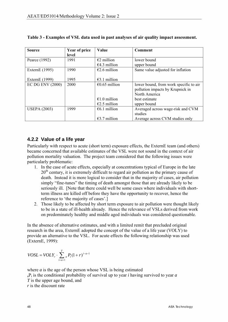
AEAT/ED51014/Methodology Volume 2: Issue 2
48 AEA Technology
Table 3 - Examples of VSL data used in past analyses of air quality impact assessment. Source Year of price
level Value Comment
Pearce (1992) 1991 �2 million �4.3 million
lower bound upper bound
ExternE (1995) ExternE (1999)
1990 1995
�2.6 million �3.1 million
Same value adjusted for inflation
EC DG ENV (2000) 2000 �0.65 million �1.0 million �2.5 million
lower bound, from work specific to air pollution impacts by Krupnick in North America best estimate upper bound
USEPA (2003) 1999 �6.1 million �3.7 million
Averaged across wage-risk and CVM studies Average across CVM studies only
4.2.2 Value of a life year Particularly with respect to acute (short term) exposure effects, the ExternE team (and others) became concerned that available estimates of the VSL were not sound in the context of air pollution mortality valuation. The project team considered that the following issues were particularly problematic:
1. In the case of acute effects, especially at concentrations typical of Europe in the late 20th century, it is extremely difficult to regard air pollution as the primary cause of death. Instead it is more logical to consider that in the majority of cases, air pollution simply �fine-tunes� the timing of death amongst those that are already likely to be seriously ill. [Note that there could well be some cases where individuals with short-term illness are killed off before they have the opportunity to recover, hence the reference to �the majority of cases�.]
2. Those likely to be affected by short term exposure to air pollution were thought likely to be in a state of ill-health already. Hence the relevance of VSLs derived from work on predominately healthy and middle aged individuals was considered questionable.
In the absence of alternative estimates, and with a limited remit that precluded original research in the area, ExternE adopted the concept of the value of a life year (VOLY) to provide an alternative to the VSL. For acute effects the following relationship was used (ExternE, 1999):
∑+=
−−+⋅=T
ai
aiiar rPVOLYVOSL
1
1)1(
where a is the age of the person whose VSL is being estimated aPi is the conditional probability of survival up to year i having survived to year a T is the upper age bound, and r is the discount rate
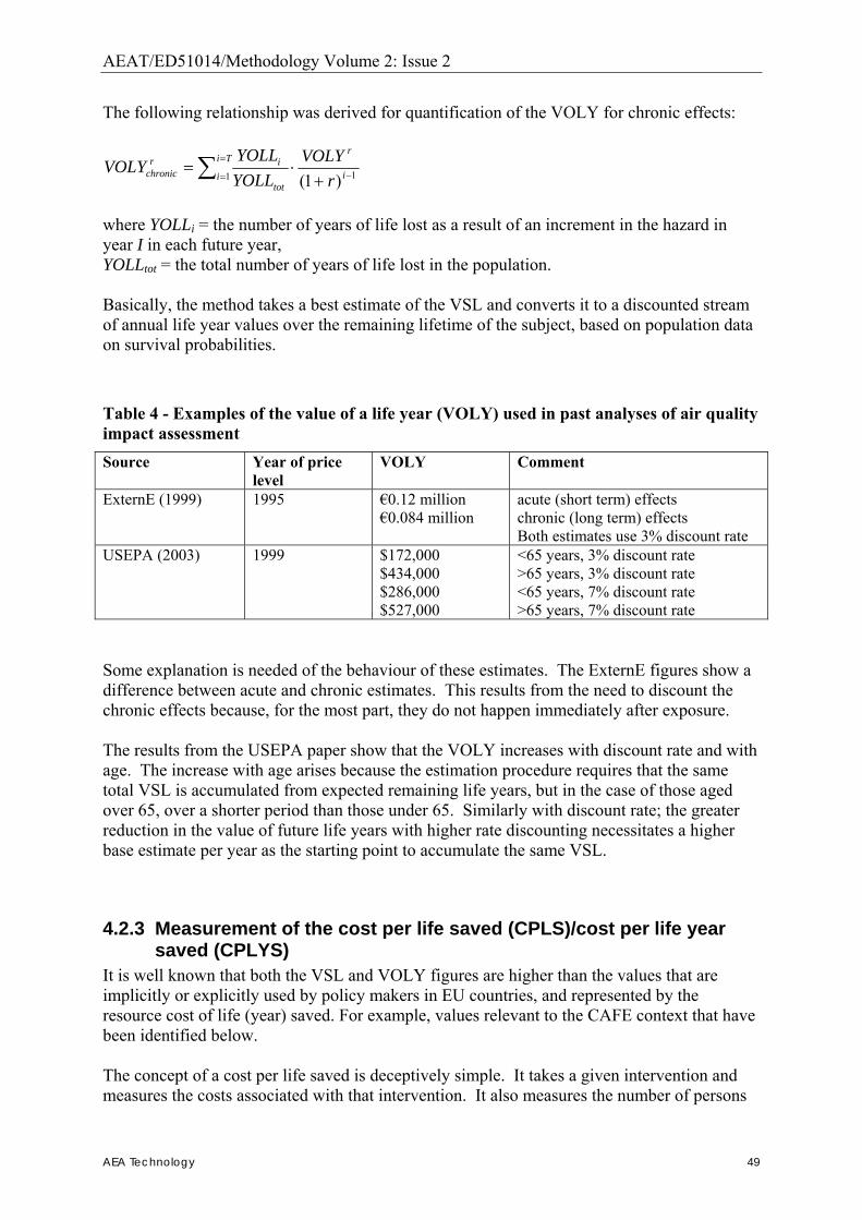
AEAT/ED51014/Methodology Volume 2: Issue 2
AEA Technology 49
The following relationship was derived for quantification of the VOLY for chronic effects:
11 )1( −
=
= +⋅= ∑ i
rTi
itot
irchronic r
VOLYYOLLYOLL
VOLY
where YOLLi = the number of years of life lost as a result of an increment in the hazard in year I in each future year, YOLLtot = the total number of years of life lost in the population. Basically, the method takes a best estimate of the VSL and converts it to a discounted stream of annual life year values over the remaining lifetime of the subject, based on population data on survival probabilities.
Table 4 - Examples of the value of a life year (VOLY) used in past analyses of air quality impact assessment Source Year of price
level VOLY Comment
ExternE (1999) 1995 �0.12 million �0.084 million
acute (short term) effects chronic (long term) effects Both estimates use 3% discount rate
USEPA (2003) 1999 $172,000 $434,000 $286,000 $527,000
<65 years, 3% discount rate >65 years, 3% discount rate <65 years, 7% discount rate >65 years, 7% discount rate
Some explanation is needed of the behaviour of these estimates. The ExternE figures show a difference between acute and chronic estimates. This results from the need to discount the chronic effects because, for the most part, they do not happen immediately after exposure. The results from the USEPA paper show that the VOLY increases with discount rate and with age. The increase with age arises because the estimation procedure requires that the same total VSL is accumulated from expected remaining life years, but in the case of those aged over 65, over a shorter period than those under 65. Similarly with discount rate; the greater reduction in the value of future life years with higher rate discounting necessitates a higher base estimate per year as the starting point to accumulate the same VSL.
4.2.3 Measurement of the cost per life saved (CPLS)/cost per life year saved (CPLYS)
It is well known that both the VSL and VOLY figures are higher than the values that are implicitly or explicitly used by policy makers in EU countries, and represented by the resource cost of life (year) saved. For example, values relevant to the CAFE context that have been identified below. The concept of a cost per life saved is deceptively simple. It takes a given intervention and measures the costs associated with that intervention. It also measures the number of persons
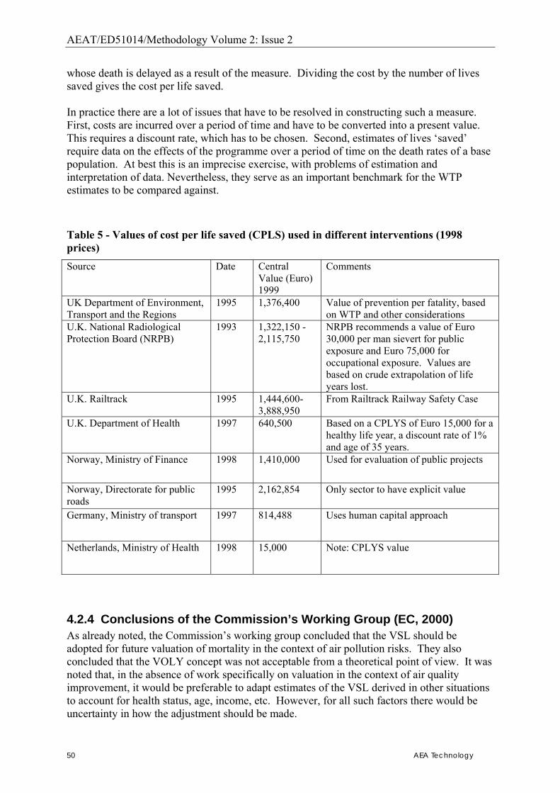
AEAT/ED51014/Methodology Volume 2: Issue 2
50 AEA Technology
whose death is delayed as a result of the measure. Dividing the cost by the number of lives saved gives the cost per life saved. In practice there are a lot of issues that have to be resolved in constructing such a measure. First, costs are incurred over a period of time and have to be converted into a present value. This requires a discount rate, which has to be chosen. Second, estimates of lives �saved� require data on the effects of the programme over a period of time on the death rates of a base population. At best this is an imprecise exercise, with problems of estimation and interpretation of data. Nevertheless, they serve as an important benchmark for the WTP estimates to be compared against.
Table 5 - Values of cost per life saved (CPLS) used in different interventions (1998 prices) Source Date Central
Value (Euro) 1999
Comments
UK Department of Environment, Transport and the Regions
1995 1,376,400 Value of prevention per fatality, based on WTP and other considerations
U.K. National Radiological Protection Board (NRPB)
1993 1,322,150 - 2,115,750
NRPB recommends a value of Euro 30,000 per man sievert for public exposure and Euro 75,000 for occupational exposure. Values are based on crude extrapolation of life years lost.
U.K. Railtrack 1995 1,444,600- 3,888,950
From Railtrack Railway Safety Case
U.K. Department of Health 1997 640,500 Based on a CPLYS of Euro 15,000 for a healthy life year, a discount rate of 1% and age of 35 years.
Norway, Ministry of Finance 1998 1,410,000 Used for evaluation of public projects
Norway, Directorate for public roads
1995 2,162,854 Only sector to have explicit value
Germany, Ministry of transport 1997 814,488 Uses human capital approach
Netherlands, Ministry of Health 1998 15,000 Note: CPLYS value
4.2.4 Conclusions of the Commission’s Working Group (EC, 2000) As already noted, the Commission�s working group concluded that the VSL should be adopted for future valuation of mortality in the context of air pollution risks. They also concluded that the VOLY concept was not acceptable from a theoretical point of view. It was noted that, in the absence of work specifically on valuation in the context of air quality improvement, it would be preferable to adapt estimates of the VSL derived in other situations to account for health status, age, income, etc. However, for all such factors there would be uncertainty in how the adjustment should be made.
AEAT/ED51014/Methodology Volume 2: Issue 2
AEA Technology 51
A major problem with the VOLY approach is that the value of statistical life is not linearly related to the loss of life years for individual mortality. If it were, one would expect the VSL to decline markedly with age. Some studies have reported a decline, but only by a relatively small amount (e.g. Jones-Lee (1985) who found a 30% decline over time: and Alberini et al (2004) who found in Canada a 25% decline after the age of 70, a significant effect, but one that is not in line with anticipated behaviour of the VSL according to the VOLY concept). Against this background it is interesting to note that the USEPA�s recent technical guidance in this area includes estimates based on both the VSL and VOLY concepts � with the VOLYs used in appraising the Clean Air Act being derived from VSL estimates using broadly the same approach as ExternE.
4.3. New empirical evidence As noted above, new studies are now appearing on mortality valuation that have sought to investigate the issue from the specific context of air pollution. The two studies of interest are the EC NewExt study and the UK DEFRA study and details of these are presented in the following sub-sections.
4.3.1 The NewExt study Method This study had as its objective the derivation of unit values to account in monetary terms for the incidence of premature death estimated to result from air pollution in Europe. Values were derived from three surveys undertaken simultaneously in UK, France and Italy, using a common survey instrument. The survey instrument adopted by the country teams in UK, France and Italy was developed using extensive face-to-face interviews in the USA, and was pre-tested in the USA, Japan and in Canada before being used for full sample surveys in these countries. It is self-administered and computerised. The survey protocol was to include those people over the age of 40, with one third of the sample being over the age of 60. The three EU country teams each conducted a series of focus groups and/or one-to-one testing in order to adapt the instrument for the national contexts. Additionally, the French country team tested a series of variants to the questionnaire on samples of about 50 each. The survey instrument is designed to elicit WTP for mortality risk reductions. Specifically, people were asked to value an immediate 5 in 1000 risk reduction, (the risk change being spread over the next ten years), an immediate 1 in 1000 risk reduction, and a reduction of 5 in 1000 to be experienced at age 70, in that order. (Wave 2 in the N. American studies reversed the order of the immediate risk changes). These changes are in the appropriate range for capturing the risk reductions associated with pollution reductions. The France study also implemented the Wave 2 design, whereby the 1 in 1000 risk reduction was valued first.
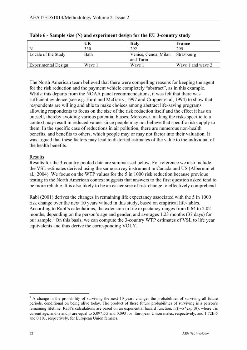
AEAT/ED51014/Methodology Volume 2: Issue 2
52 AEA Technology
Table 6 - Sample size (N) and experiment design for the EU 3-country study UK Italy France N 330 292 299 Locale of the Study Bath Venice, Genoa, Milan
and Turin Strasbourg
Experimental Design Wave 1 Wave 1 Wave 1 and wave 2 The North American team believed that there were compelling reasons for keeping the agent for the risk reduction and the payment vehicle completely �abstract�, as in this example. Whilst this departs from the NOAA panel recommendations, it was felt that there was sufficient evidence (see e.g. Hurd and McGarry, 1997 and Cropper et al, 1994) to show that respondents are willing and able to make choices among abstract life-saving programs allowing respondents to focus on the size of the risk reduction itself and the effect it has on oneself, thereby avoiding various potential biases. Moreover, making the risks specific to a context may result in reduced values since people may not believe that specific risks apply to them. In the specific case of reductions in air pollution, there are numerous non-health benefits, and benefits to others, which people may or may not factor into their valuation. It was argued that these factors may lead to distorted estimates of the value to the individual of the health benefits. Results Results for the 3-country pooled data are summarised below. For reference we also include the VSL estimates derived using the same survey instrument in Canada and US (Albernini et al., 2004). We focus on the WTP values for the 5 in 1000 risk reduction because previous testing in the North American context suggests that answers to the first question asked tend to be more reliable. It is also likely to be an easier size of risk change to effectively comprehend. Rabl (2001) derives the changes in remaining life expectancy associated with the 5 in 1000 risk change over the next 10 years valued in this study, based on empirical life-tables. According to Rabl�s calculations, the extension in life expectancy ranges from 0.64 to 2.02 months, depending on the person�s age and gender, and averages 1.23 months (37 days) for our sample.3 On this basis, we can compute the 3-country WTP estimates of VSL to life year equivalents and thus derive the corresponding VOLY.
3 A change in the probability of surviving the next 10 years changes the probabilities of surviving all future periods, conditional on being alive today. The product of these future probabilities of surviving is a person�s remaining lifetime. Rabl�s calculations are based on an exponential hazard function, h(t)=α*exp(βt), where t is current age, and α and β are equal to 5.09*E-5 and 0.093 for European Union males, respectively, and 1.72E-5 and 0.101, respectively, for European Union females.
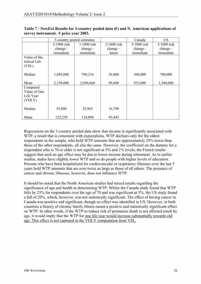
AEAT/ED51014/Methodology Volume 2: Issue 2
AEA Technology 53
Table 7 - NewExt Results for 3-country pooled data (�) and N. American applications of survey instrument. � price year 2003. 3-country pooled estimates Canada US 5:1000 risk
change - immediate
1:1000 risk change -
immediate
5:1000 risk change �
latent
5:1000 risk change -
immediate
5:1000 risk change -
immediate Value of Sta-tistical Life (VSL) Median Mean
1,045,000
2,150,000
788,216
2,956,668
36,800
99,600
506,000
933,000
700,000
1,540,000 Computed Value of One Life Year (VOLY) Median Mean
55,800
125,250
35,962
134,898
16,790
45,442
Regressions on the 3-country pooled data show that income is significantly associated with WTP, a result that is consistent with expectations. WTP declines only for the oldest respondents in the sample, who hold WTP amounts that are approximately 25% lower than those of the other respondents, all else the same. However, the coefficient on the dummy for a respondent who is 70 or older is not significant at 5% and 1% levels; the French results suggest that such an age effect may be due to lower income during retirement. As in earlier studies, males have slightly lower WTP and so do people with higher levels of education. Persons who have been hospitalized for cardiovascular or respiratory illnesses over the last 5 years hold WTP amounts that are over twice as large as those of all others. The presence of cancer and chronic illnesses, however, does not influence WTP. It should be noted that the North American studies had mixed results regarding the significance of age and health in determining WTP. Whilst the Canada study found that WTP falls by 25% for respondents over the age of 70 and was significant at 5%, the US study found a fall of 20%, which, however, was not statistically significant. The effect of having cancer in Canada was positive and significant, though no effect was identified in US. However, in both countries a history of chronic family illness meant a positive and statistically significant effect on WTP. In other words, if the WTP to reduce risk of premature death is not affected much by age, it would imply that the WTP for one life year would increase substantially towards old age. This effect is not captured in the VOLY computation from VSL.
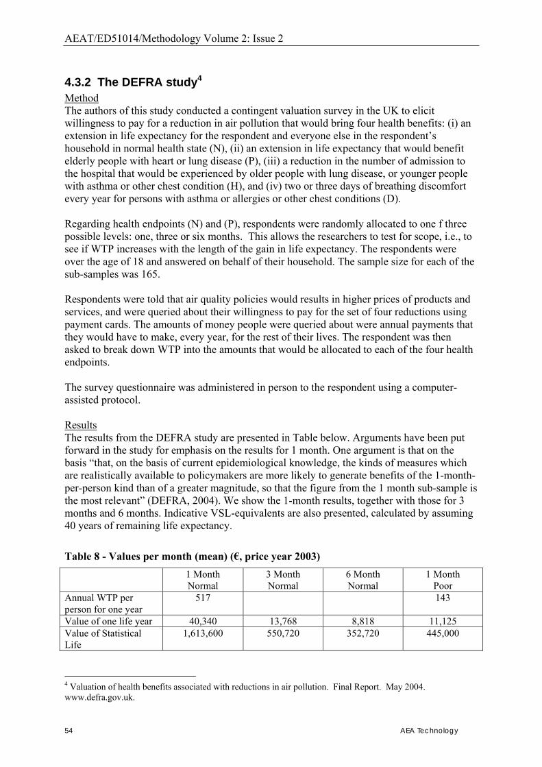
AEAT/ED51014/Methodology Volume 2: Issue 2
54 AEA Technology
4.3.2 The DEFRA study4 Method The authors of this study conducted a contingent valuation survey in the UK to elicit willingness to pay for a reduction in air pollution that would bring four health benefits: (i) an extension in life expectancy for the respondent and everyone else in the respondent�s household in normal health state (N), (ii) an extension in life expectancy that would benefit elderly people with heart or lung disease (P), (iii) a reduction in the number of admission to the hospital that would be experienced by older people with lung disease, or younger people with asthma or other chest condition (H), and (iv) two or three days of breathing discomfort every year for persons with asthma or allergies or other chest conditions (D). Regarding health endpoints (N) and (P), respondents were randomly allocated to one f three possible levels: one, three or six months. This allows the researchers to test for scope, i.e., to see if WTP increases with the length of the gain in life expectancy. The respondents were over the age of 18 and answered on behalf of their household. The sample size for each of the sub-samples was 165. Respondents were told that air quality policies would results in higher prices of products and services, and were queried about their willingness to pay for the set of four reductions using payment cards. The amounts of money people were queried about were annual payments that they would have to make, every year, for the rest of their lives. The respondent was then asked to break down WTP into the amounts that would be allocated to each of the four health endpoints. The survey questionnaire was administered in person to the respondent using a computer-assisted protocol. Results The results from the DEFRA study are presented in Table below. Arguments have been put forward in the study for emphasis on the results for 1 month. One argument is that on the basis �that, on the basis of current epidemiological knowledge, the kinds of measures which are realistically available to policymakers are more likely to generate benefits of the 1-month-per-person kind than of a greater magnitude, so that the figure from the 1 month sub-sample is the most relevant� (DEFRA, 2004). We show the 1-month results, together with those for 3 months and 6 months. Indicative VSL-equivalents are also presented, calculated by assuming 40 years of remaining life expectancy.
Table 8 - Values per month (mean) (�, price year 2003) 1 Month
Normal 3 Month Normal
6 Month Normal
1 Month Poor
Annual WTP per person for one year
517 143
Value of one life year 40,340 13,768 8,818 11,125 Value of Statistical Life
1,613,600 550,720 352,720 445,000
4 Valuation of health benefits associated with reductions in air pollution. Final Report. May 2004. www.defra.gov.uk.
AEAT/ED51014/Methodology Volume 2: Issue 2
AEA Technology 55
4.4. Summaryof values to be used in theCAFE CBA We will use the new studies for mortality valuation in CAFE, on the basis that, unlike previous work, both studies were designed specifically to measure the WTP for mortality changes associated with air pollution. In reaching our recommended values we will use of results from the NewExt work since they are more representative of the EU population: three EU Member States were surveyed and the total size for the 5:1000 immediate risk change question was 930, whilst the DEFRA study covers one country only and has a sample size of 165 for the 1 month life expectancy change. For recommendations relating to VOLY, however, it is important to point out that the DEFRA study directly values a change in life expectancy, while the NewExt work computed values of one life year from the values of statistical life. For chronic mortality for particulates (i.e. the results of the cohort studies), the new studies give specific empirical values for a year of life lost. We feel that it is appropriate to use this metric, as this is the preferred (central) approach from the health impact assessment analysis. However, because of the weaknesses of the VOLY approach � outlined above � we also quantify separately using the VSL, which has a strong empirical basis. We will use the results from the NewExt study which relate to WTP in normal health since the section on epidemiology above suggests that this is most appropriate to describing the chronic impact. The NewExt results (adjusted from price year 2003 to 2000 for consistency with RAINS) suggest central VOLY values of �52,000 (from the study median) and �120,000 (from the study mean). We also need to consider adjustment for the quality of the life lost. The NewExt study finds that the fact that a respondent has a chronic heart or lung condition does not influence WTP per se. However, those persons who have been hospitalized for cardiovascular or respiratory illnesses over the last 5 years have WTP amounts that are, everything else being the same, roughly twice as large as those of all others. Therefore, as a sensitivity we apply a multiplier of two Central VSL values are based on the NewExt study of �980,000 (from the study median) and �2 million (from the study mean), both expressed for price year 2000. WTP values from the 1 in 1000 risk change question, combined with the adjustment for health condition gives an upper bound sensitivity value of �5.6 million. For particulates (PM10/PM2.5) we do not propose to separately quantify impacts using the time-series studies for the main analysis. We believe to do so would be double counting. However, given the large amount of research on this end-point a quantification will be undertaken for purposes of illustration. We will value the effects of short-term exposure and mortality from ozone as part of the core analysis. The question of whether to use the VSL or VOLY approach for valuation is more problematic for dealing with the acute impacts of ozone. For these acute mortality effects of ozone (from the time-series studies), the health impact can best be characterised as �deaths brought forward� (generally by a short time compared to deaths from transport accidents). The time series studies provide results in terms of changes in the number of daily deaths associated with air pollution. Aggregated, these results can be represented as the number of deaths per annum whose immediate life shortening was attributable to air pollution in the days immediately preceding death. In at least some of these cases, the actual loss of life is likely to be small, though there is no direct evidence on the average loss of life.
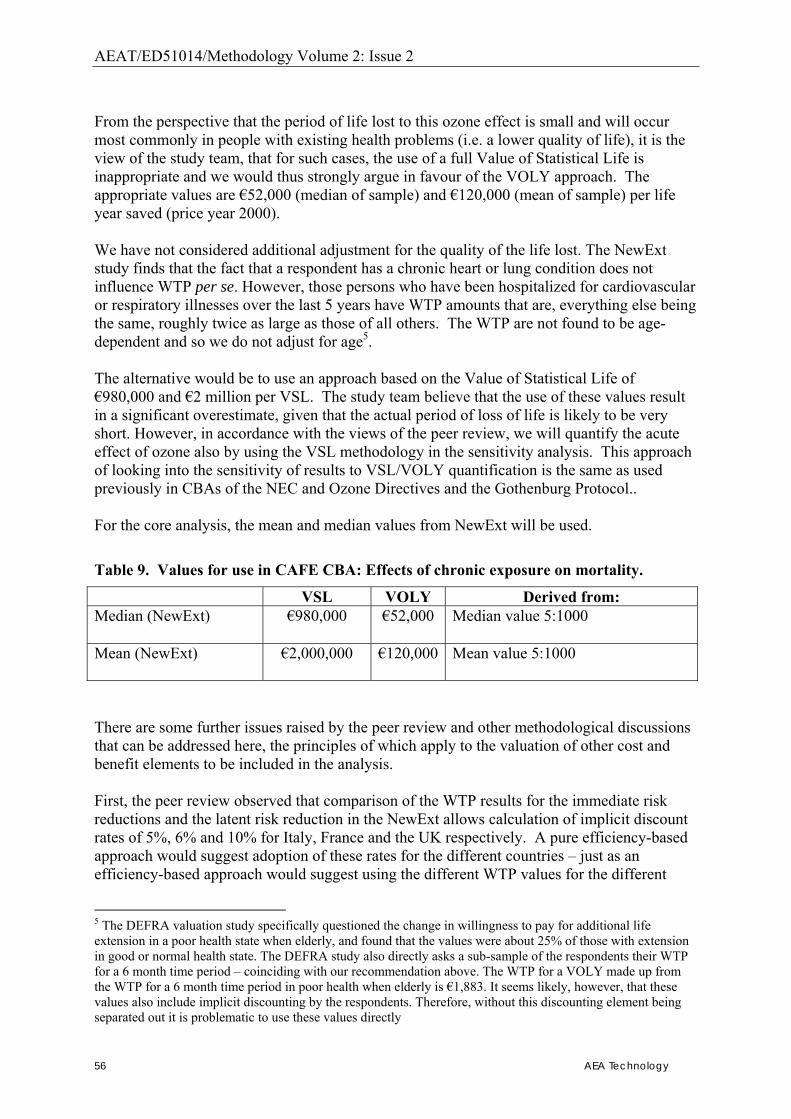
AEAT/ED51014/Methodology Volume 2: Issue 2
56 AEA Technology
From the perspective that the period of life lost to this ozone effect is small and will occur most commonly in people with existing health problems (i.e. a lower quality of life), it is the view of the study team, that for such cases, the use of a full Value of Statistical Life is inappropriate and we would thus strongly argue in favour of the VOLY approach. The appropriate values are �52,000 (median of sample) and �120,000 (mean of sample) per life year saved (price year 2000). We have not considered additional adjustment for the quality of the life lost. The NewExt study finds that the fact that a respondent has a chronic heart or lung condition does not influence WTP per se. However, those persons who have been hospitalized for cardiovascular or respiratory illnesses over the last 5 years have WTP amounts that are, everything else being the same, roughly twice as large as those of all others. The WTP are not found to be age-dependent and so we do not adjust for age5. The alternative would be to use an approach based on the Value of Statistical Life of �980,000 and �2 million per VSL. The study team believe that the use of these values result in a significant overestimate, given that the actual period of loss of life is likely to be very short. However, in accordance with the views of the peer review, we will quantify the acute effect of ozone also by using the VSL methodology in the sensitivity analysis. This approach of looking into the sensitivity of results to VSL/VOLY quantification is the same as used previously in CBAs of the NEC and Ozone Directives and the Gothenburg Protocol.. For the core analysis, the mean and median values from NewExt will be used.
Table 9. Values for use in CAFE CBA: Effects of chronic exposure on mortality.
VSL VOLY Derived from: Median (NewExt) �980,000
�52,000 Median value 5:1000
Mean (NewExt) �2,000,000
�120,000 Mean value 5:1000
There are some further issues raised by the peer review and other methodological discussions that can be addressed here, the principles of which apply to the valuation of other cost and benefit elements to be included in the analysis. First, the peer review observed that comparison of the WTP results for the immediate risk reductions and the latent risk reduction in the NewExt allows calculation of implicit discount rates of 5%, 6% and 10% for Italy, France and the UK respectively. A pure efficiency-based approach would suggest adoption of these rates for the different countries � just as an efficiency-based approach would suggest using the different WTP values for the different
5 The DEFRA valuation study specifically questioned the change in willingness to pay for additional life extension in a poor health state when elderly, and found that the values were about 25% of those with extension in good or normal health state. The DEFRA study also directly asks a sub-sample of the respondents their WTP for a 6 month time period � coinciding with our recommendation above. The WTP for a VOLY made up from the WTP for a 6 month time period in poor health when elderly is �1,883. It seems likely, however, that these values also include implicit discounting by the respondents. Therefore, without this discounting element being separated out it is problematic to use these values directly
AEAT/ED51014/Methodology Volume 2: Issue 2
AEA Technology 57
countries. For consistency with the discounting of other costs and benefits we prefer to adopt the common rates used in Commission�s impact assessment: of 4%- We will also calculate the sensitivities with 2% and 6% discount rates. Whilst the efficiency criterion alone suggests using different WTP values for different Member States, this has not been carried out by any analysis at European level. This is mainly because it would not be politically appropriate to use different values and also because there is also the practical challenge of getting such values from Member States. For instance, a WTP for increasing life expectancy has been derived only for a couple of Member States. Thus, also, data requirements would militate against pursuing a Member State by Member State approach. Finally, as the analysis is carried out at the EU level, it is justified to use the same average WTP values across all Member States. The peer review also commented that as incomes are expected to rise over time, so should the WTP valuations be expected to increase. At issue here is whether the two increase at the same rate. A number of studies have reported a positive relationship between income and WTP values, including the NewExt study, Hammitt and Liu (2004) etc. Whilst, we recognise this approach to be correct in itself, we are again constrained by the informational requirement that would arise were we to apply this mechanism across all costs and benefits (with potentially differing income elasticities). We will therefore adopt constant unit values across time. This is likely to result into some underestimation of benefits, as it is likely that the WTP increases when disposable income increases. Related to this, there is also an issue of discounting. Some of the benefits in life years will occur in the future (potentially over a much longer time frame than for the CAFE scenario), so it is important to consider the discounting of benefits, using a discount rate that is consistent with the other parts of the CAFE analysis (e.g. on costs) and, indeed, analysis for the European Commission more generally. This is a social rate of time preference of 4%6. For longer-term analysis (e.g. working with life table over a 75 � 100 year times-scale) a different approach is often taken in environmental cost-benefit analysis. This uses a pure rate of time preference (PRTP), for example of 1.5%7. The logic for this is that benefits, such as for example a change in the risk of death, might be seen as having a broadly constant utility value over time, regardless of changes in income. If so, then such future benefits can be valued in current values and discounted at [the pure time preference rate], so avoiding the need to calculate separately a rate of increase in their value over time. Within the first phase of the project, we have not discounted future life years lost (or gained), though the assumption of no lag phase reduces the importance of any discounting significantly. It will be considered in future revisions of the methodology. Given that no discounting of the benefits are undertaken, this is likely to lead to an over estimation of the benefits. Taking together the fact that WTP is likely to increase over time (either with the same rate as GDP or somewhat higher or lower) and the fact that future benefits are not discounted, an implicit � and most likely realistic � assumption in the methodology is that these two effects cancel each other out. A further sensitivity that could be examined concerns alternative assumptions on time-lags between changes in pollution and death rates. Most health impact assessments that use cohort 6 Related to the paragraph above, when considering a much longer time-frame, the effects of incomes rises over time, and WTP rises, are also relevant. 7 The value of a 1.5% PRTP is broadly consistent with the current EC recommended discount rate of 4% social rate of time preference (assuming average GDP per capita growth of 2.5%).

AEAT/ED51014/Methodology Volume 2: Issue 2
58 AEA Technology
studies assume no time-lag. This is the approach taken by RAINS and, for consistency, we will adopt this also for the main analyses for CAFE CBA. However, we will also carry out sensitivity analyses based on various assumed time-lags between changes in pollution and changes in death rates.
AEAT/ED51014/Methodology Volume 2: Issue 2
AEA Technology 59
5. Quantification of Mortality in Infants and Young Children There is now substantial evidence that higher air pollution is adversely associated with a wide range of measures of foetal and infant health, including mortality. The evidence on foetal health has been reviewed recently by Glinianaia et al. (2004a, b). Kaiser et al. (2004) also discuss the strength of evidence across a wide range of studies, in their assessment of the infant mortality attributable to air pollution in US metropolitan areas. The effects of air pollution on children�s health have been reviewed recently by the World Health Organisation. See http://www.euro.who.int/document/EEHC/execsum.pdf for the Executive Summary. In Europe the effects of air pollution on mortality and other indices of infant health have been studied most extensively by Bobak and co-workers, initially in the Czech Republic, but also more widely (Bobak and Leon 1992, 1999); Bobak (2000); Bobak et al. (2001). The most important endpoint, and the one most amenable to monetary valuation, is that of infant mortality.
5.1. Effects of chronic exposure on infant mortality
5.1.1 Available research In quantifying the benefits to health of the US Clean Air Act, it has been recommended that infant mortality be included and that quantification be based on the cohort study by Woodruff et al. (1997); Kaiser et al. (2004) based their risk assessment on the same study. Rabl (2003) uses results both from Woodruff et al. (1997) and from Bobak and Leon (1999). The associations reported by Woodruff et al. are with particulate matter, expressed as PM10 (mean outdoor concentrations of PM10 in the 1st two months of life) giving
Change in (all-cause) infant mortality of 4% per 10 µg/m3 PM10 (95% CI 2% - 7%)
Results were based on a study of 4 million infants, where post neonatal infant mortality was considered as death between the ages of one month and one year. Woodruff et al. report that infants� exposure to PM10 was positively associated with low maternal education, having unmarried parents and maternal smoking during pregnancy � all of these being variables that were adjusted for in the analysis. It is possible that exposure to PM10 was in addition associated with other, unmeasured, socio-economic confounding factors which, if not adjusted for, may have led to some over-estimation of the PM10-related coefficient. Kaiser et al. discuss in detail the many considerations involved in risk assessment of infant mortality, including their reasons for choosing Woodruff et al. (1997) as the main study on which to base quantification for the US, together with aspects of implementation. Drawing heavily on this discussion, we note a number of points relevant to CAFE CBA in the sections that follow.
AEAT/ED51014/Methodology Volume 2: Issue 2
60 AEA Technology
5.1.2 Use of cohort or of time series studies Most of the available studies are time series studies. Woodruff et al. is a cohort study and as such, we would expect that it captures more fully the effects of air pollution on mortality than time series studies could achieve. This is because time series studies detect the effects of recent exposures only (�daily variations�), whereas cohort studies capture effects arising from a full lifetime�s exposure. Note however that the estimated relative risks from time series studies are as high as, or higher than, those from the cohort study. This is contrary to the comparison of time series and cohort studies in adults. It is possible that this difference reflects regional differences � these time-series studies quoted by Kaiser et al. are all from non-European regions (Mexico, Latin America, East Asia), with different pollution and probably very different health status and health care of infants. It may however also reflect in part two aspects of study design that have been discussed much more extensively in relation to mortality in adults:
• It is possible that some aspects of time series studies are not captured fully by the cohort studies;
• The lifetime exposure that is captured by cohort studies is necessarily short � in the case of infants, the effective time-periods of time-series and of cohort studies are necessarily much more similar to one another than is the case with adults, and this may make it more likely that they give similar answers.
Thus, with infant mortality, there is a much stronger case for choosing the time series studies as an alternative to the cohort studies, and we will do this in some sensitivity analyses.
5.1.3 Frailty; study deaths (attributable cases) or life-years It is unclear to what extent the infant deaths associated with and presumably attributable to air pollution occur among young people who are already very frail, and so unlikely to survive into adulthood; and if so, to what extent air pollution (before birth as well as after) contributed to that frailty. This point is noted both by Kaiser et al. (2004) and in the US EPA discussions. The fact that the relative risk from time series studies is as high as, or higher than, the cohort study estimates does suggest that frailty is an issue. On that basis, Kaiser et al. proposed and carried out an assessment based on attributable cases (deaths) rather than on life-years. Their reasons seem valid and we will do the same for the core analyses of CAFE CBA. The difficulty of not knowing what is the real reduction in life expectancy is not however entirely by-passed. Rather it appears, at least implicitly, in judgements about what monetary valuation (VSL, VPF) should be ascribed to the attributable deaths. As noted earlier, Rabl (2003) argues that attributable cases cannot be estimated reliably in the context of air pollution. He uses life table methods to estimate the LY attributable to air pollution as a result of infant mortality. His analysis assumes a full life expectancy (i.e. about 77 years) associated with each infant death. We will carry out some corresponding life table analyses, to put infant morality in context of adult mortality. With the monetary valuation that will be applied, results using both methods will give similar answers. On that basis, we will carry out a core implementation in terms of attributable cases, without comment on the underlying �correctness� of using attributable cases or LY:
Population at risk x baseline death rate x .004 x change in µg/m3 PM10
AEAT/ED51014/Methodology Volume 2: Issue 2
AEA Technology 61
5.1.4 Cause-specific or all-cause mortality Using the coefficients of Woodruff et al., Kaiser et al. found that results (attributable cases) from quantifying all-cause mortality are similar to the aggregate results from cause-specific assessments for the US, involving sudden infant death (SID) syndrome and respiratory disease mortality, the latter contributing less to the overall impact compared to SID. This is reassuring as an aspect of coherence; however, no effect remained in the Bobak and Leon (1998) study after respiratory deaths were taken into account, which suggests that the findings for SID may have been different in the Czech study. Nevertheless, the impact assessment on all-cause mortality requires fewer and more accessible background data; HIA for adults is usually done on an all-cause rather than cause-specific basis, even though only some causes are affected; and so we think that an all-cause implementation for infants is justified also.
5.1.5 Which pollutant? Although relationships are expressed in relation to PM10, PM may to some extent be capturing some effects of the wider total air pollution mixture. If, on the other hand, the gases do play a part, it is likely that their effects are under-estimated.
5.1.6 Transferability; functions for an implementation in Europe Kaiser et al. note problems with transferability. In addition to the usual factors � e.g. differences in air pollution mixture � differences in factors such as access to and use of health services, and mother�s age at birth, are likely to be relevant and to vary geographically. These issues apply in CAFE CBA because a European-wide implementation will involve spatial extrapolation � transfer of relationships from US to Europe (if we use Woodruff et al.), or generalisation from some European countries to many (if we use Bobak and Leon). Rabl (2003) found that estimated impacts using all-cause infant mortality were similar regardless of whether impact estimation was based on coefficients taken from Woodruff et al. (1997) or from Bobak and Leon (1999). (Use of the latter required �conversion� from TSP to PM10). Furthermore, Rabl (2003) found that in terms of life-years � even when attributing a full life expectancy to each infant death � estimated impacts from infant mortality were but a small fraction of the impacts estimated from mortality in adults. Thus, while it is important to provide estimates that are realistic, it is not necessary to struggle particularly hard at choosing between two studies that give similar results.
5.1.7 Recommendation All things considered, we use Woodruff et al (1977). Based on available European studies, it is possible, perhaps even likely, that the relative risk is too small rather than too large. On the other hand it is unclear to what extent the earlier or extra infant deaths would have occurred in any case at a young age; and under these circumstances attributing a full VSL to the effects of air pollution is likely to over- rather than under-estimate the benefits of reducing air pollution. There is no good basis for saying that the �trade-off� between these two factors ensures a �correct� answer. We do, however, note and recognise that the implied bias works in opposite directions for impacts (possibly too low) and for valuation (possibly too high).
AEAT/ED51014/Methodology Volume 2: Issue 2
62 AEA Technology
5.2. Effects of acute exposure in children under five years; and, more generally, mortality effects (chronic and acute exposure) in people under 30 years of age
Most time series studies study people at all ages, i.e. the full population-at-risk in the location (usually a city) being studied. Accordingly, HIA of attributable cases based on time series studies usually refer to deaths at all ages. Note that we will not add estimates of PM-related mortality from time series studies to the estimates from cohort studies. This is to avoid double-counting. The �general� cohort studies however are studies of adults, at ages 30 or more (Pope et al., 2002) or 25 or more (Dockery et al., 1993). In order to avoid extrapolation, risk assessments based on these studies usually apply changes in death rates only to people in adulthood, e.g. at ages 30 or more; and this is what we also plan to do in our main analyses. This overall approach for PM and mortality (using results from and impacts based on the cohort studies; applying changes in death rates to people over 30 only; and not including in addition the effects as estimated from time series studies) means that PM-related mortality effects in people under 30 are not included in the assessments. The inclusion of pollution-related mortality effects for infants goes some way towards redressing this omission. It is likely that the remaining omission is not large relative to the effects that are quantified, because in Europe death rates at young age groups are generally low. Should and can more be done? We think yes, as sensitivity analyses. There are three main possibilities:
i. Extend implementation of the cohort studies to include deaths at younger ages also. As noted, this involves an extrapolation. The fact that causes of death are different in younger and in older people might caution against this. On the other hand, there is evidence from time series studies of effects at ages younger than 30 years. Also, the RR for infant mortality from Woodruff et al. (1997), of 1.04 per 10 µg/m3 PM10, is very similar to the RR of 1.06 per 10 µg/m3 PM2.5 estimated for adults by Pope et al. (2002) if, for example, we use the conversion factor of 0.6PM10=PM2.5, as proposed initially by Dockery and Pope (1994).
ii. Estimate effects at ages less than 30 based on time series studies and add to the cohort
study estimates. iii. Some time series studies show relative risks in children under 5 years of age that are
slightly higher than the effects at all ages as estimated in time series studies generally. It is possible to use these for quantification, though the specific studies � Kaiser et al. (2004) quote Ostro et al. (1999) and Conceicao et al. (2001) for studies in Bangkok and Sao Paolo respectively � may be unrepresentative for the situation in Europe generally.

AEAT/ED51014/Methodology Volume 2: Issue 2
AEA Technology 63
We will, in the course of the study, explore these options from the viewpoint of whether or not it matters to take account of PM-related mortality at younger ages; i.e. whether or not the estimated effects are large, compared with other uncertainties in the overall assessment. Preliminary work with life tables (strategy i. above) suggests that it makes little difference to estimated impacts, whether the changes in death rates are applied at all ages or only at age 30 or more. This supports the view that the omission is not very important practically.

AEAT/ED51014/Methodology Volume 2: Issue 2
64 AEA Technology
6. Valuation of Mortality in Infants and Young Children
6.1. Introduction There is a paucity of research in this area, and the conflicting results from the limited existing literature leaves little guidance for policy makers on how to value health risks to children. For example, due to the lack of empirical research on VSL, most economic analyses rely on adult VSL for children�s health effects. Indeed, in the United States EPA�s �Children�s Health Valuation Handbook� recommends that �with few child health valuation studies available, analysts may need to rely on transferring adult benefits to children until more information becomes available� (US EPA 2003, pp. 1-6). In the following paragraphs we review the evidence that can be considered in the context of CAFE and make some suggestions as to what values can be used in the first instance.
6.2. Methodological issues A number of methodological and empirical issues must be resolved. The first methodological issue is which perspective to adopt. Generally, economists prefer to derive WTP values for health risk reductions from the willingness of individuals to pay for risk reductions that affect themselves. This approach would clearly present difficulties in the case of children, as children have neither the maturity nor the financial resources to clearly define their willingness-to-pay. In short, the basic tenets of welfare economics cannot reasonably be assumed to represent children. Therefore, an alternative perspective has to be adopted from which to estimate child health values. There are three potential perspectives from which preferences for children�s health risks might be elicited: (i) that of society (parents and non-parents), (ii) that of adults placing themselves in the position of children, and (iii) that of parents assessing risks faced by their own children (Dockins et al. 2002). Obtaining a societal WTP presents problems of double-counting due to altruism (Jones-Lee 1991; Jones-Lee 1992). The parental perspective has the advantage that literature is available, albeit sparse. We report on this literature below. Other methodological issues that make transfer of values from adults to children difficult include:
• Differences in the nature and/or extent of impact risks. There is, for example, considerable uncertainty in the epidemiological literature as to the likelihood and magnitude of health impacts on children (Tamburlini, 2003).
• The potential importance of altruism. This is clearly important when parents assess their children�s health risks though the identification of the type of altruism involved in determining WTP is difficult.
• The relationship between WTP and age. This is important for example when a measure of life years is used in the valuation � particularly when the child�s life expectancy is uncertain.
• Household composition and structure. Within the parental perspective approach it is likely that the nature of the household formation will influence WTP. For example,
AEAT/ED51014/Methodology Volume 2: Issue 2
AEA Technology 65
WTP has been found in some studies to be less for children in larger families, and for single parent families to be WTP more for avoiding illness in their child than dual parent families.
• Discounting. Subjective discount rates may be different for adults and their own WTP compared to those for their children.
6.3. Empirical issues A number of studies have examined possible differences of values between adults and children, but their findings have been mixed. The majority of studies find that the value of children�s health benefits is higher than those of adults (Lewis and Charney, 1989; Busschbach et al., 1993; Cropper et al., 1994; Liu et al., 2000; Dickie and Ulery, 2001). However, other research has generated estimates of WTP for child and adult health that are similar (Blomquist, 2003; Mount et al., 2001) and one study estimates the value of statistical life for a child that is lower than the value of a statistical adults life (Jenkins et al. 2001). The findings of these studies that are of most relevance in the context of valuing the avoidance of children�s premature death are presented in the table below. It should be emphasized that none of the above listed studies consider the EU context and that there are many questions and obstacles surrounding the validity of transferring mortality risk values across countries (Pearce 2000). Nevertheless, some conclusions can be drawn at this stage.
• Parents are more willing to pay to reduce their children�s health risks than their own. The estimated marginal rate of substitution (MRS) is generally greater than one, and is typically about 2.
• Values for younger children are generally found to be higher than for older children. • Values for the reduction of children�s mortality risk are greater than the values for
the reduction of morbidity risk. This is consistent with the WTP values for adults and is consistent with economic theory.
The methodological difficulties outlined above that remain unresolved � combined with the differences between studies and the spatial and temporal transfer issues - make it very difficult to transfer these results to our current context with any great confidence.
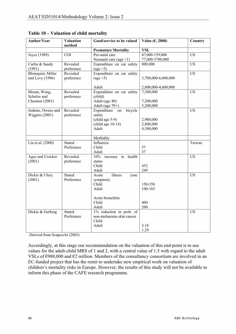
AEAT/ED51014/Methodology Volume 2: Issue 2
66 AEA Technology
Table 10 � Valuation of child mortality Author/Year Valuation
method Good/service to be valued Value (�, 2000) Country
Premature Mortality VSL Joyce (1989) COI Pre-natal care
Neonatal care (age <1) 47,000-159,000 77,000-3700,000
US
Carlin & Sandy (1991)
Revealed preference
Expenditure on car safety (age <5)
800,000 US
Blomquist, Miller and Levy (1996)
Revealed preference
Expenditure on car safety (age <5) Adult
3,700,000-6,000,000 2,800,000-4,600,000
US
Mount, Weng, Schulze and Chestnut (2001)
Revealed preference
Expenditure on car safety (child) Adult (age 40) Adult (age 70+)
7,300,000 7,200,000 5,200,000
US
Jenkins, Owens and Wiggins (2001)
Revealed preference
Expenditure on bicycle safety (child age 5-9) (child age 10-14) Adult
2,900,000 2,800,000 4,300,000
US
Morbidity Liu et al. (2000) Stated
Preference Influenza Child Adult
57 37
Taiwan
Agee and Crocker (2001)
Revealed preference
10% increase in health status Child Adult
452 249
US
Dickie & Ulery (2001)
Stated Preference
Acute illness (one symptom): Child Adult Acute bronchitis Child Adult
150-350 100-165 400 200
US
Dickie & Gerking Stated Preference
1% reduction in prob. of non-melanoma skin cancer Child Adult
3.18 1.29
US
Derived from Scapecchi (2003) Accordingly, at this stage our recommendation on the valuation of this end-point is to use values for the adult-child MRS of 1 and 2, with a central value of 1.5 with regard to the adult VSLs of �980,000 and �2 million. Members of the consultancy consortium are involved in an EC-funded project that has the remit to undertake new empirical work on valuation of children�s mortality risks in Europe. However, the results of this study will not be available to inform this phase of the CAFE research programme.
AEAT/ED51014/Methodology Volume 2: Issue 2
AEA Technology 67
7. Quantification of Morbidity
7.1. Morbidity – Methodology; Limited use of impact functions
7.1.1 Basic approach The basic approach to estimating the effects of air pollution on human morbidity is similar to what is done for �acute� mortality; i.e. use a concentration-response (C-R) function expressed as
i. % change in endpoint (RR of new or �extra� cases, events or days) per (10) µg/m3
PM10 or ozone; link this with:
ii. the background rates of the endpoint (new cases, events or days per year per unit population � say, per 100,000 people) in the target population
iii. the population size iv. the relevant pollution increment, expressed in µg/m3 PM10 or ozone
and express the result as estimated new or �extra� cases, events or days per year.
7.1.2 Impact functions Note that the C-R function and background rates can be combined into a single impact function expressed as:
number of (new) cases, events or days per unit population (say, per 100,000 people) per (10) µg/m3 PM10 or ozone per annum
This impact function can then be linked, as before, with population size and the relevant pollution increment to give estimated impacts. This approach is most reliable when the impact function (i.e. the combination of C-R function and baseline rate) is reasonably stable spatially. However, we also use it as a means of enabling quantification when country �specific background rates are unavailable. Dealing with missing data on background rates For many health endpoints, data on background rates of morbidity are not collected routinely throughout Europe, or in practice the data that are collected routinely are very difficult (too resource-intensive) to collate. One approach is not to attempt quantification. As noted earlier, failure to quantify biases the analysis to under-estimate health effects. Another strategy is to use other general epidemiological studies of that health endpoint � not necessarily studies of air pollution and health � to provide estimates of background rates. Thus, for example, in the present evaluation we use results from the European Community Respiratory Health Study (ECRHS) of adults, and from the International Study of Asthma and Allergies in Children (ISAAC) to provide background data for various respiratory endpoints.
AEAT/ED51014/Methodology Volume 2: Issue 2
68 AEA Technology
A third strategy is to:
• estimate an impact function from where the relevant epidemiological studies were carried out; and
• transfer and use that impact function for quantification in the target population. There are, necessarily, issues about the transferability of such an impact function. The approach is, however, well established in HIA practice (see e.g. ExternE; Künzli et al., 2000). In CAFE CBA we will use all of these approaches as need dictates, sometimes checking that alternative strategies give estimates that are at least broadly consistent with one another. All of the impact pathways considered in the present report are of interest and are relevant to the health of people in Europe. However, as noted in earlier drafts, some pathways have a much greater impact than others on final estimates of monetised benefits. Even a relatively crude quantification can help identify which pathways are the most influential, so that efforts at improving the estimates can be focussed on those pollutant-endpoint combinations which, when combined also with valuation, have greatest impact on the final figures.

AEAT/ED51014/Methodology Volume 2: Issue 2
AEA Technology 69
8. MORBIDITY FROM CHRONIC EXPOSURE: PARTICULATE MATTER
8.1. The evidence The evidence has been reviewed by WHO for CAFE � particulate matter, Question 2 (http://www.euro.who.int/document/e79097.pdf). There are studies relating long-term exposure to PM to the health of children as expressed via reductions in lung function (FEV1, FVC) and symptoms of bronchitis (also sinusitis and frequent colds). In addition, other conditions (wheeze, conjunctivitis) are associated with pollution mixtures which include ambient PM, though where the role of PM has not been identified clearly Studies in adults have shown relationships with chronic cough, chronic phlegm and breathlessness; and with reductions in lung function.
8.2. Priorities for quantification There are two additional important additional considerations in using this evidence for quantification. First, it is more appropriate to quantify the effects of air pollution on new cases (incidence) than on prevalence of chronic disease, because a quantification of new cases (per year) relates better to the need in CBA to express results in terms of benefits per year. Second, we do not, currently, have suitable valuation data on lung function changes. A possibility is that this information gap might be tackled indirectly, by converting lung function changes to approximate equivalent risks of some established health entities such as chronic obstructive pulmonary disease (COPD), chronic symptoms and/or reduced life expectancy. Methods for doing this are not well-established at this point, and may be a development priority for HIA work. (Even though COPD is defined in terms of reduced lung function, usually as a joint reduction in FEV1 and in the ratio FEV1/ FVC, it is by no means straightforward to estimate equivalent cases of COPD from a study of lung function.) The priority for quantification within CAFE CBA is where data are available from longitudinal studies, allowing estimates of incidence, for endpoints other than lung function.
8.3. New cases of chronic bronchitis, in adults The US Seventh Day Adventist Study (the AHSMOG �Adventist Health Smog � study) is, we think, the only major study to date to quantify the effects of PM on the development (i.e. increase in new cases) of chronic bronchitis. Various modern HIAs use results from a series of AHSMOG study papers to provide C-R functions and baseline rates for quantification. We follow the approach of ExternE (1999) (see also Hurley et al., 2000), which uses a C-R function in the metric of PM10, based on Abbey at al. (1995a), with background incidence rates from Abbey et al. (1993), though refined to take account of remission rates, as estimated
AEAT/ED51014/Methodology Volume 2: Issue 2
70 AEA Technology
from Abbey et al. (1995a). This approach to baseline rates follows that used by the US EPA (Abt Associates, 2003). However, the US EPA (Blueprint for Clean Air Act Benefits Analysis) proposes an E-R function from Abbey et al. (1995b), in the metric of PM2.5. Künzli et al. (2000) used Abbey et al. (1993) both for C-R function (in the metric of TSP) and for background rates of incidence. The various approaches follow the relevant underlying papers in having different strengths and weaknesses. For example, results for PM2.5 in Abbey et al. (1995b) are based on a smaller set of data, but include more intensive reporting of statistical modelling, than those in Abbey et al. (1995a). On the other hand, results in the metric of PM2.5 are appropriate to the pollution modelling in CAFE CBA. We consider to what extent the different approaches give different answers and if these differences matter for the final estimates of CAFE CBA.
8.3.1 Choice of endpoint – new cases of ‘chronic bronchitis’ The AHSMOG study examined people on two occasions, about ten years apart � in 1977, and again in 1987/88. The adults studied were aged 27 years or more at enrolment in 1977. Chronic bronchitis was defined as reporting at survey the symptoms of chronic cough or sputum, on most days, for at least three months of the year, for at least two years. This is a milder definition than is used in many other studies, which require chronic cough and sputum on all days for at least three months of the year. New cases of chronic bronchitis were defined as those who met the criteria in 1987/88, but not in 1977, whereas remission cases met the criteria in 1977, but not 10 years later. It is likely that, as well as real changes in health, the reasons for �remission� include chance or changes in uncontrolled factors influencing response.
8.3.2 Background rate There were 234 new cases of definite chronic bronchitis symptoms in the 10-year period (i.e. in 1987 compared with 1977), out of 3310 who were not classified as having chronic bronchitis at the start � an attack rate of 0.707% (i.e. about 7 per 1000 at risk) annually over the 10-year period (Abbey et al., 1993, Table 3). This is the rate used by ExternE. The US EPA uses this crude incidence rate adjusted for remission. The rate of remission has been estimated at 46.6% (Abt Associates, 2003), using data from Table 1 of Abbey et al. (1995a). This gives a net incidence rate of
0.00707 (1-0.466); i.e. 0.378%, or 3.78 new cases annually per 1000 adults at risk It is unclear whether or not it is best to use the crude incidence rate or the rate adjusted for remissions in the present analysis. The European Lung White Book (2003) summarises experience in Europe, focussing on COPD, the nearest equivalent to chronic bronchitis as defined in AHSMOG. It reports that Krzyzanowski et al. (1986) found an annual attack rate of COPD of about 0.5% in a 13-year follow-up of adults aged 19-70 years in Krakow, Poland. Much more recently, Eagan et al. (2002, data derived from Table 3) reported a crude annual incidence rate for chronic cough of 0.82 in a general population study of 2819 adults aged 15-70 years, in Western Norway.
AEAT/ED51014/Methodology Volume 2: Issue 2
AEA Technology 71
On the other hand, the Global Burden of Disease project of WHO and the World Bank gives much lower figures for incidence of COPD in Europe. We derive approximate incidence rates in the population over 30 � this corresponds best to Abbey et al., and COPD is rare in people under 30 � by assuming that all new cases are in that age-group. Results, from GBD for the year 2000 (WHO, 2002), are given for three European Sub-Regions, classified by increasing rates of infant mortality, as follows:
• EuroA (Western Europe plus Croatia, Czech Republic, Israel, Slovenia): o incidence 479,000 new cases; o population 30+ is 261.602 million; o incidence rate among 30+ is 183 per 100,000
• EuroB (Most of Eastern Europe, but none of the EU25):
o incidence 110,000; o population 30+ 103.589 million o incidence rate among 30+ is 106 per 100,000
• Euro C (Nine Eastern European countries including Estonia, Hungary, Latvia,
Lithuania): o incidence 204,000; o population 30+ is 142.477 million o incidence rate among 30+ is 197 per 100,000
Overall incidence among adults 30+ is 156 per 100,000. On balance, it does seem more correct theoretically to use the net incidence rate, as providing a better estimate of the real underlying rate of development of chronic (i.e. lasting) respiratory disease; use of the higher figure would be difficult to justify, given the GBD results for incidence of COPD in Europe, although some commentators consider that the GBD estimates of COPD are low. Also, using the higher (unadjusted) rate, we have noted (e.g. ExternE, 1999; Hurley et al., 2000) that the estimated effects of PM on new cases of chronic bronchitis are high, and that the health endpoint being assessed is mild compared with other definitions of chronic bronchitis, including those that relate to the valuation studies. For CAFE CBA we will use the adjusted (i.e. lower) incidence rate for the main analyses, and the unadjusted to give a �high� value for sensitivity analyses only.
8.3.3 C-R function in metric of PM10, from Abbey et al. (1995a) Abbey et al., (1995a) is a longitudinal study of 3914 adults. It examines new cases of chronic bronchitis over a 10-year period: 1977 - 87/88, in relation to air pollution and other factors. Statistical analysis used logistic regression methods. The pollution exposure data included estimates of lifetime exposure to PM10, derived from TSP data. Analyses adjusted for covariates such as age, gender, education; and for respiratory symptoms in 1977 � this may imply over-adjustment for the effects of PM. These analyses led to an estimated RR of 1.15 per 20 µg/m3 PM10 (Table 6 of Abbey et al., 1995a). The result was not statistically significant at the 5% level, and a 95% CI is not given. However, there seems to be a consistency in these data, suggesting effects that are close to statistical significance at the 5% level. Thus, analyses using a different index (average annual
AEAT/ED51014/Methodology Volume 2: Issue 2
72 AEA Technology
hours spent in excess of 100µg/m3 PM10) reported a RR of 1.17 (95% CI 1.01, 1.35). Following ExternE (1999), we �adopt� the implied SE of 0.07352 and apply it to the designated RR of 1.15. This gives a CI of (0.99, 1.33), i.e. close to statistical significance, which seems plausible. Because the background incidence rate of 0.378% is so small, the logistic RR can be expressed as a % change, giving an estimate of
7.0% (95% CI -0.5%, 14.3%) change in baseline attack rates, per 10 µg/m3 PM10
8.3.4 Impact function in metric of PM10, from Abbey et al. (1995a) We link the C-R function with background rates (adjusted for remission) to find:
New cases of chronic bronchitis per year per 100,000 adults aged 27+ = background incidence rate (0.378%) × change per 10 µg/m3 PM10 (7%)
= 26.5 (95%CI -1.9, 54.1) per 10 µg/m3 PM10
8.3.5 C-R function in metric of PM2.5, from Abbey et al. (1995b) Estimates of ambient PM2.5 were derived using airport visibility data from nine airports scattered throughout California. The study was based on a subset of 1868 of the 3914 adults studied in Abbey et al. (1995a), selected because they lived for at least 80% of the period 1966-86 near one of those nine airports. Survey methods, and the definition of chronic bronchitis, were the same as before; there were 117 new cases over the 10-year period, from a possible 1748 subjects. Results (Abbey et al. 1995b, Table 2) showed an estimated RR of 1.81 (95% CI 0.98, 3.25) for a pollution increment of 45 µg/m3 PM2.5, or a relative risk of
1.141 (95% CI 0.996, 1.30%) per 10 µg/m3 PM2.5
Because this relative risk is to be applied to a background rate of new cases of bronchitis which is low, so that the odds of a new case are almost identical to the probability, then these relative risks are equivalent to percentage changes of
14.1% (95% CI -0.44%, 30.0%) per 10 µg/m3 PM2.5 Note that this is a high % increase � the highest of all those considered in the core analyses of this Report.
8.3.6 Impact function Linking the estimated RR and the adjusted or �net� background incidence rates of 0.378% per annum derived from Abbey et al. (1993) gives an estimated impact function as follows:
New cases of chronic bronchitis per year per 100,000 adults aged 27+ = background incidence rate (0.378%) × change per 10 µg/m3 PM10 (14.1%)
= 53.3 (95%CI -1.7, 113.4) per 10 µg/m3 PM2.5
AEAT/ED51014/Methodology Volume 2: Issue 2
AEA Technology 73
8.3.7 Preferred impact function Both impact functions have there strengths and weakness. Neither is statistically significant at the conventional 5% limit. While the impact function in PM2.5 is reported as being almost statistically significant, and results are not given for that in PM10, it is reasonable to infer that the function in PM10 was close to statistically significance also, and to derive a CI accordingly. The metric of PM2.5 is more appropriate to the present analysis. However, the % increase per 10 µg/m3 PM2.5 is very high. This is not to say that it is wrong � recent studies of mortality and long-term exposure to PM suggest that where PM is well differentiated spatially, as it is here, then estimated RRs can be high. On the other hand, we use a background incidence rate of 3.78 new cases per year per 100,000 adults at risk, i.e. higher than the incidence for Europe as estimated by the GBD project. In order to reduce the risk of accumulating an estimated impact that is too high, we choose
• The lower impact function of 26.5 (95%CI -1.9, 54.1) per 10 µg/m3 PM10 as core; • The higher impact function of 53.3 (95%CI -1.7, 113.4) per 10 µg/m3 PM2.5 for
sensitivity analyses. Population to which these impact functions should be applied The relevant population-at-risk is the population of all adults, aged 27 years or more, who do not have chronic bronchitis. The European Lung White Book reports that 4-6% of adults have clinically relevant COPD, so it may be that up to 95% of the adult population is at risk � this estimate may be a little on the high side.
8.3.8 Comments on reliability There is a broad consistency across the findings of this major study � results from several different papers, estimating exposures to PM in a wide variety of different ways, are broadly consistent with one another. Also, it has been possible to get some insights into the relevance to European conditions of the baseline (adjusted for remission) annual attack rate of the AHSMOG study, and to confirm that that rate is plausible. Note, however, that:
• Whichever paper is used to derive the C-R function, the result is based on one study only (AHSMOG), although other (cross-sectional) studies, and the literature as a whole provide strong supporting evidence of an effect;
• There are issues of transferability which are greater than those for chronic mortality � the AHSMOG study is not only US-based, but it refers to one part of the USA (California), and to a population of distinctive lifestyle;
• While many of the E-R relationships reported by Abbey et al. (1995a) are statistically significant, these were for effects above given exposure limits; the selected E-R functions, based on mean concentrations of PM10 or PM2.5, were not statistically significant at the 5% level.

AEAT/ED51014/Methodology Volume 2: Issue 2
74 AEA Technology
9. MORBIDITY FROM CHRONIC EXPOSURE: OZONE
9.1. The evidence The WHO for CAFE � ozone, Question 2 � highlights effects on lung function, on symptoms of bronchitis, on incidence of asthma and (in males only) on lung cancer effects. The larger and more representative ACS study (Pope et al., 2002) did not find a relationship between ozone and lung cancer mortality so we do not propose to quantify that endpoint. As for particles, our priority for quantification is in longitudinal studies of effects other than lung function.
9.2. Incidence of doctor-diagnosed asthma in adult men McDonnell et al. (1999) found a statistically significant relationship between reports of doctor-diagnosed asthma and long-term (20-year) concentrations of ambient ozone (mean 8-hr daily average), when investigating essentially the same cohort from the AHSMOG study as was studied by Abbey et al. (1995a). As for lung cancer, the relationship was found in men but not in women � possibly, the WHO review notes, because males spent more time outdoors. The relationship was robust to adjustment for other pollutants. The impact function can be derived from the relative risk and background rate: Relative risk Using logistic regression analyses, McDonnell et al. found a relative risk of
RR = 2.09 (95% CI 1.03-4.18) per 54 µg/m3 O3
Background rate Again from McDonnell et al., and following US EPA,
annual rate of asthma incidence = 2.19 per 1000 people at risk Applicable population
Adult men (aged 25+ or 27+) without asthma Applicable ozone concentrations
(8-hr daily max minus 35 ppb) averaged over days when 8-hr daily max exceeds 35 ppb Comments
• It is well-established that daily variations in air pollution cause exacerbations of asthma. The literature overall is however much more ambiguous about whether air pollution is a cause of new occurrences (incidence) of asthma, as was studied here.
• In addition the WHO review notes some methodological limitations of McDonnell et al., including that �low quality of outcome diagnosis might not allow a clear distinction between incidence and exacerbation�.

AEAT/ED51014/Methodology Volume 2: Issue 2
AEA Technology 75
• Finally, it is unclear to what extent and in what way the application of a cut-off point, designed for studies of daily variations, might affect the exposure-response relationship.
• For these reasons we propose not to quantify for this endpoint, a position consistent with the recommendations of Ostro in the peer review.
AEAT/ED51014/Methodology Volume 2: Issue 2
76 AEA Technology
10. MORBIDITY FROM ACUTE EXPOSURES: PARTICULATE MATTER AND OZONE
10.1. Hospital admissions
10.1.1 Introductory remarks There are numerous well-conducted studies, in Europe, North America and elsewhere, linking daily variations in air pollution with the numbers of people admitted to hospital on the same day, or on days immediately following. Before considering specific C-R functions, we make five general points:
i. Studies have examined the effect of air pollution on admissions to hospital for a wide range of respiratory (e.g. COPD, asthma, pneumonia, all respiratory) and cardiovascular (e.g. ischaemic heart disease (IHD), cerebrovascular, all cardiovascular) causes. In estimating impacts of air pollution on hospital admissions it is sufficient, simpler, and arguably better, to work with broad groupings such as �all respiratory� rather than to estimate effects separately by sub-cause, and then to aggregate, and we will seek to follow that simpler approach.
ii. Some studies, particularly in North America, have examined relationships only in elderly people, e.g. at age 65 years or more. This is principally for ease of study, not because the effects of air pollution are limited to the elderly � there are sufficient studies that show effects at other age groups also, despite lower rates of admissions. For that reason we will aim to provide C-R functions at all ages.
iii. Using all-age functions and wide cause groups should give estimates of total numbers which are as reliable as, or maybe more reliable than, a more disaggregated analysis. They will not however give such an accurate estimate of the age-distribution of the pollution-attributable cases, and a more disaggregated analysis would be needed if, e.g. monetary valuation varied by age or by detailed cause group.
iv. Many studies of hospital admissions and air pollution are based on general hospital admissions, i.e. both planned admissions and emergency admissions. It is to be expected, however, that daily variations in air pollution will impact on emergency admissions rather than on planned admissions. We plan therefore to use baseline data from emergency admissions only, if suitable data can be found.
v. Finally, it is unclear to what extent these �extra� hospital admissions in the days immediately following higher air pollution are genuinely extra new and additional admissions, or to what extent they reflect a �bringing forward� (by days or weeks or months) of events that would have occurred anyway (COMEAP, 1998). This is, in effect, the counterpart for hospital admissions of the �harvesting� issue often discussed with regard to daily variations in pollution and mortality. It is conventional to treat the attributable admissions as if they were genuinely new, and we follow that convention.

AEAT/ED51014/Methodology Volume 2: Issue 2
AEA Technology 77
10.1.2 Cardiovascular hospital admissions – in practice, cardiac hospital admissions (CHA, ICD 390-429)
Particulate matter (PM) WHO meta-analysis: The WHO meta-analysis identified studies in only two European cities � London and Edinburgh � with cardiovascular admissions (in the elderly, i.e. at 65+) as endpoint. It noted however that: • There is stronger evidence that daily variations in PM are related to cardiac admissions
(i.e. those affecting arteries near the heart itself) than to cerebrovascular admissions (stroke etc.) or to cardiovascular admissions generally;
• Le Tertre et al. (2002) provide a suitable C-R function for cardiac admissions from eight European cities in APHEA 2;
• Cardiac admissions may therefore be the more appropriate endpoint for quantification. We proceed with a quantification of cardiac admissions, basing our approach strongly on that used in the APHEIS study of cities in Europe. Apheis 2: The effects of daily variations of PM air pollution on cardiac admissions at all ages were studied and quantified in the Apheis 2nd report (Apheis-2). Figure 6 of Apheis-2 gave background rates of cardiac admissions at all ages from eight cities with emergency admissions and a further four cities with general admissions � it was not possible to get separate data on emergency admissions for these four cities. Apheis 3: C-R functions Results from Apheis 3 have now been published. They include a C-R function linking PM10 and cardiac hospital admissions, based on APHEA-2 data from eight European cities (Barcelona, Birmingham, London, Milan, Paris, Rome, Stockholm and the Netherlands, considered as one large urban area). The derived C-R function for all ages was
0.6% (95% CI 0.3-0.9%) per 10 µg/m3 PM10 Apheis 3: Background rates City-specific all-ages incidence rates (annual admissions per 100,000 population) are given in the APHEIS third year report � Apheis-3. We used data from the eight cities (Barcelona, Bilbao, Gothenburg, London, Madrid, Seville, Stockholm and Valencia) which provided information on emergency hospital admissions. These were presented graphically in Figure 5 of Ahpeis-3; however, we used results from the relevant city-specific appendices to Apheis-3. These Appendixes provided either a rate of admissions per 100,000 population, or the daily mean number of admissions and the total population size, from which incidence rates could be derived. The annual rate of emergency cardiac admissions, per 100,000 population at all ages, ranged from 485 (Valencia) to 1095 (Stockholm), with an average value (unweighted arithmetic mean of the eight city-specific rates) of 723 per 100,000 population, all ages.

AEAT/ED51014/Methodology Volume 2: Issue 2
78 AEA Technology
Impact function The C-R function and estimated baseline rates can be linked to provide an impact function:
Annual rate of attributable emergency cardiac hospital admissions = background incidence rate (723/100,000) × change per 10 µg/m3 PM10 (0.6%)
= 4.34 (95% CI 2.17, 6.51) per 10 µg/m3 PM10 per 100,000 people (all ages)
Ozone The increased mortality associated with daily variations in ozone includes excess mortality from cardiovascular causes. There is some evidence, e.g. from studies in London, that daily ozone is associated with increased cardiovascular admission. However, the evidence overall does not strongly support such a relationship and so we do not attempt to quantify this pathway.
10.1.3 Respiratory hospital admissions (RHA; ICD 460-519) Particulate matter (PM) Age-specific C-R functions from the WHO meta-analysis Anderson et al. in their meta-analyses for WHO, give a European risk estimates at different age groups. They report, in particular, a change in RHA of
0.7% (95% CI 0.2% - 1.3%) per 10 µg/m3 PM10 in adults at age 65+ years
The estimate was based on studies in eight cities, six of them in APHEA 2. For the effects of daily variations in PM10 on RHA at ages 0-14 and 15-64, Anderson et al. found studies that met their inclusion criteria in only three European cities (two in England, one in Rome) � too few to provide an estimate sufficiently reliable for the summary Tables. Subject to small rounding differences, results from these three studies gave similar estimates of relative risk in the two younger age-groups, implying:
Change in RHA of 1% (95% CI 0% - 2%) per 10 µg/m3 PM10 in people aged 0-64 All-ages C-R function from Apheis-3 As described in Appendix 4 of the Apheis-3 report, Atkinson and colleagues developed a new C-R function for PM10 and respiratory hospital admissions at all ages. Their meta-analysis, based on methods from APHEA-2, used data from eight European cities (Barcelona, Budapest, Gothenburg, London, Madrid, Paris, Rome, and Stockholm), where possible using emergency admissions. The city-specific estimates of the relationship between PM10 and RHA was positive in all eight cities and statistically significant in five of these. Adjusting for ozone made little difference to these city-specific estimates. We follow Apheis-3 and use the random effects meta-analysis estimate, unadjusted for ozone, of the effect of PM on RHAs at all ages, giving an estimated increase of:
1.14% (95% CI 0.62%-1.67%) per 10 µg/m3 PM10
AEAT/ED51014/Methodology Volume 2: Issue 2
AEA Technology 79
All-ages background rates from Apheis 3 City-specific all-ages incidence rates (annual admissions per 100,000 population) are given in Apheies-3 � Figure 5 and city-specific appendices. As for cardiac admissions, we used the data in the Appendices from the same eight cities (Barcelona, Bilbao, Gothenburg, London, Madrid, Seville, Stockholm and Valencia) which provided information on emergency hospital admissions. Results were less variable than for cardiac admissions; the annual incidence rate of RHAs, per 100,000 population at all ages, ranged from 511 (Gothenburg) to 708 (London), with an average value (unweighted arithmetic mean of the eight values) of 617 per 100,000 population, all ages. All-ages impact function The C-R function and estimated baseline rates can be linked to provide an impact function:
Annual rate of attributable emergency respiratory hospital admissions = background incidence rate (617/100,000) × change per 10 µg/m3 PM10 (1.14%)
= 7.03 (95% CI 3.83, 10.30) per 10 µg/m3 PM10 per 100,000 people (all ages) Ozone Age-specific C-R functions from WHO meta-analysis In two age-groups, ages 65+ and ages 15-64, there were studies in enough European cities (i.e. at least four cities) to provide meta-analysis estimates of the daily variations in all respiratory RHA in relation to daily variations in O3 (8-hr daily average). The meta-analyses in both age-groups are based on results from the same five Western European cities � Amsterdam, London, Paris, Rotterdam and the West Midlands of England. Neither result was statistically significant; that for elderly people was close to statistical significance. The meta-analysis estimates for change in RHA in relation to ozone (8-hr daily average) were:
0.5% (95% CI -0.2%, 1.2%) per 10 µg/m3 O3 in people aged 65+; 0.1% (95% CI -0.9%, 1.2%) per 10 µg/m3 O3 in people aged 15-64
The low overall estimate for people aged 15-64 was influenced strongly by a negative finding in the West Midlands study. The three available studies at age 0-14 years did not show overall a positive relationship between RHA in young people and daily variations in 8-hr max O3. Because the estimate at ages 15-64 was very small, not nearly statistically significant, and representative background rates were not easily available, we quantify effects at age 65 years or more, only. Background rates for emergency RHAs at age 65+ Background rates were taken from the APHEIS second year report. Incidence rates for emergency hospital admissions were reported for eight cities (Barcelona, Bilbao, Gothenburg, London, Madrid, Seville, Stockholm and Valencia). These were presented graphically in Figure 6 (p35 of the APHEIS 2 report) for respiratory admissions over 65 years of age. The data represented in Figure 6 were extracted from the city-specific appendices to the report, which provided either a rate of admissions per 100,000 population aged 65+, or the daily mean number of admissions and the population aged 65+.
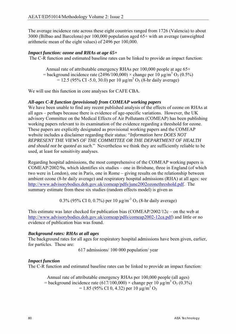
AEAT/ED51014/Methodology Volume 2: Issue 2
80 AEA Technology
The average incidence rate across these eight countries ranged from 1726 (Valencia) to about 3000 (Bilbao and Barcelona) per 100,000 population aged 65+ with an average (unweighted arithmetic mean of the eight values) of 2496 per 100,000. Impact function: ozone and RHAs at age 65+ The C-R function and estimated baseline rates can be linked to provide an impact function:
Annual rate of attributable emergency RHAs per 100,000 people at age 65+ = background incidence rate (2496/100,000) × change per 10 µg/m3 O3 (0.5%)
= 12.5 (95% CI -5.0, 30.0) per 10 µg/m3 O3 (8-hr daily average) We will use this function in core analyses for CAFE CBA. All-ages C-R function (provisional) from COMEAP working papers We have been unable to find any recent published analysis of the effects of ozone on RHAs at all ages � perhaps because there is evidence of age-specific variations. However, the UK advisory Committee on the Medical Effects of Air Pollutants (COMEAP) has been publishing working papers relevant to its examination of the evidence regarding a threshold for ozone. These papers are explicitly designated as provisional working papers and the COMEAP website includes a disclaimer regarding their status: �Information here DOES NOT REPRESENT THE VIEWS OF THE COMMITTEE OR THE DEPARTMENT OF HEALTH and should not be quoted as such.� Nevertheless we think they are sufficiently reliable to be used, at least for sensitivity analyses. Regarding hospital admissions, the most comprehensive of the COMEAP working papers is COMEAP/2002/9a, which identifies six studies � one in Brisbane, three in England (of which two were in London), one in Paris, one in Rome � giving results on the relationship between ambient ozone (8-hr daily average) and respiratory hospital admissions (RHA) at all ages: see http://www.advisorybodies.doh.gov.uk/comeap/pdfs/june2002ozonethreshold.pdf. The summary estimate from these six studies (random effects model) is given as
0.3% (95% CI 0, 0.7%) per 10 µg/m-3 O3 (8-hr daily average) This estimate was later checked for publication bias (COMEAP/2002/12c � on the web at http://www.advisorybodies.doh.gov.uk/comeap/pdfs/comeap2002-12ca.pdf) and little or no evidence of publication bias was found. Background rates: RHAs at all ages The background rates for all ages for respiratory hospital admissions have been given, earlier, for particles. These are:
617 admissions/ 100 000 population/ year Impact function The C-R function and estimated baseline rates can be linked to provide an impact function:
Annual rate of attributable emergency RHAs per 100,000 people (all ages) = background incidence rate (617/100,000) × change per 10 µg/m3 O3 (0.3%)
= 1.85 (95% CI 0, 4.32) per 10 µg/m3 O3

AEAT/ED51014/Methodology Volume 2: Issue 2
AEA Technology 81
This can be used in sensitivity analyses, as a check on consistency or in situations where baseline RHAs at age 65+ are unavailable.
10.1.4 Consultations with primary care physicians (general practitioners)
There is evidence from studies in London that daily variations in ambient particles, and/or ozone, and other gaseous pollutants, are associated with consultations with primary care physicians (i.e. general practitioners, in the UK context) (Hajat et al. 1999, 2001 and 2002). The 1999 study was based on numbers of people consulting (including home visits) in a 3-year period 1992-94, among a large population of about 282 000 (range varied from 268 718 � 295 740) registered patients from 45-47 practices in the Greater London Area. Because of differences in health care systems, it is difficult to know to what extent these relationships are transferable in Europe. We therefore use them in sensitivity analyses only, to help assess if these endpoints are important ones for quantifying the effects of ambient PM. PM and consultations for asthma C-R function In adults (though not in children) there was a consistent association between ambient PM10 and consultations for asthma (Hajat et al., 1999). Results are given (Hajat et al., Table 5), for all-year and separately by season (warm, i.e. April � September; cool, i.e. October - March); and separately for children (0-14), adults (15-64) and elderly (65+). Following suitable adjustment for confounding factors, associations with PM among adults and the elderly were statistically significant, and among children were almost statistically significant, for the warm season but not for the cool. Corresponding analyses showed no evidence that higher ozone led to increased consultations for asthma, nor did they show consistent relationships between PM and lower respiratory diseases. Coefficients for LRD were generally positive but not statistically significant; and, following the authors, we focus here on the relationships between PM and asthma, that were shown more consistently. Converting from a warm season pollution increment of 30.1 µg/m3 PM10, as given in Table 5, to the standard pollution change of 10 µg/m3 PM10, gives the following age-specific C-R functions (warm season only):
0-14: 2.5% (95% CI 0.0%, 5.2%) 15-64: 3.1% (95% CI 1.2%, 5.0%) and 65+: 6.3% (95% CI 2.1%, 11.2%)
Background consultation rates The mean daily numbers of consultations for asthma, by age group, in the warm season, are given (Hajat et al., Table 1) as 12.1 (age 0-14); 17.6 (age 15-64) and 3.3 (age 65+). The age-distribution of the patients is not given. However Hajat et al. (2001), studying the same population over the same time periods, report that there were 44 406 � 49 596 (say 47 000) children aged 0-14; and 185 267 � 204 039 (say, 195 000) adults aged 15-64 among the patients registered. We obtain, by difference from the total of 282 000, an estimated 40 000 elderly people (65+).
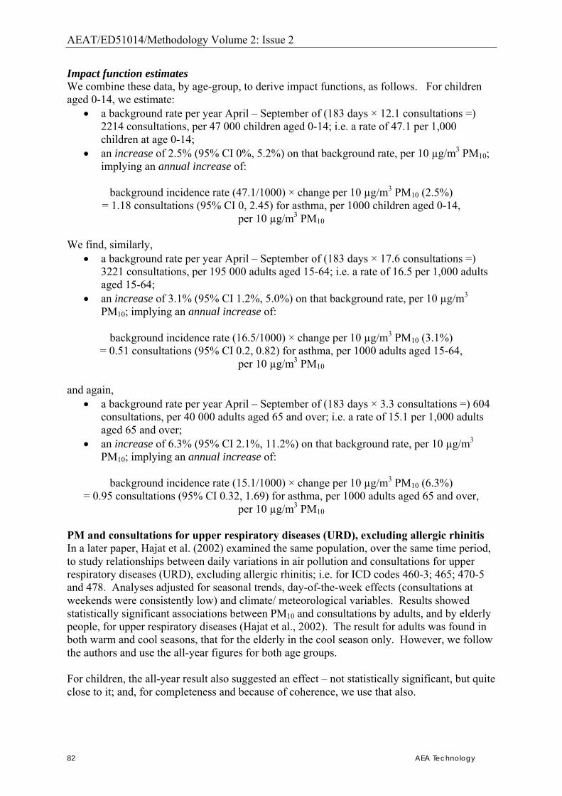
AEAT/ED51014/Methodology Volume 2: Issue 2
82 AEA Technology
Impact function estimates We combine these data, by age-group, to derive impact functions, as follows. For children aged 0-14, we estimate:
• a background rate per year April � September of (183 days × 12.1 consultations =) 2214 consultations, per 47 000 children aged 0-14; i.e. a rate of 47.1 per 1,000 children at age 0-14;
• an increase of 2.5% (95% CI 0%, 5.2%) on that background rate, per 10 µg/m3 PM10; implying an annual increase of:
background incidence rate (47.1/1000) × change per 10 µg/m3 PM10 (2.5%)
= 1.18 consultations (95% CI 0, 2.45) for asthma, per 1000 children aged 0-14, per 10 µg/m3 PM10
We find, similarly,
• a background rate per year April � September of (183 days × 17.6 consultations =) 3221 consultations, per 195 000 adults aged 15-64; i.e. a rate of 16.5 per 1,000 adults aged 15-64;
• an increase of 3.1% (95% CI 1.2%, 5.0%) on that background rate, per 10 µg/m3 PM10; implying an annual increase of:
background incidence rate (16.5/1000) × change per 10 µg/m3 PM10 (3.1%)
= 0.51 consultations (95% CI 0.2, 0.82) for asthma, per 1000 adults aged 15-64, per 10 µg/m3 PM10
and again,
• a background rate per year April � September of (183 days × 3.3 consultations =) 604 consultations, per 40 000 adults aged 65 and over; i.e. a rate of 15.1 per 1,000 adults aged 65 and over;
• an increase of 6.3% (95% CI 2.1%, 11.2%) on that background rate, per 10 µg/m3 PM10; implying an annual increase of:
background incidence rate (15.1/1000) × change per 10 µg/m3 PM10 (6.3%)
= 0.95 consultations (95% CI 0.32, 1.69) for asthma, per 1000 adults aged 65 and over, per 10 µg/m3 PM10
PM and consultations for upper respiratory diseases (URD), excluding allergic rhinitis In a later paper, Hajat et al. (2002) examined the same population, over the same time period, to study relationships between daily variations in air pollution and consultations for upper respiratory diseases (URD), excluding allergic rhinitis; i.e. for ICD codes 460-3; 465; 470-5 and 478. Analyses adjusted for seasonal trends, day-of-the-week effects (consultations at weekends were consistently low) and climate/ meteorological variables. Results showed statistically significant associations between PM10 and consultations by adults, and by elderly people, for upper respiratory diseases (Hajat et al., 2002). The result for adults was found in both warm and cool seasons, that for the elderly in the cool season only. However, we follow the authors and use the all-year figures for both age groups. For children, the all-year result also suggested an effect � not statistically significant, but quite close to it; and, for completeness and because of coherence, we use that also.
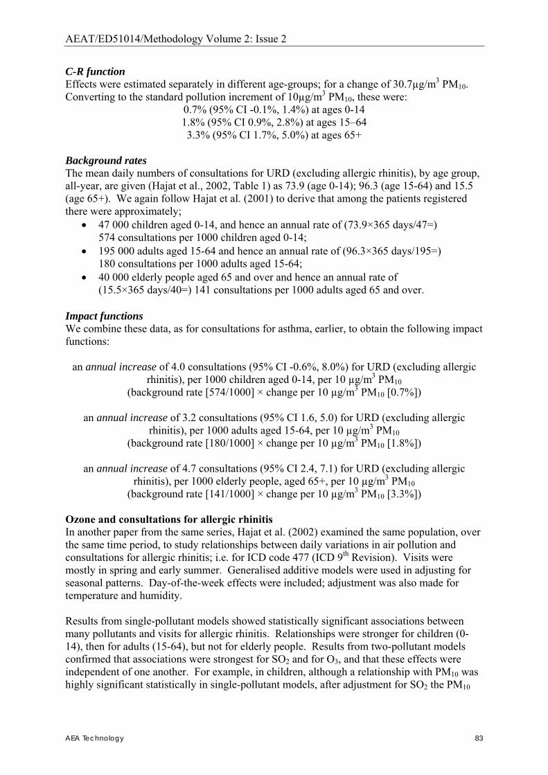
AEAT/ED51014/Methodology Volume 2: Issue 2
AEA Technology 83
C-R function Effects were estimated separately in different age-groups; for a change of 30.7µg/m3 PM10. Converting to the standard pollution increment of 10µg/m3 PM10, these were:
0.7% (95% CI -0.1%, 1.4%) at ages 0-14 1.8% (95% CI 0.9%, 2.8%) at ages 15�64 3.3% (95% CI 1.7%, 5.0%) at ages 65+
Background rates The mean daily numbers of consultations for URD (excluding allergic rhinitis), by age group, all-year, are given (Hajat et al., 2002, Table 1) as 73.9 (age 0-14); 96.3 (age 15-64) and 15.5 (age 65+). We again follow Hajat et al. (2001) to derive that among the patients registered there were approximately;
• 47 000 children aged 0-14, and hence an annual rate of (73.9×365 days/47=) 574 consultations per 1000 children aged 0-14;
• 195 000 adults aged 15-64 and hence an annual rate of (96.3×365 days/195=) 180 consultations per 1000 adults aged 15-64;
• 40 000 elderly people aged 65 and over and hence an annual rate of (15.5×365 days/40=) 141 consultations per 1000 adults aged 65 and over.
Impact functions We combine these data, as for consultations for asthma, earlier, to obtain the following impact functions:
an annual increase of 4.0 consultations (95% CI -0.6%, 8.0%) for URD (excluding allergic rhinitis), per 1000 children aged 0-14, per 10 µg/m3 PM10
(background rate [574/1000] × change per 10 µg/m3 PM10 [0.7%])
an annual increase of 3.2 consultations (95% CI 1.6, 5.0) for URD (excluding allergic rhinitis), per 1000 adults aged 15-64, per 10 µg/m3 PM10
(background rate [180/1000] × change per 10 µg/m3 PM10 [1.8%])
an annual increase of 4.7 consultations (95% CI 2.4, 7.1) for URD (excluding allergic rhinitis), per 1000 elderly people, aged 65+, per 10 µg/m3 PM10
(background rate [141/1000] × change per 10 µg/m3 PM10 [3.3%]) Ozone and consultations for allergic rhinitis In another paper from the same series, Hajat et al. (2002) examined the same population, over the same time period, to study relationships between daily variations in air pollution and consultations for allergic rhinitis; i.e. for ICD code 477 (ICD 9th Revision). Visits were mostly in spring and early summer. Generalised additive models were used in adjusting for seasonal patterns. Day-of-the-week effects were included; adjustment was also made for temperature and humidity. Results from single-pollutant models showed statistically significant associations between many pollutants and visits for allergic rhinitis. Relationships were stronger for children (0-14), then for adults (15-64), but not for elderly people. Results from two-pollutant models confirmed that associations were strongest for SO2 and for O3, and that these effects were independent of one another. For example, in children, although a relationship with PM10 was highly significant statistically in single-pollutant models, after adjustment for SO2 the PM10
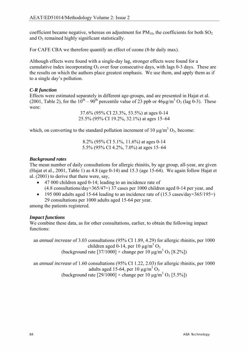
AEAT/ED51014/Methodology Volume 2: Issue 2
84 AEA Technology
coefficient became negative, whereas on adjustment for PM10, the coefficients for both SO2 and O3 remained highly significant statistically. For CAFE CBA we therefore quantify an effect of ozone (8-hr daily max). Although effects were found with a single-day lag, stronger effects were found for a cumulative index incorporating O3 over four consecutive days, with lags 0-3 days. These are the results on which the authors place greatest emphasis. We use them, and apply them as if to a single day�s pollution. C-R function Effects were estimated separately in different age-groups, and are presented in Hajat et al. (2001, Table 2), for the 10th � 90th percentile value of 23 ppb or 46µg/m3 O3 (lag 0-3). These were:
37.6% (95% CI 23.3%, 53.5%) at ages 0-14 25.5% (95% CI 19.2%, 32.1%) at ages 15�64
which, on converting to the standard pollution increment of 10 µg/m3 O3, become:
8.2% (95% CI 5.1%, 11.6%) at ages 0-14 5.5% (95% CI 4.2%, 7.0%) at ages 15�64
Background rates The mean number of daily consultations for allergic rhinitis, by age group, all-year, are given (Hajat et al., 2001, Table 1) as 4.8 (age 0-14) and 15.3 (age 15-64). We again follow Hajat et al. (2001) to derive that there were, say,
• 47 000 children aged 0-14; leading to an incidence rate of (4.8 consultations/day×365/47=) 37 cases per 1000 children aged 0-14 per year, and
• 195 000 adults aged 15-64 leading to an incidence rate of (15.3 cases/day×365/195=) 29 consultations per 1000 adults aged 15-64 per year.
among the patients registered. Impact functions We combine these data, as for other consultations, earlier, to obtain the following impact functions:
an annual increase of 3.03 consultations (95% CI 1.89, 4.29) for allergic rhinitis, per 1000 children aged 0-14, per 10 µg/m3 O3
(background rate [37/1000] × change per 10 µg/m3 O3 [8.2%])
an annual increase of 1.60 consultations (95% CI 1.22, 2.03) for allergic rhinitis, per 1000 adults aged 15-64, per 10 µg/m3 O3
(background rate [29/1000] × change per 10 µg/m3 O3 [5.5%])
AEAT/ED51014/Methodology Volume 2: Issue 2
AEA Technology 85
10.2. Air pollution and restrictions on usual activities
10.2.1 Definitions; choice of study – the US Health Interview Study (HIS)
Most major HIAs of air pollution and health include estimates of the effect of air pollution on days when normal activities are restricted � see, for example, ExternE (1995, 1999); Künzli et al. (2000); the US EPA Benefits Analysis for the Clean Air Act. Various endpoints have been studied, typically using C-R functions derived from Ostro (1987) or Ostro and Rothschild (1989). Both of these studies used data from six consecutive years (1976-81) of the Health Interview Study (HIS), carried out annually by the National Center for Health Statistics (NCHS) in the USA. Both focus on adults aged 18-64. Ostro (1987) analyses results for all adults in that age range, though with some analyses specific to people in employment. Ostro and Rothschild (1989) studied only people in employment because their days are more structured, implying more consistent activities, more consistent pattern of exposure to outdoor air pollutants, and more reliable recall of events. A restricted activity day (RAD) is a day when a study subject is forced to alter his or her normal activity, for health-related reasons. Within the HIS, RADs are classified in three mutually exclusive categories, according to degrees of severity (Portney and Mullahy, 1986):
• bed disability days • work or school loss days � only work loss days (WLDs) are relevant to the age-groups
studied; and • minor restricted activity days (MRADs) � these do not involve work loss or bed
disability, but do include some noticeable limitation on �normal� activity. In addition, days of restricted activity can be attributed to respiratory conditions, or not. Summary of methods of design, statistical analysis, and derivation of C-R function The HIS is a multi-stage probability sample of 50,000 households from metropolitan areas of all sizes and regions throughout the USA (Ostro and Rothschild, 1989). The data are based on interviews, implying that results for some individuals are provided by a proxy respondent, usually a close family member. They focus on events in the two weeks prior to interview. Both papers use Poisson regression analyses of the number of events (e.g. RADs, WLDs and MRADs) per subject in a two-week period. Adjustments were made for between-city differences (e.g. in factors such as time spent out of doors, building construction, and health practices) by using a fixed effects model, which focused the analysis on how individual observations differed from their city means. Air pollution was included as the relevant two week average of particulate matter, estimated from airport visibility data as fine particles (PM2.5). Adjustment was also made for other possible confounding factors such as sex, race, education, income, and average (daily) minimum temperature in the two week period of recall for each individual. Summary results, including coefficients of the effect of air pollution, and their associated SEs, are reported for each individual year 1976-81. In line with the original papers, and other HIAs � e.g. Abt Associates (2003) we use a unified coefficient, derived as the weighted mean of the six individual coefficients, with weights inversely proportional to the variances of the coefficients. More recently, Stieb et al. (2002) reported findings on air pollution and disability days from Canada�s National Population Health Survey (NPHS). This is a study similar in design to the
AEAT/ED51014/Methodology Volume 2: Issue 2
86 AEA Technology
US HIS, but carried out every two years. Because RADs are influential in the final HIA results, and because studies of RADs and air pollution are rare, we summarise their findings also.
10.2.2 Restricted activity days (RADs) and PM2.5 (Ostro, 1987) A 'restricted activity day' is defined as a day where a person needs to change his/her normal activities because of (ill-) health. It is based on questions asked at surveys of the general population (there are surveys in the USA, and corresponding surveys in Canada and the UK) In terms of decreasing severity, RADS include: • Days when a person needs to stay in bed; • Days when a person stays off work or school (or whatever may be their usual place to go,
if they have a usual place to go) but doesn't need to stay in bed; • Other, less serious, restrictions on normal activity. (These are what are called 'minor'
RADs, or MRADs.). C-R function Ostro (1987) studied both RADs and WLDs among adults aged 18-64 (total population, not just people currently employed) in separate analyses for each of the six years 1976-81. The great majority (85-95%) of subjects reported no restricted activity days. Results for RADs, based on about 12,000 subjects per year from 68 metropolitan areas, showed a consistent relationship with PM2.5: the coefficient for each of the six years 1976-81 was positive and highly significant statistically (p<0.01) (Ostro, 1987, Table 3). The estimated size ranged from 0.00284 to 0.00900, leading to a unified estimate of 0.00475 (SE 0.00029), and so we estimate an effect of PM as:
0.475% (95% CI 0.417%,0.533%) per µg/m3 PM2.5 Background rates The US Coal Fuel Cycle Report (ORNL/RFF, 1994) gives a background rate of 19 RADs per person per year, equivalent to a prevalence of 5.2%. Stieb et al. (2002) found the same baseline rate in Canada � see below. Note however that the General Household Survey in the UK (2002) reported higher numbers on average � about 25 RADs annually at age 16-44 and 43 annually at age 45-64. We do not know if the UK numbers are typical for elsewhere in Europe; we therefore use the background rate of 19 RADs per person per year as the baseline rate in the present analysis. Impact function Linking this background rate with the percentage increase of 0.475% per µg/m3 PM2.5 gives the following annual increase:
Increase in RADs per 1,000 adults per year at age 15-64: 902 (95% CI 792, 1013) per 10 µg/m3 PM2.5
Calculated as: baseline rate (19/person/year)× change per µg/m3 PM2.5 (0.475%)× 10 µg/m3 PM2.5×1000 adults
AEAT/ED51014/Methodology Volume 2: Issue 2
AEA Technology 87
Note that ExternE (1999) used lower values, to account for what was then understood as more severe effects of acute exposure to PM in US studies compared with Europe. This no longer applies. In the main analyses of RADS, we apply the impact function to people at ages 15-64. In sensitivity analyses, we use the same impact function but applied to all ages Stieb et al. (2002) Stieb et al. studied data from three cycles (1994-95, 1996-97 and 1998-99) of the Canadian NPHS, focussing on Toronto. �Disability days� were defined as days spent in bed or days when the respondent cut down on usual activities, during the two weeks prior to interview � a definition similar to that of Ostro (1987). Based on 5309 interviews, the mean number of disability days in the previous two weeks was 0.73, implying on average 19 disability days per person per year � the same background incidence rate as Ostro (1987) for RADs. Pollutants examined included PM10, PM2.5, coarse particles, NO2, SO2 and CO. These were characterised as two-week averages of daily pollution concentrations. Several statistically significant relationships were found. In single-pollutant models for the entire year, and adjusting for other factors, the strongest relationship statistically was with PM2.5, then with CO. However, there was evidence of non-linearity in the entire-year relationship with PM2.5 (a steep slope from low values of about 4 µg/m3 PM2.5 up to about 17 µg/m3 PM2.5 � the 95th percentile was 21.5 µg/m3 PM2.5 ). Also, in multi-pollutant models, CO persisted through the stepwise process whereas PM2.5 did not. Stieb et al. suggest that this may be due, at least in part, to the fact that PM measurements were available for every sixth day, only. Adapting from Stieb et al. Table 3, we find that the percentage increase in disability days per 10 µg/m3 PM2.5 was estimated as 33% (95% CI 6% - 58%) � figures that appear very large. Stieb et al. suggest that this may be due in part to using not daily but average two-week pollution concentrations. Another contributory factor is that the size of the effect was estimated over what appears to be much the steepest part of the (non-linear) C-R curve. This study gives some reassurance that; • there is a relationship between disability days and ambient air pollution, including and
perhaps especially ambient PM; • the background incidence rates of RADs in Ostro (1987) are reasonable; and that • the estimated coefficient from Ostro et al. is not necessarily high. We continue however to base quantification on Ostro (1987). For the analysis of RADs in CAFE, we need to make assumptions on the fraction of each type of RAD or minorRADs (see definitions above) that the functions quantify to ensure the appropriate valuation. Whilst several studies, including Stieb et al (2002), provide some evidence on the split in severity of restricted activity days, there is no definitive information. This is not surprising, given that the end point is culturally specific. As a result there are certain to be major differences from place to place, and so the uncertainty in transfer of rates from place to place will be large. The position defined for the CAFE-CBA has been developed taking account of our objective of developing a set of results that neither
AEAT/ED51014/Methodology Volume 2: Issue 2
88 AEA Technology
systematically over-estimate or under-estimate the health effects of air pollution. Evidence from the Stieb study shows that around on quarter to one third of RADs were bed disability days. We take the following as a plausible scenario. For working age adults: 25% of RADs are days when a person needs to stay in bed, 25% when they are off work but not in bed, and 50% mRADs. For people aged >65, we assume 33% are days when a person needs to stay in bed and 67% mRADs.
10.2.3 Work loss days (WLDs) Concentration-response function Again, we use Ostro (1987), where analyses each year were based on a unique sample of about 7000 employed adults aged 15-64 years. The estimated year-by-year coefficients were more variable than for RADs. Nevertheless, four of the six coefficients were positive and statistically significant (one was negative and statistically significant), and for three of the years the estimate was practically the same. Combining across years, as before, gave an overall estimate of 0.00460 (SE 0.00036)
0.46% increase in WLDs (95% CI 0.39%, 0.53%) per µg/m3 PM2.5 Because of year-by-year variability we also calculated a trimmed estimate, discarding the highest and lowest of the six coefficients, and based a weighted mean coefficient on the remaining four. This gave a very similar estimate of 0.495%. Background data in Europe This is derived in two parts:
i. average WLDs per individual in employment, aged up to 64; and ii. the total employment rate, defined as employed persons as a share of total population
of same gender and age Regarding WLDs per individual in employment, Bergendorff (2003) provides a summary in English of a study by Bergendorff at al. (2002). This compared sickness absence rates in eight European countries (Finland, France, Denmark, Germany, the Netherlands, Norway, Sweden and UK), using data from the relevant Labour Force Surveys (LFS) in each country. These LFS data are obtained by interview, where participants are asked about absences from work for the entire reference week considered by the survey. Thus, this study takes no account of absences shorter than one week; or, indeed, of some absences of a week or more, where these are spread across consecutive weeks. Results showed that crude (i.e. not age-standardised) absence rates varied across the eight countries, from 1.4% in Germany to 4.2% in Sweden. The eight-country average was 2.1%. Assuming 228 working days per year, this implies an average of 4.8 WLD per person per year, attributable to absences of at least one week�s duration. Bliksvaer and Helliesen (1997) reported figures that were broadly similar, including for some additional countries in Europe. There are other absences, of shorter duration. A study on sickness absence in the UK Civil Service reports (their Chart 7) that 30% of total days lost were accounted for by absences of less than one week�s duration. In a separate study, of employee absence 2003 in the UK, it is reported that the percentage of total days lost per year attributable to absences of less than one
AEAT/ED51014/Methodology Volume 2: Issue 2
AEA Technology 89
week is lower in public service workers than in workers in private services or in manufacturing and production. We may conclude that the estimated average of 4.8 WLD per person attributable to absences of one week or longer should be scaled upwards, by a factor of at least 1.5, to give an estimate of total annual days lost, per person. Thus, we use a background rate of 7.2 WLD per person per year, as a crude overall Europe-wide estimate of the background rates of WLD, among people in employment. The total employment rate in the EU25 in 2003 was 63.0% (males 70.9%, females 55.1%) among people aged 15-64 (Data from Eurostat). Country-specific data are available. Combining the 63% employment rate with the average number of work loss days (7.2) we derive a crude estimate of
4.5 WLDs per year per person aged 15-64 (general population) Impact function Linking together the information presented above we derive the following impact function: 207 WLDs (95%CI 176-238) per 10 µg/m3 PM2.5 per 1000 people aged 15-64 in the general population, calculated as: baseline rate (4.5 WLDs/person/year)× change per µg/m3 PM2.5
(0.46%)×10 µg/m3 PM2.5×1000 adults
10.2.4 Minor restricted activity days (MRADs): Ostro and Rothschild, 1989
Minor RADs are 'minor' restrictions on normal activity because of ill-health. Ostro and Rothschild (1989) considered the same six years of the HIS (1976-1981), and focused on minor (MRADs) and respiratory (RRADs) restricted activity days. Only current workers, resident in urban areas, were included; i.e. the population studied was less representative of the total population. Again, Poisson regression was used, in separate year-by-year analyses of the data. Two-week averages of the daily ozone levels (daily 1-hr max. in µg/m3) were used in the analysis; the PM2.5 data were the same as for Ostro (1987). Results are reported for single- and for two-pollutant models. We use the two-pollutant results, i.e. where as well as adjusting for city differences and various individual-level socio-economic confounders, the regression coefficients for ozone were also adjusted for PM2.5, and conversely. Background rates Ostro and Rothschild (1989) report a mean MRAD of 7.8 days per year, among people in employment aged 18-64. This is likely to be an under-estimate of overall rates in the 18-64 age group, because people in employment are on average healthier, and better off socio-economically, than those who are unemployed.
AEAT/ED51014/Methodology Volume 2: Issue 2
90 AEA Technology
However, in the absence of other data, we use the baseline rate of 7.8 MRADs per person and apply it to all adults aged 18-64, in the core analyses. In sensitivity analyses, we extend this to all adults � an extrapolation beyond the study, but an extrapolation which addresses what is almost certainly a real effect, and indeed is likely to under-estimate it. MRADs and PM2.5 C-R function There was a clear and consistent relationship between PM2.5 and respiratory RADs, with a coefficient which was positive, consistent and statistically significant in all six years. However, we quantify the milder endpoint of MRADs, as a surrogate for general symptoms among adults in the general population. The coefficients for MRADs and PM2.5 were more variable � four of six were positive and statistically significant; one was negative and statistically significant, and the 6th was positive and not significant. The derived weighted average was 0.00741 (SE 0.00070):
0.74% (95% CI 0.60%, 0.88%) per µg/m3 PM2.5 After trimming the two extreme coefficients, the weighted mean of the remaining four was almost identical, at 0.77% Impact function Linking the C-R function and the baseline estimate we obtain an increase of
577 MRADs (95% CI 468-686) per 10 µg/m3 PM2.5 per 1000 adults aged 18-64 per year, calculated as baseline rate (7.8 MRADs/person/year) × change per µg/m3 PM2.5 (0.74%) ×
10 µg/m3 PM2.5 × 1000 adults
AEAT/ED51014/Methodology Volume 2: Issue 2
AEA Technology 91
MRADs and ozone C-R function Perhaps surprisingly, there was no clear or consistent relationship linking ozone and respiratory RADs. There was however a reasonably strong and consistent relationship between MRADs and ozone. The regression coefficients for the six years were again very variable with most (including two negative) being statistically significant individually. The weighted mean was derived as 0.00111 (SE 0.00034) giving an increase of;
0.111% (95% CI 0.043, 0.179) per µg/m3 O3 (1-hr max) or
1.48% (95% CI 0.57%, 2.38%) per 10 µg/m3 O3 (daily 8-hr average) using a conversion factor of 1.33 based on Schwarz (1997). Impact function Linking with baseline rates we derive the following impact function:
Increase in MRADs = 115 (95% CI 44, 186) per 10 µg/m3 ozone (8-hr daily average) per 1000 adults aged 18-64 per year, calculated as baseline rate (7.8 MRADs/person/year)×
change per 10 µg/m3 O3 (1.48%)×1000 adults
Note: These MRAD functions will be applied to all adults, including those over 65, in sensitivity analysis.
10.3. Effects of PM and ozone on medication use by people with asthma
10.3.1 Brief remarks on medication use by people with asthma The WHO meta-analysis of acute effects studies in Europe also examined medication use � bronchodilator usage or specific use of β agonists � among people with chronic respiratory symptoms. The evaluation took account of children and adults. Information is from panel studies. Medication use applies to people with asthma, although the panel studies considered were not restricted to people with asthma. We have noted that hospital admissions may be planned or emergency admissions, and that air pollution affects emergency rather than planned admissions. Similarly, people using medication to control asthma may follow a planned maintenance programme, or use supplementary medication to control symptoms, or both. Maintenance medication includes the planned use of inhaled corticosteroids; supplementary medication includes the on-demand use of bronchodilators, for example short-acting β2 agonist. It is to be expected that daily variations in air pollution will affect the supplementary use of medication to control asthmatic symptoms and asthma attacks. For that reason, studies of air pollution and medication use in people with asthma focus on the use of bronchodilators. However, von Klot et al. (2002) found relationships with maintenance medication also, where use of the maintenance medication had been intermittent, e.g. discontinued during periods of good health.
AEAT/ED51014/Methodology Volume 2: Issue 2
92 AEA Technology
In understanding the effects of air pollution on people with asthma, the importance of bronchodilator usage has been described well by Just et al. (2002): �In well-treated asthmatics, weaker associations between pollutant levels and asthma attacks or asthma-like symptoms would be expected, because asthmatics with an efficient maintenance treatment are able to manage their symptoms with supplementary medication.� Consequently, the effects of air pollution on people with asthma may be more discernible via associations with supplementary medication use rather than via associations with asthma attacks and/or symptoms.
10.3.2 Medication use by children with asthma Bronchodilator usage and ambient particles (PM10) C-R function The WHO meta-analysis gives estimates, for changes in days of bronchodilator usage, in relation both to PM10 and to black smoke (BS). Both sets of estimates come from studies in 31 locations, including 27 locations from the PEACE study. PEACE was a very large multi-centre study of children aged 6-12, with chronic respiratory symptoms indicating asthma, enrolled and studied during the winter of 1993-94 in one rural and one urban location near each of 14 centres in Europe. (Data from one urban location were missing). The results of the PEACE study were generally negative regarding the effects of daily air pollution on lung function, daily symptoms and medication usage in these children. This was unexpected and contrary to the findings of several other panels. Roemer et al. (2000) speculate that the relatively short study period of two months or less may have made the study vulnerable to complex time-related patterns and specific events � for example, the influenza epidemic which occurred in Europe in the winter of 1993-94. Considering the evidence as a whole, the soon-to-be-published WHO review of The Health Effects of Air Pollution on Children�s Health and Development concludes that there is sufficient evidence to assume a causal relationship between air pollution exposure and aggravation of asthma in children; and, as noted earlier, one way that such a relationship may show is via increased medication usage. Results from the WHO meta-analysis of PM and bronchodilator usage showed that neither pooled estimate (for PM10 or for BS) was statistically significant. For PM10 the meta-analysis gives a pooled estimate of the odds ratio of
1.005 (95% CI 0.981, 1.029) per 10 µg/m3 PM10 which is quite far from statistical significance at the usual 5% limit. (The odds ratio of 1.005 is approximately the same as a percentage increase of 0.5%, if the background rates are small.) Background rates There are three components to the background rates:
i. The age-groups to which the result will be applied; ii. The percentage of children in that age-group who meet the criteria for inclusion in a
panel such as was studied; and iii. The percentage of such children who, on average, use respiratory medication on any
given day.
AEAT/ED51014/Methodology Volume 2: Issue 2
AEA Technology 93
Regarding age ranges, the PEACE study is based on children aged 6-12 yr; the background data are in 5-yr age-groups; and so we will apply the results at ages 5-14 yr. Regarding the percentage of children in that age-group that meets the criteria for chronic symptoms for inclusion in a panel such as was studied, we note that the criteria for inclusion in the PEACE study were that children reported that they had
a. in the previous 12 months: wheeze (apart from colds) AND/OR attacks of shortness of breath (with wheezing) AND/OR dry cough (apart from colds)
b. AND/OR doctor diagnosed asthma ever in life. In Europe, the ISAAC Study (International Study if Asthma and Allergies in Childhood) gives prevalences of asthma-related respiratory symptoms in two age-groups (6-7 yr and 13-14yr) in centres in many countries of Europe (ISAAC Steering Committee, 1998) and worldwide.
i. Regional 12-month prevalences in Northern and Eastern Europe (including centres in Estonia, Latvia, Poland and Sweden) were:
• for children aged 13-14: wheeze, 9.2%; night cough 12.2%; ever had asthma, 4.4%; and
• at ages 6-7: wheeze, 8.8%; night cough 11.4%; ever had asthma 3.2%.
ii. Corresponding regional 12-month prevalences in Western Europe (including centres in Austria, Belgium, France, Germany, Greece, Italy, Portugal, Spain and the UK) were:
• for children aged 13-14: wheeze, 16.7%; night cough 27.1%; ever had asthma, 13.0%; and
• at ages 6-7: wheeze, 8.1%; night cough 16.1%; ever had asthma 7.2%.
On that basis we estimate that approximately 15% of children in Northern and Eastern Europe, and 25% of children in Western Europe, would qualify for panels such as were set up in the PEACE study. Finally, regarding the percentage of such children who, on average, use respiratory medication on any given day, then mean daily prevalences are reported in some of the panel studies. We have not tried to be comprehensive in obtaining such rates. For example, we seek all-year estimates and the PEACE study was winter-time only. In any case, the detailed papers from the PEACE study report background rates as incidences, whereas we need data as prevalences (i.e. average number of people with asthma using bronchodilators on any given day). However, a few studies indicate what mean daily prevalences might apply. (Only some of the studies investigating relationships between air pollution and medication usage report daily mean prevalence rates of bronchodilator usage.) Winter
• Roemer et al. (1993), studying 73 children aged 6-12 yr in two small towns in the east Netherlands Jan-March 1991, reported a daily mean prevalence of bronchodilator use of 10.2%. Inclusion criteria were broadly similar to those used later by PEACE.
• During three months in the winter of 1994, in eastern Finland, Timonen and Pekkanen (1997) studied panels of school children aged 7-12 yr who met the inclusion criteria
AEAT/ED51014/Methodology Volume 2: Issue 2
94 AEA Technology
for the PEACE study. Children were in two panels, one urban, one suburban, and were further subdivided into those with dry cough only, and those with other qualifying symptoms. The mean % using bronchodilators on any given day of the study period among asthmatic children was reported as 13% (urban, 39 children) and 30% (suburban, 35 children). None of the 95 children with cough as the only qualifying symptom used a bronchodilator. This gives a mean daily usage of 9.2% among all children studied. Note that 95 (56%) of the 169 children studied were included because of dry cough alone, and did not use bronchodilators.
• Segala et al. followed up 84 children aged 7-15 yr in Paris over six months November 1992 to may 1993. All had medically diagnosed asthma: 43 classed as mild, 41 severe, of whom respectively 37% and 27% used supplementary β2-agonists. The mean daily prevalence rate of usage was low: 2.9% in children with mild asthma, 0.8% in children with moderate asthma, 1.9% overall.
Spring/ summer
• Gielen et al. (1997) studied 79 children aged 7-13 yr from Amsterdam (the Netherlands) and nearby, mostly during a period concentrated on May and June 1995. These were selected from two special schools for children with chronic illnesses, mostly respiratory. For example, 77% had doctor-diagnosed asthma, implying on average greater severity of disease, and associated greater use of bronchodilators, than for the panels in the PEACE study. Results, based on 61 subjects with completed data for at least 60% of days, showed a mean daily prevalence of bronchodilator usage of 39% (min 26%, max 50%).
• Tiitanen et al. studied 49 children aged 8-13 years over 6 weeks in Eastern Finland. All met the inclusion criteria for PEACE; 26% had doctor-diagnosed asthma, 26% were taking medication for asthma. Daily prevalences were not reported directly; results (Tiitanen et al., Table 3) suggest however that the mean daily prevalence of bronchodilator usage was low, at about 4%.
Clearly, there is wide variation between studies. This seems to have several components:
• Differences between studies in study inclusion criteria � though we have aimed to standardise on criteria similar to the PEACE study;
• Differences in the proportions on asthma medication overall, and supplementary medication in particular. For example Peters et al. (1996), studying children aged 7-15 in former East Germany and the Czech Republic with a medical diagnosis of asthma, found that >80% of the children in East Germany used β2-agonists compared with about 20% of those in the Czech Republic;
• Among those with bronchodilators as supplementary medication, differences in mean daily usage.
Against that background, it seems that an estimate of 10% mean daily prevalence of bronchodilator usage among panels of school-children who meet the PEACE study criteria, is a reasonable first estimate for quantification.
AEAT/ED51014/Methodology Volume 2: Issue 2
AEA Technology 95
Impact function Linking, as usual, the C-R function with background rate, we estimate an impact function as follows:
Annual increase in days of bronchodilator usage = 180 (95% CI -690, 1060) per 10 µg/m3 PM10 calculated as baseline rate (10% daily
prevalence of bronchodilator use) × days per year (365) × change per 10 µg/m3 PM2.5 (0.5%) × 1000 children aged 5-14 years meeting the PEACE study criteria
with approximately 15% of children in Northern and Eastern Europe, 25% in Western Europe, meeting the inclusion criteria. Bronchodilator use (β2-agonist) and ozone C-R function The meta-analysis results refer to one study only, of the use of β2-agonist in a panel of 82 children aged 7-15 (mean 11) with medically diagnosed asthma, and who were taking daily anti-asthma treatment, followed up over a 3-month period in early summer (01 April to 30 June) in 1996 (Just et al., 2002). Those studied took a variety of medications, both planned and supplementary, to control their asthma. The relationship between ozone and asthma attacks and/or symptoms were complex, and were evident only when controlling also for interactions between O3 and temperature and between O3 and pollen count, for asthma attacks. A relationship between O3 and increased (supplementary) use of bronchodilators was found when analyses were restricted to days on which no corticosteroids were used by the children. The estimated odds ratio for supplementary bronchodilator use on those days was both high and statistically significant, at
1.41 (95% CI 1.05, 1.89) per 10 µg/m3 O3. Background rates Age-group to which results will be applied: The study included children aged 7-15. Given that the available population data are in 5-year age groups, we will apply the impact function to children aged 5-14. Among children aged 5-14, percentage of days ‘at risk’ of an ozone effect on bronchodilator usage: The study by Just et al. (2002) included only those with medically diagnosed asthma and who were taking daily anti-asthma treatment; it was a summer-time study; and effects were found only on days where corticosteroids were not being used. To obtain credible background rates, consider the following:
• The percentages of qualifying children will be less than the percentages quoted earlier, from the ISAAC study, of those who �ever had asthma� which, for Northern and Eastern Europe, were approximately 4%, for Western Europe approximately 10%.
• On the other hand, it is unclear what proportions of these are currently using medication to control asthma. However, percentages are likely to be greater than the percentages reporting severe asthmatic symptoms in the previous 12 months. For example, the ISAAC Steering Committee (1998) reported 12-month prevalences of �asthma attacks� as 2% in Northern and Eastern Europe, about 3% in Western Europe.

AEAT/ED51014/Methodology Volume 2: Issue 2
96 AEA Technology
• Taking these considerations into account, we will assume that about 60% of children aged 5-14, ever diagnosed as having asthma, are at risk.
• A further component is the percentage of days when people with asthma medication do not use corticosteroids to control their asthma. In Just et al. (2002) there were 979 person-days when subjects did not use corticosteroids, i.e. about one day in six of 5970 valid study observation person-days (82 subjects, 91 days studied, 80% data compliance days).
• The issue of �summer only� effects is dealt with in CAFE CBA by quantifying effects (core analyses) only when 8-hr daily ozone exceeds a cut-off point of 35ppb O3. We therefore develop a function as if the effect were all-year, leaving until later in the analysis the restriction of effects to days of higher ozone only.
• All things considered we will therefore use background rates of �days-at-risk-in-the-general-population� of 10% of person-days of people who ever had doctor-diagnosed asthma; i.e.
o 0.4% of person-days of all children aged 5-14 in Northern and Eastern Europe, or 1460 person-days annually, per 1000 children (general population)
o 1% of person-days of all children aged 5-14 in Western Europe, or 3650 person-days annually, per 1000 children (general population)
It is likely that the endpoint has, at most, a small influence on final numbers. It is also likely that results vary by country, implying that refinement of these background rates is difficult, and unlikely to matter much. Mean daily prevalence rates of bronchodilator usage by the ‘at risk’ population on ‘at risk’ days: This has been considered in examining PM and bronchodilator usage. Of the studies considered there, the one that most closely resembles the panel studied by Just et al. (2002) is that by Gielen et al. (1997), which reported a daily mean prevalence of 40%. We use that number in quantifying the ozone effects. Impact function We derive an impact function by linking the C-R function with background rates. Recall that the odds ratio, per 10 µg/m3 PM10, is 1.41 (95% CI 1.05, 1.89) per 10 µg/m3 O3, and the background rate (mean daily prevalence) among people in qualifying panels, on at-risk days, is 40%. Because the background rate is quite large, then we need to apply the ozone-related changes to the odds rather than to the probability of using a bronchodilator. Thus the background rate of 0.4 implies an odds of 0.4/(1-0.4), i.e. 0.4/0.6, or 0.666. With an odds ratio of 1.41 per 10 µg/m3 O3, this gives a new odds of 0.94, and equivalently a probability of 0.94/1.94, or 0.485, following an increase of 10 µg/m3 O3. Similar calculations apply to the 95% CI. We express these results as saying that an increase of 10 µg/m3 implies new background rates of 48.5% (95% CI 41.2%, 55.8%). Subtracting the original background incidence rate of 40% from these new figures gives (at typical background rates) an increase of:
0.085 (95% CI 0.012, 0.1558) per 10 µg/m3 O3 in the probability of bronchodilator use in an at-risk day. Applying this increase to the at-risk days (estimated as 1460 days annually, per 1000 children in the general population, Northern and Eastern Europe; 3650 days annually, Western Europe) we get
AEAT/ED51014/Methodology Volume 2: Issue 2
AEA Technology 97
annual increase in days of bronchodilator usage per 10 µg/m3 O3 per 1000 children age 5-14 years (general population)
= 124 (95% CI 18, 227) in Northern and Eastern Europe; = 310 (95% CI 44, 569) in Western Europe;
Comments This odds ratio is high. It is based on one study only, and it may well not be representative. Also, it has been necessary to make some assumptions in order to get estimates of some of the components of background data. On the other hand, medication use is an important health-related endpoint, and so it is appropriate that the derived impact function be included in at least some sensitivity analyses. This will provide a check on whether using an apparently high estimate suggests that quantification of this pathway might make an important contribution to the overall benefits of reducing air pollution.
10.3.3 Medication use by adults with asthma Bronchodilator usage and ambient particles (PM10) C-R function The WHO meta-analysis identified results from four locations, all in the Netherlands, all involving bronchodilator usage, and only one of which (Dusseldorp et al., 1995) was statistically significant. One of the studies was unusable in the meta-analysis; the other two locations came from a single study (van der Zee et al., 2000) whose risk estimates were much lower than those of Dusseldorp et al. (1995). Van der Zee et al. studied adults aged 50-70 years, with weak criteria for inclusion in their study. Dusseldorp et al. studied people aged 26-79 years, i.e. over a more representative age range, and included adults with more severe asthma. The study was however quite small (32 subjects), and possibly untypical in that it was intentionally focussed on people living near a steel factory. The WHO meta-analysis found a pooled odds ratio of
1.010 (95% CI 0.990, 1.031) per 10 µg/m3 PM10 i.e. positive, but not nearly statistically significant. Because it is well understood that air pollution leads to exacerbations of asthma, for completeness, we will use this estimate for quantification, despite its lack of statistical significance. Background rates Quantification requires suitable background rates. There are two components:
• mean daily prevalence of bronchodilator use by people with asthma; and • percentage of adults with asthma.
Regarding the mean daily prevalence of the use of bronchodilators by people with asthma, as a 1st approximation we derive estimates from some panel studies of air pollution and health. (Indeed, an internet (Google) search on �daily prevalence� AND (bronchodilator OR agonist) revealed little other than studies of air pollution and medication use.)
AEAT/ED51014/Methodology Volume 2: Issue 2
98 AEA Technology
• Dusseldorp et al. (1995, Table 5) reported a 43.3% background rate (mean daily prevalence) of bronchodilator usage in their study October-December 1993 of 32 adults in the Netherlands who had been prescribed medication in the previous few years because of obstructive airways disease.
• Von Klot et al. (2002) studied 53 patients with asthma � either (i) doctor-diagnosed, or (ii) self-reported with �asthma�, together with reported asthmatic symptoms in the previous 12 months � over the winter of 1996-97. All 53 used medication to control asthma; for 42 (79%), this included short-acting β2 agonist. Daily mean prevalence of the use of β2-agonists in this subset was also 79%, implying a daily mean prevalence of 62% in the panel as a whole.
• Hiltermann et al. (1998) studied 60 non-smoking patients aged 18-55 with intermittent to severe persistent asthma, over three summer-time months (July-Sept 1995), near Leiden in the Netherlands. 85% of the panel used bronchodilators. The daily mean prevalence in the panel as a whole was 32% (Hiltermann et al., Table 3), implying a daily mean prevalence of 38% among bronchodilator users.
We examined whether suitable data could be obtained from the European Community Respiratory Health Survey (ERCHS), a very large multi-centre study of adults aged 20-44 at time of 1st survey (ERCHS1). The main paper reporting country-specific prevalences (ERCHS, 1996) has limited information on the % of people using asthma medication, but no information on daily frequency of use. Janson et al. (1997: Eur Respir J 10: 1795-1802), studying a sample of ECRHS1, report substantially more data on medication usage, though again with limited information about daily usage. The authors reported strong country-related differences in usage. Any estimate will be at best approximate, if applied to other countries and locations. With the reasonably stringent definition of asthma proposed, it seems reasonable to use an all-year supplementary medication (i.e. bronchodilator) usage rate of 50%, among adults with established asthma, as a means of giving 1st estimates. Results will then show if the endpoint merits further work to refine the background rates. For implementation we need an estimate of the percentage of adults with asthma, of a severity comparable to that of the panels studied; i.e. sufficiently severe that on-demand medication is frequently used by them. We use data from the European Community Respiratory Health Survey (ERCHS), a very large multi-centre study of adults aged 20-44 at time of 1st survey (ERCHS1). A detailed paper (ERCHS, 1996, Eur Respir J 9: 687-695, Table 3) reports prevalences of various conditions from that survey. The table gives results from 40 centres in Europe and 8 elsewhere (4 in New Zealand). The median prevalences of people who use asthma medication, and of people diagnosed as having asthma (i.e. reporting an asthma attack and/or using asthma medication) were, respectively, 3.1% and 4.5%, across the study as a whole. The paper doesn�t distinguish between different kinds of asthma medication.
• Age-related variations in asthma prevalence are not particularly strong, and so these data may be used for adults generally.
• There are major variations in prevalences between countries in Europe. In broad terms, prevalences are lower in Eastern Europe and higher in Western Europe. For
AEAT/ED51014/Methodology Volume 2: Issue 2
AEA Technology 99
example, reported prevalences of people having asthma in Estonia (1 centre) were 2.2%; Greece (1 centre) 2.9%; Austria (1 centre) 3.1%; Norway (1 centre) 4.3%: Sweden ( 3 centres) 5.8-6.8%; The Netherlands (3 centres) 4.3-4.7%; France (5 centres) 3.5-5.5%; UK (4 centres) 7.5-8.4%.
• Nevertheless, as a 1st approximation, while establishing the importance of this endpoint for CAFE CBA, it seems reasonable to use the median value of 4.5% with ‘asthma’ , as a global estimate, for Europe, of the percentage of adults with asthma of a severity that corresponds to the panels studied. Country-specific estimates can be used if the endpoint proves to be important, or if more accurate local estimates are required.
• The median value of 4.5% is inflated marginally, as an estimate in Europe in 1996, by inclusion of New Zealand and some other high-prevalence locations outside of Europe. This however is likely to be offset by the continuing increase in people with asthma.
Note that the other Dutch study, by van der Zee et al. (2000), had a much less stringent definition of asthma for inclusion in its panels (implying a higher proportion of the general population qualified), and a correspondingly lower daily prevalence rate of asthma medication usage. Together, these imply a percentage of days of bronchodilator usage in the general population not very different from what we have estimated. Impact function, for adults with well-established asthma As usual, we link the C-R function with background rates, to derive an impact function. The C-R function was given as an odds ratio of 1.010 (95% CI 0.990, 1.031) per 10 µg/m3 PM10. Applied to a background probability of 0.5 of daily usage, this gives an increase in probability of daily usage of
0.0025 (95% CI -0.0025, 0.0076) per 10 µg/m3 PM10 implying an impact function of an increase in bronchodilator usage days of
912 (95% CI -912, 2774) per year per 10 µg/m3 PM10 per 1000 adults aged 20+ with well-established asthma (say, 4.5% of the adult population)
Medication (bronchodilator) use by adults with asthma, and ozone Background The WHO meta-analysis identified two relevant studies. One of these, by Hiltermann et al. (1998), has been described briefly, above. Ozone was represented as daily max 8-hr moving average; its relationship to daily prevalence of bronchodilator usage was positive (OR 1.009 per 10 µg/m3 O3) but not statistically significant (95% CI 0.997, 1.020) at the selected lag of 1 day. However, when 7-day cumulative ozone was considered, the estimated effect was higher and statistically significant; in the authors� view, bronchodilator use was associated with ozone. The second study (Higgins et al., 1995) was based on 75 subjects with asthma or COPD in North-West England, but followed up for at most four weeks each during August-September. All gaseous pollutants were represented as 24-hr daily averages; measurements of PM were not available. Results, from multi-pollutant models, showed a highly statistically significant relationship between (24-hr average) O3 and daily bronchodilator usage: OR 1.44 (95% CI 1.14, 1.82) per 10 µg/m3 O3. It appears that temperature was not adjusted for in these
AEAT/ED51014/Methodology Volume 2: Issue 2
100 AEA Technology
analyses; the text on relationships with lung function (PEF) reports that relationships were not significantly affected by the inclusion of daily temperature in the model. C-R function Together these studies suggest that there is an effect to be quantified, though based on limited information. For consistency with the WHO meta-analysis, and so with the general recommendations of this CAFE CBA, we quantify using results from analyses based on daily 8-hr ozone, and adjusting for climate and other confounders. Thus, we use results from Hiltermann et al. (1998). We also continue to use the WHO meta-analysis selected lag of 1 day, although it falls short of statistical significance, giving a C-R function of:
Odds ratio 1.009 (95% CI 0.997, 1.020) per 10 µg/m3 O3 It may be that this C-R function under-estimates the effects of ozone on bronchodilator usage in asthmatic adults. Background rates We use summer-time rather than all-year background rates, because these are likely to be more relevant to ozone concentrations above 35ppb 8-hr daily mean. These summertime rates are estimated from Hiltermann et al. (1998), giving a mean daily prevalence of 32%, as noted earlier. Impact function Linking change in odds ratio to the probability (0.32) of daily usage in a �typical� panel of people with persistent asthma (estimated as 4.5% of the general adult population � see earlier) we find an increase in probability of daily usage of
0.0020 (95% CI -0.0007, 0.0043) per 10 µg/m3 O3 or
730 days (95% CI -255, 1570) per 10 µg/m3 O3 per 1000 adults aged 20+ with persistent asthma (say, 4.5% of the adult population)
10.4. PM, ozone, and respiratory symptoms
10.4.1 Introductory remarks about studies of respiratory symptoms As for medication usage, information on the relationship between respiratory symptoms and air pollution is derived from panel studies of individuals, followed up daily over periods of weeks or months.
10.4.2 PM and acute respiratory symptoms in children The WHO meta-analysis considered panels of children with asthma of various severities or chronic respiratory symptoms. As for medication usage, information on PM and effects in children with chronic respiratory conditions was dominated by the PEACE study (see, e.g. Roemer et al., 1999). Because this was a study of winter-time pollution, it does not give information about the effects of ozone on the health of children with chronic respiratory conditions.
AEAT/ED51014/Methodology Volume 2: Issue 2
AEA Technology 101
PM10, cough and other respiratory symptoms in children with chronic respiratory conditions Cough Cough in children with chronic respiratory disease was one of the endpoints considered in the WHO meta-analysis of air pollution studies in Europe. Results, dominated by the PEACE study, were generally negative; the WHO meta-analysis gives a summary odds ratio of almost exactly 1, i.e. no consistent or overall evidence of an adverse effect. As noted earlier, there were some specific limitations on the ability of the PEACE study to detect effects (short time series together with a concurrent influenza epidemic), and it is widely recognised that air pollution does exacerbate asthma. Nevertheless, in view of these findings, we do not attempt to quantify a relationship between cough and ambient PM specifically in children with asthma. We do, however, quantify an effect of lower respiratory symptoms (LRS), including cough, on children in the general population, which of course includes children with asthma � see later. Other symptoms in children with respiratory diseases Several studies of children with symptoms indicating chronic respiratory diseases (�symptomatic children�) show associations between daily occurrence of lower respiratory symptoms (LRS) and daily air pollution, notably but not only PM. Such studies were reviewed recently by Ward and Ayres (2004), as part of a wider review of panel studies of particulate air pollution and respiratory effects in children. Ward and Ayres reviewed 22 studies, the majority of which concerned panels of symptomatic children. These studies showed evidence of an effect of daily variations in PM10 and/or PM2.5 on lung function (PEF1 � peak expiratory flow in one second) and on LRS. There was some, though less convincing, evidence for an association between PM and cough also. This indicative evidence came largely because, in contrast to the WHO meta-analysis, the meta-analysis of Ward and Ayres was (i) not restricted to European studies, and effect estimates in published US studies seemed generally higher than in Europe; (ii) included the generally negative overall results from the PEACE study as overall results from a single study only, whereas the WHO meta-analysis included 27 separate panels from PEACE; and (iii) included general population panels as well as panels of symptomatic children. In this context, Ward and Ayres (2004) found that:
• There were effects also in general population panels of children, i.e. in panels that had not been selected on the basis of pre-existing respiratory symptoms/ conditions;
• In limited within-study comparisons, there was no convincing or consistent evidence that effects (estimated relative risks) were more severe in symptomatic children compared with general population panels
• Somewhat more extensive between-study comparisons suggested that risks were higher in general population panels. This may be related to location � a greater proportion of general population studies had been carried out in the USA, and risks seemed higher in US studies generally.
Nevertheless, the systematic review by Ward and Ayres (2004) very strongly suggests that effects of PM on respiratory symptoms should be quantified for children generally, and not be confined to children with chronic symptoms; and it is on that basis that we proceed.
AEAT/ED51014/Methodology Volume 2: Issue 2
102 AEA Technology
PM and lower respiratory symptoms (LRS), including cough, among children in the general population C-R function As noted above, Ward and Ayres (2004) reviewed panel studies of the effects of PM on lower respiratory symptoms and on cough in children generally. The exact definition of LRS can vary between studies, but usually includes wheezing, chest tightness, shortness of breath, and possibly cough. (Ward and Ayres excluded from their meta-analysis of LRS any studies that considered cough only, but included studies with wheeze only.) The meta-analysis results showed that the estimated relative risks from PM were very similar for LRS and for cough, though overall meta-analysis results, using a fixed-effects (FE) statistical model, were not statistically significant for cough. Fixed effects estimates are appropriate when the various studies give results that are sufficiently similar that they can be taken as estimating the same underlying risk. When this is so, it gives greater confidence in extrapolating the results beyond the locations studied. There was however considerable heterogeneity between studies, possibly reflecting differences in study methods as well as real but unexplained differences in risk estimates in different locations and seasons. When this heterogeneity was taken into account, using random effects (RE) methods of meta-analysis, the estimated RR was greater for both LRS and cough, and was also statistically significant for both outcomes. Results showed a pooled relative risk (random effects model) of
• 1.004 (95% CI 1.002, 1.006) for cough, per µg/m3 PM10, based on 12 studies (Ward and Ayres, Table 3) and
• 1.004 (95% CI 1.002, 1.005) for LRS, per µg/m3 PM10, based on 16 studies (Ward and Ayres, Table 4).
We use the C-R function for cough (i.e. that with the wider CI), with the intention of applying it to LRS also, giving an estimated odds ratio of:
• 1.04 (95% CI 1.02, 1.06) per 10 µg/m3 PM10 Relevant population The meta-analysis studies were typically of panels of 6-11 years of age, though some studies included in the meta-analysis of LRS included children up to age 13 or 15. The population data for CAFE CBA are in 5-year age-groups. We will quantify at ages 5-14 years. Background rates We need data on background rates (mean daily prevalence) of days with LRS, including cough. We do not know of any large-scale general population multi-centre study that provides such information directly. One approach to obtaining the information indirectly is to identify available (European) panel studies of children in the general population and from them obtain the relevant background rates (daily prevalences of LRS), if these are reported. An alternative strategy also involves using data on daily prevalences from available panel studies, and is a 2-stage process:
• Identify available (European) panel studies of children with chronic respiratory symptoms;
• Obtain from them the background rates (daily prevalences of LRS) in this symptomatic sub-group; and
AEAT/ED51014/Methodology Volume 2: Issue 2
AEA Technology 103
• Link this with information on the prevalence, in the general population, of children with chronic respiratory symptoms.
In effect, this second approach is a quantification among symptomatic children only, and so we focus on the general population approach (1st strategy). Obtaining rates from general population panel studies As an indication of background rates in the general population, we consider two general population studies from the Netherlands � one based in the winter months, one in spring/ early summer. Winter period: On each of three consecutive winters, 1992-3 to 1994-5, Van der Zee et al. (1999) studied children in two areas in the Netherlands, one urban area, one rural, usually different areas and always different children studied each winter. Basic descriptive results (van der Zee et al., Table 2) are presented aggregated over all three winters, but separately by urban/ rural location, and by whether or not the children had chronic respiratory symptoms, using the similar criteria to the PEACE study. Children were considered as �with symptoms� if they had:
• asthma attacks in the past 12 year � shortness of breath, with wheezing; • chronic cough in the past year � at least three months; • doctor diagnosed asthma (ever) • treated by a specialist for asthma, in past 12 months; • wheezy chest in past 12 months, apart from a cold
and as �no symptoms� otherwise. The study was designed to include about 200 children in each of the four panels defined by urban/ rural, and by with or without symptoms; in practice, there were 396 children with and 396 without symptoms, giving a large panel study. Of those with symptoms, 26% urban, 38% non-urban, had doctor diagnosed asthma; 16% urban, 24% rural, used medication daily. Note that the �general population� is a mixture of children with and without symptoms, and so we need to aggregate across panels, with suitable weighting. Lower respiratory symptoms (LRS) were defined as shortness of breath, wheeze, shortness of breath with wheeze; upper respiratory symptoms (URS) as sore throat, or runny or stuffed nose. Cough and phlegm were considered separately from LRS, URS and from one another. In both panels, with symptoms and without, there were only small differences between urban and non-urban children in their mean daily prevalences of symptoms.
• Among those with symptoms, the mean daily prevalence was: cough 35%, LRS 8.8%. • Among those without symptoms, corresponding results were: cough 17%, LRS 1.0%. • A general population estimate (weighted mean, assuming that 25% of children
qualified for the panel with symptoms � see earlier, ISAAC study, Western Europe) therefore gives an overall estimated mean daily prevalence of 21% cough, 3% LRS. Using weights for Northern and Eastern Europe (15% with chronic symptoms) gives overall estimates of 20% cough, 2% LRS � well within any estimation errors. All estimates apply to the winter season.
Summer period: Hoek and Brunekreef (1995) studied a general population sample of 300 children 7-11 years from 5 primary schools in two rural towns in the Netherlands, over 102 days from late March to end June 1989. Note that 45/300 (15%) had one or more chronic respiratory symptoms.
AEAT/ED51014/Methodology Volume 2: Issue 2
104 AEA Technology
LRS was defined as wheeze, chest tightness, shortness of breath, or phlegm production; URS as sneezing, or runny or stuffed nose. Throat symptoms were defined as hoarseness or throat pain. The mean daily prevalence of cough was 5.4%, of LRS 1.5%. All-year estimates We estimate all-year background mean daily prevalence rates as the unweighted average of winter and summer estimates, giving:
• Cough: 13% • LRS, excluding cough: 2%; and so • LRS, including cough: 15%
Impact function Recall that the estimated odds ratio for cough and for LRS was 1.04 (95% CI 1.02, 1.06) per 10 µg/m3 PM10. Linking this with the background rate of 15% gives an estimated new rate of 15.51% (95% CI 15.25%, 15.76%) i.e. an increase of 0.0051 (95% CI 0.0025, 0.0076) in the probability of daily average occurrence of LRS (including cough), giving
an estimated increase of 1.86 (95% CI 0.92, 2.77) extra symptoms days per year per child aged 5-14, per 10 µg/m3 PM10, calculated simply by multiplying the
increase in probability of daily average occurrence by 365 days. Comment: This estimate is about five times as large as the corresponding estimate of 577 MRADs (95% CI 468-686) per 10 µg/m3 PM2.5 among adults aged 15-64 (using a conversion factor of PM2.5 = 0.65PM10). This gives some greater confidence in both sets of results, which were derived in very different ways, from studies of quite different designs, and apply to different age groups. Note that had we used the fixed effects estimate of 1.001 per µg/m3 PM10 for LRS from Ward and Ayres (2004), rather than the random effects estimate of 1.004, then the two sets of results would have been very similar.
10.4.3 Ozone and acute respiratory symptoms in children Most available studies are based on panels followed up during the spring or summer months when, because (i) ozone levels are higher, (ii) daily variations in ozone are greater and (iii) children spend more time outdoors, there is a greater possibility than in winter of detecting an adverse effect of ozone. 8-hr daily ozone and respiratory symptoms in children with chronic respiratory conditions The WHO meta-analysis gave an estimate from one study only � in Paris, by Just et al. (2002). Summary details of this study have been given earlier, where we have used it in quantifying an effect of O3 on bronchodilator usage in children. Data are given for nocturnal cough. Cough: Just et al. (2002) studied nocturnal cough, giving results both for incidence and for prevalence. (In this study, mean daily prevalence of cough was 7.9, mean daily incidence 3.1, implying an average duration of 2.5 days per episode.) The WHO meta-analysis, in
AEAT/ED51014/Methodology Volume 2: Issue 2
AEA Technology 105
accordance with the conventions it adopted, reported results for incident episodes, giving, at the selected lag of 0 days, a high odds ratio of 1.04 per 10 µg/m3 O3 but with a very wide 95% CI also (0.920, 1.176). The corresponding OR for prevalent episodes, again at lag 0, was the same, at 1.04 per 10 µg/m3 O3, but with a shorter 95% CI of (0.97, 1.10). Wheeze was reported as not being associated with any of the pollutants examined. O3 and respiratory symptoms among children in the general population General remarks The WHO meta-analysis focuses on cough in children with chronic respiratory symptoms. We do not know of any recent published meta-analysis of the effects of ozone on respiratory symptoms, based on studies world-wide or on European studies in particular, that focuses on respiratory symptoms other than cough, and on the general population as well as on children with corresponds to the WHO meta-analysis, or to the meta-analysis of Ward and Ayres (2004) for PM and respiratory effects in children. However, the effects of ozone on health are currently being reviewed by the Committee on the Medical Effects of Air Pollutants in the UK, as part of a wider assessment of the evidence regarding a threshold (or not) for the effects of ozone on health. The current working conclusions of that review (Heather Walton, 2004, personal communication) include that: • There is convincing evidence that daily variations in ozone are associated with lower
respiratory symptoms, including cough; whereas the evidence for an association with upper respiratory symptoms is more equivocal;
• Effects on LRS/ cough/ phlegm are not restricted to people with chronic respiratory symptoms, e.g. asthma; indeed, there is no strong evidence that relative risks (in practice, odds ratios) are higher among people with chronic respiratory disease than among the general population.
On that basis, we aim to quantify an effect of LRS, including cough and/or phlegm, among people in the general population, where practicable using studies carried out in Europe, examining symptoms prevalences in relation to 8-r daily max O3. As part of the COMEAP review the St. George�s Hospital database, which was also used for the WHO meta-analyses, was examined for studies linking daily ozone with respiratory symptoms. The search revealed (Richard Atkinson, 2004, personal communication) one study in Europe examining symptoms prevalence in relation to 8-hr daily ozone among children in the general population, that in Armentieres, Northern France, by Declerq and Macquet (2000). We use results from that study for quantification of respiratory effects in the general population in Europe. Declerq and Macquet (2000) studied 91 children (including seven who were asthmatic) from the general population in Armentieres, Northern France, in the early summer (April to June), in relation to ozone and other pollutants. In separate analyses, daily prevalence of cough and phlegm, and of breathing problems (difficulty breathing, wheeze, asthma attack), were associated with 8-hr daily max O3. The relevant C-R functions were as follows: C-R function for prevalence of cough:
Odds ratio 1.05 (95% CI 0.99, 1.12) per 10 µg/m3 O3.
AEAT/ED51014/Methodology Volume 2: Issue 2
106 AEA Technology
C-R function for prevalence of “breathing problems”, i.e. for lower respiratory symptoms (LRS), excluding cough and phlegm
Odds ratio 1.03 (95% CI 0.92, 1.15) per 10 µg/m3 O3 which, given the definition of �breathing problems�, we apply to LRS (excluding cough). Background rates for LRS, including cough Earlier � see the Section on PM and respiratory symptoms in children � we considered sources of data on mean daily prevalences of LRS (including cough) in children in Europe. We examined results from some relevant panel studies, distinguishing by season because background rates in winter are higher. In CAFE CBA the effects of ozone are estimated for the core analysis only when daily max O3 exceeds a cut-off point of 35ppb (or 70 µg/m3 O3). Because ozone concentrations are higher in summer than in winter, we consider it more appropriate to use background rates relevant to summer only. • As noted earlier, Hoek and Brunekreef (1995) reported mean daily prevalences of 5.4%
for cough, and of 1.5% for LRS defined as wheeze, chest tightness, shortness of breath, or phlegm production, in a general population sample of 300 children 7-11 years in the Netherlands, studied between late March and end June.
Impact function for LRS, excluding cough, among children in the general population As usual, we derive impact functions by linking C-R functions and background prevalence rates. We do this separately for cough and for LRS (excluding cough). Applying the odds ratios of the C-R function to the background odds of 0.01523 gives an estimated impact of:
an increase of 0.16 (95% CI -0.43, 0.81) days of LRS (excluding cough) per child aged 5-14 years, per 10 µg/m3 O3, per year
Impact function for cough among children in the general population Similarly, applying the odds ratios for cough to the background odds of 0.0571 gives an estimated impact of:
an increase of 0.93 (95% CI -0.19, 2.22) cough days per child aged 5-14 years, per 10 µg/m3 O3, per year
10.4.4 PM and respiratory symptoms in adults General remarks; strategy The WHO meta-analysis of studies in Europe considered cough in adults with respiratory disease. The panels studied included adults with asthma, chronic respiratory symptoms, chronic obstructive pulmonary (airway) disease and bronchial hyper-responsiveness. Again, we do not know of any recent meta-analysis or review of (i) other symptoms among people with chronic respiratory conditions or (ii) the effects of PM on respiratory symptoms among adults generally. With regard to other symptoms among people with chronic respiratory conditions, we have examined the five source papers that the WHO meta-analysis identified as panel studies in
AEAT/ED51014/Methodology Volume 2: Issue 2
AEA Technology 107
Europe informative about PM10 and cough, and derived information about other symptoms also. In doing so we have focused on lower respiratory symptoms, given that other pathways have identified LRS as particularly relevant to PM and children, and to ozone (children and adults). We have not attempted to review systematically the evidence regarding PM and respiratory symptoms in general population panels of adults. However, the following is relevant:
• This is an endpoint which has been quantified by ExternE (in 1995, though not in 1999), and by other HIAs also, using a large general population panel study of adults, about 70% of whom were aged 30-44 years, in southern California. From that study, Krupnick et al. (1990) give results for prevalence of symptoms generally while Ostro et al. (1993) studied in more detail the incidence of LRS in non-smoking adults from the same study.
• One of the European studies of PM and respiratory symptoms in adults with chronic respiratory conditions also included an urban and a non-urban panel of non-symptomatic adults in the general population (van der Zee et al., 2000). This was a study of adults aged 50-70 years over each of three winters (1992-93 to 1994-95) in the Netherlands. In each year, four panels were studied: one each of adults with and without chronic respiratory symptoms, in an urban and non-urban location. (Different panels of subjects were studied each winter, usually in different locations.) The screening questions each year were based on the ECRHS questionnaire; subjects were included in the symptomatic panels if they reported a positive answer to one or more of six questions about wheeze or asthma, or to one or more of five questions about chronic cough and/or phlegm. Thus, the criteria for the symptomatic panels were weak/ inclusive, and consequently the non-symptomatic panels were highly selected for good respiratory health.
• In the non-symptomatic panels (274 adults, most of whom were followed up for about three months), van der Zee et al. (2000) found no consistent associations between daily respiratory symptoms in winter and the air pollutants studied, including PM10, in either the urban or the non-urban areas. There was evidence of an effect on URS at lag one day, with the same estimated odds ratio of 1.020 per 10 µg/m3 PM10 in both the urban and the non-urban panels, though not statistically significant in either, and with no evidence of an effect at lag 0 or 2 days. Detailed results for LRS were not given.
• In discussing these results, van der Zee et al. (2000) reported that, to their knowledge, the southern California study was the only other panel study at that time of air pollution and respiratory symptoms among adults not selected for chronic respiratory symptoms. (Note that the non-symptomatic panels of van der Zee et al. were selected for good respiratory health, and so are not representative of the general population, which is in fact a mixture of non-symptomatic and symptomatic adults.)
• On the basis of these generally negative results about PM and respiratory symptoms from a winter-time study of a relatively large panel of non-symptomatic adults in the Netherlands, we have some doubts about transferring to Europe the positive results of a single, though also large-scale, study of PM and respiratory symptoms in California. Insofar as there is an effect in the general population, it seems that it can be approximated by estimating the effects in symptomatic adults only, especially if the resulting C-R functions are applied to a large subset of the population, i.e. using an inclusive rather than a strict definition of who is symptomatic.
• On that basis, for CAFE CBA we quantify effects in symptomatic adults only.
AEAT/ED51014/Methodology Volume 2: Issue 2
108 AEA Technology
PM10, cough and other respiratory symptoms in adults with chronic respiratory symptoms (�symptomatic adults�) Cough and PM: C-R function The meta-analysis identified six panels in Europe which examined cough (or nocturnal cough or cough and phlegm) in adults, in relation to PM10. Results from three of these studies (two from the Netherlands: Dusseldorp et al., 1995, and Boezen et al., 1998; and one from Paris: Neukirch et al., 1998) were used in the meta-analysis, giving an estimated odds ratio of
1.043 (95% CI 1.005, 1.084) per 10 µg/m3 PM10,
i.e. just significant statistically at the 5% level. None of the other three studies was statistically significant.
• One, by van der Zee et al. (2001), studied urban and rural panels in the Netherlands, and reported that relationships between cough and PM10 were not statistically significant.
• Results from the final study, by Hiltermann et al. (1998), were excluded on the grounds that they were reported as relative risks rather than as odds ratios, and so were not comparable with the odds ratio estimates of the other panels. Its estimated relative risk was, however, less than 1, at 0.986 (95% CI 0.963, 1.008) per 10 µg/m3 PM10.
• It appears that the panels studied by Boezen et al. (1998), in the winter of 1993-94, were in fact a subset of the data studied by van der Zee et al. (2001), who used data from three winters in the Netherlands. A strong case can therefore be made for giving priority to the generally negative results from the larger, 3-winter, study rather than the positive results from one winter which were reported separately. (The separate reporting was because Boezen et al. analysed by sub-groups in ways that van der Zee et al. were unable to do.)
• Finally, where a study reported results both for prevalence and incidence, the WHO meta-analysis used the incidence results. Neukirch et al. (1998) reported both sets of results, in a study of out-patients with mild to moderate asthma, in Paris. The meta-analysis used the incidence odds ratio of 1.116 (95% CI 1.052, 1.183) per 10 µg/m3 PM10 � an unusually high relative risk. The corresponding prevalence odds ratio was lower, at 1.059 (95% CI 0.998, 1.123) per 10 µg/m3 PM10.
It follows that the meta-analysis would have been lower had it been possible to include results from all six panels, and had it been based on prevalence studies. We think that a relationship between PM10 and cough in symptomatic adults should be quantified, but that the meta-analysis estimate may be too high to be representative, and that it is best regarded as an upper estimate. Before finally deciding what estimate to use, we consider other respiratory symptoms in these same panels, focusing on lower respiratory symptoms. Lower respiratory symptoms (LRS) and PM10 in symptomatic adults As discussed above, we do not include the results of Boezen et al. (1998), regarding these as superseded by van der Zee et al. (2000). Neukirch et al. (1998) studied 40 non-smoking adult out-patients aged 16-70 years, with mild to moderate asthma (at least one asthma attack in the previous 12 months, but not on maintenance steroids) over 6 months November 1992 to May 1993, in Paris. Results are
AEAT/ED51014/Methodology Volume 2: Issue 2
AEA Technology 109
reported both for incidence and for prevalence. The background daily mean prevalence rate of wheeze was 15.1%, with 45.7% for shortness of breath and 20.1% for nocturnal cough. The odds ratio for wheeze in relation to PM was estimated as:
1.059 (95% CI 0.998, 1.123) per 10 µg/m3 PM10 The lag time, of 6 days, is suspiciously long. Shortness of breath was associated with PM10 in the small subset of 17 people who took supplementary medication (β2-agonists) on an as-needed basis. Hiltermann et al. (1998) studied 60 adults aged 18-55 yr with intermittent to severe asthma (85% used bronchodilators) in Leiden in the Netherlands. They reported a mean daily prevalence of 43% for shortness of breath during the study period of three summer months July-Sept 1995, and 34.5% for cough and/or phlegm on these days. The association between daily PM10 on daily presence or absence (i.e. prevalence) of shortness of breath was investigated using logistic regression. Results are reported as relative risks. It is unclear if these are odds ratios; we will use them as if they are. On that basis, the association between PM10 and days of shortness of breath was estimated as a relative risk of
1.032 (95% CI 1.006, 1.060) per 10 µg/m3 PM10 As described earlier, van der Zee et al. (2000) studied an urban and a non-urban panel of adults with at least one of 11 chronic respiratory symptoms, in each of three winters in the Netherlands. Background prevalence rates are not reported, nor are they in Boezen et al. (1998). Different adults were included each year; in total, analyses of the urban symptomatic panel were based on 138 subjects, the non-urban on 128. The estimated effects were:
Urban (lag 2 days): 1.002 (95% CI 0.985, 1.020) per 10 µg/m3 PM10 Non-Urban (lag 1 day): 1.005 (95% CI 0.995, 1.015) per 10 µg/m3 PM10
Dusseldorp et al. (1995) studied 32 adults with moderate to severe symptoms Oct-Dec 1993 near a steel mill in the Netherlands. Mean daily prevalence rates were cough 18.6%, shortness of breath 17.4% and wheezing, 8.1%. They reported very similar odds ratios of 1.46 and 1.49 respectively, per 100 µg/m3 PM10, for shortness of breath and for wheeze (2-day lag). We use the C-R function for shortness of breath, which was statistically significant, and apply it to LRS generally, to give and estimated effect of
1.038 (95% CI 1.010, 1.068) per 10 µg/m3 PM10 C-R function from meta-analysis of results from these 5 panels A random effects meta-analysis of results from all five panels gave an overall estimate of
1.017 (95% CI 1.002, 1.032) per 10 µg/m3 PM10 We will apply this estimate to LRS, including cough; and not include a specific estimate for cough.
AEAT/ED51014/Methodology Volume 2: Issue 2
110 AEA Technology
Background rates To implement, we need suitable background rates. • We can obtain estimates of background rates for relevant chronic respiratory disease from
the ECRHS study, though the papers we have available (e.g. ECRHS, 1996) are based on data for adults only up to age 44, and the prevalence of respiratory symptoms increases with age. ECRHS (1996) shows important country-related differences in prevalences; at this stage, we use the overall study median values. These are given as 20.7% for wheeze, 27.9% for cough at night � either of which would have qualified a subject for inclusion in the symptomatic panels of van der Zee et al. (2000). On that basis, an estimate of 30% is almost certainly an under-estimate of those with chronic respiratory symptoms. It may nevertheless be a reasonable estimate to use, because the evidence of PM effects came largely from studies of adults with more severe asthma.
• The mean daily prevalences of various respiratory symptoms from some of the panels have been given, above. In two of the three studies, it seems that the prevalence of LRS, including cough, is at least 50%; in the 3rd, the prevalence was lower. Noting that these were more severely ill panels than the symptomatic panels of van der Zee et al., we assume a mean daily prevalence rate of 30% for LRS, including cough, among symptomatic adults.
Impact function Applying the estimated odds ratios to the background probability of 0.30 (odds 0.43) that someone with chronic respiratory symptoms will report LRS (including cough or phlegm) on any given day, we get the following impact function:
Annual increase of 1.30 (95% CI 0.15, 2.43) symptom days i.e. lower respiratory symptoms, including cough,
per adult with chronic respiratory symptoms, per 10 µg/m3 PM10 where we estimate that 30% of the adult population qualify as having chronic respiratory symptoms.
10.4.5 Ozone and respiratory symptoms in adults Ozone, cough and other respiratory symptoms in adults with chronic respiratory symptoms (�symptomatic adults�) Cough The WHO meta-analysis identifies two relevant studies only � the same two panels as were studied for bronchodilator usage. Higgins et al. (1995) reports a positive association, with high odds ratio (1.050 per 10 µg/m3 O3) but not statistically significant (95% CI 0.910, 1.212), among adults with asthma in North-West England. On the other hand Hiltermann et al. (1998) found no evidence of an adverse effect in adults with asthma in Leiden in the Netherlands � they reported a negative coefficient of 0.987 per 10 µg/m3 O3 which just qualified as statistically significant at the usual 5% level (95% CI 0.987, 0.999). On that basis, we do not quantify an effect of ozone on daily cough specifically among adults with asthma. Instead, we quantify an effect of ozone on respiratory symptoms in the general population.
AEAT/ED51014/Methodology Volume 2: Issue 2
AEA Technology 111
Ozone and respiratory symptoms in adults in the general population This endpoint merits a full review, something that is outside the scope of what we can do for CAFE CBA. We have, in the past, used a study by Krupnick et al. (1990) as a basis for impact pathways for both PM and for O3 (ExternE, 1995), latterly for O3 only (ExternE, 1999). The same study was used in other major HIAs, both earlier (ORNL/RFF, 1994) and more recently. We have some reservations about using these C-R functions for CAFE CBA.
• These functions are based on a single study which may be unrepresentative, especially of conditions in Europe.
• The underlying study, though large, has a complex design and statistical analysis, requiring adjustment for many confounding factors (the analysis seems to have been done well).
• Calculations to derive impact factors are complex also � see e.g. ExternE (1995); and • Various approximate conversion factors are needed to express the pollutants in a
suitable form. Pending a proper review of PM, ozone and this important health endpoint, we will include in sensitivity analysis, to indicate possible upper bounds on an impact pathway that may be important. The following write-up is largely extracted and summarised from ExternE (1995, 1999) The study The impact functions for both PM and ozone are taken from the same study, Krupnick et al. (1990). This was a large panel study of 290 families (572 adults, 756 children) in California from September 1978 to March 1979.
• Most (about 70%) of the adults studied were aged 30-45. • The pollutants considered were daily exposure to ozone (daily 1-hr max.), the
coefficient of haze (COH) as a surrogate for fine particles (daily average), sulphur dioxide (daily average) and nitrogen dioxide (average of peak period).
• Health effects were measured as the presence or absence of any one of 19 respiratory-related symptoms or conditions, or headache, or eye irritation; about 1 in 24 (i.e. <5 %) of these symptoms were classed as �serious� (i.e. RAD or presence of fever or �sought medical advice.�)
A Markov process model was used to analyse the relationship between air pollution and these (mild) symptoms, thus taking into account that the probability of illness on any day is likely to be dependent on the occurrence or not of symptoms on the previous day. Logistic regression was used to model the probability of symptoms on any given day, with adjustment for the dependent variable lagged one day as one of several explanatory variables. The design was of daily pooled cross-sections over a longitudinal follow-up. Thus, possible confounding included both factors that varied day-by-day (temperature, rainfall humidity) but also a wide range of characteristics at the individual level. A major strength of the study was the use made of a very large number (74682) of person-days of observations on adults. This enabled careful modelling of different combinations of pollutants, while adjusting for numerous other covariates.

AEAT/ED51014/Methodology Volume 2: Issue 2
112 AEA Technology
Modelling suggested an important role both of particles (COH) and of ozone in relation to presence or absence of symptoms. The impact function for PM defined below is adjusted for the effects of ozone. Particles The relationships for COH were similar in adults and children, the results for adults were used to derive exposure-response relationships for all ages. The relationship between COH and the probability of reporting one of the symptoms is summarised by the logistic regression coefficient (log odds) of 0.0088 (SE = 0.0046) / 100 ft., adjusted for ozone. Using the conversion factor COH = 0.55 PM10 (Dockery and Pope, 1994), this result implies a mid-estimate of log-odds of change in symptom days as 0.0088 x 0.55 = 0.00484 (SE 0.00253), per µg/m3 PM10. The baseline probability of any (adult) subject reporting any symptom is given as 0.19. Following ExternE (1995), based on earlier work by Ostro, this resolves to:
Annual change in symptom days per 1000 people at risk (all ages) = 4650 (95% CI 210, 9090) per 10 µg/m3 PM10
Note: We think that this is a high estimate of the effects of PM on respiratory symptoms, especially for application in Europe. It is included here with the intention that it be used only for sensitivity analyses, to indicate how big an effect might be. The core analyses will use a function for symptoms in adults with chronic respiratory conditions, developed earlier from studies in Europe.
Ozone Results for ozone, adjusted for particles, are summarised by the regression coefficient 0.0055 (SE = 0.0027) per O3 (pphm), i.e. 0.00055 (SE = 0.00027) per O3 (ppb). These are results for adults; no significant relationship was found for children. The baseline probability of any (adult) subject reporting any symptom is given as 0.19. Following ExternE (1995, 1999), based on earlier work by Ostro, this resolves to:
Annual change in symptom days per 1000 people at risk (all ages) = 528 (95% CI 10, 1046) per 10 ppb O3 (1-hr max)
To convert to µg/m3, divide by 2; and multiply by 1.3 as an approximate conversion to 8-hr daily mean ozone to give:
Annual change in symptom days per 1000 people at risk (all ages) = 343 (95% CI 6, 692) per 10 µg/m3 O3 (8-hr daily max)
10.4.6 Final comments on respiratory symptoms and medication usage in adults and children
We have proposed quite a wide range of endpoints for quantification, as would be expected, given that air pollution (including both PM and ozone) is widely understood to exacerbate pre-existing chronic respiratory disease, including asthma. In doing so, however, we have used meta-analysis estimates based on very few studies (i.e. three studies or less); and

AEAT/ED51014/Methodology Volume 2: Issue 2
AEA Technology 113
estimated background rates for Europe as a whole based on panel studies of small numbers of individuals from a few countries in Western Europe, especially the Netherlands. These results from the WHO meta-analyses and the meta-analysis of Ward and Ayres (2004) supersede, for CAFE CBA, the quantifications in ExternE (1999) of particles in relation to bronchodilator usage, cough and lower respiratory symptoms in adults and children, and of asthma attacks in relation to ozone. Similarly, we will not use the specific functions for asthma attacks in children and adults as used by Künzli et al. (2000). Those earlier HIAs for exacerbation of asthma used impact functions which were less representative, and gave higher values than, those adopted now. Even so, they gave rise to impact estimates that, after monetary valuation, were small compared with those of other impact pathways such as chronic bronchitis or RADs (Hurley et al., 2000). A working conclusion might be that, for impact assessment, exacerbations of asthma identified as increases in cough and/or respiratory medication use are not very important compared with other impact pathways. However we consider that it is important to include them, for completeness; else, there is a deficient picture of the range of adverse effects attributable to air pollution and of the benefits to health of reducing it. If however it proves that these pathways have an important influence on the benefits analysis as a whole, then it will increase the importance of obtaining better background rates, and/or of refining as far as possible those presented here, to take account of known variations in the prevalences of respiratory disease across countries in Europe.
10.5. PM, ozone and minor changes in cardio respiratory function Finally, we note that it is well-established that ambient air pollution, especially ambient PM, adversely affects lung function and measures of cardiovascular functioning also. Lung function We have not focussed on lung function changes because, as noted elsewhere, these are not readily amenable to monetary valuation. Their omission may, however, give an incomplete picture of the adverse effects of air pollution. Heart rate variability and other associated indices Similarly, there have been studies showing relationships between ambient PM and a range of indices of cardiovascular functioning. Again, at present these endpoints are not amenable to monetary valuation, but the do form an important part of the overall effects, in that they add plausibility to the findings linking air pollution and more serious cardiovascular outcomes (mortality, hospital admissions) that have been quantified in the present study.
AEAT/ED51014/Methodology Volume 2: Issue 2
114 AEA Technology
10.6. Conclusion: Health impacts (morbidity) to be quantified Chronic exposure 1. New cases of chronic bronchitis � PM � core analysis Acute exposure 2. Respiratory hospital admissions:
• PM � core analysis • O3 � core analysis
3. Cardiac hospital admissions � PM � core analysis 4. Consultations with primary care physicians (general practitioners) in adults � PM �
• PM and consultations for asthma � sensitivity only • PM and consultations for upper respiratory symptoms (excluding allergic rhinitis)
� sensitivity only • Ozone and consultations for allergic rhinitis � sensitivity only
5. Restricted activity days (RADs) and PM � core analysis
• Note we assume that two-thirds of these are MRAD and value according. • We will also consider quantification of (i) Work Loss Days and PM as evidence of
more severe RADs and (ii) MRADs and PM as evidence of less severe RADs (possibly equivalent to symptom days)
6. Minor restricted activity days and ozone � core analysis 7. Use of respiratory medication by people with respiratory diseases � core analysis
• Children � PM � core analyses • Children � O3 � core analyses • Adults � PM � core analyses • Adults � O3 � core analyses
8. Symptom days
• PM � o LRS, including cough, among adults with chronic symptoms � core analyses o LRS, including cough, among children in the general population � core
analyses • O3 �
o Respiratory symptoms among adults in the general population � sensitivity analyses
o Cough and LRS (excluding cough) among children in the general population � core analyses
AEAT/ED51014/Methodology Volume 2: Issue 2
AEA Technology 115
11. Valuation of Morbidity
11.1. Introduction This section deals with morbidity effects alone. In reviewing the morbidity health end-points we use as our starting point the values derived in the recent ExternE work. There has been one major new empirical study on the valuation of these end-points, covering five countries across Europe - Ready et al. (2004) - and the pooled results of this study are used in the first instance when discussing the health end-points below. To clarify what we are valuing: the starting point for the valuation of health end-points is the identification of the components that comprise changes in welfare. These components should be summed to give the total welfare change, assuming no overlap between categories. The three components include: (i) Resource costs i.e. medical costs paid by the health service in a given country or
covered by insurance, and any other personal out-of-pocket expenses made by the individual (or family).
(ii) Opportunity costs i.e. the cost in terms of lost productivity (work time loss (or
performing at less than full capacity)) and the opportunity cost of leisure (leisure time loss) including non-paid work.
(iii) Dis-utility i.e. other social and economic costs including any restrictions on or reduced
enjoyment of desired leisure activities, discomfort or inconvenience (pain or suffering), anxiety about the future, and concern and inconvenience to family members and others.
The welfare changes represented by components (i) and (ii) can be proxied using market prices that exist for these items. This measure - in best practice - needs to be added to a measure of the affected individual's loss of utility, reflected in a valuation of the willingness-to-pay/accept (WTP/WTA), to avoid/compensate for the loss of welfare associated with the illness. Note that there is the possibility of overlap between components since, for example, the individual will include both financial and non-financial concerns in his/her assessment of loss of welfare. Financial costs are often not borne fully by the individual but are shared through health insurance and public health care provision. Thus, we assume here that the financial costs are separable and measured in component (i). If this is not the case, then a part of the dis-utility measured in the WTP estimate will be incorporated in the private medical costs associated with treatment (or prevention) of the health end-point, and the total valuation should be reduced by an equivalent amount.

AEAT/ED51014/Methodology Volume 2: Issue 2
116 AEA Technology
11.2. Cost estimates for specific endpoints
11.2.1 Component (i): Health care resource costs The generic unit costs for hospital-based health care are presented in the table below. The data has been derived from Netten and Curtis (2000), and MEDTAP International, reported in Ready et al. (2004). Since this data is based on public health care provision it is exempted from indirect taxes and is therefore expressed at factor cost. It has not been possible to derive unit cost data for all EU countries, but mean values calculated from the available data are presented and can be used as a first proxy for EU countries that currently do not report such values. Generic hospital costs are the average costs of a wide variety of specialist treatments, for use when precise information about the nature of the individual�s hospital contact is not known. The out-patient value for the UK is significantly higher than those in the other countries listed. This suggests that a different cost definition may have been used in its derivation � though this has not yet been established. The mean value, excluding the UK value, is �23, compared to the value of �33, when the UK figure is included. We suggest, for the present, that the higher value should be used as the central value, with the lower figure used for sensitivity analysis. For cardiology, the inpatient unit cost is 1.92 higher than the generic unit cost. This multiplier may then be applied when heart-related conditions are considered, in the discussion of end-points below.
Table 11 - Generic Unit Hospital Health Care Costs (� 2000 prices) Country Emergency Room/
Out-patient: cost/visit Hospitalisation: cost/
inpatient day Belgium 19 241 France 29 375 Germany 24 321 Italy 20 256 Netherlands 30 390 Spain 27 345 UK 96 330 Mean (EU) 35 323 Source: Netten and Curtis (2000), Ready et al. (2004) Other unit cost data for more minor health conditions are presented in the discussion of the individual health end-points below.
11.2.2 Component (ii): The costs of absenteeism The costs of absenteeism adopted in this study are based on figures contained in Confederation of British Industry (CBI, 1998). This report is the outcome of a survey on absence conducted by the CBI. The survey aims to provide a comprehensive guide to levels, causes, and costs of absence in the UK. Respondents to the survey were asked to quantify the direct cost of absence. The direct cost of absence is based on the salary costs of absent individuals, replacement costs (i.e. the employment of temporary staff or additional overtime), and lost service or production time. The survey included a wide range of
AEAT/ED51014/Methodology Volume 2: Issue 2
AEA Technology 117
organisations - 45% from manufacturing, 34% from services, 19% from the public sector and 2% from other types of organisation. The mean direct cost to business per employee-day absence is 114 EURO. However, the mean cost estimates are skewed (increased by the fact that a small number of employers have very high costs. From consideration of the structure of the survey the report authors concluded that the median estimate was likely to be a better indicator of average costs (CBI, 1998, p13). Based on the median, the average cost per employee is lower at �85. It should be noted, as an aside, that by using these (direct) unit cost estimates, it is implicitly assumed that the wage rate will remain unchanged, even with no absenteeism. Respondents to the survey were also asked to provide an estimate of the indirect costs of absence. Indirect costs relate to lower customer satisfaction and poorer quality of products or services leading to a loss of future business. The indirect cost/day is estimated at �168, though there is less confidence in this value because of a relatively low survey response rate for the question from which the value is derived. Its representativeness is therefore not fully established. The figure for indirect costs should be added to the direct cost estimate to obtain the total cost of absence per employee of �253/day. However, given the lower confidence we have in the indirect cost estimate it may be preferable to use the combined figure for sensitivity analysis, with the median direct cost estimate of �85/day as a central estimate. A crude alternative is to use the information given in the EUROSTAT Statistical Yearbook on mean annual gross earnings paid to EU employees and divide this by data on the size of the labour force to give a value of marginal productivity - assuming wages equal marginal productivity. This gives a value of �56. However, this estimate does not include all costs (direct or indirect) associated with absenteeism and should therefore only used as a lower bound estimate for this component. In order to derive country-specific estimates of the direct and indirect costs presented for the UK by the CBI, we suggest scaling the EUROSTAT country data relative to the EUROSTAT data for the UK and applying these scaling factors to the values derived from the CBI study. Where the data is not available, we use the country purchasing power parity relative to the UK to derive appropriate scaling factors. Mean values across the EU are 58, 88 and 261 for low, central and high values respectively. In aggregating the costs below, we use the central value of �88.
11.2.3 Hospital admissions Respiratory hospital admissions are one of the most widely-studied health endpoints, in Europe and internationally. Their quantification raises important questions about pollution mixtures and background rates of hospital usage. Results from other studies suggest however that the monetary value of their impacts is not high, compared with mortality from long-term exposure. Ready et al. (2004) have estimated a WTP for respiratory hospital admissions in a survey-based approach (the contingent valuation method) where the patient stays in the hospital receiving treatment for three days, followed by five days at home in bed. The mean value is given as �468 per occurrence. In addition there will be productivity loss for 8 days of �704 and costs of hospitalisation for three days at �969. This gives a total economic estimate of �2141 per Hospital Admission from respiratory distress. This is adjusted here from price year
AEAT/ED51014/Methodology Volume 2: Issue 2
118 AEA Technology
2003 to 2000, to give a figure of �2000. This estimate is very similar to that derived by Otterström et al (1998) for a general HA episode (i.e. HAs independent of whether this is for a respiratory, congestive heart failure, ischaemic heart disease or cerebrovascular HA. We therefore adopt this common value for these end-points
11.2.4 Emergency room visits for respiratory illness The Ready et al. (2004) study derives a WTP valuation for this health end-point over and above the hospital costs. It is described as a visit to a hospital casualty department, required for oxygen and medicines to assist breathing, followed by five days at home in bed. The mean unit value in the 5-country pooled study is �242. To this estimate one should add the estimated productivity loss for 5 days in bed, which is �440. The health service costs of an Emergency Room visit should also be added (i.e. �35). Thus, the economic value of an ERV is �717 (2003 prices) or �670 (2000 prices).
11.2.5 GP visits: Asthma & lower respiratory symptoms Ready et al. (2004) found a WTP to avoid a day of asthma attack (excluding medical care and lost productivity costs) of �67, �139 and �295 per day for adult non-asthmatics, adult asthmatics and asthma attack among the respondents� ´own children, respectively. These were the values for a sample of respondents that were asked to express their WTP to avoid one additional day of asthma attack (in addition to what they had experienced the last 12 months). The corresponding asthma daily values for a sample that were asked to value an additional day to 14 days were �14, �15 and �42 respectively. The study suggests using the marginal day value of �15 as a central unit value. Netten and Curtis (2000) give unit values for the resource costs of the GP in the UK. Here, we use these as representative of typical EU costs. These vary between �25 and �42 depending on whether the consultation period is 9.36 minutes or 12.6 minutes - the two unit periods suggested - and whether qualification costs are included. We assume that the longer period is more realistic for this condition. A value of �42 should therefore be added to the WTP values identified in the previous paragraph. For lower respiratory symptoms a value of �38 may be used. This value was derived for the symptom described as "a persistent phlegmy cough occurring every half-hour or so, and lasting one day". GP costs of �42 should be added, giving a total of �80 (2003 prices) or �75 (2000 prices). Note the endpoint here is asthma related GP visits � not new cases of asthma. The latter has higher costs. In this context, there has been recent work in the UK http://www.hse.gov.uk/ria/chemical/asthma.htm) which estimated the cost of a new case of asthma at between £42000 and £45000 (about � 60000). These costs include: loss of income through absence from work or having to change jobs; medical treatment; and pain and suffering.
11.2.6 Restricted activity days (RAD) As stated in the section on quantification, RADs - in order of decreasing severity, - include: days when a person needs to stay in bed, days when a person stays off work or school (or whatever may be their usual place to go, if they have a usual place to go) but doesn�t need to stay in bed, other, less serious, restrictions on normal activity. (These are what are called �minor� RADs, valued separately below.)
AEAT/ED51014/Methodology Volume 2: Issue 2
AEA Technology 119
A WTP value of �148 is available from the Ready et al. (2004) study. Here, the symptom is described as three days confined to bed, where there is shortness of breath on slight exertion. This description matches well the most severe definition of a RAD above. Since this value is to avoid an episode lasting three days, the estimate has to be divided by three. This should be added to the EU average per diem productivity loss. Thus, a RAD defined in this way can be valued at �49 or �137 (i.e. �49 + �88 in 2003 prices, equivalent to �46 or �130 in 2000 prices). Note that �88 is the central value from "11.2.2 Component (ii): The costs of absenteeism"". For RADs that involve time off work, but do not require the person to stay in bed, the productivity loss will be the same (�88). However, it is likely that the welfare loss value will be lower. We have therefore used the value for welfare loss from minor RADs (see below). The proportion of RADs and mRADs are averaged in line with the assumptions in section 10.2.2 (assuming 25%:25%:50: for working adults between days in bed, work loss days, and mRADs).
11.2.7 Respiratory symptoms in people with asthma: Adults and children
The asthma attack values given above for adult asthmatics - �139 per event and �15 per extra day - may be used. For asthma attacks among the respondents' own children the WTP per event was �295, and a WTP of �31 for each additional day of asthma symptoms. The value of �38 used for lower respiratory symptoms may be used instead but it is judged that the asthma value, whilst not the end-point being valued, allows us to consider the WTP values of people who suffer regularly from a similar condition. All these values are derived from the Ready et al. (2004) study.
11.2.8 Respiratory medication use by children and adults Regular use of respiratory medication includes the use of bronchodilators. The resource costs of drugs typically associated with bronchodilators vary between �0.5 and �1 per day, according to whether Terbutaline or Albuterol is used8. We do not have any evidence for the value of disutility of using bronchodilators and so factor this in implicitly by assuming the total unit value for these end-points is at the upper end of the range presented above, i.e. �1 per day. We do not differentiate between children and adults since use rates of bronchodilators � and therefore unit costs - are assumed to be the same for both groups.
11.2.9 Chronic bronchitis (new cases) We stress that there are few studies on air pollution and development of chronic bronchitis. There are questions about whether a study that is often used for quantification of this endpoint, that by Abbey et al. (1995), is sufficiently representative and suitable for use in European HIA. Again, there are issues with definition of chronic bronchitis and with baseline rates of incidence. However, results from other studies show that when quantified and monetised, what seem to be the pollution-attributable new cases of chronic bronchitis can have a substantial impact on final benefits estimates. To our knowledge no primary empirical research has been undertaken in the EU to derive unit values for new cases of chronic bronchitis. We are therefore forced to rely on the results of studies undertaken elsewhere. The two studies that we have reasonable confidence in � at least with regard to their methodological robustness � are those by Viscusi et al (1991) and Krupnick and Cropper (1992), which both use a survey (CVM) approach. We base our selection of unit values on the results of these studies. However, we must highlight the fact 8 http://www.fpnotebook.com/LUN118.htm
AEAT/ED51014/Methodology Volume 2: Issue 2
120 AEA Technology
that transferability of the results from these studies may be limited by their being i) undertaken in the US, and ii) dated by 15 years. Their use is further circumscribed by the fact that the definitions of chronic bronchitis used in the studies do not coincide with those used in the epidemiological studies that attempt to quantify the number of cases due to air pollution. We discuss ways of dealing with these issues in the following paragraphs. The two valuation studies define chronic bronchitis consisting of the following health features:
• Living with an uncomfortable shortness of breath for the rest of your life • Being easily winded from climbing stairs • Coughing and wheezing regularly • Suffering more frequent deep chest infections and pneumonia • Having to limit your recreational activities to activities such as golf, cards, and
reading • Experiencing periods of depression • Being unable to do the active, physical parts of your job • Being limited to a restricted diet • Having to visit your doctor regularly and to take several medicines • Having to have your back mildly pounded to help remove fluids built up in your
lungs • Having to be periodically hospitalized • Having to quit smoking • Having to wear a small portable oxygen tank
It is recognized by both sets of authors that this description constitutes the most severe definition of the chronic bronchitis end-point. The Krupnick and Cropper study therefore attempts to scale these symptoms by asking their survey respondents who had relatives with chronic bronchitis to rank their relatives� illnesses against the �severe� case definition on the basis of the number and type of symptoms present. This is a similar approach to that adopted by Maddison (1997) where he plots different health end-points associated with air pollution on a Quality of Well Being index and then derives WTP by scaling (linearly) from an established WTP for an end-point. Using the evidence from their WTP questions and the scaling exercise, the authors were able to estimate than the WTP for an average case of chronic bronchitis was 58% lower than that for the severe case. We can combine this WTP-scaling result with the WTP estimates for the severe case as estimated by the Viscusi et al. study (this study being the better in terms of representative sampling and size). The Viscusi et al. study derives WTP for chronic bronchitis in two principal ways:
• WTP - Risk of CB trade-off • Risk of CB � Risk of car accident fatality trade-off
The WTP - Risk of CB trade-off method produces a value of $457,000, or �632,600 in 2000 prices. The Risk of CB � Risk of car accident fatality trade-off is put at 0.32 � that is, a case of severe chronic bronchitis is valued at 32% of an accident VSL. Thus, if the accident fatality is valued at �1m (after Carthy et al 1999) the case of severe chronic bronchitis would be valued at �320,000. Using these two values to derive a value range, we may use a mid-point of �476,300 as a central estimate. Applying the scaling factor of 0.42 from the Krupnick and Cropper study we can derive the following values to be used in the current context:
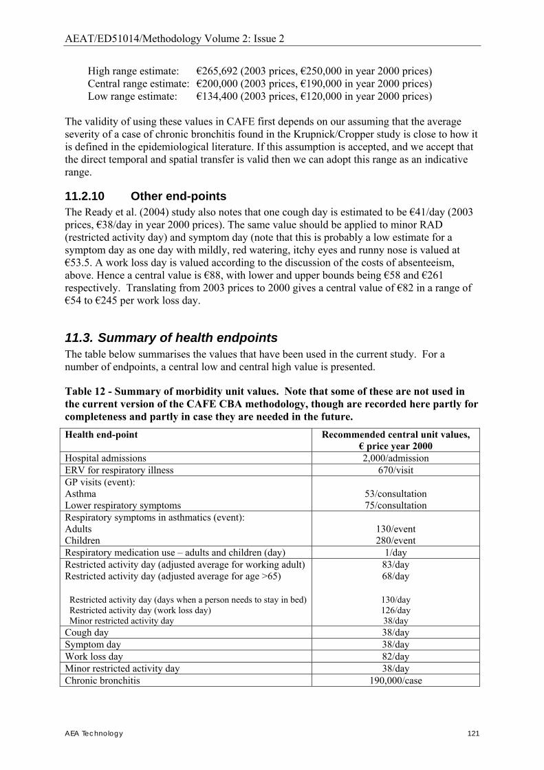
AEAT/ED51014/Methodology Volume 2: Issue 2
AEA Technology 121
High range estimate: �265,692 (2003 prices, �250,000 in year 2000 prices) Central range estimate: �200,000 (2003 prices, �190,000 in year 2000 prices) Low range estimate: �134,400 (2003 prices, �120,000 in year 2000 prices)
The validity of using these values in CAFE first depends on our assuming that the average severity of a case of chronic bronchitis found in the Krupnick/Cropper study is close to how it is defined in the epidemiological literature. If this assumption is accepted, and we accept that the direct temporal and spatial transfer is valid then we can adopt this range as an indicative range.
11.2.10 Other end-points The Ready et al. (2004) study also notes that one cough day is estimated to be �41/day (2003 prices, �38/day in year 2000 prices). The same value should be applied to minor RAD (restricted activity day) and symptom day (note that this is probably a low estimate for a symptom day as one day with mildly, red watering, itchy eyes and runny nose is valued at �53.5. A work loss day is valued according to the discussion of the costs of absenteeism, above. Hence a central value is �88, with lower and upper bounds being �58 and �261 respectively. Translating from 2003 prices to 2000 gives a central value of �82 in a range of �54 to �245 per work loss day.
11.3. Summary of health endpoints The table below summarises the values that have been used in the current study. For a number of endpoints, a central low and central high value is presented.
Table 12 - Summary of morbidity unit values. Note that some of these are not used in the current version of the CAFE CBA methodology, though are recorded here partly for completeness and partly in case they are needed in the future. Health end-point Recommended central unit values,
� price year 2000 Hospital admissions 2,000/admission ERV for respiratory illness 670/visit GP visits (event): Asthma Lower respiratory symptoms
53/consultation 75/consultation
Respiratory symptoms in asthmatics (event): Adults Children
130/event 280/event
Respiratory medication use � adults and children (day) 1/day Restricted activity day (adjusted average for working adult) Restricted activity day (adjusted average for age >65)
Restricted activity day (days when a person needs to stay in bed) Restricted activity day (work loss day) Minor restricted activity day
83/day 68/day
130/day 126/day 38/day
Cough day 38/day Symptom day 38/day Work loss day 82/day Minor restricted activity day 38/day Chronic bronchitis 190,000/case

AEAT/ED51014/Methodology Volume 2: Issue 2
122 AEA Technology
12. References Abbey DE, Petersen F, Mills PK, Beeson WL. (1993). Long-term ambient concentrations of
total suspended particulates, ozone and sulfur dioxide and respiratory symptoms in a non-smoking population. Arch Env Health; 48: 33-46.
Abbey DE, Hwang BL, Burchette RJ, Vancuren T, Mills PK. (1995a). Estimated long-term ambient concentrations of PM10 and development of respiratory symptoms in a nonsmoking population. Arch Env Health; 50: 139-152.
Abbey DE, Ostro BE, Petersen F, Burchette RJ (1995b). Chronic respiratory symptoms associated with estimated log-term ambient concentrations of fine particulates les than 2.5 micron in aerodynamic diameter (PM2.5) and other air pollutants. Journal of Exposure Analysis and Environmental Epidemiology; 5 (2): 137-159
Abbey, D.E. et al (1999) Long-term inhalable particles and other air pollutants related to mortality in nonsmokers. American journal of respiratory and critical care medicine, 159: 373-382.
Abrahamowicz M, Schopflocher T, Leffondré K, du Berger R, Krewski D. (2003). Flexible modeling of exposure-response relationship between long-term average levels of particulate air pollution and mortality in the American Cancer Society study. Journal of Toxicology and Environmental Health, Part A, 66: 1625-53.
Abt Associates (2000). The particulate-related health benefits of reducing power plant emissions. Prepared for EPA by Abt Associates Inc., 4800 Montgomery Lane, Bethesda, MD 20814-5341. http://www.abtassoc.com/reports/particulate-related.pdf
AEA Technology (1998) Economic Evaluation of Proposals for the Emission Ceilings Directive. Contract Report for DGXI of the European Commission.
Agee, M.D. and Crocker, T.D. (2001), �Smoking Parents� Valuations of Own and Children�s Health�, Paper presented at the Association of Environmental and Resource Economists conference, Bar Harbor, Maine, June 13-15, 2001.
Alberini A., Cropper, M. L., Krupnick A., and N. Simon (2004), �Does the Value of a Statistical Life Vary with Age and Health Status? Evidence from the U.S. and Canada,� Journal of Environmental Economics and Management, 48(1), 769-792
Anderson HR, Ponce de Leon A, Bland JM, Bower JS, Strachan DP (1996). Air pollution and daily mortality in London 1987-92. BMJ; 312: 665-9
APHEIS (Air Pollution and Health: A European Information System; 2004). Health impact assessment of air pollution and communication: Third Year Report, 2002-2003 (Apheis-3). Available at http://www.apheis.net/Apheis3NEW1.pdf; accessed November 2004.
APHEIS (Medina S., Plasència A., Artazcoz L. Quénel P., Katsouyanni K., Mücke H.-G., De Saeger E., Krzyzanowsky M., Schwartz J. and the contributing members of the APHEIS group) (2002). APHEIS Health Impact Assessment of Air Pollution in 26 European
AEAT/ED51014/Methodology Volume 2: Issue 2
AEA Technology 123
Cities. Second year report, 2000-2001. Institut de Veille Sanitaire, Saint-Maurice, France. (Apheis-2). � see also http://www.apheis.net/
Bell ML, McDermott A, Zeger SL, Samet JM, Dominici F. (2004). Ozone and short-term mortality in 95 US urban communities, 1987-2000. JAMA; 292:2372-8.
Bergendorff S (2003). Sickness absence in Europe � a comparative study. Fourth international research conference on social security. Available at http://www.issa.int/pdf/anvers03/topic5/2bergendorff.pdf; accessed November 2004
Bergendorff S, Berggren S, Cohen Birman M, Nyberg K, Palmer E, Skogman Thoursie P, Söderberg J (2002). Svensk sjukfrånvaro I ett europeiskt perspektiv. Riksförsäkringsverket: RFV analyserar 2002: 11.
Bliksvaer T, Helliesen A (1997). Sickness absence. A study of 11 LES countries. Presented at Luxembourg Employment Study Symposium, 1996.
Blomquist, G.C., Miller, T.R. and Levy, D.T. (1996), �Values of Risk Reduction Implied by Motorist Use of Protection Equipment�, Journal of Transport Economics and Policy, pp. 55-66.
Blomquist, G.C. (2003), �Self Protection and Averting Bahaviour, Values of Statistical Lives, and Benefit Cost Analysis of Environmental Policy�, National Center for Environmental Economics Working Paper No. 03-02, March.
Bobak M (2000): Outdoor air pollution, low birth weight and prematurity. Environ Health Perspect 108: 173-176.
Bobak M, Leon DA (1992): Air pollution and infant mortality in the Czech Republic, 1986-88. Lancet 340: 1010-1014.
Bobak M, Leon DA (1999): The effect of air pollution on infant mortality appears specific for respiratory causes in the postneonatal period. Epidemiology 10: 666-670.
Bobak M, Richards M, Wadsworth M (2001): Air pollution and birth weight in Britain in 1946. Epidemiology 111: 207-216.
Boezen M, Schouten J, Rijcken B, Vonk J, Gerritsen J, Zee S van der, Hoek G, Brunekreef B, Postma D (1998). Peak expiratory flow variability, bronchial responsiveness, and susceptibility to ambient air pollution in adults. American Journal of Respiratory & Critical Care Medicine, 158(6): 1848-1854.
Cameron, T.A. and J.R. DeShazo. 2004. An Empirical Model of Demand for Future Health States when Valuing Risk Mitigating Programs.
Carlin, P.S. and Sandy, R. (1991), �Estimating the Implicit Value of a Young Child�s Life,� Southern Economic Journal, Vol. 58, No. 1, pp. 186-202.
Carthy T., Chilton S., Dolan P., Jones-Lee M., Loomes G and A. Robinson (1999) Valuation of Benefits of Health and Safety Control. Report to UK Health & Safety Executive.
AEAT/ED51014/Methodology Volume 2: Issue 2
124 AEA Technology
CBI (1998) Missing out: 1998 absence and labour turnover survey. Confederation of British Industry, London.
COMEAP (Committee on the Medical Effects of Air Pollutants, 1998). The quantification of the effects of air pollution on health in the United Kingdom. London: HMSO
COMEAP Working paper 2002/9a (2003). Is there a threshold for the effect of ozone on health? Is there an effect on mortality and respiratory or circulatory hospital admissions? http://www.advisorybodies.doh.gov.uk/comeap/pdfs/june2002ozonethreshold.pdf; accessed November 2004. (NB: This is NOT an official publication of COMEAP or the UK Department of Health.)
Conceicao GMS, Miraglia SGEK, Kishi HS, Saldiva PHN, Singer JM (2001). Air pollution and child mortality: a time series study in Sao Paulo, Brazil. Environ Health Perspect; 109(suppl 3): 347-350.
Cropper, M.L., Aydede, S.K. and Portney, P.R. (1994), �Preferences for Life Saving Programs: How the Public Discounts Time and Age, Journal of Risk and Uncertainty, Vol. 8, No. 3, pp. 243-265.
Dab, W., Quenel, S.M.P., Le Moullec, Y., Le Tertre, A., Thelot, B., Monteil, C., Lameloise, P., Pirard, P., Momas, I., Ferry, R. and Festy, B. (1996). Short term respiratory health effects of ambient air pollution: results of the APHEA project in Paris. J Epidem Comm Health 50 (suppl 1): S42-46.
Day, B., Dubourg, R., Machado, F., Mourato, S., Navrud, S., Ready, R., Spanninks, F., and Rodriguez, M. (1999). �Benefits Transfer and the Economic Valuation of Environmental Damage in the European Union: With Special Reference to Health.� Final Report to the European Union DG XII. June 1999.
Declerq C, Macquet V (2000). [Short-term effects of ozone on respiratory health of children in Armentieres, North of France]. Rev Epidemiol Sante Publique; 48 Suppl 2: 2S37-43.
DEFRA (2004) Valuation of health benefits associated with reductions in air pollution. Final Report. May 2004. www.defra.gov.uk
Dickie, M. and Gerking, S. (2001), �Parents� Valuation of Latent Health Risks to their Children�, Working Paper presented at the US Environmental Protection Agency Workshop �Valuing of a Statistical Life: Assessing the State of the Art for Policy Applications�, November 6-7, Silver Spring, MD.
Dickie, M. and Ulery, V.L. (2001), �Valuing Health in the Household: Are Kids Worth More Than Parents?�, Paper presented at the Association of Environmental and Resource Economists 2001 Workshop: �Assessing and Managing Environmental and Public Health Risks�, June.
Dockery DW, Pope CA III (1994). Acute respiratory effects of particulate air pollution. Ann Rev Public Health; 15: 107-132.
Dockery, D.W., Speizer, F.E., Stram, D.O., Ware, J.H., Spengler, J.D. and Ferries, B.G. (1989). Effects of inhalable particles on respiratory health of children. Am Rev Respir Dis 139, 587-594.

AEAT/ED51014/Methodology Volume 2: Issue 2
AEA Technology 125
Dockery DW, Pope CA III, Xiping X, Spengler JD, Ware JH, Fay MA, Ferries BG Jr, Speizer FE (1993). An association between air pollution and mortality in six US cities. N. Engl J Med; 329(24): 1753-1759.
Dockins, C., Jenkins, R.R., Owens, N., Simon, N.B. and Wiggins, L.B. (2002), �Valuation of Childhood Risk Reduction: The Importance of Age, Risk Preferences and Perspective�, Risk Analysis, Vol. 22, No. 2.
Dusseldorp, A., Kruize, H., Brunekreef, B., Hofschreuder, P., de Meer, G. and van Oudvorst, A.B. (1995). Associations of PM10 and airborne iron with respiratory health of adults near a steel factory. Am J Respir Crit Care Med 152, 1932-9.
Eagan TML, Bakke PS, Eide GE, Gulsvik A (2002). Incidence of asthma and respiratory symptoms by sex, age and smoking in a community study. Eur Respir J; 19: 599-605.
EAHEAP (2000) Economic Appraisal of the Health Effects of Air Pollutants. For the Department of Health, London. http://www.doh.gov.uk/airpollution/ecomain.htm
EC DG ENV (2000) Papers on the valuation of mortality, from a workshop convened by the Commission in November 2000. http://www.europa.eu.int/comm/environment/enveco/others/value_of_life.htm
Environmental External Costs of Transport (2001). Editors Rainer Friedrich and Peter Bickel. Authors: Schmid, S., Bickel, P., Friedrich, R., Krewitt., Watkiss, P., Holland, M., et al. Published by Springer, 2001. ISBN 3-540-42223-4. Springer Verlag Berlin Heidelberg 2001.
ECRHS (1996). European Community Respiratory Health Survey: Variations in the prevalence of respiratory symptoms, self-reported asthma attacks, and use of asthma medication in the European Community Respiratory Health Survey (ECRHS). Eur Respir J; 9: 687-695.
ECRHS (European Community Respiratory Health Survey II Steering Committee, 2002). The European Community Respiratory Health Survey II. Eur Respir J; 20: 1071-1079.
European Lung White Book, 2003 (ed. Loddenkemper, R). The first comprehensive survey on respiratory health in Europe. European Respiratory Society, Lausanne, Switzerland.
ExternE (1995) DGXII (JOULE Programme) Externalities of Energy, ExternE Project, Report Number 2, Methodology. Prepared by ETSU and others.
ExternE (1999) DGXII (JOULE Programme) Externalities of Energy, ExternE Project, Report Number 7, Methodology: Update 1998. Holland, M.R. and Forster, D. (eds.).
Ezzati, M., Lopez, A., Rodgers, A., van der Hoorn, S., Murray, C.J.L. and the Comparative Risk Assessment Collaborating Group (2002) Selected major risk factors and global and regional burden of disease. The Lancet, 360, 1347-1360.
GBD (2000) See WHO. The World Health Report 2002. World Health Organization, Geneva.

AEAT/ED51014/Methodology Volume 2: Issue 2
126 AEA Technology
Gielen MH, van der Zee SC, van Wijnen JH, van Steen CJ, Brunekreef B (1997). Acute effects of summer air pollution on respiratory health of asthmatic children. Am J Respir Crit Care Med; 155: 2105-2108.
Glinianaia SV, Rankin J, Bell R, Pless-Mulloli T, Howel D. (2004a). Particulate air pollution and fetal health: a systematic review of the epidemiologic evidence. Epidemiology: 15: 36-45.
Glinianaia SV, Rankin J, Bell R, Pless-Mulloli T, Howel D. (2004b). Does particulate air pollution contribute to infant death? A systematic review. Environmental Health Perspectives; 112: 1365-1370.
Gryparis A, Forsberg B, Katsouyanni K, Analitis A, Touloumi G, Schwartz J, Samoli E, Medina S, Anderson HR, Niciu EM, Wichmann E, Kriz B, Kosnik M, Skorkovsky J, Vonk JM, Dortbudak Z. (2004). Acute effects of ozone on mortality from the �Air Pollution and Health: A European Approach� project. Am J Respir Crit Care Med;170:1080-1087.
Hajat S, Anderson HR, Atkinson RW and Haines A (2002). Effects of air pollution on general practitioner consultations for upper respiratory diseases in London. Occupational and Environmental Medicine 59:294-299
Hajat S, Haines A, Atkinson RW, Bremner SA, Anderson HR, Emberlin J (2001). Association between air pollution and daily consultations with general practitioners for allergic rhinitis in London, United Kingdom. Am J Epidemiol; 153: 704-14.
Hajat S, Haines A, Goubet S, Atkinson R, Anderson HR (1999). Association of air pollution with daily GP consultations for asthma and other lower respiratory conditions in London. Thorax 54: 597-605.
Hammitt, J.K. and J.T. Liu. 2004. Effects of Disease Type and Latency on the Value of Mortality Risk. Journal of Risk and Uncertainty 28: 73-95.
Hedley AJ, Wong CM, Thach TQ, Ma SLS, Lam TH, Anderson HR. (2002). Cardiorespiratory and all-cause mortality after restrictions on sulphur content of fuel in Hong Kong: an intervention study. Lancet. ; 360: 1646-1652.
Higgins, BG, Francis HC, Yates CJ, Warburton CJ, Fletcher AM, Reid JA, Pickering CAC, Woodcock AA (1995). Effects of air pollution on symptoms and peak expiratory flow measurements in subjects with obstructive airways disease. Thorax, 50: 149-155.
Hiltermann, TJN, Stolk J, Zee SC van der, Brunekreef B, de Bruijne CR, Fischer PH, Ameling CB, Sterk PJ, Hiemstra PS, Bree L van (1998). Asthma severity and susceptibility to air pollution. European Respiratory Journal, 11: 686-693.
Hoek G, Brunekreef B (1995). Effect of photochemical air pollution on acute respiratory symptoms in children. Am J Respir Crit Care Med; 151: 27-32.
Hoek, G, Brunekreef, B, Goldbohm, S, Fischer, P, van den Brandt, PA. (2002) The association between mortality and indicators of traffic-related air pollution in a Dutch cohort study. Lancet, 360: 1203-1209.
AEAT/ED51014/Methodology Volume 2: Issue 2
AEA Technology 127
Holland, M.R., Forster, D. and King, K. (1999) Cost-Benefit Analysis for the Protocol to Abate Acidification, Eutrophication and Ground Level Ozone in Europe. Report Number: Air and Energy 133, Ministry of Housing, Spatial Planning and Environment (MVROM), Directorate Air and Energy, ipc 640, P.O. Box 30945, 2500 GX The Hague, The Netherlands.
Hurd M. D. and K. McGarry (1997) The Predictive validity of subjective probabilities of survival. National Bureau of Economic Research. Working Paper no. 6193. September 1997.
Hurley, J.F., Holland, M. R., Markandya, A., Miller, B.G., Anderson, H.R., Ayres, J.G., Donnan, P.T., Harrison, R.M., King, K., Stedman, J. and Stevenson, K. (2000) Towards assessing and costing the health impacts of ambient particulate air pollution in the UK. Contract report for the UK Department of Health.
ICP/MM (2003) Mapping Manual Revision. United Nations Economic Commission for Europe, ICP Mapping and Modelling. http://www.oekodata.com/icpmapping/html/manual.html
IGCB (2001) An economic analysis to inform the review of the air quality strategy for particles. Second Report of the Interdepartmental Group on Costs and Benefits. Department of the Environment, Food and Rural Affairs in partnership with the Scottish Executive, The National Assembly for Wales and the Department of the Environment for Northern Ireland.
IIASA (2002) A methodology to estimate changes in statistical life expectancy due to the control of particulate matter air pollution. International Institute for Applied Systems Analysis, Laxenburg, Austria.
IOM and AEA Technology (2003) Quantifying the Health Impacts of Pollutants Emitted in Central Scotland. P830. Report for the Scottish Executive by: The Institute of Occupational Medicine and AEA Technology plc. February 2003.
ISAAC Committee (1998). The International Study of Asthma and Allergies in Childhood Steering Committee. Worldwide variations in the prevalence of asthma symptoms: the international study of asthma and allergies in childhood (ISAAC). Eur Respir J; 12: 315-335.
Janson C, Anto J, Burney P, Chinn S, de Marco R, Heinrich J, Jarvis D, Kuenzli N, Leynaert B, Luczynska C, Neukirch F, Svanes C, Sunyer J, Wjst M, on behalf of the European Community Respiratory Health Survey II (2001). The European Community Respiratory Health Survey: what are the main results so far? Eur Respir J; 18: 598-611.
Jenkins, R.R., Owens, N. and Wiggins, L.B. (2001), �Valuing Reduced Risks to Children: The Case of Bicycle Safety Helmets�, Contemporary Economic Policy, Vol. 19, No. 4, pp. 397-408.
Jerrett M, Burnett R, Ma R, Thurston G, Newbold B, Finkelstein N, Shi Y, Krewski D, Thun M. (2004). Air Pollution and mortality in Los Angeles (abstract). Health Effects Institute Annual Conference.
AEAT/ED51014/Methodology Volume 2: Issue 2
128 AEA Technology
Jones-Lee (1991) Altruism and the Value of Other People's Safety Journal of Risk and Uncertainty Vol. 4, pp213-219
Jones-Lee, M W, 1992. "Paternalistic Altruism and the Value of Statistical Life. Economic Journal, vol. 102(127), pages 80-90.
Jones-Lee, M., Hammerton, M. and Philips, P. (1985) The value of safety: results of a national sample survey. Economic Journal, 95, 49-72.
Joyce, T.J., Grossman, M. and Goldman, F. (1989), �An Assessment of the Benefits of Air Pollution Control: The Case of Infant Health�, Journal of Urban Economics, Vol. 25, pp. 32-51.
Just J, Segala C, Sahraoui F, Priol G, Grimfeld A, Neukirch F. (2002). Short-term health effects of particulate and photochemical air pollution in asthmatic children. European Respiratory Journal, 20: 899-906.
Kaiser R, Romieu I, Medina S, Schwartz J, Krzyzanowski M, Künzli N. (2004). Air pollution attributable postneonatal infant mortality in US metropolitan areas: A risk assessment study. Environmental Health: A global access science source 3. http://www.ehjournal.net/content/3/1/4
Krewski D, Burnett RT, Goldberg MS, Hoover K, Siemiatycki J, Abrahamowicz M, White WH (2000). Re-analysis of the Harvard Six-cities study and the American Cancer Society Study of air pollution and mortality. Cambridge, MA: Health Effects Institute. Available at http://www.healtheffects.org/pubs-special.htm
Krupnick A and M. Cropper (1992) The Effect of Information on Health Risk Valuation, Journal of Risk and Uncertainty Vol. 5, 29-48
Krupnick A.J., Harrington W., Ostro B. (1990). Ambient ozone and acute health effects: Evidence from daily data. J. Environ Econ Manage 18, 1-18.
Krupnick, A., Alberini, A., Cropper M., Simon N., O�Brien B., Goeree R., and M. Heintzelman (2002), �Age, Health, and the Willingness to Pay for Mortality Risk Reductions: A Contingent Valuation Survey of Ontario Residents,� Journal of Risk and Uncertainty, 24, 161-186.
Krzyzanowski M, Jedrychowski W, Wysocki M, (1986). Factors associated with the change in ventilatory function and the development of chronic obstructive pulmonary disease in a 13-year follow-up of the Cracow study. Am Rev Respir Dis; 134: 1011-1019.
Künzli N, Kaiser R, Medina S, Studnicka M, Chanel O, Herry M, Horak F, Puybonnieux-Texier V, Quénel P, Schneider J, Seetaler R, Vergnaud J-C, Sommer H. (2000). Public health impact of outdoor and traffic-related air pollution: a European assessment. Lancet, 356: 795-801.
Le Tetre A, Medina S, Samoli E, Forsberg B, Michelozzi P, Boumghar A et al. (2002). Short-term effects of particulate air pollution on cardiovascular diseases in eight European cities. J Epidemiology and Community Health 56: 773-779
AEAT/ED51014/Methodology Volume 2: Issue 2
AEA Technology 129
Levy JI, Carrothers TJ, Tuomisto JT, Hammitt JK, Evans JS. (2001). Assessing the public health benefits of reduced ozone concentrations. Environ Health Perspect 109:1215-26.
Lewis, P.A. and Charny, M. (1989), Which of Two Individuals Do You Treat When Only Their Ages Are Different And You Can�t Treat Both?, Journal of Medical Ethics, Vol. 15, No. 1, pp. 28-34.
Liu, J.T, Hammitt, J.K., Wang, J.D. and Liu, J.L. (2000), �Mothers Willingness To Pay For Her Own And Her Child�s Health: A Contingent Valuation Study in Taiwan, Health Economics, Vol. 9, pp. 319-326.
Maddison D (1997) Valuing the Morbidity Effects of Air Pollution, CSERGE, UCL, London, mimeo.
McDonnell WF, Abby DE, Nishino N, Lebowitz MD (1999). Long-term ambient concentration and the incidence of asthma in non-smoking adults: the AHSMOG study. Environ Res. 80(2, part 1): 110-121
Miller BG, Hurley JF. (2003). Life table methods for quantitative impact assessments in chronic mortality. J Epidemiol. Community Health, 57: 200-206.
Mount, T., Weng, W., Schulze, W. and Chestnut, L. (2001), �Automobile Safety and the value of Statistical Life in the Family: Valuing Reduced Risks for Children, Adults and the Elderly�, Paper presented at the 2001 Association of Environmental and Resource Economists Workshop, Bar Harbor, Maine, June 13-15, 2001.
Navrud, S. (2001): "Valuing Health Impacts from Air Pollution in Europe", Environmental and Resource Economics, 20(4):305-329.).
Netten, A. and Curtis, L. (2000) Unit costs of Health and Social Care 2000. Personal Social Services Research Unit (PSSRU). http://www.pssru.ac.uk/index.htm .
Neukirch F, Segala C, Le Moullec Y, Korobaeff M, Aubier M (1998). Short-term effects of low-level winter pollution on respiratory health of asthmatic adults. Archives of Environmental Health, 53: 320-328.
ORNL/ RFF (1994). Estimating Externalities of the Coal Fuel Cycle. report 3 on the external costs and benefits of fuel cycles. A study by the US Department of Energy and the Commission of the European Communities. Prepared by Oak Ridge National Laboratory and Resources for the Future. McGraw Hill.
Ostro B.D. (1987). Air pollution and morbidity revisited: A specification test. J Environ Econ Manage 14, 87-98.
Ostro B.D. and Rothschild S. (1989). Air pollution and acute respiratory morbidity: An observational study of multiple pollutants. Environ Res 50, 238-247.
Ostro BD, Lipsett MJ, Mann JK, Krupnick A, Harrington W (1993). Air pollution and respiratory morbidity among adults in Southern California. Am J Epidemiol; 137: 691-700.
AEAT/ED51014/Methodology Volume 2: Issue 2
130 AEA Technology
Ostro B, Chestnut L, Vichit-Vadakan N, Laixuthai A (1999). The impact of particulate matter on daily mortality in Bangkok, Thailand. Air & Waste Manage Assoc; 49: PM-100-107.
Otterstrom T., Gynther L. and Vesa P. (1998) The willingness to pay for better air quality, Ekono Energy Ltd.
Pearce (1992) Pearce, D., Bann, C. and Georgiou, S.: The Social Costs of Fuel Cycles. A report to the UK Department of Energy. The Centre for Economic and Social Research into the Global Environment, (CSERGE), University College London and University of East Anglia: 1992.
Pearce (1998) Valuing Statistical Lives Planejamento e Politicas Publicas, December 1998, 18, 69 � 118.
Peters A, Goldstein IF, Beyer U, Franke K, Heinrich J, Dockery DW, Spengler JD, Wichmann HE (1996). Acute health effects of exposure to high levels of air pollution in Eastern Europe. Am J Epidemiol; 144: 570-81.
Pilkington, A. et al (1997) Health effects of heavy metals, dioxins, and other atmospheric organic pollutants. In ExternE (1999a) Chapter 9.
Ponce de Leon A., Anderson H.R., Bland J.M., Strachan D.P. and Bower J. (1996). Effects of air pollution on daily hospital admissions for respiratory disease in London between 1987-88 and 1991-92. J Epidem Comm Health 50 (suppl 1): S63-70.
Pope C.A. and Dockery D.W. (1992). Acute health effects of PM10 pollution on symptomatic and asymptomatic children. Am Rev Respir Dis 145, 1123-1126.
Pope C.A. III, Thun M.J., Namboodiri M.M., Dockery D.W., Evans J.S., Speizer F.E. and Heath C.W. Jr. (1995). Particulate air pollution as predictor of mortality in a prospective study of US adults. Am J Resp Crit Care Med 151: 669-674.
Pope, CA III, Burnett RT, Thun MJ, Calle EE, Krewski D, Ito K, Thurston GD (2002). Lung cancer, cardiopulmonary mortality, and long-term exposure to fine particulate air pollution. Journal of the American medical association, 287: 1132 - 1141.
Portney PR, Mullahy J (1986). Urban air quality and acute respiratory illness. Journal of Urban Economics; 20: 21-38.
Rabl, 2001 to be added Rabl A 2002. �Relation Between Life Expectancy and Probability of Dying.� Report Centre d�Energétique, Ecole des Mines, 60 boul. St.-Michel, F-75272 Paris. Available from author at [email protected]. Need to change year
Rabl, A. (2003) Interpretation of air pollution mortality: Number of deaths or years of life lost? Journal of the Air & Waste Management Association; Vol.53(1), 41-50 (2003).
Ready, R., Navrud S., Day B, Dubourg R., Machado F., Mourato S., Spanninks F., and M. X. V. Rodriquez. (2004) Benefit Transfer in Europe: How Reliable Are Transfers Across Countries? Environmental & Resource Economics 29: 67-82
AEAT/ED51014/Methodology Volume 2: Issue 2
AEA Technology 131
Roemer W, Hoek G, Brunekreef B (1993). Effect of ambient winter air pollution on respiratory health of children with chronic respiratory symptoms. Am Rev Respir Dis; 147: 118-124.
Roemer W, Clench-Aas J, Englert N, Hoek G, Katsouyanni K, Pekkanen J, Brunekreef B (1999). Inhomogeneity in response to air pollution in European children (PEACE project). Occup Environ Med; 56: 86-92.
Roemer W, Hoek G, Brunekreef B (2000). Pollution effects on asthmatic children in Europe, the PEACE study. Clinical and Experimental Allergy; 30: 1067-1075.
Scappechi P. (2003) Valuation Differences Between Adults and Children. Paper presented at: Workshop on the Valuation of Children�s Health, National Policies Division, OECD Environment Directorate11-12 September 2003
Schwartz J. and Morris R. (1995) Air pollution and hospital admissions for cardiovascular disease in Detroit, Michigan. Am J Epidem 142, 23-35. Am J Epidem 137, 701-705.
Schwartz J. (1997). Air pollution and hospital admissions for cardiovascular disease in Tucson. Epidemiology; 8:371-7.
Segala, C. et al (1998). Short-term effect of winter air pollution on respiratory health of asthmatic children in Paris. European Respiratory Journal. 11: 677-685.
Spix C, Heinrich J, Dockery D, Schwartz J, Volksch G, Schwinkowski K (1993). Air pollution and daily mortality in Erfurt, East Germany, 1980-1989. Env Health Pers; 101: 518-519.
Stieb DM, Smith-Doiron M, Brook JR, Burnett RT, Dann T, Mamedov A, Chen Y. (2002). Air pollution and disability days in Toronto: Results from the National Population Health Survey.
Sunyer J., Castellsague J., Saez M., Tobias A. and Anto J.M. (1996) Air pollution and mortality in Barcelona. J Epidem Comm Health 50 (suppl 1): S76-S80.
Tamburlini, G. (2003) Oveview of the risk differences between Adults and Children. Paper presented at: Workshop on the Valuation of Children�s Health, National Policies Division, OECD Environment Directorate11-12 September 2003
Tiitanen P, Timonen KL, Ruskanen JJ, Mirme A, Pekkanen J (1999). Fine particulate air pollution, resuspended road dust and respiratory health among symptomatic children. Eur Respir J; 13: 266-273.
Timonen KL, Pekkanen J (1997). Air pollution and respiratory health among children with asthmatic or cough symptoms. Am J Resp Crit Care Med; 156: 546-552.
Touloumi G., Samoli E. and Katsouyanni K. (1996). Daily mortality and �winter type� air pollution in Athens, Greece - a time series analysis within the APHEA project. J Epidem Comm Health 50 (suppl 1): S47-S51.
AEAT/ED51014/Methodology Volume 2: Issue 2
132 AEA Technology
USEPA (1997) The benefits and costs of the Clean Air Act: 1970 to 1990. United States Environmental Protection Agency, Office of Air and Radiation/Office of Policy, Washington D.C..
USEPA/Abt Associates, 2003 to be added
Verhoeff AP, Hoek G, Schwartz J, van Wijnen JH (1996). Air pollution and daily mortality in Amsterdam. Epidemiology; 7: 225-230.
Viscusi, W.K., Magat, W.A. and Huber, J. (1991) Pricing Environmental Health Risks: Survey Assessments of Risk-Risk and Risk-Dollar Tradeoffs for Chronic Bronchitis. Journal of Environmental Economics and Management, Vol. 21, No. 1 (July 1991), pp. 32-51.
von Klot S, Wolke G, Tuch T, Heinrich J, Dockery DW, Schwartz J, Kreyling WG, Wichmann HE, Peters A. (2002). Increased asthma medication use in association with ambient fine and ultrafine particles. European Respiratory Journal, 20: 691-702.
Ward DJ, Ayres JG (2004). Particulate air pollution and panel studies in children: a systematic review. Occup Environ Med. 61(4): e13
Watkiss, P, Baggot, S, Bush T, Cross, S, Goodwin, J, Hunt, A, Hurley, F, Holland M, Stedman, J (2005). Evaluation of Air Quality Strategy (EPES 0203/1). Published by DEFRA, January 2005. AEA Technology Environment, Metroeconomica, and the Institute of Occupational Medicine. http://www.defra.gov.uk/environment/airquality/strategy/evaluation/index.htm
Whittemore, A.S. and Korn, E.L. (1980). Asthma and air pollution in the Los Angeles area. Am J Public Health 70, 687-696.
WHO (2000) Quantification of the health effects of exposure to air pollution. WHO, European Centre for Environment and Health, Bonn. http://www.euro.who.int/document/e74256.pdf.
WHO (2002) World health report 2002. Geneva, World Health Organization, 2002.
WHO (2003) Heath aspects of air pollution with particulate matter, ozone and nitrogen dioxide, Report on a WHO Working Group, Bonn, Germany, 13-15 January 2003. World Health Organisation: Available at http://www.euro.who.int/document/e79097.pdf ; accessed November 2004.
WHO (2004) Health aspects of air pollution �answers to follow-up questions from CAFE. Report on a WHO Working Group meeting, Bonn, Germany, 15-16 January 2004. World Health Organisation: Available at http://www.euro.who.int/document/e82790.pdf ; accessed November 2004.
WHO (2004); prepared by Anderson HR, Atkinson RW, Peacock JL, Marston L, Konstantinou K. Meta-analysis of time-series studies and panel studies of particulate matter (PM) and ozone (O3). Report of a WHO task group. World Health Organization. (http://www.euro.who.int/document/e82792.pdf; accessed November 2004
AEAT/ED51014/Methodology Volume 2: Issue 2
AEA Technology 133
WHO (2004, pending) The Effects of Air Pollution on Children�s Health and Development: a review of the evidence. Executive Summary available at http://www.euro.who.int/document/EEHC/execsum.pdf; accessed November 2004.
Woodruff TJ, Grillo J, Schoendorf KC: The relationship between selected causes of postneonatal infant mortality and particulate air pollution in the United States. Environ Health Perspect 1997, 105: 608-612. http://ehp.niehs.nih.gov/members/1997/105-6/woodruff.html
Wordley J., Walters S. and Ayres J.G. (1997) Short term variations in hospital admissions and mortality and particulate air pollution. Occup Environ Med 54, 108-116.
Zee, S van der. et al (1999). Acute effects of urban air pollution on respiratory health of children with and without chronic respiratory symptoms. Occupational and Environmental Medicine, 56: 802-812.
Zee S van der, Hoek G, Boezen HM, Schouten JP, Wijnen JH van, Brunekreef B (2000). Acute effects of urban air pollution on respiratory health of 50-70 yr old adults. Eur Respir J 15, 700-709