Embed Size (px)
Citation preview

Centre for Sustainable Electricity and Distributed Generation
Cost Benefit Methodology for Optimal Design of Offshore Transmission
Systems
Predrag Djapic and Goran Strbac
July 2008
FUNDED BY BERR
URN 08/1144

[blank]
Cost Benefit Methodology for Optimal Design of Offshore Transmission Systems
Table of Contents
Executive Summary ..................................................................................................... 9 1. Background, Overall Aims and Scope of Work ................................................... 16 2. Cost Benefit Analysis Methodology ..................................................................... 18 3. Offshore Transmission Network Topologies ........................................................ 20
3.1 Design Principles of Offshore Transmission Systems ............................... 21 4. Evaluation of EEC and Losses .............................................................................. 23
4.1 Wind Power Characteristics ....................................................................... 23 4.2 Evaluation of Capacity Outage Probability Tables for Offshore Transmission Systems ........................................................................................... 26
4.2.1 Two-state Elements ................................................................................ 26 4.2.2 Characterisation of Wind Power Output for Reliability Evaluations .... 27
4.3 Evaluation of Expected Energy Curtailed ................................................. 28 4.4 Cost of Expected Energy Curtailed ........................................................... 29 4.5 Evaluation of Losses .................................................................................. 29
5. Reactive Compensation ......................................................................................... 31 6. Evaluation of Costs of Assets and Corrective (Post Fault) Maintenance ............. 34 7. Minimum Capacity Factor – X Factor .................................................................. 36 8. Sensitivity Analysis – Robustness of Design ........................................................ 40
8.1 Platform Design ......................................................................................... 40 8.1.1 Number of Transformers ....................................................................... 40 8.1.2 Maximum Rating of a Single Transformer Connection ........................ 41
8.2 Cable System Design ................................................................................. 43 8.2.1 Number of Cables .................................................................................. 43 8.2.2 Cable Redundancy Analysis .................................................................. 45 8.2.3 Voltage Level ......................................................................................... 46
8.3 Onshore Circuit Design ............................................................................. 47 8.4 Onshore Substation Design ........................................................................ 49 8.5 Offshore Transmission System Design for GT .......................................... 50 8.6 HVDC VSC Design ................................................................................... 50
9. Impact of Planned Outages of Offshore Infrastructure for Wind Based Generation 52
9.1 Background ................................................................................................ 52 9.2 Methodology for Inclusion of Impact of Planned Outages on Design of Offshore Transmission Equipment ....................................................................... 52 9.3 Design of Offshore and Onshore Substation ............................................. 54
9.3.1 Two Transformers per Offshore and Onshore Substation ..................... 54 9.3.2 Single Transformer per Offshore Platform ............................................ 55 9.3.3 Single Transformer per Onshore Substation .......................................... 57
9.4 Design of submarine cables ....................................................................... 58 9.5 Design of Onshore Circuit ......................................................................... 59
Page 3 of 86

Cost Benefit Methodology for Optimal Design of Offshore Transmission Systems
9.5.1 Design of Overhead Line 132 kV .......................................................... 59 9.5.2 Design of Overhead Line 220 kV .......................................................... 65 9.5.3 Design of Onshore Underground Cable System .................................... 66
10. Rating Limits of a Single Circuit – Impact on Frequency Control ................ 67 10.1 Rating Limit of a Single Converter Block in HVDC Applications ........... 67 10.2 Rating Limit of a Single Circuit ................................................................ 69
11. An Example ................................................................................................... 71 12. Key Findings .................................................................................................. 75 13. References ...................................................................................................... 80 14. Appendix – Equipments and Cost Data ......................................................... 81
14.1 Update of Equipment and Cost Data ......................................................... 84 14.1.1 New Cost Data ................................................................................... 84 14.1.2 Further CBA dataset for Inclusion of Preventive Maintenance ......... 85
Page 4 of 86

Cost Benefit Methodology for Optimal Design of Offshore Transmission Systems
List of Tables
Table 1 – Results for 132kV onshore overhead lines (with generic maintenance of OH lines) .................................................................................. 12
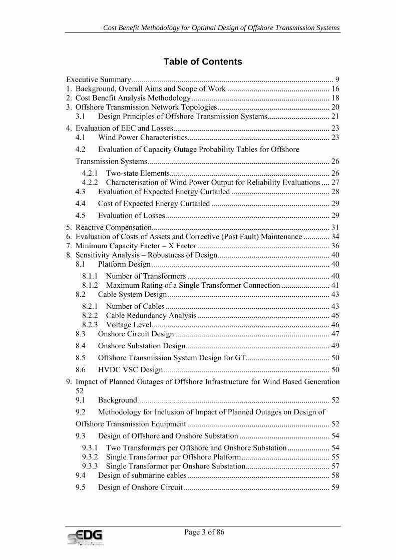
Table 2 – Results for 220kV onshore overhead lines (with generic maintenance of OH lines) .................................................................................. 13
Table 3 – Characteristics of wind generation profiles ............................................... 24 Table 4 – Capacity outage probability table for two-state elements. ......................... 26 Table 5 – General form of capacity outage probability table with N states. ............. 27 Table 6 – Maximum active power output of wind farm in MW ................................ 32 Table 7 – Required offshore and onshore compensation in MVAr to
maintain the maximum active power transfer capabilities of the offshore transmission system (conditions given in Table 6) ............................. 32
Table 8 – Voltage at the offshore side of cable (busbar 2) for the conditions given in Table 6 ................................................................................................. 33
Table 9 – Wind farms capacity (MW) that change cable optimum configuration (change from one cable rating to the next and change in number of cables used). ..................................................................................... 36
Table 10 – X factor for cables ................................................................................... 37 Table 11 – Wind farm capacity (MW) that change transformer size solution. ......... 37 Table 12 – X factor for transformers ......................................................................... 38 Table 13 – Minimum capacity factors – X factors (%) for shared
connections ........................................................................................................ 39 Table 14 – Mean time to repair in months ................................................................. 40 Table 15 – Break-even parameters shown in bold. The first figure is
associated with diversified wind profile, second represent the average value, while the third refers to non-diversified wind profile ............................. 41
Table 16 – Break-even parameters shown in bold. The values below break-even favour a single cable while those above favour a two cable design. ................................................................................................................ 44
Table 17 – Break-even values of MTTR are shown in bold ...................................... 44 Table 18 – Break-even MTTR of cables ................................................................... 45 Table 19 – Break-even energy costs .......................................................................... 45 Table 20 – Break-even MTTR (months) shown in bold ............................................ 46 Table 21 – Break-even MTTR of cables ................................................................... 46 Table 22 – Total cost (m£) of 132 and 220 kV configurations. ................................. 47 Table 23 – Results for 132 kV onshore overhead lines: number, type and
rating in MW of circuits ..................................................................................... 48 Table 24 – Parameters for Markov model of overhead lines ..................................... 49 Table 25 – Wind farm ratings for which a breakeven costs are obtained (for
wind farm ratings above 500 MW only diversified wind profile, wind profile index 2, are used) ................................................................................... 49
Table 26 – Additional cost due to maintenance for case of wind farm of 250 MW .................................................................................................................... 54
Table 27 – Additional cost due to maintenance for case of wind farm of 480 MW .................................................................................................................... 55
Table 28 – Additional cost and benefit of installing two transformers for wind farm of 60 MW ......................................................................................... 56
Page 5 of 86

Cost Benefit Methodology for Optimal Design of Offshore Transmission Systems
Table 29 – Additional cost and benefit of installing two transformers for wind farm of 90 MW ......................................................................................... 56
Table 30 – Additional cost and benefit of installing two transformers for wind farm of 120 MW ....................................................................................... 56
Table 31 – Additional cost and benefit of installing two transformers at onshore substation. Offshore substation consists of 2 transformers of 60 MW each. ...................................................................................................... 57
Table 32 – Additional cost and benefit of installing two transformers at onshore substation. Offshore substation consists of 2 transformers of 90 MW each. ...................................................................................................... 57
Table 33 – Additional cost and benefit of installing two transformers at onshore substation. Offshore substation consists of 2 transformers of 120 MW each. .................................................................................................... 58
Table 34 – Additional cost and benefit of installing two transformers at onshore substation. Offshore substation consists of 2 transformers of 150 MW each. .................................................................................................... 58
Table 35 – Results for 132kV onshore overhead lines (with generic maintenance of OH lines) .................................................................................. 59
Table 36 – Additional cost and benefit of different onshore overhead circuit of length of 1km. Rating of wind farm is 150 MW, availability 95%. Offshore substation consists of 2 transformers of 75 MW each. Submarine cable 132 kV 1x500 mm2 50 km is maintenance free. .................... 59
Table 37 – Additional cost and benefit of different onshore overhead circuit of length of 10km. Rating of wind farm is 150 MW, availability 95%. Offshore substation consists of 2 transformers of 75 MW each. Submarine cable 132 kV 1x500 mm2 50 km is maintenance free. .................... 60
Table 38 – Additional cost and benefit of different onshore overhead circuit of length of 25km. Rating of wind farm is 150 MW, availability 95%. Offshore substation consists of 2 transformers of 75 MW each. Submarine cable 132 kV 1x500 mm2 50 km is maintenance free. .................... 60
Table 39 – Additional cost and benefit of different onshore overhead circuit of length of 50km. Rating of wind farm is 150 MW, availability 95%. Offshore substation consists of 2 transformers of 75 MW each. Submarine cable 132 kV 1x500 mm2 50 km is maintenance free. .................... 61
Table 40 – Additional cost and benefit of different onshore overhead circuit of length of 1km. Rating of wind farm is 250 MW, availability 95%. Offshore substation consists of 2 transformers of 120 MW each. Submarine cable 132 kV 2x500 mm2 50 km is maintenance free. .................... 61
Table 41 – Additional cost and benefit of different onshore overhead circuit of length of 10km. Rating of wind farm is 250 MW, availability 95%. Offshore substation consists of 2 transformers of 120 MW each. Submarine cable 132 kV 2x500 mm2 50 km is maintenance free. .................... 62
Table 42 – Additional cost and benefit of different onshore overhead circuit of length of 25km. Rating of wind farm is 250 MW, availability 95%. Offshore substation consists of 2 transformers of 120 MW each. Submarine cable 132 kV 2x500 mm2 50 km is maintenance free. .................... 62
Table 43 – Additional cost and benefit of different onshore overhead circuit of length of 50km. Rating of wind farm is 250 MW, availability 95%.
Page 6 of 86

Cost Benefit Methodology for Optimal Design of Offshore Transmission Systems
Offshore substation consists of 2 transformers of 120 MW each. Submarine cable 132 kV 2x500 mm2 50 km is maintenance free. .................... 63
Table 44 – Additional cost and benefit of different onshore overhead circuit of length of 1km. Rating of wind farm is 400 MW, availability 95%. Offshore substation consists of 2 transformers of 200 MW each. Submarine cable 132 kV 2x800 mm2 50 km is maintenance free. .................... 63
Table 45 – Additional cost and benefit of different onshore overhead circuit of length of 10km. Rating of wind farm is 400 MW, availability 95%. Offshore substation consists of 2 transformers of 200 MW each. Submarine cable 132 kV 2x800 mm2 50 km is maintenance free. .................... 64
Table 46 – Additional cost and benefit of different onshore overhead circuit of length of 25km. Rating of wind farm is 400 MW, availability 95%. Offshore substation consists of 2 transformers of 200 MW each. Submarine cable 132 kV 2x800 mm2 50 km is maintenance free. .................... 64
Table 47 – Additional cost and benefit of different onshore overhead circuit of length of 50km. Rating of wind farm is 400 MW, availability 95%. Offshore substation consists of 2 transformers of 200 MW each. Submarine cable 132 kV 2x800 mm2 50 km is maintenance free. .................... 65
Table 48 – Results for 220kV onshore overhead lines (with generic maintenance of OH lines) .................................................................................. 65
Table 49 – Additional cost and benefit of different onshore overhead circuit 220 kV of length of 25km. Rating of wind farm is 1000 MW, availability 95%. Planned outage duration is 10 hours per overhead circuit. Onshore substation is not considered. ................................................... 66
Table 50 – Constraints imposed by “infrequent” loss of 1000MW ........................... 68 Table 51 – Probability that the output of a wind farm of a given capacity is
above 1000MW level ......................................................................................... 68 Table 52 – Characteristics of response providing units ............................................. 69 Table 53 – Additional annual response costs ............................................................. 70 Table 54 – HVDC singe and double circuit costs (1500MW) ................................... 70 Table 55 – Cable losses. ............................................................................................ 72 Table 56 – Transformers and cables losses. .............................................................. 72 Table 57 – Transformers and cables reliability parameters. ...................................... 72 Table 58 – Capacity outage probability table. ........................................................... 73 Table 59 – EEC cost. ................................................................................................. 73 Table 60 – Total cost. ................................................................................................ 74 Table 61 – Results for 132kV onshore overhead lines (with generic
maintenance of OH lines) .................................................................................. 76 Table 62 – Results for 220kV onshore overhead lines (with generic
maintenance of OH lines) .................................................................................. 76 Table 63 – HVAC cables cost. ................................................................................... 82 Table 64 – HVDC cables cost. ................................................................................... 82 Table 65 – Electrical parameters of HVAC cables .................................................... 82 Table 66 – Electrical parameters of HVDC cables .................................................... 83 Table 67 – Reliability parameters .............................................................................. 83 Table 68 – Cost of ‘small’ transformers .................................................................... 83 Table 69 – AC submarine cables costs ...................................................................... 84 Table 70 – AC underground cables costs .................................................................. 84 Table 71 – Base cost of 132 /33 kV transformers ...................................................... 84
Page 7 of 86

Cost Benefit Methodology for Optimal Design of Offshore Transmission Systems
List of Figures
Figure 1 – Schematic diagram offshore transmission system considered ................... 9 Figure 2 – Concept of cost-benefit analysis ............................................................... 18 Figure 3 – Comparison of various transmission networks solutions ......................... 19 Figure 4 – An example of a directly connected offshore network. ............................ 20 Figure 5 – An example of a shared connection. ........................................................ 20 Figure 6 – An example of the use of HVDC technology ........................................... 21 Figure 7 – A platform design ..................................................................................... 21 Figure 8 – Direct connection design .......................................................................... 22 Figure 9 – Shared connection design ......................................................................... 22 Figure 10 – A design principle (where the arrow can represent either the
offshore platform or undersea cable network) ................................................... 22 Figure 11 – Normalized wind output ......................................................................... 24 Figure 12 – Wind generation duration profiles. ......................................................... 25 Figure 13 – Calculation of constrained wind energy. ................................................ 25 Figure 14 – Constrained wind energy. ....................................................................... 26 Figure 15 – Determining model for intermittent generation. ..................................... 28 Figure 16 – Network configuration for calculation of cable capability. P1
and P3 active power at offshore and onshore GEP, respectively. ...................... 31 Figure 17 – Platform capacity of 60 MW .................................................................. 42 Figure 18 – Platform capacity of 90 MW .................................................................. 42 Figure 19 – Platform capacity of 120 MW ................................................................ 43 Figure 20 – Overhead lines reliability model ............................................................ 48 Figure 21 – Total costs for various solutions for offshore network ........................... 51 Figure 22 – Load duration curve for diversified wind summer profile during
preventive maintenance period (June – August) ................................................ 53 Figure 23 – Curtailed energy factor during preventive maintenance outage ............. 53
List of Abbreviations
AC Alternating Current
DC Direct Current
BERR Department for Business, Enterprise and Regulatory Reform
EEC Expected Energy Constrained
GB Great Britain
HVDC High Voltage Direct Current
Ofgem Office of Gas and Electricity Markets
OTEG Offshore Transmission Experts Group
ROCs Renewable Obligation Certificates
SGT Super Grid Transformer
SQSS GB Security and Quality of Supply Standard
Page 8 of 86

Page 9 of 86
Cost Benefit Methodology for Optimal Design of Offshore Transmission Systems
Executive Summary This document summarises the results of a cost-benefit analysis (CBA) based methodology developed to determine the optimal design of offshore transmission grid to connect offshore wind farms and gas turbines to onshore electricity networks. Although work was conducted in two phases this report presents the combined results of both of these activities. The CBA methodology implemented was used for the development of the new GB Security and Quality of Supply Standard (SQSS) for Offshore Transmission Networks, as a part of the activities carried out by the GBSQSS sub-group of OTEG. The recommendations for an offshore standard made on the basis of this cost-benefit analysis have since been consulted on and the majority of the initial recommendations for the basis of an offshore security standard were agreed by BERR.1
It was assumed that the offshore transmission system, for which a schematic diagram is presented in Figure 1, will operate at 132kV or above. Furthermore, such systems will be composed of a (i) cable undersea network and (ii) single or multiple offshore platforms with transformers for HVAC transmission or converters for HVDC together with associated switching and compensation equipment and (iii) on-shore circuit and (iv) the on-shore substation that connects the offshore system to the onshore one.
Offshore plant
Offshore cables
ShorelineOffshore Platform
OnshoreGrid
Onshore circuit
Onshore substation
Offshore Transmission Network
Figure 1 – Schematic diagram offshore transmission system considered
The cost benefit approach developed and applied to determine the optimal design of offshore networks is conceptually identical to the one used in the planning and design of onshore systems2. A balancing exercise between the following two broad categories of costs is carried out to determine the optimal network design:
1 The Government’s decision is available on the BERR website at: http://www.berr.gov.uk/files/file38855.pdf 2 The network design according to the GBSQSS for on shore networks is centred around two sets of considerations (i) peak security (defined through “planned transfer” and “interconnection allowance”) followed by (ii) a CBA that can be used to justify investment over an above those driven by security consideration. Unlike conventional generation, wind power makes a very limited contribution to securing peak demand and hence peak security considerations in network design for wind power are not practically relevant (and are hence ignored in this analysis), as the network investment will be

Page 10 of 86
Cost Benefit Methodology for Optimal Design of Offshore Transmission Systems
• cost of offshore transmission system investment, that is composed of:
o costs of undersea cable network o cost of platform with associated equipment (transformers, reactive
compensation and switchgear) o cost of onshore circuits and substation and reactive compensation o capitalised cost of corrective maintenance and
• capitalised cost of expected constrained energy due to preventive and corrective maintenance and losses over the period of the asset life.
Based on evaluating the above two cost components for a spectrum of feasible offshore transmission system configurations with different levels of redundancy, we have identified optimal designs for undersea cable network and offshore platforms (including compensation both onshore and offshore), for a range of wind farms with ratings up to 1500 MW and for a range of offshore gas turbines (GTs) with ratings up to 200 MW and various distances ranging from 25 km to 100 km. Furthermore, optimal designs of onshore circuits with length ranging from 1 to 50 km and onshore substations have been identified.
This analysis suggests that economically efficient offshore networks for wind energy should be designed with no redundancy, due to the significantly higher cost of undersea cables when compared to overhead lines (with a factor of about 20), the absence of demand offshore, the relatively low load factor of wind generation (40%) and the low capacity (security) value of offshore wind generation that can be relied upon to secure onshore demand. Hence, the suggested designs tend to be radial rather than interconnected, although in some cases there will be benefits of sharing connections among wind farms that are located geographically close to each other. Hence, for offshore wind farms, all four offshore network sections (offshore platform, offshore cable connection, onshore network and onshore substation that makes the connection to the onshore grid), are all design with no redundancy. In case of GT with capacities greater than 100 MW (but less than 200MW), minimum rating of individual transformers in multiple transformer offshore substations should provide (N-1) redundancy, while all other three sections of the offshore grid would not have any redundancy.
Although the optimal network design for wind farms requires no redundancy, the security of the connection can be very significant, particularly for larger wind farms. This is driven by the power transfer limitations of AC undersea cables3. Currently used 132kV AC cables can carry up to about 250MW while modern 400kV overhead lines can carry over 2000MW over longer distances4. For example, the connection of a 600 MW wind farm offshore will require the installation of at least three 132 kV cables due to the limited power transfer capability of undersea cables. Hence, a loss of one of those cables will result in an expected energy curtailment that is only
driven by CBA (cost of constraints and losses versus cost of investment, considering both normal operation and maintenance (corrective and preventive). Hence, conceptually the design of on and offshore networks follow the same principles. 3 Application of HVDC technologies for this purpose and distances involved may still not be competitive. 4 Note that the application of 400 kV AC is not competitive due to single-core based design and very significant reactive compensation requirement.

Page 11 of 86
Cost Benefit Methodology for Optimal Design of Offshore Transmission Systems
around 8 % of the total energy production that would be expected to be achieved before the fault is repaired. Given the relatively small number of expected cable faults over the lifetime of the scheme, the expected energy constrained (EEC) due to outages of offshore network components (for wind costed at £75/MWh and including the value of ROCs) will be relatively small and cannot justify the building of redundant offshore networks.
Although no consideration has been given to the financial compensation arrangements for partial losses of transmission system access (or the relevant offshore transmission charging arrangements), it is important to stress that there is no fundamental difference in the design philosophy between on and offshore systems5.
Furthermore, our previous assessment6 indicates that after all Round 2 projects are connected, the expected cost of offshore wind energy that will be constrained due to failures on the network is between £10.8m and £13.1m per annum, even under conservative assumptions regarding network repair times. When compared with post BETTA constraint costs - that are in the region of £100m - costs of offshore wind driven constraints would make a relatively modest contribution to the overall constraint costs.
It is however important to stress that the methodology developed (and consequent recommendations for the planning standard) is based on the assumption that the wind energy curtailed associated with every network design (and the corresponding costs) represents a long term average (expected) value of energy curtailed over the life time of the project. Expected values of energy curtailed would be approximately achieved from operating a large number of offshore schemes over a long period of time. In practice, there will be a potentially significant variation in the energy curtailed associated with individual wind farms, as these may experience a higher or lower number of outages than the expected long term average would suggest, and hence higher or lower levels of curtailed energy than the long term average. Clearly, the risks of achieving higher values of energy curtailed than the long term average value, on a specific project (particularly small projects that would be connected to a single cable), may be sufficiently higher than that used in the study, and if considered in isolation, it might warrant a network design with higher levels of redundancy than optimal (and higher, inefficient, corresponding investment costs).
Specific recommendations The detailed cost-benefit analysis suggested that the design of offshore network systems could be separated into four main sections:
• the offshore platform (i.e. the AC transformer circuits and HVDC converters on the offshore platform);
5 Balancing the cost of investment against the cost of losses and constraints is the basis of economically efficient design of both on and off shore networks. In other words, the cost benefit used for offshore network design determines the economically efficient design of offshore networks and is conceptually identical to that used onshore although the detailed solutions are different due to different cost structure of the network assets and the fundamental characteristics of generation. 6 P Djapic, G Strbac, Grid Integration Options for Offshore Wind Farms, December 2006, www.berr.gov.uk/files/file36129.pdf

Cost Benefit Methodology for Optimal Design of Offshore Transmission Systems
• the offshore cable network (i.e. the transmission cable circuits linking the onshore network and the offshore platform);
• the onshore circuit if necessary • the onshore substation if necessary
Each of the four sections can be considered separately for single and multiple generation plants connections. However, the potential for coordination of preventative maintenance activities across offshore assets has been considered.
It should be noted from the results presented that each of the key input parameters has been tested to find the value at which the conclusion changes. A number of the key items of the input data to the cost benefit analysis have been tested (average repair times, cost of wind or gas turbines energy curtailed, etc.) to investigate at what level these would change the design recommendations of the cost benefit analysis. A comprehensive set of more than 35,000 sensitivity studies was performed to propose the optimal design and to demonstrate the robustness of the recommendations made.
Offshore transmission network design for wind farms The following recommendations for offshore transmission system for wind farms are drawn:
• Minimum number of submarine cables with no redundancy. The total capacity of cables can be lower than the maximum export capacity of wind farms connected (see X factor in table below)
• Maximum rating of single transformer substation for offshore platform is 90MW. Minimum rating for multi-transformer substations is 50% of the wind farm rating and there is no impact of preventive maintenance
• Design of 132 kV overhead lines for wind farms to 400 MW is given in Table 1. For wind farms up to 1100 MW it is double circuit and above that is two double circuits. Design of 220 kV overhead lines are given in Table 2. Design of onshore underground cables will follow design of offshore subsea cables. However, there might be benefit of connecting two subsea cables to one onshore underground cable.
• Maximum rating of single transformer substation for onshore substation is 120-180MW
Table 1 – Results for 132kV onshore overhead lines (with generic maintenance of OH lines)
Length (km) Wind farm capacity (MW)
150 250 400
1 SC DC DC
10 SC SC/DC DC
25 SC SC DC
50 SC SC SC/DC
• SC – Single circuit • DC – Double circuit
Page 12 of 86
Cost Benefit Methodology for Optimal Design of Offshore Transmission Systems
Table 2 – Results for 220kV onshore overhead lines (with generic maintenance of OH lines)
Length (km)
Wind farm capacity (MW)
400 600 800 1000 1060
≤2 DC DC DC DC DC
≤4 SC DC DC DC DC
≤8 SC SC DC DC DC
≤25 SC SC SC DC DC
≤50 SC SC SC SC DC
As the diversity of wind power output was considered to potentially have an impact on the design of cable network, two extreme wind profiles are used:
• a non-diversified profile, characteristic for relatively small wind farms occupying relatively small geographical areas, and
• a diversified profile, characteristic for relatively large wind farms occupying relatively large areas. In this case, due to the dispersed locations of the wind generators, statistically there is a relatively low probability that full output of all individual wind generators will be available at any given time.
Offshore platform
The quantitative assessments demonstrated that offshore platform capacity should be about 95% of the maximum export capacity of the wind farm connected (for AC solutions). Furthermore, for wind farms with a capacity of 90MW or greater, following an outage (planned or unplanned) of any offshore platform transformer, there should be, at a minimum, 50% of the installed platform transformer capacity remaining. Significant benefits of the flexibility have been observed. It is important to stress however, it is sufficient that the switching supply from one to the other circuit (in case of a fault) is manual (rather than automatic) provided that it is completed within the time frame that is on average significantly shorter than the average repair times of transformers and cables (6 and 2 months respectively)
DC Offshore platforms are built with no redundancy.
Offshore Cable Network
For cable networks, the total optimal capacity installed can be lower than the maximum export capacity of the wind farm connected, due to the cost of installing offshore transmission assets to full capacity (X factor in table below). For the non-diversified wind profile (appropriate for relatively small wind farms, occupying small geographical areas) the installed network capacity should be above 95% of the maximum output of the wind farm, while in the case of a diversified wind profile (appropriate for relatively large wind farms occupying relatively large areas) the installed network capacity should be above 90% of the maximum output of the wind
Page 13 of 86

Cost Benefit Methodology for Optimal Design of Offshore Transmission Systems
farm. In cases where this value requires an additional cable to be installed, consideration should be given to installation of network capacity below 95% for a non-diversified profile and below 90% for diversified profiles. The optimal values of the X factor will be a function of the distance as shown in the table below.
X factor (%) Cable length (km)
Wind farm profile
Condition - Increase in 25 50 75 100
Non-diversified wind profile
Cable rating >95Number of cables >91 >88 >86 >84
Diversified wind profile
Cable rating >90Number of cables >85 >82 >79 >77
For wind farms connected through HVDC technology, following an outage (planned or unplanned) of any single offshore platform DC converter module, the loss of power infeed is proposed not to exceed the existing onshore Normal Infeed Loss Risk (1000MW). However, it would be economically efficient to connect wind farms of 1500MW (maximum considered) to a single offshore transmission circuits.
Onshore overhead lines and cables design
Onshore overhead lines are preferable solution due to high cost of onshore cables. Design of 132 kV overhead lines for wind farms up to 400 MW is given in Table 1. For wind farms between 400MW and 1100 MW it was found that a double circuit overhead line would be optimal, while for capacities of 1100MW and above that the design should be based on two double circuits. Design of 220 kV overhead lines are given in Table 2. Note that a single size conductor for 220 kV overhead lines was considered.
If cables are to be used, the design should follow one developed for offshore (the obtained data revealed that underground cables are significantly more expensive than equivalent undersea cables). However, there might be a benefit of connecting two subsea cables to a system of single-core onshore underground cable.
Onshore substation design
For wind farms of 120MW or greater, there should be a minimum of 2 transformers installed onshore, with the capacity such that following a planned or fault outage of a transformer there is a minimum of 50% of installed capacity remaining. This is driven by planned maintenance requirements. Offshore transmission network design for GTs
The recommendations for the optimal design of offshore transmission networks for GTs are as follows:
• Design of offshore substations for GT capacity up to 100 MW a single transformer offshore substation and for capacity greater than 100 MW
Page 14 of 86

Page 15 of 86
Cost Benefit Methodology for Optimal Design of Offshore Transmission Systems
minimum rating of individual transformers in multiple transformer offshore substations with full (N-1) redundancy7
• Design of submarine link: single cable • Design of onshore link: single circuit • Design of onshore substation: single transformer
The impact of preventive maintenance is also analysed including coordination of maintenance of different network assets. The analysis demonstrated that design of offshore infrastructure for GT generation was not impacted by preventive maintenance outages.
7 In the analysis conducted only single rating of GT of 100MW was used.

Page 16 of 86
Cost Benefit Methodology for Optimal Design of Offshore Transmission Systems
1. Background, Overall Aims and Scope of Work The Ofgem scoping document on ‘Offshore electricity transmission’ published in April 20068 identified issues that required further consideration in order to implement an offshore electricity transmission regime. The scoping document noted that DTI and Ofgem would take this work forward in conjunction with industry through a working group, OTEG (Offshore Transmission Expert Group).
OTEG then established a sub group (‘the GBSQSS sub-group’) to undertake review work to assist Ofgem/DTI decisions relating to offshore transmission system security requirements. The purpose of the GBSQSS sub-group was to assist OTEG by completing a review of the current GBSQSS and consequently considering:
a) whether it is appropriate to apply to the present onshore standard to offshore transmission networks
b) if amendments are needed to extend the GBSQSS offshore; and
c) the range of options that exist for alternative security standards for offshore transmission networks.
The BERR Centre for Sustainable Electricity and Distributed Generation provided analytical and numerical support in performing studies, analysing results and providing recommendations to the GBSQSS sub-group. This work was based on a cost benefit methodology and software tools that were developed to provide quantitative cost estimates of alternative configurations and levels of redundancy. The aim of the cost benefit analysis was to determine an optimum economic and technical solution for offshore transmission networks, taking into account the key driving factors that were likely to have an impact on the design of the offshore transmission systems.
The aim of the analysis has been to assess the minimum cost solution and then to justify any reinforcement above that value. The results that are presented along with this note illustrate the total cost for each solution, which includes the capital cost of the assets to be installed, cost of system losses, value of estimated energy curtailed, cost of reactive compensation and cost of maintenance over the lifetime of the assets.
Wind farms of up to 1500 MW of installed capacity and up to 100 km from connection point at the onshore grid are considered in this analysis. The network models created were populated with data from a set that was collated from suppliers, developers and the three onshore transmission licensees.
It should be noted from the results presented that each of the key input parameters has been tested to find the value at which the conclusion changes. These demonstrate the robustness of the recommendations made.
Although it was recognised that the Grid Code conditions will also be reviewed as part of the project to introduce an offshore transmission regulatory regime, these 8 The Scoping Documents is available on the Ofgem website at: http://www.ofgem.gov.uk/Pages/MoreInformation.aspx?docid=3&refer=Networks/Trans/Offshore/ConsultationDecisionsResponses

Cost Benefit Methodology for Optimal Design of Offshore Transmission Systems
were considered to be outside of the scope of the GBSQSS review. The studies carried out in this report confirmed that the voltage fluctuation considerations and reactive power requirements can be decoupled from the design of the main offshore infrastructure. No specific consideration has been given to the security of connection on the distribution network should offshore transmission networks connect to the DNO network.
The study has been performed in two phases: phase one included design of offshore platform and offshore cable system under normal and forced outage conditions while phase two adds studies on offshore GTs, onshore assets of offshore transmission systems and impact of planned maintenance.
Page 17 of 86
Cost Benefit Methodology for Optimal Design of Offshore Transmission Systems
2. Cost Benefit Analysis Methodology A cost benefit analysis approach was used to determine the optimum capacity of offshore transmission systems (transformers on the offshore platforms and undersea cable networks). This analysis identified the key parameters which impact on the proposed solution and considered a range of possible values to demonstrate the robustness of proposals against a range of input data.
This analysis has considered all wind farm connections anticipated to be connected to an offshore transmission network from Rounds 1 and 2, along with all characteristics of the assets to be installed in the network that will have an impact on the outcome of the analysis.
Generic offshore wind farms were modelled to include the consideration of single and shared, AC and DC connections. The objective of this analysis was to determine the optimum economic and technical solution for an offshore network connecting to the onshore electricity grid system.
In this analysis, it is assumed that offshore transmission networks will be cable circuits for the connection from the offshore high voltage platform to the first substation that the circuit reaches onshore.
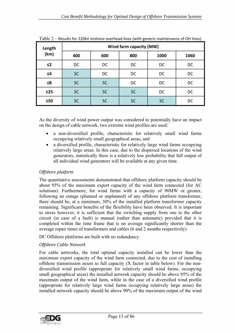
Figure 2 shows the concept of cost-benefit analysis. Cost
Optimal network Network Capacity and Redundancy
Cost of constrained wind energy and losses
Investment and Maintenance costs
Total cost
Figure 2 – Concept of cost-benefit analysis The developed cost benefit analysis is employed to find optimal tradeoffs between the following two broad categories of costs:
• cost of offshore transmission system investment, that is composed of: o costs of undersea cable network o cost of platform with associated equipment (transformers, reactive
compensation and switchgear) o cost of onshore circuits and substation and reactive compensation
Page 18 of 86
Page 19 of 86
Cost Benefit Methodology for Optimal Design of Offshore Transmission Systems
o capitalised cost of corrective maintenance and • capitalised cost of expected constrained energy due to preventive and
corrective maintenance and losses over the period of the asset life. Based on evaluating the above two cost components for a spectrum of feasible offshore transmission system configurations with different levels of redundancy, we have identified optimal designs for undersea cable networks and offshore platforms (including compensation both onshore and offshore), for a range of wind farms with ratings up to 1500MW and various distances ranging from 25km to 100km.
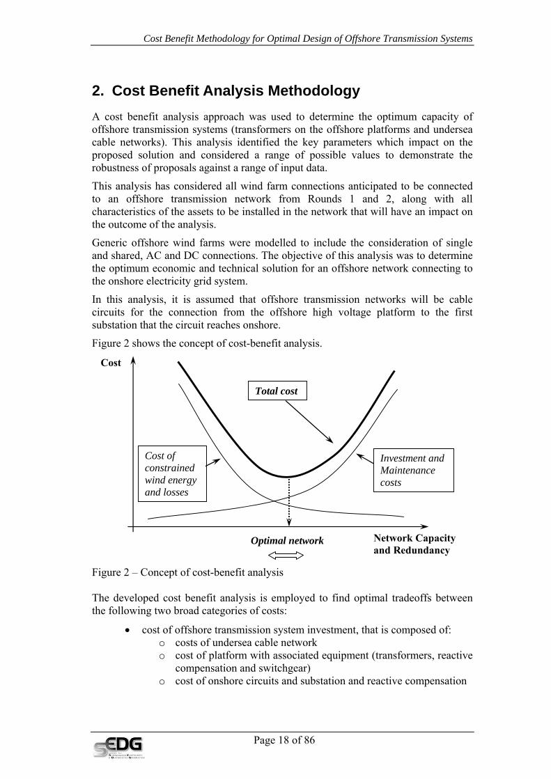
Figure 3 shows cost comparison of various transmission network solutions.
0
50
100
150
1 2 1 2 1 2 1 2 1 2 1 2 1 2 1 2 1 2 1 2 1 2 1 2 1 2 1 2 1 2 1 2 1 2 1 2 1 2 1 2
200
250
300
201 201 201 201 293 319 293 293 553 553 553 553 589 589 637 722 748 863 748 863
800 800 800 800 630 800 630 630 1000 1000 1000 1000 1400 1400 1600 2000 630 800 630 800
3 c. 3 c. 3 c. 3 c. 2 c. 2 c. 2 c. 1 c. 1 c. 1 c. 1 c. 1 c. 1 c. 1 c. 1 c.
300 325 350 200 300 MW t. 325 350 275 300 325 350 550 600 MW t. 550 MW t. 600 MW t.
2 t. 3 t. 2 t. 2 t. 1 t. 1 t.
132 kV 220 kV 400 kV 150 kV 300 kV
AC DC
Cos
t (m
£)
Platform & plant cost (m£) Cables cost (m£) MVArs cost (m£) EEC cost (m£) Losses cost (m£) Mainenance cost (m£)
Test 1 Wind farms capacity (MW) 600 MW Cable length (km) 100 km
Technology Voltage (kV) Number of transformersTransformer rating (MWNumber of cables Cable size (mm²) Cable capability (MW) Wind profile index
Data
Wind profile index Cable capability (MW) Cable size (mm2) Number of cables Transformers rating (MVA)Number of transformers Voltage (kV) Technology
Cables cost (m£)
Wind farm size Distance to shore
EEC cost (m£)
Platform & plant cost (m£)
Y axis cost (m£)
X axis label description
Losses cost (m£)
Corrective maintenance cost (m£)
Compensation cost (m£)
Legend
Figure 3 – Comparison of various transmission networks solutions The information necessary for the calculations of all cost components is available on the GBSQSS sub-group webpage9. The platform and plant costs are generic and consist of fixed costs for foundation, float out and erect and variable costs for topsides with plant costs being linearly dependent on the number and rating of the transformers. The compensation plant is costed separately. The cost of cables, supply, lay and bury are also generic and for a specific cable rating are given per km.
9 http://www.dti.gov.uk/energy/sources/renewables/policy/offshore-transmission/offshore-transmission-experts-group/page31187.html

Cost Benefit Methodology for Optimal Design of Offshore Transmission Systems
3. Offshore Transmission Network Topologies As discussed above, offshore transmission systems are composed of two main components:
• the offshore platform (i.e. the AC transformer circuits and HVDC converters on the offshore platform); and
• the offshore cable network (i.e. the transmission cable circuits linking the onshore network and the offshore platform).
A number of different offshore network configurations are analysed. Figure 4 shows a layout of a directly connected offshore wind farm via a single platform, while Figure 5 shows an example of a shared or joint connection.
33 kV 220kV 220 kV
Onshore network
Wind farm electrical system
Platform
Shoreline
Undersea cable
Figure 4 – An example of a directly connected offshore network.
3x2x3x500 mm2
33 kV
132 kV
shoreline
500 MW 500 MW 500 MW
132 kV
220 kV
4x360 MVA
4x360 MVA
4x3x1000 mm2
220 kV
400 kV
Onshore grid
3 x 2x240/(2x120) MVA
Master platform
Figure 5 – An example of a shared connection. Interconnected offshore network topology is not investigated. To get an example of HVDC transmission network connections one should replace in AC networks the connection to the onshore by HVDC components (see Figure 6).
Page 20 of 86
Page 21 of 86
Cost Benefit Methodology for Optimal Design of Offshore Transmission Systems
shoreline
500 MW 500 MW 500 MW
132 kV
33 kV
±300 kV
132 kV
On-shore transmission network
±300 kV
132 kV
33 kV
132 kV
33 kV
AC DC
AC DC
AC DC
DC AC
DC AC
DC AC
275 or 400 kV
3 x 600 MW
3 x 600 MW
500 MW 500 MW 500 MW
(4x3) x 500 mm2(4x3) x 500 mm2
(4x3) x 500 mm2 10 km 10 km
10 km
40 km
4x173 MW
4x173 MW
4x173 MW
3 x 2 x 2 x 800 mm2
6 x 361 MVA (359 MW)
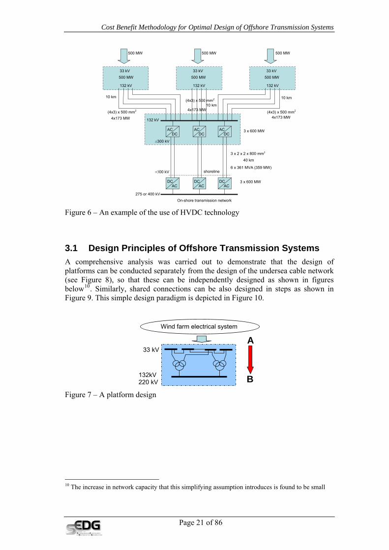
Figure 6 – An example of the use of HVDC technology
3.1 Design Principles of Offshore Transmission Systems A comprehensive analysis was carried out to demonstrate that the design of platforms can be conducted separately from the design of the undersea cable network (see Figure 8), so that these can be independently designed as shown in figures below10. Similarly, shared connections can be also designed in steps as shown in Figure 9. This simple design paradigm is depicted in Figure 10.
33 kV
132kV 220 kV B
AWind farm electrical system
Figure 7 – A platform design
10 The increase in network capacity that this simplifying assumption introduces is found to be small

Cost Benefit Methodology for Optimal Design of Offshore Transmission Systems
132kV/220 kV
33 kV
Onshore network
132 kV/220kV
Wind farm electrical system
B
A
Figure 8 – Direct connection design
132 kV
33 kV
400 kV
132 kV
Onshore network
400 kV
132 kV
33 kV
132 kV
33 kV
A
A
B
B
Figure 9 – Shared connection design
BA
Figure 10 – A design principle (where the arrow can represent either the offshore platform or undersea cable network) This feature considerably simplifies the analysis and the form of the standard.
Page 22 of 86

Cost Benefit Methodology for Optimal Design of Offshore Transmission Systems
4. Evaluation of EEC and Losses The volume of energy losses and expected energy may be curtailed due to unavailability of transformers and cables of offshore transmission networks. The methodology for this evaluation is based on the assumption that wind energy curtailed associated with every network design (and the corresponding costs) represents a long-term average (expected) value of energy curtailed. In practice, the expected value of energy curtailed can be approximately achieved from operating a large number of offshore schemes over a relatively long period of time. In practice, there will be potentially significant variations in the energy curtailed associated with individual wind farms, as they may experience higher or lower number of outages than the expected long-term average, and hence higher or lower levels of curtailed energy than the long-term average. Clearly, the risks of achieving higher values of energy curtailed than the long-term average value on a specific project may be sufficiently higher than that used in the study that it might warrant a network design with higher levels of redundancy (and higher corresponding investment costs).
Although no consideration has been given to the financial compensation arrangements for loss of transmission system access (or the relevant offshore transmission charging arrangements), it is important to bear in mind that the methodology developed and the corresponding network design are based on the expected long term average values of wind energy curtailed. In practice, this can be achieved from averaging the curtailed energy across a significant number similar of the wind farms.
We consider two 40% load factor normalised wind farms output profiles. We use two extreme wind generation output profiles, diversified and non-diversified, to assess network requirements. For large wind farms, or groups of wind farms, spread across a very wide geographical area the diversity effects may be significant (“diverse” wind out profile may be appropriate), while small wind farms covering a small geographical area will be characterized by lower diversity (“non-diverse” wind output profiles may be appropriate). However, no specific wind data was available to make firm recommendations regarding the application of diverse or non-diverse wind profiles in relation to specific areas that find farms may occupy.
Although it is not anticipated that the differences in offshore transmission system design between diversified and non-diversified will be very significant, these have however been routinely assessed to ensure robustness of any recommendations made.
In the following sections the evaluation methodology is described, while the date used is provided in Section 14, while an example application using the developed methodology and data is given in Section 11.
4.1 Wind Power Characteristics The output of a wind farm is fundamental to the output of the cost benefit analysis due to a need to establish the volume of energy curtailed during various outages of components of individual offshore transmission system designs. The features of the wind output profiles can be statistically assessed from the frequency distribution of
Page 23 of 86
Cost Benefit Methodology for Optimal Design of Offshore Transmission Systems
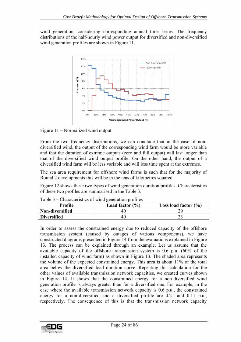
wind generation, considering corresponding annual time series. The frequency distributions of the half-hourly wind power output for diversified and non-diversified wind generation profiles are shown in Figure 11.
Figure 11 – Normalized wind output From the two frequency distributions, we can conclude that in the case of non-diversified wind, the output of the corresponding wind farm would be more variable and that the duration of extreme outputs (zero and full output) will last longer than that of the diversified wind output profile. On the other hand, the output of a diversified wind farm will be less variable and will less time spent at the extremes.
The sea area requirement for offshore wind farms is such that for the majority of Round 2 developments this will be in the tens of kilometres squared.
Figure 12 shows these two types of wind generation duration profiles. Characteristics of these two profiles are summarised in the Table 3.
Table 3 – Characteristics of wind generation profiles Profile Load factor (%) Loss load factor (%)
Non-diversified 40 29 Diversified 40 23 In order to assess the constrained energy due to reduced capacity of the offshore transmission system (caused by outages of various components), we have constructed diagrams presented in Figure 14 from the evaluations explained in Figure 13. The process can be explained through an example. Let us assume that the available capacity of the offshore transmission system is 0.6 p.u. (60% of the installed capacity of wind farm) as shown in Figure 13. The shaded area represents the volume of the expected constrained energy. This area is about 11% of the total area below the diversified load duration curve. Repeating this calculation for the other values of available transmission network capacities, we created curves shown in Figure 14. It shows that the constrained energy for a non-diversified wind generation profile is always greater than for a diversified one. For example, in the case where the available transmission network capacity is 0.6 p.u., the constrained energy for a non-diversified and a diversified profile are 0.21 and 0.11 p.u., respectively. The consequence of this is that the transmission network capacity
Page 24 of 86

Cost Benefit Methodology for Optimal Design of Offshore Transmission Systems
requirements for non-diversified wind outputs will tend to be greater than for diversified wind outputs (in relative terms).
00.10.20.30.40.50.60.70.80.9
1
0 1344 2688 4032 5376 6720 8064
Duration (h)
Pow
er (p
.u.)
Load factor: 0.4
Diversified profile
Non-diversified profile
Figure 12 – Wind generation duration profiles.
00.10.20.30.40.50.60.70.80.9
1
0 1344 2688 4032 5376 6720 8064
Duration (h)
Pow
er (p
.u.)
Load factor: 0.4
Diversified profile
Non-diversified profile
Available capacity
Constrained energy
Figure 13 – Calculation of constrained wind energy.
Page 25 of 86

Cost Benefit Methodology for Optimal Design of Offshore Transmission Systems
00.10.20.30.40.50.60.70.80.9
1
0 0.1 0.2 0.3 0.4 0.5 0.6 0.7 0.8 0.9 1
Power (p.u.)
Cons
train
ed E
nerg
y (p
.u.) Load factor: 0.4
Diversified profile
Non-diversified profile
Figure 14 – Constrained wind energy.
4.2 Evaluation of Capacity Outage Probability Tables for Offshore Transmission Systems
The reliability performance of the offshore transmission system is evaluated using analytical reliability techniques based on the concept of the Capacity Outage Probability Tables. The capacity outage probability tables for the offshore transmission system are derived from two-state representations of individual network components (in service or in outage).
4.2.1 Two-state Elements The basic model for assessing the reliability of two-state elements is generally through the use of capacity outage probability tables. The theory relating to these can be found in various reliability texts (for example, Billinton and Allan 1992 and 1996). In order to form the capacity outage probability table for two-state elements, the capacity (C) and associated critical period availability (A) should be known for that element. The capacity outage probability table, for that case, is shown in Table 4.
Table 4 – Capacity outage probability table for two-state elements.
State Capacity Probability 1 C A 2 0 1-A
A general form of the capacity outage probability table for a system composed of a number of two-states elements is shown in Table 5.
Page 26 of 86

Cost Benefit Methodology for Optimal Design of Offshore Transmission Systems
Table 5 – General form of capacity outage probability table with N states. State Capacity Probability
1 C1 p1
2 C2 p2
… ... … N CN pN
Note: Ci > Cj for i < j and Σpi = 1 It is assumed that capacity outage probability tables are known for each network element. The capacity outage probability table for a group of elements (such a system of transformers and cables connected in parallel or in series) is formed by convolving the tables of the individual elements together. For example, if two capacity outage probability tables are convolved together, the resulting capacity outage probability table is derived by combining each state of the first table with each state of table second table. Therefore, a new table has the characteristics shown in Algorithm 1. After creating the new table, states with the same capacity are combined as shown in Algorithm 2.
Algorithm 1 – Convolution of two capacity outage probability tables A and B • the theoretical number of states in the new table is the product of numbers of
states in table A and in table B, • the capacity quantities in the new table for parallel elements are simply the
sum of the equivalent states in tables A and B and for elements in series are the minimum of the equivalent states in tables A and B, whilst the probabilities are the products of the equivalent states (see equation (1)),
• states with zero probability are omitted.
BABA
BjAik
BjAi
BjAik
NNNNkNjNi
ppp
CCCC
C
⋅====
⋅=⎩⎨⎧ +
=
,..1,..1,..1 where
seriesin elementsfor ),,min(parallelin elementsfor ,
(1)
Algorithm 2 – Combining states of the capacity outage probability table After creating a new table, the states are sorted in descending order according to "capacity-in" column, and states with the same capacity are combined. The capacity of a combined state is the same as the capacities of each individual state, where probability of the combined state is the sum of individual probabilities. The new capacity outage probability table has the same structure as the one shown in Table 5.
4.2.2 Characterisation of Wind Power Output for Reliability Evaluations
Various wind generation output levels (between zero and maximum output) are represented as a multi-state generator characterized by its available capacities and associated probabilities. A practical approach to form such output probability tables is to characterise the variable as a time-varying parameter with its chronological behaviour fully represented. A schematic illustration of a generation pattern is shown
Page 27 of 86
Cost Benefit Methodology for Optimal Design of Offshore Transmission Systems
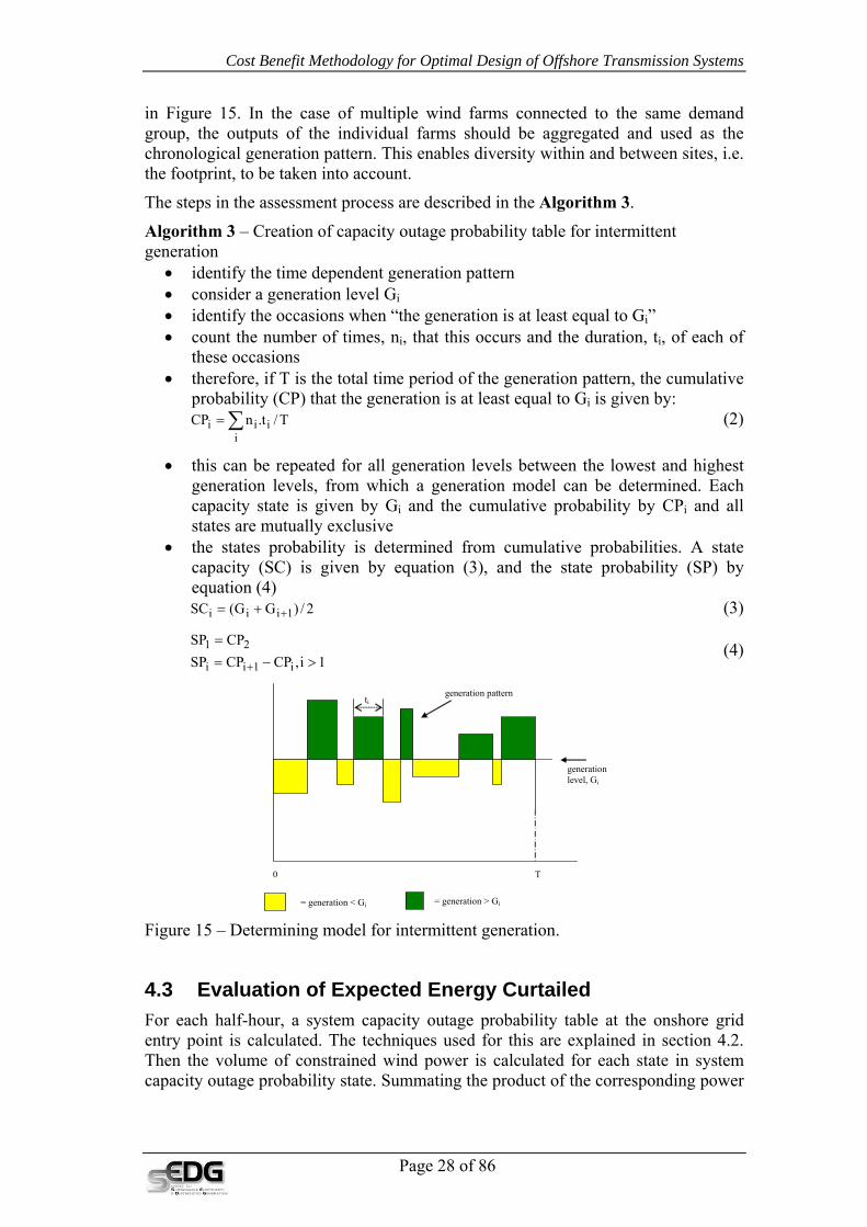
in Figure 15. In the case of multiple wind farms connected to the same demand group, the outputs of the individual farms should be aggregated and used as the chronological generation pattern. This enables diversity within and between sites, i.e. the footprint, to be taken into account.
The steps in the assessment process are described in the Algorithm 3.
Algorithm 3 – Creation of capacity outage probability table for intermittent generation
• identify the time dependent generation pattern • consider a generation level Gi • identify the occasions when “the generation is at least equal to Gi” • count the number of times, ni, that this occurs and the duration, ti, of each of
these occasions • therefore, if T is the total time period of the generation pattern, the cumulative
probability (CP) that the generation is at least equal to Gi is given by: ∑=
iiii T/t.nCP (2)
• this can be repeated for all generation levels between the lowest and highest generation levels, from which a generation model can be determined. Each capacity state is given by Gi and the cumulative probability by CPi and all states are mutually exclusive
• the states probability is determined from cumulative probabilities. A state capacity (SC) is given by equation (3), and the state probability (SP) by equation (4)
2/)GG(SC 1iii ++= (3)
1i,CPCPSPCPSP
i1ii
21>−=
=
+ (4)
ti
T0
generation level, Gi
generation pattern
= generation < Gi = generation > Gi Figure 15 – Determining model for intermittent generation.
4.3 Evaluation of Expected Energy Curtailed For each half-hour, a system capacity outage probability table at the onshore grid entry point is calculated. The techniques used for this are explained in section 4.2. Then the volume of constrained wind power is calculated for each state in system capacity outage probability state. Summating the product of the corresponding power
Page 28 of 86
Page 29 of 86
Cost Benefit Methodology for Optimal Design of Offshore Transmission Systems
that is constrained with and probability of that state, an expected power curtailed is obtained. Summating the product of the expected power curtailed and the duration of each half-hour period, the volume of the expected energy curtailed is evaluated.
4.4 Cost of Expected Energy Curtailed The cost of EEC is given by expression (5), while the calculation of the EEC is explained in section 4.3:
cecEECEECC ⋅= (5)
where:
EECC EEC cost EEC expected energy constrained per year cec capitalised energy cost
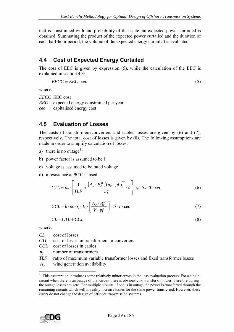
4.5 Evaluation of Losses The costs of transformers/converters and cables losses are given by (6) and (7), respectively. The total cost of losses is given by (8). The following assumptions are made in order to simplify calculation of losses:
a) there is no outage11
b) power factor is assumed to be 1
c) voltage is assumed to be rated voltage
d) a resistance at 90ºC is used
( ) cecTSrS
pfnPATLF
nCTL TTT
TM
WwT ⋅⋅⋅⋅
⎥⎥⎦
⎤
⎢⎢⎣
⎡⋅
⋅⋅+⋅= δ2
2)(1 (6)
cecTpfVPALrnckCCL
MWW
cc ⋅⋅⋅⎟⎟⎠
⎞⎜⎜⎝
⎛⋅⋅
⋅⋅⋅⋅= δ2
(7)
CCLCTLCL += (8)
where:
CL cost of losses CTL cost of losses in transformers or converters CCL cost of losses in cables
Tn number of transformers TLF ratio of maximum variable transformer losses and fixed transformer losses
wA wind generation availability 11 This assumption introduces some relatively minor errors in the loss evaluation process. For a single circuit when there is an outage of that circuit there is obviously no transfer of power, therefore during the outage losses are zero. For multiple circuits, if one is in outage the power is transferred through the remaining circuits which will in reality increase losses for the same power transferred. However, these errors do not change the design of offshore transmission systems.

Page 30 of 86
Cost Benefit Methodology for Optimal Design of Offshore Transmission Systems
MWP output transferred through transformers or
VA/MW rating δ
es loss factor (1 for HVAC, 0.5 for HVDC)
c for cable)
maximum wind generationconverters and cables transformer/converter MTS loss load factor
k current type cablnc number of sets of cables
erature (index T for transformer and r resistance at average tempV cable rating voltage
DC pf = 1) pf power factor (for HVcec capitalised energy cost
rs (T = 8760h) T duration of a year in hou
Page 31 of 86
Cost Benefit Methodology for Optimal Design of Offshore Transmission Systems
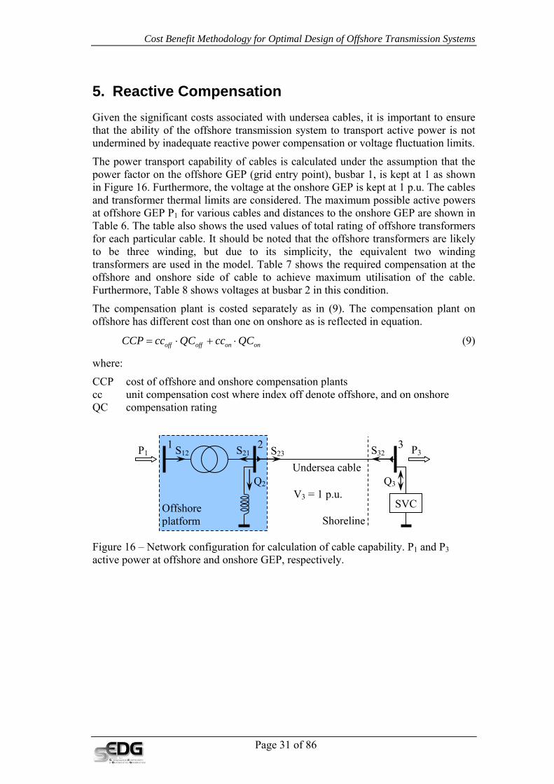
5. Reactive Compensation Given the significant costs associated with undersea cables, it is important to ensure that the ability of the offshore transmission system to transport active power is not undermined by inadequate reactive power compensation or voltage fluctuation limits.
The power transport capability of cables is calculated under the assumption that the power factor on the offshore GEP (grid entry point), busbar 1, is kept at 1 as shown in Figure 16. Furthermore, the voltage at the onshore GEP is kept at 1 p.u. The cables and transformer thermal limits are considered. The maximum possible active powers at offshore GEP P1 for various cables and distances to the onshore GEP are shown in Table 6. The table also shows the used values of total rating of offshore transformers for each particular cable. It should be noted that the offshore transformers are likely to be three winding, but due to its simplicity, the equivalent two winding transformers are used in the model. Table 7 shows the required compensation at the offshore and onshore side of cable to achieve maximum utilisation of the cable. Furthermore, Table 8 shows voltages at busbar 2 in this condition.
The compensation plant is costed separately as in (9). The compensation plant on offshore has different cost than one on onshore as is reflected in equation.
ononoffoff QCccQCccCCP ⋅+⋅= (9)
where:
CCP cost of offshore and onshore compensation plants cc unit compensation cost where index off denote offshore, and on onshore QC compensation rating
P Djapic
V3 = 1 p.u.
1 2 3 P1
SVC
P3 S12 S21 S23 S32
Offshore platform
Q2 Q3
Undersea cable
Shoreline
Figure 16 – Network configuration for calculation of cable capability. P1 and P3 active power at offshore and onshore GEP, respectively.

Cost Benefit Methodology for Optimal Design of Offshore Transmission Systems
Table 6 – Maximum active power output of wind farm in MW Cable parameters Offshore
substation rating (MVA)
Cable length (km) Voltage
(kV) Size
(mm2) Rating (MVA) 25 50 75 100
132
500 169 180 168 168 168 166 630 187 200 186 186 186 184 800 203 220 202 202 202 200.5
1000 217 220 216 216 216 214
220
500 279 280 277.5 277.5 273.5 266 630 308 315 306 306 301.5 293 800 335 360 333.5 333.5 328 319
1000 359 360 357 357 351 341
400
800 603 630 599.5 587 559.5 517 1000 646 630 641.5 628.5 599 553 1200 683 710 679 656 612.5 543 1400 703 710 699 673 625.5 548 1600 718 710 713 684.5 632.5 546 2000 747 800 741.5 711 655 563
Table 7 – Required offshore and onshore compensation in MVAr to maintain the maximum active power transfer capabilities of the offshore transmission system (conditions given in Table 6)
Cable parameters
Offshore compensation (MVAr) Onshore compensation (MVAr)
Cable length (km) Cable length (km) Voltage
(kV) Size
(mm2) 25 50 75 100 25 50 75 100
132
500 0 0 0 12 1.6 21.8 46.8 60 630 0 0 0 13 2.6 22.3 48.8 62.6 800 0 0 0 11 4.4 20.7 47.4 63.6
1000 0 0 0 12 6.3 20.9 50 68
220
500 0 0 22 49 5.4 54 82.2 107.1 630 0 0 26 56 6.8 60.4 89.7 117 800 0 0 30 62 8.7 65.9 95 124.2
1000 0 0 31 66 6.3 68.2 101.4 133.1
400
800 0 67 154 246 68.4 161.6 241.1 322.8 1000 0 66 160 261 67.2 173.7 259.5 346.4 1200 0 107 224 349 105.3 209.7 315.4 423.3 1400 0 115 241 373 111.6 221.7 332.5 449.9 1600 0 125 258 401 119.6 234.1 351.3 472.8 2000 13 143 281 430 123.3 244.7 369.2 497.3
The table above shows that relatively modest amounts of reactive compensation are required to be installed offshore, for cables 132kV and 220kV, while more
Page 32 of 86
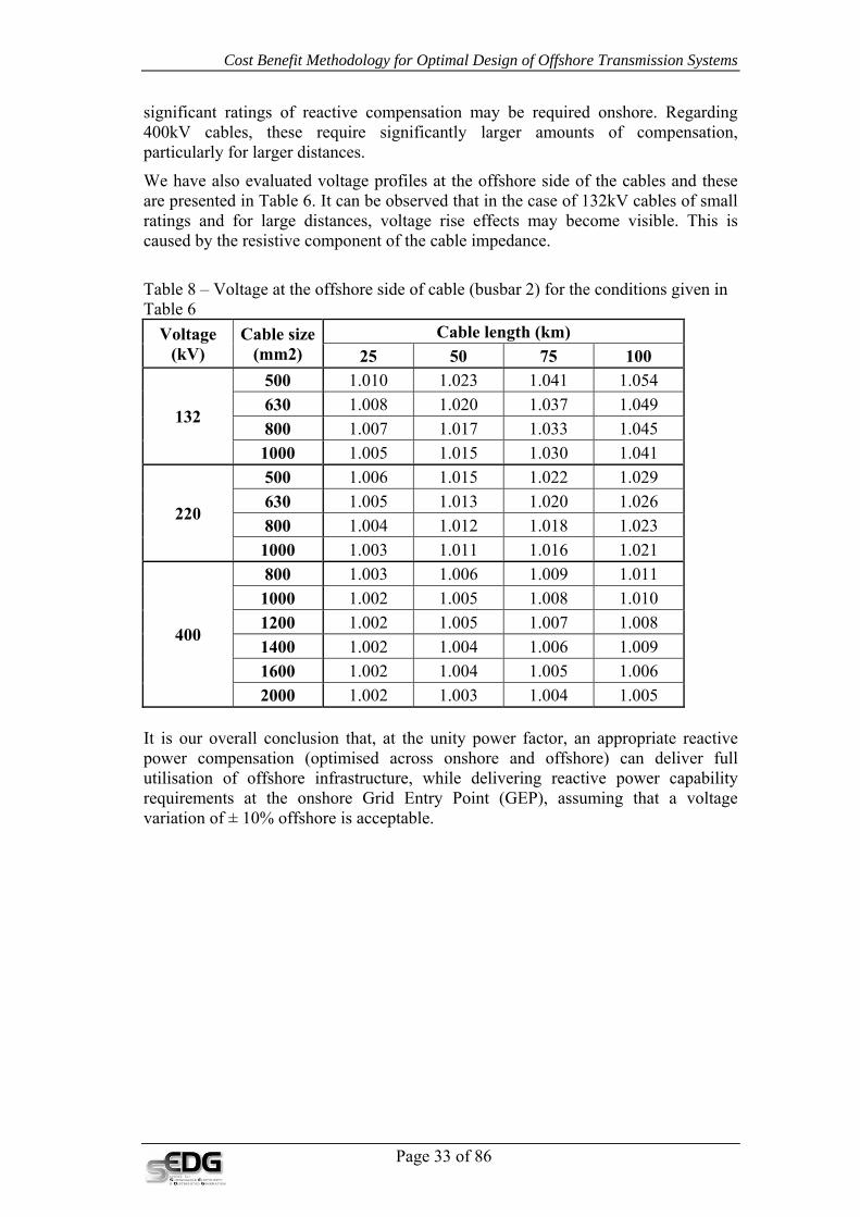
Cost Benefit Methodology for Optimal Design of Offshore Transmission Systems
significant ratings of reactive compensation may be required onshore. Regarding 400kV cables, these require significantly larger amounts of compensation, particularly for larger distances.
We have also evaluated voltage profiles at the offshore side of the cables and these are presented in Table 6. It can be observed that in the case of 132kV cables of small ratings and for large distances, voltage rise effects may become visible. This is caused by the resistive component of the cable impedance.
Table 8 – Voltage at the offshore side of cable (busbar 2) for the conditions given in Table 6
Voltage (kV)
Cable size (mm2)
Cable length (km) 25 50 75 100
132
500 1.010 1.023 1.041 1.054 630 1.008 1.020 1.037 1.049 800 1.007 1.017 1.033 1.045 1000 1.005 1.015 1.030 1.041
220
500 1.006 1.015 1.022 1.029 630 1.005 1.013 1.020 1.026 800 1.004 1.012 1.018 1.023 1000 1.003 1.011 1.016 1.021
400
800 1.003 1.006 1.009 1.011 1000 1.002 1.005 1.008 1.010 1200 1.002 1.005 1.007 1.008 1400 1.002 1.004 1.006 1.009 1600 1.002 1.004 1.005 1.006 2000 1.002 1.003 1.004 1.005
It is our overall conclusion that, at the unity power factor, an appropriate reactive power compensation (optimised across onshore and offshore) can deliver full utilisation of offshore infrastructure, while delivering reactive power capability requirements at the onshore Grid Entry Point (GEP), assuming that a voltage variation of ± 10% offshore is acceptable.
Page 33 of 86

Page 34 of 86
Cost Benefit Methodology for Optimal Design of Offshore Transmission Systems
6. Evaluation of Costs of Assets and Corrective (Post Fault) Maintenance12
The platform and plant costs shown in (10) are generic and consist of (i) fixed costs for foundation, float out and erect and (ii) variable cost for topsides with plant cost being linearly dependent on the number and rating of transformers. The term within the square bracket is the cost multiplier which allows the costs to be adjusted if there are more or less than two transformers at the platform.
[ ] TTTT SncndcFCPPC ⋅⋅⋅−++= 2)2(1 (10)
where:
PPC platform and plant cost FC fixed costs for foundation, float out and erect dc cost factor which allows costing for a different number of
transformers/converters on a platform Tn number of transformers/converters per platform
TS apparent/real power rating of a single transformer/converter
Tc2 cost per MVA/MW quoted for two transformers/converters on a platform The costs of undersea cables shown in (11) are also generic and cover cost of supply and cost of lay and bury and for each specific cable these are given per km. The cost is given for a set of cables which means one for a 3-core cable, three for single-core cables, and two (bipole) single core cables for a DC application.
lcclbccsncCC ⋅+⋅= )( (11)
where:
CC cost of cables nc number of a set of cables ccs cost of supplying of a set of cables cclb cost of lay and bury of a set of cables l length of a cable The cost of corrective maintenance is calculated from reliability parameters and quoted separately.
( ) ( )[ ] CFmcTMTTRFRnmcTMTTRFRnMC ccccTTTT ⋅⋅++⋅+= //1//1 (12)
where:
MC cost of corrective maintenance n number of elements (index T for transformers and c for cables) FR failure rate (1/year) (index T for transformers and c for cables) MTTR mean time to repair (h) (index T for transformers and c for cables) T duration of a year in hours (T = 8760h)
12 In this context, corrective maintenance relates to post-fault replacement or repair of faulty equipment

Cost Benefit Methodology for Optimal Design of Offshore Transmission Systems
mc average cost per maintenance (index T for transformers and c for cables) CF capitalisation factor (years)
Page 35 of 86

Cost Benefit Methodology for Optimal Design of Offshore Transmission Systems
7. Minimum Capacity Factor – X Factor The cost benefit analysis demonstrated that the total optimal capacity of the offshore transmission systems installed can be lower than the maximum export capacity of the wind farm connected due to the cost of installing offshore transmission assets to full capacity (X factor).
Table 9 shows the maximum size of wind farm in MW that will be optimally supplied for different cable configurations. For example, if distance to the shore is 50 km, then a wind farm of a size of between 322 and 352 MW will be optimally connected to the grid with one cable at 220 kV 800 mm2. Dividing cable capabilities given in Table 6 with the corresponding values in Table 9 the X factor is obtained. Table 10 shows these values.
Table 9 – Wind farms capacity (MW) that change cable optimum configuration (change from one cable rating to the next and change in number of cables used).
Wind farms capacity (MW)
Non-diversified wind profile Diversified wind profile
Voltage Number of
cables
Cable size Cable length (km) Cable length (km)
(kV) mm2 25 50 75 100 25 50 75 100
132 1 500 176 178 178 176 188 190 192 194 630 196 196 198 196 208 212 214 214 800 214 216 218 218 230 236 240 240
220 1
500 292 292 290 282 306 310 310 304 630 322 322 320 312 338 342 342 336 800 350 352 346 338 366 372 370 364 1000 392 406 410 408 434 456 470 474
132 2 800 426 428 430 430 450 462 - -
220 2
500 555 565 575 560 600 605 605 595 630 640 645 635 620 665 675 670 660 800 695 700 690 675 720 730 730 715 1000 770 790 795 780 845 875 885 885
3 500 Similar analysis is carried out for the different ratings of transformers. The maximum size of wind farm that can be optimally supplied by two transformers is shown in Table 11. Dividing total transformers rating with the size of corresponding wind farms, the X factors for transformers are obtained. The values are shown in Table 12.
Page 36 of 86

Cost Benefit Methodology for Optimal Design of Offshore Transmission Systems
Table 10 – X factor for cables X factor (%) Non-diversified wind profile Diversified wind profile
Voltage Number of
cables
Cable size Cable length (km) Cable length (km)
(kV) mm2 25 50 75 100 25 50 75 100
132 1 500 95.5 94.4 94.4 94.3 89.4 88.4 87.5 85.6 630 94.9 94.9 93.9 93.9 89.4 87.7 86.9 86.0 800 94.4 93.5 92.7 92.0 87.8 85.6 84.2 83.5
220 1
500 95.0 95.0 94.3 94.3 90.7 89.5 88.2 87.5 630 95.0 95.0 94.2 93.9 90.5 89.5 88.2 87.2 800 95.3 94.7 94.8 94.4 91.1 89.7 88.6 87.6
1000 91.1 87.9 85.6 83.6 82.3 78.3 74.7 71.9 132 2 800 94.8 94.4 94.0 93.3 89.8 87.4 - -
220 2
500 100.0 98.2 95.1 95.0 92.5 91.7 90.4 89.4 630 95.6 94.9 95.0 94.5 92.0 90.7 90.0 88.8 800 96.0 95.3 95.1 94.5 92.6 91.4 89.9 89.2
1000 92.7 90.4 88.3 87.4 84.5 81.6 79.3 77.1 3 500
Table 11 – Wind farm capacity (MW) that change transformer size solution.
Wind farm capacity (MW) Non diversified profile Diversified profile No
transformers Transformers rating (MW)
Length (km) 25 50 75 100 25 50 75 100
2 85 178 178 178 178 188 190 192 192 2 90 188 188 188 188 194 194 194 194 2 95 200 200 200 200 208 212 214 214 2 100 210 210 210 210 216 216 216 222 2 105 220 220 220 220 230 236 240 240 2 140 294 294 294 294 306 310 310 - 2 155 326 326 326 326 338 342 342 336 2 160 336 336 336 338 344 344 344 364 2 165 346 346 346 346 356 356 370 - 2 205 428 428 430 430 450 462 470 474 2 280 585 585 585 585 600 605 605 2 290 610 610 610 610 625 625 625 2 300 630 630 630 630 645 645 645 660 2 310 650 650 650 650 665 675 670 665 2 320 670 670 670 675 685 690 685 715 2 330 690 690 690 690 710 710 730 - 2 360 755 760 760 765 835 835 2 370 775 780 785 780 845 860 2 380 795 795 795 795 - 875 885 885
Page 37 of 86

Cost Benefit Methodology for Optimal Design of Offshore Transmission Systems
Table 12 – X factor for transformers X factor (%) Non diversified profile Diversified profile
No transformers
Transformers rating (MW)
Length (km) 25 50 75 100 25 50 75 100
2 85 95.5 95.5 95.5 95.5 90.4 89.5 88.5 88.5 2 90 95.7 95.7 95.7 95.7 92.8 92.8 92.8 92.8 2 95 95.0 95.0 95.0 95.0 91.3 89.6 88.8 88.8 2 100 95.2 95.2 95.2 95.2 92.6 92.6 92.6 90.1 2 105 95.5 95.5 95.5 95.5 91.3 89.0 87.5 87.5 2 140 95.2 95.2 95.2 95.2 91.5 90.3 90.3 2 155 95.1 95.1 95.1 95.1 91.7 90.6 90.6 92.3 2 160 95.2 95.2 95.2 94.7 93.0 93.0 93.0 87.9 2 165 95.4 95.4 95.4 95.4 92.7 92.7 89.2 2 205 95.8 95.8 95.3 95.3 91.1 88.7 87.2 86.5 2 280 95.7 95.7 95.7 95.7 93.3 92.6 92.6 2 290 95.1 95.1 95.1 95.1 92.8 92.8 92.8 2 300 95.2 95.2 95.2 95.2 93.0 93.0 93.0 90.9 2 310 95.4 95.4 95.4 95.4 93.2 91.9 92.5 93.2 2 320 95.5 95.5 95.5 94.8 93.4 92.8 93.4 89.5 2 330 95.7 95.7 95.7 95.7 93.0 93.0 90.4 2 360 95.4 94.7 94.7 94.1 86.2 86.2 2 370 95.5 94.9 94.3 94.9 87.6 86.0 2 380 95.6 95.6 95.6 95.6 86.9 85.9 85.9
The drivers for minimum capacity factor are:
• Cable length: X reducing with increasing length • Diversity: • Cable size: relatively large value of X • Voltage level: medium value of X • Increase of number of cables: relatively small value of X
Recalculation of X factor for different values of wind farm availabilities is given by the following equation Xa = (A / 0.95) X95 where Xa is X factor for desired availability A and X95 is X factor for 95% availability. The assessment demonstrated that offshore platform capacity should be about 95% of the maximum export capacity of the wind farm connected.
For cable networks, the total optimal capacity installed can be lower than the maximum export capacity of the wind farm connected due to the cost of installing offshore transmission assets to full capacity (X factor in table below). For non-diversified wind profile (appropriate for relatively small wind farms, occupying small geographical areas) the installed network capacity should be above 95% of the maximum output of the wind farm, while in case of diversified wind profile (appropriate for relatively large wind farms occupying relatively large areas) the installed network capacity should be above 90% of the maximum output of the wind
Page 38 of 86

Cost Benefit Methodology for Optimal Design of Offshore Transmission Systems
farm. In cases where this value requires additional cable to be installed, consideration should be given to installation of network capacity below 95% for non-diversified profile and below 90% for diversified profiles. The optimal values of the X factor will be a function of the distance as shown in the table below. For example, consider a wind farm at 100km offshore for which we consider connection of 1 or 2 cables. If the rating of the cable is 77% (or more) of the wind farm installed capacity, installing 2 cables would not be justified.
Table 13 – Minimum capacity factors – X factors (%) for shared connections
X factor (%) Cable length (km)Wind farm profile
Condition - Increase in 25 50 75 100
Non-diversified wind profile
Cable rating >95 Number of cables >91 >88 >86 >84
Diversified wind profile
Cable rating >90 Number of cables >85 >82 >79 >77
Page 39 of 86
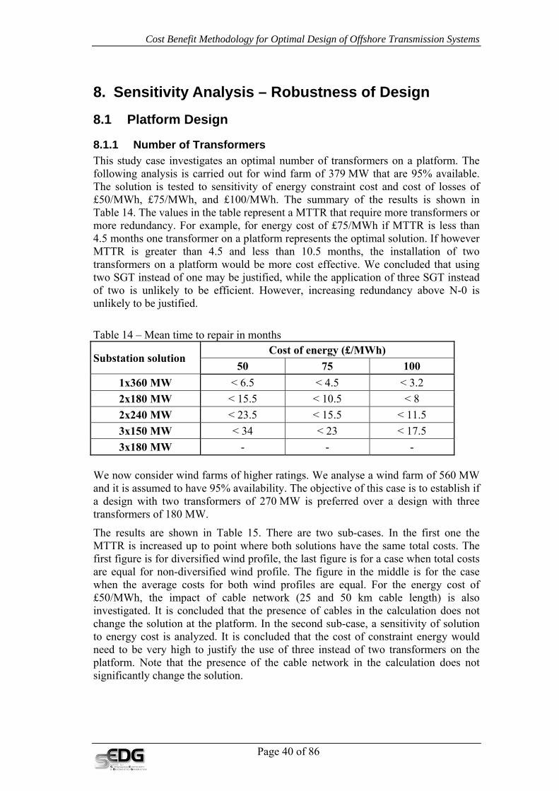
Cost Benefit Methodology for Optimal Design of Offshore Transmission Systems
8. Sensitivity Analysis – Robustness of Design
8.1 Platform Design
8.1.1 Number of Transformers This study case investigates an optimal number of transformers on a platform. The following analysis is carried out for wind farm of 379 MW that are 95% available. The solution is tested to sensitivity of energy constraint cost and cost of losses of £50/MWh, £75/MWh, and £100/MWh. The summary of the results is shown in Table 14. The values in the table represent a MTTR that require more transformers or more redundancy. For example, for energy cost of £75/MWh if MTTR is less than 4.5 months one transformer on a platform represents the optimal solution. If however MTTR is greater than 4.5 and less than 10.5 months, the installation of two transformers on a platform would be more cost effective. We concluded that using two SGT instead of one may be justified, while the application of three SGT instead of two is unlikely to be efficient. However, increasing redundancy above N-0 is unlikely to be justified.
Table 14 – Mean time to repair in months
Substation solution Cost of energy (£/MWh)
50 75 100 1x360 MW < 6.5 < 4.5 < 3.2 2x180 MW < 15.5 < 10.5 < 8 2x240 MW < 23.5 < 15.5 < 11.5 3x150 MW < 34 < 23 < 17.5 3x180 MW - - -
We now consider wind farms of higher ratings. We analyse a wind farm of 560 MW and it is assumed to have 95% availability. The objective of this case is to establish if a design with two transformers of 270 MW is preferred over a design with three transformers of 180 MW.
The results are shown in Table 15. There are two sub-cases. In the first one the MTTR is increased up to point where both solutions have the same total costs. The first figure is for diversified wind profile, the last figure is for a case when total costs are equal for non-diversified wind profile. The figure in the middle is for the case when the average costs for both wind profiles are equal. For the energy cost of £50/MWh, the impact of cable network (25 and 50 km cable length) is also investigated. It is concluded that the presence of cables in the calculation does not change the solution at the platform. In the second sub-case, a sensitivity of solution to energy cost is analyzed. It is concluded that the cost of constraint energy would need to be very high to justify the use of three instead of two transformers on the platform. Note that the presence of the cable network in the calculation does not significantly change the solution.
Page 40 of 86

Cost Benefit Methodology for Optimal Design of Offshore Transmission Systems
Table 15 – Break-even parameters shown in bold. The first figure is associated with diversified wind profile, second represent the average value, while the third refers to non-diversified wind profile
Case Cable length (km) MTTR (months) Energy cost (£/MWh)
MTTR case
- 18 – 21 – 24 50 25 18 – 21 – 24 50 50 18.5 – 21 – 23.5 50 - 12 – 13.5 – 15.5 75 - 9 – 10 – 11.5 100
Energy cost case- 3 300 – 330 – 370
25 3 300 – 330 – 370 50 3 300 – 330 – 360
It can be seen from the two tables above that N-0 is the preferable configuration.
8.1.2 Maximum Rating of a Single Transformer Connection A maximum rating of a single transformer is analysed. As the cost of smaller transformers is not well represented by the generic cost function used, a set of cost data of specific transformers is analysed (in Table 68 of Appendix). The data allows the comparison of platform capacities of 60, 90 and 120 MW. The results are shown in Figure 17, Figure 18 and Figure 19.
Figure 17 shows that the most cost effective solution for a wind capacity of 60 MW carried out through a single platform is a single transformer of 60 MVA. The conclusion is even further reinforced by the fact that two transformers require more expensive busbar and switchgear systems. Similar conclusion can be drawn for a wind capacity of 90 MW, although not as strong as for the previous example. For a wind capacity of 120 MW, it can be seen that solutions with one transformer and two transformers are similar and this is down to the fact that wind power is more or less diversified. Although a full set of data for the assessment of the costs of transformers of higher ratings was not available, the observed trend was considered to be strong enough and a break-even point of 120 MW is proposed.
Page 41 of 86

Cost Benefit Methodology for Optimal Design of Offshore Transmission Systems
0
2
4
6
8
10
12
14
Cos
t (m
£)
Mainenance cost (m£) 3.70 3.70 3.70 3.70 1.85 1.85 3.70 3.70 1.85 1.85 1.85 1.85
Losses cost (m£) 0.68 0.56 0.55 0.47 0.68 0.56 0.52 0.46 0.55 0.47 0.52 0.46
EEC cost (m£) 1.05 0.61 0.26 0.09 2.09 2.07 0.03 0.03 2.09 2.07 2.09 2.07
Platform & plant cost (m£) 7.04 7.04 7.78 7.78 6.56 6.56 8.60 8.60 7.18 7.18 7.85 7.85
1 2 1 2 1 2 1 2 1 2 1 2
2 t. 2 t. 1 t. 2 t. 1 t. 1 t.
30 MW t. 45 MW t. 60 MW t. 90 MW t. 120 MW t.
Test 1 Technology AC Voltage (kV) (All) Wind generation (MW) 60 MW
Transformer rating (MW) Number of transformers Wind profile index
Data
Figure 17 – Platform capacity of 60 MW
0
2
4
6
8
10
12
14
16
Cos
t (m
£)
Mainenance cost (m£) 3.70 3.70 3.70 3.70 1.85 1.85 3.70 3.70 1.85 1.85
Losses cost (m£) 1.01 0.84 0.86 0.73 1.01 0.84 0.77 0.69 0.86 0.73
EEC cost (m£) 1.57 0.91 0.70 0.28 3.14 3.10 0.05 0.05 3.14 3.10
Platform & plant cost (m£) 7.78 7.78 8.60 8.60 7.18 7.18 10.08 10.08 7.85 7.85
1 2 1 2 1 2 1 2 1 2
2 t. 2 t. 1 t. 2 t. 1 t.
45 MW t. 60 MW t. 90 MW t. 120 MW t.
Test 1 Technology AC Voltage (kV) (All) Wind generation (MW) 90 MW
Transformer rating (MW) Number of transformers Wind profile index
Data
Figure 18 – Platform capacity of 90 MW
Page 42 of 86

Page 43 of 86
Cost Benefit Methodology for Optimal Design of Offshore Transmission Systems
Figure 19 – Platform capacity of 120 MW
8.2 Cable System Design
8.2.1 Number of Cables The impact of the design driving parameters MTTR and energy cost is shown on the following two examples.
In the first example, the break-even values of this parameter are calculated such that it makes two different designs, one with a single cable and the other with two cables, equally desirable. To show this, an example constituting of a wind farm rated at 280 MW and availability of 95% is developed. This wind power output can be transported through a single 220 kV 500 mm2 cable. Furthermore, two transformers of 135 MW can supply one or two cables. The transformers’ MTTR are 6 months. The results of the break-even values of the MTTR13 for cables, depending on the cable length and energy costs, are shown in Table 16. Given relatively high values of MTTR, we conclude that a single cable is a preferable solution, as the MTTR would need to be exceptionally high to favour a solution with two cables.
In the second example, a wind farm of 600 MW and availability of 95% is connected through two transformers of 285 MW and two or three 220 kV 630 mm2 cables.
In this example, the break-even values of MTTR are calculated such that two different designs, one with two cables and the other with three cables, are equally efficient. The results are shown in Table 17. Similarly to the previous example, a minimum number of cables is likely to be the optimal value.
13 It should be stressed that MTTR represents an average repair time, so that in some instances actual repairs may last longer than the average value, but there will also be occasions when these will be shorter.
0
2
4
6
8
10
12
14
16
18
Cos
t (m
£)
Mainenance cost (m£) 3.70 3.70 3.70 3.70 1.85 1.85 3.70 3.70
Losses cost (m£) 1.35 1.12 1.10 0.94 1.35 1.12 1.03 0.92
EEC cost (m£) 2.09 1.22 0.52 0.17 4.18 4.14 0.06 0.06
Platform & plant cost (m£) 8.60 8.60 10.08 10.08 7.85 7.85 11.66 11.66
1 2 1 2 1 2 1 22 t. 2 t. 1 t. 2 t.
60 MW t. 90 MW t. 120 MW t.
Test 1 Technology AC Voltage (kV) (All) Wind generation (MW) 120 MW
Transformer rating (MW) Number of transformers Wind profile index
Data

Cost Benefit Methodology for Optimal Design of Offshore Transmission Systems
Table 16 – Break-even parameters shown in bold. The values below break-even favour a single cable while those above favour a two cable design.
Length (km) 25 50 75 100 Fixed value
MTTR case
MTTR (months) Energy cost (£/MWh) 19.5 21 23.5 26.5 50 12.5 13 14 15 75
9 9.5 9.5 10 100
Energy cost case Energy cost (£/MWh) MTTR (months)
300 300 310 310 2 Table 17 – Break-even values of MTTR are shown in bold
Length (km) 25 50 75 100 Fixed value
MTTR case
MTTR (months) Energy cost (£/MWh) 23 24.5 25.5 26 50
14.5 15 15.5 15 75 10 10.5 10.5 10.5 100
Energy cost case Energy cost (£/MWh) MTTR (months)
310 320 310 310 2 From these two examples, it is concluded that design of the cable system should follow the principle of installing a minimum number of cables required to transmit the maximum wind power output.
A sensitivity analysis associated with cable failure rate is also carried out. Three values of failure rate for cables are used in calculation: 0.08 (central value), 0.12 (50% more) and 0.04 (50% less). The other parameters are wind farm availability 95%, MTTR for transformers 6 months, MTTR for cables 2 months. The break-even parameters for a change of number of cables from 1 to 2 or from 2 to 3 for various failure rate are analysed. Table 18 shows these break-even values of MTTR, while Table 19 shows break-even values of energy cost.
Page 44 of 86
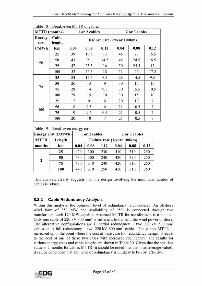
Cost Benefit Methodology for Optimal Design of Offshore Transmission Systems
Table 18 – Break-even MTTR of cables MTTR (months) 1 or 2 cables 2 or 3 cables Energy
cost Cable length Failure rate (1/year.100km)
£/MWh Km 0.04 0.08 0.12 0.04 0.08 0.12
50
25 39 19.5 13 45 23 15.5 50 43 21 14.5 48 24.5 16.5 75 47 23.5 16 50 25.5 17 100 52 26.5 18 51 26 17.5
75
25 24 12.5 8.5 28 14.5 9.5 50 26 13 9 30 15 10 75 28 14 9.5 30 15.5 10.5 100 29 15 10 30 15 10
100
25 17 9 6 20 10 7 50 18 9.5 6 21 10.5 7 75 19 9.5 6.5 21 10.5 7 100 20 10 7 21 10.5 7
Table 19 – Break-even energy costs Energy cost (£/MWh) 1 or 2 cables 2 or 3 cables MTTR Length Failure rate (1/year.100km)months km 0.04 0.08 0.12 0.04 0.08 0.12
2
25 420 300 230 410 310 250 50 430 300 240 420 320 250 75 430 310 240 420 310 250 100 440 310 250 420 310 250
This analysis clearly suggests that the design involving the minimum number of cables is robust.
8.2.2 Cable Redundancy Analysis Within this analysis, the optimum level of redundancy is considered. An offshore wind farm of 350 MW and availability of 95% is connected through two transformers each 170 MW capable. Assumed MTTR for transformers is 6 months. Only one cable of 220 kV 800 mm2 is sufficient to transmit the wind power onshore. The alternative configurations are i) partial redundancy – two 220 kV 500 mm2 cables or ii) full redundancy – two 220 kV 800 mm2 cables. The cables MTTR is increased up to the point where the cost of base case (no redundancy design) is equal to the cost of one of these two cases with increased redundancy. The results for various energy costs and cable lengths are shown in Table 20. Given that the smallest value is 7 months for cables MTTR (it should be noted that this is an average value), it can be concluded that any level of redundancy is unlikely to be cost effective.
Page 45 of 86

Cost Benefit Methodology for Optimal Design of Offshore Transmission Systems
Table 20 – Break-even MTTR (months) shown in bold Cable length Energy cost Redundancy
km £/MWh Reduced Full25 50 15 17.5 75 50 17 20 25 75 9.5 11 75 75 11.5 12.5 25 100 7 8 75 100 7.5 8.5
Table 21 shows break-even MTTR of cables in redundancy study for various energy costs and cable failure rates.
Table 21 – Break-even MTTR of cables MTTR (months) Reduced redundancy Full redundancy Energy
cost Length Failure rate (1/yr.100km)
£/MWh Km 0.04 0.08 0.12 0.04 0.08 0.12
50 25 30 15 10 35 17.5 12 50 34 17 11.5 41 20 14
75 25 19 9.5 6.5 22 11 7.5 50 21 11.5 7 24 12.5 8.5
100 25 14 7 5 16 8 5.5 50 15 7.5 5 17 8.5 6
Again, the analysis clearly suggests that the design involving no redundancy is robust.
8.2.3 Voltage Level This example compares two offshore network configurations with different voltage levels. They supply identical wind farms of 350 MW and availability of 90%. The first configuration consists of two transformers 132/22 kV 160 MW and two three core cables 132 kV 500 mm2. The second configuration consists of one transformer 220/33 kV 320 MW and one three core cable 220 kV 800 mm2. The summary of total costs associated with these configurations for various energy cost is given in Table 22. It can be concluded that one circuit of 220kV is more cost efficient than two circuits of 132kV, independently from their lengths.
Page 46 of 86
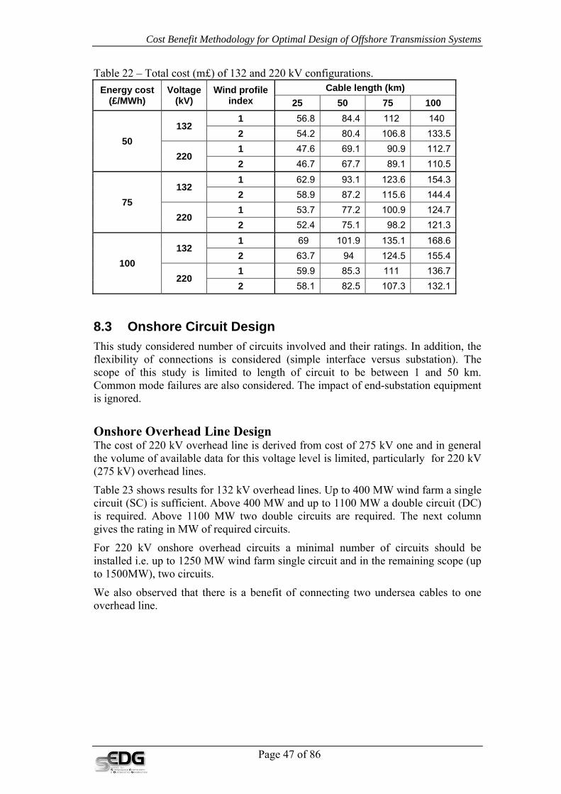
Cost Benefit Methodology for Optimal Design of Offshore Transmission Systems
Table 22 – Total cost (m£) of 132 and 220 kV configurations. Energy cost
(£/MWh) Voltage
(kV) Wind profile
index Cable length (km)
25 50 75 100
50 132
1 56.8 84.4 112 140 2 54.2 80.4 106.8 133.5
220 1 47.6 69.1 90.9 112.7 2 46.7 67.7 89.1 110.5
75 132
1 62.9 93.1 123.6 154.3 2 58.9 87.2 115.6 144.4
220 1 53.7 77.2 100.9 124.7 2 52.4 75.1 98.2 121.3
100 132
1 69 101.9 135.1 168.6 2 63.7 94 124.5 155.4
220 1 59.9 85.3 111 136.7 2 58.1 82.5 107.3 132.1
8.3 Onshore Circuit Design This study considered number of circuits involved and their ratings. In addition, the flexibility of connections is considered (simple interface versus substation). The scope of this study is limited to length of circuit to be between 1 and 50 km. Common mode failures are also considered. The impact of end-substation equipment is ignored.
Onshore Overhead Line Design The cost of 220 kV overhead line is derived from cost of 275 kV one and in general the volume of available data for this voltage level is limited, particularly for 220 kV (275 kV) overhead lines.
Table 23 shows results for 132 kV overhead lines. Up to 400 MW wind farm a single circuit (SC) is sufficient. Above 400 MW and up to 1100 MW a double circuit (DC) is required. Above 1100 MW two double circuits are required. The next column gives the rating in MW of required circuits.
For 220 kV onshore overhead circuits a minimal number of circuits should be installed i.e. up to 1250 MW wind farm single circuit and in the remaining scope (up to 1500MW), two circuits.
We also observed that there is a benefit of connecting two undersea cables to one overhead line.
Page 47 of 86
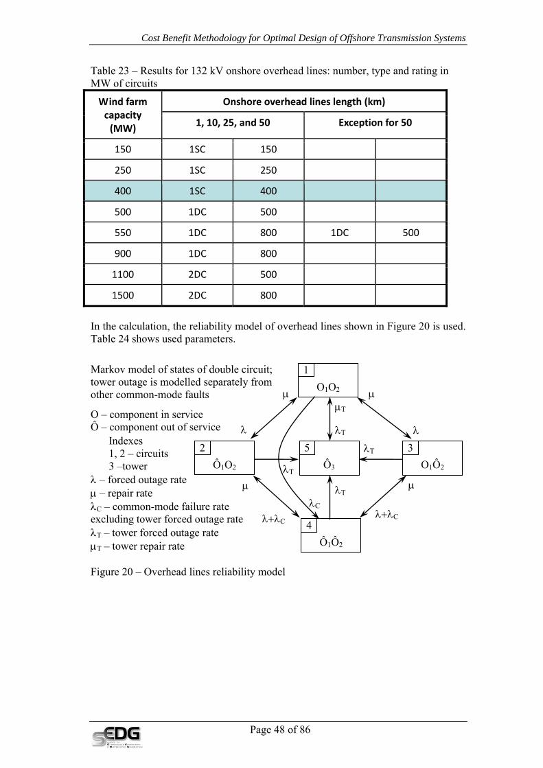
Cost Benefit Methodology for Optimal Design of Offshore Transmission Systems
Table 23 – Results for 132 kV onshore overhead lines: number, type and rating in MW of circuits
Wind farm capacity (MW)
Onshore overhead lines length (km)
1, 10, 25, and 50 Exception for 50
150 1SC 150
250 1SC 250
400 1SC 400
500 1DC 500
550 1DC 800 1DC 500
900 1DC 800
1100 2DC 500
1500 2DC 800
In the calculation, the reliability model of overhead lines shown in Figure 20 is used. Table 24 shows used parameters.
λ – forced outage rate μ – repair rate λC – common-mode failure rate excluding tower forced outage rateλT – tower forced outage rate μT – tower repair rate
1O1O2
4Ô1Ô2
3 O1Ô2
λC
λ+λC
λ
μ μ
μ
O – component in service Ô – component out of service
Markov model of states of double circuit; tower outage is modelled separately from other common-mode faults
λ+λC
5Ô3
λT
λT
λT
λT
μT
λ
2 Ô1O2
μ
Indexes 1, 2 – circuits 3 –tower
Figure 20 – Overhead lines reliability model
Page 48 of 86

Cost Benefit Methodology for Optimal Design of Offshore Transmission Systems
Table 24 – Parameters for Markov model of overhead lines Volta
ge (kV)
FOR
(1/y.100km)
MTTR (h)
CMFOR (1/y.100km)
TFOR (1/y.100km)
TMTTR (h) OC TOC
(£k)
132 SC 0.11 26.2 0 0 - £56.4k -
DC 0.1 21.6 0 0.01 72 £22.0k 400
220 SC 0.69799 56 0 0 - 1.5% -
DC 0.6714 56 0.02659 0 - 1.5% -
where FOR forced outage rate MTTR 1/repair rate CMFOR common-mode failure rate TFOR tower forced outage rate TMTTR 1/tower repair rate OC outage cost TOC tower outage cost
8.4 Onshore Substation Design Design of onshore substation is conceptually similar to those offshore, described above. The outputs of exercise are the optimal number and ratings of transformers. Data set however included typical ratings (note that costs of 300MVA (400 or 275/132 kV) is similar to costs of 1100MVA (400/220 kV) transformers).
It is recommended that number of transformer in 400/220 kV substation should be one for up to 640MW of wind power and double above 640 MW. Three transformers are not justified within the scope of wind farm up to 1500 MW.
For onshore transformation to 132 kV it is recommended a minimum number of transformers of 240 MVA in onshore substation without redundancy as shown in Table 25.
Table 25 – Wind farm ratings for which a breakeven costs are obtained (for wind farm ratings above 500 MW only diversified wind profile, wind profile index 2, are used)
Voltages (kV)
Number Transformers rating (MVA)
240 300 360 400 460
400/132 1 vs. 2 260 320 380 420 480
2 vs. 3 500 660 780 860 980
275/132 1 vs. 2 260 320 380 400 440
2 vs. 3 500 660 780 840 940
Page 49 of 86
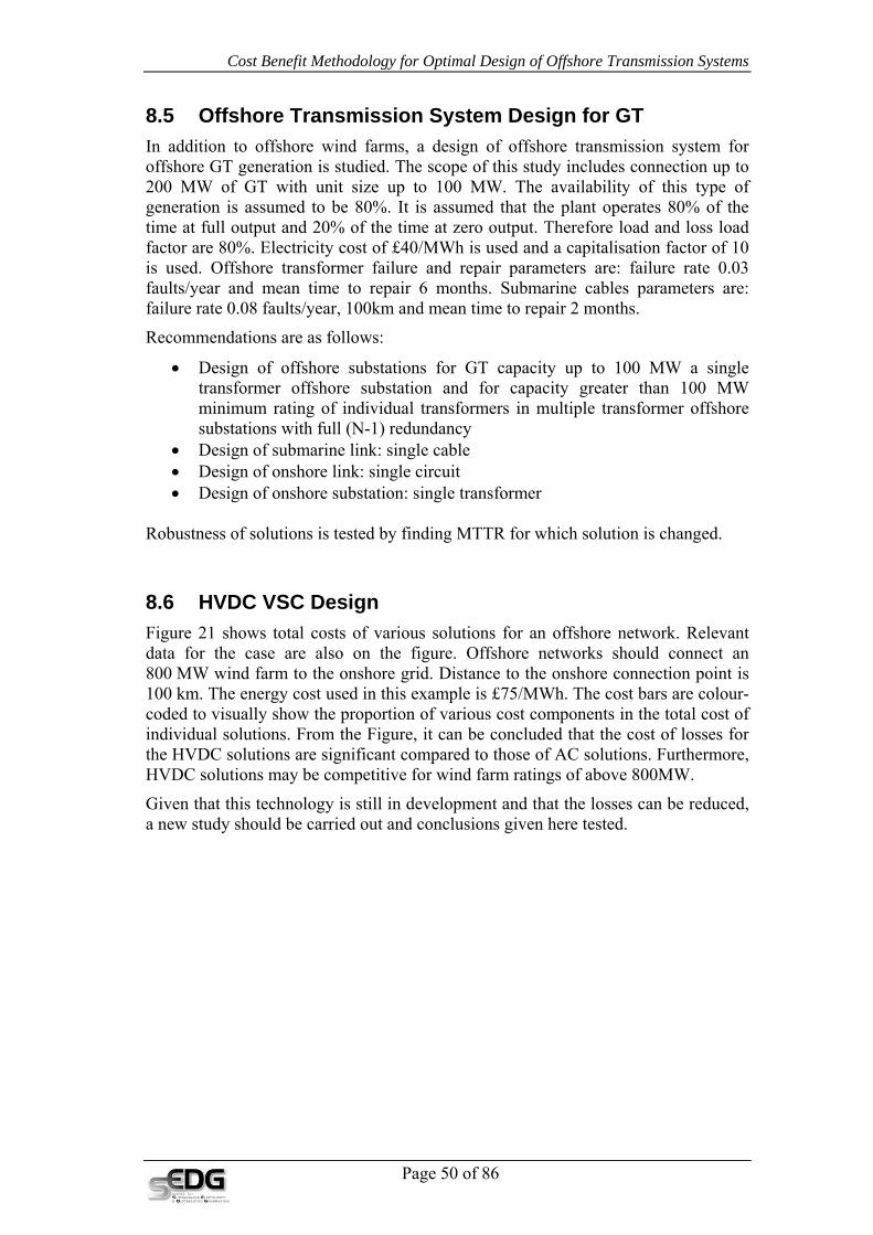
Cost Benefit Methodology for Optimal Design of Offshore Transmission Systems
8.5 Offshore Transmission System Design for GT In addition to offshore wind farms, a design of offshore transmission system for offshore GT generation is studied. The scope of this study includes connection up to 200 MW of GT with unit size up to 100 MW. The availability of this type of generation is assumed to be 80%. It is assumed that the plant operates 80% of the time at full output and 20% of the time at zero output. Therefore load and loss load factor are 80%. Electricity cost of £40/MWh is used and a capitalisation factor of 10 is used. Offshore transformer failure and repair parameters are: failure rate 0.03 faults/year and mean time to repair 6 months. Submarine cables parameters are: failure rate 0.08 faults/year, 100km and mean time to repair 2 months.
Recommendations are as follows:
• Design of offshore substations for GT capacity up to 100 MW a single transformer offshore substation and for capacity greater than 100 MW minimum rating of individual transformers in multiple transformer offshore substations with full (N-1) redundancy
• Design of submarine link: single cable • Design of onshore link: single circuit • Design of onshore substation: single transformer
Robustness of solutions is tested by finding MTTR for which solution is changed.
8.6 HVDC VSC Design Figure 21 shows total costs of various solutions for an offshore network. Relevant data for the case are also on the figure. Offshore networks should connect an 800 MW wind farm to the onshore grid. Distance to the onshore connection point is 100 km. The energy cost used in this example is £75/MWh. The cost bars are colour-coded to visually show the proportion of various cost components in the total cost of individual solutions. From the Figure, it can be concluded that the cost of losses for the HVDC solutions are significant compared to those of AC solutions. Furthermore, HVDC solutions may be competitive for wind farm ratings of above 800MW.
Given that this technology is still in development and that the losses can be reduced, a new study should be carried out and conclusions given here tested.
Page 50 of 86
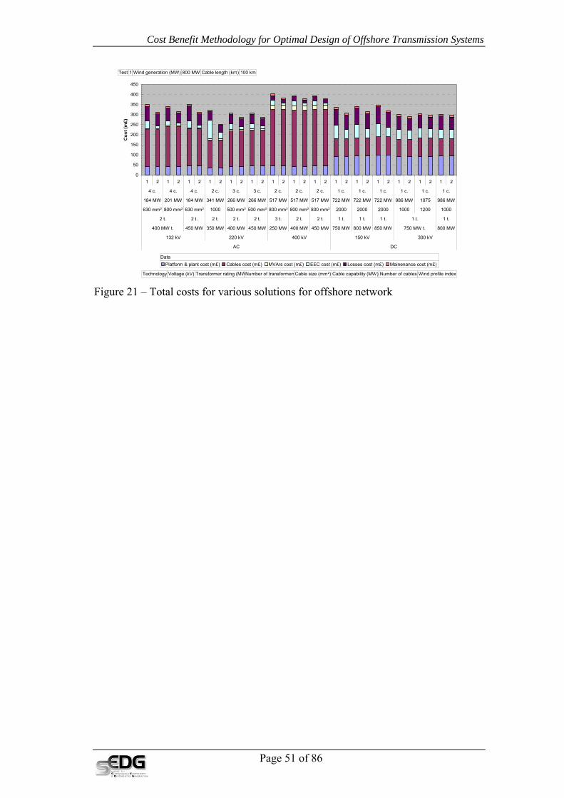
Cost Benefit Methodology for Optimal Design of Offshore Transmission Systems
0
50
100
150
200
250
300
350
400
450
1 2 1 2 1 2 1 2 1 2 1 2 1 2 1 2 1 2 1 2 1 2 1 2 1 2 1 2 1 2
4 c. 4 c. 4 c. 2 c. 3 c. 3 c. 2 c. 2 c. 2 c. 1 c. 1 c. 1 c. 1 c. 1 c. 1 c.
184 MW 201 MW 184 MW 341 MW 266 MW 266 MW 517 MW 517 MW 517 MW 722 MW 722 MW 722 MW 986 MW 1075 986 MW
630 mm² 800 mm² 630 mm² 1000 500 mm² 500 mm² 800 mm² 800 mm² 800 mm² 2000 2000 2000 1000 1200 1000
2 t. 2 t. 2 t. 2 t. 2 t. 3 t. 2 t. 2 t. 1 t. 1 t. 1 t. 1 t. 1 t.
400 MW t. 450 MW 350 MW 400 MW 450 MW 250 MW 400 MW 450 MW 750 MW 800 MW 850 MW 750 MW t. 800 MW
132 kV 220 kV 400 kV 150 kV 300 kV
AC DC
Cos
t (m
£)
Platform & plant cost (m£) Cables cost (m£) MVArs cost (m£) EEC cost (m£) Losses cost (m£) Mainenance cost (m£)
Test 1 Wind generation (MW) 800 MW Cable length (km) 100 km
Technology Voltage (kV) Transformer rating (MWNumber of transformersCable size (mm²) Cable capability (MW) Number of cables Wind profile index
Data
Figure 21 – Total costs for various solutions for offshore network
Page 51 of 86

Cost Benefit Methodology for Optimal Design of Offshore Transmission Systems
9. Impact of Planned Outages of Offshore Infrastructure for Wind Based Generation
9.1 Background From the information and advice on maintenance practices from three DNOs covering 132/33kV transformers and 132 kV lines, the following generic preventive maintenance schedule is derived. For 132/33kV transformers the minor maintenance occurs every 4 years with duration of 2 to 5 days while major occurs every 8 years with duration of 6 to 10 days. The maintenance of overhead lines 132 kV every 15 years and it is coordinated with transformer maintenance.
Information on maintenance practices for 400/132kV transformers and 275/400kV OH lines was received from National Grid.
The following questions are considered
• Maximum ratings for single on & offshore transformers & circuits • Minimum rating of on and offshore multi-transformer substations and circuit
9.2 Methodology for Inclusion of Impact of Planned Outages on Design of Offshore Transmission Equipment
The step 2 is added to the previous methodology which is now as follows
• Step 1: Carry out an initial design that is based on the solutions that do not include preventive maintenance outages
• Step 2: Increase the ratings of transformers to balance the additional capital cost and expecting energy curtailed due to preventive maintenance outage
It is assumed that the preventive maintenance period will be conducted over three summer months, i.e. Jun to August. For that purpose a load duration curve covering that period is shown in Figure 22 and curtailed energy factor in Figure 23. It can be seen that during that period load factor of wind farm is 24% which is less than overall annual load factor of 40%. Furthermore, peak output of wind generation during this period is about 83% of available capacity.
Page 52 of 86
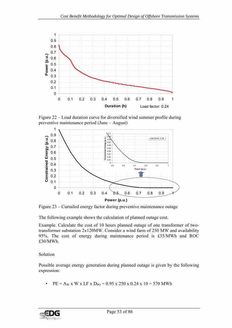
Cost Benefit Methodology for Optimal Design of Offshore Transmission Systems
00.10.20.30.40.50.60.70.80.9
1
0 0.1 0.2 0.3 0.4 0.5 0.6 0.7 0.8 0.9 1
Duration (h)
Pow
er (p
.u.)
Load factor: 0.24
Figure 22 – Load duration curve for diversified wind summer profile during preventive maintenance period (June – August)
00.10.20.30.40.50.60.70.80.9
1
0 0.1 0.2 0.3 0.4 0.5 0.6 0.7 0.8 0.9 1
Power (p.u.)
Cons
train
ed E
nerg
y (p
.u.) Load factor: 0.24
00.010.020.030.040.050.060.070.080.090.1
0.5 0.6 0.7 0.8 0.9 1
Power (p.u.)
Cons
trai
ned
Ener
gy (p
.u.) Load factor: 0.24
Figure 23 – Curtailed energy factor during preventive maintenance outage The following example shows the calculation of planned outage cost.
Example. Calculate the cost of 10 hours planned outage of one transformer of two-transformer substation 2x120MW. Consider a wind farm of 250 MW and availability 95%. The cost of energy during maintenance period is £35/MWh and ROC £30/MWh.
Solution Possible average energy generation during planned outage is given by the following expression:
• PE = AW x W x LF x DPO = 0.95 x 250 x 0.24 x 10 = 570 MWh
Page 53 of 86

Cost Benefit Methodology for Optimal Design of Offshore Transmission Systems
where PE – possible energy (MWh), AW – wind farm availability, W – wind farm rating (MW), LF – load factor during maintenance, DPO – duration of planned outage (h)
Planned outage EEC is given as
• POEEC = N x PE x CEF = 2 x 570 x 0.08 = 91 MWh
where POEEC – planned outage EEC (MWh), N – number of planned outages per year (2), CEF – curtailed energy factor obtained from Figure 23 (X axis – 120/250 = 0.48 and Y axis then 0.8)
Finally, cost of planned outage EEC is
• CPOEEC = POEEC x CE x CF = 91 x 65 x 10 = £59,150 ≅ £0.059m
where CPOEEC – cost of POEEC (£), CE – cost of energy (£/MWh), CF – capitalisation factor
9.3 Design of Offshore and Onshore Substation
9.3.1 Two Transformers per Offshore and Onshore Substation Designs of both onshore and offshore substations are considered simultaneously. Both substations have two transformers. It is assumed that, during preventive maintenance period, one transformer is in service while the other is on planned outage. Planned outages of both on and offshore substations are of the same durations. The average maintenance duration is between 25 and 55 hours. Two wind farm ratings are considered: (i) 250 MW and (ii) 480 MW and results shown in Table 26 and Table 27, respectively. Availability of wind farms is 95%.
Table 26 – Additional cost due to maintenance for case of wind farm of 250 MW Offshore platform (MVA) 2x120 2x180 2x240
Onshore substation (MVA) 2x120 2x180 2x240
Additional investment (£m) 0 6.60 13.20
Forced outage EEC (£m capitalised) 3.92 0.83 0.13
Additional cost to base case (£m) Base case 3.51 9.41
Planned outage EEC cost (£m, capitalised over 25 years)
20 hours (2x1 day) 0.056 0.001 0
116 hours (2x3 days) 0.324 0.007 0
212 hours (2x5 days) 0.593 0.013 0
308 hours (2x7 days) 0.862 0.018 0
Page 54 of 86

Cost Benefit Methodology for Optimal Design of Offshore Transmission Systems
Table 27 – Additional cost due to maintenance for case of wind farm of 480 MW Offshore platform (MVA) 2x230 2x345 2x460
Onshore substation (MVA) 2x230 2x345 2x460
Additional investment (£m) 0 12.65 25.30
Forced outage EEC (£m capitalised) 7.53 1.60 0.26
Additional cost to base case (£m) Base case 6.71 21.63
Planned outage EEC cost (£m, capitalised over 25 years)
20 hours (2x1 day) 0.107 0.002 0
116 hours (2x3 days) 0.623 0.013 0
212 hours (2x5 days) 1.139 0.024 0
308 hours (2x7 days) 1.654 0.035 0
For example of wind farm of 480 MW shown in Table 27, even if duration of planned outage is 2 weeks, the benefit will be £1.6m (1.654-0.035) which is far below additional cost of £6.71m to achieve that benefit. It can be concluded that for solutions with onshore and offshore substations with 2 transformers, there is no impact of planned outages on the design.
9.3.2 Single Transformer per Offshore Platform In this section, the maximum rating for single-transformer platform is examined. Given a single-transformer platform and small rating, this study can be performed only on platform and not considering submarine cables, onshore circuits and onshore substation. It is looking for a case when the additional cost of installing two transformers is smaller than the benefit it brings. Three sizes of wind farm (i) 60 MW, (ii) 90 MW and (iii) 120 MW are considered and results are shown in Table 28, Table 29 and Table 30, respectively. These sizes coincide with the typical transformer ratings. The wind farm availability is 95% and two durations of planned outage are considered 10 and 58 hours per transformer.
Page 55 of 86

Cost Benefit Methodology for Optimal Design of Offshore Transmission Systems
Table 28 – Additional cost and benefit of installing two transformers for wind farm of 60 MW Offshore platform (MVA) 1x60 2x30 2x45
Additional investment (£m) 0 0.94 1.79
Corrective maintenance/repair cost (£m) 0.74 1.48 1.48
EEC cost (£m, capitalised over 25 years)
Forced outage 2.07 0.70 0.13
Planned outage 10 h 0.09 0.01 0.00
Planned outage 58 h 0.52 0.08 0.00
Total PO 10 h / PO 58 h (£m) 2.9/3.32 2.2/2.26 1.61/1.61
Benefit (£m) 0/0 0.7/1.06 1.29/1.71
Table 29 – Additional cost and benefit of installing two transformers for wind farm of 90 MW Offshore platform (MVA) 1x90 2x45 2x60
Additional investment (£m) 0 1.05 2.02
Corrective maintenance/repair cost (£m) 0.74 1.48 1.48
EEC cost (£m, capitalised over 25 years)
Forced outage 3.10 1.05 0.38
Planned outage 10 h 0.13 0.02 0.00
Planned outage 58 h 0.77 0.12 0.01
Total PO 10 h / PO 58 h (£m) 3.97/4.61 2.55/2.65 1.86/1.86
Benefit (£m) 0/0 1.42/1.96 2.12/2.75
Table 30 – Additional cost and benefit of installing two transformers for wind farm of 120 MW Offshore platform (MVA) 1x120 2x60 2x90
Additional investment (£m) 0 1.24 2.98
Corrective maintenance/repair cost (£m) 0.74 1.48 1.48
EEC cost (£m, capitalised over 25 years)
Forced outage 4.13 1.40 0.26
Planned outage 10 h 0.18 0.03 0.00
Planned outage 58 h 1.03 0.16 0.00
Total PO 10 h / PO 58 h (£m) 5.05/5.73 2.91/3.01 1.74/1.74
Benefit (£m) 0/0 2.14/2.71 3.31/3.99
Page 56 of 86

Cost Benefit Methodology for Optimal Design of Offshore Transmission Systems
For wind farm of 60 MW the benefit of having two transformer of 30 MW and considering that duration of planned outage is 10 hours on average is £0.7m while additional cost would be £0.94m (see Table 28). Similarly for wind farm of 90 MW the benefit of having 2 transformers of 45 MVA instead of one of 90 MVA is £1.42m outweigh the additional investment cost of £1.05m (see Table 29). Recommendation is that the maximum rating of a single-transformer platform is 90MW. This finding would be strengthened when considering overlaps with onshore assets maintenance.
9.3.3 Single Transformer per Onshore Substation In order to find out the maximum size of a single-transformer substation the several cases are considered. The study is performed for the following rating of wind farms 125 MW, 180 MW, 250 MW and 310 MW and results are shown in Table 31, Table 32, Table 33 and Table 34, respectively. The results are presented for the following generic planned outage durations: 10, 58, 106 and 154 hours per transformer.
Table 31 – Additional cost and benefit of installing two transformers at onshore substation. Offshore substation consists of 2 transformers of 60 MW each. Onshore substation 1x120 MVA 2x120 MVA
Additional investment (£m) 0 3.94
Onshore transformers corrective maintenance cost (£m) 0.25 0.50
EEC cost (£m, capitalised over 25 years)
Forced outage 0.95 0.00
Planned outage 10/58/106/154 h 0.19/1.07/1.96/2.85 0.00
Total (£m) 1.47/2.75/4.03/5.31 0.5/0.5/0.5/0.5
Benefit (£m) 0 0.97/2.25/3.53/4.81
Table 32 – Additional cost and benefit of installing two transformers at onshore substation. Offshore substation consists of 2 transformers of 90 MW each. Onshore substation 1x180 MVA 2x120 MVA
Additional investment (£m) 0 3.76
Onshore transformers corrective maintenance cost (£m) 0.25 0.50
EEC cost (£m, capitalised over 25 years)
Forced outage 1.37 0.15
Planned outage 10/58/106/154 h 0.27/1.55/2.83/4.11 0.00
Total (£m) 1.89/3.17/4.45/5.73 0.65/0.65/0.65/0.65
Benefit (£m) 0 1.24/2.52/3.8/5.08
Page 57 of 86
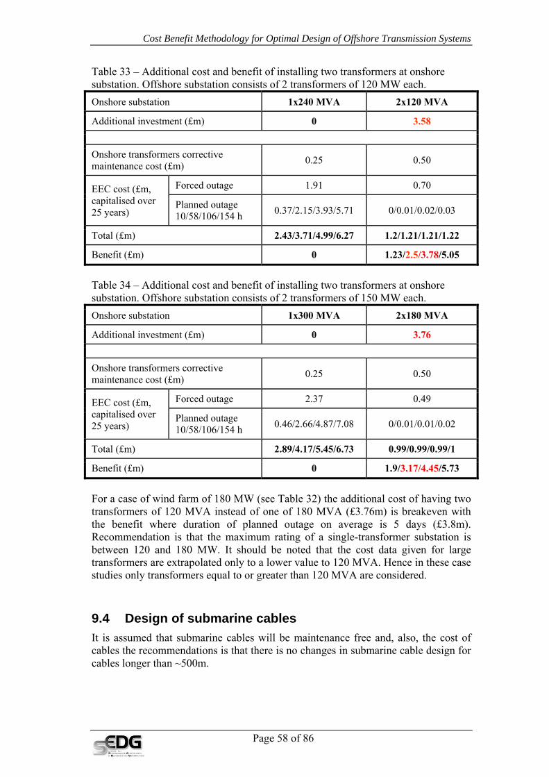
Cost Benefit Methodology for Optimal Design of Offshore Transmission Systems
Table 33 – Additional cost and benefit of installing two transformers at onshore substation. Offshore substation consists of 2 transformers of 120 MW each. Onshore substation 1x240 MVA 2x120 MVA
Additional investment (£m) 0 3.58
Onshore transformers corrective maintenance cost (£m) 0.25 0.50
EEC cost (£m, capitalised over 25 years)
Forced outage 1.91 0.70
Planned outage 10/58/106/154 h 0.37/2.15/3.93/5.71 0/0.01/0.02/0.03
Total (£m) 2.43/3.71/4.99/6.27 1.2/1.21/1.21/1.22
Benefit (£m) 0 1.23/2.5/3.78/5.05
Table 34 – Additional cost and benefit of installing two transformers at onshore substation. Offshore substation consists of 2 transformers of 150 MW each. Onshore substation 1x300 MVA 2x180 MVA
Additional investment (£m) 0 3.76
Onshore transformers corrective maintenance cost (£m) 0.25 0.50
EEC cost (£m, capitalised over 25 years)
Forced outage 2.37 0.49
Planned outage 10/58/106/154 h 0.46/2.66/4.87/7.08 0/0.01/0.01/0.02
Total (£m) 2.89/4.17/5.45/6.73 0.99/0.99/0.99/1
Benefit (£m) 0 1.9/3.17/4.45/5.73
For a case of wind farm of 180 MW (see Table 32) the additional cost of having two transformers of 120 MVA instead of one of 180 MVA (£3.76m) is breakeven with the benefit where duration of planned outage on average is 5 days (£3.8m). Recommendation is that the maximum rating of a single-transformer substation is between 120 and 180 MW. It should be noted that the cost data given for large transformers are extrapolated only to a lower value to 120 MVA. Hence in these case studies only transformers equal to or greater than 120 MVA are considered.
9.4 Design of submarine cables It is assumed that submarine cables will be maintenance free and, also, the cost of cables the recommendations is that there is no changes in submarine cable design for cables longer than ~500m.
Page 58 of 86

Cost Benefit Methodology for Optimal Design of Offshore Transmission Systems
9.5 Design of Onshore Circuit
9.5.1 Design of Overhead Line 132 kV The results of the analysis are shown in Table 35. It can be seen that for wind farm of 150 MW a single onshore circuit is sufficient. For wind farm of 250 MW for short distances double circuit is optimal while for the long distances single circuit is optimal. For wind farm of 400 MW the optimal solution is double circuit. Details of this analysis are shown from Table 36 to Table 47. The onshore substation is not considered and calculation is carried out for two planned outage durations 10 and 58 hours per overhead circuit.
Table 35 – Results for 132kV onshore overhead lines (with generic maintenance of OH lines)
Length (km) Wind farm capacity (MW)
150 250 400
1 SC DC DC
10 SC SC/DC DC
25 SC SC DC
50 SC SC SC/DC
• SC – Single circuit • DC – Double circuit
Table 36 – Additional cost and benefit of different onshore overhead circuit of length of 1km. Rating of wind farm is 150 MW, availability 95%. Offshore substation consists of 2 transformers of 75 MW each. Submarine cable 132 kV 1x500 mm2 50 km is maintenance free. Onshore circuit 1SC=150MVA 1DC=300MVA 2SC=300MVA
Additional investment (£m) 0 0.25 0.45
Cost of onshore circuits losses (£m) 0.01 0.00 0.00
Onshore circuits maintenance cost (£m) 0.00 0.00 0.00
EEC cost (£m, capitalised over 25 years)
Forced outage 0.00 0.00 0.00
Planned outage 10 h 0.22 0.00 0.00
Planned outage 58 h 1.29 0.00 0.00
Total PO 10 h / PO 58 h (£m) 0.23/1.3 0.01/0.01 0.01/0.01
Benefit (£m) 0/0 0.23/1.29 0.23/1.29
Page 59 of 86

Cost Benefit Methodology for Optimal Design of Offshore Transmission Systems
Table 37 – Additional cost and benefit of different onshore overhead circuit of length of 10km. Rating of wind farm is 150 MW, availability 95%. Offshore substation consists of 2 transformers of 75 MW each. Submarine cable 132 kV 1x500 mm2 50 km is maintenance free. Onshore circuit 1SC=150MVA 1DC=300MVA 2SC=300MVA
Additional investment (£m) 0 2.50 4.50
Cost of onshore circuits losses (£m) 0.08 0.04 0.04
Onshore circuits maintenance cost (£m) 0.01 0.01 0.01
EEC cost (£m, capitalised over 25 years)
Forced outage 0.01 0.00 0.00
Planned outage 10 h 0.22 0.00 0.00
Planned outage 58 h 1.29 0.00 0.00
Total PO 10 h / PO 58 h (£m) 0.32/1.39 0.05/0.05 0.05/0.05
Benefit (£m) 0/0 0.27/1.34 0.27/1.34
Table 38 – Additional cost and benefit of different onshore overhead circuit of length of 25km. Rating of wind farm is 150 MW, availability 95%. Offshore substation consists of 2 transformers of 75 MW each. Submarine cable 132 kV 1x500 mm2 50 km is maintenance free. Onshore circuit 1SC=150MVA 1DC=300MVA 2SC=300MVA
Additional investment (£m) 0.00 6.25 11.25
Cost of onshore circuits losses (£m) 0.21 0.10 0.10
Onshore circuits maintenance cost (£m) 0.02 0.02 0.03
EEC cost (£m, capitalised over 25 years)
Forced outage 0.03 0.01 0.00
Planned outage 10 h 0.22 0.00 0.00
Planned outage 58 h 1.29 0.00 0.00
Total PO 10 h / PO 58 h (£m) 0.47/1.54 0.13/0.13 0.13/0.13
Benefit (£m) 0/0 0.34/1.41 0.34/1.41
Page 60 of 86

Cost Benefit Methodology for Optimal Design of Offshore Transmission Systems
Table 39 – Additional cost and benefit of different onshore overhead circuit of length of 50km. Rating of wind farm is 150 MW, availability 95%. Offshore substation consists of 2 transformers of 75 MW each. Submarine cable 132 kV 1x500 mm2 50 km is maintenance free. Onshore circuit 1SC=150MVA 1DC=300MVA 2SC=300MVA
Additional investment (£m) 0.00 12.50 22.50
Cost of onshore circuits losses (£m) 0.42 0.21 0.21
Onshore circuits maintenance cost (£m) 0.03 0.04 0.06
EEC cost (£m, capitalised over 25 years)
Forced outage 0.06 0.01 0.00
Planned outage 10 h 0.22 0.00 0.00
Planned outage 58 h 1.29 0.00 0.00
Total PO 10 h / PO 58 h (£m) 0.73/1.79 0.26/0.26 0.27/0.27
Benefit (£m) 0/0 0.46/1.53 0.46/1.52
Table 40 – Additional cost and benefit of different onshore overhead circuit of length of 1km. Rating of wind farm is 250 MW, availability 95%. Offshore substation consists of 2 transformers of 120 MW each. Submarine cable 132 kV 2x500 mm2 50 km is maintenance free. Onshore circuit 1SC=250MVA 1DC=300MVA 2SC=250MVA
Additional investment (£m) 0.00 0.10 0.60
Cost of onshore circuits losses (£m) 0.02 0.01 0.01
Onshore circuits maintenance cost (£m) 0.00 0.00 0.00
EEC cost (£m, capitalised over 25 years)
Forced outage 0.00 0.00 0.00
Planned outage 10 h 0.37 0.00 0.00
Planned outage 58 h 2.15 0.00 0.00
Total PO 10 h / PO 58 h (£m) 0.4/2.17 0.01/0.01 0.01/0.01
Benefit (£m) 0/0 0.38/2.16 0.38/2.16
Page 61 of 86

Cost Benefit Methodology for Optimal Design of Offshore Transmission Systems
Table 41 – Additional cost and benefit of different onshore overhead circuit of length of 10km. Rating of wind farm is 250 MW, availability 95%. Offshore substation consists of 2 transformers of 120 MW each. Submarine cable 132 kV 2x500 mm2 50 km is maintenance free. Onshore circuit 1SC=250MVA 1DC=300MVA 2SC=250MVA
Additional investment (£m) 0.00 1.00 6.00
Cost of onshore circuits losses (£m) 0.23 0.12 0.12
Onshore circuits maintenance cost (£m) 0.01 0.01 0.01
EEC cost (£m, capitalised over 25 years)
Forced outage 0.02 0.01 0.00
Planned outage 10 h 0.37 0.00 0.00
Planned outage 58 h 2.15 0.00 0.00
Total PO 10 h / PO 58 h (£m) 0.63/2.4 0.13/0.13 0.13/0.13
Benefit (£m) 0/0 0.5/2.27 0.5/2.28
Table 42 – Additional cost and benefit of different onshore overhead circuit of length of 25km. Rating of wind farm is 250 MW, availability 95%. Offshore substation consists of 2 transformers of 120 MW each. Submarine cable 132 kV 2x500 mm2 50 km is maintenance free. Onshore circuit 1SC=250MVA 1DC=300MVA 2SC=250MVA
Additional investment (£m) 0.00 2.50 15.00
Cost of onshore circuits losses (£m) 0.58 0.29 0.29
Onshore circuits maintenance cost (£m) 0.02 0.02 0.03
EEC cost (£m, capitalised over 25 years)
Forced outage 0.05 0.02 0.00
Planned outage 10 h 0.37 0.00 0.00
Planned outage 58 h 2.15 0.00 0.00
Total PO 10 h / PO 58 h (£m) 1.01/2.79 0.33/0.33 0.32/0.32
Benefit (£m) 0/0 0.68/2.46 0.69/2.47
Page 62 of 86

Cost Benefit Methodology for Optimal Design of Offshore Transmission Systems
Table 43 – Additional cost and benefit of different onshore overhead circuit of length of 50km. Rating of wind farm is 250 MW, availability 95%. Offshore substation consists of 2 transformers of 120 MW each. Submarine cable 132 kV 2x500 mm2 50 km is maintenance free. Onshore circuit 1SC=250MVA 1DC=300MVA 2SC=250MVA
Additional investment (£m) 0.00 5.00 30.00
Cost of onshore circuits losses (£m) 1.15 0.58 0.58
Onshore circuits maintenance cost (£m) 0.03 0.04 0.06
EEC cost (£m, capitalised over 25 years)
Forced outage 0.10 0.04 0.00
Planned outage 10 h 0.37 0.00 0.00
Planned outage 58 h 2.15 0.00 0.00
Total PO 10 h / PO 58 h (£m) 1.65/3.43 0.66/0.66 0.64/0.64
Benefit (£m) 0/0 1/2.77 1.01/2.79
Table 44 – Additional cost and benefit of different onshore overhead circuit of length of 1km. Rating of wind farm is 400 MW, availability 95%. Offshore substation consists of 2 transformers of 200 MW each. Submarine cable 132 kV 2x800 mm2 50 km is maintenance free. Onshore circuit 1SC=400MVA 1DC=500MVA 2SC=400MVA
Additional investment (£m) 0.00 0.05 0.90
Cost of onshore circuits losses (£m) 0.06 0.03 0.03
Onshore circuits maintenance cost (£m) 0.00 0.00 0.00
EEC cost (£m, capitalised over 25 years)
Forced outage 0.00 0.00 0.00
Planned outage 10 h 0.59 0.00 0.00
Planned outage 58 h 3.44 0.00 0.00
Total PO 10 h / PO 58 h (£m) 0.66/3.5 0.03/0.03 0.03/0.03
Benefit (£m) 0/0 0.62/3.47 0.62/3.47
Page 63 of 86
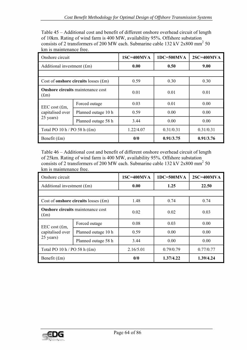
Cost Benefit Methodology for Optimal Design of Offshore Transmission Systems
Table 45 – Additional cost and benefit of different onshore overhead circuit of length of 10km. Rating of wind farm is 400 MW, availability 95%. Offshore substation consists of 2 transformers of 200 MW each. Submarine cable 132 kV 2x800 mm2 50 km is maintenance free. Onshore circuit 1SC=400MVA 1DC=500MVA 2SC=400MVA
Additional investment (£m) 0.00 0.50 9.00
Cost of onshore circuits losses (£m) 0.59 0.30 0.30
Onshore circuits maintenance cost (£m) 0.01 0.01 0.01
EEC cost (£m, capitalised over 25 years)
Forced outage 0.03 0.01 0.00
Planned outage 10 h 0.59 0.00 0.00
Planned outage 58 h 3.44 0.00 0.00
Total PO 10 h / PO 58 h (£m) 1.22/4.07 0.31/0.31 0.31/0.31
Benefit (£m) 0/0 0.91/3.75 0.91/3.76
Table 46 – Additional cost and benefit of different onshore overhead circuit of length of 25km. Rating of wind farm is 400 MW, availability 95%. Offshore substation consists of 2 transformers of 200 MW each. Submarine cable 132 kV 2x800 mm2 50 km is maintenance free. Onshore circuit 1SC=400MVA 1DC=500MVA 2SC=400MVA
Additional investment (£m) 0.00 1.25 22.50
Cost of onshore circuits losses (£m) 1.48 0.74 0.74
Onshore circuits maintenance cost (£m) 0.02 0.02 0.03
EEC cost (£m, capitalised over 25 years)
Forced outage 0.08 0.03 0.00
Planned outage 10 h 0.59 0.00 0.00
Planned outage 58 h 3.44 0.00 0.00
Total PO 10 h / PO 58 h (£m) 2.16/5.01 0.79/0.79 0.77/0.77
Benefit (£m) 0/0 1.37/4.22 1.39/4.24
Page 64 of 86
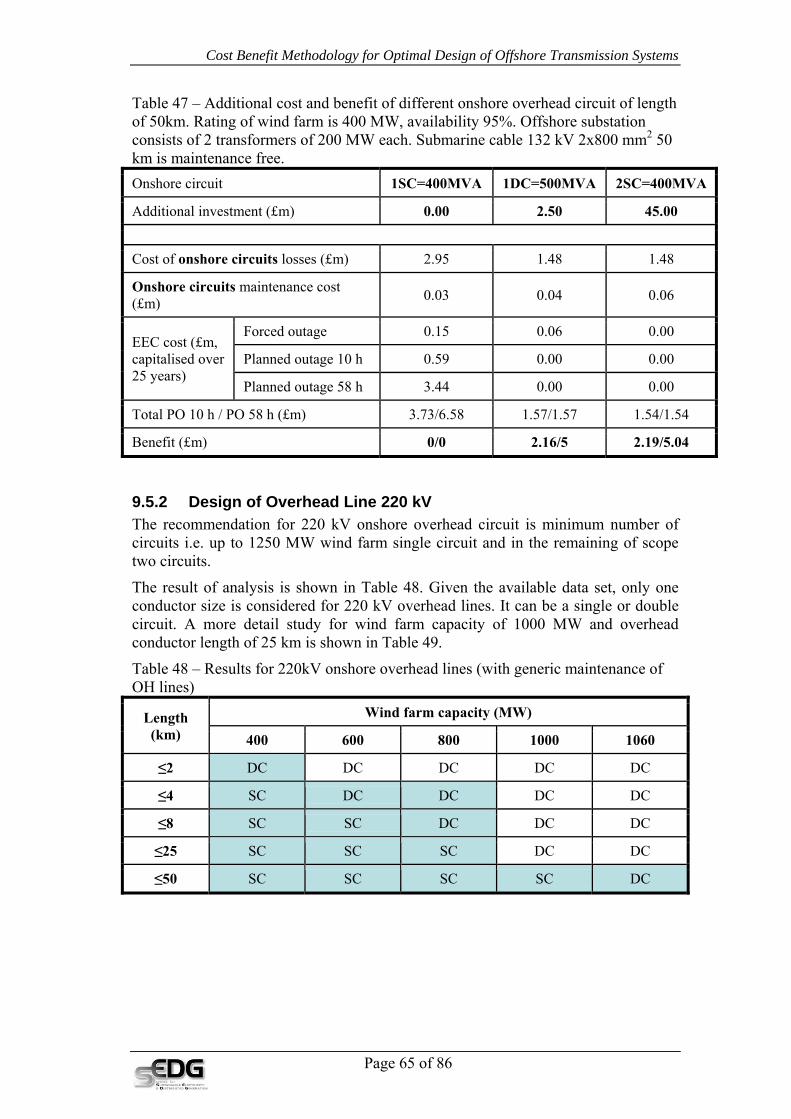
Cost Benefit Methodology for Optimal Design of Offshore Transmission Systems
Table 47 – Additional cost and benefit of different onshore overhead circuit of length of 50km. Rating of wind farm is 400 MW, availability 95%. Offshore substation consists of 2 transformers of 200 MW each. Submarine cable 132 kV 2x800 mm2 50 km is maintenance free. Onshore circuit 1SC=400MVA 1DC=500MVA 2SC=400MVA
Additional investment (£m) 0.00 2.50 45.00
Cost of onshore circuits losses (£m) 2.95 1.48 1.48
Onshore circuits maintenance cost (£m) 0.03 0.04 0.06
EEC cost (£m, capitalised over 25 years)
Forced outage 0.15 0.06 0.00
Planned outage 10 h 0.59 0.00 0.00
Planned outage 58 h 3.44 0.00 0.00
Total PO 10 h / PO 58 h (£m) 3.73/6.58 1.57/1.57 1.54/1.54
Benefit (£m) 0/0 2.16/5 2.19/5.04
9.5.2 Design of Overhead Line 220 kV The recommendation for 220 kV onshore overhead circuit is minimum number of circuits i.e. up to 1250 MW wind farm single circuit and in the remaining of scope two circuits.
The result of analysis is shown in Table 48. Given the available data set, only one conductor size is considered for 220 kV overhead lines. It can be a single or double circuit. A more detail study for wind farm capacity of 1000 MW and overhead conductor length of 25 km is shown in Table 49.
Table 48 – Results for 220kV onshore overhead lines (with generic maintenance of OH lines)
Length (km)
Wind farm capacity (MW)
400 600 800 1000 1060
≤2 DC DC DC DC DC
≤4 SC DC DC DC DC
≤8 SC SC DC DC DC
≤25 SC SC SC DC DC
≤50 SC SC SC SC DC
Page 65 of 86
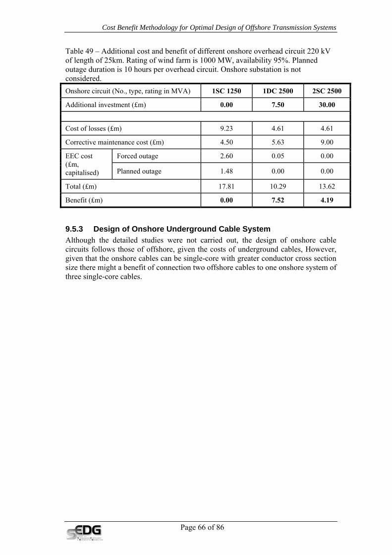
Cost Benefit Methodology for Optimal Design of Offshore Transmission Systems
Table 49 – Additional cost and benefit of different onshore overhead circuit 220 kV of length of 25km. Rating of wind farm is 1000 MW, availability 95%. Planned outage duration is 10 hours per overhead circuit. Onshore substation is not considered. Onshore circuit (No., type, rating in MVA) 1SC 1250 1DC 2500 2SC 2500
Additional investment (£m) 0.00 7.50 30.00
Cost of losses (£m) 9.23 4.61 4.61
Corrective maintenance cost (£m) 4.50 5.63 9.00
EEC cost (£m, capitalised)
Forced outage 2.60 0.05 0.00
Planned outage 1.48 0.00 0.00
Total (£m) 17.81 10.29 13.62
Benefit (£m) 0.00 7.52 4.19
9.5.3 Design of Onshore Underground Cable System Although the detailed studies were not carried out, the design of onshore cable circuits follows those of offshore, given the costs of underground cables, However, given that the onshore cables can be single-core with greater conductor cross section size there might a benefit of connection two offshore cables to one onshore system of three single-core cables.
Page 66 of 86
Page 67 of 86
Cost Benefit Methodology for Optimal Design of Offshore Transmission Systems
10. Rating Limits of a Single Circuit – Impact on Frequency Control
Connection of large wind farms, above 1320MW ((1320MW currently represents the maximum credible generation loss-MCGL), will have an impact on the cost of response14. The additional cost of response was determined by using the following approach.
1. Absolute load levels of the national demand in each half-hourly period of the year concurrent to the wind output are considered to determine the additional response requirements due to an instantaneous power loss of an offshore wind farm that is larger than 1320MW. This means that additional response requirements due to wind are assessed for each period (1/2-hr of the year) of the year.
iL
2. Using the annual wind profiles (and corresponding annual demand profile), the additional response requirements are determined for only those periods when the wind output is greater than the considered MCGL. w
iP
3. The system inertia effects at different loading conditions are included. This results in different response requirements even for same level of power loss at different loading conditions.
Having determined the additional response requirements w
iR due to wind during all periods (N) when wind level exceeds the MCGL, the additional response cost is determined by:
wiP
1
0.5wNi
gi g
RAdditional Response Cost C MSGr
η
=
⎧ ⎫⎪ ⎪= × × ×⎨ ⎬⎪ ⎪⎩ ⎭
∑
Where,
gCη is the cost of efficiency loss of the generator (unit) to provide response by operating at MSG (£/MW/hr)
gr is the total amount of reserve provided by each generator unit at its MSG level (MW)
MSG is minimum stable generation.
10.1 Rating Limit of a Single Converter Block in HVDC Applications
The reliability of the converter units and the maximum allowed frequency of power loss events affect the total capacity of the offshore wind farms and hence the rating
14 In this analysis we use a GB generation system model developed by SEDG (see “Value of fault ride through capability of wind generation in the UK”, www.sedg.ac.uk), used to support changes in Grid Code requirements associated with wind generation.
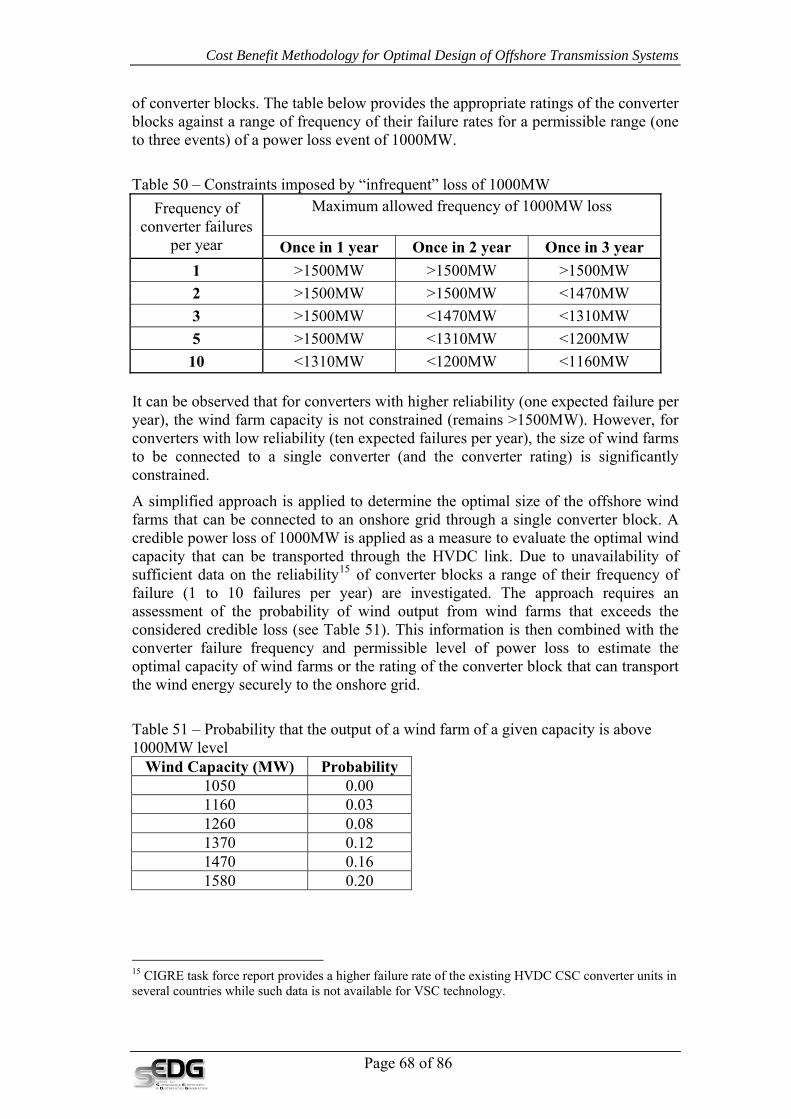
Page 68 of 86
Cost Benefit Methodology for Optimal Design of Offshore Transmission Systems
of converter blocks. The table below provides the appropriate ratings of the converter blocks against a range of frequency of their failure rates for a permissible range (one
three events) of a power loss event of 1000MW.
Tab aints impo
converter failures per year
Maximum allowed frequency of 1000MW loss
to
le 50 – ConstrFrequency of
sed by “infrequent” loss of 1000MW
Once in 1 year Once in 2 year Once in 3 year
1 >1500MW >1500MW >1500MW 2 >1500MW >1500MW <1470MW 3 >1500MW <1470MW <1310MW 5 >1500MW <1310MW <1200MW 10 <1310MW <1200MW <1160MW
It can be observed that for converters with higher reliability (one expected failure per year), the wind farm capacity is not constrained (remains >1500MW). However, for converters with low reliability (ten expected failures per year), the size of wind farms to be connected to a single converter (and the converter rating) is significantly
the converter block that can transport e wind energy securely to the onshore grid.
ability that the output of a wind farm of a given capacity is above 10
Wind Ca (MW) Probability
constrained.
A simplified approach is applied to determine the optimal size of the offshore wind farms that can be connected to an onshore grid through a single converter block. A credible power loss of 1000MW is applied as a measure to evaluate the optimal wind capacity that can be transported through the HVDC link. Due to unavailability of sufficient data on the reliability15 of converter blocks a range of their frequency of failure (1 to 10 failures per year) are investigated. The approach requires an assessment of the probability of wind output from wind farms that exceeds the considered credible loss (see Table 51). This information is then combined with the converter failure frequency and permissible level of power loss to estimate the optimal capacity of wind farms or the rating ofth
Table 51 – Prob
00MW level pacity1050 0.00 1160 0.03 1260 0.08 1370 0.12 1470 0.16 1580 0.20
15 CIGRE task force report provides a higher failure rate of the existing HVDC CSC converter units in several countries while such data is not available for VSC technology.

Page 69 of 86
Cost Benefit Methodology for Optimal Design of Offshore Transmission Systems
Examp
r year Probability of failure = 1/5 x 1/2 = 1/10 = 0.10
he ) around probability level of 0.1, which indicates that:
.08) x (1370-1260) + 1260 = 1310 MW
ind farm, grater than 1320MW, connected rough a single offshore HVDC circuit.
ind power output profiled represents 1500MW wind farm
m credible generation loss (MCGL) in the system was considered to be
esponse providing units are assumed to have the characteristics as given in Table 2.
T
le: For Converter reliability = 5 failures/year Permissible level of power (1000MW) loss = 2 pe
The appropriate size of wind farm can be determined through interpolation of tcapacity sizes (table 16 Size of wind capacity = (0.10-0.08)/(0.12-0
10.2 Rating Limit of a Single Circuit The objective of this study was to perform a cost benefit analysis to assess the economic suitability of providing additional response provision in order to manage instantaneous loss of a large offshore wth
Data: 1. Annual half-hourly generic GB wind data depicting diverse and non-diverse wind farms was used. Both wwith a 40% load factor.
2. Historical demand data of half-hourly averaged loads was used
3. Maximu1320MW
4. R5
able 52 – Characteristics of response providing unitsGeneric size of the unit providing response service 500 MW Minimum stable generation (MSG) level of the unit 250 MW Response provision by the unit at MSG 50 MW Fuel cost of the unit at full output 40 £/MWh Fuel cost of the unit at MSG 48 £/MWh Efficiency losses of the unit at MSG 20 %
It should be noted that the assumptions listed in table present an upper bound on additional response cost. The results of the evaluations of the response costs are resented in Table 53. p
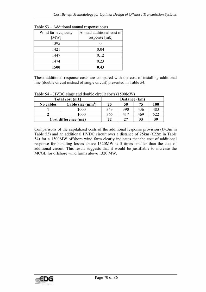
Page 70 of 86
Cost Benefit Methodology for Optimal Design of Offshore Transmission Systems
Ta nuWind Annual additional cost of
response [m£]
ble 53 – Additional anfarm capacity
al response costs
[MW] 1395 0 1421 0.04 1447 0.12 1474 0.23 1500 0.43
These additional response costs are compared with the cost of installing additional
ne (double circuit instead of single circuit) presented in Table 54.
Table 54 – HVDC singe and double circuit costs (1tal c Distance (km)
li
500MW)
To ost (m£) No cables Cable mm2) size ( 25 50 75 100
1 2000 343 390 436 483 2 1000 365 417 469 522
Cost difference (m£) 22 27 33 39 Comparisons of the capitalized costs of the additional response provision (£4.3m in Table 53) and an additional HVDC circuit over a distance of 25km (£22m in Table 54) for a 1500MW offshore wind farm clearly indicates that the cost of additional response for handling losses above 1320MW is 5 times smaller than the cost of additional circuit. This result suggests that it would be justifiable to increase the
CGL for offshore wind farms above 1320 MW.
M

Cost Benefit Methodology for Optimal Design of Offshore Transmission Systems
11. An Example Let us explore the options for connecting a wind farm of 300 MW to the onshore transmission system. A single platform with two transformers will be constructed. The distance to the shore connection requires that each cable is 50 km long. Find out the optimal direct connection arrangement.
Solution Required transformers rating is
STs ≥ X · PWF = 0.95 · 300 = 285 MVA
Therefore, two transformers of 150 MW are chosen and cost of platform and plant is:
PPC = 5 + (1 + 0.2 (2 – 2)) (20 + 25)/1000 · 2 · 150 = £18.5m
Various options in terms of voltage, number, and size of cables are investigated. Costs of cables per each case are given in the following Table
Voltage Number Size Rating Unit cost Length Capability Cost kV mm2 MVA m£/km km MW m£ 132 1 1000 217 0.59 50 216 29.5 132 2 500 169 0.42 50 168 42 220 1 500 279 0.59 50 273.5 29.5 220 1 630 308 0.625 50 301.5 31.25
Cost of compensation is given in the following Table
Voltage Number
Size Compensation (MVAr) Unit cost (m£/MVAr) Cost kV mm2 Offshore Onshore Offshore Onshore m£ 132 1 1000 0 20.9 0.025 0.015 0.3135132 2 500 0 21.8 0.025 0.015 0.6540220 1 500 0 54 0.025 0.015 0.8100220 1 630 0 60.4 0.025 0.015 0.9060
Estimation of cost of losses
The estimated cost of transformer losses is
( ) 7508760150100
6.0150
)12(30095.02012 2
2
⋅⋅⋅⋅⎥⎦
⎤⎢⎣
⎡⋅
⋅⋅+⋅= δCTL
which for non-diversified wind generation profile CTL is £3.70m and for diversified CTL is £3.06m.
The estimated cost of cables losses is
7508760130095.0501
2
⋅⋅⋅⎟⎠⎞
⎜⎝⎛
⋅⋅
⋅⋅⋅⋅= δV
rncCCL c
Page 71 of 86
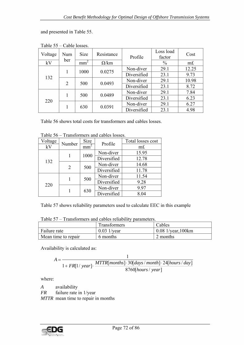
Page 72 of 86
Cost Benefit Methodology for Optimal Design of Offshore Transmission Systems
and presented in Table 55.
Table 55 – Cable losses.
Voltage Number
Size Resistance Profile Loss load
factor Cost
kV mm2 Ω/km % m£
132 1 1000 0.0275 Non-diver 29.1 12.25
Diversified 23.1 9.73
2 500 0.0493 Non-diver 29.1 10.98 Diversified 23.1 8.72
220 1 500 0.0489 Non-diver 29.1 7.84
Diversified 23.1 6.23
1 630 0.0391 Non-diver 29.1 6.27 Diversified 23.1 4.98
Table 56 shows total costs for transformers and cables losses.
Table 56 – Transformers and cables losses. Voltage Number Size Profile Total losses cost
kV mm2 m£
132 1 1000 Non-diver 15.95
Diversified 12.78
2 500 Non-diver 14.68 Diversified 11.78
220 1 500 Non-diver 11.54
Diversified 9.28
1 630 Non-diver 9.97 Diversified 8.04
Table 57 shows reliability parameters used to calculate EEC in this example
Table 57 – Transformers and cables reliability parameters. Transformers Cables Failure rate 0.03 1/year 0.08 1/year,100km Mean time to repair 6 months 2 months Availability is calculated as:
]/[8760]/[24]/[30][]/1[1
1
yearhoursdayhoursmonthdaysmonthsMTTRyearFR
A⋅⋅
⋅+=
where:
A availability FR failure rate in 1/year MTTR mean time to repair in months

Cost Benefit Methodology for Optimal Design of Offshore Transmission Systems
This gives the result that transformer availability is 0.9854 while availability of 50 km of cable is 0.9935.
For the case of one 132 kV cable of 1000 mm2 a capacity outage probability table is shown in Table 58. It also shows a constrained energy for a diversified wind generation profile.
Table 58 – Capacity outage probability table.
Capacity in (MW) Probability Energy constrained (MWh)
Expected energy constrained (MWh)
216 0.96471 33350 32173 150 0.02854 164848 4698 0 0.00674 998640 6691
Total 1.0000 Total 43609 Table 59 shows the EEC costs.
Table 59 – EEC cost. Voltage Numbe
r Size Profile EEC EEC cost
kV mm2 MWh m£
132 1 1000 Non-diver 108232 81.17
Diversified 43609 32.71
2 500 Non-diver 10934 8.20 Diversified 6470 4.85
220 1 500 Non-diver 19084 14.31
Diversified 11517 8.64
1 630 Non-diver 14666 11.00 Diversified 11440 8.58
Cost of transformers corrective maintenance is
( )[ ] mMCT 478.1£105.28760/2430603.0/12 =⋅⋅⋅⋅+=
while cost of cable corrective maintenance is
[ ] mMCc 199.0£255.0)8760/2430204.0/1/(1 =⋅⋅⋅⋅+=
which gives total cost of corrective maintenance of
mMCMCMC cT 68.1£=+=
for one cable and
mMCMCMC cT 88.1£2 =⋅+=
for two cables.
The total cost is given in Table 60.
Page 73 of 86

Cost Benefit Methodology for Optimal Design of Offshore Transmission Systems
Table 60 – Total cost. V N
o Size Profile PPC CC QC LC EECC MC Total
kV mm2 m£ m£ m£ m£ m£ m£ m£
132 1 1000 Non-diver 18.5 29.5 0.31 15.95 81.17 1.68 147.1
Diversified 18.5 29.5 0.31 12.78 32.71 1.68 95.5
2 500 Non-diver 18.5 42 0.65 14.68 8.20 1.88 85.9Diversified 18.5 42 0.65 11.78 4.85 1.88 79.7
220 1 500 Non-diver 18.5 29.5 0.81 11.54 14.31 1.68 76.3
Diversified 18.5 29.5 0.81 9.28 8.64 1.68 68.4
1 630 Non-diver 18.5 31.25 0.91 9.97 11.00 1.68 73.3Diversified 18.5 31.25 0.91 8.04 8.58 1.68 69.0
Notes: PPC platform and plant costs CC cables costs QC compensation costs LC losses costs EECC expected energy curtailed cost MC corrective maintenance cost The optimal solutions are shown in bold. It can be seen that the final solution is dependent on the footprint of wind farm. For a small wind farm footprint, i.e. the non-diversified wind generation profile can be assumed, the optimal solution is with one 220 kV 630 mm2 cable. In the other case, if diversified wind profile can be assumed, the optimal solution is with one 220 kV 500 mm2 cable.
Page 74 of 86

Cost Benefit Methodology for Optimal Design of Offshore Transmission Systems
12. Key Findings In this report, a cost-benefit based methodology was presented that is employed to determine an optimal design of the offshore transmission grid to connect offshore wind farms to onshore electricity networks. This methodology is used for the development of the new GBSQSS for Offshore Transmission Networks, as a part of the activities carried out by the GBSQSS sub-group of OTEG.
The developed cost benefit analysis was employed to find optimal trade offs between the following two broad categories of costs:
• cost of offshore transmission system investment, that is composed of: o costs of undersea cable network o cost of platform with associated equipment (transformers, reactive
compensation and switchgear) o cost of onshore circuits and substation and reactive compensation o capitalised cost of corrective maintenance and
• capitalised cost of expected constrained energy due to preventive and corrective maintenance and losses over the period of the asset life.
Based on evaluating the above two cost components for a spectrum of feasible offshore transmission system configurations with different levels of redundancy, we have identified optimal designs for undersea cable network and offshore platforms (including compensation both onshore and offshore), for a range of wind farms with ratings up to 1500 MW and for a range of offshore combined and open cycle gas turbines (GTs) with ratings up to 200 MW and various distances ranging from 25 km to 100 km. Furthermore, optimal designs of onshore circuits with length ranging from 1 to 50 km and onshore substations have been identified.
Specific recommendations The detailed cost-benefit analysis suggested that the design of offshore network systems could be separated into four main sections:
• the offshore platform (i.e. the AC transformer circuits and HVDC converters on the offshore platform);
• the offshore cable network (i.e. the transmission cable circuits linking the onshore network and the offshore platform);
• the onshore circuit if necessary • the onshore substation if necessary
Each of the four sections can be considered separately for single and multiple generation plants connections. However, coordination of preventive maintenance activities across offshore assets has to be considered simultaneously.
It should be noted from the results presented that each of the key input parameters has been tested to find the value at which the conclusion changes. A number of the key items of the input data to the cost benefit analysis have been tested (average repair times, cost of wind or gas turbines energy curtailed, etc.) to investigate at what
Page 75 of 86

Cost Benefit Methodology for Optimal Design of Offshore Transmission Systems
level these would change the design recommendations of the cost benefit analysis. A comprehensive set of more than 35,000 sensitivity studies was performed to propose the optimal design and to demonstrate the robustness of the recommendations made.
Offshore transmission network design for wind farms The following recommendations for offshore transmission system for wind farms are drawn:
• Minimum number of submarine cables with no redundancy. The total capacity of cables can be lower than the maximum export capacity of wind farms connected (see X factor in table below)
• Maximum rating of single transformer substation for offshore platform is 90MW. Minimum rating for multi-transformer substations is 50% of the wind farm rating and there is no impact of preventive maintenance
• Design of 132 kV overhead lines for wind farms to 400 MW is given in Table 61. For wind farms up to 1100 MW it is double circuit and above that is two double circuits. Design of 220 kV overhead lines are given in Table 62. Design of onshore underground cables will follow design of offshore subsea cables. However, there might be benefit of connecting two subsea cables to one onshore underground cable.
• Maximum rating of single transformer substation for onshore substation is 120-180MW
Table 61 – Results for 132kV onshore overhead lines (with generic maintenance of OH lines)
Length (km) Wind farm capacity (MW)
150 250 400
1 SC DC DC
10 SC SC/DC DC
25 SC SC DC
50 SC SC SC/DC
• SC – Single circuit • DC – Double circuit
Table 62 – Results for 220kV onshore overhead lines (with generic maintenance of OH lines)
Page 76 of 86

Cost Benefit Methodology for Optimal Design of Offshore Transmission Systems
Length (km)
Wind farm capacity (MW)
400 600 800 1000 1060
≤2 DC DC DC DC DC
≤4 SC DC DC DC DC
≤8 SC SC DC DC DC
≤25 SC SC SC DC DC
≤50 SC SC SC SC DC
As the diversity of wind power output was considered to potentially have an impact on the design of cable network, two extreme wind profiles are used:
• a non-diversified profile, characteristic for relatively small wind farms occupying relatively small geographical areas, and
• a diversified profile, characteristic for relatively large wind farms occupying relatively large areas. In this case, due to the dispersed locations of the wind generators, statistically there is a relatively low probability that full output of all individual wind generators will be available at any given time.
Offshore platform
The quantitative assessments demonstrated that offshore platform capacity should be about 95% of the maximum export capacity of the wind farm connected. Furthermore, for wind farms with a capacity of 90MW or greater, following an outage (planned or unplanned) of any offshore platform transformer, there should be, at a minimum, 50% of the installed platform transformer capacity remaining.
Offshore Cable Network
For cable networks, the total optimal capacity installed can be lower than the maximum export capacity of the wind farm connected, due to the cost of installing offshore transmission assets to full capacity (X factor in table below). For the non-diversified wind profile (appropriate for relatively small wind farms, occupying small geographical areas) the installed network capacity should be above 95% of the maximum output of the wind farm, while in the case of a diversified wind profile (appropriate for relatively large wind farms occupying relatively large areas) the installed network capacity should be above 90% of the maximum output of the wind farm. In cases where this value requires an additional cable to be installed, consideration should be given to installation of network capacity below 95% for a non-diversified profile and below 90% for diversified profiles. The optimal values of the X factor will be a function of the distance as shown in the table below.
X factor (%) Cable length (km)
Page 77 of 86
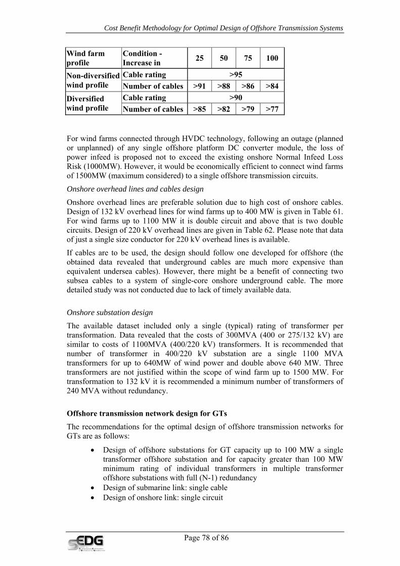
Cost Benefit Methodology for Optimal Design of Offshore Transmission Systems
Wind farm profile
Condition - Increase in 25 50 75 100
Non-diversified wind profile
Cable rating >95Number of cables >91 >88 >86 >84
Diversified wind profile
Cable rating >90Number of cables >85 >82 >79 >77
For wind farms connected through HVDC technology, following an outage (planned or unplanned) of any single offshore platform DC converter module, the loss of power infeed is proposed not to exceed the existing onshore Normal Infeed Loss Risk (1000MW). However, it would be economically efficient to connect wind farms of 1500MW (maximum considered) to a single offshore transmission circuits.
Onshore overhead lines and cables design
Onshore overhead lines are preferable solution due to high cost of onshore cables. Design of 132 kV overhead lines for wind farms up to 400 MW is given in Table 61. For wind farms up to 1100 MW it is double circuit and above that is two double circuits. Design of 220 kV overhead lines are given in Table 62. Please note that data of just a single size conductor for 220 kV overhead lines is available.
If cables are to be used, the design should follow one developed for offshore (the obtained data revealed that underground cables are much more expensive than equivalent undersea cables). However, there might be a benefit of connecting two subsea cables to a system of single-core onshore underground cable. The more detailed study was not conducted due to lack of timely available data.
Onshore substation design
The available dataset included only a single (typical) rating of transformer per transformation. Data revealed that the costs of 300MVA (400 or 275/132 kV) are similar to costs of 1100MVA (400/220 kV) transformers. It is recommended that number of transformer in 400/220 kV substation are a single 1100 MVA transformers for up to 640MW of wind power and double above 640 MW. Three transformers are not justified within the scope of wind farm up to 1500 MW. For transformation to 132 kV it is recommended a minimum number of transformers of 240 MVA without redundancy.
Offshore transmission network design for GTs The recommendations for the optimal design of offshore transmission networks for GTs are as follows:
• Design of offshore substations for GT capacity up to 100 MW a single transformer offshore substation and for capacity greater than 100 MW minimum rating of individual transformers in multiple transformer offshore substations with full (N-1) redundancy
• Design of submarine link: single cable • Design of onshore link: single circuit
Page 78 of 86

Cost Benefit Methodology for Optimal Design of Offshore Transmission Systems
• Design of onshore substation: single transformer The impact of preventive maintenance is also analysed including coordination of maintenance of different network assets. It has been concluded that for design of offshore infrastructure for GT generation there is no impact of preventive maintenance outages.
Page 79 of 86

Cost Benefit Methodology for Optimal Design of Offshore Transmission Systems
13. References ILEX Energy and Strbac, G. (Oct. 2002), Quantifying the system costs of additional renewables 2020, http://www.dti.gov.uk/energy/developep/080scar_report_v2_0.pdf
Shakoor, A. (2005): Security and Cost Evaluation of Power Generation Systems with Intermittent Energy Sources, PhD thesis, The University of Manchester
R. Billinton, and R.N. Allan, “Reliability of Engineering Systems: Concepts and Techniques”, second edition, Plenum Publishing, New York, 1992
R. Billinton, and R.N. Allan, “Reliability of Power Systems”, second edition, Plenum Publishing, New York, 1996
Page 80 of 86
Page 81 of 86
Cost Benefit Methodology for Optimal Design of Offshore Transmission Systems
14. Appendix – Equipments and Cost Data The information for cost calculation is available on the GBSQSS sub-group webpage16. For completeness, they are repeated here together with the interpolated and/or extrapolated values.
Two wind farm profiles are used: non-diversified and diversified. Both profiles have 40% load factors. Availability of wind power is assumed 95%.
Assumed average value of cost of energy is £75/MWh. Two extreme values are also investigated £50/MWh and £100/MWh.
HVAC platform cost consists of fixed cost of £5m per platform and variable costs of £20/kVA if two transformers are on a platform. If just one transformer is on a platform variable cost is reduced to 80%. For more than two transformers variable cost is increased for 20% for each additional transformer. Please note that the total rating power of all transformers on the platform remain the same. Cost of AC plant is £25/kVA if two transformers are on a platform. Similarly, to the cost of plant is increased by 20% for third and each successive transformer or decreased by 20% for just one transformer on a platform. For clarity, the previous note still applies. The repair cost of transformers is £2.5m.
The electrical parameters of AC transformers are as follows: load losses 0.6%, losses factor (load losses / no-load losses) 20 and reactance 15%. Maximum rating of an AC transformer is assumed 500 MVA
HVDC VSC platform and plant cost consists of fixed costs £25m per platform and variable costs of £110/kW for two converters on a platform. The cost is linearly adjusted for different number of converters while total rated power is kept unchanged. It is increased for 20% for third and further 20% per each successive converter and decreased for 20% for just one converter on a platform. HVDC VSC converter average repair cost is £0.5m per repair.
The load and no-load losses of HVDC VSC converters are each 0.8%.
Cost of offshore compensation is £25/kVAr and onshore £15/kVAr.
Cost of AC cables are given in Table 63 and of HVDC in Table 64. Electrical parameters of AC cables are given in Table 65 and of HVDC in Table 66. Cable maintenance cost is £0.5m.
16 http://www.dti.gov.uk/energy/sources/renewables/policy/offshore-transmission/offshore-transmission-experts-group/page31187.html

Cost Benefit Methodology for Optimal Design of Offshore Transmission Systems
Table 63 – HVAC cables cost. Voltage
(kV) Cable size
(mm2) Cables cost (£/m) – 3 core or set of three single core
Supply Lay and Bury Total
132
500 240 180 420 630 275 185 460 800 310 190 500
1000 390 200 590
220
500 390 200 590 630 415 210 625 800 440 220 660
1000 460 230 690
400
800 860 540 1400 1000 995 555 1550 1200 1130 570 1700 1400 1265 585 1850 1600 1400 600 2000 2000 1535 615 2150
Table 64 – HVDC cables cost.
Voltage (kV)
Cable size (mm2)
Cables cost (£/m) –set of two DC single core (VSC)
Supply Lay and Bury Total
150
1000 310 360 670 1200 360 370 730 1400 405 380 785 1600 450 390 840 2000 500 400 900
300
1000 440 415 855 1200 510 430 940 1400 575 440 10151600 640 450 10902000 710 465 1175
Table 65 – Electrical parameters of HVAC cables
Voltage Cable size No
cores
AC resistance Inductance Capacitance Steady state rating
kV mm2 mΩ/km mH/km nF/km A MVA
132
500 3 49.3 0.387 192 739 169 630 3 39.5 0.372 209 818 187 800 3 32.4 0.364 217 888 203
1000 3 27.5 0.351 238 949 217
220
500 3 48.9 0.437 136 732 279 630 3 39.1 0.415 151 808 308 800 3 31.9 0.4 163 879 335
1000 3 27 0.386 177 942 359
400
800 1 31.4 0.54 130 870 603 1000 1 26.5 0.52 140 932 646 1200 1 22.1 0.49 170 986 683 1400 1 18.9 0.47 180 1015 703 1600 1 16.6 0.46 190 1036 718 2000 1 13.2 0.44 200 1078 747
Page 82 of 86

Cost Benefit Methodology for Optimal Design of Offshore Transmission Systems
Table 66 – Electrical parameters of HVDC cables
Voltage Cable size
DC resistance Steady state rating
kV mm2 mW/km A MW
150
1000 22.4 1644 4931200 19.2 1791 5371400 16.5 1962 5891600 14.4 2123 6372000 11.5 2407 722
300
1000 22.4 1644 9861200 19.2 1791 10751400 16.5 1962 11771600 14.4 2123 12742000 11.5 2407 1444
Reliability parameters used in calculation are summarised in Table 67.
Table 67 – Reliability parameters Element Failure rate Mean time to repair*
Transformers 0.03 (1/year) 3 and 6 months Converters 0.12 (1/year) 1 month Cables 0.08 (1/year,100km) 2 months
* It is assumed that each month has 30 days
Costs of ‘small’ transformers are given in Table 68.
Table 68 – Cost of ‘small’ transformers Transformer rating (MVA) 30 45 60 90 120 Base cost (m£) 0.420 0.490 0.600 0.740 0.930
Page 83 of 86

Cost Benefit Methodology for Optimal Design of Offshore Transmission Systems
14.1 Update of Equipment and Cost Data
14.1.1 New Cost Data Table 69 – AC submarine cables costs
Voltage (kV)
Cable size (mm2)
Cables cost (£/m) – 3 core
Supply Lay and Bury Total
132
500 335 300 635
630 385 300 685
800 495 300 795
1000 560 300 860
220
500 515 300 815
630 550 300 850
800 675 300 975
1000 700 300 1000
Table 70 – AC underground cables costs
Voltage (kV)
Cable size (mm2)
Cables cost (£/m) – 3 core
Supply Lay and Bury Total
132
500 335 300+255 890
630
800 495 300+322 1117
1000
1200 495+130 300+300? 1268
220
500 515 300+300 1115
630 550 300+300 1150
800 675 300+300 1275
1000 700 300+300 1300
Table 71 – Base cost of 132 /33 kV transformers Transformer rating (MVA) 30 45 60 90 120
Base cost (m£) 0.530 0.610 0.750 0.930 1.160
Page 84 of 86
Cost Benefit Methodology for Optimal Design of Offshore Transmission Systems
14.1.2 Further CBA dataset for Inclusion of Preventive Maintenance General Energy cost
Winter - £45/MWh Summer - £35/MWh ROC value - £30/MWh
Wind farm output Load factor during forced outages – 40% Load factor during planned outages – 24%
Limits to analysis Up to 100km from the 1st onshore substation Up to 50km onshore OHL section Up to 1500MW wind farm capacity Up to 200MW gas turbine capacity
Transformers Offshore transformers (for revised work)
Losses: load 0.6%, no-load 0.03% Failure rate 3% Mean Time To Repair 6 months Repair cost per fault - £2.5m Cost - £29/kVA (for two transformers on a platform) 20% additional cost for third and each successive transformer 20% decrease in cost for just one transformer on a platform
Platform cost - £5m per platform plus £23/kVA (for two transformers on a platform) 20% additional cost for each additional transformer
Onshore transformers Failure rate 2% - (Source - CIGRE WG 12.05 concluded the average failure rate for units installed on systems operating at voltage lower than 700 kV)
Mean time to repair 2 months (Source - National Grid) Maintenance requirements – 5 days per annum (Source - National Grid) Electrical parameters; (Source - National Grid) 400/220 - X=1.6% R=0.02% on 100MVA base (assumed the same as 400/275 unit) 400/132 - X=8% R=0.14% on 100MVA base
220/132 - X=9% R=0.16% on 100MVA base (assumed the same as 275/132 unit)
Cost; (Source - National Grid) 400/220 (assumed the same as 400/275 unit) £2.7m (1100MVA which is Maximum permissible)
400/132 £2.5m (240MVA – Maximum permissible 460MVA) 275/132 £2.1m (240MVA – Maximum permissible 460MVA) 0.12% of cost per MVA change in rating above 240MVA up to maximum permissible HV bay for transformer, to include CB: (Source - National Grid) 400kV – £1.8m 220 / 275kV - £1.6m
Overhead lines Electrical parameters;
R = 2.9x10⁻³% on 100MVA base X = 0.386% on 100MVA base
Reliability;
Page 85 of 86
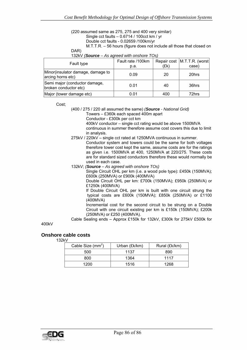
Cost Benefit Methodology for Optimal Design of Offshore Transmission Systems
Page 86 of 86
(220 assumed same as 275, 275 and 400 very similar) Single cct faults – 0.6714 / 100cct km / yr Double cct faults - 0.02659 /100km/yr M.T.T.R. – 56 hours (figure does not include all those that closed on DAR)
132kV (Source – As agreed with onshore TOs)
Fault type Fault rate /100km p.a.
Repair cost (£k)
M.T.T.R. (worst case)
Minor(insulator damage, damage to arcing horns etc) 0.09 20 20hrs
Semi major (conductor damage, broken conductor etc) 0.01 40 36hrs
Major (tower damage etc) 0.01 400 72hrs Cost;
(400 / 275 / 220 all assumed the same) (Source - National Grid) Towers – £360k each spaced 400m apart Conductor - £300k per cct km
400kV conductor – single cct rating would be above 1500MVA continuous in summer therefore assume cost covers this due to limit in analysis.
275kV / 220kV – single cct rated at 1250MVA continuous in summer. Conductor system and towers could be the same for both voltages therefore tower cost kept the same, assume costs are for the ratings as given i.e. 1500MVA at 400, 1250MVA at 220/275. These costs are for standard sized conductors therefore these would normally be used in each case.
132kV; (Source – As agreed with onshore TOs) Single Circuit OHL per km (i.e. a wood pole type): £450k (150MVA); £600k (250MVA) or £900k (400MVA) Double Circuit OHL per km: £700k (150MVA); £950k (250MVA) or £1250k (400MVA) If Double Circuit OHL per km is built with one circuit strung the typical costs are £600k (150MVA); £850k (250MVA) or £1100 (400MVA) Incremental cost for the second circuit to be strung on a Double Circuit with one circuit existing per km is £150k (150MVA); £200k (250MVA) or £250 (400MVA).
Cable Sealing ends – Approx £150k for 132kV, £300k for 275kV £500k for 400kV Onshore cable costs 132kV
Cable Size (mm2) Urban (£k/km) Rural (£k/km) 500 1137 890 800 1364 1117 1200 1516 1268