Embed Size (px)
Citation preview
Quantification of the effects on greenhouse gas emissions of policies and measures Reference: ENV.C.1/SER/2007/0019
Methodologies Report
A final report to the European Commission
Restricted Commercial ED05611
December 2009

Restricted – Commercial ENV.C.1/SER/2007/0019 AEA/ED05611/Methodologies Report/Issue1
i AEA
Title Quantification of the effects on greenhouse gas emissions of policies and measures: Methodologies Report
Customer European Commission
Customer reference ENV.C.1/SER/2007/0019
Confidentiality, copyright and reproduction
Copyright AEA Technology plc
All rights reserved Enquiries about copyright and reproduction should be addressed to the Commercial Manager, AEA Technology plc
File reference ED05611
Reference number ED05611
Daniel Forster AEA group The Gemini Building Fermi Avenue Harwell International Business Centre Didcot OX11 0QR
Tel: 0870 190 6474 Fax: 0870 190 6318
AEA is a business name of AEA Technology plc
AEA is certificated to ISO9001 and ISO14001
Author Name Daniel Forster, Angela Falconer (AEA) Marco Buttazoni, James Greenleaf (Ecofys) Wolfgang Eichhammer (Fraunhofer ISI)
ACEA: Jonathan Köhler (Fraunhofer ISI); Appliances: Stefano Faberi (ISIS), Wolfgang Eichhammer (Fraunhofer ISI); Biofuels: Wolfgang Eichhammer (Fraunhofer ISI), Felipe Toro (BSR Sustainability); CAP: Daniel Forster (AEA); CHP: Robert Harmsen (Ecofys); EPBD: Stefano Faberi (ISIS), Wolfgang Eichhammer (Fraunhofer ISI); ETS: Joachim Schleich, Frank Sensfuss, Wolfgang Eichhammer (all Fraunhofer ISI); Fgas: JanMartin Rhiemeier (Ecofys); IPPC: Angela Falconer (AEA); Landfill: Michael Harfoot (AEA); Nitrates: Daniel Forster (AEA); RESE: Mario Ragwitz (Fraunhofer ISI); WID: Michael Harfoot (AEA)

ENV.C.1/SER/2007/0019 Restricted – Commercial AEA/ED05611/Methodologies Report/Issue1
ii AEA
Table of contents
Glossary ................................................................................................................... iv
1 Introduction ...................................................................................................... 1 2 Expost evaluation: general methodological issues..................................... 2
2.1 Overview of expost evaluation.......................................................................................2
2.2 Methodological challenges for an expost evaluation ......................................................3
2.3 Type of methodologies ...................................................................................................9
2.4 Discussion and conclusions .........................................................................................16
3 Proposed methodological approach for the expost evaluation of EU Climate Change Policies........................................................................................ 17
3.1 Selecting a methodological framework .........................................................................17
3.2 Overall evaluation of methodologies.............................................................................22
3.3 The methodological framework.....................................................................................22
3.4 Implementation of the framework..................................................................................25
4 Guidelines for the ExPost Evaluation of EU Directives ............................. 40 4.1 Guidelines for the Expost impact assessment of ECCP Measures on the Member State
level: Renewable Electricity (RESE) Directive.........................................................................42
4.2 Guidelines for the Expost impact assessment of ECCP Measures on the Member State
level: Biofuels Directive ...........................................................................................................45
4.3 Guidelines for the Expost impact assessment of ECCP Measures on the Member State
level: CHP Directive ................................................................................................................48
4.4 Guidelines for the Expost impact assessment of ECCP Measures on the Member State
level: Voluntary Agreements for Cars between the European Commission and ACEA, JAMA
and KAMA...............................................................................................................................52
4.5 Guidelines for the Expost impact assessment of ECCP Measures on the Member State
level: Landfill Directive.............................................................................................................61
4.6 Guidelines for the Expost impact assessment of ECCP Measures on the Member State
level: Waste Incineration Directive...........................................................................................68
4.7 Guidelines for the Expost impact assessment of ECCP Measures on the Member State
level: reform of the sheep and goat meat regime and beef sector premia under CAP...............73
4.8 Guidelines for the Expost impact assessment of ECCP Measures on the Member State
level: IPPC Directive ...............................................................................................................81
4.9 Guidelines for the Expost impact assessment of ECCP Measures on the Member State
level: Nitrates Directive............................................................................................................87
4.10 Guidelines for the Expost impact assessment of ECCP Measures on the Member State
level: example for the F Gas Regulation.................................................................................93
4.11 Guidelines for the Expost impact assessment of ECCP Measures on the Member State
level: example for the Emissions Trading Directive ..................................................................99
Restricted – Commercial ENV.C.1/SER/2007/0019 AEA/ED05611/Methodologies Report/Issue1
iii AEA
4.12 Guidelines for the Expost impact assessment of ECCP Measures on the Member State
level: example for the Energy Performance of Buildings Directive..........................................108
4.13 Guidelines for the Expost impact assessment of ECCP Measures on the Member State
level: example for the Labelling of household appliances.......................................................113
5 Future Developments....................................................................................120 6 References.....................................................................................................122 Appendix I: Working Paper on methodological issues related to the calculation of emission factors................................................................................................123
1.1 Introduction................................................................................................................123
1.2 Methodological issues for emission factors related to electricity generation.................123
Annex 1: Structure of the PowerACE model .......................................................129
Appendix II: Case Study application of Tier 3 methodology .............................130

ENV.C.1/SER/2007/0019 Restricted – Commercial AEA/ED05611/Methodologies Report/Issue1
iv AEA
Glossary
Autonomous development
Autonomous development can describe a range of interrelated factors that influence the counterfactual trend in emissions (e.g. technological innovation), but are not directly attributable to the policy under investigation.
Bottomup model Bottomup models represent reality by aggregating characteristics of specific activities and processes, considering technological, engineering and cost details. See also topdown model.
CAP Common Agricultural Policy of the European Union Counterfactual The most likely situation that would have occurred without the policy
intervention; the ‘reference case’. Any evaluation of a policy’s effects should be made relative to what would otherwise have happened.
Econometric model
A type of topdown model, they relate energy demand to other variables such as prices and income or output levels (based on past trends). They represent the behaviour of the economy through relationships based on key economic factors such as GDP.
Effectiveness The extent to which the policy objectives have been achieved, and therefore the amount of GHG savings that can be attributed to the policy.
Efficiency The amount of GHG savings achieved per total cost incurred. Emission factor Number representing emissions of a greenhouse gas per unit of activity, for
example, kilograms of CO2 emitted per tonne of fuel combusted. See also conversion factor.
Endogenous A factor generated from within the system or model, the opposite of exogenous.
Ex ante evaluation
An evaluation conducted before the implementation of a policy intervention, where impacts are based on future projections. Also known as ‘policy appraisal’.
Ex post evaluation
An evaluation conducted during or after completion of a policy intervention, where impacts are based on historical evidence.
Exogenous An exogenous variable is one that comes from outside the model, but which in reality has a direct effect on the results that the model is trying to estimate. For example, changes in consumer preferences or worldwide commodity prices on emissions levels. Hence, where such exogenous variables are not adequately accounted for by the model they will be implicitly included on the results, and lead to over/underestimation of the impact of the endogenous variables.
Freeriders Beneficiaries of subsidy or other policy intervention, who would have made the desired change (e.g. purchase of improved technology) even in the absence of the policy. Also known as deadweight loss.
General equilibrium model
Describes the whole economy, including all markets (labour market, markets for investment goods etc); the model assume that all economic agents optimise their behaviour, and price mechanisms work to clear all markets. Partial equilibrium models describe demand and supply behaviours in one market at a time, ignoring the effects on other markets.
GHG Greenhouse gases Multiplier effect Where the initial carbon/energy saving effect of a policy is enhanced further,
for example, due to a market transformation (e.g. implementation of a measure without any further involvement from the authorities or agencies) or further innovation.
PAM a policy or measure (hence PAMs: policies and measures) Policy theory Also termed “intervention logic”, the concept and underlying assumptions
about how the policy achieves its objectives (e.g. reduced energy consumption), and how achievement of the objectives contributes to the attainment of the goal (e.g. GHG savings). Establishing the policy theory is central to an evaluation of the policy’s effectiveness.
Rebound effect A price effect: after implementation of more efficient technologies or practices, part of the savings is taken back for more intensive or other

Restricted – Commercial ENV.C.1/SER/2007/0019 AEA/ED05611/Methodologies Report/Issue1
v AEA
consumption. Direct rebound effect: if energy efficiency improvements lead to a price decrease of the energy ‘service’ (the utility obtained from consuming energy, e.g. vehicle km in transport sector, room heating in residential sector), then this will lead to an increase in consumption of that service. Indirect rebound effect: consumers spend released income (from a price decrease for an energy service) on other goods and services, the production of which leads to an increase in energy consumption.
Reference technology
The technology that is assumed to be used in the absence of the policy, and therefore used in the counterfactual scenario. An alternative technology (e.g. gas turbines) to that being stimulated by the policy (e.g. renewable energy).
Topdown model Topdown models represent reality by applying macroeconomic theory, econometric and optimization techniques to aggregate economic variables. Using historical data on consumption, prices, incomes, and factor costs, top down models assess final demand for goods and services, and supply from main sectors, like the energy sector, transportation, agriculture, and industry. Complex topdown models can be divided into two main categories: macroeconometric/econometric and general equilibrium. However, simpler topdown models also utilise more basic indicatorbased approaches. See also bottomup model.


Restricted – Commercial ENV.C.1/SER/2007/0019 AEA/ED05611/Methodologies Report/Issue1
AEA 1
1 Introduction This report has been prepared for the European Commission under the contract ENV.C.1/SER/2007/0019.
The primary aim of the report is to describe the methodologies that have been developed during the project to evaluate, ex post, the impact of selected EU Climate Change Policies and Measures (PAMS) on greenhouse gas (GHG) emissions. The secondary aim of the document is to provide guidance to Member State representatives on expost evaluation, and to provide references and tools that facilitate the implementation of a consistent approach across the EU27 countries.
The focus of the guidance is on approaches to evaluate the effectiveness of the policies and measures. Evaluating the efficiency of policies is another important component of policy evaluation, but is only considered to a limited extent within these guidelines.
The document is organised in the following sections:
• Section 2 discusses the broad methodological issues associated with expost evaluation, illustrating the main approaches available and their strengths and weaknesses
• Section 3 describes the methodological framework proposed for the evaluation of EU Climate Change Policies, providing explanation of key decisions informing the approach and the actual guidelines for the policy evaluation of individual directives
• Section 4 includes policy evaluation guidelines for the following EU climate change policies 1 :
o RESE Electricity production from renewable energy sources (Dir 2001/77/EC) o Biofuels Directive (Dir 2003/30/EC) o Promotion of cogeneration (Dir 2004/8/EC) o Voluntary agreement with car manufacturers to reduce CO2 emissions (ACEA, KAMA,
JAMA) o Landfill Directive (Dir 1999/31/EC) o Waste incineration Directive (Dir 2000/76/EC)EU Emissions trading scheme (Dir
2003/87/EC) (including the linking Directive) o Common rules for direct support schemes under CAP (Regulation (EC) No 1782/2003) o Integrated pollution prevention and control (IPPC) (Dir 96/61/EC) o Nitrates Directive (Dir 91/676/EEC) o FGas Regulation (EC No 842/2006) on certain fluorinated greenhouse gases o EU Emissions Trading Scheme Directive (2003/87/EC) o Energy performance of buildings (Dir 2002/91/EC) o Energy labelling of household appliances (Dir 2003/66/EC, 2002/40/EC, 2002/31/EC,
99/9/EC, 98/11/EC, 96/89/EC, 96/60/EC)
• Section 5 includes concluding remarks on the role the guidelines could play in EU and MS climate change policy and on the their possible future evolution
The following Appendices are also included in the document:
• Appendix I:Working Paper on methodological issues related to the calculation of emission factors
• Appendix II: Case study applications of a Tier 3 methodology. o RESE Electricity production from renewable energy sources (Dir 2001/77/EC) o EU Emissions trading scheme (Dir 2003/87/EC) (including the linking Directive) o Voluntary agreement with car manufacturers to reduce CO2 emissions (ACEA, KAMA,
JAMA) o Biofuels Directive (Dir 2003/30/EC) o Energy performance of buildings (Dir 2002/91/EC) o Energy labelling of household appliances (Dir 2003/66/EC, 2002/40/EC, 2002/31/EC,
99/9/EC, 98/11/EC, 96/89/EC, 96/60/EC)
1 The Energy Services Directive is not included within this subject as it is subject to detailed work on evaluation methodologies under the EMEEES project http://www.evaluateenergysavings.eu/emeees/en/home/index.php
ENV.C.1/SER/2007/0019 Restricted – Commercial AEA/ED05611/Methodologies Report/Issue1
2 AEA
2 Expost evaluation: general methodological issues
This section provides a general description of what is meant by expost evaluation, highlighting key goals and concepts. Critical issues and the main approaches for expost evaluation activities are also discussed. The discussion presented in this section is relevant for the expost evaluation of any policy, not just climate change policies. Examples relating to ECCP (European Climate Change Programme) policies, and climate change policies in general, will be utilised to illustrate specific issues and approaches.
The section provides background information for section 3, where the specific methodological framework developed for the evaluation of the EU climate change policies is described.
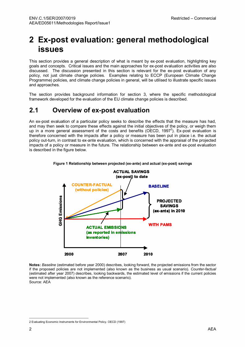
2.1 Overview of expost evaluation An expost evaluation of a particular policy seeks to describe the effects that the measure has had, and may then seek to compare these effects against the initial objectives of the policy, or weigh them up in a more general assessment of the costs and benefits (OECD, 1997 2 ). Expost evaluation is therefore concerned with the impacts after a policy or measure has been put in place i.e. the actual policy outturn, in contrast to exante evaluation, which is concerned with the appraisal of the projected impacts of a policy or measure in the future. The relationship between exante and expost evaluation is described in the figure below.
Figure 1 Relationship between projected (exante) and actual (expost) savings
ACTUAL SAVINGS (expost) to date
COUNTERFACTUAL (without policies)
ACTUAL EMISSIONS (as reported in emissions inventories)
2000 2010
GHG Emission
s
2007
BASELINE
WITH PAMS
PROJECTED SAVINGS
(exante) in 2010
ACTUAL SAVINGS (expost) to date
COUNTERFACTUAL (without policies)
ACTUAL EMISSIONS (as reported in emissions inventories)
ACTUAL SAVINGS (expost) to date
COUNTERFACTUAL (without policies)
ACTUAL EMISSIONS (as reported in emissions inventories)
ACTUAL EMISSIONS (as reported in emissions inventories)
2000 2010
GHG Emission
s
2007
BASELINE
WITH PAMS
PROJECTED SAVINGS
(exante) in 2010
2000 2010
GHG Emission
s
2007 2007
BASELINE
WITH PAMS
PROJECTED SAVINGS
(exante) in 2010
PROJECTED SAVINGS
(exante) in 2010
Notes: Baseline (estimated before year 2000) describes, looking forward, the projected emissions from the sector if the proposed policies are not implemented (also known as the business as usual scenario). Counterfactual (estimated after year 2007) describes, looking backwards, the estimated level of emissions if the current policies were not implemented (also known as the reference scenario). Source: AEA
2 Evaluating Economic Instruments for Environmental Policy. OECD (1997)
Restricted – Commercial ENV.C.1/SER/2007/0019 AEA/ED05611/Methodologies Report/Issue1
AEA 3
Expost evaluation should be considered an integral part of the policy development cycle, since the findings from an evaluation can provide valuable insights to improve the effectiveness and efficiency of future polices. The OECD identifies the main benefits associated with more extensive evaluation of environmental policies as follows:
• Evaluation evidence on the performance of policy instruments could help to improve the administration of current policy, and can contribute to a process of policy reappraisal, modification and improvement in the light of experience.
• Evaluations can also improve the choice of instruments in future policy, by demonstrating how different instruments perform in specific contexts. Countries may be able to learn from the practical experience of policy approaches adopted elsewhere.
• Evaluation may also contribute to better communication with stakeholders and the public about the purpose, operation and effects of policy.
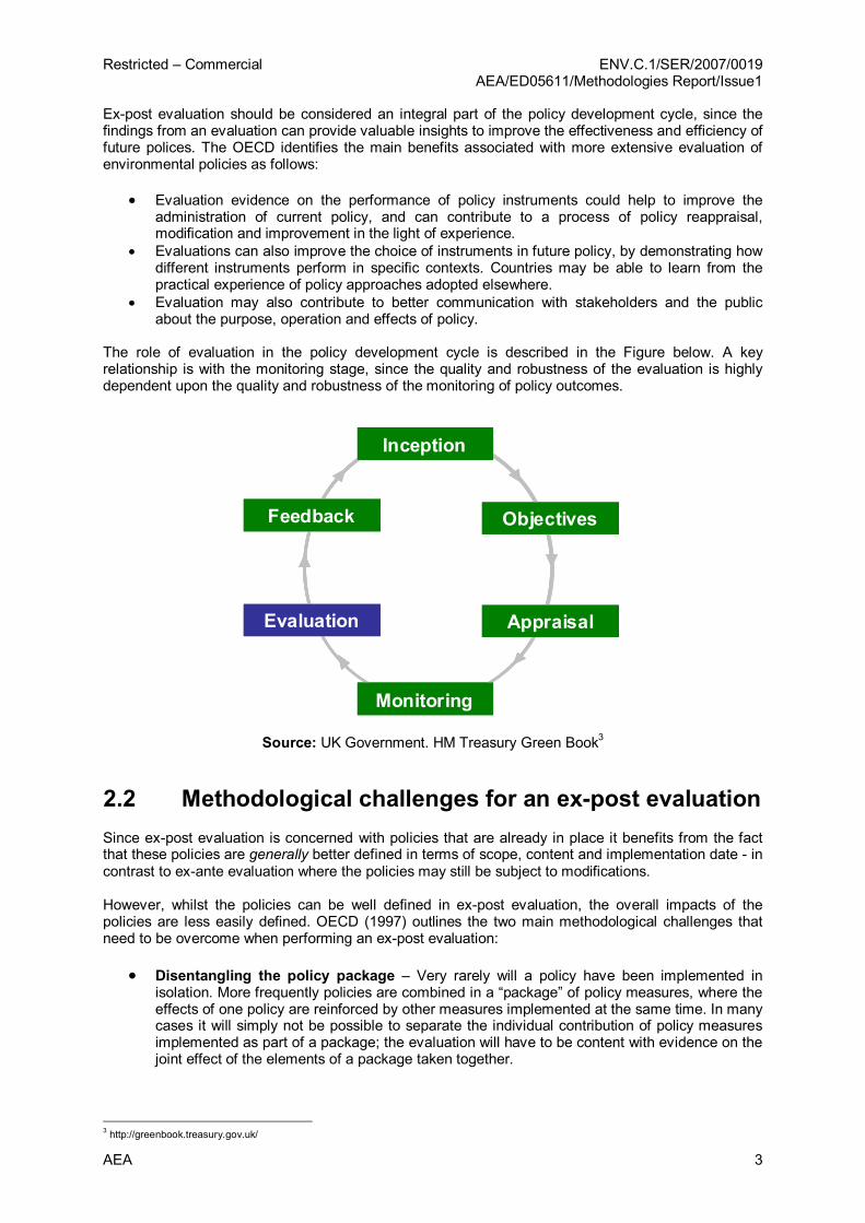
The role of evaluation in the policy development cycle is described in the Figure below. A key relationship is with the monitoring stage, since the quality and robustness of the evaluation is highly dependent upon the quality and robustness of the monitoring of policy outcomes.
Inception
Evaluation
Monitoring
Feedback
Appraisal
Objectives
Inception
Evaluation
Monitoring
Feedback
Appraisal
Objectives
Source: UK Government. HM Treasury Green Book 3
2.2 Methodological challenges for an expost evaluation Since expost evaluation is concerned with policies that are already in place it benefits from the fact that these policies are generally better defined in terms of scope, content and implementation date in contrast to exante evaluation where the policies may still be subject to modifications.
However, whilst the policies can be well defined in expost evaluation, the overall impacts of the policies are less easily defined. OECD (1997) outlines the two main methodological challenges that need to be overcome when performing an expost evaluation:
• Disentangling the policy package – Very rarely will a policy have been implemented in isolation. More frequently policies are combined in a “package” of policy measures, where the effects of one policy are reinforced by other measures implemented at the same time. In many cases it will simply not be possible to separate the individual contribution of policy measures implemented as part of a package; the evaluation will have to be content with evidence on the joint effect of the elements of a package taken together.
3 http://greenbook.treasury.gov.uk/
ENV.C.1/SER/2007/0019 Restricted – Commercial AEA/ED05611/Methodologies Report/Issue1
4 AEA
• Defining the counterfactual – It is unlikely that after the introduction of a policy or measure all effects on variables targeted by the policy in question (e.g. emissions of GHG, in the case of ECCP policies) can be attributed to the effects of that particular policy or measure. Some of the changes might have occurred anyway, regardless of whether the policy had been implemented or not. The effects of a policy change do not include all changes that took place subsequent to the policy change, but only those caused by the policy itself.
In addition to the above challenges, a further important issue that can significantly influence the consistency and comparability of results from different evaluations is:
• Defining the scope of the evaluation – This is particularly important where the evaluation is concerned with more than one policy, so consistency in the scope of the evaluation is important to enable a fair comparison of the results. Important considerations include the issue of policy ‘boundary’, for example the impacts of a policy may occur within the country in which the policy is implemented, but may have impacts outside of the country. Inclusion of the impacts that arise outside of the country can potentially lead to a very different outcome.
Associated with each of these general challenges are a series of more specific methodological issues that need to be taken into account when designing or performing an expost evaluation. In considering each of the issues, it is important to recognise that they may be related to the particular methodology that is used to in expost evaluation of the policy – since not all of the issues will be relevant to each of the evaluation methodologies. This is discussed further in Section 3.
Each of these challenges is discussed in more detail drawing upon examples from the published literature to illustrate the issue.
2.2.1 Disentangling the policy package
As described above, seldom does a policy impact upon a particular target in isolation. If these overlaps and synergies are not sufficiently resolved there is a danger that the individual policy evaluations will lead to double counting, where a certain proportion of the savings are claimed by both policies. This is particularly an issue where impacts are quantified using a ‘bottom up’ approach.
To help mitigate against the risk of double counting, evaluations should take explicit consideration of any policy overlaps and interactions. However, in some cases the policies are so intrinsically linked that it is difficult to disentangle the policy interactions. For example, TNO, IEEP and LAT (2006) reviewed various PAMs for reducing CO2 emissions from passenger cars. The review refers to four studies that aimed to evaluate the impact of the Labelling Directive (1999/94), but which found it impossible to disentangle the effect of this policy from the wider Voluntary Agreement policy package. Likewise, Joosen (2007) shows that the Dutch Energy Performance Standard have been deliberately designed to compliment some preexisting policies and interact with several other policies and measures.
These specific examples highlight the difficulty of disentangling policy impacts in some scenarios, especially where policies have been deliberately designed to compliment each other. This therefore justifies an evaluation of the ‘package’ of measures, where appropriate, in order to increase accuracy and reduce the risk of double counting.
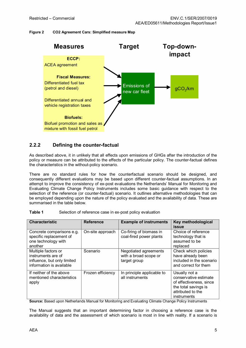
Under the OdysseeMure programme 4 a technique known as measures mapping has been developed to help understand and isolate the possible interactions/overlaps. The measures mapping approach works by screening the range of policies or measures that have an influence upon the same target or activity, and then mapping how the measures influence the available statistical data on the policy outcome. It is therefore useful for defining suitable activity indicators to evaluate polices, and to understand how policies impact upon the activities that are captured within emissions inventories (and therefore the potential for double counting). An example of a simplified measures map for the voluntary agreement (ACEA) for CO2 from passenger cars is shown below.
4 http://www.odysseeindicators.org/
Restricted – Commercial ENV.C.1/SER/2007/0019 AEA/ED05611/Methodologies Report/Issue1
AEA 5
Figure 2 CO2 Agreement Cars: Simplified measure Map
Target Topdown impact
Measures
Emissions of new car fleet gCO 2 /km
ECCP: ACEA agreement
Fiscal Measures: Differentiated fuel tax (petrol and diesel)
Differentiated annual and vehicle registration taxes
Biofuels: Biofuel promotion and sales as mixture with fossil fuel petrol
2.2.2 Defining the counterfactual
As described above, it in unlikely that all effects upon emissions of GHGs after the introduction of the policy or measure can be attributed to the effects of the particular policy. The counterfactual defines the characteristics in the withoutpolicy scenario.
There are no standard rules for how the counterfactual scenario should be designed, and consequently different evaluations may be based upon different counterfactual assumptions. In an attempt to improve the consistency of expost evaluations the Netherlands’ Manual for Monitoring and Evaluating Climate Change Policy Instruments includes some basic guidance with respect to the selection of the reference (or counterfactual) scenario. It outlines alternative methodologies that can be employed depending upon the nature of the policy evaluated and the availability of data. These are summarised in the table below.
Table 1 Selection of reference case in expost policy evaluation
Characteristic Reference Example of instruments Key methodological issue
Concrete comparisons e.g. specific replacement of one technology with another
Onsite approach Cofiring of biomass in coalfired power plants
Choice of reference technology that is assumed to be replaced
Multiple factors or instruments are of influence, but only limited information is available
Scenario Negotiated agreements with a broad scope or target group
Check which policies have already been included in the scenario and correct for them
If neither of the above mentioned characteristics apply
Frozen efficiency In principle applicable to all instruments
Usually not a conservative estimate of effectiveness, since the total savings is attributed to the instruments
Source: Based upon Netherlands Manual for Monitoring and Evaluating Climate Change Policy Instruments
The Manual suggests that an important determining factor in choosing a reference case is the availability of data and the assessment of which scenario is most in line with reality. If a scenario is

ENV.C.1/SER/2007/0019 Restricted – Commercial AEA/ED05611/Methodologies Report/Issue1
6 AEA
available, it may often be preferable to use it as the reference case. Linear extrapolation and frozen efficiency require limited data but are less accurate.
A specific issue that needs to be considered when defining the counterfactual is the influence of autonomous development. Autonomous development can potentially describe a range of inter related factors that influence the counterfactual trend in emissions, but are not captured within the scope of the evaluation. It may include, for example, the impact of autonomous technological improvement (i.e. innovation in technology). This is most applicable to policies that influence the take up of particular technologies. Autonomous policy development relates to the impact of policies implemented prior to the particular policy that is being evaluated (so is strongly related to how policy overlaps are dealt with in the evaluation). Finally, autonomous development is sometimes defined to reflect autonomous behaviour, where an activity would have occurred anyway, but has instead occurred in relation to a specific policy (see for example free riding described below).
Since autonomous developments can lead to GHG savings regardless of the introduction of the policy, then these savings should therefore be estimated and included in the counterfactual or subtracted from expost savings calculations to prevent overestimation of policy impacts. For example, certain improvements in the efficiency of boilers is likely to happen in the absence of any policy drivers, since improved efficiency represents a competitive advantage, so manufacturers have an incentive to deliver these improvements already. However, it can also be argued that the introduction of a policy can lead to a higher rate of improvement, or market transformation, which would not have occurred without the policy.
The isolation of the role of autonomous developments is complex, and often relies upon expert judgement. For example, it may be assumed that CO2 emissions from buildings will decrease over time in response to price signals (high energy costs). However, Joosen (2007) argues that property developers have no incentive to improve the energy performance of buildings as they are not responsible for paying the energy bills; improvements in performance from building design and construction are therefore more likely to be the result of policy obligations and should not be assumed to occur as autonomous savings.
Free riding (also known as deadweight) can occur where there is a prepolicy incentive to reduce emissions, e.g. a price signal to reduce energy consumption, which motivates consumers to invest in energy saving measures, then a policy that offers a further (positive) incentive to reduce emissions e.g. subsidisation of insulation, may result in a firm or household delaying action to reduce energy consumption until the implementation of the policy, or bringing forward action to take advantage of the incentive while it lasted. This would constitute freeriding.
To mitigate the risk of free riding it is possible to make an adjustment to the gross savings from the policy evaluation to take into account the estimated level of impact that would have occurred in the absence of the policy. This is the approach taken in the evaluation of the UK Energy Efficiency Commitment where an assessment is made of the number of installations, and the associated savings that would have occurred in the absence of the policy. This was determined on the basis of the pre policy ‘business as usual’ level of installations (Eion Lees Energy, 2006), and so required information on the status of the market prior to the implementation of the policy.
The Dutch Manual for monitoring and evaluating climate change policy instruments provides some basic guidance for determining the share of free rider activity, based on two possible routes. The first route involves making an assessment of whether the investment would have been made in the absence of a subsidy i.e. would it have been economically efficient to make the investment anyway. The second route is to undertake a survey the investor can be asked if he would have purchased the technology if no subsidy had been available. In both cases some additional analysis is required to determine the level of freeriding which may be extremely sector/policy specific.
Overall, the extent to which autonomous development or free rider behaviour is an issue, and can be corrected for, may vary considerably from policy to policy and from sector to sector. It may be possible, by examining statistical trends (e.g. linear extrapolation) prior to the implementation of the policy, to estimate the level of savings associated with autonomous developments. However, this is only applicable where the effects can be clearly defined and isolated.
Restricted – Commercial ENV.C.1/SER/2007/0019 AEA/ED05611/Methodologies Report/Issue1
AEA 7
A further issue that relates to the determination of the counterfactual scenario is the influence of hidden structural effects. Structural changes can be described in terms of the activity data that is used to estimate the emissions from the sector. Changes in the structure of this activity data may result in changes in the associated emissions, however, these structural changes may be effectively ‘hidden’ in the overall aggregate statistics – so the impacts of these changes are not isolated from the other factors driving emissions.
In some cases the structural effects can be identified and adjusted as part of the methodology e.g. closure of large industrial plant. However, other structural effects may be hidden, at least within the resolution of statistics made available to the evaluation. Expert review can be used to screen the data to identify anomalies and structural impacts on the emissions from the sector.
Once identified, hidden structural effects can be potentially correct for by making appropriate adjustments to the activity data to reflect the updated counterfactual scenario. However, correction for structural effects may require activity data to be made available, or collected, at a high level of granularity.
The rebound effect is an umbrella term for a number of mechanisms which reduce the size of the ‘energy savings’ achieved from improvements in energy efficiency. Direct rebound effects relate to individual energy services, such as heating and lighting, and are confined to the energy required to provide that service. Indirect rebound effects relate to the energy required to provide other goods and services, the consumption of which is affected by the energy efficiency improvement. The economy wide rebound effect represents the sum of direct and indirect rebound effects (Sorrell 2007 5 )
Rebound effects can be both direct (e.g. driving further in a fuelefficient car) and indirect (e.g. spending the money saved from more efficient heating on an overseas holiday). Direct rebound effects are related to the issues of defining the counterfactual, whereas indirect rebound effect are more related to how the scope of the evaluation is defined.
The UK Energy Research Centre performed an indepth review of rebound effects (UKERC, 2007). Reviewing over 500 papers and reports, the study analysed the nature, operation and importance of rebound effects and provided a comprehensive review of the available evidence on this topic, together with closely related issues, such as the link between energy consumption and economic growth. The evidence is that direct rebound effects are usually fairly small less than 30% for households for example. Much less is known about indirect effects. However the study suggests that in some cases, particularly where energy efficiency significantly decreases the cost of production of energy intensive goods, rebounds may be larger.
It is possible to capture direct rebound effects within the evaluation methodology, although the precise level of the rebound effect will be subject to debate, and may vary according to the socioeconomic characteristics of the affected population. Indirect rebound effects are best captured on an economy wide basis.
Certain factors with affect the savings both under the policy scenario (i.e. the policy may be more or less effective as a result of these factors) but also the counterfactual scenario. Correcting for these effects will determine the net impact of the policy, over and above the influence of these factors. This includes geographic/climatic factors, for example, the demand for heating services and the impacts of insulation measures on GHG impacts within different regions. Adjustments can be made with the evaluation methodology to ‘normalise’ these variations, and isolate the influence of these variables on the overall outcome.
There are a number of other exogenous factors, which may be exogenous to the policy evaluation, but can still have an influence upon the level of savings. The most significant factor is typically market prices. For example, energy prices will influence the demand for energy, and the associated CO2 emissions from industry, likewise, livestock numbers may be affected by meat and milk prices.
Where it is not possible to capture these factors within the methodology a high level assessment of the potential impacts could be carried out by means of a sensitivity analysis e.g. if the price elasticity of demand for energy was set at a certain level then how would this change the overall result.
5 UKERC Review of Evidence for the Rebound Effect. Supplementary Note: Graphical illustrations of rebound effects. Working Paper October 2007: REF UKERC/WP/TPA/2007/014. Steve Sorrell Sussex Energy Group (SEG) University of Sussex
ENV.C.1/SER/2007/0019 Restricted – Commercial AEA/ED05611/Methodologies Report/Issue1
8 AEA
2.2.3 Defining the scope of the evaluation
A number of factors relating to how the scope of the evaluation is defined can influence the overall results that are achieved and the overall comparability of results.
An announcement effect can be defined in terms of an action taken to reduce emissions as a result of a policy, between the time of the announcement of the policy and its implementation, when this action would not have been taken if the policy had not been announced. Likewise a delay effect, relates the fact that whilst a policy may have officially begun on a certain data, the measures implemented as a results of the policy may have been delayed.
From an evaluation perspective this relates to how the policy is defined, specifically its start date. Joosen (2007), for example, describes how the Dutch Energy Performance Standards were prepared over an extended period of time and through consultation with industry. This gradual process of design, and the deliberate forewarning of industry as to the targets they will be expected to meet, means that it is hard to delineate the period before and after which industry began reacting to the presence of the policy (i.e. its impact).
The identification of announcement or delay effects is typically a judgement call so requires a detailed understanding of the policy development and subsequent implementation. Announcement or delay effects are typically dealt with by extending the scope of the evaluation to the date of the policy announcement, or reduce it to reflect any delays.
Another issue that relates to the scope of the evaluation, but also to the methodology that is employed is multiplier effects. Multiplier effects (also known as spill over effects) occur where the implementation of the policies leads to wider impacts beyond the boundary of the policy evaluation. For example, Ellerman (2003) cites evidence of an innovation effect from emissions trading policies in the case of SO2 in the US. In this instance the trading scheme brought about environmental impacts that are not directly associated with the policy instrument, but which will help the policy to achieve its objectives.
Joosen (2007) shows that the Dutch Energy Performance Standard has led to substantial spill over effects in the market for consumer products. The standard has contributed to the growth of market share of condensing boilers and high performance glazing to such an extent that these have now become standard techniques within the market place, leading to additional GHG savings beyond the direct impact of the policy. Likewise, the evaluation of the UK’s Energy Efficiency Commitment (EEC) by Eion Lees Energy (2006) concluded that the financial support provided under EEC, along with other policy initiatives, has successfully transformed the cold and wet appliance market much more rapidly than might have been expected from historical trends.
The main challenge for evaluating multiplier effects is providing a quantitative assessment of the GHG impacts in the absence of empirical data. For specific policies, and specific markets, data may be available to enable a quantitative assessment of the market transformation effects. However, in most evaluations multiplier effects can only be assessed in qualitative terms.
The consideration of multiplier effects also relates to the approach that is used to evaluate the impacts. Bottom up methods may underestimate multiplier effects if they occur outside of the target group. In contrast topdown methods may already include multiplier effects in the estimated savings, but may struggle to isolate them.
Other spillover effects can have an important impact on the overall outcome, especially when the influence of the spillover effects is greater than the direct effects. For example, the displacement of emissions causing activities to another global location may reduce the net emissions in one country, but lead to greater emissions within another country. At a global level the net impacts may be highly uncertain and difficult to quantify, but may in some cases lead to net increase in emissions. For example, if the displaced activity is less efficient or leads to significant carbon impacts from land use change.
Restricted – Commercial ENV.C.1/SER/2007/0019 AEA/ED05611/Methodologies Report/Issue1
AEA 9
A related issue is indirect rebound effects. As described above these are typically difficult to quantify at an individual policy level, and are best dealt with at an aggregate level using macroeconomic models.
2.3 Type of methodologies A variety of methods are available for application in the expost evaluation of the impact of policy instruments. These can be broadly categorised into two main types of approach:
Ø Topdown evaluation refers to methods relying on statistical indicators defined by sector and/or type of enduse from national/macrolevel data in order to evaluate the impacts of a measure or policy.
Ø Bottomup methods start from data at the level of a single emissions reduction measure, mechanism, programme, or service and then aggregates results from all measures reported by a Member State to assess its total emissions savings in a specific field. This allows more detailed modelling of the impacts of policies and measures by parameterising the measure impacts, i.e. by determining what kind of technology or behaviour is influenced by the measure and in which way.
In reality, however, the spectrum of methods is much broader depending on the degree of detail available for the data. Nilsson et al (2007), summarising the results from the EMEEES 6 project identified 9 separate methodologies, which fall into four separate types two topdown and two bottomup approaches. These are described in turn below.
2.3.1 Simple topdown approach based on indicators
In this approach the policies are evaluated using aggregated statistics for the relevant sectors considered. A hypothetical counterfactual scenario is constructed assuming the level of greenhouse gas emissions either stays unchanged from the base year or is adjusted for autonomous developments. The actual greenhouse gas emissions are then subtracted from this amount and the difference is defined as the impact of a policy instrument or a package of policy instruments.
The major advantage of this methodology is that it requires only a relatively high level statistical data set to derive an initial estimate of the overall policy impacts. This is likely to require minimal additional data collection, relying instead upon established datasets. It can be applied consistently across a range of Member States and sectors, and does not necessarily require a large amount of computational effort. Where more disaggregated data is available the methodology can be refined to provide a more accurate assessment of the policy impacts at a subsectoral level, and to take more explicit consideration of the socioeconomics drivers of emissions.
The major disadvantage of these types of models is that they typically have a rather limited representation of the sectors considered and do not fully incorporate technological options to reduce GHG emissions. Likewise, structural effects and social developments (e.g. increased demand for energy service) are typically not isolated from the policy impacts. Therefore, since this methodology typically takes a simplistic counterfactual, and assumes the total difference between the counter factual and the actual emissions can be attributed to the policy, then the projected savings are likely to represents an upper estimate of the actual impact.
Furthermore, unless ‘autonomous’ savings are explicitly accounted for this method does not provide any insight as to the actual effect of policies as the calculated amount of GHG saving is the aggregation of autonomous and policy induced savings. A related issue is that even when autonomous savings are taken into account the residual ‘policy impact’ may include several measures, making it extremely difficult to isolate individual policy impacts.
6 http://www.evaluateenergysavings.eu/emeees/en/home/index.php
ENV.C.1/SER/2007/0019 Restricted – Commercial AEA/ED05611/Methodologies Report/Issue1
10 AEA
2.3.2 Refined top down approach
Like the sectoral indicators based method described above, a refined top down approach also relies upon aggregate statistics, but examines in more detail the relationship between the key parameters and the GHG emissions in order to disentangle the impact of the policy instrument. In the modelling, a list of factors (one of which is the analysed policy instrument) is drawn up that potentially could affect (specific) greenhouse gas emissions per sector or country. Through statistical methods, the impact of the analysed policy instruments can be estimated. For this purpose secondary statistics and statistical analysis are integrated into the approach.
As refined topdown approaches typically draw upon a more comprehensive body of statistical data they are both more data and time intensive than the indicators based methods. However, in the refined approach the counterfactual scenario is based more upon an understanding of the key socio economic drivers of greenhouse gas emissions, and attempts to disentangle the effects for the policy impacts. It is therefore much less likely to overestimate the policy impacts than in the simple topdown approach.
Refined statistical models have the further advantage that they can provide consistent scenarios in terms of GDP, labour productivity, consumption and investment expenditure, government balances, etc across all sectors and regions analysed. They are also better suited to analyse indirect costs such as effects on GDP, welfare loss, and employment impacts.
However, like the indicators based methodology the refined top down approach has the potential to include a number of exogenous effects, which are not necessarily due to the impact of the policies, including price induced effects or autonomous technical progress. A further limitation is that the method does not provide insight into ‘why’ an instrument had an impact or not.
2.3.3 Bottom up methods
The most detailed approach consists of a bottomup data collection and analysis of GHG savings, where the data collection may rely either on direct measurements or on expert estimates with or without site visits.
Bottomup policy evaluations tend to focus on determining the ‘final effects’ of a single policy instrument or a package of instruments. These evaluation methods typically use data at the level of a single policy measure, mechanism or programme and then aggregate results from all measures reported by a Member State to assess the total GHG emission savings.
The scope of bottomup models is typically much narrower than for topdown assessments. Usually, bottomup models do not deal with the whole economy, but only with some particular aspects that are modelled in great detail, such as: the whole emission system, the energy system, the transport system. Bottom up methods are typically driven by engineering estimates and technological choices. The required data can be obtained by either direct measurement or expert estimates.
A number of variations on bottom up methodologies are available, and typically reflect the amount and type of information that is available. Nilsson et al (2007) provides a review of 26 case studies in the area of energy efficiency policy evaluation for the EMEEES project. The bottom up evaluation methods are categorised into a number of subgroups, as follows:
• Direct measurement of energy savings with the subject of the evaluation being a participant in a energy efficiency measure;
• Energy bills & sales data analysis to determine energy savings with the subject of evaluation being a participant. Billing analysis can be based upon sample or all participants;
• Enhanced engineering estimates can involve a mix of audit results, energy modelling, and expost measurements having either a participant or a certain type of measure or technology as the subject of the evaluation;
• Mixed deemed and expost evaluation concerns the energy savings from a certain type of measure or technology and can be based upon equipment sales data, measurements, samples etc. It is not considered to be as exact as engineering estimates;

Restricted – Commercial ENV.C.1/SER/2007/0019 AEA/ED05611/Methodologies Report/Issue1
AEA 11
• Deemed estimates quantify the energy saving from a certain type of measure or technology and ascribes the same amount of energy saving to each unit for a specific type of measure;
• Bottom up modelling based on surveys of population samples is modelling the whole stock of buildings or equipment or modelling the whole energy consumption for an enduse or sector. The surveys are needed to identify which enduse energy efficiency actions have been taken and why.
The major advantage of bottomup evaluation methods is the fact that they can allow a direct monitoring of the savings that are due to the particular policy. This approach can thus, theoretically, achieve a greater level of accuracy. In practice, however, "Freeridereffects" and the uncertainties associated with defining the counterfactual can have a large impact upon the precision of the method.
The main drawback of bottomup evaluations, however, is the potentially high costs of data collection, if a high level of accuracy is deemed necessary. Although the collection of monitoring data may have additional benefits beyond the policy evaluation such as the development of benchmarks and a better programme design.
A further limitation of bottomup models is that they are not usually able to consider feedback effects on the wider economy (apart from price elasticities). Likewise bottom up methods may not adequately address overlaps between measures and face the risk of double counting the savings.
2.3.4 Combined top down/bottom up approach
Both bottom up and top down evaluation methods have certain advantages and drawbacks, i.e. there is a tradeoff between accuracy and the costs of evaluation. Combining topdown and bottomup evaluation in an integrated method allows for crosschecking of the results, and can potentially lead to higher accuracy and/or lower costs.
Integrated methods combine top down sector statistics with policy specific bottom up data. Like the other methods the complexity and data requirements of integrated methods can vary widely. One application of an integrated method is to use top down statistics to provide a first estimate of the potential impacts of policies within a sector (e.g. applying an indicators based approach) and then supporting this with a more detailed bottom up analysis of the main policies within the sector. Another variant is to allow, depending on the sector and on the data availability, for a flexible application of the methods. For example, this might mean that certain policies are evaluated predominantly based upon topdown data, and other policies/sector might be assessed using bottom up data – all within the same integrated framework.
Integrated methods have the benefits of combining the simplicity of the top down methods with the rigour of the bottom up methods. The major advantage is the higher precision over a standalone top down approach with a still relatively reasonable additional cost for the evaluation.
However, a key challenge for these methods is linking the two data sets and dealing with discrepancies. The successful application of an integrated approach therefore requires the acceptance of the data and of the methods by all stakeholders.
2.3.5 Comparison of the methods
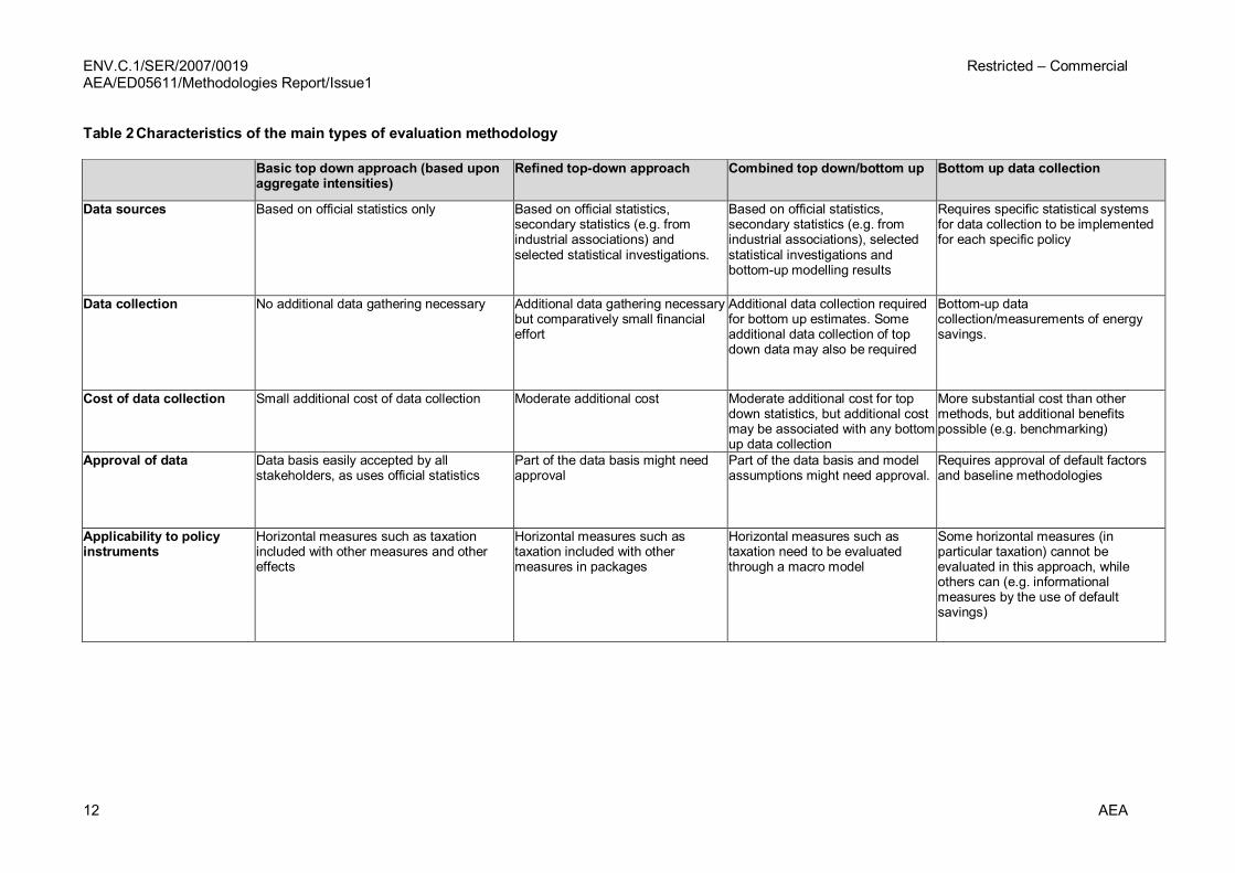
The following table provides a comparison of the main characteristics of the different methods. The summary is based upon the generic characteristics of the different methods.
ENV.C.1/SER/2007/0019 Restricted – Commercial AEA/ED05611/Methodologies Report/Issue1
12 AEA
Table 2Characteristics of the main types of evaluation methodology
Basic top down approach (based upon aggregate intensities)
Refined topdown approach Combined top down/bottom up Bottom up data collection
Data sources Based on official statistics only Based on official statistics, secondary statistics (e.g. from industrial associations) and selected statistical investigations.
Based on official statistics, secondary statistics (e.g. from industrial associations), selected statistical investigations and bottomup modelling results
Requires specific statistical systems for data collection to be implemented for each specific policy
Data collection No additional data gathering necessary Additional data gathering necessary but comparatively small financial effort
Additional data collection required for bottom up estimates. Some additional data collection of top down data may also be required
Bottomup data collection/measurements of energy savings.
Cost of data collection Small additional cost of data collection Moderate additional cost Moderate additional cost for top down statistics, but additional cost may be associated with any bottom up data collection
More substantial cost than other methods, but additional benefits possible (e.g. benchmarking)
Approval of data Data basis easily accepted by all stakeholders, as uses official statistics
Part of the data basis might need approval
Part of the data basis and model assumptions might need approval.
Requires approval of default factors and baseline methodologies
Applicability to policy instruments
Horizontal measures such as taxation included with other measures and other effects
Horizontal measures such as taxation included with other measures in packages
Horizontal measures such as taxation need to be evaluated through a macro model
Some horizontal measures (in particular taxation) cannot be evaluated in this approach, while others can (e.g. informational measures by the use of default savings)

Restricted – Commercial ENV.C.1/SER/2007/0019 AEA/ED05611/Methodologies Report/Issue1
AEA 13
Basic top down approach (based upon aggregate intensities)
Refined topdown approach Combined top down/bottom up Bottom up data collection
Isolation of policy impacts The savings estimate may contain other exogenous factors in addition to the impacts of the policy (see below)
The savings estimate may contain other exogenous factors in addition to the impacts of the policy (see below)
All important factors of influence are established separately
The savings estimate may contain other exogenous factors in addition to the impacts of the policy (see below)
Policy impacts Savings estimate will include policy impacts that are not part of the policy under consideration (e.g. some horizontal measures, possibly standalone training information measure).
Savings estimate may include some policy impacts that are not part of the policy under consideration, and could not be isolated.
All important policy impacts are shown individually in their contribution, i.e. separate from the policy impacts.
Savings estimate may include some policy impacts which are not part of the policy under consideration (through double counting of energy saving measures if they are not properly associated to a particular programme).
Autonomous technical changes
Autonomous technical changes are not isolated from the policy impacts
Autonomous technical changes are isolated based on (econometric) estimates
Autonomous technical changes are isolated based on (econometric) estimates
Autonomous technical changes (not policy induced) may not be captured
Structural changes Does not isolate structural changes in the economy, e.g. Tertiarisation of the economy shift from heavier to lighter industries structural changes within industrial branches and within companies
Does not isolate some smaller remains of structural changes in the economy, e.g. structural changes within industrial branches and within companies
All important contributions to structural changes are shown separately from the policy impacts
Structural changes in the economy, are completely eliminated in this approach
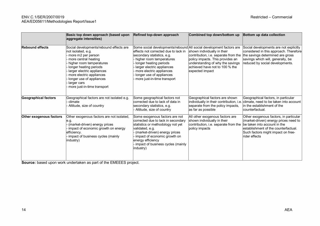
ENV.C.1/SER/2007/0019 Restricted – Commercial AEA/ED05611/Methodologies Report/Issue1
14 AEA
Basic top down approach (based upon aggregate intensities)
Refined topdown approach Combined top down/bottom up Bottom up data collection
Rebound effects Social developments/rebound effects are not isolated, e.g. more m2 per person more central heating higher room temperatures longer heating periods larger electric appliances more electric appliances longer use of appliances larger cars more justintime transport
Some social developments/rebound effects not corrected due to lack in secondary statistics, e.g. higher room temperatures longer heating periods larger electric appliances more electric appliances longer use of appliances more justintime transport
All social development factors are shown individually in their contribution, i.e. separate from the policy impacts. This provides an understanding of why the savings achieved have not to 100 % the expected impact
Social developments are not explicitly considered in this approach. Therefore the savings determined are gross savings which will, generally, be reduced by social developments.
Geographical factors Geographical factors are not isolated e.g. climate Altitude, size of country
Some geographical factors not corrected due to lack of data in secondary statistics, e.g. Altitude, size of country
Geographical factors are shown individually in their contribution, i.e. separate from the policy impacts, as far as possible
Geographical factors, in particular climate, need to be taken into account in the establishment of the counterfactual.
Other exogenous factors Other exogenous factors are not isolated, e.g. (marketdriven) energy prices impact of economic growth on energy efficiency. impact of business cycles (mainly industry)
Some exogenous factors are not corrected due to lack in secondary statistics or methodology not yet validated, e.g. (marketdriven) energy prices impact of economic growth on energy efficiency impact of business cycles (mainly industry)
All other exogenous factors are shown individually in their contribution, i.e. separate from the policy impacts
Other exogenous factors, in particular (marketdriven) energy prices need to be taken into account in the establishment of the counterfactual. Such factors might impact on free rider effects
Source: based upon work undertaken as part of the EMEEES project.

Restricted – Commercial ENV.C.1/SER/2007/0019 AEA/ED05611/Methodologies Report/Issue1
AEA 15
2.3.6 Methodological issues associated with each of the approaches
As described above there are a range of methodological issues that need to be considered when performing an expost evaluation. These issues will vary according to the type of methodology that is being employed. Topdown and Bottomup approaches are both influenced by a different set of effects, which can make the evaluation of the GHGsaving impact difficult.
Topdown approaches suffer from the following effects:
• Rebound effects might not be completely separated from the savings (e. g. increased internal temperatures in houses at the end of the measure evaluation period as compared to the beginning of the period, e.g. due to general lifestyle changes and increase in welfare). They tend to diminish the observed gross savings.
• Autonomous savings and ongoing savings from previous policy measures will give rise to an overestimate of savings, if observed gross savings are taken as the measure of real savings.
• Structural effects that are not sufficiently resolved (i.e. hidden) can increase or decrease the savings.
• Exogenous factors such as market energy prices change the conditions for autonomous savings. When energy prices increase, autonomous savings tend to increase and economic rebound effects to decrease (but the latter only very slowly).
Bottomup approaches are more likely to suffer from the following effects:
• Direct rebound effects (e.g. increased internal temperatures in houses due to energy efficiency improvements allowing higher indoor temperatures at moderate costs) give rise to an overestimate of the real savings achieved
• Free riders may also be a problem for bottom up evaluations of grants and subsidy schemes.
• Difficulties with the quantification of multiplier effects may lead to an underestimate of the net savings.
• Policy overlaps (where several measures have positive or negative synergies when implemented in conjunction) may not be adequately addressed within the methodology. The net effect can lead to either an overestimation or an underestimation of the savings, depending upon the nature of the synergies.
• Exogenous factors such as market energy prices will change the conditions for free riders, direct rebound effects, multiplier effects and measure interactions.
When topdown and bottomup methods are used in parallel to evaluate the same measure as part of a combined approach, the challenge is to make clear how topdown and bottomup methods match in terms of the definitions and calculation methods. This needs to take into account the various methodological issues described above. The figure below illustrates how the estimates of savings from topdown and bottom up methods compare.
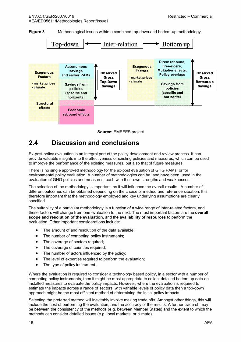
ENV.C.1/SER/2007/0019 Restricted – Commercial AEA/ED05611/Methodologies Report/Issue1
16 AEA
Figure 3 Methodological issues within a combined topdown and bottomup methodology
Direct rebound, Freeriders,
Multiplier effects, Policy overlaps
Economic rebound effects
Observed Gross
TopDown Savings
Exogenous Factors
market prices climate
Topdown Bottom up
Structural effects
Observed Gross
Bottomup Savings
Interrelation
Autonomous savings
and earlier PAMs
Savings from policies
(specific and horizontal
Savings from policies
(specific and horizontal
Exogenous Factors
market prices climate
Source: EMEEES project
2.4 Discussion and conclusions Expost policy evaluation is an integral part of the policy development and review process. It can provide valuable insights into the effectiveness of existing policies and measures, which can be used to improve the performance of the existing measures, but also that of future measures.
There is no single approved methodology for the expost evaluation of GHG PAMs, or for environmental policy evaluation. A number of methodologies can be, and have been, used in the evaluation of GHG policies and measures, each with their own strengths and weaknesses.
The selection of the methodology is important, as it will influence the overall results. A number of different outcomes can be obtained depending on the choice of method and reference situation. It is therefore important that the methodology employed and key underlying assumptions are clearly specified.
The suitability of a particular methodology is a function of a wide range of interrelated factors, and these factors will change from one evaluation to the next. The most important factors are the overall scope and resolution of the evaluation, and the availability of resources to perform the evaluation. Other important considerations include:
• The amount of and resolution of the data available; • The number of competing policy instruments; • The coverage of sectors required; • The coverage of counties required; • The number of actors influenced by the policy; • The level of expertise required to perform the evaluation; • The type of policy instrument.
Where the evaluation is required to consider a technology based policy, in a sector with a number of competing policy instruments, then it might be most appropriate to collect detailed bottom up data on installed measures to evaluate the policy impacts. However, where the evaluation is required to estimate the impacts across a range of sectors, with variable levels of policy data then a topdown approach might be the most efficient method of determining the initial policy impacts.
Selecting the preferred method will inevitably involve making trade offs. Amongst other things, this will include the cost of performing the evaluation, and the accuracy of the results. A further trade off may be between the consistency of the methods (e.g. between Member States) and the extent to which the methods can consider detailed issues (e.g. local markets, or climate).
Restricted – Commercial ENV.C.1/SER/2007/0019 AEA/ED05611/Methodologies Report/Issue1
AEA 17
3 Proposed methodological approach for the expost evaluation of EU Climate Change Policies
This section focuses on the methodological framework for the expost quantification of the impact of EU policies and measures from the ECCP, for individual Member States and for the EU27 as a whole.
In the case of policies and measures implemented as part of the ECCP the primary impact of concern is the reduction in greenhouse gas emissions 7 . Quantifying the policy impacts requires an assessment of the GHG emissions with the policy in place, as well as an assessment of the GHG emissions if the ECCP policies were not implemented i.e. the emissions under the counterfactual scenario (also known as the reference scenario).
Under the UNFCCC (United Nations Framework Convention on Climate Change) participating nations are required to implement an emissions inventory that records historical emissions of greenhouse gases. Therefore, statistical information is available on the overall historical changes in GHG emissions that have occurred over the period during which the ECCP PAMs have been implemented. In addition, Member States may have in place some monitoring and tracking systems related to specific policies, such as information on the number and capacity of renewable energy devices installed. These statistics can also be used to underpin the analysis of the ECCP policy impacts.
A key challenge for this study has been the fact that the methodologies are reliant upon existing data. So whilst the analysis has identified existing data needs to improve future evaluations, the current methods are largely based upon existing data sets. Therefore, where the existing monitoring of policies is limited, or not sufficiently focussed on GHG emissions then the overall evaluation methodologies will be more uncertain.
As highlighted in section 2 different evaluation approaches may be appropriate, depending on the goals of the evaluation, data availability, characteristics of a policy, capabilities of the evaluators and so on.
The first step in defining a methodology for the evaluation of the EU Climate Change Policies is therefore to define criteria to help identify the approach that best responds to requirements of the relevant stakeholders involved in ECCP evaluation. This step is illustrated in section 3.1 below.
On the basis of this step, a general framework can be developed for guidelines to evaluate EU Climate change policies (section 3.3) and choices can be made on key approaches and issues concerning the articulation and use of policy evaluation guidelines (see chapter 4).
3.1 Selecting a methodological framework In selecting the methodological framework consideration has been given to the relative strengths and weaknesses of the methodologies with the objective of identifying the most suitable approach for application in this study.
As described in Section 2 there is a range of potential methodologies that are available for expost policy evaluation. It is not possible to assess each of the many different methodologies individually given the breadth of their scope and coverage. Therefore, to enable a meaningful evaluation of the methodologies we have taken the broad classification of methodologies described previously.
Specifically the methodologies have been evaluated according to the following classification: • Basic top down approach (based upon aggregate intensities) • Refined topdown approach • Combined top down/bottom up (also known as integrated methods) • Bottom up data collection
7 Although it should be noted that certain policies within the ECCP have been primarily designed to meet other policy objectives and GHG emissions reduction is a secondary (although still potentially substantial) benefit, examples include the Large Combustion Plant Directive, the IPPC Directive and the Common Agricultural Policy.
ENV.C.1/SER/2007/0019 Restricted – Commercial AEA/ED05611/Methodologies Report/Issue1
18 AEA
A series of criteria were drawn up to evaluate the above methodologies, the definitions for which and the evaluation results are presented in the following sections. Note this criteria may not necessarily reflect the requirements of other evaluations where the scope may be narrower i.e. focused on just one policy of measure, or where wider consideration are included in the scope of the evaluation.
3.1.1 Applicability
Criteria: The methodology or methodologies should be applicable to the ex post evaluation of different policy instruments, different sectors and across all Member States.
• Basic and Refined topdown approach
These methods have been widely used to assess policy impacts across a range of sectors and countries, although the focus to date has largely been upon the energy sector. They have also been used to assess specific policies or measures. However, the level of disaggregation means that the methods are better suited to the evaluation of packages of policies and measures than individual policy instruments. They may, therefore, be less suited to sectors where there are a large number of interacting policies e.g. energy demand in the residential sector, unless they can be combined with bottom up data or secondary statistics
Top down approaches are applicable to most types of policy instruments, although they are less applicable where a degree of technological disaggregation is required. For evaluating instruments with price effects then econometric models are required.
• Bottomup data collection
Methodologies have been developed to assess a range of policies and sectors. Frequently, the approaches have been developed as bespoke models so may not be fully consistent across sectors or between Member States. The meaningful application of these methodologies to a range of sectors may, therefore, require agreement of the underlying assumptions and saving factors.
Bottom up methods can be tailored to most types of policy instrument, but are best suited to technologyfocussed measures. They are less appropriate for some horizontal policy instruments (in particular tax measured), although they can be adapted for others (e.g. informational measures by the use of default savings).
• Combined top down/bottom up
Combined top down/bottom up approaches can in theory take on the characteristics of both the top down and bottom up methods, so are applicable to all sectors and policy instruments. This may involve certain measures being quantified predominantly using topdown statistics, but for others the impacts may be evaluated using bottom up data. Where existing methodologies exist (e.g. for bottom up assessment of energy efficiency measures) then further work may be required to ensure that the combined methodology is consistent in its approach.
3.1.2 Consistency
Criteria: The methods should make use of existing national and international data sources and data collection frameworks. In particular, the methods should be consistent with National Inventories and Registries. It will also be important to take into account any ongoing or proposed data collection activities e.g. the requirements of the Energy Services Directive
• Basic/Refined topdown approach
The top down nature of these methods usually mean that they are underpinned by national statistics such as the data reported in national emission inventories. This is a clear advantage of using a top down approach to policy evaluation.

Restricted – Commercial ENV.C.1/SER/2007/0019 AEA/ED05611/Methodologies Report/Issue1
AEA 19
However, whilst the data will be consistent with national statistics it may be less consistent with the sector or sub sector level activity data depending upon the level of complexity of the model and the degree of calibration. This may lead to inconsistencies where policies are monitored at a more disaggregated level.
Where secondary statistics are used as part of a refined approach then this may lead to some inconsistency where different data sets may be required for different sectors and /or Member States.
• Bottomup data collection
Since bottom up methods are typical built upon survey data, which is then scaled up, then the methods are usually less consistent with the aggregate statistics. This may require the use of correction factors.
• Combined top down/bottom up
Consistency checking is an integral component of combined methods, since they are required to integrate aggregate statistics with bottom up data. Whilst this creates initial challenges, and additional resource requirements, it ensures that the estimates are most consistent with both national inventories, and also bottom up statistics.
3.1.3 Transparency
Criteria: The methods should be transparent and simple, i.e. policy makers should be able to workout for themselves how the impacts are determined. This will include a clear disaggregation of the policy impacts upon emission, from the impacts of other socioeconomic variables.
• Basic topdown approach
These methods can vary in complexity and thus transparency. Where the reference case has been defined on the basis of simplistic assumptions e.g. frozen efficiency, then the analytical basis is relatively transparent. However, as the modelling become more complex the transparency of the methodology can become less clear. A decomposition based approach can be useful in providing transparent outputs of the key drivers of emissions changes.
• Refined topdown approach
Econometric models by their very nature will be more complex than the indicators based approach. Whilst the econometric relationships can be made transparent, models of this kind typically suffer poorer transparency unless the trends and interrelationships can be clearly described.
• Bottomup data collection
The transparency of these methods relates closely to the level of complexity of the methods – and the complexity can vary greatly between one methodology and the next. Where the input data is clearly identified and the modelling parameters clearly specified the outputs are reasonably transparent. However, where the modelling becomes more complex, for example, to take into account rebound effects and correction factors, the transparency can be reduced.
• Combined top down/bottom up
Transparency may be a problem for combined methods as they integrate a range of different types of data
ENV.C.1/SER/2007/0019 Restricted – Commercial AEA/ED05611/Methodologies Report/Issue1
20 AEA
3.1.4 Robustness
Criteria: The methods should be based upon robust principles, with uncertainties clearly identified and a far as possible quantified.
• Basic topdown approach
Since these methods typically take a more simplistic view of the policy impacts the outputs are typically less robust than for some of the other methods when assessing individual policy impacts. Sensitivity analysis can be relatively easily applied to the basic assumptions to give an indication of the influence of the main deterministic parameters on the estimate.
• Refined topdown approach
Econometric models are based upon longrun statistical relationships. This provides greater confidence in the policy impacts and enables sensitivity analysis to be based upon statistical relationships. However, where secondary statistics are limited, or incomplete, then this will impact upon the robustness of the method.
• Bottomup data collection
Whilst these methods are typical based upon more extensive data sets and detailed information, the robustness of the methods will reflect the quality of the underlying data sets and modelling assumptions. For example, if the analysis is based upon survey data then the robustness with relate to how representative the survey data is.
• Combined top down/bottom up
By combining separate estimates, based upon both top down statistics and bottom up data combined methods include a degree of selfvalidation. However, where the bottom and top down estimates cannot be calibrated then the results may be perceived as a less robust than where a single result is presented.
3.1.5 Policy relevant
Criteria: The methods should be able to explain the impact of climate change policies on the national and/or sectoral level. It will also be important to understand the impact of ECCP PAMs as opposed to other national policies
• Basic/refined topdown approach
It may be difficult to disaggregate the impacts of individual policies and measures using topdown methods. These methods do not typically describe the complexity of the individual sectors very well, which can make it difficult to unpick the influence of individual polices where the policy framework is complex.
A fined approach can improve the resolution of the analysis and therefore the ability to identify the influence of specific policies. Certain horizontal measures (e.g. taxes) can only really be addressed adequately through an econometric approach.
• Bottomup data collection
Bottom up methods typically draw upon policy specific activity data so are typically much more able to describe individual policy impacts. However, where several policies are impacting upon the same sector it may still be difficult to adjust for policy overlaps.
Restricted – Commercial ENV.C.1/SER/2007/0019 AEA/ED05611/Methodologies Report/Issue1
AEA 21
Bottom up methods may not be appropriate for evaluating certain horizontal instruments – specifically taxes.
3.1.6 Complexity
Criteria: The methods should be sufficiently developed to ensure a robust quantification of the GHG impacts. The methods should not require a large amount of new data or expertise.
• Basic topdown approach
Indicator based methods are typically rather simplistic in their approach are therefore relatively easy to implement. An additional advantage of these methods is they require limited additional data collection. More complex applications of the methodology are also possible which may require additional data and expertise.
• Refined topdown approach
Econometric methods require a higher level of expertise than indicators based approach. They require a more extensive data set, which may require secondary statistics.
• Bottomup data collection
Methods are extremely variable in the complexity and depend upon the amount of policy monitoring data that is available. The methods are typically developed at a sectoral level by sector experts.
• Combined top down/bottom up
Combined methods have the potentially to be extremely complex, since they incorporate both top down statistics and bottom up data. However, the methods can be developed in a flexible way to accommodate the data that is available. For example, for certain sectors the methods may assess policies predominantly using top down data e.g. energy supply sector), however, for other sector (e.g. residential sector) the approach may draw upon much more bottom up data – so the complexity of the method would increase.
3.1.7 Flexibility
Criteria: The methods should be sufficient flexible to deal with variable data quality and also be able to be adjusted to reflect updated assumptions.
• Basic topdown approach
Since indicator based methods are based upon top down indicators then they are typically able to be applied to a range of sectors.
• Refined topdown approach
The methods have a high data requirement to inform the econometric relationships. If this data is not available then may require considerable time and effort to modify the approach
• Bottomup data collection
These methods are typically extremely flexible as they are developed on a bespoke basis to reflect the level of data that is available. However, where a standardised approach and method is required then this approach might be less flexible.
• Combined top down/bottom up

ENV.C.1/SER/2007/0019 Restricted – Commercial AEA/ED05611/Methodologies Report/Issue1
22 AEA
Combined methods are potentially most flexible as they can accommodate estimates from both top down and bottom up data.
3.2 Overall evaluation of methodologies Building upon the review of the strengths and weaknesses of the respective methodologies described above, it can be concluded that an integrated approach (combining elements of both topdown and bottom up methods) is the most appropriate single methodology for the expost evaluation of the EU climate change policies.
However, there is recognition that resource constraints and data availability are an important consideration for the development of a methodology for expost policy evaluation. Methods may become increasingly complex and resource intensive with diminishing returns to the quality of estimates. Different Member States may have access to different data sets, and data availability may vary significantly either within a Member State or between climate change policies. This demands solutions that maintain some adaptability and can meet various requirements.
As part of this project discussion of an appropriate methodological framework was undertaken with key Member State stakeholders at a workshop that took place in Brussels on February 26, 2008. This again highlighted the tradeoffs between the desire for a robust integrated approach, as highlighted by the evaluation, and some of the direct practical constraints that exist.
The outcome of this was the decision to pursue a tiered approach to evaluation of EU Climate Change Policies 8 . The framework starts with the most straightforward, but potentially less robust, topdown methods (which may be the only approach possible, e.g. given issues of data availability) and then moves up tiers of increasing complexity, towards the preferred, integrated, approach. The methodological framework is discussed in more detail in the following section.
3.3 The methodological framework This section describes the overall methodological framework that has been developed and applied during the study. The framework employs an integrated approach (combining elements of both top down and bottom up methods), but applies it in a flexible manner.
The approach borrows from the principles presented in the IPCC Guidelines for National GHG inventories 9 , and employs a methodology that is based on three tiers of growing detail and complexity. In general the data intensity, resolution of analysis, and accuracy of the estimate increases going from Tier 1 to Tier 2 to Tier 3. This tiered approach is described further below.
Ideally, all of the policies would be evaluated using the most detailed (Tier 3) approach, since this will provide the most comprehensive understanding of the policy impacts. However, in developing the guidance we have been conscious that resources are not always available to perform detailed analysis, so we have sought to develop a flexible approach that allows the adoption of a basic approach (Tier 1 or Tier 2) where data or resources are scarce. Indeed one of the wider aims of the study has been to investigate how accurately the policy impacts can be quantified using existing top down statistics (as part of a Tier 1 or Tier 2), without the need for further data collection.
8 In a similar manner to that proposed for the Energy Services Directive http://www.evaluateenergysavings.eu/emeees/en/home/index.php 9 IPCC guidelines for National GHG Inventories, (2006), http://www.ipccnggip.iges.or.jp/public/2006gl/index.html
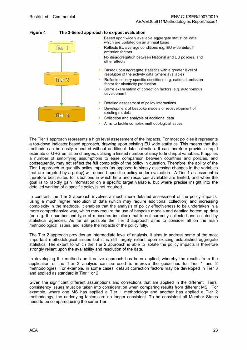
Restricted – Commercial ENV.C.1/SER/2007/0019 AEA/ED05611/Methodologies Report/Issue1
AEA 23
Figure 4 The 3tiered approach to expost evaluation
Tier 1 Tier 1
Tier 3 Tier 3
§ Based upon widely available aggregate statistical data which are updated on an annual basis
§ Reflects EU average conditions e.g. EU wide default emission factors
§ No disaggregation between National and EU policies, and other effects
§ Detailed assessment of policy interactions § Development of bespoke models or redevelopment of
existing models § Collection and analysis of additional data § Aims to tackle complex methodological issues
§ Based upon aggregate statistics with a greater level of resolution of the activity data (where available)
§ Reflects country specific conditions e.g. national emission factor for electricity production
§ Some examination of correction factors, e.g. autonomous development
Tier 2 Tier 2
The Tier 1 approach represents a high level assessment of the impacts. For most policies it represents a topdown indicator based approach, drawing upon existing EU wide statistics. This means that the methods can be easily repeated without additional data collection. It can therefore provide a rapid estimate of GHG emission changes, utilising a limited number of easy to find input variables. It applies a number of simplifying assumptions to ease comparison between countries and policies, and consequently, may not reflect the full complexity of the policy in question. Therefore, the ability of the Tier 1 approach to quantify policy impacts (as opposed to simply assessing changes in the variables that are targeted by a policy) will depend upon the policy under evaluation. A Tier 1 assessment is therefore best suited for situations in which time and resources available are limited, and when the goal is to rapidly gain information on a specific target variable, but where precise insight into the detailed working of a specific policy is not required.
In contrast, the Tier 3 approach involves a much more detailed assessment of the policy impacts, using a much higher resolution of data (which may require additional collection) and increasing complexity in the methods. It enables that the analysis of policy effectiveness to be undertaken in a more comprehensive way, which may require the use of bespoke models and detailed bottom up data (on e.g. the number and type of measures installed) that is not currently collected and collated by statistical agencies. As far as possible the Tier 3 approach aims to consider all on the main methodological issues, and isolate the impacts of the policy fully.
The Tier 2 approach provides an intermediate level of analysis. It aims to address some of the most important methodological issues but it is still largely reliant upon existing established aggregate statistics. The extent to which the Tier 2 approach is able to isolate the policy impacts is therefore strongly reliant upon the availability and resolution of the data.
In developing the methods an iterative approach has been applied, whereby the results from the application of the Tier 3 analysis can be used to improve the guidelines for Tier 1 and 2 methodologies. For example, in some cases, default correction factors may be developed in Tier 3 and applied as standard in Tier 1 or 2.
Given the significant different assumptions and corrections that are applied in the different Tiers, consistency issues must be taken into consideration when comparing results from different MS. For example, where one MS has applied a Tier 1 methodology and another has applied a Tier 2 methodology, the underlying factors are no longer consistent. To be consistent all Member States need to be compared using the same Tier.
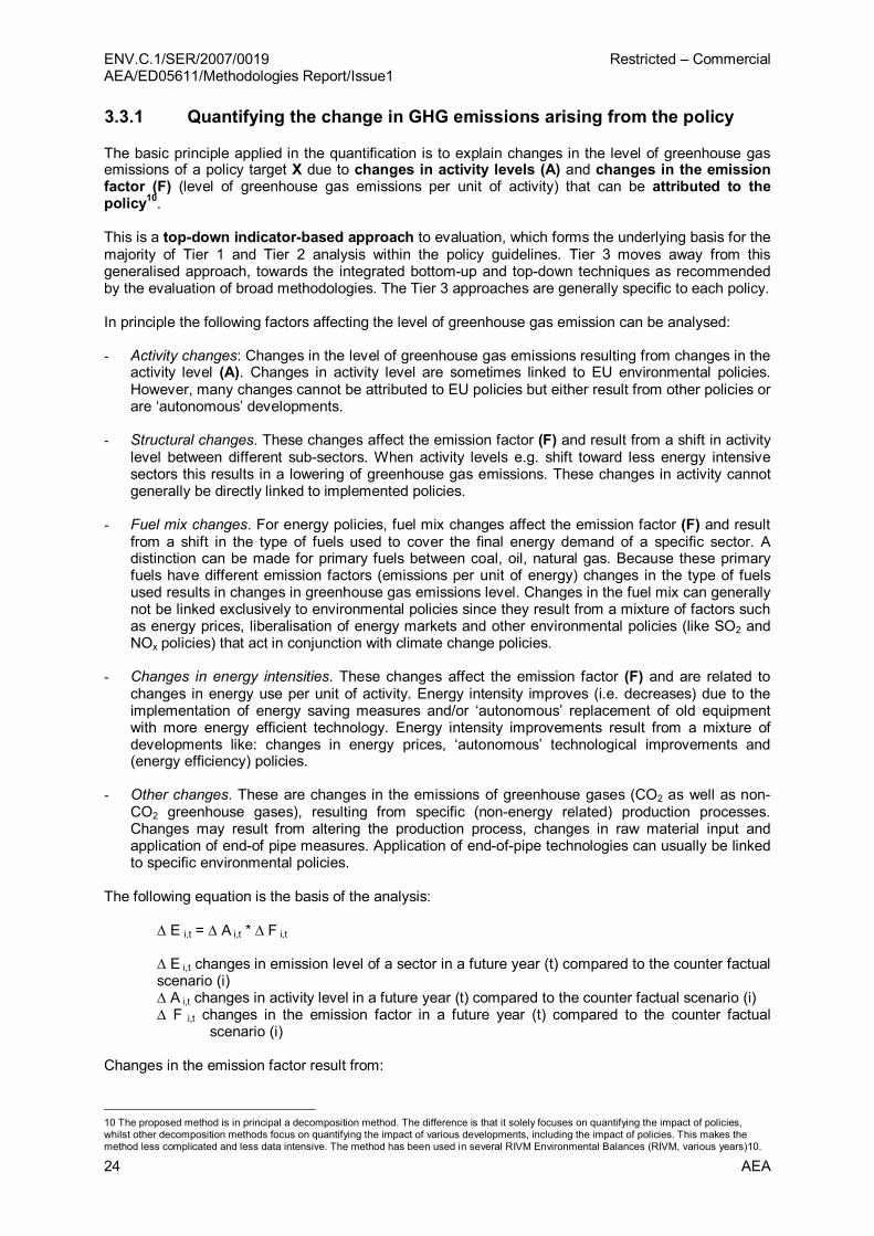
ENV.C.1/SER/2007/0019 Restricted – Commercial AEA/ED05611/Methodologies Report/Issue1
24 AEA
3.3.1 Quantifying the change in GHG emissions arising from the policy
The basic principle applied in the quantification is to explain changes in the level of greenhouse gas emissions of a policy target X due to changes in activity levels (A) and changes in the emission factor (F) (level of greenhouse gas emissions per unit of activity) that can be attributed to the policy 10 .
This is a topdown indicatorbased approach to evaluation, which forms the underlying basis for the majority of Tier 1 and Tier 2 analysis within the policy guidelines. Tier 3 moves away from this generalised approach, towards the integrated bottomup and topdown techniques as recommended by the evaluation of broad methodologies. The Tier 3 approaches are generally specific to each policy.
In principle the following factors affecting the level of greenhouse gas emission can be analysed:
Activity changes: Changes in the level of greenhouse gas emissions resulting from changes in the activity level (A). Changes in activity level are sometimes linked to EU environmental policies. However, many changes cannot be attributed to EU policies but either result from other policies or are ‘autonomous’ developments.
Structural changes. These changes affect the emission factor (F) and result from a shift in activity level between different subsectors. When activity levels e.g. shift toward less energy intensive sectors this results in a lowering of greenhouse gas emissions. These changes in activity cannot generally be directly linked to implemented policies.
Fuel mix changes. For energy policies, fuel mix changes affect the emission factor (F) and result from a shift in the type of fuels used to cover the final energy demand of a specific sector. A distinction can be made for primary fuels between coal, oil, natural gas. Because these primary fuels have different emission factors (emissions per unit of energy) changes in the type of fuels used results in changes in greenhouse gas emissions level. Changes in the fuel mix can generally not be linked exclusively to environmental policies since they result from a mixture of factors such as energy prices, liberalisation of energy markets and other environmental policies (like SO2 and NOx policies) that act in conjunction with climate change policies.
Changes in energy intensities. These changes affect the emission factor (F) and are related to changes in energy use per unit of activity. Energy intensity improves (i.e. decreases) due to the implementation of energy saving measures and/or ‘autonomous’ replacement of old equipment with more energy efficient technology. Energy intensity improvements result from a mixture of developments like: changes in energy prices, ‘autonomous’ technological improvements and (energy efficiency) policies.
Other changes. These are changes in the emissions of greenhouse gases (CO2 as well as non CO2 greenhouse gases), resulting from specific (nonenergy related) production processes. Changes may result from altering the production process, changes in raw material input and application of endof pipe measures. Application of endofpipe technologies can usually be linked to specific environmental policies.
The following equation is the basis of the analysis:
∆ E i,t = ∆ A i,t * ∆ F i,t
∆ E i,t changes in emission level of a sector in a future year (t) compared to the counter factual scenario (i) ∆ A i,t changes in activity level in a future year (t) compared to the counter factual scenario (i) ∆ F i,t changes in the emission factor in a future year (t) compared to the counter factual
scenario (i)
Changes in the emission factor result from:
10 The proposed method is in principal a decomposition method. The difference is that it solely focuses on quantifying the impact of policies, whilst other decomposition methods focus on quantifying the impact of various developments, including the impact of policies. This makes the method less complicated and less data intensive. The method has been used in several RIVM Environmental Balances (RIVM, various years)10.
Restricted – Commercial ENV.C.1/SER/2007/0019 AEA/ED05611/Methodologies Report/Issue1
AEA 25
∆ F i,t = ∆S i,t+∆M i,t+∆I i,t+∆P i,t
∆ F i,t changes in the emission factor in a future year (t) compared to the counter factual scenario (i)
∆ S i,t changes in structure of a sector in a future year (t) compared to the counter factual scenario(i)
∆ M i,t changes in the fuel mix of a sector in a future year (t) compared to the counter factual scenario(i)
∆ I i,t changes in the energy intensity of a sector in a future year (t) compared to the counter factual scenario (i)
∆ P i,t others changes in sector in a future year (t) compared to the counter factual scenario (i)
It must be noted that the formula above describes the approach to policies and measures affecting the energy sector, as they include variables such as fuel mix and energy intensity, which typically effect the level of emission factor in the energy sector. However, the basic activity level/emission factor approach can easily be adapted to other policies. For example, in relation to agricultural emissions whereby the number of animals are used for activity levels and the emissions factor may be affected by changes in the approach to manure management.
3.4 Implementation of the framework The implementation of the tiered framework requires a number of practical choices to be made that may, potentially, have a large effect on the overall results. It is important that the approach taken for each choice is articulated in a transparent and clear way, so that Member States can undertake policy evaluation in a consistent manner and obtain results that are easily understood and interpreted.
This section discusses how the tiered framework and methodological issues have influenced the development of the policy guidelines. It must be noted that that the final development of the guidelines has followed a highly iterative approach with input and comments received from Commission and Member State representatives. In many cases the choice of approach and impact on a particular methodological issue at a given Tier is strongly influenced by what is possible in practice, for example, given limitations on data availability.
The following key issues are addressed in turn.
11 E.g. see http://themes.eea.europa.eu/Sectors_and_activities/energy/indicators/EN09%2C2007.04/EN09_EU25_Policy_effectiveness_20 06.pdf
Composition and decomposition methods Composition/decomposition methods assume simultaneous occurrence of various trends, the outcome being determined by the chosen sequence.
1. The composition method starts from the actual situation in which all effects are included and then calculates what the emissions would have been if effect A had not occurred, and then if effects A and B had not occurred, etc. With this method, every effect is being compared with another baseline. The baseline of effect A is ‘‘the real world’’, the baseline of effect B is ‘‘the real world + effect A’’, etc.
2. The decomposition method starts from the situation in which no effect besides the growth in activity level is included (‘‘frozen efficiency’’), and then calculates what the emissions are if only effect A had occurred, and then if effects A and B had occurred, etc. With this method, every effect is being compared with another baseline too. The baseline of effect A is ‘‘frozen efficiency’’, the baseline of effect B is ‘‘the frozen efficiency + effect A’’, etc. This approach is applied in the environmental balances of the RIVM and indicators produced by the EEA11.
(Gijsen and Oude Lohuis, 2005) undertake a case study in which they analyse the CO2 emissions of the electricity sector in the Netherlands. The different methods result in different outcomes for various developments. In addition to the type of method the sequence in which developments are analysed has an impact on the CO2 effect attributed to the various developments as well, in particular the ‘residual’ effect, which accounts for all other remaining factors.
ENV.C.1/SER/2007/0019 Restricted – Commercial AEA/ED05611/Methodologies Report/Issue1
26 AEA
i) Choice of indicators data § Activity data § Emissions factors (and their impact on the counterfactual) § Consistency with inventory data
ii) Disentangling the policy package
iii) Defining the counterfactual § Autonomous savings § Freeriders (deadweight) § Hidden structural effects § Geographic factors § Direct Rebound effects § Other exogenous factors such as price impacts
iv) Defining the scope of the evaluation § Timing issues § Multiplier effects § Indirect rebound effects
v) Uncertainties and sensitivity analysis
3.4.1 Choice of indicator data
An initial step in the implementation of the methodological framework is to identify a suitable activity and emission factor data that can be used as part of the indicator approach that to quantify the policy impacts, as described in section 3.3.1.
Activity data
Figure 5 below shows the relationship between the resolution of the analysis and the type and amount of data needed to perform the analysis. For example, GDP provides an aggregate level indicator of the economic activity of a country. Since higher economic growth usually implies an increase in energy use and related CO2 emissions, changes in GDP can provide a reasonable indication of greenhouse emissions at a national level. However, GDP may not provide a sufficient proxy for changes in emissions at a higher level of resolution (e.g. emissions within a particular sector of the economy). This requires more disaggregated data on e.g. output or physical activity at sector or even installation level.
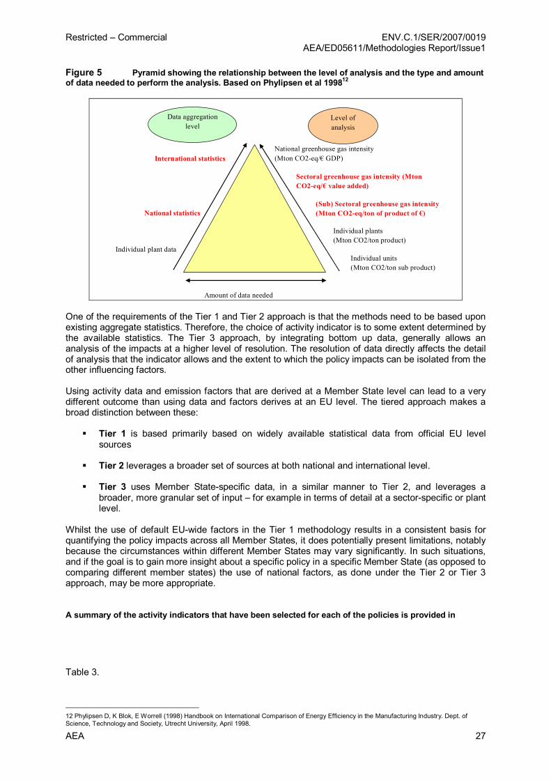
Restricted – Commercial ENV.C.1/SER/2007/0019 AEA/ED05611/Methodologies Report/Issue1
AEA 27
Figure 5 Pyramid showing the relationship between the level of analysis and the type and amount of data needed to perform the analysis. Based on Phylipsen et al 1998 12
International statistics
National statistics
Individual plant data
Amount of data needed
Individual plants (Mton CO2/ton product)
Sectoral greenhouse gas intensity (Mton CO2eq/€ value added)
(Sub) Sectoral greenhouse gas intensity (Mton CO2eq/ton of product of €)
Individual units (Mton CO2/ton sub product)
National greenhouse gas intensity (Mton CO2eq/€ GDP)
Data aggregation level
Level of analysis
One of the requirements of the Tier 1 and Tier 2 approach is that the methods need to be based upon existing aggregate statistics. Therefore, the choice of activity indicator is to some extent determined by the available statistics. The Tier 3 approach, by integrating bottom up data, generally allows an analysis of the impacts at a higher level of resolution. The resolution of data directly affects the detail of analysis that the indicator allows and the extent to which the policy impacts can be isolated from the other influencing factors.
Using activity data and emission factors that are derived at a Member State level can lead to a very different outcome than using data and factors derives at an EU level. The tiered approach makes a broad distinction between these:
§ Tier 1 is based primarily based on widely available statistical data from official EU level sources
§ Tier 2 leverages a broader set of sources at both national and international level.
§ Tier 3 uses Member Statespecific data, in a similar manner to Tier 2, and leverages a broader, more granular set of input – for example in terms of detail at a sectorspecific or plant level.
Whilst the use of default EUwide factors in the Tier 1 methodology results in a consistent basis for quantifying the policy impacts across all Member States, it does potentially present limitations, notably because the circumstances within different Member States may vary significantly. In such situations, and if the goal is to gain more insight about a specific policy in a specific Member State (as opposed to comparing different member states) the use of national factors, as done under the Tier 2 or Tier 3 approach, may be more appropriate.
A summary of the activity indicators that have been selected for each of the policies is provided in
Table 3.
12 Phylipsen D, K Blok, E Worrell (1998) Handbook on International Comparison of Energy Efficiency in the Manufacturing Industry. Dept. of Science, Technology and Society, Utrecht University, April 1998.
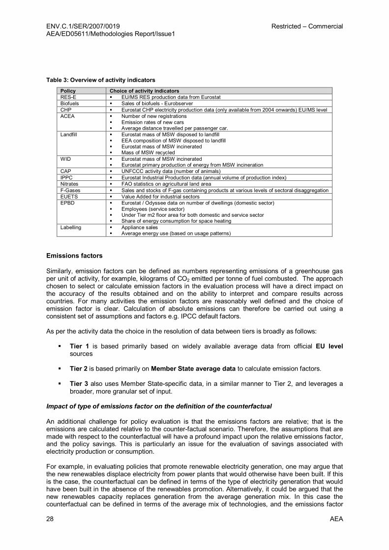
ENV.C.1/SER/2007/0019 Restricted – Commercial AEA/ED05611/Methodologies Report/Issue1
28 AEA
Table 3: Overview of activity indicators
Policy Choice of activity indicators RESE § EU/MS RES production data from Eurostat Biofuels § Sales of biofuels Eurobserver CHP § Eurostat CHP electricity production data (only available from 2004 onwards) EU/MS level ACEA § Number of new registrations
§ Emission rates of new cars § Average distance travelled per passenger car.
Landfill § Eurostat mass of MSW disposed to landfill § EEA composition of MSW disposed to landfill § Eurostat mass of MSW incinerated § Mass of MSW recycled
WID § Eurostat mass of MSW incinerated § Eurostat primary production of energy from MSW incineration
CAP § UNFCCC activity data (number of animals) IPPC § Eurostat Industrial Production data (annual volume of production index) Nitrates § FAO statistics on agricultural land area FGases § Sales and stocks of Fgas containing products at various levels of sectoral disaggregation EUETS § Value Added for industrial sectors EPBD § Eurostat / Odyssee data on number of dwellings (domestic sector)
§ Employees (service sector) § Under Tier m2 floor area for both domestic and service sector § Share of energy consumption for space heating
Labelling § Appliance sales § Average energy use (based on usage patterns)
Emissions factors
Similarly, emission factors can be defined as numbers representing emissions of a greenhouse gas per unit of activity, for example, kilograms of CO2 emitted per tonne of fuel combusted. The approach chosen to select or calculate emission factors in the evaluation process will have a direct impact on the accuracy of the results obtained and on the ability to interpret and compare results across countries. For many activities the emission factors are reasonably well defined and the choice of emission factor is clear. Calculation of absolute emissions can therefore be carried out using a consistent set of assumptions and factors e.g. IPCC default factors.
As per the activity data the choice in the resolution of data between tiers is broadly as follows:
§ Tier 1 is based primarily based on widely available average data from official EU level sources
§ Tier 2 is based primarily on Member State average data to calculate emission factors.
§ Tier 3 also uses Member Statespecific data, in a similar manner to Tier 2, and leverages a broader, more granular set of input.
Impact of type of emissions factor on the definition of the counterfactual
An additional challenge for policy evaluation is that the emissions factors are relative; that is the emissions are calculated relative to the counterfactual scenario. Therefore, the assumptions that are made with respect to the counterfactual will have a profound impact upon the relative emissions factor, and the policy savings. This is particularly an issue for the evaluation of savings associated with electricity production or consumption.
For example, in evaluating policies that promote renewable electricity generation, one may argue that the new renewables displace electricity from power plants that would otherwise have been built. If this is the case, the counterfactual can be defined in terms of the type of electricity generation that would have been built in the absence of the renewables promotion. Alternatively, it could be argued that the new renewables capacity replaces generation from the average generation mix. In this case the counterfactual can be defined in terms of the average mix of technologies, and the emissions factor

Restricted – Commercial ENV.C.1/SER/2007/0019 AEA/ED05611/Methodologies Report/Issue1
AEA 29
calculated on a similar basis. In both cases the emissions factor is therefore the difference between the emissions from renewables generation per unit of output, and the emissions from the alternative technology or mix of technologies.
The emissions savings of renewable energy compared to the alternative new generation capacity technology may be less than if the comparison was with the average emissions from electricity generation (e.g. due to the presence of older, more inefficient, plants in the average energy mix).
A further option for the counterfactual is to look at what generating capacity the new renewable devices will actually replace in the electricity market. For example, hydropower or nuclear plants tend to be used as baseload in most grids, and are therefore are unlikely to be impacted by climate change policies that change demand or promote RES. Typically a fossil fuel is currently used as marginal fuel in most electricity grids. Whilst it may not be possible to accurately calculate the specific marginal fossil plant that would be displaced, correcting the average emissions factor to leave only fossil generation provides a more realistic assessment of the policy’s impact on emissions.
The table below summarizes the broad advantages and disadvantages of the different options
Table 4: Choosing emission factors. Advantages and disadvantages of different options
Type of emissions factor
Advantages Disadvantages
EU Average § Easier to calculate and apply § Consistency across MS
§ May significantly over/underestimate MS savings
MS Average § More accurate assessment of MS savings
§ More effort in calculation § Greater scope of
inconsistencies in calculation Marginal § Potentially more accurate
representation of counterfactual situation
§ Not applicable in all cases § Maybe more subjective to
estimate than calculation of average emission factors and may need to evolve over time
A brief overview of the differing approaches to calculating emissions factors, covering both the choice of data and type in the guidelines is provided in

ENV.C.1/SER/2007/0019 Restricted – Commercial AEA/ED05611/Methodologies Report/Issue1
30 AEA
Table 5.
However, a more detailed discussion of the issues associated with the selection and calculation of an appropriate emission factor is provided in Appendix I. It is strongly recommended that this be read in conjunction with the application of the guidelines, given that the selection of emission factors is a key determinant in the final estimated savings from a policy.
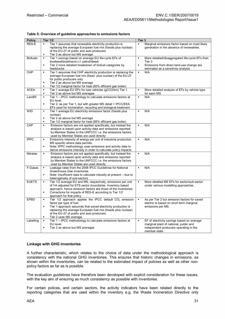
Restricted – Commercial ENV.C.1/SER/2007/0019 AEA/ED05611/Methodologies Report/Issue1
AEA 31
Table 5: Overview of guideline approaches to emissions factors
Policy Tier 1/2 Tier 3 RESE § Tier 1 assumes that renewable electricity production is
replacing the average European fuel mix (fossils plus nuclear) of the EU27 of public and auto producers
§ Tier 2 as above but MS average
§ Marginal emissions factor based on most likely generation in the absence of renewables.
Biofuels § Tier 1 savings based on average EU lifecycle EFs of biodiesel/bioethanol c.f. petrol/diesel
§ Tier 2 more detailed breakdown of biofuel categories by feedstocks
§ More detailed/disaggregated lifecycle EFs than Tier 3
§ Emissions from direct landuse change are estimated as a sensitivity analysis
CHP § Tier 1 assumes that CHP electricity production is replacing the average European fuel mix (fossil plus nuclear) of the EU27 for public producers only
§ Tier 2 as above but MS average § Tier 1/2 marginal factor for heat (85% efficient gas boiler)
§ N/A
ACEA § Tier 1 average EU EFs for new vehicles (gCO2/km) Tier 1 § Tier 2 as above but MS averages
§ More detailed analysis of EFs by vehicle type for each MS
Landfill § Tier 1 – IPCC methodology to calculate emissions factors at EU level.
§ Tier 2, as per Tier 1, but with greater MS detail + IPCC/EEA EFs used for incineration, recycling and biological treatment
§ N/A
WID § Tier 1 average EU electricity emissions factor (fossils plus nuclear)
§ Tier 2 as above but MS average § Tier 1/2 marginal factor for heat (85% efficient gas boiler)
§ N/A
CAP § Emission factors are not applied specifically, but instead the analysis is based upon activity data and emissions reported by Member States to the UNFCCC i.e. the emissions factors used by Member States are used directly
§ N/A
IPPC § Emissions intensity of energy per unit of industrial production. MS specific where data permits.
§ Note: IPPC methodology uses emissions and activity data to derive emissions intensity in order to calculate policy impacts
§ N/A
Nitrates § Emission factors are not applied specifically, but instead the analysis is based upon activity data and emissions reported by Member States to the UNFCCC i.e. the emissions factors used by Member States are used directly
§ N/A
FGases § Leakage rates from the 2006 IPCC Guidelines for National Greenhouse Gas Inventories
§ Note: Insufficient data to calculate robustly at present – due to heterogeneity of subsectors
§ N/A
EUETS § Tier 1/2 average EU and MS, respectively, emissions per unit of VA adjusted for ETS sector boundaries. Inventory based approach, hence emission factors are those of the inventories.
§ Corrections for impacts of RESE according to Tier 1/2 approach for that policy
§ More detailed MS EFs for sector/subsector under various modelling approaches.
EPBD § Tier 1/2 approach applies the IPCC default CO2 emission factor per type of fuel.
§ Tier 1 approach assumes that saved electricity production is replacing the average European fuel mix (fossils plus nuclear) of the EU27 of public and auto producers.
§ Tier 2 uses MS average.
§ As per Tier 2 but emission factors for saved electric is based on short term marginal emissions per MS.
Labelling § Tier 1 – IPCC methodology to calculate emissions factors at EU level.
§ Tier 2 as above but MS averages
§ EF of electricity savings based on average marginal plant of national, public and independent producers operating in the member state
Linkage with GHG inventories
A further characteristic, which relates to the choice of data under the methodological approach is consistency with the national GHG inventories. This ensures that historic changes in emissions, as shown within the inventories, can be related to the estimated impact of policies as well as other non policy factors as far as is possible.
The evaluation guidelines have therefore been developed with explicit consideration for these issues, with the key aim of ensuring as much consistency as possible with inventories.
For certain polices, and certain sectors, the activity indicators have been related directly to the reporting categories that are used within the inventory e.g. the Waste Incineration Directive only

ENV.C.1/SER/2007/0019 Restricted – Commercial AEA/ED05611/Methodologies Report/Issue1
32 AEA
affects one category within the inventory. However, for other polices the relationship is more complex as the polices may have an impact upon multiple categories. In other cases differences in how sectors are defined within the inventories and within regulations may affect the compatibility. For example, EU ETS categories do not directly match the IPCC categories. Sometimes only part of the category is covered and sector coverage is different between some of the member states.
Relating the estimated policy impacts to the observed changes in national inventories is complicated further by a number of other factors, including:
§ Policy overlaps between EU and national policies, which may lead to potential double counting and overestimation of the impact (discussed further below).
§ Uncertainties in the estimate of the impact under Tier 1 compared to higher tiers – e.g. the use of EU averages under Tier 1, which may be too conservative/rewarding for a particular Member State.
§ The level of disaggregation of the impact possible under lower Tiers. For example whether it is possible to apportion the impact between the multiple IPCC categories, which may require sectoral level data that is not available under Tier 1 / 2.
3.4.2 Disentangling the policy package
Policies under the ECCP can be divided into regulations and directives. A regulation is a legislative act of the European Union which becomes immediately enforceable as law in all member states simultaneously. A directive is a legislative act of the European Union which requires member states to achieve a particular result without dictating the means of achieving that result. When adopted, directives give member states a timetable for the implementation of the intended outcome. Occasionally the laws of a member state may already comply with this outcome and the state involved would only be required to keep their laws in place. But more commonly member states are required to make changes to their laws in order for the directive to be implemented correctly. This, however, complicates the analysis as it will be hard to separate the impact of ECCPs from national policies that already were in place before the Directive came into force.
As described previously a measures mapping approach is useful to help to identify the measures that interact or overlap with the policy or regulation in question. This technique is also useful for understanding if and how these measures will influence the activity indicator that has been selected for use in the evaluation, and therefore the potential for double counting.
In relation to our tiered methodological framework, ideally the analysis at each Tier would assess the impact of only the policy under consideration. However, limitations in data availability preclude the possibility to clearly differentiate the impact of, for example, national versus EU policies for some of the directives, and this links directly to the choice of indicator data in section 3.4.1.
• Under Tier 1 and Tier 2, because there is a need to use aggregate level data and a relatively simple topdown indicator approach based on activity level/emissions factors, it is not possible to differentiate between separate policy factors that may also be simultaneously affecting these elements. For example, the activity data for the RESE directive is the production of renewable electricity at the member state level, and both their own policies and any EUlevel policy will directly affect this variable. Hence under these Tiers it is generally not possible to differentiate between EU only and Member State level policy. In addition, it is often not possible under these Tiers to differentiate between overlapping EUlevel policy instruments.
• The more detailed integrated approach under Tier 3, both in terms of the selection of data and the more detailed analytical approach (i.e. no longer based solely on topdown indicatorbased approach) allows these overlaps and synergies to be explored in more detail.
A brief overview of the differing approaches to addressing policy overlaps taken in the guidelines is provided in

Restricted – Commercial ENV.C.1/SER/2007/0019 AEA/ED05611/Methodologies Report/Issue1
AEA 33
Table 6.
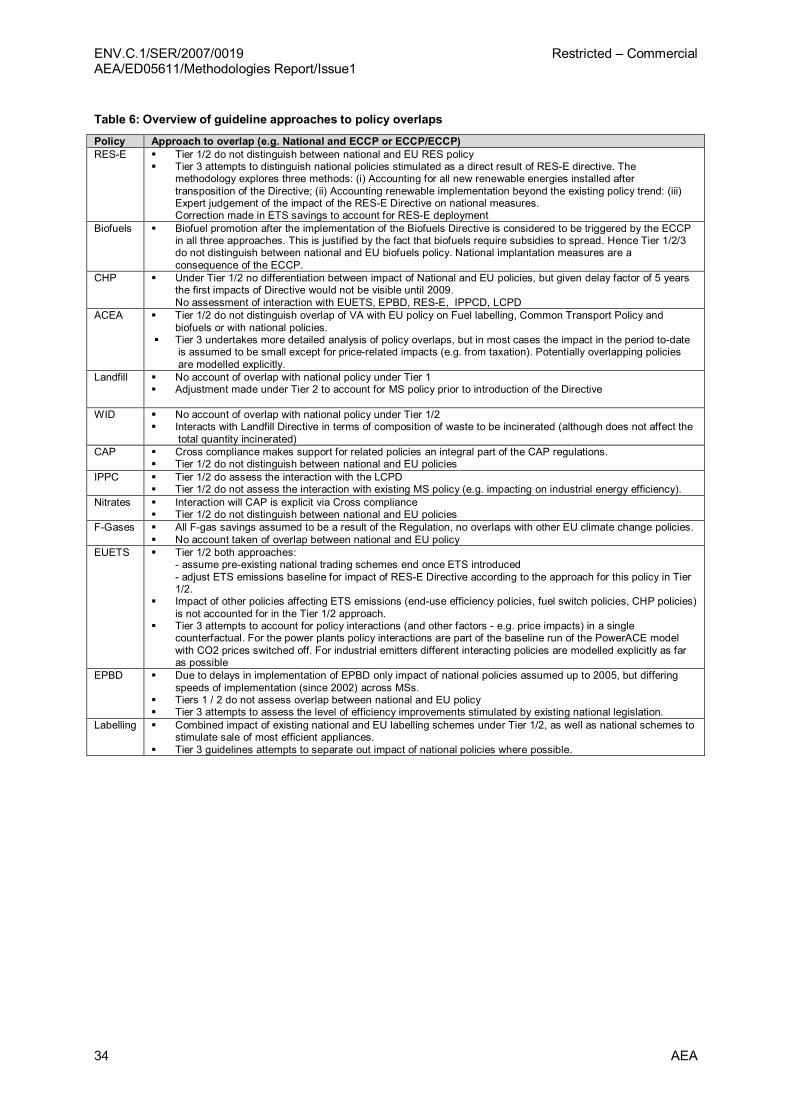
ENV.C.1/SER/2007/0019 Restricted – Commercial AEA/ED05611/Methodologies Report/Issue1
34 AEA
Table 6: Overview of guideline approaches to policy overlaps
Policy Approach to overlap (e.g. National and ECCP or ECCP/ECCP) RESE § Tier 1/2 do not distinguish between national and EU RES policy
§ Tier 3 attempts to distinguish national policies stimulated as a direct result of RESE directive. The methodology explores three methods: (i) Accounting for all new renewable energies installed after transposition of the Directive; (ii) Accounting renewable implementation beyond the existing policy trend: (iii) Expert judgement of the impact of the RESE Directive on national measures. Correction made in ETS savings to account for RESE deployment
Biofuels § Biofuel promotion after the implementation of the Biofuels Directive is considered to be triggered by the ECCP in all three approaches. This is justified by the fact that biofuels require subsidies to spread. Hence Tier 1/2/3 do not distinguish between national and EU biofuels policy. National implantation measures are a consequence of the ECCP.
CHP § Under Tier 1/2 no differentiation between impact of National and EU policies, but given delay factor of 5 years the first impacts of Directive would not be visible until 2009. No assessment of interaction with EUETS, EPBD, RESE, IPPCD, LCPD
ACEA § Tier 1/2 do not distinguish overlap of VA with EU policy on Fuel labelling, Common Transport Policy and biofuels or with national policies.
§ Tier 3 undertakes more detailed analysis of policy overlaps, but in most cases the impact in the period todate is assumed to be small except for pricerelated impacts (e.g. from taxation). Potentially overlapping policies are modelled explicitly.
Landfill § No account of overlap with national policy under Tier 1 § Adjustment made under Tier 2 to account for MS policy prior to introduction of the Directive
WID § No account of overlap with national policy under Tier 1/2 § Interacts with Landfill Directive in terms of composition of waste to be incinerated (although does not affect the
total quantity incinerated) CAP § Cross compliance makes support for related policies an integral part of the CAP regulations.
§ Tier 1/2 do not distinguish between national and EU policies IPPC § Tier 1/2 do assess the interaction with the LCPD
§ Tier 1/2 do not assess the interaction with existing MS policy (e.g. impacting on industrial energy efficiency). Nitrates § Interaction will CAP is explicit via Cross compliance
§ Tier 1/2 do not distinguish between national and EU policies FGases § All Fgas savings assumed to be a result of the Regulation, no overlaps with other EU climate change policies.
§ No account taken of overlap between national and EU policy EUETS § Tier 1/2 both approaches:
assume preexisting national trading schemes end once ETS introduced adjust ETS emissions baseline for impact of RESE Directive according to the approach for this policy in Tier 1/2.
§ Impact of other policies affecting ETS emissions (enduse efficiency policies, fuel switch policies, CHP policies) is not accounted for in the Tier 1/2 approach.
§ Tier 3 attempts to account for policy interactions (and other factors e.g. price impacts) in a single counterfactual. For the power plants policy interactions are part of the baseline run of the PowerACE model with CO2 prices switched off. For industrial emitters different interacting policies are modelled explicitly as far as possible
EPBD § Due to delays in implementation of EPBD only impact of national policies assumed up to 2005, but differing speeds of implementation (since 2002) across MSs.
§ Tiers 1 / 2 do not assess overlap between national and EU policy § Tier 3 attempts to assess the level of efficiency improvements stimulated by existing national legislation.
Labelling § Combined impact of existing national and EU labelling schemes under Tier 1/2, as well as national schemes to stimulate sale of most efficient appliances.
§ Tier 3 guidelines attempts to separate out impact of national policies where possible.

Restricted – Commercial ENV.C.1/SER/2007/0019 AEA/ED05611/Methodologies Report/Issue1
AEA 35
3.4.3 Defining the counterfactual
Aside from the impact of the policy itself there are a range of other factors that will impact on changes to GHG emissions that ideally need to be accounted for in the counterfactual itself or used to correct the final estimates of policy savings – i.e. the net policy impact.
Autonomous development
As described in Section 2.2.2 autonomous progress relates to range of interrelated factors that influence the counterfactual trend in emissions, but are not captured within the scope of the policy evaluation. This may include, for example, the impact of autonomous technological improvement (i.e. innovation in technology), autonomous policy development (i.e. savings arising as a result of previous policies), or autonomous behaviour (where an activity would have occurred anyway, but has instead occurred in relation to a specific policy). Autonomous progress has been considered in the following ways within the guidance:
• In the Tier 1 approach autonomous development is assumed to be zero for all policies. Effectively this means that all savings calculated under the Tier 1 approach are attributed to the policy. For policy where autonomous progress is likely to deliver a reduction in emissions the results derived under this approach will, therefore, represent an overestimate of the true policy impacts.
• In the Tier 2 approach autonomous development has been corrected for where the effects can be clearly defined and isolated using existing statistics. This may involve the linear extrapolation of the historic trends in efficiency. However, for certain polices this may not necessarily capture the full complexity of the issue. For example under the Labelling Directive, the autonomous improvement in appliance efficiency is to some extent offset by trends towards larger appliances (i.e. structural changes are also playing an important role in the observed savings).
In some cases other modifications are made to the activity data directly to account for autonomous developments. For example, the RES Directive guidance assume that all cost effective technologies (only large hydro in this case) are excluded from the policy impacts, as these autonomous developments would have occurred anyway.
• In the Tier 3 approach more detailed analysis of autonomous savings is generally considered. For some policies the approach is similar to that employed within a Tier 2, relying upon linear extrapolation. However, the Tier 3 guidelines more explicitly explore so of the interactions with the other variable. For example, the impact of the energy label itself compared to other factors such as energy prices, changes in household income, etc.
Hidden structural effects
The extent to which structural effects are effectively uncorrected (i.e. hidden) is strongly related to the resolution of the activity and emissions data that is used in the evaluation.
• In the Tier 1 approach no corrections have been made for the influence of hidden structural effects on the activity indicator. Therefore the extent to which this is an issue is entirely dependent upon the resolution of the activity indicator.
• In the Tier 2 approach corrections are made where the structural effects are known and the statistical data allows. For example, the effect of dieselisation of the vehicle stock has been adjusted for in the guidance relating to the voluntary agreement for passenger cars.
• As far as possible, known structural effects are fully corrected for in the Tier 3 approach. This may involve the collection of new data or calibration with alternative data sources. For example, the RES Directive guidance takes into account the replacement of existing renewables capacity as a result of the policy (without which the policy impact would be underestimated in this specific case).
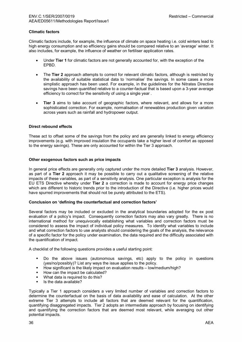
ENV.C.1/SER/2007/0019 Restricted – Commercial AEA/ED05611/Methodologies Report/Issue1
36 AEA
Climatic factors
Climatic factors include, for example, the influence of climate on space heating i.e. cold winters lead to high energy consumption and so efficiency gains should be compared relative to an ‘average’ winter. It also includes, for example, the influence of weather on fertiliser application rates.
• Under Tier 1 for climatic factors are not generally accounted for, with the exception of the EPBD.
• The Tier 2 approach attempts to correct for relevant climatic factors, although is restricted by the availability of suitable statistical data to ‘normalise’ the savings. In some cases a more simplistic approach has been used. For example, in the guidelines for the Nitrates Directive savings have been quantified relative to a counterfactual that is based upon a 3year average efficiency to correct for the sensitivity of using a single year .
• Tier 3 aims to take account of geographic factors, where relevant, and allows for a more sophisticated correction. For example, normalisation of renewables production given variation across years such as rainfall and hydropower output.
Direct rebound effects
These act to offset some of the savings from the policy and are generally linked to energy efficiency improvements (e.g. with improved insulation the occupants take a higher level of comfort as opposed to the energy savings). These are only accounted for within the Tier 3 approach.
Other exogenous factors such as price impacts
In general price effects are generally only captured under the more detailed Tier 3 analysis. However, as part of a Tier 2 approach it may be possible to carry out a qualitative screening of the relative impacts of these variables, as part of a sensitivity analysis. One particular exception is analysis for the EU ETS Directive whereby under Tier 2 a correction is made to account for energy price changes which are different to historic trends prior to the introduction of the Directive (i.e. higher prices would have spurred improvements that should not be purely attributed to the ETS).
Conclusion on ‘defining the counterfactual and correction factors’
Several factors may be included or excluded in the analytical boundaries adopted for the ex post evaluation of a policy’s impact. Consequently correction factors may also vary greatly. There is no international method for unequivocally establishing what variables and correction factors must be considered to assess the impact of individual policy measures. To identify what variables to include and what correction factors to use analysts should considering the goals of the analysis, the relevance of a specific factor for the policy under examination, the data required and the difficulty associated with the quantification of impact.
A checklist of the following questions provides a useful starting point:
§ Do the above issues (autonomous savings, etc) apply to the policy in questions (yes/no/possibly)? List any ways the issue applies to the policy.
§ How significant is the likely impact on evaluation results – low/medium/high? § How can the impact be calculated? § What data is required to do this? § Is the data available?
Typically a Tier 1 approach considers a very limited number of variables and correction factors to determine the counterfactual on the basis of data availability and ease of calculation. At the other extreme Tier 3 attempts to include all factors that are deemed relevant for the quantification, quantifying disaggregated impacts. Tier 2 adopts an intermediate approach by focusing on identifying and quantifying the correction factors that are deemed most relevant, while averaging out other potential impacts.

Restricted – Commercial ENV.C.1/SER/2007/0019 AEA/ED05611/Methodologies Report/Issue1
AEA 37
A brief overview of the differing approaches to defining the counterfactual and addressing other correction factors is provided in Table 7.
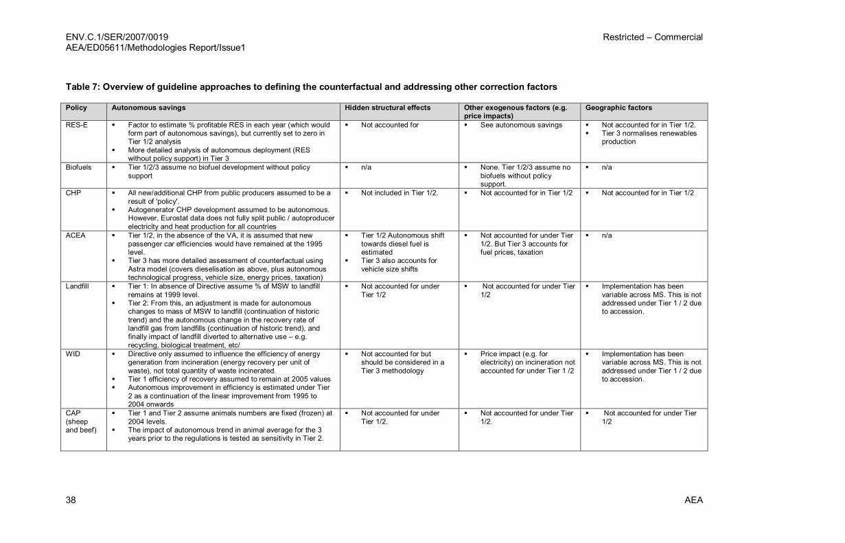
ENV.C.1/SER/2007/0019 Restricted – Commercial AEA/ED05611/Methodologies Report/Issue1
38 AEA
Table 7: Overview of guideline approaches to defining the counterfactual and addressing other correction factors
Policy Autonomous savings Hidden structural effects Other exogenous factors (e.g. price impacts)
Geographic factors
RESE § Factor to estimate % profitable RES in each year (which would form part of autonomous savings), but currently set to zero in Tier 1/2 analysis
§ More detailed analysis of autonomous deployment (RES without policy support) in Tier 3
§ Not accounted for § See autonomous savings § Not accounted for in Tier 1/2. § Tier 3 normalises renewables
production
Biofuels § Tier 1/2/3 assume no biofuel development without policy support
§ n/a § None. Tier 1/2/3 assume no biofuels without policy support.
§ n/a
CHP § All new/additional CHP from public producers assumed to be a result of 'policy'.
§ Autogenerator CHP development assumed to be autonomous. However, Eurostat data does not fully split public / autoproducer electricity and heat production for all countries
§ Not included in Tier 1/2. § Not accounted for in Tier 1/2 § Not accounted for in Tier 1/2
ACEA § Tier 1/2, in the absence of the VA, it is assumed that new passenger car efficiencies would have remained at the 1995 level.
§ Tier 3 has more detailed assessment of counterfactual using Astra model (covers dieselisation as above, plus autonomous technological progress, vehicle size, energy prices, taxation)
§ Tier 1/2 Autonomous shift towards diesel fuel is estimated
§ Tier 3 also accounts for vehicle size shifts
§ Not accounted for under Tier 1/2. But Tier 3 accounts for fuel prices, taxation
§ n/a
Landfill § Tier 1: In absence of Directive assume % of MSW to landfill remains at 1999 level.
§ Tier 2: From this, an adjustment is made for autonomous changes to mass of MSW to landfill (continuation of historic trend) and the autonomous change in the recovery rate of landfill gas from landfills (continuation of historic trend), and finally impact of landfill diverted to alternative use – e.g. recycling, biological treatment, etc/
§ Not accounted for under Tier 1/2
§ Not accounted for under Tier 1/2
§ Implementation has been variable across MS. This is not addressed under Tier 1 / 2 due to accession.
WID § Directive only assumed to influence the efficiency of energy generation from incineration (energy recovery per unit of waste), not total quantity of waste incinerated.
§ Tier 1 efficiency of recovery assumed to remain at 2005 values § Autonomous improvement in efficiency is estimated under Tier
2 as a continuation of the linear improvement from 1995 to 2004 onwards
§ Not accounted for but should be considered in a Tier 3 methodology
§ Price impact (e.g. for electricity) on incineration not accounted for under Tier 1 /2
§ Implementation has been variable across MS. This is not addressed under Tier 1 / 2 due to accession.
CAP (sheep and beef)
§ Tier 1 and Tier 2 assume animals numbers are fixed (frozen) at 2004 levels.
§ The impact of autonomous trend in animal average for the 3 years prior to the regulations is tested as sensitivity in Tier 2.
§ Not accounted for under Tier 1/2.
§ Not accounted for under Tier 1/2.
§ Not accounted for under Tier 1/2
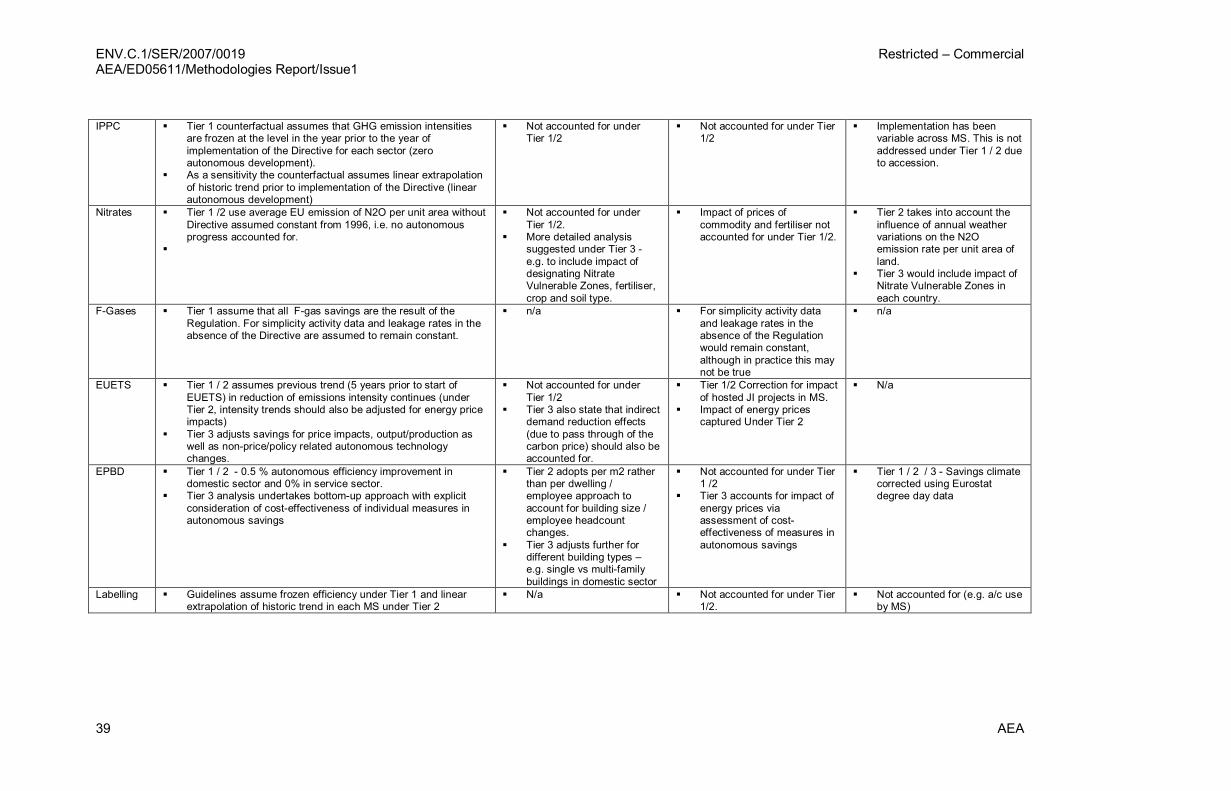
ENV.C.1/SER/2007/0019 Restricted – Commercial AEA/ED05611/Methodologies Report/Issue1
39 AEA
IPPC § Tier 1 counterfactual assumes that GHG emission intensities are frozen at the level in the year prior to the year of implementation of the Directive for each sector (zero autonomous development).
§ As a sensitivity the counterfactual assumes linear extrapolation of historic trend prior to implementation of the Directive (linear autonomous development)
§ Not accounted for under Tier 1/2
§ Not accounted for under Tier 1/2
§ Implementation has been variable across MS. This is not addressed under Tier 1 / 2 due to accession.
Nitrates § Tier 1 /2 use average EU emission of N2O per unit area without Directive assumed constant from 1996, i.e. no autonomous progress accounted for.
§
§ Not accounted for under Tier 1/2.
§ More detailed analysis suggested under Tier 3 e.g. to include impact of designating Nitrate Vulnerable Zones, fertiliser, crop and soil type.
§ Impact of prices of commodity and fertiliser not accounted for under Tier 1/2.
§ Tier 2 takes into account the influence of annual weather variations on the N2O emission rate per unit area of land.
§ Tier 3 would include impact of Nitrate Vulnerable Zones in each country.
FGases § Tier 1 assume that all Fgas savings are the result of the Regulation. For simplicity activity data and leakage rates in the absence of the Directive are assumed to remain constant.
§ n/a § For simplicity activity data and leakage rates in the absence of the Regulation would remain constant, although in practice this may not be true
§ n/a
EUETS § Tier 1 / 2 assumes previous trend (5 years prior to start of EUETS) in reduction of emissions intensity continues (under Tier 2, intensity trends should also be adjusted for energy price impacts)
§ Tier 3 adjusts savings for price impacts, output/production as well as nonprice/policy related autonomous technology changes.
§ Not accounted for under Tier 1/2
§ Tier 3 also state that indirect demand reduction effects (due to pass through of the carbon price) should also be accounted for.
§ Tier 1/2 Correction for impact of hosted JI projects in MS.
§ Impact of energy prices captured Under Tier 2
§ N/a
EPBD § Tier 1 / 2 0.5 % autonomous efficiency improvement in domestic sector and 0% in service sector.
§ Tier 3 analysis undertakes bottomup approach with explicit consideration of costeffectiveness of individual measures in autonomous savings
§ Tier 2 adopts per m2 rather than per dwelling / employee approach to account for building size / employee headcount changes.
§ Tier 3 adjusts further for different building types – e.g. single vs multifamily buildings in domestic sector
§ Not accounted for under Tier 1 /2
§ Tier 3 accounts for impact of energy prices via assessment of cost effectiveness of measures in autonomous savings
§ Tier 1 / 2 / 3 Savings climate corrected using Eurostat degree day data
Labelling § Guidelines assume frozen efficiency under Tier 1 and linear extrapolation of historic trend in each MS under Tier 2
§ N/a § Not accounted for under Tier 1/2.
§ Not accounted for (e.g. a/c use by MS)

ENV.C.1/SER/2007/0019 Restricted – Commercial AEA/ED05611/Methodologies Report/Issue1
40 AEA
3.4.4 Defining the scope of the evaluation
Timing issues
These are linked to the implementation of the Directive and the timing of the impacts. The two issues are a) time delay, whereby the impact from the Directive does not occur immediately but a number of years after its introduction b) an announcement effect, whereby the response to the policy is made prior to its formal introduction, but which should still be attributed to the policy. Not accounting for these would lead to an overestimate of policy savings in the first case and an underestimate in the latter case.
• Timing is generally not accounted for in Tier 1 approach (i.e. a delay of 0 years is assumed), however, in some cases where empirical evidence is sufficient this may be incorporated on a generic basis.
• In the Tier 2 approach timing has been corrected for on a Member State specific basis, where appropriate. For example, the timing of implementation of the Nitrates Directive has been highly variable between Member States, so the start date from which the policy impacts have been quantified have been adjusted accordingly.
• A further complication, as mentioned above in the section on policy overlaps, is any time lag in the impact of existing national policies. This is not addressed in the Tier 1 / 2 approach, but more detailed analysis of timing issues should be undertaken as part of a Tier 3 approach.
Table 8: Overview of guideline approaches to timing issues
Policy Timing issues – e.g. delay factor before any impact of Directive RESE § No delay factor on impact of Directive Biofuels § No delay factor on impact of Directive CHP § At present data only starts in 2004. In current results additional savings from CHP in 2005/6 relative to 2004
are assumed to be a result of policy as data is not sufficient to establish level of 'additional' CHP from earlier base year (e.g. 1990) Also, impact of Directive itself is unlikely to occur from 2004 as it is not yet fully implemented.
ACEA § Brought forward 4 years (starting in 1995) due to announcement effect. Landfill § Delay time of 2 years (assume impact from 2001 onwards) WID § Delay to 2005, year of implementation for existing plant CAP § MS specific delay time applied in Tier 2. IPPC § No. Directive date is 1996. 1st implementation (new or amended installations) due 1999. Existing installations
by 2007. § Methodology assumes first year of impact is 1999. This divide between existing and new is not yet addressed.
Nitrates § MS specific delay time applied in Tier 2. FGases § Assumed to be least 2 years from entry into force (2006) Delay in data availability will delay the applicability of
evaluation processes EUETS § No delay time assumed EPBD § No delay time, but EPBD not fully implemented in all MS yet (potentially a 5 year delay, but not implemented
explicitly in guidelines at present) Labelling § Assumed to be zero
Multiplier effects
Such as greater innovation induced by the policy measure are not currently addressed under any Tier (including 3), due to the difficulty in reliably quantifying their impacts.
Indirect rebound effects
Again these are not currently addressed under any Tier (including 3), due to the difficulty in reliably quantifying their impacts.

ENV.C.1/SER/2007/0019 Restricted – Commercial AEA/ED05611/Methodologies Report/Issue1
AEA 41
3.4.5 Uncertainty and Sensitivity Analysis
Whilst a standardised set of assumptions is important to ensure comparability between the estimates of policy impact for different Member States, specific national circumstances could be tested by means of sensitivity analysis (the altering of input variables one by one to understand the impact on estimated emissions saving).
In addition, areas of uncertainty (both in terms of methodological approach and available data) can vary between the policies, requiring sensitivity analysis to performed on different variables. Key areas of uncertainty for each of the guidelines are summarised in the table below. The impact of some of these on emissions savings from the specific policies are explored within the results sections of the separate, main report from this project.
Table 9: Key areas of uncertainty in guidelines
Policy Area RESE § Main uncertainty in the tier 1 / 2 approach arises from the estimate of the factor X (share of renewable electricity
that is profitable on the country level) § Next uncertainty is related to the uncertainly in the energy statistics used, and the use of default emission
factors. Biofuels § Main uncertainty in the tier 1 approach arises from application of the default life cycle emission factors for
biofuels § Next uncertainty is related to the uncertainly in the statistics on the consumption and production of biofuels and
missing information on the details of the feedstocks, especially also from imported biofuels CHP § Various issues to do with existing data on CHP production, fuel use, etc.
§ Assumptions on standard factors for CHP/boiler efficiency. ACEA § Main uncertainty is on the level of autonomous improvement in the absence of the policy
§ Other uncertainties to be considered include: Scrapping rate. The approach assumes that new registrations will only replace the oldest cars in the vehicle
fleet The tier 1 analysis assumes that new cars drive the average vehicle kms calculated for the entire
passenger car fleet in a specific year. There is evidence that new cars would travel further than the average across the whole fleet.
The impact of increases in the mass of passenger cars on the autonomous efficiency improvement. Landfill § The main uncertainty in the tier 1 approach arises from the assumption that the proportion of the mass of MSW
generated that is disposed of to landfill and its emission rate would remain at 2001 levels in the absence of the policy.
WID § The main uncertainty in the tier 1 approach arises from the assumption that the rate of energy recovery would remain at 2005 levels in the absence of the policy.
CAP § The principle uncertainty is the development of the counterfactual. Particularly animal numbers and emissions per head.
§ There is also a large uncertainty in the emission factors and not all emissions sources are fully capture. IPPC § The principal uncertainty of this analysis lies in the assumption of a linear trend in emissions intensity prior to the
implementation of the directive and the continuation of that trend to the present – i.e. the autonomous improvement trend.
Nitrates § The principle uncertainty arises from the counterfactual for evolution of N2O emissions per area of land in the absence of the Nitrates Directive. In particular under Tier 1 it does not take into account the influence of other policies or other exogenous factors on the indicator.
FGases § The main uncertainty in the tier 1 approach arises from the heterogeneity of the affected sectors. There is also limited/uncertain activity and emissions factor data.
EUETS § The main uncertainty arises in: The inconsistency of sector boundaries between ETS/nonETS participants and boundaries distinguished in
modelling/statistics The lack of empirical basis for elasticities to estimate demand reduction effects in the industrial sector or the
passthough factors for electricity prices and industrial products. The effect of changing energy prices The effect of other factors driving carbon intensity over time, particularly policy overlaps, which change
during the period used for establishing the historic trend or the evaluation period. EPBD § Uncertainty in the numbers on the share of energy used for space heating in the residential and service sector.
§ Energy statistics on the service sector are usually not of a very high quality and includes relatively large uncertainties
§ Assumption with respect to autonomous efficiency improvement of 0.5% per year in the residential sector and 0% per year for the service sector.
§ National policies are at varying levels of implementation and reductions may not have occurred as a result of the Directive to date.
§ Whether or not comfort factors are to be included in the analysis Labelling § Lack of data availability for individual appliances and uncertainty over total appliance sales and average usage
per annum, particular when differentiated at MS level. § Uncertainty with respect to use of average or marginal emission factors for electricity
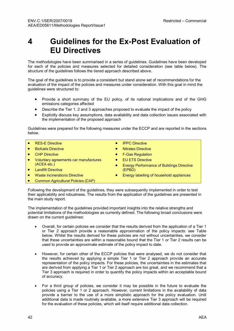
ENV.C.1/SER/2007/0019 Restricted – Commercial AEA/ED05611/Methodologies Report/Issue1
42 AEA
4 Guidelines for the ExPost Evaluation of EU Directives
The methodologies have been summarised in a series of guidelines. Guidelines have been developed for each of the policies and measures selected for detailed consideration (see table below). The structure of the guidelines follows the tiered approach described above.
The goal of the guidelines is to provide a consistent but stand alone set of recommendations for the evaluation of the impact of the policies and measures under consideration. With this goal in mind the guidelines were structured to:
• Provide a short summary of the EU policy, of its national implications and of the GHG emissions categories affected
• Describe the Tier 1, 2 and 3 approaches proposed to evaluate the impact of the policy • Explicitly discuss key assumptions, data availability and data collection issues associated with
the implementation of the proposed approach
Guidelines were prepared for the following measures under the ECCP and are reported in the sections below.
• RESE Directive • Biofuels Directive • CHP Directive • Voluntary agreements car manufactures
(ACEA etc.) • Landfill Directive • Waste Incinerations Directive • Common Agricultural Policies (CAP)
• IPPC Directive • Nitrates Directive • FGas Regulation • EU ETS Directive • Energy Performance of Buildings Directive
(EPBD) • Energy labelling of household appliances
Following the development of the guidelines, they were subsequently implemented in order to test their applicability and robustness. The results from the application of the guidelines are presented in the main study report.
The implementation of the guidelines provided important insights into the relative strengths and potential limitations of the methodologies as currently defined. The following broad conclusions were drawn on the current guidelines:
• Overall, for certain policies we consider that the results derived from the application of a Tier 1 or Tier 2 approach provide a reasonable approximation of the policy impacts: see Table below. Whilst the results derived for these policies are not without uncertainties, we consider that these uncertainties are within a reasonable bound that the Tier 1 or Tier 2 results can be used to provide an approximate estimate of the policy impact to date.
• However, for certain other of the ECCP policies that were analysed, we do not consider that the results achieved by applying a simple Tier 1 or Tier 2 approach provide an accurate representation of the policy impacts. For these policies, the uncertainties in the estimates that are derived from applying a Tier 1 or Tier 2 approach are too great, and we recommend that a Tier 3 approach is required in order to quantify the policy impacts within an acceptable bound of accuracy.
• For a third group of policies, we consider it may be possible in the future to evaluate the policies using a Tier 1 or 2 approach. However, current limitations in the availability of data provide a barrier to the use of a more simplistic approach for the policy evaluation. Until additional data is made routinely available, a more extensive Tier 3 approach will be required for the evaluation of these policies, which will itself require additional data collection.

ENV.C.1/SER/2007/0019 Restricted – Commercial AEA/ED05611/Methodologies Report/Issue1
AEA 43
Table E1: Suitability of the tiered methodologies for evaluating the impacts of individual policies
Policies for which a Tier 1 and 2 methodology can be currently used to produce reasonable estimates of policy impact
Policies for which a Tier 1 and 2 methodology could in the future be used to produce reasonable estimates of policy impact
Policies for which a Tier 3 methodology is required due to the complexity of methodology or high resolution of data required
RESE Directive Labelling Directive ACEA agreement Landfill Directive Biofuels Directive 13
Nitrates Directive* CHP Directive* Energy Performance of Buildings Directive*
EU ETS* IPPC* Common Agricultural Policy (CAP) reform* Fgas Regulations* Waste incineration Directive*
* At present there is insufficient data available for most of those policies to perform a complete evaluation. For the EU ETS, in principle most of the data is available but some important parameters such as elasticities for the demand of industrial products as a reaction to carbon pricing or the pass through behaviour for carbon prices of industrial and energy companies are insufficiently supported by empirical evidence.
To understand better the issues and limitations associated with the current methodologies we recommend that the guidelines that follow are read in conjunction with the individual policy chapters in the main study report.
13 Excluding any impacts associated with land use change
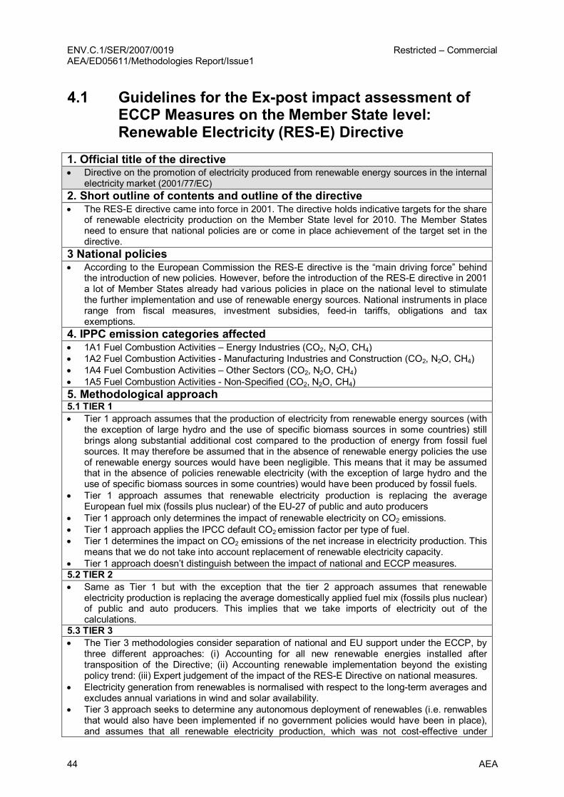
ENV.C.1/SER/2007/0019 Restricted – Commercial AEA/ED05611/Methodologies Report/Issue1
44 AEA
4.1 Guidelines for the Expost impact assessment of ECCP Measures on the Member State level: Renewable Electricity (RESE) Directive
1. Official title of the directive • Directive on the promotion of electricity produced from renewable energy sources in the internal
electricity market (2001/77/EC) 2. Short outline of contents and outline of the directive • The RESE directive came into force in 2001. The directive holds indicative targets for the share
of renewable electricity production on the Member State level for 2010. The Member States need to ensure that national policies are or come in place achievement of the target set in the directive.
3 National policies • According to the European Commission the RESE directive is the “main driving force” behind
the introduction of new policies. However, before the introduction of the RESE directive in 2001 a lot of Member States already had various policies in place on the national level to stimulate the further implementation and use of renewable energy sources. National instruments in place range from fiscal measures, investment subsidies, feedin tariffs, obligations and tax exemptions.
4. IPPC emission categories affected • 1A1 Fuel Combustion Activities – Energy Industries (CO2, N2O, CH4) • 1A2 Fuel Combustion Activities Manufacturing Industries and Construction (CO2, N2O, CH4) • 1A4 Fuel Combustion Activities – Other Sectors (CO2, N2O, CH4) • 1A5 Fuel Combustion Activities NonSpecified (CO2, N2O, CH4) 5. Methodological approach 5.1 TIER 1 • Tier 1 approach assumes that the production of electricity from renewable energy sources (with
the exception of large hydro and the use of specific biomass sources in some countries) still brings along substantial additional cost compared to the production of energy from fossil fuel sources. It may therefore be assumed that in the absence of renewable energy policies the use of renewable energy sources would have been negligible. This means that it may be assumed that in the absence of policies renewable electricity (with the exception of large hydro and the use of specific biomass sources in some countries) would have been produced by fossil fuels.
• Tier 1 approach assumes that renewable electricity production is replacing the average European fuel mix (fossils plus nuclear) of the EU27 of public and auto producers
• Tier 1 approach only determines the impact of renewable electricity on CO2 emissions. • Tier 1 approach applies the IPCC default CO2 emission factor per type of fuel. • Tier 1 determines the impact on CO2 emissions of the net increase in electricity production. This
means that we do not take into account replacement of renewable electricity capacity. • Tier 1 approach doesn’t distinguish between the impact of national and ECCP measures. 5.2 TIER 2 • Same as Tier 1 but with the exception that the tier 2 approach assumes that renewable
electricity production is replacing the average domestically applied fuel mix (fossils plus nuclear) of public and auto producers. This implies that we take imports of electricity out of the calculations.
5.3 TIER 3 • The Tier 3 methodologies consider separation of national and EU support under the ECCP, by
three different approaches: (i) Accounting for all new renewable energies installed after transposition of the Directive; (ii) Accounting renewable implementation beyond the existing policy trend: (iii) Expert judgement of the impact of the RESE Directive on national measures.
• Electricity generation from renewables is normalised with respect to the longterm averages and excludes annual variations in wind and solar availability.
• Tier 3 approach seeks to determine any autonomous deployment of renewables (i.e. renwables that would also have been implemented if no government policies would have been in place), and assumes that all renewable electricity production, which was not costeffective under
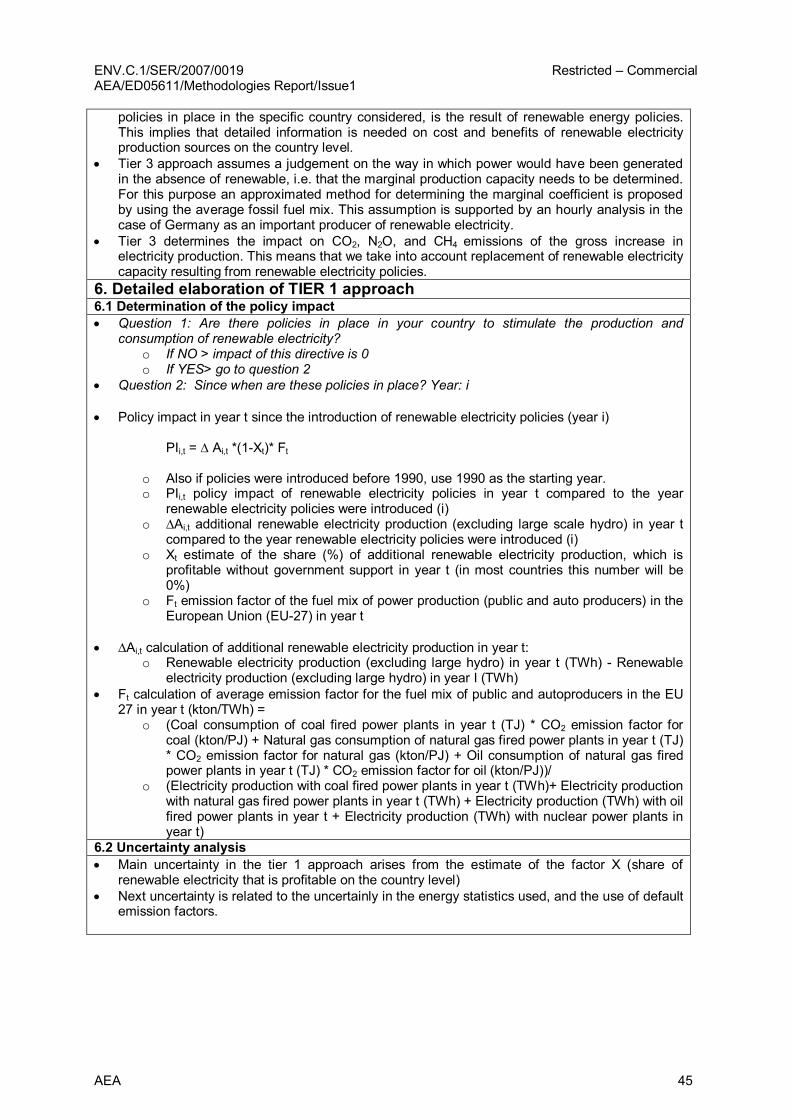
ENV.C.1/SER/2007/0019 Restricted – Commercial AEA/ED05611/Methodologies Report/Issue1
AEA 45
policies in place in the specific country considered, is the result of renewable energy policies. This implies that detailed information is needed on cost and benefits of renewable electricity production sources on the country level.
• Tier 3 approach assumes a judgement on the way in which power would have been generated in the absence of renewable, i.e. that the marginal production capacity needs to be determined. For this purpose an approximated method for determining the marginal coefficient is proposed by using the average fossil fuel mix. This assumption is supported by an hourly analysis in the case of Germany as an important producer of renewable electricity.
• Tier 3 determines the impact on CO2, N2O, and CH4 emissions of the gross increase in electricity production. This means that we take into account replacement of renewable electricity capacity resulting from renewable electricity policies.
6. Detailed elaboration of TIER 1 approach 6.1 Determination of the policy impact • Question 1: Are there policies in place in your country to stimulate the production and
consumption of renewable electricity? o If NO > impact of this directive is 0 o If YES> go to question 2
• Question 2: Since when are these policies in place? Year: i
• Policy impact in year t since the introduction of renewable electricity policies (year i)
PIi,t = ∆ Ai,t *(1Xt)* Ft
o Also if policies were introduced before 1990, use 1990 as the starting year. o PIi,t policy impact of renewable electricity policies in year t compared to the year
renewable electricity policies were introduced (i) o ∆Ai,t additional renewable electricity production (excluding large scale hydro) in year t
compared to the year renewable electricity policies were introduced (i) o Xt estimate of the share (%) of additional renewable electricity production, which is
profitable without government support in year t (in most countries this number will be 0%)
o Ft emission factor of the fuel mix of power production (public and auto producers) in the European Union (EU27) in year t
• ∆Ai,t calculation of additional renewable electricity production in year t: o Renewable electricity production (excluding large hydro) in year t (TWh) Renewable
electricity production (excluding large hydro) in year I (TWh) • Ft calculation of average emission factor for the fuel mix of public and autoproducers in the EU
27 in year t (kton/TWh) = o (Coal consumption of coal fired power plants in year t (TJ) * CO2 emission factor for
coal (kton/PJ) + Natural gas consumption of natural gas fired power plants in year t (TJ) * CO2 emission factor for natural gas (kton/PJ) + Oil consumption of natural gas fired power plants in year t (TJ) * CO2 emission factor for oil (kton/PJ))/
o (Electricity production with coal fired power plants in year t (TWh)+ Electricity production with natural gas fired power plants in year t (TWh) + Electricity production (TWh) with oil fired power plants in year t + Electricity production (TWh) with nuclear power plants in year t)
6.2 Uncertainty analysis • Main uncertainty in the tier 1 approach arises from the estimate of the factor X (share of
renewable electricity that is profitable on the country level) • Next uncertainty is related to the uncertainly in the energy statistics used, and the use of default
emission factors.

ENV.C.1/SER/2007/0019 Restricted – Commercial AEA/ED05611/Methodologies Report/Issue1
46 AEA
6.3 Data sources • Default emission factors for fossil fuel: http://www.ipcc
nggip.iges.or.jp/public/2006gl/pdf/2_Volume2/V2_2_Ch2_Stationary_Combustion.pdf (Table 2.2)
• Eurostat: Electricity generated from renewable energy sources • Eurostat: Electricity statistics • Eur’Observeur barometers for renewables 7. Issue to consider for future evaluations • Important for Tier 3 analysis is the development of a European model to capture the shortterm
RESEinduced changes (dispatching) in the power sector. The results of such a model need to be tested against simplified approximation methods for more EU countries (currently Germany was tested as a main producer of renewable electricity). In addition, one should develop more sophisticated approximation methods to "imitate" detailed power market modelling by econometric approaches.
• Rising electricity prices. If in future years the price of electricity will further increase, renewable electricity will benefits from this as it will become more competitive. This means that large part of renewable electricity production can be considered autonomous. Currently this issue is only considered in the Tier 3 analysis. It may, however, also be included in the Tier 1/2 analysis in the future. The “autonomous growth” of renewable energy production could be determined by calculating which renewable energy technologies are competitive with actual observed energy prices on the country level. The data will require:
1. Actual investments data per renewable energy technology (from a large variety of sources)
2. Actual energy prices for the various target groups on the Member State Level. Source Eurostat.
• Overlap with EUETS. In future years the cap for installations under the EU emissions trading sector will become more stringent. This will have a positive impact on the deployment of renewables as renewable electricity production will become more competitive. The overlap with the EU ETS is, however, an issue to be considered in the Tier 3 approach only.

ENV.C.1/SER/2007/0019 Restricted – Commercial AEA/ED05611/Methodologies Report/Issue1
AEA 47
4.2 Guidelines for the Expost impact assessment of ECCP Measures on the Member State level: Biofuels Directive
1. Official title of the directive • Directive on the promotion of the use of biofuels or other renewable fuels for transport
(2003/30/EC) and for future evaluation revised renewables Directive from 2008/2009. 2. Short outline of contents and outline of the directive • Member States were required to bring the Biofuels Directive into force by 31 December 2004.
Member States should ensure that a minimum proportion of biofuels and other renewable fuels is placed on their markets, and, to that effect, shall set national indicative targets. A reference value for these targets is 2 % on the basis of energy content, of all petrol and diesel for transport purposes placed on their markets by 31 December 2005, and 5.75% by 2010. The new Directive on Renewables from 2008 sets a 10% target for 2020. 14
3 National policies • Member States have various policies in place to achieve the targets set in the directive. Most
important instruments to stimulate demand for biofuels are obligations for blending fossil fuels and tax exemptions for biofuels.
4. IPPC emission categories affected • 1A3B Road Transport – passenger cars and goods transport (CO2, CH4, N2O)) • 3B Land (CH4, N2O) • 3C Aggregate Sources and NonCO2 Emissions Sources on Land (CH4, N2O) 5. Methodological approach • The shift from fossil transport fuels to biofuels reduces the emission of CO2 emissions from the
transport sector, but on the other hand can have an adverse effect on the emission of CH4 and N2O compared to fossil fuel use due to land use changes and cultivation. This can even lead the situation when looking at the total life cycle of biofuels no greenhouse gas reductions are achieved or even an increase of LCA is observed.
• National biofuel policies directly affect the CO2 emissions from the transport sector (emission category 1A3B), but the adverse impact on emission of CH4 and N2O can take place in another country. This means that they can not in all cases directly linked to the emission inventories of a specific country.
• As life cycle emission from biofuels is a crucial issue in the current discussion on the sustainability we have included them in the tier 1, 2 and 3 approach. However issues concerning landuse change can only be handled at the Tier 3 level, since there are no readily available and commonly agreed default emission factors.
5.1 TIER 1 • Tier 1 approach assumes that the consumption and production of biofuels still brings along
substantial additional cost compared to fossil transport fuels. It may therefore be assumed that in the absence of biofuel policies the use of biofuels would have been negligible. This means that it may be assumed that in the absence of policies only fossil transport fuels would have been produced and consumed.
• Tier 1 takes into account greenhouse gas emission over the lifetime of national biofuel consumption, and compares these to the lifecycle emission of fossil transport fuels.
• Tier 1 only distinguishes between the consumption of biodiesel and bioethanol. • Tier 1 applies default life cycle emission factors for biodiesel and bioethanol. This means that
we take a conservative average emission factor for Europe, and don’t look into the specific with respect to place of origin and production method of the consumed biofuels on the national level.
Default LCA greenhouse gas emissions (gCO2eq/MJ) Biodiesel 40.8 (average savings 47%) Bioethanol 51 (average savings 35%)
14 It should be noted that the Commission’s directive on the promotion of the use of energy from renewable sources (2008) sets targets on the basis of volume. Future evaluations should be sensitive to the potential need to convert volume to energy content.
ENV.C.1/SER/2007/0019 Restricted – Commercial AEA/ED05611/Methodologies Report/Issue1
48 AEA
Default LCA greenhouse gas emissions (gCO2eq/MJ) Diesel 86.2 Petrol 85
• Tier 1 approach applies the IPCC default CO2 emission factor per type of transport fuel.
5.2 TIER 2 • The tier 2 approach includes a further detailing of the biofuel categories on the level of the new
proposed directive on the promotion of the use of energy from renewable sources. • The tier 2 approach applies the default life cycle greenhouse gas emissions published in the
new proposed directive on the promotion of the use of energy from renewable sources.
5.3 TIER 3 • The tier 3 approach includes a further detailing of the biofuels down to the level that for each
individual stream the life cycle emission can be determined. This requires very detailed information on all produced and imported biofuels. It explores further the issue of direct and indirect landuse change and the impacts on default emission factors.
6. Detailed elaboration of TIER 1 approach 6.1 Determination of the policy impact • Question 1: Are there policies in place in your country to stimulate the production and
consumption of biofuels? o If NO > impact of this directive is 0 o If YES> go to question 2
• Question 2: Since when are these policies in place? Year: i
• Policy impact in year t since the introduction of biofuel policies (year i)
PIi,t = ADi,t * (EDFdefault EDBdefault) + APi,t * (EPFdefault
EPBdefault)
o Also if policies were introduced before 2003, use 2003 as the starting year. o PIi,t policy impact of biofuel policies in year t compared to the year biofuel policies were
introduced (i) o ∆ADi,t additional biodiesel production in year t compared to the year biofuel policies
were introduced (i) o EDFt default greenhouse gas life cycle emission factor for diesel o EDBt default greenhouse gas life cycle emission factor for biodiesel o ∆APi,t additional bioethanol production in year t compared to the year biofuel policies
were introduced (i) o EPFt default greenhouse gas life cycle emission factor for gasoline o EPBt default greenhouse gas life cycle emission factor for bioethanol
6.2 Uncertainty analysis • Main uncertainty in the tier 1 approach arises from application of the default life cycle emission
factors for biofuels • Next uncertainty is related to the uncertainly in the statistics on the consumption and production
of biofuels and missing information on the details of the feedstocks, especially also from imported biofuels
6.3 Data sources • Eurostat data on biofuels • Eurobserver: sales of biofuels http://www.energiesrenouvelables.org/observ
er/stat_baro/barobilan/barobilan7.pdf

ENV.C.1/SER/2007/0019 Restricted – Commercial AEA/ED05611/Methodologies Report/Issue1
AEA 49
7. Issue to consider for future evaluations • Inclusion of default emission factors from direct/indirect landuse change, as they emerge • Boundaries of the emission inventories (emissions may be increased outside the transport
sector). • As developments in this sector more very quickly, default factor for the tier 1 approach need to
be updated on a regular basis. • Rising energy prices. If in future years the price of oil will further increase, biofuels will benefits
from this as they will become more competitive. • Technological development. Innovations and further increase in production scale will probably
reduce cost of biofuel and making them more competitive. • Potential overlap with CAP policies should be further considered.
ENV.C.1/SER/2007/0019 Restricted – Commercial AEA/ED05611/Methodologies Report/Issue1
50 AEA
4.3 Guidelines for the Expost impact assessment of ECCP Measures on the Member State level: CHP Directive
1. Official title of the directive • Directive on the promotion of cogeneration based on a useful heat demand in the internal
electricity market (2004/8/EC) 2. Short outline of contents and outline of the directive • The CHP directive came into force in 2004. The purpose of the directive is to increase energy
efficiency and security of supply by creating a framework for promotion and development of high efficiency cogeneration. The directive obliges Member States 1) to set up a system for guarantees of origin for high efficiency cogeneration, 2) to establish an analysis of the national potential for high efficiency cogeneration including an analysis of barriers, 3) to ensure that support for cogeneration is based on useful heat demand and primary energy savings and 4) to evaluate the existing legislative and regulatory framework.
• All Member States have implemented the Directive into national legislation. This does however not mean that the Directive is (currently) fully operational at Member State level: • The guidelines for calculating electricity from cogeneration are not yet finalised. A
Commission Decision is expected end of 2008. • The systems for GOs for highefficiency cogeneration are not yet operational (waiting for the
Commission Decision on the calculation guidelines). • Only a number of Member States have submitted their national potential studies and progress
reports. The Commission has not yet evaluated the studies. • Only a number of Member States have adapted their national support schemes (use of
reference values, 10% primary energy threshold) but full adaptation is only possible when the calculation guidelines are ready.
The above means that the CHP Directive is unlikely to lead to a direct impact (over and above national policies) until at least 2009 i.e. the impact of the policy to date is zero.
2.1 Relevant reporting requirements under the Directive • Member States need to evaluate progress towards increasing the share of highefficiency
cogeneration every four years (first time not later than 21 February 2007) on request by the commission. In addition, Member States are required to submit annual statistics on national electricity and heat production from cogeneration as well as cogeneration capacities and fuels used. The Directive then requires the Commission to produce a report assessing Member State progress towards national targets every four years, starting in 2008.
3. Policy Interaction
EU Policies
The CHP Directive interacts with a widerange of other ECCP policies including EUETS, EPBD, RES H, and IPPCD. As CHP provides a more efficient option for heat and power generation, it can aid compliance with the various policies’ objectives. Hence policies such as the EUETS provide additional incentives for CHP deployment alongside those from the CHP Directive itself. National Policies • National instruments in place range from fiscal measures, investment subsidies, feedin
tariffs/premiums, obligations and tax exemptions. Most Member States already had CHP policies in place before the introduction of the directive.
4. IPPC emission categories affected • 1A1 Fuel Combustion Activities – Energy Industries (CO2, N2O, CH4) • 1A2 Fuel Combustion Activities Manufacturing Industries and Construction (CO2, N2O, CH4) • 1A4 Fuel Combustion Activities – Other Sectors (CO2, N2O, CH4) • 1A5 Fuel Combustion Activities NonSpecified (CO2, N2O, CH4) 5. Methodological approach 5.1 TIER 1 Tier 1 analysis for CHP is not to be considered a policy impact assessment. It shows the contribution
ENV.C.1/SER/2007/0019 Restricted – Commercial AEA/ED05611/Methodologies Report/Issue1
AEA 51
of CHP to climate policy objectives regardless whether this contribution is policy induced or not. Policy impacts can only be assessed with Tier 2 and 3 analyses. The Tier 1 methodology is based on Eurostat CHP statistics and composed of four steps: 1. For Tier 1 analysis 2004 is taken as the starting year, as this is the first year for which statistical
data for cogeneration is available for all Member States from Eurostat. 2. Secondly, when only total fuel (CHP fuel and nonCHP fuel) is available in the Eurostat CHP data
from a Member State, in Tier 1 the amount of CHP fuel is estimated. 3. Thirdly, the emission factor for electricity and heat which is being replaced by CHP is determined. 4. Finally, in Tier 1 the additional CO2 reduction from CHP is calculated
Appendix A provides a detailed description of the methodologies described above and details of the calculations performed can be found in appendix B. 5.2 TIER 2 • Tier 2 would allow a first order policy impact assessment • Tier 2 aims to increase the detail of the data which is used in the analysis.
o Identify all relevant sectors o Provides a first order estimate of autonomous deployment of CHP based on the growth of
the heat demand at sectoral level o Identify input (split into relevant fuel categories) and output data for different CHP
technologies at sectoral level o Identify each type of CHP technology the power capacity and number of installations at
sectoral level. • Tier 2 aims to identify the uptake of new CHP technologies such as microCHP, smallscale
biomass and fuel cell CHP • The Tier 2 analysis would calculate the emission factors for electricity and heat in the same
manner as per Tier 1, but using average Member State figures. 5.3 TIER 3 • Tier 3 analysis would allow a full policy impact assessment. • Tier 3 approach seeks to determine any autonomous deployment of CHP (i.e. CHP that would
also have been implemented if no government policies would have been in place), and assumes that all CHP electricity and heat production, which would not have been costeffective without policies in place in the specific Member State considered, is the result of CHP policies.
• Tier 3 approach seeks to determine the impact of operational support (feedin tariffs) to CHP and needs to assess how much CHP production would have fall back without the support.
• Tier 3 seeks to determine the interaction with the emissions trading directive and other ECCP policies.
• Tier 3 seeks to decompose the policy impact into impact from national policies and impact from the CHP Directive
• The Tier 3 emissions factors could be calculated by a variety of alternative approaches (see Appendix I for more details)
6. Issue to consider for future evaluations • Availability of CHP statistics – see Annex A below • Analysis of profitability of CHP is probably needed to improve the estimates in the reference
scenario. • When electricity prices grow more rapidly than fuel prices (improved spark spread) CHP will
become more competitive with the separate production of heat and electricity from fossil fuel sources. Some CHP will be profitable without government polices.
• Overlap with EUETS, EPBD, RESE/RES, IPPC, LCPD, Energy Services. § The future tightening of the emission cap for installations under the EU ETS will have an
effect on profitability of CHP. This will require simultaneously analysing the impact of the EU ETS and CHP Directive

ENV.C.1/SER/2007/0019 Restricted – Commercial AEA/ED05611/Methodologies Report/Issue1
52 AEA
Annex A: Explanations for main methodological assumptions
Determination of the policy impact since the introduction of the directive 1. For Tier 1 analysis 2004 is taken as the starting year, as this is the first year for which
statistical data for cogeneration is available for all Member States from Eurostat 15 . This is due to the reporting requirements in the Directive, which prescribe a split in reporting of CHP and nonCHP electricity from 2003 16 . All new/additional CHP from public producers assumed to be a result of 'policy'. Autogenerator CHP development assumed to be autonomous. However, Eurostat data does not fully split public / autoproducer electricity and heat production for all countries.
2. Secondly, when only total fuel (CHP fuel and nonCHP fuel) is available in the Eurostat CHP data from a Member State, in Tier 1 the amount of CHP fuel is estimated assuming a, relatively conservative, overall CHP efficiency of 75% 17 . Currently Eurostat only reports total fuel, but calculation guidelines from the Commission due to be adopted later in 2008 should mean that future statistics report this split.
3. Thirdly, the emission factor for electricity and heat which is being replaced by CHP is determined. The Tier 1 approach assumes that CHP electricity production is replacing the average fuel mix of the EU27 for fossil fired and nuclear public producers. The Tier 1 approach assumes that CHP heat is replacing the marginal factor associated with heat from a natural gasfired boiler with an efficiency of 85%.
4. Finally, in Tier 1 the additional CO2 reduction from CHP is calculated by the following formula: (CHP electricity (target year) x reference emission factor electricity (target year) + CHP heat (target year) / 85% x 56.8 kg CO2/GJ –CHP fuel (target year) x 56.8 kg CO2/GJ) (CHP electricity (2004) x reference emission factor electricity (2004) + CHP heat (2004) / 85% x 56.8 kg CO2/GJ –CHP fuel (2004) x 56.8 kg CO2/GJ).
In the formula it has been assumed that all CHP is natural gasfired. This assumption has been made due to a lack of statistical data on CHP fuels (only total fuel is available). Uncertainties • Various issues to do with existing data on CHP production, fuel use, etc. • Assumptions on standard factors for CHP/boiler efficiency. Data sources • Default emission factors for fossil fuel: http://www.ipcc
nggip.iges.or.jp/public/2006gl/pdf/2_Volume2/V2_2_Ch2_Stationary_Combustion.pdf (Table 2.2)
• Eurostat: CHP statistics 20042006
15 This differs from the general approach to evaluation where 1990 is taken as the starting year and the impact of a Directive is analysed relative to a continued trend from 1990 to the data of implementation of the Directive. 16 2004 has been taken as starting year since 2003 data are not available within Eurostat. 17 Currently, only in the Eurostat statistics for the UK the fuel has been split in CHP fuel and nonCHP fuel. It can be easily determined whether statistical data on fuels includes all fuel or CHP fuel only. When only CHP fuel is included the overall efficiency (sum of heat and electricity divided by fuel) is between 75 and 85% (or even higher). In case all fuel is included the overall efficiency is (far) below 75%.
ENV.C.1/SER/2007/0019 Restricted – Commercial AEA/ED05611/Methodologies Report/Issue1
AEA 53
Annex B: Detailed calculations for TIER 1
(Tier 2 and 3 calculations have not been considered for CHP)
Policy impact since introduction of the directive Step 1: see Annex A
Step 2: calculation of CHP fuel from total fuel • Overall CHP efficiency = 75% (assumption) • Overall CHP efficiency = (CHP heat + CHP electricity) / CHP fuel • Estimation of CHP fuel is therefore: (CHP heat + CHP electricity) / 75%
Step 3: see Annex A
Step 4: calculation of the additional CO2 reduction from CHP (CHP electricity (target year) x reference emission factor electricity (target year) + CHP heat (target year) / 85% x 56.8 kg CO2/GJ – CHP fuel (target year) x 56.8 kg CO2/GJ) (CHP electricity (2004) x reference emission factor electricity (2004) + CHP heat (2004) / 85% x 56.8 kg CO2/GJ –CHP fuel (2004) x 56.8 kg CO2/GJ).
When the total CO2 reduction from CHP is calculated, only the first part of the formula should be used: (CHP electricity (target year) x reference emission factor electricity (target year) + CHP heat (target year) / 85% x 56.8 kg CO2/GJ –CHP fuel (target year) x 56.8 kg CO2/GJ)
ENV.C.1/SER/2007/0019 Restricted – Commercial AEA/ED05611/Methodologies Report/Issue1
54 AEA
4.4 Guidelines for the Expost impact assessment of ECCP Measures on the Member State level: Voluntary Agreements for Cars between the European Commission and ACEA, JAMA and KAMA
4.4.1 Official title of the directive • Voluntary Agreements for Cars between the European Commission and ACEA, JAMA and KAMA 4.4.2 Short outline of contents and outline of the directive • The European Commission secured voluntary commitments with European (ACEA), Japanese
(JAMA) and Korean (KAMA) car manufacturers associations. The three Commitments contain the same quantified CO2 emission objective for the average of new passenger cars sold in the European Union, i.e. 140 gCO2/km (to be achieved by 2009 by JAMA and KAMA and by 2008 by ACEA). The commitments can be classed as a supplyside policy but are enhanced in some Member States by the introduction of financial incentives to stimulate the purchase of more energy efficient cars, as well as by the CO2/fuel efficiency labelling requirements (required by Directive 1999/94/EC).
• Between 1995 and 2004, CO2 emissions from road transport increased by 15% in the EU15. Between 1995 and 2004, however, the specific CO2 emissions of new passenger cars fell by 13% from 185 gCO2/km to 160 gCO2/km (EC, 2006) 18 . This improvement in CO2 emissions per km for new passenger cars could be the result of three factors: § policy impact: the agreement between the European Commission and the auto industry or
national demandside policies § the increasing share of diesel cars which are on average more efficient than petrolfuelled cars
(although increased dieselisation has been considered to be a consequence of the voluntary commitments, see section 5 below)
§ autonomous efficiency improvement • Even though not implemented until 1999, the commitments were being negotiated from 1995
onwards (thus potentially having an announcement effect on manufacturers) and manufacturers were aware of impending CO2 legislative pressure from 1992 (Ryan et al.). The period of policy impact proposed is therefore 1995 to the latest year for which data is available.
Relevant reporting requirements under the Directive
Monitoring and reporting of progress by Member States is a requirement of the Community’s strategy to reduce emissions of CO2 from new passenger cars (COM(95)689). Decision 1753/2000/EC establishing a scheme to monitor the average specific emissions of carbon dioxide from new passenger cars required that in the intermediate target year of 2003, a review was conducted that aimed to “…indicate whether the reduction achieved were due to technical measurers taken by the manufacturers of to other measures such as changes in consumer behaviour…”. Additionally, the relevant car manufacturers were obliged to carry out a joint “Major Review” based on 2003 data.
18 EC (2006). Implementing the Community Strategy to Reduce CO2 Emissions from Cars: Sixth Annual Communication on the effectiveness of the strategy. COM(2006) 463 final, European Commission, Brussels.
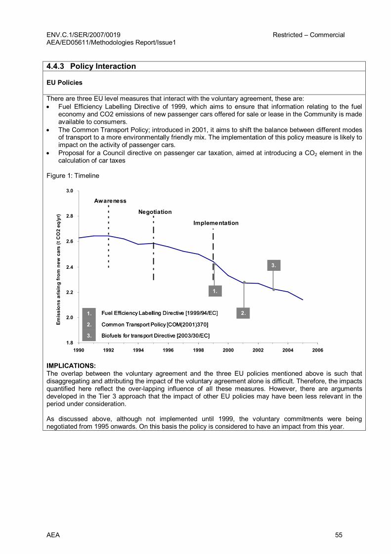
ENV.C.1/SER/2007/0019 Restricted – Commercial AEA/ED05611/Methodologies Report/Issue1
AEA 55
4.4.3 Policy Interaction
EU Policies
There are three EU level measures that interact with the voluntary agreement, these are: • Fuel Efficiency Labelling Directive of 1999, which aims to ensure that information relating to the fuel
economy and CO2 emissions of new passenger cars offered for sale or lease in the Community is made available to consumers.
• The Common Transport Policy; introduced in 2001, it aims to shift the balance between different modes of transport to a more environmentally friendly mix. The implementation of this policy measure is likely to impact on the activity of passenger cars.
• Proposal for a Council directive on passenger car taxation, aimed at introducing a CO2 element in the calculation of car taxes
Figure 1: Timeline
1.8
2.0
2.2
2.4
2.6
2.8
3.0
1990 1992 1994 1996 1998 2000 2002 2004 2006
Emission
s arising from
new
cars (t CO2 eq
/yr)
Awareness
Negotiation
Implementation
2.
3.
1.
1.
2.
3.
Fuel Efficiency Labelling Directive [1999/94/EC]
Common Transport Policy [COM(2001)370]
Biofuels for transport Directive [2003/30/EC] 1.8
2.0
2.2
2.4
2.6
2.8
3.0
1990 1992 1994 1996 1998 2000 2002 2004 2006
Emission
s arising from
new
cars (t CO2 eq
/yr)
Awareness
Negotiation
Implementation
2.
3.
1.
1.
2.
3.
Fuel Efficiency Labelling Directive [1999/94/EC]
Common Transport Policy [COM(2001)370]
Biofuels for transport Directive [2003/30/EC]
1.
2.
3.
Fuel Efficiency Labelling Directive [1999/94/EC]
Common Transport Policy [COM(2001)370]
Biofuels for transport Directive [2003/30/EC]
IMPLICATIONS: The overlap between the voluntary agreement and the three EU policies mentioned above is such that disaggregating and attributing the impact of the voluntary agreement alone is difficult. Therefore, the impacts quantified here reflect the overlapping influence of all these measures. However, there are arguments developed in the Tier 3 approach that the impact of other EU policies may have been less relevant in the period under consideration.
As discussed above, although not implemented until 1999, the voluntary commitments were being negotiated from 1995 onwards. On this basis the policy is considered to have an impact from this year.
ENV.C.1/SER/2007/0019 Restricted – Commercial AEA/ED05611/Methodologies Report/Issue1
56 AEA
National Policies
• According to the IEA’ s database of climate change policies and measures, prior to negotiations of the voluntary agreement there was only one national policy in place that interacts with the voluntary agreement 19 .
• Following the implementation of the voluntary agreement, around 26 policies have been introduced at the MS level that could impact emissions from passenger cars. It is likely that many of these measures can be linked to the EU legislation discussed earlier, however it should be recognised that the greenhouse gas impacts calculated for the voluntary agreement will, to some extent, reflect national policies independent of EU legislation.
4.4.4 IPCC emission categories affected • IPCC category 1A3b Road Transportation (policy only affects emissions from new passenger cars) • CO2, N20, CH4
4.4.5 Methodological approach
TIER 1
Assessment of the policy impact over the period since the voluntary agreement was implemented is based on the following:
• Emission rate of new vehicles (g CO2/km) are EU averages • The upper bound of the policy impact is estimated from the time series of: emission rates of new
cars; number of new registrations; and, average distance travelled per passenger car. Counterfactual scenario: In the absence of the voluntary agreement, it is assumed that new passenger car efficiencies would have remained at the 1995 level.
Appendix A provides a detailed description of the methodologies described above and details of the calculations performed can be found in appendix B.
TIER 2
The following adjustments are made in the Tier 2 approach: • National data for emission rate of new vehicles (g CO2/km) substitutes EU averages • Hidden structural effects relating to the shift from petrol to diesel fuel are calculated and its affects
isolated from the policy scenario. Counterfactual scenario: In the absence of the voluntary agreement, it is assumed that no passenger car efficiency improvements would have been made. However, the shift in new passenger cars towards diesels would have occurred. The correction due to autonomous dieselisation is 8% for the EU 15 20 .
19 Austria: Strategic plan to reduce transport’s CO2 emissions (1991) 20 It should be noted that the correction factor, which reflects the attribution of greenhouse gas reductions to dieselisation not the voluntary agreement, varies across MS. The value quoted here is calculated for EU 15 statistics and using the methodology discussed in Annex A and B
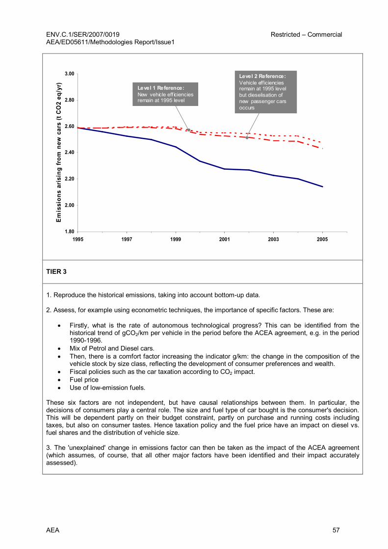
ENV.C.1/SER/2007/0019 Restricted – Commercial AEA/ED05611/Methodologies Report/Issue1
AEA 57
1.80
2.00
2.20
2.40
2.60
2.80
3.00
1995 1997 1999 2001 2003 2005
Emission
s arising from
new
cars (t CO2 eq
/yr) Level 1 Reference:
New vehicle eff iciencies remain at 1995 level
Level 2 Reference: Vehicle efficiencies remain at 1995 level but dieselisation of new passenger cars occurs
1.80
2.00
2.20
2.40
2.60
2.80
3.00
1995 1997 1999 2001 2003 2005
Emission
s arising from
new
cars (t CO2 eq
/yr) Level 1 Reference:
New vehicle eff iciencies remain at 1995 level
Level 2 Reference: Vehicle efficiencies remain at 1995 level but dieselisation of new passenger cars occurs
TIER 3
1. Reproduce the historical emissions, taking into account bottomup data.
2. Assess, for example using econometric techniques, the importance of specific factors. These are:
• Firstly, what is the rate of autonomous technological progress? This can be identified from the historical trend of gCO2/km per vehicle in the period before the ACEA agreement, e.g. in the period 19901996.
• Mix of Petrol and Diesel cars. • Then, there is a comfort factor increasing the indicator g/km: the change in the composition of the
vehicle stock by size class, reflecting the development of consumer preferences and wealth. • Fiscal policies such as the car taxation according to CO2 impact. • Fuel price • Use of lowemission fuels.
These six factors are not independent, but have causal relationships between them. In particular, the decisions of consumers play a central role. The size and fuel type of car bought is the consumer's decision. This will be dependent partly on their budget constraint, partly on purchase and running costs including taxes, but also on consumer tastes. Hence taxation policy and the fuel price have an impact on diesel vs. fuel shares and the distribution of vehicle size.
3. The 'unexplained' change in emissions factor can then be taken as the impact of the ACEA agreement (which assumes, of course, that all other major factors have been identified and their impact accurately assessed).

ENV.C.1/SER/2007/0019 Restricted – Commercial AEA/ED05611/Methodologies Report/Issue1
58 AEA
4.4.6 Issues to consider for future evaluations 1. The data basis for this analysis is sufficient. In the area of road vehicles, MS report detailed figures on numbers and types of cars sold and the emissions characteristics of each type under Decision 1753/2000/EC. 2. Exante evaluation of future policies must include a realistic appreciation of the trends in consumer preferences. Factors leading to the adoption of new technologies and alternative modes of transport need to be assessed.
3. It is not sufficient to analyse a single policy on its own. The effectiveness of a policy such as the ACEA is dependent on supporting measures such as fiscal incentives to buy more fuel efficient cars and information measures to ensure that information on fuel efficiency is readily available. Such an analysis may be carried out with transport models such as the ASTRA model used in this work in order to reflect well the interactions between different factors

ENV.C.1/SER/2007/0019 Restricted – Commercial AEA/ED05611/Methodologies Report/Issue1
AEA 59
4.4.7 Annex A: Explanations for main methodological assumptions
4.4.8 TIER 1
Determination of the policy impact since the voluntary agreement
At this stage, the voluntary agreement is assumed to be responsible for the full change in fuel economy of new passenger cars over the period. Autonomous improvements are not estimated, assuming that any improvements were counteracted by air quality and safety standards and changing consumer preferences for larger and heavier cars.
The calculations use the number of new registrations each year and the difference in the emission rate of those cars from the 1995 level. Combining this information with the average distance driven by cars within each year gives an estimate of the emissions that have been avoided due to increasing vehicle efficiency, relative to the base case in which emission rates remained at 1995 levels.
To estimate the upper bound for the impact of the change in fuel economy of passenger cars, the Tier 1 assessment, the following assumptions are applied:
• emissions from new cars would remain at 1995 levels in the absence of the policy • without the ACEA agreement the same number of new cars would have been introduced, but with
1995 emission rates • each year the most polluting cars (i.e. those from pre1995) are replaced by new passenger vehicles
(i.e. post1995 cars do not replace other post1995 cars) • all new vehicles introduced since 1995 are still in existence in the latest year • for an estimation of the impact in latest year, assume that cars from each year are driving same
2005 average kms • to estimate of impact over the period 19952005, assume that the new cars introduced each year
travel the average distance in that and each subsequent year
Uncertainty analysis:
Main uncertainty in the tier 1 approach arises from the assumption that emissions from new cars would remain at 1995 levels in the absence of the policy. In order to improve the analysis, the autonomous improvement of new passenger emission rates would need to be calculated. It would then be possible to refine the estimate of the impact of the voluntary agreement itself by attributing some of the efficiency improvements that would have occurred in the absence of the agreement.
Other uncertainties to be considered include: § Scrapping rate. The approach assumes that new registrations will only replace the oldest cars in
the vehicle fleet § The tier 1 analysis assumes that new cars drive the average vehicle kms calculated for the entire
passenger car fleet in a specific year. There is evidence that new cars would travel further than the average across the whole fleet.
§ The impact of increases in the mass of passenger cars on the autonomous efficiency improvement. It is anticipated that any general trend towards more efficient vehicles could have been offset, to a lesser or greater extent, by increases in average vehicle mass in the period since the agreement.
§ Rebound effects are not considered i.e. the financial savings from the improved fuel efficiency do not lead to increased mileage.
Data sources:
• ACEA (2006). European motor vehicle parc 2004, European Automobile Manufacturers Association, Brussels.
• EC (2006). Implementing the Community Strategy to Reduce CO2 Emissions from Cars: Sixth annual Communication on the effectiveness of the strategy. COM(2006) 463 final, European Commission, Brussels.
• ENERDATA s.a. (2008) WORLD ENERGY DATABASE
ENV.C.1/SER/2007/0019 Restricted – Commercial AEA/ED05611/Methodologies Report/Issue1
60 AEA
4.4.9 TIER 2
Over the past decade there has been growth in the number of diesel cars. Some analysts state that the voluntary agreements are responsible for some of the dieselisation, but not all as fuel taxes in many EU countries favour diesel over petrol – the UK is in a minority in that its taxes do not. Ricardo (2003) attribute all of the shift towards diesel car ownership to the voluntary agreement. However, here it is assumed that although the technical improvement in efficiency of diesels can be attributed to the VA (at this stage), the shift in ownership is caused by alternative influences. Therefore, this shift would have impacted on emissions from new vehicles even if the ACEA agreement had not been struck and it is necessary to estimate the impact on emissions from ‘autonomous dieselisation’.
The reported average petrol and diesel emission rates for newly registered cars in each year and the proportion of the new registration represented by petrol and diesel engines are used to generate average emission factors for newly registered vehicles in each year. Average emission factors are then calculated for each year since 1995 for a scenario in which the proportion of newly registered cars with petrol and diesel engines remains at 1995 levels. The difference between reported and ‘unshifted’ emission rates for newly registered cars, combined with the number of registrations in each year and the average distance driven by passenger cars in that year, provides an estimate of the emission change resulting from the shift in passenger car fleet composition from petrol towards diesel. This change is not attributed to the voluntary agreement and it has been removed from the upper bound calculated in the Tier 1 assessment.
In order to calculate the impact of dieselisation under the Level 2 assessment the following assumptions are applied: • In the absence of fuel specific emission rates, it is assumed that the diesel and petrol emission rates
follow the same trend as the overall change in the emission rate for new cars respectively • It is assumed that the diesel share of passenger vehicles is frozen at 1995 share
4.4.10 TIER 3 See the detailed report on the illustrative Tier 3 approach
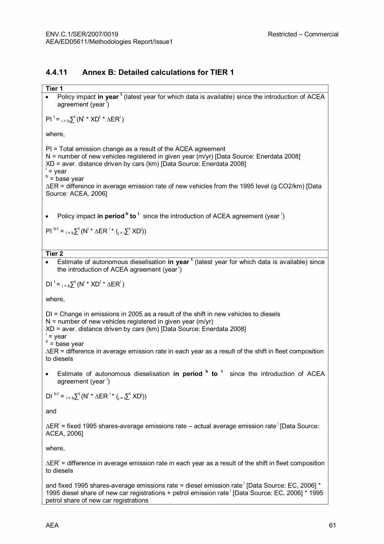
ENV.C.1/SER/2007/0019 Restricted – Commercial AEA/ED05611/Methodologies Report/Issue1
AEA 61
4.4.11 Annex B: Detailed calculations for TIER 1
Tier 1 • Policy impact in year t (latest year for which data is available) since the introduction of ACEA
agreement (year i )
PI t = i = b∑ t (N i * XD t * ∆ER i )
where,
PI = Total emission change as a result of the ACEA agreement N = number of new vehicles registered in given year (m/yr) [Data Source: Enerdata 2008] XD = aver. distance driven by cars (km) [Data Source: Enerdata 2008] i = year b = base year ∆ER = difference in average emission rate of new vehicles from the 1995 level (g CO2/km) [Data Source: ACEA, 2006]
• Policy impact in period b to t since the introduction of ACEA agreement (year i )
PI b:t = i = b∑ t (N i * ∆ER i * (j = i∑ t XD j ))
Tier 2 • Estimate of autonomous dieselisation in year t (latest year for which data is available) since
the introduction of ACEA agreement (year i )
DI t = i = b∑ t (N i * XD t * ∆ER i )
where,
DI = Change in emissions in 2005 as a result of the shift in new vehicles to diesels N = number of new vehicles registered in given year (m/yr) XD = aver. distance driven by cars (km) [Data Source: Enerdata 2008] i = year b = base year ∆ER = difference in average emission rate in each year as a result of the shift in fleet composition to diesels
• Estimate of autonomous dieselisation in period b to t since the introduction of ACEA agreement (year i )
DI b:t = i = b∑ t (N i * ∆ER i * (j = i∑ t XD j ))
and
∆ER i = fixed 1995 sharesaverage emissions rate – actual average emission rate i [Data Source: ACEA, 2006]
where,
∆ER i = difference in average emission rate in each year as a result of the shift in fleet composition to diesels
and fixed 1995 sharesaverage emissions rate = diesel emission rate i [Data Source: EC, 2006] * 1995 diesel share of new car registrations + petrol emission rate i [Data Source: EC, 2006] * 1995 petrol share of new car registrations

ENV.C.1/SER/2007/0019 Restricted – Commercial AEA/ED05611/Methodologies Report/Issue1
62 AEA
Tier 2 (possible additional improvement by introducing autonomous change) • Establishing a counterfactual (emissions that would have occurred in the absence of the
ACEA agreement) based on prepolicy implementation emission rates.
• Total change in emissions arising in 2005 as a result of autonomous change
AI t = i = b∑ t (N i * XD t * ∆ER i )
where,
AI = Total change in emissions arising in 2005 as a result of autonomous change N = number of new vehicles registered in given year (m/yr) [Data Source: Enerdata 2008] XD = aver. distance driven by cars (km) [Data Source: Enerdata 2008] i = year b = base year ∆ER = difference in average emission rate of new vehicles from the 1995 level (g CO2/km) [Data Source: ACEA, 2006]
• Total change in emissions arising over the period 1995 2005 as a result of autonomous change
PI b:t = i = b∑ t (N i * ∆ER i * (j = i∑ t XD j ))
And
∆ER i = emission rate of new cars i change in emission rate per year over the period 1980 – 1994 or another suitable period [Data Source: Enerdata 2008].

ENV.C.1/SER/2007/0019 Restricted – Commercial AEA/ED05611/Methodologies Report/Issue1
AEA 63
4.5 Guidelines for the Expost impact assessment of ECCP Measures on the Member State level: Landfill Directive
1. Official title of the directive • Directive on the landfill of waste 2. Short outline of contents and outline of the directive • The Landfill Directive sets out legislation for the reduction of Municipal Solid Waste disposed to
landfill and sets targets to reduce biodegradable waste to landfill progressively by 25%, 50%, 65% compared to 1995 levels.
• The deadline for implementation of the Landfill Directive (Directive 1999/31/EC) in the Member States was 16.07.2001. Its objective is to prevent or reduce as far as possible negative effects on the environment from the landfilling of waste, by introducing stringent technical requirements for waste and landfills. The Directive aims to achieve these objectives by inter alia: encouraging a reduction in the amount of municipal solid waste being landfilled through diversion to alternative processing techniques; and, encouraging recovery of gases produced at landfill sites. Within this project we are interested in the impact of the landfill directive on greenhouse gas emissions (i.e. CH4 and CO2).
• Objectives are established for the progressive reduction of biodegradable waste to landfill by 25% within five years of Member State implementation of the Directive, 50% within eight years, and by 65% within fifteen years, compared to 1995 levels.
Relevant reporting requirements under the Directive
The Directive requires Member States to report on the implementation in respect of their national strategies every three years. The Commission is then required to publish a Community report within 9 months of receiving the MS reports. 3. Policy Interaction
EU Policies
There are two EU level measures that interact with the Landfill Directive, these are: • Integrated Pollution Prevention and Control (IPPC) Directive, which lays down measures to
prevent or reduce emissions to the air, water and land from activities including waste management.
• Waste Incineration Directive (WID), which aims to regulate the incineration of hazardous waste in order to prevent excessive pollution to air, water and soil. WID applies to existing plants and new plants and requires all incineration and coincineration plants to be authorised, implement measurement and monitoring systems, and maximise energy recovery.
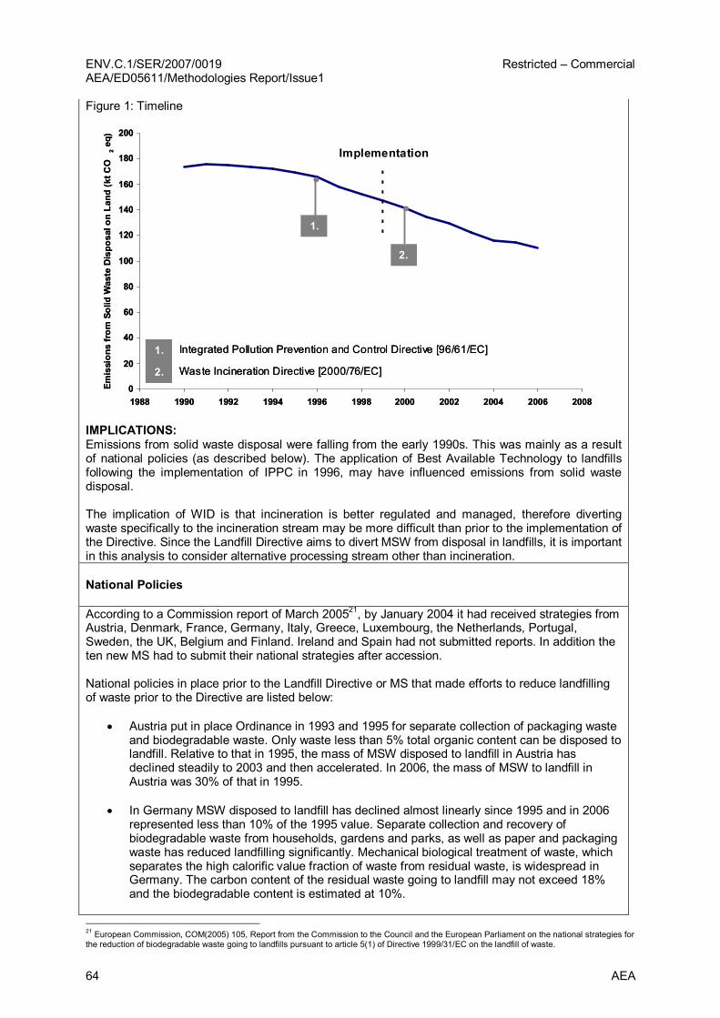
ENV.C.1/SER/2007/0019 Restricted – Commercial AEA/ED05611/Methodologies Report/Issue1
64 AEA
Figure 1: Timeline
0
20
40
60
80
100
120
140
160
180
200
1988 1990 1992 1994 1996 1998 2000 2002 2004 2006 2008
Emission
s from
Solid Waste Dispo
sal o
n La
nd (k
t CO
2 eq)
Implementation
1.
2.
1. Integrated Pollution Prevention and Control Directive [96/61/EC]
2. Waste Incineration Directive [2000/76/EC] 0
20
40
60
80
100
120
140
160
180
200
1988 1990 1992 1994 1996 1998 2000 2002 2004 2006 2008
Emission
s from
Solid Waste Dispo
sal o
n La
nd (k
t CO
2 eq)
Implementation
1.
2.
1. Integrated Pollution Prevention and Control Directive [96/61/EC] 1. Integrated Pollution Prevention and Control Directive [96/61/EC]
2. Waste Incineration Directive [2000/76/EC] 2. Waste Incineration Directive [2000/76/EC]
IMPLICATIONS: Emissions from solid waste disposal were falling from the early 1990s. This was mainly as a result of national policies (as described below). The application of Best Available Technology to landfills following the implementation of IPPC in 1996, may have influenced emissions from solid waste disposal.
The implication of WID is that incineration is better regulated and managed, therefore diverting waste specifically to the incineration stream may be more difficult than prior to the implementation of the Directive. Since the Landfill Directive aims to divert MSW from disposal in landfills, it is important in this analysis to consider alternative processing stream other than incineration.
National Policies
According to a Commission report of March 2005 21 , by January 2004 it had received strategies from Austria, Denmark, France, Germany, Italy, Greece, Luxembourg, the Netherlands, Portugal, Sweden, the UK, Belgium and Finland. Ireland and Spain had not submitted reports. In addition the ten new MS had to submit their national strategies after accession.
National policies in place prior to the Landfill Directive or MS that made efforts to reduce landfilling of waste prior to the Directive are listed below:
• Austria put in place Ordinance in 1993 and 1995 for separate collection of packaging waste and biodegradable waste. Only waste less than 5% total organic content can be disposed to landfill. Relative to that in 1995, the mass of MSW disposed to landfill in Austria has declined steadily to 2003 and then accelerated. In 2006, the mass of MSW to landfill in Austria was 30% of that in 1995.
• In Germany MSW disposed to landfill has declined almost linearly since 1995 and in 2006 represented less than 10% of the 1995 value. Separate collection and recovery of biodegradable waste from households, gardens and parks, as well as paper and packaging waste has reduced landfilling significantly. Mechanical biological treatment of waste, which separates the high calorific value fraction of waste from residual waste, is widespread in Germany. The carbon content of the residual waste going to landfill may not exceed 18% and the biodegradable content is estimated at 10%.
21 European Commission, COM(2005) 105, Report from the Commission to the Council and the European Parliament on the national strategies for the reduction of biodegradable waste going to landfills pursuant to article 5(1) of Directive 1999/31/EC on the landfill of waste.
ENV.C.1/SER/2007/0019 Restricted – Commercial AEA/ED05611/Methodologies Report/Issue1
AEA 65
• In Denmark, as of 1997 all municipalities have been obliged to send waste suitable for incineration to incineration, effectively banning the landfilling of combustible waste.
• France implemented an act of 13 July 1992, which required that by 1 July 2002 only waste that cannot be treated anymore under the present technical and economic conditions may be accepted by landfills.
• In Italy, an ecotax has been in place since 1995, which has been effective in reducing the amount of waste going to landfills.
• In the Netherlands, the 1997 decree on landfills and landfill bans prohibits the landfilling of separately collected vegetable, fruit and garden waste, waste of plant origin from agriculture and horticulture, market waste, waste from public parks and gardens or green waste from public spaces.
4. IPCC emission categories affected • IPCC category 6A Solid waste disposal on land, 6C Waste Incineration • CO2, CH4 and N2O (from waste recycling and biological waste treatment) 5. Methodological approach
TIER 1
The Tier 1 assessment of the policy impact of the Landfill Directive over the period since implementation focuses on CH4 emissions and is based on the methodology proposed in the IPCC guidance 22 for calculating CH4 emissions:
• A first order decay (FOD) model is used to describe the decomposition of organic matter in muncipal waste disposed to landfills.
• Default IPCC values are taken for the decay model, these include: waste composition; methane correction factor; degradable organic carbon fraction of waste; fraction of decomposable degradable organic matter (DDOC); fraction of CH4 in landfill gas; decay rate constants.
• The central assumption of the counterfactual for disposal of MSW to landfill is that in the absence of the Landfill Directive the fraction of MSW disposed to landfill would have remained at 1999 levels. Therefore the difference in waste disposed to landfill between this counterfactual and the reported masses can be assigned to the Directive. Accordingly, any CH4 emissions arising from this waste can also be assigned as savings brought about by the implementation of the Directive.
Appendix A provides a detailed description of the methodologies described above and details of the calculations performed can be found in appendix B.
TIER 2
The aim of the Tier 2 methodology is to attempt to rectify the main weaknesses of the Tier 1 methodology. Therefore, this level of analysis advances the complexity of the first order decay method used for Tier 1. Refinements made include the following:
1. An attempt is made to include autonomous changes in the mass of waste disposed to landfill, since for some MS there was a downward trend prior to the implementation of the Landfill Directive. The linear trend in waste seen for the years 1995 to 1998 is extrapolated through to the present as a counterfactual for waste disposed to landfill.
2. Where available, MS specific data is used for the FOD model parameters. 3. In addition to diverting waste from disposal in landfills, the Directive aims to increases the rates
of landfill gas recovery from waste sites. Therefore, the tier 2 analysis attempts to include the effects of the increased rate of recovery as a result of the Directive by assuming that in the absence of the Directive, recovery rates would have remained at 1999 levels. Therefore, the emissions associated with the difference in emissions can be assigned as a saving resulting from the implementation of the Landfill Directive.
22 IPCC, 2006, Guidelines for National Greenhouse Gas Inventories
ENV.C.1/SER/2007/0019 Restricted – Commercial AEA/ED05611/Methodologies Report/Issue1
66 AEA
4. Given that waste diverted away from landfill is processed by another technology, the emissions associated with those processes should be calculated and removed from the impact of the Directive. Here we calculated the emissions associated with increased recycling and biological treatment. In order to calculate these emissions, it is assumed that in the absence of the Directive the fraction of waste passing through these streams would have remained at 1999 levels. In a similar way we calculate the emissions associated with increased incineration, however, we also consider the emissions avoided as a result of energy displaced by energy recovered from the incineration process. This is distinct from the WID analysis since it considers only the impacts of the change in mass of waste disposed through waste incineration but does not consider the changes in energy recovered from the incineration process, which is the focus of the analysis of the Waste Incineration Directive.
TIER 3
The principal development for a Tier 3 analysis would be to refine the counterfactual for waste disposed through the various processing streams in the absence of the Directive.
The EEA have recently carried out a modelling exercise for projecting greenhouse emissions arising from the waste sector in Europe. As a part of this exercise, they calculated models for total MSW generation, however, the fraction of this waste disposed to landfill was based on best estimates. It would be beneficial to consider if a model for mass of waste disposed to landfill could be developed based on data on landfill rates over the period prior to the implementation of the Landfill Directive. 6. Issues to consider for future evaluations • Reported recovery rates of landfill gas from landfill sites are under debate. Some MS report
near or complete recovery. However, the recent IPCC guidance takes issue with this level of recovery and recommends that for reporting an upper limit of 20% is used. For the current assessment the reported recovery rates are used, however, this should be reviewed for any further assessment.
• The definition of MSW varies between MS. To inform the evaluation of the impact of the Landfill Directive, reporting on the sources of waste would be useful.
• The analysis proposed here does not rely on UNFCCC reported emission or activity data since there may be a discrepancy between the definition of solid waste disposed to landfill (emission sector 6.A) and that of Landfill Directive compliant sites.
Annex A: Explanations for main methodological assumptions
TIER 1
Determination of the policy impact since the Landfill Directive
A first order decay (FOD) model for the decay of degradable organic matter in landfills is used to predict the emissions associated with the MSW that would have been disposed to landfill in the absence of the Landfill Directive. The assumption is made that in the absence of the Directive, the proportion of generated MSW disposed to landfill would remain at 2001 levels.
Emissions are calculated for the decay of at least 98% the waste (more for the faster decaying components of the waste).
The parameters used in the FOD model are taken as the IPCC default values, which are specific to Northern, Eastern, Southern and Western Europe.
Uncertainty analysis:
The main uncertainty in the tier 1 approach arises from the assumption that the proportion of the mass of MSW generated that is disposed of to landfill and its emission rate would remain at 2001

ENV.C.1/SER/2007/0019 Restricted – Commercial AEA/ED05611/Methodologies Report/Issue1
AEA 67
levels in the absence of the policy.
Data sources:
• Eurostat: Municipal Solid Waste disposed to landfill per capita; Population. • EEA, 2008, Municipal waste management and greenhouse gases: fraction of MSW disposed to
landfill. • IPCC, 2006, Guidelines for National Greenhouse Gas Inventories: default values for waste
composition, methane correction factor, degradable organic carbon fraction of waste, fraction of decomposable degradable organic matter (DDOC), fraction of CH4 in landfill gas, decay rate constants.
TIER 2
Determination of the policy Impact since the Landfill Directive
Refining the Tier 1 methodology, this level of analysis considers: • Autonomous change. A linear regression of the fraction of MSW disposed to landfill against time
prior to the implementation of the Directive is carried out and used to extrapolate the trend as a counterfactual for the absence of the Directive.
• MS Specific data used for the FOD parameters. The recommendation will be made that where available MS specific data should be used. For our analysis the only MS specific data available that could be included was the composition of MSW.
• Recovery rates based on the recovered emissions reported to the UNFCCC were used to consider how the Landfill Directive has influenced the capture and use of landfill gas. The impact of the Directive on recovery of gas was calculated by assuming that in the absence of the Directive the percentage of emissions recovered would remain at 2001 levels.
• Emissions arising from waste diverted to recycling and biological treatment. It is assumed that the waste not disposed by landfilling or incineration is split 50:50 between recycling and mechanical treatment. Additionally, emissions are calculated for the waste diverted to incineration and for the emissions avoided through use of energy recovered from the incineration process.
Uncertainty analysis
The principal uncertainties for this analysis are the counterfactuals in the absence of the Directive for: 1. Mass of waste disposed to landfill. 2. Recovery rate 3. Incineration rate 4. Recycling rate 5. Biological treatment rate.
Data sources
• Eurostat: Municipal Solid Waste disposed to landfill per capita; Population. • EEA, 2008, Municipal waste management and greenhouse gases: fraction of MSW disposed to
landfill. • IPCC, 2006, Guidelines for National Greenhouse Gas Inventories: methane correction factor,
degradable organic carbon fraction of waste, fraction of decomposable degradable organic matter (DDOC), fraction of CH4 in landfill gas, decay rate constants, emission factors for biological processing.
• EEA, 2008, Municipal waste management and greenhouse gases: MS specific waste composition, Fraction of waste incinerated, Emission factors for incineration and recycling.
• UNFCCC, CRF tables: Landfill gas recovery rates.
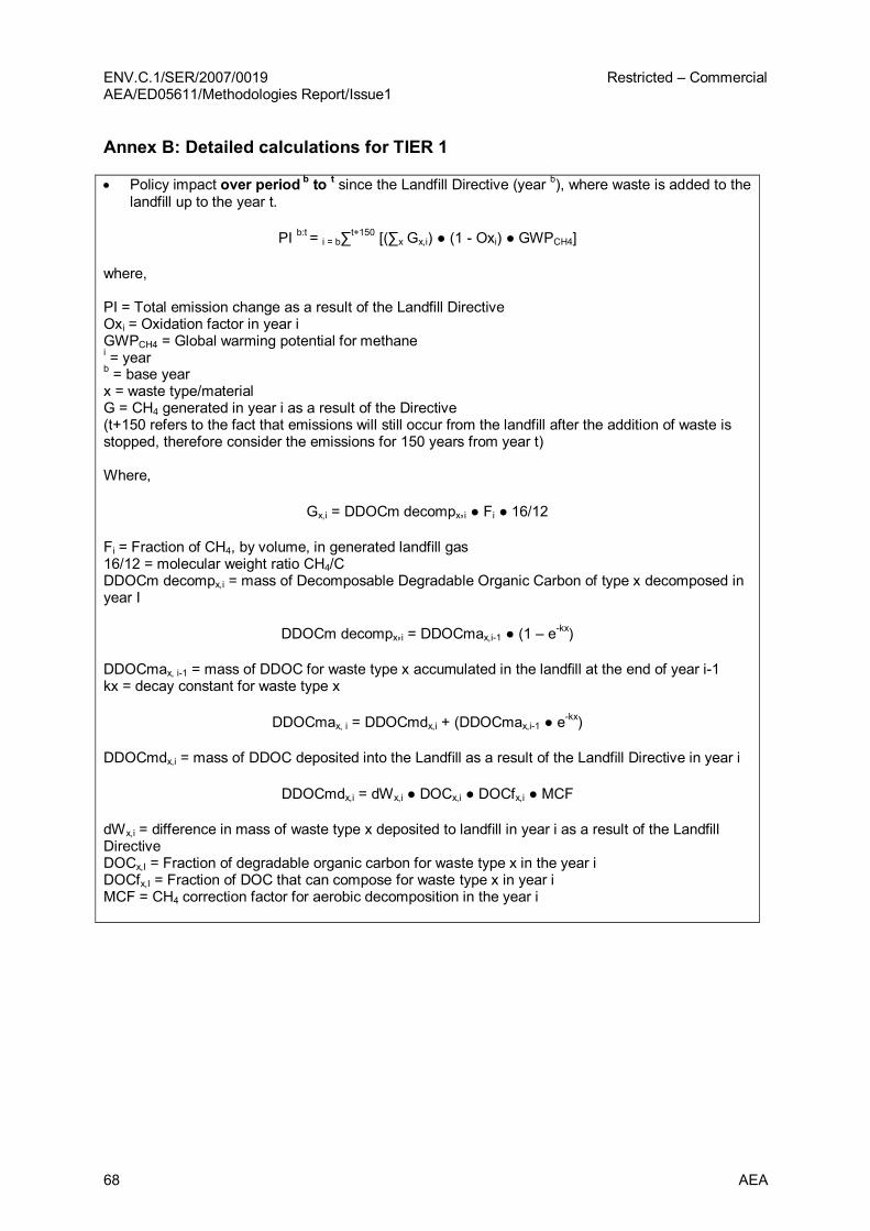
ENV.C.1/SER/2007/0019 Restricted – Commercial AEA/ED05611/Methodologies Report/Issue1
68 AEA
Annex B: Detailed calculations for TIER 1
• Policy impact over period b to t since the Landfill Directive (year b ), where waste is added to the landfill up to the year t.
PI b:t = i = b∑ t+150 [(∑x Gx,i) (1 Oxi) GWPCH4]
where,
PI = Total emission change as a result of the Landfill Directive Oxi = Oxidation factor in year i GWPCH4 = Global warming potential for methane i = year b = base year x = waste type/material G = CH4 generated in year i as a result of the Directive (t+150 refers to the fact that emissions will still occur from the landfill after the addition of waste is stopped, therefore consider the emissions for 150 years from year t)
Where,
Gx,i = DDOCm decompx,i Fi 16/12
Fi = Fraction of CH4, by volume, in generated landfill gas 16/12 = molecular weight ratio CH4/C DDOCm decompx,i = mass of Decomposable Degradable Organic Carbon of type x decomposed in year I
DDOCm decompx,i = DDOCmax,i1 (1 – e kx )
DDOCmax, i1 = mass of DDOC for waste type x accumulated in the landfill at the end of year i1 kx = decay constant for waste type x
DDOCmax, i = DDOCmdx,i + (DDOCmax,i1 e kx )
DDOCmdx,i = mass of DDOC deposited into the Landfill as a result of the Landfill Directive in year i
DDOCmdx,i = dWx,i DOCx,i DOCfx,i MCF
dWx,i = difference in mass of waste type x deposited to landfill in year i as a result of the Landfill Directive DOCx,I = Fraction of degradable organic carbon for waste type x in the year i DOCfx,I = Fraction of DOC that can compose for waste type x in year i MCF = CH4 correction factor for aerobic decomposition in the year i
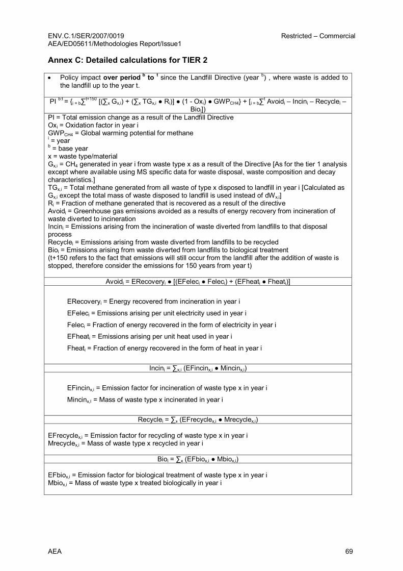
ENV.C.1/SER/2007/0019 Restricted – Commercial AEA/ED05611/Methodologies Report/Issue1
AEA 69
Annex C: Detailed calculations for TIER 2
• Policy impact over period b to t since the Landfill Directive (year b ) , where waste is added to the landfill up to the year t.
PI b:t = i = b∑ t+150 [(∑x Gx,i) + (∑x TGx,i Ri)] (1 Oxi) GWPCH4 + [i = b∑ t Avoidi – Incini – Recyclei – Bioi])
PI = Total emission change as a result of the Landfill Directive Oxi = Oxidation factor in year i GWPCH4 = Global warming potential for methane i = year b = base year x = waste type/material Gx,i = CH4 generated in year i from waste type x as a result of the Directive [As for the tier 1 analysis except where available using MS specific data for waste disposal, waste composition and decay characteristics.] TGx,i = Total methane generated from all waste of type x disposed to landfill in year i [Calculated as Gx,i except the total mass of waste disposed to landfill is used instead of dWx,i] Ri = Fraction of methane generated that is recovered as a result of the directive Avoidi = Greenhouse gas emissions avoided as a results of energy recovery from incineration of waste diverted to incineration Incini = Emissions arising from the incineration of waste diverted from landfills to that disposal process Recyclei = Emissions arising from waste diverted from landfills to be recycled Bioi = Emissions arising from waste diverted from landfills to biological treatment (t+150 refers to the fact that emissions will still occur from the landfill after the addition of waste is stopped, therefore consider the emissions for 150 years from year t)
Avoidi = ERecoveryi [(EFeleci Feleci) + (EFheati Fheati)]
ERecoveryi = Energy recovered from incineration in year i
EFeleci = Emissions arising per unit electricity used in year i
Feleci = Fraction of energy recovered in the form of electricity in year i
EFheati = Emissions arising per unit heat used in year i
Fheati = Fraction of energy recovered in the form of heat in year i
Incini = ∑x,i (EFincinx,i Mincinx,i)
EFincinx,i = Emission factor for incineration of waste type x in year i
Mincinx,I = Mass of waste type x incinerated in year i
Recyclei = ∑x (EFrecyclex,i Mrecyclex,i)
EFrecyclex,i = Emission factor for recycling of waste type x in year i Mrecyclex,i = Mass of waste type x recycled in year i
Bioi = ∑x (EFbiox,i Mbiox,i)
EFbiox,i = Emission factor for biological treatment of waste type x in year i Mbiox,i = Mass of waste type x treated biologically in year i

ENV.C.1/SER/2007/0019 Restricted – Commercial AEA/ED05611/Methodologies Report/Issue1
70 AEA
4.6 Guidelines for the Expost impact assessment of ECCP Measures on the Member State level: Waste Incineration Directive
1. Official title of the directive • Directive 2000/76/EC of the European Parliament and of the Council of 4 December 2000 on
the incineration of waste 2. Short outline of contents and outline of the directive • This Directive aims to regulate the incineration of hazardous waste in order to prevent
excessive pollution to air, water and soil. Incineration and coincineration plants must be authorised, implement measurement and monitoring systems and maximise energy recovery.
• The Waste Incineration Directive has applied to existing plants since December 2005 and to new plants since December 2002. This Directive replaces Directives (89/369/EEC) and (89/429/EEC) on municipal waste incineration and (94/67/EC) on the incineration of hazardous waste. This presents difficulties when establishing a counterfactual against which to evaluate savings, when similar PAMs would have been in place without the Directive under evaluation.
Relevant reporting requirements under the Directive
Commission Decision 2006/329/EC of 20th February 2006 detailed a questionnaire that is to be used for MS to report their implementation of the Directive. The first round of reporting under this decision was due in September 2009.
Combustion plants with a nominal throughput of more than 2 tonnes per hour are required to submit annual reports to their MS competent authority on the functioning and monitoring of the plant. These reports are publicly available. 3. Policy Interaction
EU Policies
• Framework Directive on Waste (75/442/EEC) requires national competent authorities to draw up a waste management plan. One element of the plan encourages recovery of waste including for its use as a source of energy;
• Directives on air pollution from MSW incineration plants (89/369/EEC & 89/429/EEC) regulate the permitting, design, equipment, operation and reporting of waste incineration plant;
• The Combined Heat and Power (CHP) Directive (not yet implemented) aims to indirectly support the advancement of CHP which is commonly used to capture the energy generated through the incineration of MSW.
IMPLICATIONS: The Framework Directive on Waste and the Directives on incineration plants, have focussed attention on waste incineration. However, both these sets of measures were implemented prior to WID. Since the main impact of WID is to enhance energy recovery from incineration and much of the energy recovery is through CHP, the CHP Directive could have a substantial influence on attribution of policy impacts to WID.

ENV.C.1/SER/2007/0019 Restricted – Commercial AEA/ED05611/Methodologies Report/Issue1
AEA 71
National Policies
According to the ECCP Database on Policies and Measures in Europe, there are four MS with national policies related to incineration: Austria, Belgium, Denmark and Spain:
Spain National Integrated Plan for Residual Waste 2008 2012 (PNIR)
France Waste plan Italy Bio digradable waste Malta Mechanical biological treatment plants for solid
waste Poland recovery and recycling of waste Poland implementation of biological wastewater treatment
processes Poland reduction of energy intensity in wastewater
treatment processes Slovenia Decree on landfill of waste, Decree on
environmental tax for environmental pollution caused by waste disposal
Slovakia Measures in waste disposal Source: ECCP Database on Policies and Measures in Europe , http://www.oeko.de/service/pam/
4. IPCC emission categories affected • IPCC category: 1A1a Waste to energy plants, 6.C for waste oil • CO2, CH4
5. Methodological approach
TIER 1
The Tier 1 assessment of the policy impact of the Waste Incineration Directive over the period since its implementation is estimated by taking the following steps:
• Calculating the relative energy recovery rate per unit mass of MSW incinerated using the mass of waste incinerated and the energy from MSW incineration available for final consumption.
• Establishing the energy recovered from waste in the absence of WID by assuming that the recovery rate would have remained at 2005 values.
• Apportion that energy to electricity or heat based on the energy recovered as electricity and heat by the Confederation of European Waste to Energy Plants.
• The emission factor of electricity is calculated for the tier 1 methodology as the EU27 emission factor. The counterfactual emission factor for heat is taken as a gas fired boiler with an efficiency of 85%.
• The energy from waste is then considered to offset energy at the average emission factors calculated.
Appendix A provides a detailed description of the methodologies described above and details of the calculations performed can be found in appendix B.
TIER 2
The Tier 2 methodology attempts to refine the Tier 1 methodology.
• Autonomous developments in the recovery of energy from incineration are taken into account. The linear trend in energy recovery is calculated for the period 1995 to 2004 and extrapolated forward to provide a counterfactual.
• MS specific emission factors for electricity and heat are calculated.

ENV.C.1/SER/2007/0019 Restricted – Commercial AEA/ED05611/Methodologies Report/Issue1
72 AEA
Appendix A provides a detailed description of the methodologies described above and details of the calculations performed can be found in appendix C.
TIER 3
The next tier of analysis might aim to further determine the impacts of autonomous changes and factors that introduce country specificity. The autonomous changes in energy recovery are likely to be influenced by economics; as energy prices have risen it has become more worthwhile to recover as much energy as possible from the incineration process. Therefore it could be useful to correlate energy recovery with energy prices prior to the Waste Incineration Directive and then use the price of energy to set a baseline for what recovery efficiency may have been achieved had WID not been implemented.
6. Issues to consider for future evaluations § Resolving the most appropriate start date for policy effect. § Consider in more detail the impact of air pollutant abatement technologies on emissions of
greenhouse gases, particularly NOx abatement and its impacts on emissions of N2O.
Annex A: Explanations for main methodological assumptions
TIER 1
Determination of the policy impact since the Waste Incineration Directive
The central premise of this analysis is that the Waste Incineration Directive does not influence the amount of waste disposed of through incineration. However, it does influence the amount of energy recovered from that waste. At the Tier 1 level the relative energy recovery rate per unit mass of waste sent for incineration is calculated use to calculate the GHG emissions avoided through the displacement of electricity and heat. The following assumptions are applied: • As stated previously, the assumption is made that the Waste Incineration Directive does not
influence the amount of waste sent for incineration. • It is assumed that in the absence of the Waste Incineration Directive energy recovery rates per
unit mass incinerated would have remained at 2005 values. • For this tier of analysis, it is assumed that the energy recovered from waste displaces energy in
the form of electricity and heat. The fractions of energy recovered as heat and electricity are assumed to be equal to those for the EU 27.
• Tier 1 approach assumes that waste incineration electricity production is replacing the average European fuel mix (fossils plus nuclear) of the EU27 of public and auto producers. Heat generated from waste incineration is assumed to replace heat generated using a gas fired boiler with an efficiency of 85%.
Uncertainty analysis:
The main uncertainty in the Tier 1 approach arises from the assumption that the rate of energy recovery would remain at 2005 levels in the absence of the policy.
Data sources:
• Eurostat: Municipal Solid Waste disposed through incineration per capita; Population; Solid fuel input to thermal power stations; Oil input to thermal power stations; Gas input to thermal power stations.
• CEWEP, heat and electricity generated from MSW incineration from country profiles. • IPCC, 2006, Emission factors for coal, oil and gas combustion.
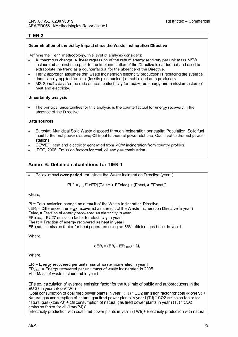
ENV.C.1/SER/2007/0019 Restricted – Commercial AEA/ED05611/Methodologies Report/Issue1
AEA 73
TIER 2
Determination of the policy Impact since the Waste Incineration Directive
Refining the Tier 1 methodology, this level of analysis considers: • Autonomous change. A linear regression of the rate of energy recovery per unit mass MSW
incinerated against time prior to the implementation of the Directive is carried out and used to extrapolate the trend as a counterfactual for the absence of the Directive.
• Tier 2 approach assumes that waste incineration electricity production is replacing the average domestically applied fuel mix (fossils plus nuclear) of public and auto producers.
• MS Specific data for the ratio of heat to electricity for recovered energy and emission factors of heat and electricity.
Uncertainty analysis
• The principal uncertainties for this analysis is the counterfactual for energy recovery in the absence of the Directive.
Data sources
• Eurostat: Municipal Solid Waste disposed through incineration per capita; Population; Solid fuel input to thermal power stations; Oil input to thermal power stations; Gas input to thermal power stations.
• CEWEP, heat and electricity generated from MSW incineration from country profiles. • IPCC, 2006, Emission factors for coal, oil and gas combustion.
Annex B: Detailed calculations for TIER 1
• Policy impact over period b to t since the Waste Incineration Directive (year b )
PI b:t = i = b∑ t dERi[(Feleci EFeleci) + (Fheati EFheati)]
where,
PI = Total emission change as a result of the Waste Incineration Directive dERi = Difference in energy recovered as a result of the Waste Incineration Directive in year i Feleci = Fraction of energy recovered as electricity in year i EFeleci = EU27 emission factor for electricity in year i Fheati = Fraction of energy recovered as heat in year i EFheati = emission factor for heat generated using an 85% efficient gas boiler in year i
Where,
dERi = (ERi – ER2005) * Mi
Where,
ERi = Energy recovered per unit mass of waste incinerated in year I ER2005 = Energy recovered per unit mass of waste incinerated in 2005 Mi = Mass of waste incinerated in year i
EFeleci, calculation of average emission factor for the fuel mix of public and autoproducers in the EU 27 in year t (kton/TWh) = (Coal consumption of coal fired power plants in year i (TJ) * CO2 emission factor for coal (kton/PJ) + Natural gas consumption of natural gas fired power plants in year i (TJ) * CO2 emission factor for natural gas (kton/PJ) + Oil consumption of natural gas fired power plants in year i (TJ) * CO2 emission factor for oil (kton/PJ))/ (Electricity production with coal fired power plants in year i (TWh)+ Electricity production with natural
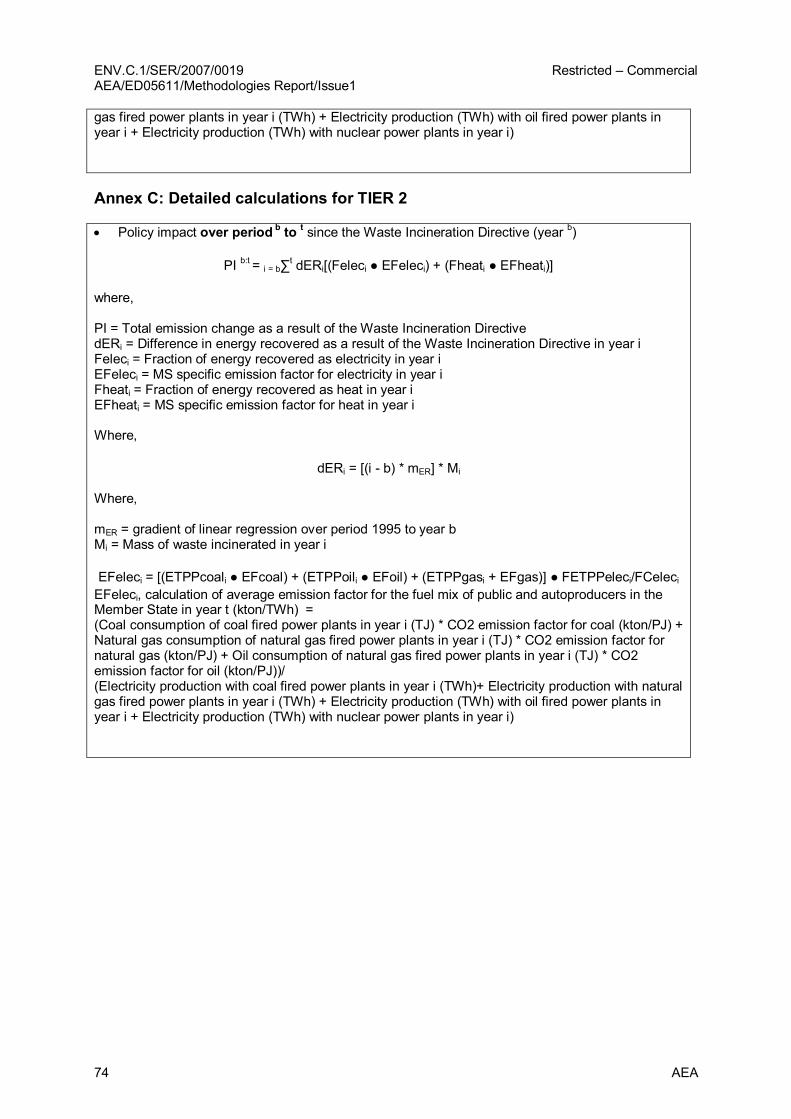
ENV.C.1/SER/2007/0019 Restricted – Commercial AEA/ED05611/Methodologies Report/Issue1
74 AEA
gas fired power plants in year i (TWh) + Electricity production (TWh) with oil fired power plants in year i + Electricity production (TWh) with nuclear power plants in year i)
Annex C: Detailed calculations for TIER 2
• Policy impact over period b to t since the Waste Incineration Directive (year b )
PI b:t = i = b∑ t dERi[(Feleci EFeleci) + (Fheati EFheati)]
where,
PI = Total emission change as a result of the Waste Incineration Directive dERi = Difference in energy recovered as a result of the Waste Incineration Directive in year i Feleci = Fraction of energy recovered as electricity in year i EFeleci = MS specific emission factor for electricity in year i Fheati = Fraction of energy recovered as heat in year i EFheati = MS specific emission factor for heat in year i
Where,
dERi = [(i b) * mER] * Mi
Where,
mER = gradient of linear regression over period 1995 to year b Mi = Mass of waste incinerated in year i
EFeleci = [(ETPPcoali EFcoal) + (ETPPoili EFoil) + (ETPPgasi + EFgas)] FETPPeleci/FCeleci EFeleci, calculation of average emission factor for the fuel mix of public and autoproducers in the Member State in year t (kton/TWh) = (Coal consumption of coal fired power plants in year i (TJ) * CO2 emission factor for coal (kton/PJ) + Natural gas consumption of natural gas fired power plants in year i (TJ) * CO2 emission factor for natural gas (kton/PJ) + Oil consumption of natural gas fired power plants in year i (TJ) * CO2 emission factor for oil (kton/PJ))/ (Electricity production with coal fired power plants in year i (TWh)+ Electricity production with natural gas fired power plants in year i (TWh) + Electricity production (TWh) with oil fired power plants in year i + Electricity production (TWh) with nuclear power plants in year i)

ENV.C.1/SER/2007/0019 Restricted – Commercial AEA/ED05611/Methodologies Report/Issue1
AEA 75
4.7 Guidelines for the Expost impact assessment of ECCP Measures on the Member State level: reform of the sheep and goat meat regime and beef sector premia under CAP
1. Official title of the directive • CAP reform is considered to be mostly encapsulated within: Council Regulation (EC) No 1782/2003 of
29 September 2003 establishing common rules for direct support schemes under the common agricultural policy and establishing certain support schemes for farmers.
• The CAP itself comprises a number of elements directly governing agricultural production in the EU, which are aspects of Regulation 1782/2003 rather than separate legislation. These include the beef and cow premiums, milk quota, set aside and sheep quotas and premiums although a number of other policies and measures remain part of the CAP at the current time.
2. Short outline of contents and outline of the directive • The central aim of the 2003 CAP reform was to ensure, through the ‘decoupling’ of support payments,
that farmers need no longer manage their businesses with the aim of maximising their subsidies from the CAP, but can gear their production and management practices to market demand. The vast majority of support payments under the reformed CAP are independent of production.
• The reformed CAP comprises a single farm payment for EU farmers, which is linked to environmental, food safety, animal and plant health and animal welfare standards, and the requirement to keep all farmland in good agricultural and environmental condition (GAEC).
• Where farmers fail to meet those standards, i.e. non compliance, the direct payments they can claim are reduced or even withdrawn completely for the year concerned. This ‘crosscompliance’ links direct payments to farmers to their respect of environmental and other requirements set at EU and national levels.
• The 2003 reform has the potential to impact upon emissions of greenhouse gases in a number of ways. This includes: a change in livestock numbers (e.g. reduced intensity because payments are no longer linked to production), change in inputs including fertilisers (e.g. maximising profit & efficiency of inputs rather than volume of outputs, especially in the light of increasing costs), improved environmental practices (because of crosscompliance: statutory management requirements (SMRs) and GAEC), and maintenance of grassland and seminatural area (because of setaside and obligation on MSs to retain certain permanent pasture). Reductions in emissions of CH4 and N2O will result from reductions in livestock numbers, improved manure management and reduction in fertiliser use. CO2 reductions will arise from reductions in energy intensity of agriculture, promotion of biomass crops (permitted through 1782/2003 and 795/2004) and increased CO2 sequestration in vegetation and soils by retention of grassland/seminatural areas, and more organic matter in soils.
• To make the evaluation of the 2003 CAP reform more manageable it is useful to consider the individual elements of the CAP and their status before and after the 2003 reform (Council Regulation 1782/2003), rather than all elements of the reform together. Consequently two elements of the coupled Common Agricultural Policy are considered within these guidelines: the sheep and goat meat regime and the beef sector premia. Whilst some of the issues considered within these guidelines are relevant to other elements of the CAP, it is likely that additional issues, not considered within these guidelines, are also important. For example, the impacts of the CAP on carbon sequestration are not considered here.
Relevant reporting requirements under the Directive
• The Farm Accountancy Data Network (FADN) was founded in 1965 to record financial statistics pertaining the farms in the EU and help analyse the economic impact of the CAP. The FADN records detailed economic information for a sample of agricultural holdings representing around 90% of the total agricultural production of the EU. It does not record any environmental information, but the statistical data on agricultural holdings is potential useful for examining changes in emissions causing activities.

ENV.C.1/SER/2007/0019 Restricted – Commercial AEA/ED05611/Methodologies Report/Issue1
76 AEA
Timeline
450
470
490
510
530
550
570
590
610
1980 1985 1990 1995 2000 2005
Total G
HG emission
s from
agr
iculture
(Mt C
O 2 eq)
86
88
90
92
94
96
98
100
102
104
106
Total a
gricultural p
rodu
ction inde
x (100
= 199
9 2
001 av
erag
e)
Agri. emissions Prodn. index
1992 Reform
1999 Reform
2003 Reform
1.
1. IPPC Directive [1996/61/EC]
Into effect
450
470
490
510
530
550
570
590
610
1980 1985 1990 1995 2000 2005
Total G
HG emission
s from
agr
iculture
(Mt C
O 2 eq)
86
88
90
92
94
96
98
100
102
104
106
Total a
gricultural p
rodu
ction inde
x (100
= 199
9 2
001 av
erag
e)
Agri. emissions Prodn. index
1992 Reform
1999 Reform
2003 Reform
1. 1.
1. IPPC Directive [1996/61/EC] 1. IPPC Directive [1996/61/EC]
Into effect
3. Policy Interaction
EU Policies
• As is illustrated by the policy timeline, the 2003 reform of CAP was preceded by reforms in 1992 and 1999. Nonetheless, it is important to recognise that the CAP has been in place for a number of years.
• Compulsory cross compliance was another major element of the CAP reform in 2003 This was the process whereby payment of the single farm payment is dependant on maintaining all land in good agricultural and environmental condition (GAEC) and, where relevant, complying with (largely existing) legislation affecting agricultural management. In this way the 2003 CAP reform Council Regulation 1782/2003 created a direct link with existing environmental, food safety and animal and plant health legislation. Of particular significance is the Nitrates Directive 91/676/EEC, whose main goal is to prevent water pollution caused by N2O stemming from agricultural waste and the excessive use of fertilisers.
IMPLICATIONS: For the purposes of this analysis some of the changes in fertiliser consumption within the EU can be attributed to the Nitrates Directive, therefore analysis of the 2003 CAP reform must interact closely with the analysis of the Nitrates Directive to minimise overlap.
National Policies
• At the National level, only 4 MS from the EU 15 reported relevant PAMs that were in existence prior to CAP reform, these were: Austria, France, Germany and Spain. 23
IMPLICATIONS: The interaction between national policies and EU CAP reform should be treated by the Tier 3 analysis. 4. IPCC emission categories affected • IPCC category: 4 Agricultural emissions (specifically, 4A Enteric fermentation, 4B Manure
management, 4D Emission from soils) 5B (Cropland – sequestration in soils and vegetation), 5C (Grassland – sequestration in soils and vegetation) and 1.A.4.C Emissions from energy use in
23 EEA, Greenhouse gas emission trends and projections in Europe 2007; Tracking progress towards Kyoto targets.
ENV.C.1/SER/2007/0019 Restricted – Commercial AEA/ED05611/Methodologies Report/Issue1
AEA 77
agriculture/forestry/fisheries. Overlap with the Nitrates Directive is mostly reflected in category 4D. • For the reforms to the sheep and beef sector the most important impact categories are 4A and 4B • CH4, CO2 and N2O 5. Methodological approach
TIER 1
The methodology proposed for a Tier 1 assessment of the 2003 CAP reform relies on the assumption that all changes in the number of animals (sheep and cattle), and the associated change in GHG emissions, can be attributed directly to the decoupling of the sheep and beef premia. This assumes that the number of animals would remain at the prereform levels in the absence of the policy. The data used for this assessment is: Total emissions of greenhouse gases from enteric fermentation and manure management from sheep and nondairy cattle, respectively, and, total animal numbers.
The Tier 1 assessment of the policy impact of the 2003 CAP reform in the sheep and beef sector, over the period since its implementation, is calculated using the following calculation:
• Tier 1 counterfactual scenario: The number of animals and the associated emissions per animal is assumed to remain ‘frozen’ at 2004 levels in the absence of the CAP reform.
The Tier 1 approach assumes that the Directive implemented consistently within all Member States, and that the Directive is the main driver of animal numbers within the sector. No adjustments are made for changes in the structure of the livestock enterprises in the Tier 1 approach. Likewise, no corrections are made for the influence of climatic factors or other exogenous variables e.g. animal disease. Importantly, the Tier 1 approach takes no account of autonomous development, or the influence or exogenous variable such as market prices on production. Emissions are based upon Member States submissions to UNFCCC, with no adjustment made for differences in the methodologies applied.
Some important methodological issues remain unresolved in the Tier 1 approach. Consequently, we suggest that the Tier 1 approach should not be considered an accurate representation of the greenhouse gas impacts that can be attributed to the 2003 CAP reform, without further corrections.
Appendix A provides a detailed description of the methodology described above and proposed calculations are listed in Appendix B.
TIER 2
The Tier 2 calculation adjusts for delays in the date of implementation of the requirements of the Directive within Member States.
In addition, as a sensitivity analysis the impact of autonomous development in sector are analysed.
• Tier 2 counterfactual scenario: The linear trend in animal numbers for the period prior to the 2003 reform is assumed to continue to the present i.e. account is taken for any underlying trends in production that will not be captured within a ‘frozen efficiency’ counterfactual.
Some important methodological issues remain unresolved in the Tier 2 approach. Importantly no adjustments are made for the impact of market conditions on production (although this may be reflected to some extent in the assessment of autonomous development). Since the CAP reform, by its very design, aims to make production more responsive to market demand, then this is a major limitation with the Tier 2 approach. In addition, the Tier 2 approach does not correct for structural changes such as the make up of animal populations (which may or may not be influenced by the Reforms), or policy overlaps.
On this basis we consider that the results from the Tier 2 approach should be treated with caution. The results do provide an indication of the possible magnitude of the policy savings from the reforms, and from reductions in GHG emissions from the livestock sector more generally, but uncorrected the results are likely to misrepresent the true impacts of the policy. Most importantly, how the CAP reform interacts with the

ENV.C.1/SER/2007/0019 Restricted – Commercial AEA/ED05611/Methodologies Report/Issue1
78 AEA
market for agricultural commodities, and in turn how this influence production, is not explicitly considered. Therefore, we do not consider the results sufficiently robust to recommend the use of a Tier 1 or Tier 2 approach to quantify the impacts of the CAP Reform.
Appendix A provides a detailed description of the methodologies described above and proposed calculations are listed in Appendix C.
TIER 3
A tier 3 analysis would aim to determine the impacts of CAP reform using detailed data sets on agricultural processes, such as:
• Statistics on the changes in the structure of livestock enterprises both prior to and following the CAP reform. Using the IPCC emissions factors and methodologies, it may be possible to isolate the impact of these structural changes on overall emissions from the sector.
• The impact of market conditions (e.g. price of farm inputs, and farm commodities) needs to be considered. As far as possible the relationship between the key market parameters and production should be analysed. This is likely to require the development of existing or new econometric models.
• The full range of emissions arising from livestock enterprises need to be considered within the Tier 3 approach. In particular, emissions arising from application of animal manures to land, and energy use at farming enterprises needs to be consider. This will require some ‘allocation’ of the overall emissions to the various farm enterprises or commodities.
• The interaction of CAP reform with other national and EU policies may be difficult to quantify. It may therefore be more appropriate to consider the policies, and associated impacts, as part of a package.
6. Issues to consider for future evaluations The availability of data is crucial to evaluation of the GHG impacts of policy. Currently, the Commission is reviewing the reporting that takes place under the CAP to include an assessment of the GHG impact within each MS. Clearly, such as development would be highly valuable for future evaluations.
A further issue relates to the uncertainty in the emission factors and emission inventories for the agricultural sector. The use of default emissions factors, and the large uncertainty in these factors, means that Member States emission inventories may not adequately capture the impacts of certain abatement measures (e.g. manure management, feed management) on overall emissions.
ENV.C.1/SER/2007/0019 Restricted – Commercial AEA/ED05611/Methodologies Report/Issue1
AEA 79
Annex A: Explanations for main methodological assumptions
TIER 1
Determination of the policy impact in the sheep and beef sector since CAP reform
The underlying assumption of this analysis is that CAP reform has altered the number of animals and the associated GHG emissions. Therefore, the statistics considered here are the emissions from enteric fermentation and manure management at sheep and nondairy cattle enterprises. The counterfactual for this Tier 1 analysis makes the assumption that the number of animals, and the emissions per head, would have remained at 2004 levels in the absence of the 2003 CAP reform.
Uncertainty analysis
The first uncertainty in the Tier 1 approach arises from the counterfactual scenario for livestock numbers in the absence of the CAP reform. ‘Freezing’ the animal numbers, and emissions per head, in this way is likely to be a significant simplification. The Tier 2 analysis should aim to implement a more complex counterfactual. A second uncertainty lies in the extent to which structural effects e.g. the number of ewes or suckler cows, has influenced overall emissions from the sector.
Since only emissions from enteric fermentation and manure management are used to calculate the emissions, this may lead to an underestimate of the overall impacts. In particular, emissions associated with the application of animal manures to soil are not captured. A further uncertainty relates to the methodologies used by Member States to calculate emissions from the sector, where no adjustment is made for the different methodologies.
Policy overlaps are not explicitly considered in the Tier 1 approach.
Data sources:
UNFCCC: Greenhouse gas emissions from agriculture Greenhouse gas emissions data is (currently) available up to the year 2006.
ENV.C.1/SER/2007/0019 Restricted – Commercial AEA/ED05611/Methodologies Report/Issue1
80 AEA
TIER 2
Determination of the policy impact since CAP reform
As for the Tier 1 analysis, the underlying assumption is that CAP reform has altered the number of animals and the associated GHG emissions. Accordingly, the statistics considered here are also the emissions from enteric fermentation and manure management from sheep and nondairy cattle. In the Tier 2 analysis an adjustment is made to the policy start date to reflect the fact that not all Member States implemented to requirements of the Directive at the same time.
Sensitivity analysis An alternative counterfactual can be calculated by extrapolating the linear trend in the animal numbers from the 3 years prior to the implementation of the regulations. Accordingly, it is assumed that the trend in animal numbers is linear and that the trend would have continued unchanged if CAP reform had not been implemented. This provides a crude assessment of any autonomous progress (which may include the influence of consumer trends, and market conditions).
Uncertainties
Various economic drivers (such as consumer demand) may have significantly influenced production with the sector. These factors are not accounted for in this Tier 2 analysis, however, it is important these factors are included in the counterfactual for the Tier 3 methodology. Also structural changes have not been addressed within the Tier 2 approach, but could potentially be included in the future with more disaggregated data. Likewise, emissions associated with the application of animal manures to soil could be included within a Tier 2 approach with more detailed data on the methodologies and data used within national inventories. Policy overlaps are also not explicitly considered.
Data sources:
UNFCCC: Greenhouse gas emissions from agriculture is (currently) available up to the year 2006.
TIER 3
In a Tier 3 approach, as far a possible all influencing variables upon production should be isolated and corrected for. In particular, the analysis should distinguish two situations:
effects of the policy change (switch from the coupled support to decoupled support) i.e. the relative change in production from moving from coupled to decoupled support under the given market conditions
effects of exogenous factors on the level of production (since market factors such as commodity prices would influence production under both a coupled and decoupled arrangement – although on a differential basis).
One approach would be to use a linear regression model to examine the impact of the key influencing variables over the period prior to CAP reform, using the predictors GDP, population, oil price, cost of animal feed and commodity prices. Then using the reported values for these predictors in the period since the implementation of CAP reform, a more accurate counterfactual could be constructed.
Bottom up data could also be used to refine or calibrate the results, for example, information on feed intake, ages of animals and manure management practices are all potential important. Likewise information on animal disease may also be important to correct for.
Alternatively, existing econometric models for the agricultural sector could be used to determine the impact of the reforms on production, and the influence of the other deterministic variables. If an environmental module is not already included within the model, then the outputs from the model could be analyses offmodel to determine the impacts on GHG emissions.
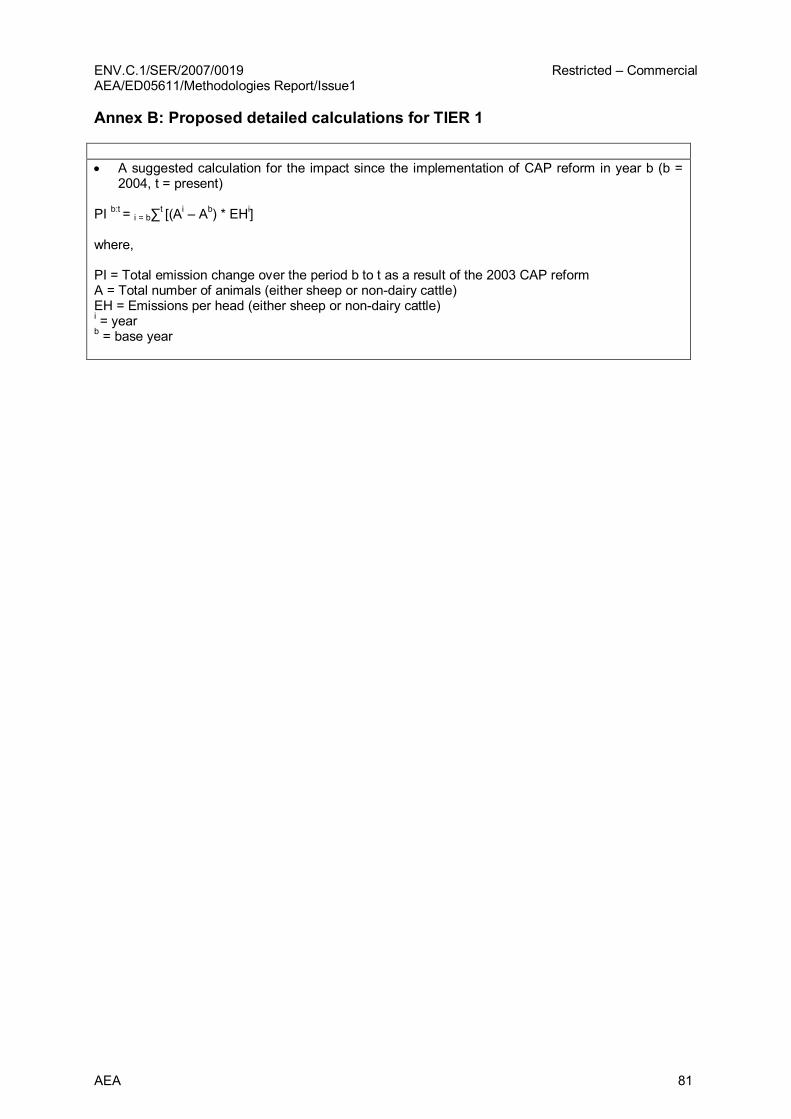
ENV.C.1/SER/2007/0019 Restricted – Commercial AEA/ED05611/Methodologies Report/Issue1
AEA 81
Annex B: Proposed detailed calculations for TIER 1
• A suggested calculation for the impact since the implementation of CAP reform in year b (b = 2004, t = present)
PI b:t = i = b∑ t [(A i – A b ) * EH i ]
where,
PI = Total emission change over the period b to t as a result of the 2003 CAP reform A = Total number of animals (either sheep or nondairy cattle) EH = Emissions per head (either sheep or nondairy cattle) i = year b = base year
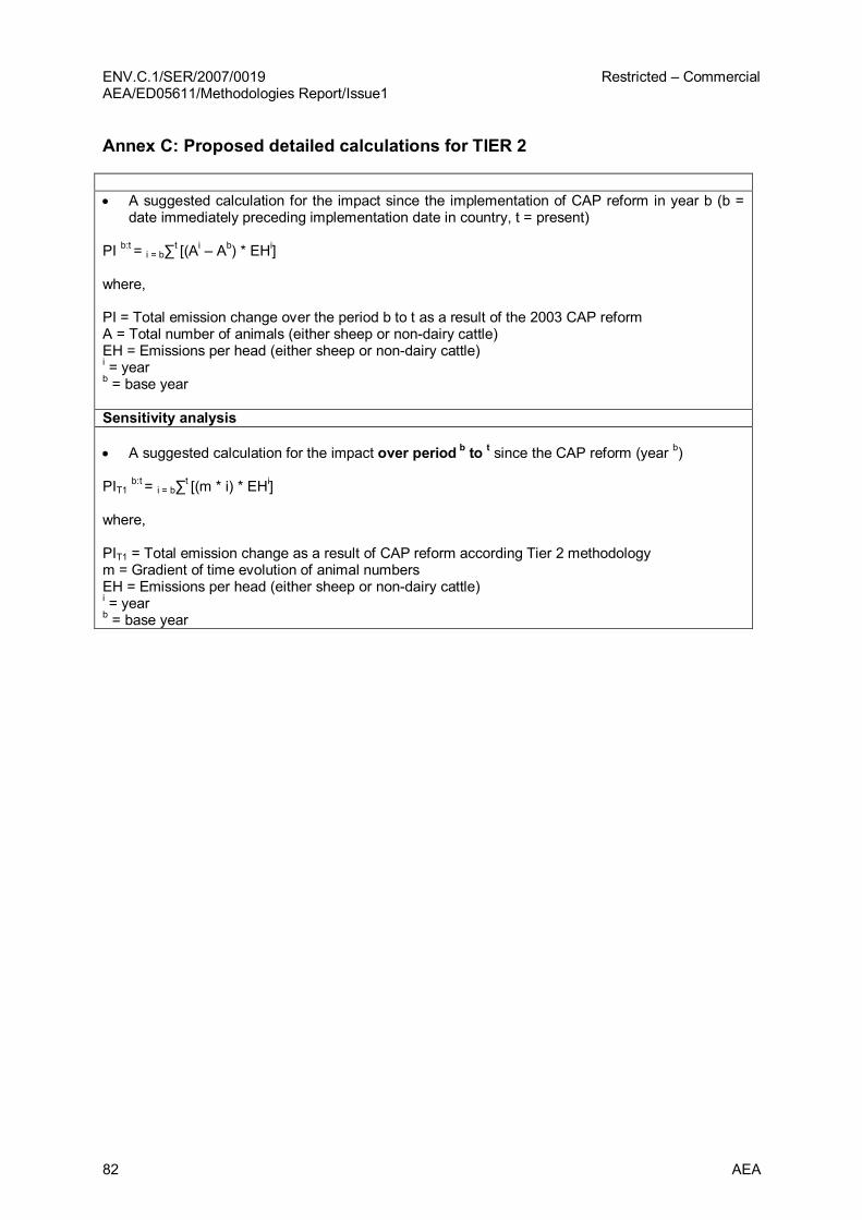
ENV.C.1/SER/2007/0019 Restricted – Commercial AEA/ED05611/Methodologies Report/Issue1
82 AEA
Annex C: Proposed detailed calculations for TIER 2
• A suggested calculation for the impact since the implementation of CAP reform in year b (b = date immediately preceding implementation date in country, t = present)
PI b:t = i = b∑ t [(A i – A b ) * EH i ]
where,
PI = Total emission change over the period b to t as a result of the 2003 CAP reform A = Total number of animals (either sheep or nondairy cattle) EH = Emissions per head (either sheep or nondairy cattle) i = year b = base year
Sensitivity analysis
• A suggested calculation for the impact over period b to t since the CAP reform (year b )
PIT1 b:t = i = b∑ t [(m * i) * EH i ]
where,
PIT1 = Total emission change as a result of CAP reform according Tier 2 methodology m = Gradient of time evolution of animal numbers EH = Emissions per head (either sheep or nondairy cattle) i = year b = base year
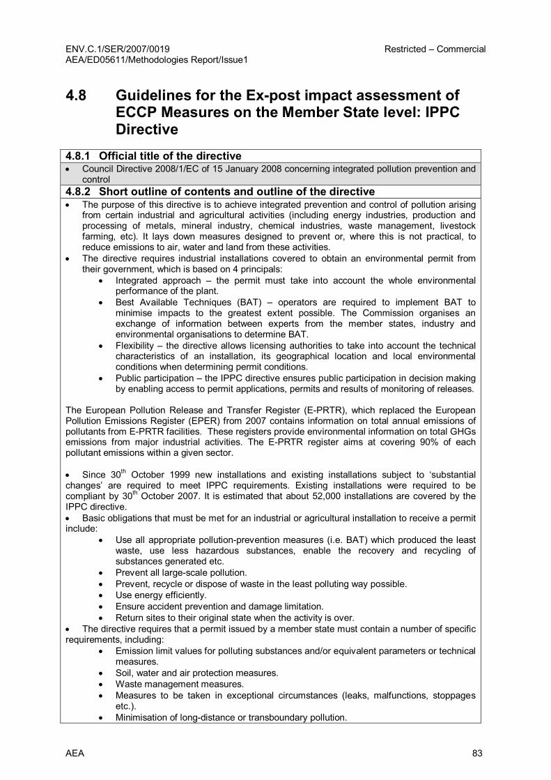
ENV.C.1/SER/2007/0019 Restricted – Commercial AEA/ED05611/Methodologies Report/Issue1
AEA 83
4.8 Guidelines for the Expost impact assessment of ECCP Measures on the Member State level: IPPC Directive
4.8.1 Official title of the directive • Council Directive 2008/1/EC of 15 January 2008 concerning integrated pollution prevention and
control 4.8.2 Short outline of contents and outline of the directive • The purpose of this directive is to achieve integrated prevention and control of pollution arising
from certain industrial and agricultural activities (including energy industries, production and processing of metals, mineral industry, chemical industries, waste management, livestock farming, etc). It lays down measures designed to prevent or, where this is not practical, to reduce emissions to air, water and land from these activities.
• The directive requires industrial installations covered to obtain an environmental permit from their government, which is based on 4 principals:
• Integrated approach – the permit must take into account the whole environmental performance of the plant.
• Best Available Techniques (BAT) – operators are required to implement BAT to minimise impacts to the greatest extent possible. The Commission organises an exchange of information between experts from the member states, industry and environmental organisations to determine BAT.
• Flexibility – the directive allows licensing authorities to take into account the technical characteristics of an installation, its geographical location and local environmental conditions when determining permit conditions.
• Public participation – the IPPC directive ensures public participation in decision making by enabling access to permit applications, permits and results of monitoring of releases.
The European Pollution Release and Transfer Register (EPRTR), which replaced the European Pollution Emissions Register (EPER) from 2007 contains information on total annual emissions of pollutants from EPRTR facilities. These registers provide environmental information on total GHGs emissions from major industrial activities. The EPRTR register aims at covering 90% of each pollutant emissions within a given sector.
• Since 30 th October 1999 new installations and existing installations subject to ‘substantial changes’ are required to meet IPPC requirements. Existing installations were required to be compliant by 30 th October 2007. It is estimated that about 52,000 installations are covered by the IPPC directive. • Basic obligations that must be met for an industrial or agricultural installation to receive a permit include:
• Use all appropriate pollutionprevention measures (i.e. BAT) which produced the least waste, use less hazardous substances, enable the recovery and recycling of substances generated etc.
• Prevent all largescale pollution. • Prevent, recycle or dispose of waste in the least polluting way possible. • Use energy efficiently. • Ensure accident prevention and damage limitation. • Return sites to their original state when the activity is over.
• The directive requires that a permit issued by a member state must contain a number of specific requirements, including:
• Emission limit values for polluting substances and/or equivalent parameters or technical measures.
• Soil, water and air protection measures. • Waste management measures. • Measures to be taken in exceptional circumstances (leaks, malfunctions, stoppages
etc.). • Minimisation of longdistance or transboundary pollution.

ENV.C.1/SER/2007/0019 Restricted – Commercial AEA/ED05611/Methodologies Report/Issue1
84 AEA
• Release Monitoring. • A permit issued in compliance of the IPPC directive shall not contain emission limit values for greenhouse gases if they are subject to the EU Emissions Trading Scheme.
Relevant reporting requirements under the Directive
• Member States are required by this directive to send the Commission every three years the available representative data on the limit values applied to specific category of activities covered by the directive and, where appropriate, the BAT from which these values are derived.
• The Commission is required to organise an exchange of information between Member States and industry concerning BAT, associated monitoring and development in them. The Commission is required to report on this process every three years. In practice, this requirement has taken the form of the BAT Reference Document determination process.
• Reports on the implementation of the Directive and its effectiveness are required. The first and second report has now been published.
• At the end of 2005 the Commission launched in its first IPPC report a review process of the IPPC Directive and related legislation on industrial emissions. As a result of the review on 21 December 2007 the Commission adopted a Proposal for a Directive on industrial emissions. The Proposal recasts seven existing Directives related to industrial emissions, including the IPPC Directive, into a single clear and coherent legislative instrument.
4.8.3 Policy Interaction
EU Policies
• Since 1999 the VOC solvents Directive (SED) has interacted closely with the IPPC Directive. The SED requires installations in which such activities are applied to comply either with emission limit values set out in the Directive or with the requirements of the socalled reduction scheme. The Directive sets out emission limit values for VOCs in waste gases and maximum levels for fugitive emissions (expressed as percentage of solvent input) or total emission limit values.
• Since 2000, the waste incineration Directive (WID) has interacted closely with the IPPC Directive. The aim of the WID is to prevent or to reduce as far as possible negative effects on the environment caused by the incineration and coincineration of waste. In particular, it should reduce pollution caused by emissions into the air, soil, surface water and groundwater, and thus lessen the risks which these pose to human health. The WI Directive sets emission limit values and monitoring requirements for pollutants to air such as dust, nitrogen oxides (NOx), sulphur dioxide (SO2), hydrogen chloride (HCl), hydrogen fluoride (HF), heavy metals and dioxins and furans.
• At the EU level, since 2001, the Large Combustion Plant Directive (LCPD) has interacted closely with the IPPC Directive. The LCPD establishes emission limits for SO2, NOx and particulate matter from large combustion plants >50MW.
• The EU ETS, which commenced 1 st January 2005, covers process and energy use emissions from large industrial emitters in the glass and ceramics, pulp and paper, aluminium, ferrous metals and pharmaceutical sectors. The EU ETS Directive amended the IPPC Directive such that, when an installation is participating in the EU ETS, IPPC emission limits are not set for any GHGs covered by the EU ETS unless required to prevent local pollution problems. In addition, for activities listed in Annex I of the EU ETS Directive, MS are not required to impose energy efficiency requirements in respect of combustion units or other units emitting carbon dioxide on the site under the IPPC. As a result, an assessment of the policy impact of the IPPC Directive will also be influenced by the EU ETS.
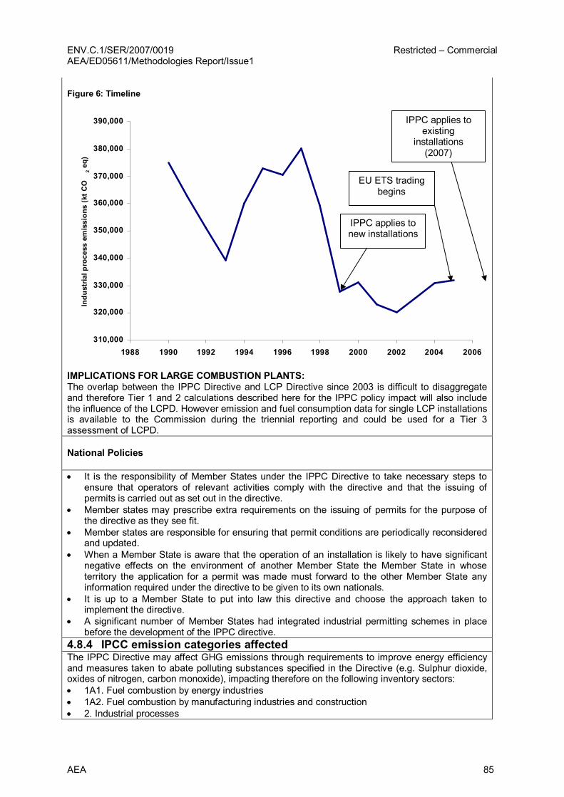
ENV.C.1/SER/2007/0019 Restricted – Commercial AEA/ED05611/Methodologies Report/Issue1
AEA 85
Figure 6: Timeline
310,000
320,000
330,000
340,000
350,000
360,000
370,000
380,000
390,000
1988 1990 1992 1994 1996 1998 2000 2002 2004 2006
Indu
stria
l process emission
s (kt C
O
2 eq
)
IMPLICATIONS FOR LARGE COMBUSTION PLANTS: The overlap between the IPPC Directive and LCP Directive since 2003 is difficult to disaggregate and therefore Tier 1 and 2 calculations described here for the IPPC policy impact will also include the influence of the LCPD. However emission and fuel consumption data for single LCP installations is available to the Commission during the triennial reporting and could be used for a Tier 3 assessment of LCPD.
National Policies
• It is the responsibility of Member States under the IPPC Directive to take necessary steps to ensure that operators of relevant activities comply with the directive and that the issuing of permits is carried out as set out in the directive.
• Member states may prescribe extra requirements on the issuing of permits for the purpose of the directive as they see fit.
• Member states are responsible for ensuring that permit conditions are periodically reconsidered and updated.
• When a Member State is aware that the operation of an installation is likely to have significant negative effects on the environment of another Member State the Member State in whose territory the application for a permit was made must forward to the other Member State any information required under the directive to be given to its own nationals.
• It is up to a Member State to put into law this directive and choose the approach taken to implement the directive.
• A significant number of Member States had integrated industrial permitting schemes in place before the development of the IPPC directive.
4.8.4 IPCC emission categories affected The IPPC Directive may affect GHG emissions through requirements to improve energy efficiency and measures taken to abate polluting substances specified in the Directive (e.g. Sulphur dioxide, oxides of nitrogen, carbon monoxide), impacting therefore on the following inventory sectors: • 1A1. Fuel combustion by energy industries • 1A2. Fuel combustion by manufacturing industries and construction • 2. Industrial processes
IPPC applies to new installations
IPPC applies to existing
installations (2007)
EU ETS trading begins

ENV.C.1/SER/2007/0019 Restricted – Commercial AEA/ED05611/Methodologies Report/Issue1
86 AEA
4.8.5 Methodological approach
TIER 1
Assessment of the policy impact since the implementation of the IPPC Directive assumes that the IPPC Directive covers the majority of installations whose emissions are accounted for in the sectors listed above.
• Step 1: The emission rate per unit industrial production is calculated using the total emissions of greenhouse gases from industrial processes and the industrial production index. EU average industrial production index data is used to calculate emissions intensity where MS specific data is unavailable
• Step 2: The emissions intensity of energy industries and of energy used in Manufacturing Industries and Construction is calculated using the total emissions of GHG from the sectors and corresponding fuel consumption data.
• Step 3: The emission rate of energy production in industry (1A2), industrial processes (2) and energy industries (1A1 energy industries) is assumed to remain at the level as at implementation year 1 (the counterfactual).
• Step 4: The emissions intensity in the year of implementation is compared to the emissions intensity in the year of implementation 1.
• Step 5: The difference in emissions intensity is multiplied by the corresponding activity data in order to determine emissions savings in the given year compared to the year of implementation 1.
• Steps 4 and 5 are repeated for each year up to the latest year for which data is available. Appendix A provides a detailed description of the methodologies described above and details of the calculations performed can be found in appendix B.
4.8.6 Issues to consider for future evaluations The Methodology for calculating the impact of the IPPC Directive could be improved in the following ways: • Use industry and installation specific production and emission data to derive trends for the
industries required to comply with IPPC regulation. • Model the emissions baseline in the absence of the IPPC Directive. Important variables for such
models would likely be: o Production o Oil and gas prices o Raw material prices o Industry investment in new technology o Demand curves
• Consider how the requirements of the Directive (e.g. with respect to energy efficiency) have been implemented within different Member States.
ENV.C.1/SER/2007/0019 Restricted – Commercial AEA/ED05611/Methodologies Report/Issue1
AEA 87
4.8.7 Annex A: Explanations for main methodological assumptions
4.8.8 TIER 1
The Tier 1 analysis assumes that the IPPC Directive covers the majority of process emissions from industry. Therefore, examining the relative change in emissions from the sector will yield an estimate of the impact of the IPPC Directive.
Determination of the policy impact
Combining total industrial process emissions and industrial production index values the emission rate per unit production index can be calculated. The calculation then makes the assumption that the emission rate will remain at levels as at implementation year 1.
Uncertainties
The major uncertainties of the Tier 1 analysis are: assumption that the policy impact of the IPPC Directive can be estimated using the total
industrial process emissions assumption that emissions per production index unit would have remained at the
implementation year 1 rate in the absence of the Directive
Data sources
• UNFCCC Categories 1A1, 1A2, 2 emissions and activity data • Eurostat – Industrial Production Index (Volume index of production)
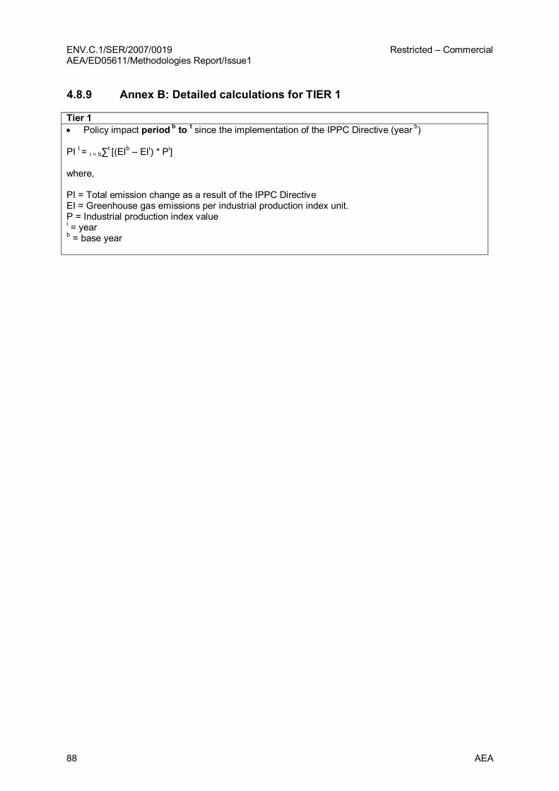
ENV.C.1/SER/2007/0019 Restricted – Commercial AEA/ED05611/Methodologies Report/Issue1
88 AEA
4.8.9 Annex B: Detailed calculations for TIER 1
Tier 1 • Policy impact period b to t since the implementation of the IPPC Directive (year b )
PI t = i = b∑ t [(EI b – EI i ) * P i ]
where,
PI = Total emission change as a result of the IPPC Directive EI = Greenhouse gas emissions per industrial production index unit. P = Industrial production index value i = year b = base year

ENV.C.1/SER/2007/0019 Restricted – Commercial AEA/ED05611/Methodologies Report/Issue1
AEA 89
4.9 Guidelines for the Expost impact assessment of ECCP Measures on the Member State level: Nitrates Directive
1. Official title of the directive • Directive 91/676/EEC of the European Parliament and of the Council of 12 December 1991 concerning
the protection of waters against pollution caused by nitrates from agricultural sources 2. Short outline of contents and outline of the directive • The Nitrates Directive concerns the protection of waters against pollution caused by nitrates from
agricultural sources. The main goal is to prevent nitrogen loading of water bodies stemming from agricultural waste and the excessive use of fertilisers. However, there is a close link between N2O emissions from agricultural soils and nitrate losses resulting in water pollution. Therefore, measures introduced under the Nitrates Directive may also result in declining N2O emissions to the atmosphere.
• The Nitrates Directive requires Member States to identify and designate Nitrate Vulnerable Zones (NVZs) or designate the whole country, to draw up Codes of Good Agricultural Practice (voluntary applied to the whole territory and obligatory in NVZ) and Action Programmes for NVZs. Farmers located in NVZs are required to comply with Action Programme measures to reduce nitrate leaching.
• The designated area of NVZs has expanded with time. In 1999, NVZs represented 35.5% of the total EU 15 area. In 2003 however, the designated area had increased to account for 43.9% for the EU 15 total land area, with many MS increasing their designated area and Ireland declaring its entire territory as an NVZ, joining six other MS that had previously taken this decision. The NVZ designation is currently under review again.
• Reports from the Commission on the implementation of the nitrates directive state a progressive trend towards reduced fertiliser consumption has been recorded since the mideighties 24 .
Relevant reporting requirements under the Directive
• Under the Nitrates Directive, MS are required to submit a report every 4 years to the Commission. • Annex V of the Directive specifies information to be contained in reports to the Commission as required
under Article 10 of the Directive. The report should contain information pertaining to codes of good agricultural practice, designated nitrate vulnerable zones (NVZ), the results of water monitoring and a summary of the relevant aspects of action programmes drawn up in relation to nitrate vulnerable zones. Annex IV of the Directive specifies reference methods for measurement.
24 COM (2007) 120 final, Report from the Commission to the Council and the European Parliament on the implementation of Council Directive 91/676/EEC concerning the protection of waters against pollution caused by nitrates from agricultural sources for the period 2000 – 2003.
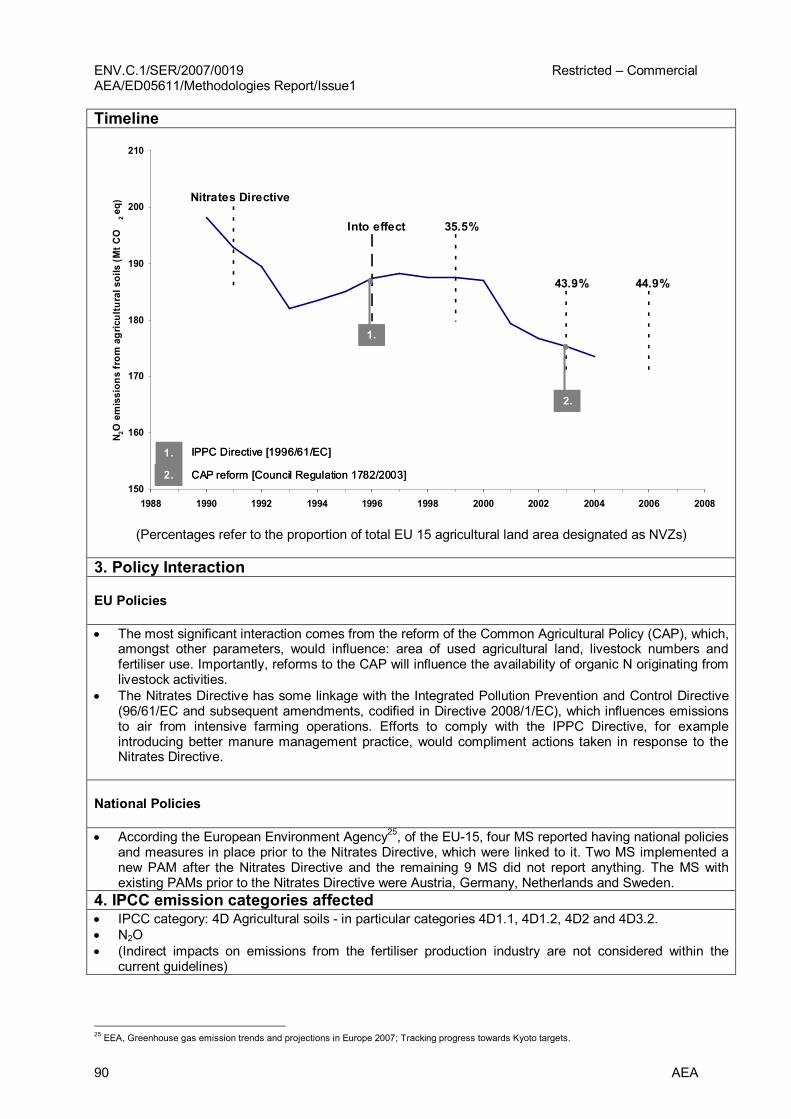
ENV.C.1/SER/2007/0019 Restricted – Commercial AEA/ED05611/Methodologies Report/Issue1
90 AEA
Timeline
150
160
170
180
190
200
210
1988 1990 1992 1994 1996 1998 2000 2002 2004 2006 2008
N 2 O emission
s from
agricultural soils (M
t CO
2 eq
) Nitrates Directive
35.5%
43.9% 44.9%
2.
1.
1.
2.
IPPC Directive [1996/61/EC]
CAP reform [Council Regulation 1782/2003]
Into effect
150
160
170
180
190
200
210
1988 1990 1992 1994 1996 1998 2000 2002 2004 2006 2008
N 2 O emission
s from
agricultural soils (M
t CO
2 eq
) Nitrates Directive
35.5%
43.9% 44.9%
2. 2.
1. 1.
1.
2.
IPPC Directive [1996/61/EC]
CAP reform [Council Regulation 1782/2003]
1.
2.
IPPC Directive [1996/61/EC]
CAP reform [Council Regulation 1782/2003]
Into effect
(Percentages refer to the proportion of total EU 15 agricultural land area designated as NVZs)
3. Policy Interaction
EU Policies
• The most significant interaction comes from the reform of the Common Agricultural Policy (CAP), which, amongst other parameters, would influence: area of used agricultural land, livestock numbers and fertiliser use. Importantly, reforms to the CAP will influence the availability of organic N originating from livestock activities.
• The Nitrates Directive has some linkage with the Integrated Pollution Prevention and Control Directive (96/61/EC and subsequent amendments, codified in Directive 2008/1/EC), which influences emissions to air from intensive farming operations. Efforts to comply with the IPPC Directive, for example introducing better manure management practice, would compliment actions taken in response to the Nitrates Directive.
National Policies
• According the European Environment Agency 25 , of the EU15, four MS reported having national policies and measures in place prior to the Nitrates Directive, which were linked to it. Two MS implemented a new PAM after the Nitrates Directive and the remaining 9 MS did not report anything. The MS with existing PAMs prior to the Nitrates Directive were Austria, Germany, Netherlands and Sweden.
4. IPCC emission categories affected • IPCC category: 4D Agricultural soils in particular categories 4D1.1, 4D1.2, 4D2 and 4D3.2. • N2O • (Indirect impacts on emissions from the fertiliser production industry are not considered within the
current guidelines)
25 EEA, Greenhouse gas emission trends and projections in Europe 2007; Tracking progress towards Kyoto targets.
ENV.C.1/SER/2007/0019 Restricted – Commercial AEA/ED05611/Methodologies Report/Issue1
AEA 91
5. Methodological approach
TIER 1
The tier 1 assessment of the policy impact of the Nitrates Directive over the period since its implementation is calculated using the following calculation:
• Tier 1 counterfactual scenario: The emission rate of N2O from soils per unit area of agricultural land is assumed to remain ‘frozen’ at 1996 levels in the absence of the Nitrates Directive.
The Tier 1 approach assumes that the Directive is implemented consistently within all Member States, and that the Directive is the main driver of Nitrogen application rates within the sector. No adjustments are made for changes in land use, fertiliser, crop or soil types in the Tier 1 approach. Likewise, no corrections are made for the influence of climatic factors on e.g. fertiliser application rates. Furthermore, by assessing impacts on the basis of total agricultural land area no differentiation is made between emissions from soils within NVZs and those outside of NVZs.
Some important methodological issues remain unresolved in the Tier 1 approach. Consequently, we suggest that the Tier 1 approach should not be considered an accurate representation of the greenhouse gas impacts that can be attributed to the Nitrates Directive, without further corrections.
Appendix A provides a detailed description of the methodologies described above and details of the calculations performed can be found in appendix B.
TIER 2
The calculation takes into account the influence of annual weather variations on the N2O emission rate per unit area of land. It also adjusts for delays in the date of implementation of the requirements of the Directive within member states.
• Tier 2 counterfactual scenario: In the absence of the Directive, the N2O emission rate per unit area is assumed to remain ‘frozen’ at the average for the three years prior to the implementation of the Directive within the respective Member State.
Some important methodological issues remain unresolved in the Tier 2 approach. No corrections are made for overlaps with other policy drivers e.g. CAP reform. Structural changes in land use or crop type remain uncorrected, as do corrections for savings outside of NVZs. Furthermore, the influence of price effects (both inputs and outputs) on fertiliser application rates are not isolated from the estimated policy impacts.
As a result of these limitations, we consider that the Tier 2 approach should not be considered an accurate representation of the greenhouse gas impacts that can be attributed to the Nitrates Directive. The results do provide an indication of the overall magnitude of the policy savings from the Directive, and from reductions from N2O emissions from soils more generally, but uncorrected the results are likely to overestimate the true impacts of the policy. Overlaps with the CAP reforms can be addressed by considering the polices together, as a package. However, corrections for structural changes (some of which may be induced by the CAP reform) and the influence of price effects (e.g. fertiliser and commodity prices) will require a more detailed (Tier 3) evaluation methodology.
Appendix A provides a detailed description of the methodologies described above and details of the calculations performed can be found in appendix C.
TIER 3
A Tier 3 approach would aim, as far as possible, to address all of the methodological issues that remain unresolved in the Tier 2 approach. In most cases this will require additional bottom up data collection, and more sophisticated modelling of the main drivers of emissions.
• For example, a Tier 3 analysis might aim to further determine the impacts of details of fertiliser use and N2O emissions within and outside NVZs in each country. A more detailed assessment of the Nitrates
ENV.C.1/SER/2007/0019 Restricted – Commercial AEA/ED05611/Methodologies Report/Issue1
92 AEA
Directive would aim to consider how N2O emissions from soils have varied within designated NVZs. Emission inventories are difficult to obtain at this resolution, however, N2O emissions can be obtained by proxy from fertiliser use data, using an emissions factor of 0.0125 kg N2O/kg fertiliser (N) 26 .
• In order to establish the counterfactual for the nitrates directive with greater accuracy, MS should look to the agricultural standard practices prior to the Nitrates Directive, for example standard practice for cereal crops. This counterfactual could then be compared with the standard practise within NVZs to establish the change in fertiliser usage over a defined area as a result of the Directive. The resultant change in emissions can subsequently be calculated. Within this assessment it is important to take into account different implementation activities in each MS.
• The Nitrates Directive may also have brought about improvements in manure management practices within designated NVZs. Using information on livestock numbers and the manure management technologies in use within NVZs, the impact of this improvement could potentially be quantified.
• The area of designated NVZs varies between MS including seven of the EU 15 that have declared their entire territory, reflecting the different scale of nitrate pollution from agriculture in different MS. It is important this is taken into account when assessing impacts at the MS level.
• Econometric techniques can be used to better understand the relationship between commodity prices and fertiliser prices, on fertiliser application rates. This will require long run data on prices, application rates and production. Previous work 27 found that fertiliser demand was more sensitive to agricultural output demand than its own price.
• Data on changes in land use and crop type within Member States over the period of the Directive can potentially be used to correct for any structural changes that will impact upon the topdown indicator, but are unrelated to the Directive. However, a key challenge will be linking bottomup emissions estimates (i.e. emissions per ha by crop type) with the aggregate data within the inventories.
6. Issues to consider for future evaluations
Uncertainties in the activity data and emissions factors associated with N2O emissions from soils are high. As these methodologies evolve, and the approaches used within Member State inventories improve, the evaluation methodologies will need to evolve accordingly to reflect these changes.
26 EMEP/CORINAIR Emission Inventory Guidebook – 2007, Technical report No 16/2007. (http://reports.eea.europa.eu/EMEPCORINAIR5/en/page002.html) 27
F Bel, G D d’Aubigny, A Lacroix and A Mollard. (2004) Fertiliser taxation and regulation on nonpoint water pollution: a critical analysis based on European experiences. Int. J. Water, vol 2, no 4, 2004, pp 247266
ENV.C.1/SER/2007/0019 Restricted – Commercial AEA/ED05611/Methodologies Report/Issue1
AEA 93
Annex A: Explanations for main methodological assumptions
TIER 1
Determination of the policy impact since the Nitrates Directive came into force
The principal assumption of this analysis is that the Nitrates Directive has not influenced the total area of agricultural land, but through the action measures implemented in NVZs, it has caused a reduction in the N2O emissions arising per unit area of agricultural land. In this Tier 1 analysis a counterfactual history is established for N2O emissions per area of agricultural land in the absence of the Directive. The emissions rate is assumed to remain at 1996 levels, since the Directive was not implemented until 5 years after its agreement.
Uncertainty analysis
The principle uncertainty in the Tier 1 approach arises from the counterfactual for evolution of N2O emissions per area of land in the absence of the Nitrates Directive. The Tier 1 analysis does not take into account the influence of other policies or other exogenous factors on the indicator. It also assumes that for all Member States the start date of the policy is 1996.
Data sources:
Faostat: Total area of agricultural land. UNFCCC: Greenhouse gas emissions from agricultural soils. TIER 2
Determination of the policy impact since the Nitrates Directive
Tier 2 corrects for the fact that not all Member States will have implemented the Directive at the same time. In addition, a further correction is made to reflect that fact that climatic factors (e.g. weather) can influence the fertiliser application rates, and therefore N2O emission rates. Making the following assumptions allows refinement of the impact of the Nitrates Directive on GHG emissions from agricultural soils:
• The start date of the policy within a given Member State is assumed to begin from the date that the first Action Programme is implemented.
• To correct for climatic factors the preDirective rate of emissions per unit area of agricultural land is assumed to be’ frozen’ at an average of the rate in the 3 years prior to the introduction of the Directive.
Uncertainty analysis
As is the case for Tier 1, the main uncertainty comes from reconstruction of the counterfactual. In order to better represent the counterfactual additional factors should be considered, such as:
• Adjustment for impacts inside and outside of NVZs • Shifts in types of agricultural produce, which have different fertiliser requirement and
lifecycle impacts on emissions arising from soils. • The influence of fertiliser prices and the prices received for different agricultural products on
agricultural practices. • The influence of other policies, in particular, the role of CAP on production levels.
Data sources: As for the Tier 1 analysis

ENV.C.1/SER/2007/0019 Restricted – Commercial AEA/ED05611/Methodologies Report/Issue1
94 AEA
TIER 3 A number of areas remain unresolved in the Tier 2 approach, that could be considered further as part of a Tier 3 approach.
More refined statistical data is available that could potentially be used, to help isolate the influence of structural changes. For example, by examining trends in land use and crop type, and using EU or Member State average data on fertiliser application rates by land use/crop type, it may be able to isolate the influence of these changes in the underlying activity from the overall trend in emissions. Ideally, the assessment would be carried out using consistent emission factors as those used for the compilation of the emissions inventory, taking into account national circumstances and variations in application rates by land use type.
A Tier 3 approach could also consider market factors on the behaviour of farmers. Consideration of these economic factors would require a more detailed modelling of the relationships (elasticities) between agricultural inputs and outputs and the associated price of the factors of production. This is likely to require an econometric approach.
Annex B: Detailed calculations for TIER 1
Tier 1 • Policy impact over period b to t since the Nitrates Directive came into effect (assumed to be
1996 here = year b)
PI b:t = i = b∑ t [(EF i – EF b ) * A i ]
where,
PI = Total emission change as a result of the Nitrates Directive according to Tier 1 methodology EF = Emission factor for N2O from agricultural land area (t CO2 eq/ha), and is defined as, EF i = E i /A i A = Area of agricultural land (ha) E = Emissions of N2O from agricultural soils (t CO2 eq) i = year b = base year
Tier 2 • The calculation for Tier 2 is similar to that defined for tier 1 above, with two modifications:
The base year, b, is defined on a Member state specific basis to take into account variations in the implementation date between member states.
The emissions factors, EF, against which the emissions impacts are assessed, is based upon an average emissions factor for the 3 years prior to the policy start date (i.e. b, b1, b2)
ENV.C.1/SER/2007/0019 Restricted – Commercial AEA/ED05611/Methodologies Report/Issue1
AEA 95
4.10 Guidelines for the Expost impact assessment of ECCP Measures on the Member State level: example for the F Gas Regulation
1. Official title of the Regulation • Regulation (EC) No 842/2006 of the European Parliament and of the Council on certain
fluorinated greenhouse gases (the FGas Regulation), which covers mainly stationary applications.
2. Short outline of contents and outline of the regulation • The Regulation entered into force on the 4 July 2006 and applied as of 4 July 2007 (with the
exception of the marketing prohibitions which apply from 4 July 2006 although prohibition dates vary between the products and equipment included in the Annex).
• The Regulation aims at reducing emissions of the fluorinated greenhouse gases covered by the Kyoto Protocol (Hydrofluorocarbons (HFCs), Perfluorocarbons (PFCs) Sulphur hexafluoride (SF6)), addressing (1) the containment, use, recovery and destruction of those gases, (2) the labelling and disposal of products and equipment containing Fgases, (3) the reporting of information on those gases, (4) the control of use, (5) the placing on the market prohibitions of some products and equipment, (6) the training and certification of maintenancepersonnel and companies handling Fgases.
2.1 Relevant reporting requirements under the Regulation • Producers, exporters and importers of Fgases are required to submit formatted data to the
Commission on an annual basis, copying their submissions to the responsible authority in their MS. The first round of these reports was due by 31 st March 2008, and every year thereafter.
3. Policy interaction EU Policies Only Fgas regulation assumed to impact directly on emissions at EUlevel National Policies • Before the introduction of the Regulation some Member States have already had various
policies in place on the national level to stimulate the reduction of Fgases. (i.e. policy to restrict the use of Fgas in certain application, policy instruments to address containment including taxation of fluids, deposit systems, leakage regulations and voluntary agreements)
4. UNFCCC emission categories affected
The containment and recovery articles in the Regulation will mainly have an impact on the stationary refrigeration, airconditioning and heat pump sectors and in the fire protection sector; and for the personnel involved in the installation, servicing and recovery of Fgases from these systems as well as from equipment containing fluorinated greenhouse gas based solvents, high voltage switchgear, fire extinguishers and mobile airconditioning. Operators of relevant systems will have a range of obligations including prompt leakage repair, leakage checking, record keeping, recovery and ensuring appropriately qualified personnel (certified) are used.
The relevant UNFCCC inventory categories are
• 2.E – Production of Halocarbons and SF6
• 2.F – Consumption of Halocarbons and SF6 (and within this a number of specific sub categories)
Article 8 prohibits the use of SF6 in magnesium die casting and for the filling of vehicle tyres. The respective UNFCCC categories are: • 2.C.4.2 Magnesium Foundries • 2.F.9
Furthermore the placing on the market of soundproof glazing, car tyres, footwear, one component foams, fire protection systems containing PFC and novelty aerosols (as of July 2009) are already prohibited in accordance with Article 9 of the regulation.

ENV.C.1/SER/2007/0019 Restricted – Commercial AEA/ED05611/Methodologies Report/Issue1
96 AEA
The UNFCCC categories are summarised in the table below.
Application affected by Regulation Regulation measures
UNFCCC category
Stationary refrigeration a/c and heat pumps (RAC)
Art 3, 4, 5, 7 2.F.1
Mobile air conditioning Art. 4, 5 2.F.1 Fire protection systems Art. 3,4,5, 7, 9 2.F.3 Fire extinguishers Art. 4, 5, 7, 9 2.F.3 Electrical equipment Art. 4, 5, 7 2.F.8 Solvents Art. 4, 5, 7 2.F.5 Magnesium diecasting Art. 8 2.C.4.2 Aerosols Art. 9 2.F.4 Filling vehicle tyres Art. 8, 9 2.F.9 Windows (SF6) Art. 9 2.F.9
The Refrigeration and Air conditioning sector can be seen as a key category for most of the countries and accounts for approximately 60%80% of the FGas emissions. However it is a very heterogeneous sector consisting of several different subsectors such as domestic refrigeration, commercial refrigeration, transport refrigeration, industrial refrigeration and stationary air conditioning.
5. Methodological approach
It should be noted that given the proportion of Fgas emissions covered by the 2.F.1 (RAC) sector, the additional complexity under a Tier 3 approach (described in the sections below) is focused primarily on improving the accuracy of evaluation for this subsector (although it could still be applied to other sectors/applications outlined in the table above). For the other sub sectors/applications, which cover a more limited portion of Fgas emissions, a Tier 1/2 approach could be more appropriate, particularly given the limitations on data availability.
TIER 1 • A Tier 1 approach would rely on the availability of basic activity data at the sector level, rather
than at the level of equipment or product type (subapplication = Tier 2). This activity data may consist of annual chemical consumption data and, for applications exhibiting delayed emissions, stock data (banks) derived from annual consumption data. Activity data is then used in combination with emission factors (emissionfactor approach) or data on equipment sales (massbalance approach).
• The main data source would be the national inventory reports submitted to the UNFCCC Most countries have already started to report FGas emissions. Unfortunately the majority of member states report only emissions for a few of the affected UNFCCC categories, so that several inventories remain incomplete and the quality of reported data is rather poor. Therefore appropriate data sets are currently not available at the sector level, especially for new member states.
• The main reasons for the lack of data are the absence of any obligations for member states to report the data, and the enormous heterogeneity of subapplications (=Tier 2) that apply F gases.
• Due to reasons of confidentiality, detailed data of certain sub applications is often only reported at an aggregated level. For a Tier 1 approach aggregated data for the main affected UNFCCC categories would be sufficient.
Overall, due to the enormous heterogeneity of the sectors affected by the regulation, the application of a simple Tier 1 approach would mostly provide an indication of the changes in the target variable, rather than providing much insight on the actual impact of the regulation.
For simplicity reasons and due to lack of sufficient data a Tier 1 approach could be based on the assumptions that: (1) activity data are not affected by the regulation and that (2) per activity, leakage rates of Fgasses would remain constant in absence of the regulation (and equal to the leakage rates identified during the first assessment year).

ENV.C.1/SER/2007/0019 Restricted – Commercial AEA/ED05611/Methodologies Report/Issue1
AEA 97
TIER 2 • A Tier 2 approach would rely on the availability of disaggregated activity data at the sub
application level. In this way a Tier 2 approach does not differ greatly from a Tier 3 approach. Due to the complexity of subapplications, however, the Tier 2 approach does not rely on specific emission factors based on measurements, as the Tier 3 does. In a Tier 2 approach, default emission factors are instead taken from the 2006 IPCC Guidelines for National Greenhouse Gas Inventories.
Overall, a Tier 2 approach would allow a good estimate of activity data and Fgas use by sub application, providing that the disaggregated activity data can be made available. A tier 2 approach may still provide a policy impact assessment that suffers from some distortions, as tier 2 does not capture the impact that the containment measures of Regulation (EC) No. 842/2006 have on emission factors.
TIER 3 Due to the large heterogeneity of applications and emission sources a tier 3 approach would entail a variety of submodules for quantification, with individual counterfactuals, activity data and emission factors. A significant amount of data is needed to perform such operations. This may comprise the following elements:
• activity data and equipment lifetime per subapplication • emissions factors per subapplication during operation, at servicing and at endoflife • Consideration of the increased emissions arising through Montreal policies. • Tier 3 requires a close cooperation between policy makers, industry and relevant associations,
especially for the collection of all relevant data that is needed.
⇒ The detailed bottomup analysis of Tier 3 would provide the clearest view of the impact achieved through Regulation (EC) No. 842/2006
Data availability represents therefore a critical factor for the implementation of a robust tier 3 approach. This will require Member States to compile a database that archives all information demanded by the regulation such as the quantity and type of fluorinated greenhouse installed, any quantities added and the quantities recovered during servicing, maintenance and final disposal as well as all information required through Article 6 (Reporting) of the regulation. However the requirements of Article 3.6 and Article 6 of the regulation do not oblige member states to build up such a database and do not specify a methodology on how to acquire emission data. 6. Issue to consider for future evaluations • The assumptions for the Tier 1 approach that activity data are not affected by the regulation and
that per activity, leakage rates of Fgasses would remain constant in absence of the regulation are taken only for simplicity reasons. For some applications activity data are affected and would rise in absence of the regulation. In terms of technical improvement and for economic reasons also leakage rates are likely to decrease even in absence of the regulation.
• Consider additional minor emission sources such as semiconductors, and tracer gases.
ENV.C.1/SER/2007/0019 Restricted – Commercial AEA/ED05611/Methodologies Report/Issue1
98 AEA
Annex A: Explanations for main methodological assumptions
Determination of the policy impact since the Regulation is in force
Since the Regulation only entered into force in 2006, and since necessary databases are not yet available a policy impact cannot be determined yet. Therefore, the following guidelines are proposed for future assessments.
Step 1: Define the policy start date • The impact of the regulation should be determined on an annually basis. • Relevant activity data should be collected at member state level • Available adequate specific emission factors based on measurements should be used
where appropriate. If not available, take the emissions factors from the 2006 IPCC Guidelines for National Greenhouse Gas Inventories.
• As data availability and quality was rather poor before the regulation was set in place, first assessment year should be 2008.
Step 2: Choice of activity data
As described in the main guidelines, for the Tier 1 calculation the choice of activity data would be at the sector level described below. For Tier 2/3 calculations more disaggregated activity data at the subapplication level within these sectors would be needed.
2.F.1, 2.F.3, • For the refrigeration and air conditioning sector as well as for the fire protection sector,
annual activity data should be taken from the records system operators are obliged to keep due to article 3 of the regulation (see: 6.4 Data sources).
2.F.2 Two types of activity data are needed in order to prepare the emission estimates:
• the amount of chemical used in foam manufacturing in a country and not subsequently exported, and
• the amount of chemical contained in foam imported into the country. • Since there is no record system for this category, annual production and sales data
(consumption, export and import) have to be provided by the industry on member state level.
2.F.4 • Annual filling and sales data (incl. import and export) has to be provided by the industry on
member state level.
2.F.5 • Solvents are the smallest sub source of keysource 2.F. • Annual production and sales data (consumption, export, and import) of solvents have to be
provided by the industry or traders on member state level".
2.F.8 • The amount of SF6 filled in electrical equipment is needed and has to be provided by the
industry on member state level.
Step 3: Choice of emission factors:
At Tier 1/2 level standard IPCC emission factors would be applied to the relevant activity data described above. Under Tier 3 it is important to differentiate further, between emissions from manufacturing, from stocks, and from disposal, in all source categories and subsectors/sub applications. Where available, different emission factors from manufacturing, during lifetime and at disposal have to be defined.
Relevant issues for the selection and use of emission factors are outlined below.
ENV.C.1/SER/2007/0019 Restricted – Commercial AEA/ED05611/Methodologies Report/Issue1
AEA 99
2.F.1, 2.F.3 – Tier 3 • For the refrigeration and air conditioning sector as well as for the fire protection sector,
annual emission level can be calculated from the amount annually refilled per application and the initial amount filled.
• Relevant data should be available from the records system operators are obliged to keep due to article 3 of the regulation (see: 6.4 Data sources).
2.F.2 – Tier 1/2 • PU One Component Foam (OCF) is a candispensed polyurethane foam with a gas
mixture as Propellant. • The application is considered open (EF=100%) as most of the propellant gas mixture
escapes from the foam upon use, except for small residues that remain in the hardened foam for at most one year.
• For XPS Insulating Foam two different HFCs are used – HFC134a and HFC152a. While HFC152 almost completely emits upon production (EF=100%), in case of HFC134a only a fraction of about 25% escapes to the atmosphere, with the larger part of the blowing agent remaining in the products.
2.F.4 – Tier 1/2 • For Metered Dose Inhalers, apart from minor emissions during filling, emissions from
domestically used spray cans, which are openly applied, are 100 % of the initial charge. • For other general aerosols emissions occur during filling and use. According to IPCCGL it
is assumed that annual sales are used 50% (with HFCs being emitted) in the same calendar year they are sold, another 50% in the following calendar year.
2.F.5 – Tier 1/2 • Emissions from solvent applications generally have been considered prompt emissions
because 100 % of the chemical is typically emitted within two years of initial use. In absence of country specific data, it is good practice to use a default emission factor of 50 % of the initial charge/year.
2.F.8 – Tier 1/2 • In the decommissioning of equipment, SF6 is recovered and then directly reused on site,
incinerated or, if not of appropriate quality to be immediately reused, it is recycled for re use. As full recovery of the gas is not possible even when equipment is evacuated with stateoftheart equipment, some emissions also occur during decommissioning, but remain below 2 % if the operation is carried out by appropriately qualified staff with the correct equipment.
Step 4: Comparison with base year • GWP weighted emission level shall be annually compared to the base year 2007/2008.
Uncertainty analysis • The main uncertainty in the tier 1 approach arises from the heterogeneity of the affected
sectors. Generally, disaggregated methods (Tier 2/Tier 3) have less uncertainty than Tier 1 methods because of the heterogeneous nature of the subapplications.
• Uncertainties are also related to restricted availability of activity data and emissions factors on application level.
• Member states should seek industrial advice regarding best estimates and uncertainties of inputs to the calculation.
Data sources
• According to article 3 of the regulation system operators have to maintain records on the quantity and type of fluorinated greenhouse gases installed, any quantities added and the quantity recovered during servicing, maintenance and final disposal. This obligation especially affects the refrigeration and air conditioning sector and fire protection.
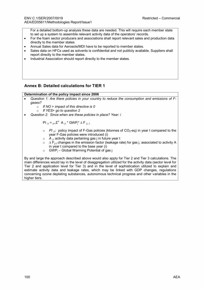
ENV.C.1/SER/2007/0019 Restricted – Commercial AEA/ED05611/Methodologies Report/Issue1
100 AEA
For a detailed bottomup analysis these data are needed. This will require each member state to set up a system to assemble relevant activity data of the operators’ records.
• For the foam sector producers and associations shall report relevant sales and production data directly to the member states
• Annual Sales data for Aerosols/MDI have to be reported to member states. • Sales data on HFCs used as solvents is confidential and not publicly available. Suppliers shall
report directly to the member states. • Industrial Association should report directly to the member states.
Annex B: Detailed calculations for TIER 1
Determination of the policy impact since 2006 • Question 1: Are there policies in your country to reduce the consumption and emissions of F
gases? o If NO > impact of this directive is 0 o If YES> go to question 2
• Question 2: Since when are these policies in place? Year: i
PI i,t = j=1Σ n A j t * GWPj* ∆ F j,i, t
o PI i,t: policy impact of FGas policies (ktonnes of CO2eq) in year t compared to the year FGas policies were introduced (i)
o A j t activity data pertaining gas j in future year t o ∆ Fj,i,t changes in the emission factor (leakage rate) for gas j, associated to activity A
in year t compared to the base year (i) o GWPj – Global Warming Potential of gas j
By and large the approach described above would also apply for Tier 2 and Tier 3 calculations. The main differences would lay in the level of disaggregation utilized for the activity data (sector level for Tier 2 and application level for Tier 3) and in the level of sophistication utilized to explain and estimate activity data and leakage rates, which may be linked with GDP changes, regulations concerning ozone depleting substances, autonomous technical progress and other variables in the higher tiers.

ENV.C.1/SER/2007/0019 Restricted – Commercial AEA/ED05611/Methodologies Report/Issue1
AEA 101
4.11 Guidelines for the Expost impact assessment of ECCP Measures on the Member State level: example for the Emissions Trading Directive
1. Official title of the directive • Directive 2003/87/EC of the European Parliament and of the Council of 13 October 2003
establishing a scheme for greenhouse gas emission allowance trading within the Community and amending Council Directive 96/61/EC
2. Short outline of contents and outline of the directive • Directive 2003/87/EC, commonly known as the ETS Directive, introduces a mandatory capand
trade system for GHGs for the energy sector (power plants, refineries, coke ovens, other combustion installations) and the energyintensive industry (iron & steel, cement, ceramics, pulp & paper). The system is operational since January 1 st 2005. Other sectors and gases can be added, when emissions can be monitored with sufficient certainty. The system is based on direct emissions only, i.e. the ‘stack approach’. The directive governs phase 1 (20052007) and phase 2 (20082012) of the EU ETS. It was revised in December 2008 for the third phase of the ETS.
• For phase 1 and phase 2 individual Member States developed countryspecific National Allocation Plans (NAPs). At the macro level, these NAPs define the cap, i.e. the total quantity of allowances available in each period (ETbudget). Thus, the size of the ETbudget indicates whether the EU ETS is environmentally effective in terms of reducing CO2emissions. At the micro level, NAPs determine how these allowances are allocated to individual installations. By the end of a particular period, operators must surrender the number of allowances equivalent to the amount of emissions caused by their installations during that period. Otherwise sanctions have to be paid. Companies may emit more emissions than their initial allocation if they purchase extra allowances from others. In general, more stringent ETbudgets will lead to higher prices for European Union Allowances (EUAs) and thus greater incentives to improve carbon efficiency, ceteris paribus.
• Operators of installations can buy surplus emission allowances on the market to meet their target. Trading is done in 5year periods, with banking allowed between periods (after an initial 3yr period without banking). JI/CDM credits can be used for compliance within certain (quantitative and qualitative) limits.
• According to the Climate and Energy Package adopted by the EU in 2008, after 2013 the ET budgets and allocation rules will no longer be set by individual Member States, and the third trading period for the ETS will last from 2013 to 2020. The EU intends to reduce total greenhouse gas emissions by 20% compared to 1990 levels. In case other developed countries also decided to take on similar reduction targets within a PostKyoto framework, the EU would commit to a reduction of 30%. To achieve these targets the proposed size of the ETbudget corresponds to a reduction of 21% compared to 2005 emissions for the 20% target, and 38% compared to 2005 emissions for the 30% reduction target. The Climate and Energy Package also includes binding targets for renewables and energy efficiency. By 2020 the target share for renewables in final energy use is 20%. Finally, energy efficiency must be improved by 20% between 2005 and 2020 compared to the business as usual development.
2.1 Relevant reporting requirements under the Directive • All participating installations must monitor their emissions annually in accordance with the EU
Monitoring and Reporting Guidelines. In some countries (depending on transposition into national law monitoring plans need to be approved during permit application). Reports need to be verified by independent third parties.
• Verified emissions are tracked in the registries and the Community Transaction Log (CITL). • Member States must submit a report on the status of implementation on the ETS Directive to
the Commission annually. • If an operator does not meet its monitoring requirements, its trading eligibility is suspended.
ENV.C.1/SER/2007/0019 Restricted – Commercial AEA/ED05611/Methodologies Report/Issue1
102 AEA
3 National policies • Many other Community or national policies affect emissions in the ETS sectors, including:
• Renewable energy policies • Energy efficiency policies • Fuel switch policies • CHP policies • Hosting JI projects
• According to the European Commission allocation under the EU ETS must be consistent with Community legislation and national trends, i.e. installations cannot be allocated more allowances than their emissions would be under Community and national legislation. This means the effect of the EU ETS directive can only be additional to the effects of the other Directives and national policies.
• National emission trading systems – a number of countries had national emission trading systems in place (DK, UK) before the ETS Directive was introduced. These national policies were superseded by the EU ETS in as far as the same sectors/installations were covered.
4. IPCC emission categories affected ETS categories do not match with IPCC emission categories and often only part of the IPCC categories is covered. Also, sector coverage can differ between countries, because of different definitions of ‘combustion installations’ and unilateral optins. In the ETS installations are only covered if they exceed a given threshold in terms of capacity or production (e.g. for combustion installations 20 MW thermal capacity). • 1A1 Fuel Combustion Activities – Energy Industries (CO2, later possibly others) • 1A2 Fuel Combustion Activities Manufacturing Industries and Construction (partly, CO2, later
possibly others) • 1A4 Fuel Combustion Activities – Other Sectors (partly, CO2, later possibly others) • 1A5 Fuel Combustion Activities NonSpecified (CO2, later possibly others) • 2A1. Industrial Processes Cement Production • 2A2. Industrial Processes Lime Production • 2A3. Industrial Processes Limestone and Dolomite Use • 2A4. Industrial Processes Soda Ash Production and Use • 2B2. Chemical Industry Nitric Acid Production (N2O, unilateral optin only) • 2B3. Chemical Industry Adipic Acid Production (N2O, unilateral optin only) Since implementation of the directive (2005), emissions of ETS categories are tracked in the ETS registries and the CITL. 5. Methodological approach 5.1 TIER 1 The Tier 1 approach proposed is based on emission intensity trends and based upon EU wide values:
• Firstly, the sector definition in the Value Added (VA) and emission statistics needs to be matched with the ETS participants. In Tier 1, the correction factors for adjusting the statistics sector definition to match the ETS system boundary (one for sectors, one for gases) are set at 0.
• Secondly, the historic trend in VA and emissions for the appropriate system boundary is determined for the 5 years preceding the implementation of the Directive.
• Thirdly, the historic annual development in emission intensity is assumed to continue in the baseline in absence of the ETS Directive and needs to be combined with the value added in the year of evaluation to determine the baseline emissions.
• Fourthly, the emissions from the baseline must be corrected for the impact of actual energy prices that are different than those occurring in the past. For Tier 1, the correction factor is assumed to be 0 due to data limitations. Such a correction factor could be derived in a future refinement of the methodology from the Tier 3 analysis and applied to the Tier 1/2 approaches
• Fifthly, the effect of the RESE directive on emissions needs to be assessed (as described in the corresponding guideline). The baseline data need to be adjusted to reflect the effect of the RESE directive, by adding the emissions associated with the additional renewable electricity production as determined under the previous step. At the level of Tier 1 it is assumed that all renewables can be associated with targeted RESE policies. A further refined Tier 3 approach may derive in the future factors that could be applied to the Tier 1
ENV.C.1/SER/2007/0019 Restricted – Commercial AEA/ED05611/Methodologies Report/Issue1
AEA 103
approach to correct for impacts of the EU ETS on the deployment of renewables (see the discussion in the Tier 3 report).
• Then, the effect of the ETS Directive is estimated by subtracting the actual verified emissions in the ETS sectors from the corrected baseline data determined in the previous step.
• Finally, the estimated effect of the Directive needs to be corrected for the JI projects hosted in the Member State, by adding the amount of emissions equivalent to the amount of ERUs generated within the Member States from the JI reserve. (Note: This refers to JI projects realised (=hosted) in the respective Member State, not to JI or CDM credits that a Member State purchases from projects realised abroad). Again, at the Tier 1/2 level due to data limitations this correction was not introduced.
Appendix A provides a detailed description of the methodologies described above and details of the calculations performed can be found in appendix B. 5.2 TIER 2 As in TIER 1, except for:
• Correcting the statistics sector definition with a countryspecific correcting factor to match the ETS system boundaries.
• Work at a more disaggregated subsectoral statistical level (especially for the industrial sector)
• Assessing the effect of the RESE Directive according to the Tier 2 approach for that Directive
• Correcting the effect for energy prices that are different from historic trends. 5.3 TIER 3 Evaluation of the EU ETS based on the Tier 3 approach may be conducted using models or carrying out econometric analyses (possibly combined with expert judgements).
a) Evaluation based on models for the power and the industry sectors Models which allow for a sectoral disaggregation of the sectors covered by the EU ETS may be used for evaluation. This approach implicitly assumes that the models are able to capture the actual technological and economic environment, including agents’ behaviour sufficiently well. Models suitable for the task include those capturing several sectors such as the PRIMES model or models for single sectors such as the PowerACE model (a model developed by Fraunhofer ISI for the power sector with an hourly presentation of the power sector). While the former allow for an analysis of the effects on all sectors in all countries combined (including interactions), sectorspecific models with a high resolution in time tend to be better suited to capture technological and countryspecific details including interactions with other policies. In principle, the evaluation consists of the subsequent steps:
Step (i): Run model with observed prices for EUAs in period t and include other economic variables as actually observed in period 1 (energy prices, sector growth, supply of renewables, policies, etc.) as much as possible (without compromising the logic and internal consistency of the model) (Policy run).
Step (ii): Run model from Step (i) but set price for EUAs at zero and – if possible – model counterfactual national climate policy (Counterfactual). The PowerACE and the GreenX models have for this purpose a detailed representation of targeted renewables policies.
Step (iii): Take the difference in emissions between Step (ii) and Step (i) and relate result (e.g. growth rate in emissions) to verified emissions (Calibration).
Due to the long lead times for the planning and construction of new power plants it can be safely assumed that the ETS had no impact on the structure of the power plant portfolio itself in the first period. Therefore the central impact of ETS in the power sector in the first period is the change in plant dispatch caused by higher generation cost for CO2intensive generation technologies. The PowerACE model is capable to simulate plant dispatch on hourly level for an entire year. It applies detailed data on power plants, renewable electricity generation, fuel prices and CO2 prices to calculate plant dispatch, market prices and CO2 emissions. As hourly plant dispatch is crucial for the calculation of emissions in the electricity sector the high detail level is necessary in order to obtain reliable results. In addition the model proceeds through a multiagent

ENV.C.1/SER/2007/0019 Restricted – Commercial AEA/ED05611/Methodologies Report/Issue1
104 AEA
simulation which allows modelling the market behaviour of actors on the electricity markets. At present no models exist at that level of detail at the European level. This is why the impact evaluation with PowerACE is limited to Germany. Models currently used for the exante impact assessment of the EU ETS such as PRIMES are only calculating at fiveyears intervals. In the longer term, investment decisions need to be included in the evaluation. In order to carry out such an integrated analysis it is advisable to combine several models: A plant dispatch model (e.g. PowerACE), a model for the diffusion of renewable electricity generation (e.g. PowerACE RESINVEST or GreenX) and a model the development of the conventional power plant portfolio (e.g. Balmorel,TIMES, MARKAL...). The combination of these model types could provide additional insights into the interaction of renewable support schemes and ETS in different time scales.
b) Econometric approach for the industry sector Using econometric techniques, the EU ETS may be evaluated based on observed (rather than implied or imposed) behaviour. An econometric approach should only be used if sufficient data is available and if the regression equations are well specified. To estimate the savings in emissions associated with the EU ETS, the following adjustment would have to be carried out (for details see the Tier3 report on the EU ETS):
(1) Step (i): adjust for growth rate in sector production (output effect)
(2) Step (ii): adjust for demand reduction in response to increased output prices induced by EU ETS (demandinduced emission reduction effect). In order to improve the methodology in this working step, further work is certainly needed on demand elasticities that show the reaction of the demand for products due to the price of the allowances.
(3) Step (iii): adjust for change in carbon intensity unrelated to policy or input price effects (autonomous technical change effect)
(4) Step (iv): adjust for change in emissions resulting from other policies (policy linkage effect)
(5) Step (v): adjust for change in carbon intensity induced by fuel costs (fuel cost effect)
The direct effects of the EU ETS in the year t may then be quantified by comparing the counterfactual with emissions in the VET. An estimate for the indirect effects of the EU ETS may be obtained by multiplying the change in demand from Step (ii) (in terms of the growth rate) with the counterfactual. 28 It should be pointed out again, when using the econometric approach, particular care needs to be given to the model specification. Findings need to be interpreted in the light of data availability and the quality of econometric results.
Further, since the proposed methodology calculates the direct effects of the EU ETS as a residual, it implicitly assumes that all other mechanism resulting in a reduction of greenhouse gases have been captured. Also, the approach primarily accounts for measures which quickly translate into greenhouse gas emission reductions, in particular fuel switch. The effect of abatement measures which – because of lead times – result in lower future emissions would then also show up as emission savings attributed to the EU ETS in the future. 6. Issue to consider for future evaluations • The EU ETS is a very complex and new instrument. For this reason we would like to highlight
the explorative character of the methodology applied here at the different tier levels and especially the Tier 3 level. It seems to work for the German power sector and the German cement sector; produces “reasonable” results; however, the results depend crucially on some key parameters and assumptions about cost increases, pass through rates, and demand responses. Those parameters need more empirical foundation than they have currently.
• Concerning the power sector the evaluation requires the development of full European models representing on one hand the shortterm dispatching induced by the EU ETS (which requires hourly resolution like in the PowerAce model for Germany and detailed information on the use and characteristics of power plants) and on the other hand the longterm investment effects in the power sector. The interlinkage between targeted renewables and energy policies with the ETS in the Tier 3 approach requires a further discussion process. The outcome of this discussion process could be linked back to the Tier 1 and 2 approaches.
28 If reliable data was available, actual carbon intensity in t may be multiplied by the change in production induced by the demand effect to quantify the demand effect in terms of emissions.
ENV.C.1/SER/2007/0019 Restricted – Commercial AEA/ED05611/Methodologies Report/Issue1
AEA 105
• Concerning the industrial sector a full econometric analysis of the industrial activities as described in the Tier 3 report for the EU ETS is necessary. It is further necessary, to conduct misspecification tests to assess the appropriateness of the underlying econometric model from a statistical perspective. Although regressions test have been carried out, see Tier 3 report, results are to be considered as exemplary and could be improved further when longer time periods are available in the future from the allowance registries. Other methodological approaches may also be further explored: given the experience to be gained with the evaluation of the EU ETS a diversity of approaches may be explored to better understand sensitivities in the methodologies used and the underlying data requirements.
• The issue of CDM/JI projects interacting with the EU ETS needs to be further explored. In the current approach it is assumed that in absence of JI projects, the corresponding emission reductions would not have taken place in the EU ETS. In part, however, the emission reduction measures comprising the JI project could also be incentivised by the carbon price instituted by the EU allowance price. The extent to which this occurs will depend on the differential in the EU allowance price and the ERU price and the period over which that differential is (expected to be) maintained. This effect is not taken into account here. In the discussion process for the development of the methodology the argument was advanced that the impacts of CDM and JI should also be attributed to EU ETS, even if they take place elsewhere. In our view this is too far reaching an interpretation of the flexibility instrument ETS by allocating the impacts of the CDM to the ETS. This is seen by the fact that CDM may be used by countries that have no ETS. This clearly shows that the CDM is an instrument per se. The question would then be rather in how far the ETS by its presence enhances the uptake of CDM projects. Further discussion of the issue is certainly necessary.
• In case further sectors and gases are added to the system (N2O for some processes is already envisaged for some industrial processes), additional steps in the methodology may be needed, especially in terms of data sources and system boundaries (e.g. aviation or shipping).
• When domestic offset projects become feasible within the scheme, additional steps in the methodology will be needed, adding the effects of domestic offset projects on emissions in non ETS sectors to the estimated effect of the ETS Directive.
ENV.C.1/SER/2007/0019 Restricted – Commercial AEA/ED05611/Methodologies Report/Issue1
106 AEA
4.11.1 Annex A: Explanations for main methodological assumptions
6.1 Determination of the policy impact since 1990
Step 1: Given the large number of policies that influence the emissions in the sectors and installations covered by the EU ETS, it is not possible to define the impact of individual policies since 1990. Policy sets will also differ by Member State and the starting date of the various policies will be different.
Step 2: The impact of the set of policies is combined into the baseline emissions (at 0 carbon price) in the autonomous emission intensity improvement (Tier 1/2) or the modelbased approach (Tier 3).
Tier 1/2 Approach: The carbon intensity of an economy (CO2 or greenhouse gas emissions per unit of GDP) or a sector (CO2 or GHG emissions per unit of value added) is the resultant of the energy efficiency, the fuel mix and the economic structure (or product mix at the sector level). All of these will change over time, a development that can be further influenced by (energy prices and) a carbon price. The historic trend in carbon intensity – over the 5yr period before the introduction of the carbon price – as measured in annual % change in CO2 (or GHG)/VA for the appropriate sectors will be the basis for determining the baseline emissions. The annual change will be applied over the period that the Directive has been active until the year of evaluation, and combined with actual value added in the appropriate sectors to establish the baseline emissions in the year of evaluation. Note that fixedyear currencies (e.g. 1998Euro) must be used in this assessment to account for inflation. Use market exchange rates if necessary. Note that part of the installations included in the EU ETS takes place in socalled ‘nonproductive’ sectors, i.e. sectors that do not generate value added. This is mainly the case for the own generation of heat and/or electricity in smaller, onsite combustion installations in large buildings in the tertiary sector (hospitals, universities, large governmental buildings). Data on the sector in which combustion installations are located are often not available. However, the sectoral definitions used in both emission and value added statistics means both the emissions and value added of these installations are not included, i.e. this issue can be ignored.
Tier 3 Approach: The emissions in the appropriate sectors according to the most recent PRIMES scenario with a 0 carbon price are selected as the baseline emissions in this approach. Note that some countries, e.g. the UK and Denmark, had a national emission trading system in place before the EU ETS Directive was introduced, in which a carbon price existed. Since these systems were either abolished before or replaced by the introduction of the EU ETS, their effect is ignored here.
Step 2: Included in the ETS are participants over a certain size threshold in the:
• Iron & steel sector • Cement sector • Glass sector • Ceramics sector • Pulp & paper sector • Refinery sector • Cokes production • Combustion installations, including public and private sector electricity and heat plants, but
also other combustion installations, processintegrated and furnaces, especially in the chemical industry and the food industry, but even spread throughout the tertiary sector
This means that sector definitions in models and/or statistics will cover a larger share of plants than included in the ETS for most sectors, although for the category of combustion installations the opposite may occur.
In Tier 1, we assume the correction factor to be 0, i.e. the corresponding sectors are assumed to

ENV.C.1/SER/2007/0019 Restricted – Commercial AEA/ED05611/Methodologies Report/Issue1
AEA 107
match. In this case, the sectors most likely to be included (depending on aggregation level available) are:
• Iron & steel • Building materials • Pulp & paper • Energy • (refineries might be distinguished separately) • (coke plants may be mentioned separately or covered under the iron & steel sector)
Step 3: Energy prices can influence GHG emissions by changing the profitability of emission reduction measures and by changing priorities in agendasetting. If energy prices assumed in historic trends (Tier 1/2) or modelling baseline scenarios (Tier 3) is significantly different from actual energy prices during the time of the evaluation, the baseline will not represent the development in absence of the Directive. Therefore, the effect of the Directive will be overestimated (in case real energy prices are higher than assumed in the baseline) or underestimated (in case real energy prices are lower than assumed in the baseline). Therefore, the baseline emissions need to be corrected for the impact of differences in energy prices. The correction needs to take into account inflation and purchasing power parities. In Tier 1/2, no correction factor is applied.
Step 4: Allocation under the ETS must be ‘consistent with Community legislation’, meaning that participants cannot be allocated more than what they would need if all Community legislation is met. Specifically in relation to the RESE Directive, the Commission has emphasised that efforts in the ETS must be additional to the efforts resulting from the targets under the RESE Directive. Therefore, emission reductions observed in the EU ETS sectors that are attributable to the RESE Directive cannot be attributed to the EU ETS. We assume all RESE derived emission reductions to overlap with the EU ETS, as long as the country targets in the RESE Directive are not yet met. Emission reductions resulting from renewable electricity production over and above the targets in the RESE Directive do not need to be corrected for. Note that in some cases, renewable electricity could replace electricity produced by small installations (e.g. boilers) not covered by the EU ETS (< 20MW, taking into account the aggregation rule). In this case, the resulting emission reductions would not be observed in the actual emission data for the EU ETS sectors, i.e. the actual EU ETS emissions should not be corrected for the overlap. However, in general no data are available on the distribution of the size of electricity generators, especially in this small end of the range. Therefore, this cannot be taken into account.
6.2 Determination of the policy impact since the directive is in force.
Step 1: The Directive is in place as of 1 st of January 2005, except for Member States that entered the EU at a later stage. In this case, the Directive is considered to be in force from the beginning of the 1 st year in which the Member State participates in the trading regime, as agreed by the Commission.
Step 2: The sum of the verified emissions of the individual ETS participants as reported in the CITL represents the actual emissions in the EU ETS sectors after implementation of the Directive.
Step 3: The effect of the ETS Directive is estimated by subtracting the actual ETS emissions as determined in the previous step from the corrected baseline emissions, as determined in step 4 described in Section 6.1.
Step 4: The actual emissions in the EU ETS sector will be lower in case the Member State hosts JI projects in sectors that reduce the emissions in the ETS sectors, and that would also have occurred in the absence of the EU ETS Directive. Note that this does not only refer to JI projects IN ETS sectors (direct effect), but also JI projects in other sectors that influence emissions in the EU ETS sectors, i.e. stand alone renewable electricity generation or standalone smallscale heat generation, that reduce the demand from electricity or heat plants covered by the EU ETS (indirect effect, as per the

ENV.C.1/SER/2007/0019 Restricted – Commercial AEA/ED05611/Methodologies Report/Issue1
108 AEA
Commission’s ‘Doublecounting Decision’). The estimated effect of the ETS Directive therefore needs to be corrected for the effect of a part of the JI projects. The emission credits for both direct and indirect JI projects as included in the JI reserve (during Phase II), and need to be reported to the Commission. However, in case the overlapping JI projects produce renewable electricity, the correction has already been included in the correction of the baseline for RESE generation, and no further correction should be made in this case. In other words, the correction for JI projects should only be made for JI projects that do not produce renewable electricity. Note that the correction of actual EU ETS emissions for JI projects assumes that in absence of JI projects the emission reduction measures comprising the JI projects would not be taken as a consequence of the EU allowance price. 6.3 Uncertainty analysis The main uncertainty arises in: • The inconsistency of sector boundaries between ETS/nonETS participants and boundaries
distinguished in modelling/statistics • The lack of empirical basis for elasticities to estimate demand reduction effects in the industrial
sector or the passthough factors for electricity prices and industrial products. • The effect of changing energy prices • The effect of other factors driving carbon intensity over time, which change during the period
used for establishing the historic trend or the evaluation period. 6.4 Data sources • PRIMES scenarios • Eurostat statistics on value added and emissions • CITL verified emissions from the EU ETS • Data sources needed for estimating the effect of the RESE directive (as described in the
Guideline for evaluation the effect of that Directive) • Reports submitted in the context of the Doublecounting Decision
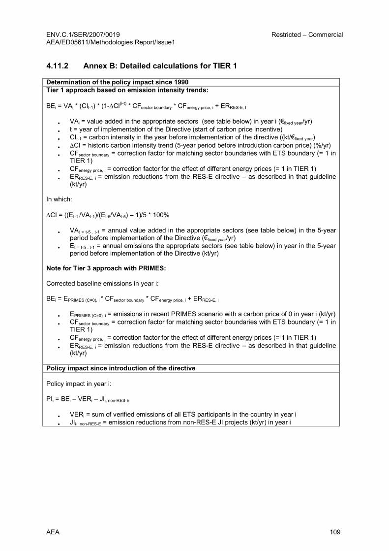
ENV.C.1/SER/2007/0019 Restricted – Commercial AEA/ED05611/Methodologies Report/Issue1
AEA 109
4.11.2 Annex B: Detailed calculations for TIER 1
Determination of the policy impact since 1990 Tier 1 approach based on emission intensity trends:
BEi = VAi * (CIt1) * (1∆CI (it) * CFsector boundary * CFenergy price, i + ERRESE, I
• VAi = value added in the appropriate sectors (see table below) in year i (€fixed year/yr) • t = year of implementation of the Directive (start of carbon price incentive) • CIt1 = carbon intensity in the year before implementation of the directive ((kt/€fixed year) • ∆CI = historic carbon intensity trend (5year period before introduction carbon price) (%/yr) • CFsector boundary = correction factor for matching sector boundaries with ETS boundary (= 1 in
TIER 1) • CFenergy price, i = correction factor for the effect of different energy prices (= 1 in TIER 1) • ERRESE, i = emission reductions from the RESE directive – as described in that guideline
(kt/yr)
In which:
∆CI = ((Et1 /VAt1)/(Et5/VAt5) – 1)/5 * 100%
• VAt = t5 ..t1 = annual value added in the appropriate sectors (see table below) in the 5year period before implementation of the Directive (€fixed year/yr)
• Et = t5 ..t1 = annual emissions the appropriate sectors (see table below) in year in the 5year period before implementation of the Directive (kt/yr)
Note for Tier 3 approach with PRIMES:
Corrected baseline emissions in year i:
BEi = EPRIMES (C=0), i * CFsector boundary * CFenergy price, i + ERRESE, i
• EPRIMES (C=0), i = emissions in recent PRIMES scenario with a carbon price of 0 in year i (kt/yr) • CFsector boundary = correction factor for matching sector boundaries with ETS boundary (= 1 in
TIER 1) • CFenergy price, i = correction factor for the effect of different energy prices (= 1 in TIER 1) • ERRESE, i = emission reductions from the RESE directive – as described in that guideline
(kt/yr)
Policy impact since introduction of the directive
Policy impact in year i:
PIi = BEi – VERi – JIi, nonRESE
• VERi = sum of verified emissions of all ETS participants in the country in year i • JIi, nonRESE = emission reductions from nonRESE JI projects (kt/yr) in year i

ENV.C.1/SER/2007/0019 Restricted – Commercial AEA/ED05611/Methodologies Report/Issue1
110 AEA
4.12 Guidelines for the Expost impact assessment of ECCP Measures on the Member State level: example for the Energy Performance of Buildings Directive
1. Official title of the directive • Directive on the energy performance of buildings (2002/91/EC) 2. Short outline of contents and outline of the directive • In 2002 the Buildings Directive was adopted and is aimed at influencing energy losses through
the building shell, and for the service sector also includes air conditioning and lighting. Among others this directive obliges Member States to introduce minimum efficiency standards for existing, renovated and new residential and service buildings, introduce a labelling system for existing buildings, set up a system for regular boiler and air conditioning inspection.
• The directive came into force in 2002. Member States were required to bring into force the laws, regulations and administrative provisions necessary to comply with the Directive at the latest on 4 January 2006. However 3 year delays are permitted if a MS lacks the necessary experts. Many countries make use of this transition period due to implementation problems such as building certification schemes or the regular inspection.
3. National policies • Already before the introduction of the EPBD a large variety of energy efficiency policies are (or
have been) in place to stimulate energy savings in the built environment. First policies were introduced during the oil crises in the 1970s and 1980s. A lot of Member States already had minimum efficiency standards in place for new buildings. For existing buildings focus was mainly on financial incentives and voluntary agreements.
4. IPPC emission categories affected • 1A1a Fuel Combustion Activities – Energy Industries – Public Electricity and Heat Production
(relevant for electric heating and district heating) • 1A4 Fuel Combustion Activities – Other Sectors (CO2, N2O, CH4) (main sector of impact) • 1A5 Fuel Combustion Activities NonSpecified (CO2, N2O, CH4) 5. Methodological approach 5.1 TIER 1 • Tier 1 assumes a simple linear relation for the residential sector between the total number of
residential buildings and the level of greenhouse gas emissions. I.e. in the absence of policies greenhouse gas emission in principle increase in the same pace as the total number of residential buildings.
• Tier 1 assumes a simple linear relation for the service sector between the total number of employees and the level of greenhouse gas emissions. I.e. in the absence of policies greenhouse gas emission increase in the same pace as the total number of employees. The choice to take the total number of employees as an indication for energy use in the service sector is a pragmatic one. This is the number which is readily available for most member states and mostly updated on an annual basis.
• Various studies 29 have shown that energy efficiency measures in the built environment are, and have been costeffective from the perspective of the enduser of a building. This means that in the absence of policies efficiency improvements in the built environment would have taken place as well. “Autonomous” technological developments (new buildings are more efficient than old buildings) and the fact that a lot of energy saving measures are economical contribute to this efficiency improvement. In the Tier 1 approach we take the approach that in case policies have been in place (see question 1 to 4), all savings that go beyond 0.5% autonomous efficiency improvement per year can be considered as the impact of policies which is a rate derived from the 19902002 period.
• Tier 1 approach applies the IPCC default CO2 emission factor per type of fuel. • Tier 1 approach assumes that renewable electricity production is replacing the average
European fuel mix of the EU27 of public and autoproducers • Tier 1 approach assumes that share of energy use for space heating is unchanged over the
years, and uses default values per country (see table on following page)
29 E.g. see Ecofys studies for Eurima, and the Sectoral Objectives study. McKinsey (2007). Fraunhofer (2007 and 2008)
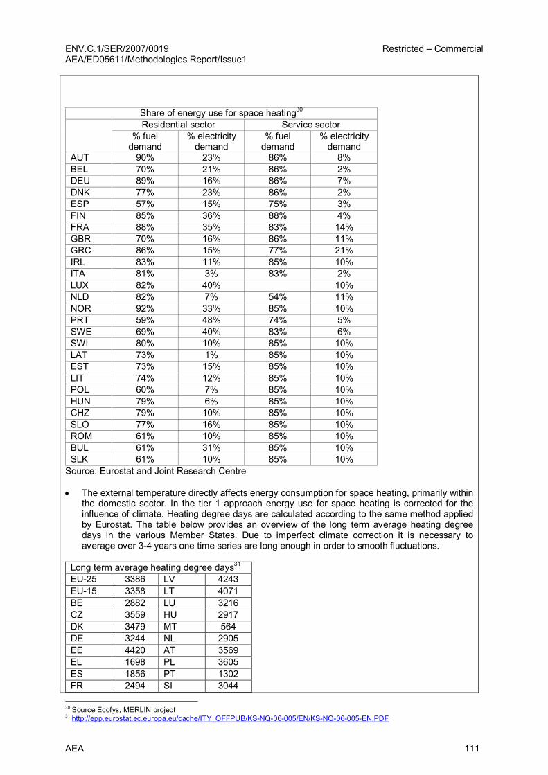
ENV.C.1/SER/2007/0019 Restricted – Commercial AEA/ED05611/Methodologies Report/Issue1
AEA 111
Share of energy use for space heating 30
Residential sector Service sector % fuel demand
% electricity demand
% fuel demand
% electricity demand
AUT 90% 23% 86% 8% BEL 70% 21% 86% 2% DEU 89% 16% 86% 7% DNK 77% 23% 86% 2% ESP 57% 15% 75% 3% FIN 85% 36% 88% 4% FRA 88% 35% 83% 14% GBR 70% 16% 86% 11% GRC 86% 15% 77% 21% IRL 83% 11% 85% 10% ITA 81% 3% 83% 2% LUX 82% 40% 10% NLD 82% 7% 54% 11% NOR 92% 33% 85% 10% PRT 59% 48% 74% 5% SWE 69% 40% 83% 6% SWI 80% 10% 85% 10% LAT 73% 1% 85% 10% EST 73% 15% 85% 10% LIT 74% 12% 85% 10% POL 60% 7% 85% 10% HUN 79% 6% 85% 10% CHZ 79% 10% 85% 10% SLO 77% 16% 85% 10% ROM 61% 10% 85% 10% BUL 61% 31% 85% 10% SLK 61% 10% 85% 10% Source: Eurostat and Joint Research Centre
• The external temperature directly affects energy consumption for space heating, primarily within the domestic sector. In the tier 1 approach energy use for space heating is corrected for the influence of climate. Heating degree days are calculated according to the same method applied by Eurostat. The table below provides an overview of the long term average heating degree days in the various Member States. Due to imperfect climate correction it is necessary to average over 34 years one time series are long enough in order to smooth fluctuations.
Long term average heating degree days 31
EU25 3386 LV 4243 EU15 3358 LT 4071 BE 2882 LU 3216 CZ 3559 HU 2917 DK 3479 MT 564 DE 3244 NL 2905 EE 4420 AT 3569 EL 1698 PL 3605 ES 1856 PT 1302 FR 2494 SI 3044
30 Source Ecofys, MERLIN project 31 http://epp.eurostat.ec.europa.eu/cache/ITY_OFFPUB/KSNQ06005/EN/KSNQ06005EN.PDF
ENV.C.1/SER/2007/0019 Restricted – Commercial AEA/ED05611/Methodologies Report/Issue1
112 AEA
IE 2916 SK 3440 IT 2085 SE 5423 CY 787 UK 3354 Source: Eurostat and Joint Research Centre 5.2 TIER 2 • Same as tier 1 but is based on m2 in both the residential and service sector buildings rather
than the number of dwellings and assumes that saved electricity would have been produced by the average national fuel mix for the power production in a country (fossil, nuclear plus renewable public as well as autoproducers).
5.3 TIER 3 • The Tier 3 approach tries to determine the autonomous deployment of energy efficiency
measures in the building sector applying a bottomup approach (MURE simulation model) in which the costeffectiveness of individual measures is analysed. This means that:
o the Tier 3 includes an overview of energy savings measures that have been implemented per building category (implementation degree, savings per building costs).
o The Tier 3 includes a calculation on the energy savings measures that were cost effective (“autonomous savings”) and the saving that were not costeffective (policy induced measures). Thus the impact of energy prices are taken into account
o It simulates explicitly the penetration of buildings into the stock and provides thus an estimate for the autonomous progress due to previous regulation.
o It makes assumptions about noncompliance with building regulations. • Tier 3 assumes a start of the impacts only after 2006 at the earliest. • Tier 3 includes a further detailing for the residential sector with respect to the various types of
residential buildings (single/multifamily buildings). Tier 3 assumes a linear relation between the m 2 of heated space per category and the level of greenhouse gas emissions.
• Tier 3 includes in principle a further detailing for the service sector with respect to the various types of service buildings. However, due to data limitations this approach cannot be followed up to a sufficient degree of detail. Tier 3 assumes a linear relation between the total floor surface per category and the level of greenhouse gas emissions.
• Tier 3 applies a country specific fuel mix to determine CO2 impact of the savings. Emission factors for saved electric are based on short term marginal emissions per MS.
6. Detailed elaboration of TIER 1 approach 6.1 Determination of the policy impact
• Question 1: Are there policies in place in your country to stimulate energy efficiency improvement in the residential sector?
o If NO > impact of directive for the residential sector is 0 o If YES> go to question 2
• Question 2: Since when are these policies in place? Year: i
• Question 3: Are there policies in place in your country to stimulate energy efficiency improvement in the service sector?
o If NO > impact of this directive is 0 o If YES> go to question 4
• Question 4: Since when are these policies in place? Year: i
• Policy impact in year t since the introduction of policies (year i) for the residential sector:
PIi,t = (((10.5%)^ (ti) Ei) – Et) * Ft * At
o The year 2002 is used as a default as the starting year. o PIi,t policy impact of energy efficiency policies in the residential sector (ktonnes of CO2
eq) in year t compared to the year policies were introduced year i o At number of households in year t o Ei final temperature corrected energy consumption for space heating per household in
the year policies were introduced (year i) o Et final temperature corrected energy consumption for space heating per household in
year t
ENV.C.1/SER/2007/0019 Restricted – Commercial AEA/ED05611/Methodologies Report/Issue1
AEA 113
o Ft carbon intensity for the energy consumption in the household sector in year t
• Ei calculation of final temperature corrected energy consumption for space heating per household in year i:
o Take the default factor on the share of energy use for space heating for your country for fuel use in the residential sector (Sf) and for electricity (Se)
o Determine the fuel consumption for the household sector in year i (FCi): Coal consumption in year i + Natural gas consumption in year i + Oil consumption in year i (TJ) + renewables consumption in year i.
o Determine the electricity consumption for the household sector in year t (ECi). o Determine the number of households in year Ai o Determine the correction factor for temperature fluctuations by taking the long term
average heating degree days (Tl) and the actual heating degree days (Tai) in year i.
Ei = [(FCi * Sf + ECi * Se) * (Tl/Tai)]/Ai
• Et calculation of final temperature corrected energy consumption for space heating per household in year t (GJ/household). Same calculation procedure as for Ei
• Ft calculation of the carbon intensity for the energy consumption in the household sector in year t:
o [Coal consumption in year t* CO2 emission factor for coal + Natural gas consumption in year t * CO2 emission factor for natural gas (kton/PJ) + Oil consumption in year t * CO2 emission factor for oil (kton/PJ) (TJ) + electricity consumption in year t * EU27 average emission factor for electricity production] divided by
o FCt+ECt
• Policy impact in year t since the introduction of policies (year i) for the service sector is calculated using the same calculation rules as for the residential sector. For the service sector:
o Activity indicator is the number of employees o Share of energy use for space heating differs from the residential sector
6.2 Uncertainty analysis • Uncertainty in the numbers on the share of energy used for space heating in the residential and
service sector. These numbers are not regularly updated. • Uncertainty is related to the uncertainly in the energy statistics used, and the use of default
emission factors • Energy statistics on the service sector are usually not of a very high quality and includes
relatively large uncertainties • Assumption with respect to autonomous efficiency improvement of 0.5% per year in the
residential sector and 0% per year for the service sector. This is derived from the period 1990 2002 and needs to be revised or quantitative evidence provided to support the assumption.
• National policies are at varying levels of implementation and reductions may not have occurred as a result of the Directive to date.
• Whether or not comfort factors are to be included in the analysis (difference between Tier 1 and 2) introduces major differences in the results as long as comfort is increasing in the buildings.
6.3 Data sources • Actual heating degree days: JRC • Default emission factors for fossil fuel: http://www.ipcc
nggip.iges.or.jp/public/2006gl/pdf/2_Volume2/V2_2_Ch2_Stationary_Combustion.pdf (Table 2.2)
• Eurostat: Electricity and energy statistics • Eurostat: Household statistics • Eurostat: Employment statistics 7. Issue to consider for future evaluations • More recent data on the split of energy use in the household sector into various functions:
space heating, hot water production, cooling, lighting etc. • Improved data basis for the service sector energy uses • Noncompliance with building regulation • Data averaging for the Tier 1 and 2 approaches which is necessary due to imperfect corrections

ENV.C.1/SER/2007/0019 Restricted – Commercial AEA/ED05611/Methodologies Report/Issue1
114 AEA
for climatic variations • Eurostat’s focus to move from final energy consumption to primary. After the heating surveys
cooling surveys are the next stage in the process.

ENV.C.1/SER/2007/0019 Restricted – Commercial AEA/ED05611/Methodologies Report/Issue1
AEA 115
4.13 Guidelines for the Expost impact assessment of ECCP Measures on the Member State level: example for the Labelling of household appliances
1. Official title of the directive • COUNCIL DIRECTIVE 92/75/EEC of 22 September 1992 on the indication by labelling and
standard product information of the consumption of energy and other resources by household appliances.
• Implementation directives for each household appliance: • 2003/66/EC, amending directive 1994/2/EC, household electric refrigerators freezers
and combinations thereof • 2002/40/EC, electric ovens • 2002/31/EC, household air conditioners • 1999/9/EC, amending directive 1997/17/EC, household dishwashers • 1998/11/EC, household lamps • 1997/17/EC, household dishwashers • 1996/89/EC, amending directive 1995/12/EC, household washing machines • 1996/60/EC, combined washer drier • 1996/57/EC, household electric refrigerators freezers and combinations thereof • 1995/13/EC, household electric tumble driers • 1995/12/EC, household washing machines
2. Short outline of contents and outline of the directive • The directive introduces a common format for the labelling of energy consumption information
concerning household appliances such as refrigerators, freezers and their combinations, washing machines, driers and their combinations, dishwashers, ovens, water heaters and hot water storage appliances, lighting sources, airconditioning appliances
• Details relating to the label and the fiche were defined by several directives, each relating to different types of appliances
2.1 Relevant reporting requirements under the Directive • Member States are required to communicate to the Commission about the main provisions of
domestic law which they adopt in the field covered by this Directive 3 Policy Interaction 3.1 EU Policies The main area where there may be an interaction with labelling directives is in relation to those on minimum standards (e.g. 1996/57/EC on cold appliances), voluntary agreements with manufacturers on a wider range of household products as well as potential future minimum standards under Directive 2005/32/EC establishing a framework for the setting of ecodesign requirements for energyusing products.
IMPLICATIONS: In practice minimum efficiency performance standards (MEPS) act to limit the lowest efficiency performance of the bottom of the appliance market whereas the impact of labelling seeks to drive the speed of penetration of the highest performing, section of the market. Hence in this case the impact of labelling can be assumed to be differentiable with minimal policy interaction. Also MEPS have only been introduced for cold appliances so far, and relatively late compared to the impact of the Labelling Directive. De facto the less efficient cold appliances had already disappeared when the MEPS took effect.
Other impacts on the penetration of more efficient appliances may, for example, be driven by incentives for efficient procurement (e.g. via the need for the public sector to demonstrate a leading role under the Energy Services Directive 2006/32/EC). However, this is primarily concerned with nondomestic appliances and so is not applicable here. 3.2 National Policies • Prior to the introduction of the directive appliance labelling had been introduced in France and
West Germany. Denmark and the Netherlands had proposed a labelling system but had not
ENV.C.1/SER/2007/0019 Restricted – Commercial AEA/ED05611/Methodologies Report/Issue1
116 AEA
implemented it • The timing of implementation of the different directives, varied by country. • At the national level there may also be schemes which actively incentivise the uptake of new
products (e.g. elements of the UK Energy Efficiency Commitment and earlier Energy Efficiency Standards of Performance Scheme).
IMPLICATIONS: In the case of national labelling or incentivising schemes there is a direct overlap between the impact of the label and other policy drivers on uptake, which it will not be possible to distinguish under a Tier 1 or 2 approach). However, in the situation of an earlier national scheme for labelling, the savings from EU labelling should potentially be discounted. 4. IPPC emission categories affected Indirect GHG emissions deriving from electricity use • 1A4 Fuel Combustion Activities – Other Sectors (CO2, N2O, CH4) • 1A5 Fuel Combustion Activities NonSpecified (CO2, N2O, CH4) 5. Methodological approach 5.1 TIER 1 Currently no EU official statistical data (Eurostat/inventory/registry) are available for the energy used by household appliances, for the energy efficiency characteristics of household appliances sold in the market and for the number of household appliances sold in a given year. Consequently a tier 1 approach is only applicable on a more aggregate level for this directive, e.g. on the level of overall residential energy consumption per dwelling.
If better data were available on the energy performance of new appliances sold in the EU, and on their energy use, a basic Tier 1 approach would become feasible. A tier 1 approach would: • assume that the provision of energy use information to potential buyers of appliances leads to
an increased market share for higher efficiency appliances. • assume that the total number of appliances sold in each year is not affected by the directive • assume that the impact of regulations mandating energy efficiency standards (when present)
would be independent from the impact of the labelling system • not consider autonomous development (i.e. frozen efficiency) and structural change – i.e. in
absence of the directive the energy efficiency of household appliances would have remained constant
• not consider the potential impact of other variables that could potentially affect consumers’ behaviour (such as appliances prices, buyers’ income, number of household components, dwellings average size)
• assume a simple linear relation between increase in appliances efficiency and decrease in electricity use (i.e. increased efficiency does not lead users to increase use – such that there is no rebound effect)
• assume that the average annual usage of appliances is the same in each member state. • only determine the impact of energy efficiency improvements in appliances on CO2 emissions • assume that a reduction in electricity use leads to a reduction in electricity production that
matches the average power plant to be used in EU27.
Based on these assumptions the tier 1 approach would calculate the impact of the directive by estimating, appliance per appliance, the difference in yearly electricity use of new appliances with and without the directive and considering the total number of appliances sold each year to assess the total impact of the directive. However, this approach will also include the impact of any national incentivising policies on the uptake of more efficient appliances.
ENV.C.1/SER/2007/0019 Restricted – Commercial AEA/ED05611/Methodologies Report/Issue1
AEA 117
5.2 TIER 2 Tier 2 makes use of EU official and unofficial data, as well as MS data mainly of those collected at the level of the Odyssee project for energy efficiency indicators (www.odysseeindicators.org). The Tier 2 approach shares a number of characteristics with Tier 1, such as assuming that: • the provision of energy use information to potential buyers of appliances leads to an increased
market share for higher efficiency appliances. The rating above which the label is assumed to have an impact will be specified for each appliance (for example B or above, as opposed to D or above).
• the total number of appliances sold in each year is not affected by the directive • the impact of regulations mandating energy efficiency standards (when present) is independent
from the impact of the labelling system • it is assumed that overall the potential impact of other variables that could potentially affect
consumers’ behaviour (such as appliances prices, buyers’ income, number of household components, dwellings average size) is negligible
• It is further assumed that an increase in appliances efficiency will linearly lead to a decrease in electricity use (i.e. increased efficiency does not lead users to increase use – such that there is no rebound effect)
• Tier 2 only determines the impact of energy efficiency improvements in appliances on CO2 emissions
Additionally Tier 2 • differentiates the annual energy consumption of different appliances in different Member States
as this will impact directly on the absolute level of savings for a more efficient appliance. For example, greater use of air conditioners in more Southerly countries.
• Differentiates the autonomous energy efficiency improvement by Member State (however, based on the real data which are not available for all countries and all appliances, this appears as difficult at present)
• Assumes that reduction in energy use deriving from the increase in energy efficiency is replacing the average plant for a specific Member State.
Based on these assumptions the Tier 2 approach calculates the impact of the directive by estimating, appliance per appliance and country by country, the difference in yearly electricity use of new appliances with and without the directive and considering the total number of appliances sold each year to assess the total impact of the directive. As per Tier 1 this will still include the impact of any national incentivisation policies as well as the Directive itself.
5.3 TIER 3 The tier 3 approach • is based on a stock model for the different electric appliances and uses the split of labelling
classes as an input • models and determines the autonomous development of energy efficiency in appliances,
derived from periods previous to the policy and/or expert judgement • seeks to determine the impact of a broader set of socioeconomy factors (appliances prices,
electricity prices, income, household size, dwelling size) on consumers’ behaviour. Currently. Date on these issue are, however, limited.
• seeks to determine the impact that the availability of more efficient appliances may have on consumers’ behaviour (rebound effect)
• seeks to understand potential differences in appliance usage and appliance size across MSs in the determination of energy savings
• seeks to separate the impact of national incentivisation policies on the uptake of more efficient appliances
• determines the impact of reduced electricity use on CO2, N2O, and CH4
• assumes that a reduction in electricity use leads to a reduction in the national marginal production of public and auto producers
6. Issue to consider for future evaluations • Sourcing relevant data (e.g. historic data on the energy efficiency of appliances, data on new
appliances sold and their energy efficiency score, actual appliance usage in households, etc.) constitutes a key issue when determining the impact of this directive – or of any other directive

ENV.C.1/SER/2007/0019 Restricted – Commercial AEA/ED05611/Methodologies Report/Issue1
118 AEA
that affects energy consumption of appliances. The Odyssee database is starting to collect some of the relevant information on these markets but the best data sources currently available on the appliances markets remain private sector market research companies (for example GfK). Long term solutions to fix data gaps will have to be considered.
• As new directives come into force or are fully implemented (such as the Ecodesign directive) they will also impact energy use of new appliances. This will increasingly take up the impacts of Council Directive 92/75/EEC
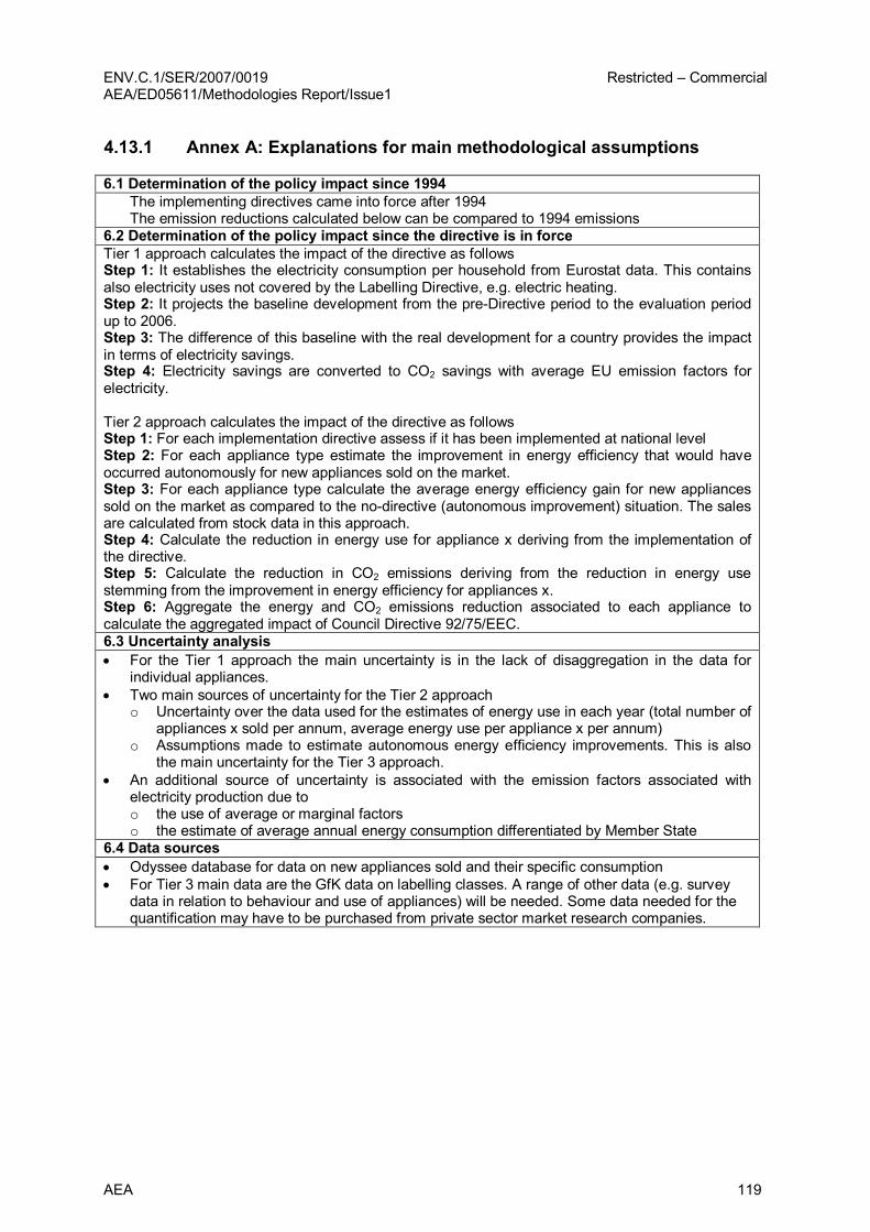
ENV.C.1/SER/2007/0019 Restricted – Commercial AEA/ED05611/Methodologies Report/Issue1
AEA 119
4.13.1 Annex A: Explanations for main methodological assumptions
6.1 Determination of the policy impact since 1994 The implementing directives came into force after 1994 The emission reductions calculated below can be compared to 1994 emissions
6.2 Determination of the policy impact since the directive is in force Tier 1 approach calculates the impact of the directive as follows Step 1: It establishes the electricity consumption per household from Eurostat data. This contains also electricity uses not covered by the Labelling Directive, e.g. electric heating. Step 2: It projects the baseline development from the preDirective period to the evaluation period up to 2006. Step 3: The difference of this baseline with the real development for a country provides the impact in terms of electricity savings. Step 4: Electricity savings are converted to CO2 savings with average EU emission factors for electricity.
Tier 2 approach calculates the impact of the directive as follows Step 1: For each implementation directive assess if it has been implemented at national level Step 2: For each appliance type estimate the improvement in energy efficiency that would have occurred autonomously for new appliances sold on the market. Step 3: For each appliance type calculate the average energy efficiency gain for new appliances sold on the market as compared to the nodirective (autonomous improvement) situation. The sales are calculated from stock data in this approach. Step 4: Calculate the reduction in energy use for appliance x deriving from the implementation of the directive. Step 5: Calculate the reduction in CO2 emissions deriving from the reduction in energy use stemming from the improvement in energy efficiency for appliances x. Step 6: Aggregate the energy and CO2 emissions reduction associated to each appliance to calculate the aggregated impact of Council Directive 92/75/EEC. 6.3 Uncertainty analysis • For the Tier 1 approach the main uncertainty is in the lack of disaggregation in the data for
individual appliances. • Two main sources of uncertainty for the Tier 2 approach
o Uncertainty over the data used for the estimates of energy use in each year (total number of appliances x sold per annum, average energy use per appliance x per annum)
o Assumptions made to estimate autonomous energy efficiency improvements. This is also the main uncertainty for the Tier 3 approach.
• An additional source of uncertainty is associated with the emission factors associated with electricity production due to o the use of average or marginal factors o the estimate of average annual energy consumption differentiated by Member State
6.4 Data sources • Odyssee database for data on new appliances sold and their specific consumption • For Tier 3 main data are the GfK data on labelling classes. A range of other data (e.g. survey
data in relation to behaviour and use of appliances) will be needed. Some data needed for the quantification may have to be purchased from private sector market research companies.
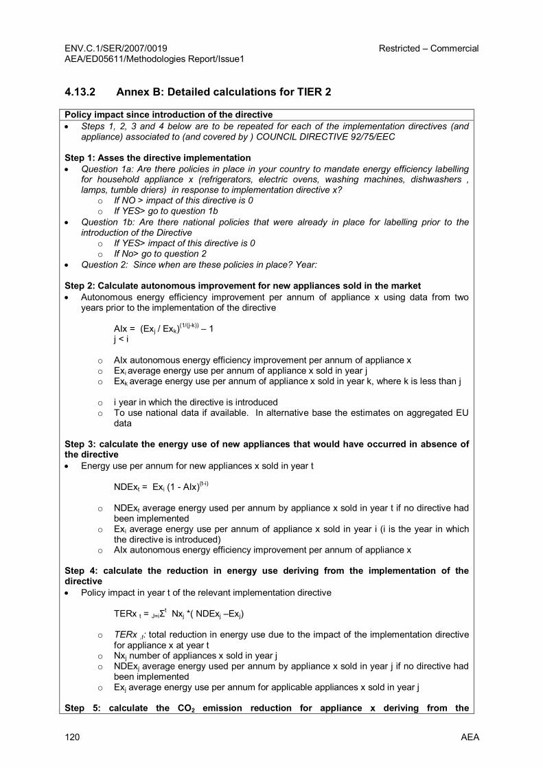
ENV.C.1/SER/2007/0019 Restricted – Commercial AEA/ED05611/Methodologies Report/Issue1
120 AEA
4.13.2 Annex B: Detailed calculations for TIER 2
Policy impact since introduction of the directive • Steps 1, 2, 3 and 4 below are to be repeated for each of the implementation directives (and
appliance) associated to (and covered by ) COUNCIL DIRECTIVE 92/75/EEC
Step 1: Asses the directive implementation • Question 1a: Are there policies in place in your country to mandate energy efficiency labelling
for household appliance x (refrigerators, electric ovens, washing machines, dishwashers , lamps, tumble driers) in response to implementation directive x?
o If NO > impact of this directive is 0 o If YES> go to question 1b
• Question 1b: Are there national policies that were already in place for labelling prior to the introduction of the Directive
o If YES> impact of this directive is 0 o If No> go to question 2
• Question 2: Since when are these policies in place? Year:
Step 2: Calculate autonomous improvement for new appliances sold in the market • Autonomous energy efficiency improvement per annum of appliance x using data from two
years prior to the implementation of the directive
AIx = (Exj / Exk) (1/(jk)) – 1 j < i
o AIx autonomous energy efficiency improvement per annum of appliance x o Exi average energy use per annum of appliance x sold in year j o Exk average energy use per annum of appliance x sold in year k, where k is less than j
o i year in which the directive is introduced o To use national data if available. In alternative base the estimates on aggregated EU
data
Step 3: calculate the energy use of new appliances that would have occurred in absence of the directive • Energy use per annum for new appliances x sold in year t
NDExt = Exi (1 AIx) (ti)
o NDExt average energy used per annum by appliance x sold in year t if no directive had been implemented
o Exi average energy use per annum of appliance x sold in year i (i is the year in which the directive is introduced)
o AIx autonomous energy efficiency improvement per annum of appliance x
Step 4: calculate the reduction in energy use deriving from the implementation of the directive • Policy impact in year t of the relevant implementation directive
TERx t = J=iΣ t Nxj *( NDExj –Exj)
o TERx ,t: total reduction in energy use due to the impact of the implementation directive for appliance x at year t
o Nxj number of appliances x sold in year j o NDExj average energy used per annum by appliance x sold in year j if no directive had
been implemented o Exj average energy use per annum for applicable appliances x sold in year j
Step 5: calculate the CO2 emission reduction for appliance x deriving from the

ENV.C.1/SER/2007/0019 Restricted – Commercial AEA/ED05611/Methodologies Report/Issue1
AEA 121
implementation of the directive • Reduction in CO2 emissions in year t of the relevant implementation directive (implementation
directive for appliance x)
PIx t = TERx,t * F,t
o Plx ,t: total reduction in CO2 emissions in year t due the impact of the implementation directive for appliance x
o F t: carbon intensity for the electricity saved by the household sector in year t deriving from the directive
• F t: to be estimated using the emissions associated to the average marginal plant of national, public and independent producers operating in the member state
Step 6: aggregate the energy CO2 emission reduction for all appliance affected by the directive
• Total reduction in energy generated by COUNCIL DIRECTIVE 92/75/EEC in year t
TER t = x=iΣ n TERx,t
o TER,t: total reduction in energy use in year t due the impact of the COUNCIL DIRECTIVE 92/75/EEC
o TERx,t: total reduction in energy use in year t due the impact of the implementation directive for appliance x
o i = n implementation directives associated to COUNCIL DIRECTIVE 92/75/EEC
• Total reduction in CO2 emissions generated by COUNCIL DIRECTIVE 92/75/EEC in year t
PI t = x=iΣ n Plxt
o Pl,t: total reduction in CO2 emissions in year t due the impact of the COUNCIL DIRECTIVE 92/75/EEC
o Plx,t: total reduction in CO2 emissions in year t due the impact of the implementation directive for appliance x
o i = n implementation directives associated to COUNCIL DIRECTIVE 92/75/EEC
6.3 Uncertainty analysis • Two main sources of uncertainty for the tier 2 approach
o Uncertainty over the data used for the estimates of energy use in each year (total number of appliances x sold per annum, average energy use per appliance x per annum)
o Assumptions made to estimate autonomous energy efficiency improvements • An additional source of uncertainty associated with the emission factors associated with
electricity production

ENV.C.1/SER/2007/0019 Restricted – Commercial AEA/ED05611/Methodologies Report/Issue1
122 AEA
5 Future Developments As discussed previously, in selecting a particular evaluation methodology a number of tradeoffs need to be taken into account. The main advantages of the proposed threetier method, particularly at the lowers tiers, are as follows:
• It is applicable to all sectors and Member States; • Under Tier 1 (and to a certain extent Tier 2) it is based upon existing data sources so requires
minimal additional data collection; • It is largely consistent with existing emission inventories; • It is applicable to most policy measures; • It provides a more consistent approach to expost evaluation across Member States. • It can deliver an evaluation of the GHG impacts of the ECCP within short timescales and with
relatively limited resources.
However, we recognise that in order to take advantage of these strengths the approach has a number of limitations compared to some of the more the refined methodologies. In particular,
• For sectors where there are a number of interrelated policies, the approach may provide a poor representation of the individual policy impacts;
• The approach may not take full advantage of the more detailed policy specific monitoring data available within some Member States;
• The method employs a number of simplifying assumptions so may not adequately address the full socioeconomic drivers of GHG emissions.
In particular, the generic methodology applied under Tiers 1 / 2 (described in section 3.3.1) is less suited to analysing the impact of fiscal instruments. This is because their main effect is to alter prices (e.g. of energy via tax changes), whereas under the generic approach price effects on emissions are only considered as a separate exogenous factor.
To some extent these issues are resolved within the more detailed Tier 3 analysis (for example exogenous price impacts, including changes to taxation, are explored through econometric analysis), but this again highlights the added complications and resource requirements needed to produce a more detailed evaluation. As such, it has only been possible, within the scope of this project, to develop illustrative Tier 3 methodologies for:
• Labelling Directive • ETS Directive • Voluntary agreements for cars • RESE • Biofuels Directive • Energy Performance of Buildings Directive
However, as highlighted in the guidelines there are a number of specific issues related to the evaluation of particular policies, even under a Tier 1 and 2 approach. These are primarily related to a discontinuity in the data set relevant for the evaluation of the CHP directive and to the fact that relevant data for the evaluation of the Fgas regulations will only become available in coming years as the Directive’s provisions on data collection start to impact. For these policies the methodology has been developed but it is not yet possible to carry out the policy impact assessment at the EU level.
The current guidance reflects existing policy framework and socioeconomic conditions, current data availability and models. All these variables will change over time as policies and technologies develop, new data sets become available, and Member States gain further experience and expertise in expost policy evaluation methodologies.
For example, the RESE guidelines currently assume that the only costeffective technology is large scale hydro and hence only this technology would form part of the autonomous improvement and not

ENV.C.1/SER/2007/0019 Restricted – Commercial AEA/ED05611/Methodologies Report/Issue1
AEA 123
the impact of the Directive. This assumption is currently reasonable given the current level of maturity of RES technologies, but may not hold in future when other RES may become costeffective. It is therefore envisaged that the existing guidelines will regularly undergo an updating process to reflect changes in policy, socioeconomic and technological factors.
In particular, it is advisable that a first evaluation and revision exercise takes place after two years from the initial implementation of the guidelines. This initial review will be extremely valuable as it would provide the first feedback based on the actual experience of individual Member States with the evaluation guidelines. Such feedback would therefore help to improve the methodologies and the guidelines. Subsequent reviews and revisions may be spaced more broadly over time (e.g. every 34 years) as they would mostly focus on updating the guidelines to reflect changes in policies and data sources. Additionally, revision of specific guidelines may be triggered by relevant changes in the policy under evaluation.
ENV.C.1/SER/2007/0019 Restricted – Commercial AEA/ED05611/Methodologies Report/Issue1
124 AEA
6 References Eion Less Energy (2006) Evaluation of the Energy Efficiency Commitment 200205
Ellerman, A. D. (2003) Ex Post Evaluation of Tradable Permits: The U.S. SO2 CapandTrade Program, http://tisiphone.mit.edu/RePEc/mee/wpaper/2003003.pdf
Gijsen, A and J Oude Lohuis (2005) From reference to reality: Methods for explaining emission trends. Environmental Sciences March 2005; 2(1): 4755
Joosen (2007) Evaluation of the Dutch energy performance standard in the residential and services sector within the framework of the AIDEE project. http://www.aid ee.org/documents/002BuildingstandardNetherlands.PDF
Klobasa, M., Ragwitz, M. (2005): Gutachten zur CO2Minderung im Stromsektor durch den Einsatz erneuerbarer Energien, Karlsruhe 2005.
Lux, R. (1999): Auswirkungen fluktuierender Einspeisung auf die Stromerzeugung konventioneller Kraftwerkssysteme, Stuttgart: Universität Stuttgart.
Nilsson, L. et al. (2007) Briefing on existing evaluation practice and experience. Published by Swedish Energy Agency with EC support, a study for the EMEEES project.
OECD (1997) Evaluating Economic Instruments for Environmental Policy.
OECD/IEA (2004) Oil Crises & Climate Challenges, 30 years of energy use in IEA countries, France, 2004.
Oxera (2006) Synthesis of Climate Change Policy Evaluations, UK Climate Change Programme Review
Phylipsen D, K Blok, E Worrell (1998) Handbook on International Comparison of Energy Efficiency in the Manufacturing Industry. Dept. of Science, Technology and Society, Utrecht University, April 1998.
TNO, IEEP and LAT (2006) Review and analysis of the reduction potential and costs of technological and other measures to reduce CO2emissions from passenger cars, October 31, 2006. Available from http://ec.europa.eu/enterprise/automotive/projects/report_co2_reduction.pdf
UK Energy Research Centre (UKERC) (2007) The Rebound Effect: an assessment of the evidence for economywide energy savings from improved energy efficiency. Available from http://www.ukerc.ac.uk/Downloads/PDF/07/0710ReboundEffect/0710ReboundEffectReport.pdf
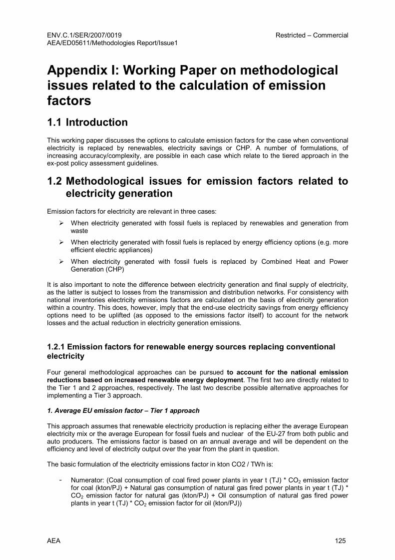
ENV.C.1/SER/2007/0019 Restricted – Commercial AEA/ED05611/Methodologies Report/Issue1
AEA 125
Appendix I: Working Paper on methodological issues related to the calculation of emission factors 1.1 Introduction This working paper discusses the options to calculate emission factors for the case when conventional electricity is replaced by renewables, electricity savings or CHP. A number of formulations, of increasing accuracy/complexity, are possible in each case which relate to the tiered approach in the expost policy assessment guidelines.
1.2 Methodological issues for emission factors related to electricity generation
Emission factors for electricity are relevant in three cases:
Ø When electricity generated with fossil fuels is replaced by renewables and generation from waste
Ø When electricity generated with fossil fuels is replaced by energy efficiency options (e.g. more efficient electric appliances)
Ø When electricity generated with fossil fuels is replaced by Combined Heat and Power Generation (CHP)
It is also important to note the difference between electricity generation and final supply of electricity, as the latter is subject to losses from the transmission and distribution networks. For consistency with national inventories electricity emissions factors are calculated on the basis of electricity generation within a country. This does, however, imply that the enduse electricity savings from energy efficiency options need to be uplifted (as opposed to the emissions factor itself) to account for the network losses and the actual reduction in electricity generation emissions.
1.2.1 Emission factors for renewable energy sources replacing conventional electricity
Four general methodological approaches can be pursued to account for the national emission reductions based on increased renewable energy deployment. The first two are directly related to the Tier 1 and 2 approaches, respectively. The last two describe possible alternative approaches for implementing a Tier 3 approach.
1. Average EU emission factor – Tier 1 approach
This approach assumes that renewable electricity production is replacing either the average European electricity mix or the average European for fossil fuels and nuclear of the EU27 from both public and auto producers. The emissions factor is based on an annual average and will be dependent on the efficiency and level of electricity output over the year from the plant in question.
The basic formulation of the electricity emissions factor in kton CO2 / TWh is:
Numerator: (Coal consumption of coal fired power plants in year t (TJ) * CO2 emission factor for coal (kton/PJ) + Natural gas consumption of natural gas fired power plants in year t (TJ) * CO2 emission factor for natural gas (kton/PJ) + Oil consumption of natural gas fired power plants in year t (TJ) * CO2 emission factor for oil (kton/PJ))

ENV.C.1/SER/2007/0019 Restricted – Commercial AEA/ED05611/Methodologies Report/Issue1
126 AEA
Denominator: (Electricity production with coal fired power plants in year t (TWh)+ Electricity production with natural gas fired power plants in year t (TWh) + Electricity production (TWh) with oil fired power plants in year t + Electricity production (TWh) with nuclear power plants in year t)
A number of points should be noted:
Fuel consumption and electricity generation data are taken from Eurostat CO2 emissions factors for coal, natural gas and oil are based on IPCC default values 32
Both fossil fuels and nuclear generation are assumed to be representative of the average mix of electricity generation options in the EU.
Both public and autoproducers are assumed to be representative of the average mix of electricity generation options.
o However, for autoproducers this assumes that the majority of their electricity production is supplied to the network. Where this is not the case (which may vary across MSs and so be more applicable under the Tier 2 approach – see below) new renewables electricity generation is unlikely to displace electricity generation from autoproducers. In this situation, the fuel consumption and electricity production from such plants can be removed from both the numerator and denominator in the emissions factor calculation
Production of electricity from renewables is not included in the denominator as it is assumed that new renewable electricity is not displacing existing renewable electricity generation.
No adjustment is made to the emissions factor for the coproduction of heat from some public and autoproducer plants. This is because Eurostat only records total fossil fuel consumption rather than an estimate of the split of consumption separately attributable to heat and electricity generation. An adjustment for this could be in theory be made and one possibility is outlined in section 1.2.3.
2. Average national emission factor – Tier 2 approach
This approach is the same as the first one but with the exception that it assumes that renewable electricity production is replacing the MS average domestically applied electricity or fuel mix (for fossils + nuclear) of public and auto producers, as opposed to the EU27 average.
At a MS level the emissions factor for electricity should not account for imports. However, using the calculation under 1) above for fossil consumption and electricity production from plant inside the MS only automatically excludes imports.
3. Emission factors based on marginal power plant in terms of Short Term Marginal Costs (STMC) – Tier 3 approach
The average annual emissions factors calculated under Tier 1 and 2 are a natural simplification. In reality new renewable electricity generation may not displace the grid average. For example, very often a significant share of coal plants is replaced by renewables for the following reasons:
Firstly, during night times gas plants are often not operated but baseload lignite plants dominate the market. Therefore during these times coal plants are replaced in many countries.
Secondly, many gas power plants are coupled with CHP or industrial processes and can not easily turned off. This is a second reason, why coal plants are frequently replaced by renewable generation.
Hence, an average grid emissions factor may understate the true emissions savings if in fact renewables is primarily displacing generation from coal and lignite plant.
One broad option to more accurately assess what kind of generation is being displaced would be to base the determination of the emission factor on marginal power plant in terms of the short term marginal costs (STMC) of the power sector. This approach assumes that the marginal conventional power plant along the merit order curve is replaced regarding to the short term marginal generation
32 See Table 2.2 http://www.ipccnggip.iges.or.jp/public/2006gl/pdf/2_Volume2/V2_2_Ch2_Stationary_Combustion.pdf
ENV.C.1/SER/2007/0019 Restricted – Commercial AEA/ED05611/Methodologies Report/Issue1
AEA 127
costs of the plants. That means that the operation of the power system is optimised in a way that the most expensive fossil and nuclear plants (i.e. the marginal plant) are replaced by renewable electricity. This emission factor depends strongly on the characteristics of the renewable energy sources as well as of the power park as can be calculated with a high time resolution.
The time resolution for the analysis of the short run marginal plant can be calculated with increasing levels of complexity:
a) Assumed marginal plant is the same at all times of the day b) Assumed the marginal plant is seasonal e.g. gas in Summer/coal/lignite in Winter c) Calculated emissions factor based upon a detailed analysis of the merit order – e.g. on an
hourly basis.
Under c) this procedure is far more precise than the one based on average fossil fuel emission coefficients because it is based on the true operation of the power sector, where renewables would replace the marginal power plant in terms of the short term marginal costs (STMC) of the power sector. In this approach the renewable generation replaces the most expensive power plant along the merit order curve in every hour of the year. In this way the plants characterised by high fuel costs (i.e. first oil and gas fired plants, secondly hard coal fired plants, thirdly lignite fired power plants) and low efficiencies are replaced first. It has to be considered however, which part of the power plants is not dispatchable, e.g. due to cogeneration heat. This procedure leads for Germany to an emission coefficient of 0.93 tCO2/ MWh for the years 2004 and 2005 (according to AGESTAT). As compared with approximately 0.62 tCO2 / MWh calculated under the Tier 2 – average national emissions factor approach.
However, for c) such an analysis requires a detailed model based assessment. This is highly sophisticated, since it involves hourly data of electricity demand, renewable electricity generation and power plant operation. Despite the fact that modelling tools showing the required level of detail exist for individual countries (e.g. Germany) a complete assessment of this kind for most EU countries is currently not feasible, although work is underway to extend the model used for Germany also to other countries.
It is, however, possible to approximate the marginal coefficient under approach a) by using the average coefficient across all power plants, which are in principle affected by renewable electricity generation in each country. Generally all thermal power plants except nuclear plants belong in this category. An exception from this general rule is France, where it is assumed that renewable electricity generation affects the operation of nuclear power plants it is assumed that RES generation replaces 70% thermal plants and 30% nuclear plants. Therefore the emission coefficient is calculated based on the assumption that in all countries except France the operation of all thermal power plants is equally affected and the operation of nuclear plants is not affected. As a result of this procedure the emission factors shown in the table below have been determined for the year 2005.
Table 01 Average emission coefficient of the power sector of selected EU countries (including all fossil plants) according to PRIMES
AT CZ DE DK ES FR IT NL PL RO UK EU27 EU15 t/MWh 0.84 1.29 0.96 0.90 0.71 0.70 0.64 0.66 1.22 1.27 0.71 0.86 0.79
As can be seen, the simplified approximation of the STMC emissions factor for Germany (0.96 tCO2 / MWh) is reasonably close to the value calculated under the more sophisticated hourly approach – and is still a better representation of the actual operation of the electricity system than the Tier 2 approach.
This discussion also shows that the generic assumption of a marginal emission factor based only on a gasfired plant, which is supposed to cover the marginal demand, is not supported. This is further detailed for the next method.
4. Emission factors based on marginal power plant in terms of Long Term Marginal Costs (LTMC) – Alternative Tier 3 approach
An alternative approach to the use of STMC to determine what new renewable electricity generation is actually displacing is to assume that the marginal power plant along the merit order curve is replaced
ENV.C.1/SER/2007/0019 Restricted – Commercial AEA/ED05611/Methodologies Report/Issue1
128 AEA
regarding to the long term marginal generation costs of the plants. That means that the investments (covering both fixed costs and assumptions about operating costs) into the power system are optimised in a way that the most expensive fossil and nuclear plants are replaced by renewable electricity – i.e. as opposed to the STMC situation where the optimisation occurs in relation to operating costs only.
This fourth method is mostly relevant in projections and exante evaluations but not in expost evaluations which are at the focus of the methodologies developed here.
1.2.2 Emission factors for energy efficiency measures replacing conventional electricity
The conversion of electricity savings from TWh to Mt CO2 may in principle also be based on the four methods developed for renewables.
However, a key difference is that under Tier 1 and 2 the average EU27 or MS emission factor should cover electricity production from all energy sources (from both public and autoproducers) in the denominator – as the electricity saving when calculated on an average annual basis under these tiers does not discriminate between the source of electricity production.
Under a Tier 3 approach given that the characteristics of efficient appliances and of renewable energy sources are different, it is relevant to discuss to establishment of short term marginal emission factors and their approximation by the average fossil fuel park more in detail.
As discussed for renewables, the most precise procedure under a Tier 3 approach would be the use of an hourly model representation of the power sector in a country together with detailed load profiles for the electric appliances in order to calculate which power plants are substituted by the electricity savings. While such a model exists for example for Germany (the PowerAce model) it does not yet exist for all EU countries although an extension of the PowerAce model is underway. However, there are also limitations in what is known in terms of load patterns of the more efficient appliances.
Therefore in a similar manner to calculating the approximate STMC emissions factor for savings from renewable electricity under Tier 3, a more simplified approach (than the hourly approach) can also be used to calculate the marginal emissions factor for savings from efficiency measures in order to cover all countries.
This can be done by using either the average fossil fuel mix or an existing typical gasfired power plant with a relatively low efficiency 33 of 40% (around 500 g/kWh) depending whether the appliances is mainly or to a large degree used during peaktime (e.g. driers) or has a regular pattern over day and night (e.g. refrigerators). In the absence of precise load patterns for efficient appliances they were classified as follows into two categories.
Table 02 Classification of efficient appliances according to load patterns
Appliances with load patterns mainly or frequently during peak hours
Appliances with load patterns mainly offpeak and during base load time
Washing machine Driers Dishwashers Air conditioners
Refrigerators FridgeFreezers Freezers Lighting
Short term marginal emission coefficient: average gasfired plant
Short term marginal emission coefficient: average fossilfuelfired plant
In addition, to a simplified representation of This approach is simplified in that it uses a rather crude classification, and a number of the appliances cited on the left side will have offpeak users. Similar, part of the righthand devices occurs during peak time or near peaktime. However, there is no statistical information on the usage patterns.
33 This can be justified by the fact that many gasfired plants in the EU are still fairly old and in peak load not used in an optimal range.
ENV.C.1/SER/2007/0019 Restricted – Commercial AEA/ED05611/Methodologies Report/Issue1
AEA 129
1.2.3 Emission factors for CHP replacing conventional electricity
For calculating the CO2 savings from CHP four different directions can be chosen for the reference emission factor for electricity:
1. EU average emission factor – Tier 1 approach 2. National average emission factor – Tier 2 approach 3. Operational margin – Tier 3 approach 4. Built margin – Tier 3 alternative approach
1. EU average emission factor – Tier 1 Approach
The EU average emission factor should be based on the Eurostat data for electricity production for the EU27. A number of choices have to be made:
• base the emission factor on both public supply and auto production, or on public supply only • include renewable energy in the emission factor or not
Furthermore, it is important, since many power plants also produce useful heat, how to deal with the heat production in determining the emission factor. For CHP the following choices are suggested:
• the emission factor should only be based on production from public supply as the majority of auto production is CHP. It does not make sense to compare CHP with itself so only public supply is used.
• Renewables electricity production will hardly/not be affected by increased CHP shares (probably less not true for biomass and hydro power plants that are able to swing opposed to wind and solar) so it is suggested to exclude this.
• As many power plants operate part of the year in CHP mode to supply heat to district heating networks, the CO2 emission factor should be corrected for this. It is proposed to do the correction in the following way: [Useful heat production public supply] / 85% = [Fuel needed for production in heatonly boilers] [Total fuel public supply] [Fuel needed for production in heatonly boilers] = [Fuel needed for electricity production] ([Fuel needed for electricity production] x [weighted average CO2 emission factor fuel mix public supply]) / [total electricity production] = [average CO2 emission factor] 85% is suggested as reference efficiency value for the heat. The correction should be made separately for each fuel category.
2. National average emission factor – Tier 2 approach
For calculating the national average emission factor the same choices are made as for the EU average emission factor. Instead of EU27 data, national data (taken from Eurostat) are to be used. It should be clear whether to include imports and exports of electricity in calculating the emission factor. It is suggested to take the national electricity production and do not include imports in the figures and do not correct for the electricity exported. For countries with very high import shares it might be a good solution to take the weighted national average emission factor of the countries from which the electricity is imported.
3. Operational margin – Tier 3 approach
Instead of using average emission factors it can be decided to use the operational margin approach. In this approach the emission factor is determined by the power plants which need to decrease its power output because of the implementation of CHP plants. Which plant is the operational margin is dependent on several factors:
• The power mix in a country • The dispatch of power plants during the day (peak and off peak) • The dispatch of CHP (baseload or peakonly) • The fuel used in the CHP plant in relation to the fuels used in the other power plants.

ENV.C.1/SER/2007/0019 Restricted – Commercial AEA/ED05611/Methodologies Report/Issue1
130 AEA
On a MS level the operational margin can either be determined based on expert judgement/market knowledge or simulated with sophisticated power models.
4. Built margin – Tier 3 alternative approach
The philosophy of the built margin approach is that the implementation of CHP (and renewables) in the mid and long term (opposed to the short term view of the operational margin approach) leads to a situation where there is no need for a new power plant. This power plant is called the built margin. Which is the built margin on MS level can differ from country to country. In many MS a stateoftheart NGCC (5560% efficiency) is currently considered as the built margin. This can change of course in the course of time (on the longer term a coalfired IGCC with CCS might turn into the built margin).

ENV.C.1/SER/2007/0019 Restricted – Commercial AEA/ED05611/Methodologies Report/Issue1
AEA 131
Annex 1: Structure of the PowerACE model
1. Simulation of electricity markets 2. Detailled datasets
load renewable generation power plants (1200)
3. Calculation of hourly market prices 4. Calculation in computer cluster possible
CO 2 Market
0
10
20
30
40
50
hour
Spotmarket
0
10 20
hour
Services
Industry+ Others
Household
Supplier
Contracts
Transport Renewable Agents
load
bids
GridoperatorTrader
support
load
support
Generator
Supply Trader
meritorder
offer
bid
Primary Reserve Balancing Trader
offer
Gridoperator
bids
Plant DB
plant data
REGLoad DB
REGCapacity DB
Investment Planner
new plant
offer
CO 2 Trader
meritorder
offer
bid
CO 2 Trader Saving Potential Industry DB
Load DB
Demand DB
LoadPrognosis
Investment Planner
new plant
offer
bid
co 2 balance
load profiles
demand+equipment(HH)
Agents
data
Flows
Database
Markets
Demand Renewables
Utilities
Legend Secondary Reserve
Minute Reserve
PumpStorage DB
PumpStorage Trader
offer bid
CO 2 Market
0
10
20
30
40
50
hour
CO 2 Market
0
10
20
30
40
50
hour
Spotmarket
0
10 20
hour
Services
Industry+ Others
Household
Supplier
Contracts
Transport Renewable Agents
load
bids
GridoperatorTrader
support
load
support
Generator
Supply Trader
meritorder
offer
bid
Primary Reserve Balancing Trader
offer
Gridoperator
bids
Plant DB
plant data
REGLoad DB
REGCapacity DB
Investment Planner
new plant
offer
CO 2 Trader
meritorder
offer
bid
CO 2 Trader Saving Potential Industry DB
Load DB
Demand DB
LoadPrognosis
Investment Planner
new plant
offer
bid
co 2 balance
load profiles
demand+equipment(HH)
Agents
data
Flows
Database
Markets
Demand Renewables
Utilities
Legend Secondary Reserve
Minute Reserve
PumpStorage DB
PumpStorage Trader
offer bid
ENV.C.1/SER/2007/0019 Restricted – Commercial AEA/ED05611/Methodologies Report/Issue1
132 AEA
Appendix II: Case Study application of Tier 3 methodology
See separate document “Methodologies Report Appendix II: Case Study application of Tier 3 methodology”

AEA group The Gemini Building Fermi Avenue Harwell International Business Centre Didcot OX11 0QR
Tel: 0870 190 6474 Fax: 0870 190 6318
Tel: 0870 190 6474 Fax: 0870 190 6318