Embed Size (px)
Citation preview
September 1984
EVALUATION OF AUTOMATEDDECISIONMAKING METHODOLOGIESAND DEVELOPMENT OF ANINTEGRATED ROBOTIC SYSTEMSIMULATION
Prepared by:
Dennis C. HaleyBonni J. AlmandMark M. ThomasLinda D. KrauzeKeith D. GrembanJames C. SanbornJoy H. KellyThomas M. Depkovich
This work was performed for NASALangley Research Center underContract NAS1-16759.
The use of specific equipment orcompany brand names in this reportdoes not in any way constitute endorsementof those products or companies.
MARTIN MARIETTA AEROSPACEDENVER AEROSPACEP.O. Box 179Denver, Colorado 80201
https://ntrs.nasa.gov/search.jsp?R=19850005207 2018-06-08T10:09:30+00:00Z
CONTENTS
INTRODUCTION 1Background 1Contract Objectives 3Report Organization 3
MANIPULATOR SYSTEM DEFINITION 6Arm Creation/Modification 7
Base 8Joint/Link 8End Effectors 11Graphics 12
Environment Creation/Modification 12Load Objects Creation/Modification 14System Creation 15
ANALYSIS CAPABILITY 18Introduction 18Kinematic Analysis . . 21
Link Positioning 21Link and Point Velocities 24Link and Point Accelerations 25End Effector Motion 26Task-Oriented Motion Specification 29
Requirements Analysis 33Joint Reaction Forces and Torques 33Actuator Drive Torques 34Presentation of Results 35
Response Simulation 35Actuator Driving Torques . 36Position- and Velocity-Related Torques 37Effective Inertia Matrix 38Joint Friction 39Motion Constraints 40Impact of Collision 44Coulomb Friction at the Constraint Points . . . . . . 45
Modeling the ISRL Multisensor End Effector 47Configuration of the ISRL End Effector 47Geometry of Gripper Operation 50Gripper Dynamics 52Grasping a Load Object 55End-Effector Force Sensing 57
POSTPROCESSING CAPABILITY 59Introduction . . . . . 59Simulation Replay .. 59Simulation vs Hardware Replay 60Parameter Plots 60
11
MANIPULATOR CONTROL 63Manipulator Description 63
Kinematics 64Manipulator Dynamics 65Performance Requirements 65
Control Algorithms 68Linear Discrete Control 68Resolved Acceleration Control 75Resolved Motion Force Control 75
Adaptive Control 84Parameter Estimation 84Linear Adaptive Control 86Nonlinear Adaptive Control 90Parameter Estimation ... 91Model-Matching Control 96
Force/Torque Control 102Hybrid Control 105Active Stiffness Control 108
MANIPULATOR TRAJECTORY PLANNING 112History and Development of Path Planning Methods 114
Graph Search of Discretized Environments 114Visibility Lines and Growing Obstacles 115Graph Search of Representations of Free Space 116
Path Planning Research Under the ROBSIM Contract 117The Generalized Cone Method 117The Joint Space Method , 117The Incremental Constrained Motion Method 121
Comparison of Current Methods and Directions forFurther Study 126
The Generalized Cone Representation of Free Space . . . 126Modeling Physical Environments in Joint Space . . . . . 127The Incremental, Constrained Motion Method 127Directions for Further Study 127
IMAGE PROCESSING AND VIDEO SIMULATION 129Edge Detection 129
Detecting Edge Pixels 129Thinning Edge Pixels 131Linking Edge Pixels 133
SIMULATION VALIDATION 137Planar Arm Parameter Identification 137Simulation Comparison - Elbow 139Simulation Comparison - Shoulder 142Simulation Comparison - Combined Motion 143PUMA Parameter Identification 147
CONCLUDING REMARKS . . . . 156REFERENCES 160
111
Figure Page
1 ROBSIM Functional Blocks 42 Hinge, Swivel and Sliding Joints 93 Joint/Link Sequencing 104 Detailed Graphics Representation of Manipulator Arm ... 135 Load Local and Component Coordinate Systems . . . . . . 156 Complete System Definition 177 Kinematic Representation of Serial Manipulator 218 Constant-Acceleration Constant-Velocity Constant-
deceleration Profile 319 Results of Simulation Driven by Torques, Generated in
Requirements Analysis 3610 Coulomb/Static Friction on System Response 4011 Effect of Static Friction at Joint 4112 Constrained Motion of End Effector 4213 ISRL End Effector 4814 Functional Components of the ISRL Gripper . . . . . . . 4915 Kinematics of the ISRL Gripper 5116 Block Diagram Representing the Dynamics of Gripper
Operation 5317 Location of Cylindrical Peg 5618 Critical Contact Points Between Peg and Jaw Surface ... 5619 Jaw Forces Resulting from an Applied Load and Gripping
Force 5820 Simulation vs Hardware Replay 6121 Joint Displacements 6222 Six-Degree-of-Freedom Manipulator 6423 Manipulator Joint Position Solution Procedure 6424a Three-Link Planar Arm 6624b Three-Link Planar Arm Dynamic Equations 6725 Two-Link Planar Manipulator Definitions 6826 General Controller Structure 6927 Pole-zero Compensator 7028 PID Controller 7129 System Pole-Zero Diagram 7230 Root Locus with Pole Cancellation 7331 General Control Loop with Disturbances, W(Z) 7432 General Adaptive Controller 8433 General Parameter Estimation 8534 Model Reference Control Structure , 8835 Linear Adaptive Control Simulation 8936a Three-DOF Adaptive Control Simulation Results - Joint 1 9936b Three-DOF Adaptive Control Simulation Results - Joint 2 . . 10036c Three-DOF Adaptive Control Simulation Results - Joint 3 . . 10137 Compliant Control for Peg Insertion 10238 Rigid Peg Supported Compliantly by Lateral Spring Ky
and Angular Spring KI at Distance Lg from Peg's Tip . . . 10339 Scheinman Force-Sensing Wrist . 10440 Conceptual Organization of Hybrid Controller 105
IV
41 Hybrid Controller Implementation 10642 Hybrid Control Simulation Configuration 10743 Profile of Controlled Force Component . . 10744 Stiffness Control System 10945 Stiffness Control System Implementation in ROBSIM . . . . 11046 Active Compliance Control Ill47 Discretization of the Environment 11448 Visibility Line Method of Path Planning 11549 Path Planning in Complex Environment 11650 Joint Space Method of Path Planning 11851 Visibility Line Method in Three Dimensions . . . . . . 11952 Translation Functions from Physical to Angle Space . . . . 12053 An Hierarchical Object Representation 12054 Path Planning in Joint Space 12155 Arm Position in Cluttered Environment 12256 Constrained Motion of Joint 12357 Actions of a Rule-Based Planner 12558 Classification of Edge Types (after Shirai [1978]) . . . . 13459 PUMA Manipulator 13560 Planar Arm Configuration 13761 Elbow Simulation and Hardware Positions, Sinusodal Motion . 14162 Elbow Simulation and Hardware Positions, Trapezoidal Motion . 14163 Shoulder Simulation and Hardware Positions 14264 Hardware and Simulation Shoulder Position for Combined
Motion 14465 Hardware and Simulation Elbow Positions for Combined Motion . 14466 Shoulder Hardware and Simulation Positions after Offset , - 14567 Shoulder Hardware and Simulation Positions, Combined Motion . 14668 Elbow Hardware and Simulation Positions, Combined Motion . . 14669 Kinematic Parameters of the PUMA 14770 Locating a Point on the Joint Axis 14871 PUMA Mass/Centroid Parameters 15072 Static Load Measurement Configuration 15173 PUMA Joint 3 Position Profile 15474 PUMA Joint 3 Velocity Profile 15475 PUMA Joint 3 Acceleration Profile 15576 Preliminary ROSS Simulation Graphics Display 15777 Display of robot Arm Converted from a CAD/CAM DataBase . . 158
Table
I System Definition Symbols 7II Notation in Analysis Capabilities Discussion . . . . . . 19III Nonlinear Approximations . 69IV Notation for Manipulator Path-Planning Section 113V Planar Arm Link Mass Properties 138VI Motor Parameters Initially Used in Simulation 139VII Planar Arm Motor Parameters 143VIII PUMA Kinematics 148IX Comparison of PUMA Characteristics 148X Measured Friction and Gravity Forces . . . . . . . . 150XI Joint Static Friction Torques 152
SUMMARY
Work tasks that require extensive manual labor in hazardous environments,(e.g., NASA advanced missions) would derive great benefit from increased use ofautomation technology. This report documents a NASA-sponsored activity to de-velop the specific technologies needed for increasing the role of automation insuch missions and to implement a generic computer simulation capability formanipulator systems.
The computer simulation developed provides the ability to perform kinema-tic and dynamic analysis of user-defined manipulators. The user establishes amanipulator system model, including arms, load objects and an environment, inresponse to program prompts. The task profile is also specified interactivelyby the user and consists of motion segments utilizing position or rate controlin joint or end-effector motion coordinates, and such nonmotion steps as GRASP(for grasping a load object).
The kinematic analysis provides positions, velocities, and accelerationsof all parts of the system for the prescribed motion; it incorporates a robustiterative joinc solution algorithm for generality. The dynamic analysisprocedures include requirements analysis, which calculates the system loadsfor specific motions, and response simulation, which gives the motiontrajectory resulting from a prescribed set of driving torques or feedbackcontrol law.
The analysis results can be displayed as printed tabular output or plotsof the trajectories of relevant parameters. Animated graphic display is avail-able during system creation and analysis to verify the system configuration andmotion.
The specific automation technologies investigated include control systemdesign, trajectory planning and image processing. A general overview of con-trol system design is presented, with special emphasis on adaptive control andhybrid control of forces and positions. Computer simulation of these controlmodes is available.
Three algorithms for generating collis ion-free paths through cluttered en-vironments were implemented and compared. The algorithms include a joint spacesearch method, a method in which free space is represented by a collection ofgeneralized cones, and an incremental motion procedure in which constraints aretranslated locally into joint coordinates. The benefits and drawbacks of eachmethod are discussed.
The literature on edge detection is reviewed in this report. An edge-detection algorithm was implemented, along with a computer simulation of amanipulator—mounted camera for vision sensing.
Appendices to this report describe in detail the programming and use ofthe computer simulation package (available through COSMIC).
vi
INTRODUCTION
Background
This document reports the results of work performed in Tasks 9 through 20of contract NAS1-16759, Evaluation of Automated Decisionmaking Methodologiesand Development of an Integrated Robotic System Simulation. It was preparedby Martin Marietta Denver Aerospace for the Langley Research Center of theNational Aeronautics and Space Administration (NASA-LRC) in accordance with thecontract statement of work. These tasks constitute Phases II and III of a mul-tiphase activity addressing the technologies relevant to design and operationof advanced manipulator systems. Phase I of this activity concentrated on theidentification and evaluation of artificial intelligence techniques applicableto NASA advanced missions and on developing a framework and mathematical modelsfor the computer simulation of manipulator systems. The results were docu-mented in 1982 (NASA Contractor Reports 165975, 165976 and 165977).
This project is motivated by the realization that NASA advanced missionsrequire increasing use of automation technology for both economical and per-formance reasons. Factors influencing this trend include:
1) . The cost of supporting man in the hostile space environment is muchgreater than that of supporting an unmanned system;
2) Human strength, dexterity, reach and precision are too limited forsome applications;
3) A well-designed automated system provides more optimal control than ahuman controller;
4) Many mission tasks are highly repetitive and mundane. Automationtechnology is ideally suited for such applications, while humans tendto become bored and make more mistakes;
5) Automation systems are better suited for round-the-clock operationsthat more fully utilize limited resources on space missions.
Despite these drawbacks involved in direct human operation or control,the adaptability, resourcefulness and problem-solving ability of man are stillneeded for the complex dynamic environment associated with space applications.Current robot systems are limited to relatively simple, preprogrammed tasks instructured environments and incorporate very little machine intelligence andexternal sensing. To achieve the ambitious goals of the space program in suchareas as space station and long-life reserviceable spacecraft, it is essentialto reduce direct human control of the robotic systems. This reduction can mostnaturally occur over a four-phase development process.
The first phase is to develop the required system with man in the loop toprovide control and the problem-solving functions. The second phase of roboticsystem evolution is to extract the man from the primary control loop to assumea supervisory role. In this role, the operator will perform the function ofplanning out a sequence of tasks to achieve a specific goal. The robotic sys-tem will perform the tasks of trajectory planning, obstacle avoidance, andjoint control. In the third phase, the individual will be extracted one morelevel. In this phase, the operator will perform the function of establishingintermediate goals for the robotic system. The robotic system will perform thefunctions associated with breaking down the specific goals into individualtasks to be performed. The final phase of robotic system development will re-sult in a fully autonomous robotic system.
To accomplish these goals requires dramatic improvement in some of the ma-nipulator component technologies, especially in the fields of sensing, controland artificial intelligence. This contract activity addressed several of theseissues; implementations were developed for image processing (edge detection),intelligent path planning, and advanced control strategies (including adaptivecontrol and hybrid force/position control).
Development of the complex technologies associated with advanced automa-tion in a timely and cost-efficient manner requires extensive use of computersimulation tools that allow implementations to be evaluated and compared be-fore building hardware prototypes. The capabilities that a kinematic simula-tion (i.e., one in which motions, not forces, are considered) can provide in-clude:
1) Find and display manipulator dexterity and workspace. This can beused to evaluate kinematic designs, suggest workcell arrangement(where feasible), and help design systems for maintenance and repairby automation;
2) Verify and implement path planning, including obstacle avoidance andsingularity detection;
3) Evaluate improvement in system operation from some types of sensorssuch as proximity sensors or moving video cameras;
4) Determine potential speed of operation;
5) Training for teleoperator control using the simulation instead ofhardware, and evaluate the different levels of human interaction inthe control loop.
A dynamic simulation also includes the system forces and provides addi-tional capabilities such as:
1) Verification and evaluation of controller designs, especially thosethat incorporate advanced control concepts. For example, adaptivecontrol schemes often involve identification of system parameters fromresponse information. With a dynamic simulation, the actual valuesfor the parameters are specified so the identification scheme canreadily be verified;
2) Verification of system performance, structural integrity, load distri-bution and component stress levels;
3) Testing the use of force—related sensors such as a force/torque wristor gripper force sensors in system operation;
4) More accurate simulation for teleoperator training, including controlinvolving force-feedback or dynamic interactions with the environment.
A dynamic simulation package for the entire manipulator system forms an indis-pensable tool for design and development of automation implementations for NASAadvanced missions.
Contract Objectives
The primary objectives of this contract activity are the implementationof an integrated robotic simulation package and development of the technolo-gies relevant to operation of advanced manipulator systems. The research per-formed and software developed during the contract phases reported here focusedon the following capabilities:
1) Computer simulation of a robot in operation, including system kine-matics anvi uynaiu3.cs, interactive contro.*. GJ. program execution **y <_n&user, and graphic display of the system operation;
2) Computer simulation of multisensor grippers;
3) Control concepts for manipulators incorporating adaptive techniquesand control of force levels as well as positions;
4) Trajectory planning for manipulator motions in unstructured environ-ments ;
5) Image processing and simulation of a manipulator-mounted video camera.
Report Organization
This report consists of a main text that describes the study results, in-cluding the technical aspects of the robotic simulation (ROBSIM) package and ofthe automation technologies investigated, along with two appendices that docu-ment the computer implementation of ROBSIM. ROBSIM consists of three func-tional packages (Fig. 1):
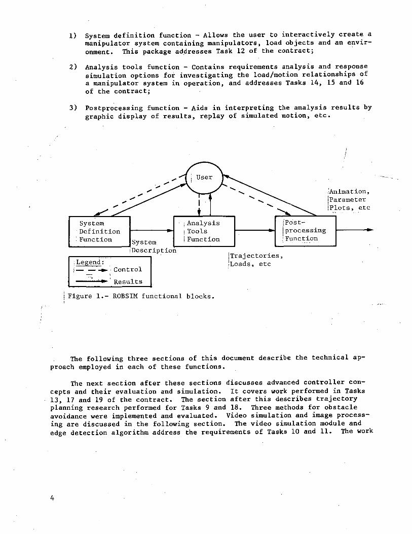
1) System definition function - Allows the user to interactively create amanipulator system containing manipulators, load objects and an envir-onment. This package addresses Task 12 of the contract;
2) Analysis tools function - Contains requirements analysis and responsesimulation options for investigating the load/motion relationships ofa manipulator system in operation, and addresses Tasks 14, 15 and 16of the contract;
3) Postprocessing function - Aids in interpreting the analysis results bygraphic display of results, replay of simulated motion, etc.
('Animation,ParameterPlots, etc
SystemDefinitionFunction System
(Description
iAnalysisiToolsI Function
Post-processingFunction
iLegend:i— — -»-. Control
Results
(Trajectories,JLoads, etc
Figure 1.- ROBSIM functional blocks.
The following three sections of this document describe the technical ap-proach employed in each of these functions.
The next section after these sections discusses advanced controller con-cepts and their evaluation and simulation. It covers work performed in Tasks13, 17 and 19 of the contract. The section after this describes trajectoryplanning research performed for Tasks 9 and 18. Three methods for obstacleavoidance were implemented and evaluated. Video simulation and image process-ing are discussed in the following section. The video simulation module andedge detection algorithm address the requirements of Tasks 10 and 11. The work
in Task 20, hardware vs software validation, forms the next section. This sec-tion was addredded with cooperation from NASA-LRC. Validation efforts werecarried out on a 2 DOF planar arm at Martin Marietta and a 6 axis PUMA robot atNASA-LRC. The final section of this text summarizes the results of this activ-ity and describes avenues for further efforts to expand, enhance and utilizecapabilities developed during the performance of this contract.
This document has two appendices available through COSMIC.* Appendix Ais a ROBSIM User's Guide and describes the steps involved in running the pro-gram. Appendix B provides the programmer with additional information concern-ing program implementation. This appendix and the in-code documentation pro-vide sufficient information to allow modification of the program for special-purpose applications.
* Inquiries concerning the program ROBSIM, Appendix A (User's Guide), andAppendix B (Programmer's Guide) should be directed to: COSMIC, 112 BarrowHall, University of Georgia, Athens, GA 30601.
MANIPULATOR SYSTEM DEFINITION
This section describes the methods implemented in the ROBSIM package fordefining a robotic manipulator system. The discussion of the system definitionis separated into four subsections:
1) Manipulator arm creation/modification;
2) Environment creation/modification;
3) Load objects creation/modification;
4) System creation.
A system is actually composed of one or more of the components listed in items1) through 3) above.
Manipulator arm creation/modification is used to define the mass and geo-metric properties of one robot arm. This includes properties for the base, alljoint/link pairs, and the end-effector (also called "tool" or "hand"). De-tailed geometries may also be defined for each part of the arm. These, how-ever, are used for the graphics displays that accompany the ROBSIM frameworkand do not affect arm motions or any of the analyses methods described later.
Environment creation/modification is used to simulate immovable objects inthe workspace of the manipulator arm. Currently the usefulness of the environ-ment definition is limited to graphic displays and does not affect or hinderthe manipulator motion in any way.
Creation/modification of load objects is very similar to that of the en-vironment, with the exception that load objects may be moved around the work-space by one or more manipulator arms.
System creation is used to bring together the components into one coherentgroup. A system may contain as little as one manipulator arm or multiple arms,a detailed environment, and a group of load objects. Each component is placedin the system with respect to a reference or world coordinate system. Table 1lists the notations used in this section.
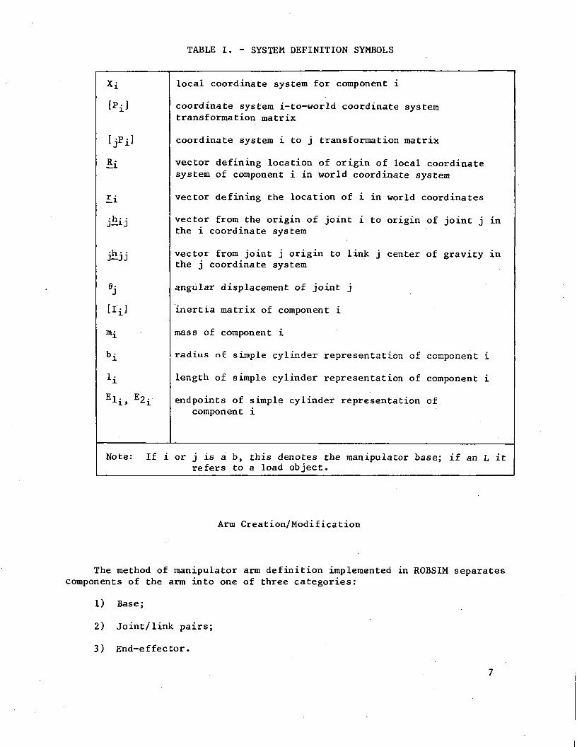
TABLE I. - SYSTEM DEFINITION SYMBOLS
Xi
[Pi]
[jpi]Ri
Iijhij
jhjj
BiHi]mi
bi
li
Ei . Eo .Ai> ^i
local coordinate system for component i
coordinate system i-to-world coordinate systemtransformation matrix
coordinate system i to j transformation matrix
vector defining location of origin of local coordinatesystem of component i in world coordinate system
vector defining the location of i in world coordinates
vector from the origin of joint i to origin of joint j inthe i coordinate system
vector from joint j origin to link j center of gravity inthe j coordinate system
angular displacement of joint j
inertia matrix of component i
mass of component i
radius of simple cylinder representation of component i
length of simple cylinder representation of component i
endpoints of simple cylinder representation ofcomponent i
Note: If i or j is a b, this denotes the manipulator base; if an L itrefers to a load object.
Arm Creation/Modification
The method of manipulator arm definition implemented in ROBSIM separatescomponents of the arm into one of three categories:
1) Base;
2) Joint/link pairs;
3) End-effector.
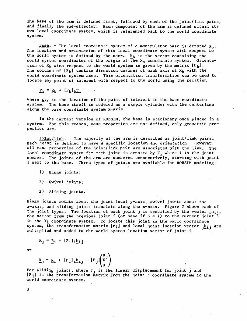
The base of the arm is defined first, followed by each of the joint/ link pairs,and finally the end-effector. Each component of the arm is defined within itsown local coordinate system, which is referenced back to the world coordinatesystem.
Base. - The local coordinate system of a manipulator base is denoted Xfc.The location and orientation of this local coordinate system with respect tothe world system is defined by the user. Rj, is the vector containing theworld system coordinates of the origin of the X^ coordinate system. Orienta-tion of Xfo with respect to the world system is given by the matrix [P l •The columns of [P ] contain direction cosines of each axis of Xjj with theworld coordinate system axes. This orientation transformation can be used tolocate any point of interest with respect to the world using the relation
££ = R,, + [Pblbli
where .£1 is the location of the point of interest in the base coordinatesystem. The base itself is modeled as a simple cylinder with the centerlinealong the base coordinate system x-axis.
In the current version of ROBSIM, the base is stationary once placed in asystem. For this reason, mass properties are not defined, only geometric pro-perties are.
Joint/link. - The majority of the arm is described as joint/ link pairs.Each joint' is defined to have a specific location and orientation. However,all mass properties of the joint/ link pair are associated with the link. Thelocal coordinate system for each joint is denoted by X^ where L is the jointnumber. The joints of the arm are numbered consecutively, starting with joint1 next to the base. Three types of joints are available for ROBSIM modeling:
1) Hinge joints;
2) Swivel joints;
3) Sliding joints.
Hinge joints rotate about the joint local y-axis, swivel joints about thex-axis, and sliding joints translate along the x-axis. Figure 2 shows each ofthe joint types. The location of each joint j is specified by the vector i£i j >the vector from the previous joint i (or base if j = 1) to the current joint jin the X^ coordinate system. To locate this joint in the world coordinatesystem, the transformation matrix [P ] and local joint location vector ihj^multiplied and added to the world system location vector of joint i
Rj = R£ + [Pi
or
Rj =
for sliding joints, where 0j is the linear displacement for joint j and[Pj] is the transformation matrix from the joint j coordinate system to theworld coordinate system.
8
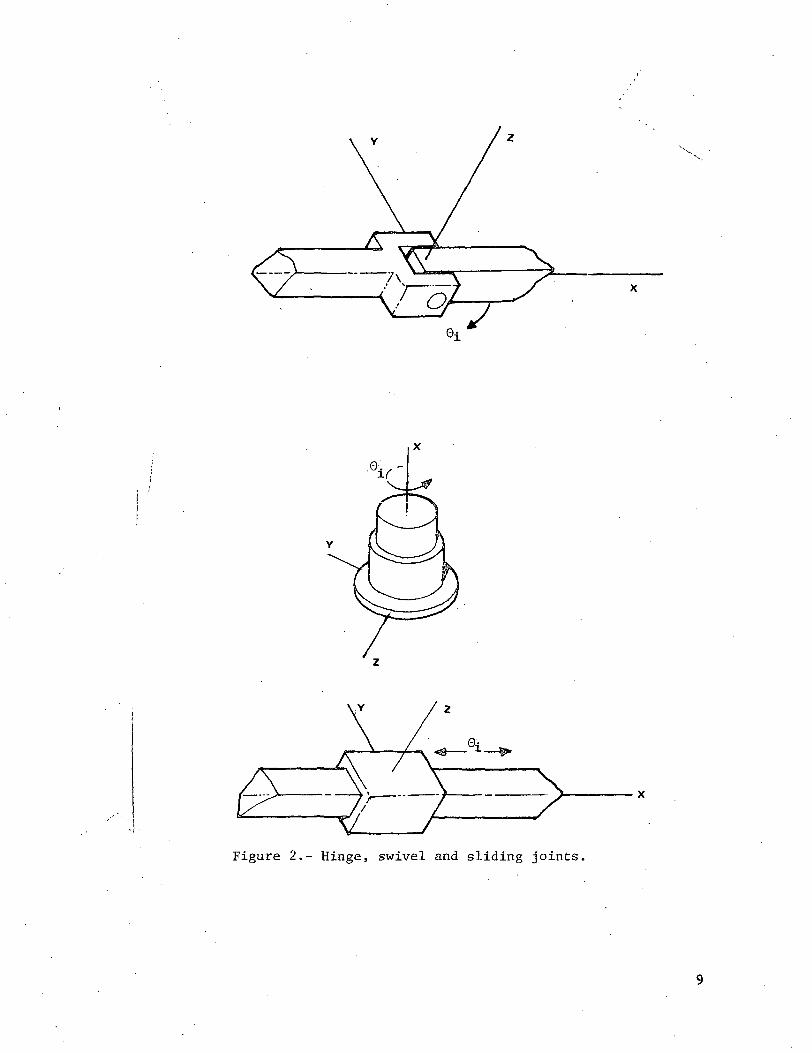
/\
v /Figure 2.- Hinge, swivel and sliding joints.
Joint orientation is also defined with respect to the previous joint withthe transformation matrix liPjl. Each column contains the direction co-sines of an axis of the Xj coordinate system to the X^ coordinate systemaxes. The transformation matrix [Pj] is then calculated from
The capability for user-defined effective actuator parameters is included foreach joint. These parameters are:
1) Actuator torque constant;
2) Motor gear ratio;
3) Actuator amplifier gain;
4) Back EMF constant;
5) Motor effective inertia;
6) Motor winding resistance;
7) Motor winding inductance;
8) Coulomb friction coefficient;
9) Static friction coefficient;
10) Effective viscous damping.
The use of these parameters is discussed in detail in the Analysis Capabilitysection. The initial joint position '? j is the displacement of the jointmeasured from its original location and orientation.
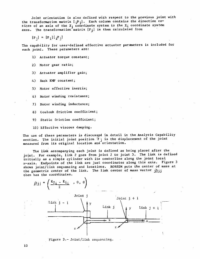
The link accompanying each joint is defined as being placed after thejoint. For example, link 2 goes from joint 2 to joint 3. The link is definedinitially as a simple cylinder with its centerline along the joint localx-axis. Endpoints of the link are just coordinates along this axis. Figure 3shows joint/ link sequencing and locations. ROBSIM puts the center of mass atthe geometric center of the link. The link center of mass vector jhjjthen has the coordinates.
0, Oj
Link j - 1
Figure 3.- Joint/link sequencing.
10
Multiplying by [Pj] transforms this vector to the world coordinate system.As an alternative to this placement of the center of mass, an arbitrary centerof mass may be defined by user input of the local system coordinates of the de-sired center of mass. The algorithm implemented in ROBSIM for calculating thelink inertia matrix uses the following equations for computing the diagonalterms
i-3 3 = *2 2
The off-diagonal terms are set to zero as there are no cross-products of in-ertia for the simple cylinder representation used to model the links. To spe-cify a different inertia matrix, the user may input values directly.
Point masses may be added to each link if desired to create an arbitrarymass distribution. The addition of point masses requires that the total mass,center of gravity, and inertia matrix of the link be recalculated. The totalmass is simply the sum of the link mass and all associated point masses
# of ptsmitotal = mi +2_)mn
n=l
The new center of gravity is determined using
\-> r
Calculating a new inertia matrix is done using
t1^ total = t1^ + "il1^
where [E] is the identity matrix and _bj is the vector from the newcomposite eg to the eg of j (link or point mass).
It should be noted that in addition to the three joint types mentioned earlier,"special joints" where the motion between adjacent joints may be constrainedare also provided for. However, the use of any special joint would require aprogram modification that is not readily available at this time.
End-effectors . - The end-effector of a manipulator arm is modeled exactlyas the link of a joint/ link pair and includes the same provisions as links dofor specifying arbitrary mass distributions.
11
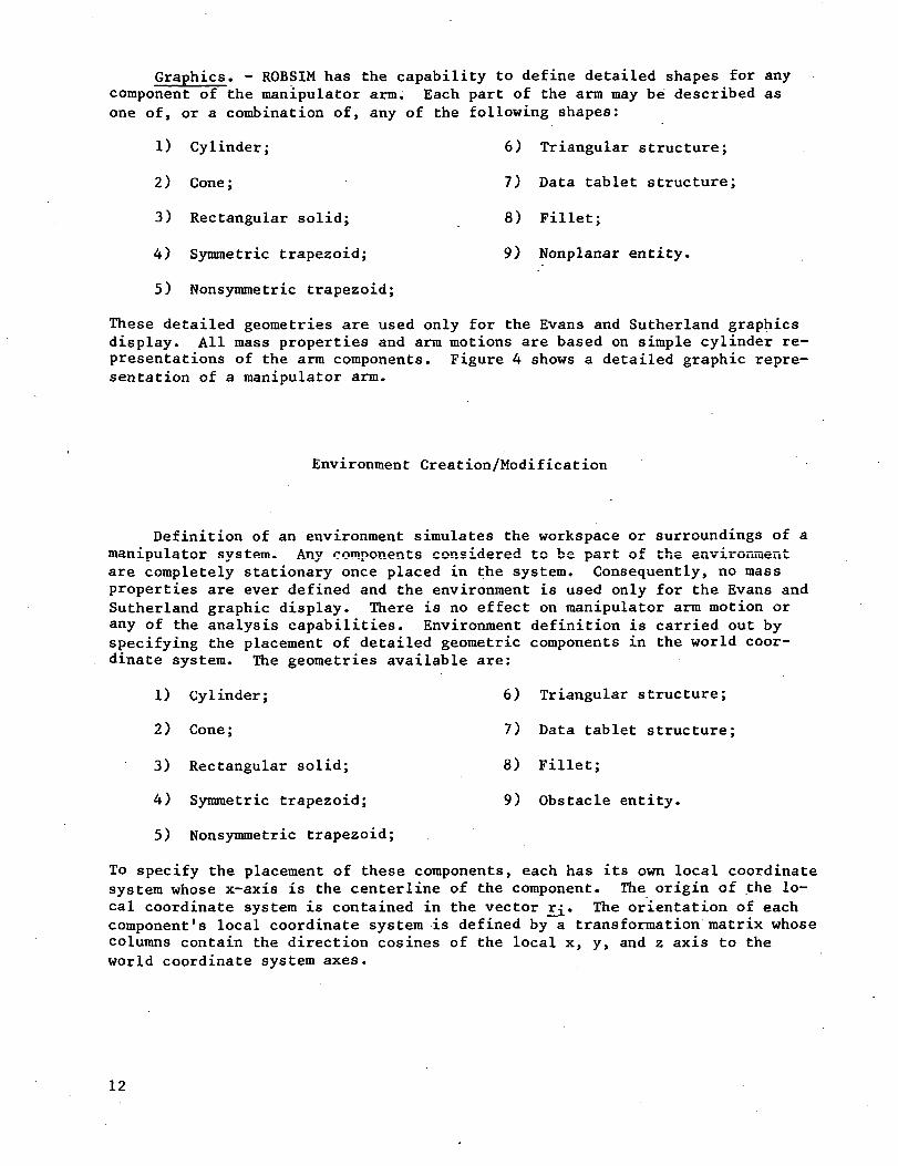
Graphics. - ROBSIM has the capability to define detailed shapes for anycomponent of the manipulator arm. Each part of the arm may be described asone of, or a combination of, any of the following shapes:
1) Cylinder;
2) Cone;
3) Rectangular solid;
4) Symmetric trapezoid;
5) Nonsymmetric trapezoid;
6) Triangular structure;
7) Data tablet structure;
8) Fillet;
9) Nonplanar entity.
These detailed geometries are used only for the Evans and Sutherland graphicsdisplay. All mass properties and arm motions are based on simple cylinder re-presentations of the arm components. Figure 4 shows a detailed graphic repre-sentation of a manipulator arm.
Environment Creation/Modification
Definition of an environment simulates the workspace or surroundings of amanipulator system. Any components considered to be part of the environmentare completely stationary once placed in the system. Consequently, no massproperties are ever defined and the environment is used only for the Evans andSutherland graphic display. There is no effect on manipulator arm motion orany of the analysis capabilities. Environment definition is carried out byspecifying the placement of detailed geometric components in the world coor-dinate system. The geometries available are:
1) Cylinder;
2) Cone;
3) Rectangular solid;
4) Symmetric trapezoid;
5) Nonsymmetric trapezoid;
6) Triangular structure;
7) Data tablet structure;
8) Fillet;
9) Obstacle entity.
To specify the placement of these components, each has its own local coordinatesystem whose x-axis is the centerline of the component. The origin of the lo-cal coordinate system is contained in the vector r_£. The orientation of eachcomponent's local coordinate system is defined by a transformation matrix whosecolumns contain the direction cosines of the local x, y, and z axis to theworld coordinate system axes.
12
ROBOTIC SYSTEM SIMULRTICN PROGRRM CROBSIM)
SYSTEM DEFINITION - DETOI1.ED GEOMETRY REPRESENTRTION
MARTIN MARIETTA
Figure 4. - Detailed graphics representation of manipulator arm.
13
Load Objects Creation/Modification
Load objects are similar to the environment in that they are used to sim-ulate the workspace of a manipulator. Unlike components of the environment,load objects are not stationary but may be moved by a manipulator arm. Similarto arm link components, each load object is defined initially as a simple cyl-inder with a local coordinate system XL, and with the centerline of the ob-ject along the local x-axis. The location of the origin of the X£ coordinatesystem is defined by the vector rT. The orientation of the local coordinatesystem is again defined by a transformation matrix whose columns are the direc-tion cosines of the local x, y and z axes to the world coordinate system axes.
The center of mass of each load object is determined using the method de-scribed for manipulator links. A different center of mass may be specified byuser definition of its x, y, and z coordinates in the XL coordinate system.Inertia matrix calculations are also the same as for the links of a manipulatorarm. Point masses may be added to a load object to create an arbitrary massdistribution. The location of the point mass is defined by the vectorT.rrt-. The new mass properties (total mass, center of gravity, and inertiamatrix) are calculated by the same algorithms as used for the manipulatorlinks.
The preceding paragraphs have described the mass properties for load ob-jects. Evans and Sutherland graphic displays are available to portray the loadobjects. This capability allows the description of detailed geometries foreach object. The detailed geometry definition is done by describing each loadobject as a group of one or more of the following geometry components:
1) Cylinder; 6) Triangular structure;
2) Cone; 7) Data tablet structure;
3) Rectangular solid; 8) Fillet;
4) Symmetric trapezoid; 9) Nonplanar entity.
5) Nonsymmetric trapezoid;
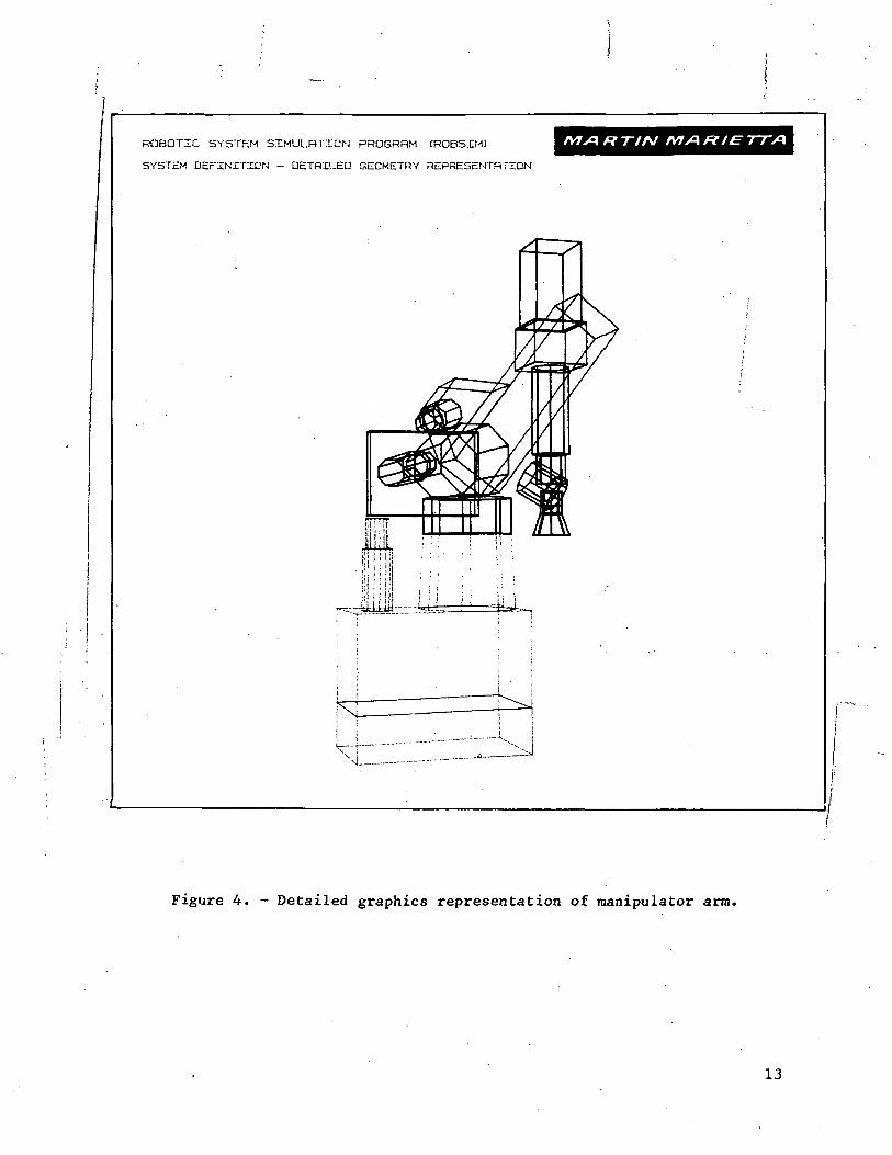
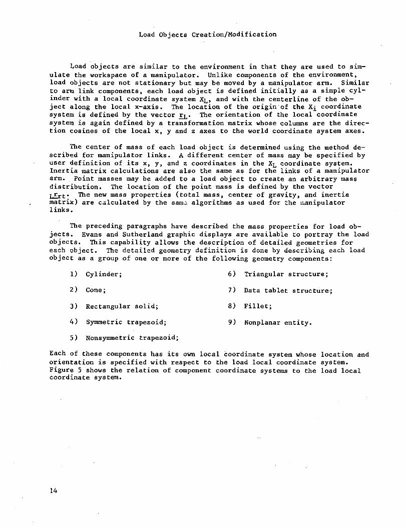
Each of these components has its own local coordinate system whose location andorientation is specified with respect to the load local coordinate system.Figure 5 shows the relation of component coordinate systems to the load localcoordinate system.
14
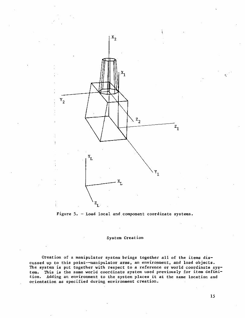
ZL
Figure 5. - Load local and component coordinate systems,
System Creation
Creation of a manipulator system brings together all of the items dis-cussed up to this point—manipulator arms, an environment, and load objects.The system is put together with respect to a reference or world coordinate sys-tem. This is the same world coordinate system used previously for item defini-tion. Adding an environment to the system places it at the same location andorientation as specified during environment creation.
15
Placement of a manipulator arm in the system may be modified from the lo-cation and orientation called out during arm creation. The new location of thearm base is stored in the same vector R|j. Location vectors for each jointare also updated. The new base orientation is a concatenation of the matrix[P!J] specified during arm creation and the matrix [bPfo'l* which specifiesthe new orientation with respect to the old orientation. The transformationmatrix for the new base orientation with respect to the world is found using
The orientation of each joint in the rest of the manipulator arm is revisedusing the same procedure
[PI-] = [PiHbPb']Placement of load objects in the system is identical to manipulator arm
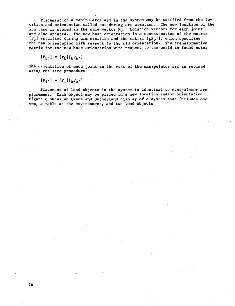
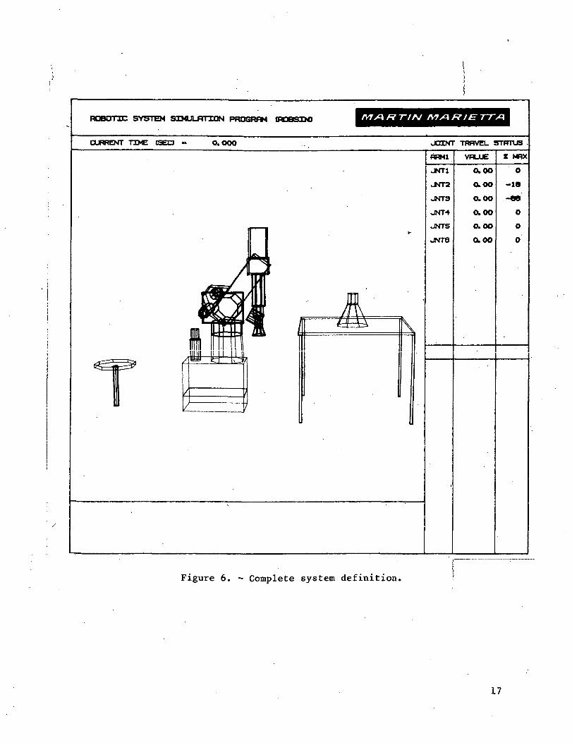
placement. Each object may be placed in a new location and/or orientation.Figure 6 shows an Evans and Sutherland display of a system that includes onearm, a table as the environment, and two load objects
16
MJUUI1C SYSTEM SXMJLJPrrXON PRttgWM (ROBSXM) AT>q Ff TIN A7X1 FT/E 7TX1
CURRENT TIME (SEO « O. OOO JOINT TRRVEL STPTTUS
flRMl
JNT1
JNT2
JNT3
JNT4
JNTS
JNT6
VPLUE
Ok 00
O.OO
0.00
0.00
0.00
0,00
X MRX
O
-IS
O
O
0
Figure 6. - Complete system definition.
17
ANALYSIS CAPABILITY
Introduction
This section describes the analysis tools implemented in the ROBSIM pack-age for investigating load and motion properties of general manipulator sys-tems. Three types of analysis can be performed on the user-defined system:
1) Kinematic analysis;
2) Requirements analysis;
3) Response simulation.
Kinematic analysis involves determining positions and position derivatives(motion) of the manipulator links. It is important in its own right for in-vestigating arm reachability, workpiece placement, task sequencing, obstacleavoidance, tool rate limits, etc; it also forms the basic step in all appropri-ate dynamic analysis formulations.
Requirements analysis and response simulation are the two dynamic analysisoptions available in the ROBSIM package. Requirements analysis, also referredto as "inverse dynamics" or "kinematically driven analysis," involves determi-ning the operating forces and torques for a prescribed motion state of the ma-nipulator. This provides actuator torque and sizing criteria, component stress.levels, load-handling limits, feedforward compensation values for control, etc.
For response simulation, or "force-driven analysis," the actuator drivingtorques are specified (possibly in the form of a feedback control law) and theresulting motion trajectory of the manipulator is calculated. This option isespecially useful for evaluating control strategies, task performance, inter-actions with the environment, etc.
The final part of this section describes the algorithms employed in theROBSIM package for modeling end-effectors, in particular the parallel jawgripper developed and in use at the Intelligent Systems Research Laboratory(ISRL) at NASA-LRC.
Some results obtained using these ROBSIM analysis tools are demonstratedin subsequent sections of this report. Table II lists the notation used inthis section.
18
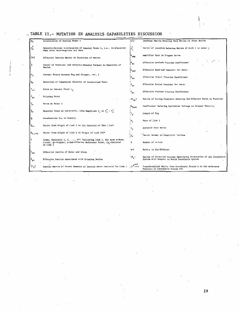
„ TABLE II.- NOTATION IN ANALYSIS CAPABILITIES DISCUSSION
Acceleration of Special Point i
Velocity-Related Acceleration of Special Point i, i.e., AccelerationWhen Joint Accelerations Are Zero
Effective Inertia Matrix in Equations of Motion
Vector of Position- and Velocity-Related Torques in Equations ofMotion
Contact Points between Peg and Gripper, i«l, 2
Direction of Tangential Velocity of Constrained Point
Force at Contact Point c.
Gripping Force
Force at Point i
Reaction Force,at
Acceleration D^e to Gravity
Vector from Origin of Link i to the Centroid of That Link*
Vector from Origin of Link 1 to Origin of Link 1+1*
Index, Generally 1, 2, ..., N+l Indicating Link i, But Also b-Base,L-Load, gr-Gripper, p-End-Effector Reference Point, eg -Centroidof Link i
Effective Inertia of Motor and Drive
Effective Inertia Associated with Gripping Motion
Inertia M&trix of Second Moments of laertis about: Centroid for link i
iJJJ
4Jacobian Matrix Relating Hand Motion to Joint Motion
Vector of Jacobian Relating Motion of Link i to Joint J
Amplifier Gain in Gripper Drive
Effective Coulomb Friction Coefficient
Effective Back-emf Constant for Motor
Effective Static Friction Coefficient
Effective Torque Constant for Motor
Effective Viscous Friction Coefficient
Matrix of Spring Constants Relating End-Effector Force to Position
Coefficient Relating Tachometer Voltage to Gripper Velocity
Length of Peg
Mass of Link i
Ratio
Vector Normal to Constraint Surface
Number of Joints
Refers to End-Effector
Matrix of Direction Cosines Specifying Orientation of ith CoordinateSystem with Respect to World Coordinate System
Transfor&atiori Matrix from Coordinate System I to the ReferencePosition of Coordinate System i+1
19
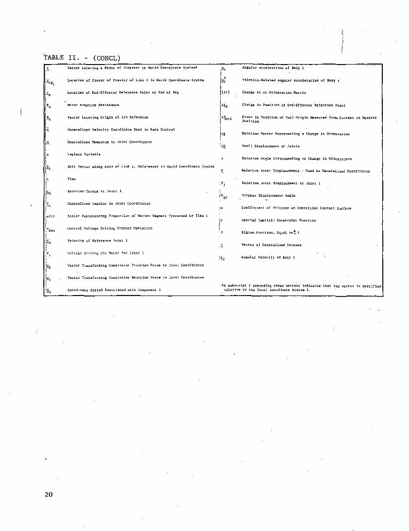
TABLE II. - (CONCL)
u( t )
Vector Locating a Point of Interest in World Coordinate System*
Location of Center of Gravity of Link 1 In World Coordinate System
Location of End-Effector Reference Point or End of Peg
Motor Armature Resistance
Vector Locating Origin of ith Reference
Generalised Velocity Coordinate Used in Rate Control
Generalized Momentum in Joint Coordinates
Laplace Variable
Unit Vector along Axis of Link i, Referenced to World Coordinate Syste:
Time
Reaction Torque at Joint 1
Generalized Impulse in Joint Coordinates
Scalar Representing Proportion of Motion Segment Traversed by Time t
Control Voltage Driving Gripper Operation
Velocity of Reference Point i
Voltage Driving the Meter for Joint i
Vector Transforming Constraint Friction Force to Joint Coordinates
Vector Transforming Constraint Reaction Force to Joint Coordinates
Coordinate System Associated with Component i
o^ Angular Acceleration of Body i
o^ Velocity-Related Angular Acceleration of Body i
[fip] Change In an Orientation Matrix
ir,, Change in Position of End-Effector Reference Point
Error In Position of Tool Origin Measured frotn Current to DesiredPosition
Rotation Vector Representing a Change in Orientation
Small Displacement of Joints
Rotation Angle Corresponding to Change in Orientation
Relative Joint Displacements - Used As Generalized Coordinates
Relative Joint Displacement at Joint i
Gripper Displacement Angle
Coefficient of Friction at Constraint Contact Surface
Special Implicit Constraint Function
Signum Function, Equal toil
Vector of Generalized Torques
Angular Velocity of Body i
.*A subscript I preceding these vectors Indicates that the vector Is specifiedrelative to the local coordinate system 1.
20
Kinematic Analysis
The kinematic and dynamic analysis tools implemented in ROBSIM are basedon a rigid-link model of serial, open-loop kinematic chains with one-degree-of-freedom joints. This subsection first describes the forward kinematics solu-tion. This is, given the vector & of relative joint displacements and theirfirst and second time derivatives (£, Q) for a specified arm geometry, find thepositions, orientations, velocities and accelerations of all links and pointsof interest in the device. Then methods for generating the time trajectoriesof the joint displacements (j)(t), £(t), £(t)), particularly for providing task-oriented operation of the manipulator, are discussed.
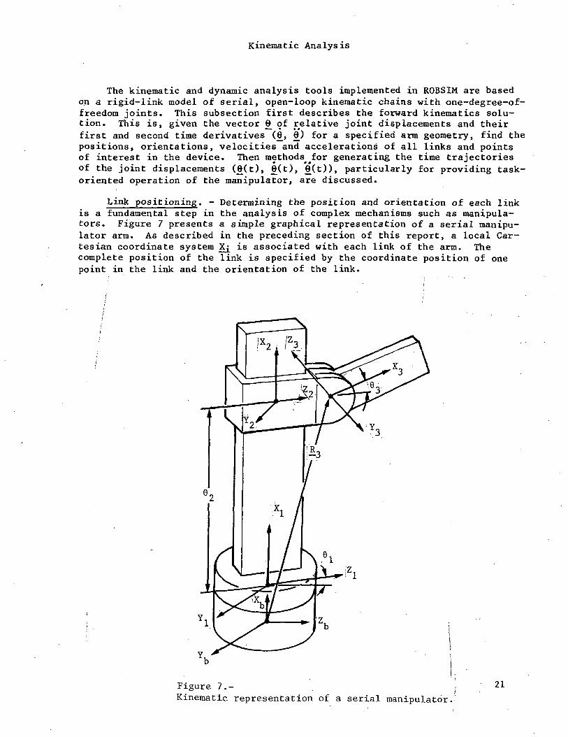
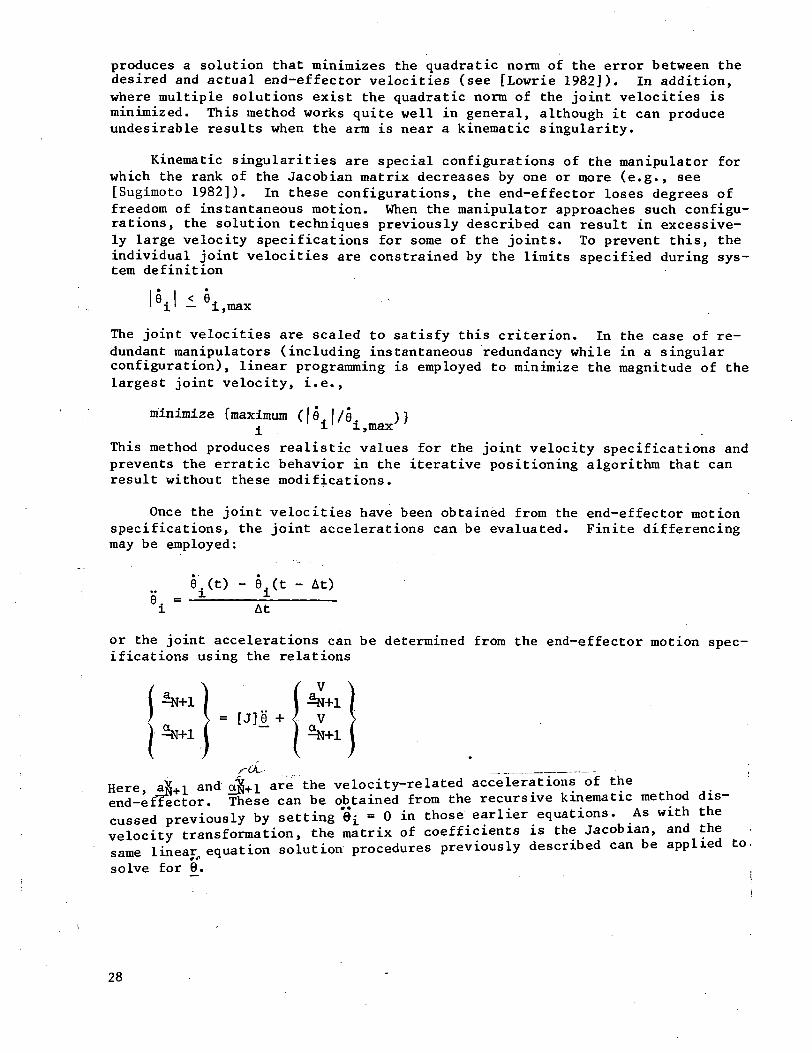
Link positioning. - Determining the position and orientation of each linkis a fundamental step in the analysis of complex mechanisms such as manipula-tors. Figure 7 presents a simple graphical representation of a serial manipu-lator arm. As described in the preceding section of this report, a local Car-tesian coordinate system X^ is associated with each link of the arm. Thecomplete position of the link is specified by the coordinate position of onepoint in the link and the orientation of the link.
Figure 7.-Kinematic representation of a serial manipulator.-
21
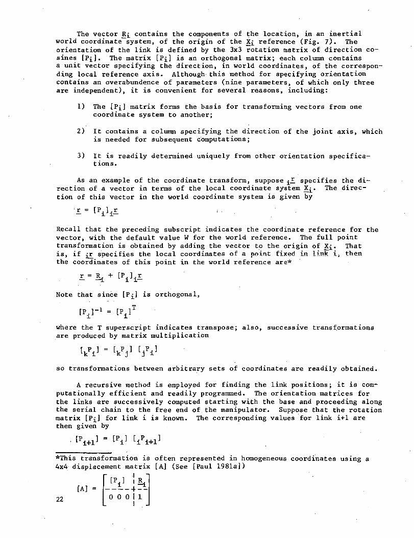
The vector R£ contains the components of the location, in an inertialworld coordinate system, of the origin of the X£ reference (Fig. 7). Theorientation of the link is defined by the 3x3 rotation matrix of direction co-sines [Pj_]. The matrix [Pf] is an orthogonal matrix; each column containsa unit vector specifying the direction, in world coordinates, of the correspon-ding local reference axis. Although this method for specifying orientationcontains an overabundence of parameters (nine parameters, of which only threeare independent), it is convenient for several reasons, including:
1) The [Pi] matrix forms the basis for transforming vectors from onecoordinate system to another;
2) It contains a column specifying the direction of the joint axis, whichis needed for subsequent computations;
3) It is readily determined uniquely from other orientation specifica-t ion s .
As an example of the coordinate transform, suppose, jJL specifies the di-rection of a vector in terms of the local coordinate system X^. The direc-tion of this vector in the world coordinate system is given by
Recall that the preceding subscript indicates the coordinate reference for thevector, with the default value W for the world reference. The full pointtransformation is obtained by adding the vector to the origin of Xi. Thatis, if ,£ specifies the local coordinates of a point fixed in link i> thenthe coordinates of this point in the world reference are*
Note that since [P ] is orthogonal,
[P.]-1 = [P±]T
where the T superscript indicates transpose; also, successive transformationsare produced by matrix multiplication
so transformations between arbitrary sets of coordinates are readily obtained.
A recursive method is employed for finding the link positions; it is com-putationally efficient and readily programmed. The orientation matrices forthe links are successively computed starting with the base and proceeding alongthe serial chain to the free end of the manipulator. Suppose that the rotationmatrix [PjJ for link i is known. The corresponding values for link i+1 arethen given by
*This transformation is often represented in homogeneous coordinates using a4x4 displacement matrix [A] (See [Paul 1981a])
[A] =22 0 0 0 I 1
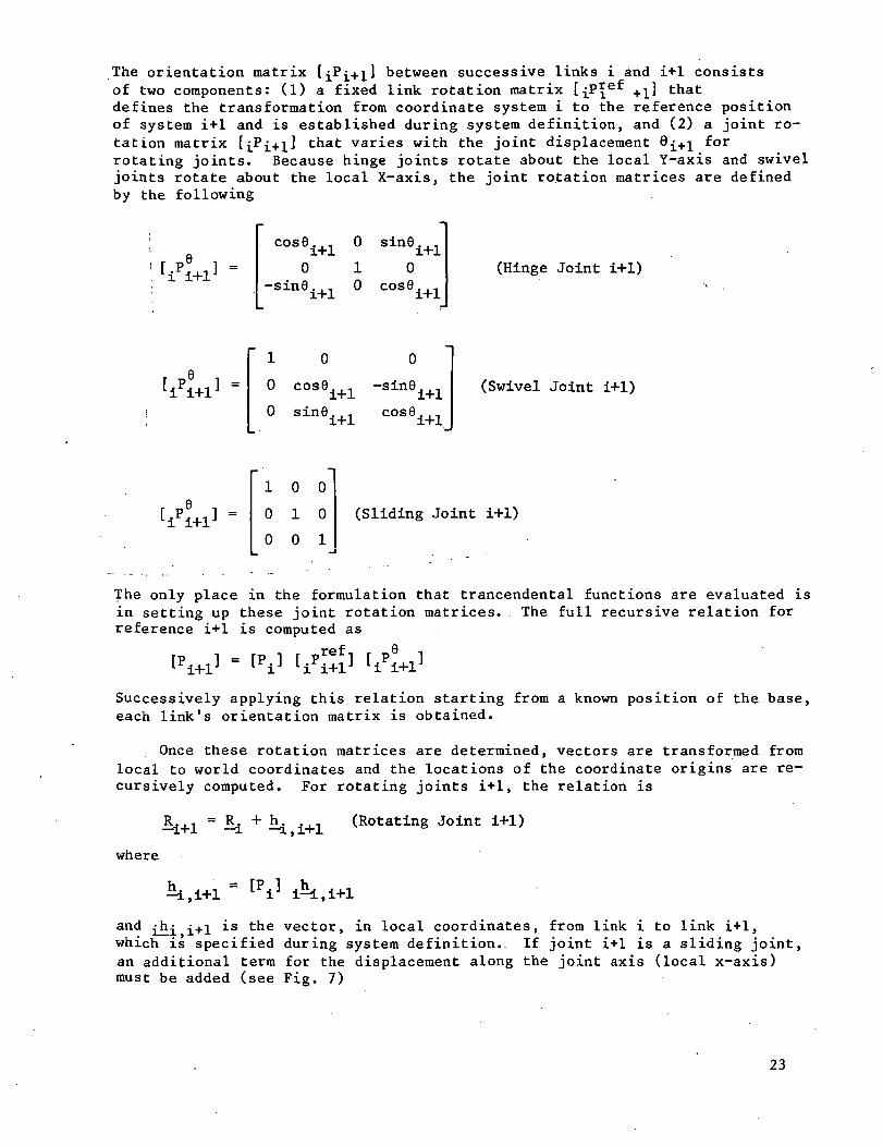
The orientation matrix tiPi+il between successive links i and i+1 consistsof two components: (1) a fixed link rotation matrix [jPl[ef +^1 thatdefines the transformation from coordinate system i to the reference positionof system i+1 and is established during system definition, and (2) a joint ro-tation matrix [£?!+]_] that varies with the joint displacement 0£+i forrotating joints. Because hinge joints rotate about the local Y-axis and swiveljoints rotate about the local X-axis, the joint rotation matrices are definedby the following
cOS0
-sine.+1
0i+10 1
o(Hinge Joint i+1)
1 0
0 cos0 .
0 sine. .,
0
L -Sin9i+l. cose. .
(Swivel Joint i+1)
1 0 0
0 1 0
0 0 1
(Sliding Joint i+1)
The only place in the formulation that trancendental functions are evaluated isin setting up these joint rotation matrices. The full recursive relation forreference i+1 is computed as
* T rp l r *"» ® n r T* ^— I"• J I •
Successively applying this relation starting from a known position of the base,each link's orientation matrix is obtained.
Once these rotation matrices are determined, vectors are transformed fromlocal to world coordinates and the locations of the coordinate origins are re-cursively computed. For rotating joints i+1, the relation is
" (Rotating Joint i+1)
where
and .jh.; £+1 is the vector, in local coordinates, from link i to link i+1,which is specified during system definition., If joint i+1 is a sliding joint,an additional term for the displacement along the joint axis (local x-axis)must be added (see Fig. 7)
23
ei+10
0
(Sliding Joint i+1)
Again, successive application of these recursive relations yields the locationof each local coordinate reference.
Note that once the position of each link's reference X^ is available,the world coordinates for any point in the link can be found using the pointtransformation given earlier. For example, i_£Cgi represents the localcoordinates of the centroid of link i and is established during system defi-nition. The instantaneous location of this centroid in terms of the world re->ference is given by
r = R. + [Pj .r,-cgi -i i i-cgj,
Link and point velocities. - The velocity of a rigid body is convenientlyspecified as the translational velocity of some point in the body along withthe angular velocity of the body. A recursive method based on classical rigid-body kinematics is employed to calculate the velocities and accelerations ofthe individual manipulator links. The method has received much attention in jthe recent literature on manipulator dynamics (e.g., see [Orin 1979], [Luh i1980], [Walker 1982]), and was chosen for its .efficiency, simplicity, and ease]of programming. !tf ,.|/ • •' }
Let o>£ represent the angul/ar velocity/of link i referenced to the worldcoordinate system. Assuming w^ is known,/the angular velocity <^i+i of thenext link is readily given as the sum of w^ plus the angular veTocity of linki+1 relative to link i, i+i/i- If joint i+1 is a rotating joint, then thisrelative angular velocity is a vector of magnitude 0£+i about the axis ofrotation, i.e., /
-i+l/i = 9i+l i+1 (Rotating Joint i+1)
Here, £i+i is a unit vector along the joint axis and is given in terms of thelink's orientation as
/ \0
(Hinge Joint i+1)
(Swivel or Sliding Joint i+1)
24
Therefore, starting with the specified angular velocity for the base, the angu-lar velocity of each link is obtained by successive application of the recur-sion relations
-i+1 = L + Vl i+1 (Rotating Joint i+1)
u. (Sliding Joint i+1)
Subsequently, the translational velocity \£i+l of the origin of thereference can be represented in terms of the translational and rotation-
al velocities of link i. If joint i+1 is a rotational joint, the relation is
V± + u^ x (R - 1) (Rotating Joint i+1)
while an additional term must be included for the sliding joint case
= V. + at. x (R±+1 - R^ + 6i+1 S (Sliding Joint i+1)
Recall that the vector from joint i to joint i+1, which is used in the vectorcrossproduct term in these equations, is given by
- R- = *L ., .1 (Rotating Joint i+1)— i — i , i+1
- *<. - h*. i+i + 8i+i Si+l (Sluing Joint- i+1)
In addition, if the velocity \/~ of any point P fixed in link i is desired, itis then obtained from
Vp - + OK x (^ - R^
For a specified velocity V^ of the manipulator base, the application of theseformulas provides values for the velocities of each link and all points of in-terest directly from the position results.
Link and point accelerations. - In a similar manner, the accelerations ofthe manipulator links can be solved for by recursive application of the second-order motion derivatives for rigid bodies. Let laj_ represent the angular ac-celeration of link i and a.£ the translational acceleration of the correspon-ding reference origin. The acceleration equations are as follows:
-i+1 = L + % x 9i+1 S +1 + 0±+1 S±+1 (Rotating Joint i+1)
-i+1 = % (Sliding Joint i+1)
25
a. , = a. + a), x [UK x (R... - R.)] + a. x (R - - R.) (Rotating Joint i+1)— i+1 — i — i —a. —i+1 — i — i — ITJ. — i
V ] + °LL x
6i+1 S^ + 0i+1 S (Sliding Joint i+1)
Again, the accelerations ajj and ojj of the base are presumed known, and theacceleration £p of any point of interest in link i can be readily obtained:
In particular, the acceleration £cgi of each link's centroid is calculatedfor use in the subsequent dynamic analysis.
Note that all vectors used in the preceding equations are expressed interms of the world reference system. Any other coordinate selection is poss-ible; the only constraint is that; a consistent set of coordinates must be usedthroughout each equation.
End-effector .motion. - While the kinematics and dynamics of serial manip-ulators are most conveniently evaluated in terms of the joint displacements andrates, it is often more useful to prescribe the motion of the terminal link("end-effector," "tool." or "hand") of the device, especially for task-orientedoperation. The algorithms employed in the ROBSIM package for transforming end-effector motion specifications into joint motion states are described here.
The inverse positioning problem, that of finding a set of joint displace-ments j) corresponding to a prescribed end-effector position can be exceedinglycomplex* and analytic solution methods are not readily generalizable. However,commercial robots generally have special geometries, resulting in much simplerpositioning solutions (e.g., see [Duffy 1979], [Paul 1981b]). Special routinescan be programmed for certain geometries or classes of geometries. For gener-ality, an iterative positioning routine is implemented in ROBSIM; because itinvolves an extension of the velocity results, it is described after the velo-city relations are presented.
i _ -i *For example, the solution for a six-degree-of-freedom arm can involve finding
roots to a polynomial of up to 32nd order (see [Duffy 1981], [Duffy 1980]).Methods for analytically handling the positioning of redundant manipulators arenot even available.
26
A method for recursively computing the end-effector velocity from thejoint rates was described previously. For a given position & of the manipula-tor, the velocity (Vjj+j , OJN+I) of the end-effector link N+l can also bewritten explicity in terms of the joint velocities as
[jce)i i <*)
Here, [J(9)J is the Jacobian matrix relating the end-effector motion to jointmotion. Column i of the 6xN matrix [J] is readily expressed in terms of theposition results as follows (see [Whitney 1972], [Thomas 1982]):
J. = (Rotating Joint i)
-i (sliding Joint i)
(The motion of some reference point other than the tool reference origin canbe used by replacing Vjj+ and E +i by \fp
anc^ £n in these equations.)
For a specified end-effector velocity, Eq. (*) above represents a simul-taneous set of six scalar equations linear in the N unknown joint velocities0£. These equations will result in either a unique solution, an infinitenumber of solutions, or no exact solutions; they can be solved by standardtechniques of linear algebra. For example, using the pseudo-inverse ~^of the Jacob ian
[J]-i*
27
produces a solution that minimizes the quadratic norm of the error between thedesired and actual end-effector velocities (see [Lowrie 1982]). In addition,where multiple solutions exist the quadratic norm of the joint velocities isminimized. This method works quite well in general, although it can produceundesirable results when the arm is near a kinematic singularity.
Kinematic singularities are special configurations of the manipulator forwhich the rank of the Jacobian matrix decreases by one or more (e.g., see[Sugimoto 1982]). In these configurations, the end-effector loses degrees offreedom of instantaneous motion. When the manipulator approaches such configurations, the solution techniques previously described can result in excessive-ly large velocity specifications for some of the joints. To prevent this, theindividual joint velocities are constrained by the limits specified during system definition
The joint velocities are scaled to satisfy this criterion. In the case of re-dundant manipulators (including instantaneous redundancy while in a singularconfiguration), linear programming is employed to minimize the magnitude of thelargest joint velocity, i.e.,
minimize (maximum (1 6.1/6 )}^ i ' i ,max
This method produces realistic values for the joint velocity specifications andprevents the erratic behavior in the iterative positioning algorithm that canresult without these modifications.
Once the joint velocities have been obtained from the end-effector motionspecifications, the joint accelerations can be evaluated. Finite differencingmay be employed:
ei =9i(t) ~ 8i(t " At)
At
or the joint accelerations can be determined from the end-effector motion spec-ifications using the relations
V•%+!V
Here aX+i and ol+i are the velocity-related accelerations of theend-effector. These can be obtained from the recursive kinematic method dis-cussed previously by setting "0'i = 0 in those earlier equations. As with thevelocity transformation, the matrix of coefficients is the Jacobian, and thesame linear, equation solution procedures previously described can be applied to.
solve for 9.
28
Returning to the problem of finding the joint positions £ for a prescribedend-effector position, an iterative method is implemented in ROBSIM. The al-gorithm uses the solution of a set of linear equations, where the Jacobianagain forms the coefficient matrix, and is described in [Whitney 1972]. Basedon the current position and desired position of the end-effector, a six-dimensional position error vector is obtained. This error vector is used tosolve for a vector of joint corrections ,Aj9. from
Rjy+i is the translational position error and .A $ represents a rotationvector (the magnitude gives the angle of rotation and the direction specifiesthe axis) that rotates the end-effector from the current to the desired orien-tation. A method for solving for the vector jA^ is described in the next sub-section. Applying the special solution methods previously discussed allows li-mits to be placed on the size of the change (A9_£ in the joint angles. Thisimproves convergence of the positioning method for large initial errors or whenoperating near singularities.
After solving for,A0^ the joint displacements are updated,
6 = 6 , , + A9-new -old —
the current end-effector position is recalculatedj and the process is repeateduntil the end—effector position converges to the desired value. Because thisis an iterative method, only a single position solution will result (dependingon the initial values of &), although the manipulator geometry may have multi-ple configurations corresponding to the same end-effector position. To date,testing has shown the method to be quite robust as long as reasonable limits(e.g., 0.1 radian) are placed on the changes in joint displacement per iter-ation step.
Task-oriented motion specification. - This section has presented methodsfor determining link motions from joint motion states and for finding joint mo-tions that produce end-effector trajectories. To make task programming moreconvenient, a user-interface is implemented that allows interactive specifica-tion of a sequence of operations and robot motions. The motions generated fromthese specifications are described in the following paragraphs.
The overall task specification is divided into motion segments. The fol-lowing options are available for defining the motion within each individualtime segment:
1) Rate control,a) Joint motion,b) End-effector motion (world coordinates and local end-effector
coordinates);
2) Position control,a) Joint motion,b) End-effector motion (world coordinates).
29
For rate control motion, the velocities of the individual position coordi-nates are specified as polynominal functions of time
4 = a t + a , t + . . . + a- 1 + a~
where q is the rate of some position component and the a^ are user-specifiedcoefficients. For rate. control of joint motion, q corresponds to the indivi-dual joint velocities, 0£. Therefore, the joint velocities at any time dur-ing the segment are determined by evaluating the rate polynomials for the giventime, t. Furthermore, the polynomials can be symbolically differentiated andthe joint accelerations found by evaluating
The joint displacements are updated using Euler integration of the velocityresults*
Q± (t + At) = ei(t) + At * e t)
When rate control of end-effector motion is specified, the q polynominalscorrespond to the six components of end-effector velocity, Vp and
(A different tool reference point P can be used for each motion segment.) Attime t, the rate polynominals are evaluated to determine the end-effector ve-locity. These velocity vectors can be defined in either world coordinates orinstantaneous end-effector coordinates. If defined in local end-effector coordinates, the vectors are transformed into world coordinates by premultiplyingeach by [PN+]J . The joint velocities are then solved for using the Jacobianinversion method described previously. The joint accelerations are obtainedfrom these velocities using the backwards finite-differencing equations, andthe joint displacements are evaluated, as before, from the Euler integrationequation.
Position control segments provide coordinated motion between user-specified trajectory endpoints. Each position component is scaled so they allreach their final values simultaneously. For example, for joint position con-trol, the initial joint displacements 6_(to) are known from the manipulator'scurrent location and the final displacements 6(tf) are specified. The jointpositions at any intermediate time during the motion segment are then given by
£(t) = e.(tQ) + u(t) A9_
where
A = ^ >
^Although symbolic integration of the rate polynomial could be used for thiscase, the Euler integration method must be employed for the end-effector ratecontrol specification.
30
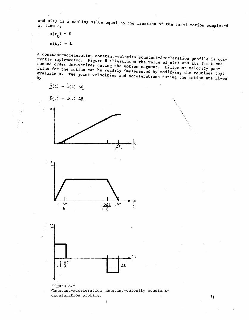
t0 the fracti°* °f the total nation- completed
u(t0) = 0
u(tf) = 1
-*
u(t) A9
and accelerations during the motion are given
9(t) = U(t) A6
u •j
Ui
At6
'5At SAt! 6 l
! AtAt
Figure 8.-Constant-acceleration constant-velocity constant-deceleration profile. 31
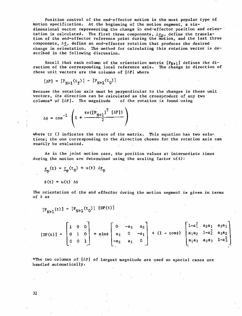
Position control of the end-effector motion is the most popular type ofmotion specification. At the beginning of the motion segment, a six-dimensional vector representing the change in end-effector position and orien-tation is calculated. The first three components, .Ar_p, define the transla-tion of the end-effector reference point during the motion, and the last threecomponents, A£, define an end-effector rotation that produces the desiredchange in orientation. The method for calculating this rotation vector is de-scribed in the following discussion.
Recall that each column of the orientation matrix [PN+].] defines the di-rection of the corresponding local reference axis. The change in direction ofthese unit vectors are the columns of [Ap] where
CAP1 = tPN+l(tf)] - [PN+l(tO)]
Because the rotation axis must be perpendicular to the changes in these unitvectors, its direction can be calculated as the crossproduct of any twocolumns* of [AP]. The magnitude of the rotation is found using
A<J> = cos-1 1 +
tr([PN+l][AP])
where tr () indicates the trace of the matrix. This equation has two solu-tions; the one corresponding to the direction chosen for the rotation axis canreadily be evaluated.
As in the joint motion case, the position values at intermediate timesduring the motion are determined using the scaling factor u(t):
Ct) +u(t) Ar
<Kt) = u(t) A<f>
The orientation of the end effector during the motion segment is given in termsof 4" as
[DP(t)] =
1 0 0
0 1 0
0 0 1
sin<f>
-a2
-a3 a2
0 -al
a 0
- cos<())
l-af
1-ai
a2a3
a3a2
1-1
*The two columns of [AP] of largest magnitude are used so special cases arehandled automatically.
32
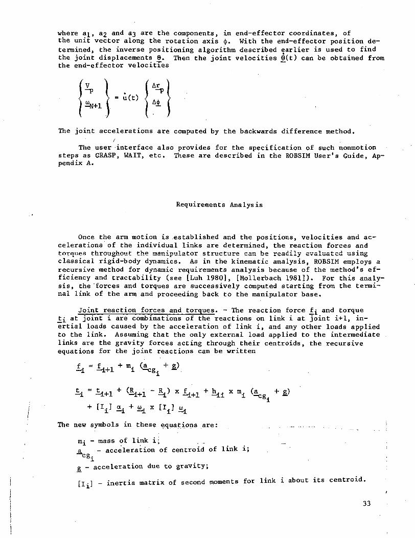
where a]_, a£ and 33 are the components, in end-effector coordinates, ofthe unit vector along the rotation axis cj>. With the end-effector position de-termined, the inverse positioning algorithm described earlier is used to findthe joint displacements 0. Then the joint velocities (J(t) can be obtained fromthe end-effector velocitTes
V Ar-P
The joint accelerations are computed by the backwards difference method./
The user interface also provides for the specification of such nonmotionsteps as GRASP, WAIT, etc. These are described in the ROBSIM User's Guide, Ap-pendix A.
Requirements Analysis
Once the arm motion is established and the positions, velocities and ac-celerations of the individual links are determined, the reaction forces andtorques throughout the manipulator structure can be readily evaluated usingclassical rigid-body dynamics. As in the kinematic analysis, ROBSIM employs arecursive method for dynamic requirements analysis because of the method's ef-ficiency and tractability (see [Luh 1980], [Hollerbach 1981]). For this analy-sis, the'forces and torques are successively computed starting from the termi-nal link of the arm and proceeding back to the manipulator base.
Joint reaction forces and torques. - The reaction force and torqueJ:^ at joint i are combinations of the reactions on link i at joint i+1, in-ertial loads caused by the acceleration of link i, and any other loads appliedto the link. Assuming that the only external load applied to the intermediatelinks are the gravity forces acting through their centroids, the recursiveequations for the joint reactions can be written
- RJ x f.+. + h. x m (a o + j»)
+ [I.] c^ 4- x [I±]
The new symbols in these equations are:
mj^ - mass of link i^.a. - acceleration of centroid of link i;
"Cgig - acceleration due to gravity;
[IL] - inertia matrix of second moments for link i about its centroid.
33
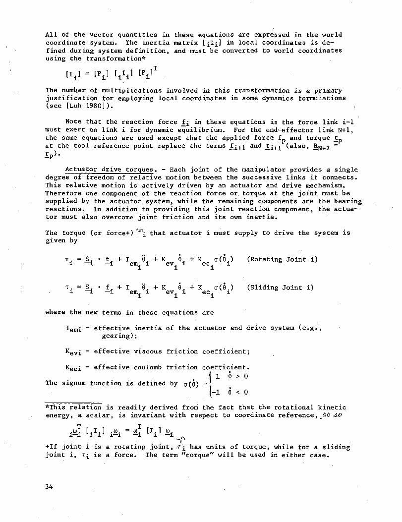
All of the vector quantities in these equations are expressed in the worldcoordinate system. The inertia matrix [£!]_] in local coordinates is de-fined during system definition, and must be converted to world coordinatesusing the transformation*
[I.] = [P.] [ 1 I*/
The numb.er of multiplications involved in this transformation is a primaryjustification for employing local coordinates in some dynamics formulations(see [Luh 1980]).
Note that the reaction force in these equations is the force link i-1must exert on link i for dynamic equilibrium. For the end-effector link N+l,the same equations are used except that the applied force £ and torque ^pat the tool reference point replace the terms i+i and ££+•[ (also, Rjj+2 =
£p).
Actuator drive torques. - Each joint of the manipulator provides a singledegree of freedom of relative motion between the successive links it connects.This relative motion is actively driven by an actuator and drive mechanism.Therefore one component of the reaction force or torque at the joint must besupplied by the actuator system, while the remaining components are the bearingreactions. In addition to providing this joint reaction component, the actua-tor must also overcome joint friction and its own inertia.
The torque (or force+) \ that actuator i must supply to drive the system isgiven by
T. = S. • t. + I 6, + K 6. + K a(9.) (Rotating Joint i)i —i —i em. i ev. i ec i 6
T- = .§• f, + I 9.+K 9. + K a(0J (Sliding Joint i)i -1 —i enu i ev.j i ec± i 6
where the new terms in these equations are
Iemi ~ effective inertia of the actuator and drive system (e.g.,gearing);
Kev£ - effective viscous friction coefficient;
Kec£ - effective coulomb friction coefficient.
The signum function is defined by a(9)
Wl* l V .1- J. J.V«Jk
( 1 6 > 0'in =/
(-1 e < o
*This relation is readily derived from the fact that the rotational kineticenergy, a scalar, is invariant with respect to coordinate reference, ,so ,&<&
+If joint i is a rotating joint, ,t\ has units of torque, while for a slidingjoint i, i^ is a force. The term "torque" will be used in either case.
34
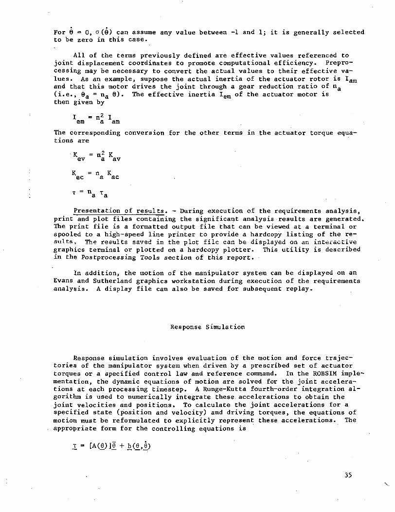
For 9 = 0, .o (9) can assume any value between -1 and 1; it is generally selectedto be zero in this case.
All of the terms previously defined are effective values referenced tojoint displacement coordinates to promote computational efficiency. Prepro-cessing may be necessary to convert the actual values to their effective va-lues. As an example, suppose the actual inertia of the actuator rotor is Iamand that this motor drives the joint through a gear reduction ratio of nfl(i.e., 9a = na 6). The effective inertia Iem of the actuator motor isthen given by
I = n2 Iem a am
The corresponding conversion for the other terms in the actuator torque equa-tions are
K = n2 Kev a av
K = n Kec a ac
T = n Ta a
Presentation of results. - During execution of the requirements analysis,print and plot files containing the significant analysis results are generated.The print file is a formatted output file that can be viewed at a terminal orspooled to a high-speed line printer to provide a hardcopy listing of the re-sults, The results saved in the plot file can be displayed on an interactivegraphics terminal or plotted on a hardcopy plotter. This utility is describedin the Postprocessing Tools section of this report.
In addition, the motion of the manipulator system can be displayed on anEvans and Sutherland graphics workstation during execution of the requirementsanalysis. A display file can also be saved for subsequent replay.
Response Simulation
Response simulation involves evaluation of the motion and force trajec-tories of the manipulator system when driven by a prescribed set of actuatortorques or a specified control law and reference command. In the ROBSIM imple-mentation, the dynamic equations of motion are solved for the joint accelera-tions at each processing timestep. A Runge-Kutta fourth-order integration al-gorithm is used to numerically integrate these accelerations to obtain thejoint velocities and positions. To calculate the joint accelerations for aspecified state (position and velocity) and driving torques, the equations ofmotion must be reformulated to explicitly represent these accelerations. Theappropriate form for the controlling equations is
T =
35
where _r is the vector of actuator driving torques, [A(6)j is the effective in-ertia matrix referenced to joint coordinates, and _b(8 ,£) is a vector ofposition- and velocity-related effective torques. The calculation of theseterms is described in the following subsections.
Actuator driving torques. - The actuator torques driving the response sim-ulation can be generated by one of the following methods:
1) Read a file of actuator torques versus time;
2) Read a file of actuator voltages versus time;
3) Use a feedback control law.
The first of these methods can be used to determine response to specific torquecommand profiles, such as a sinewave input. Alternately, an actuator torquefile generated during a requirements analysis run could subsequently be used todrive the response simulation, thereby providing validation that the require-ments analysis and response simulation agree.
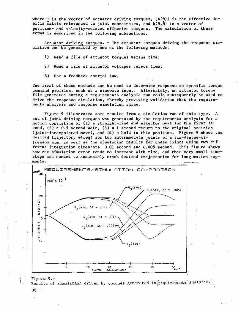
Figure 9 illustrates some results from a simulation run of this type. Aset of joint driving torques was generated by the requirements analysis for amotion consisting of (1) a straight-line end-effector move for the first se-cond, (2) a 0.5-second wait, (3) a 1-second return to the original position(joint-interpolated move), and (4) a hold in this position. Figure 9 shows thedesired trajectory 0(req) for two intermediate joints of a six-degree-of-freedom arm, as well as the simulation results for these joints using two dif-ferent integration timesteps, 0.01 second and 0.005 second. This figure showshow the simulation error tends to increase with time, and that very small time-steps are needed to accurately track desired trajectories for long motion seg-ments. __. ,
, REQUTREMENTS/SIMULRTION COMPHRISON
, At = .005)
10 15 20TXME [SECONDS!
30 .«i<r'
Figure 9.- _ , . ,Results of simulation driven by torques generated in [requirements analysis.
36
Actuation methods 2) and 3) are used with the dc torque-motor model imple-mented in ROBSIM. The torque supplied by motor i is proportional to the arma-ture current i^:
T. = K ^ i.i et. i
where Ket^ is the effective torque constant of the motor. The armature cur-rent is a function of the applied voltage Vj^
di.__ T 3 - L - n 3 J, V ft
where L^ is the armature inductance, Ra£ is the armature resistance and^emfi ^-s t*ie errective back-emf coefficient for the motor. In the motors mo-deled to date, the armature inductance has been found to be so small (hence,the electrical time constant is very short) that an unrealistically small in-tegration timestep is required to track the electrical dynamics of the motor.Therefore, the inductance is neglected in the current motor model and the torque can be related to the applied voltage by combining the above equations toobtain
V. - K . 6.i emf . i
In this equation, all coefficients are referenced to the joint displace-ments coordinates <9. If, for example, the gear reduction ratio is na, theeffective values are related to the actual motor coefficients Kat and Kaemfby
K. = n K _et a at
; K f = n K .emf a aemf
If a voltage file is read, equation (*) is then used to compute the actuatordriving torque at each timestep. At intermediate times for which no voltagehas been saved in the voltage file, linear interpolation is used to determinethe voltage value.
Rather than reading a previously established file of command voltages, the ,motor drive voltages can be generated during the simulation run using a feed- ,back control law. The implementation of feedback control models in the ROBSIM ;program is discussed in a subsequej^_s_ectjLcin_on maniBuia.tor_..,c.ontrollers. '
. ^ jPosition- and velocity-related torques. - The vector ]>(£•,£•) of position-
and velocity-related torques (see bottom of page 35) includes The effects ofstatic loads (such as gravity and applied forces), friction, and the velocity-related inertia terms ("centripetal" and "Coriolis" torques). Because this :
effective torque contribution depends on the current manipulator state and in-cludes all torque terms except the inertia torques attributable to joint accel-erations, the vector b_ is conveniently and efficiently computed by performing
37
the requirements analysis with the joint accelerations £ set to zero. There-fore no additional program modules need to be implemented for the evaluation ofthis term.
Effective inertia matrix. - The matrix [A(4J-)] of position-dependent in-ertia coefficients provides the relation between joint accelerations and actua-tor torques, including dynamic crosscoupling (i.e., acceleration at joint iproduces reaction torques at the other joints). This matrix is symmetric andpositive-definite; the kinetic energy of the manipulator in motion is given bythe quadratic form
i K.E.
An efficient algorithm for calculating the inertia matrix, based on the resultsin [Thomas 1982] and [Walker 1982], is implemented in the ROBSIM package. Abrief presentation of the equations used is given below.
Consider link i of the manipulator with mass m^, centroid location£.cgi an<^ inertia distribution [Ijj (in the current configuration). The ef-fective inertia [A1] due to this link's mass distribution is given by
[A1] -
[M±]
[J ]
and where [M^l is a 3y3 diagonal matrix with the link mass M^ along thediagonal^and where [J ] can be written
*s.-J
(Rotating Joint j<i)
J1—J
S.-J
000
(Sliding Joint j<i)
For j „> i, the components of J_i are zero because displacement at joint jhas no effect on the absolute motion of link i. The total inertia matrix isobtained by summing the contributions from each link i. The efficiency of thealgorithm is further improved by using the symmetry of [A] to reduce the numberof terms calculated. Also, composite masses, centroids and inertias consisting
38
of the mass of all links from joint i to the free end of the arm are computedfor each i. This allows each term of the expression for [A] to be evaluatedfor only one composite mass instead of for each individual link's mass (see[Walker 1982]).
The mass and inertia of a load being carried by the manipulator are in-cluded in the matrix of inertia coefficients by adding them to the mass distri-bution of the end-effector. In addition, the effective inertia, Iemi> °factuator i is added to the ith diagonal term of [A].
Because the effective inertia matrix is positive-definite, the equationsof motion
T_ •= [A (6) 11 + b.(l,l)
can be solved uniquely to obtain £ in terms of the state ( ,) and driving tor-ques _T.
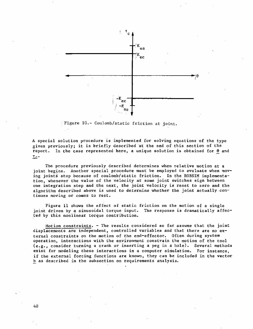
Joint friction. - As discussed in the Requirements Analysis section, twotypes of joint friction—viscous and coulomb—are implemented. The viscousfriction is readily included in the torque vector .b(j),j)) as is the coulombfriction as long as the joint velocity is not zero. Special methods for hand-ling the coulomb friction term must be employed when the velocity 0£ at somejoint is zero.
Figure 10 shows the joint coulomb friction TC as a function of joint ve-locity. This figure illustrates that when the joint velocity is zero, the cou-lomb friction torque value is not uniquely defined, but lies somewhere betweenthe minimum and maximum values -Kes and Kes, where Kes is the effectivestatic friction coefficient for the joint. In the case when one or more jointshave zero velocity, the set of equations to be solved for the joint accelera-tions can be written
[A (6) ]0. = jr - ;b(6,1) + T
-K < T < KesjL- c±- es.
where T_C is the vector of joint friction torques for the zero-velocityjoints, and the selection function p has the special definition
p(c,x ,x ) =
x ; c<0
+x ; c>0
x (arbitrary); c=0
39
-Kec'<es
esIK; ec
Figure 10.- Coulomb/static friction at joint.
A special solution procedure is implemented for solving equations of the typegiven previously; it is briefly described at the end of this section of thereport. In the case represented here, a unique solution is obtained for 9 andT_c.
The procedure previously described determines when relative motion at ajoint begins. Another special procedure must be employed to evaluate when mov-ing joints stop because of coulomb/static friction. In the ROBSIM implementa-tion, whenever the value of the velocity at some joint switches sign betweenone integration step and the next, the joint velocity is reset to zero and thealgorithm described above is used to determine whether the joint actually con-tinues moving or comes to rest.
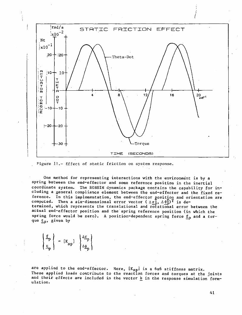
Figure 11 shows the effect of static friction on the motion of a singlejoint driven by a sinusoidal torque input. The response is dramatically affec-ted by this nonlinear torque contribution.
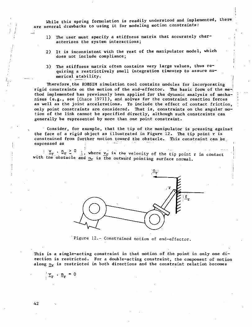
Motion constraints. - The results considered so far assume that the jointdisplacements are independent, controlled variables and that there are no ex-ternal constraints on the motion of the end-effector. Often during systemoperation, interactions with the environment constrain the motion of the tool(e.g., consider turning a crank or inserting a peg in a hole). Several methodsexist for modeling these interactions in a computer simulation. For instance,if the external forcing functions are known, they can be included in the vectorb_ as described in the subsection on requirements analysis.
40
;Ntixio
jrad/s
|xlO
-1
STHTIC FRICTION
J20-- J20--
I-20- -20--
-30 -- -Torque
TIME CSECONDS3
Figure 11.- Effect of static friction on system response.
One method for representing interactions with the environment is by aspring between the end-effector and some reference position in the inertialcoordinate system. The ROBSIM dynamics package contains the capability for in-cluding a general compliance element between the end-effector and the fixed re-ference. In this implementation, the end-effector position and orientation arecomputed. Then a six- dimensional error vector ( Arl;, ., . is de-termined, which represents the translational and rotational error between theactual end-effector position and the spring reference position (in which thespring force would be zero). A position-dependent spring force fp and a tor-que _tp, given by ~
f-P
t-P
sp
Ajc
A
are applied to the end-effector. Here, [Ksp] is a 6x6 stiffness matrix.These applied loads contribute to the reaction forces and torques at the jointsand their effects are included in the vector _b in the response simulation form-ulation.
41
While this spring formulation is readily understood and implemented, thereare several drawbacks to using it for modeling motion constraints:
!
1) The user must specify a stiffness matrix that accurately char- |acterizes the system interactions; :
2) It is inconsistent with the rest of the manipulator model, which |does not include compliance; ;
i3) The stiffness matrix often contains very large values, thus re- ,
quiring a restrictively small integration timestep to assure nu-merical stability. i
Therefore(the ROBSIM simulation tool contains modules for incorporating jrigid constraints on the motion of the end-effector. The basic form of the me-jthod implemented has previously been applied for the dynamic analysis of mecha-nisms (e.g., see [Chace 1971]), and solves for the constraint reaction forcesas well as the joint accelerations. To include the effect of contact friction,only point constraints are considered. That is, constraints on the angular mo-tion of the link cannot be specified directly, although such constraints cangenerally be represented by more than one point constraint.
Consider, for example, that the tip of the manipulator is pressing againstthe face of a rigid object as illustrated in Figure 12. The tip point r isconstrained from further motion toward the obstacle. This constraint can be,expressed as ; '" <
nr - 0i . where v_ is the velocity of the tip point r in contact
t • . i . • . .. * *with the obstacle and nr is the outward pointing surface normal.
Figure 12.- Constrained motion of end-effector.
This is a single-acting constraint in that motion of the point in only one di-rection is restricted. For a double-acting constraint, the component of motionalong nr is restricted in both directions and the constraint relation becomes
nr 0
42
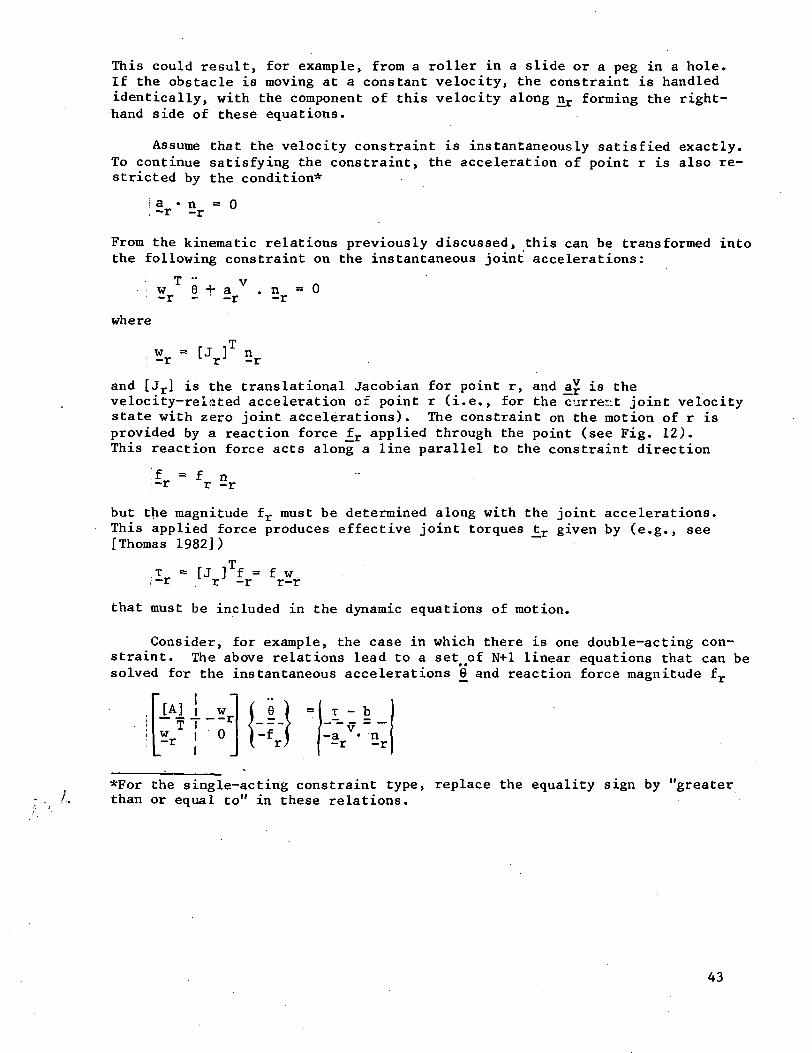
This could result, for example, from a roller in a slide or a peg in a hole.If the obstacle is moving at a constant velocity, the constraint is handledidentically, with the component of this velocity along n^ forming the right-hand side of these equations.
Assume that the velocity constraint is instantaneously satisfied exactly.To continue satisfying the constraint, the acceleration of point r is also re-stricted by the condition*
From the kinematic relations previously discussed, this can be transformed intothe following constraint on the instantaneous joint accelerations:
T v
where
w-r
t a
[J ]T n1 r -r
= 0
and [Jr] is the translational Jacobian for point r, and a£ is thevelocity-related acceleration of point r (i.e., for the current joint velocitystate with zero joint accelerations). The constraint on the motion of r isprovided by a reaction force fj. applied through the point (see Fig. 12).This reaction force acts along a line parallel to the constraint direction
'f « f n-r r -r
but the magnitude fr must be determined along with the joint accelerations.This applied force produces effective joint torques j r given by (e.g., see[Thomas 1982])
T = [J ]Tf = f W• -r r -r r-r
that must be included in the dynamic equations of motion.
Consider, for example, the case in which there is one double-acting con-straint. The above relations lead to a set^of N+l linear equations that can besolved for the instantaneous accelerations £ and reaction force magnitude fr
[A] w
w I 0
T - b
-a • n-r -r
*For the single-acting constraint type, replace the equality sign by "greaterthan or equal to" in these relations.
43
Configurations containing single-acting constraints can be handled by em-ploying the nonlinear, partial constraint function p defined previously in thesubsection on joint friction. In this case, the equations to be solved for thejoint accelerations and reaction force are:
[A] 0 = T - b + f r wr
fr I °
i w T 6: + a v • n > 0-r - -r -r -
: fr = P(wrT I + §/ ' -r' "' 0)
The implicit function p is introduced to represent the fact that the reactionforce must vanish as the point accelerates away from the constraint. (Notethat the conditional cannot be less than zero in this case.)
The solution procedure described at the end of this section is again em-ployed to solve these equations. In general, a unique solution will exist.However, if some joints have zero velocity and some constraints are active, thereaction force distribution may be indeterminate, although a unique set ofjoint accelerations will result. More than one motion constraint can be con-sidered simultaneously by simply expanding the set of equations.
Impact of collision. - In the above equations, it was assumed that thepoint velocity already satisfied the motion constraint. However, when thepoint initially collides with the obstacle, this will not be true. In the act-ual case, this collision will introduce oscillatory transients in the motion.This rapid transfer of momentum can be modeled as an inelastic collision to de-termine the velocity of the system after impact. To evaluate the joint veloci-ties after impact, consider the generalized momenta Q, which are given by
•
Q = [Ale
where [A] is the inertia matrix defined earlier. The change A £ in generalizedmomenta must equal the generalized impulse Tj that results from the impul-sive reactive force at the constraint. If the reaction impulse has magnitudefj, then the generalized impulse will be
Si * [J/ fl 5r - fx wr
This leads to a set of linear equations for determining the change A0 in thejoint velocities during the impact:
wAQ = TZ =^ [A] ae - f
44
Combining these equations with the fact that the velocity constraint must besatisfied after impact leads to the following set of equations for obtainingthe joint velocities after the collision
[A] I w A6 0
6 _ = e + A0• -after -before -
where v_r is the velocity of the constraint point before impact.
Coulomb friction at the constraint points. - In addition to the normal re-action force at the point of contact with the obstacle, there is also a fric-tion force tangent to the restraining surface. This friction force, ff, isproportional to the normal force and directed opposite to the tangential velo-city, i.e.,
where /i is the coefficient of friction and e^. is a unit vector in the di-rection of tangential motion of the constrained point relative to the surface.The effective torque contribution at the joints is again found by premulti-plying the friction force by the transpose of the Jacobian. For the single-acting constraint type, the equations are the same as given earlier, except th?term frWj- is replaced by where
| wf = LJ
rJ Sr
In the case of a double-acting constraint, slightly more modification isneeded because the magnitude of r can equal plus or minus fr. This caseis put into the standard form used above by replacing fr with two variablesf£ and f~, one of which is always zero depending on the sign of fr.The joint torque contribution from the reaction normal force and friction forcecan be written
-r = fr - fr~
(-r+y-f)
The additional constraints for this case are
f/ > 0
-f > 0
p(fr+, -, o)
where the selection function P implies that f^ = 0 if f£ > 0 andf~ has an arbitrary value (i.e., must be solved fom other constraints)
when f = 0.
45
As discussed for the joint friction case, the real difficulty in handlingcoulomb friction occurs at the singularity when the relative velocity betweenthe interacting surfaces is zero. However, the ability to simulate this caseis critical. For example, consider the insertion of a peg in a hole. It isvital to determine whether the insertion will proceed in the presence of cou-lomb friction, or whether the peg will instead jam in the hole. If jammingdoes occur, will the manipulator be able to free the peg and continue inser-tion?
To model the case of coulomb friction with zero tangential velocity, thefriction force is approximated by two mutually perpendicular forces
£f - vcc/ J/ + cr2 e/)
where e£ and e£ are two mutually perpendicular unit vectors that arealso perpendicular to the surface n9rmal (i.e., they define the instantaneoustangent plane). The coefficients c£ are bounded by the magnitude of thenormal force
c 1 + If I > 0r ' r' -
t
-c ± + |f | > 0; 1=1,2
Additionally, if the contact point has nonzero tangential acceleration, thefriction force will have its limiting magnitude so
and
/. |frl. - l*rl> : 1-1.2
r1 = <wfST 6 + a .e/ ; i-1,2
The magnitude of the normal force for the single- and double-acting constrainttypes for use in these relations is given by
. |f | = f (single-acting)
|f | = f + - f (double-acting)
This method introduces two additional unknowns (c£) and six additionalconstraints (four linear inequalities, two nonlinear partial constraints), allin the standard form developed previously. Some results using these equationsare presented in a subsequent section of the report.
46
Modeling the ISRL Multisensor End-Effector
One component of today's manipulators that is woefully inadequate comparedto the dexterity and sensitivity of its human counterpart is the manipulatorend-effector or hand. Advanced mission applications will surely require moresensing capabilities than employed in industrial robots, which typically haveat most a single presence detector, and more handling dexterity than the uncon-trolled opening and closing of simple pneumatic grippers. This section de-scribes the simulation of advanced end-effectors that incorporate several typesof internal and external sensing and controlled gripping actions and discussesa specific implementation—the microprocessor-controlled gripper/sensor systemdeveloped for and in use at the Intelligent Systems Research Laboratory (ISRL)at NASA-LRC. The end-effector consists of a parallel jaw gripper mechanismwith force sensors and proximity sensors mounted in the jaws and is attached tothe manipulator through a six-degree-of-freedom wrist force sensor. The simu-lation model includes the geometry and dynamics of gripper operation, influe-nces of load inertias on arm operation, wrist and jaw force sensors, and jaw-mounted proximity sensors.
Configuration of the ISRL end-effector. - Figure 13 displays the ISRL end-effector and Figure 14 illustrates the functional components of the gripper.The end-effector mechanical design and concept for proximity detection origi-nated at the University of Rhode Island. The body of the end-effector houses adc torque motor. A nylon gear on its shaft drives an incremental shaft encoderand a dc tachometer providing position and rate feedback; the gearing providesa 1:2.78 speed increase. The encoder output is wired directly into the micro-processor controller and the tachometer output is summed with the positionerror signal in the servoamplifier (Fig. 14). A limit sensor indicating the.fully open configuration of the jaws provides a reference for the incrementalposition encoders. A worm gear on the motor shaft drives two opposing sectorgears, each of which is attached to a link in a parallelogram mechanism thatprovides translation of the corresponding jaw, keeping the jaws parallel duringopening and closing. The worm gear ratio is 100:1.
In addition to the gripping mechanism, motor and sensors, the ISRL end-effector incorporates proximity sensors in each jaw, a crossfire presence de-tector, multifreedom strain gage force sensors at each jaw mount, and a six-degree-of-freedom wrist force sensor. These sensors are described in subse-quent sections. Also, the end-effector mechanism contains a spring-loadedmounting base with a limit sensor that provides overload protection when thedevice is in operation.
47
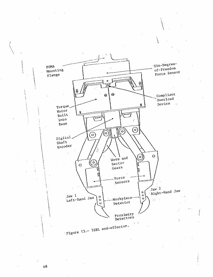
•Countingflange
figure 13.-
\ -proximity"~~ Detectors
end-effector.
•Six-Degree-Of-"Freedom?orce Sensor
~ OverloadDevice
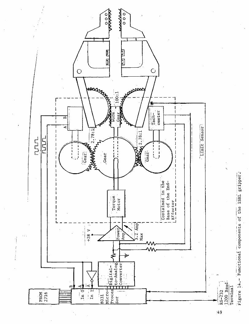
•pq
S ^>.0 r-l
P=5 r~FL, CNI
1
11
iHi ctf
4-1'-H
• • 1 ooM. - 'p
— f»•
i
^ j
->
to-A
nal
og
iC
on
ver
ter5
I I I I | I IT
I O 01I r - H M O .
CO U O '\-tS-i 'O
icno :H00
I !-i! <IJ! P.i P.I-H! (-1! 60
i f f !
•COCM OI O
Mi w1 a); co: p.
. oi a
, cd: 0: O
iii
-*iH
: 0)! 3
; a)
•49
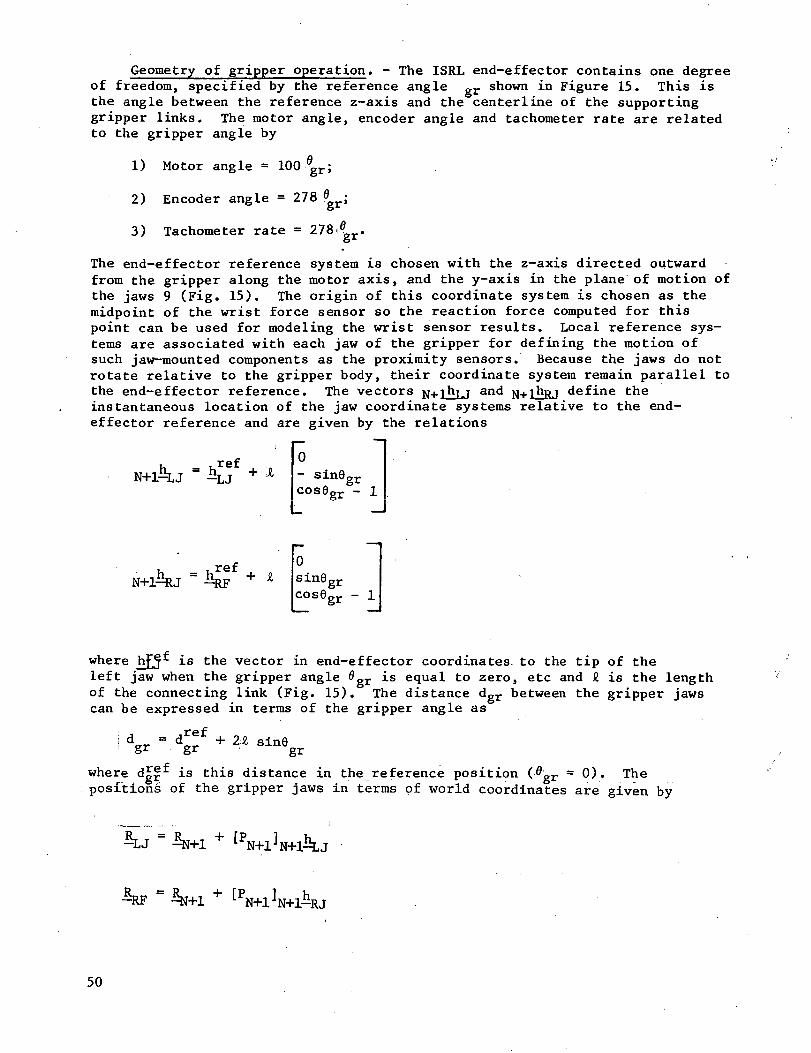
Geometry of gripper operation. - The ISRL end-effector contains one degreeof freedom, specified by the reference angle gr shown in Figure 15. This isthe angle between the reference z-axis and the centerline of the supportinggripper links. The motor angle, encoder angle and tachometer rate are relatedto the gripper angle by
1) Motor angle = 100 0gr;
2) Encoder angle = 278 ? ;
3) Tachometer rate = 278 J.
The end-effector reference system is chosen with the z-axis directed outwardfrom the gripper along the motor axis, and the y-axis in the plane of motion ofthe jaws 9 (Fig. 15). The origin of this coordinate system is chosen as themidpoint of the wrist force sensor so the reaction force computed for thispoint can be used for modeling the wrist sensor results. Local reference sys-tems are associated with each jaw of the gripper for defining the motion ofsuch jaw-mounted components as the proximity sensors. Because the jaws do notrotate relative to the gripper body, their coordinate system remain parallel tothe end-effector reference. The vectors N+lliLJ an<* N+lJiRJ define theinstantaneous location of the jaw coordinate systems relative to the end-effector reference and are given by the relations
T-af
N + j0- sin6grcose2r - 1
ref 0sin6grcos6gr -
where hffi* is the vector in end-effector coordinates, to the tip of theleft jaw when the gripper angle 6 r is equal to zero, etc and C is the lengthof the connecting link (Fig. 15). The distance dgr between the gripper jawscan be expressed in terms of the gripper angle as
gr
where d£§* is this distance in the reference position ( gr = 0). The« * • - — • * - f t * • _ _ . . .
positions of the gripper jaws in terms of world coordinates are given by
[PN+lVl-RJ
50
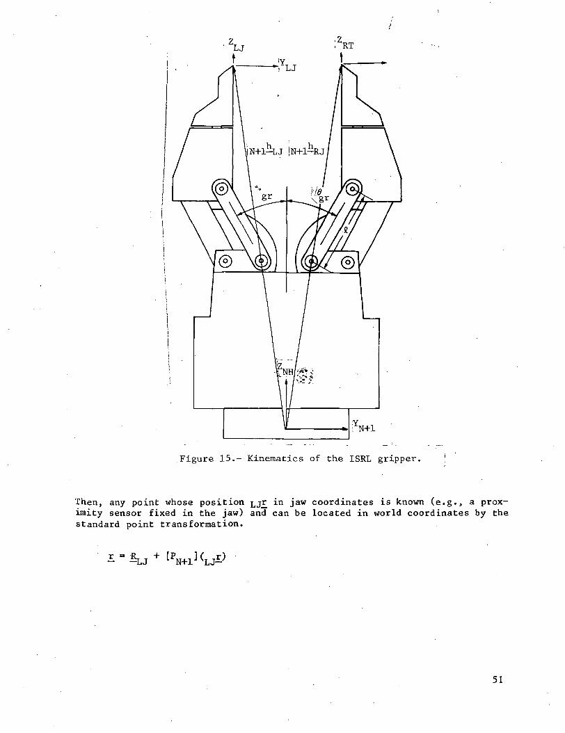
N+l
Figure 15.- Kinematics of the ISRL gripper.
Then, any point whose position LJT in jaw coordinates is known (e.g., a prox-imity sensor fixed in the jaw) and can be located in world coordinates by thestandard point transformation.
51
Gripper dynamics. - The dynamics associated with the single-degree-of-freedom gripper operation can be characterized by a second-order piecewise lin-ear system. Figure L6(a) shows a block diagram representation of this system;it includes analog rate feedback from the tachometer, viscous friction, a cou-lomb friction term and the jaw gripping force. The symbols in this diagram in-clude:
'dac
Kamp
Kemf
Ktach
Kev
Kec
output voltage from the digital-to-analog converter
s ervoamp1i f i er ga in
back emf coefficient for the gripper motor
tachometer coefficient relating tach voltage to gripper speed
effective viscous friction coefficient
effective coulomb friction coefficient
effective torque constant for the motor
motor circuit resistance
effective inertia of the gripper motor, gears, linkage and jaws
gripping force
Tp - effective torque due to gripping force
s - Laplace variable
The gripper angle ,'0gr forms the reference coordinate for most of these terms(Fig.16); for example Kev gives the torque referenced to J9gr correspondingto velocity ;6Kr' The voltage from the digital-to-analog converter is deter-mined by the control law implemented in the microprocessor controller, gripperangle feedback from the digital encoder and a reference angle supplied by auser or host computer.
52
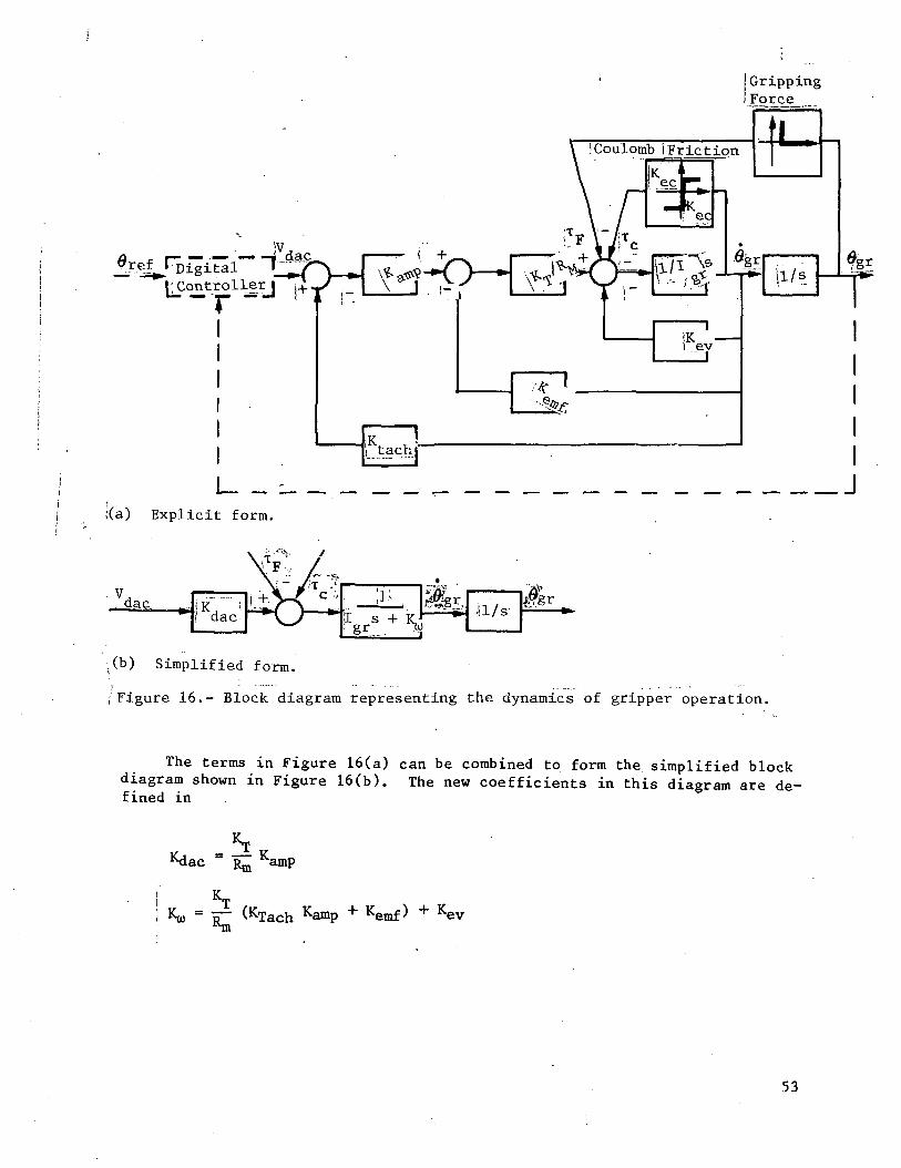
GrippingForce
I
:(b) Simplified form.
(Figure 16.- Block diagram representing the dynamics of gripper operation.
The terms in Figure 16(a) can be combined to form the simplified blockdiagram shown in Figure 16(b). The new coefficients in this diagram are de-fined in
Kamp
—Kemf > + Kev
53
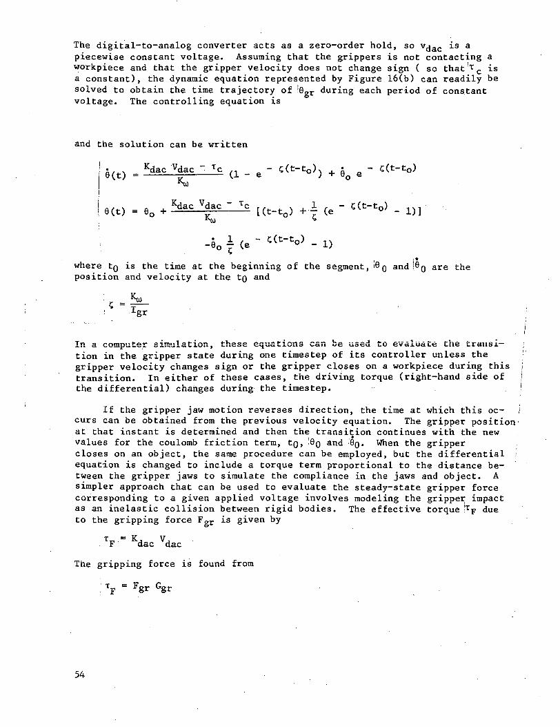
The digital-to-analog converter acts as a zero-order hold, so v(jac is apiecewise constant voltage. Assuming that the grippers is not contacting aworkpiece and that the gripper velocity does not change sign ( so that Tc isa constant), the dynamic equation represented by Figure 16(b) can readily besolved to obtain the time trajectory of '6gr during each period of constantvoltage. The controlling equation is
and the solution can be written
6(t) . 6o + dac - ?c [(t +l (e - C(t-t0) _
-e0 (a - -o - i)
where tQ is the time at the beginning of the segment, i6 Q and PQ are theposition and velocity at the to and
In a computer simulation, these equations can be used to evaluate the transi-tion in the gripper state during one timestep of its controller unless thegripper velocity changes sign or the gripper closes on a workpiece during thistransition. In either of these cases, the driving torque (right-hand side ofthe differential) changes during the timestep.
If the gripper jaw motion reverses direction, the time at which this oc-curs can be obtained from the previous velocity equation. The gripper positionat that instant is determined and then the transition continues with the newvalues for the coulomb friction term, tQ, QQ and 69. When the grippercloses on an object, the same procedure can be employed, but the differential ;equation is changed to include a torque term proportional to the distance be-tween the gripper jaws to simulate the compliance in the jaws and object. Asimpler approach that can be used to evaluate the steady-state gripper forcecorresponding to a given applied voltage involves modeling the gripper impactas an inelastic collision between rigid bodies. The effective torque !TF dueto the gripping force Fgr is given by
TF = Kdac Vdac
The gripping force is found from
; TF = Fgr Ggr
54
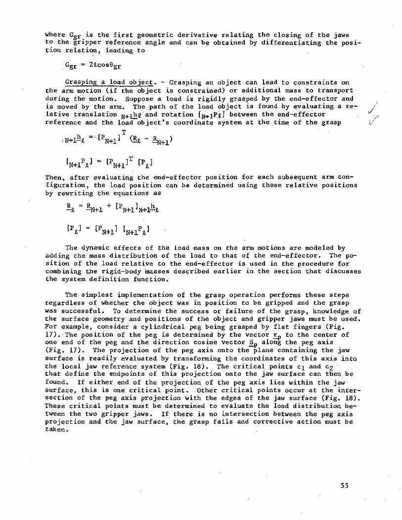
where Ggr is the first geometric derivative relating the closing of the jawsto the gripper reference angle and can be obtained by differentiating the posi-tion relation, leading to
Ggr = 2&cos0gr
Grasping a load object. - Grasping an object can lead to constraints onthe arm motion (if the object is constrained) or additional mass to transportduring the motion. Suppose a load is rigidly grasped by the end-effector andis moved by the arm. The path of the load object is found by evaluating a re- >lative translation C an<* rotation [P] between the end-effectorreference and the load object's coordinate system at the time of the grasp
Then, after evaluating the end-effector position for each subsequent arm con-figuration, the load position can be determined using these relative positionsby rewriting the equations as
The dynamic effects of the load mass on the arm motions are modeled byadding the mass distribution of the load to that of the end-effector. The po-sition of the load relative to the end-effector is used in the procedure forcombining the rigid-body ma.sses described earlier in the section that discussesthe system definition function.
The simplest implementation of the grasp operation performs these stepsregardless of whether the object was in position to be gripped and the graspwas successful. To determine the success or failure of the grasp, knowledge ofthe surface geometry and positions of the object and gripper jaws must be used.For example, consider a cylindrical peg being grasped by flat fingers (Fig.17). The position of the peg is determined by the vector jcp to the center ofone end of the peg and the direction cosine vector J3p along the peg axis(Fig. 17). The projection of the peg axis onto the plane containing the jawsurface is readily evaluated by transforming the coordinates of this axis intothe local jaw reference system (Fig. 18). The critical points c± and G£that define the endpoints of this projection onto the jaw surface can then befound. If either end of the projection of the peg axis lies within the jawsurface, this is one critical point. Other critical points occur at the inter-section of the peg axis projection with the edges of the jaw surface (Fig. 18).These critical points must be determined to evaluate the load distribution be-tween the two gripper jaws. If there is no intersection between the peg axisprojection and the jaw surface, the grasp fails and corrective action must betaken.
55
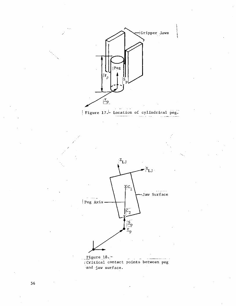
^HGripper Jaws
Figure 17.1- Location of cylindrical peg.
!Peg Axis
Jaw Surface
. Figure 18.:- _/Critical contact points between peg
•and jaw surface.
56
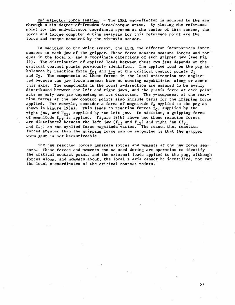
End-effector force sensing. - The ISRL end-effector is mounted to the armthrough a six-degree-of-freedom force/torque wrist. By placing the referencepoint for the end-effector coordinate system at the center of this sensor, theforce and torque computed during analysis for this reference point are theforce and torque measured by the six-axis sensor.
In addition to the wrist sensor, the ISRL end-effector incorporates forcesensors in each jaw of the gripper. These force sensors measure forces and tor-ques in the local x- and y-coordinate directions of each gripper jaw (see Fig.15). The distribution of applied loads between these two jaws depends on thecritical contact points previously identified. The applied load on the peg isbalanced by reaction force _f_£j_ and fg2 at tne critical contact points Cjand C2« The components of these forces in the local z-direction are neglec-ted because the jaw force sensors have no sensing capabilities along or aboutthis axis. The components in the local x-direction are assumed to be evenlydistributed between the left and right jaws, and the y-axis force at each pointacts on only one jaw depending on its direction. The y-component of the reac-tion forces at the jaw contact points also include terms for the gripping forceapplied. For example, consider a force of magnitude fa applied to the peg asshown in Figure 19(a). This leads to reaction forces f^, supplied by theright jaw, and F^2> supplied by the left jaw. In addition, a gripping forceof magnitude fgr is applied. Figure 19(b) shows how these reaction forcesare distributed between the left jaw (fn and f] ) and right jaw (friand fr2) as the applied force magnitude varies. The reason that reactionforces greater than the gripping force can be supported is that the gripperworm gear is not backdriveable.
The jaw reaction forces generate forces and moments at the jaw force sen-sors. These forces and moments can be used during arm operation to identifythe critical contact points and the external loads applied to the peg, althoughforces along, and moments about, the local z-axis cannot be identified, nor canthe local x-coordinates of the critical contact points.
57
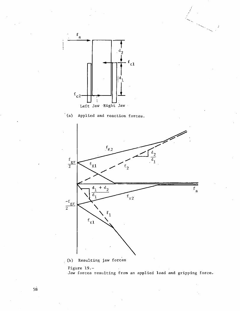
cl
c2-
id.
Left Jaw Right Jaw
(a) Applied and reaction forces.
-f
"rl
(b) Resulting jaw forces
Figure 19.-Jaw forces resulting from an applied load and gripping force.
58
POSTPROCESSING CAPABILITY
Introduction
This section describes the capabilities implemented in ROBSIM for process-ing data generated during execution of the analysis tools functions. Becauseenormous amounts of data may be generated, methods other than viewing printoutsare necessary to evaluate these data and compare different analysis runs. Thefollowing options are included in ROBSIM to accomplish this:
1) Graphics replay of simulation motion;
2) Graphics replay of simulation vs hardware motion;
3) Plots of manipulator parameters vs time.
Items I) and 2) use an Evans and Sutherland picture system to display armmotions. The replay of simulation motion displays the manipulator system mo-tions as they occurred during a requirements analysis or response simulationrun. Replay of simulation vs hardware allows the user to display the motionof actual hardware (a "real" arm) and the motion of its software model simul-taneously. The simulation model is displayed in the configuration definedduring system creation. The hardware arm is shown as a stick figure super-imposed on the simulation model. It should be noted that no calculations oranalyses are carried out during either simulation replay or simulation vs hard-ware replay other than those needed for the Evans and Sutherland display.
Manipulator parameter plots allow the user to create x-y plots of variousmanipulator parameters as functions of time. Some of the parameters availablefor plotting are joint and end-effector positions, velocities, accelerations,forces and torques. These plots may be displayed on a graphics terminal ordrawn on a pen plotter.
Simulation Replay
Replay of a manipulator system simulation displays the motions of the sys-tem exactly as they occur during a requirements analysis or response simulationrun. The system is depicted as defined during system creation/modificationwith simple cylinder components or detailed geometries. Simulation playbackmakes use of a data file, written during the analysis function, that containsmanipulator joint displacements as functions of time. These, and data definingthe system geometry, are used to locate the positions and orientations of alljoint/link pairs and load objects held by an arm with respect to the worldcoordinate system. The methods used to find these positions and orientationswere described in the System Definition and Analysis Capabilities sections.
59
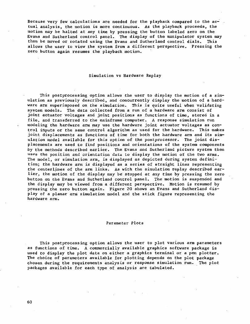
Because very few calculations are needed for the playback compared to the ac-tual analysis, the motion is more continuous. As the playback proceeds, themotion may be halted at any time by pressing the button labeled zero on theEvans and Sutherland control panel. The display of the manipulator system maythen be moved or rotated using the Evans and Sutherland control dials. Thisallows the user to view the system from a different perspective. Pressing thezero button again resumes the playback motion.
Simulation vs Hardware Replay
This postprocessing option allows the user to display the motion of a sim-ulation as previously described, and concurrently display the motion of a hard-ware arm superimposed on the simulation. This is quite useful when validatingsystem models. The data collected from a run of a hardware arm consist ofjoint actuator voltages and joint positions as functions of time, stored in afile, and transferred to the mainframe computer. A response simulation runmodeling the hardware arm may use the hardware joint actuator voltages as con-trol inputs or the same control algorithm as used for the hardware. This makesjoint displacements as functions of time for both the hardware arm and its sim-ulation model available for this option of the postprocessor. The joint dis-placements are used to find positions and orientations of the system componentsby the methods described earlier. The Evans and Sutherland picture system thenuses the position and orientation data to display the motion of the two arms.The model, or simulation arm, is displayed as depicted during system defini-tion; the hardware arm is displayed as a series of straight lines representingthe centerlines of the arm links. As with the simulation replay described ear-lier, the motion of the display may be stopped at any time by pressing the zerobutton on the Evans and Sutherland control panel. The motion is suspended andthe display may be viewed from a different perspective. Motion is resumed bypressing the zero button again. Figure 20 shows an Evans and Sutherland dis-play of a planar arm simulation model and the stick figure representing thehardware arm.
Parameter Plots
This postprocessing option allows the user to plot various arm parametersas functions of time. A commercially available graphics software package isused to display the plot data on either a graphics terminal or a pen plotter.The choice of parameters available for plotting depends on the plot packagechosen during the requirements analysis or response simulation run. The plotpackages available for each type of analysis are tabulated.
60
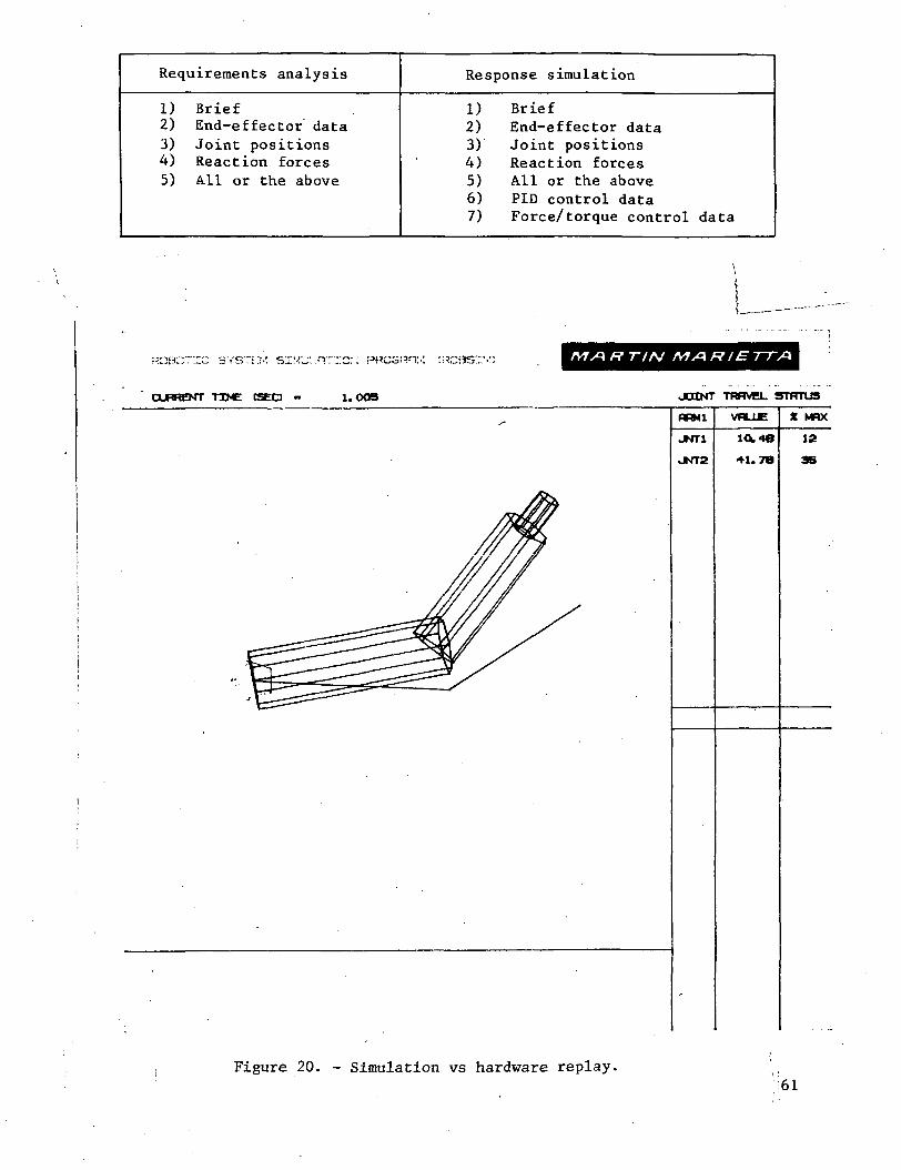
Requirements analysis Response simulation
1) Brief2) End-effector data3) Joint positions4) Reaction forces5) All or the above
1) Brief2) End-effector data3) Joint positions4) Reaction forces5) All or the above6) PID control data7) Force/ torque control data
/V7X1 Ft TIN MA HIE TTA
TIME C5ECJ " 1.009 JOINT TRRVEL STRTUS
RRM1
JMT1
JNT2
VBLJLE
10.4e•41.78
t MRX
12
Figure 20. - Simulation vs hardware replay.
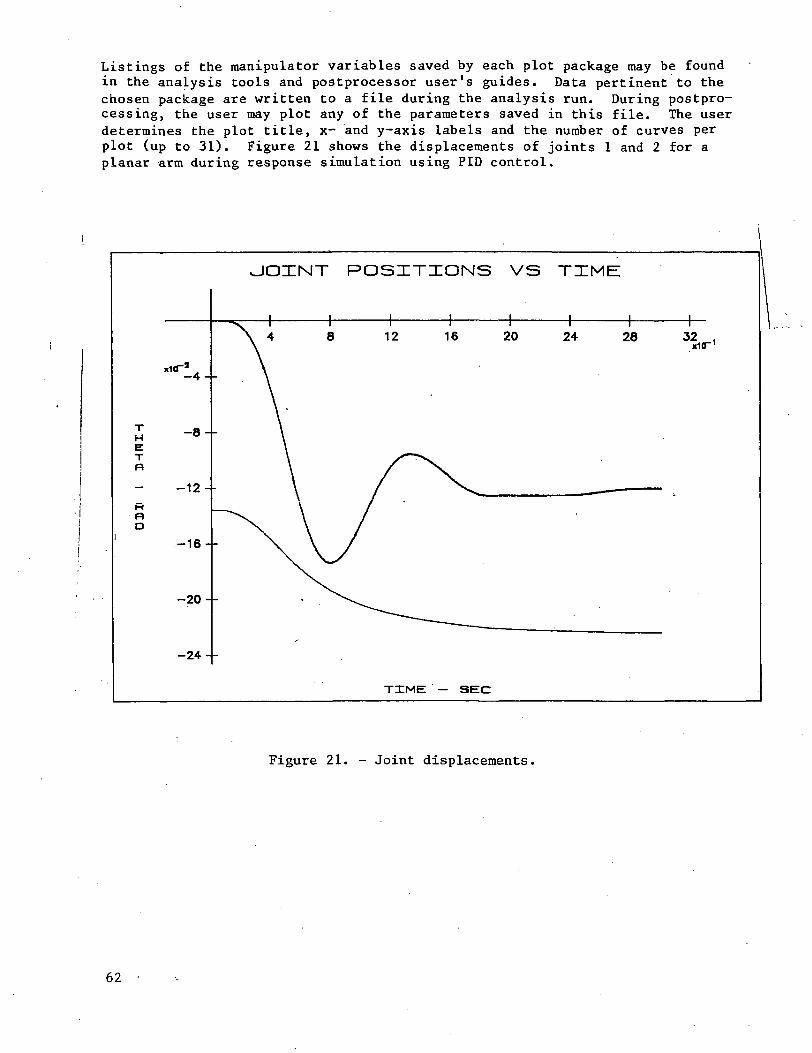
Listings of the manipulator variables saved by each plot package may be foundin the analysis tools and postprocessor user's guides. Data pertinent to thechosen package are written to a file during the analysis run. During postpro-cessing, the user may plot any of the parameters saved in this file. The userdetermines the plot title, x- and y-axis labels and the number of curves perplot (up to 31). Figure 21 shows the displacements of joints 1 and 2 for aplanar arm during response simulation using PID control.
JOINT POSITIONS VS TIME
HET1=1
R1=1O
-12--
-16--
-20--
-24--
TIME — SEC
Figure 21. - Joint displacements.
62
MANIPULATOR CONTROL
As the number of manipulators used in various applications increases, thedemands placed on control systems and sensor performance also increase. Theareas in which the demands occur are accuracy (implying repeatability), speed,and uniformity of performance over a range of loading conditions. Efficiencyof operation—implying the use of optimization techniques—is also becoming im-portant, especially with regard to long-duration space missions and high-volumeindustrial operations. This section focuses on the different families of al-gorithms used for manipulator control.
In the Manipulator Description section the basic manipulator problem isdefined in terms of fundamental elements—dyanmics, reference frame transforma-tions, and performance requirements. The Control Algorithms section describesseveral conventional position control approaches. The control algorithms dis-cussed are:
1) Linear discrete with feedforward nonlinear compensation;
2) Resolved acceleration;
3) Resolved motion force.
The Adaptive Control section discussion includes both linear adaptive con-trol and nonlinear adaptive control. Simulation results are presented for bothcases•
The Force/Torque Control section introduces the subject of control invol-ving both positional and force constraints. Two approaches, hybrid control andactive stiffness control, are analyzed in detail and simulation results pre-sented.
Manipulator Description
A full description of the plant to be controlled is required as the firststep in any control analysis. This section describes the properties of themanipulator important to control system synthesis:
1) Kinematics;
2) Dynamics;
3) Performance requirements.
63
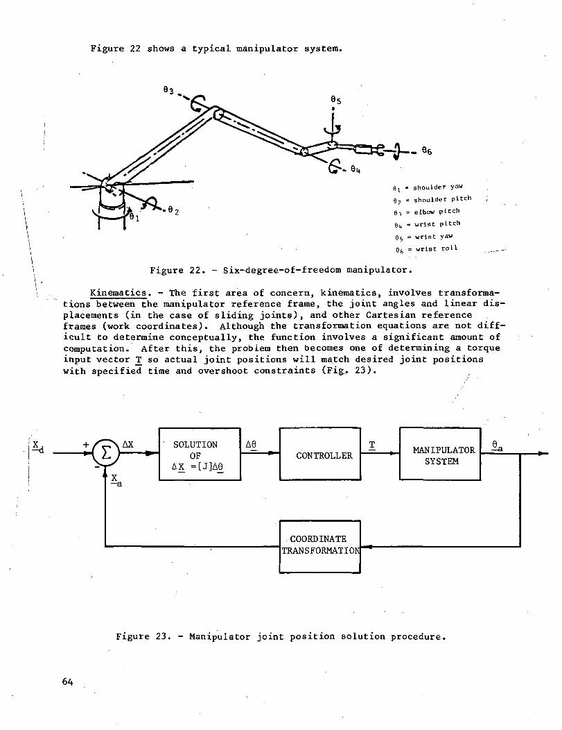
Figure 22 shows a typical manipulator system.
6-,
Bu
05
96
shoulder yaw
shoulder pitch
elbow pi tch
wrist pi tch
wrist yaw
wrist roll
Figure 22. - Six-degree-of-freedom manipulator.
Kinematics. - The first area of concern, kinematics, involves transforma-tions between the manipulator reference frame, the joint angles and linear dis-placements (in the case of sliding joints), and other Cartesian referenceframes (work coordinates). Although the transformation equations are not diff-icult to determine conceptually, the function involves a significant amount ofcomputation. After this, the problem then becomes one of determining a torqueinput vector T_ so actual joint positions will match desired joint positionswith specified time and overshoot constraints (Fig. 23).
SOLUTIONOF
AX =[J]A6
A6CONTROLLER
MANIPULATORSYSTEM
COORDINATETRANSFORMATION
Figure 23. - Manipulator joint position solution procedure.
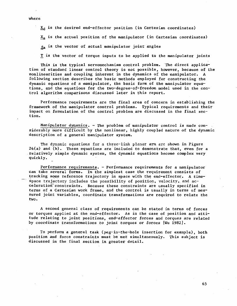
where
X^ is the desired end-effector position (in Cartesian coordinates)
Xg is the actual position of the manipulator (in Cartesian coordinates)
0a is the vector of actual manipulator joint angles
T_ is the vector of torque inputs to be applied to the manipulator joints
This is the typical servomechanism control problem. The direct applica-tion of standard linear control theory is not possible, however, because of thenonlinearities and coupling inherent in the dynamics of the manipulator. Afollowing section describes the basic methods employed for constructing thedynamic equations of a manipulator, the basic form of the manipulator equa-tions, and the equations for the two-degree-of-freedom model used in the con-trol algorithm comparisons discussed later in this report.
Performance requirements are the final area of concern in establishing theframework of the manipulator control problems. Typical requirements and theirimpact on formulation of the control problem are discussed in the final sec-tion.
Manipulator dynamics. - The problem of manipulator control is made con-siderably more difficult by the nonlinear, highly coupled nature of the dynamicdescription of a general manipulator system.
The dynamic equations for a three-link planar ana are shown in Figure24(a) and (b). These equations are included to demonstrate that, even for arelatively simple dynamic system, the dynamic equations become complex veryquickly.
Performance requirements. - Performance requirements for a manipulatorcan take several forms. In the simplest case the requirement consists oftracking some reference trajectory in space with the end-effector. A time-space trajectory includes the possibility of position, velocity, and ac-celeration" constraints. Because these constraints are usually specified interms of a Cartesian work frame, and the control is usually in terms of mea-sured joint variables, coordinate transformations are required to relate thetwo.
A second general class of requirements can be stated in terms of forcesor torques applied at the end-effector. As in the case of position and atti-tude relating to joint positions, end-effector forces and torques are relatedby coordinate transformations to joint torques or forces [Wu 1982],
To perform a general task (peg-in-the-hole insertion for example), bothposition and force constraints must be met simultaneously. This subject isdiscussed in the final section in greater detail.
65
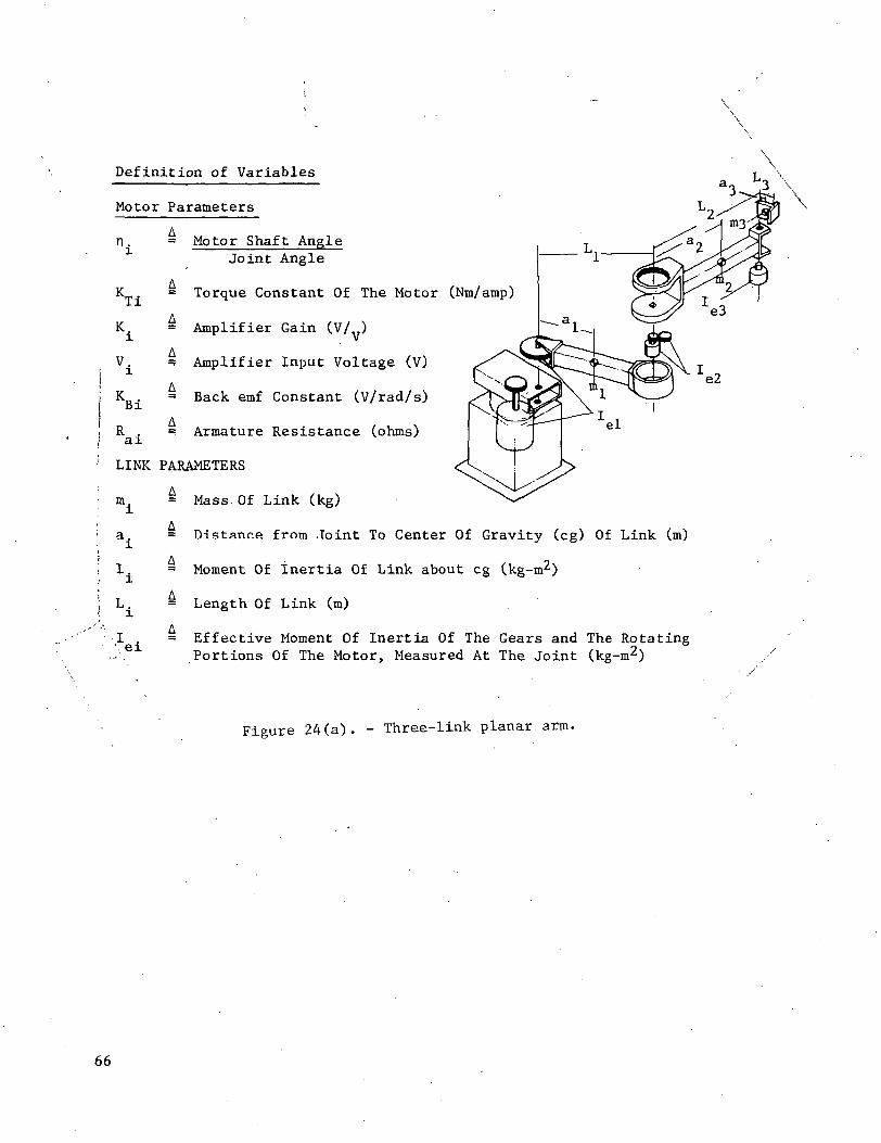
Definition of Variables
Motor Parameters
"i
KTi
K.
V.1
Bi
Motor Shaft AngleJoint Angle
Torque Constant Of The Motor (Nm/amp)
= Amplifier Gain (V/v>
=? Amplifier Input Voltage (V)
= Back emf Constant (V/rad/s)
= Armature Resistance (ohms)
K
R .ai
LINK PARAMETERS
m.i
a.i
I
e2
ei
= Mass.Of Link (kg)
= Distance from Joint To Center Of Gravity (eg) Of Link (m)
= Moment Of inertia Of Link about eg (kg-m2)
= Length Of Link (m)
= Effective Moment Of Inertia Of The Gears and The RotatingPortions Of The Motor, Measured At The Joint (kg-m2)
Figure 24(a). - Three-link planar arm.
66

"Page missing from available version"
A^fr
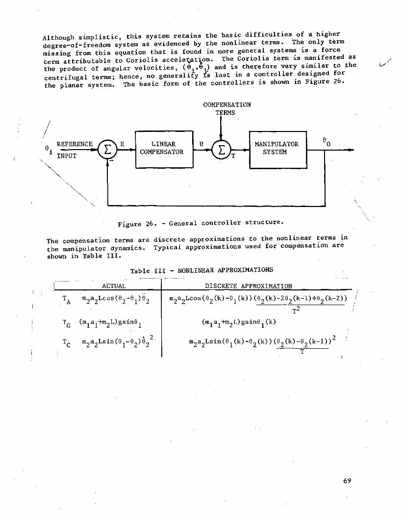
Although simplistic, this system retains the basic difficulties of a higherdegree-of-freedom system as evidenced by the nonlinear terms. The only termmissing from this equation that is found in more general systems is a forceterm attributable to Coriolis acceleration. The Coriolis term is manifested asthe product of angular velocities, (-.8 ,8 ) and is therefore very similar to thecentrifugal terms; hence, no generality is lost in a controller designed forthe planar system. The basic form of the controllers is shown in Figure 26.
COMPENSATIONTERMS
REFERENCED ~1 INPUT *•
LINEARCOMPENSATOR
MANIPULATORSYSTEM
Figure 26. - General controller structure.
The compensation terms are discrete approximations to the nonlinear terms inthe manipulator dynamics. Typical approximations used for compensation are
shown in Table III.
Table III - NONLINEAR APPROXIMATIONS
ACTUAL DISCRETE APPROXIMATION
2.
m9a Lcos(69(k)-01(k))(eo(k)-269(k-l)+eo(k-2))^- £. £- 1 Z _ £. __ _Z _
L) gsinO (k)
m2a2Lsin(81(k)-e2(k))(e2(k)-02(k-l))'
T
69
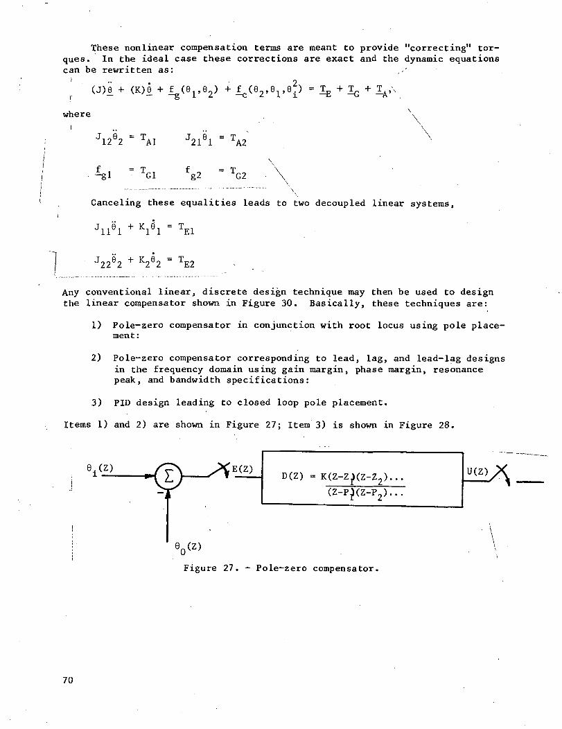
These nonlinear compensation terms are meant to provide "correcting" tor-ques. In the ideal case these corrections are exact and the dynamic equationscan be rewritten as: .,• •
(j)e.
where
J1282 - TA1 J2161 " TA2
= T f = TGl g2 TG2
Canceling these equalities leads to two decoupled linear systems,
J1161 + Vl - TE1
J2262 + K262 ~ TE2
Any conventional linear, discrete design technique may then be used to designthe linear compensator shown in Figure 30. Basically, these techniques are:
1) Pole-zero compensator in conjunction with root locus using pole place-ment:
2) Pole-zero compensator corresponding to lead, lag, and lead-lag designsin the frequency domain using gain margin, phase margin, resonancepeak, and bandwidth specifications:
3) PID design leading to closed loop pole placement.
Items 1) and 2) are shown in Figure 27; Item 3) is shown in Figure 28.
D(Z) = K(Z-Z£(Z-Z2) ,
(z-pJ(z-P2).
e0(z)
Figure 27. - Pole-zero compensator.
70
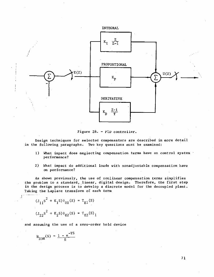
E(Z)
INTEGRAL
KI Z-l
PROPORTIONAL
DERIVATIVE
Figure 28. - PJ.D controller.
Design techniques for selected compensators are described in more detailin the following paragraphs. Two key questions must be examined:
1) What impact does neglecting compensation terms have on control systemperformance?
2) What impact do additional loads with nonadjustable compensation haveon performance?
As shown previously, the use of nonlinear compensation terms simplifiesthe problem to a standard, linear, digital design. Therefore, the first stepin the design process is to develop a discrete model for the decoupled plant.Taking the Laplace transform of each term
K1S)6n1(S) =
(J22S +K 2 S)6 0 2 (S ) = TE
and assuming the use of a zero-order hold device
H (S) = 1 ~H V '
-TS
71
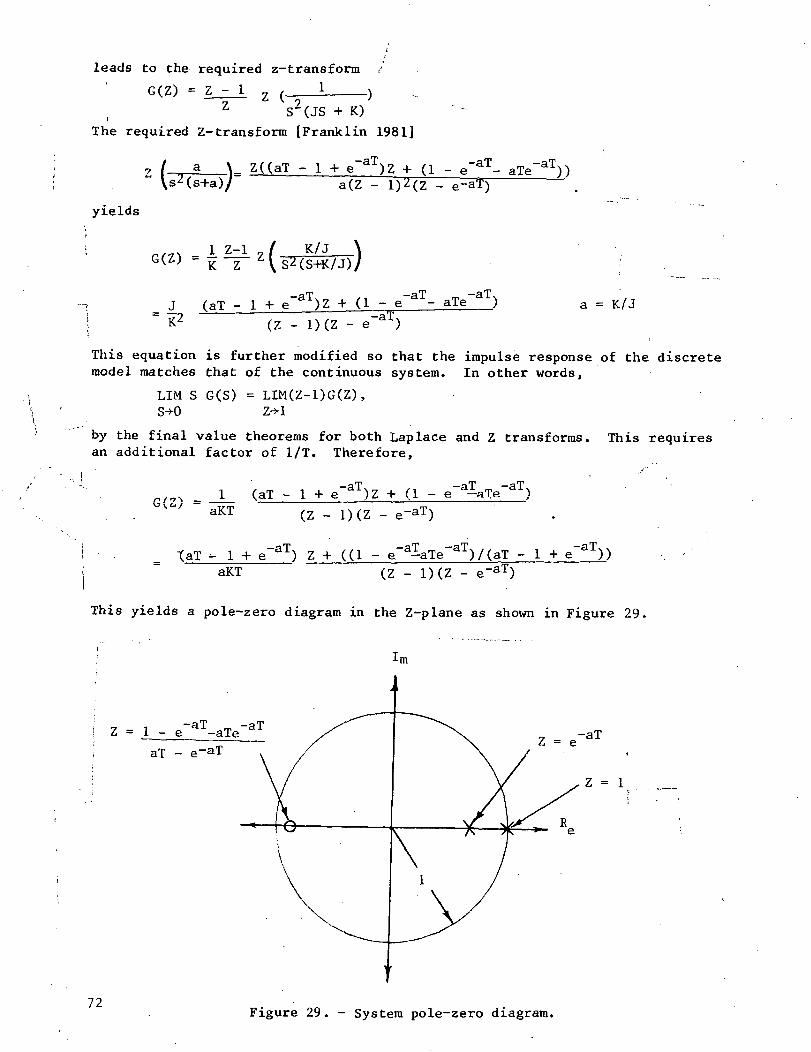
leads to the required z-transform
G(Z) = Z - 1 - !Z S2(JS + K)
The required Z-transform [Franklin 1981]
•7 / . . - a \" \s2(s+a)/
= Z((aT - 1 + e )Z + (1 -a(Z -
e"aT- aTe-aT))
yields
K Z
K/J
J (aT -= K2
- aTe a = K/J
(Z - 1)(Z - e
This equation is further modified so that the impulse response of the discretemodel matches that of the continuous system. In other words,
LIM S G(S) = LIM(Z-1)G(Z),S-K) Z->1
by the final value theorems for both Laplace and Z transforms. This requiresan additional factor of 1/T. Therefore,
aKT(aT - 1 + e aT)Z + (1 - e
aT)
(Z - 1)(Z -
-(aT - 1 + e"aT) Z + ((1 - e a-aTe aT)/(aT - 1 + e'aKT (Z - 1)(Z - e~aT)
This yields a pole-zero diagram in the Z-plane as shown in Figure 29.
Lm
72
Z = e! Z = 1 - e -aTe -aT
Z = 1
Figure 29. - System pole-zero diagram.
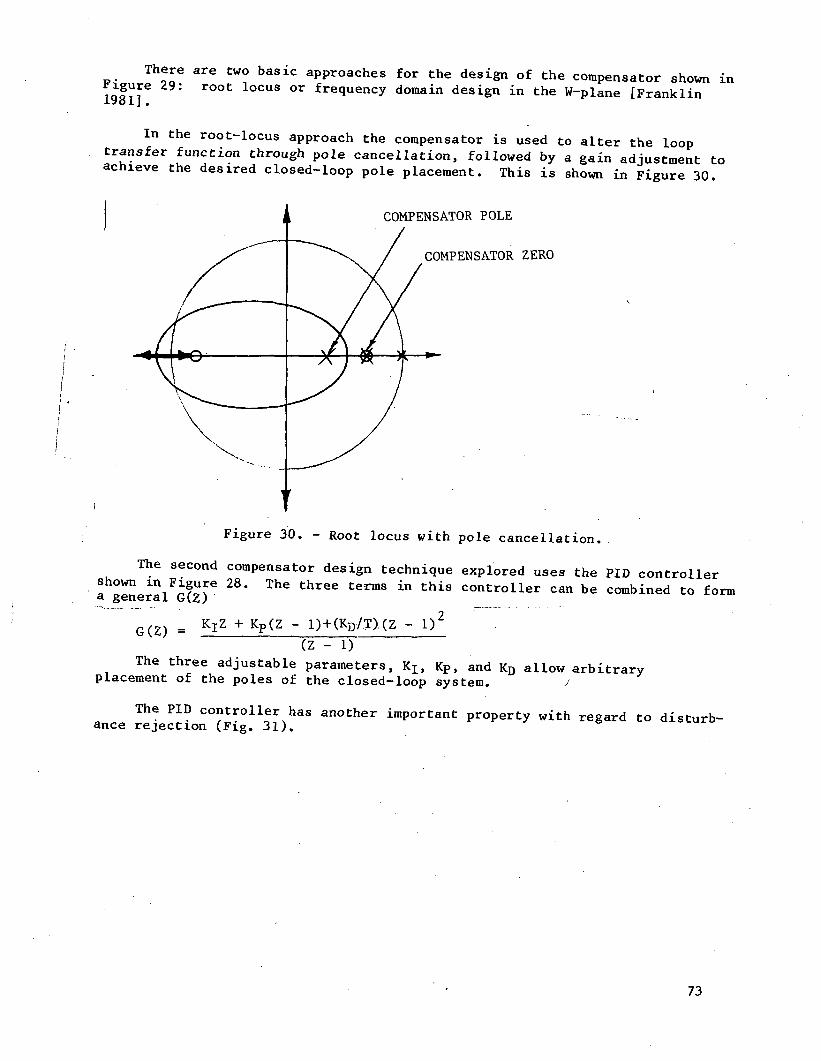
There are two basic approaches for the design of the compensator shownr°0t 10CUS °r fre<luency domain design in the W-plane [Franklin
in
In the root-locus approach the compensator is used to alter the looptransfer function through pole cancellation, followed by a gain adjustment toachieve the desired closed-loop pole placement. This is shown in Figure 30.
COMPENSATOR POLE
COMPENSATOR ZERO
Figure 30. - Root locus with pole cancellation.
The second compensator design technique explored uses the PID controller
**' ^^ ^^ ™ "^ C°ntroller can be combined to form
G(Z) = KIZ + Kp(Z - 1) + (KD/,T).(Z - I)2
(Z - 1)
The three adjustable parameters, KL, KP, and KD allow arbitraryplacement of the poles of the closed-loop system. j
The PID controller has another important property with regard to disturb-ance rejection (Fig. 31).
73
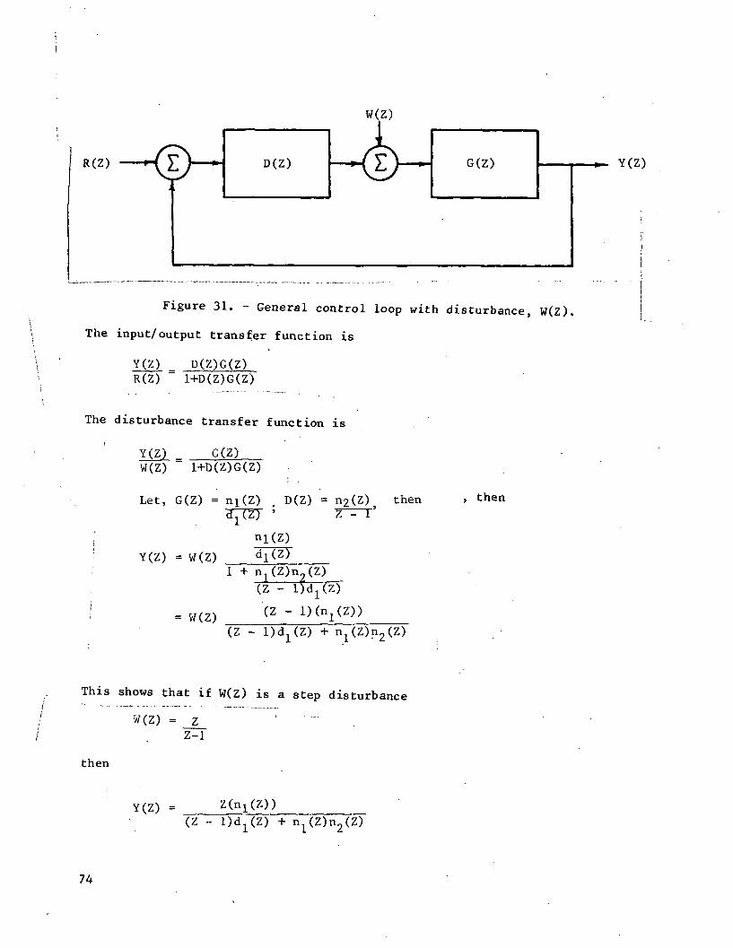
W(Z)
R(Z) D(Z) G(Z) Y(Z)
Figure 31. - General control loop with disturbance, W(Z)
The input/output transfer function is
Y(Z) = D(Z)G(Z)R(Z) 1+D(Z)G(Z)
The disturbance transfer function is
Y(Z) = G(Z)W(Z) 1+D(Z)G(Z)
Let, G(Z) = ni(Z) . D(Z) = n
1ni(Z)
Y(Z) = W(Z) dl(z)
= W(Z)
then » then
1 + ni(Z)n2(Z
(Z - l)dj
(Z -
_
(Z)
(Z -
This shows that if W(Z) is a step disturbance
W(Z) = ZZ-l
then
Y(Z) = Z(ni(Z))(Z - + ni(Z)n2(Z)
74
If the denominator has roots inside the unit circle, the steady-state re-sponse to a step, disturbance is zero; i.e., there is no steady-state "offset."This is attributable to the pure integrator in the controller. In contrast,assume (Z-l) is replaced by some general d£(z) in the disturbance transferfunction. Then for a step disturbance
Y(Z) = Z d2(Z)n1(Z)Z-l d1(Z)d2(Z) +"n1(Z)n2(Z)
/
The steady—state contains a step component
Y (Z) = LIM Zd2(Z)ni(Z)step Z+l d1(Z)d2(Z) + n
This implies that there will be a steady-state error to a step disturb-ance. The physical interpretation of these results is straightforward. Atequilibrium, in the non-PID case, a non-zero error is required to provide thetorque necessary to maintain equilibrium. In the PID case, the error can bezero while the output from the integrator provides the torque to counter thedisturbance. From the standpoint of a manipulator system this is an interest-ing property because gravity disturbances are essentially step disturbancesaround a given operating region.
Resolved acceleration control (RAG). - The RAG is a method of positioncontrol of a manipulator. The algorithm uses the position and orientation,the velocity, and the acceleration of the hand (or end-effector). The desiredposition and orientation, velocity, and acceleration of the hand are specifiedat each time step, and the control algorithm determines the joint positions,velocities, and accelerations required to satisfy the specified conditions.Finally, the input forces and torques to be applied to the joints are calcu-lated using the "inverse problem" technique [Luh 1980a].
One advantage of the RAG method is that the forces and torques are not ob-tained by the dynamics equations; rather they are calculated as a function ofthe desired and actual joint positions, velocities, and accelerations, usingthe Newton-Euler formulation of the manipulator equations. The method succes-sively transforms the velocities and accelerations from the base to the hand,using moving coordinate system relationships. The input forces and torques arecomputed for each link (working back from the hand to the base). This schemeallows much faster computation than the conventional technique based on theLagragian formulation of the dynamics [Luh 1980b] .
Resolved motion force control (RMFC). - RMFC is a position control methoddeveloped for robot manipulators [Wu 1982]. Rather than controlling the jointpositions and torques (as do classical control techniques), RMFC controls Car-tesian positions and forces. This method has the advantage of automaticallycompensating for the changing configuration of the manipulator, gravity forces,and the internal friction of the manipulator. Another advantage of RMFC isthat the control method can be extended to more than six degrees of freedomwithout increasing the computational complexity.
75
To effect control of a position manipulator, it is usually desired todrive it to follow a given trajectory. Paul's method of defining a manipula-tor's position and orientation, the relationship between Cartesian forces andmanipulator joint torques, the specification of a manipulator's position tra-jectory, and the RMFC algorithm are discussed below.
The position and orientation of an n-link manipulator can be described bya 4x4 transformation matrix
n ox xax Px
n,,, n,where P = (px pv pz) is the position and nx, uy, nz, ux,ay and az are the direction cosines defining the manipulator's orientation.
Jz »
The matrix Tn is the product of all n transformation matrices, A£,i = 1 to n, describing the position and orientation of link i relative to link
Tn = A2 ... An
The linear and angular velocities of the terminal link are a function ofthe Jacobian and the joint rates
x = IJ]£
where x =fv~|= l£I w|= an
= linear velocityangular velocity
The terminal link static forces Fn =n *[f t<i ... fn-i f
Fy Fz and tne
are relatedstatic joint torques
Ft = [JjTFa
where
[j]" is the transpose of the Jacobian; the differential change in posi-tion and orientation of Tn as a function of all n joint angles
fj, ... fn are the joint torques; FX, F , and FZ are theCartesian forces at the end-effector
Mx, My, and Mz are the moments at the end-effector
A time-based position trajectory can be defined as:i
Tn(t+ t) =1
76
1
w z ( t )
-wy(t)
0
-wz(t)
1
wx(t)
0
wy(t)
-wx(t)
1
0
vx(t)
vy(t)
v z( t)
1
At
where v(t) is the linear velocity and w(t) is the angular velocity Tn(t),v(t), and w(t) must be continuous.
The basic idea of RMFC is to calculate the joint torques required to con-trol the Cartesian motion of the manipulator. The method is based on the rela-tionship between the joint torques and the terminal link forces. The controlis divided into two parts. The first part deals with position control of theterminal link. The second part of resolved motion force control calculates thejoint torques required to obtain the desired terminal link forces and momentsthat were determined in the first part.
For the first part of the control it is assumed that all links except theterminal link and the load are massless. Also, the center of mass of the loadis located at the origin of the terminal link coordinate system, and the coor-dinate axes of the load are aligned with the terminal link axes. Because themanipulator's links are not massless, the second part of the RMFC scheme com-pensates for these errors-using a method called force convergent control. Thetechnique uses the Robbins Monro stochastic approximation method to determinethe joint torques required to produce the desired Cartesian forces and momentsof the center of mass of the load.
The desired position and orientation can be expressed in the form of atransformation matrix Tn<j. The actual position and orientation Tna isdetermined according to equation for Tn above. The Cartesian position andorientation error
Xe - Xd - Xa - [dx
can be written as
x "y rzj
nd na
1
-6
-62
l
6
y
X
1
0
The differential transformation matrix is obtained as follows. The trans-formation matrices Tx, Ty, and Tz defining a rotation about the x, y and zaxes, respectively are given by
77
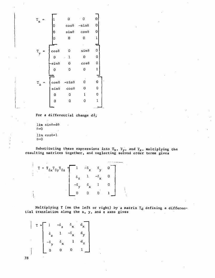
T =
T =
T =
1
0
0
0
-^= — -
cosG
0
-sine
0
cos6
sinO
0
0
0
cos6
sin9
0
0
1
0
0
-sin9
cos6
0
0
0
-sine
cose0
sine
0
cos6
0
0
0
1
0
0
0
0
1
0
0
0
1
0
0
0
1
For a differential change dOj
lim sin6=d60-K)
lim cos6=l
Substituting these expressions into Tx, Ty, and Tz , multiplying theresulting matrices together, and neglecting second order terms gives
T = T T T6x 6y 6z
1
6Z
-6y0
-6z
1
6X
0
6y-5
X
1
0
0
0 .
0
1
Multiplying T (on the left or right) by a matrix Ta defining a differen-tial translation along the x, y, and z axes gives
1
6Z
-6
78
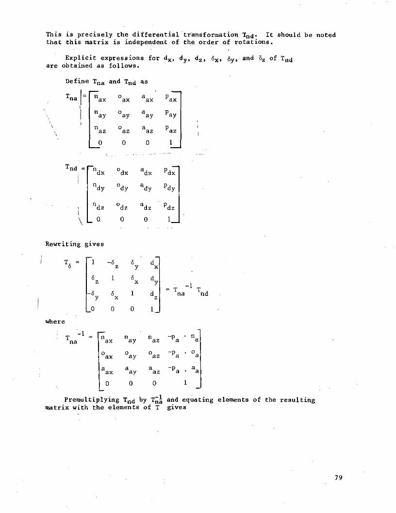
This is precisely the differential transformation Tnd« It should be notedthat this matrix is independent of the order of rotations.
Explicit expressions for dx, dy, dz, 6X, 6y» and 6Z of Tn<iare obtained as follows.
Define Tna and Tn(j as
T =•na
i
Tnd =f1
ti
\
nax
nay
naz
0
~~n !dx
n,dy
njdz
_ 0
0ax
oay
oaz
0
°dx
°dy
°dz
0
aax
aay
aaz
0
adx
ady
adz
0
Pax
ay
paz
1
Pdx~
pdy
Pdz
1_
Rewriting gives
where
na
1 -6z
6 1z
-6 6y x_0 0
= nax
°ax
aax
0
6y6X
1
0
nay
°ay
aay
0
dX
dydz
1_
= T l T .,na nd
naz -pa • %
°az -pa ' °a
a -p aaz *a- • a
0 1
Premultiplying Tn<j by T^ and equating elements of the resultingmatrix with the elements of T gives
79
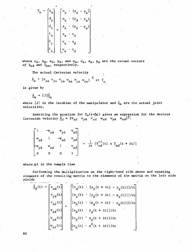
X =e
Xa • o ,a d
n • a,a d
o • n,a d
where nd, od, ad, pd, and na, oa, aa, pa are the column vectorsof Tnd and Tna, respectively.
The actual Cartesian velocity(Tl
X = TV v V w w w 1 at- T. -a L xa ys za xa ya za-1 at n
is given by
where [J] is the Jacobian of the manipulator and qa are the actual jointvelocities.
Rewriting the equation for Tn(t+At) gives an expression for the desiredCartesian velocity Xd = [Vxd vyd vzcl wxci x-7yd wz<i]
T:
~1
wzd
-w ,yd
0
-w ,zd
1
w jxd
0
wyd
-w ,xd
1
0
Vxd
vydVzd
1
*Tnd(t+At)]
where At is the sample time
Performing the multiplication on the right-hand side above and equatingelements of the resulting matrix to the elements of the matrix on the left sideyields
lnd(t) • [pd(t + At) - pd(t)]]/At
[od(t) • [pd(t + At) - pd(t)]]/At
[ad(t) • [pd(t + At) - pd(t)]]/At
[a.(t) • o,(t + At)]/At
Vyd(t)
Vzd(t>
[nd(t) ad(t + At)] /At
[od(t) • n(t + At)] /At
80
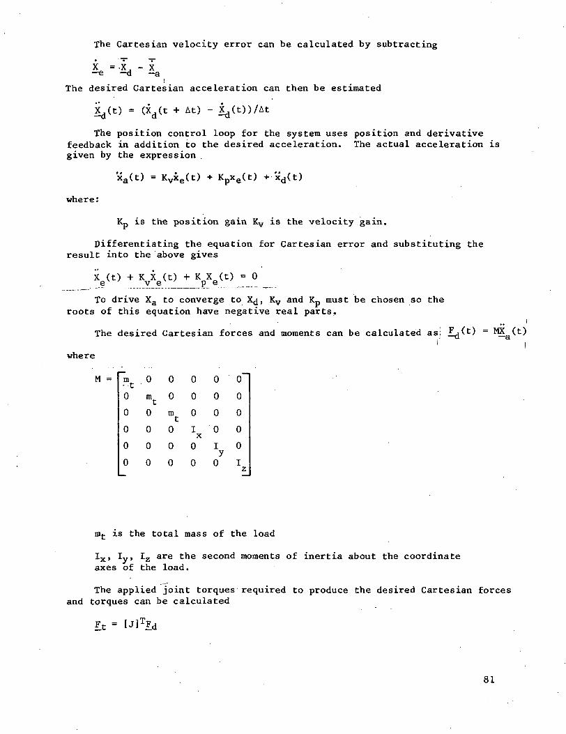
The Cartesian velocity error can be calculated by subtracting
X = -X, - X-e -=d —a
iThe desired Cartesian acceleration can then be estimated
(t) = (Xd(t + At) - Xd(t))/At
The position control loop for the system uses position and derivativefeedback in addition to the desired acceleration. The actual acceleration isgiven by the expression
where:
xa(t) = Kvxe(t) + Kpxe(t) + xd(t)
is the position gain Kv is the velocity gain.
Differentiating the equation for Cartesian error and substituting theresult into the above gives
To drive Xa to converge to X^, Kv and Kp must be chosen so theroots of this equation have negative real parts.
The desired Cartesian forces and moments can be calculated as
where
M = m• t0
0
0
0
0
0
mt
0
0
0
0
0
0
mt
0
0
0
0
0
0
IX
0
0
0
0
0
0
Iy0
0
0
0
0
0
Iz
mt is the total mass of the load
Ix, Iy, Iz are the second moments of inertia about the coordinateaxes of the load.
The applied joint torques required to produce the desired Cartesian forcesand torques can be calculated
It =
81
When the mass of the terminal link and the load approaches the mass of theremaining portion of the manipulator, the control algorithm will not convergeto the desired Cartesian forces and torques. Force convergent control compen-sates for this error.
Force convergent control uses Robbins-Monro stochastic approximation tocalculate the applied Cartesian force F^ (and the corresponding joint tor-ques) required to drive the observed Cartesian force F^ to converge to thedesired Cartesian force F j.
The Robbins-Monro method, which finds the root of a regression function,can be summarized as follows. Let be the parameter vector to be estimatedand the Zj^ be the observation at time K. Then the new estimate at time K+lis given by
The coefficient b^ is a sequence of positive numbers with the followingproperties
ilim bv = 0
K
The first equation ensures that the estimate will settle down in the lim-it. The second ensures that the estimate does not settle down before reachingthe root. The third ensures that the variance of the accumulated noise is fi-nite so the effect of the noise can be corrected [Fukunaga 1972] .
The manipulator is modeled as an unknown function. The input of the func-tion at each sample time is F_a, the applied force. The function's output isthe observed force F_o at the load. This can be stated as
F0 = F(Fa)
The method can be described as three basic steps. First, define an errortolerance for the force
dF = [dF1 dF2 dF3 dF4 dF5 dF6]T
This is the acceptable error between the observed Cartesian force F_o and thedesired Cartesian force Fjj.
Next, initialize the applied force F^ at t ~ 0 to the Cartesian forcecaused by the gravity force of the load. Finally, at each sample time, performthe following operations:
1) Calculate Fd using jj Ct) = MX^t)
2) Set K=0 and £3(0) = final F_a of previoussample time;
82
3) Apply the joint torques Ft = [J]TFa(K);
4) Measure the observed force F^dO;!
5) Calculate the Cartesian force errorl6F(K) = Zd ~ Z
6) Calculate
a) If |6Fi[ > dF± , i = 1, 2, . . . . 6, compensateF_a according to the following equation
b 6F(k)
where bR = 1/(K+1) for K = 0, 1, 2, ...
b) Increment K by 1,
c) Return to step 3 (apply new joint torques);
7)| If |6F±|-< dF ,i = 1, 2, . . . , 6, Fjo(K)has converged to the desired force F^. Therefore, apply the jointtorques in step 3) for the remaining portion of the sample time.
It should be noted that in the simulations documented in [Wu 1982], theabove algorithm was modified to perform a finite number of iterations, N,rather than using the force error criterion to test convergence. As N is in-creased, the accuracy of the algorithm increases. It should be noted furtherthat N cannot exceed At/h, where At is the sample time (in seconds) and h isthe time (in seconds) required to perform the operations in FCC.
83
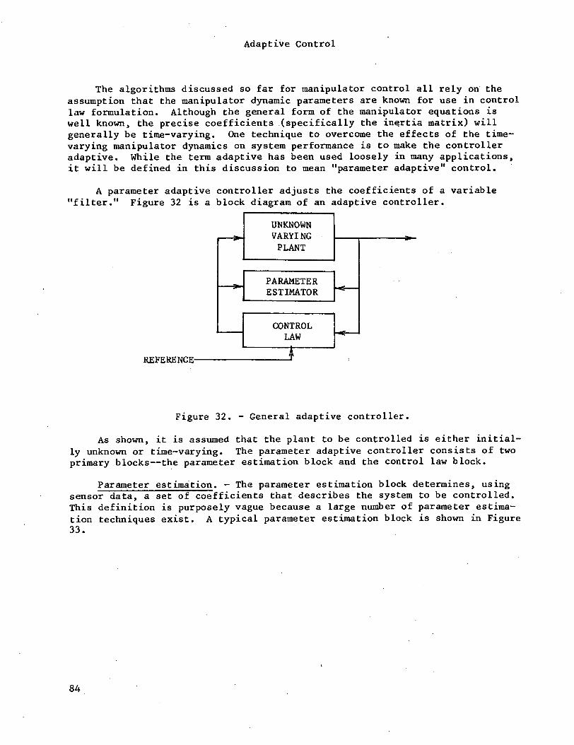
Adaptive Control
The algorithms discussed so far for manipulator control all rely on theassumption that the manipulator dynamic parameters are known for use in controllaw formulation. Although the general form of the manipulator equations iswell known, the precise coefficients (specifically the inertia matrix) willgenerally be time-varying. One technique to overcome the effects of the time-varying manipulator dynamics on system performance is to make the controlleradaptive. While the term adaptive has been used loosely in many applications,it will be defined in this discussion to mean "parameter adaptive" control.
A parameter adaptive controller adjusts the coefficients of a variable"filter." Figure 32 is a block diagram of an adaptive controller.
UNKNOWNVARYI NGPLANT
PARAMETERESTIMATOR
CONTROLLAW
REFERENCE-
Figure 32. - General adaptive controller.
As shown, it is assumed that the plant to be controlled is either initial-ly unknown or time-varying. The parameter adaptive controller consists of twoprimary blocks—the parameter estimation block and the control law block.
Parameter estimation. - The parameter estimation block determines, usingsensor data, a set of coefficients that describes the system to be controlled.This definition is purposely vague because a large number of parameter estima-tion techniques exist. A typical parameter estimation block is shown in Figure33.
84
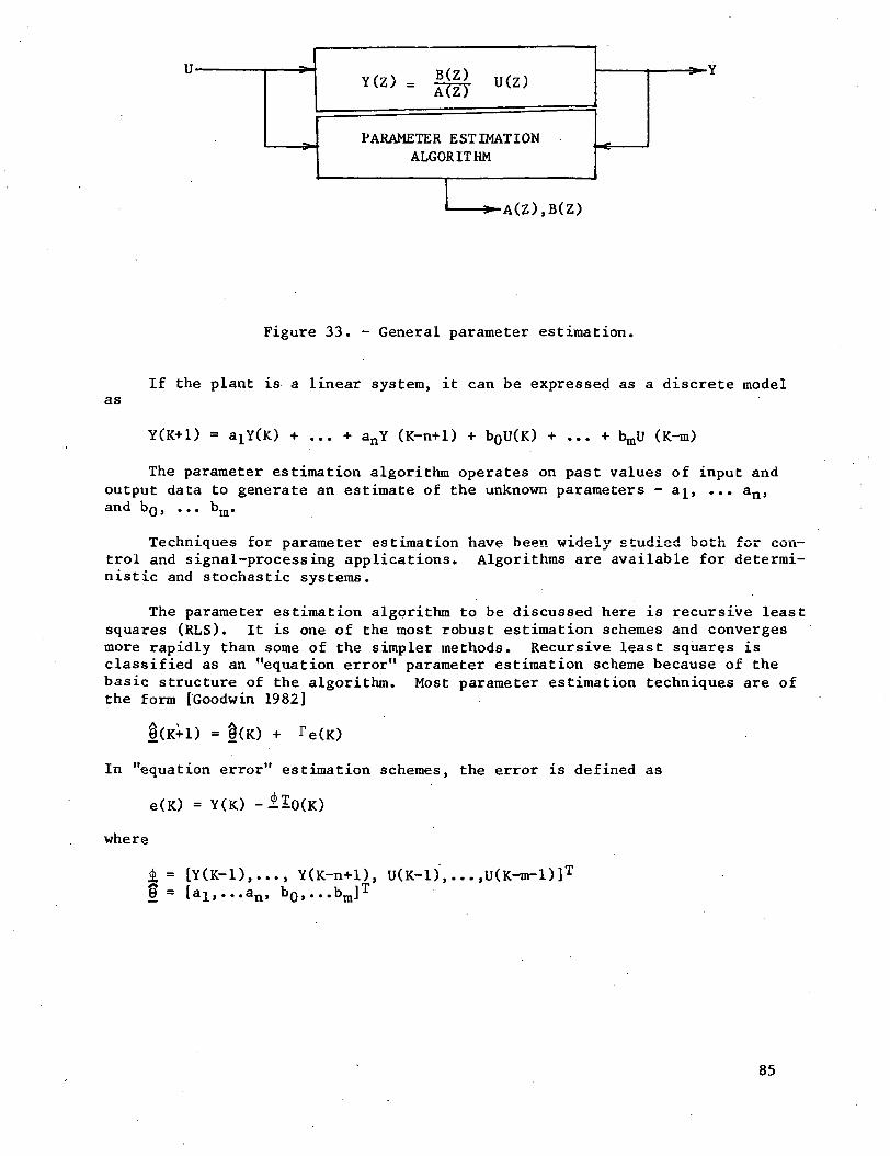
u-Y(Z) = B(Z)
A(ZU(Z)
PARAMETER ESTIMATIONALGORITHM
Figure 33. - General parameter estimation.
If the plant is a linear system, it can be expressed as a discrete modelas
= aLY(K) anY bQU(K) (K-m)
The parameter estimation algorithm operates on past values of input andoutput data to generate an estimate of the unknown parameters - aj_, ... an,and b0, ... bm.
Techniques for parameter estimation have been widely studied both for con-trol and signal-processing applications. Algorithms are available for determi-nistic and stochastic systems.
The parameter estimation algorithm to be discussed here is recursive leastsquares (RLS). It is one of the most robust estimation schemes and convergesmore rapidly than some of the simpler methods. Recursive least squares isclassified as an "equation error" parameter estimation scheme because of thebasic structure of the algorithm. Most parameter estimation techniques are ofthe form [Goodwin 1982]
In "equation error" estimation schemes, the error is defined as
e(K) = Y(K) -llo(K)
where
= [Y(K-l),..., Y(K-n+l), U(K-l), ...,U(K-m-l)]T
,...an, b0,...bm]T
85
For the true parameters, e(K) = 0. Thus the name "equation error." e(K)is a measure of how well the parameter estimates satisfy the governing equa-tion. If e(K) £ 0, the parameter estimator will continue to update the esti-mate. The ",r" term is what differentiates parameter estimation schemes. Itcan be thought of as a "gain" term for the estimation process. For the recur-sive least squares estimator, is chosen to be [Goodwin 1982] and [Franklin1981]
a(k) P(K-d-l) <}(K-d)1 — ^ - ^ • ' • • • ' ••' • -•
1 + a(K) <j)(K-d)TP(K-d-l)
and
a(K) P(K-d-l) (j)(K-d) $(K-d)TP(K-d-l)P(K-d) = P(K-d-l)
+ a(K) <f)(K-d)TP(K-d-l)
To start the RLS algorithm,
P( -d-1) = £0I
where e » 1 and
I is the identity matrix
0 <a(K) < 2f(0) = [0,..,0,1,0,...0]
where the "1" corresponds to the parameter bg.
If a good "first guess" of the parameters is available, it can be used forj|(0). The estimate of the coefficient bg should not be initialized to zerobecause this results in division of 0.
The coefficient a(K) is usually chosen to be unity; however, in caseswhere <J>(K-d)T P(K-d-l) >(K-d) (in the denominator of T ) is close to minus 1,a(K) should be chosen to avoid division by a number close to zero.
Once an estimate of the parameters has been obtained, it is used in for-mulation of the control law. The most general control form is model-referencecontrol. In this case the controller functions to make the closed-loop systemmatch a desired transfer function (or matrix). A special case of model-reference control is "one-step ahead optimal" or minimum-variance control.These control strategies are discussed in more detail in the next section.
Linear Adaptive Control. - A linear, deterministic system is described byan auto-regressive moving average (ARMA) equation of the form
= a]Y(K) + ... + anY(K-n+l) + b0 U(K) + ... + bmU(K-m)
86
To formulate a "one step-ahead" or "deadbeat" controller, it is assumedthat the reference signal is known one step in advance. That is, Y*(K+1) mustbe known at the time K. The control law for the parameter adaptive controlleris obtained by setting Y(K+1) = Y*(K+1) and solving for U(K) [Goodwin 1983].
This yields
U(K) = _!_[ -a! Y(K) - ... - anY(K-n+l) - b]U(K-l)b0 - ... -bm U(K-m) + Y*(K+1)]
This can also be written in vector notation as
U(K) = £
where £(K) = [ -Y(K) ... -Y(K-n+l) - U(K-l),-U(K-m) Y*(K+1)]T
6(K) = pil £n bjL ^LbO ••• bO» bO ••• bO>
The vector j)(K) is referred to as the regression vector and 9(K) is theparameter vector. This is referred to as the linear controller form becausethe control law is a linear function of past Y and U values. If the a and bcoefficients are known, the control for U(K) will result in Y(K+1) = Y*(K+1).Because it is assumed, however, that the system parameters are initially un-known (or time-varying in the case of manipulator control), the a and b co-efficients must be estimated. The control law then becomes
U(K) = (K)T (K-)
where 9(K) is the vector of parameter estimates.
A,The parameter estimation algorithm used to obtain 0*(K) is RLS as explained
in the previous section.
While this form of control is appealing from the standpoint of its simpli-city and apparent tracking performance, it is impractical for implementation inan actual system. The superior performance is attained at the expense of largecontrol efforts. For practical systems this leads to saturation of controlcomponents and hence full performance is never achieved.
A more reasonable approach to the problem is to force the closed-loop sys-tem to behave as some reference model that is chosen with the limitations ofamplifiers and actuators in mind. (Strictly speaking, the one-step-ahead con-troller is a model reference controller. The reference model is simply a puredelay block with the number of delays governed by the number of delays in theplant ARMA equation.)
87
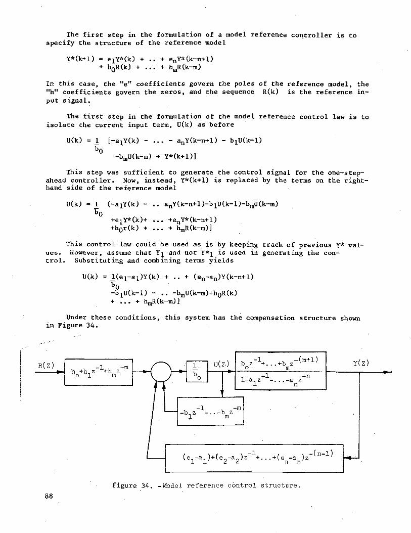
The first step in the formulation of a model reference controller is tospecify the structure of the reference model
Y*(k+l) = eiY*(k) + .. + enY*(k-n+l)+ hQR(k) + . . .
In this case, the "e" coefficients govern the poles of the reference model, the"h" coefficients govern the zeros, and the sequence R(k) is the reference in-put signal.
The first step in the formulation of the model reference control law is toisolate the current input term, U(k) as before
U(k) = L - bLU(k-l)
o-bU(k-m) + Y*(k+l)]m
This step was sufficient to generate the control signal for the one-step-ahead controller. Now, instead, Y*(k+l) is replaced by the terms on the right-hand side of the reference model
U(k) = 1 (-aiY(k) - .. anYU-n+D-bjUCk-D-bnjUCk-m)b0
+e1Y*(k)+ ... +enY*(k-n+l)+h0r(k) + ... + hjjRCk-m)]
This control law could be used as is by keeping track of previous Y* val-ues. However, assume that ¥]_ and not ¥*j_ is used in generating the con-trol. Substituting and combining terms yields
U(k) = J.(e1-a1)Y(k) + .. + (en-an)Y(k-n+l)b
- .. -bmU(k-m)+h0R(k)+ ... +
Under these conditions, this system has the compensation structure shownin Figure 34.
R ( Z )h +hnz~1+h zo 1 m
u(z) m, -1 -n1-a., z -. . . -a z
1 n
-1 , -m-v --v
(e a1)+(e.-aJz-1+...+(e -a1 1 2 2 n n
Y(Z)
Figure 34. -Model reference control structure.
88
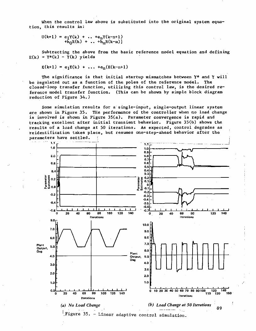
When the control law above is substituted into the original system equa-tion, this results in:
. +enY(k-n+l)
.. +hmR(k-m)]+h0R(k)
Subtracting the above from the basic reference model equation and definingE(k) = Y*(k) - Y(k) yields
= e]E(k) +en(E(k-n+l)
The significance is that initial startup mismatches between Y* and Y willbe regulated out as a function of the poles of the reference model. Theclosed-loop transfer function, utilizing this control law, is the desired re-ference model transfer function. (This can be shown by simple block diagramreduction of Figure 34. )
Some simulation results for a single-input, single-output linear systemare shown in Figure 35. THe performance of the controller when no load changeis involved is shown in Figure 35(a). Parameter convergence is rapid andtracking excellent after initial transient behavior. Figure 35(b) shows theresults of a load change at 50 iterations. As expected, control degrades asreidentification takes place, but resumes one- step- ahead behavior after the
i Lei. s• ' 1 1 '
1 0
8.0
0.6
0.4
|| 0.2
duJO.O
-0.2
-04
-0.6
lave seLneu.
i i 1 1 ill
j,1.1
0.9
0.70.6n K0.40.3
g 8 °-^»S 0.1l.i oCD tn A i
O.UJ -"•!
-0.2-0.3-0.4
J 1 1 1 1 1 1 1 .0.7
-
TIinv
J~\ "^ft J
y \r
, i i i i i20 40 60 80 100
Iterations120 140 20 40 60 80
Iterations120 140
10.0
9.0
8.0
7.0
6.0PlantOutput, 5.0Deg
4.0
3.0 I
2.0 I
1.0 I
\r
20 40 60 80 100 120 140Iterations
0 10 20 30 40 50 60 70 80 90100 120 140110 130 150
Iterations
(a) No Load Change (b) Load Change at 50 Iterations89
.Figure 35. - Linear adaptive control simulation.
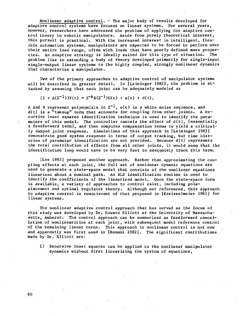
Nonlinear adaptive control. - The major body of results developed foradaptive control systems have focused on linear systems. For several years,however, researchers have addressed the problem of applying the adaptive con-trol theory to robotic manipulators. Aside from purely theoretical interest,this pursuit is practical. With the increased interest in intelligent, flex-ible automation systems, manipulators are expected to be forced to perform overtheir entire load range, often with loads that have poorly defined mass proper-ties. An adaptive strategy is ideally suited for this type of situation. Theproblem lies in extending a body of theory developed primarily for single-inputsingle-output linear systems to the highly coupled, strongly nonlinear dynamicsthat characterize a manipulator.
Two of the primary approaches to adaptive control of manipulator systemswill be described in greater detail. In [Leininger 1983], the problem is at-tacked by assuming that each joint can be adequately modeled as
(1 + A(Z~1))Y(t) = Z-kB(Z-L)U(t) + e(t) + d( t) .
A and B represent polynomials in Z~ , e(t) is a white noise sequence, andd(t) is a "takeup" term that accounts for coupling from other joints. A re-cursive least squares identification technique is used to identify the para-meters of this model. The controller cancels the effect of d(t), (essentiallya feedforward term), and then computes compensation terms to yield a critical-ly damped joint response. Simulations of this approach in [Leininger 1983]demonstrate good system response in terms of output tracking, but time hist-ories of parameter identification are not provided. Because d(t) representsthe total contribution of effects from all other joints, it would seem that theidentification loop would have to be very fast to adequately track this term.
[Lee 1982] proposed another approach. Rather than approximating the cou-pling effects at each joint, the full set of nonlinear dynamic equations areused to generate a state-space model that consists of the nonlinear equationslinearized about a nominal path. An RLS identification routine is used toidentify the coefficients of the linearized model. Once the state-space formis available, a variety of approaches to control exist, including pole-placement and optimal regulator theory. Although not referenced, this approachto adaptive control is reminiscent of that proposed in [Kreisselmeier 1981] forlinear systems.
The nonlinear adaptive control approach that has served as the focus ofthis study was developed by Dr. Howard Elliott at the University of Massachu-setts, Amherst. The control approach can be summarized as feedforward cancel-lation of nonlinear it ies at each joint, with subsequent model reference controlof the remaining linear terms. This approach to nonlinear control is not newand apparently was first used in [Hemami 1982], The significant contributionsmade by Dr. Elliott are:
1) Recursive least squares can be applied to the nonlinear manipulatordynamics without first linearizing the system of equations,
90
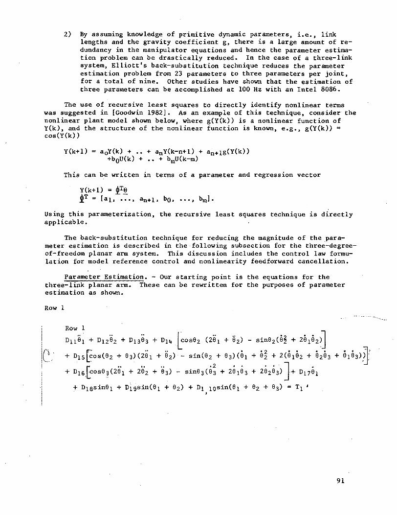
2) By assuming knowledge of primitive dynamic parameters, i.e., linklengths and the gravity coefficient g, there is a large amount of re-dundancy in the manipulator equations and hence the parameter estima-tion problem can be drastically reduced. In the case of a three-linksystem, Elliott's back-substitution technique reduces the parameterestimation problem from 23 parameters to three parameters per joint,for a total of nine. Other studies have shown that the estimation ofthree parameters can be accomplished at 100 Hz with an Intel 8086.
The use of recursive least squares to directly identify nonlinear termswas suggested in [Goodwin 1982]. As an example of this technique, consider thenonlinear plant model shown below, where g(Y(k)) is a nonlinear function ofY(k), and the structure of the nonlinear function is known, e.g., g(Y(k)) =cos(Y(k))
Y(k+l) = a0Y(k) + .. + anY(k-n+l) + an+ig(Y(k))+b0U(k) + .. + bmU(k-m)
This can be written in terms of a parameter and regression vector
> an+l> bO> •••» bmJ•
Using this parameterization, the recursive least squares technique is directlyapplicable.
The back-substitution technique for reducing the magnitude of the para-meter estimation is described in the following subsection for the three-degree-of-freedom planar arm system. This discussion includes the control law formu-lation for model reference control and nonlinearity feedforward cancellation.
Parameter Estimation. - Our starting point is the equations for thethree-link planar arm. These can be rewritten for the purposes of parameterestimation as shown.
Row 1
Row 1r . . . . .2 . . ~|
D l l ^ l ~*~ ^12^2 "*" ^13®3 ~^~ ^l1* cos62 (20^ + 02) — sin02(02 + 20 j0 2 ) |
(\~ + D15Fcos(02 + 03X20]. + 62) - sin(02 + 0 3 ) ( 0 i + 0| + 2(0!02 4- 0203 + 010s)) f
E . . . . . . .2 • • • • " "1:os03(201 + 202 + 03) - sin63(03 + 2 0 X 0 3 + 20203) •
+ Digsin0} + Digsin(0^ + 02) + D\ igsin(0i + 02 +
91
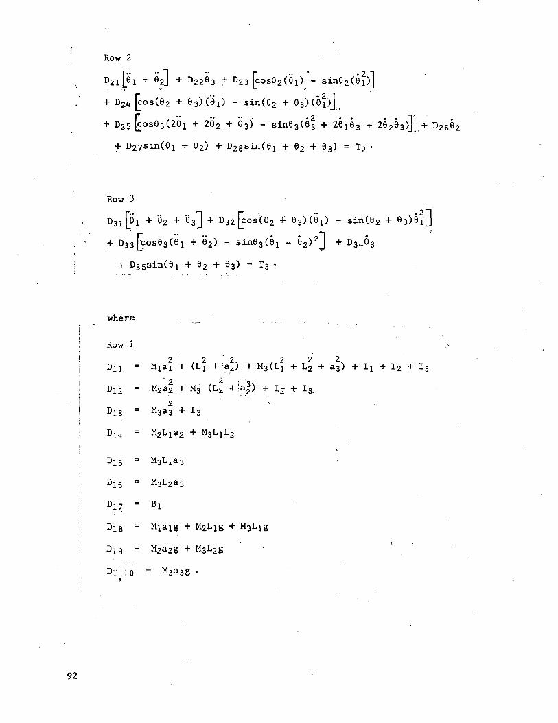
Row 2
r~« • • • ^ ** r * *PTD2 i [_6i + 62J + D2263 + D23 [cos02(0'i) - sin02(e!)J
E « 2 ~I:os(62 + 63) (0J.) - sin(62 + 83) (61)
J>-
+ 025(00363(261 + 262 + 03) - sine3(03 + 26J63 + 26263)] + D2662
+ 62) + D28sin(91 + 02 + 63) = T2 •
Row 3
«2- .. .. n r ••pl + 62 + 63J + D32[cos(62 + 63)(01) - sin(62
E " • • o~i:os63(e1 + 62) - 3 63(6! - 62)
2J + 03463
4- 03581.11(6! + 62 + 63) = T3 «
wherei - - - - - -
; Row i! 2 2 T 2 2 2 2I DH = Miai + (Li + ;a2) + M3(L1 + L2 + a3) + l± + I2 + I3
2 2 ,'-?D12 = .M2a2.+ M3 (L2 -Ha|) + I2 + I3
2 ' \D13 = M3a3 + I3
= M3L2a3
Di7 = Bl
D19 = M2a2g +
DI 10 = M3a38
92
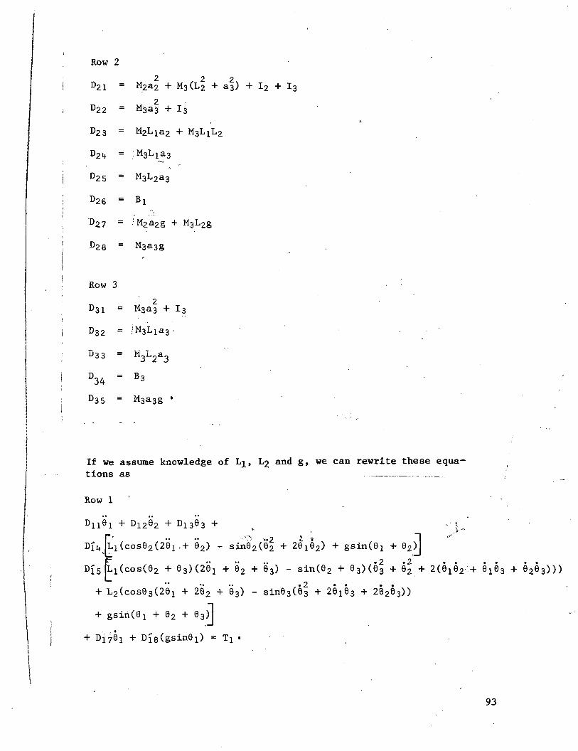
Row 2
D21 =
D22 =
2M2a2
2M3(L2
2a3) I2 + I3
M3a3 +13
25 = M3L2a3
D26
D28 =
: M2a2g + M3L2g
M3a3g
Row 3
2D31 = M3a3 + I3
D32 = ;M3L!a3.
D33 = M3L2a3
D_ . = B334 3
D35 = M3a3g •
If we assume knowledge of Lit L2 and g, we can rewrite these equations as ._. ........... - ____ ...... __
Row 1
L1(cos92(291 .
L^(cos(02 +
+ L2(cos03(201
+ Di70! +
92) - sin02(02 + 29j92) + gsin(0j + 92)
92 + e'3) - sin(02 + 03)(93 + 92 +
202 + 03) - sin03(03 + 20103 + 20203))
03)]
93
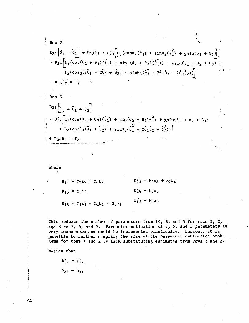
: Row 2
.. -| .. r .. .2 -|+ 62 I + D2293 + D23|LI(cos92(6i) + sin62(6j) + gsin(9i + 62)
_ -1 L _hI "* O
+ D21 tlL1(cos(92 + eaXOi ) + sin (02 + 9 3 ) (0 1 ) ) + gsinOx + 92 + 63) +
..L2(cos3(201 + 262 + 63) - sin03(93 + 29x93 + Z^S^))
+ T\ ~fa — T*U2go2 — T2
Row 3
^ i fS i + 92 + 93~lL™ ^J "
r " • 2+ D3 2 lLi(cos(92 + 93)(9!) + sin(92 + 83)6!) + gsin(6i 4- 62 + 63)
U. , _/ • • • • • • • • 2
+ L2(.cos63(91 + 92) + sin93(9i + 26i92 + 62))
+ D31t93 = T3
where
jit = M2a2 + M3L2 D23 = M2a2
M3a3 D2i+ = M3a3
This reduces the number of parameters from 10, 8, and 5 for rows 1, 2,and 3 to 7, 5, and 3. Parameter estimation of 7, 5, and 3 parameters isvery reasonable and could be implemented practically. However, it ispossible to further simplify the size of the parameter estimation prob-lems for rows 1 and 2 by back-substituting estimates from rows 3 and 2.
Notice that
D22 = D31
94
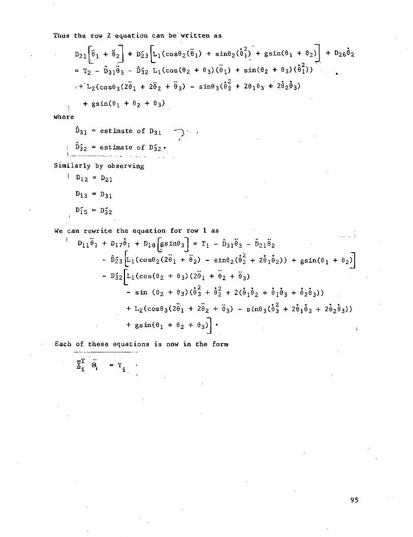
Thus the row 2 equation can be written as
D21 pi + 82 + D23 L1(cos62(ei) + sin62(0i) 4- gsin(9i + 92) + D2602
= T2 - D3i'e3 - D§2 L1(cos(62 + 03)(0i) + sin(62 + 83) (0!)
1+ 2(00883(26! + 28*2 + 63) - sin93(03 + 20163 * 28293)
Oi + 82 + 83)
where
D31 = estimate of D31 -~~V/;w
i D32 = estimate of D32•
Similarly by observing
I D12 = D2i
D13 = D31
We can rewrite the equation for row 1 as
L1(cos02(201 + 02) - sin02(02 + 20102)) + gsin(6i + 02)
L1(cos(92 + 8 3) (28'i + 02 + 83)
• -2 .2- sin (92 + 03)(03 + 02 + 2(6192 + 0^3 + 9293))
+ L2(cose3(20'1 + 282 + 83) - sin03(03 + 20^3 + 20293))
+ gsin(0! + 02 + ©3)I •
Each of these equations is now in the form
_X *-
95
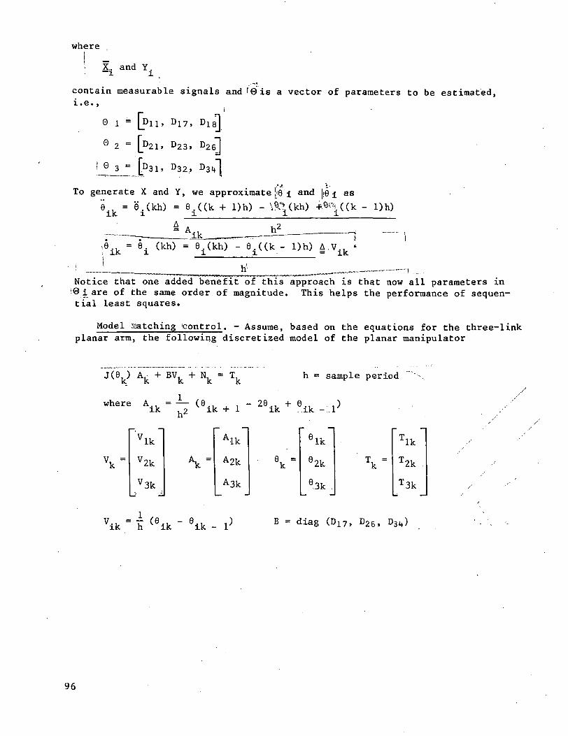
where
1 X. and Y.
contain measurable signals and I ©is a vector of parameters to be estimated,i.e.,
0 i =
0 2 =
, D l7 ,
D23, D26~]
'_^£J [D31, D32, D3lt~[
f t j> ' ~ 'To generate X and Y, we approximate ,16 i and Ij0 j as
e±k = e..(kh) = e ± ( (k
ik= e± (kh) = e±(kh) - e± ( (k -
h-Notice that one added benefit of this approach is that now all parameters in'©i are of the same order of magnitude. This helps the performance of sequen-tial least squares.
Model matching icontrol. - Assume, based on the equations for the three-linkplanar arm, the following discretized model of the planar manipulator
J(9, ) A.k k
BV. + N. = T,k k k
h = sample period
where A.. = — (9 - 26 + 6 . ')ik ,2 ik + 1 ik . ik -..1
"vlk"V2k
73k,\ =
" Alk"A2k
A3k
9k =
'6lk"
9 2k
93k .
\ =
"Tlk"
T2k .
T3k
vik • h (eik - eik - B = diag (D17, D26, D3lf)
96

J(6.) =
•
2D1itcos62l, \ /D12 + D1£fcose2
\ f•f 2D15cos(82k + 63k)| | + D15cos(82k
2D16cos83k / \+ 2D.16cos83
• 2D25cos63,Iv
-I- D33cos83IX
'N.
- D16
+ D25 [-
«3k = -D32^sin(62k H
Assume we want the closed-loop system to be characterized by the model
Eneik + i + Ei26ik + E13elk _ l = Hllrlk + H12rlk _
I + E22e2k•+ E23e2k _ 1 = H21r2k + H22r2k _
+ E3382k _ 1
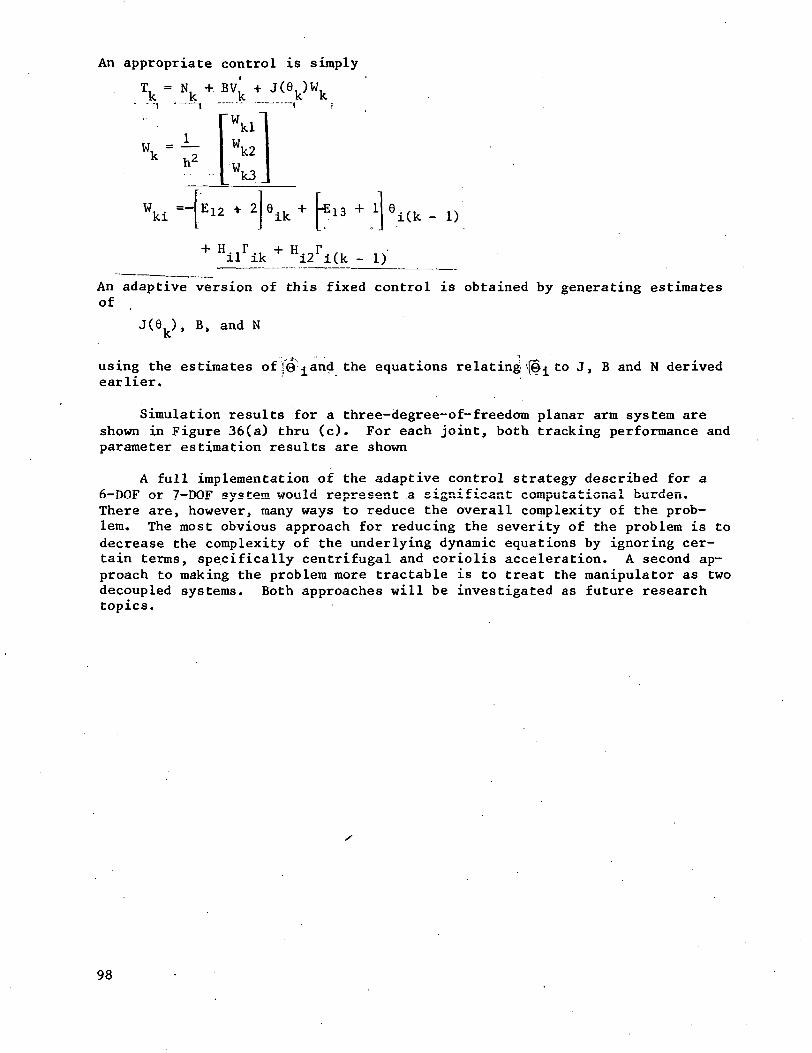
An appropriate control is simply
. T, = N. + BV.' + J(6. )W.k k k k k
w. = —k h2"wkl"
Wk2
2 e.k U13 + 16.,,p1 i(k
Hiirik + Hi2ri(k -
An adaptive version of this fixed control is obtained by generating estimatesof
J(6 ), B, and NiC
using the estimates of^^and the equations relating' <(@ to J, B and N derivedearlier.
Simulation results for a three-degree-of-freedom planar arm system areshown in Figure 36(a) thru (c). For each joint, both tracking performance andparameter estimation results are shown
A full implementation of the adaptive control strategy described for a6-DQF or 7-DOF system would represent a significant computational burden.There are, however, many ways to reduce the overall complexity of the prob-lem. The most obvious approach for reducing the severity of the problem is todecrease the complexity of the underlying dynamic equations by ignoring cer-tain terms, specifically centrifugal and coriolis acceleration. A second ap-proach to making the problem more tractable is to treat the manipulator as twodecoupled systems. Both approaches will be investigated as future researchtopics.
98
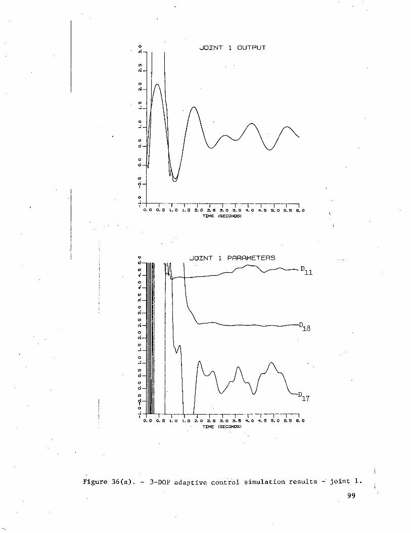
JOINT 1 OUTPUT
I I I I I T 1 IO. O O. S 1. O l.S 2. O 2.5 3. O 3.5 •». O •». S S. O S. S 6. O
TIME (SECONDS)
JOINT 1 PRRRMETERS
I I I I I I I \ 1O. O O. 5 1. O l.S 2. O 2. S 3. O 3. S
TIME (SECONDS)
Figure 36(a). - 3-DOF adaptive control simulation results - joint 1,
99
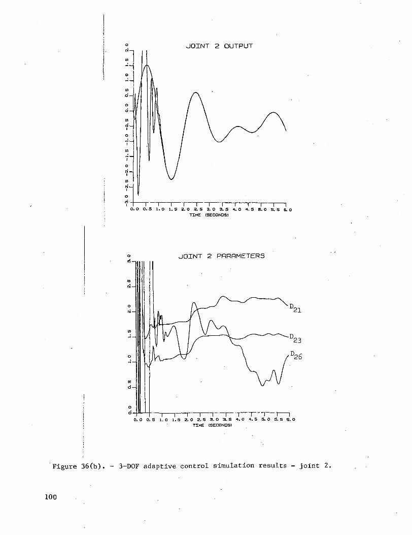
JOINT 2 OUTPUT
O. O O. S 1. O 1. 5 2. O 2.5 3. O 3.5 4. O 4. 5 S. 0 5. S 6. OTIME (SECONDS)
JOINT 2 PRRRMETERS
0. O O. S 1. O 1.5 2. O 2. S 3. O 3. S 4. O 4.5 S. O S. S 6. O
Figure 36(b). - 3-DOF adaptive control simulation results - joint 2.
100
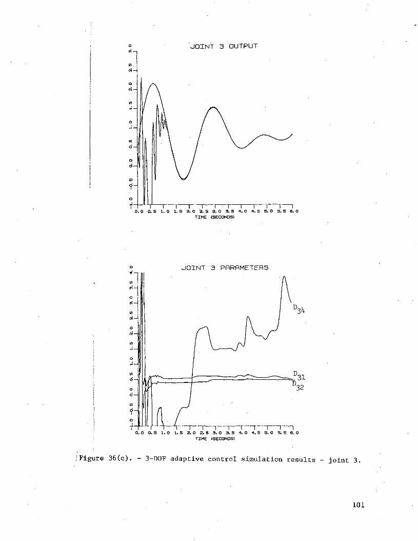
JOINT 3 OUTPUT
O. O O. S 1. O 1. S 2.0 2.5 3. O 3. S 4. O 4. 5 S. O S. S 6. OTIME (SECONDS)
JOINT 3 PRRRMETERS
~T 1"1 I 1 I"0.0 O. S 1.0 1. S 2.0 2.5 3.0 3.5 •*. O 4.5 5. O 5. S 6. O
TIME (SECONDS)
[Figure 36(c). - 3-DOF adaptive control simulation results - joint 3,
101
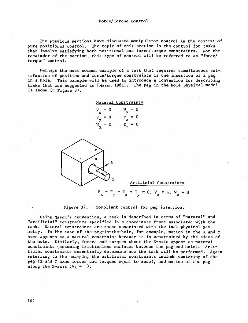
Force/Torque Control
The previous sections have discussed manipulator control in the context ofpure positional control. The topic of this section is the control for tasksthat involve satisfying both positional and force/torque constraints. For theremainder of the section, this type of control will be referred to as "force/torque" control.
Perhaps the most common example of a task that requires simultaneous sat-isfaction of position and force/torque constraints is the insertion of a pegin a hole. This example will be used to introduce a convention for describingtasks that was suggested in [Mason 1981]. The peg-in-the-hole physical modelis shown in Figure 37..
Natural Constraints
V = 0xV = 0yw = ox
W = 0yF = ozT = 0z
Artificial Constraints
T = T = 0, V = a, W = 0x y z ' z
Figure 37. - Compliant control for peg insertion.
Using Mason's convention, a task is described in terms of "natural" and"artificial" constraints specified in a coordinate frame associated with thetask. Natural constraints are those associated with the task physical geo-metry. In the case of the peg-in-the-hole, for example, motion in the X and Yaxes appears as a natural constraint because it is constrained by the sides ofthe hole. Similarly, forces and torques about the Z-axis appear as naturalconstraints (assuming frictionless surfaces between the peg and hole). Arti-ficial constraints essentially determine how the task will be performed. Againreferring to the example, the artificial constraints include centering of thepeg (X and Y axes forces and torques equal to zero), and motion of the pegalong the Z-axis (Vz = ).
102
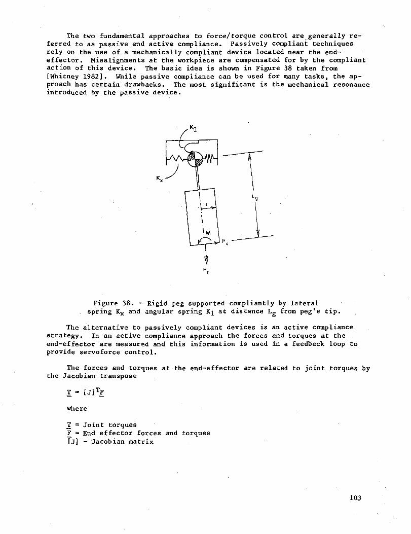
The two fundamental approaches to force/torque control are generally re-ferred to as passive and active compliance. Passively compliant techniquesrely on the use of a mechanically compliant device located near the end-effector. Misalignments at the workpiece are compensated for by the compliantaction of this device. The basic idea is shown in Figure 38 taken from[Whitney 1982], While passive compliance can be used for many tasks, the ap-proach has certain drawbacks. The most significant is the mechanical resonanceintroduced by the passive device.
Figure 38, - Rigid peg supported compliantly by lateralspring Kx and angular spring K^ at distance Lg from peg's tip.
The alternative to passively compliant devices is an active compliancestrategy. In an active compliance approach the forces and torques at theend-effector are measured and this information is used in a feedback loop toprovide servoforce control.
The forces and torques at the end-effector are related to joint torques bythe Jacobian transpose
T = [J]TF
where
T^ = Joint torquesF = End effector forces and torques[j] - Jacobian matrix
103
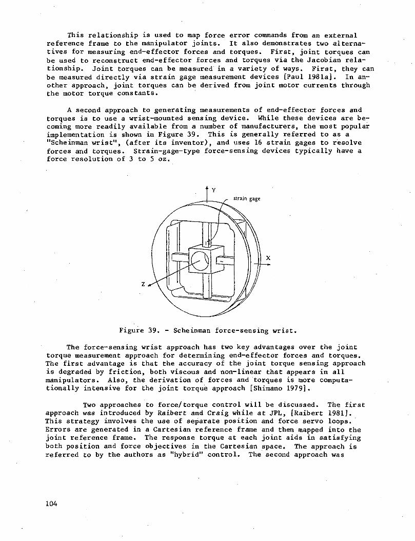
This relationship is used to map force error commands from an externalreference frame to the manipulator joints. It also demonstrates two alterna-tives for measuring end-effector forces and torques. First, joint torques canbe used to reconstruct end-effector forces and torques via the Jacobian rela-tionship. Joint torques can be measured in a variety of ways. First, they canbe measured directly via strain gage measurement devices [Paul 1981a]. In an-other approach, joint torques can be derived from joint motor currents throughthe motor torque constants.
A second approach to generating measurements of end-effector forces andtorques is to use a wrist-mounted sensing device. While these devices are be-coming more readily available from a number of manufacturers, the most popularimplementation is shown in Figure 39. This is generally referred to as a"Scheinman wrist", (after its inventor), and uses 16 strain gages to resolveforces and torques. Strain-gage-type force-sensing devices typically have aforce resolution of 3 to 5 oz.
strain gage
Figure 39. - Scheinman force-sensing wrist.
The force-sensing wrist approach has two key advantages over the jointtorque measurement approach for determining end-effector forces and torques.The first advantage is that the accuracy of the joint torque sensing approachis degraded by friction, both viscous and non-linear that appears in allmanipulators. Also, the derivation of forces and torques is more computa-tionally intensive for the joint torque approach [Shimano 1979].
Two approaches to force/torque control will be discussed. The firstapproach was introduced by Raibert and Craig while at JPL, [Raibert 1981],This strategy involves the use of separate position and force servo loops.Errors are generated in a Cartesian reference frame and then mapped into thejoint reference frame. The response torque at each joint aids in satisfyingboth position and force objectives in the Cartesian space. The approach isreferred to by the authors as "hybrid" control. The second approach was
104
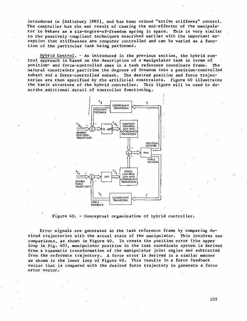
introduced in [Salisbury 1980], and has been coined "active stiffness" control.The controller has the net result of causing the end-effector of the manipula-tor to behave as a six-degree-of-freedom spring in space. This is very similarto the passively compliant techniques described earlier with the important ex-ception that stiffnesses are computer controlled and can be varied as a func-tion of the particular task being performed.
Hybrid Control. - As introduced in the previous section, the hybrid con-trol approach is based on the description of a manipulator task in terms ofposition- and force-controlled axes in a task reference coordinate frame. Thenatural constraints partition the degrees of freedom into a position-controlledsubset and a force-controlled subset. The desired position and force trajec-tories are then specified by the artificial constraints. Figure 40 illustratesthe basic structure of the hybrid controller. This figure will be used to de-scribe additional detail of controller functioning.
C i*d + ;'V^\
DESIREDPOSITION
Cff« + /-
~*}fi
^DESIRED /FORCETRAJECTORY
Cx
POSITIONFEEDBACK
J ^
y=C>[ii-i^
p=C> i i
c£
FORCE .
i
~*L CONTROL] Z±> LAW AND
COORDINATE
POSITIONSENSORS
V + '(LJ==> ARMXt
1 f FORCESENSORS
, CF FORCE"" CONTROL
J) LAW ANDCOORDINATE
F
1
t
Figure 40. - Conceptual organization of hybrid controller.
Error signals are generated in the task reference frame by comparing de-sired trajectories with the actual state of the manipulator. This involves twocomparisons, as shown in Figure 40. To create the position error (the upperloop in Fig. 40), manipulator position in the task coordinate system is derivedfrom a kinematic transformation of the manipulator joint angles and subtractedfrom the reference trajectory. A force error is derived in a similar manneras shown in the lower loop of Figure 40. This results in a force feedbackvector that is compared with the desired force trajectory to generate a forceerror vector.
105
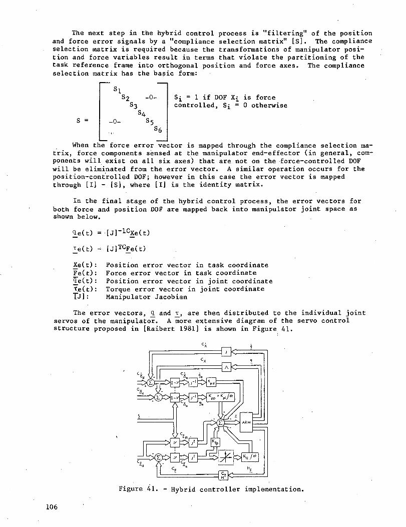
The next step in the hybrid control process is "filtering" of the positionand force error signals by a "compliance selection matrix" [SJ. The complianceselection matrix is required because the transformations of manipulator posi-tion and force variables result in terms that violate the partitioning of thetask reference frame into orthogonal position and force axes. The complianceselection matrix has the basic form:
S =
SiS2 -0-S3S4
-0-S6
S£ = 1 if DOFcontrolled, S-;
is force0 otherwise
When the force error vector is mapped through the compliance selection ma-trix, force components sensed at the manipulator end-effector (in general, com-ponents will exist on all six axes) that are not on the -force-controlled DOFwill be eliminated from the error vector. A similar operation occurs for theposition-controlled DOF; however in this case the error vector is mappedthrough [I] - [S], where [I] is the identity matrix.
In the final stage of the hybrid control process, the error vectors forboth force and position DOF are mapped back into manipulator joint space asshown below.
le(t) = [J]-lcXe(t)
l«(t) = [JJTGFe(t)
Xe(t): Position error vector in task coordinateFe(t): Force error vector in task coordinateQ_e(t): Position error vector in joint coordinateTe(t): Torque error vector in joint coordinateTJ]: Manipulator Jacobian
The error vectors, <1 and T_, are then distributed to the individual jointservos of the manipulator. A more extensive diagram of the servo controlstructure proposed in [Raibert 1981] is shown in Figure 41.
Figure 41. - Hybrid controller implementation.
106
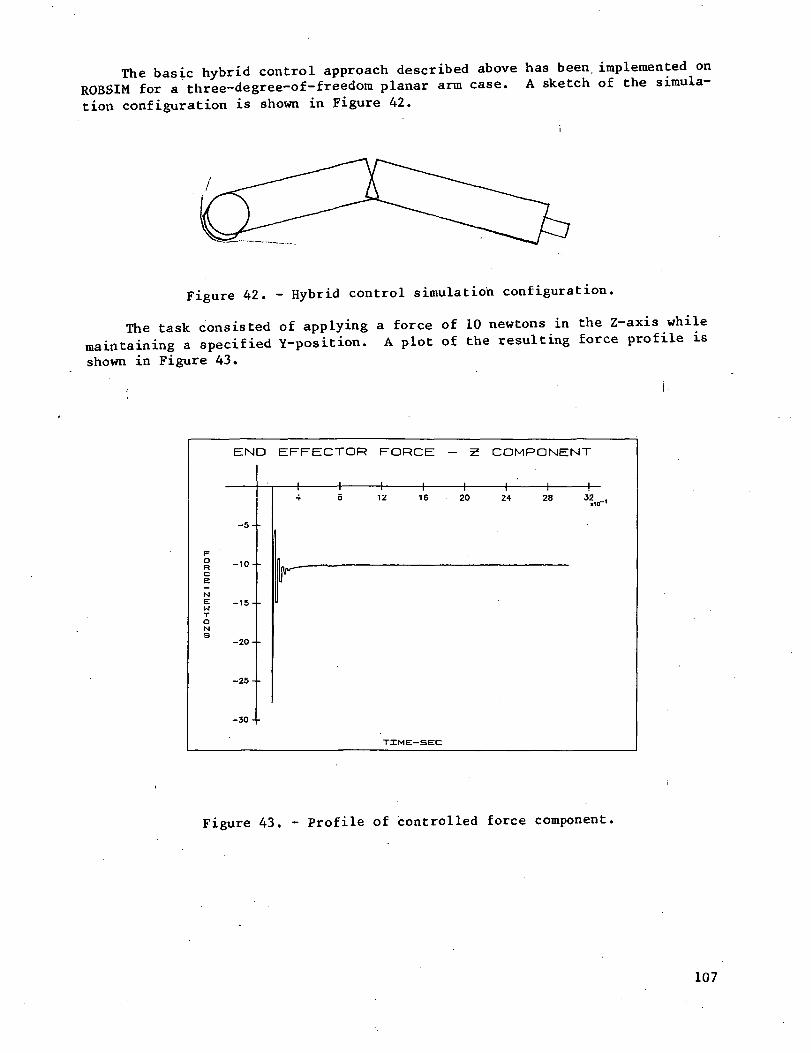
The basic hybrid control approach described above has been, implemented onROBSIM for a three-degree-of-freedom planar arm case. A sketch of the simula-
tion configuration is shown in Figure 42.
Figure 42. - Hybrid control simulation configuration.
The task consisted of applying a force of 10 newtons in the Z-axis whilemaintaining a specified Y-position. A plot of the resulting force profile is
shown in Figure 43.
END EFFECTOR FORCE - COMPONENT
oR
WTONS
-5- •
-10--
-15- -
-20--
-25--
-30--
16 20
TIME-SEC
24 28Hnr-
Figure 43. - Profile of controlled force component.
107
Active stiffness control. - The concept of active stiffness control, hasmany of the attributes of the hybrid control strategy described earlier, butintroduces the novel concept of forcing the end-effector of the manipulator tobehave as a six-dimensional spring in the Cartesian reference frame. Aspointed out earlier, this bears a striking resemblance to passive complianceapproaches in terms of accommodating misalignments between the end effector andtask. Again, the important difference is that in an active compliance ap-proach, stiffnesses on specific axes are controlled externally and variedduring different phases of a task. For example, during rapid slewing motionsin moving from point to point, stiffnesses can be set high to minimize reac-tions to acceleration- induced forces from the load or tool.
To arrive at an equivalent six-dimensional spring relationship expressedin terms of joint displacements and joint torques
T = [J]TK[J]<59
The matrix K^ = JTKJ is referred to as the joint stiffness matrix. Thepoint in the hand reference frame that serves as the basis for the computationof the Jacobian is referred to as the stiffness center. This is the point atwhich pure forces cause only translation and pure torques cause only rotation.
In its most basic form active stiffness control can be implemented by gen-erating joint torque commands of the form
The term TJJ is a bias torque generated from the relationship TR = JTFR.
FJJ represents bias forces in the Cartesian reference frame. Note that theappropriate choice of K leads to a decomposition of force- and position-controlled axes as in the hybrid control scheme.
A six-dimensional linear spring is described by the relationship
F = [K]6X
6X is a generalized displacement from a nominal position XQ of the hand ori-gin and consists of three orthogonal translation components and three small rotations about orthogonal axes. This diagonal matrix [Kj contains the springcoefficients for each axis.
The Cartesian displacement .<$ X can be related to a manipulator joint dis-placement 69, (<S6_ = 9_ - 9_Q) through the Jacobian matrix
6X = [J]60
Joint torques are also related to end-effector forces and torques as afunction of the Jacobian
T = [J]TF
108
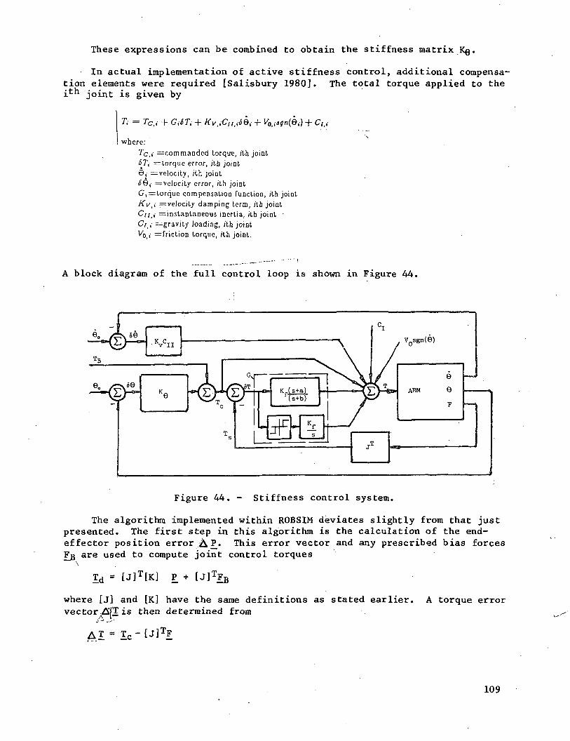
These expressions can be combined to obtain the stiffness matrix Kg.
In actual implementation of active stiffness control, additional compensa-tion elements were required [Salisbury 1980]. The total torque applied to theit" joint is given by
where:TC,I ^commanded torque, /th jointST{ = torque error, /th joint9, —velocity, /th joint(59,- =vclocity error, /th jointG,=torq'ue compensation funct ion, /th jointKy t{ ^velocity damping term, y'tb jointC^yy.i ^instantaneous inert ia, /th joint •Ctt{ =gravity loading, /th jointVQ ,- =fr ict ion torque, /th joint.
A block diagram of the full control loop is shown in Figure 44.
Figure 44. - Stiffness control system.
The algorithm implemented within ROBSIM deviates slightly from that justpresented. The first step in this algorithm is the calculation of the end-effector position error & P_. This error vector and any prescribed bias forcesFJJ are used to compute joint control torques
Td = [J]T[K] p + [J FB
where [j] and [K] have the same definitions as stated earlier. A torque errorvector AfT is then determined from
A,!*"
A.I = lc
109
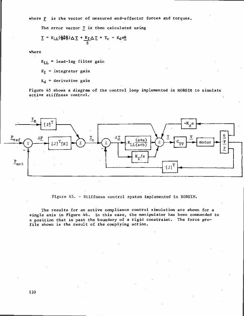
where F_ is the vector of measured end-effector forces and torques.
The error vector T is then calculated using
where
KLL = lead-lag filter gain
Kj = integrator gain
K<j = derivative gain
Figure 45 shows a diagram of the control loop implemented in ROBSIM to simulateactive stiffness control.
; K /s
fT1
TJ11L J J
1
f — i
Figure 45. - Stiffness control system implemented in ROBSIM.
The results for an active compliance control simulation are shown for asingle axis in Figure 46. In this case, the manipulator has been commanded toa position that is past the boundary of a rigid constraint. The force pro-file shown is the result of the complying action.
110
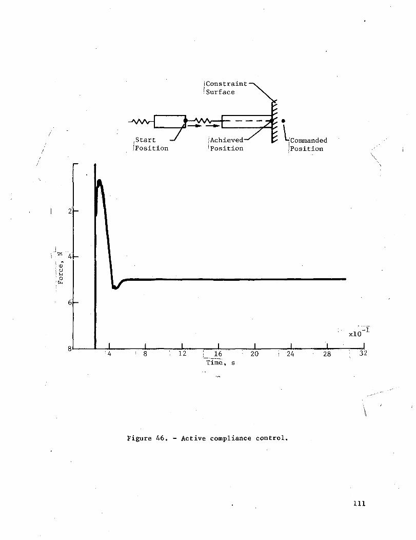
;Start'Position
(Constraint'I Surface
jAchieved-'Position
a,\s ^Commanded•Position
xlO-1
12 16 20Time, s
24
Figure 46. - Active compliance control.
28 32
111
MANIPULATOR TRAJECTORY PLANNING
Manipulator systems often must operate in environments "cluttered" withobstacles, e.g., the objects being manipulated and the machinery with which thearms are interfacing. When performing tasks, the motions of the arms must becarefully planned to avoid collisions between the manipulator links and theseobstacles. Collisions between the various parts of the manipulator system mustalso be prevented, especially in multiple-arm systems or when manipulatingbulky objects. Manipulator path-planning can also be used to improve task per-formance by finding paths that minimize energy consumption or operation time,or that avoid singular configurations of the arm, etc.
To date, path-planning research has focused on two application areas—paths for polyhedral objects and paths for robotic manipulators. Polyhedralobjects are self-contained—mobile objects such as autonomous robotic ve-hicles,* aircraft, etc. The obvious difference between such an object and amanipulator is that the latter is not "mobile" in the sense that one end isfixed to a platform or base that may be mobile. A manipulator arm is a com-bination of connected links, each of which is a polyhedron. The "motion" of amanipulator is constrained by the link connectivity, which limits its overallreach. The volume (or area) reachable by the hand or tool is a manipulator'sworking envelope. When a manipulator moves, each of its links sweeps out thepath of a polyhedron. Thus, path planning for the motion of polyhedral objectsis a subproblem in trajectory planning for manipulators.
The problem of planning paths for polyhedrals has received much attention,with the intent of generalizing methods to manipulator path planning. Unfor-tunately, the two problems have inherent differences, limiting the applicationof polyhedral methods to the manipulator case. There have been implementationsof manipulator path planners relying solely on relations among polyhedral ob-jects and the polyhedral components of the arm [Brooks 1983b] but these neithercapitalize on the serial nature of the manipulator arm nor provide for diversemanipulator operations. They have also demonstrated success only in very sim-ple environments composed of rectangular polyhedrals.
This section of the report discusses the current state of path-plannertechnology, with the emphasis on path planning for robotic manipulators. Thefirst part consists of the history and development of path-planning methods forboth mobile objects and manipulators. The next subsection examines currenttechnology and describes the results of path-planning research under the ROBSIMcontract. Finally, the third part compares the current methods and providessome topics for further study. The emphasis in this work is on path planningto avoid obstacles in the manipulator's operating environment. Table IV sum-marizes the notation employed in this section.
* SRI's Shakey and the Mars rover are two examples of such vehicles.
112
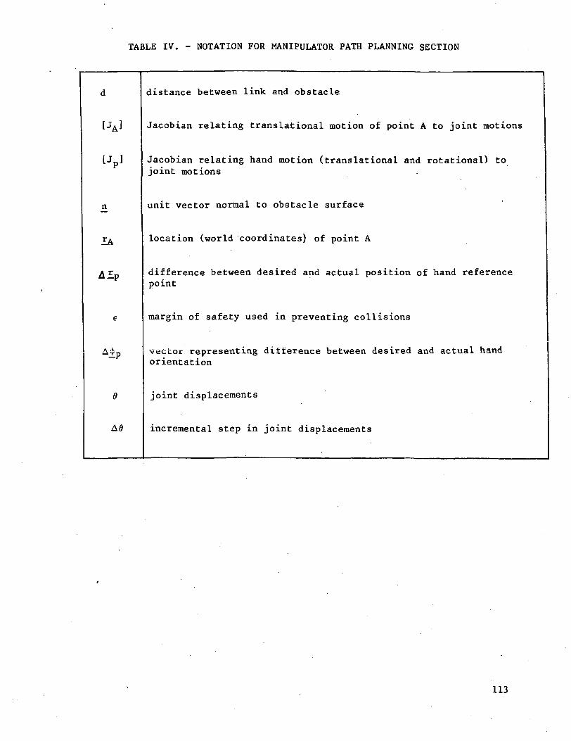
TABLE IV. - NOTATION FOR MANIPULATOR PATH PLANNING SECTION
Up]
distance between link and obstacle
Jacobian relating translational motion of point A to joint motions
Jacobian relating hand motion (translational and rotational) tojoint motions
unit vector normal to obstacle surface
location (world coordinates) of point A
difference between desired and actual position of hand referencepoint
margin of safety used in preventing collisions
vector representing difference between desired and actual handorientation
joint displacements
incremental step in joint displacements
113
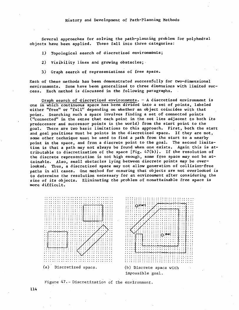
History and Development of Path-Planning Methods
Several approaches for solving the path-planning problem for polyhedralobjects have been applied. These fall into three categories:
1) Topological search of discretized environments;
2) Visibility lines and growing obstacles; -
3) Graph search of representations of free space.
Each of these methods has been demonstrated successfully for two-dimensionalenvironments. Some have been generalized to three dimensions with limited suc-cess. Each method is discussed in the following paragraphs.
Graph search of discretized environments. - A discretized environment isone in which continuous space has been divided into a set of points, labeledeither "free" or "full" depending on whether an object coincides with thatpoint. Searching such a space involves finding a set of connected points("connected" in the sense that each point in the set lies adjacent to both itspredecessor and successor points in the world) from the start point to thegoal. There are two basic limitations to this approach. First, both the startand goal positions must be points in the discretized space. If they are not,some other technique must be used to find a path from the start to a nearbypoint in the space, and from a discrete point to the goal. The second limita-tion is that a path may not always be found when one exists. Again this is at-tributable to discretization of the space [Fig. 47(b)]. If the resolution ofthe discrete representation is not high enough, some free space may not be at-tainable. Also, small obstacles lying between discrete points may be over-looked. Thus, a discretized space may not allow generation of collision-freepaths in all cases. One method for ensuring that objects are not overlooked isto determine the resolution necessary for an environment after considering thesize of its objects. Eliminating the problem of nonattainable free space ismore difficult.
(a) Discretized space. (b) Discrete space with
impossible goal.
Figure 47.- Discretization of the environment.
114
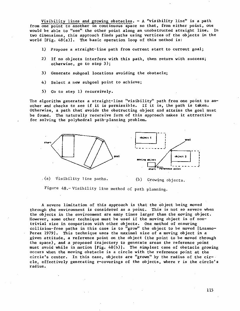
Visibility lines and growing obstacles. - A "visibility line" is a pathfrom one point to another in continuous space so that, from either point, onewould be able to "see" the other point along an unobstructed straight line. Intwo dimensions, this approach finds paths using vertices of the objects in theworld [Fig. 48(a)]. The basic operation loop of this method is:
1) Propose a straight-line path from current start to current goal;
2) If no objects interfere with this path, then return with success;otherwise, go to step 3);
3) Generate subgoal locations avoiding the obstacle;
4) Select a new subgoal point to achieve;
5) Go to step 1) recursively.
The algorithm generates a straight-line "visibility" path from one point to an-other and checks to see if it is permissible. If it is, the path is taken.Otherwise, a path that avoids the obstructing object and attains the goal mustbe found. The naturally recursive form of this approach makes it attractivefor solving the polyhedral path-planning problem.
seal
goal•oving
reference point
(a) Visibility line paths. (b) Growing objects.
Figure 48.- Visibility line method of path planning.
A severe limitation of this approach is that the object being movedthrough the environment is considered as a point. This is not so severe whenthe objects in the environment are many times larger than the moving object.However, some other technique must be used if the moving object is of non-trivial size in comparison with other objects. One method of ensuringco11is ion-free paths in this case is to "grow" the object to be moved [Lozano-Perez 1979]. This technique uses the maximal size of a moving object in agiven attitude, a reference point on the object (the point to be moved throughthe space), and a proposed trajectory to generate areas the reference pointmust avoid while in motion [Fig. 48(b)]. The simplest case of obstacle growingoccurs when the moving obstacle is a circle with the reference point at thecircle's center. In this case, objects are "grown" by the radius of the cir-cle, effectively generating r-coverings of the objects, where r is the circle'sradius.
115
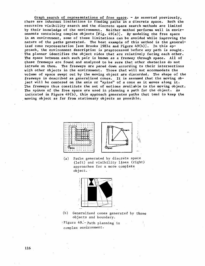
Graph search of representations of free space. - As asserted previously,there are inherent limitations to finding paths in a discrete space. Both therecursive visibility search and the discrete space search methods are limitedby their knowledge of the environment. Neither method performs well in envir-onments containing complex objects [Fig. 49(a)J. By modeling the free spacein an environment, some of these limitations can be avoided while improving thenature of the paths generated. The best example of this method is the general-ized cone representation [see Brooks 1983a and Figure 49(b)]. In this ap-proach, the environment description is preprocessed before any path is sought.The planner identifies the object sides that are relatively facing each other.The space between each such pair is known as a freeway through space. All ofthese freeways are found and analyzed to be sure that other obstacles do notintrude on them. The freeways are pared down according to their intersectionswith other objects in the environment. Those that will not accommodate thevolume of space swept out by the moving object are discarded. The shape of thefreeways is described as generalized cones. It is assumed that the moving ob-ject will be centered on the axis or "spine" of a cone as it moves along it.The freeways thus constitute the set of motions available to the moving object.The spines of the free space are used in planning a path for the object. Asindicated in Figure 49(b), this approach generates paths that tend to keep themoving object as far from stationary objects as possible.
(a) Paths generated by discrete space(left) and visibility lines (right)approaches for a more completeobject.
(b) Generalized cones generated by threeobjects and boundary.
i Figure 49.'-Path planning in ](
complex environment.
116
Path-Planning Research Under the ROBSIM Contract
Three approaches to manipulator path planning were investigated under theROBSIM contract:
1) The generalized cone method;
2) The joint space method;
3) The incremental, constrained-motion method.
Research applied to these methods resulted in preliminary implementations ofeach approach. The following is a discussion of each method, itsimplementation, and the outcome of the research.
The generalized cone method. - A path planner based on the approach deve-loped by Brooks (see [Brooks 1983a and 1983b]) and the previous discussion),in which free space is represented by generalized cones and trajectories alongthe spines of these freeways are generated, was implemented initially. Todecrease the amount of computation involved in the algorithm, some simplifi-cations are imposed on the planning environment. All objects in the environ-ment, including the arm, are assumed to be rectangular in shape and grid-aligned (i.e., their sides are parallel to the sides of the workspace). Thislimitation is not overly restrictive. Irregularly shaped objects can be en-closed within bounding boxes. Few feasible solutions will be excluded by theuse of this approximation, especially considering that this planning algorithmprefers paths that follow wide lanes rather than paths for which the arm barelyfits between obstacles.
Programs for testing the algorithm were also developed. These programsgenerate random obstacles, start points and goal points within a two-dimensional workspace. Any number of objects are allowed in the environment.Four obstacles provide good testing results; with more obstacles, the computa-tion time for preprocessing the environment grows rapidly. This problem is in-herent in the Brooks algorithm but might be circumvented by applying heuristicsto determine which calculations are necessary.
The planner was quite successful in solving the problems it set for it-self. After generating a workspace, it would preprocess the environment,establishing the path freeways, and seek a path from the start toward the goal.Although it found a path in the majority of cases, the paths were sometimesvery indirect. This may be caused by some subtle programming bug yet to be un-covered. The planner is able to rotate the arm as well as translate it, andoccasionally finds intricate paths involving sequences of rotations and trans-lations through several corners.
The joint space method. - Joint space is an N-dimensional vector space,where N is the number of manipulator joints or degrees of freedom, in whicheach coordinate axis corresponds to one joint displacement. Any point in thisspace represents a unique configuration of the manipulator. Similarly, withappropriate bounds on the joint displacements, any configuration of the armcorresponds to a unique vector in joint space. If, for any configuration ofthe manipulator, some link collides with an obstacle (including another link),that configuration is forbidden. In the joint space method of path planning,
117
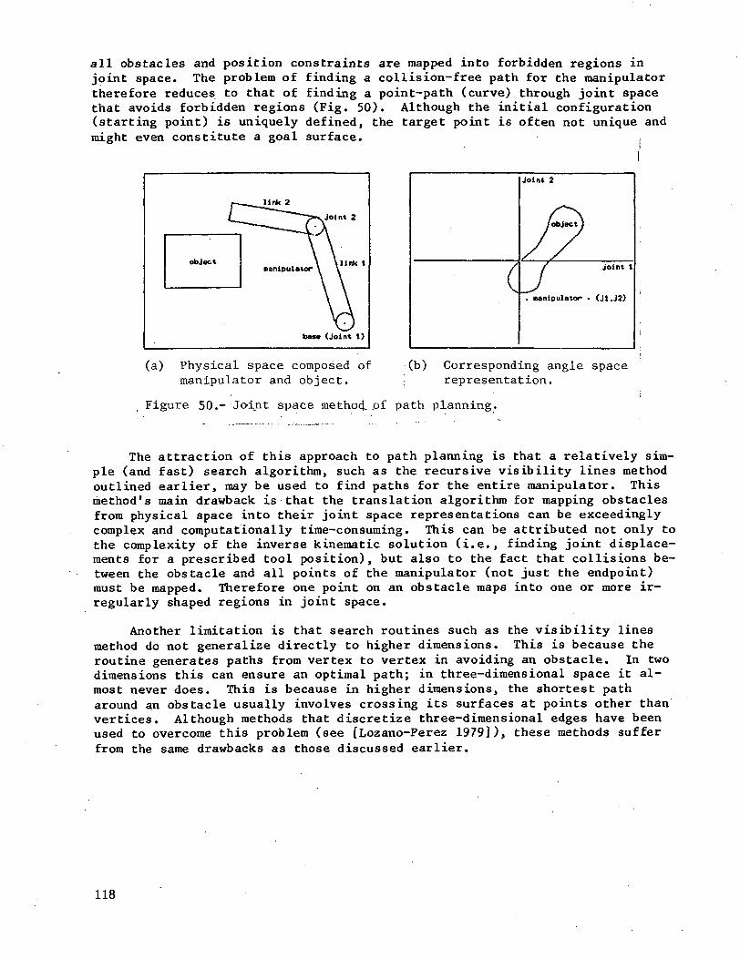
all obstacles and position constraints are mapped into forbidden regions injoint space. The problem of finding a collision-free path for the manipulatortherefore reduces to that of finding a point-path (curve) through joint spacethat avoids forbidden regions (Fig. 50). Although the initial configuration(starting point) is uniquely defined, the target point is often not unique andmight even constitute a goal surface.
link 2
Joint 2
link 1
ban (Joint 1)
(
Joint 2
/object}
/ Joint 1
. Banipulator - (J1.J2)
(a) Physical space composed of (b) Corresponding angle spacemanipulator and object. \ representation.
Figure 50.- Joint space method, .of path planning.
The attraction of this approach to path planning is that a relatively sim-ple (and fast) search algorithm, such as the recursive visibility lines methodoutlined earlier, may be used to find paths for the entire manipulator. Thismethod's main drawback is that the translation algorithm for mapping obstaclesfrom physical space into their joint space representations can be exceedinglycomplex and computationally time-consuming. This can be attributed not only tothe complexity of the inverse kinematic solution (i.e., finding joint displace-ments for a prescribed tool position), but also to the fact that collisions be-tween the obstacle and all points of the manipulator (not just the endpoint)must be mapped. Therefore one point on an obstacle maps into one or more ir-regularly shaped regions in joint space.
Another limitation is that search routines such as the visibility linesmethod do not generalize directly to higher dimensions. This is because theroutine generates paths from vertex to vertex in avoiding an obstacle. In twodimensions this can ensure an optimal path; in three-dimensional space it al-most never does. This is because in higher dimensions, the shortest patharound an obstacle usually involves crossing its surfaces at points other thanvertices. Although methods that discretize three-dimensional edges have beenused to overcome this problem (see [Lozano-Perez 1979]), these methods sufferfrom the same drawbacks as those discussed earlier.
118
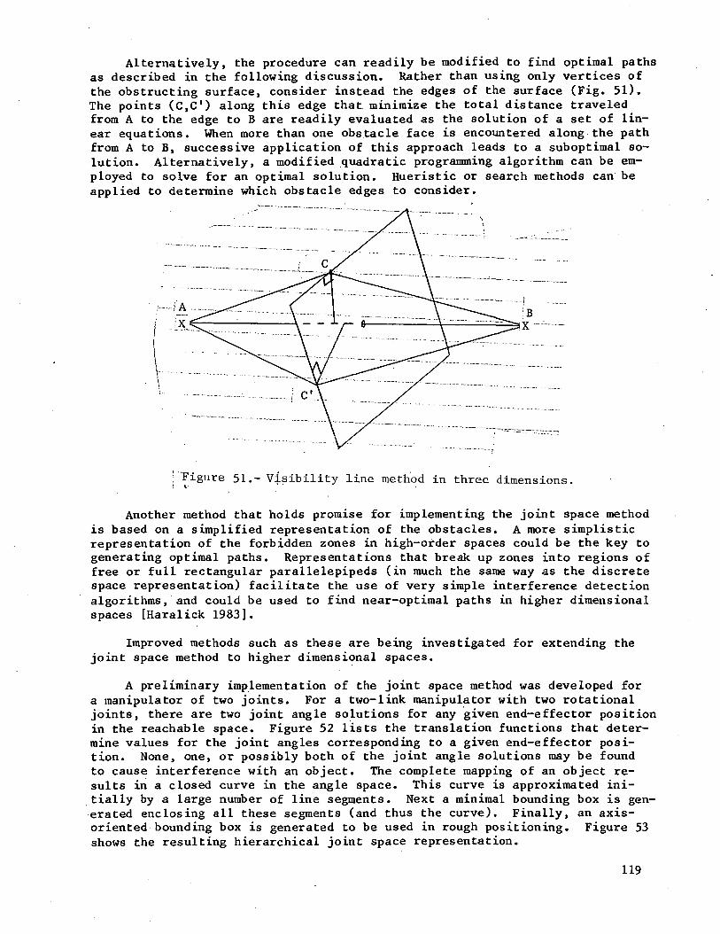
Alternatively, the procedure can readily be modified to find optimal pathsas described in the following discussion. Rather than using only vertices ofthe obstructing surface, consider instead the edges of the surface (Fig. 51).The points (C,C') along this edge that minimize the total distance traveledfrom A to the edge to B are readily evaluated as the solution of a set of lin-ear equations. When more than one obstacle face is encountered along the pathfrom A to B, successive application of this approach leads to a suboptimal so-lution. Alternatively, a modified quadratic programming algorithm can be em-ployed to solve for an optimal solution. Hueristic or search methods can beapplied to determine which obstacle edges to consider.
j "Figure 51.- Visibility line method in three dimensions.
Another method that holds promise for implementing the joint space methodis based on a simplified representation of the obstacles. A more simplisticrepresentation of the forbidden zones in high-order spaces could be the key togenerating optimal paths. Representations that break up zones into regions offree or full rectangular parallelepipeds (in much the same way as the discretespace representation) facilitate the use of very simple interference detectionalgorithms, and could be used to find near-optimal paths in higher dimensionalspaces [Haralick 1983].
Improved methods such as these are being investigated for extending thejoint space method to higher dimensional spaces.
A preliminary implementation of the joint space method was developed fora manipulator of two joints. For a two-link manipulator with two rotationaljoints, there are two joint angle solutions for any given end-effector positionin the reachable space. Figure 52 lists the translation functions that deter-mine values for the joint angles corresponding to a given end-effector posi-tion. None, one, or possibly both of the joint angle solutions may be foundto cause interference with an object. The complete mapping of an object re-sults in a closed curve in the angle space. This curve is approximated ini-tially by a large number of line segments. Next a minimal bounding box is gen-erated enclosing all these segments (and thus the curve). Finally, an axis-oriented bounding box is generated to be used in rough positioning. Figure 53shows the resulting hierarchical joint space representation.
119
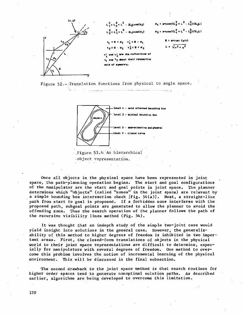
(x.u)
L \ =
L2 -
+ L -
d r KL2. + L2 -
d2 = arccosUL2 # L2 - L| )/2L1LJ
s B - d2
B - dt
8 * d2
t' and t' are the reflections of
t1 and *2 about their respective
axis of suBMtr*.
Figure 52.-^Translation functions from physical to angle space.
level 1 - axis oriented bounding box
level 2 - ninlnal bounding box
level 3 - approxiMting
level 4 - closed curve
.Figure 53.#- An hierarchical
•object representation.
Once all objects in the physical space have been represented in jointspace, the path-planning operation begins. The start and goal configurationsof the manipulator are the start and goal points in joint space. The plannerdetermines which "objects" (called "zones" in the joint space) are relevant bya simple bounding box intersection check [Fig. 54(a)J. Next, a straight-linepath from start to goal is proposed. If a forbidden zone interferes with theproposed path, subgoal points are generated to allow the planner to avoid theoffending zone. Thus the search operation of the planner follows the path ofthe recursive visibility lines method (Fig. 54).
It was thought that an indepth study of the simple two-joint case wouldyield insight into solutions in the general case. However, the generaliz-ability of this method to higher degrees of freedom is inhibited in two impor-tant areas. First, the closed-form translations of objects in the physicalworld to their joint space representations are difficult to determine, espec-ially for manipulators with several degrees of freedom. One method to over-come this problem involves the notion of incremental learning of the physicalenvironment. This will be discussed in the final subsection.
"The second drawback to the joint space method is that search routines forhigher order spaces tend to generate nonoptimal solution paths. As describedearlier, algorithms are being developed to overcome this limitation.
120
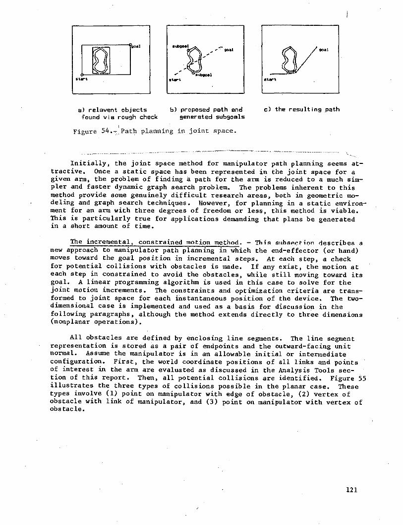
goalSMl goal
evert
a) relavent objectsfound via rouah check
b) proposed path andgenerated subsoals
c) the resulting path
Figure 54.-,Path planning in joint space.
Initially, the joint space method for manipulator path planning seems at-tractive. Once a static space has been represented in the joint space for agiven arm, the problem of finding a path for the arm is reduced to a much sim-pler and faster dynamic graph search problem. The problems inherent to thismethod provide some genuinely difficult research areas, both in geometric mo-deling and graph search techniques. However, for planning in a static environ-ment for an arm with three degrees of freedom or less, this method is viable.This is particularly true for applications demanding that plans be generatedin a short amount of time.
The incremental, constrained motion method. - This subsection describes anew approach to manipulator path planning in which the end-effector (or hand)moves toward the goal position in incremental steps. At each step, a checkfor potential collisions with obstacles is made. If any exist, the motion ateach step in constrained to avoid the obstacles, while still moving toward itsgoal. A linear programming algorithm is used in this case to solve for thejoint motion increments. The constraints and optimization criteria are trans-formed to joint space for each instantaneous position of the device. The two-dimensional case is implemented and used as a basis for discussion in thefollowing paragraphs, although the method extends directly to three dimensions(nonplanar operations).
All obstacles are defined by enclosing line segments. The line segmentrepresentation is stored as a pair of endpoints and the outward-facing unitnormal. Assume the manipulator is in an allowable initial or intermediateconfiguration. First, the world coordinate positions of all links and pointsof interest in the arm are evaluated as discussed in the Analysis Tools sec-tion of this report. Then, all potential collisions are identified. Figure 55illustrates the three types of collisions possible in the planar case. Thesetypes involve (1) point on manipulator with edge of obstacle, (2) vertex ofobstacle with link of manipulator, and (3) point on manipulator with vertex ofobstacle.
121
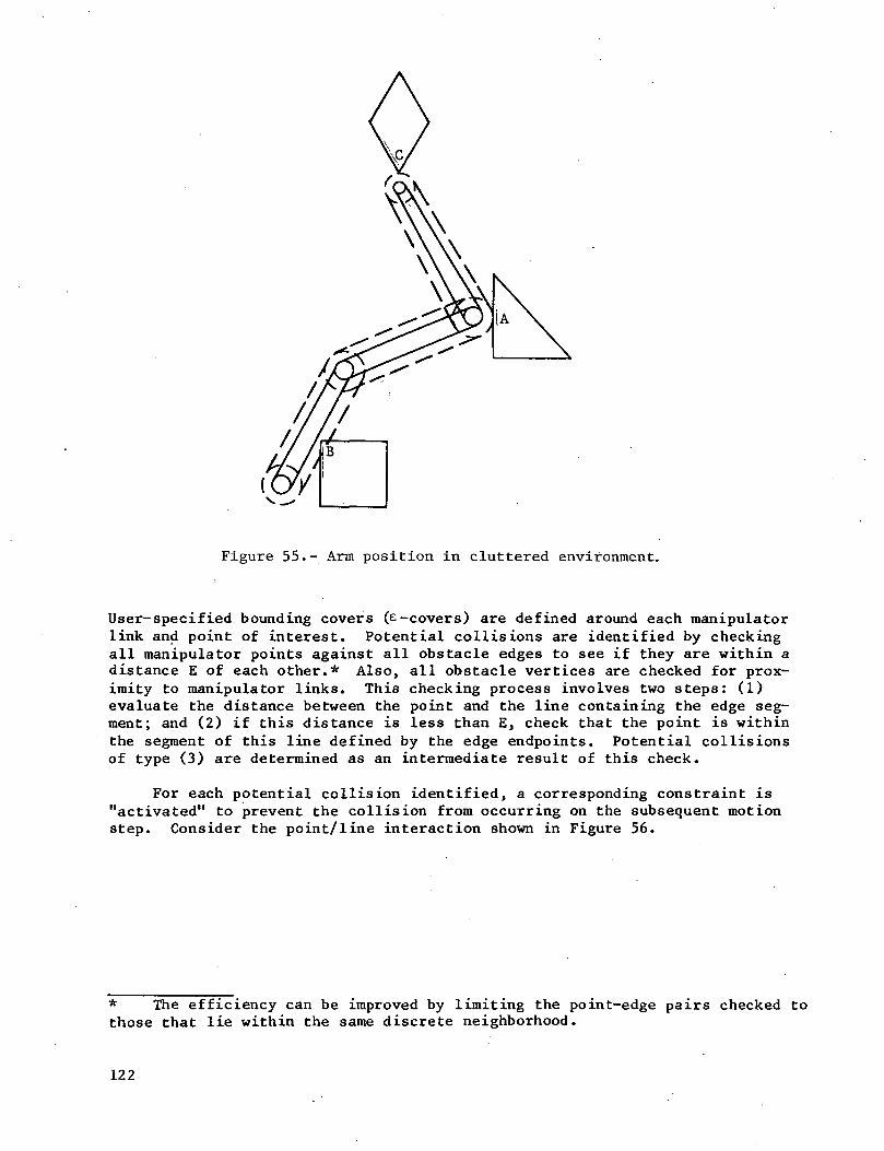
Figure 55.- Arm position in cluttered environment.
User-specified bounding covers (e-covers) are defined around each manipulatorlink and point of interest. Potential collisions are identified by checkingall manipulator points against all obstacle edges to see if they are within adistance E of each other.* Also, all obstacle vertices are checked for prox-imity to manipulator links. This checking process involves two steps: (1)evaluate the distance between the point and the line containing the edge seg-ment; and (2) if this distance is less than E, check that the point is withinthe segment of this line defined by the edge endpoints. Potential collisionsof type (3) are determined as an intermediate result of this check.
For each potential collision identified, a corresponding constraint is"activated" to prevent the collision from occurring on the subsequent motionstep. Consider the point/line interaction shown in Figure 56.
* The efficiency can be improved by limiting the point-edge pairs checked tothose that lie within the same discrete neighborhood.
122
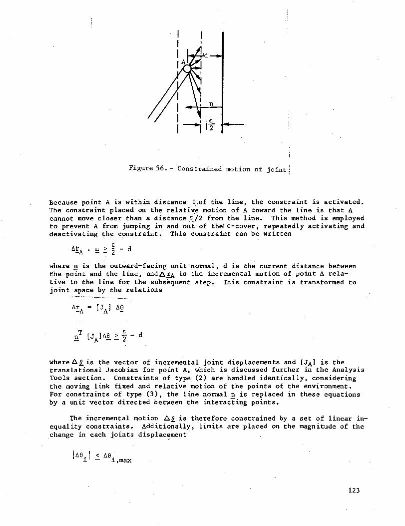
Figure 56. - Constrained motion of joint]
Because point A is within distance '£,of the line, the constraint is activated.The constraint placed on the relative motion of A toward the line is that Acannot move closer than a distanced/2 from the line. This method is employedto prevent A from jumping in and out of the! e-cover, repeatedly activating anddeactivating the constraint. This constraint can be written
A£A • s > i - dwhere n is the outward-facing unit normal, d is the current distance betweenthe point and the line, andA£A *-s t^ie incremental motion of point A rela-tive to the line for the subsequent step. This constraint is transformed tojoint space by the relations
ArA = [JA] AG
where A£ is the vector of incremental joint displacements and [JA] is thetranslational Jacobian for point A, which is discussed further in the AnalysisTools section. Constraints of type (2) are handled identically, consideringthe moving link fixed and relative motion of the points of the environment.For constraints of type (3), the line normal n is replaced in these equationsby a unit vector directed between the interacting points.
The incremental motion A0_ is therefore constrained by a set of linear in-equality constraints. Additionally, limits are placed on the magnitude of thechange in each joints displacement
JA6 | <_ A0.i,max
123
To determine the joint motion stepA'£, an error vector CArl.A n.) pbetween the current hand position and the desired hand position"" is computed asdescribed in a previous section. Then, the equations
are solved, subject to the joint stepsize limits, using the linear equationsolution algorithm previously discussed. This provides straight-line motion ofthe hand toward the goal. If, however, the resulting joint displacements vio-late any of the obstacle-avoidance constraints, the equations are solved by adifferent method.
In this case, all activated joint motion constraints are considered andthe simplex algorithm for linear programming is applied. This is analogous tothe method described for a similar manipulator path-planning problem[Grechanovsky 1981]. The linear optimization criterion is defined by
maximize (Ar • Ar . , + Ad> • Ad> }— p —p, actual -"-p -cp, actual
which Is translated into joint coordinates to give
\ maximize KArJ, A£pT) [Jp] A9>
The joint angles are updated using the resulting vector
and the entire process is recursively repeated until the goal is reached.
Initial testing verified that this algorithm works very well as a low-level planner in an overall planning hierarchy. However, the manipulator caneasily be trapped against the edge of one or more constraints, endlessly cy-cling among a few positions without making any progress toward the goal. Thisproblem illustrates the need for a high-level planner that provides interme-diate goals to the incremental-motion planner and monitors its operation.
The ROBSIM path planner contains an initial implementation of such a highlevel planner. The Cartesian position space of the hand is discretized into afinite number of regions. Weights are assigned to transitions between conti-guous regions; these weights indicate the relative ease of making the hand mo-tion corresponding to that transition (small values indicate the transition isreadily achieved). The high-level planner chooses a goal-directed path, de-fined as a sequence of regions to be traversed, based on these weights. Thecenter point for the next region along the path is specified as the currentgoal for the low-level planner. The high-level planner then monitors the exe-cution of the lower level.
124
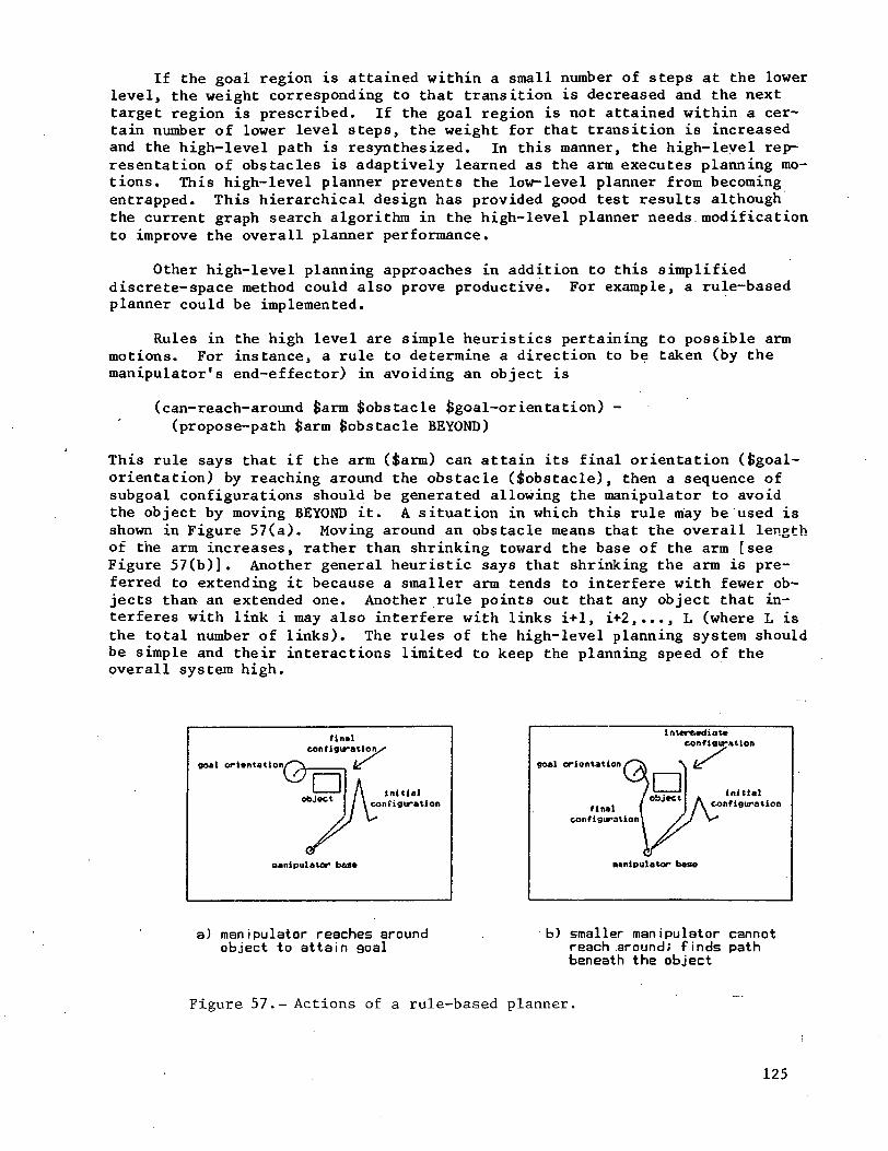
If the goal region is attained within a small number of steps at the lowerlevel, the weight corresponding to that transition is decreased and the nexttarget region is prescribed. If the goal region is not attained within a cer-tain number of lower level steps, the weight for that transition is increasedand the high-level path is resynthesized. In this manner, the high-level rep-resentation of obstacles is adaptively learned as the arm executes planning mo-tions. This high-level planner prevents the low-level planner from becomingentrapped. This hierarchical design has provided good test results althoughthe current graph search algorithm in the high-level planner needs modificationto improve the overall planner performance.
Other high-level planning approaches in addition to this simplifieddiscrete-space method could also prove productive. For example, a rule-basedplanner could be implemented.
Rules in the high level are simple heuristics pertaining to possible armmotions. For instance, a rule to determine a direction to be taken (by themanipulator's end-effector) in avoiding an object is
(can-reach-around fcann obstacle ^goal-orientation) -(propose-path fcarm obstacle BEYOND)
This rule says that if the arm ($arm) can attain its final orientation (fcgoal-orientation) by reaching around the obstacle (^obstacle), then a sequence ofsubgoal configurations should be generated allowing the manipulator to avoidthe object by moving BEYOND it. A situation in which this rule may be used isshown in Figure 57(a). Moving around an obstacle means that the overall lengthof the arm increases, rather than shrinking toward the base of the arm [seeFigure 57(b)] . Another general heuristic says that shrinking the arm is pre-ferred to extending it because a smaller arm tends to interfere with fewer ob-jects than an extended one. Another rule points out that any object that in-terferes with link i may also interfere with links i+1, i+2,..., L (where L isthe total number of links). The rules of the high-level planning system shouldbe simple and their interactions limited to keep the planning speed of theoverall system high.
finalconfiguration^
goal orientation
initialconfiguration
oanipulator bas*
goal orientation
intcnwdiateconfiguration
initialfinal \ °bJ*"i A configuration
configuration)
K•anipulator base
a) manipulator reaches aroundobject to attain goal
b) smaller manipulator cannotreach around; finds pathbeneath the object
Figure 57.- Actions of a rule-based planner.
125
The high-level planner does not attempt to find complete collision-freepaths in any sense. Rather, it guides the operation of the low-level plannerusing information about the current state of the manipulator to generate plaus-ible paths. This system may attempt ultimately impossible paths for some timebefore deciding on a new approach. However, when this happens, the system canbe capable of large "jumps" back to previous manipulator configurations, par-ticularly if the planning is completed before the motion begins. This back-tracking scheme is maintained by the high-level system. Thus, when an attemptto reach a goal orientation becomes less desirable (or fails) in the currentpath direction than in some previous one, the system may return attention tothe previous path, possibly jumping back over many attained configurations.
Comparison of Current Methods and Directions for Further Study
Three methods stand out as viable solutions to the problem of manipulatorpath planning—the generalized cone representation of free space, modeling phy-sical environments in joint space, and incremental, constrained-motion plan-ning. Each of these methods is directly applicable to manipulator path-planning problems. However, depending on the application, one method may bemore suitable than another. In this section, each of these methods is dis-cussed in terms of its strengths and weaknesses in various path-planning do-mains. Following this is a brief discussion of directions for further study.
The generalized cone representation of free space. - Recall that repre-senting physical environments as a set of intersecting generalized cones in-volves finding cones between relatively facing edges (or faces, in three dimen-sions) of all the objects in the environment. The time required to generatethe representation grows rapidly with the number of objects.* For this reason,the method is limited to applications involving only sparsely populated envir-onments. However, if objects may be represented in terms of simple geometricfigures (such as bounding boxes or rectangular parallelepipeds), evaluation ofthe free space becomes more efficient.
Another limitation of this approach is that solutions are determined sole-ly through examination of possible freeway paths. This leads to the same pro-blem as the discretizing of an environment; namely, the algorithm may not finda path even when one exists. This is because the object moving through the en-vironment must remain aligned on a freeway at all times. Additionally, rota-tion is allowed only at freeway intersections (i.e., within the intersection oftwo cones). Thus, the planner may fail to find paths that require rotation be-tween two intersection points. If the distance between objects in the environ-ment is relatively large in comparison with the size of a manipulator's links,this is only a minor problem.
* According to Brooks, the algorithm has complexity (n3) "n cubed" in num-ber of objects for 2D worlds; (n4) "n to the fourth" for 3D (see [Brooks1983a], pps. 194, 196).
126
Modeling physical environments in joint space. - The most limiting aspectof this approach is calculation of the joint space representation of the physi-cal world. Because there are many ways for a real manipulator to attain agiven end-effector position, an £ priori determination of all possible arm in-terferences is difficult, if not impossible. However, a preliminary determina-tion involving the first three of a manipulator's joints (base, shoulder, andelbow) may be made, providing an approximation of free space suitable for rougharm positioning. This approach alone is viable in applications involving man-ipulators with three degrees of freedom or less, or those that do not requireaccurate arm positioning.
A combination joint space/linear programming approach would be viable inapplications requiring accurate positioning of manipulators with more thanthree joints. Using this approach, the low-level linear optimization plannerdiscussed would be coupled with a high-level planner that initially has no in-formation regarding the physical environment. It would incrementally "learn"a joint space approximation of the environment as the low-level planner movedabout and detected obstacles. This amounts to "feeling around" blindly in thephysical world, with the advantage of remembering every position. In a clut-tered environment, this system would initially find awkward paths. However, asthe manipulator moved about more and more, the high-level planner would developan accurate representation of the joint space that would be used to guide thearm along collis ion-free paths. This combination approach provides a means ofmodeling the joint space that avoids the complexity of a priori calculation.This adaptive, hierarchical path-planning algorithm could also accommodatechang ing env i ronmen t s.
The incremental, constrained-motion method. - This planning method is verypromising, especially when coupled with an intelligent high-level planner thatgenerates subgoals for the motion. No restriction as to the size of the envir-onment or the number of components it may contain is imposed, nor is the systemrestricted to finding paths of a certain type. The number of degrees of free-dom of arm motions is not limited and multiple arm systems can be accommodated.Sensor information can readily be incorporated in the description of the systemand environment. Thus, this planner is especially well-suited for operation insituations where knowledge regarding the free space in an environment is eithertoo costly to calculate or is impossible to determine ahead of time. This ap-plies in either extremely cluttered static worlds or in dynamic environments.
Directions for further study. - Complex manipulator path planning in astatic environment may be successfully accomplished using any of the threemethods previously discussed. However, in any real world application of ro-botics technology, a manipulator will be expected to attain very accurate posi-tions many times during a given task (e.g., inspection, assembly, or machineoperation). Time constraints may also be imposed on the operation of the en-tire robotic system. These two characteristics require that a path plannergenerate plans in a very short amount of time. Some marriage between existingmethods will be necessary to accomplish this. For example, the generalizedcone method is capable of fast rough arm positioning in a simplified represen-tation of an environment. The incremental, constrained-motion planner is cap-able of fine positioning in complex environments. Coupled with the adaptivelearning of joint space, such a system could operate very well, especially instatic environments. The system could switch back and forth between the twoplanning methods, using the generalized cone approach for large moves through
127
uncluttered regions of the environment and the bilevel incremental planningsystem for smaller moves requiring finer positioning. The two operations couldbe done in parallel so by the time a plan to attain a rough configuration wascompleted, a path from there to the actual goal configuration would also havebeen generated. Such a planning system is being developed at Martin MariettaDenver Aerospace.
The main assumption of all present path-planning methods has been that theenvironment to be operated on does not change. For most real-world applica-tions, this is an invalid assumption. Many applications, such as assembly, re-quire the manipulator to move objects around in the environment. This is knownas a dynamic application. The path planner may be constructed under the safeassumption that the system will be aware of all objects in its environment.The only constraint relaxed is that the obstacles remain stationary.*
This class of path-planning problems becomes even more complex when ob-jects other than the manipulator may be in motion. For example, severalmanipulators may be working together in intersecting workspaces. The onlytechnique suggested thus far for path planning in this situation is to allowonly one arm to be in motion at a time whenever one is inside the working en-velope of another. This amounts to assuming a static configuration for one (ormore) arms while generating a path for another and forcing the former to assumethat configuration and stop while the latter moves. One advantage of the in-cremental, constrained-motion method is that it can readily be extended to ac-commodate interacting arms, simultaneously controlling the manipulators toavoid each other.
One direction for path-planning research that would allow for less con-strained operation in the case just described is toward execution of partialplans. This method is also viable in simpler applications with time-criticalplanning constraints. Several issues to be resolved include when .to begin exe-cution, physical "backtracking" of the manipulator when the current route isfound to be impossible, and communication among path planners for the variousmoving bodies.
* There are two subclasses of this type of environment, one in which objectsare moved only by the manipulator, and one in which objects may be moved byother means.
128
IMAGE PROCESSING AND VIDEO SIMULATION
A video simulation software module was developed to simulate the output ofa video camera mounted on or near a simulated manipulator. A ROBSIM graphicsrepresentation depicting a scene of a PUMA 600 manipulator in a peg-in-the-holescenario was generated with the ROBSIM program. Conversion of these data to aform used by the MOVIE.BYU package available on the Ramtek raster graphics de-vice was performed. The single scene was then displayed using shaded graphicsand color with the MOVIE.BYU package to generate a raster image of the scene;this image was then used as input to various edge detection algorithm modules.This method of ROBSIM geometry database conversion to MOVIE.BYU format may beused to generate a raster image of any ROBSIM scene on which new image process-ing algorithms, such as the edge detection and thresholding operations ex-plained here, may be performed to enhance the resulting picture.
Edge Detection
An edge in a digital image is a change in intensities. However, an imagecontains many intensity changes, not all of which represent physical edges.For example, consider an image of a cube illuminated by a nearby point source*Intensity changes in the image occur at the intersection of two faces becauseof the change in the angle of reflection, and along each face because of thechange in distance from the light source. In this example, a computer visionsystem must be able to distinguish the intensity changes caused by physicaledges from those caused by other factors.
Edge detection schemes generally involve three stages of processing:
1) Edge pixels are detected;
2) Edge pixels are thinned to eliminate all but significant edges;
3) Edge points are linked to form lines, curves, etc.
Each of these stages is discussed in the following sections.
Detecting edge pixels. - Consider an image as a three-dimensional surfacewhere each intensity value denotes the height of the surface at that point.Then changes in intensity represent changes in surface height, and the magni-tude of an intensity change represents the magnitude of the surface slope.Hence, one approach to identifying the "edgeness" of a pixel is to treat theimage as a surface and compute the magnitude of the surface slope at eachpixel. On a continuous surface, this computation would involve computing thedirectional derivatives at each point. Because a digital image is a discretefunction, difference operators are used to approximate the derivatives.
129
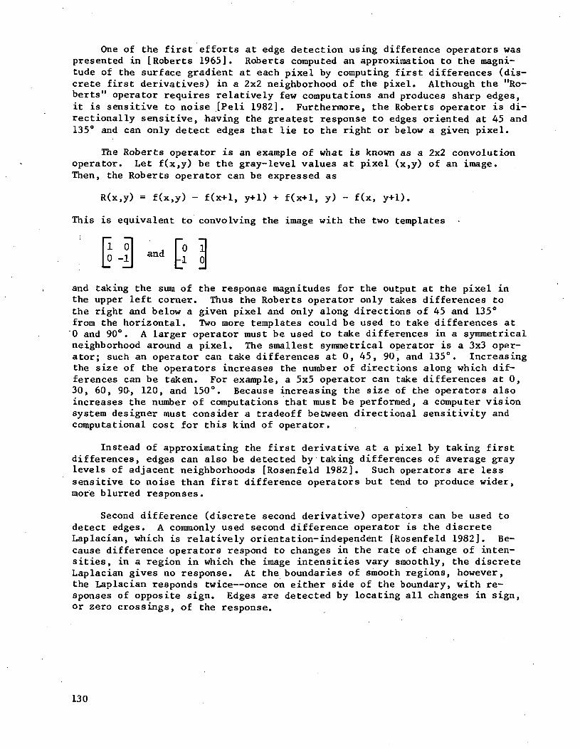
One of the first efforts at edge detection using difference operators waspresented in [Roberts 1965]. Roberts computed an approximation to the magni-tude of the surface gradient at each pixel by computing first differences (dis-crete first derivatives) in a 2x2 neighborhood of the pixel. Although the "Ro-berts" operator requires relatively few computations and produces sharp edges,it is sensitive to noise [Peli 1982], Furthermore, the Roberts operator is di-rectionally sensitive, having the greatest response to edges oriented at 45 and135° and can only detect edges that lie to the right or below a given pixel.
The Roberts operator is an example of what is known as a 2x2 convolutionoperator. Let f(x,y) be the gray-level values at pixel (x,y) of an image.Then, the Roberts operator can be expressed as
R(x,y) = f(x,y) - f(x+l, y+1) + f(x+l, y) - f(x, y+1).
This is equivalent to convolving the image with the two templates
1 °1 , FO 1° 41 and b Iand taking the sum of the response magnitudes for the output at the pixel inthe upper left corner. Thus the Roberts operator only takes differences tothe right and below a given pixel and only along directions of 45 and 135°from the horizontal. Two more templates could be used to take differences at0 and 90°. A larger operator must be used to take differences in a symmetricalneighborhood around a pixel. The smallest symmetrical operator is a 3x3 oper-ator; such an operator can take differences at 0, 45, 90, and 135°. Increasingthe size of the operators increases the number of directions along which dif-ferences can be taken. For example, a 5x5 operator can take differences at 0,30, 60, 90-, 120, and 150°. Because increasing the size of the operators alsoincreases the number of computations that must be performed, a computer visionsystem designer must consider a tradeoff between directional sensitivity andcomputational cost for this kind of operator.
Instead of approximating the first derivative at a pixel by taking firstdifferences, edges can also be detected by taking differences of average graylevels of adjacent neighborhoods [Rosenfeld 1982]. Such operators are lesssensitive to noise than first difference operators but tend to produce wider,more blurred responses.
Second difference (discrete second derivative) operators can be used todetect edges. A commonly used second difference operator is the discreteLaplacian, which is relatively orientation-independent [Rosenfeld 1982]. Be-cause difference operators respond to changes in the rate of change of inten-sities, in a region in which the image intensities vary smoothly, the discreteLaplacian gives no response. At the boundaries of smooth regions, however,the Laplacian responds twice—once on either side of the boundary, with re-sponses of opposite sign. Edges are detected by locating all changes in sign,or zero crossings, of the response.
130
[Binford 1981] noted that a distinction should be made between the pro-cesses of detecting edges and localizing edges. A first difference operatorperforms well at detecting edges but responds over a broad region and is there-fore poor for localizing edges. A second difference operator, however, per-forms well at the localization task but is more sensitive to noise [Rosenfeld1982]. [MacVicar-Whelan 1981] reports edge localization to subpixel accuracyusing a second difference operator.
[Prewitt 1970] first introduced a method for detecting edges by using thegradient of the best-fit polynomial surface in the neighborhood of a pixel.Using a least squares criterion, a polynomial surface is fit to a symmetricneighborhood around each pixel in an image. The magnitude of the gradient ofthe best-fit surface is used as the measure of the edgeness of each pixel. Thesize of the templates used is determined by the order of the polynomial surfaceto be fit. For example, a 3x3 Prewitt operator computes the gradient magnitudeof the best-fit plane at each pixel, whereas a 5x5 operator uses the best-fitquadratic surface.
Edge detection can also be performed by fitting an ideal step edge to theneighborhood of a point. Generally, this technique is implemented using basisfunctions. The neighborhood of a pixel is expanded in terms of some orthogonalbasis, and the coefficients of the expansion are compared with those for theexpansion of an ideal step edge. By adjusting the coefficients of the idealedge to minimize the squared differences between the sets of coefficients, thebest-fit step edge through each pixel can be determined. [Hueckel 1971] wasthe first to use this technique by expanding regions in terms of the Fourierbasis functions. [O'Gorman 1978] used Walsh functions. [Hummel 1977] used theKarhunen-Loeve expansion to derive a set of basis functions that are optimalfor the detection of step edges. [Morgenthaler 1981] combined the techniquesof surface fitting and step edge fitting to propose an edge detector using alocal model of a step edge superimposed on a polynomial surface.
Thinning edge pixels. - The fact was pointed out earlier that one of thedifficulties in edge detection is detecting only the significant edges out ofall the edges present in an image. This section discusses some of the ap-proaches that have been developed for thinning out the edges in an attempt toleave only the significant edges.
Decision-theoretic concepts can be used to thin edges [Rosenfeld 1982]).Suppose that a finite number of regions can be formed in an image, and supposethat the probabilities of a pixel being in each region or on a bor-der are known. Then, if the probability densities of the edge detector re-sponses in the regions or borders can be estimated, the probability of a givenpixel being an edge can be computed.
The magnitude of the response of a first difference operator is propor-tional to the size of the intensity change at a point. If the assumption ismade that large intensity changes are significant, one approach to thinningfirst difference operators is to threshold the edge picture at a particularedge strength, retaining only the edge pixels at which edge strength exceedsthe threshold. However, this thinning technique fails if the strength of sig-nificant edges varies greatly over an image. For example, consider an image ofobjects in partial shadow. Object edges in shadow are faint and are likely tobe lost if a global threshold is used. [Rosenfeld 1971] suggested suppressing
131
all edges except the strongest for some distance taken perpendicular to theedge. [Hanson 1980] used local thresholding based on the distribution of edgestrengths in square local neighborhoods.
[Rosenfeld 1971] also proposed a multistep technique for determining the"best" edge at a point. The technique requires taking the differences of aver-ages using neighborhoods of many different sizes. Each of the resulting edgepictures is thinned by suppressing nonmaxima across the edge. Finally, a com-posite edge picture is obtained by comparing the different edge strengths ob-tained at each pixel. Let e'*1' (i,j) be the edge strength (after initialthinning) at pixel (i,j) using a difference of averages operator of size hxh.The final edge strength at (i,j) is given by e'm' (i,j) where m is the lar-gest value such that
. ..e
but
The symbol "< " is taken to mean "much smaller than," and in the initial im-plementation of Rosenfeld and Thurston, meant roughly "less than three-quartersof." This algorithm is capable of detecting texture edges and was shown in[Peli 1982] to be fairly tolerant of noise.
Smoothing an image before applying an edge detector can reduce the effectsof noise. Many kinds of smoothing operators exist and are discussed in textson image processing (see, for example, [Rosenfeld 1982]). Operators can be de-signed that combine the operations of smoothing and edge detection.
[Binford 1981] proposed that a particular technique be implemented tosmooth a picture for edge detection. He calls the technique "lateral inhibi-tion." Implementation consists of subtracting from each pixel value the aver-age intensity of the eight pixels immediately surrounding it. The lateral in-hibition operation effectively suppresses the effects of smooth variations inintensity.
[Shanmugan 1979] proposed a frequency domain filter for edge detection.The proposed filter yields a maximum response in the vicinity of an edge. Forthe special case of a step edge, the optimal frequency domain filter is thesecond derivative of a Gaussian. Marr and Hildreth [Marr 1980] proposed anedge detector using the convolution of a.Gaussian smoothing function with aLaplacian. The Marr-Hildreth edge detector employs operators of several dif-ferent sizes to detect edges at various resolutions [Hildreth 1982].
132
The Marr-Hildreth edge detector produces good results but is computa-tionally expensive; the templates used are huge by conventional standards—thesmallest is 32x32 pixels [Brady 1982]. However, improvements in computerhardware technology may make even such large operators feasible for use inreal-time applications. Nishihara and Larson designed a special-purpose pro-cessor for performing convolutions [Nishihara 1981]. The processor is capableof convolving a 1000x1000 image with the smallest Marr-Hildreth operator inabout 1 second [Hildreth 1982]. Even greater speed can be expected as thestate of the art in hardware improves.
Linking edge pixels. - After detection and thinning of edges have beenperformed, the next step is to link edges together to impose some order on theimage. The ways in which edge pixels are linked depend on the kinds of linearfeatures expected to be in an image.
Rosenfeld and Thurston [Rosenfeld 1971] proposed algorithms for detectingthin curves and wide streaks. Using their formulation, a point lies on a thincurve if it satisfies two conditions:
"Condition 1: It has a pair of lower valued neighbors on opposite sides ofit (in the direction across the curve).Condition 2: It has two other neighbors (in the direction along the curvethat satisfy Condition 1."
Variations of this algorithm can be used to link pixels belonging to a varietyof linear features.
[Shirai 1978] used gradient magnitude and direction, as well as a classi-fication of edge type to link edges. The edge types used are shown in Figure58. Linking proceeds in two stages. First, edge "kernels" or sets of pixelsof the same type and direction, are identified. Then, each kernel is extendedby tracking as far as possible in both directions. Tracking consists of pre-dicting the position and gradient values of the next point, and adding pixelsto the edge if their values differ from those predicted within prespecifiedtolerances. Predictions are updated every time a pixel is added, enabling thetechniques to track curved edges as well as straight ones.
Ballard and Brown [Ballard 1982] advocated the use of the Hough transformto detect arbitrary curves. As an explanation of the technique, consider theexample of detecting straight lines (following the development of Ballard andBrown). Let (x,y) be an edge pixel in an image. Any line through (x,y) isgiven by the equation y = mx + c. Because the set of all possible linesthrough (x,y) is represented by a line in m,c-space, each edge pixel in an im-age can be associated by a line in m,c-space; the set of edge pixels then cor-responds to a set of lines in m,c-space. If two edge pixels lie on the sameline in an image, their corresponding lines will intersect in m,c-space.Therefore, a straight line in an image will be represented as the intersectionof many lines in m,c-space. By detecting clusters in m,c-space, lines in animage can be detected. The Hough transform technique can be extended to detectany kind of parameterized feature.
133
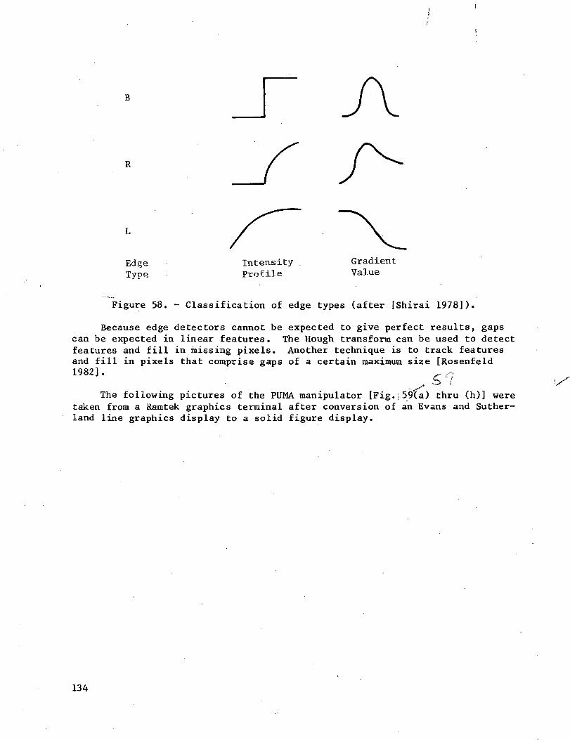
R
EdgeType
Intensity .Profile
GradientValue
Figure 58. - Classification of edge types (after [Shirai 1978]).
Because edge detectors cannot be expected to give perfect results, gapscan be expected in linear features. The Hough transform can be used to detectfeatures and fill in missing pixels. Another technique is to track featuresand fill in pixels that comprise gaps of a certain maximum size [Rosenfeld1982]. . s-,
. 6" /- «•'•'
The following pictures of the PUMA manipulator [Fig.;59(a) thru (h)] weretaken from a Ramtek graphics terminal after conversion of an Evans and Suther-land line graphics display to a solid figure display.
134

"Page missing from available version"
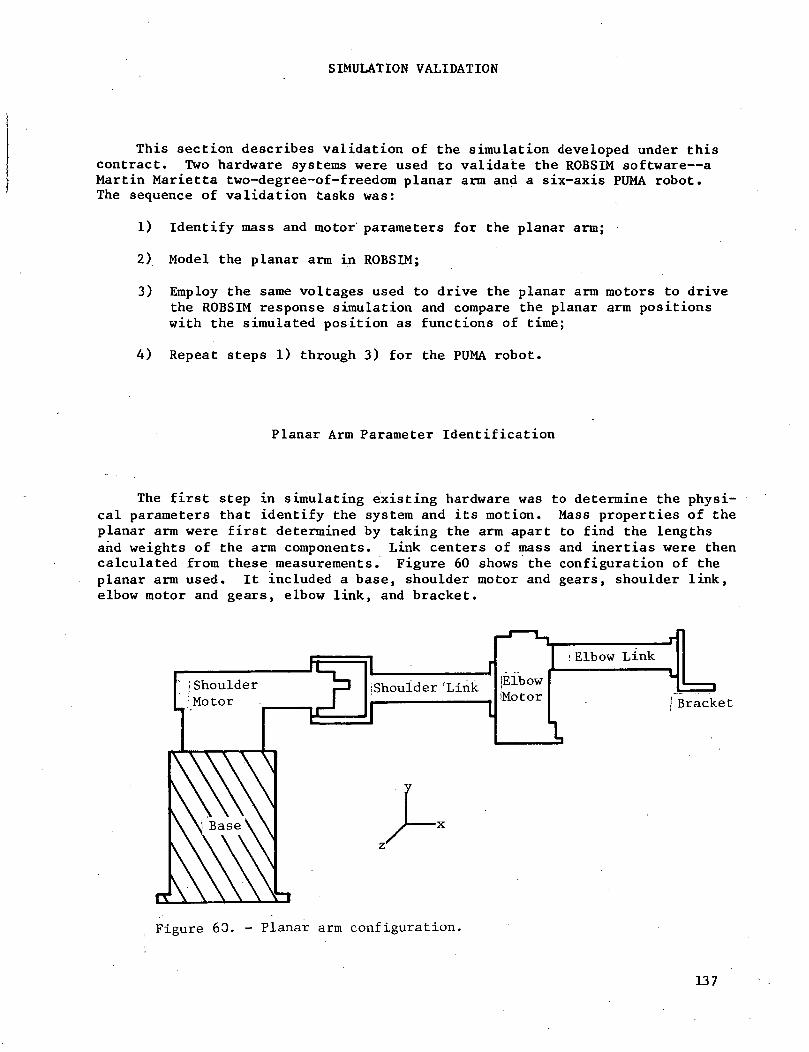
SIMULATION VALIDATION
This section describes validation of the simulation developed under thiscontract. Two hardware systems were used to validate the ROBSIM software—aMartin Marietta two-degree-of-freedom planar arm and a six-axis PUMA robot.The sequence of validation tasks was:
1) Identify mass and motor parameters for the planar arm;
2) Model the planar arm in ROBSIM;
3) Employ the same voltages used to drive the planar arm motors to drivethe ROBSIM response simulation and compare the planar arm positionswith the simulated position as functions of time;
4) Repeat steps 1) through 3) for the PUMA robot.
Planar Arm Parameter Identification
The first step in simulating existing hardware was to determine the physi-cal parameters that identify the system and its motion. Mass properties of theplanar arm were first determined by taking the arm apart to find the lengthsand weights of the arm components. Link centers of mass and inertias were thencalculated from these measurements. Figure 60 shows the configuration of theplanar arm used. It included a base, shoulder motor and gears, shoulder link,elbow motor and gears, elbow link, and bracket.
fip- 1F I Shoulder ID
; Motor . |i I H"
1 i(Shoulder 'Link
J I
jElbowiMotor
: Elbow Linki
j
1I Bracket
Figure 60. - Planar arm configuration.
137
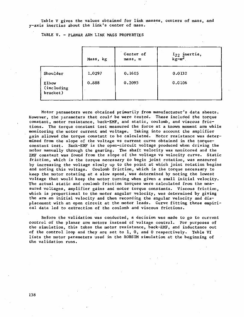
Table V gives the values obtained for link masses, centers of mass, andy-axis inertias about the link's center of mass.
TABLE V. - PLANAR ARM LINK MASS PROPERTIES
Mass, kgCenter ofmass, m
122 inertia,kg-ra2.
Shoulder
Elbow(includingbracket)
1.0297
0.888
0.1605
0.2095
0.0132
0.0106
Motor parameters were obtained primarily from manufacturer's data sheets.However, the parameters that could be were tested. These included the torqueconstant, motor resistance, back-EMF, and static, coulomb, and viscous fric-tions. The torque constant test measured the force at a known moment arm whilemonitoring the motor current and voltage. Taking into account the amplifiergain allowed the torque constant to be calculated. Motor resistance was deter-mined from the slope of the voltage vs current curve obtained in the torque-constant test. Back-EMF is the open-circuit voltage produced when driving themotor manually through the gearing. The shaft velocity was monitored and theEMF constant was found from the slope of the voltage vs velocity curve. Staticfriction, which is the torque necessary to begin joint rotation, was measuredby increasing the voltage slowly up to the point at which joint rotation beginsand noting this voltage. Coulomb friction, which is the torque necessary tokeep the motor rotating at a slow speed, was determined by noting the lowestvoltage that would keep the motor turning when given a small initial velocity.The actual static and coulomb friction torques were calculated from the mea-sured voltages, amplifier gains and motor torque constants. Viscous friction,which is proportional to the motor angular velocity, was determined by givingthe arm an initial velocity and then recording the angular velocity and dis-placement with an open circuit at the motor leads. Curve fitting these empiri-cal data led to extraction of the coulomb and viscous frictions.
Before the validation was conducted, a decision was made to go to currentcontrol of the planar arm motors instead of voltage control. For purposes ofthe simulation, this takes the motor resistance, back-EMF, and inductance outof the control loop and they are set to 1, 0, and 0 respectively. Table VIlists the motor parameters used in the ROBSIM simulation at the beginning ofthe validation runs.
138
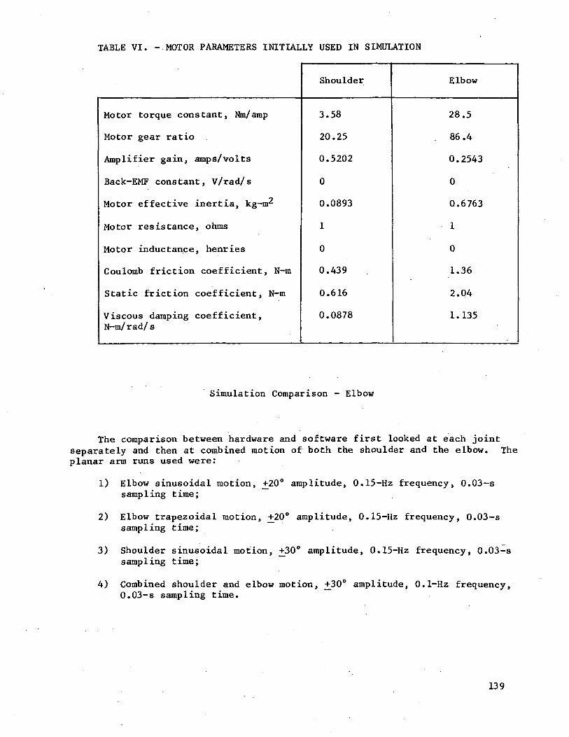
TABLE VI. - MOTOR PARAMETERS INITIALLY USED IN SIMULATION
Motor torque constant, Nm/arap
Motor gear ratio
Amplifier gain, amps/ volts
Back-EMF constant, V/rad/s
Motor effective inertia, kg-m^
Motor resistance, ohms
Motor inductance, henries
Coulomb friction coefficient, N-m
Static friction coefficient, N-m
Viscous damping coefficient,N-m/rad/s
Shoulder
3.58
20.25
0.5202
0
0.0893
1
0
0.439
0.616
0.0878
Elbow
28.5
. 86.4
0 . 2543
0
0.6763
1
0
1.36
2.04
1.135
Simulation Comparison - Elbow
The comparison between hardware and software first looked at each jointseparately and then at combined motion of both the shoulder and the elbow. Theplanar arm runs used were:
1) Elbow sinusoidal motion, 20° amplitude, 0.15-Hz frequency, 0.03-ssampling time;
2) Elbow trapezoidal motion, ±20° amplitude, 0.15-Hz frequency, 0.03-ssampling time;
3) Shoulder sinusoidal motion, +30° amplitude, 0.15-Hz frequency, 0.03-ssampling time;
4) Combined shoulder and elbow motion, ;+30° amplitude, 0.1-Hz frequency,0.03-s sampling time.
139
The simulation modeled the planar arm using the parameters in Tables V andVI. Response simulation runs were executed in ROBSIM using the same controlvoltage used to control the planar arm. To compare the motion of the simula-tion with that of the actual hardware arm, one of the ROBSIM postprocessing op-tions was used. This option plays back the motion that occurred during ananalysis run, and also simultaneously displays a stick figure whose motions re-present the motion of the hardware arm.
The first hardware motion to be simulated was the sinusoidal elbow motion.Although the first attempt showed agreement in the direction of motion, thesimulation amplitude and accelerations were too large. To attempt to obtainbetter agreement, the elbow motor torque constant and friction coefficientswere reevaluated. The torque constant was determined by attaching the force/torque wrist to the arm and then increasing the voltage to the elbow motor andmeasuring the force exerted against a constraint. The slope of the force volt-age curve multiplied by the amplifier gain and moment arm defined the motortorque constant. This testing obtained a torque constant of 12.8 Nra/amp forthe elbow motor. The static friction torque was obtained by increasing thevoltage to the elbow joint until the joint moved. This voltage was then multi-plied by the amplifier gain and motor torque constant. The coulomb frictiontorque was evaluated by changing the voltage to find the lowest voltage thatwould keep the joint moving after it was given a small initial velocity. Mul-tiplying by the amplifier gain and torque constant gave the actual frictiontorque value. This static friction torque was also evaluated by looking at theplanar arm motor voltage and position plots. The voltage at which motion be-gins (at extreme reach of each cycle) was used to calculate the static frictiontorque. The coulomb friction torque is approximately two-thirds of the statictorque. Testing the arm gave values of 1.5 Nra and 1.0 Nm for static and cou-lomb friction respectively. The voltage taken from the plot indicated staticfriction to be about 2.4 Nm. In testing both sets of values in the simulation,it was noted that the higher friction values seemed to give better agreementwith the hardware positions. At this point the agreement between the hardwareand the simulation was quite good. Both reached the .same amplitude and wouldstart motion in the new direction at the same time. However, the simulationwould move out more quickly and reach the end of the motion and stop before thehardware would. This seemed to indicate that the effective inertia of thejoint/link pair was too low. Because it was assumed that the link inertia wasaccurately known, it was assumed that the motor effective inertia was in error.The elbow motor inertia was increased until the motion of the hardware andsimulation matched well. This meant increasing the inertia from 0.68 to 1.8.The positions of the elbow of the planar arm and its simulation are shown inFigure^61. (In the figure h denotes the hardware motion and s the simulation.)The negative shift of the simulation was because the arm was probably not ex-actly in the horizontal plane so gravity caused the motor drive voltage to beslightly greater in one direction than the other.
After the sinusoidal motion was matched, the voltages used for trapezoidalmotion of the planar arm elbow were used to control a response simulation runof ROBSIM. Figure 62 shows the hardware and simulation elbow positions fortrapezoidal motion.
140
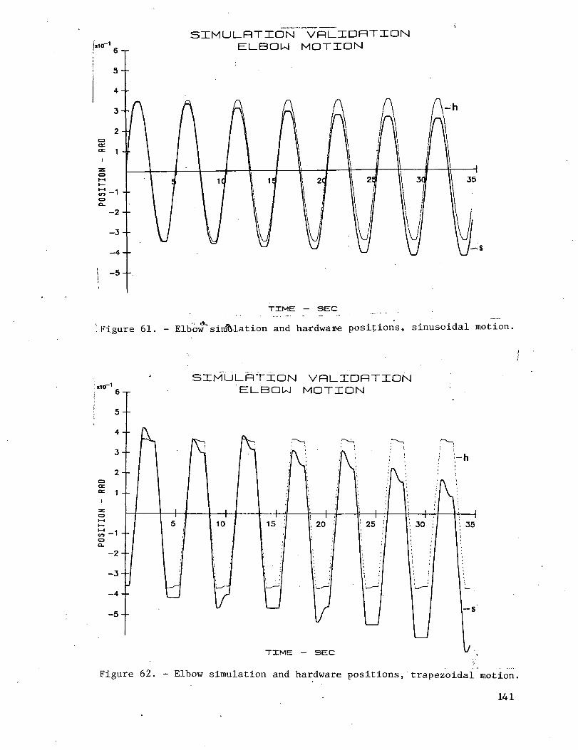
ixlO"
SIMULRTION VRLIDRTIONELBOW MOTION
TIME — SEC
-h
!Figure 61. - Elbow"simulation and hardware positions, sinusoidal motion.
ST-MUL-RTILON VRLIDRTIONELBOW MOTION
-h
TIME - SEC
Figure 62. - Elbow simulation and hardware positions, trapezoidal motion.
141
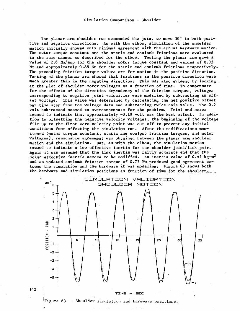
Simulation Comparison - Shoulder
The planar arm shoulder run commanded the joint to move 30° in both posi-tive and negative directions. As with the elbow, simulation of the shouldermotion initially showed only minimal agreement with the actual hardware motion.The motor torque constant and the static and coulomb frictions were evaluatedin the same manner as described for the elbow. Testing the planar arm gave avalue of 2.6 Mm/amp for the shoulder motor torque constant and values of 0.95Nm and approximately 0.88 Nm for the static and coulomb frictions respectively.The preceding friction torque values are for motion in the positive direction.Testing of the planar arm showed that frictions in the positive direction weremuch greater than in the negative direction. This was also evident by lookingat the plot of shoulder motor voltages as a function of time. To compensatefor the effects of the direction dependency of the friction torques, voltagescorresponding to negative joint velocities were modified by subtracting an off-set voltage. This value was determined by calculating the net positive offsetper time step from the voltage data and subtracting twice this value. The 0.2volt subtracted seemed to overcompensate for the problem. Trial and errorseemed to indicate that approximately -0.18 volt was the best offset. In addi-tion to offsetting the negative velocity voltages, the beginning of the voltagefile up to the first zero velocity point was cut off to prevent any initialconditions from affecting the simulation run. After the modifications men-tioned (motor torque constant, static and coulomb friction torques, and motorvoltages), reasonable agreement was obtained between the planar arm shouldermotion and the simulation. But, as with the elbow, the simulation motionseemed to indicate a low effective inertia for the shoulder joint/link pair.Again it was assumed that the link inertia was fairly accurate and that thejoint effective inertia needed to be modified. An inertia value of 0.45 kg-m^and an updated coulomb friction torque of 0.77 Nm produced good agreement be-tween the simulation and the hardware it was modeling. Figure 63 shows boththe hardware and simulation positions as function of time for the shquj.der.
xicr1
6-r
SZEMULRTION VRL.IDRTZONSHOULDER MOTHION
142\ TIME - SEC
iFigure 63. - Shoulder simulation and hardware positions.
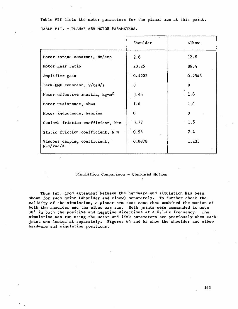
Table VII lists the motor parameters for the planar arm at this point.
TABLE VII. - PLANAR ARM MOTOR PARAMETERS.
Motor torque constant, Mm/ amp
Motor gear ratio
Amplifier gain
Back-EMF constant, V/rad/s
Motor effective inertia, kg-iar
Motor resistance, ohms
Motor inductance, henries
Coulomb friction coefficient, N-m
Static friction coefficient, N-m
Viscous damping coefficient,N-m/rad/s
Shoulder
2.6
20.25
0.5202
0
0.45
1.0
0
0.77
' 0.95
0.0878
Elbow
12.8
86.4
0.2543
0
' 1.8
1.0
0
1.5
2.4
1.135
Simulation Comparison - Combined Motion
Thus far, good agreement between the hardware and simulation has beenshown for each joint (shoulder and elbow) separately. To further check thevalidity of the simulation, a planar arm test case that combined the motion ofboth the shoulder and the elbow was run. Both joints were commanded to move30° in both the positive and negative directions at a 0.1-Hz frequency. Thesimulation was run using the motor and link parameters set previously when eachjoint was looked at separately. Figures 64 and 65 show the shoulder and elbowhardware and simulation positions.
143
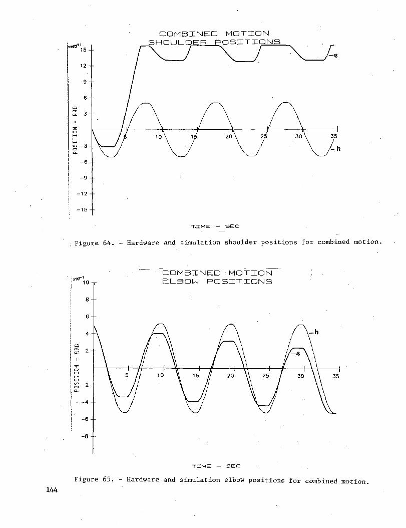
xKJTS*
COMBINED MOTIONSHOULDER POSITIONS,.
T.ICME - SEC
Figure 64. - Hardware and simulation shoulder positions for combined motion.
COMBINED MOTIONELBOW POSITIONS
-h
144
TIME — SEC
Figure 65. - Hardware and simulation elbow positions for combined motion.
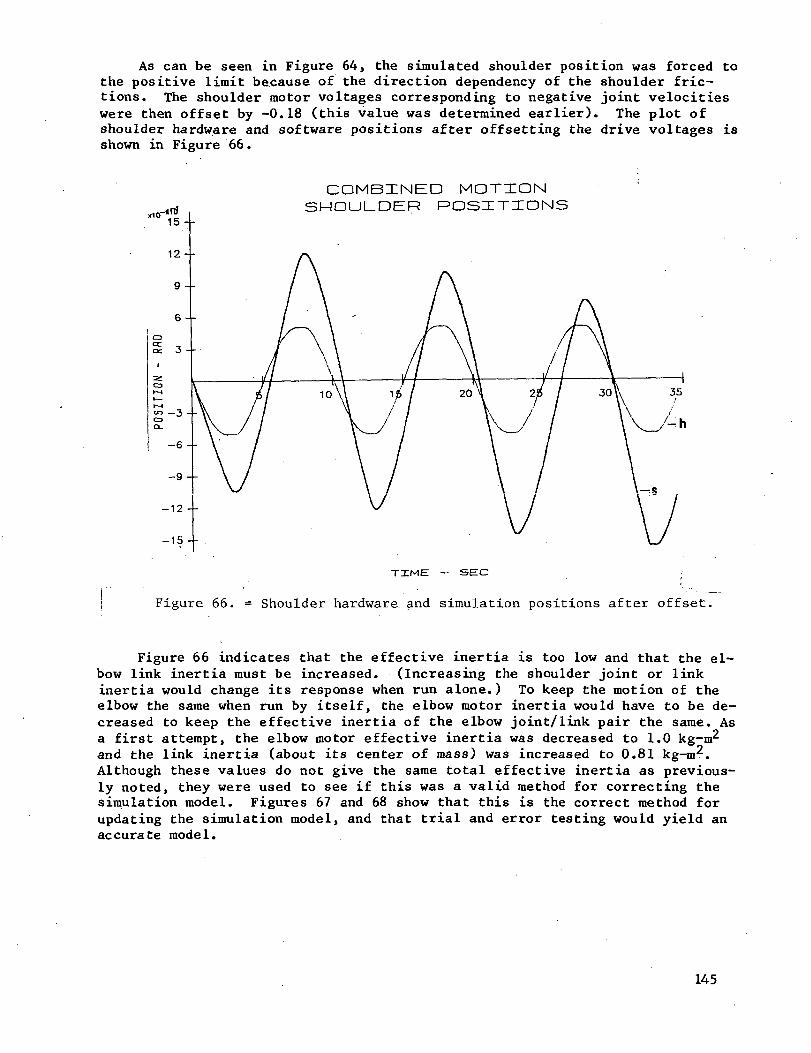
As can be seen in Figure 64, the simulated shoulder position was forced tothe positive limit because of the direction dependency of the shoulder fric-tions. The shoulder motor voltages corresponding to negative joint velocitieswere then offset by -0.18 (this value was determined earlier). The plot ofshoulder hardware and software positions after offsetting the drive voltages isshown in Figure 66.
COMBINED MOTIONSHOULDER POSITIONS
x10~
/-h
-15 --
TIME — SEC
Figure 66. = Shoulder hardware and simulation positions after offset.
Figure 66 indicates that the effective inertia is too low and that the el-bow link inertia must be increased. (Increasing the shoulder joint or linkinertia would change its response when run alone.) To keep the motion of theelbow the same when run by itself, the elbow motor inertia would have to be de-creased to keep the effective inertia of the elbow joint/link pair the same. Asa first attempt, the elbow motor effective inertia was decreased to 1.0 kg-m^and the link inertia (about its center of mass) was increased to 0.81 kg-m^.Although these values do not give the same total effective inertia as previous-ly noted, they were used to see if this was a valid method for correcting thesimulation model. Figures 67 and 68 show that this is the correct method forupdating the simulation model, and that trial and error testing would yield anaccurate model.
145
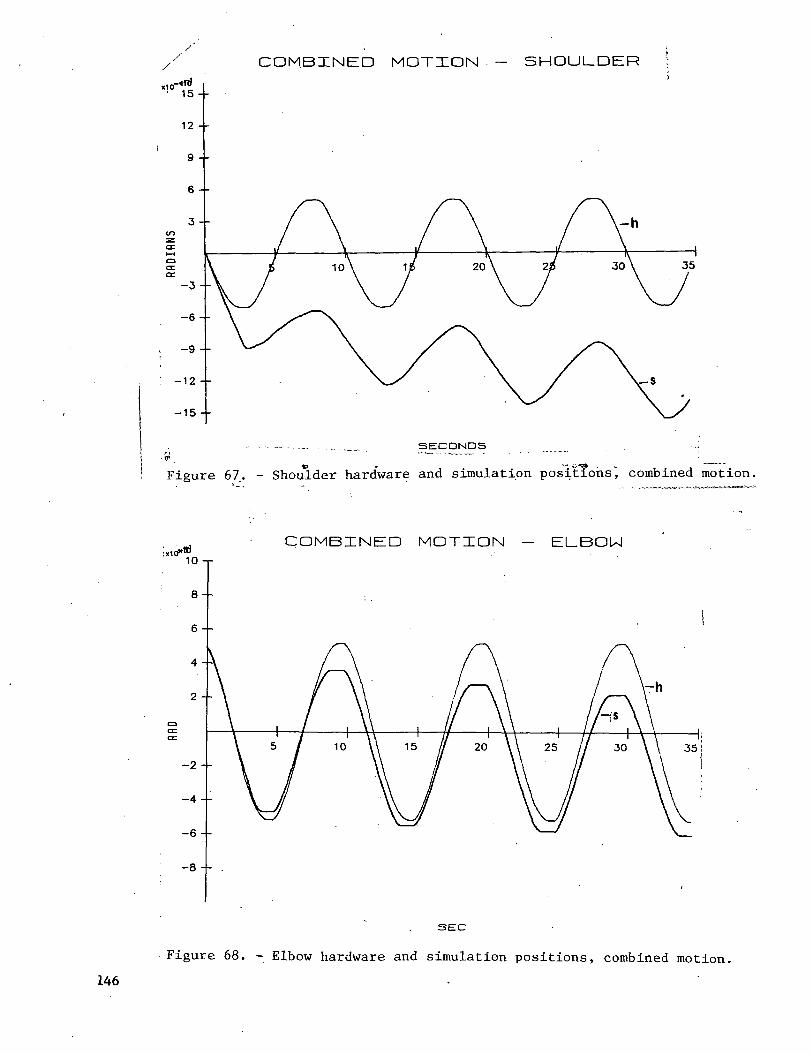
COM.BINED MOTION - SHOULDER
SECONDS
Figure 67. - Shoulder hardware and simulation positions", combined motion.
COMBINED MOTION - ELBOU
SEC
Figure 68. - Elbow hardware and simulation positions, combined motion.
146
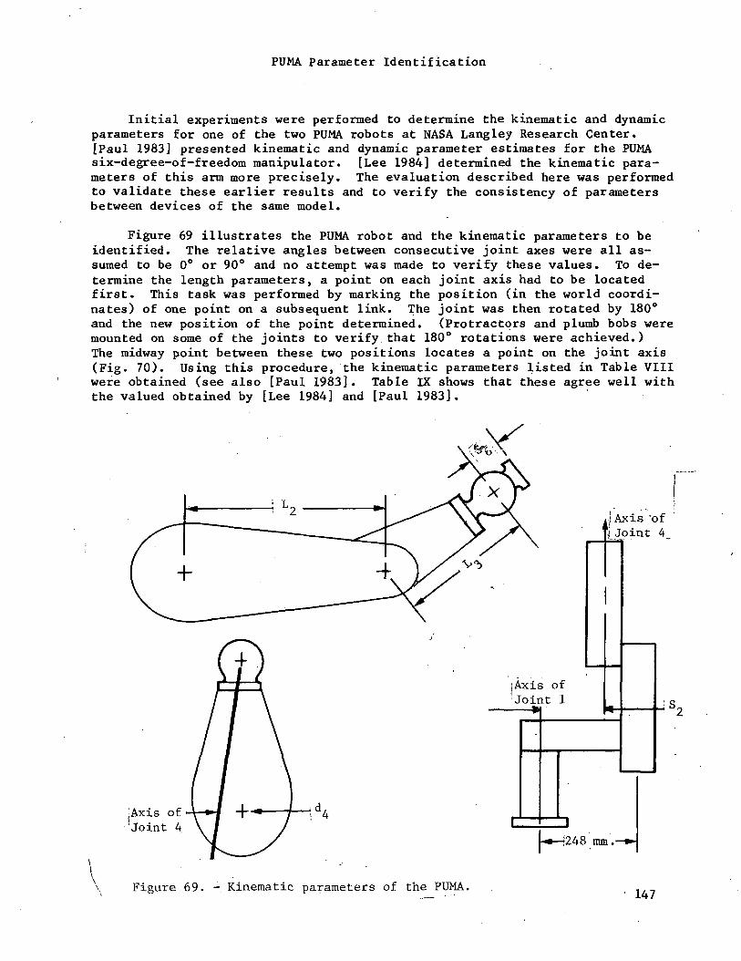
PUMA Parameter Identification
Initial experiments were performed to determine the kinematic and dynamicparameters for one of the two PUMA robots at NASA Langley Research Center.[Paul 1983] presented kinematic and dynamic parameter estimates for the PUMAsix-degree-of-freedom manipulator. [Lee 1984] determined the kinematic para-meters of this arm more precisely. The evaluation described here was performedto validate these earlier results and to verify the consistency of parametersbetween devices of the same model.
Figure 69 illustrates the PUMA robot and the kinematic parameters to beidentified. The relative angles between consecutive joint axes were all as-sumed to be 0° or 90° and no attempt was made to verify these values. To de-termine the length parameters, a point on each joint axis had to be locatedfirst. This task was performed by marking the position (in the world coordi-nates) of one point on a subsequent link. The joint was then rotated by 180°and the new position of the point determined. (Protractors and plumb bobs weremounted on some of the joints to verify that 180° rotations were achieved.)The midway point between these two positions locates a point on the joint axis(Fig. 70). Using this procedure, the kinematic parameters listed in Table VIIIwere obtained (see also [Paul 1983]. Table IX shows that these agree well withthe valued obtained by [Lee 1984] and [Paul 1983].
jAxis of -'Joint 4
Axis "of'I Joint 4_A
iAxis of* Joint 1 J.S,
HJ248 mm.-
Figure 69. - Kinematic parameters of the PUMA.147
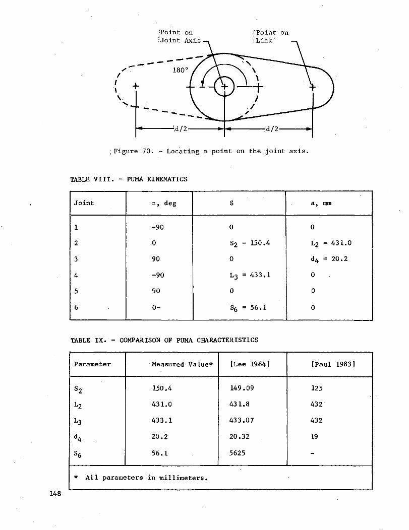
/
V
jPoint on[Joint Axis
180
4d/2
! Point oni Link
Figure 70. - Locating a point on the joint axis.
TABLE VIII. - PUMA KINEMATICS
Joint
1
2
3
4
5
6
a, deg
-90
0
90
-90
90
0-
S
0
S2 = 150.4
0
L3 = 433.1
0
S6 = 56.1
a, mm
0
L2 = 431.0
d4 = 20.2
0
0
0
TABLE IX. - COMPARISON OF PUMA CHARACTERISTICS
Parameter
s2
L2
^3
d4
S6
Measured Value*
150.4
431.0
433.1
20.2
56.1
[Lee 1984]
149.09
431.8
433.07
20.32
5625
[Paul 1983]
125
432
432
19
-
* All parameters in millimeters.
148
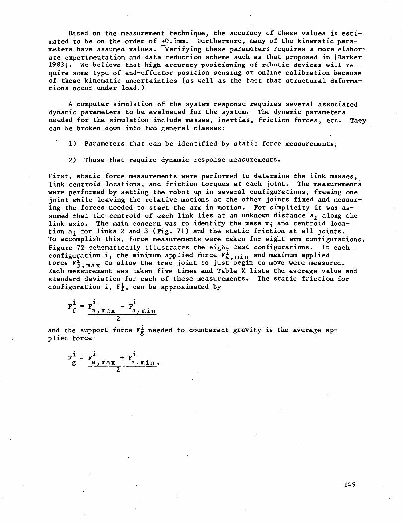
Based on the measurement technique, the accuracy of these values is esti-mated to be on the order of jf0.5mm. Furthermore, many of the kinematic para-meters have assumed values. Verifying these parameters requires a more elabor-ate experimentation and data reduction scheme such as that proposed in [Barker1983]. We believe that high-accuracy positioning of robotic devices will re-quire some type of end-effector position sensing or online calibration becauseof these kinematic uncertainties (as well as the fact that structural deforma-tions occur under load.)
A computer simulation of the system response requires several associateddynamic parameters to be evaluated for the system. The dynamic parametersneeded for the simulation include masses, inertias, friction forces, etc. Theycan be broken down into two general classes:
1) Parameters that can be identified by static force measurements;
2) Those that require dynamic response measurements.
First, static force measurements were performed to determine the link masses,link centroid locations, and friction torques at each joint. The measurementswere performed by setting the robot up in several configurations, freeing onejoint while leaving the relative motions at the other joints fixed and measur-ing the forces needed to start the arm in motion. For simplicity it was as-sumed that the centroid of each link lies at an unknown distance a^ along thelink axis. The main concern was to identify the mass m£ and centroid loca-tion a^ for links 2 and 3 (Fig. 71) and the static friction at all joints.To accomplish this, force measurements were taken for eight arm configurations.Figure 72 schematically illustrates the eight test configurations. In eachconfiguration i, the minimum applied force Fajltiin and maximum appliedforce F* max
to aH°w tne free joint to just begin to move were measured.Each measurement was taken five times and Table X lists the average value andstandard deviation.for each of these measurements. The static friction forconfiguration i, Fj, can be approximated by
PJ - F1 - F1 .f a , max a, mm2
and the support force Fi needed to counteract gravity is the average ap-plied force
F1 = F1 + F1 .g a , max a , mm .
149
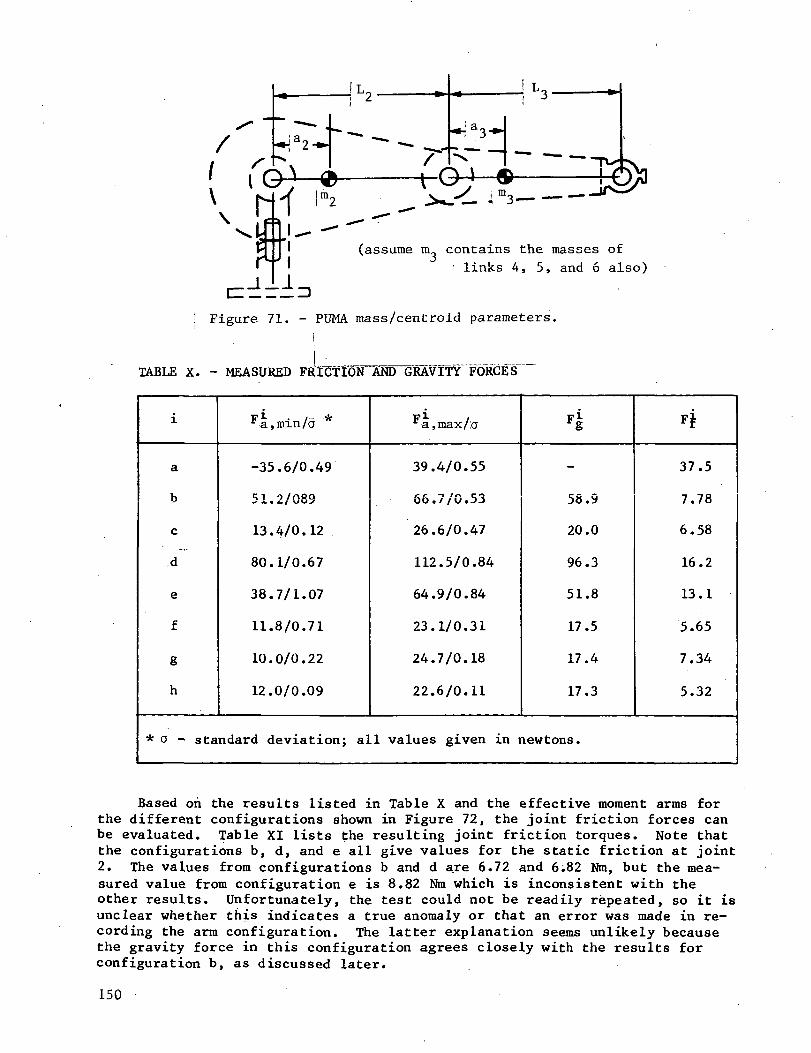
(assume m. contains the masses of1 links 4, 5, and 6 also)
Figure 71. - PUMA mass/centroid parameters.
TABLE X. - MEASURED FRICTION AND GRAVITYFORCES'
i
a
b
c
d
e
f
g
h
Fl,min/o *
-35.6/0.49
51.2/089
13.4/0.12
80.1/0.67
38.7/1.07
11.8/0.71
10.0/0.22
12.0/0.09
Fi ia,max/;a
39.4/0.55
66. 7/0. 53
26.6/0.47
112.5/0.84
64.9/0.84
23.1/0.31
24.7/0.18
22.6/0.11
Fl
-
58.9
20.0
96.3
51.8
17.5
17.4
17.3
4
37.5
7.78
6.58
16.2
13.1
5.65
7.34
5.32
* a - standard deviation; all values given in newtons.
Based oh the results listed in Table X and the effective moment arms forthe different configurations shown in Figure 72, the joint friction forces canbe evaluated. Table XI lists the resulting joint friction torques. Note thatthe configurations b, d, and e all give values for the static friction at joint2. The values from configurations b and d are 6.72 and 6;82 Nm, but the mea-sured value from configuration e is 8.82 Nm which is inconsistent with theother results. Unfortunately, the test could not be readily repeated, so it isunclear whether this indicates a true anomaly or that an error was made in re-cording the arm configuration. The latter explanation seems unlikely becausethe gravity force in this configuration agrees closely with the results forconfiguration b, as discussed later.
150
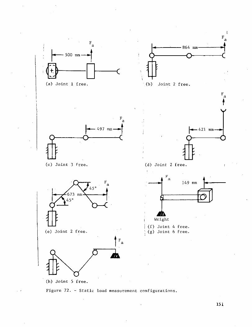
U 500 mm M
(a) Joint 1 free.
£ffl
864 mm-
-O—
(b) Joint 2 free.
oL— 497 mm_*J
o -<
(c) Joint 3 free.
tV
^ 421 mm
O
(d) Joint 2 free.
(e) Joint 2 free.
149 mm k*-
a
[ Weight
! (f) Joint 4 free.! (g) Joint 6 free.
(h) Joint 5 free.
Figure 72. - Static load measurement configurations.
151
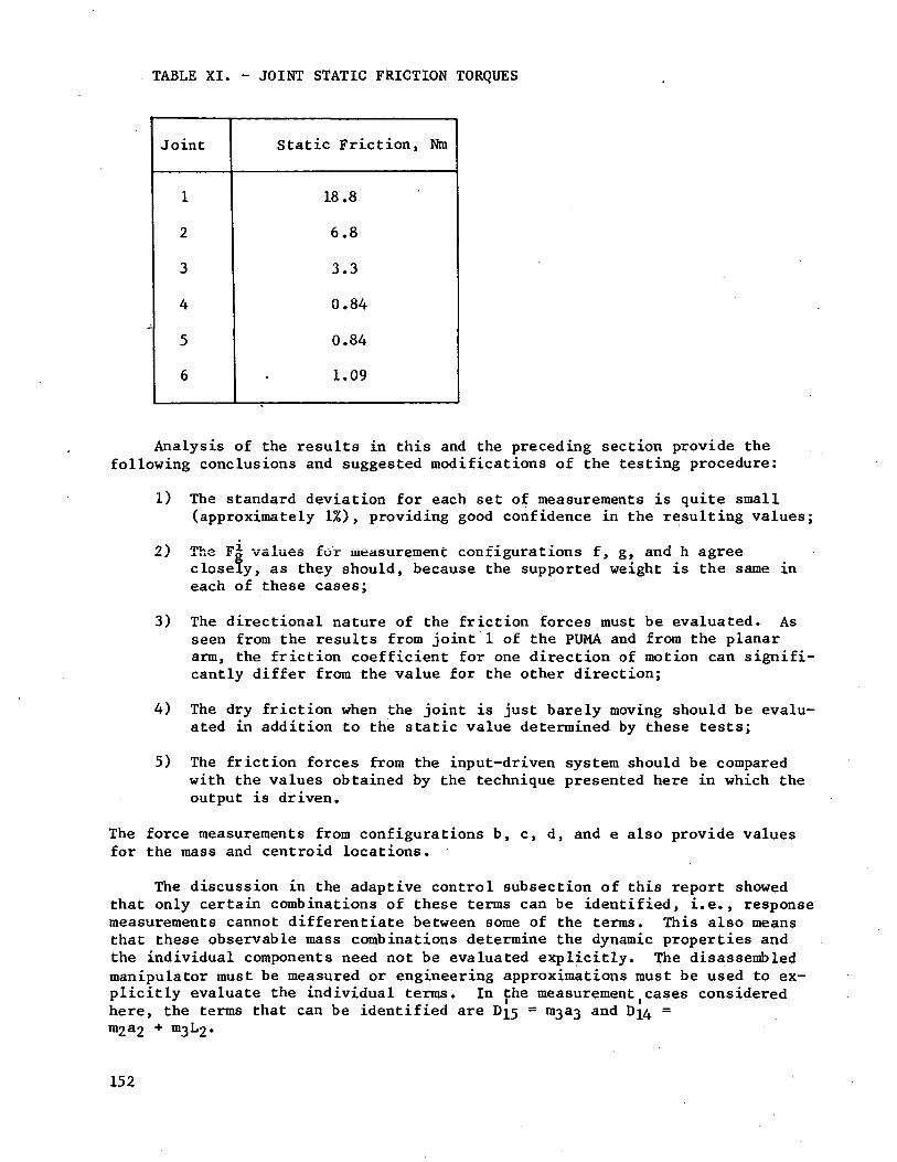
TABLE XI. - JOINT STATIC FRICTION TORQUES
Joint
1
2
3
4
5
6
Static Friction, Nm
18.8
6.8
3.3
0.84
0.84
1.09
Analysis of the results in this and the preceding section provide thefollowing conclusions and suggested modifications of the testing procedure:
1) The standard deviation for each set of measurements is quite small(approximately 1%), providing good confidence in the resulting values;
2) The Fg values for measurement configurations f, g, and h agreeclosely, as they should, because the supported weight is the same ineach of these cases;
3) The directional nature of the friction forces must be evaluated. Asseen from the results from joint 1 of the PUMA and from the planararm, the friction coefficient for one direction of motion can signifi-cantly differ from the value for the other direction;
4) The dry friction when the joint is just barely moving should be evalu-ated in addition to the static value determined by these tests;
5) The friction forces from the input-driven system should be comparedwith the values obtained by the technique presented here in which theoutput is driven.
The force measurements from configurations b, c,for the mass and centroid locations.
d, and e also provide values
The discussion in the adaptive control subsection of this report showedthat only certain combinations of these terms can be identified, i.e., responsemeasurements cannot differentiate between some of the terras. This also meansthat these observable mass combinations determine the dynamic properties andthe individual components need not be evaluated explicitly. The disassembledmanipulator must be measured or engineering approximations must be used to ex-plicitly evaluate the individual terms. In the measurement cases consideredhere, the terms that can be identified are D]^ = 111333 and 0^4 =
152
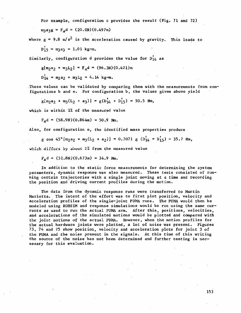
For example, configuration c provides the result (Fig. 71 and 72)
m3a3g = Fad = (20. ON) (0.497m)
where g = 9.8 m/s^ is the acceleration caused by gravity. This leads to
Di5 = 111333 = 1.01 kg-m,
Similarly, configuration d provides the value for D^4 as
g[m2a2 + m3L2] = Fad = (96.3N)(0.421)m
= m2a2 + m3L2 = 4.14 kg-m.
.These values can be validated by comparing them with the measurements from con-figurations b and e. For configuration b, the values given above yield
g[m2a2 + m3(L2 + 33)] = g(D 4 + D^) = 50.5 Nm,
which is within 1% of the measured value
Fad = (58.9N)(0.864m) = 50.9 Nra.
Also, for configuration e, the identified mass properties produce
g cos 45°[m2a2 + m3(L2 + a2)] = 0.7071 g (Dj . = D^) = 35.7 Nm,
which differs by about 2% from the measured value
Fad = (51.8N)(0.673m) = 34.9 Nm.
In addition to the static force measurements for determining the systemparameters, dynamic response was also measured. These tests consisted of run-ning certain trajectories with a single joint moving at a time and recordingthe position and driving current profiles during the motion.
The data from the dynamic response runs were transferred to MartinMarietta. The intent of the effort was to first plot position, velocity andacceleration profiles of the single-joint PUMA runs. The PUMA would then bemodeled using ROBSIM and response simulations would be run using the same cur-rents as used to run the actual PUMA arm. After this, positions, velocities,and accelerations of the simulated motions would be plotted and compared withthe joint motions of the actual PUMA. However, when the motion profiles forthe actual hardware joints were plotted, a lot of noise was present. Figures73, 74 and 75 show position, velocity and acceleration plots for joint 3 ofthe PUMA and the noise present in the signals. At this time of this writingthe source of the noise has not been determined and further testing is nec-essary for this evaluation.
153
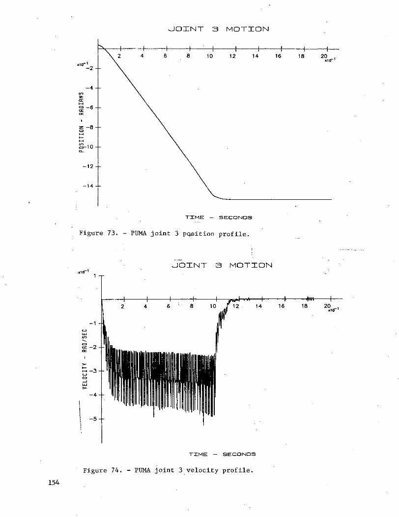
UOINT 3 MOTION
x10~
-14 --
TIME - SECONDS
Figure 73. - PUMA joint 3 position profile.
JOINT 3 MOTION
12 14 16 18
TIME - SECONDS
Figure 74. - PUMA joint 3 velocity profile.
154
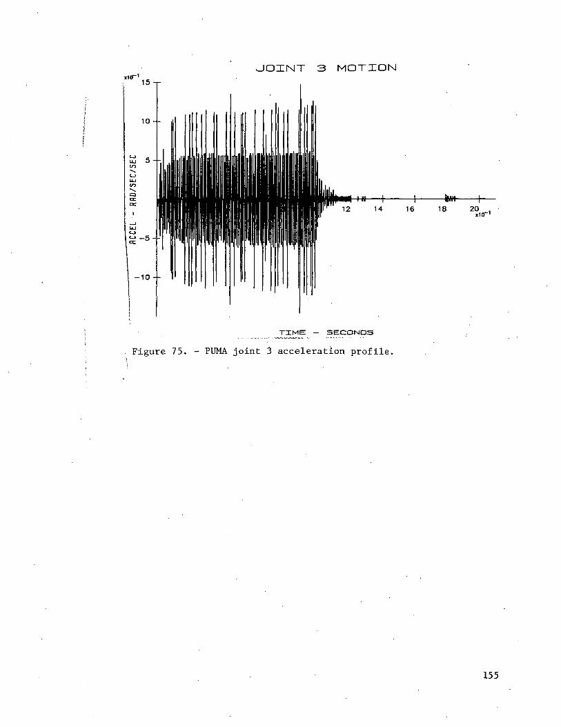
JOINT 3 MOTION
16 18 20
TIME - SECONDS
Figure 75. - PUMA joint 3 acceleration profile.
155
CONCLUDING REMARKS
This report has documented the work done in Phases II and HI of contractNASl-16759, Evaluation of Automated Decisionmaking Methodologies and Develop-ment of an Integrated Robotic System Simulation. The tasks defined for PhaseII (tasks 9 thru 13) and Phase III (14 thru 20) have significantly increasedthe capabilities of the robotic simulation (ROBSIM) package and the technolo-gies associated with the automation and operation of advanced manipulator sys-tems listed:
1) System definition - The implementation of this module allows a user todefine a manipulator system consisting of multiple arms, load objectsand an environment. This addressed task 12 of the contract;
2) Analysis capabilities - This has added the capabilities of kinematicanalysis, requirements analysis, and response simulation for investi-gating manipulator motion. This addressesed tasks 14, 15, and 16;
3) Postprocessing - This module allows the user to better evaluate sys-tem analysis results through the graphic replay of simulated motionor manipulator parameter plots;
4) Control - Various control methods were investigated and those imple-mented in ROBSIM include manual force/torque and active compliancecontrol. This addressed tasks 13, 17 and 19 of the contract;
5) Trajectory planning - Three methods of obstacle avoidance were imple-mented and evaluated and research was conducted in the field of tra-jectory planning. This work addressed tasks 9 and 18;
6) Image processing - The module implemented video simulation and edgedetection and addressed tasks 10 and 11;
7) Simulation validation - The software simulation was validated in con-junction with the Automation Technology Branch of NASA-LRC. This workaddresses task 20 of the contract.
Target areas for future enhancement of the ROBSIM capabilities includegreater ease of user interaction with the program, expanded manipulator model-ing abilities, and the addition of system compliance in the model.
Expansion of the ROBSIM software could now be directed toward support ofteleoperator and robotic systems capable of such remote space operations as theremote orbital servicing system (ROSS) concept. The simulation could supportdual manipulator arms attached to a carrier spacecraft in orbit. Forces, mo-ments and motions typical of a dual-arm robot/host vehicle system of this typewould be included in the kinematic and dynamic solutions. It is anticipatedthat the models for the manipulator motors, the sensors and end-effector willwarrant the development of new software modules and laboratory validation ex-periments. Figure 76 is a sample of a preliminary ROSS simulation graphicsdisplay.
156
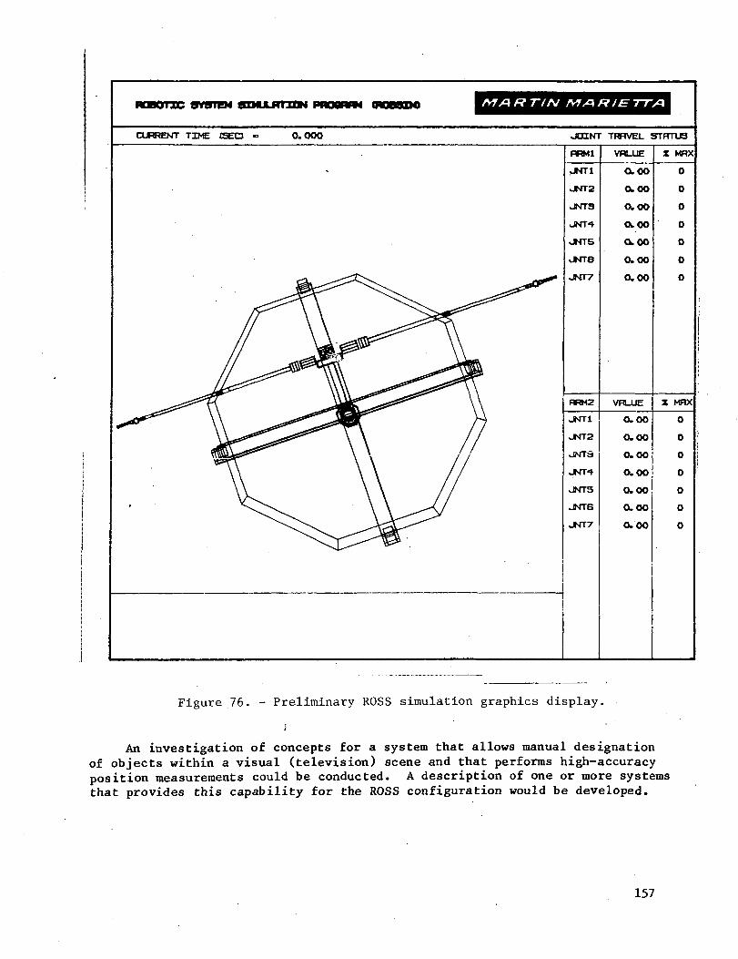
ATXJ f=f TIN A?X» Ft IE TTA
OXRtNT TIKE CSEO O.OOO JOINT TRRVEL STfTTUS
PRM1
.JNT1
JNT2
JNT3
JNT4
JNT5
JNT8
JNT7
RRM2
JNT1
JNT2
JNTS
JNT4
JNT5
JNT6
JNT7
VflLUE
O.OO
OwOO
O.OO
0.00O.OO
O.OO
O.OO
VFB-UE
O.OO
OwOO
O.OO
O.OO
O.OO
O.OO
O.OO
Z MPX
o0
o0
0
oo
X MRX
o0
0
o0
0
0
Figure 76. - Preliminary ROSS simulation graphics display.
An investigation of concepts for a system that allows manual designationof objects within a visual (television) scene and that performs high-accuracyposition measurements could be conducted. A description of one or more systemsthat provides this capability for the ROSS configuration would be developed.
157
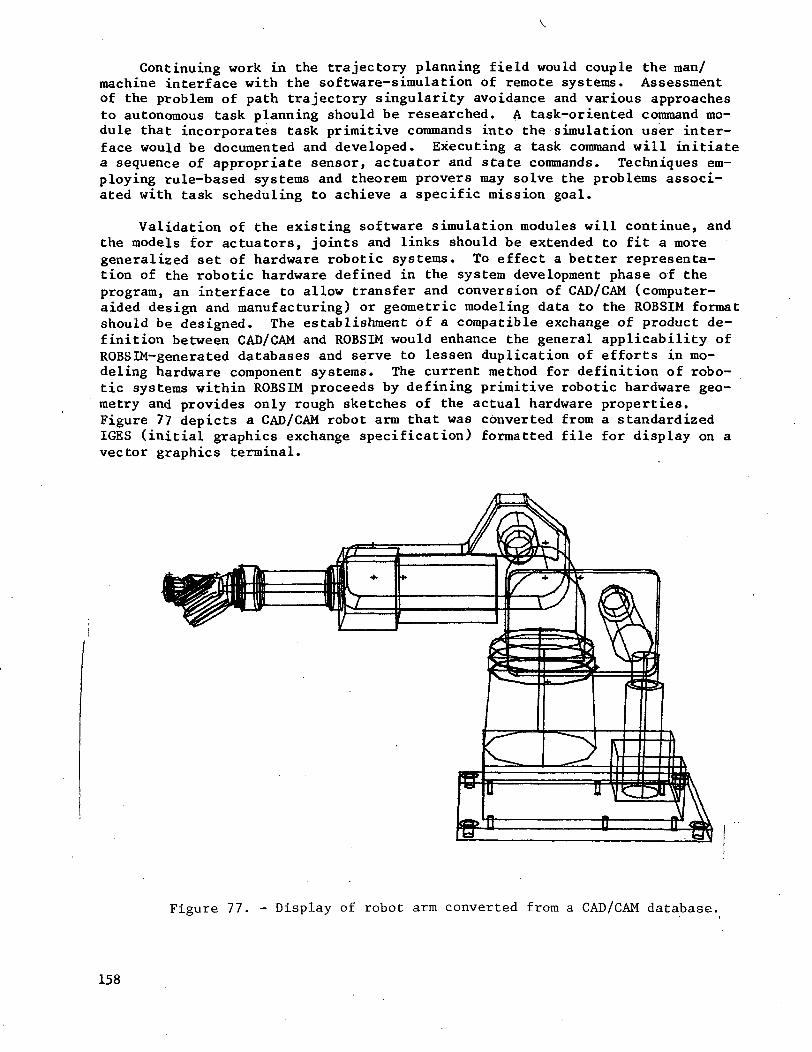
Continuing work in the trajectory planning field would couple the man/machine interface with the software-simulation of remote systems. Assessmentof the problem of path trajectory singularity avoidance and various approachesto autonomous task planning should be researched. A task-oriented command mo-dule that incorporates task primitive commands into the simulation user inter-face would be documented and developed. Executing a task command will initiatea sequence of appropriate sensor, actuator and state commands. Techniques em-ploying rule-based systems and theorem provers may solve the problems associ-ated with task scheduling to achieve a specific mission goal.
Validation of the existing software simulation modules will continue, andthe models for actuators, joints and links should be extended to fit a moregeneralized set of hardware robotic systems. To effect a better representa-tion of the robotic hardware defined in the system development phase of theprogram, an interface to allow transfer and conversion of CAD/CAM (computer-aided design and manufacturing) or geometric modeling data to the ROBSIM formatshould be designed. The establishment of a compatible exchange of product de-finition between CAD/CAM and ROBSIM would enhance the general applicability ofROBSIM-generated databases and serve to lessen duplication of efforts in mo-deling hardware component systems. The current method for definition of robo-tic systems within ROBSIM proceeds by defining primitive robotic hardware geo-metry and provides only rough sketches of the actual hardware properties.Figure 77 depicts a CAD/CAM robot arm that was converted from a standardizedIGES (initial graphics exchange specification) formatted file for display on avector graphics terminal.
Figure 77. - Display of robot arm converted from a CAD/CAM database.
158
Current processing capabilities in the ROBSIM program may be carried outon virtually any modern digital computing machine of the supermini or higherclass. However, with the exception of the newest and fastest machines, thenecessary speed for real-time simulation processing will not be achieved by asingle machine. Specialized machines with multiple processor architectureswill be necessary to accomplish this goal. Areas such as mechanical configu-ration optimization, accuracy analysis, control requirements, stability, andwork environment studies require simulation but not necessarily in real time.Several significant long-range requirements point to the need for a real-timesimulation capability, and research of the following available systems is re-commended:
1) Realistic graphics - When the simulation system is coupled with a gra-phics display of the computer solutions in real time, the results aremuch more realistic;
2) Surrogate hardware - Properly simulated hardware may be used to re-place hardware subsystems that have failed or are not yet available.The remainder of the hardware may be used in the system as intended.System problems may be isolated by substituting software modules forsuspected failing hardware modules. System integration may be ap-proached more gradually by bringing hardware on line one module at atime or as the hardware is available;
3) Real time testbed for algorithm development - Control and estimationalgorithms may be evaluated and optimized using the true or emulatedcontrol computer without the use of scaling within the algorithms, andwith no potential damage to the existing and manipulator assembly;
4) Real-time testbed for path planning and man/machine interface - Safe,real-time response to decisions and trajectory decisions as dictatedby sensor output and command input is very important for a smooth flowof the man/machine interface within the simulation and to achieve adiversified approach to task-oriented plans.
159
REFERENCES
Ballard, D. H.; and Brown, C. M.: Computer Vision. Prentice-Hall, Inc.,Englewood Cliffs, NJ, 1982.
Barker, L. Keith: Vector Algebra Approach to Extract Denavit-Hartenberg Para-meters of Assembled Robot Arms. NASA Technical Paper 2191, August 1983.
Binford, T. 0.: Inferring Surfaces from Images. Artificial Intelligence, vol.17, 1981, pp. 205-244.
Brady, M: Computational Approaches to Image Understanding. Computing Surveys,vol 14 (1), 1982, pp. 3-71.
Chace, M. A.; Calahan, D. A.; Orlandea, N.; and Smith, D.: Formulation andNumerical Methods in the Computer Evaluation of Mechanical Dynamic Systems.Third World Congress for the Theory of Machines and Mechanisms, Kupari,Yugoslavia, 1971, pp. 61-100.
Dubowsky, S.; and DesForges, D. T.: The Application of Model-Referenced Adap-tive Control to Robotic Manipulators. Joint Automatic Control Conference, 1979.
Duffy, J,; and Crane, C.: A Displacement Analysis of the General Spatial7-link, 7R Mechanism. Mechanism and Machine Theory, vol. 15, no. 3, 1980, pp.153-169.
Duffy, J,: Analysis of Mechanisms and Robot Manipulators. Wiley, New York,NY, 1981.
Duffy, J,: Analysis of Robot Arms. DOE Contract AC05-79ER-10013, Center ofIntelligent Machines and Robotics, University of Florida, Gainesville, FL,1979.
Franklin, G. F.; and Powell, J. D.: Digital Control of Dynamic Systems.Addison-Wesley Publishing Company, Menlo Park, CA, 1981.
Fukunaga, Keinosuke: Introduction to Statistical Pattern Recognition. AcademicPress, San Francisco, 1972, p. 294.
Goodwin, Graham C.; and Sin, K. S.: Adaptive Filtering Prediction and Control.Manuscript, Department of Electrical and Computer Engineering, University ofNewcastle, New South Wales, 2308, Australia, 1982.
Hanson, A. R.; and Riseman, E. M.: Processing Cones: A Computational Structurefor Image Analysis. Structured Computer Vision, ed. Tanimoto, S.; and Klinger,A.; Academic Press, New York, NY, 1980.
Hemani, J; and Camana, P. C.: Nonlinear Feedback in Simple Locomotion Systems.IEEE Transactions on Automatic Control, December 1976.
160
Hildreth, E. C.: Edge Detection for Computer Vision Systems. Mechanical Engi-neering, August 1982, pp. 48-53.
Hollerback, J. M.: A Recursive Lagrangian Formulation of Manipulator Dynamicsand a Comparative Study of Dynamics Formulation Complexity. IEEE Transactionson Systems, Man, and Cybernetics, vol. SMC-10, no. 11, 1980, pp. 730-736.
Horowitz, R.; and Tomizuka, M.: Discrete-Time Model Reference Adaptive Controlof Mechanical Manipulators. ASME Computer Engineering Conference, August,1982.
Hueckel, M. F.: An operator Which Locates Edges in Digitized Pictures. Jour-nal of the ACM, vol. 18, 1971, pp. 113-125.
Hummel, R. A.: Edge Detection Using Basic Functions. Technical Report TR-56,University of Maryland, Computer Science Center, August 1977.
Koivo, A. J.; and Guo, T. H.: Control of Robotic Manipulator with Adaptive Con-troller. Conference on Decision and Control, December 1981.
Kreisselmeier, G.: On Adaptive State Regulation. IEEE Transactions, vol.AC-27, no. 1, February 1982.
Lee, C. S. G.: Robot Arm Kinematics, Dynamics, and Control. Computer Maga-zine, December 1982, pp. 62-80.
Lee, C. S. G.; and Chung, M. J.: An Adaptive Control Strategy for MechanicalManipulators. Proceedings, 21st Conference on Decision and Control, 1982*
Lee, George: University of Michigan Department of Electrical and ComputerEngineering, Ann Arbor, MI. Personal Correspondence.
Leinenger, G. G.: Self-Tuning Adaptive Control of Manipulators. Symposium onAdvanced Software in Robotics, Liege, Belgium, 1983.
Lowrie, J. W.; Formelia, A. J.; Haley, D. C.; Gremban, K. D.; Van Baalen, J.;and Walsh, R. W.: Evaluation of automated Decisionmaking Methodologies andDevelopment for an Integrated Robotic System Simulation. NASA ContractorReport 165975, 1982.
Luh, J. Y. S.; Walker, M. W.; and Paul, R. P. C.: Resolved-Acceleration Con-trol of Mechanical Manipulators. IEEE Trans, vol. AC-25, no. 3, June 1980.
Luh, J. Y. S.; Walker, M. W.; and Paul, R. P. C.: Online Computational Schemefor Mechanical Manipulators. J. Dynamic System. Measurement. Contr., Trans-actions ASME, vol. 102, June 1980.
MacVicar-Whelan, P. J.; and Binford, T. 0.: Line Finding with Subpixel Preci-sion. Techniques and Applications of Image Understanding, ed. Pearson, J. J.;SPIE vol. 281, 1981, pp. 211-216.
Marr, D.; and Hildreth, E. C.: Theory of Edge Detection. Proceedings of theRoyal Society of London, Series B, 207, 1980, pp. 187-217.
161
Mason, M. T.: Compliance and Force Control for Computer-Controlled Manipula-tors. IEEE Transactions, vol. SMC-11, no. 6, June 1981.
Morgenthaler, D. G.: A New Hybrid Edge Detector. Computer Graphics and ImageProcessing, vol. 16, 1981, pp. 166-176.
Nevins, J. L.; and Whitney, D. E.: Computer-Controlled Assembly. ScientificAmerica, 1978.
Nishihara, K.; and Larson, W.: Towards a Real-Time Implementation of the Marrand Poggio Stereo Matcher. Techniques and Applications of Image Understanding,ed. Pearson, J. J.; SPIE vol. 281, 1981, pp. 299-305.
O'Gorman, F.: Edge Detection Using Walsh Functions. Artificial Intelligence,vol. 10, 1978, pp. 215-223.
Okada, T.: Computer Control of Multijointed Finger System for Precise ObjectHandling. IEEE Sys. Man. Cyber, vol. SMC-12, no. 3, 1982.
Orin, D. E.; McGhee, R. B,; Vukobratovic, M.; and Hartoch, G.: Kinematic andKinetic Analysis of Open-Chair linkages Utilizing Newton-Euler Methods. Mathe-matical Biosciences, vol. 43, 1979, pp. 107-130.
Paul, R. P.: Robot Manipulators: Mathematics, Programming, and Control. MITPress, Cambridge, Massachusetts, 1981a.
Paul, R. P.: Kinematic Control Equations for Manipulators. IEEE Transactions,vol. SMC-11, 1981b.
Paul, R. P.; MaRong; Hong Zhang: The Dynamics of the PUMA Manipulator. Ameri-can Control Conference Proceedings, 1983, pp. 491-496.
Peli, T.; and Malah, D.: A Study of Edge Detection Algorithms. Computer Gra-phics and Image Processing, vol. 20, 1982, pp. 1-21.
Prewitt, J. M. S.: Object Enhancement and Extraction. Picture Processing andPsychopictories, ed. Lipkin, B. S.; and Rosenfeld, A.; Academic Press, NewYork, NY, 1970.
Raibert, M. H.; and Craig, J. J.: Hybrid Position/Force Control of Manipula-tors. ASME Transactions, Journal of Dynamic Systems, Measurement, and Con-trol, vol. 102, pp. 126-133.
Rosenfeld, A.; and Kak, A. C.: Digital Picture Processing. Second Edition,Academic Press, New York, NY, 1982.
Rosenfeld, A.; and Thurston, M.: Edge and Curve Detection for Visual SceneAnalysis. IEEE Transactions, vol. C-20(5), 1972, pp. 562-569.
Salisbury, J. K.: Active Stiffness Control of Manipulator in Cartesian Coordi-nates. Proceedings of the 19th IEEE Conference of Decision and Control, 1980,pp. 95-100.
162
Shanraugan, K. S.; Dickey, F. M.; and Green, J. A.: An Optimal Frequency DomainFilter for Edge Detection in Digital Pictures. IEEE Transactions, vol. PAMI-1,1979, pp. 37-49.
Shimano, b. E.; and Roth, B.: On Force Sensing Information and Its Use in Con-trolling Manipulators. Proceedings of the 9th International Symposium on In-dustrial Robots, Washington, D.C., 1979. pp. 119-126.
Shirai, Y.: Recognition of Real-World Objects Using Edge Cues. Computer Vi-sion Systems, ed. Hanson, A. R.; and Riseman, E. M.; Academic Press, New York,NY, 1978.
Sugimoto, K.; Duffy, J,; and Hunt, K. H.: Special Configurations of SpatialMechanisms and Robots. Mechanism and Machine Theory, vol. 17, no. 2, 1982,pp. 119-132.
Thomas, M.; and Tesar, D.: Dynamic Modeling of Serial Manipulator Arms. ASMETransactions, Journal of Dynamic Systems, Measurement, and Control, vol. 104,1982, pp. 218-228.
Walker, M. W.; and Orin, D. E.: Efficient Dynamic Computer Simulation ofRobotic Mechanisms. ASME Transactions, Journal of Dynamic Systems, Measure-ments, and Control, vol. 104, 1982, pp. 205-211.
Whitney, D. E.: Resolved Motion Rate Control of Manipulators and Human Pros-thesis. IEEE Transactions, vol. MMS-10, no. 2, 1969, pp. 47-53.
Wu, C. H.; and Paul, R. P.: Resolved Motion Force Control of Robot Manipula-tor. IEEE Transactions, vol. SMC-12, no. 3, 1982, pp. 266-275.
163
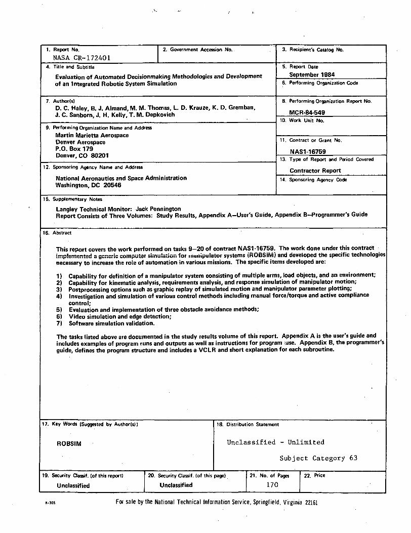
1. Report No.NASA CR- 172401
2. Government Accession No. .
4. Title and Subtitle
Evaluation of Automated Decisionmaking Methodologies and Developmentof an Integrated Robotic System Simulation
7. Author(s)D. C. Haley, B. J. Almand, M. M. Thomas, L. D. Krauze, K. D. Gremban,J. C. Sanborn, J. H. Kelly, T. M. Depkovich
9. Performing Organization Name and AddressMartin Marietta AerospaceDenver AerospaceP.O. Box 179Denver, CO 80201
12. Sponsoring Agency Name and Address
National Aeronautics and Space AdministrationWashington, DC 20546
3. Recipient's Catalog No.
5. Report DateSeptember 1984
6. Performing Organization Code
8. Performing Organization Report No.
MCR-84-549
10. Work Unit No.
11. Contract or Grant No.
N ASM 675913. T.ype of Report and Period Covered
Contractor Report
14. Sponsoring Agency Code
15. Supplementary Notes
Langley Technical Monitor: Jack PenningtonReport Consists of Three Volumes: Study Results, Appendix A-User's Guide, Appendix B-Programmer's Guide
16. Abstract
This report covers the work performed on tasks 9-20 of contract ISIAS1 -16759. The work done under this contractimplemented a generic computer simulation for rnanipuiaior systems (ROBSiM) and developed the specific technologiesnecessary to increase the role of automation in various missions. The specific items developed are:
1) Capability for definition of a manipulator system consisting of multiple arms, load objects, and an environment;2) Capability for kinematic analysis, requirements analysis, and response simulation of manipulator motion;3) Postprocessing options such as graphic replay of simulated motion and manipulator parameter plotting;4) Investigation and simulation of various control methods including manual force/torque and active compliance
control;5) Evaluation and implementation of three obstacle avoidance methods;6) Video simulation and edge detection;7) Software simulation validation.
The tasks listed above are documented in the study results volume of this report. Appendix A is the user's guide andincludes examples of program runs and outputs as well as instructions for program :use. Appendix B, the programmer'sguide, defines the program structure and includes a VCLR and short explanation for each subroutine.
17. Key Words (Suggested by Author(s))
ROBSIM
19. Security dassif. (of this report)
Unclassified
18. Distribution Statement
Unclassified - Unlimited
Subject Category 63
20. Security Classif . (of this page) 21 . No. of Pages
Unclassified 170
22. Price
For sale by the National Technical Information Service, Springfield. Virginia 22161