1

Message passing-based joint CFO and channelestimation in mmWave systems with one-bit ADCs

Nitin Jonathan Myers, Student Member, IEEE, and Robert W. Heath Jr., Fellow, IEEE.

Abstract—Channel estimation at millimeter wave (mmWave)carrier frequencies is challenging when large antenna arrays areused. Prior work has leveraged the sparse nature of millimeterwave channels via compressed sensing-based algorithms for chan-nel estimation. Most of these algorithms, though, assume perfectsynchronization and are vulnerable to phase errors that arise dueto carrier frequency offset and phase noise. Recently sparsity-aware, non-coherent beamforming algorithms that are robust tophase errors were proposed for narrowband phased array sys-tems with full resolution analog-to-digital converters. Such energybased algorithms, however, are not robust to heavy quantizationat the receiver. In this paper, we develop a joint carrier frequencyoffset and wideband channel estimation algorithm that is scalableacross different hardware architectures. Our method exploits thesparse nature of millimeter wave channels in the angle-delaydomain, in addition to compressibility of the phase error vector.We formulate the joint estimation as a quantized sparse bilinearoptimization problem and then use message passing for recovery.We also give an efficient implementation of a generalized bilinearmessage passing algorithm for the joint estimation in one-bitreceivers. Simulation results show that our method is able toestimate the frequency offset and the channel compressively, evenin the presence of phase noise.

Index Terms—Wideband channel estimation, carrier frequencyoffset, compressed sensing, message passing, one-bit receivers,mm-Wave

I. INTRODUCTION

Millimeter wave (mmWave) communication introduces newchallenges in the design of multiple-input multiple-output(MIMO) communication systems [1]. For instance, large an-tenna arrays at the transmitter (TX) and the receiver (RX)are necessary to meet the link budget requirements [2]. As aresult, the channel has a higher dimension compared to whatis typical in lower frequency MIMO systems, and must beestimated more frequently thanks to the smaller coherencetime [3]. Furthermore, cost and power consumption are majorissues at the larger bandwidths that accompany mmWave,primarily due to high resolution analog-to-digital converters(ADCs) [4]. Typical mmWave hardwares that limit powerconsumption at large bandwidths introduce compression inthe channel measurements. For example, the one-bit ADCarchitecture [4] allows access to the output of every antennaat the expense of heavy quantization. The compression ofchannel measurements and the use of large antenna arrayscomplicate signal processing at mmWave.

N. J. Myers (nitinjmyers@utexas.edu) and R. W. Heath Jr.(rheath@utexas.edu) are with the Wireless Networking and CommunicationsGroup, The University of Texas at Austin, Austin, TX 78712 USA. Thismaterial is based upon work supported in part by the National ScienceFoundation under grant numbers NSF-CNS-1702800, NSF-ECCS-1711702,and NSF-CNS-1731658, and by a gift from Huawei Technologies, Inc.

Compressed sensing (CS) [5] [6] is an efficient technique torecover sparse high-dimensional signals with few projections.As MIMO channel matrices at mmWave are sufficiently sparsewhen expressed in an appropriate dictionary, applying toolsfrom CS to mmWave channel estimation can potentially reducethe training overhead. CS-based sparse channel estimationalgorithms have been proposed for various hardware architec-tures [7]–[9]. Recent developments in approximate messagepassing [10] [11] have enabled channel estimation algorithmsin low resolution receivers [12]. Most CS-based channel es-timation algorithms, however, assume perfect synchronizationand may fail when there is any residual carrier frequency offset(CFO) or phase noise [13].

CFO and phase noise are hardware impairments that corruptthe phase of the channel measurements. The mismatch be-tween the carrier frequencies of the local oscillators at the TXand the RX results in CFO. Phase noise in the system arisesdue to short-term random fluctuations in the frequency of theoscillators. Both these non-idealities are larger at mmWavedue to the high carrier frequency and ignoring them canresult in significant channel estimation error [14]. Correctingfor the CFO and then performing channel estimation seemslike a possible solution. The disadvantage, however, is thatprior to beamforming or channel estimation, mmWave systemsoperate at very low signal-to-noise ratio (SNR), which canresult in significant error in the CFO estimate. Prior workhas considered joint CFO and channel estimation [15] [16] inlower frequency systems. These joint estimation algorithms,however, cannot be applied to typical mmWave systems dueto differences in the hardware architectures. Furthermore, theyare not designed to incorporate the sparse nature of mmWavechannels. Therefore, there is a need to design either phaseerror robust channel estimation algorithms, or joint CFO andchannel estimation algorithms that can exploit the sparsity ofmmWave channel.

Recent work on phase error robust channel estimation islimited to narrowband systems and has focussed on specificmmWave hardware. In [13], [17] and [18], phase error robustcompressive beamforming algorithms were proposed for theanalog beamforming architecture. In [13], phase tracking fol-lowed by phase error compensated compressive beamformingwas proposed. The compensation, however, was done priorbeamforming and therefore suffers from low SNR. The non-coherent algorithms in [17] and [18] are not robust to heavyquantization at the receiver. These algorithms cannot be usedin standard one-bit receivers because the amplitude informa-tion in the channel measurements is completely lost due toone-bit quantization with a zero threshold.

2

Recent joint CFO and sparse narrowband channel estima-tion algorithms in [14] and [19] require high computationalcomplexity when extended to wideband systems. In [14], weproposed a joint CFO and narrowband channel estimationalgorithm using third-order tensors [20]. We also developeda sparsity-aware joint estimation algorithm for the one-bitADC architecture in [19]. The main idea underlying ourapproach in [19] was to use the lifting technique [21] alongwith message passing for the joint estimation with one-bitchannel measurements. Extending the narrowband solutionsin [14] or [19] to typical wideband mmWave systems wouldrequire optimization over millions of variables, which may beprohibitive in a practical setting.

In this paper, we propose a quantized sparse bilinear for-mulation of the joint CFO and wideband channel estimationproblem, and solve it using message passing. We assume thata unique CFO and a unique phase noise process corrupt thechannel measurements. We also assume that there is perfectframe timing synchronization between the TX and the RX. Wesummarize the main contributions in this paper as follows.

• We formulate the joint CFO and wideband channel estima-tion problem as a noisy quantized sparse bilinear optimiza-tion problem. Our framework leverages the sparse nature ofthe wideband channel in the angle and delay domains, andalso exploits the compressibility of the phase error vectorin the frequency domain.

• To solve the non-convex problem at hand, we use thevector variance version of the Parametric Bilinear General-ized Approximate Message Passing (PBiGAMP) algorithm[22]. As a naive implementation of PBiGAMP can becomputationally expensive for typical mmWave settings, wederive a low complexity version of PBiGAMP by exploitingstructure in the joint estimation problem.

• We propose the concept of “CFO propagation” for thejoint CFO and channel estimation using circulant training.Although circulant training allows fast message passing withthe channel variables, it results in a non-identifiable jointestimation problem due to CFO propagation. We provethat any circulant training-based joint CFO and channelestimation technique that exploits channel sparsity in a DFT-based dictionary suffers from CFO propagation.

• We evaluate the performance of our joint estimation algo-rithm assuming a digital receiver architecture with one-bitADCs and compare it with the hypothetical full resolutioncase. Simulation results show that the proposed approach isable to recover both the channel and the CFO compressivelywith IID Gaussian- and IID QPSK-based training matrices,even in the presence of phase noise uncertainity.

Our algorithm is advantageous over the existing sparsity-awaremethods for joint estimation or phase error robust channelestimation in terms of the capability to efficiently handlefrequency selective channels and scalability to other mmWavearchitectures.

Notation: A is a matrix, a is a column vector and a, Adenote scalars. Using this notation AT ,A and A∗ representthe transpose, conjugate and conjugate transpose of A. The

matrices |A| and |A|2 contain the element-wise magnitude andsquared magnitude of the entries of A. We use A(i) and A(j)to denote the ith row and j th column of A. We use diag (a)to denote a diagonal matrix with entries of a on its diagonal.The scalar am denotes the mth element of a. The symbols⊗ and are used to denote the Kronecker product and theHadamard product. vec (A) is a vector obtained by stackingall the columns of A and vecm (A) denotes the mth element ofvec (A). We define Ai, j = veci

(A(j)

). We use IN to denote the

set 1, 2, 3, ..N. The matrix UN ∈ CN×N denotes the unitary

discrete Fourier transform matrix. N(m,R) is the probabilitydensity function of complex Gaussian random vector withmean m and covariance R. We define e`,N ∈ RN×1 as theN dimensional canonical basis vector with its `th coordinateas 1. The function sign(a) is 1 for a ≥ 0 and is −1 for a < 0.We define sinc(a) = sin(πa)/(πa).

II. SYSTEM AND CHANNEL MODELS

In this section, we describe the underlying hardware ar-chitecture, CFO and phase noise model, and the widebandmmWave channel model used for our simulations. In par-ticular, we focus on the digital receiver architecture withone-bit ADCs to highlight the differences with the existingnon-coherent algorithms. Nevertheless, our algorithm can beextended to other mmWave architectures as the underlyingjoint estimation problem is bilinear in nature.

A. System Model

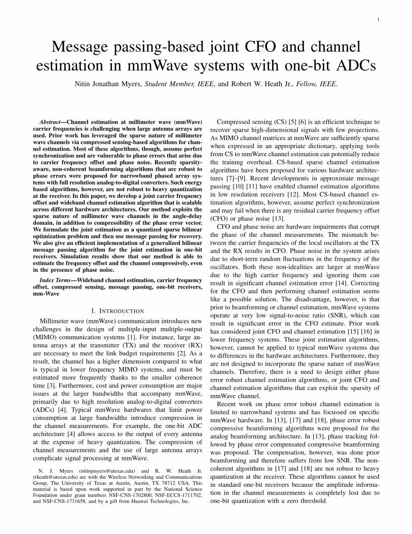
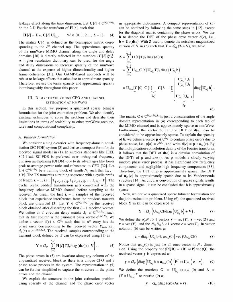
Fig. 1. A MIMO system with local oscillators operating at f1 and f2. Eachreceive antenna is associated with a radio frequency chain and a pair of q-bitADCs. In this paper, we consider the extreme cases of q = 1 and q = ∞.

We consider a MIMO system with uniform linear array ofNtx antennas at the TX and Nrx antennas at the RX, as shownin Fig. 1. We use linear arrays for a concise representationof the simplifications involved in PBiGAMP; our frameworkcan be extended to other array geometries using appropriatearray response vectors in the formulation. We do not imposeconstraints on the number of radio frequency (RF) chains orthe resolution of the digital-to-analog converters (DACs) atthe TX. The resolution of the Nrx ADCs at the RX, however,is assumed to be limited. We assume that all the RF chainsat the TX are driven by a single oscillator that operates ata carrier frequency of f1. In a practical mmWave system,multiple oscillators may be employed at the TX as the useof a single oscillator can result in a higher insertion loss

3

[23]. Even in such settings, our assumption is reasonable froma mathematical perspective as multiple colocated mmWaveoscillators at the TX can be synchronized to the same f1through calibration [24], [25]. The use of a single oscillatorat the RX can be justified using a similar argument. The RXdownconverts the received RF signal using a carrier frequencyf2, that slightly differs from f1. After downconversion at theRX, the output at each antenna is sampled using a pair of q-bit ADCs, one each for the in-phase and the quadrature phasecomponents. We use Qq (·) to represent the q-bit quantizationfunction corresponding to the ADCs. In this paper, we considerthe extreme case of q = 1 and provide a performancecomparison relative to q = ∞. The quantization functions forthe two cases are Q1 (x) = sign (real (x)) + j sign (imag (x))and Q∞ (x) = x. Note that the functions sign (·) , real (·) andimag (·) are applied element-wise on the vector.

The impact of CFO on channel estimation algorithms ismore significant in one-bit receivers than the full resolutionones. The mismatch in the carrier frequencies, i.e., | f2 − f1 | istypically in the order of several parts per millions (ppms) of f1or f2. Due to the high carrier frequencies at mmWave, evensuch small differences can significantly perturb the channelestimate when ignored [13]. For a symbol duration of T sec-onds, we define the digital domain CFO as ε = 2π ( f1 − f2)T .CFO results in unknown phase errors in the received samplesthat linearly increase with time. Hence, the impact of CFOon standard channel estimation algorithms is determined bythe length of training. As one-bit receivers relatively need alonger training for channel estimation when compared to thefull resolution ones, channel estimation algorithms that ignorephase errors are more vulnerable to the CFO in one-bit systemsthan the full resolution ones.

Phase noise in wireless systems arises due to jitter in thefrequency of the oscillators. In this paper, we assume thatphase noise occurs only at the receiver. Such an assumption isreasonable in broadcasting applications where a high qualityoscillator is used at the TX [26]. As is common in prior work,we model phase noise at the receiver as a Wiener processwith an innovation variance of β2 [27], [28]. Let φk denotethe phase error introduced in the k th received sample due tophase noise at the RX. In a Wiener process, the innovations inthe phase error, i.e., φk − φk−1, are modeled as IID Gaussianrandom variables with zero mean and variance β2. For such aprocess, it can be observed that the variance of φk linearlyincreases with k. As β2 is proportional to f 2

2 [13], phasenoise is higher at mmWave carrier frequencies for a givenquality of oscillator. We assume a unique phase noise processat the receiver. Such an assumption is valid only when asingle oscillator drives all the RF chains at the receiver. Whenmultiple oscillators are used at the RX, the impact of phasenoise on the received signal is more complicated. Althoughcalibration of multiple oscillators at the RX can achieve localcarrier frequency synchronization [24], [25], it may not resultin the same random phase noise process across all the RFchains. Our assumption regarding a unique phase noise processis perhaps simplistic, but we leave the development of newjoint estimation techniques that account for multiple phasenoise processes to future work.

Now, we describe the received signal model in the digitalreceiver architecture. Let t [n] ∈ CNtx×1 be the nth transmitsymbol satisfying the power constraint E [t∗ [n] t [n]] = P. Thediscrete time baseband representation of the MIMO channelis assumed to be limited to L taps. Let H [`] ∈ CNrx×Ntx

be the `th tap of the equivalent baseband channel, where` ∈ 0, 1, 2, ..., L − 1. Under the perfect frame timing syn-chronization assumption, the sampled baseband vector in thenth symbol duration can be given by

Y(n) = Qq

(e j(εn+φn)

L−1∑=0

H [`] t [n − `] + V(n)

), (1)

where V(n) ∼ N(0, σ2INrx ) is additive white Gaussian noise.In this paper, we develop an algorithm to estimate ε andH [`]L−1

`=0 from the series of observations Y(n). Our jointestimation algorithm can be extended to any q-bit ADC ar-chitecture by defining appropriate output likelihood functionsin message passing.

B. Channel Model

We consider a clustered channel model for the frequency se-lective mmWave MIMO channel. The channel consists of Ncsclusters with Mn rays in the nth cluster. Let γn,m, τn,m, θr,n,mand θt,n,m denote the complex gain, delay, angle-of-arrival(AoA) and angle-of-departure (AoD) of the mth ray in the nth

cluster. We assume that the transmitted signal is bandlimitedto 1/T Hz. With ωr,n,m = π sin θr,n,m, ωt,n,m = π sin θt,n,m, andthe Vandermonde vector

aN (∆) =[1 , e j∆ , e j2∆ , · · · , e j(N−1)∆

]T, (2)

the `th tap of the wideband MIMO channel for a half wave-length spaced uniform linear array is given by

H [`] =Ncs∑n=1

Mn∑m=1

γn,maNrx

(ωr,n,m

)a∗

Ntx

(ωt,n,m

)sinc

(` −

τn,m

T

).

(3)The wideband channel can be represented using NrxNtxL com-plex entries, and the matrix in (3) is large in typical mmWavesystems. The channel impulse response in (3) is representedusing a linear combination of bandlimited sinc(·) functions.Notice that each of these sinc(·) functions is delayed by thenormalized delay spread, i.e, τn,m/T and evaluated at periodictime instants to obtain the discrete time representation in (3).Other filtering functions could also be used to incorporate theeffect of pulse shaping at the TX or filtering at the RX [29].

The mmWave MIMO channel is aproximately sparse in anappropriate dictionary due to the propagation characteristicsof the environment at mmWave frequencies. Compared tothe lower frequency channels, mmWave channels compriseof fewer clusters [4]. Each of the channel taps H [`], isapproximately sparse in the spatial Fourier basis at mmWave[12]. Furthermore, the channel is approximately sparse alongthe time dimension as the delays of the propagation rays areheavily clustered within the delay spread. As the delays τn,mmay not necessarily be an integer multiple of T , there is a

4

leakage effect along the time dimension. Let C [`] ∈ CNrx×Ntx

be the 2-D Fourier transform of H [`], such that

H [`] = UNrxC [`]U∗Ntx, ∀` ∈ 0, 1, 2, ..., L − 1 . (4)

The matrix C [`] is defined as the beamspace matrix corre-sponding to the `th channel tap. The approximate sparsityof the mmWave MIMO channel along the angle and delaydomains [30] is directly reflected in the matrices C [`]L−1

`=0 .A higher resolution dictionary can be used for the angleand delay dimensions to increase sparsity of the mmWavechannel at the expense of higher dimensionality and higherframe coherence [31]. Our GAMP-based approach will berobust to leakage effects that arise due to approximate sparsity.Therefore, we use the terms sparsity and approximate sparsityinterchangeably throughout this paper.

III. DEMYSTIFYING JOINT CFO AND CHANNELESTIMATION AT MMWAVE

In this section, we propose a quantized sparse bilinearformulation for the joint estimation problem. We also identifyexisting techniques to solve the problem and describe theirlimitations in terms of scalability to other mmWave architec-tures and computational complexity.

A. Bilinear formulation

We consider a single-carrier with frequency-domain equal-ization (SC-FDE) system [3] and derive a compact form for thereceived signal model in (1). In wireless standards like IEEE802.11ad, SC-FDE is preferred over orthogonal frequencydivision multiplexing (OFDM) due to its advantages like lowerpeak-to-average power ratio and robustness to CFO [32]. LetT ∈ CNtx×Np be a training block of length Np such that T(k) =t [k]. The TX transmits a training sequence with a cyclic prefixof length L − 1, i.e.,

[T(Np−L+2),T(Np−L+3), ...,T(Np),T

]. The

cyclic prefix padded transmission gets convolved with thefrequency selective MIMO channel before sampling at thereceiver. As usual, the first L − 1 samples of the receivedblock that experience interference from the previous transmitblock are discarded [3]. Let Y ∈ CNrx×Np be the receivedblock obtained after discarding the first L−1 received vectors.We define an ` circulant delay matrix J` ∈ CNp×Np , suchthat its first column is the canonical basis vector e1+`,Np . Wedefine a vector d(ε) ∈ CNp such that its nth entry has thephase error corresponding to the received vector Y(n), i.e.,dn(ε) = e j(εn+φn). The received samples corresponding to thetransmit block defined by T can be expressed using (1) as

Y = Qq

(L−1∑=0

H [`]TJ`diag (d(ε)) + V

). (5)

The phase errors in (5) are invariant along any column of theunquantized received block as there is a unique CFO and aphase noise process in the system. The representation in (5)can be further simplified to capture the structure in the phaseerrors and the channel.

We exploit the structure in the joint estimation problemusing sparsity of the channel and the phase error vector

in appropriate dictionaries. A compact representation of (5)can be obtained by following the same steps in [12], exceptfor the diagonal matrix containing the phase errors. We useb to denote the DFT of the phase error vector d(ε), i.e.,b = UNpd(ε). With Z used to denote the noiseless unquantizedversion of Y in (5) such that Y = Qq (Z + V), we have

Z =L−1∑=0

H [`]TJ` diag (d(ε))

=

L−1∑=0

UNrxC [`]U∗NtxTJ` diag

(U∗Np

b)

= UNrx [C [0] C [1] · · ·C [L − 1]]︸ ︷︷ ︸∆=C

U∗Ntx

TJ0U∗Ntx

TJ1...

U∗NtxTJL−1

︸ ︷︷ ︸∆=F

diag(U∗Np

b).

(6)

The matrix C ∈ CNrx×NtxL is just a concatenation of the angledomain representation in (4) corresponding to each tap ofthe MIMO channel and is approximately sparse at mmWave.Furthermore, the vector b, i.e., the DFT of d(ε), can beconsidered to be approximately sparse. To explain the sparsityof b, we define a vector p ∈ CNp to contain phase errors due tophase noise, i.e., p[n] = e jφn , and write d(ε) = p aN (ε). Bythe multiplication-convolution duality of the Fourier transform,it follows that the DFT of d(ε) is a circular convolution ofthe DFTs of p and aN (ε). As p models a slowly varyingrandom phase error process, it has significant low frequencycomponents and negligible high frequency components [33].Therefore, the DFT of p is approximately sparse. The DFTof aN (ε) is approximately sparse due to its Vandermondestructure [14]. As circular convolution of sparse signals resultsin a sparse signal, it can be concluded that b is approximatelysparse.

Now, we derive a quantized sparse bilinear formulation forthe joint estimation problem. Using (6), the quantized receivedblock Y in (5) can be expressed as

Y = Qq

(UNrxCFdiag

(U∗Np

b)+ V

). (7)

We define the NpNrx × 1 vectors y = vec (Y), z = vec (Z) andv = vec (V), and the NrxNtxL × 1 vector c = vec (C). In vectornotation, (6) can be written as

z = diag(U∗Np

b ⊗ aNrx (0))

vec(UNrxCF

). (8)

Notice that aNrx (0) is just the all ones vector in Nrx dimen-sion. Using the property vec (PQR) =

(RT ⊗ P

)vec (Q), the

received vector y is expressed as

y = Qq

(diag

(U∗Np

b ⊗ aNrx (0)) (

FT ⊗ UNrx

)c + v

). (9)

We define the matrices G = U∗Np⊗ aNrx (0) and A =(

F ⊗ UNrx

)T to rewrite (9) as

y = Qq (diag (Gb)Ac + v) . (10)

5

Estimating the phase errors and the channel is equivalent toestimating b and c from y in (10). The joint estimation problemin (10) can be observed to be a noisy quantized bilinearproblem in b and c, subject to the sparsity of b and c.

B. Limitations of existing techniques

1) CFO robust methods: Existing sparse channel estima-tion methods that are robust to CFO discard the phase ofthe channel measurements. A hashing technique based non-coherent beam alignment algorithm was proposed in [17] foranalog beamforming systems. This method, however, assumesfine control over the phase shifters, which is not necessarilythe case with mmWave systems. The received signal strength-based method in [18] accounts for the limited phase controland uses pseudo-random phase shifts for compressive beam-training. The solutions in [17] and [18] assume a narrowbandmmWave system and perform beam-alignment with just themagnitude of the channel measurements. These methods,however, cannot be used in standard one-bit receivers that usea zero threshold, as energy detection with undithered one-bitADCs is not feasible unless additional circuit components areused. For example, Q1 (r) and Q1 (α r) are the same for anyα > 0. As the only information provided by an unditheredone-bit ADC is phase quantized to 4 levels, discarding it dueto phase errors leaves no information.

2) Joint estimation using lifting: Lifting [21] [34] is a con-vex relaxation technique that transforms a bilinear problem toa higher dimensional one and then recovers the original vectorsby solving the higher dimensional problem. We describe thelifting technique applied to the joint estimation problem in(10). With M denoting the number of entries in y or z, i.e.,M = NrxNp, the mth entry of z can be written as

zm = vecm (diag (Gb)Ac) (11)

= G(m)bA(m)c (12)

= G(m)bcT(A(m)

)T(13)

=(A(m) ⊗ G(m)

)vec

(bcT

), ∀m ∈ IM . (14)

We define a lifted variable x = vec(bcT

)and a measurement

matrix Φ ∈ CM×NpNrxNtxL , such that Φ(m) = A(m) ⊗ G(m).Hence, the quantized measurements in (10) can be expressedas

y = Qq (Φx + n) . (15)

The lifted vector x in (15) is sparse as it is just an outerproduct [20] of the sparse vectors b and c. Several CS-basedalgorithms [6] [35] can be used to recover x from the possiblyunder-determined noisy quantized system in (15). Using theSVD of the higher dimensional matrix estimate, the vectorsin the joint estimation problem can be estimated upto a scalefactor.

Lifting followed by the SVD was applied to joint CFO andnarrowband channel estimation for one-bit receivers in ourprevious work [19]. The main issue in extending our methodin [19] to wideband systems arises due to the large dimen-sionality of the lifted problem. For instance, the dimension ofx to perform joint CFO and channel estimation in wideband

systems would be NrxNtxNpL. Using lifting necessarily impliessolving for millions of variables for typical wideband mmWavesystems, due to the large number of antennas and the need foradditional pilots to compensate for the heavy quantization inlow resolution systems.

The limitations of the existing phase error robust and jointestimation solutions in terms of architectural scalability andcomputational complexity, motivate the need to develop newlow complexity joint estimation algorithms that can be appliedto wideband systems and low resolution receivers.

IV. MESSAGE PASSING BASED JOINT CFO AND CHANNELESTIMATION

In this section, we give a brief introduction to PBiGAMP[22] and discuss its application to the quantized sparse bilinearproblem in (10). We exploit the inherent structure in ourproblem to derive a low complexity and memory efficientimplementation of PBiGAMP for the joint estimation. Fur-thermore, we explain the CFO propagation effect induced bycirculant training matrices that prevents further reduction inthe computational complexity.

A. Introduction to PBiGAMP

The joint estimation problem in (10) can be solved usingPBiGAMP [22] by considering b, c, z and y of (8) and (10)as realizations of random vectors, say b, c, z and y. Let bi ,ck , zm and ym be the elements of these random vectors. Ingeneral, deriving the closed form Minimum Mean-SquaredError (MMSE) estimates [36] of b and c is difficult as itrequires marginalizing the joint PDF of b and c conditionedon y = y. Using ideas from message passing, PBiGAMPcan obtain the MMSE estimates of both the vectors in thequantized sparse bilinear problem.

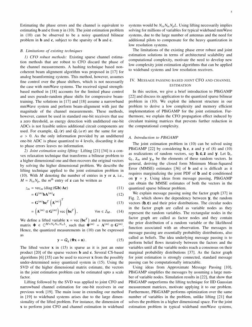
We explain message passing using the factor graph [37] inFig. 2, which shows the dependency between y, the randomvectors (b, c) and their prior distributions. The circular nodesin the factor graph are called as variable nodes as theyrepresent the random variables. The rectangular nodes in thefactor graph are called as factor nodes and they containthe prior distribution of a random variable or the likelihoodfunction associated with an observation. The messages inmessage passing are essentially probability distributions, alsocalled as beliefs. The idea underlying message passing is toperform belief flows iteratively between the factors and thevariables until all the variable nodes reach a consensus on theirmarginal probability distributions [37]. As the factor graphfor joint estimation is strongly connected, standard messagepassing can be computationally intractable.

Using ideas from Approximate Message Passing [10],PBiGAMP simplifies the messages by assuming a large num-ber of variable nodes. Simulation results in [22], that show thatPBiGAMP outperforms the lifting technique for IID Gaussianmeasurement matrices, motivate applying it to our problem.Furthermore, PBiGAMP performs optimization over the samenumber of variables in the problem, unlike lifting [21] thatsolves the problem in a higher dimensional space. For the jointestimation problem in typical wideband mmWave systems,

6

PBiGAMP is memory efficient over lifting by several ordersof magnitude.

!"#$"%

!"#$"%

&#'()#*$$+

,-./0#$.%!"##$%"# !"##$%"#

1*2..()

32"#24)(%

56./*"$.#720#$.

32"#24)(%

Fig. 2. The factor graph of quantized sparse bilinear message passing forjoint CFO and channel estimation. The rectangular nodes, called as factors,contain the likelihood functions corresponding to the received samples or thesparse priors. Messages are sent between the factor nodes and the variablenodes until the marginal probability distributions of the variables converge.

B. PBiGAMP for joint estimation

In this section, we explicitly state PBiGAMP [22] for jointestimation in (10) and describe the information contained inthe factor nodes of Fig. 2. To be consistent with the notationused in [22], we rewrite the random variable dependencycorresponding to (11) in the tensor notation as

zm =Nb∑i=1

Nc∑k=1

z(i,k)m bick, (16)

where Nb = Np, Nc = NrxNtxL, and z(i,k)m is an element of athird order tensor given by

z(i,k)m = Gm,iAm,k . (17)

As ym = Qq(zm + vm), the output likelihood function corre-sponding to the mth channel measurement, i.e., pym |zm (ym | z),can be expressed as

pym |zm (ym | z) =F

(√2sign(Reym )Rez

σ

)F

(√2sign(Imym )Imz

σ

)q = 1

1πσ2 e−

‖ym−z ‖2

σ2 q = ∞,

(18)

where F (·) is the cumulative distribution function of thestandard normal distribution. The factor nodes in Fig. 2, thatcontain likelihood functions in (18), ensure that the solutionto the bilinear problem is faithful to the observed channelmeasurements.

The sparsity of the vectors b and c is incorporated byassuming parametrized Bernoulli-Gaussian (BG) distributionsfor their priors pb (b) and pc (c). Prior work on linear CS hasshown that message passing with BG distributions can performbetter sparse recovery than LASSO in many settings [38]. InGAMP-based channel estimation [12], the BG distribution was

successfully used as a generative prior for mmWave channelsthat are approximately sparse. For simplicity, it is assumedthat each entry of b is independent of the other and identicallydistributed as pb. Similarly, the entries of c are assumed tobe IID, with pc as the distribution. Furthermore, the vectorsb and c are assumed to be independent of each other. Let λband λc denote the sparsity fraction of b and c. Let σ2

b andσ2

c be the variances of the coefficients corresponding to thenon-zero support of the vectors b and c. With δ (x) used torepresent the Dirac-delta function, the BG distributions pb andpc can be given as

pb (x) = λbδ (x) + (1 − λb)N(0, σ2b ), (19)

pc (x) = λcδ (x) + (1 − λc)N(0, σ2c ). (20)

It can be observed from (19) that each entry of b is 0 witha probability of λb and is distributed as Gaussian otherwise.As a result, the BG priors in (19) and (20) can model sparsevectors for an appropriate λb and λc.

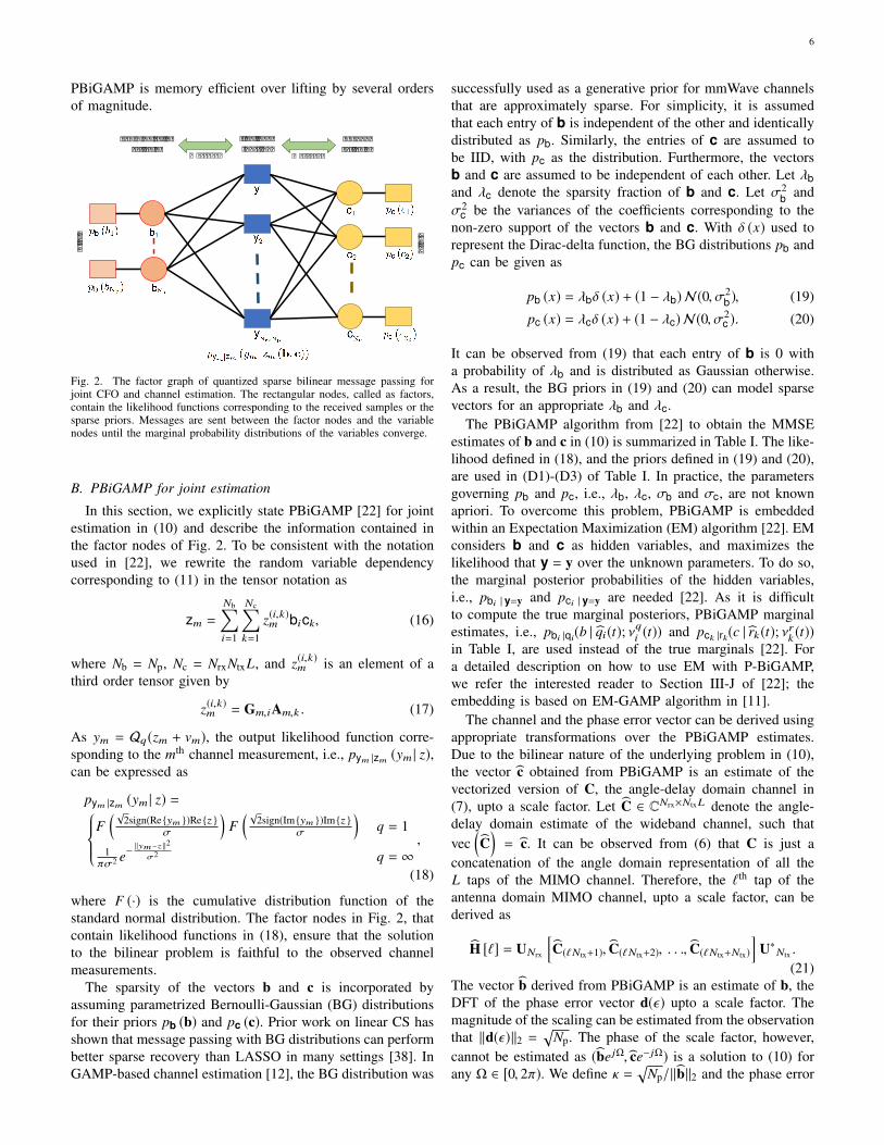
The PBiGAMP algorithm from [22] to obtain the MMSEestimates of b and c in (10) is summarized in Table I. The like-lihood defined in (18), and the priors defined in (19) and (20),are used in (D1)-(D3) of Table I. In practice, the parametersgoverning pb and pc, i.e., λb, λc, σb and σc, are not knownapriori. To overcome this problem, PBiGAMP is embeddedwithin an Expectation Maximization (EM) algorithm [22]. EMconsiders b and c as hidden variables, and maximizes thelikelihood that y = y over the unknown parameters. To do so,the marginal posterior probabilities of the hidden variables,i.e., pbi | y=y and pci | y=y are needed [22]. As it is difficultto compute the true marginal posteriors, PBiGAMP marginalestimates, i.e., pbi |qi

(b | qi(t); νqi (t)) and pck |rk(c | rk(t); νrk (t))in Table I, are used instead of the true marginals [22]. Fora detailed description on how to use EM with P-BiGAMP,we refer the interested reader to Section III-J of [22]; theembedding is based on EM-GAMP algorithm in [11].

The channel and the phase error vector can be derived usingappropriate transformations over the PBiGAMP estimates.Due to the bilinear nature of the underlying problem in (10),the vector c obtained from PBiGAMP is an estimate of thevectorized version of C, the angle-delay domain channel in(7), upto a scale factor. Let C ∈ CNrx×NtxL denote the angle-delay domain estimate of the wideband channel, such thatvec

(C)= c. It can be observed from (6) that C is just a

concatenation of the angle domain representation of all theL taps of the MIMO channel. Therefore, the `th tap of theantenna domain MIMO channel, upto a scale factor, can bederived as

H [`] = UNrx

[C(`Ntx+1), C(`Ntx+2), . . ., C(`Ntx+Ntx)

]U∗Ntx .

(21)The vector b derived from PBiGAMP is an estimate of b, theDFT of the phase error vector d(ε) upto a scale factor. Themagnitude of the scaling can be estimated from the observationthat ‖d(ε)‖2 =

√Np. The phase of the scale factor, however,

cannot be estimated as (be jΩ, ce−jΩ) is a solution to (10) forany Ω ∈ [0, 2π). We define κ =

√Np/‖b‖2 and the phase error

7

Definitions:pzm |pm

(z | p;νp

),

pym |zm(ym | z)N(z ;p,νp )∫z′ pym |zm(ym | z

′)N(z′;p,νp ) (D1)

pck |rk(c | r ;νr ) , pc(c)N(c;r,νr )∫c′ pc(c′)N(c′;r,νr )

(D2)

pbi |qi(b | q;νq ) , pb(b)N(b;q,νq )∫b′ pb(b

′)N(b′;q,νq ) (D3)

Initializations:∀m : sm(0) = 0 (I1)

∀i, k : choose bi (1), νbi (1), ck (1), νck(1) (I2)

for t = 1, . . .Tmax

∀m, i : z(i,∗)m (t) =∑Nc

k=1 z(i,k)m ck (t) (R1)

∀m, k : z(∗,k)m (t) =∑Nb

i=1 bi (t)z(i,k)m (R2)

∀m : z(∗,∗)m (t) =∑Nb

i=1 bi (t)z(i,∗)m (t) or

∑Nck=1 ck (t)z

(∗,k)m (t) (R3)

∀m : νpm(t) =∑Nb

i=1 νbi (t) |z

(i,∗)m (t) |2 +

∑Nck=1 ν

ck(t) |z

(∗,k)m (t) |2 (R4)

∀m : νpm(t) =νpm(t) +

∑Nbi=1 ν

bi (t)

∑Nck=1 ν

ck(t) |z

(i,k)m |2 (R5)

∀m : pm(t) = z(∗,∗)m (t) − sm(t−1)νpm(t) (R6)

∀m : νzm(t) = varzm | pm = pm(t);νpm(t) (R7)∀m : zm(t) = Ezm | pm = pm(t);νpm(t) (R8)∀m : νsm(t) = (1 − νzm(t)/ν

pm(t))/ν

pm(t) (R9)

∀m : sm(t) = (zm(t) − pm(t))/νpm(t) (R10)

∀k : νrk(t) =

( ∑Mm=1 ν

sm(t) |z

(∗,k)m (t) |2

)−1(R11)

∀k : rk (t) = ck (t) + νrk (t)∑M

m=1 sm(t)z(∗,k)m (t)∗

− νrk(t)ck (t)

∑Mm=1 ν

sm(t)

∑Nbi=1 ν

bi (t) |z

(i,k)m |2 (R12)

∀i : νqi (t) =( ∑M

m=1 νsm(t) |z

(i,∗)m (t) |2

)−1(R13)

∀i : qi (t) = bi (t) + νqi (t)

∑Mm=1 sm(t)z

(i,∗)m (t)∗

− νqi (t)bi (t)

∑Mm=1 ν

sm(t)

∑Nck=1 ν

ck(t) |z

(i,k)m |2(R14)

∀k : νck(t+1) = varck | rk = rk (t);νrk (t) (R15)

∀k : ck (t+1) = Eck | rk = rk (t);νrk (t) (R16)∀i : νbi (t+1) = varbi | qi = qi (t);ν

qi (t) (R17)

∀i : bi (t+1) = Ebi | qi = qi (t);νqi (t) (R18)

if∑M

m=1 |z(∗,∗)m (t) − z

(∗,∗)m (t−1) |2 ≤ τstop

∑Mm=1 |z

(∗,∗)m (t) |2, stop (R19)

endOutput: b = b (t) , c = c (t) , T = t .

TABLE ITHE PBIGAMP ALGORITHM FROM [22].

vector estimate as d = κU∗Npb. As d and d can differ in a

global phase, i.e., Ω, the nth entry of d can be modeled as

d[n] = e j(εn+φn+Ω) + w[n], (22)

where w[n] is a zero mean IID noise process. We use thescalar variance approximation in PBiGAMP [22] to computethe variance of w[n] as vw = κ2 ∑Nb

i=1 vib(T)/Np. Now, ε and Ω

in (22) are considered as state space variables to be estimatedfrom d [39]. The phase error in (22), i.e., εn + φn + Ω, is alinear function of the state space variables that is perturbed byan unknown Wiener phase noise. The nth observation in (22)is a noisy non-linear function of the phase error. For the statespace definitions and the model in (22), we use an extendedKalman filter (EKF) [39] to estimate ε from d. A detailedtreatment on how to apply EKF to (22) can be found in [13].

In this paper, we exploit the compressibility of the phaseerror vector in the DFT basis for joint estimation. It is possible,however, to incorporate the statistics of the phase noise byreplacing the nodes corresponding to b in Fig. 2 with the phaseerror variables and adding factors corresponding to the phasenoise process. In such case, the message passing algorithmmust handle the non-linear dependence of z on the phaseerrors.

C. PBiGAMP: From theory to practice

A standard implementation of the algorithm in Table I ismemory and computationally intensive as it involves repeatedoperations over a third order tensor [22]. In this section, weprovide insights into the key equations of Table I, and describeour low complexity implementation for joint CFO and channelestimation.

The equations in PBiGAMP are essentially determined bythe belief flows from the factor nodes to the variable nodes,and vice versa. Without loss of generality, we describe themessage flow between the variable node b1 and the factornode y1 in Fig. 2. In standard message passing, the messagesent from a factor node to b1 essentially represents the PDF ofb1 presumed by that factor node. In a fully connected factorgraph, the node b1 receives messages from all the M factornodes (yiMi=1) in addition to its prior distribution pb. As b1receives several beliefs from different factors, the belief sentby b1 to y1 is just a normalized product of all the beliefsreceived by b1 except the one from y1. For generic priors andlikelihood functions in the factor graph, performing standardmessage passing can be difficult as the belief flows are flowsof PDFs that are functions.

PBiGAMP simplifies standard message passing using thecentral limit theorem (CLT) and the Taylor series approxima-tion. Notice that y1 receives beliefs from all its neighbouringvariable nodes and contains the likelihood function in itself.The belief sent from y1 to b1 is computed by multiplyingthe likelihood function, with all the incoming beliefs to y1except the one from b1, and then integrating over all therandom variables except b1. The multiplication followed byintegration essentially yields the PDF of b1 presumed by thefactor node y1. The integration is often multidimensional andcan be difficult to compute. If y1 depends on a large numberof independent variable nodes through a linear function, thenthe linear combination can be approximated as a Gaussianrandom variable using the CLT [10]. In such case, the variablenodes can send just the mean and variances of the PDFs tothe factors and this information is sufficient to compute themean and variance of the Gaussian random variable, as seenin (R3) and (R5) of Table I. The message sent from y1 to b1can now be computed by multiplying the likelihood at y1 withthe compound Gaussian PDF, and marginalizing the productwith respect to b1. In general, the likelihood function can benon-linear in nature and can yield a complicated PDF of b1[22]. Using a second order Taylor series expansion for thelog PDF [10], PBiGAMP simplifies the belief sent from y1 tob1 to a Gaussian whose mean and variance can be computedfrom (R7)-(R9) of Table I. For q-bit ADCs, the closed formexpressions for the conditional mean and variance in (R7)and (R8) can be found in [40, Appendix A]. Unlike standardmessage passing, PBiGAMP is computationally tractable asthe messages contain just the mean and variances of the PDFs.

After several approximate message flows between the factornodes and the variable nodes, PBiGAMP is expected toconverge. The MMSE of b1 is computed as the expectation ofthe effective marginal, i.e., the normalized product of all the MGaussian PDFs received by b1 from the factor nodes and the

8

Operation Complexity

UNrx C (t)F O(NrxNtxLNp

)U∗Np

b (t) O(NplogNp

)(R3), (R13) O

(NrxNp

)(R4), (R5), (R11) O

(NtxLNp

)(R12), (R14) O

(NrxNtxLNp

)TABLE II

COMPLEXITY OF A SINGLE PBIGAMP ITERATION USING A FASTIMPLEMENTATION.

prior distribution on b1. Notice that the normalization has tobe done to ensure that the PDF integrates to 1. The expectationstep for the MMSE of b1 is given in (R18) using (R11) and(R12) as the intermediate steps. Similarly, the expectation forthe MMSE of c1 is given in (R16) using (R13) and (R14) asthe intermediate steps. Thus, PBiGAMP provides estimates ofthe vectorized sparse channel and the DFT of the phase errorvector.

The generic implementation of PBiGAMP is computation-ally expensive primarily due to (R1), (R2), (R5), (R12) and(R14) in Table I. It can be verified that each of these operationshave a complexity of O

(N2

rxN2p NtxL

)for a single PBiGAMP

iteration to perform joint estimation. For instance, (R1) re-quires computing the scalar z(i,∗)m (t) for every m ∈ IM andi ∈ INb , Therefore, (R1) demands O(MNbNc) computations,as each scalar computation requires Nc multiplications. AsM = NrxNp, Nb = Np and Nc = NrxNtxL for the jointestimation, (R1) has a complexity of O

(N2

rxN2p NtxL

)for

every PBiGAMP iteration. By exploiting the structure in thejoint estimation problem, the complexity of PBiGAMP canbe significantly reduced. A detailed description on our lowcomplexity implementation can be found in the Appendix. Ourimplementation exploits the Kronecker product structure of Gand A in (17), and the fast Fourier transform.

The complexity of PBiGAMP operations in our implemen-tation is summarized in Table II. The entries in Table IIare found using the complexity of matrix multiplicationsand FFTs. It can be noticed that the overall complexityof PBiGAMP using our implementation is O

(NrxNpNtxL

),

thereby achieving a speedup factor of NpNrx compared to thegeneric implementation. After all possible simplifications ofPBiGAMP for joint estimation, training design is possiblythe only frontier that can be exploited to further reduce thecomputational complexity.

D. CFO propagation effect: A barrier to complexity reductionwith circulant training

In this section, we explain how a reasonable training so-lution that allows a low complexity implementation does notpermit joint estimation. For simplicity of exposition, we con-sider a narrowband system, i.e., L = 1. We define H ∈ CNrx×Ntx

as the narrowband channel and C = U∗NrxHUNtx as its angle

domain representation.The complexity of our PBiGAMP implementation is deter-

mined by matrix multiplications with F, a matrix constructedfrom the Ntx×Np training matrix T. For the narrowband setting,

it can be observed from (6) that F = U∗NtxT. For a generic

matrix M ∈ CNrx×Ntx , standard matrix multiplication in MFrequires a complexity of O(NrxNtxNp). A possible approachto reduce this complexity is to set Np = Ntx, and choose Tas an Ntx × Ntx circulant training matrix [12]. When T isa circulant matrix, it can be diagonalized using the DFT asU∗Ntx

TUNtx = ΛT, where ΛT is a diagonal matrix. Equivalently,U∗Ntx

T = ΛTU∗Ntxor F = ΛTU∗Ntx

. The matrix MF is thenMΛTU∗Ntx

. As a result, the fast Fourier transform can be usedto compute MF for a complexity of O(NrxNtxlogNtx). In thissection, we show that circulant training is not suitable forthe joint estimation problem in (10) as it results in CFOpropagation.

The CFO propagation effect results in a class of sparsechannels and CFOs that are consistent with the observedchannel measurements. To explain this effect, we define Λε =

diag(d(ε)) and consider the noiseless unquantized receivedblock in (6), i.e.,

Z = UNrxCU∗NtxTdiag(d(ε)) (23)= UNrxCΛTU∗NtxΛε . (24)

For our analysis, we assume that there is no phase noise, i.e.,β = 0, and choose the CFO (ε) to be an integer multiple of2π/Np. We define an integer d = Npε/2π to interpret Λε as amatrix that contains eigenvalues of the d circulant delay matrixJd ∈ C

Np×Np , i.e., JdUNtx = UNtxΛε . As Λ∗ε = Λ−ε , it can beshown that JNtx−dUNtx = UNtxΛ∗ε . Furthermore, as JNtx−d is areal matrix and UNtx = U∗Ntx

, we have U∗NtxΛε = JNtx−dU∗Ntx

.Therefore, Z in (24) can be expressed as

Z = UNrxCΛTJNtx−dU∗Ntx . (25)

From a channel recovery perspective, T must be full rank. Asa result, Λ−1

T exists and is well defined. We define C(ε) =CΛTJNtx−dΛ−1

T to rewrite (25) as

Z = UNrxCΛTJNtx−dΛ−1T ΛTU∗Ntx (26)

= UNrxC(ε)ΛTU∗Ntx (27)(a)= UNrxC(ε)ΛTU∗NtxΛ0, (28)

where (a) follows from the observation that Λ0 is an identitymatrix. Comparing (28) with (24), it can be observed thatthe beamspace matrix C and a CFO of ε , result in thesame received samples as the matrix C(ε) and a zero CFO.Furthermore, C(ε) has the same sparsity as that of C, asscaling and circulant shifting operations due to ΛTJNtx−dΛ−1

Tdo not change the sparsity of a signal. Therefore, (C(ε), 0)is also a solution to the sparse quantized bilinear problemthat is consistent with the observed channel measurements.In general, it can be shown that for any ξ that is an integermultiple of 2π/Np, C(ξ) and ε − ξ are candidate solutions forthe beamspace channel and CFO. As a result, it is not possibleto determine the true channel and CFO with circulant training-based joint estimation. We call this as the CFO propagationeffect as circulant training propagates CFO into the channelin an inseparable manner.

In this work, we consider circulantly shifted Zadoff-Chu(ZC) sequences proposed in [12] to illustrate the CFO prop-agation effect. It must be noted, however, that this effect can

9

be observed with other circulant training blocks. Designingstructured training blocks that exploit fast transforms andensure a unique optimal point under a sparse prior is aninteresting direction for future work.

V. SIMULATIONS

In this section, we provide simulation results for the pro-posed quantized sparse bilinear message passing-based jointCFO and channel estimation algorithm. We consider a hard-ware architecture in Fig. 1 that uses a uniform linear array ofantennas and choose Ntx = Nrx = 32. In this paper, we assumethat the receiver is equipped with one-bit ADCs, i.e., q = 1.To obtain a performance benchmark for one-bit receivers,we evaluate our algorithm for full resolution receivers, i.e.,q = ∞, although they may not be practical at large bandwidthsdue to high power consumption. We consider a mmWavecarrier frequency of 38 GHz and an operating bandwidth ofW = 100 MHz [41], which corresponds to a symbol durationof T = 10 ns.

We describe the simulation parameters of the clusteredmmWave channel model in (3). We consider L = 16 tapsto model the mmWave channel in the 100 MHz bandwidth.Such model is good enough for RMS delay spreads upto 33 ns,assuming L = 5Wτrms. Our assumption is reasonable as 95%of the measured RMS delay spreads at 38 GHz were foundto be less than 37.8 ns [42]. The measurements in [42] weremade in a UMi-LoS environment using a resolution of 2 ns. Weassume Ncs = 4 clusters, each comprising of 10 rays and thecomplex ray gains as IID standard normal random variables.Furthermore, the AoAs and AoDs of the rays within a clusterare chosen from a laplacian distribution corresponding to anangle spread of 15. The wideband channel is scaled so thatE

[∑` ‖H [`]‖2F

]= E

[‖C‖2F

]= NrxNtx, where the expectation

is taken across several channel realizations. The channel matrixgenerated with the aforementioned parameters is practical atmmWave and the angle-delay domain representation, i.e., C,can be verified to be approximately sparse.

Our PBiGAMP-based approach exploits compressibility ofthe phase error vector in the Fourier basis. To evaluate theworst case performance of our algorithm, we choose a CFOthat is maximally off grid and within the practical limits.As the resolution of the DFT grid is 2π/Np, we chooseε = 45π/1024 for a training block of Np = 1024 pilots.The corresponding analog domain CFO can be verified tobe 2.2 MHz, which is about 58 ppm of the carrier frequency.We set β = 0.067 rad as the standard deviation of theeffective Wiener phase noise process at the RX. This parametertranslates to a phase noise level of about −82 dBc/Hz at 1 MHzoffset for the RX oscillator [27], and meet the specificationsof a 38 GHz oscillator [43].

The performance of our joint estimation algorithm is evalu-ated using the Normalised Mean Square Error (NMSE) of thechannel estimate and the mean square error (MSE) of the CFOestimate ε . For a given SNR, the variance of the IID Gaussiannoise, i.e., σ2 in (1), is chosen such that

SNR = 10log10

(‖T‖2FNpσ2

). (29)

For our simulations, we consider training blocks comprisingof IID QPSK entries, IID Gaussian entries, and shifted ZCsequences proposed in [12]. For mmWave systems, the IIDQPSK training is more practical than the IID Gaussian one,as it can be generated using a TX architecture that is as simpleas analog-beamforming with 2-bit phase shifters.

A. NMSE of the channel estimate

Due to the bilinear nature of the underlying problem, we canonly estimate the wideband channel or equivalently C uptoa scale factor. Furthermore, any positive amplification of Cresults in the same received block in one-bit receivers at highSNR. Therefore, the NMSE of the channel estimate is definedas

NMSE = E

C − γC

2

F

‖C‖2F

, (30)

where γ is a scalar such that γ = arg mina

C − aC

Ffor a given

C and C. The matrix γC can be considered as the normalizedangle-delay domain estimate of the wideband channel. Thefunction E[.] denotes the empirical expectation and is takenacross several channel and training realizations. For a givenrealization of the channel and its estimate, we define the

Normalized Squared Error (NSE) as C − γC

2

F/‖C‖2F.

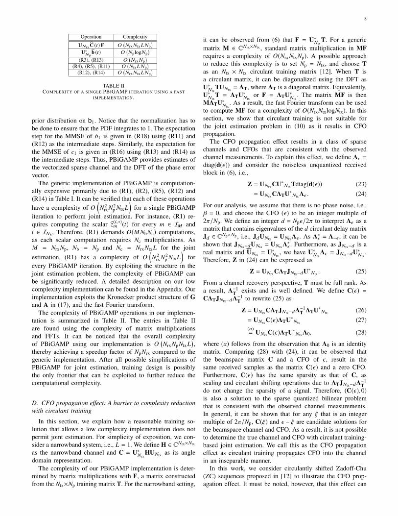
For a sequence of Np = 1024 pilots, our joint estimationalgorithm recovered the channel within acceptable limits witha probability greater than 0.95, at a SNR of 0 dB usingIID QPSK training. The number of outliers in this caseis determined by the phase-transition region of PBiGAMP[22]. It can be observed from Fig. 3 that the probabilityof successful recovery monotonically increases as a functionof the training length and quickly approaches 1. To ignore

-15 -12.5 -10 -7.5 -5 -2.5 0

x(dB)

0

0.1

0.2

0.3

0.4

0.5

0.6

0.7

0.8

0.9

1

Pr(NSE≤

x)

Np = 512Np = 1024Np = 2048Np = 4096

Fig. 3. The empirical CDF of the Normalized Squared Error of the channelestimate obtained using an IID QPSK training, at a SNR of 0 dB in a one-bitreceiver. The reconstruction performance in terms of the recovery probabilityand the mean monotonically improve with the number of pilots.

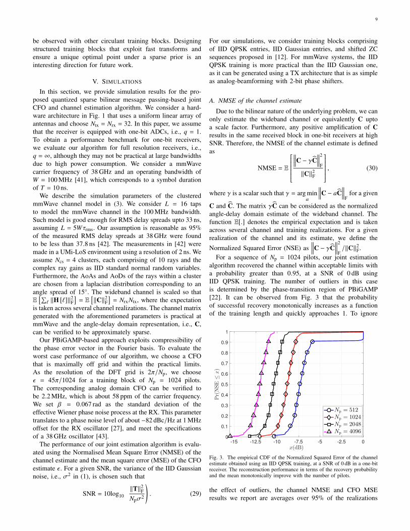
the effect of outliers, the channel NMSE and CFO MSEresults we report are averages over 95% of the realizations

10

for Np = 1024. In practice, the failure probability can belowered by increasing the training length or by designing aretransmission protocol that accounts for the failure. As seen in

512 1024 2048 3072 4096 5120

Number of pilots (Np)

-15

-14

-13

-12

-11

-10

-9

-8

-7

-6

-5

NMSE(dB)

IID QPSK, 1-bitIID QPSK, ∞-bit

Fig. 4. The NMSE of the channel estimate as a function of the traininglength, for an IID QPSK training at a SNR of 0 dB. The NMSE monotonicallydecreases with the training length for one-bit and full resolution receivers. Dueto the quantization noise in one-bit receivers, NMSE in the one-bit case ishigher than the full resolution one.

Fig. 4, the NMSE monotonically decreases with the number ofpilots. In practical wireless systems, the choice of the numberof pilots is determined by the channel coherence time [3].

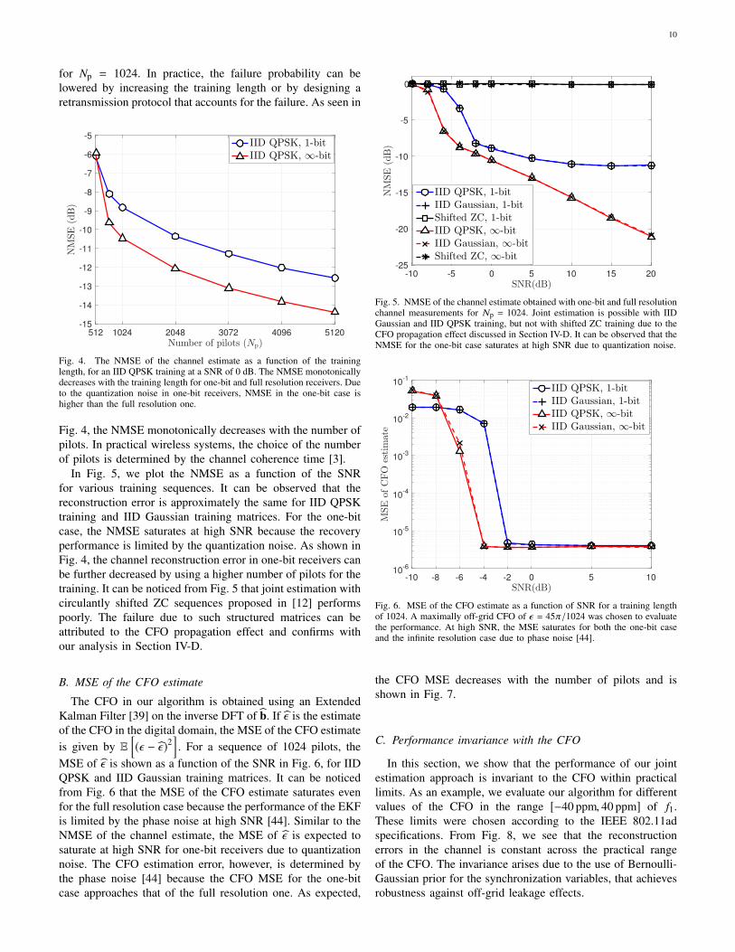
In Fig. 5, we plot the NMSE as a function of the SNRfor various training sequences. It can be observed that thereconstruction error is approximately the same for IID QPSKtraining and IID Gaussian training matrices. For the one-bitcase, the NMSE saturates at high SNR because the recoveryperformance is limited by the quantization noise. As shown inFig. 4, the channel reconstruction error in one-bit receivers canbe further decreased by using a higher number of pilots for thetraining. It can be noticed from Fig. 5 that joint estimation withcirculantly shifted ZC sequences proposed in [12] performspoorly. The failure due to such structured matrices can beattributed to the CFO propagation effect and confirms withour analysis in Section IV-D.

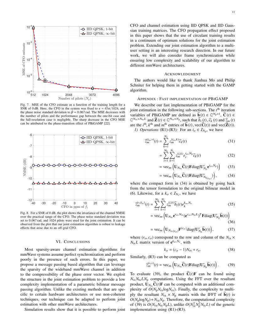
B. MSE of the CFO estimate

The CFO in our algorithm is obtained using an ExtendedKalman Filter [39] on the inverse DFT of b. If ε is the estimateof the CFO in the digital domain, the MSE of the CFO estimateis given by E

[(ε − ε)2

]. For a sequence of 1024 pilots, the

MSE of ε is shown as a function of the SNR in Fig. 6, for IIDQPSK and IID Gaussian training matrices. It can be noticedfrom Fig. 6 that the MSE of the CFO estimate saturates evenfor the full resolution case because the performance of the EKFis limited by the phase noise at high SNR [44]. Similar to theNMSE of the channel estimate, the MSE of ε is expected tosaturate at high SNR for one-bit receivers due to quantizationnoise. The CFO estimation error, however, is determined bythe phase noise [44] because the CFO MSE for the one-bitcase approaches that of the full resolution one. As expected,

-10 -5 0 5 10 15 20

SNR(dB)

-25

-20

-15

-10

-5

0

NMSE(dB)

IID QPSK, 1-bitIID Gaussian, 1-bitShifted ZC, 1-bitIID QPSK, ∞-bitIID Gaussian, ∞-bitShifted ZC, ∞-bit

Fig. 5. NMSE of the channel estimate obtained with one-bit and full resolutionchannel measurements for Np = 1024. Joint estimation is possible with IIDGaussian and IID QPSK training, but not with shifted ZC training due to theCFO propagation effect discussed in Section IV-D. It can be observed that theNMSE for the one-bit case saturates at high SNR due to quantization noise.

-10 -8 -6 -4 -2 0 5 10

SNR(dB)

10-6

10-5

10-4

10-3

10-2

10-1

MSEof

CFO

estimate

IID QPSK, 1-bitIID Gaussian, 1-bitIID QPSK, ∞-bitIID Gaussian, ∞-bit

Fig. 6. MSE of the CFO estimate as a function of SNR for a training lengthof 1024. A maximally off-grid CFO of ε = 45π/1024 was chosen to evaluatethe performance. At high SNR, the MSE saturates for both the one-bit caseand the infinite resolution case due to phase noise [44].

the CFO MSE decreases with the number of pilots and isshown in Fig. 7.

C. Performance invariance with the CFO

In this section, we show that the performance of our jointestimation approach is invariant to the CFO within practicallimits. As an example, we evaluate our algorithm for differentvalues of the CFO in the range [−40 ppm, 40 ppm] of f1.These limits were chosen according to the IEEE 802.11adspecifications. From Fig. 8, we see that the reconstructionerrors in the channel is constant across the practical rangeof the CFO. The invariance arises due to the use of Bernoulli-Gaussian prior for the synchronization variables, that achievesrobustness against off-grid leakage effects.

11

512 1024 2048 3072 4096

Number of pilots (Np)

10-6

10-5

10-4

10-3

10-2

MSEof

CFO

estimate

IID QPSK, 1-bitIID QPSK, ∞-bit

Fig. 7. MSE of the CFO estimate as a function of the training length for aSNR of 0 dB. Here, the CFO in the system was fixed to ε = 45π/1024, andthe phase noise standard deviation to β = 0.067 rad. The MSE decreases withthe number of pilots and the performance gap between the one-bit case andthe full-resolution case is negligible. The sharp decrease in the CFO MSEcan be attributed to the phase-transition effect of PBiGAMP [22].

-40 -30 -20 -10 0 10 20 30 40

CFO in ppm of f1

-12

-11

-10

-9

-8

-7

-6

NMSE(dB)

IID QPSK, 1-bitIID QPSK, ∞-bit

Fig. 8. For a SNR of 0 dB, the plot shows the invariance of the channel NMSEover the practical range of the CFO. The phase noise standard deviation wasset to 0.067 rad, and 1024 pilots were used for the joint estimation. It can beobserved from the plot that our joint estimation algorithm is robust to leakageeffects that arise due to an off-grid CFO.

VI. CONCLUSIONS

Most sparsity-aware channel estimation algorithms formmWave systems assume perfect synchronization and performpoorly in the presence of such errors. In this paper, wepropose a message passing based algorithm that can leveragethe sparsity of the wideband mmWave channel in additionto the compressibility of the phase error vector. We exploitthe structure in the joint estimation problem to provide a lowcomplexity implementation of a parametric bilinear messagepassing algorithm. Unlike the existing methods that are spe-cific to certain hardware architectures or use non-coherenttechniques, our technique can be adapted to perform jointestimation with other mmWave architectures.

Simulation results show that it is possible to perform joint

CFO and channel estimation using IID QPSK and IID Gaus-sian training matrices. The CFO propagation effect proposedin this paper shows that the use of circulant training resultsin a continuum of optimum solutions for the joint estimationproblem. Extending our joint estimation algorithm to a multi-user setting is an interesting research direction. In our futurework, we will also consider frame synchronization whileensuring low complexity and scalability of our algorithm todifferent mmWave architectures.

ACKNOWLEDGMENT

The authors would like to thank Jianhua Mo and PhilipSchniter for helping them in getting started with the GAMPalgorithm.

APPENDIX : FAST IMPLEMENTATION OF PBIGAMPWe describe our fast implementation of PBiGAMP for the

joint estimation in the following sub-sections. The tth iterationvariables of PBiGAMP are defined as b (t) ∈ CNp×1, C (t) ∈CNrx×NtxL and Z (t) ∈ CNrx×Np , such that bi (t) , ck (t) and zm (t)are the ith, k th and mth entries of b (t) , vec(C(t)) and vec(Z(t)).

1) Operations (R1)-(R3): For an io ∈ INp , we have

z(io,∗)m (t) =Nc∑k=1

z(io,k)m ck(t) (31)

=

Nb∑i=1

Nc∑k=1

z(i,k)m eio,Npi ck(t) (32)

= vecm(UNrxC(t)Fdiag(U∗Np

eio,Np )

)(33)

= vecm(UNrxC(t)Fdiag(U∗Np(io )

)

), (34)

where the compact form in (34) is obtained by going backfrom the tensor formulation to the original bilinear model in(6). Likewise, for a ko ∈ INc , we have

z(∗,ko )m (t) =Nb∑i=1

Nc∑k=1

z(i,k)m bi(t)eko,Nck

(35)

= vecm(UNrxero,Nrx (eco,NtxL)TFdiag(U∗Np

b(t)))(36)

= vecm(UNrx (ro )

F(co )diag(U∗Npb(t))

), (37)

where (ro, co) correspond to the row and column of the Nrx ×NtxL matrix version of eko,Nc , with

ko = (co − 1)Nrx + ro . (38)

Similarly, (R3) can be computed as

z(∗,∗)m (t) = vecm(UNrxC(t)Fdiag(U∗Np

b(t))). (39)

To evaluate (39), the product C(t)F can be found usingNrxNtxLNp computations. Using the FFT over the resultantproduct, UNrxC(t)F can be computed with an additional com-plexity of O(NpNrxlogNrx). Finally, the complexity to multi-ply the resultant Nrx × Np matrix with the IFFT of b(t) isO(NplogNp)+NrxNp. Therefore, the computational complexityof (39) is O(NrxNtxNpL), unlike O(N2

rxN2p NtxL) of the generic

implementation using (R1)-(R3).

12

2) Operations (R4) , (R5): It can be noticed from (34) thatz(i,∗)m (t) is invariant with respect to i and is given byz(i,∗)m (t)

= 1√Np

vecm(UNrxC(t)F

) . (40)

Using the invariance property in (40), a compact version ofthe first summand in (R4) can be expressed as

Np∑i=1

vbi

z(i,∗)m (t)2 = ∑Np

i=1 vbi

Npvecm

(UNrxC(t)F2) . (41)

For the second summand in (R4), it can be shown from (37)thatz(∗,ko )m (t)

= 1√

Nrxvecm

(F(co )diag(U∗Np

b(t)) ⊗ aNrx (0)

).

(42)

Furthermore, as co denotes the column number correspondingto ko (see (38)),

z(∗,k)m (t) is invariant ∀k ∈ IaNrx \ I(a−1)Nrx ,

where a ∈ INtxL . To use this invariance for efficient com-putation of the second summand in (R4), we define a rowvector µc(t) ∈ R1×NtxL containing the column-wise meancorresponding to Nrx × NtxL matrix version of

vck(t)

k∈INcas

µcn(t) =1

Nrx

∑vck (t)

k∈InNrx\I(n−1)Nrx

. (43)

With some algebraic manipulation, the second summand in(R4) can be simplified asNc∑k=1

vck (t)z(∗,k)m (t)

2= vecm[(µc(t)

Fdiag(U∗Npb(t))

2)⊗aNrx (0)].

(44)To simplify the computations involved in (R5), we expand thesummand using (17) as

Nb∑i=1

Nc∑k=1

vbi (t)vck (t)

z(i,k)m

2 = Nb∑i=1

Nc∑k=1

vbi (t)vck (t)

Gm,iAm,k

2(45)

=

∑Npi=1 v

bi (t)

Np

Nc∑k=1

vck (t)AT

k,m

2 , (46)

where (46) follows from (45) asGm,i

= 1√Np, ∀m, i. Besides,

as AT = F ⊗ UNrx , the entries ofAT

are invariant withinblocks of size Nrx × Nrx . With arguments similar to thesimplifications involved in the second summand of (R4), (R5)can be efficiently evaluated as

Nb∑i=1

Nc∑k=1

vbi (t)vck (t)

z(i,k)m

2 = ∑Npi=1 v

bi (t)

Np×

vecm[(µc(t) |F|2

)⊗ aNrx (0)

]. (47)

3) Operations (R11) , (R13): From (42), it can be observed

thatz(∗,k)m (t)

2 is fixed for m ∈ IaNrx \ I(a−1)Nrx and k ∈IbNrx \ I(b−1)Nrx , where a ∈ INp and b ∈ INtxL . The invariance

ofz(∗,k)m (t)

2 with respect to m and k arise because of the

Kronecker product with aNrx (0) and the column invariance in(38). To exploit this property in computing vr

k(t) of (R11),

we construct a vector µz(t) ∈ RNp×1 to contain the column-wise mean corresponding to the Nrx × Np matrix version ofvsm(t)

m∈INpNrx

, i.e.,

µzk(t) =

1Nrx

∑vsm(t)

m∈IkNrx\I(k−1)Nrx

. (48)

With the above definitions, a simplified version of(vrj (t)

)−1

in (R11) can be given asM∑m=1

vsm(t)z(∗,k)m

2 = veck[(Fdiag(U∗Np

b)2 µz(t)

)⊗ aNrx (0)

].

(49)From (40), we rewrite

(vqi (t)

)−1 in (R13) as(vqi (t)

)−1=

M∑m=1

vsmvecm(UNrxC(t)F

2)= vsvec

(UNrxC(t)F2) , ∀i ∈ INp .

4) Operations (R12) , (R14): We define F(t) =

Fdiag(U∗Np

b(t))

and consider the term in the secondsummand of (R12) for k = ko. From (37) and (38), we have

M∑m=1

sm(t )z(∗,ko )m (t)∗ =

M∑m=1

sm(t)vecm[UNrx(ro )F(t)

(co )]. (50)

With S(t) ∈ CNrx×Np defined such that sm(t) = vecm(S(t)

),

(50) can be expressed as,M∑m=1

sm(t )z(∗,ko )m (t)∗ =

⟨S(t),UNrx(ro )F(t)

(co )⟩

(51)

=(UNrx(ro )

)∗ S(t)(F(t)(co )

)∗(52)

= vecko(U∗Nrx

S(t)F(t)∗). (53)

The term in the third summand of (R12) can be given by

M∑m=1

vsm(t)Np∑i=1

vbi (t)z(i,k)m

2 = M∑m=1

vsm(t)

∑Npi=1 v

bi (t)

Am,k

2Np

=

(∑Npi=1 v

bi (t)

Np

)veck

(AT2 vs

).

Once again exploiting invariance withinAT

, we efficientlycompute the third summand in (R12) as

M∑m=1

vsm(t)Np∑i=1

vbi (t)z(i,k)m

2 = ∑Npi=1 v

bi (t)

Np×

veck[(|F|2 µz(t)

)⊗ aNrx (0)

]. (54)

The term in the second summand of (R14) can be rewrittenusing (34) as

M∑m=1

sm(t )z(i,∗)∗m =

⟨S(t),UNrxC(t)Fdiag(U∗Np(i)

)

⟩. (55)

13

For fast implementation of (55), we first compute the columnwise inner product between S(t) and UNrxC(t)F and then per-form a Fast Fourier Transform (FFT). We construct g ∈ CNp×1,

such that gk =⟨(

S(t))(k),(UNrxC(t)F

)(k)

⟩. Hence, the second

summand in (R14) simplifies toM∑m=1

sm(t )z(i,∗)∗m = veci

(UNpg

). (56)

The term in the third summand of (R14) can be expressed asM∑m=1

Nc∑k=1

vsm(t)vck (t)

z(i,k)m

2 = M∑m=1

Nc∑k=1

vsm(t)vck (t)

Gm,iAm,k

2(57)

=1

Np

M∑m=1

vsm(t)Nc∑k=1

vck (t)AT

k,m

2 .(58)

Using the compact form of∑Nc

k=1 vck(t)

ATk,m

2 from (47), werewrite (58) as

M∑m=1

Nc∑k=1

vsm(t)vck (t)

z(i,k)m

2 = 1Np

M∑m=1

(vsm(t)×

vecm[(µc(t) |F|2

)⊗ aNrx (0)

] ).

(59)

Furthermore, exploiting the kroenecker product with aNrx (0),we have

M∑m=1

Nc∑k=1

vsm(t)vck (t)

z(i,k)m

2 = NrxNp

µc(t) |F|2 µz(t). (60)

REFERENCES

[1] S. Rangan, T. S. Rappaport, and E. Erkip, “Millimeter-wave cellularwireless networks: Potentials and challenges,” in Proc. of the IEEE, vol.102, no. 3, pp. 366–385, 2014.

[2] A. Alkhateeb, J. Mo, N. Gonzalez Prelcic, and R. W. Heath Jr., “MIMOprecoding and combining solutions for millimeter wave systems,” IEEECommun. Mag., vol. 52, no. 12, pp. 122–131, 2014.

[3] R. W. Heath, Introduction to Wireless Digital Communication: A SignalProcessing Perspective. Pearson Education, 2017.

[4] R. W. Heath, N. Gonzalez-Prelcic, S. Rangan, W. Roh, and A. M.Sayeed, “An overview of signal processing techniques for millimeterwave MIMO systems,” IEEE J. Sel. Topics Signal Process., vol. 10,no. 3, pp. 436–453, 2016.

[5] E. J. Candes and M. B. Wakin, “An introduction to compressivesampling,” IEEE Signal Process. Mag., vol. 25, no. 2, pp. 21–30, 2008.

[6] P. T. Boufounos and R. G. Baraniuk, “One bit compressive sensing,” inProc. of the IEEE 42nd Annual Conf. on Inform. Sciences and Systems,2008., 2008, pp. 16–21.

[7] Z. Marzi, D. Ramasamy, and U. Madhow, “Compressive channel esti-mation and tracking for large arrays in mm-wave picocells,” IEEE J.Sel. Topics Signal Process., vol. 10, no. 3, pp. 514–527, 2016.

[8] A. Alkhateeb, O. El Ayach, G. Leus, and R. W. Heath, “Channelestimation and hybrid precoding for millimeter wave cellular systems,”IEEE J. Sel. Topics Signal Process., vol. 8, no. 5, pp. 831–846, 2014.

[9] J. Mo, P. Schniter, N. G. Prelcic, and R. W. Heath, “Channel estimationin millimeter wave MIMO systems with one-bit quantization,” in Proc.of the Asilomar Conf. on Signals, Systems and Computers, 2014, pp.957–961.

[10] D. L. Donoho, A. Maleki, and A. Montanari, “Message-passing al-gorithms for compressed sensing,” Proc. of the National Academy ofSciences, vol. 106, no. 45, pp. 18 914–18 919, 2009.

[11] J. P. Vila and P. Schniter, “Expectation-maximization Gaussian-mixtureapproximate message passing,” IEEE Trans. on Signal Process., vol. 61,no. 19, pp. 4658–4672, 2013.

[12] J. Mo, P. Schniter, and R. W. Heath Jr., “Channel estimation inbroadband millimeter wave MIMO systems with few-bit ADCs,” IEEETrans. on Signal Process., 2017.

[13] H. Yan and D. Cabric, “Compressive sensing based initial beamformingtraining for massive MIMO millimeter-wave systems,” in Proc. of theIEEE Global Conf. on Signal and Info. Process. (GlobalSIP), 2016, pp.620–624.

[14] N. J. Myers and R. W. Heath Jr., “A compressive channel estimationtechnique robust to synchronization impairments,” in Proc. of the 18thIEEE Intl. Workshop on Signal Process. Adv. in Wireless Commun.(SPAWC), 2017, pp. 1–5.

[15] J. Chen, Y.-C. Wu, S. Ma, and T.-S. Ng, “Joint CFO and channelestimation for multiuser MIMO-OFDM systems with optimal trainingsequences,” IEEE Trans. on Signal Process., vol. 56, no. 8, pp. 4008–4019, 2008.

[16] W. Zhang, Q. Yin, W. Wang, and F. Gao, “One-shot blind CFO andchannel estimation for OFDM with multi-antenna receiver,” IEEE Trans.on Signal Process., vol. 62, no. 15, pp. 3799–3808, 2014.

[17] O. Abari, H. Hassanieh, M. Rodreguez, and D. Katabi, “Millimeter wavecommunications: From point-to-point links to agile network connec-tions,” in Proc. of the ACM Workshop on Hot Topics in Networks, 2016,pp. 169–175.

[18] M. E. Rasekh, Z. Marzi, Y. Zhu, U. Madhow, and H. Zheng, “Nonco-herent mmwave path tracking,” in Proc. of the 18th ACM Intl. Workshopon Mobile Computing Systems and Applications, 2017, pp. 13–18.

[19] N. J. Myers and R. W. Heath Jr., “Joint CFO and channel estimationin millimeter wave systems with one-bit ADCs,” in Proc. of the 7thIEEE Intl. Workshop on Comput. Adv. in Multi-Sensor Adapt. Process.(CAMSAP), 2017, pp. 1–5.

[20] N. D. Sidiropoulos, L. De Lathauwer, X. Fu, K. Huang, E. E. Papalex-akis, and C. Faloutsos, “Tensor decomposition for signal processing andmachine learning,” IEEE Trans. on Signal Process., vol. 65, no. 13, pp.3551–3582.

[21] E. J. Candes, T. Strohmer, and V. Voroninski, “Phaselift: Exact andstable signal recovery from magnitude measurements via convex pro-gramming,” Commun. on Pure and Applied Mathematics, vol. 66, no. 8,pp. 1241–1274, 2013.

[22] J. T. Parker and P. Schniter, “Parametric bilinear generalized approximatemessage passing,” IEEE J. Sel. Topics Signal Process., vol. 10, no. 4,pp. 795–808, 2016.

[23] L. He, J. Wang, and J. Song, “Spatial modulation for more spatialmultiplexing: RF-chain-limited generalized spatial modulation aidedmm-wave MIMO with hybrid precoding,” IEEE Trans. on Commun.,vol. 66, no. 3, pp. 986–998, 2018.

[24] W. Deng, T. Siriburanon, A. Musa, K. Okada, and A. Matsuzawa, “Asub-harmonic injection-locked quadrature frequency synthesizer withfrequency calibration scheme for millimeter-wave TDD transceivers,”IEEE J. of Solid-State Circuits, vol. 48, no. 7, pp. 1710–1720, 2013.

[25] K.-H. Tsai, J.-H. Wu, and S.-I. Liu, “A digitally calibrated 64.3–66.2GHz phase-locked loop,” in IEEE Radio Frequency Integrated CircuitsSymposium, 2008, pp. 307–310.

[26] D. Petrovic, W. Rave, and G. Fettweis, “Effects of phase noise on OFDMsystems with and without PLL: Characterization and compensation,”IEEE Trans. on Commun., vol. 55, no. 8, pp. 1607–1616, 2007.

[27] A. Demir, A. Mehrotra, and J. Roychowdhury, “Phase noise in oscilla-tors: A unifying theory and numerical methods for characterization,”IEEE Trans. on Circuits and Systems I: Fundamental Theory andApplications, vol. 47, no. 5, pp. 655–674, 2000.

[28] M. R. Khanzadi, R. Krishnan, J. Soder, and T. Eriksson, “On the capacityof the wiener phase-noise channel: Bounds and capacity achievingdistributions,” IEEE Transactions on Communications, vol. 63, no. 11,pp. 4174–4184, 2015.

[29] K. Venugopal, A. Alkhateeb, N. G. Prelcic, and R. W. Heath, “Channelestimation for hybrid architecture-based wideband millimeter wavesystems,” IEEE Journal on Selected Areas in Commun., vol. 35, no. 9,pp. 1996–2009, 2017.

[30] J. Wang, “Beam codebook based beamforming protocol for multi-Gbpsmillimeter-wave WPAN systems,” IEEE Journal on Selected Areas inCommun., vol. 27, no. 8, 2009.

[31] M. F. Duarte and R. G. Baraniuk, “Spectral compressive sensing,”Applied and Computational Harmonic Analysis, vol. 35, no. 1, pp. 111–129, 2013.

14

[32] F. Pancaldi, G. M. Vitetta, R. Kalbasi, N. Al-Dhahir, M. Uysal, andH. Mheidat, “Single-carrier frequency domain equalization,” IEEE Sig-nal Process. Mag., vol. 25, no. 5, 2008.

[33] V. Syrjala and M. Valkama, “Receiver DSP for OFDM systems impairedby transmitter and receiver phase noise,” in Proc. of the IEEE Intl. Conf.on Commun. (ICC), 2011, pp. 1–6.

[34] S. Ling and T. Strohmer, “Self-calibration and biconvex compressivesensing,” Inverse Problems, vol. 31, no. 11, p. 115002, 2015.

[35] S. Rangan, “Generalized approximate message passing for estimationwith random linear mixing,” in Proc. of the IEEE Intl. Symposium onInform. Theory, 2011, pp. 2168–2172.

[36] S. M. Kay, Fundamentals of statistical signal processing. Prentice HallPTR, 1993.

[37] F. R. Kschischang, B. J. Frey, and H.-A. Loeliger, “Factor graphs andthe sum-product algorithm,” IEEE Trans. on Inform. Theory, vol. 47,no. 2, pp. 498–519, 2001.

[38] J. Vila and P. Schniter, “Expectation-maximization bernoulli-gaussianapproximate message passing,” in Proc. of the Asilomar Conf. onSignals, Systems and Computers, 2011, pp. 799–803.

[39] R. E. Kalman, “A new approach to linear filtering and predictionproblems,” vol. 82, no. 1, 1960, pp. 35–45.

[40] C.-K. Wen, C.-J. Wang, S. Jin, K.-K. Wong, and P. Ting, “Bayes-optimaljoint channel-and-data estimation for massive MIMO with low-precisionADCs,” IEEE Trans. on Signal Process., vol. 64, no. 10, pp. 2541–2556.

[41] F. B. Mismar and B. L. Evans, “Machine learning approach to esti-mating mmWave signal measurements during handover,” arXiv preprintarXiv:1710.01879, 2017.

[42] Aalto Univ., AT & T, BUPT, CMCC, Ericsson, Huawei, Intel, KTCorporation, Nokia, NTT DOCOMO, New York Univ., Qualcomm,Samsung, Univ. of Bristol, and Univ. of Southern California, “5Gchannel model for bands up to 100 GHz (v2.3), Tech. Rep.” http://www.5gworkshops.com/5gcm.html, 2016, [Online].

[43] “MMIC Voltage Controlled Oscillator,” http://www.tlcprecision.com/Data%20Sheets/TLCO01981.pdf, 2013, [Online].

[44] O. H. Salim, A. A. Nasir, H. Mehrpouyan, W. Xiang, S. Durrani, andR. A. Kennedy, “Channel, phase noise, and frequency offset in OFDMsystems: Joint estimation, data detection, and hybrid Cramer-Rao lowerbound,” IEEE Trans. on Commun., vol. 62, no. 9, pp. 3311–3325, 2014.

Nitin Jonathan Myers received the B.Tech andM.Tech degrees in Electrical Engineering from theIndian Institute of Technology (IIT) Madras in 2016.He is currently pursuing the Ph.D. degree at theUniversity of Texas at Austin. His research interestslie in the areas of wireless communications andsignal processing. Mr. Myers received the 2018 and2019 Electrical and Computer Engineering researchawards from the Cockrell School of Engineering atThe University of Texas at Austin, and the UniversityGraduate Continuing Fellowship from 2019 to 2020.

During his undergraduate days at IIT Madras, he received the DAAD WISEscholarship in 2014, and the Institute Silver Medal in 2016.

Robert W. Heath Jr. (S’96 - M’01 - SM’06- F’11) received the B.S. and M.S. degrees fromthe University of Virginia, Charlottesville, VA, in1996 and 1997 respectively, and the Ph.D. fromStanford University, Stanford, CA, in 2002, all inelectrical engineering. From 1998 to 2001, he was aSenior Member of the Technical Staff then a SeniorConsultant at Iospan Wireless Inc, San Jose, CAwhere he worked on the design and implementationof the physical and link layers of the first commercialMIMO-OFDM communication system. Since Jan-

uary 2002, he has been with the Department of Electrical and ComputerEngineering at The University of Texas at Austin where he is a Cullen Trustfor Higher Education Endowed Professor, and is a Member of the WirelessNetworking and Communications Group. He is also President and CEO ofMIMO Wireless Inc. He authored Introduction to Wireless Digital Commu-nication (Prentice Hall, 2017) and Digital Wireless Communication: PhysicalLayer Exploration Lab Using the NI USRP’ (National Technology and SciencePress, 2012), and co-authored Millimeter Wave Wireless Communications’(Prentice Hall, 2014).

Dr. Heath has been a co-author of sixteen award winning conferenceand journal papers including the 2010 and 2013 EURASIP Journal onWireless Communications and Networking best paper awards, the 2012 SignalProcessing Magazine best paper award, a 2013 Signal Processing Society bestpaper award, 2014 EURASIP Journal on Advances in Signal Processing bestpaper award, the 2014 and 2017 Journal of Communications and Networksbest paper awards, the 2016 IEEE Communications Society Fred W. EllersickPrize, the 2016 IEEE Communications and Information Theory Societies JointPaper Award, and the 2017 Marconi Prize Paper Award. He received the 2017EURASIP Technical Achievement award. He was a distinguished lecturer inthe IEEE Signal Processing Society and is an ISI Highly Cited Researcher.In 2017, he was selected as a Fellow of the National Academy of Inventors.He is also an elected member of the Board of Governors for the IEEE SignalProcessing Society, a licensed Amateur Radio Operator, a Private Pilot, aregistered Professional Engineer in Texas. He is currently Editor-in-Chief ofIEEE Signal Processing Magazine.