Embed Size (px)
Citation preview
arX
iv:1
509.
0905
9v2
[cs.
IT]
4 Ja
n 20
161
Message-Passing Receiver for Joint Channel
Estimation and Decoding in 3D Massive
MIMO-OFDM Systems
Sheng Wu,Member, IEEE, Linling Kuang,Member, IEEE,
Zuyao Ni, Defeng (David) Huang,Senior Member, IEEE,
Qinghua Guo,Member, IEEE, and Jianhua Lu,Fellow, IEEE
Abstract
In this paper, we address the message-passing receiver design for the 3D massive MIMO-OFDM
systems. With the aid of the central limit argument and Taylor-series approximation, a computationally
efficient receiver that performs joint channel estimation and decoding is devised by the framework of
expectation propagation. Specially, the local belief defined at the channel transition function is expanded
up to the second order with Wirtinger calculus, to transformthe messages sent by the channel transition
function to a tractable form. As a result, the channel impulse response (CIR) between each pair of
antennas is estimated by Gaussian message passing. In addition, a variational expectation-maximization
(EM)-based method is derived to learn the channel power-delay-profile (PDP). The proposed joint
This work was partially supported by the National Nature Science Foundation of China (Grant Nos. 91338101, 61231011,
and 91438206), the National Basic Research Program of China(Grant No. 2013CB329001), and Tsinghua University Initiative
Scientific Research Program (Grant No. 20131089219).
Sheng Wu, Linling Kuang and Zuyao Ni are with the Tsinghua Space Center, Tsinghua University, China (e-mail:
{thuraya, kll, nzy}@tsinghua.edu.cn).
Defeng (David) Huang is with the School of Electrical, Electronic and Computer Engineering, The University of Western
Australia, Australia (e-mail: [email protected]).
Q. Guo is with the School of Electrical, Computer and Telecommunications Engineering, University of Wollongong, Australia,
and is also with the School of Electrical, Electronic and Computer Engineering, The University of Western Australia, Australia
(e-mail: [email protected]).
Jianhua Lu is with the Department of Electronic Engineering, Tsinghua University, China (e-mail:
2
algorithm is assessed in 3D massive MIMO systems with spatially correlated channels, and the empirical
results corroborate its superiority in terms of performance and complexity.
Index Terms
Expectation Propagation, Joint Channel Estimation and Decoding, 3D Massive MIMO, Message
Passing, OFDM.
I. INTRODUCTION
Recently, massive multiple-input multiple-output (MIMO)systems with tens to hundreds of
antennas at the base-station (BS) have gained significant attention [1]–[4]. It has been proved that
massive MIMO systems can scale down transmit power as well asincrease spectrum efficiency
by orders of magnitude [2]. One of the tasks in massive MIMO systems is estimating the
channel impulse response (CIR) for each transmit-receive link, since high data rates and energy
efficiency can only be achieved when CIR is known [5]. In contrast to the conventional MIMO
systems employing a small number of antennas, there are a large number of channels need to
be estimated. The pilot overhead required for channel estimation is proportional to the number
of transmit antennas, which can be excessive in massive MIMOsystems [6]. In the meantime,
the available resources for training are restricted by the channel coherence time. On the other
hand, the energy consumption by baseband processing grows with the number of antennas,
which may obliterate the advantage of massive MIMO systems in energy efficiency. Thus, low-
complexity channel estimation with high accuracy and reduced overhead is critical to massive
MIMO systems.
Iterative receivers that jointly estimate the channel coefficients and detect the data symbols
are able to provide more accurate channel estimation with less training overhead [7]–[12].
Factor graph and sum-product algorithm (SPA) [13] have beenused as a unified framework for
iterative joint data detection, channel estimation, interference cancellation, and decoding [14],
[15]. However, exact SPA for joint channel estimation and decoding is computationally infeasible.
To overcome this problem, various message-passing algorithms based on approximate inference
have been proposed [8], [16]–[23]. In existing approaches,the message passing strategies include
loopy belief propagation (LBP) [8], [16], [19]–[21], variational methods [17], [23], [24], and a
hybrid of both [18], [22].
3
LBP has a high complexity when applied to graphical models that involve both discrete and
continuous random variables. This has been addressed by merging the SPA with the expectation-
maximization (EM) algorithm [19] or approximating the messages of SPA with Gaussian mes-
sages [8], [19], [20], [25]. Variational inference methodshave been applied to MIMO receivers
for joint detection, channel estimation, and decoding [17]. In [18], Riegler et al. derived a
generic message-passing algorithm that merges belief propagation (BP) with the mean-field
(MF) approximation (BP-MF), and applied it to joint channelestimation and decoding in single-
input single-output orthogonal frequency division multiplex (OFDM) systems and MIMO-OFDM
systems [18], [22], [26]. The BP-MF has to learn the noise precision to take into account the
residual interference from other users even when the noise power is known [27], [28], as the
channel transition functions are incorporated into the MF part [18], [22], [26]. Otherwise, the
uncertainty of residual interference is completely ignored, and the likelihood function associated
with the messages extracted from observations tends to overwhelm the a priori probability.
Besides, the BP-MF requires high computational complexityas large matrices need to be inverted
to estimate channel frequency response (CFR) [18], and thereby it is only feasible in the case
of a few antennas and subcarriers. We note that there is a low-complexity version of the BP-MF
algorithm proposed in [29], but its performance is inferior. The degraded performance may be
due to the unrealistic assumption that groups of contiguouschannel weights in frequency-domain
obey a Markov model.
To achieve joint channel estimation and decoding for massive MIMO systems using OFDM
modulation in frequency-selective channels, the receiverneeds to complete three tasks: decou-
pling frequency-domain channel coefficients and data symbols from noisy observations, decoding,
and channel estimation. Via central-limit theorem and moment matching, an approximate BP has
been derived in [8], [16] and [21]. Despite its superior performance, the approximate BP bears
a heavy computation burden: it needs to take a large number ofmoment-matching operations,
each being highly complicated. In this paper, we use the framework of expectation propagation
(EP) [30] to derive an efficient message-passing algorithm.Specifically, at the channel transition
functions, we use the central-limit theorem to efficiently obtain the beliefs of frequency-domain
channel coefficients and the beliefs of data symbols, and then employ a quadratic approximation
to project them into the Gaussian family. In the meantime, the expectation propagation principle
is applied to the symbol-variable nodes. As the beliefs of frequency-domain channel coefficients
4
are now in the form of Gaussian family, a Gaussian message passing based estimator [31]
can be employed, which exploits the fact that the CFR is the Fourier transformation of the
CIR. Furthermore, using the beliefs of time-domain channeltaps, the unknown power-delay-
profile (PDP) can be learned by variational expectation maximization. We note that Parkeret al.
applied central-limit theorem and Taylor-series approximations to formulate a bilinear generalized
approximate message-passing algorithm for the SPA in the high dimensional limit [32], but its
scope is different from that of this work.
The proposed scheme of joint channel estimation and decoding is assessed in 3D massive
MIMO systems with spatially correlated channels. Experiments show that its performance is
within 1 dB of the known-channel bound in both a64× 8 MIMO system and a16× 8 MIMO
system, and outperforms the performance of BP-MF by 0.4 dB inthe 16 × 8 MIMO system,
the low-complexity version of BP-MF by 1.2 dB in the64× 8 MIMO system and 1.6 dB in the
16× 8 MIMO system. On the other hand, the complexity of the proposed algorithm is a small
percentage of that of BP-MF and13
of that of the low-complexity version of BP-MF.
The remainder of this paper is organized as follows. The system model is described in Section
II. In Section III the message passing for joint detection and decoding is detailed. Complexity
comparisons are shown in Section IV, and numerical results are provided in Section V, followed
by conclusions in Section VI.
Notation: Lowercase letters (e.g.,x) denote scalars, bold lowercase letters (e.g.,x) denote
column vectors, and bold uppercase letters (e.g.,X) denote matrices. The superscripts(·)T, (·)H
and (·)∗ denote the transpose operation, Hermitian transpose operation, and complex conjugate
operation, respectively. Also,diag{x} denotes a square diagonal matrix with the elements of
vector x on the main diagonal;X ⊗ Y denotes Kronecker product ofX and Y ; I de-
notes an identity matrix; andln(·) denotes the natural logarithm. Furthermore,NC(x; x, νx) =
(πνx)−1 exp(− |x− x|2 /νx) denotes the Gaussian probability density function (PDF) ofx with
meanx and varianceνx; andGam(γ;α, β) = βαγα−1 exp(−βγ)/Γ(α) denotes the Gamma PDF
of γ with shape parameterα and rate parameterβ, whereΓ(·) is the gamma function. Finally,
∝ denotes equality up to a constant scale factor;x\xtnk denotes all elements inx but xtnk; and
Ep(x){·} denotes expectation with respect to distributionp(x).
5
II. SYSTEM MODEL
We consider the uplink of a massive MIMO system whereN single antenna users communicate
with a BS simultaneously. The BS employs a uniform planar array (UPA) consisting ofM =
(D×W ) ≫ N antennas distributed acrossD rows andW columns. Frequency-selective block-
fading channels are assumed, and OFDM is employed to combat multipath interference.
A. Channel Model
The CIR between thenth user and themth receive antenna is denoted byhmn· = [hmn1 · · ·hmnL]T,
wherehmnl is thelth path gain andL is the maximum channel spread. Leth·nl = [h1nl · · ·hMnl]T
denote gain vector of thelth paths between usern and all theM receive antennas at the BS.
Due to close antenna spacing at the BS, we can assume that theM CIRs between the usern
and all theM receive antennas at the BS follow an identical PDP{E{|hmnl|2} , αnl, ∀m}.
We can also assume that the transmit antennas from differentusers are spatially uncorrelated.
Accordingly, the Kronecker spatial fading correlation model for the gain vectorh·nl is given by
[33]
h·nl = R12nlh
iidnl , (1)
whereRnl ∈ CM×M denotes the receive correlation matrix, andhiidnl ∈ CM×1 denotes independent
complex Gaussian matrix with zero mean and covariance matrix αnlI. A ray-based 3D channel
model from [34] is employed, and the receive correlation matrix Rnl is approximated by
Rnl ≈ Raznl ⊗Rel
nl, (2)
whereRaznl ∈ RW×W and Rel
nl ∈ RD×D are the correlation matrices in azimuth and elevation
directions, respectively, and are defined by [34]
[Raznl]ww′ =
1√bexp
(
−a2cos2(θaznl)− 2jccos(θaznl) + νaznl (csin(θ
aznl))
2
2b
)
, (3)
[Relnl]dd′ = exp
(
2jπλdel (d′ − d) cos
(θelnl)− νelnl
(πdel (d′ − d) sin
(θelnl))2
λ2
)
, (4)
in terms of
a =2πdaz
λ
√
νelnl (w′ − w) cos
(θelnl), (5)
b = νaznla2sin2 (θaznl) + 1, (6)
6
c =2πdaz
λ(w′ − w) sin
(θelnl), (7)
whereλ is the carrier wavelength,θaznl and θelnl are the mean of horizontal angle-of-departure
(AoD) and the mean of vertical AoD, respectively;νaznl and νelnl are the variance of horizontal
AoD and the variance of vertical AoD, respectively;del anddaz are the vertical antenna spacing
and the horizontal antenna spacing, respectively.
B. Signal Model
For thenth user, the information bitsbn are encoded and interleaved, yielding a sequence
of coded bitscn. Then eachQ bits in cn are mapped to one modulation symbolxdn, which
is chosen from a2Q-ary constellation setA, i.e., |A| = 2Q. The data symbolsxdn are then
multiplexed with pilot symbolsxpn, forming the transmitted symbols sequencexn. Pilot and
data symbols are arranged in an OFDM frame ofT OFDM symbols, each consisting ofK
subcarriers. Specifically, the frequency-domain symbols in the tth OFDM symbols transmitted
by thenth user are denoted byxtn· = [xtn1, . . . , xtnK ]T, wherextnk ∈ A denotes the symbol
transmitted at thekth subcarrier. In each OFDM frame, there areKp ≤ K pilot subcarriers in
one selected OFDM symbol and the pilot subcarriers are spaced uniformly. The set of pilot-
subcarriers of usern is denoted byPn = {(t, k) : xtnk is a pilot symbol}, |Pn| = Kp, and the set
of data-subcarriers is denoted byD =⋃
nPn. To maintain the orthogonality between the pilot
sequences sent by different user, pilots symbols can be frequency division multiplexing, time
division multiplexing, code division multiplexing or hybrid of them. For simplicity, the sets of
pilot-subcarriers belong to different users are set to be mutually exclusive, i.e.,⋂
nPn = ∅, and
only one user actually transmits a pilot symbol at a given subcarrier, whereas the other users
transmit zero-symbol at this subcarrier [35], i.e.,xtn′k = 0, ∀n′ 6= n, if (t, k) ∈ Pn. To modulate
the OFDM symbol, aK-point inverse discrete Fourier transform (IDFT) is applied to the symbol
sequencextn· and then a cyclic prefix (CP) is added before transmission.
At the receiver, the CP is removed first and then the received signal from each receive antenna
is converted into frequency domain through aK-point discrete Fourier transform (DFT). It is
assumed that theN transmitters and the receiver are synchronized and the duration of the cyclic
prefix is larger than the maximum delays. And then the received signal during the interval of
7
the tth OFDM symbol can be written as
ytmk =∑
n
wmnkxtnk +tmk, (8)
whereytmk denotes the received signal at thekth subcarrier on themth receive antenna, tmk
denotes a circularly symmetric complex noise with zero meanand the variance ofσ2, andwmnk
denotes the CFR at thekth subcarrier between thenth user and themth receive antenna, which
is given by
wmnk =L∑
l=1
hmnlexp
(
−j2πlkK
)
. (9)
The received signal for a frame ofT OFDM symbols can be recast in a matrix-vector form as
y =N∑
n=1
W nxn + = Wx+, (10)
wherey = [yT1 · · ·yT
M ]T with ym = [y1m1 · · · y1mK · · · yTm1 · · · yTmK ]T denoting the received
signal at themth receive antenna forT OFDM symbols,W n = [IT ⊗ diag{w1n·} · · ·IT ⊗diag{wMn·}]T with wmn· = [wmn1 · · ·wmnK ]T denoting the CFR from thenth user to themth
antenna,W = [W 1 · · ·WN ], x = [xT1 · · ·xT
N ]T with xn = [x1n1 · · ·x1nK · · ·xTn1 · · ·xTnK ]T
denoting the symbols transmitted by thenth user, and = [T1 · · ·T
M ]T with m =
[1m1 · · ·1mK · · ·Tm1 · · ·TmK ]T denoting the noise signal at themth receive antenna.
C. Factor Graph Representation of the Massive MIMO-OFDM Systems
Our goal is to infer the information bits{bn} from the observationsy with the known pilot
symbols{xpn}. In particular, we aim to achieve the minimum bit error rate (BER) utilizing the
maximuma posteriori marginal criterion, i.e.,
bnι = arg maxbnι∈{0,1}
p (bnι | y) , (11)
where bnι denotes theιth information bit inbn, and thea posteriori probability p(bnι | y) is
given by
p (bnι | y) ∝∑
b\bnι,c,x
ˆ
H,W
p (b, c,x,y,W ,H) . (12)
Sinceb � c � x � y is a Markov chain and the CFR matrixW only depends on the CIR
matrix H, the joint probabilityp(b, c,x,y,W ,H) can be factorized into
p (b, c,x,y,W ,H) = p (b) p (c | b) p (x | c) p (y | W ,x) p (H ,W ) . (13)
8
The conditional probabilityp(x | c) in (13) can be factorized into
p (x | c) =∏
t
p (xt | ct) =∏
t,n,k
p (xtnk | ctnk) , (14)
wherect , {ctnk, ∀n, k}, xt , {xtnk, ∀n, k}, p(xtnk | ctnk) = δ(ϕ(ctnk) − xtnk) denotes the
deterministic mappingxtnk = ϕ(ctnk), ϕ(ctnk) is the mapping function andδ(·) is the Kronecker
delta function. In practice, the receive correlation matrices{Rnl} are unknown, so we impose
a conditional independent structure on thea priori probability ofH, i.e.,
p (H | γ) =∏
n,l
p (h·nl | γnl) , (15)
p (h·nl | γnl) =∏
m
p (hmnl | γnl) , (16)
p (hmnl | γnl) = NC
(hmnl; γ
−1nl
), (17)
p (γnl) = Gam(γnl; 0, 0), (18)
whereγ , {γnl}, andγnl is the inversion of PDP to be learned. As the CFRwmn· is the Fourier
transformations of the CIRhmn·, i.e., wmn· = Φhmn·, ∀m, ∀n, then the conditional probability
p(W | H) reads
p(W | H) =∏
m,n
p(wmn· | hmn·) =∏
m,n,k
δ
(
wmnk −∑
l
φklhmnl
)
, (19)
whereΦ ∈ CK×L denotes the DFT weighting matrix, andφkl denotes the entry in thekth row
and lth column ofΦ. The channel transition functionp(y | W ,x) is factorized into
p(y | W ,x) =∏
t,m,k
ftmk (xt·k,wm·k) , (20)
wherext·k , [xt1k · · ·xtNk]T, wm·k , [wm1k · · ·wmNk]T, and
ftmk (xt·k,wm·k) = NC
(
ytmk;∑
n
wmnkxmnk, σ2
)
. (21)
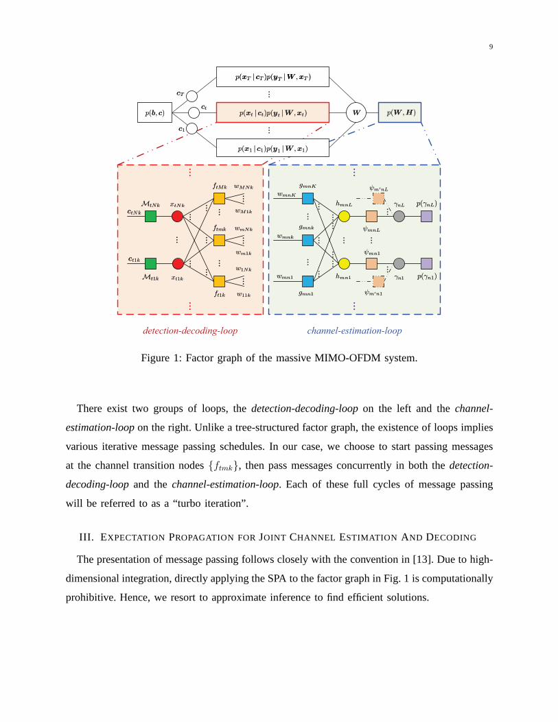
The probabilistic structure defined by the factorizations (13)-(20) can be represented by the
factor graph, as depicted in Fig. 1. In this factor graph, mapping constraintδ(ϕ(ctnk) − xtnk)
appears as a function nodeMtnk, the mixing constraintδ(wmnk−∑
l φklhmnl) appears as function
nodegmnk, and thea prior distributionψ(hmnl, γnl) appears as function nodeψmnl.
9
wmn1wmn1
wmnKwmnK
wmnkwmnk
gmnKgmnK
gmnkgmnk
hmn1hmn1
ÃmnLÃmnL
Ãmn1Ãmn1
hmnLhmnL
p(b; c)p(b; c) p(xt j ct)p(yt jW ;xt)p(xt j ct)p(yt jW ;xt)
p(x1 j c1)p(y1jW ; x1)p(x1 j c1)p(y1jW ; x1)
p(W ;H)p(W ;H)ctct
cTcT
WW
c1c1
ctNkctNk
ct1kct1k
MtNkMtNk
Mt1kMt1k xt1kxt1k
xtNkxtNk
ftmkftmk
ftMkftMk
w11kw11k
w1Nkw1Nk
wm1kwm1k
wmNkwmNk
wM1kwM1k
wMNkwMNk
ft1kft1k
detection-decoding-loop channel-estimation-loop
gmn1gmn1
°nL°nL
°n1°n1
p(°nL)p(°nL)
p(°n1)p(°n1)
Ãm0nLÃm0nL
Ãm0n1Ãm0n1
Figure 1: Factor graph of the massive MIMO-OFDM system.
There exist two groups of loops, thedetection-decoding-loop on the left and thechannel-
estimation-loop on the right. Unlike a tree-structured factor graph, the existence of loops implies
various iterative message passing schedules. In our case, we choose to start passing messages
at the channel transition nodes{ftmk}, then pass messages concurrently in both thedetection-
decoding-loop and thechannel-estimation-loop. Each of these full cycles of message passing
will be referred to as a “turbo iteration”.
III. EXPECTATION PROPAGATION FORJOINT CHANNEL ESTIMATION AND DECODING
The presentation of message passing follows closely with the convention in [13]. Due to high-
dimensional integration, directly applying the SPA to the factor graph in Fig. 1 is computationally
prohibitive. Hence, we resort to approximate inference to find efficient solutions.
10
A. Message Updating in Detection-Decoding-Loop
Note that, to update the outgoing messages from the channel transition nodeftmk, the received
signal shown in (8) can be rewritten as
ytmk = wmnkxtnk +∑
n′ 6=n
wmn′kxtn′k +tmk, ∀n. (22)
The interference term∑
n′ 6=nwmn′kxtn′k + tmk in (22) is considered as a Gaussian variable
[32], [36], and thenytmk −(∑
n′ 6=nwmn′kxtn′k + tmk
)is also a Gaussian variable with the
meanz(i)ftmk�xtnkand varianceτ (i)ftmk�xtnk
given by
z(i)ftmk�xtnk
= ytmk −∑
n′ 6=n
w(i−1)wmn′k�ftmk
x(i−1)xtn′k�ftmk
, (23)
τ(i)ftmk�xtnk
= σ2 +
∑
n′ 6=n
(∣∣w
(i−1)wmn′k�ftmk
∣∣2ν(i−1)xtn′k�ftmk
+ν(i−1)wmn′k�ftmk
∣∣x
(i−1)xtn′k�ftmk
∣∣2 + ν
(i−1)wmn′k�ftmk
ν(i−1)xtn′k�ftmk
)
, (24)
wherex(i−1)xtnk�ftmk
andν(i−1)xtnk�ftmk
denote the mean and variance of variablextnk with respect to the
messageµ(i−1)xtnk�ftmk
(xtnk); w(i−1)wmnk�ftmk
andν(i−1)wmnk�ftmk
denote the mean and variance of variable
wmnk with respect to the messageµ(i−1)wmnk�ftmk
(wmnk). From the model shown in (22)-(24), the
channel transition functionftmk at theith turbo iteration can be viewed as
f(i)tmk(wmnk, xtnk) = NC
(
wmnkxtnk; z(i)ftmk�xtnk
, τ(i)ftmk�xtnk
)
, ∀n (25)
Consequently, the messageµ(i)ftmk�xtnk
(xtnk) is calculated by
µ(i)ftmk�xtnk
(xtnk) =
ˆ
wmnk
f(i)tmk(wmnk, xtnk)µ
(i−1)wmnk�ftmk
(wmnk)
∝ NC
(
xtnk;z(i)ftmk�xtnk
w(i−1)wmnk�ftmk
,τ(i)ftmk�xtnk
+ ν(i−1)wmnk�ftmk
|xtnk|2∣∣w
(i−1)wmnk�ftmk
∣∣2
)
. (26)
Using (26), the message from the variablextnk to the channel transition nodeftmk is updated
by
µ(i)xtnk�ftmk
(xtnk) = µ(i)Mtnk�xtnk
(xtnk) exp
(
−∑
m′ 6=m
∆(i)ftm′k�xtnk
(xtnk)
)
, (27)
where
∆(i)ftmk�xtnk
(xtnk) =
∣∣∣z
(i)ftmk�xtnk
− w(i−1)wmnk�ftmk
xtnk
∣∣∣
2
τ(i)ftmk�xtnk
+ ν(i−1)wmnk�ftmk
|xtnk|2+ ln
(
τ(i)ftmk�xtnk
+ ν(i−1)wmnk�ftmk
|xtnk|2)
.
(28)
11
To obtainz(i)ftmk�xtnkin (23) andτ (i)ftmk�xtnk
in (24), the mean and variance of variablextnk with
respect to the messageµ(i−1)xtnk�ftmk
(xtnk) are calculated by
x(i−1)xtnk�ftmk
=
∑
αs∈Aαsµ
(i−1)xtnk�ftmk
(xtnk = αs)∑
αs∈Aµ(i−1)xtnk�ftmk
(xtnk = αs), (29)
ν(i−1)xtnk�ftmk
=
∑
αs∈A|αs|2 µ(i−1)
xtnk�ftmk(xtnk = αs)
∑
αs∈Aµ(i−1)xtnk�ftmk
(xtnk = αs)−∣∣x
(i−1)xtnk�ftmk
∣∣2. (30)
Using the Gaussian approximation shown in (22)-(24) again,the messageµ(i)ftmk�wmnk
(wmnk) is
then updated by
µ(i)ftmk�wmnk
(wmnk) ∝∑
xtnk∈A
ϑ(i)ftmk
(xtnk)NC
(
wmnk;z(i)ftmk�xtnk
xtnk,τ(i)ftmk�xtnk
|xtnk|2
)
, (31)
whereϑ(i)ftmk(xtnk) denotes the weight of Gaussian component,
ϑ(i)ftmk
(xtnk) =|xtnk|−2 µ
(i−1)xtnk�ftmk
(xtnk)∑
xtnk∈A|xtnk|−2 µ
(i−1)xtnk�ftmk
(xtnk), xtnk ∈ A. (32)
As µ(i)ftmk�wmnk
(wmnk) given by (31) is a Gaussian mixture, the number of its components will
increase exponentially in the consequent message updating. To avoid the increase, the message
µ(i)ftmk�wmnk
(wmnk) can be projected onto a Gaussian function by the criterion ofminimum KL
divergence as in [8] and [16]. The projection reduces to matching the first two order moments
of a Gaussian functionNC(wmnk; w(i)ftmk�wmnk
, ν(i)ftmk�wmnk
) and the messageµ(i)ftmk�wmnk
(wmnk)
[37], leading to
w(i)ftmk�wmnk
= z(i)ftmk�xtnk
∑
xtnk∈A
ϑ(i)ftmk
(xtnk)
xtnk, (33)
ν(i)ftmk�wmnk
=
(
τ(i)ftmk�xtnk
+∣∣∣z
(i)ftmk�xtnk
∣∣∣
2)∑
xtnk∈A
ϑ(i)ftmk
(xtnk)
|xtnk|2−∣∣∣w
(i)ftmk�wmnk
∣∣∣
2
. (34)
The Gaussian approximations shown in (22)-(34) lead to a desirable closed-form message passing
algorithm, which will be referred to as “BP-GA”. However, itbears a heavy computations burden:
it needs to calculate eachµ(i)xtnk�ftmk
(xtnk), ∀xtnk ∈ A, but the term−∑m′ 6=m∆(i)ftm′k�xtnk
(xtnk)
in (27) is complex asM is large in the massive MIMO systems. Besides, it needs to calculate
eachx(i−1)xtnk�ftmk
andν(i−1)xtnk�ftmk
using (29) and (30), which amounts toTMNK.
12
Next, we will derive an efficient message-passing algorithmby the framework of expectation
propagation. Recalling (22)-(24), a local belief ofwmnk at the channel-transition functionftmk
can be defined by
β(i)ftmk
(wmnk) = µ(i−1)wmnk�ftmk
(wmnk)
ˆ
xtnk
f(i)tmk(wmnk, xtnk)µ
(i−1)xtnk�ftmk
(xtnk)
∝ exp(
−∆(i)ftmk
(wmnk))
, ∀n, (35)
where
∆(i)fmnk
(wmnk) =
∣∣∣z
(i)ftmk�xtnk
− x(i−1)xtnk�ftmk
wmnk
∣∣∣
2
τ(i)ftmk�xtnk
+ ν(i−1)xtnk�ftmk
|wmnk|2+
∣∣∣wmnk − w
(i−1)wmnk�ftmk
∣∣∣
2
ν(i−1)wmnk�ftmk
+ ln(
τ(i)ftmk�xtnk
+ ν(i−1)xtnk�ftmk
|wmnk|2)
. (36)
We impose a continuous complex Gaussian distribution constraint on the belief ofwmnk, i.e., we
projectβ(i)ftmk
(wmnk) to a Gaussian distribution. The projection reduces to a moment matching;
however, the mean and variance ofβ(i)ftmk
(wmnk) involve complex integrals and there are no
analytical solutions. So we resort to quadratic approximation for calculating the first two moments
of β(i)ftmk
(wmnk).
The termz(i)ftmk�xtnk− x(i−1)
xtnk�ftmkwmnk, τ
(i)ftmk�xtnk
+ν(i−1)xtnk�ftmk
|wmnk|2, andwmnk−w(i−1)wmnk�ftmk
in (36) can be rewritten as
z(i)ftmk�xtnk
− x(i−1)xtnk�ftmk
wmnk = z(i)ftmk�xtnk
− x(i−1)xtnk�ftmk
w(i−1)wmnk
︸ ︷︷ ︸
z(i)ftmk�wmnk
+ x(i−1)xtnk�ftmk
(w(i−1)wmnk
− wmnk), (37)
τ(i)ftmk�xtnk
+ ν(i−1)xtnk�ftmk
|wmnk|2 = τ(i)ftmk�xtnk
+ ν(i−1)xtnk�ftmk
∣∣w(i−1)
wmnk
∣∣2
︸ ︷︷ ︸
τ(i)ftmk�wmnk
+ ν(i−1)xtnk�ftmk
(
|wmnk|2 −∣∣w(i−1)
wmnk
∣∣2)
, (38)
wmnk − w(i−1)wmnk�ftmk
= w(i−1)wmnk
− w(i−1)wmnk�ftmk
+(wmnk − w(i−1)
wmnk
). (39)
where w(i−1)wmnk is the a posteriori mean ofwmnk at previous turbo iteration. By (76) shown
in the Appendix, we can expand∆(i)ftmk
(xtnk) at the point~z0 = [z(i)ftmk�wmnk
, (z(i)ftmk�wmnk
)∗],
13
τ0 = τ(i)ftmk�wmnk
, and~u0 = [w(i−1)wmnk − w
(i−1)wmnk�ftmk
, (w(i−1)wmnk − w
(i−1)wmnk�ftmk
)∗], i.e.,
∆(i)fmnk
(wmnk) =
(
1
ν(i−1)wmnk�ftmk
+
∣∣x
(i−1)xtnk�ftmk
∣∣2
τ(i)ftmk�wmnk
+ν(i−1)xtnk�ftmk
τ(i)ftmk�wmnk
(
1−z(i)ftmk�wmnk
∣∣2
τ(i)ftmk�wmnk
))
|wmnk|2
− 2ℜ{(
z(i)ftmk�xtnk
)∗x(i−1)xtnk�ftmk
τ(i)ftmk�wmnk
wmnk +
(w
(i−1)wmnk�ftmk
)∗
ν(i−1)wmnk�ftmk
wmnk
}
+ const, (40)
where the invariant terms with respect towmnk are absorbed into the constant termconst. Note
that using (40)exp{−∆(i)
fkmn(wmnk)} is essentially the Gaussian approximation ofβ
(i)ftmk
(wmnk),
i.e.,
β(i)ftmk
(wmnk) ≈ NC
(
wmnk; w(i)ftmk
, ν(i)ftmk
)
, (41)
where
ν(i)ftmk
=τ(i)ftmk�wmnk
τ(i)ftmk�wmnk
ν(i−1)wmnk�ftmk
+∣∣x
(i−1)xtnk�ftmk
∣∣2+ ν
(i−1)xtnk�ftmk
(
1− z(i)ftmk�wmnk
∣∣2
τ(i)ftmk�wmnk
) , (42)
w(i)ftmk
= ν(i)ftmk
(
x(i−1)xtnk�ftmk
)∗
z(i)ftmk�xtnk
τ(i)ftmk�wmnk
+w
(i−1)wmnk�ftmk
ν(i−1)wmnk�ftmk
. (43)
Using the expectation propagation principle and (41), we get
µ(i)ftmk�wmnk
=β(i)ftmk
(wmnk)
µ(i−1)wmnk�ftmk
∝ NC
(
wmnk; w(i)ftmk�wmnk
, ν(i)ftmk�wmnk
)
, (44)
where
ν(i)ftmk�wmnk
=τ(i)ftmk�wmnk
∣∣x
(i−1)xtnk�ftmk
∣∣2 + ν
(i−1)xtnk�ftmk
(
1− z(i)ftmk�wmnk
∣∣2
τ(i)ftmk�wmnk
) , (45)
w(i)ftmk�wmnk
= ν(i)ftmk�wmnk
(
x(i−1)xtnk�ftmk
)∗
z(i)ftmk�xtnk
τ(i)ftmk�wmnk
. (46)
Note that, the messages at the channel transition nodes associated with known pilot symbol boil
down to the following simple form
µ(i)ftmk�wmnk
(wmnk) ∝ NC
(
wmnk;ytmkxtnk
,σ2
|xtnk|2)
, ∀(t, k) ∈ Pn, (47)
where we use the fact that other users transmit zero-symbolson the pilot subcarriersPn, and
pilot symbolxtnk takes a known value.
14
Similarly, at the channel-transition functionftmk, a local belief ofxtnk can be defined by
β(i)fmnk
(xtnk) ∝ exp(
−∆(i)ftmk
(xtnk))
, (48)
where
∆(i)ftmk
(xtnk) = ∆(i)ftmk�xtnk
(xtnk) +
∣∣∣xtnk − x
(i−1)xtnk�ftmk
∣∣∣
2
ν(i−1)xtnk�ftmk
. (49)
The termz(i)ftmk�xtnk
− w(i−1)wmnk�ftmk
xtnk, τ(i)ftmk�xtnk
+ ν(i−1)wmnk�ftmk
|xtnk|2 and xtnk − x(i−1)xtnk�ftmk
in
(49) can also be rewritten as
z(i)ftmk�xtnk
− w(i−1)wmnk�ftmk
xtnk = z(i)ftmk�xtnk
− w(i−1)wmnk�ftmk
x(i−1)xtnk
︸ ︷︷ ︸
z(i)ftmk�xtnk
+ w(i−1)wmnk�ftmk
(x(i−1)xtnk
− xtnk), (50)
τ(i)ftmk�xtnk
+ ν(i−1)wmnk�ftmk
|xtnk|2 = τ(i)ftmk�xtnk
+ ν(i−1)wmnk�ftmk
∣∣x(i−1)xtnk
∣∣2
︸ ︷︷ ︸
τ(i)ftmk�xtnk
+ ν(i−1)wmnk�ftmk
(
|xtnk|2 −∣∣x(i−1)xtnk
∣∣2)
, (51)
xtnk − x(i−1)xtnk�ftmk
= x(i−1)xtnk
− x(i−1)xtnk�ftmk
+(xtnk − x(i−1)
xtnk
), (52)
where x(i−1)xtnk is the a posteriori mean ofxtnk at previous turbo iteration. Then∆(i)
ftmk(xtnk) is
expanded at the point at the point~z0 = [z(i)ftmk�xtnk
, (z(i)ftmk�xtnk
)∗], τ0 = τ(i)ftmk�xtnk
, and ~u0 =
[x(i−1)xtnk − x
(i−1)xtnk�ftmk
, (x(i−1)xtnk − x
(i−1)xtnk�ftmk
)∗], and we have
µ(i)ftmk�xtnk
(xtnk) ∝ NC
(
xtnk; x(i)ftmk�xtnk
, ν(i)ftmk�xtnk
)
, (53)
wherex(i)ftmk�xtnkandν(i)ftmk�xtnk
are given by
ν(i)ftmk�xtnk
=τ(i)ftmk�xtnk
∣∣w
(i−1)wmnk�ftmk
∣∣2 + ν
(i−1)wmnk�ftmk
(
1−∣
∣
∣z(i)ftmk�xtnk
∣
∣
∣
2
τ(i)ftmk�xtnk
) , (54)
x(i)ftmk�xtnk
= ν(i)ftmk�xtnk
(w
(i−1)wmnk�ftmk
)∗z(i)ftmk�xtnk
τ(i)ftmk�xtnk
. (55)
The messageµ(i)xtnk�Mtnk
(xtnk) from the variable nodextnk to the mapper nodeMtnk is
updated by
µ(i)xtnk�Mtnk
(xtnk) =∏
m
µ(i)ftmk�xtnk
(xtnk) ∝ NC
(xtnk; ζ
(i)xtnk
, γ(i)xtnk
), (56)
15
where γ(i)xtnk = 1/∑
m
(1/ν
(i)ftmk�xtnk
)and ζ (i)xtnk = γ
(i)xtnk
∑
m
(x(i)ftmk�xtnk
/ν(i)ftmk�xtnk
). With the
messageµ(i)xtnk�Mtnk
(xktn) and thea priori LLRs {λ(i)a (cqtnk), ∀q} fed back by the decoder of user
n at the previous turbo iteration, the extrinsic LLRs{λ(i)e (cqtnk), ∀q} corresponding to the symbol
xtnk are mapped by
λ(i)e (cqtnk) = ln
∑
xtnk∈A1qµ(i)xtnk�Mtnk
(xtnk)µ(i−1)Mtnk�xtnk
(xtnk)∑
xtnk∈A0qµ(i)xtnk�Mtnk
(xtnk)µ(i−1)Mtnk�xtnk
(xtnk)− λ(i−1)
a (cqtnk), (57)
where the(i−1)th messageµ(i−1)Mtnk�xtnk
(xtnk) is given in the following by (58). Once the extrinsic
LLRs {λ(i)e (cqtnk)} are available, each channel decoder performs decoding and feeds back thea
priori LLRs of coded bits{λ(i)a (cqtnk)}, which then are interleaved and converted to the following
message
µ(i)Mtnk�xtnk
(xtnk) =∏
q
exp(
cqtnk · λ(i)a (cqtnk)
)
1 + exp(
λ(i)a (cqtnk)
) . (58)
At the variable nodes{xtnk}, the number of message parameters{x(i)xtnk�ftmk, ν
(i)xtnk�ftmk
}reaches up to2TMNK, so directly evaluating them is expensive via moment matching like
(29) and (30). Following the expectation propagation method, we can reduce the computational
complexity of {x(i)xtnk�ftmk, ν
(i)xtnk�ftmk
}. First, at the variable nodextnk, the local belief ofxtnk
is defined by
β(i)xtnk
(xtnk) =µ(i)Mtnk�xtnk
(xtnk)µ(i)xtnk�Mtnk
(xtnk)∑
xtnk∈Aµ(i)Mtnk�xtnk
(xtnk)µ(i)xtnk�Mtnk
(xtnk). (59)
The local beliefβ(i)xtnk(xtnk) can be projected onto a Gaussian PDF denoted byβ
(i)xtnk(xtnk) =
NC
(xtnk; x
(i)xtnk , ν
(i)xtnk
), where
x(i)xtnk=∑
αs∈A
αsβ(i)xtnk
(xtnk = αs) , (60)
ν(i)xtnk=∑
αs∈A
|αs|2 β(i)xtnk
(xtnk = αs)−∣∣x(i)xtnk
∣∣2, (61)
and then the messageµ(i)xtnk�ftmk
(xtnk) is approximated by [38]
µ(i)xtnk�ftmk
(xtnk) ≈β(i)xtnk (xtnk)
µ(i)ftmk�xtnk
(xtnk)∝ NC
(
xtnk; x(i)xtnk�ftmk
, ν(i)xtnk�ftmk
)
, (62)
where
ν(i)xtnk�ftmk
= ν(i)xtnk
ν(i)ftmk�xtnk
ν(i)ftmk�xtnk
− ν(i)xtnk
, (63)
16
∀t,m,k,n:z(i)ftmk�xtnk
=ytmk−∑
n′ 6=n w(i−1)w
mn′k�ftmk
x(i−1)xtn′k
�ftmk;
∀t,m,k,n:τ(i)ftmk�xtnk
=σ2+
∑
n′ 6=n
(
∣
∣w(i−1)w
mn′k�ftmk
∣
∣
2ν(i−1)xtn′k
�ftmk+ν
(i−1)w
mn′k�ftmk
∣
∣x(i−1)xtn′k
�ftmk
∣
∣
2+ν
(i−1)w
mn′k�ftmk
ν(i−1)xtn′k
�ftmk
)
∀t,m,k,n:z(i)ftmk�wmnk
=z(i)ftmk�xtnk
−x(i−1)xtnk�ftmk
w(i−1)wmnk
;z(i)ftmk�xtnk
=z(i)ftmk�xtnk
−w(i−1)wmnk�ftmk
x(i−1)xtnk
;
∀t,m,k,n:τ(i)ftmk�wmnk
=τ(i)ftmk�xtnk
+ν(i−1)xtnk�ftmk
∣
∣w(i−1)wmnk
∣
∣
2;τ
(i)ftmk�xtnk
=τ(i)ftmk�xtnk
+ν(i−1)wmnk�ftmk
∣
∣x(i−1)xtnk
∣
∣
2;
∀t,m,k,n:ν(i)ftmk�xtnk
=τ(i)ftmk�xtnk
∣
∣w(i−1)wmnk�ftmk
∣
∣
2+ν
(i−1)wmnk�ftmk
(
1−
∣
∣z(i)ftmk�xtnk
∣
∣
2
τ(i)ftmk�xtnk
);x
(i)ftmk�xtnk
=ν(i)ftmk�xtnk
(
w(i−1)wmnk�ftmk
)∗z(i)ftmk�xtnk
τ(i)ftmk�xtnk
;
∀t,m,k,n:ν(i)ftmk�wmnk
=τ(i)ftmk�wmnk
∣
∣x(i−1)xtnk�ftmk
∣
∣
2+ν
(i−1)xtnk�ftmk
(
1−z(i)ftmk�wmnk
∣
∣
2
τ(i)ftmk�wmnk
);w
(i)ftmk�wmnk
=ν(i)ftmk�wmnk
(
x(i−1)xtnk�ftmk
)∗z(i)ftmk�xtnk
τ(i)ftmk�wmnk
;
∀t,n,k:γ(i)xtnk
= 1∑
m1
ν(i)ftmk�xtnk
;ζ(i)xtnk
=γ(i)xtnk
∑
m
x(i)ftmk�xtnk
ν(i)ftmk�xtnk
;µ(i)xtnk�Mtnk
(xtnk)=NC
(
xtnk;ζ(i)xtnk
,γ(i)xtnk
)
;
∀t,n,k,q:λ(i)e (c
qtnk
)=ln
∑
xktn∈A1
qµ(i)xtnk�Mtnk
(xtnk)µ(i−1)Mtnk�xtnk
(xtnk)
∑
xktn∈A0
qµ(i)xtnk�Mtnk
(xtnk)µ(i−1)Mtnk�xtnk
(xtnk)−λ
(i−1)a (c
qtnk
)
∀n:Decode and generate LLRs{
λ(i)a (c
qtnk
),∀t,∀k,∀q}
∀t,n,k:µ(i)Mtnk�xtnk
(xtnk)=∏
q
exp
(
cqtnk
λ(i)a (c
qtnk
)
)
1+exp
(
cqtnk
λ(i)a (c
qtnk
)
) ;β(i)xtnk
(xtnk)=µ(i)Mtnk�xtnk
(xtnk)µ(i)xtnk�Mtnk
(xtnk)
∑
xtnk∈A µ(i)Mtnk�xtnk
(xtnk)µ(i)xtnk�Mtnk
(xtnk);
∀t,n,k:x(i)xtnk
=∑
αs∈A αsβ(i)xtnk
(xtnk=αs);ν(i)xtnk
=∑
αs∈A|αs|2β
(i)xtnk
(xtnk=αs)−∣
∣x(i)tnk
∣
∣
2;
∀t,n,k,m:ν(i)xtnk�ftmk
=ν(i)xtnk
ν(i)ftmk�xtnk
ν(i)ftmk�xtnk
−ν(i)xtnk
,∀m;x(i)xtnk�ftmk
=x(i)xtnk
+ν(i)xtnk
x(i)xtnk
−x(i)ftmk�xtnk
ν(i)ftmk�xtnk
−ν(i)xtnk
.
Table I: The EP-QA at theith turbo iteration.
x(i)xtnk�ftmk
= x(i)xtnk+ ν(i)xtnk
x(i)xtnk − x
(i)ftmk�xtnk
ν(i)ftmk�xtnk
− ν(i)xtnk
. (64)
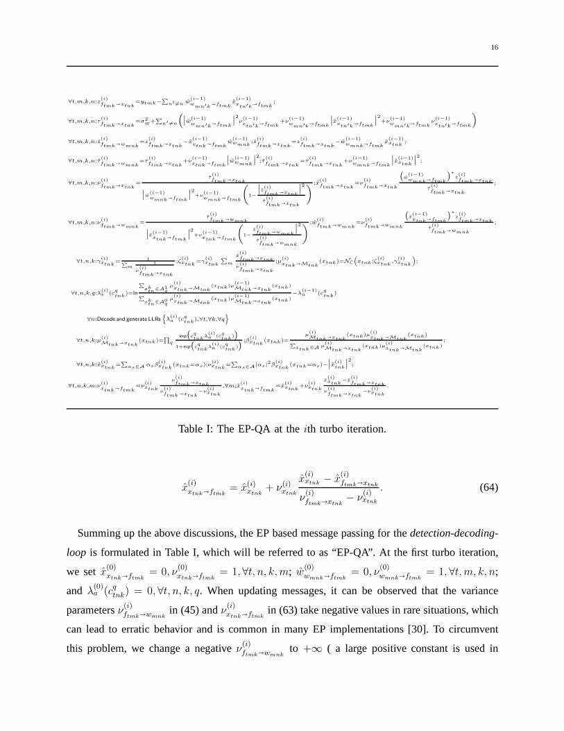
Summing up the above discussions, the EP based message passing for thedetection-decoding-
loop is formulated in Table I, which will be referred to as “EP-QA”. At the first turbo iteration,
we setx(0)xtnk�ftmk= 0, ν
(0)xtnk�ftmk
= 1, ∀t, n, k,m; w(0)wmnk�ftmk
= 0, ν(0)wmnk�ftmk
= 1, ∀t,m, k, n;
and λ(0)a (cqtnk) = 0, ∀t, n, k, q. When updating messages, it can be observed that the variance
parametersν(i)ftmk�wmnkin (45) andν(i)xtnk�ftmk
in (63) take negative values in rare situations, which
can lead to erratic behavior and is common in many EP implementations [30]. To circumvent
this problem, we change a negativeν(i)ftmk�wmnkto +∞ ( a large positive constant is used in
17
∀m,n,k:z(i)gmnk
=w(i)wmnk�gmnk
−∑
l φklh(i−1)hmnl
+ǫ(i−1)mnk
;τ(i)gmnk
=ν(i)wmnk�gmnk
+∑
l ν(i−1)hmnl
.
∀mn:τ(i)mn=
∑
k τ(i)gmnk
/K.
∀m,n,l:ξ(i)mnl
=∑
k
Φ∗kl
z(i)gmnk
τ(i)gmnk
+h(i−1)hmnl
∑
k′1
τ(i)gmnk′
−ν(i−1)hmnl
τ(i)mn
ξ(i−1)mnl
;ν(i)hmnl
= 1M
∑
m′
(
∣
∣
∣h(i−1)hm′nl
∣
∣
∣
2
+ν(i−1)hm′nl
)+∑
k1
τ(i)gmnk
;h(i)hmnl
=ν(i)hmnl
ξ(i)mnl
.
∀mn:ν(i)mn=
∑
l ν(i)hmnl
/L.
∀m,n,k:ǫ(i)mnk
=z(i)gmnk
∑
l ν(i)hmnl
+∑
l′φkl′
ν(i)hmnl′
h(i−1)hmnl′
−ν(i)mnǫ
(i−1)mnk
τ(i)gmnk
;w(i)gmnk�wmnk
=∑
l φklh(i)hmnl
−ǫ(i)mnk
;ν(i)gmnk�wmnk
=∑
l ν(i)hmnl
.
∀m,n,k:ν(i)wmnk
= 11
ν(i)gmnk�wmnk
+∑
t1
ν(i)ftmk�wmnk
,w(i)wmnk
=ν(i)wmnk
(
w(i)gmnk�wmnk
ν(i)gmnk�wmnk
+∑
t
w(i)ftmk�wmnk
ν(i)ftmk�wmnk
)
.
∀m,n,k,t:ν(i)wmnk�ftmk
= 11
ν(i)wmnk
− 1
ν(i)ftmk�wmnk
,w(i)wmnk�ftmk
=ν(i)wmnk�ftmk
(
ν(i)wmnk
w(i)wmnk
−w
(i)ftmk�wmnk
ν(i)ftmk�wmnk
)
.
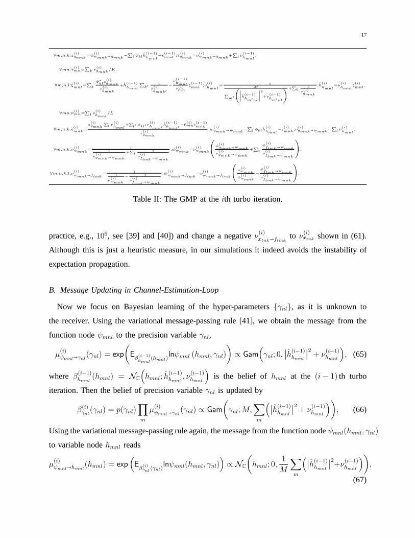
Table II: The GMP at theith turbo iteration.
practice, e.g.,106, see [39] and [40]) and change a negativeν(i)xtnk�ftmk
to ν(i)xtnk shown in (61).
Although this is just a heuristic measure, in our simulations it indeed avoids the instability of
expectation propagation.
B. Message Updating in Channel-Estimation-Loop
Now we focus on Bayesian learning of the hyper-parameters{γnl}, as it is unknown to
the receiver. Using the variational message-passing rule [41], we obtain the message from the
function nodeψmnl to the precision variableγnl,
µ(i)ψmnl�γnl
(γnl) = exp
(
Eβ(i−1)hmnl
(hmnl)lnψmnl (hmnl, γnl)
)
∝ Gam(
γnl; 0,∣∣h
(i−1)hmnl
∣∣2+ ν
(i−1)hmnl
)
, (65)
where β(i−1)hmnl
(hmnl) = NC
(
hmnl; h(i−1)hmnl
, ν(i−1)hmnl
)
is the belief of hmnl at the (i− 1) th turbo
iteration. Then the belief of precision variableγnl is updated by
β(i)γnl
(γnl) = p(γnl)∏
m
µ(i)ψmnl�γnl
(γnl) ∝ Gam
(
γnl;M,∑
m
(∣∣h
(i−1)hmnl
∣∣2+ ν
(i−1)hmnl
))
, (66)
Using the variational message-passing rule again, the message from the function nodeψmnl(hmnl, γnl)
to variable nodehmnl reads
µ(i)ψmnl�hmnl
(hmnl) = exp(
Eβ(i)γnl
(γnl)lnψmnl(hmnl, γnl)
)
∝ NC
(
hmnl; 0,1
M
∑
m
(∣∣h
(i−1)hmnl
∣∣2+ν
(i−1)hmnl
))
,
(67)
18
and the belief ofhmnl is updated byβ(i)hmnl
(hmnl) = µ(i)ψmnl�hmnl
(hmnl)∏
k µ(i)gmnk�hmnl
(hmnl),
whereµ(i)gmnk�hmnl
(hmnl) is the message fromgmnk to hmnl.
Following the derivation in [31], the Gaussian message passing for channel-estimation task, i.e.,
updating{ν(i)wmnk�ftmk, w
(i)wmnk�ftmk
}, is given by Table II, which will be referred to as “GMP”. At
the first turbo iteration, i.e.,i = 1, we set∣∣h
(0)hmnl
∣∣2+ν
(0)hmnl
= 1/L, ∀m,n, l, andξ(0)mnl = 0, ∀m,n, l.
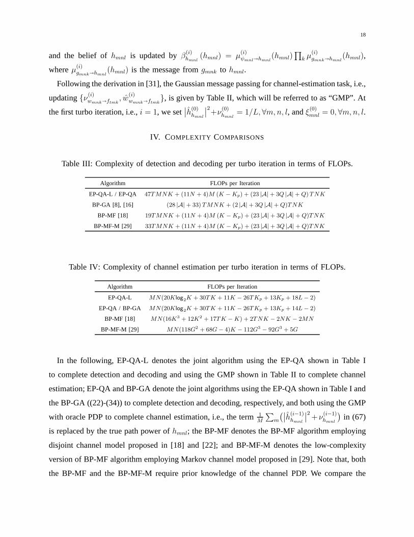
IV. COMPLEXITY COMPARISONS
Table III: Complexity of detection and decoding per turbo iteration in terms of FLOPs.
Algorithm FLOPs per Iteration
EP-QA-L / EP-QA 47TMNK + (11N + 4)M (K −Kp) + (23 |A|+ 3Q |A|+Q)TNK
BP-GA [8], [16] (28 |A|+ 33)TMNK + (2 |A|+ 3Q |A|+Q)TNK
BP-MF [18] 19TMNK + (11N + 4)M (K −Kp) + (23 |A|+ 3Q |A|+Q)TNK
BP-MF-M [29] 33TMNK + (11N + 4)M (K −Kp) + (23 |A|+ 3Q |A|+Q)TNK
Table IV: Complexity of channel estimation per turbo iteration in terms of FLOPs.
Algorithm FLOPs per Iteration
EP-QA-L MN(20Klog2K + 30TK + 11K − 26TKp + 13Kp + 18L− 2)
EP-QA / BP-GA MN(20Klog2K + 30TK + 11K − 26TKp + 13Kp + 14L− 2)
BP-MF [18] MN(16K3 + 12K2 + 17TK −K) + 2TNK − 2NK − 2MN
BP-MF-M [29] MN(118G2 + 68G − 4)K − 112G3 − 92G3 + 5G
In the following, EP-QA-L denotes the joint algorithm usingthe EP-QA shown in Table I
to complete detection and decoding and using the GMP shown inTable II to complete channel
estimation; EP-QA and BP-GA denote the joint algorithms using the EP-QA shown in Table I and
the BP-GA ((22)-(34)) to complete detection and decoding, respectively, and both using the GMP
with oracle PDP to complete channel estimation, i.e., the term 1M
∑
m
(∣∣h
(i−1)hmnl
∣∣2+ν
(i−1)hmnl
)in (67)
is replaced by the true path power ofhmnl; the BP-MF denotes the BP-MF algorithm employing
disjoint channel model proposed in [18] and [22]; and BP-MF-M denotes the low-complexity
version of BP-MF algorithm employing Markov channel model proposed in [29]. Note that, both
the BP-MF and the BP-MF-M require prior knowledge of the channel PDP. We compare the
19
Number of Subcarriers64 128 256 512 1024
Nor
mal
ized
com
plex
ity
100
101
102
103
104
105
BP-MFBP-MF-MBP-GEP-QAEP-QA-L
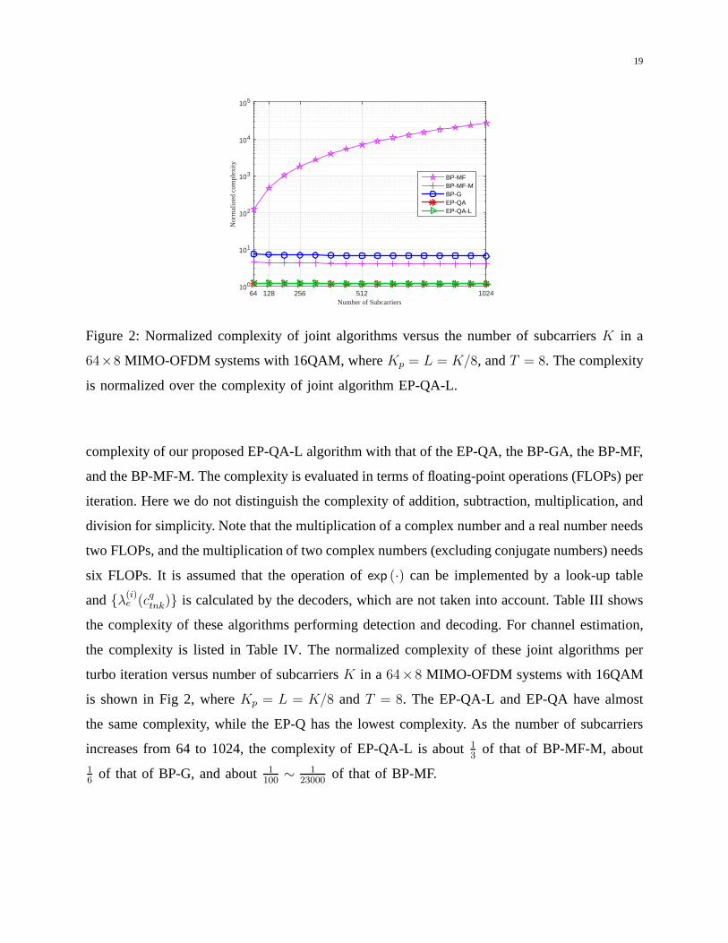
Figure 2: Normalized complexity of joint algorithms versusthe number of subcarriersK in a
64×8 MIMO-OFDM systems with 16QAM, whereKp = L = K/8, andT = 8. The complexity
is normalized over the complexity of joint algorithm EP-QA-L.
complexity of our proposed EP-QA-L algorithm with that of the EP-QA, the BP-GA, the BP-MF,
and the BP-MF-M. The complexity is evaluated in terms of floating-point operations (FLOPs) per
iteration. Here we do not distinguish the complexity of addition, subtraction, multiplication, and
division for simplicity. Note that the multiplication of a complex number and a real number needs
two FLOPs, and the multiplication of two complex numbers (excluding conjugate numbers) needs
six FLOPs. It is assumed that the operation ofexp (·) can be implemented by a look-up table
and{λ(i)e (cqtnk)} is calculated by the decoders, which are not taken into account. Table III shows
the complexity of these algorithms performing detection and decoding. For channel estimation,
the complexity is listed in Table IV. The normalized complexity of these joint algorithms per
turbo iteration versus number of subcarriersK in a 64×8 MIMO-OFDM systems with 16QAM
is shown in Fig 2, whereKp = L = K/8 andT = 8. The EP-QA-L and EP-QA have almost
the same complexity, while the EP-Q has the lowest complexity. As the number of subcarriers
increases from 64 to 1024, the complexity of EP-QA-L is about13
of that of BP-MF-M, about16
of that of BP-G, and about1100
∼ 123000
of that of BP-MF.
20
V. SIMULATION RESULTS
The proposed EP-QA-L is compared with the EP-QA, the BP-MF, the BP-MF-M, and the
BP-GA in terms of normalized mean square error (NMSE) of the channel weights and BER,
as well as the matched filter bound (MFB) that is obtained by the MAP decoding under the
condition of perfect multiuser interference cancellationand perfect channel state information
(PCSI).
Due to space constraints, a selected set of system parameters is used for simulations1. We
consider the uplink of a multiuser system withN = 8 independent users, and each user is
equipped with one transmit antenna. For each user, the transmission is based on OFDM with
K = 128 subcarriers. We choose aR = 1/2 recursive systematic convolutional (RSC) code
with generator polynomial[G1, G2] = [117, 155]oct
, followed by a random interleaver. For bit-to-
symbol mapping, multilevel Gray-mapping is used [20]. The maximum multipath delayL = 16
is assumed and the PDP is modeled as exponentially decaying,i.e., γnl = e−l/6∑L
l=1 e−l/6
, ∀n. The
CP length is set to beLcp = L and the pilot length is also set to beKp = 16. We adopt the
channel model in (1) with the spatial correlation matrix in (2). Considering a massive (16× 4)
UPA and a moderate (16 × 1) unformed linear array (ULA), we set the antenna spacing to
daz = del = λ, uniformly generate following random variables independently for each user in a
channel realization: the mean of horizontal AoDθaz in [π/6, 5π/6), the mean of vertical AoD
θel in [π/12, π/3), and the standard deviations of horizontal AoD√νaz and vertical AoD
√νel
both in [π/12, π/6). At the receiver, the BCJR algorithm is used to decode the convolutional
codes. The channels are assumed to be block-static for the selectedT = 8 transmitted OFDM
symbols.
Taking into account of the overhead incurred by the CP and thefrequency-domain pilots, the
spectral efficiencyη of the MIMO-OFDM scheme normalized by the ideal case withoutany
overhead is expressed asη = TNK−N2Kp
TN(Lcp+K)= 77.8% [35]. The energy per bit to noise power
spectral density ratioEb/N0 is defined as [42]
EbN0
=EsN0
+ 10 log10M
ηRNQ, (68)
1We will make our simulation package available for download after (possible) acceptance of the paper.
21
Eb/N0 [dB]5 5.5 6 6.5 7 7.5 8 8.5 9
NM
SE
[dB
]
-11
-10
-9
-8
-7
-6
-5
-4
-3
-2
-1
0
BP-MF-MBP-GAEP-QA-LEP-QA
Initial Turbo Iteration
Figure 3: NMSE versusEb/N0 in the 64× 8 MIMO system with 16QAM.
Eb/N0 [dB]5 5.5 6 6.5 7 7.5 8 8.5 9
NM
SE
[dB
]
-18
-16
-14
-12
-10
-8
-6
-4
-2
0
BP-MF-MBP-MFBP-GAEP-QA-LEP-QA
Initial Turbo Iteration
Figure 4: NMSE versusEb/N0 in the 16× 8 MIMO system with 16QAM.
whereEs/N is the average energy per transmitted symbol. For a fixedEb/N0, thenEs/N0 is
scaled down by the number of receive antennasM .
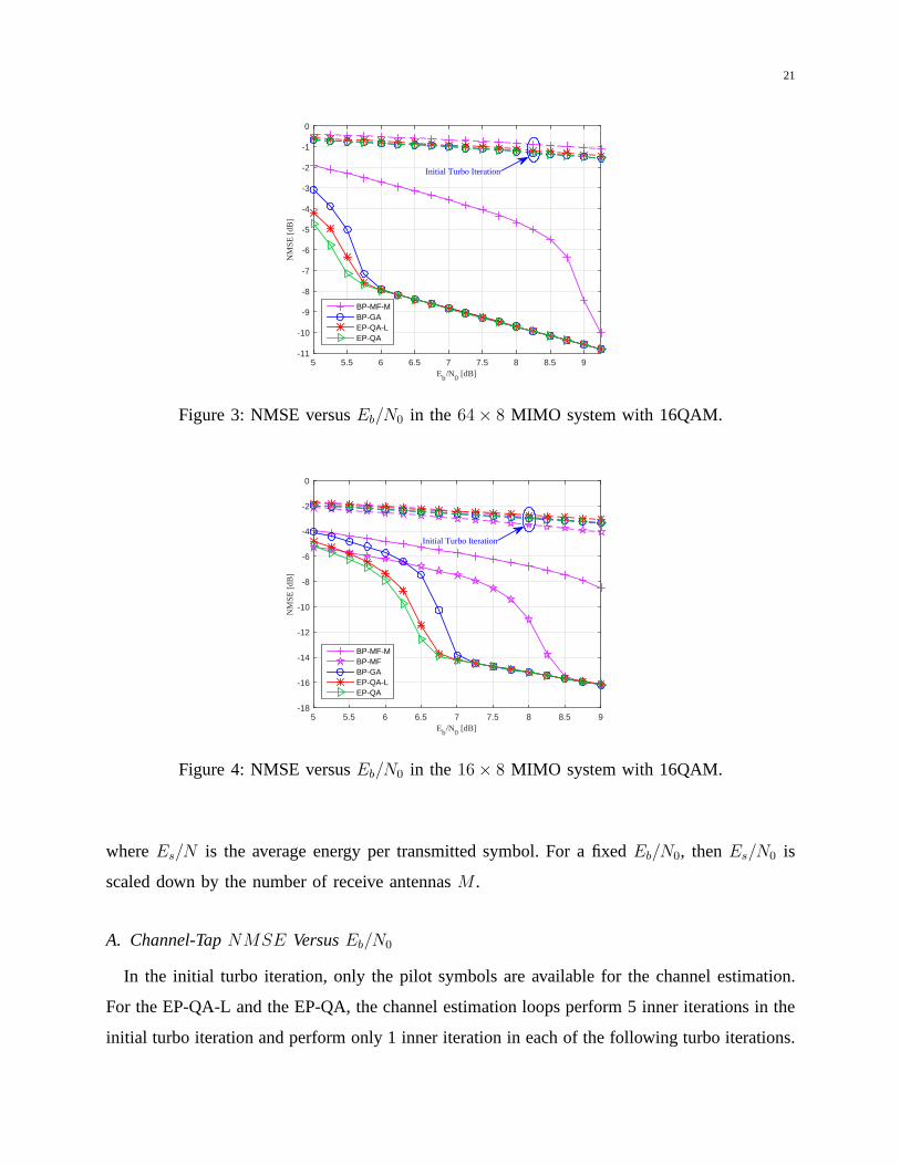
A. Channel-Tap NMSE Versus Eb/N0
In the initial turbo iteration, only the pilot symbols are available for the channel estimation.
For the EP-QA-L and the EP-QA, the channel estimation loops perform 5 inner iterations in the
initial turbo iteration and perform only 1 inner iteration in each of the following turbo iterations.
22
Eb/N0 [dB]5 5.5 6 6.5 7 7.5 8 8.5 9 9.5 10
NM
SE
[dB
]
-11
-10
-9
-8
-7
-6
-5
-4
-3
-2
-1
0
Initial-TurboBP-MF-M
(a) BP-MF-M.
Eb/N0 [dB]5 5.5 6 6.5 7 7.5 8 8.5 9
NM
SE
[dB
]
-11
-10
-9
-8
-7
-6
-5
-4
-3
-2
-1
0
Initial-TurboBP-GA
(b) BP-GA.
Eb/N0 [dB]5 5.5 6 6.5 7 7.5 8 8.5 9
NM
SE
[dB
]
-11
-10
-9
-8
-7
-6
-5
-4
-3
-2
-1
0
Initial-TurboEP-QA-L
(c) EP-QA-L.
Eb/N0 [dB]5 5.5 6 6.5 7 7.5 8 8.5 9
NM
SE
[dB
]
-11
-10
-9
-8
-7
-6
-5
-4
-3
-2
-1
0
Initial-TurboEP-QA
(d) EP-QA.
Figure 5: NMSE versusEb/N0 with multiple iterations in the64×8 MIMO system with 16QAM.
For the BP-MF, the channel estimator is equivalent to a pilot-based LMMSE estimator in the
initial turbo iteration, and becomes a data-aided LMMSE in the next turbo iterations. The channel
estimation of the BP-MF-M is performed by a Kalman smoother proposed in [29], where the
group-size of contiguous channel weights is set to beG = 4.
Fig. 3 and Fig. 4 show the NMSE of the channel estimation versus Eb/N0 in the 64 × 8
MIMO system (16 × 4 UPA) and the16 × 8 MIMO system (16 × 1 ULA), respectively. The
23
Eb/N0 [dB]8.6 8.8 9 9.2 9.4 9.6 9.8 10 10.2 10.4 10.6
NM
SE
[dB
]
-18
-16
-14
-12
-10
-8
-6
-4
-2
0
Initial-TurboBP-MF-M
(a) BP-MF-M.
Eb/N0 [dB]7 7.5 8 8.5 9 9.5
NM
SE
[dB
]
-18
-16
-14
-12
-10
-8
-6
-4
-2
0
Initial-TurboBP-MF
(b) BP-MF.
Eb/N0 [dB]5 5.5 6 6.5 7 7.5 8 8.5 9
NM
SE
[dB
]
-18
-16
-14
-12
-10
-8
-6
-4
-2
0
Initial-TurboBP-GA
(c) BP-GA.
Eb/N0 [dB]5 5.5 6 6.5 7 7.5 8 8.5 9
NM
SE
[dB
]
-18
-16
-14
-12
-10
-8
-6
-4
-2
0
Initial-TurboEP-QA-L
(d) EP-QA-L.
Eb/N0 [dB]5 5.5 6 6.5 7 7.5 8 8.5 9
NM
SE
[dB
]
-18
-16
-14
-12
-10
-8
-6
-4
-2
0
Initial-TurboEP-QA
(e) EP-QA.
Figure 6: NMSE versusEb/N0 with multiple iterations in the16×8 MIMO system with 16QAM.
24
Eb/N0 [dB]5 6 7 8 9 10 11
BE
R
10-5
10-4
10-3
10-2
10-1
BP-MF-MBP-GAEP-QA-LEP-QAMFB-PCSI
Figure 7: BER versusEb/N0 in the 64× 8 MIMO system with 16QAM.
NMSE at theith turbo iteration is calculated by
NMSE =1
Θ
Θ∑
θ=1
1
MN
M∑
m=1
N∑
n=1
∑Ll=1
∣∣hmnl − h
(i)mnl
∣∣2
∑L
l=1 |hmnl|2
, (69)
whereΘ is the number of Monte Carlo runs. It is shown that the NMSE of the proposed EP-QA-
L outperforms other algorithms including the BP-GA, the BP-MF-M, and the BP-MF (which
is evaluated only in the16 × 8 MIMO system due to complexity issue). It is also shown that,
compared with the EP-QA using oracle channel PDP, the EP-QA-L is slightly degraded only in
the low region ofEb/N0. The NMSE of BP-MF-M is higher than that of all other algorithms
at the point that the number of turbo iterations is 15.
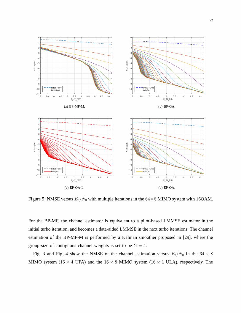
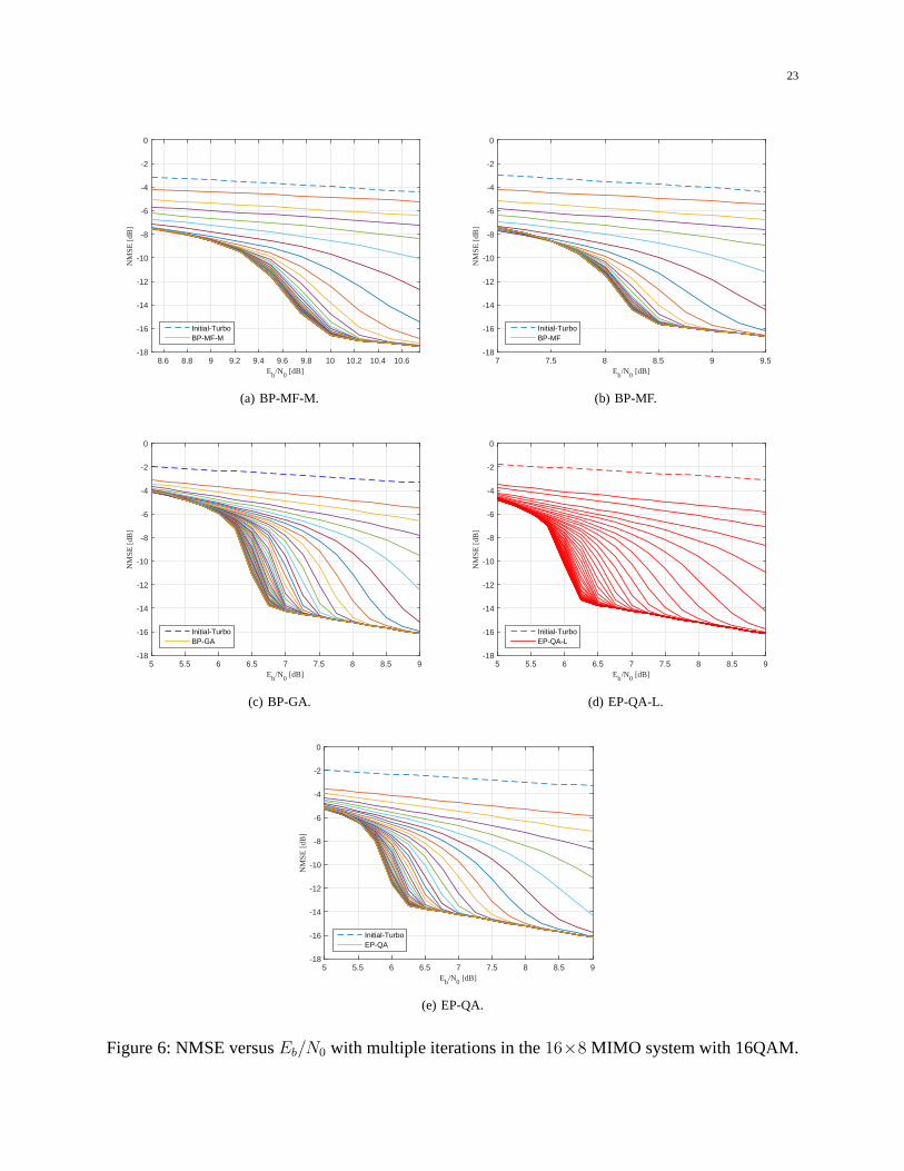
Fig. 5 and Fig. 6 present the NMSE performance with increasing number of turbo iterations.
In the high region ofEb/N0, it can be seen that 10 turbo iterations are enough for all the
algorithms to achieve convergence. In the lowEb/N0 region, the EP-QA-L (and the EP-QA
with oracle PDP) can uniformly improve the NMSE performanceby increasing the number of
turbo iterations, but other algorithms can’t.
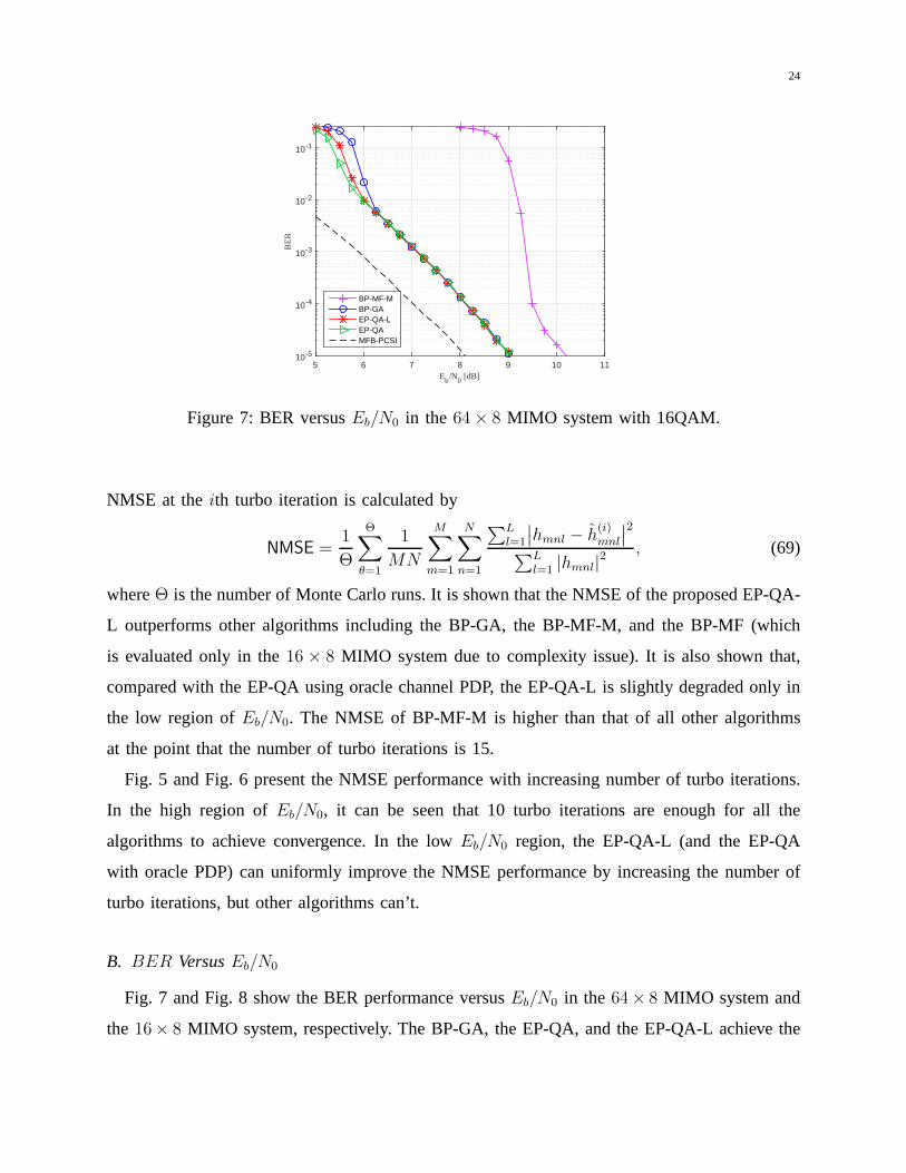
B. BER Versus Eb/N0
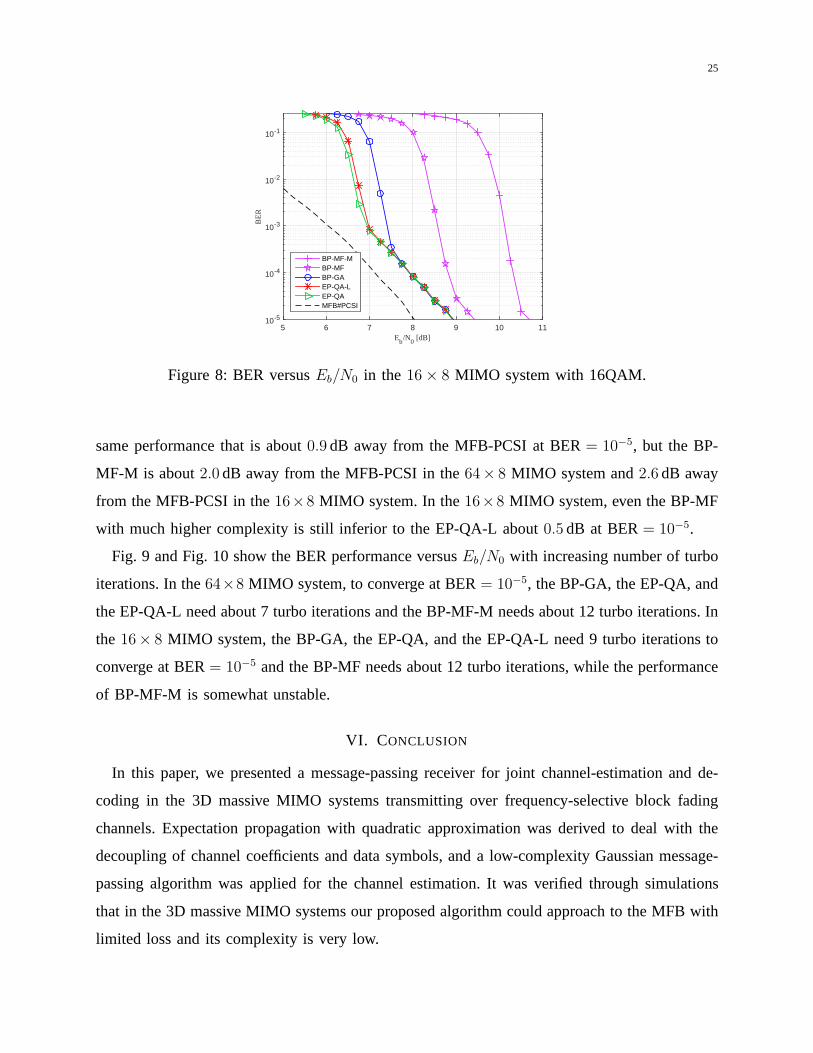
Fig. 7 and Fig. 8 show the BER performance versusEb/N0 in the 64× 8 MIMO system and
the 16× 8 MIMO system, respectively. The BP-GA, the EP-QA, and the EP-QA-L achieve the
25
Eb/N0 [dB]5 6 7 8 9 10 11
BE
R
10-5
10-4
10-3
10-2
10-1
BP-MF-MBP-MFBP-GAEP-QA-LEP-QAMFB#PCSI
Figure 8: BER versusEb/N0 in the 16× 8 MIMO system with 16QAM.
same performance that is about0.9 dB away from the MFB-PCSI at BER= 10−5, but the BP-
MF-M is about2.0 dB away from the MFB-PCSI in the64× 8 MIMO system and2.6 dB away
from the MFB-PCSI in the16×8 MIMO system. In the16×8 MIMO system, even the BP-MF
with much higher complexity is still inferior to the EP-QA-Labout0.5 dB at BER= 10−5.
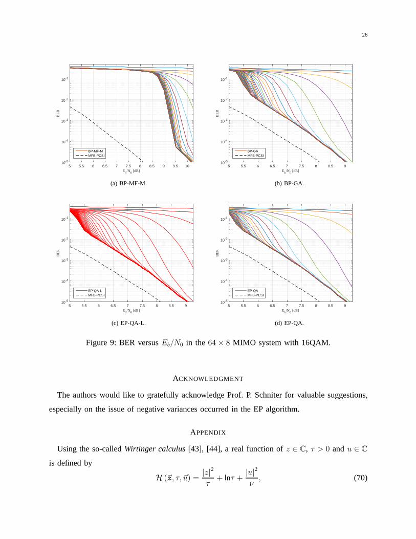
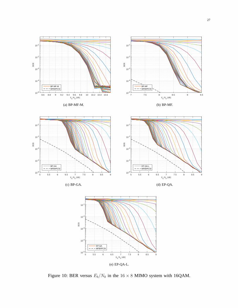
Fig. 9 and Fig. 10 show the BER performance versusEb/N0 with increasing number of turbo
iterations. In the64×8 MIMO system, to converge at BER= 10−5, the BP-GA, the EP-QA, and
the EP-QA-L need about 7 turbo iterations and the BP-MF-M needs about 12 turbo iterations. In
the 16× 8 MIMO system, the BP-GA, the EP-QA, and the EP-QA-L need 9 turbo iterations to
converge at BER= 10−5 and the BP-MF needs about 12 turbo iterations, while the performance
of BP-MF-M is somewhat unstable.
VI. CONCLUSION
In this paper, we presented a message-passing receiver for joint channel-estimation and de-
coding in the 3D massive MIMO systems transmitting over frequency-selective block fading
channels. Expectation propagation with quadratic approximation was derived to deal with the
decoupling of channel coefficients and data symbols, and a low-complexity Gaussian message-
passing algorithm was applied for the channel estimation. It was verified through simulations
that in the 3D massive MIMO systems our proposed algorithm could approach to the MFB with
limited loss and its complexity is very low.
26
Eb/N0 [dB]5 5.5 6 6.5 7 7.5 8 8.5 9 9.5 10
BE
R
10-5
10-4
10-3
10-2
10-1
BP-MF-MMFB-PCSI
(a) BP-MF-M.
Eb/N0 [dB]5 5.5 6 6.5 7 7.5 8 8.5 9
BE
R
10-5
10-4
10-3
10-2
10-1
BP-GAMFB-PCSI
(b) BP-GA.
Eb/N0 [dB]5 5.5 6 6.5 7 7.5 8 8.5 9
BE
R
10-5
10-4
10-3
10-2
10-1
EP-QA-LMFB-PCSI
(c) EP-QA-L.
Eb/N0 [dB]5 5.5 6 6.5 7 7.5 8 8.5 9
BE
R
10-5
10-4
10-3
10-2
10-1
EP-QAMFB-PCSI
(d) EP-QA.
Figure 9: BER versusEb/N0 in the 64× 8 MIMO system with 16QAM.
ACKNOWLEDGMENT
The authors would like to gratefully acknowledge Prof. P. Schniter for valuable suggestions,
especially on the issue of negative variances occurred in the EP algorithm.
APPENDIX
Using the so-calledWirtinger calculus [43], [44], a real function ofz ∈ C, τ > 0 andu ∈ C
is defined by
H (~z, τ, ~u) =|z|2τ
+ lnτ +|u|2ν, (70)
27
Eb/N0 [dB]8.6 8.8 9 9.2 9.4 9.6 9.8 10 10.2 10.4 10.6
BE
R
10-5
10-4
10-3
10-2
10-1
BP-MF-MMFB#PCSI
(a) BP-MF-M.
Eb/N0 [dB]7 7.5 8 8.5 9 9.5
BE
R
10-5
10-4
10-3
10-2
10-1
BP-MFMFB#PCSI
(b) BP-MF.
Eb/N0 [dB]5 5.5 6 6.5 7 7.5 8 8.5 9
BE
R
10-5
10-4
10-3
10-2
10-1
BP-GAMFB#PCSI
(c) BP-GA.
Eb/N0 [dB]5 5.5 6 6.5 7 7.5 8 8.5 9
BE
R
10-5
10-4
10-3
10-2
10-1
EP-QA-LMFB#PCSI
(d) EP-QA.
Eb/N0 [dB]5 5.5 6 6.5 7 7.5 8 8.5 9
BE
R
10-5
10-4
10-3
10-2
10-1
EP-QAMFB#PCSI
(e) EP-QA-L.
Figure 10: BER versusEb/N0 in the 16× 8 MIMO system with 16QAM.
28
where the conjugate coordinates~z and ~u are defined by~z , [z, z∗]T and ~u , [u, u∗]T
respectively, andν > 0 is a constant. For the functionH (~z, τ, ~u), some of its partial derivations
are given by
∂H∂~z
,
[∂H∂z
,∂H∂z∗
]
=
[z∗
τ,z
τ
]
, (71)
∂2H∂~z∂~z
,
∂∂z
(∂H∂z
)∗ ∂∂z∗
(∂H∂z
)∗
∂∂z
(∂H∂z∗
)∗ ∂∂z∗
(∂H∂z∗
)∗
=
1τ
0
0 1τ
, (72)
∂H∂τ
=1
τ− |z|2
τ 2, (73)
∂H∂~u
,
[∂H∂u
,∂H∂u∗
]
=[u∗ν,u
ν
]
, (74)
∂2H∂~u∂~u
,
∂∂u
(∂H∂u
)∗ ∂∂u∗
(∂H∂u
)∗
∂∂u
(∂H∂u∗
)∗ ∂∂u∗
(∂H∂u∗
)∗
=
1ν
0
0 1ν
. (75)
Up to the second order, the power series expansion ofH (~z, τ, ~u) at the point(~z0, τ0, ~u0) is
given by [44]
H (~z, τ, ~u) ≈ H (~z0, τ0, ~u0) +∂H∂~z0
∆~z +∂H∂τ0
∆τ +∂H∂~u0
∆~u
+1
2(∆~z)H
∂2H∂~z0∂~z0
∆~z +1
2(∆~u)H
∂2H∂~u0∂~u0
∆~u
= H (~z0, τ0, ~u0) + 2ℜ{z∗0τ0∆z +
u∗0
ν
∆u
}
− |z0|2τ 20
∆τ +1
τ0∆τ +
1
τ0|∆z|2 + 1
ν|∆u|2 , (76)
where∆~z , ~z − ~z0, ∆τ , τ − τ0 and∆~u , ~u− ~u0
REFERENCES
[1] T. L. Marzetta, “Noncooperative cellular wireless withunlimited numbers of base station antennas,”IEEE Trans. Wireless
Commun., vol. 9, no. 11, pp. 3590–3600, Nov. 2010.
[2] F. Rusek, D. Persson, B. K. Lau, E. G. Larsson, T. L. Marzetta, O. Edfors, and F. Tufvesson, “Scaling up MIMO:
Opportunities and challenges with very large arrays,”IEEE Signal Process. Mag., vol. 30, no. 1, pp. 40–60, Jan. 2013.
[3] J. Hoydis, S. ten Brink, and M. Debbah, “Massive MIMO in the UL/DL of cellular networks: How many antennas do we
need?”IEEE J. Sel. Areas Commun., vol. 31, no. 2, pp. 160–171, Feb. 2013.
[4] E. G. Larsson, O. Edfors, F. Tufvesson, and T. L. Marzetta, “Massive MIMO for next generation wireless systems,”IEEE
Communications Magazine, vol. 52, no. 2, pp. 186–195, February 2014.
29
[5] N. Shariati, E. Björnson, M. Bengtsson, and M. Debbah, “Low-complexity polynomial channel estimation in large-scale
MIMO with arbitrary statistics,”IEEE J. Sel. Topics in Signal Process., vol. 8, no. 5, pp. 815–830, Oct. 2014.
[6] S. Noh, M. D. Zoltowski, Y. Sung, and D. J. Love, “Pilot beam pattern design for channel estimation in massive MIMO
systems,”IEEE J. Sel. Topics in Signal Process., vol. 8, no. 5, pp. 787–801, Oct. 2014.
[7] P. S. Rossi and R. R. Müller, “Joint twofold-iterative channel estimation and multiuser detection for MIMO-OFDM
systems,”IEEE Trans. Wireless Commun., vol. 7, no. 11, pp. 4719–4729, Nov. 2008.
[8] C. Novak, G. Matz, and F. Hlawatsch, “IDMA for the multiuser MIMO-OFDM uplink: A factor graph framework for joint
data detection and channel estimation,”IEEE Trans. Signal Process., vol. 61, no. 16, pp. 4051–4066, Aug. 2013.
[9] Y. Liu, Z. Tan, H. Hu, L. J. Cimini, and G. Y. Li, “Channel estimation for OFDM,” IEEE Communications Surveys &
Tutorials, vol. 16, no. 4, pp. 1891–1908, Fourth Quarter 2014.
[10] P. Zhang, S. Chen, and L. Hanzo, “Embedded iterative semi-blind channel estimation for three-stage-concatenatedMIMO-
aided QAM turbo transceivers,”IEEE Trans. Veh. Technol., vol. 63, no. 1, pp. 439–446, Jan. 2014.
[11] J. Ma and P. Li, “Data-aided channel estimation in largeantenna systems,”IEEE Trans. Signal Process., vol. 62, no. 12,
pp. 3111–3124, June 2014.
[12] S. Park, B. Shim, and J. W. Choi, “Iterative channel estimation using virtual pilot signals for MIMO-OFDM systems,”
IEEE Trans. Signal Process., vol. 63, no. 12, pp. 3032–3045, June 2015.
[13] F. R. Kschischang, B. J. Frey, and H.-A. Loeliger, “Factor graphs and the sum-product algorithm,”IEEE Trans. Inf. Theory,
vol. 47, no. 2, pp. 498–519, Feb. 2001.
[14] A. P. Worthen and W. E. Stark, “Unified design of iterative receivers using factor graphs,”IEEE Trans. Inf. Theory, vol. 47,
no. 2, pp. 843–849, 2001.
[15] H. Wymeersch,Iterative Receiver Design. Cambridge, U.K.: Cambridge Univ. Press, 2007.
[16] Y. Liu, L. Brunel, and J. J. Boutros, “Joint channel estimation and decoding using Gaussian approximation in a factor
graph over multipath channel,” inProc. Int. Symp. on Personal, Indoor and Mobile Radio Commun. (PIMRC), 2009, pp.
3164–3168.
[17] G. E. Kirkelund, C. N. Manchón, L. P. B. Christensen, E. Riegler, and B. H. Fleury, “Variational message-passing forjoint
channel estimation and decoding in MIMO-OFDM,” inProc. IEEE Global Telecomm. Conf. (GLOBECOM ), 2010, pp.
1–6.
[18] C. N. Manchón, G. E. Kirkelund, E. Riegler, L. P. B. Christensen, and B. H. Fleury, “Receiver architectures for MIMO-
OFDM based on a combined VMP-SP algorithm,”arXiv: 1111.5848, 2011.
[19] Q. Guo and D. D. Huang, “EM-based joint channel estimation and detection for frequency selective channels using gaussian
message passing,”IEEE Trans. Signal Process., vol. 59, no. 8, pp. 4030–4035, 2011.
[20] P. Schniter, “A message-passing receiver for BICM-OFDM over unknown clustered-sparse channels,”IEEE J. Sel. Topics
in Signal Process., vol. 5, no. 8, pp. 1462–1474, 2011.
[21] C. Knievel, P. A. Hoeher, A. Tyrrell, and G. Auer, “Multi-dimensional graph-based soft iterative receiver for MIMO-
OFDM,” IEEE Trans. Commun., vol. 60, no. 6, pp. 1599–1609, June 2012.
[22] E. Riegler, G. E. Kirkelund, C. N. Manchón, M.-A. Badiu,and B. H. Fleury, “Merging belief propagation and the mean
field approximation: A free energy approach,”IEEE Trans. Inf. Theory, vol. 59, no. 1, pp. 588–602, Jan. 2013.
[23] X. Zhang, P. Xiao, D. Ma, and J. Wei, “Variational-bayes-assisted joint signal detection, noise covariance estimation, and
channel tracking in MIMO-OFDM systems,”IEEE Trans. Veh. Technol., vol. 63, no. 9, pp. 4436–4449, Nov. 2014.
30
[24] D. D. Lin and T. J. Lim, “A variational inference framework for soft-in soft-out detection in multiple-access channels,”
IEEE Trans. Inf. Theory, vol. 55, no. 5, pp. 2345–2364, May 2009.
[25] P. Schniter, “Joint estimation and decoding for sparsechannels via relaxed belief propagation,” inProc. of 44th Asilomar
Conference on Signals, Systems and Computers. (ASILOMAR). IEEE, 2010, pp. 1055–1059.
[26] M.-A. Badiu, G. E. Kirkelund, C. N. Manchón, E. Riegler,and B. H. Fleury, “Message-passing algorithms for channel
estimation and decoding using approximate inference,” inProc. IEEE Int. Symp. Inf. Theory (ISIT), 2012, pp. 2376–2380.
[27] A. Drémeau, C. Herzet, and L. Daudet, “Boltzmann machine and mean-field approximation for structured sparse
decompositions,”IEEE Trans. Signal Process., vol. 60, no. 7, pp. 3425–3438, July 2012.
[28] F. Krzakala, A. Manoel, E. Tramel, and L. Zdeborová, “Variational free energies for compressed sensing,” inProc. IEEE
International Symposium on Information Theory (ISIT), June 2014, pp. 1499–1503.
[29] M.-A. Badiu, C. Manchón, and B. Fleury, “Message-passing receiver architecture with reduced-complexity channel
estimation,”IEEE Commun. Lett., vol. 17, no. 7, pp. 1404–1407, Jul. 2013.
[30] T. P. Minka, “A family of algorithms for approximate Bayesian inference,” Ph.D. dissertation, Massachusetts Institute of
Technology, 2001.
[31] S. Wu, L. Kuang, Z. Ni, J. Lu, D. D. Huang, and Q. Guo, “Expectation propagation approach to joint channel estimation
and decoding for OFDM systems,” inProc. IEEE Int. Conf. on Acoust., Speech and Signal Process. (ICASSP), Florence,
Italy, May 2014, pp. 1941–1945.
[32] J. T. Parker, P. Schniter, and V. Cevher, “Bilinear generalized approximate message passing–Part I: Derivation,”IEEE
Trans. Signal Process., vol. 62, no. 22, pp. 5839–5853, Nov. 2014.
[33] L. Schumacher, K. Pedersen, and P. Mogensen, “From antenna spacings to theoretical capacities-guidelines for simulating
MIMO systems,” inProc. IEEE Int. Symp. PIMRC, 2002, pp. 587–592.
[34] D. Ying, F. W. Vook, T. A. Thomas, D. J. Love, and A. Ghosh,“Kronecker product correlation model and limited feedback
codebook design in a 3D channel model,” inProc. of 2014 IEEE International Conference on Communications (ICC),
Jun. 2014, pp. 5865–5870.
[35] L. Dai, Z. Wang, and Z. Yang, “Spectrally efficient time-frequency training OFDM for mobile large-scale MIMO systems,”
IEEE J. Sel. Areas Commun., vol. 3, no. 2, pp. 251–263, Feb. 2013.
[36] P. Som, T. Datta, N. Srinidhi, A. Chockalingam, and B. Rajan, “Low-complexity detection in large-dimension MIMO-ISI
channels using graphical models,”IEEE J. Sel. Topics in Signal Process., vol. 5, no. 8, pp. 1497–1511, Dec. 2011.
[37] C. M. Bishopet al., Pattern recognition and machine learning. New York: Springer, 2006.
[38] J. Hu, H.-A. Loeliger, J. Dauwels, and F. Kschischang, “A general computation rule for lossy summaries/messages with
examples from equalization,” inProc. 44th Allerton Conf. Communication, Control, and Computing, 2006, pp. 27–29.
[39] M. R. Andersen, A. Vehtari, O. Winther, and L. K. Hansen,“Bayesian inference for spatio-temporal spike and slab priors,”
arXiv:1509.04752, 2015.
[40] D. Hernández-Lobato, J. M. Hernández-Lobato, and P. Dupont, “Generalized spike-and-slab priors for Bayesian group
feature selection using expectation propagation,”The Journal of Machine Learning Research, vol. 14, no. 1, pp. 1891–
1945, 2013.
[41] J. M. Winn and C. M. Bishop, “Variational message passing,” The Journal of Machine Learning Research, vol. 6, pp.
661–694, 2005.
[42] B. M. Hochwald and S. ten Brink, “Achieving near-capacity on a multiple-antenna channel,”IEEE Trans. Commun., vol. 51,
no. 3, pp. 389–399, Mar. 2003.

31
[43] A. Van Den Bos, “Complex gradient and Hessian,” inIEE Proc. Vis., Image and Signal Processing, vol. 141, no. 6. IET,
1994, pp. 380–383.
[44] K. Kreutz-Delgado, “The complex gradient operator andthe CR-calculus,”arXiv preprint arXiv:0906.4835, 2009.


![Sparse Doubly-Selective Channel Estimation Techniques for … · 2020. 5. 27. · passing (AMP) approach has been developed in [15] with its application to sparse channel estimation](https://img.pdfslide.us/doc/110x75/61176e0b18692452b6640d95/sparse-doubly-selective-channel-estimation-techniques-for-2020-5-27-passing.jpg)