MEASURING TRENDS IN LEISURE: THE ALLOCATION …faculty.chicagobooth.edu/erik.hurst/research/aguiar_hurst_leisure... · MEASURING TRENDS IN LEISURE: THE ALLOCATION OF TIME OVER FIVE

1

MEASURING TRENDS IN LEISURE: THE ALLOCATION OF TIME OVER FIVE DECADES*

Mark Aguiar and Erik Hurst

In this paper, we use five decades of time-use surveys to document trends in the

allocation of time within the United States. We find that a dramatic increase in leisure

time lies behind the relatively stable number of market hours worked between 1965 and

2003. Specifically, using a variety of definitions for leisure, we show that leisure for men

increased by roughly 6‒9 hours per week (driven by a decline in market work hours) and

for women by roughly 4‒8 hours per week (driven by a decline in home production work

hours). Lastly, we document a growing inequality in leisure that is the mirror image of the

growing inequality of wages and expenditures, making welfare calculation based solely

on the latter series incomplete.

* We would like to thank Lawrence Katz and four anonymous referees for detailed, helpful comments. We also thank Susanto Basu, Gary Becker, Kathy Bradbury, Kerwin Charles, Raj Chetty, Steve Davis, Jordi Galí, Reuben Gronau, Dan Hamermesh, Chad Jones, Ellen McGrattan, Bruce Meyer, Kevin Murphy, Derek Neal, Valerie Ramey, Richard Rogerson, Frank Stafford, Jay Stewart, Justin Wolfers, and seminar participants at the Minneapolis Federal Reserve, the Cleveland Federal Reserve (NBER EFG/RSW meeting), the University of Rochester, the University of Wisconsin’s Institute for Poverty Research Summer Institute, NBER Summer Institute in Labor Studies, the University of California at San Diego, the University of California at Berkeley, the University of Chicago, Columbia University, Boston College, Harvard, Wharton, and the University of Maryland. We thank Dan Reichgott for research assistance. Hurst would like to acknowledge the financial support of the University of Chicago’s Graduate School of Business. This paper was written while Aguiar was employed at the Federal Reserve Bank of Boston. The views expressed in this paper are solely those of the authors and do not reflect official positions of the Federal Reserve Bank of Boston or the Federal Reserve System.

2

I. INTRODUCTION

In this paper, we document trends in the allocation of time within the United

States over the last 40 years. In particular, we focus our attention on the evolution of

leisure time. In commonly used household surveys designed to measure labor market

activity (such as the Current Population Survey (CPS) and the Panel Study of Income

Dynamics (PSID)), the only category of time use that is consistently measured is market

work hours.1 As a result, leisure is almost universally defined as time spent away from

market work. However, as noted by Becker [1965], households can also allocate time to

production outside the formal market sector. To the extent that non-market (home)

production is important and changing over time, changes in leisure time will be poorly

proxied by changes in time spent away from market work. By linking five decades of

detailed time-use surveys, we empirically draw the distinction between leisure and the

complement of market work. In doing so, we document a set of facts about how home

production and leisure have evolved for men and women of differing educational

attainment during the last 40 years.

The main empirical finding in this paper is that leisure time—measured in a

variety of ways—has increased significantly in the United States between 1965 and 2003.

When computing our measures of leisure, we separate out other uses of household time,

including time spent in market work, time spent in non-market production, time spent

obtaining human capital, and time spent in heath care. Given that some categories of time

use are easier to categorize as leisure than others, we create four distinct measures of

leisure. Our measures range from the narrow, which includes activities designed to yield

3

direct utility, such as entertainment, socializing, active recreation, and general relaxation,

to the broad, namely, time spent neither in market production nor in non-market

production. While the magnitudes differ slightly, the conclusions drawn are similar

across each of the leisure measures.

Using a narrow definition of leisure (our Leisure Measure 2), we find that leisure

increased by 6.2 hours per week for men and by 4.9 hours per week for women between

1965 and 2003, adjusting for changing demographics. Interestingly, the decline in total

work (the sum of total market work and total non-market work) was nearly identical for

both men and women (8.3 and 7.8 hours per week, respectively). These declines in total

work are large. To put things in perspective, in 1965 the average man spent 61 hours per

week and the average women spent 55 hours per week in combined market and non-

market work. The 8-plus hour-per-week decline recorded between 1965 and 2003

therefore represents roughly 14 percent of the total work week in 1965.

The adjustments that allow for greater leisure while satisfying the time budget

constraint differ between men and women. Men increased their leisure by allocating less

time to the market sector, whereas leisure time for women increased simultaneously with

time spent in market labor. The increased leisure for women was made possible by a

more than 10 hour-per-week decline in the time allocated to home production. This

decline more than offset their 3.8 hour-per-week increase in time spent in market work

during this time period.2

We analyze trends in child care separately from trends in other types of home

production. There is an increase of roughly 2 hours per week in reported time spent on

child care in the 2003 survey relative to earlier surveys. In light of the conceptual difficulty

4

in classifying whether time spent with children represents work or leisure, we treat child

care as a separate category and then explore the robustness of our conclusions to a variety

of different assumptions about how child care should be classified. The alternative

classification of child care as work or leisure does not influence the overall trends

through 1993, as the reported time spent in child care was essentially flat between 1965

and 1993. Moreover, the 2 hour-per-week increase in child care between 1993 and 2003

is modest relative to the large changes in total work and leisure recorded between 1965

and 2003.

We also document a growing cross-sectional dispersion in time allocated to

leisure. The gap between the 90th and 10th percentiles of the cross-sectional leisure

distribution increased by 14 hours per week between 1965 and 2003. Other measures tell

a similar story of a growing dispersion in the consumption of leisure time. Some of this

increase in dispersion we can link to the fact that less educated men and women

experienced much greater increases in leisure compared to their more educated

counterparts. For example, between 1965 and 2003, men with a high school diploma

experienced an increase of 7.3 hours per week in our second narrowest leisure category,

while men with at least a bachelor’s degree experienced no change. The relative growth

of leisure favoring less educated adults is consistent with the finding that low wage workers

have dramatically decreased their market work hours relative to high wage workers over

the last century (see Costa [2000]).

This divergence in leisure we document started during the last half of our sample.

The increase in leisure between 1965 and 1985 was similar for respondents of different

educational attainment. Post 1985, on the other hand, less educated adults experienced

5

significantly larger gains in leisure compared to those with a college education or more.

The timing of the changing inequality in leisure across education groups mirrors the well

documented timing of the changing inequality in wages and consumption (see Katz and

Autor [1999] and Attanasio et al. [2004] for wages and consumption, respectively).

We also document a significant dispersion of leisure within educational

categories. Using the decomposition of Juhn, Murphy and Pierce [1993], we show that

the majority of the increase in the overall cross-sectional dispersion in leisure was due to

forces other than observed demographics (including education). That is, while the

growing leisure gap between educational groups is substantial, it is more than matched by

the growing within-group dispersion.

Our work adds to the existing literature on measuring changes in the allocation of

time. Three classic book-length references are Ghez and Becker [1975], Juster and

Stafford [1985], and Robinson and Godbey [1999]. The latter is most closely related to

our study. It uses the same time-use surveys we use from 1965, 1975, and 1985, as well

as some additional time-use information from the early 1990s.3 However, aside from

examining trends over longer periods of time, our paper extends the literature by

documenting and analyzing the growing dispersion in leisure. Moreover, we consider

alternative leisure aggregates. Lastly, instead of reporting unconditional means, we

report trends in time use adjusted for changing demographics. This is potentially

important given the changes in the age distribution, fertility, family structure and

educational attainment which occurred during this time period. While the literature, on

the allocation of time is large, particularly in sociology, to the best of our knowledge, no

other study combines the length of time series, the attention to cross-sectional dispersion

6

(particularly post-1985), and the focus on different measures of leisure found in the

current paper.

II. EMPIRICAL TRENDS IN THE ALLOCATION OF TIME

II.A. Data

To document the trends in the allocation of time over the last 40 years, we link

five major time use surveys: 1965-1966 America’s Use of Time; 1975-1976 Time Use in

Economics and Social Accounts; 1985 Americans’ Use of Time; 1992-1994 National

Human Activity Pattern Survey; and the 2003 American Time Use Survey.4 The Data

Appendix and Table I describe these surveys in detail. All data and programs used to

create the results in this paper are available on the authors’ websites. In this section, we

characterize four major uses of time: market work, non-market production, child care,

and leisure.

Our primary sample consists of respondents aged 21 through 65 who are neither

students nor retirees.5 We drop adults younger than 21 and adults older than 65 (as well

as students and early retirees) to minimize the role of time allocation decisions that have

a strong inter-temporal component, such as education and retirement. Moreover, the 1965

time-use survey excludes households with heads who are either retired or over the age of

65. We drop these households from subsequent surveys to ensure a consistent sample.

Additionally, the 1965, 1975, and 1985 time-use surveys exclude individuals under the

age of 18 or 19 from their samples.6

We report trends over the last 40 years holding constant the demographic

composition of the sample. Specifically, we divide the sample into demographic cells

defined by 5 age groups (21-29, 30-39, 40-49, 50-59, 60-65), 4 education categories (less

7

than high school, high school, some college, and college degree or more), 2 sex

categories, and whether or not there is a child present in the household. We do not create

separate cells distinguishing child status for respondents aged 60-65 due to the small

number that have children present in the home. This division yields 72 demographic

cells. Note that due to the limited demographics in the 1993 survey, we cannot create

consistent cells for the full sample based on marital status, the number of children in the

household, or the age of the children. However, we discuss below the robustness of our

results when we exclude the 1993 survey and create cells in the remaining years that also

differentiate respondents by marital status, the number of children, and the age of the

children. Previewing these results, conditioning on these additional controls has a

minimal effect on the trends documented in Tables II and III.

To calculate the constant weights used for our demographic adjustments, we pool

together all of our time use data sets and compute the percentage of the population that

resides in each demographic cell. These weights are denoted by the 72×1 vector W.7

Following Katz and Murphy [1992], we use these fixed weights to calculate weighted

means for each activity in each year. Specifically, if Yjt is the 72×1 vector of cell means

for activity j in year t, we calculate the demographically-adjusted average time spent in

activity j in year t as W′Yjt. Means for subsamples based on sex and education are

calculated in a similar manner with the weights scaled to sum to one. Unless otherwise

stated, all magnitudes reported in the paper are for constant demographic weights.8

However, in Section II.G below, we address how much of the unconditional trends in

time use can be explained by changing demographics.

8

The demographic adjustment is necessary given the significant demographic

changes in the United States over the last 40 years. Since 1965, the average American

has aged, become more educated, become more likely to be single, and had fewer

children. All of these changes may affect how an individual chooses to allocate his or her

time. By fixing the demographic weights, we are reporting how time spent in a given

activity has changed during the last 40 years adjusted for these demographic changes.

II.B. Trends in Market Work

Trends in market work over the last half century have been well documented (see,

for example, McGrattan and Rogerson [2004]). The major difference between our results

and those using traditional household surveys such as the CPS and PSID is that our

research focuses on changes in the allocation of household time across market work, non-

market work, and leisure, while the existing research tends to focus exclusively on

changes in market hours. As we show in this paper, the conclusions about changing

leisure drawn solely from time spent working in the market sector are misleading.

We define market work in two ways. “Core” market work includes all time spent

working in the market sector on main jobs, second jobs, and overtime, including any time

spent working at home.9 This market work measure is analogous to the market work

measures in the Census, the PSID, or the Survey of Consumer Finances (SCF). The

broader category “total” market work is core market work plus time spent commuting

to/from work and time spent on ancillary work activities (for example, time spent at work

on breaks or eating a meal).

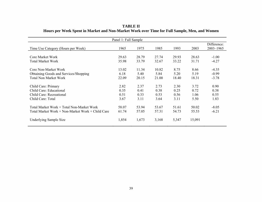
The time trend in core market work and total market work for all individuals, men

and women are shown in Panels 1, 2, and 3 of Table II, respectively. Average hours per

9

week of core market work for non-retired, working-age adults were essentially constant

between 1965 and 2003 (Panel 1). However, as is well known, this relatively stable

average masks the fact that market work hours for men have fallen and market work

hours for women have increased. Specifically, core market work hours for males fell by

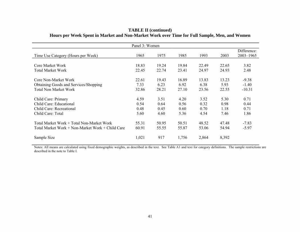
6.6 hours per week between 1965 and 2003 (Panel 2) and increased by 3.8 hours per

week for women (Panel 3). The increase in core market work hours for women occurred

continuously between 1965 and 1993, before stabilizing in the last decade. These trends

in male and female labor force participation and work hours have been well documented

in the literature.10

The decline in market work for men is relatively larger using our broader measure

of “total market work.” Specifically, total market work declined by 12.1 hours per week,

as opposed to 6.6 hours per week for core market work. The difference stems primarily

from a decline in breaks at work, perhaps reflecting the decline over this period in

unionized manufacturing jobs in which breaks are clearly delineated. For women, the

increase in total market work was slightly smaller than the increase in core market work

(2.5 vs. 3.8 hours per week).

II.C. Trends in Non-Market Work

Unlike the trends in time spent in market work, the trends in time spent in “non-

market” work between 1965 and 2003 have been relatively unexplored.11 We define

three categories of time spent on non-market production. Throughout the remainder of

the paper, time spent on an activity includes any time spent on transportation associated

with that activity.

10

First, we define time spent on “core” non-market work. This includes any time

spent on meal preparation and cleanup, doing laundry, ironing, dusting, vacuuming,

indoor household cleaning, and indoor design and maintenance (including painting and

decorating). Second, we analyze time spent “obtaining goods and services.” This

category includes time spent acquiring any good or service (excluding medical care,

education, and restaurant meals). Examples include grocery shopping, shopping for other

household items, comparison shopping, coupon clipping, going to the bank, going to a

barber, going to the post office, and buying goods on-line. The last category we analyze

is “total non-market work” which includes time spent in core non-market work and time

spent obtaining goods and services plus time spent on other home production such as

home maintenance, outdoor cleaning, vehicle repair, gardening, and pet care. This latter

category is designed to be a complete measure of non-market work excluding child care.

Below, we separately discuss and analyze trends in child care.

As reported in Table II Panel 1, while core market work hours for the full sample

have been relatively constant over the last 40 years, time spent in non-market work has

fallen sharply. Specifically, time spent in core non-market work has fallen by 4.4 hours

per week, time spent obtaining goods and services has fallen by 1.0 hour per week, and

total non-market work has fallen by 3.8 hours per week. As with market work hours, the

average trends mask differences across sexes. Male total non-market work hours have

actually increased by 3.8 hours per week while female total non-market work hours have

fallen by 10.3 hours per week.

Disaggregating the changes in time spent on non-market work into its three

components, we find that for women, time spent on core non-market work decreased by

11

9.4 hours per week and time spent obtaining goods and services decreased by 1.4 hours

per week. Women slightly increased time spent on other non-market work by 0.5 hours

per week. For men, time spent on core non-market work increased by 1.4 hours per week

and time spent on other non-market work increased by 2.8 hours per week. Men,

however, experienced a decline in time spent obtaining goods and services of 0.5 hours

per week.

II.D. Trends in Child Care

Child care poses both conceptual as well as measurement challenges. It has been

argued that child care differs from housework in terms of the utility generated. For

example, when asked to assess the satisfaction they receive from the various activities

they perform, individuals consistently rank time spent playing with their children and

reading to their children as being among the most enjoyable (Robinson and Godbey

[1999]). Additionally, individuals consistently report that general child care is more

enjoyable than activities such as housework, grocery shopping, yard work, cleaning the

house, doing dishes, and doing laundry.12 Such survey evidence suggests that it may be

appropriate to examine trends in child care separately from trends in other categories of

non-market production.

Also, from the standpoint of empirical implementation, there is some ambiguity

about whether childcare is treated consistently across all surveys. Robinson and Godbey

[1999] raise several concerns about the comparability of 1993 childcare measures to the

measures of childcare in the other surveys. Egerton et al. [2006] also caution against

making comparisons between the 1993 and 2003 time use surveys. In the absence of a

12

firm consensus on this point, we adopt a conservative approach that analyzes child care

separately from other components of non-market production.

We define primary child care as any time spent on the basic needs of children,

including breast feeding, rocking a child to sleep, general feeding, changing diapers,

providing medical care (either directly or indirectly), and grooming. Note that time spent

preparing a child’s meal is included in general meal preparation, a component of non-

market production. We define educational child care as any time spent developing

children’s cognitive skills including reading to children, teaching children, helping

children with homework, and attending meetings at a child’s school. We define

recreational child care as playing games with children, playing outdoors with children,

attending a child’s sporting event or dance recital, going to the zoo with children, and

taking walks with children. Total child care is defined as the sum of these three measures.

In Table II, we show the evolution of hours per week spent in all four of these

child care measures. Despite a slight decline in time allocated to child care between 1965

and 1993, there was a 2.4-hours-per-week increase in reported time spent on total child

care across all individuals between 1993 and 2003. Note that this number pools together

households with and without children. Conditional on having a child, the increase in

child care between 1993 and 2003 was over five hours per week.

The pattern occurred for both sexes. For all women (men), total child care

increased by nearly 3 (1.8) hours per week between 1993 and 2003 after remaining

roughly constant between 1965 and 1993. Additionally, this recent increase in time spent

in total child care is reflected in all sub-components. Specifically, women increased their

time spent on primary child care by 1.8 hours per week, on educational child care by 0.7

13

hours per week, and on recreational child care by 0.5 hours per week. Lastly, after being

relatively flat between 1965 and 1993, similar increases in time spent in child care

occurred across all demographic groups between 1993 and 2003 (results not shown). The

demographic groups included highly-educated and less-educated men and women,

married and single men and women with children, and working and non-employed men

and women. For example, women with children and a high school education or less

experienced an increase in the time spent in total childcare of 6.4 hours per week between

1993 and 2003. The increase for women with children who had at least some college

education was also 6.4 hours per week.

While the increase in child care between 1993 and 2003 may have resulted from

an actual change in household behavior, it may also be the result of differences in the

measurement across the surveys. Given the potential measurement problem with child

care across surveys, along with the conceptual problem of whether the marginal hour of

time spent with children is work or leisure, we have chosen to examine child care as a

separate category.13 In doing so, we discuss the robustness of our main results to the

inclusion of child care as a component of total work and then, separately, to the inclusion

of child care as a component of leisure. However, it is important to note that time spent

in child care was essentially flat between 1965 and 1993. As a result, it does not matter

how child care is classified for trends between 1965 and 1993. Additionally, given that

child care increased similarly for all broad demographic groups between 1993 and 2003,

the treatment of child care has essentially no effect on the conclusions about the changing

dispersion of leisure discussed in Section III.

14

II.E. Trends in Total Work

We combine total market work with total non-market work to compute a measure

of “total work.” To start, our measure of total work excludes time spent in child care.

Table II documents the changes in total work between 1965 and 2003. For the full

sample, total work has fallen by 8.1 hours per week. A striking result is that the decline in

total market work is nearly identical for men and women. Between 1965 and 2003, men

and women decreased their total work hours by 8.3 and 7.8 hours per week, respectively.

The similarity is surprising, given the increase in the relative wage of women over this

period and the simultaneous increase in the market work hours of women. This places a

strong restriction on theories explaining the increase in female labor force participation.

If one adds total child care to our benchmark total work measure, the full sample

records a decline of 6.2 hours per week. Men and women experienced declines of 6.5

and 6.0 hours per week, respectively. As discussed above, all of the difference in the

trends due to the inclusion of child care occurred between 1993 and 2003.

The results in Table II provide a dramatically different picture for the evolution of

time allocation than one usually infers from standard household surveys that measure

only time spent in market work. Specifically, the dramatic increase in the market work

hours of women masks a decline in total work hours. Women have experienced a decline

of over 10 hours per week in the time they spend on home production—an amount that is

nearly three times as large as their increase in time spent in market work. In other words,

for women, changes in market work reveal little about changes in total work.

Another important consideration raised by the trends in total work hours is

whether the economy is on a balanced growth path. Taken as a whole, the strong

downward trend in total work (market plus non-market work) suggests that the economy

15

may not be on a balanced growth path, although this does not rule out the possibility that

the economy may asymptote to such a path. The relatively stable figure for market work

hours per adult over the last 40 years (in the presence of steady increases in real incomes)

is often used to justify utility functions in which the income and substitution effects of

wage changes cancel.14 If non-market work yields a disutility similar to that of market

work, the downward trend in the sum of these variables suggests that this assumption

may be inappropriate.

II.F. Trends in Leisure

In this sub-section, we proceed by exploring four alternative definitions of leisure.

The reason we explore different measures of leisure is that the classification of leisure

activities can be somewhat subjective. As we show, our various measures tell a fairly

consistent story regarding the past 40 years, making much of the ambiguity of what

actually constitutes leisure empirically unimportant.

The means of our four leisure measures are reported in Table III. Our narrowest

measure of leisure, Leisure Measure 1, sums together all time spent on

“entertainment/social activities/relaxing” and “active recreation” described in appendix

Table A1. These categories include any activity that are pursued solely for direct

enjoyment such as television watching, leisure reading, going to parties, relaxing, going

to bars, playing sports, surfing the web, and visiting friends. We include gardening and

time spent with pets in our leisure measures. This is the only set of activities that is

classified as both leisure and home production.15 Pet care provides direct utility but is

also something one can purchase on the market. Conceptually, gardening is more likely

to be considered a hobby, while cutting grass and raking leaves is more likely to be seen

as work (of course, this is subject to debate). However, the data do not let us draw the

16

distinction between gardening and yard work consistently throughout the sample. In the

pre-2003 surveys, yard work is included in outdoor home maintenance, while gardening

is a separate activity. Unfortunately, in 2003, yard work is not differentiated from

gardening. However, as can be seen in Figure I (described below), this activity is a small

component of total leisure and plays little role in generating the overall trends.

As seen in Table III, Leisure Measure 1 increased by 4.6 hours per week for the

full sample, by 5.6 hours per week for men, and 3.7 hours per week for women. Leisure 1

increased fairly consistently for men between 1965 and 2003. However, for women,

Leisure 1 increased monotonically between 1965 and 1993 and then declined between

1993 and 2003. The entire decline between 1993 and 2003 can be explained by the

increase in child care in this interval. However, regardless of such measurement issues,

our basic measure of leisure increased dramatically for both men and women between

1965 and 2003.16

Biddle and Hamermesh [1990] argue that certain time activities may enhance

production in the market and non-market sectors. For example, they provide a model in

which time spent sleeping is a choice variable that both augments productivity and enters

the utility function directly. Furthermore, they provide strong empirical evidence

showing that sleep time is, in fact, a choice variable over which individuals optimize. For

example, individuals sleep more on the weekends and on vacations. Similar conceptual

points apply broadly to time spent eating and on personal care. In this spirit, we define

Leisure Measure 2 as activities that provide direct utility but may also be viewed as

intermediate inputs. Specifically, Leisure Measure 2 includes Leisure Measure 1 as well

as time spent in sleeping, eating, and personal care. While we exclude own medical care,

17

we include such activities as grooming, having sex, sleeping or napping, and eating at

home or in restaurants.

Leisure Measure 2 increased by 5.5 hours per week between 1965 and 2003. In

other words, in addition to the increase in Leisure Measure 1, time spent in sleeping,

eating, and personal care increased by an additional 1 hour per week between 1965 and

2003. Over this period, Leisure Measure 2 increased by 6.2 hours per week for men and

by 4.9 hours per week for women.

Our third leisure category, Leisure Measure 3, includes Leisure Measure 2 plus

time spent in child care. The inclusion of child care has very little effect on trends

between 1965 and 1993, but it does make a difference regarding the change over the last

decade. Leisure 3 increased by 7.3 hours per week for the full sample, by 8.0 hours per

week for men and 6.8 hours per week for women.

As noted above, Leisure Measure 4 is the residual of total work. The difference

between Leisure Measures 3 and 4 includes time spent in education, civic and religious

activities (going to church, volunteering, social clubs, etc.), caring for other adults, and

own medical care. Between 1965 and 2003, civic activities fell by 30 minutes per week,

education (omitting students) fell by 18 minutes per week, own medical care increased by

38 minutes per week, and care for other adults increased by one hour per week (with all

of the latter increase taking place between 1993 and 2003).

In Figure I, we explore the trends in the individual components of Leisure 2 for

the full sample. The line labeled “Leisure 2” reflects the corresponding row in Panel 1 of

Table III. More than 100 percent of the increase in leisure can be accounted for by the

increase in the time spent watching television, which totals 7.4 hours per week for the full

18

sample, 6.7 hours per week for men, and 8.0 hours per week for women. This increase in

television is offset by a 3.9 hour-per-week decline in socializing (going to parties, bars,

etc.) and a 3.1 hour-per-week decline in reading (books, magazines, letters, etc.). The

sharp decline in socializing reinforces the evidence of Putnam [2000], which documents a

decline in social interactions using a variety of data sources. Small changes were

recorded for categories such as gardening/pet-care, hobbies, and other entertainment

(plays, movies, radio, records, computers, etc.).

In short, leisure has increased by between 4.6 hours per week (Leisure Measure 1)

and 8.1 hours per week (Leisure Measure 4) for the average non-retired adult since 1965.

These magnitudes are economically large. In 1965, the average individual spent 30 hours

per week in core market work (roughly 4 hours per day). The gain in total leisure

between 1965 and 2003 is therefore equal to an increase of between 15 percent (Leisure

Measure 1) and 27 percent (Leisure Measure 4) of the average core market work week in

1965. Or, if one assumes a 40-hour work week, the increase in leisure is equivalent to 5.9

to 10.5 additional weeks of vacation per year.

The trends documented above are computed for fixed demographic composition,

defined by age, sex, education, and the presence of children in the household. We can

refine our demographic categories by omitting the 1993 survey, which has the least

demographic detail. We have explored the robustness of our conclusions to conditioning

on marital status, the number of children, and the age of the youngest child, in addition to

age, education, and sex. The results for men were similar to those reported in Tables II

and III. The additional demographic controls play a somewhat larger role for women.

For example, the additional controls reduced the increase in Leisure 2 for women (men)

19

by roughly one hour (23 minutes) per week. The details are reported in the robustness

appendix posted on the authors’ websites.

There are two reasons to believe that the increase in leisure that we have

documented may be biased downwards. First, we are measuring changes in leisure only

for non-retired individuals. The fact that individuals are living longer and are retiring

earlier, coupled with the fact that retired individuals enjoy more leisure than non-retired

households (Hamermesh [2006]), imply that the increase in lifetime leisure is much larger

than we document.

Second, there has been a claim that the nature of time spent at work has changed

over the last decade. While at work, individuals may engage in more leisure-type

activities like corresponding through personal email or surfing the web. The time diaries

do not separate out the type of tasks individuals perform while at work, so it is hard to

test this claim formally within our data. If this shift in the nature of time spent at work

has occurred, it accentuates the increase in leisure we document.

II.G. The Role of Demographics in Mean Trends

Throughout, we have presented changes in time use between 1965 and 2003

conditional on demographics. We have yet to discuss how much of the unconditional

change in time use can be explained by changing demographics. To explore this, we

conduct a Blinder-Oaxaca style decomposition of the unconditional mean change in time

use into the portion that can be explained by changing demographics and the portion than

can be explained by changes within demographic groups.

20

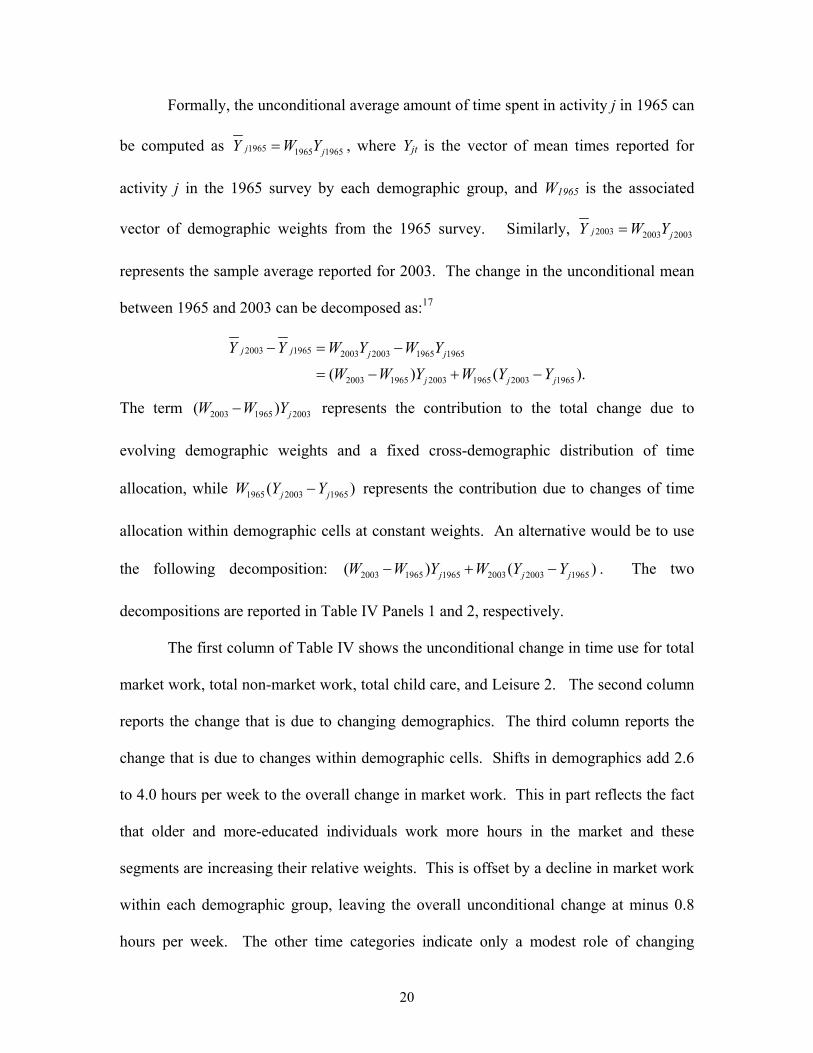
Formally, the unconditional average amount of time spent in activity j in 1965 can

be computed as 1965 1965 1965j jY W Y= , where Yjt is the vector of mean times reported for

activity j in the 1965 survey by each demographic group, and W1965 is the associated

vector of demographic weights from the 1965 survey. Similarly, 2003 2003 2003j jY W Y=

represents the sample average reported for 2003. The change in the unconditional mean

between 1965 and 2003 can be decomposed as:17

2003 1965 2003 2003 1965 1965

2003 1965 2003 1965 2003 1965( ) ( ).j j j j

j j j

Y Y W Y W Y

W W Y W Y Y

− = −

= − + −

The term 2003 1965 2003( ) jW W Y− represents the contribution to the total change due to

evolving demographic weights and a fixed cross-demographic distribution of time

allocation, while 1965 2003 1965( )j jW Y Y− represents the contribution due to changes of time

allocation within demographic cells at constant weights. An alternative would be to use

the following decomposition: 2003 1965 1965 2003 2003 1965( ) ( )j j jW W Y W Y Y− + − . The two

decompositions are reported in Table IV Panels 1 and 2, respectively.

The first column of Table IV shows the unconditional change in time use for total

market work, total non-market work, total child care, and Leisure 2. The second column

reports the change that is due to changing demographics. The third column reports the

change that is due to changes within demographic cells. Shifts in demographics add 2.6

to 4.0 hours per week to the overall change in market work. This in part reflects the fact

that older and more-educated individuals work more hours in the market and these

segments are increasing their relative weights. This is offset by a decline in market work

within each demographic group, leaving the overall unconditional change at minus 0.8

hours per week. The other time categories indicate only a modest role of changing

21

demographics in explaining the overall trends in unconditional means. Much of the trend

is due to within demographic cell changes rather than evolving demographics. This result

will be echoed in the analysis of leisure dispersion in the next section. Note as well that

the change in Leisure 2 due to changing demographic weights is larger in Panel 1. This

reflects that leisure differences between demographic groups are larger in 2003 than in

1965, a point also developed in the next section.

III. LEISURE INEQUALITY

The previous section documented a mean decline in total work for both men and

women over the last 40 years. In this section, we consider how other moments of the

leisure distribution evolved with the aim of documenting the evolution of leisure

inequality. We show that the inequality in leisure increased both between and within

educational categories.

The evolution of several key percentiles of the Leisure 2 distribution is depicted

in Figure II. Specifically, for each year, we calculate the 10th, 25th, 50th, 75th, and 90th

percentiles of Leisure 2, unconditional on demographics.18 The figure depicts a general

fanning out of the leisure distribution over the last 40 years. Notice further that all of the

percentile points of the leisure distribution, except the 10th, recorded increases between

1965 and 2003. In other words, besides fanning out, the leisure distribution also shifted

upwards.

Figure III plots the hour-per-week change in Leisure 2 for each percentile

between 1965 and 2003. That is, for each percentile point, we subtract the hours per

week of leisure in 1965 for a given percentile point from that percentile point’s hours per

week of leisure in 2003. The fact that Leisure 2 is bounded below by zero and above by

22

the constraint of 24 hours in a day implies that changes in the extreme percentiles tend

toward zero. As a result, the figure only depicts percentiles 5 through 95. Note that the

percentiles refer to the sample distributions and the differences are not adjusted for

demographics. The figure shows that the change in leisure time essentially increased

linearly with the percentile of the leisure distribution. That is, the patterns depicted in

Figure II are replicated throughout the entire leisure distribution.

To gain additional insight into the increasing dispersion, we examine the extent to

which leisure has become more unequal between education groups. Table V reports the

demographically-adjusted time spent in market work, total non-market work, and Leisure

2 for men and women, broken down by educational attainment during 1965, 1985, and

2003. Our education categories are less than a high school diploma (<12), a high school

diploma or GED equivalent (12), some college (13-15), and a college degree or more

(16+). In 1965, men spent roughly 50 hours per week in market work, with little

variation across educational categories. Moreover, in 1965, the time spent in leisure was

similar as well. For example, men with less than a high school degree spent 104 hours

per week in Leisure Measure 2 while college-educated men spent 102 hours per week.

For women, the college educated spent more hours in market work in 1965 (27

hours per week) relative to high school graduates (23 hours per week) and high school

dropouts (18 hours week). This pattern was reversed for non-market work, with college

educated women performing 7 hours less non-market work per week than high school

dropouts. In terms of leisure, college educated women enjoyed the same leisure as high

school graduates and 4 hours less leisure per week than high school dropouts, a pattern

similar to that for men.

23

However, the rough equality in leisure time observed in 1965 disappeared over

the subsequent four decades. Specifically, men with a college degree experienced no

change in Leisure 2 between 1965 and 2003. Male high school dropouts, on the other

hand, experienced an increase of 12.2 hours per week and male high school graduates

experienced an increase of 7.3 hours per week. The corresponding increase for female

college graduates is 1.3 hours per week versus 7.9 hours per week for high school

dropouts and 6.3 hours per week for high school graduates.

Table V indicates that this divergence in leisure time for both men and women is

due primarily to differences in market work. Less-educated and highly educated males

increased total non-market work hours by similar amounts between 1965 and 2003.

Conversely, total market work hours fell by a much greater amount between 1965 and

2003 for less-educated males (-18.0 for less than high school, -13.7 for high school, and -

4.4 for college graduates). The net result is that leisure increased relatively more for less-

educated men than was the case for their more highly educated counterparts due to a shift

out of market work.

For women, high school dropouts experienced a decline of 10.1 hours per week in

total non-market work versus 8.5 hours for college educated women. However, during

this time period, total market work hours increased much more for highly educated

females than for less-educated females. Specifically, college graduates increased their

total market work hours by 4.3 hours per week, while high school graduates increased

market work by 2.0 hours per week and those with less than a high school degree

decreased market work by 2.4 hours per week.

We should note that the divergence in leisure times across education groups

24

occurred primarily post 1985. Table VI illustrates this point by showing the difference in

the change in Leisure 2 between individuals with a college education or more and the

other three educational groups over the first half and then the latter half of our sample.

Table VI pools together men and women. Between 1965 and 1985, respondents with less

than a high school degree, a high school degree, and some college, experienced gains in

leisure relative to college educated individuals of 0.5, 1.6, and 0.4 hours per week,

respectively. These differences indicate that leisure gains were shared fairly evenly

across education groups in the first half of our sample. However, between 1985 and

2003, the relative gains in leisure over college educated individuals were 8.9, 4.6 and 3.4

hours per week, respectively, for individuals with less than a high school degree, a high

school degree, or some college. This growing gap in leisure mirrors the well documented

change in wages and consumption between education groups starting in the early 1980s

(see Katz and Autor [1999] and Attanasio et al. [2004] for wages and consumption,

respectively). Specifically, the 1980s and 1990s were decades in which higher educated

individuals experienced increases in wages and consumption relative to their less

educated counterparts.19 If leisure time has value, our results suggest that welfare

calculations about the growing inequality based solely on changing incomes or changing

expenditures may be incomplete.

One concern with the results regarding educational status is that the marginal high

school graduate in 1965 differs from that in 2003. In particular, 73 percent of our sample

in 1965 had a high school education or less, while the corresponding figure for 2003 is 42

percent. However, the percentiles presented in Figure II indicate that the growing

inequality occurs throughout the distribution. Moreover, as a robustness exercise we

25

have also split the sample in two at approximately the 70th percentile by education in

1965, 1985, and 2003. The dividing line corresponds to a high school degree in 1965 and

some college in 1985 and 2003. We found that within the bottom 70 percentiles of the

education distribution, leisure increased by 7.7 and 5.8 hours per week for men and

women, respectively. The corresponding increases in leisure for individuals within the

top 30 percentiles were 1.0 and 1.2 hours per week, respectively.20 Again, most of the

divergence was in the latter half of the sample. This confirms that the separation between

educational categories is not simply a result of the changing composition of high school

graduates.

In Table VII we explore whether there are differences between educational groups

in terms of which leisure activities experienced the largest changes. Specifically, Table

VII reports the 1965-2003 change in the major sub-components of Leisure 2 broken

down by educational attainment. The table indicates that all education groups increased

television watching substantially. Those with less than a high school degree increased

their television watching by 9.3 hours per week. The corresponding number for high

school graduates was 7.8 hours per week. Perhaps surprisingly, given the small overall

increase in Leisure 2, college graduates increased their television watching by 5.5 hours

per week. This increase in time spent watching television for highly educated individuals

was offset by a decline in the time spent socializing and reading of 5.4 and 3.5 hours per

week, respectively. The net result was only a 0.6 hour per week increase in Leisure 2 for

college graduates between 1965 and 2003. The other educational categories also

experienced significant declines in the time spent reading and socializing, although these

declines were smaller than those for college graduates and smaller than the corresponding

26

categories’ increase in time spent watching television. The most educated respondents

also recorded declines of 1.4 hours per week in sleeping and personal care, compared to

an increase of 3.2 hours per week for this category among high school dropouts.

Conversely, highly educated individuals increased the time they spent eating while less-

educated individuals experienced a decline in time spent on this activity.

Aside from a growing inequality between educational groups, Figure IV shows

that there has also been a growing inequality within educational groups. Figure IV

replicates Figure III but breaks the sample down by educational attainment. Specifically,

we compare the change in leisure by percentile for the sample of respondents within each

of our four educational groups. The figure indicates that the positive correlation between

changes in leisure time and the initial level of leisure time occurs within each educational

category. The figure also indicates that the pattern is more pronounced for those with

less education.

To further explore what is driving the growing dispersion in leisure, we perform a

decomposition using the methodology of Juhn, Murhpy, and Pierce [1993], henceforth

JMP, which examined the changing wage distribution. In particular, let Yit denote the

amount of time allocated to Leisure 2 in survey year t for respondent i. The cross-

sectional variation can be jointly explained by demographics, X, and a residual term, uit:

(1) it it t itY X uβ= + .

Our X controls include dummy variables for the corresponding interactions between age,

sex, education, and fertility. In particular, we include 72 dummy variables that

correspond to the 72 demographic cells discussed in Section II used to compute our

demographically adjusted weights.21 The elements of βt therefore represent demographic

cell means.22 We run this regression separately using data from each year of our sample.

27

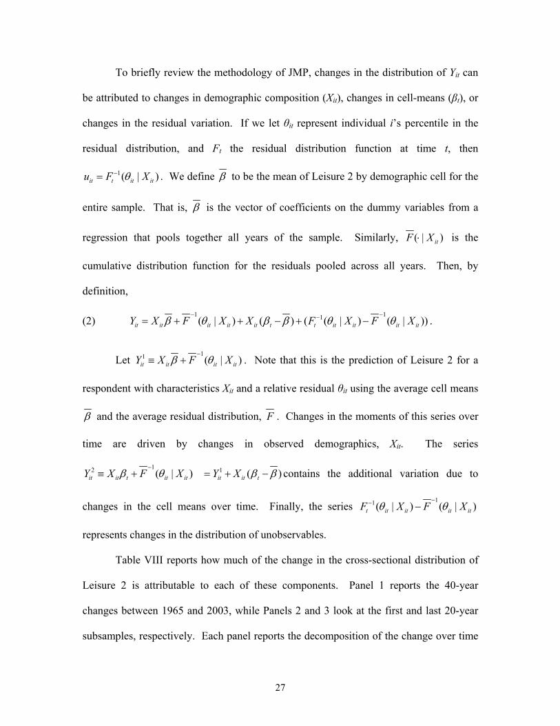
To briefly review the methodology of JMP, changes in the distribution of Yit can

be attributed to changes in demographic composition (Xit), changes in cell-means (βt), or

changes in the residual variation. If we let θit represent individual i’s percentile in the

residual distribution, and Ft the residual distribution function at time t, then

1( | )it t it itu F Xθ−= . We define β to be the mean of Leisure 2 by demographic cell for the

entire sample. That is, β is the vector of coefficients on the dummy variables from a

regression that pools together all years of the sample. Similarly, ( | )itF X⋅ is the

cumulative distribution function for the residuals pooled across all years. Then, by

definition,

(2) 1 11( | ) ( ) ( ( | ) ( | ))it it it it it t t it it it itY X F X X F X F Xβ θ β β θ θ− −−= + + − + − .

Let

11 ( | )it it it itY X F Xβ θ−

≡ + . Note that this is the prediction of Leisure 2 for a

respondent with characteristics Xit and a relative residual θit using the average cell means

β and the average residual distribution, F . Changes in the moments of this series over

time are driven by changes in observed demographics, Xit. The series

12 ( | )it it t it itY X F Xβ θ−

≡ + 1 ( )it it tY X β β= + − contains the additional variation due to

changes in the cell means over time. Finally, the series 11( | ) ( | )t it it it itF X F Xθ θ−− −

represents changes in the distribution of unobservables.

Table VIII reports how much of the change in the cross-sectional distribution of

Leisure 2 is attributable to each of these components. Panel 1 reports the 40-year

changes between 1965 and 2003, while Panels 2 and 3 look at the first and last 20-year

subsamples, respectively. Each panel reports the decomposition of the change over time

28

in the difference between the 90th and 10th percentiles, the 90th and 50th percentiles, and

the 50th and 10th percentiles. The first column reports the total change. Taking the first

row, the 90-10 differential increased by 14.2 hours per week between 1965 and 2003.

Demographics, as captured by 1itY defined above, predict a change of -0.8 hours per week,

as reported in the 2nd column. The fact that changes to demographic quantities explains

little of the change in leisure inequality is reminiscent of the Blinder-Oaxaca

decompositions of changes in means presented in Table IV. The third column reports the

change in the 90-10 differential for 2itY once we subtract the second column’s change in

1itY . This term represents the additional contribution to dispersion due to changes in cell

means and totals 2.7 hours per week. The remainder, 12.3 hours per week, is attributed

to unobservables and represents the bulk of the total change. A similar pattern is repeated

for the other measures of cross-sectional dispersion. The one sub-period for which the

change in between-group means plays a substantial role is the period 1985—2003. As

discussed above this is the sub-period during which educational differences in leisure

became prominent. For this period, roughly 40 percent of the increased dispersion

represented in each of the three measures can be attributed to changing demographic-

group means.

IV. DISCUSSION AND CONCLUSION

In this paper, we have documented that the amount of leisure enjoyed by the

average American has increased substantially over the last 40 years. This increase is

observable across a number of sub-samples. In particular, women have increased their

market labor force participation while at the same time enjoying more leisure. Moreover,

29

the increase in leisure time occurred during a period in which average market work hours

were relatively constant.

Our results also document a dramatic increase in the dispersion of leisure. Much

of this dispersion occurred within demographic groups, but some can be attributed to

differences across educational groups. In particular, we find that less-educated adults

have increased their relative consumption of leisure, particularly in the last 20 years.

This corresponds to a period in which wages and consumption expenditures increased

faster for highly educated adults. This divergence suggests a different relationship

between income and leisure in the cross-section compared to the time-series. In the first

part of the paper, we documented a large increase in leisure over the last 40 years,

potentially suggesting that higher income implies greater leisure. However, the recent

divergence in leisure between educational groups suggests that, cross-sectionally, lower

incomes imply more leisure. These trends are coupled with the fact that the early time

use surveys (particularly the ones from 1965 and 1985) suggest that leisure is invariant to

education in the cross section. The larger increase in leisure for less-educated adults is an

empirical implication that any quantitative model should match.

Our evidence on leisure dispersion has a parallel in the longer run trends in

market labor supply. Costa [2000] documents that low-wage workers reduced their

market work hours relative to high-wage workers between the 1890s and 1991. In

particular, at the turn of the 20th century, low-wage workers worked longer hours than

high-wage workers. This differential disappeared by the early 1970s, and during the last

30 years high-wage workers supplied relatively more market hours. Similarly, we find

small differences in leisure across educational categories in 1965, and a sharp relative

30

increase in leisure favoring less educated adults over the subsequent 40 years.

We acknowledge that any definition that distinguishes “leisure” from “work” is a

matter of judgment. Some work activities may generate direct utility, whether at a formal

job or while cooking and shopping. Similarly, such leisure activities as reading a book or

watching TV may add to one’s human capital or be directly job related and therefore be

considered market substitutes. Our response to this ambiguity has been to present a wide

range of evidence. The decline in home production and the time-series and cross-

sectional patterns in leisure are generally robust to these variations. Regardless of one’s

preferred definition of leisure, the fact remains that large changes have occurred in the

allocation of time over the last 40 years. Many of these changes concern activities away

from the market, making conclusions drawn solely from observations on market work

hours potentially misleading.

The present study focuses exclusively on the United States. There are studies that

compare the United States and Europe at a point in time (for example, see Freeman and

Schettkat [2005] and Ragan [2006]). However, to our knowledge, there are no other

research papers using data from other countries that perform a time-series analysis similar

to the one above. One country that has conducted a consistent time use survey during the

last forty years is Norway. According to published Norwegian statistics, between 1971

and 2000, Norwegian men and women increased their “leisure” by roughly 7 and 8 hours

per week, respectively.23 These findings are similar to the results we documented for the

United States. How changes in the time spent in leisure experienced in the United States

compares to changes in the time spent in leisure in a broad group of other industrialized

countries remains an important area for future research.

31

APPENDIX

We use the following time use surveys: 1965–1966 Americans’ Use of Time; 1975–1976

Time Use in Economics and Social Accounts; 1985 Americans’ Use of Time; 1992–1994

National Human Activity Pattern Survey; and 2003 American Time Use Survey. All of our data,

codebooks, and programs used to create the time-use categories for this paper are available on our

data webpage (http://troi.cc.rochester.edu/~maguiar/timeuse_data/datapage.html). The programs

include a detailed description of how we took the raw data from each of the time-use surveys and

created consistent measures for each of the time-use categories across the different surveys. The

website also includes an online appendix that contains several additional robustness exercises that

supplement those reported in the text.

All surveys used a 24-hour recall of the previous day’s activities to record time diary

information. All surveys save 1975 collect diaries for only one individual per household. The

1975 survey collects diaries for both spouses of married households. Below, we briefly

summarize the other salient features of these surveys.

The 1965–1966 Americans’ Use of Time was conducted by the Survey Research Center

at the University of Michigan. The survey sampled one individual per household in 2,001

households in which at least one adult person between the ages of 19 and 65 was employed in a

non-farm occupation during the previous year. This survey does not contain sampling weights, so

we weight each respondent equally (before adjusting for the day of week of each diary). Of the

2,001 individuals, 776 came from Jackson, Michigan. The time-use data were obtained by having

respondents keep a complete diary of their activities for a single 24-hour period between

November 15 and December 15, 1965, or between March 7 and April 29, 1966. In our analysis,

we included the Jackson, Michigan sample. However, we redid our main analysis excluding the

Jackson sample and the results are robust to this exclusion. We also explored whether the weeks

for which diaries were collected in 1965 are representative of the entire year. We find that the

32

major trends are robust to this potential “seasonal” effect. The details of this robustness exercise

are reported in the online appendix.

The 1975–1976 Time Use in Economic and Social Accounts was also conducted by the

Survey Research Center at the University of Michigan. The sample was designed to be nationally

representative excluding individuals living on military bases. Unlike any of the other time-use

studies, the 1975–1976 study sampled multiple adult individuals in a household (as opposed to a

single individual per household). The sample included 2,406 adults from 1,519 households. The

1975–1976 survey collected up to four diaries for each respondent over the course of a year.

However, the attrition rate for the subsequent rounds was high, and we therefore restrict the

sample to the first round conducted in the fall of 1975.

The 1985 Americans’ Use of Time survey was conducted by the Survey Research Center

at the University of Maryland. The sample of 4,939 individuals was nationally representative with

respect to adults over the age of 18 living in homes with at least one telephone. The survey

sampled its respondents from January 1985 through December 1985.

The 1992–1994 National Human Activity Pattern Survey was conducted by the Survey

Research Center at the University of Maryland and was sponsored by the United States

Environmental Protection Agency. The sample was designed to be nationally representative with

respect to households with telephones. The sample included 9,386 individuals, of whom 7,514

were individuals over the age of 18. The survey randomly selected a representative sample for

each 3-month quarter starting in October of 1992 and continuing through September of 1994. For

simplicity, we refer to the 1992–1994 survey as the 1993 survey (given that the median

respondent was sampled in late 1993). This survey contained the least detailed demographics of

all the time-use surveys we analyzed. Specifically, the survey reports the respondent’s age, sex,

level of educational attainment, race, labor force status (working, student, retired, etc.), and

parental status. Unfortunately, the survey does not report the respondent’s marital status or the

number of children present in the household.

33

The 2003 American Time Use Survey (ATUS) was conducted by the U.S. Bureau of

Labor Statistics (BLS). Participants in ATUS, which includes children over the age of 15, are

drawn from the existing sample of the Current Population Survey (CPS). The individual is

sampled approximately 3 months after completion of the final CPS survey. At the time of the

ATUS survey, the BLS updated the respondent’s employment and demographic information.

Roughly 1,700 individuals completed the survey each month, yielding an annual sample of over

20,000 individuals.

We restrict our sample to include only those household members between the ages of 21

and 65 and who are not retired or students and who had a complete 24-hour time diary.

Additionally, all individuals in our sample must have had non-missing values for age, education,

sex, and the presence of a child. This latter restriction was relevant for only 11 individuals in

1965, 2 individuals in 1975, 35 individuals in 1985, and 24 individuals in 1993. The restriction

that all individuals had to have a complete time diary was also innocuous. Only 43 individuals in

1965, 1 individual in 1975, and 3 individuals in 1985 had a time diary in which total time across

all activities summed to a number other than 24 hours. In total, our sample included 27,133

individuals. In Table I, the sample sizes, given our sample restrictions, are shown for each time-

use survey. In the appendix of Aguiar and Hurst (2006), we document that the demographic

composition of the time use surveys are similar to that of the Panel Study of Income Dynamics

(PSID), once similar sample restrictions are made.

One challenge in comparing the time use data sets with each other is the fact that the

surveys report time use at differing levels of aggregation. This is particularly true for the 2003

survey compared to the earlier surveys (which used a similar activity lexicon). Table I shows the

number of different time use sub-categories that are reported in the raw data of each of the

surveys. For example, each survey prior to 2003 includes roughly 90 different sub-categories of

individual time use. The 2003 survey includes over 400 different sub-categories of individual

time use.

34

To create consistent measures of time-use over time across the surveys, we worked with

the raw data at the level of sub-categories. In order to render our analysis tractable (and to

mitigate classification issues across the surveys), we aggregated an individual’s time allocation

into 21 categories described in Table A1. Travel time associated with each activity is embedded

in the total time spent on the activity.

The raw time-use data in each of the surveys are reported in units of “minutes per day”

(totaling 1,440 minutes a day). We converted the minute-per-day reports to hours per week by

multiplying the response by seven and dividing by 60. When presenting the means from the

time-use data within each demographic cell, we weighted the data using the sampling weights

within each of the time-use surveys. The weights account for differential response rates to ensure

the samples are nationally representative. We adjusted weights so that each day of the week and

each survey are equally represented.

Department of Economics, University of Rochester Graduate School of Business, University of Chicago and National Bureau of Economic Research

35

REFERENCES

Aguiar, Mark, and Erik Hurst, “Measuring Trends in Leisure: The Allocation of Time Over Five Decades,” NBER Working Paper No. 12082, March 2006.

Attanasio, Orazio, Erich Battistin, and Hidehiko Ichimura, “What Really Happened to

Consumption Inequality in the US?,” NBER Working Paper No. 10339, March 2004. Basu, Susanto, and Miles Kimball, “Long Run Labor Supply and the Elasticity of Inter-temporal

Substitution for Consumption.” University of Michigan Working Paper, 2002. Becker, Gary, “A Theory of the Allocation of Time,” Economic Journal, LXXV (1965) 493–517. Bianchi, Suzanne, “Maternal Employment and Time With Children: Dramatic Change or

Surprising Continuity?,” Demography, XXXVII (2000), 401–414. Bianchi, Suzanne, Melissa Milkie, Liana Sayer, and John Robinson, “Is Anyone Doing the

Housework? Trends in the Gender Division of Household Labor,” Social Forces, LXXIX (2000), 191–228.

Biddle, Jeff, and Daniel Hamermesh, “Sleep and the Allocation of Time,” Journal of Political

Economy, XCIX (1990), 922–941. Costa, Dora, “The Wage and the Length of the Work Day: From the 1890s to 1991," Journal of

Labor Economics, XVIII (2000), 156-181. Egerton, Muriel, Kimberly Fisher and Jonathan Gershuny, “American Time Use 1965-2003: The

Construction of a Historical Comparative File, and Consideration of its Usefulness in the Construction of Extended National Accounts for the USA,” Institute for Social and Economic Research Working Paper, 20065-28, 2006.

Freeman, Richard, and Ronald Schettkat, “Marketization of Household Production and the EU-

US Gap in Work,” Economic Policy, XLI (2005), 5-39. Galí, Jordi, “Trends in Hours, Balanced Growth, and the Role of Technology in the Business

Cycle,” Federal Reserve Bank of St. Louis Review, July/August (2005). Ghez, Gilbert, and Gary Becker, The Allocation of Time and Goods over the Life Cycle. (New

York, NY: Columbia University Press, 1975). Gottschalk, Peter, and Susan Mayer, “Changes in Home Production and Trends in Economic

Inequality,” in The New Economics of Rising Inequality, Daniel Cohen, Thomas Piketty, and Gilles Saint-Paul, eds. (Oxford: Oxford University Press, 2002).

Hamermesh, Daniel, “The Time and Timing Costs of Market Work, and their Implications for

Retirement.” IZA Discussion Paper No. 2030, 2006. Juhn, Chinhui, Kevin Murphy, and Brooks Pierce, “Wage Inequality and the Rise in Returns to

Skill,” Journal of Political Economy, CI (1993), 410-42.

36

______, ______, and Robert Topel, “Current Unemployment, Historically Contemplated,” Brookings Papers on Economic Activity, I (2002), 79-116.

Juster, Thomas, and Frank Stafford, “Time Goods and Well-Being,” (Ann Arbor, MI: University

of Michigan Press, 1985). Katz, Lawrence, and David Autor, “Changes in the Wage Structure and Earnings Inequality.” in

Handbook of Labor Economics Volume 3A, Orley Ashenfelter and David Card, eds. (Oxford: Elsevier Science, 1999).

Katz, Lawrence, and Kevin Murphy, “Changes in Relative Wages, 1963-1987: Supply and

Demand Factors,” Quarterly Journal of Economics, CVII (1992), 35-78. King, Robert, Charles Plosser, and Sergio Rebelo, “Production, Growth, and Business Cycles: I.

The Basic Neoclassical Model,” Journal of Monetary Economics, XXI (1988), 195–232. Knowles, John, “Why are Married Men Working So Much?” University of Pennsylvania

Working Paper, 2005 Lebergott, Stanley, Pursuing Happiness, (Princeton, NJ: Princeton University Press, 1993). McGrattan, Ellen, and Richard Rogerson, “Changes in Hours Worked: 1950-2000,” Federal

Reserve Bank of Minneapolis Quarterly Review, XXVIII (2004), 14–33. Putnam, Robert, Bowling Alone: The Collapse and Revival of American Community, (New York,

NY: Simon & Schuster, 2000). Ragan, Kelly, “Taxes, Transfers, and Time Use: Fiscal Policy in a Model with Household

Production,” University of Chicago Working Paper, 2006. Ramey, Valerie, and Neville Francis, “A Century of Work and Leisure.” NBER Working Paper

12264, May 2006. Roberts, Kristen, and Peter Rupert, “They Myth of the Over Worked American.” Economic

Commentary, Federal Reserve Bank of Cleveland, January 1995. Robinson, John, and Geoffrey Godbey, Time for Life, (University Park, PA: Pennsylvania State

University Press, 1999). Rupert, Peter, Richard Rogerson, and Randall Wright, “Homework in Labor Economics:

Household Production and Intertemporal Substitution,” Journal of Monetary Economics XLVI (2000), 557–579.

_____, _____, and _____, “Estimating Substitution Elasticities in Models with Home

Production,” Economic Theory, VI (1995), 179–193. Sayer, Liana, Suzanne Bianchi, and John Robinson, “Are Parents Investing Less in Children?

Trends in Mothers’ and Fathers’ Time with Children,” American Journal of Sociology, CX (2004), 1–43.

37

Schor, Juliet, The Overworked American: The Unexpected Decline of Leisure, (New York, NY: Basic Books, 1992).

38

TABLE I Description of Time Use Surveys

Survey

Survey Coverage

Sample Coverage

Panel

Total

Sample Size

Analysis Sample Size

Number of Time

Use Categories

Americans’ Use of Time

Fall 1965 and Spring

1966

Individuals aged 19-65. One person in family must have been employed during previous 12 months. Two samples: one that was nationally representative and one which over-sampled individuals in Jackson, Michigan. Conducted by the Survey Research Center at the University of Michigan.

No 2,001 Individuals

1,854 Individuals

95

Time Use in Economic and Social Accounts

Fall 1975 – Summer

1976

Nationally representative excluding households on military bases. Surveys both spouses if a spouse is present. Conducted by the Survey Research Center at the University of Michigan.

Yes 2,406 Individuals

1,673 Individuals

87

Americans’ Use of Time

January 1985 –

December 1985

Nationally representative with respect to adults over the age of 18 living in homes with at least one telephone. Conducted by the Survey Research Center at the University of Maryland.


3,168 Individuals

88

National Human Activity Pattern Survey

Fall 1992 – Summer

1994

Nationally representative with respect to households with telephones. Conducted by the Survey Research Center at the University of Maryland. Sponsored by the U.S. Environmental Protection Agency.


5,347 Individuals

91

American Time Use Survey

January 2003 –

December 2003

Nationally representative. Participants are drawn from the existing sample of the Current Population Survey (CPS). Survey is conducted approximately three months after the individual’s last CPS survey. Conducted by the U.S. Bureau of Labor Statistics.


15,091 Individuals

406

Notes: Analysis sample refers to the number of observations from each survey that we use in our main empirical analysis. We restrict the sample to include only non-retired, non-student individuals between the ages of 21 and 65 (inclusive). We also restrict the sample to include only those individuals who had time diaries that summed to a complete day (i.e., 1440 minutes). Lastly, we exclude individuals who did not report age, education, or the presence of a child. All surveys include sample weights, except for the 1965 survey, for which we weight respondents equally. All weights are adjusted to ensure each day of the week is uniformly represented. See data appendix for additional details.

39

TABLE II Hours per Week Spent in Market and Non-Market Work over Time for Full Sample, Men, and Women

Panel 1: Full Sample

Time Use Category (Hours per Week)

1965

1975

1985

1993

2003

Difference: 2003–1965

Core Market Work 29.63 28.79 27.74 29.93 28.63 -1.00 Total Market Work 35.98 33.79 32.67 33.22 31.71 -4.27 Core Non-Market Work 13.02 11.34 10.82 8.75 8.66 -4.35 Obtaining Goods and Services/Shopping 6.18 5.40 5.84 5.20 5.19 -0.99 Total Non Market Work 22.09 20.15 21.00 18.40 18.31 -3.78 Child Care: Primary 2.82 2.37 2.73 2.30 3.72 0.90 Child Care: Educational 0.35 0.41 0.38 0.25 0.72 0.38 Child Care: Recreational 0.51 0.33 0.53 0.56 1.06 0.55 Child Care: Total 3.67 3.11 3.64 3.11 5.50 1.83 Total Market Work + Total Non-Market Work 58.07 53.94 53.67 51.61 50.02 -8.05 Total Market Work + Non-Market Work + Child Care 61.74 57.05 57.31 54.73 55.53 -6.21 Underlying Sample Size 1,854 1,673 3,168 5,347 15,091

40

TABLE II (continued) Hours per Week Spent in Market and Non-Market Work over Time for Full Sample, Men, and Women

Panel 2: Men Time Use Category (Hours per Week)

1965

1975

1985

1993

2003


Core Market Work 42.09 39.80 36.86 38.52 35.54 -6.55 Total Market Work 51.58 46.53 43.35 42.74 39.53 -12.05 Core Non-Market Work 1.96 2.01 3.82 2.90 3.40 1.44 Obtaining Goods and Services/Shopping 4.85 4.44 4.59 3.83 4.34 -0.51 Total Non Market Work 9.67 10.85 13.96 12.44 13.43 3.75 Child Care: Primary 0.77 1.06 1.04 0.90 1.89 1.12 Child Care: Educational 0.12 0.15 0.17 0.17 0.43 0.31 Child Care: Recreational 0.54 0.19 0.44 0.39 0.92 0.38 Child Care: Total 1.44 1.40 1.66 1.47 3.24 1.80 Total Market Work + Total Non-Market Work 61.25 57.38 57.32 55.18 52.96 -8.29 Total Market Work + Non-Market Work + Child Care 62.69 58.78 58.97 56.65 56.20 -6.49 Sample Size 833 756 1,412 2,483 6,699

41

TABLE II (continued) Hours per Week Spent in Market and Non-Market Work over Time for Full Sample, Men, and Women

Panel 3: Women


1965

1975

1985

1993

2003


Core Market Work 18.83 19.24 19.84 22.49 22.65 3.82 Total Market Work 22.45 22.74 23.41 24.97 24.93 2.48 Core Non-Market Work 22.61 19.43 16.89 13.83 13.23 -9.38 Obtaining Goods and Services/Shopping 7.33 6.23 6.92 6.38 5.93 -1.40 Total Non Market Work 32.86 28.21 27.10 23.56 22.55 -10.31 Child Care: Primary 4.59 3.51 4.20 3.52 5.30 0.71 Child Care: Educational 0.54 0.64 0.56 0.32 0.98 0.44 Child Care: Recreational 0.48 0.45 0.60 0.70 1.18 0.71 Child Care: Total 5.60 4.60 5.36 4.54 7.46 1.86 Total Market Work + Total Non-Market Work 55.31 50.95 50.51 48.52 47.48 -7.83 Total Market Work + Non-Market Work + Child Care 60.91 55.55 55.87 53.06 54.94 -5.97 Sample Size 1,021 917 1,756 2,864 8,392 Notes: All means are calculated using fixed demographic weights, as described in the text. See Table A1 and text for category definitions. The sample restrictions are described in the note to Table I.

42

TABLE III Hours per Week Spent in Leisure for Full Sample, Men, and Women

Panel 1: Full Sample


1965

1975

1985

1993

2003


Leisure Measure 1 30.77 33.24 34.78 37.47 35.33 4.56 Leisure Measure 2 102.23 106.62 107.82 110.04 107.73 5.50 Leisure Measure 3 105.90 109.74 111.46 113.16 113.23 7.33 Leisure Measure 4 109.93 114.06 114.33 116.39 117.98 8.05

Panel 2: Men Time Use Category (Hours per Week)

1965

1975

1985

1993

2003



Panel 3: Women Time Use Category (Hours per Week)

1965

1975

1985

1993

2003



Notes: All means are calculated using fixed demographic weights, as described in the text. Leisure Measure 1 refers to the time individuals spent socializing, in passive leisure, in active leisure, volunteering, in pet care, and gardening. Leisure Measure 2 refers to the time individuals spent in Leisure Measure 1 plus time spent sleeping, eating, and in personal activities (excluding own medical care). Leisure Measure 3 includes Leisure Measure 2 plus time spent in child care. Leisure Measure 4 is defined as any time not allocated to market or non-market work. See Table A1 and text for additional detail. The relevant sample sizes are as reported in Table II. The sample restrictions are described in the note to Table I.

43

TABLE IV Blinder-Oaxaca Decomposition of Mean Unconditional Changes in Time Use

Time Use Category (Y)

Unconditional Change (Hours per Week)

Change Due to Different Demographics

Change Due to Different Cell Means

Panel 1: Decomposition Evaluated at 1965 Demographic Weights and 2003 Cell Means

W2003 Y2003 – W1965 Y1965 (W2003 – W1965)Y2003 W1965 (Y2003 – Y1965) Total Market Work -0.78 4.03 -4.81 Total Non-Market Work -5.56 -1.12 -4.44 Total Child Care 0.88 -1.11 1.99 Leisure Measure 2 4.21 -2.04 6.25

Panel 2: Decomposition Evaluated at 2003 Demographic Weights and 1965 Cell Means W2003 Y2003 – W1965 Y1965 (W2003 – W1965)Y1965 W2003 (Y2003 – Y1965) Total Market Work -0.78 2.59 -3.37 Total Non-Market Work -5.56 -2.31 -3.25 Total Child Care 0.88 -1.08 1.96 Leisure Measure 2 4.21 0.11 4.10 Notes: This table reports two alternative Blinder-Oaxaca decompositions of trends in the allocation of time to market work, non-market work, child care, and leisure. The first column represents the overall unconditional change between 1965 and 2003 for each activity. The second and third columns decompose the total change into components due to different weights on demographic cell means (Wt, t=1965, 2003) and to different cell means (Yt, t=1965, 2003), respectively. Panel 1 evaluates the effect of the change in demographic weights using the cell means of 2003, while Panel 2 evaluates the change in weights at the cell means of 1965. Correspondingly, Panel 1 evaluates the change in cell means at the demographic weights of 1965 and Panel 2 evaluates the change in cell means at the demographic weights of 2003.

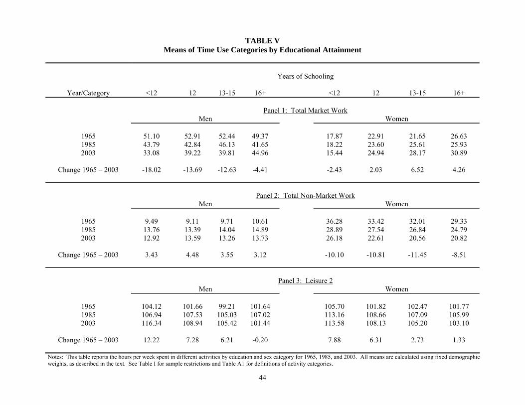
44

TABLE V Means of Time Use Categories by Educational Attainment

Years of Schooling

Year/Category

<12

12

13-15

16+

<12

12

13-15

16+

Panel 1: Total Market Work Men Women

1965 51.10 52.91 52.44 49.37 17.87 22.91 21.65 26.63 1985 43.79 42.84 46.13 41.65 18.22 23.60 25.61 25.93 2003 33.08 39.22 39.81 44.96 15.44 24.94 28.17 30.89

Change 1965 – 2003 -18.02 -13.69 -12.63 -4.41 -2.43 2.03 6.52 4.26

Panel 2: Total Non-Market Work Men Women

1965 9.49 9.11 9.71 10.61 36.28 33.42 32.01 29.33 1985 13.76 13.39 14.04 14.89 28.89 27.54 26.84 24.79 2003 12.92 13.59 13.26 13.73 26.18 22.61 20.56 20.82

Change 1965 – 2003 3.43 4.48 3.55 3.12 -10.10 -10.81 -11.45 -8.51

Panel 3: Leisure 2 Men Women

1965 104.12 101.66 99.21 101.64 105.70 101.82 102.47 101.77 1985 106.94 107.53 105.03 107.02 113.16 108.66 107.09 105.99 2003 116.34 108.94 105.42 101.44 113.58 108.13 105.20 103.10

Change 1965 – 2003 12.22 7.28 6.21 -0.20 7.88 6.31 2.73 1.33

Notes: This table reports the hours per week spent in different activities by education and sex category for 1965, 1985, and 2003. All means are calculated using fixed demographic weights, as described in the text. See Table I for sample restrictions and Table A1 for definitions of activity categories.

45

TABLE VI Differences in Difference in Leisure Measure 2 between 1965 and 2003 by Educational Attainment

Educational Comparison

1985 − 1965

2003 − 1985

Less than High School − College or More 0.49 8.86 High School Graduates − College or More 1.60 4.58 Some College − College or More 0.36 3.41 Notes: This table reports the change in Leisure Measure 2 between 1965 and 1985 (column 1) and 1985 and 2003 (column 2) for all adults with less than high school (row 1), high school (row 2), and some college (row 2), minus the corresponding change over the respective time period for adults with a college education. All differences are calculated using fixed demographic weights, as described in the text.

46

TABLE VII Changes in Leisure 2 1965-2003, Component Breakdown by Education

Years of Schooling

Category

<12

12

12-15

16+

TV 9.31 7.79 6.93 5.48 Sleeping and Personal Care 3.15 1.43 0.67 -1.44 All Other Leisure Measures 2.57 2.04 1.40 0.72 Gardening and Pet Care 1.10 1.52 1.01 1.38 Sports/Sporting Events 0.89 0.68 1.18 1.97 Eating -1.58 -0.04 0.03 1.29 Reading -2.74 -3.16 -2.84 -3.46 Socializing -2.79 -3.52 -4.05 -5.39 All Leisure 2 9.91 6.74 4.33 0.56

Notes: This table reports the change in several sub-categories of Leisure 2 between 1965 and 2003, broken down by educational attainment. All differences are calculated using fixed demographic weights, as described in the text.

47

TABLE VIII Juhn-Murphy-Pierce Decomposition of the Change in the Leisure 2 Distribution

Decomposition

Distribution Percentile Comparison

Total Change

Demographic Quantities

Cell Means

Unobservables

Panel 1. 1965-2003

90-10 14.23 -0.76 2.70 12.29 90-50 9.10 -0.19 0.67 8.63 50-10 5.13 -0.57 2.03 3.67

Panel 2. 1965-1985

90-10 8.75 -1.14 0.57 9.32 90-50 6.53 -0.32 -0.41 7.27 50-10 2.22 -0.82 0.99 2.05

Panel 3. 1985-2003

90-10 5.48 0.38 2.13 2.97 90-50 2.57 0.13 1.08 1.36 50-10 2.92 0.25 1.05 1.62

Notes: This table reports the change in the cross-sectional distribution of Leisure 2 between 1965 and 2003 (Panel 1), between 1965 and 1985 (Panel 2), and between 1985 and 2003 (Panel 3). The cross-sectional distribution is measured by the 90-10 percentile difference (row 1 in each panel), the 90-50 percentile difference (row 2), and the 50-10 percentile difference (row 3). The changes in these percentile comparisons, not adjusting for any demographics, are shown in column 1. The portion of the unadjusted change attributed to changing demographic quantities is reported in column 2. The portion of the unadjusted change attributed to changing demographic cell means is reported in column 3. The last column is the remaining change attributed to unobservables. The details of the methodology are described in the text.

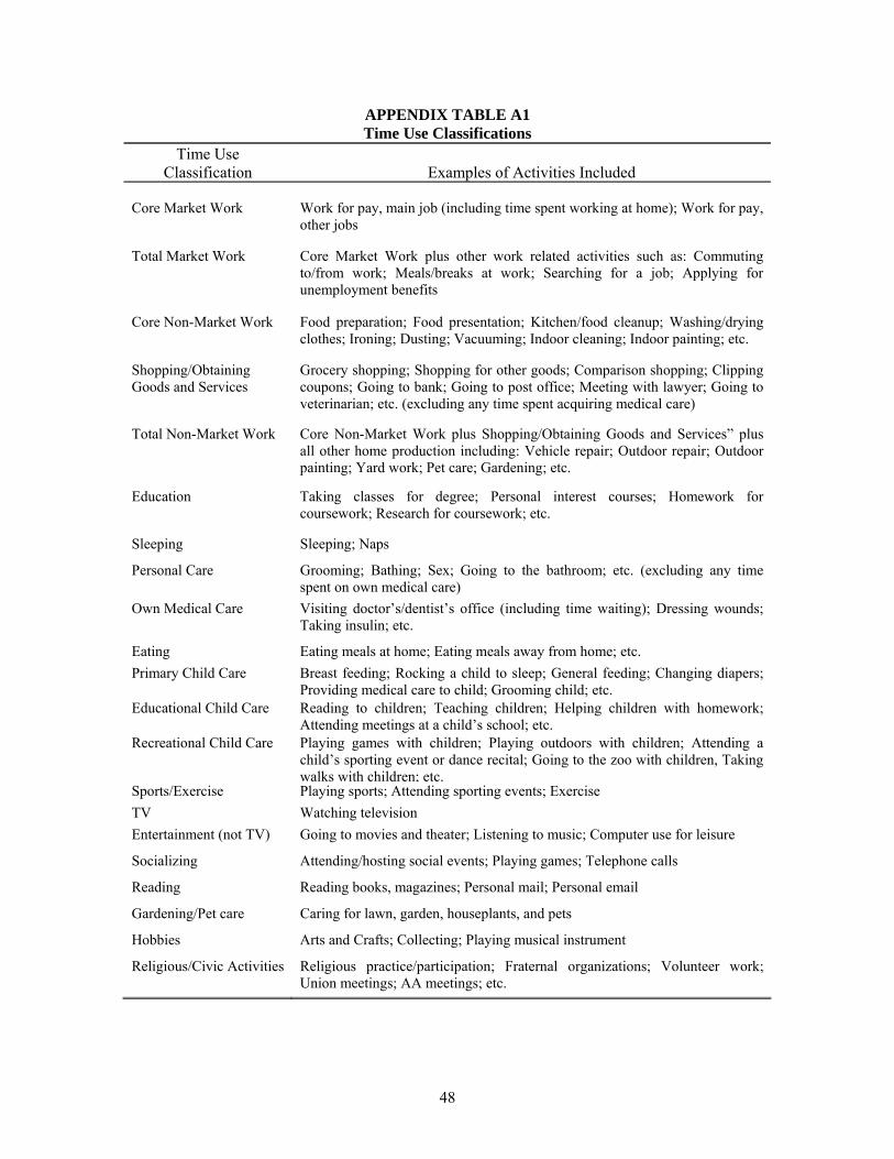
48

APPENDIX TABLE A1 Time Use Classifications

Time Use Classification

Examples of Activities Included

Core Market Work Work for pay, main job (including time spent working at home); Work for pay,

other jobs

Total Market Work Core Market Work plus other work related activities such as: Commuting to/from work; Meals/breaks at work; Searching for a job; Applying for unemployment benefits

Core Non-Market Work Food preparation; Food presentation; Kitchen/food cleanup; Washing/drying clothes; Ironing; Dusting; Vacuuming; Indoor cleaning; Indoor painting; etc.

Shopping/Obtaining Goods and Services

Grocery shopping; Shopping for other goods; Comparison shopping; Clipping coupons; Going to bank; Going to post office; Meeting with lawyer; Going to veterinarian; etc. (excluding any time spent acquiring medical care)

Total Non-Market Work Core Non-Market Work plus Shopping/Obtaining Goods and Services” plus all other home production including: Vehicle repair; Outdoor repair; Outdoor painting; Yard work; Pet care; Gardening; etc.

Education Taking classes for degree; Personal interest courses; Homework for coursework; Research for coursework; etc.

Sleeping Sleeping; Naps

Personal Care Grooming; Bathing; Sex; Going to the bathroom; etc. (excluding any time spent on own medical care)

Own Medical Care Visiting doctor’s/dentist’s office (including time waiting); Dressing wounds; Taking insulin; etc.

Eating Eating meals at home; Eating meals away from home; etc. Primary Child Care Breast feeding; Rocking a child to sleep; General feeding; Changing diapers;

Providing medical care to child; Grooming child; etc. Educational Child Care Reading to children; Teaching children; Helping children with homework;

Attending meetings at a child’s school; etc. Recreational Child Care Playing games with children; Playing outdoors with children; Attending a

child’s sporting event or dance recital; Going to the zoo with children, Taking walks with children; etc.

Sports/Exercise Playing sports; Attending sporting events; Exercise TV Watching television Entertainment (not TV) Going to movies and theater; Listening to music; Computer use for leisure

Socializing Attending/hosting social events; Playing games; Telephone calls

Reading Reading books, magazines; Personal mail; Personal email

Gardening/Pet care Caring for lawn, garden, houseplants, and pets

Hobbies Arts and Crafts; Collecting; Playing musical instrument

Religious/Civic Activities Religious practice/participation; Fraternal organizations; Volunteer work; Union meetings; AA meetings; etc.

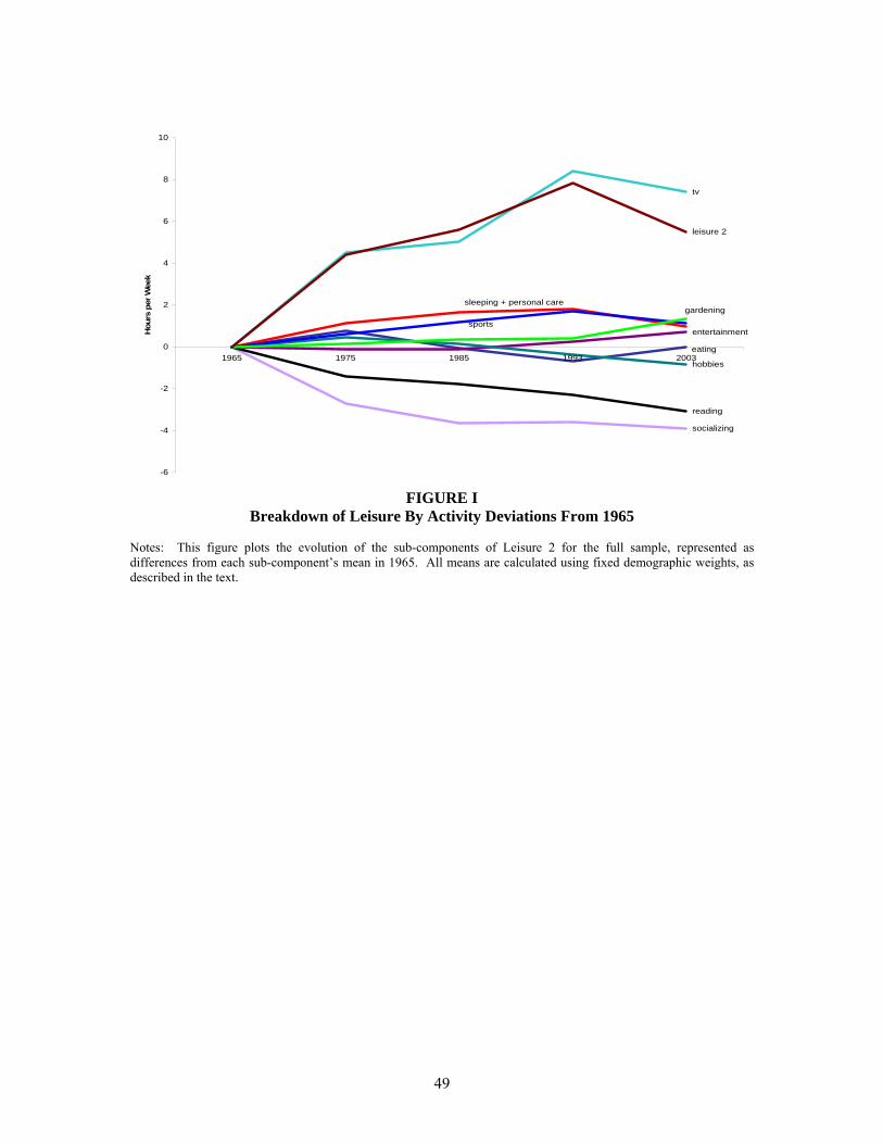
49

tv

socializing

entertainment

hobbies

reading

eating

sleeping + personal care

sports

gardening

leisure 2

-6

-4

-2

0

2

4

6

8

10

1965 1975 1985 1993 2003

Hou

rs p

er W

eek

FIGURE I

Breakdown of Leisure By Activity Deviations From 1965 Notes: This figure plots the evolution of the sub-components of Leisure 2 for the full sample, represented as differences from each sub-component’s mean in 1965. All means are calculated using fixed demographic weights, as described in the text.

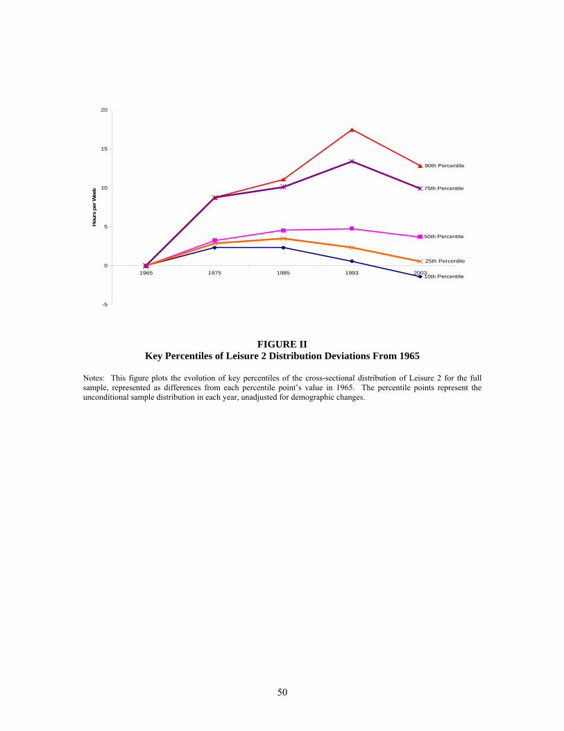
50

10th Percentile

50th Percentile

90th Percentile

25th Percentile

75th Percentile

-5

0

5

10

15

20

1965 1975 1985 1993 2003

Hou

rs p

er W

eek

FIGURE II Key Percentiles of Leisure 2 Distribution Deviations From 1965

Notes: This figure plots the evolution of key percentiles of the cross-sectional distribution of Leisure 2 for the full sample, represented as differences from each percentile point’s value in 1965. The percentile points represent the unconditional sample distribution in each year, unadjusted for demographic changes.

51

-6

-4

-2

0

2

4

6

8

10

12

14

16

5 15 25 35 45 55 65 75 85 95

Percentile of Distribution

Cha

nge

1965

-200

3H

ours

per

Wee

k

FIGURE III Change By Percentile Point For Leisure 2 1965-2003

Notes: This figure plots the change at each percentile point of the Leisure 2 distribution between 1965 and 2003. The percentile points represent the unconditional full-sample distribution in each year, unadjusted for demographic changes.

52

-10

-5

0

5

10

15

20

25

5 15 25 35 45 55 65 75 85 95

Percentile of Distribution

Cha

nge

1965

- 20

03H

ours

per

Wee

k

<12 12 13-15 16+

FIGURE IV Change By Percentile Point For Leisure 2 By Educational Attainment 1965-2003

Notes: This figure plots the change at each percentile point of the Leisure 2 distribution between 1965 and 2003, broken down by educational attainment. The percentile points represent the unconditional distribution of the respective sub-sample in each year, unadjusted for demographic changes.

53

1 In some years, the PSID asks respondents to individually report the amount of time they

spent on household chores during a given week. These data are exploited by Roberts and Rupert

[1995] to document a decline in total work, which, for the overlapping periods, is consistent with

the trends documented in this paper.

2 All time trends discussed in this paper, unless otherwise noted, are adjusted for

changing demographics. See Section II.A for details.

3 Juster and Stafford [1985] fully examined unconditional and conditional time use in the

United States using the 1965 and 1975 time diaries. In the first edition of their book [1997],

Robinson and Godbey extended the analysis of Juster and Stafford by examining the trends in

time use across 1965, 1975, and 1985. In their second edition, Robinson and Godbey added a

chapter entitled “A 1990s Update: Trends Since 1985”. In that chapter, they briefly discuss how

unconditional measures of time in the early 1990s compare with unconditional measures of time

use from earlier decades. However, their discussion does not include the conditional time-use

analysis that is done in this paper. See Schor [1992] for a popular, and controversial, study that

draws different conclusions about the trends in leisure between the mid 1960s and the early

1980s.

4 Because of our reliance on time-use surveys, our paper does not address time allocation

before 1965, the year of the first large-scale, nationally representative time-diary survey for

which micro data are available. Lebergott [1993] is a standard reference for household time use

during the early twentieth century.

5 As opposed to measuring changes in the allocation of time per adult, as we do, Ramey

and Francis [2006] measure changes in the allocation of time per capita. Given that the share of

children in the population has decline sharply during the last forty years, including children in the

per capita measure augments the increase (or mitigates the decrease) for activities that children

spend less time than adults, such as home production and market work. Conversely, given that

54

children have much more free time than adults, any upward trend in leisure per adult that

occurred during the last 40 years will be reduced in per capita terms.

6 The inclusion or exclusion of students from our sample makes little difference to our

results. See Aguiar and Hurst [2006] for trends in time use using an otherwise identical sample

which also includes students.

7 When pooling the surveys together to compute the percent of the population in each of

our cells, we used the weights provided by the surveys to ensure the data is representative of the

total population. Furthermore, we adjusted these weights so that each day of the week and each

survey are equally represented in the overall sample. Given the smaller sample sizes in the early

time use surveys, we do not create our demographic cells so that they are day of week specific,

leaving open the possibility that days of the week are not uniformly distributed within individual

demographic cells. However, in a robustness exercise, we have differentiated respondents by

demographics as well as by whether their diary was completed on a weekend or a weekday.

These results, reported in the robustness appendix available on our websites, were nearly identical

to those reported below.

8 See Aguiar and Hurst [2006] for time trends of key activities without adjustment for

demographics.

9 A discussion of all the time-use categories we use in this paper is found in Appendix

Table A1.

10 For example, using Census data, McGrattan and Rogerson [2004] document an

unconditional decline of 3.6 hours per week for men and an increase of 7.9 hours per week for

women between 1960 and 2000. These values are similar to the change in unconditional means

found in time use data sets. See Table II of Aguiar and Hurst [2006]. However, this paper shows

that these changes are mitigated after adjusting for changing demographics.

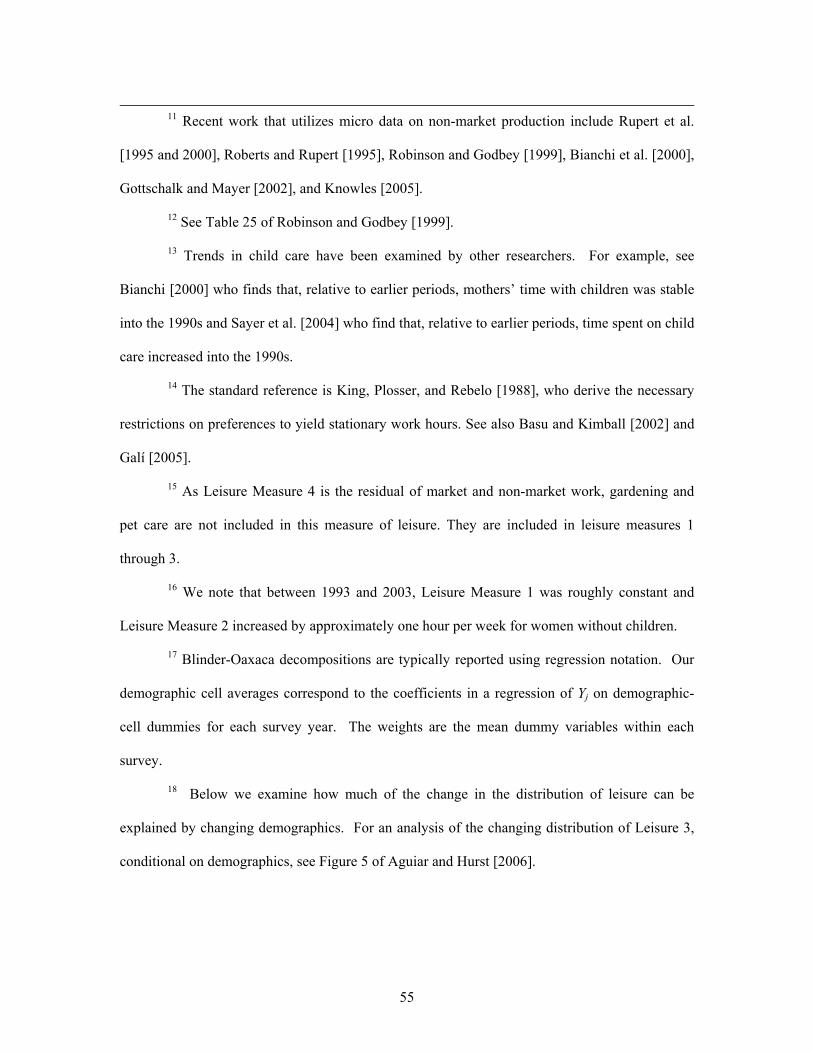
55

11 Recent work that utilizes micro data on non-market production include Rupert et al.

[1995 and 2000], Roberts and Rupert [1995], Robinson and Godbey [1999], Bianchi et al. [2000],

Gottschalk and Mayer [2002], and Knowles [2005].

12 See Table 25 of Robinson and Godbey [1999].

13 Trends in child care have been examined by other researchers. For example, see

Bianchi [2000] who finds that, relative to earlier periods, mothers’ time with children was stable

into the 1990s and Sayer et al. [2004] who find that, relative to earlier periods, time spent on child

care increased into the 1990s.

14 The standard reference is King, Plosser, and Rebelo [1988], who derive the necessary

restrictions on preferences to yield stationary work hours. See also Basu and Kimball [2002] and

Galí [2005].

15 As Leisure Measure 4 is the residual of market and non-market work, gardening and

pet care are not included in this measure of leisure. They are included in leisure measures 1

through 3.

16 We note that between 1993 and 2003, Leisure Measure 1 was roughly constant and

Leisure Measure 2 increased by approximately one hour per week for women without children.

17 Blinder-Oaxaca decompositions are typically reported using regression notation. Our

demographic cell averages correspond to the coefficients in a regression of Yj on demographic-

cell dummies for each survey year. The weights are the mean dummy variables within each

survey.

18 Below we examine how much of the change in the distribution of leisure can be

explained by changing demographics. For an analysis of the changing distribution of Leisure 3,

conditional on demographics, see Figure 5 of Aguiar and Hurst [2006].

56

19 These results are consistent with those documented by Juhn, Murphy and Topel

[2002], which found that starting in the early 1980s low wage men experienced declining hours of

market work relative to high wage men.

20 See the robustness appendix, available on the authors’ web sites, for full details of how

the sample was split.

21 The conclusions are unchanged if we exclude the 1993 survey so as to include a richer

set of controls in our X vector (such as marital status, the number of children and the age of

children).

22 The coefficient vector from a regression like (3.1) in a standard JMP decomposition is

often referred to as “prices” given that the typical application is a wage regression and the

coefficients therefore represent the price of particular attributes represented by X. However, in

our context of leisure time, “cell means” is a more appropriate term for the coefficients on the

dummy variables.

23 See statistics published by Statistics Norway found at

http://www.ssb.no/english/subjects/00/02/20/tidsbruk_en.

Documents

MEASURING TRENDS IN LEISURE: THE ALLOCATION …faculty.chicagobooth.edu/erik.hurst/research/aguiar_hurst_leisure... · MEASURING TRENDS IN LEISURE: THE ALLOCATION OF TIME OVER FIVE