Measuring Trends in Leisure: The Allocation of Time over Five Decades

Mark Aguiar Federal Reserve Bank of Boston

Erik Hurst

University of Chicago, NBER

February 2006

Abstract

In this paper, we use five decades of time-use surveys to document trends in the allocation of time. We find that a dramatic increase in leisure time lies behind the relatively stable number of market hours worked (per working-age adult) between 1965 and 2003. Specifically, we show that leisure for men increased by 6‒8 hours per week (driven by a decline in market work hours) and for women by 4‒8 hours per week (driven by a decline in home production work hours). This increase in leisure corresponds to roughly an additional 5 to 10 weeks of vacation per year, assuming a 40-hour work week. Alternatively, the “consumption equivalent” of the increase in leisure is valued at 8 to 9 percent of total 2003 U.S. consumption expenditures. We also find that leisure increased during the last 40 years for a number of sub-samples of the population, with less-educated adults experiencing the largest increases. Lastly, we document a growing “inequality” in leisure that is the mirror image of the growing inequality of wages and expenditures, making welfare calculation based solely on the latter series incomplete.

JEL Codes: D12, D13, J22

Contact: mark.aguiar@bos.frb.org and erik.hurst@gsb.uchicago.edu. We thank Susanto Basu, Gary Becker, Kathy Bradbury, Kerwin Charles, Raj Chetty, Steve Davis, Jordi Galí, Rueben Gronau, Dan Hamermesh, Chad Jones, Ellen McGrattan, Bruce Mayer, Kevin Murphy, Derek Neal, Valerie Ramey, Richard Rogerson, Frank Stafford, and seminar participants at the Minneapolis Federal Reserve, the Cleveland Federal Reserve (NBER EFG/RSW meeting), the University of Rochester, the University of Wisconsin’s Institute for Poverty Research Summer Institute, NBER Summer Institute in Labor Studies, the University of California at San Diego, the University of California at Berkeley, the University of Chicago, Columbia University, Boston College, Harvard, Wharton, and the University of Maryland. We thank Dan Reichgott for research assistance. Hurst would like to acknowledge the financial support of the University of Chicago’s Graduate School of Business. The views expressed in this paper are solely those of the authors and do not reflect official positions of the Federal Reserve Bank of Boston or the Federal Reserve System.

2

1. Introduction

In this paper, we document trends in the allocation of time over the last 40 years. In

particular, we focus our attention on measuring how leisure time has evolved within the United

States. In commonly used household surveys designed to measure labor market activity (such as

the Current Population Survey (CPS) and the Panel Study of Income Dynamics (PSID)), the only

category of time use that is consistently measured is market work hours.1 As a result, leisure is

almost universally defined as time spent away from market work. However, as noted by Becker

(1965), households can also allocate time towards production outside the formal market sector.

To the extent that non-market (home) production is important and changing over time, leisure

time will be poorly proxied by time spent away from market work. By linking five decades of

detailed time-use surveys, we are able empirically to draw the distinction between leisure and the

complement of market work. In doing so, we document a set of facts about how home production

and leisure have evolved for men and women of differing work status, marital status, and

educational attainment during the last 40 years.

The main empirical finding in this paper is that leisure time—measured in a variety of

ways—has increased significantly in the United States between 1965 and 2003.2 When

computing our measures of leisure, we separate out other uses of household time, including time

spent in market work, time spent in non-market (home) production, time spent obtaining human

capital, and time spent in heath care. Given that some categories of time use are easier to

categorize as leisure than others, we create four distinct measures of leisure. Our measures range

from the narrow, which includes activities designed to yield direct utility, such as entertainment,

socializing, active recreation, and general relaxation, to the broad, namely, time spent neither in

1 In some years, the PSID asks respondents to individually report the amount of time they spent on household chores during a given week. These data are exploited by Roberts and Rupert (1995) to document a decline in total work, which, for the overlapping periods, is consistent with the trends documented in this paper. 2 We provide a formal definition of leisure in Section 3.

3

market production nor in non-market production. While the magnitudes differ slightly, the

conclusions drawn are similar across each of the leisure measures.

Using our preferred definition of leisure, we find that leisure has increased by 7.9 hours

per week on average for men and by 6.0 hours for women between 1965 and 2003, controlling for

demographics. Interestingly, the decline in total work (the sum of total market work and total

non-market work) was nearly identical for the men and women (7.9 and 7.7 hours per week,

respectively). These increases in leisure are extremely large. In 1965, the average man spent 61

hours per week and the average women spent 54 hours per week in total market and non-market

work. The increase in weekly leisure we document between 1965 and 2003 represents 11 to 13

percent of the average total work week in 1965. Valuing time at 2003 market wages, the increase

in leisure has a market value of $5,000 to $5,500 per adult in annual terms. Aggregating over the

adult population, this represents 8 to 9 percent of total GDP in 2003. If we assume the after-tax

market wage represents the marginal rate of substitution between consumption and leisure, to a

first order approximation the increase in leisure is equivalent to 8 to 9 percent of 2003

consumption expenditures.

The adjustments that allow for greater leisure while satisfying the time budget constraint

differ between men and women. Men increased their leisure by allocating less time to the market

sector, whereas leisure time for women increased simultaneously with time spent in market labor.

This increased leisure for women was made possible by a decline in the time women allocated to

home production of roughly 11 hours per week between 1965 and 2003. This more than offset

women’s 5-hours-per-week increase in market labor.3

We also analyze changes in leisure by educational attainment. We find that men and

women with more than a high school education and men and women with a high school education

or less all increased leisure time between 1965 and 2003. However, while the level of leisure in

3 The magnitudes we present in the introduction correspond to changes in time use conditional on demographic changes, as shown in Figures 2–5.

4

1965 was roughly equal across educational status, the subsequent increase in leisure was greatest

among less-educated adults. Similarly, we document that the cross-sectional distribution of

leisure time has fanned out over the last 40 years. Given that the least-educated households

experienced the largest gains in leisure, this growing “inequality” in leisure is the mirror image of

the well-documented trends in income and expenditure inequality. The fact that the least-educated

experience the most leisure poses an empirical puzzle for the standard model that relies solely on

income and substitution effects: The time-series evidence suggests that rising incomes induce

greater leisure, while the recent cross-sections suggest that higher incomes are associated with

lower levels of leisure.

2. Related Literature

Three classic book-length references on the allocation of time are Ghez and Becker

(1975), Juster and Stafford (1985), and Robinson and Godbey (1999). The latter is most closely

related to our study. It uses the same time-use surveys we use from 1965, 1975, and 1985, as well

as some additional time-use information from the early 1990s.4 Our paper adds to the earlier

results of Juster and Stafford and Robinson and Godbey by documenting the growing dispersion

in leisure as well as analyzing a longer time series. We also consider alternative leisure

aggregates. Several other studies have explored the trends in housework, including Bianchi et al.

(2000) and Roberts and Rupert (1995). In addition to extending the sample of Robinson and

Godbey through the late 1990s, the former work contains a nice summary of the existing

sociology literature on housework. The latter uses the market work and housework measures in

the PSID, as does Knowles (2005), who focuses on relative work hours (at home and in the

market) of spouses in younger households. For a popular but controversial study that draws

4 Juster and Stafford (1985) fully examined unconditional and conditional time use in the United States using the 1965 and 1975 time diaries. In the first edition of their book (1997), Robinson and Godbey extended the analysis of Juster and Stafford by examining the trends in time use across 1965, 1975, and 1985. In their second edition, Robinson and Godbey added a short chapter entitled “A 1990s Update: Trends Since 1985”. In that chapter, they briefly discuss how unconditional measures of time in the early 1990s compare with unconditional measures of time use from earlier decades. However, their discussion does not include the conditional time-use analysis that is done in this paper.

5

different conclusions than those of our paper and the papers cited above, see Schor (1992). While

the literature, particularly in sociology, on the allocation of time is large, to the best of our

knowledge, no other study combines the length of time series, the attention to cross-sectional

dispersion (particularly post-1985), and the focus on different measures of leisure found in the

current paper.

Because of our reliance on time-use surveys, our paper does not address time allocation

before 1965, the year of the first large-scale, nationally representative time-diary survey for

which micro data are available. Lebergott (1993) is a standard reference for household time use

during the early twentieth century. See Greenwood, Seshadri, and Yorukoglu (2005) and Ramey

and Francis (2005) for two alternative views regarding the trends in housework during the first

half of the twentieth century. Lastly, Ramey and Francis present evidence on time allocation

spanning the entire twentieth century and draw on the same surveys as we do for the latter half. In

contrast with our study, however, Ramey and Francis analyze the data through the paradigm of a

representative agent to make a direct link to the standard neoclassical growth model. They

therefore do not adjust for changing demographics nor do they focus on cross-sectional

heterogeneity. Given the fact that the share of children in the population has declined

dramatically over the last 40 years, there is a difference between our measure of mean time spent

per adult and Ramey and Francis’s measure of mean time spent per capita. Including children in

the per capita measure augments the increase (or mitigates the decrease) over the last 40 years of

activities in which children spend less time than adults, such as home production and market

work. Conversely, given that children have much more free time than adults, any upward trend in

leisure per adult that occurred during the last 40 years will be reduced in per capita terms.

The present study focuses exclusively on the United States. There are studies that

compare the U.S. and Europe at a point in time (for example, see Freeman and Schettkat 2002

and Schettkat 2003). However, to our knowledge, there are no studies using European data that

6

perform a time-series analysis similar to the one below. This remains an important area for future

research.

3. The Importance of Understanding the Allocation of Time

This paper measures how the allocation of time has evolved over the last 40 years. Before

we begin, it is useful to spend some time discussing why time allocation is important and how it

may influence our understanding of other economic phenomena observed in the market. This

discussion will also help frame the patterns documented in the rest of the paper.

Consider a range of commodities, 1 2, ,..., Nc c c , indexed by n. Utility is defined over

these commodities. Following Becker (1965), each commodity n is produced with a combination

of the household member(s)’ time (hn) and market goods (xn), such that ( , )n n n nc f h x= . For

example, a commodity may be a meal. The inputs are ingredients, time spent cooking, and time

spent eating. Similarly, a commodity may be watching a sporting event on television, which

involves the services of a television set as well as the time spent watching the event.5 In the

Beckerian model, market labor is just one of many uses of time that ultimately produce

consumption commodities.

Viewed in this way, the standard dichotomy between market work and a catch-all term

called “leisure” does not distinguish whether non-market time is spent engaged in cooking or

watching television, to use the above examples. Why is it important to make this distinction? One

primary reason is that economics is the study of how agents allocate scarce resources. How time

is allocated is therefore of interest in and of itself.

Second, and potentially more importantly, if we want to understand the behavior of the

market economy, we need to understand how time is allocated away from the market. This is

important if the elasticity of substitution between time and goods varies across the production

5 See Pollak and Wachter (1975) for a critique based on the fact that the same unit of time may be inputs into multiple commodities. In this section, we abstract from such “joint production” and simply note that this critique is relevant for market time as well.

7

functions for different commodities. Indeed, one definition of whether an activity is “leisure” may

be the degree of substitutability between the market input and the time input in the production of

the commodity. That is, the leisure content of an activity is a function of technology rather than

preferences. In the examples above, one can use the market to reduce time spent cooking (by

getting a microwave or ordering takeout food) but cannot use the market to reduce the time input

into watching television (although innovations like VCRs and Tivo allow some substitution). A

perhaps more ambiguous example would be the commodity of “good health” that requires time

inputs such as doctor visits and medical procedures. We would like to avoid medical visits by

using market substitutes, but we cannot always do so, because of technological constraints.

However, at the margin, one can reduce the waiting time associated with medical care by paying

a market price.

One important application of how the allocation of time away from the market affects

market outcomes is market labor supply. In the Beckerian model, whether a wage increase

draws a worker into the market depends not only on preferences embedded in the utility function

but also on the production functions, nf , as well as on how time is allocated across these

production functions (see Gronau (1977) for an early discussion). If agents are engaged in

activities that have a high degree of substitution between goods and time, they will supply labor

to the market differently in response to a real wage increase than will agents engaged in activities

that have a low elasticity of substitution.

A simple example makes this point explicit. Consider two consumption commodities, 1c

and 2c . These are produced using market goods, x1 and x2, as well as time, h1 and h2, respectively.

The inputs are combined according to a CES production function with elasticity parameters σ and

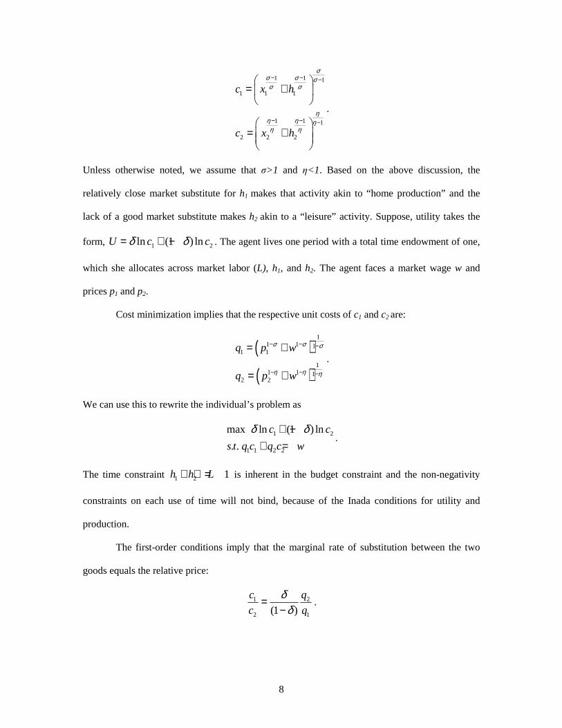
η:

8

1 1 1

1 1 1

1 1 1

2 2 2

c x h

c x h

σσ σ σσ σ

ηη η ηη η

− − −

− − −

= +

= +

.

Unless otherwise noted, we assume that σ>1 and η<1. Based on the above discussion, the

relatively close market substitute for h1 makes that activity akin to “home production” and the

lack of a good market substitute makes h2 akin to a “leisure” activity. Suppose, utility takes the

form, 1 2ln (1 ) lnU c cδ δ= + − . The agent lives one period with a total time endowment of one,

which she allocates across market labor (L), h1, and h2. The agent faces a market wage w and

prices p1 and p2.

Cost minimization implies that the respective unit costs of c1 and c2 are:

( )( )

11 1 1

1 1

11 1 1

2 2

q p w

q p w

σ σ σ

η η η

− − −

− − −

= +

= +.

We can use this to rewrite the individual’s problem as

1 2

1 1 2 2

max ln (1 ) ln

. .

c c

s t q c q c w

δ δ+ −+ =

.

The time constraint 1 2 1h h L+ + = is inherent in the budget constraint and the non-negativity

constraints on each use of time will not bind, because of the Inada conditions for utility and

production.

The first-order conditions imply that the marginal rate of substitution between the two

goods equals the relative price:

1 2

2 1(1 )

c q

c q

δδ

=−

.

9

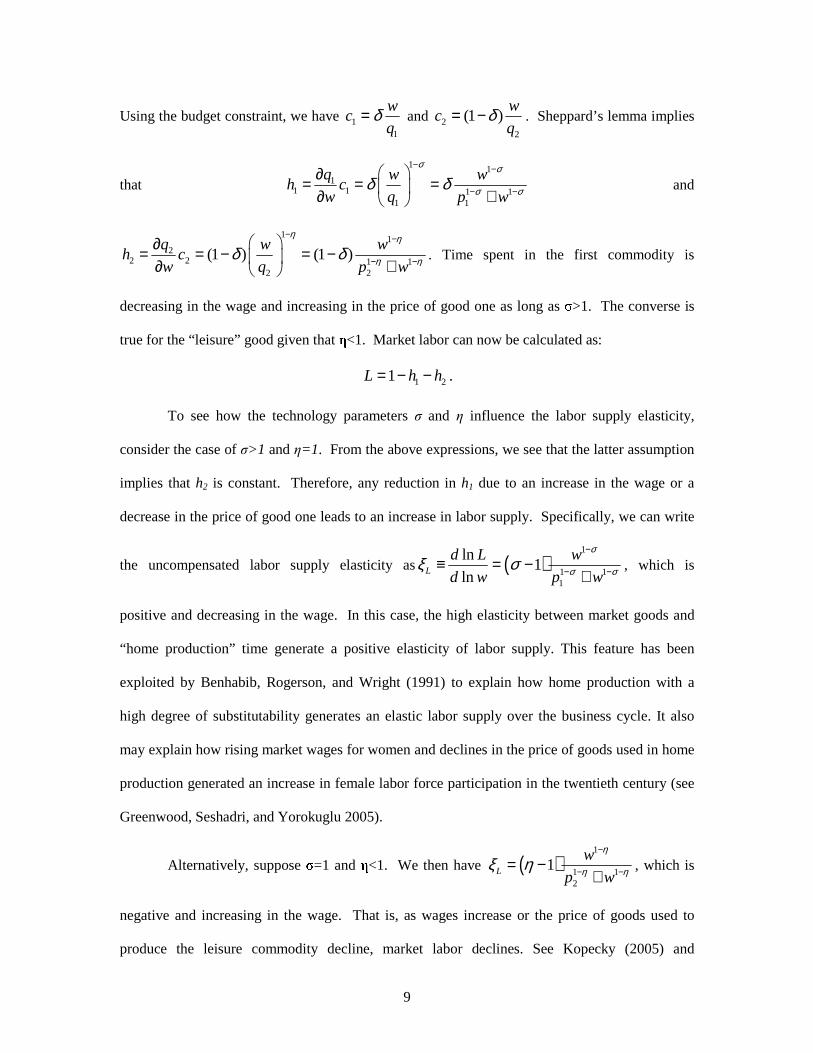
Using the budget constraint, we have 11

wc

qδ= and 2

2

(1 )w

cq

δ= − . Sheppard’s lemma implies

that

1 11

1 1 1 11 1

q w wh c

w q p w

σ σ

σ σδ δ− −

− −

∂= = = ∂ + and

1 12

2 2 1 12 2

(1 ) (1 )q w w

h cw q p w

η η

η ηδ δ− −

− −

∂= = − = − ∂ + . Time spent in the first commodity is

decreasing in the wage and increasing in the price of good one as long as σ>1. The converse is

true for the “leisure” good given that η<1. Market labor can now be calculated as:

1 21L h h= − − .

To see how the technology parameters σ and η influence the labor supply elasticity,

consider the case of σ>1 and η=1. From the above expressions, we see that the latter assumption

implies that h2 is constant. Therefore, any reduction in h1 due to an increase in the wage or a

decrease in the price of good one leads to an increase in labor supply. Specifically, we can write

the uncompensated labor supply elasticity as ( )1

1 11

ln1

lnL

d L w

d w p w

σ

σ σξ σ−

− −≡ = −+

, which is

positive and decreasing in the wage. In this case, the high elasticity between market goods and

“home production” time generate a positive elasticity of labor supply. This feature has been

exploited by Benhabib, Rogerson, and Wright (1991) to explain how home production with a

high degree of substitutability generates an elastic labor supply over the business cycle. It also

may explain how rising market wages for women and declines in the price of goods used in home

production generated an increase in female labor force participation in the twentieth century (see

Greenwood, Seshadri, and Yorokuglu 2005).

Alternatively, suppose σ=1 and η<1. We then have ( )1

1 12

1L

w

p w

η

η ηξ η−

− −= −+

, which is

negative and increasing in the wage. That is, as wages increase or the price of goods used to

produce the leisure commodity decline, market labor declines. See Kopecky (2005) and

10

Vandenbroucke (2005) for models that exploit this feature to explain declining work hours over

the twentieth century. Greenwood and Vandenbroucke (2005) provide a nice synthesis of these

models in the context of long-run trends in market labor.

In the more general case of σ>1 and η<1, the response of labor supply to wage and price

changes depends on preferences and technology. Indeed, the symmetric case of δ=1-δ, p1=p2,

and σ-1=1-η generates constant market work hours backed by a decline in h1 (home production)

and an increase in h2 (leisure). At least qualitatively, this is not far removed from the data

presented for the average household in the next section.

The above example, albeit stylized, makes it clear that the way that agents allocate their

time away from the market has a direct bearing in understanding market labor supply. In

particular, it makes a difference whether non-market activities have close market substitutes or

not. Such an accounting may also guide our understanding of why labor supply elasticities change

over time and across sub-groups (see, for example, Juhn and Murphy 1997), why hours and

employment vary, and how technological shocks in the production of home goods or in the

production of market goods influence total output. For example, if women are more likely to

allocate their non-market time to home production, the analysis suggests that women will have

higher elasticities of labor supply than men (see Mincer 1962).

Moreover, understanding time allocation is important in distinguishing actual

“consumption” from market expenditure (see Aguiar and Hurst 2005a, 2005b).6 Ignoring the

allocation of time may generate an incomplete view of the welfare consequences of changes in

expenditure. The evidence presented below suggests that this is particularly important in

understanding the welfare consequences of wage and expenditure inequality in the U.S.

Specifically, the well-documented increase in the relative wages and expenditures of educated

individuals (Katz and Autor 1999, Attanasio and Davis 1996, Krueger and Perri, forthcoming) is

6 Exploring a different margin of substitution, Cutler et al. (2003) use the intuition of the above home production technology to show that the increased convenience of manufactured foods explains a significant portion of the observed increase in U.S. obesity rates.

11

shown below to be accompanied by little change in the relative time spent in home production but

a large decline in the relative time spent in leisure.

Overall, the patterns described below will help to guide the choice of parameters for the

utility and home-production functions in calibrated models. Specifically, the traditional

motivation for utility functions that display off-setting income and substitution elasticities for

labor supply has been the relatively stable market-work hours per adult observed in the post-war

economy (Prescott 1986). This has been interpreted as reflecting a constant level of leisure, which

is shown below not to be the case. Moreover, the steady decline in home production time over the

last 40 years argues for a high elasticity of substitution between time and goods in home

production, constant technological improvement in home production, or a combination of the

two.

4. Empirical Trends in the Allocation of Time

To document the trends in the allocation of time over the last 40 years, we link five major

time use surveys: 1965-1966 America’s Use of Time; 1975-1976 Time Use in Economics and

Social Accounts; 1985 Americans’ Use of Time; 1992-1994 National Human Activity Pattern

Survey; and the 2003 American Time Use Survey. The Data Appendix and Table 1 describe these

surveys in detail. In this section, we characterize four major uses of time: market work, non-

market production, child care, and “leisure.”

We take two approaches to document trends over the last 40 years. The first is to report

the (weighted) means from the time-use surveys for each activity.7 Throughout the analysis, we

restrict our sample to include only non-retired individuals between the ages of 21 and 65, so these

averages are “per working-age adult” (or per adult within the specified sub-sample, when

relevant). We drop adults younger than 21 and adults older than 65 (as well as early retirees) to

7 When reporting either the unconditional or conditional means, we weight the time-diary data using the weights provided by the surveys. Furthermore, we adjust the weights so that each day of the week and each survey is equally represented for the full sample of individuals.

12

minimize the role of time allocation decisions that have a strong inter-temporal component, such

as education and retirement. Moreover, the 1965 time-use survey excludes households with heads

who are either retired or over the age of 65. So, to create consistent samples across the years, we

need to omit these households. Omitting an analysis of retirees will likely imply that the increase

in leisure that we document is an underestimate of the actual increase in leisure for adults, given

that individuals are living longer and spending a larger fraction of their life in retirement.

Additionally, the 1965, 1975, and 1985 time-use surveys exclude individuals under the age of 18

or 19 from their samples.

The second approach we take is to condition the change in time spent in various activities

on demographics. During the last 40 years, there have been significant demographic changes in

the U.S. This is evident from the data shown in Appendix Table A1, which describes the

demographic composition of the time-diary samples. Since 1965, the average American has aged,

become more educated, become more likely to be single, and had fewer children. All of these

changes may affect how an individual chooses to allocate his or her time. For example,

historically, individuals in their late 50s spend less time in market work than individuals in their

early 40s. It would not be surprising to see that time spent in market work per working-age adult

has fallen during the last 40 years simply because the fraction of 50-year-olds relative to 40-year-

olds has increased.

By conditioning on these demographics, we are reporting how time spent in a given

activity has changed during the last 40 years adjusted for demographic changes. Formally, we

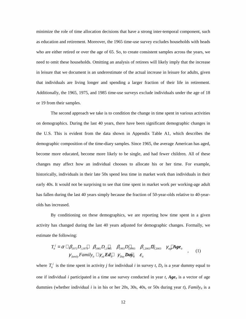
estimate the following:

1975 ,1975 1985 ,1985 1993 ,1993 ,2003 ,2003

jit i i i i i age it

family it ed it Day it it

T D D D D

Family

α β β β β γγ γ γ ε

= + + + + + +

+ + +

Age

Ed Day, (1)

where jitT is the time spent in activity j for individual i in survey t, Dit is a year dummy equal to

one if individual i participated in a time use survey conducted in year t, Ageit is a vector of age

dummies (whether individual i is in his or her 20s, 30s, 40s, or 50s during year t), Familyit is a

13

dummy variable equaling one if respondent i has a child, Edi is a vector of education dummies

(whether i completed 12 years of schooling, 13-15 years of schooling, or 16 or more years of

schooling in year t), and Dayit is a vector of day of week dummies. The day-of-week dummies are

necessary, given that some of the surveys over sample weekends for some sub-samples.

The coefficients on the year dummies describe how average time spent on an activity has

changed over time, controlling for changes in key demographics.8 In all years except 1993, the

time-use surveys asked respondents to report their marital status and the number of children that

they had. Although our base results do not include these controls (because they are unavailable in

1993), we reran all of our regressions including marital status and the number of children as

additional controls on a sample that excludes the 1993 survey. We also performed robustness

checks by including dummies to indicate the age of the youngest child and to indicate whether the

individual was working part-time. These modifications did not alter the main findings of our

paper.

4.1 Trends in Market Work

Trends in market work over the last half century have been well documented (see, for

example, McGrattan and Rogerson 2004). The major difference between our results and those

using traditional household surveys such as the CPS and PSID is that our research focuses on

changes in the allocation of household time across market work, non-market work, and leisure,

while the existing research tends to focus exclusively on changes in market hours. As we show in

this paper, the conclusions about changing leisure drawn solely from time spent working in the

market sector are misleading. Moreover, it has been well documented that such surveys tend to

over-report market work hours relative to time diaries (see Juster and Stafford 1985 and Robinson

and Godbey 1999). Given the propensity for individuals to provide focal point answers in

8 Notice, when reporting the coefficients on the year dummies from a regression such as (1), we are controlling for both trends in demographics over time and for the fact that the time-use surveys may not be nationally representative with respect to the demographic controls included in the regression during a given individual year even after weighting.

14

household surveys such as the PSID, CPS, or Census, it has been shown that time diaries provide

a more accurate measure of the actual time an individual spends working, given that total time

allocation must sum to 24 hours. As a validation exercise, in the Data Appendix, we provide a

detailed comparison of the PSID market-work hours with market-work hours reported within the

time diaries and argue that while there is a level shift between the two types of surveys, the trends

are broadly consistent across them.

We define market work in two ways. “Core” market work includes all time spent

working in the market sector on main jobs, second jobs, and overtime, including any time spent

working at home.9 This market-work measure is analogous to the market work measures in the

Census, the PSID, or the Survey of Consumer Finances (SCF). The broader category “total”

market work is core market work plus time spent commuting to/from work and time spent on

ancillary work activities (for example, time spent at work on breaks or eating a meal).

The unconditional means of core market work and total market work for men and women

during each time-use survey are shown in Table 2. Given the broad similarity in trends between

the unconditional and the conditional means, we focus our discussion on the means that are

conditional on demographics. In Figure 1, we plot the conditional changes in hours per week

relative to 1965 for all adults as well as for men and women separately. Average hours per week

of core market work for working-age adults were essentially constant between 1965 and 2003.

However, as is well known, this relatively stable average masks the fact that market-work hours

for men have fallen and market-work hours for women have increased sharply. Specifically, after

adjusting for changing demographics, core market-work hours for males fell by 6.4 hours per

week between 1965 and 2003 (p-value < 0.01).10 As seen in Figure 1, the entire decline in core

market work hours for men occurred between the 1965 and 1985 surveys. This pattern is also

evident in large household surveys such as the PSID (Appendix Figure A1).

9 A discussion of all the time-use categories we use in this paper is found in Appendix Table A2. 10 The associated point estimates and robust standard errors for all figures shown in this paper are reported in Appendix Tables A3 and A4.

15

Female core market-work hours, conditional on demographic changes, increased by 4.6

hours per week (p-value <0.01). The increase in core market-work hours for women occurred

continuously between 1965 and 1993, before stabilizing in the last decade. These trends in male

and female labor force participation and work hours have been well documented in the

literature.11

The decline in market work for men is relatively larger using our broader measure of

“total market work.” Specifically, total market work declined by 11.6 hours per week, as opposed

to 6.3 hours per week for core work. The difference stems primarily from a decline in breaks at

work, perhaps reflecting the decline over this period in unionized manufacturing jobs in which

breaks are clearly delineated. For women, the increase in total market work was slightly smaller

than the increase in core market work (3.0 vs. 4.2 hours per week, p-value <0.01).

4.2 Trends in Non-Market Work

Unlike the trends in time spent in market work, the trends in time spent in “non-market”

work between 1965 and 2003 have been relatively unexplored.12 We define three categories of

time spent on non-market production. Throughout the paper, time spent on an activity includes

any time spent on transportation associated with that activity.

First, we define time spent on “core” housework. Broadly, this includes any time spent on

meal preparation and cleanup, doing laundry, ironing, dusting, vacuuming, indoor household

cleaning, indoor design and maintenance (including painting and decorating), etc. Second, we

analyze time spent “obtaining goods and services.” This category includes all time spent

acquiring any goods or services (excluding medical care, education, and restaurant meals).

Examples include grocery shopping, shopping for other household items, comparison shopping,

coupon clipping, going to the bank, going to a barber, going to the post office, buying goods on-

11 For example, using Census data, McGrattan and Rogerson (2004) document an unconditional decline of 3.6 hours per week for men and an increase of 7.9 hours per week for women between 1960 and 2000. These values are similar to the change in unconditional means we report in Table 2. 12 Recent work that utilizes micro-data on non-market production include Rupert, Rogerson, and Wright (1995 and 2000), Robinson and Godbey (1999), Roberts and Rupert (1995), and Bianchi et al. (2000).

16

line, etc. The last category we analyze is “total non-market work” which includes time spent in

core household chores, time spent obtaining goods and services, plus time spent on other home

production such as home maintenance, outdoor cleaning, vehicle repair, gardening, pet care, etc.

This latter category is designed to be a complete measure of non-market work. Note that we

separately discuss and analyze time spent in child care in Section 4.4.

The unconditional trends in non-market work are shown in Table 2, panel A (full

sample), panel B (males), and panel C (females). While total market work hours for the full

sample have been relatively constant over the last 40 years, time spent in non-market work has

fallen sharply. Specifically, time spent in food preparation and indoor household chores has fallen

by 6.4 hours per week, time spent obtaining goods and services has fallen by 0.8 hour per week,

and total non-market work has fallen by 5.5 hours per week (p-value of all declines <0.01).

As with market work hours, the average trends mask differences across sexes. Male non-

market work hours have actually increased by 3.9 hours per week (p-value <0.01). Female non-

market work hours have fallen by almost 12.6 hours per week (p-value <0.01).

Figure 2 shows the change (conditional on demographics) in total non-market work hours

between 1965 and 2003 for the full sample and then separately for men and women. The results,

conditional on demographics, mimic the unconditional means displayed in Table 2. In the

aggregate, total non-market work fell by 4.6 hours per week (p-value <0.01). For males, total

non-market work increased by 3.7 hours per week and for females, total non-market work fell by

11.1 hours per week (p-value of both <0.01).

Disaggregating the changes in time spent on non-market work into its three components,

we find that for women, time spent on “core” housework decreased by 10.1 hours per week and

time spent obtaining goods and services decreased by 1.4 hours per week (p-value of both <0.01).

Women slightly increased time spent on other non-market work by 0.5 hours per week (p-value =

0.30). For men, time spent on “core” housework increased by 1.4 hours per week and time spent

on other non-market work increased by 2.9 hours per week (p-values of both < 0.01). Men,

17

however, experienced a decline in time spent obtaining goods and services of 0.6 hours per week

(p-value = 0.14).

4.3 Trends in Total Work

We combine total market work with total non-market work to compute a measure of

“total work.” Table 2 documents the unconditional changes in total work between 1965 and 2003.

Likewise, Figure 3 shows the evolution of total work conditional on demographics.

For the full sample and unconditional on demographics, total work has fallen by 6.8

hours per week (p-value <0.01). A striking result is that the decline in total market work is nearly

identical between men and women. Between 1965 and 2003, conditional on demographics, males

and females decreased their total work hours by 7.9 and 7.7 hours per week, respectively (p-value

of both <0.01).13 The similarity is surprising, given the increase in the relative wage of women

over this period and the simultaneous increase in the market work hours of women. This places a

strong restriction on theories explaining the increase in female labor force participation.

Notice that the results in Table 2 and Figure 3 provide a dramatically different picture for

the evolution of time allocation than one usually infers from examining standard household

surveys that measure only time spent in market work. Specifically, the dramatic increase in the

market work hours of women masks a decline in total work hours. Conditional on demographics,

women have experienced a decline of over 11 hours per week in the time they spend on home

production—an amount that is nearly three times as large as their conditional increase in time

spent in market work. In other words, for women, changes in market work reveal little about

changes in total work.

Another important consideration raised by the trends in total work hours is whether the

economy is on a balanced growth path. Taken as a whole, the strong downward trend in total

work (market plus non-market work) suggests that the economy may not be on a balanced growth

13 The decline in total work is slightly mitigated for men if we also condition on marital status (hence omitting the 1993 survey), as well as on the number of children in the household and whether the youngest child is younger than four. Specifically, total work fell by 6.9 hours per week for men and 7.6 hours per week for women between 1965 and 2003.

18

path, although this does not rule out the possibility that the economy may asymptote to such a

path. The relatively stable figure for market-work-hours per adult over the last 40 years (in the

presence of steady increases in real incomes) is often used to justify utility functions in which the

income and substitution effects of wage changes cancel.14 If non-market work yields a disutility

similar to that of market work, the downward trend in the sum of these variables suggests that this

assumption is inappropriate.

4.4 Trends in Child Care

We should note that none of our measures of non-market work includes child care, which

we argue may be inherently distinct from housework in terms of utility and the elasticity of

substitution between time and market goods. While many aspects of child care have direct market

substitutes, this does not necessarily imply that at the margin parental time and market goods

have a high elasticity of substitution. There are certain elements of child rearing for which

market goods and parental time are not good substitutes. This proposition is supported by the fact

that hardly anyone uses market substitutes to raise their children completely. For this reason, we

feel it appropriate to analyze child care separately.

Moreover, from the standpoint of empirical implementation, there appears to be a

discontinuity in how child care is measured between the 2003 ATUS and all other surveys. The

BLS has explicitly stated that collecting accurate measures of time inputs into child development

is a primary goal of the ATUS. This emphasis is reflected in the fact that the BLS tracks who is

present during every activity recorded. As a result, there is a potential for there to be an increase

in time spent in child care activities between the 2003 time-use survey and the other surveys that

results purely from a change in the classification of activities across the surveys. Time spent in

activities that were conducted in the presence of children that were previously coded as time

spent in other activities may have been classified as child care in 2003. It should be noted that this

14 The standard reference is King, Plosser, and Rebelo (1988), who derive the necessary restrictions on preferences to yield stationary work hours. See also Basu and Kimball (2002) and Galí (2005).

19

measurement issue should not be problematic for activities where children were not present, such

as market work or non-market work during the day, when children are at school.

Table 3 shows a large increase in time spent in child care in the 2003 survey relative to

all other surveys. We define “primary” child care as any time spent on the basic needs of

children, including breast feeding, rocking a child to sleep, general feeding, changing diapers,

providing medical care (either directly or indirectly), grooming, etc. Note that time spent

preparing a child’s meal is included in general “meal preparation,” a component of non-market

production. We define “educational” child care as any time spent reading to children, teaching

children, helping children with homework, attending meetings at a child’s school, etc. We also

define “recreational” child care as playing games with children, playing outdoors with children,

attending a child’s sporting event or dance recital, going to the zoo with children, and taking

walks with children. Lastly, we examine “total child care,” which is simply the sum of the other

three measures.

In Table 3, we show the unconditional evolution of hours per week spent in all four of

these child-care measures for three different groups: working females, non-working females, and

all males. We define working as those employed, regardless of whether the job is full time or part

time. Moreover, these samples are not conditioned on whether a child is present in a household.

In essence, we have pooled together households with and without children. Notice that for

working women, the time they spent on all measures of child care was nearly constant between

1965 and 1993 (panel A). This occurred despite the fact that the incidence of having a child for

this sub-sample fell from 46 percent in 1965 to roughly 38 percent in 1993. Moreover,

conditional on having a child, the number of children in the household fell slightly, from 2.3 to

1.8, between 1965 and 2003, for working women. Despite a relatively constant amount of time

allocated to child care between 1965 and 1993, there was a 2.6-hours-per-week increase in

reported time spent on child care by working women between 1993 and 2003. This recent

increase in time spent in child care occurred in all categories: Time spent on primary child care

20

increased by 1.7 hours per week, time spent on educational child care increased by 0.5 hours per

week, and time spent on recreational child care increased by 0.4 hours per week. A similar pattern

is observed for non-working women (panel B) and all men (panel C). Furthermore, similar

patterns exist for men and women of differing levels of education (not shown).

While the increase in child care between 1993 and 2003 may have resulted from an actual

change in household behavior, it also likely that this increase is simply an artifact of the emphasis

that the 2003 data placed on collecting the amount of time individuals spend in child care.15 To

explore this concern, we used data from the 1997 and 2002 Child Development Supplements

(CDS) of the PSID. These supplements focused on the measurement of many activities related to

the children of the PSID respondents. As part of the CDS, time diaries were administered to the

children in the sample. So, instead of having time diaries of parents, we have time diaries of the

children. These children were asked to report whether a parent or caregiver was actively

participating in each of the activities recorded in the time diary. Time spent with fathers and

mothers was recorded separately. If the increase in child-care activities documented in the 2003

BLS time-use study (relative to the other time-use studies) were real, we would expect to find a

similar increase in parental time spent actively engaged in the child’s activities between the 1997

and 2002 PSID Child Development Survey. However, no large increase was found. Depending on

the specification, the PSID data are consistent with an increase in parental time spent with

children of between zero and one-half hour per week between the mid 1990s and early 2000s.

However, using the consistently measured PSID data, there is no evidence that child care

increased by more than one-half hour per week between 1997 and 2003.

This potential inconsistency in measurement can pose a problem for our analysis, given

that, as we noted above, these time-use data sets ensure that the daily time budget constraint is

met. If the 2003 time-use survey is over-estimating the amount of time individuals spend in child

15 See also Bianchi (2000), who finds that mothers’ time with children was stable into the 1990s. Sayer et al. (2004) find an increase in child care in the late 1990s. However, similar to the ATUS, the 1998 survey used in that study also was designed to measure time with children.

21

care relative to the previous surveys, the 2003 survey must, by definition, be under-representing

the amount of time that the individual is spending in other activities relative to the earlier surveys.

However, as noted above, this change in measurement affects only those activities in which a

child is present. For this reason, in the following section we create multiple measures of leisure

that alternatively include and exclude child care.16 Additionally, in Section 6, as a further

robustness check, we examine the changes in time use for individuals without children.

To provide some context for whether the omission of child care from work drives the

downward trend in total work, we define an alternative measure of non-market work that equals

our benchmark measure plus all child care activities. Conditional on demographics, this measure

of total non-market work fell by 9.2 hours per week for women and increased by 5.5 hours per

week for men. The corresponding changes for total work are a 5.8 hour per week decline for

women and a 6.1 hour per week decline for men.

4.5 Trends in Leisure

We argued in Section 3 that one definition of “leisure” is as a characterization of

technology, that is, how substitutable are time and goods in the production of the ultimate

consumption commodity. This definition is empirically problematic in that we typically do not

have independent measures of the underlying “production” functions or their outputs. A

commonly used alternative definition of leisure is as a residual of total work. Under this

definition, the results just discussed suggest that, conditional on demographics, leisure increased

by roughly 8 hours per week for men and women. As a broad benchmark, we include this

measure below as “Leisure Measure 4.” However, this measure includes activities that have

market substitutes. For example, time spent on education is an investment in human capital that

16 While less conceptually ambiguous, a similar measurement issue applies to care for other adults (that is, care for older or sick parents or grandparents). The 2003 ATUS survey has over 25 different time-use codes concerning care for household and non-household adults compared with a single “time spent at help and care” code in previous surveys. This corresponds to an increase of over one hour per week spent on “other care” between 1993 and 2003, with essentially no change between 1965 and 1993. Due to this complication, we also exclude care for other adults from our measure of non-market work.

22

generates additional consumption goods in the future. Or, at some level, sleep is a biological

necessity that is an input into productivity during the day rather than pure leisure (see, for

example, Biddle and Hamermesh 1990).

At the other extreme, we could define leisure as activities for which the time input is

essential in the sense that the activity itself provides utility (although the time may be paired with

complementary market goods). Examples include watching television or playing golf. This is

arguably more keeping with the “low elasticity” approach advocated in Section 3.

Rather than try to resolve this debate on theoretical grounds, we proceed by exploring

three alternative definitions of leisure. Indeed, it turns out that our various measures tell a fairly

consistent story regarding the past 40 years, making much of the ambiguity of what actually

constitutes leisure empirically unimportant. Indeed, we show below that much of the trend in our

four leisure measures is driven by our narrowest measure. The unconditional means of our four

Leisure Measures are reported in Table 4, and the changes relative to 1965 conditional on

demographics are depicted in Figure 4.

Our first alternative measure of leisure, “Leisure Measure 1,” sums together all time

spent on “entertainment/social activities/relaxing” and “active recreation.” We consider that

activities in this measure do not have close market substitutes (although they often involve

complementary market goods). The lack of market substitutes is due to the fact that the activities

themselves are pursued solely for direct enjoyment. These activities include television watching,

leisure reading, going to parties, relaxing, going to bars, playing golf, surfing the web, visiting

friends, etc. In this leisure measure, we include a subset of child care. Namely, we include

“recreational” child-care activities such as playing with a child, going on outings with a child,

attending a child's sporting events or dance recital, etc.

23

We include gardening and time spent with pets in our alternative leisure measures. This is

the only set of activities that is classified as both leisure and home production.17 Pet care is akin to

playing with children in the sense that it provides direct utility but is also something one can

purchase on the market. Conceptually, gardening is more likely to be considered a hobby, while

cutting grass and raking leaves is more likely to be seen as work (of course, this is subject to

debate). However, the data do not let us draw the distinction between gardening and yard work

consistently throughout the sample. In the pre-2003 surveys, yard work is included in outdoor

home maintenance, while gardening is a separate activity. Unfortunately, in 2003, yard work is

not differentiated from gardening. The result is that the combined pet care and gardening category

increases roughly 30 minutes per week between 1965 and 1993, and then increases a little more

than one hour per week between 1993 and 2003.

As seen in Figures 4a through 4c, Leisure Measure 1 increased by 5.1 hours per week for

the full sample— by 6.4 hours per week for men and 3.8 hours per week for women (p-value for

all <0.01). Leisure 1 increased fairly consistently for men between 1965 and 2003. However, for

women, leisure 1 increased monotonically between 1965 and 1993 and then declined between

1993 and 2003. As we will show later, the entire decline between 1993 and 2003 can be

explained by the increase in child care in this interval, further suggesting that child care is

measured differently in the 2003 survey. However, regardless of such measurement issues, our

basic measure of leisure increased dramatically for both men and women between 1965 and 2003.

Biddle and Hamermesh (1990) argue that certain time activities may enhance production

in the market and non-market sectors. For example, they provide a model in which time spent

sleeping is a choice variable that both augments productivity and enters the utility function

directly. Furthermore, they provide strong empirical evidence showing that sleep time is, in fact, a

choice variable over which individuals optimize. For example, individuals sleep more on the

17 As leisure measure 4 is the residual of market and non-market work, gardening and pet care are not included in this measure of leisure. They are included in leisure measures 1 through 3.

24

weekends and on vacations. Similar conceptual points apply broadly to time spent eating and on

personal care. In this spirit, we define Leisure Measure 2 as activities that provide direct utility

but may also be viewed as intermediate inputs. Specifically, Leisure Measure 2 includes Leisure

Measure 1 as well as time spent in sleeping, eating, and personal care. While we exclude own

medical care,18 we include such activities as grooming, having sex, sleeping or napping, eating at

home or in restaurants, etc.

Conditional on demographics, Leisure Measure 2 increases by 5.6 hours per week (p-

value <0.01) between 1965 and 2003. In other words, in addition to the increase in Leisure

Measure 1, time spent in sleeping, eating, and personal care increased by an additional 30 minutes

per week between 1965 and 2003 (p-value <0.01). Conditional on demographics, time spent in

Leisure Measure 2 increased by 6.4 hours per week for men and by 4.9 hours per week for

women, relative to 1965 (p-value of both <0.01). Note that the comparable numbers for the

changes in Leisure Measure 1 were 6.4 hours per week for men and 3.8 hours per week for

women. As a result, of the total increase in Leisure Measure 2 between 1965 and 2003, the share

accounted for by sleeping, eating, and personal care, was essentially 0 percent for men and 29

percent for women.

Our final alternative leisure category, “Leisure Measure 3,” includes Leisure Measure 2

plus time spent in “primary” and “educational” child care. Recall that “recreational” child care

was included in Leisure Measure 1. The inclusion of child care has very little effect on trends

between 1965 and 1993, but it does make a difference regarding the change over the last decade.

As discussed above, one should be careful in interpreting the change in child care between the

prior surveys and the 2003 survey. Leisure 3 increased by 6.9 hours per week for the full

sample—by 7.9 hours per week for men and 6.0 hours per week for women.

18 Medical care conceptually provides no direct utility and, at the margin, the time spent on a doctor’s visit can be reduced for a price.

25

As noted above, “Leisure Measure 4” is the residual of total work. The difference

between Leisure Measures 3 and 4 includes time spent in education, civic and religious activities

(going to church, volunteering, social clubs, etc.), caring for other adults, and own medical care.

Between 1965 and 2003, civic activities fell by 30 minutes per week, education and own medical

care increased by roughly 30 minutes each, and care for other adults increased by one hour per

week (all of the latter increase taking place between the last two surveys, as discussed in Section

4.4).

In short, controlling for demographics, since 1965 leisure has increased by 5.1 hours per

week (Leisure Measure 1) to 6.9 hours per week (Leisure Measure 3) for the average non-retired

adult. It should be stressed that these magnitudes are economically large. In 1965, the average

individual spent 29 hours per week in core market work (roughly 4 hours per day). The gain in

total leisure between 1965 and 2003 is therefore equal to between 1.2 and 1.7 work-days per 1965

core market work week. Or, if one assumes a 40-hour work week, the increase in leisure is

equivalent to 6.6 to 9.0 additional weeks of vacation per year.

Also, we should note that the increase in Leisure Measure 3 has been essentially

monotonic over the last 40 years for both men and women (with the one caveat concerning child

care). This suggests that the increase in Leisure Measure 3 is not due to differences in

measurement across the five time-use surveys. It is unlikely that each successive survey became

more likely to classify a given activity as being leisure as opposed to work. Moreover, while

roughly one-half of the increase in Leisure Measure 3 occurred between 1965 and 1975

(reflecting, in part, a recession), since 1975, the data suggest continued increases in leisure for

both men and women.

Finally, there are three reasons to believe that the increase in leisure that we have

documented may be biased downwards. First, we are measuring changes in leisure only for non-

retired individuals (given our data limitations). But, the fact that individuals are living longer and

are retiring earlier, coupled with the fact that retired individuals enjoy more leisure than non-

26

retired households (Hamermesh 2005), implies that the increase in lifetime leisure is much larger

than we document.

Second, there has been a claim that the nature of time spent at work has changed over the

last decade. While at work, individuals may engage in more leisure-type activities like

corresponding through personal email or surfing the web. The time diaries do not separate out the

type of tasks individuals perform while at work, so it is hard to test this claim formally within our

data. As a result, if this shift in the nature of time spent at work has occurred, it will only

accentuate the increase in leisure we document.

Lastly, time-diary surveys may miss a large fraction of household vacation time. The

surveys are implemented by drawing a household from the population and assigning that

household a survey “day of the week” but not a particular date. For example, a household is

assigned “Monday” and not assigned a particular date like “January 12.” If the respondent cannot

be reached on a particular Tuesday (to be asked about the preceding Monday), he or she is not

contacted again until the following Tuesday (and asked about the following Monday). This

survey methodology is particularly problematic for measuring vacation times, given that while a

household is on a vacation away from home, it will not be contacted, and, in fact, it will never be

contacted (unless household members return the day before contact is attempted). Altonji and

Usui (2005) present a detailed analysis of how vacation time varies across households. They find

that, in a cross-section, higher wages are associated with more vacation time. To the extent that

vacation time has increased along with wages over the last 40 years, the time-use diaries under-

report the increase in leisure. However, vacations reported by employed males in the PSID do not

display a strong upward trend in the time series, suggesting that this potential bias is not large.

5. Leisure and Educational Attainment

The previous section documented a mean decline in total work for both men and women

over the last 40 years. In this section, we consider how other moments of the leisure distribution

27

evolved with the aim of documenting changes in leisure “inequality.” To address this issue, we

show key percentiles of the leisure distribution over time in Table 5. Specifically, for each year,

we calculate the 10th, 25th, 33rd, 50th, 66th, 75th, and 90th percentile of Leisure 3, unconditional on

demographics. In Figure 5, we show the change in the distribution of Leisure Measure 3,

conditional on demographic changes.19 As seen in Figure 5 and Table 5, there is a general fanning

out of the leisure distribution over the last 40 years. Notice further that all of the percentile points

of the leisure distribution recorded increases between 1965 and 2003. In other words, besides

fanning out, the entire leisure distribution also shifted upwards.

The data presented in Figure 5 suggest that inequality in the consumption of leisure

increased during a period in which wage and expenditure inequality also increased (see the survey

by Autor and Katz 1999 for wages and Attanasio and Davis 1996 and Krueger and Perri,

forthcoming, for consumption expenditures). To address the relationship between leisure and

income inequality, we explore trends in leisure by educational status.

Table 6 reports the unconditional time spent in market work, total non-market work, and

our Leisure Measures 3 and 4 for men and women, broken down by educational attainment

during 1965 (panel A), 1985 (panel B), and 2003 (panel C). We define highly educated as having

more than a high school degree (or GED equivalent). We exclude students from the samples used

to create the tables and figures presented in this section. In 1965, less-educated men and highly

educated men spent the same number of average hours per week in market work (52 hours per

week for both groups). Moreover, in 1965, the time spent in leisure was nearly identical as well:

Less-educated men spent 104 hours per week in Leisure Measure 3 versus 103 hours per week for

highly educated men.

19 The results presented in Figure 5 were obtained by regressing Leisure 3 on our demographic and day of week controls for the pooled time-use sample, omitting year dummies as regressors. We then calculated the percentiles of the residual distribution year by year. In Figure 5, we plot the difference between each of these percentile points and the corresponding percentile point in 1965.

28

For women, total work hours (the sum of total market work hours and total non-market

work hours) in 1965 was roughly equal across educational attainment (54.9 hours versus 55.6

hours per week for less-educated and highly educated women, respectively). Less-educated

women engaged in more home production (35.6 versus 34.0 hours per week) and less market

work (19.3 versus 21.7 hours per week), although the differences are not statistically significant.

Leisure time was nearly identical between highly and less-educated women in 1965, with less-

educated women enjoying (a statistically insignificant) 1.4 hours per week more in Leisure

Measure 3 than their highly educated counterparts.

However, the equality in leisure time observed in 1965 disappeared over the subsequent

four decades. Specifically, the allocation of time for less-educated and highly educated adults

started to diverge in 1985 (panel B of Table 6) and was dramatically different by 2003 (panel C of

Table 6). In Figures 6a and 6b, we plot the change (conditional on demographics) in the

allocation of time between 1965 and 2003, by sex and educational attainment.

As documented in Table 6, less-educated and highly educated males increased total non-

market work hours by nearly identical amounts between 1965 and 2003 (4.0 hours per week

versus 3.3 hours per week). However, total market work hours fell by a much greater amount

between 1965 and 2003 for less-educated males (-14.4 versus -8.5 hours per week). Conditional

on demographics (Figure 6a and Table A4), total market work fell by 14.3 hours per week for

less-educated men versus 8.7 for highly educated men.20 The implication is that leisure increased

relatively more for less-educated men than was the case for their more highly educated

counterparts.

For women, between 1965 and 2003, the change in total time spent on home production

was nearly identical regardless of educational attainment. Less-educated women experienced a

decline of 11.5 hours per week in total non-market work versus 12.6 hours for highly educated

20 Core market work, conditional on demographics, fell by 9.0 and 4.5 hours per week for less-educated and more-highly educated men, respectively.

29

women. However, during this time period, total market work hours increased much more for

highly educated females than for less-educated females (8.2 vs. 3.5 hours per week, respectively).

Conditional on demographics (Figure 6b), highly educated females increased their total market

work hours by 7.7 hours per week and decreased their total non-market work hours by 12.0 hours

per week between 1965 and 2003 (p-value of both <0.01). At the same time, less-educated

women increased their total market time by 2 hours per week and decreased their total non-

market work time by 11.1 hours per week. As with men, the evidence suggests a smaller increase

in leisure for the more-educated sub-sample of women.

One concern with the results regarding educational status is that the marginal high school

graduate in 1965 differs from that in 2003. In particular, 73 percent of our sample in 1965 had a

high school education or less, while the corresponding figure for 2003 is 42 percent. However,

the percentiles presented in Figure 5 indicate that the growing inequality occurs throughout the

distribution. Therefore, the results by educational status are not simply a result of the changing

composition of high school graduates.21

Taken together, the results of Table 6 and Figures 6a and 6b document an increase in the

dispersion of leisure favoring less-educated adults, particularly in the last 20 years. This

corresponds to a period in which wages and consumption expenditures increased faster for highly

educated adults. Moreover, this divergence reveals a discrepancy between the time-series and

cross-sectional evidence on income and leisure. We have documented a general increase in

leisure over the last 40 years, potentially suggesting that higher income implies greater leisure.

However, the recent divergence between educational classes suggests that, cross-sectionally,

lower income implies more leisure (although the early surveys suggest that leisure is invariant to

income in the cross section). The larger increase in leisure for less-educated adults is an empirical

21 We also explored whether the divergence in leisure time (work) between the highly educated and less-educated households was due to differences in changes in vacation time patterns between the two groups. As noted above, vacation time may not be adequately measured in the time diaries. Using PSID data, we examined the change in vacation time for less-educated men and highly educated men between 1976 and 2001. The changes were nearly identical for both groups, conditional on the men being employed.

30

implication that any quantitative model should match.

6. Leisure by Work Status, Marital Status, and Parental Status

6.1 Leisure and Work Status

In this sub-section, we explore trends in leisure by work status (where we define

respondents as “working” if they report they are employed full- or part-time or typically work at

least 10 hours per week). In this way, we can document how much of the increase in leisure was

due to individuals entering or exiting the labor force. Additionally, we can explore whether non-

working women experience declines in home production similar to those experienced by their

working counterparts.

Table 7 shows the change in leisure relative to 1965 for men and women by employment

status. All means are unconditional on demographics. Employed men increased the time spent on

Leisure 3 by 3.6 hours per week. The corresponding increase for non-working men is 12 hours

per week (conditional on demographics, the increases were 3.8 and 12.4, respectively). However,

the mean for non-working men in 1965 is measured with considerable error, given that there were

only 17 non-working men in the 1965 sample. This small percentage is due to the exclusion of

retirees and those younger than 21 from the sample (as well as the fact that the 1965 survey used

household prior employment as a selection criterion into the survey). For this reason, we do not

report means for non-working men in 1965 in Table 7. We can conclude more confidently that

leisure increased for the average employed man between 1965 and 2003 by nearly 4 hours per

week. The increase was made possible by a nearly 7-hour-per-week decline in market work.

The unconditional increase in Leisure Measure 3 for the average male between 1965 and

2003 was 5 hours per week (Table 4), which is greater than the unconditional increase for

working men over the same period. The larger increase for the entire male sample reflects a sharp

decline in male labor force participation over the last 40 years. Within our time-use surveys, over

97 percent of non-retired men aged 21 through 65 were employed in 1965, while the

31

corresponding number was 87 percent in 2003. This decline is similar to that of the same sub-

sample within the PSID (see Appendix Table A1). To see how a 10-percentage-point change in

labor force participation impacts the trend in male leisure, consider that the differential in Leisure

Measure 3 between working and non-working men in 2003 was 29 hours per week. Therefore,

the reduction in male labor supply at the extensive margin accounts for approximately 3 hours per

week in increased leisure, or roughly 60 percent of the total increase.

One of the potentially surprising results documented in Section 4 is that women had

increased leisure time while simultaneously increasing market work. In Table 7, we see that while

working women enjoyed less leisure than their non-working counterparts, the increase in leisure

over the last 40 years has been roughly the same across work status for women. This parallel

increase mitigates the impact of increased labor force participation. Specifically, Table 7 indicates

that, unconditionally, leisure for working women increased by 9 to 11 hours per week between

1965 and 2003. The corresponding increase for non-working women was 10 to 14 hours per

week. Conditional on demographics, working women increased Leisure 3 by 9.6 hours per week

and non-working women by 10.2 hours per week (Figure 7).

Working women achieved an increase in leisure by reducing equally time spent on

market and non-market work. Specifically, conditional on demographics, working women

reduced their market work hours by 5.9 hours per week and their non-market work time by 5.1

hours per week. Conditional on demographics, non-working women reduced their non-market

work hours by 14.2 hours per week. The evolution of time spent in non-market production for

working and non-working women is shown in Figure 7. Lastly, it should be noted that working

women still perform more non-market work than non-working men.

The fact that the average woman experienced an increase in leisure of about 6 hours per

week (Table 4 and Figure 4c) as opposed to the roughly 10 hours per week for the working and

non-working sub-samples reflects the increase in female labor force participation. Specifically, in

the sample, the fraction of women who were employed increased from 48 percent to 74 percent

32

between 1965 and 2003. Given that, in 2003, working women spent 21 hours fewer hours per

week in Leisure 3, the increase in labor force participation of 26 points reduced leisure for the

average women by about 5.5 hours per week. That is, women transiting into the labor force may

be experiencing declines in leisure while their continuously employed or continuously non-

employed counterparts are experiencing large increases in leisure.

6.2. Leisure and Marital Status

Table 8 reports unconditional means, by sex and marital status, for market work, non-

market work, and two leisure measures. As with non-working men, the 1965 sub-sample of single

men is too small to make useful inferences. In the 2003 sample, married men tend to work more

in the market and at home than their single counterparts. This implies a difference in leisure of 6

to 9 hours per week favoring single men. The table indicates that married men experienced an

unconditional increase in leisure of 4.5 to 5 hours per week during the last 40 years, driven by a 9

hour decrease in market work offset by a 4.7-hour increase in non-market work. Moreover,

conditional on demographics, married men increased Leisure 3 by 6.2 hours per week over the

last 40 years.

On average, married women in 1965 enjoyed more leisure than single women by a factor

of 9.5 to 10 hours per week. This difference was eliminated by 2003, with single women enjoying

one to two hours more leisure per week. Unconditionally, married women’s leisure increased by

1.3 to 3.5 hours per week between 1965 and 2003. Conditional on demographics, the increase

was 2.9 to 4.2 hours per week. This was made possible by an increase in market work of 9.3

hours per week offset by a decline in non-market work of nearly 13 hours per week.

Unconditionally, single women reduced their market work by 9.4 hours per week and their non-

market work by 5.8 hours per week to produce an increase in leisure of 12.6 to 15.2 hours per

week. Conditional on demographics, the increases in Leisure Measures 3 and 4 were 14.9 and

16.1 hours, respectively. The evolution of the change in non-market work for married and single

33

men and women, conditional on demographics, is shown in Figure 8. Lastly, note that married

women enjoyed an increase in leisure that closely resembles that of married men and differs

significantly from that of single women. In Aguiar and Hurst (2005b), we argue that

complementarity in leisure between men and women is important in explaining the trends in

leisure for married adults.

6.3 Leisure and Parental Status

In Section 4, we noted both conceptual and measurement concerns related to the

treatment of child care. In particular, the measurement of child care was handled differently in the

2003 ATUS than in earlier time-use surveys. We argued above that this may have resulted in

some activities that traditionally had been included in our narrow leisure measures being coded as

child care in 2003. This may underlie the divergence of Leisure Measures 1 and 2 from Leisure

Measure 3 between 1993 and 2003.

To obtain more insight into what role child care plays in leisure trends, we split our

sample by parental status. In particular, if we are correct in our conjecture that the decline in

Leisure Measure 1 between 1993 and 2003 was due mostly to the change in the measurement of

child care, we should see no decline in Leisure Measure 1 between 1993 and 2003 for households

without children. As a result, in this sub-section, we examine the trends in Leisure Measures 1

and 3 for households with and without children. For brevity, we report only the changes in time

use conditional on demographics; they appear in Table 9.

Recall that Leisure Measure 1 includes time spent on social, entertainment, and

recreational activities, while Leisure Measure 3 is a broad category that includes child care. Up

through 1993, the trends in Leisure Measure 1 are fairly similar between men with and without

children (increases of 7.2 and 6.0 hours per week, respectively). This similarity ends in 1993.

Men without children experienced an increase in Leisure Measure 1 of roughly 1 hour per week

between 1993 and 2003. Conversely, men with children reported an average decline of 1.4 hours

34

per week. During the same time period, Leisure Measure 3 increased by 0.4 and 0.6 hours per

week for men without and with children, respectively.

For women, the patterns are similar. Up through 1993, the change in Leisure Measure 1

was nearly identical for women with and without children (6.84 and 6.94 hours per week,

respectively). However, the trends diverge sharply after 1993. Women without children spent

roughly equal amounts of time on Leisure 1 in 2003 as in 1993, while women with children

reduced their Leisure 1 by over 5 hours per week. Collectively, the results in Table 9 are

consistent with the premise that many activities with children present were coded as core leisure

activities prior to 2003 but classified as child care in that survey year.

7. Discussion and Conclusion In this paper, we have documented that the amount of leisure enjoyed by the average

American has increased substantially over the last 40 years. This increase is observable across a

number of sub-samples. In particular, women have dramatically increased their market labor

force participation while at the same time enjoying more leisure. Moreover, less-educated adults

have experienced the largest gains in leisure. The increase in leisure time occurred during a

period in which average market work hours were relatively constant.

Any definition that distinguishes “leisure” from “work” is a matter of judgment. Some

work activities may generate direct utility, whether at a formal job or while cooking and

shopping. Similarly, such leisure activities as reading a book or watching TV may add to one’s

human capital or be directly job related and therefore be considered market substitutes. Our

response to this ambiguity has been to present a wide range of evidence. We paid particular

attention to the conceptual and measurement issues related to child care. We also used several

definitions of leisure and separated out particular activities. The decline in home production and

the time-series and cross-sectional patterns in leisure are generally robust to these variations.

Regardless of one’s preferred definition of leisure, the fact remains that large changes have

35

occurred in the allocation of time over the last 40 years. Many of these changes concern activities

away from the market, making conclusions drawn solely from observations on market-work-

hours potentially misleading.

We conclude by presenting some simple calculations regarding the potential “value” of

the increase in leisure in terms of market output or consumption. To do this, we need to translate

time into output. The standard competitive-labor-market paradigm in which workers are paid

their marginal product provides a benchmark guide to the market value on an individual’s time.

This approach is straightforward for employed individuals. For those who are not employed, we

impute wages in two ways. We first calculate average wages within 8 demographic cells defined

by two sex and four education categories. Our first imputation assigns to the non-employed his

or her respective cell’s average wage. Alternatively, we assume that those not employed would

earn half their demographic cell’s average wage. This latter calculation acknowledges the

possibility that within education and sex categories, the lowest productivity agents remain out of

the labor force. We feel that a discount of one half provides a conservative lower bound. Using

these two methods, we calculate the average wages for the 2003 sample of adults aged 21-65 to

be $18.07 and $16.46, respectively.22

Simply multiplying the wage by the average increase in leisure 3 of 6.9 hours (Figure 4a)

suggests a market value of increased leisure ranging from $5,900 to $6,500 per individual on an

annual basis. However, this calculation overstates the value by ignoring the negative covariance

between wages and the increase in leisure, a feature of the data we discussed in detail. To adjust

for this covariance term, we calculate the increase in leisure between 1965 and 2003 for our 8

demographic cells and then place a market value using the corresponding average wage for each

cell. This calculation suggests the market value of the increased leisure ranges from $5,000 to

$5,500 per year (in 2003 dollars). Given that the average weekly earnings in our sub-sample of

22 For comparison, the (hours weighted) average hourly wage for employed workers calculated from the July 2004 National Compensation Survey conducted by the BLS was $18.01.

36

employed individuals are $746 in 2003, this represents roughly 13 to 14 percent of annual

income.

At an aggregate level, the population of 20 to 64 year olds in the United States in 2003

was approximately 174 million (2005 Economic Report of the President, Table B-34). The per-

individual market value of increased leisure calculated in the previous paragraph translates into

$870 to $960 billion of “foregone” output. This is roughly 8 to 9 percent of total GDP.

The above calculation used the assumed equality between wages and the marginal

product of labor to provide a first order approximation to the value of leisure in terms of output.

An alternative assumption is that the after-tax wage represents the marginal rate of substitution

between leisure and consumption. This will be true if individuals satisfy with equality their first

order condition for labor supply. The after-tax wage then offers a first order approximation to the

consumption equivalent of increased leisure that would leave individuals indifferent. Assuming a

tax rate of 30 percent, the consumption equivalent of the increase in leisure ranges from $3,500 to

$3,900 dollars. Aggregating up, the consumption equivalent ranges from $610 to $670 billion

dollars. This corresponds to 8 to 9 percent of personal consumption expenditures in 2003.

These numbers are extremely large. On the one hand, they may be overstating the market

value by using market wages (observed or imputed) to value non-market time. However, on the

other hand, the estimates are biased downwards given that by capping our sample at age 65 we

omit the large gains in leisure due to increased life expectancy.

37

Appendix A: Data Appendix

To construct consistent measures of time spent in market work, time spent in non-market production, and time spent in leisure over the last 40 years, we examine the following time use surveys: 1965–1966 Americans’ Use of Time; 1975–1976 Time Use in Economics and Social Accounts; 1985 Americans’ Use of Time; 1992–1994 National Human Activity Pattern Survey; and 2003 American Time Use Survey. All surveys used a 24-hour recall of the previous day’s activities to elicit time diary information. Great care was taken by all surveys to make sure each day of the week is equally represented within the survey. All surveys contain demographics pertaining to the survey respondents. Below, we briefly summarize the salient features of these surveys. The 1965–1966 Americans’ Use of Time was conducted by the Survey Research Center at the University of Michigan. The survey sampled one individual per household in 2,001 households in which at least one adult person between the ages of 19 and 65 was employed in a non-farm occupation during the previous year. Of the 2,001 individuals, 776 came from Jackson, Michigan. The time-use data were obtained by having respondents keep a complete diary of their activities for a single 24-hour period between November 15 and December 15, 1965, or between March 7 and April 29, 1966. Because only one individual per household was surveyed, it was impossible to compute total household time use. In our analysis, we included the Jackson, Michigan sample. However, we redid our entire analysis excluding the Jackson sample and the results are very robust to this exclusion. The 1975–1976 Time Use in Economic and Social Accounts was also conducted by the Survey Research Center at the University of Michigan. The sample was designed to be nationally representative excluding individuals living on military bases. Unlike any of the other time-use studies, the 1975–1976 study sampled multiple adult individuals in a household (as opposed to a single individual per household). That is, if a husband and a wife were present, both members were surveyed. The sample included 2,406 adults from 1,519 households. The 1975–1976 survey actually interviewed its respondents up to four different times. Of all the surveys we analyze, this is the only one that has a panel component. The first survey took place in the fall of 1975. Subsequent surveys were conducted in the winter, spring, and summer of 1976. Attrition between the original survey and the subsequent surveys was very large. As a result, we use only the fall 1975 survey in our analysis. In doing so, we forgo the panel component of the 1975–1976 survey. The 1985 Americans’ Use of Time survey was conducted by the Survey Research Center at the University of Maryland. The sample was nationally representative with respect to adults over the age of 18 living in homes with at least one telephone. Only one adult per household was sampled. The sample included 4,939 individuals. By design, the survey sampled its respondents from January 1985 through December 1985. In doing so, the survey contains respondents who were interviewed during each month of the year. The 1992–1994 National Human Activity Pattern Survey was conducted by the Survey Research Center at the University of Maryland and was sponsored by the U.S. Environmental Protection Agency. The sample was designed to be nationally representative with respect to households with telephones. The sample included 9,386 individuals, of whom 7,514 were individuals over the age of 18. The survey randomly selected a representative sample for each 3-month quarter starting in October of 1992 and continuing through September of 1994. For simplicity, we will refer to the 1992–1994 survey as the 1993 survey (given that the median respondent was sampled in late 1993). This survey contained the least detailed demographics of all the time-use surveys we analyzed. Specifically, we have only the respondent’s age, sex, level of educational attainment, race, labor force status (working, student, retired, etc.), and parental status. We do not know whether the respondent is married or the number of children that the respondent has.

38

The 2003 American Time Use Survey (ATUS) was conducted by the U.S. Bureau of Labor Statistics (BLS). Participants in ATUS are drawn from the existing sample of the Current Population Survey (CPS). As in all but the 1975 time-use survey, only one individual per household is sampled (including children). The individual is sampled approximately 3 months after he or she completes the final CPS survey. At the time of the ATUS survey, the BLS updated the individual’s employment and demographic information. Roughly 1,800 individuals completed the survey each month, yielding an annual sample of over 20,000 individuals. An advantage of the ATUS survey is that individuals can be linked to detailed earnings records from their CPS interviews. Table 1 reports a summary of the differing survey methodologies and sampling frames for the five time-use surveys. For our analysis, we pool together all five time-use data sets. We restrict our sample to include only those household members between the ages of 21 and 65 and who are not retired and who had a completed time-use survey. The non-retired requirement is necessitated by the fact that the 1965 survey restricted its sample to households where one member participated in the labor force during the previous 12 months. Furthermore, the 1965 survey did not sample anyone over the age of 65. Additionally, all individuals in our sample must have had non-missing values for their level of educational attainment. This latter restriction was relevant for only 10 individuals in 1965, 2 individuals in 1975, 36 individuals in 1985, and 35 individuals in 1993.23 In total, our sample included 27,566 individuals. In Table 1, the sample sizes, given our sample restrictions, are shown for each time-use survey. In Appendix Table A1, we show that, overall, the samples from the time-use data sets compare well against the samples from another nationally representative survey, the Panel Study of Income Dynamics (PSID).24 We restricted the PSID in a similar way as our time-use data by including only non-retired individuals between the ages of 21 and 65. There are a few notable differences, however. For example, non-retired males between the ages of 21 and 65 in the 1965, 1985, 1993, and 2003 time-use surveys were slightly younger than similarly defined individuals in the PSID. Additionally, individuals in the 1975 time-use survey are markedly less educated than individuals in the PSID (30 percent of individuals in the 1975 time-use survey with some college education vs. 39 percent of individuals in the 1975 PSID). All data were weighted using the provided survey weights. For our analysis, we aggregate an individual’s time allocation into 14 broad categories: core market work; total market work (which sums core market work with commuting time associated with market work and other ancillary work activities); meal preparation/indoor household chores; shopping/obtaining goods and services (excluding medical services); total non-market production (which sums together meal preparation/indoor household chores, shopping/obtaining goods and services, and all other household non-market production); eating; sleeping; personal care (excluding own medical care); own medical care; education; child care; entertainment, social, and relaxing activities; active recreation; and religious/civic activities. Travel time associated with each activity is embedded in the total time spent on the activity. For example, time spent driving to the grocery store is embedded in the time spent “shopping/obtaining goods and services” category. Table A2 provides a list of activities captured by these broad time-use categories.25 23 The restriction that all individuals had to have a complete time diary was also innocuous. Only 43 individuals in 1965, 1 individual in 1975, and 3 individuals in 1985 had a time diary in which total time across all activities summed to a number other than 24 hours. 24 The PSID started in 1968. As a result, we compare the 1965 time-use survey with the 1968 PSID. All demographic data from the time-use surveys in Appendix Table A1 are weighted using the sampling weights provided within the survey. Likewise, the data from the PSID in Appendix Table A1 are weighted using the PSID core sampling weights. 25 All of our data and Stata codes used to create the time-use categories for this paper are available at http://gsbwww.uchicago.edu/fac/erik.hurst/research/timeuse_data/datapage.html. The code includes a detailed description of how we took the raw data from each of the time-use surveys and created consistent measures for each of the time-use categories across the different surveys. Each survey through 1993 includes nearly 100 different sub-

39

The ability to examine different patterns in time use over four decades hinges critically on the quality of data within each of the time-use surveys. Specifically, we want to ensure that any trends we perceive in the time-use data sets are due to actual changes in behavior and not the result of differences in measurement or sample composition across the time-use surveys. We thus benchmark one time-use category from the time-use surveys to the same time-use category reported from another (more traditional) survey. This task is made easier by the fact that household surveys such as the PSID and the Current Population Survey (CPS) take care in measuring how much time individuals allocate to market work. Moreover, the time spent in market work as reported in these large household surveys has been essentially the sole basis for creating stylized facts on the changes in time use across recent decades. As noted in Table A2, we define “core market work” from the time-use surveys as time spent working for pay on all jobs within the market sector. This measure also includes time spent in overtime, time spent in market work done at home, and time spent working on second (other) jobs. By design, this measures encompasses all time spent actually engaging in market production. Our definition of time spent in core market work is analogous to the time spent in market work reported within the CPS or the PSID.26 Figure A1 plots the average hours per week of market work reported by non-retired PSID males aged 21 to 65 (inclusive) between 1967 and 2002 against the average hours per week of core market work reported by non-retired males and females between the ages of 21 and 65 in the time-use surveys for the years 1965, 1975, 1985, 1995, and 2003. Four things are of note with respect to the PSID data. First, within the PSID surveys, households are asked about their time spent working in the previous year. This implies that, for example, the 1986 survey is used to assess the amount of work in 1985. Second, we cannot compare the PSID directly to the time- use surveys in 1965 and 2003, given that the PSID began only in 1968 (asking about 1967 hours) and is currently available only through 2003 (asking about 2002 hours). Third, the PSID surveyed its respondents annually between 1968 and 1997. Starting in 1997, the PSID sampled its respondents every other year. To compute the average time spent in market work for 1997, 1999, and 2001 (that is, survey years of 1998, 2000, and 2002), we assume a linear change in work hours connecting surrounding years. Lastly, the PSID reports annual hours of work for each individual within the survey. To get hours per week, we simply take the annual number and divide by 52. Throughout the paper, we report all time-use measures in hours spent within an activity during a given week.27 In Figure A1, we compare the time spent in market work reported by PSID males to the time spent in market work reported by males in the time-use surveys. As seen in

categories of individual time use. The 2003 survey includes over 300 different sub-categories of individual time use. To create consistent measures of time-use over time, we harmonized the surveys, sub-category by sub-category. Also on that web site, we have posted all the original code books (or links to the original code books) for each of the different time-use surveys. Our task of harmonizing the data was made easier by the fact that the coding structures for the 1965, 1975, 1985, and 1993 data were nearly identical. 26 Both the CPS and the PSID report measures of the time individuals spent in market work during the previous year. The measurement of time spent in market work differs slightly between the CPS and the PSID. Both surveys ask respondents to report how many hours they usually work during a typical week. The CPS follows up that question by asking how many weeks the respondent was employed during the previous year. The PSID, however, follows the usual weekly hours worked question by asking respondents to report how many weeks they actually worked during the previous year (excluding vacation time and sick leave). To the extent that there have been increases in vacation time and sick leave within the U.S. during the last few decades, the trend in work hours within the PSID and within the CPS will differ from each other. The methodology of using time diaries to measure time spent in market work is closer to the methodology followed by the PSID. For that reason, we benchmark the time-use surveys to the PSID. 27 The raw time-use data in each of the surveys are reported in units of “minutes per day” (totaling 1,440 minutes a day). We converted the minute-per-day reports to hours per week by multiplying the response by seven and dividing by 60. When presenting the means from the time-use data, we weighted the data using the sampling weights within each of the time-use surveys. The weights account for differential response rates to ensure the samples are nationally representative. We adjusted weights so that each day of the week is equally likely to be sampled. We redid all the regressions without any weighting to verify that weighting was not driving the major trends.

40

Figure A1, the level of time spent in core market work hours in the PSID is higher than time spent in core market work hours in the time-use surveys. The fact that household surveys such as the PSID and CPS overstate work hours has been documented by Juster and Stafford (1985) and Robinson and Godbey (1999). However, aside from the levels being off, the trends match up nicely between the PSID and the time-use surveys. For men, the PSID shows a sharp decline in work hours between 1967 and the early 1980s of about 5 hours per week. The time-use surveys show a slightly larger decline between 1965 and 1985 of about 6 hours per week. After 1985, the PSID shows that work hours are roughly constant, although there is some movement of work hours with business-cycle conditions. A similar pattern is obtained from the time-use surveys. There are two things to note when comparing the time-use surveys to large micro-data sets like the PSID. First, as seen in Table A1, the sample coverage between the two types of surveys differs slightly. Second, and more importantly, because the time-use surveys impose a time budget constraint on respondents, they may be more likely to capture true market work hours than large household surveys like the PSID. For the time-use surveys, the time spent on all activities within the day must sum to the total time within the day. Respondents within the PSID provide approximate average work hours during a given week, often providing focal-point responses of 35, 40, 45, or 50 hours per week. However, the fact that the trends in the time-use data sets match well the trends in the PSID instills confidence about the quality of data contained within the five distinct time diaries.

41

References

Aguiar, Mark, and Erik Hurst. (2005a). “Consumption vs. Expenditure.” Journal of Political Economy 113(5): 919–948.

Aguiar, Mark, and Erik Hurst. (2005b). “Lifecycle Prices and Production.” NBER Working Paper

11601. Altonji, Joseph, and Emiko Usui. (2005). “Work Hours, Wages, and Vacation Leave.” NBER

Working Paper 11693. Attanasio, Orazio, and Steve Davis. (1996). “Relative Wage Movements and the Distribution of

Consumption.” Journal of Political Economy 104(6): 1227–1262. Basu, Susanto, and Miles Kimball. (2002). “Long Run Labor Supply and the Elasticity of Inter-

temporal Substitution for Consumption.” University of Michigan Working Paper. Becker, Gary. (1965). “A Theory of the Allocation of Time.” Economic Journal 75:493–517. Benhabib, Jess, Richard Rogerson, and Randall Wright. 1991. “Homework in macroeconomics:

Household production and aggregate fluctuations.” Journal of Political Economy 99(6): 1166–1187.

Bianchi, Suzanne. (2000). “Maternal Employment and Time With Children: Dramatic Change or

Surprising Continuity?” Demography 37(4): 401–414. Bianchi, Suzanne, Melissa Milkie, Liana Sayer, and John Robinson. (2000). “Is Anyone Doing

the Housework? Trends in the Gender Division of Household Labor.” Social Forces 79:191–228.

Biddle, Jeff, and Daniel Hamermesh. (1990). “Sleep and the Allocation of Time.” Journal of

Political Economy 98(5): 922–941. Costa, Dora. (1999). “American Living Standards: Evidence from Recreational Expenditures.”

NBER Working Paper 7148. Costa, Dora. (1999). “Less of a Luxury: The Rise of Recreation Since 1888.” NBER Working

Paper 6054. Cutler, David, Edward Glaeser, and Jesse Shapiro. (2003). “Why Have Americans Become More

Obese?” Journal of Economic Perspectives 17(3): 93–118. Freeman, Richard, and Ronald Schettkat. (2002). “Marketization of Production and the US-

Europe Employment Gap.” NBER Working Paper 8797. Galí, Jordi. (2005). “Trends in Hours, Balanced Growth, and the Role of Technology in the

Business Cycle.” Federal Reserve Bank of St. Louis Review July/August. Ghez, Gilbert, and Gary Becker. (1975). The Allocation of Time and Goods over the Life Cycle.

New York: Columbia University Press.

42

Gottschalk, Peter, and Susan Mayer. (2002). “Changes in Home Production and Trends in Economic Inequality.” In The New Economics of Rising Inequality, eds. Daniel Cohen, Thomas Piketty, and Gilles Saint-Paul. Oxford: Oxford University Press.

Greenwood, Jeremy, and Guillaume Vandenbroucke. (2005). “Hours Worked: Long-Run

Trends.” NBER Working Paper 11629. Greenwood, Jeremy, Ananth Seshadri, and Guillaume Vandenbroucke. (2005). “The Baby Boom

and Baby Bust.” American Economic Review 95(1): 183–207. Greenwood, Jeremy, Ananth Seshadri, and Mehmet Yorukoglu. (2005). “Engines of Liberation.”

Review of Economic Studies 72(1): 109–133. Gronau, Reuben. (1977). “Leisure, Home Production, and Work: The Theory of the Allocation of

Time Revisited.” Journal of Political Economy 85(6): 1099–1123. Hamermesh, Daniel. (2005). “Why Not Retire? The Time and Timing Costs of Market Work.”

University of Texas Working Paper. Hamermesh, Daniel, and G.A. Pfann, eds. (2005). The Economics of Time Use. Amsterdam:

Elsevier B.V. Juhn, Chinhui, and Kevin Murphy. (1997). “Wage Inequality and Family Labor Supply.” Journal

of Labor Economics 15(1): 72–97. Juster, Thomas, and Frank Stafford. (1985). “Time Goods and Well-Being.” Ann Arbor: Institute

for Social Research, University of Michigan. Katz, Lawrence, and David Autor. (1999). “Changes in the Wage Structure and Earnings

Inequality.” In Handbook of Labor Economics Volume 3A, eds. Orley Ashenfelter and David Card. Oxford: Elsevier Science.

King, Robert, Charles Plosser, and Sergio Rebelo. (1988). “Production, Growth, and Business

Cycles: I. The Basic Neoclassical Model.” Journal of Monetary Economics 21(2-3): 195–232.

Knowles, John. (2005). “Why are Married Men Working So Much?” University of Pennsylvania

Working Paper. Kooreman, Peter, and Arie Kapteyn. (1987). “A Disaggregated Analysis of the Allocation of

Time within the Household.” Journal of Political Economy 95(2): 223–249. Kopecky, Karen. (2005). “The Trend in Retirement.” University of Rochester Working Paper. Krueger, Dirk, and Fabrizio Perri. (Forthcoming). “Does Income Inequality Lead to Consumption

Inequality? Evidence and Theory.” Review of Economic Studies. Lebergott, Stanley. 1993. Pursuing Happiness. Princeton: Princeton University Press. McGrattan, Ellen, and Richard Rogerson. (2004). “Changes in Hours Worked: 1950-2000.”

Federal Reserve Bank of Minneapolis Quarterly Review 28(1): 14–33.

43

Mincer, Jacob. (1962). “Labor Force Participation of Married Women: A Study of Labor

Supply.” In Aspects of Labor Economics. Princeton: National Bureau of Economic Research.

Pollak, Robert, and Michael Wachter. (1975). “The Relevance of the Household Production

Function and its Implications for the Allocation of Time.” Journal of Political Economy 83(2): 255–277.

Prescott, Edward. (1986). “Theory Ahead of Business Cycle Measurement.” The Federal Reserve

Bank of Minneapolis Quarterly Review 10(4): 9–22. Ramey, Valerie, and Neville Francis. (2005). “A Century of Work and Leisure.” UCSD Working

Paper. Roberts, Kristen, and Peter Rupert. (1995). “They Myth of the Over Worked American.”

Economic Commentary, Federal Reserve Bank of Cleveland, January 15. Robinson, John, and Geoffrey Godbey. (1999). Time for Life. University Park: Pennsylvania State

University Press. Rupert, Peter, Richard Rogerson, and Randall Wright. (1995). “Estimating Substitution

Elasticities in Models with Home Production.” Economic Theory 6(1): 179–193. Rupert, Peter, Richard Rogerson, and Randall Wright. (2000). “Homework in Labor Economics:

Household Production and Intertemporal Substitution.” Journal of Monetary Economics 46(3): 557–579.

Sayer, Liana, Suzanne Bianchi, and John Robinson. (2004). “Are Parents Investing Less in

Children? Trends in Mothers’ and Fathers’ Time with Children.” American Journal of Sociology 110(1): 1–43.

Schettkat, Ronald. (2003). “Differences in U.S.-German Time-Allocation: Why Do Americans

Work Longer Hours than Germans?” IZA Discussion Paper 697. Schor, Juliet. (1992). The Overworked American: The Unexpected Decline of Leisure. New York:

Basic Books. Vandenbroucke, Guillaume. (2005). “A Model of the Trend in Hours.” Economie D'avant Garde,

Research Report No. 11. University of Rochester.

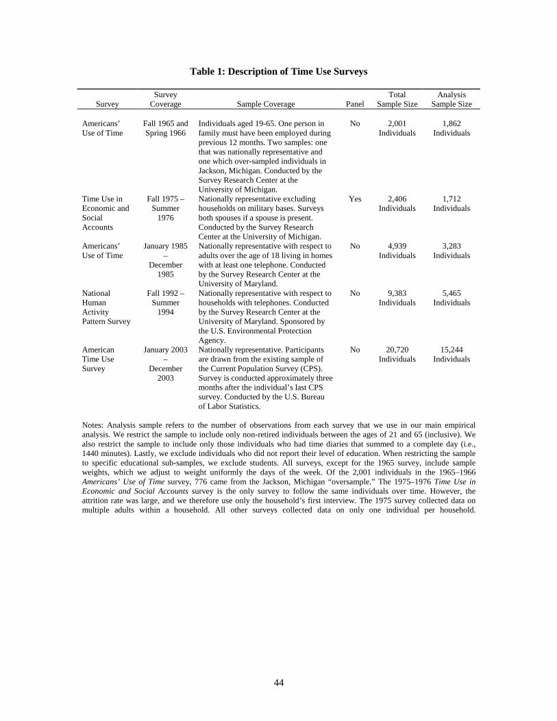
44

Table 1: Description of Time Use Surveys

Survey

Survey Coverage

Sample Coverage

Panel

Total Sample Size

Analysis Sample Size

Americans’ Use of Time

Fall 1965 and Spring 1966

Individuals aged 19-65. One person in family must have been employed during previous 12 months. Two samples: one that was nationally representative and one which over-sampled individuals in Jackson, Michigan. Conducted by the Survey Research Center at the University of Michigan.

No 2,001 Individuals

1,862 Individuals

Time Use in Economic and Social Accounts

Fall 1975 – Summer

1976

Nationally representative excluding households on military bases. Surveys both spouses if a spouse is present. Conducted by the Survey Research Center at the University of Michigan.

Yes 2,406 Individuals

1,712 Individuals

Americans’ Use of Time

January 1985 –

December 1985

Nationally representative with respect to adults over the age of 18 living in homes with at least one telephone. Conducted by the Survey Research Center at the University of Maryland.

No 4,939 Individuals

3,283 Individuals

National Human Activity Pattern Survey

Fall 1992 – Summer

1994

Nationally representative with respect to households with telephones. Conducted by the Survey Research Center at the University of Maryland. Sponsored by the U.S. Environmental Protection Agency.

No 9,383 Individuals

5,465 Individuals

American Time Use Survey

January 2003 –

December 2003

Nationally representative. Participants are drawn from the existing sample of the Current Population Survey (CPS). Survey is conducted approximately three months after the individual’s last CPS survey. Conducted by the U.S. Bureau of Labor Statistics.

No 20,720 Individuals

15,244 Individuals

Notes: Analysis sample refers to the number of observations from each survey that we use in our main empirical analysis. We restrict the sample to include only non-retired individuals between the ages of 21 and 65 (inclusive). We also restrict the sample to include only those individuals who had time diaries that summed to a complete day (i.e., 1440 minutes). Lastly, we exclude individuals who did not report their level of education. When restricting the sample to specific educational sub-samples, we exclude students. All surveys, except for the 1965 survey, include sample weights, which we adjust to weight uniformly the days of the week. Of the 2,001 individuals in the 1965–1966 Americans’ Use of Time survey, 776 came from the Jackson, Michigan “oversample.” The 1975–1976 Time Use in Economic and Social Accounts survey is the only survey to follow the same individuals over time. However, the attrition rate was large, and we therefore use only the household’s first interview. The 1975 survey collected data on multiple adults within a household. All other surveys collected data on only one individual per household.

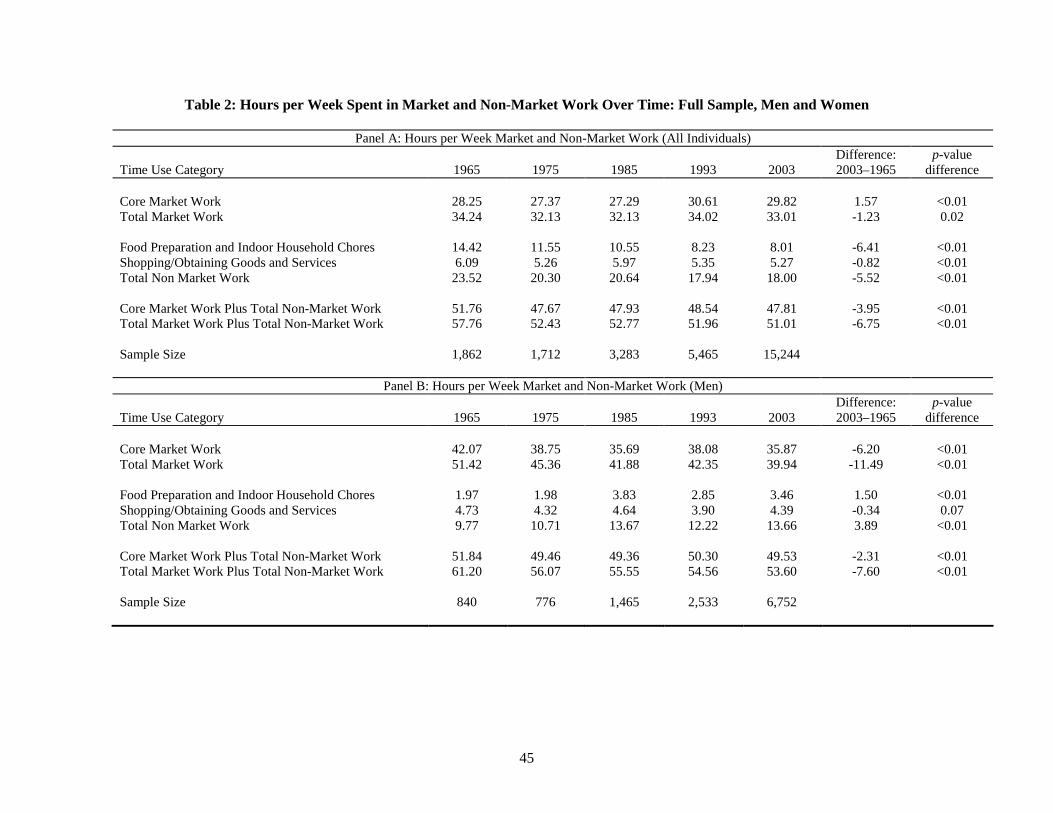
45

Table 2: Hours per Week Spent in Market and Non-Market Work Over Time: Full Sample, Men and Women

Panel A: Hours per Week Market and Non-Market Work (All Individuals) Time Use Category

1965

1975

1985

1993

2003

Difference: 2003–1965

p-value difference

Core Market Work 28.25 27.37 27.29 30.61 29.82 1.57 <0.01 Total Market Work 34.24 32.13 32.13 34.02 33.01 -1.23 0.02 Food Preparation and Indoor Household Chores 14.42 11.55 10.55 8.23 8.01 -6.41 <0.01 Shopping/Obtaining Goods and Services 6.09 5.26 5.97 5.35 5.27 -0.82 <0.01 Total Non Market Work 23.52 20.30 20.64 17.94 18.00 -5.52 <0.01 Core Market Work Plus Total Non-Market Work 51.76 47.67 47.93 48.54 47.81 -3.95 <0.01 Total Market Work Plus Total Non-Market Work 57.76 52.43 52.77 51.96 51.01 -6.75 <0.01 Sample Size 1,862 1,712 3,283 5,465 15,244

Panel B: Hours per Week Market and Non-Market Work (Men) Time Use Category

1965

1975

1985

1993

2003

Difference: 2003–1965

p-value difference

Core Market Work 42.07 38.75 35.69 38.08 35.87 -6.20 <0.01 Total Market Work 51.42 45.36 41.88 42.35 39.94 -11.49 <0.01 Food Preparation and Indoor Household Chores 1.97 1.98 3.83 2.85 3.46 1.50 <0.01 Shopping/Obtaining Goods and Services 4.73 4.32 4.64 3.90 4.39 -0.34 0.07 Total Non Market Work 9.77 10.71 13.67 12.22 13.66 3.89 <0.01 Core Market Work Plus Total Non-Market Work 51.84 49.46 49.36 50.30 49.53 -2.31 <0.01 Total Market Work Plus Total Non-Market Work 61.20 56.07 55.55 54.56 53.60 -7.60 <0.01 Sample Size 840 776 1,465 2,533 6,752

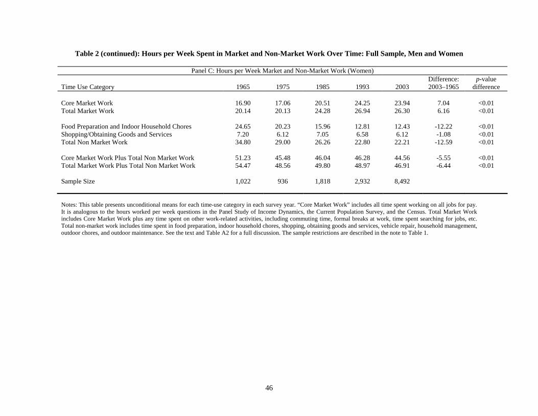
46

Table 2 (continued): Hours per Week Spent in Market and Non-Market Work Over Time: Full Sample, Men and Women

Panel C: Hours per Week Market and Non-Market Work (Women) Time Use Category

1965

1975

1985

1993

2003

Difference: 2003–1965

p-value difference

Core Market Work 16.90 17.06 20.51 24.25 23.94 7.04 <0.01 Total Market Work 20.14 20.13 24.28 26.94 26.30 6.16 <0.01 Food Preparation and Indoor Household Chores 24.65 20.23 15.96 12.81 12.43 -12.22 <0.01 Shopping/Obtaining Goods and Services 7.20 6.12 7.05 6.58 6.12 -1.08 <0.01 Total Non Market Work 34.80 29.00 26.26 22.80 22.21 -12.59 <0.01 Core Market Work Plus Total Non Market Work 51.23 45.48 46.04 46.28 44.56 -5.55 <0.01 Total Market Work Plus Total Non Market Work 54.47 48.56 49.80 48.97 46.91 -6.44 <0.01 Sample Size 1,022 936 1,818 2,932 8,492 Notes: This table presents unconditional means for each time-use category in each survey year. “Core Market Work” includes all time spent working on all jobs for pay. It is analogous to the hours worked per week questions in the Panel Study of Income Dynamics, the Current Population Survey, and the Census. Total Market Work includes Core Market Work plus any time spent on other work-related activities, including commuting time, formal breaks at work, time spent searching for jobs, etc. Total non-market work includes time spent in food preparation, indoor household chores, shopping, obtaining goods and services, vehicle repair, household management, outdoor chores, and outdoor maintenance. See the text and Table A2 for a full discussion. The sample restrictions are described in the note to Table 1.

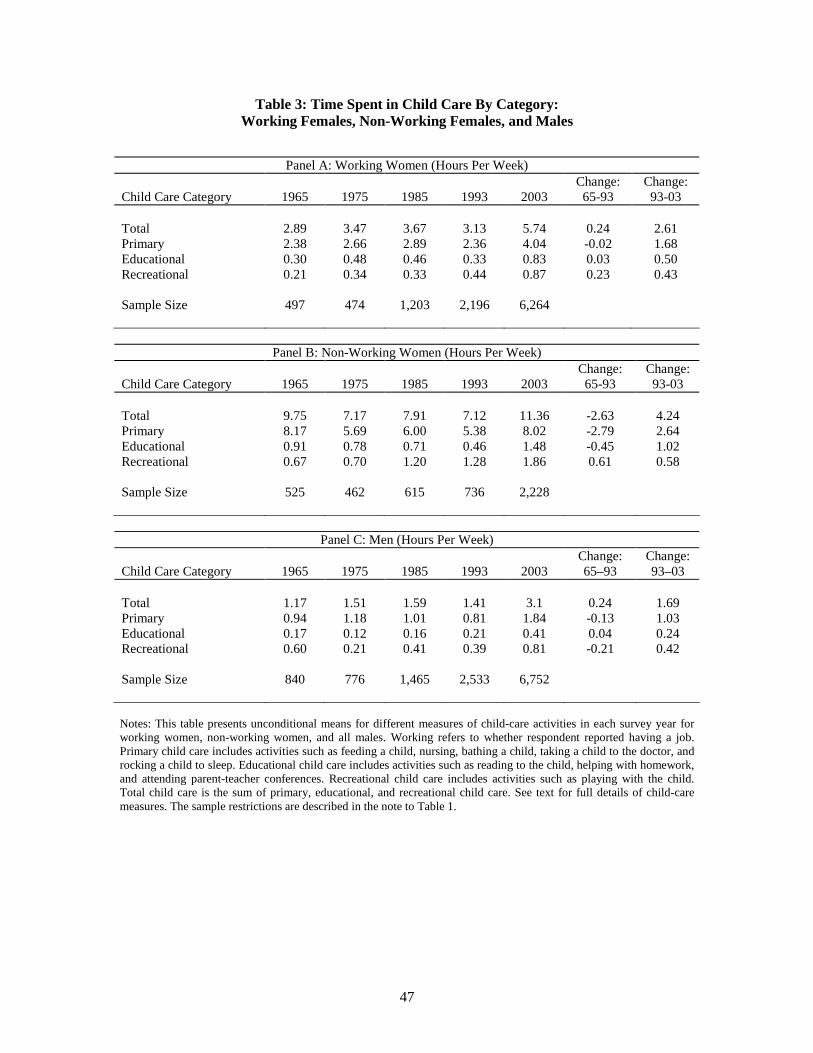
47

Table 3: Time Spent in Child Care By Category: Working Females, Non-Working Females, and Males

Panel A: Working Women (Hours Per Week) Child Care Category

1965

1975

1985

1993

2003

Change: 65-93

Change: 93-03

Total 2.89 3.47 3.67 3.13 5.74 0.24 2.61 Primary 2.38 2.66 2.89 2.36 4.04 -0.02 1.68 Educational 0.30 0.48 0.46 0.33 0.83 0.03 0.50 Recreational 0.21 0.34 0.33 0.44 0.87 0.23 0.43 Sample Size 497 474 1,203 2,196 6,264

Panel B: Non-Working Women (Hours Per Week) Child Care Category

1965

1975

1985

1993

2003

Change: 65-93

Change: 93-03

Total 9.75 7.17 7.91 7.12 11.36 -2.63 4.24 Primary 8.17 5.69 6.00 5.38 8.02 -2.79 2.64 Educational 0.91 0.78 0.71 0.46 1.48 -0.45 1.02 Recreational 0.67 0.70 1.20 1.28 1.86 0.61 0.58 Sample Size 525 462 615 736 2,228

Panel C: Men (Hours Per Week) Child Care Category

1965

1975

1985

1993

2003

Change: 65–93

Change: 93–03

Total 1.17 1.51 1.59 1.41 3.1 0.24 1.69 Primary 0.94 1.18 1.01 0.81 1.84 -0.13 1.03 Educational 0.17 0.12 0.16 0.21 0.41 0.04 0.24 Recreational 0.60 0.21 0.41 0.39 0.81 -0.21 0.42 Sample Size 840 776 1,465 2,533 6,752 Notes: This table presents unconditional means for different measures of child-care activities in each survey year for working women, non-working women, and all males. Working refers to whether respondent reported having a job. Primary child care includes activities such as feeding a child, nursing, bathing a child, taking a child to the doctor, and rocking a child to sleep. Educational child care includes activities such as reading to the child, helping with homework, and attending parent-teacher conferences. Recreational child care includes activities such as playing with the child. Total child care is the sum of primary, educational, and recreational child care. See text for full details of child-care measures. The sample restrictions are described in the note to Table 1.

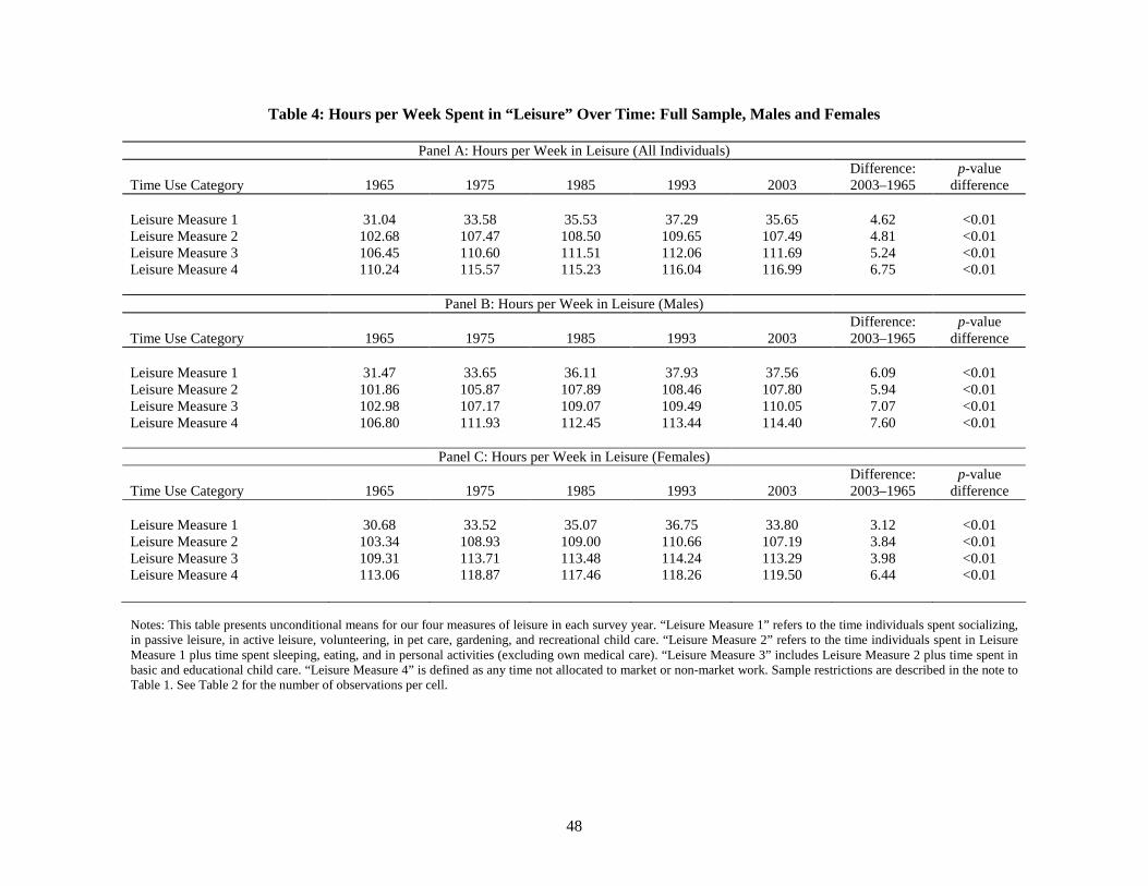
48

Table 4: Hours per Week Spent in “Leisure” Over Time: Full Sample, Males and Females

Panel A: Hours per Week in Leisure (All Individuals) Time Use Category

1965

1975

1985

1993

2003

Difference: 2003–1965

p-value difference

Leisure Measure 1 31.04 33.58 35.53 37.29 35.65 4.62 <0.01 Leisure Measure 2 102.68 107.47 108.50 109.65 107.49 4.81 <0.01 Leisure Measure 3 106.45 110.60 111.51 112.06 111.69 5.24 <0.01 Leisure Measure 4 110.24 115.57 115.23 116.04 116.99 6.75 <0.01

Panel B: Hours per Week in Leisure (Males) Time Use Category

1965

1975

1985

1993

2003

Difference: 2003–1965

p-value difference

Leisure Measure 1 31.47 33.65 36.11 37.93 37.56 6.09 <0.01 Leisure Measure 2 101.86 105.87 107.89 108.46 107.80 5.94 <0.01 Leisure Measure 3 102.98 107.17 109.07 109.49 110.05 7.07 <0.01 Leisure Measure 4 106.80 111.93 112.45 113.44 114.40 7.60 <0.01

Panel C: Hours per Week in Leisure (Females) Time Use Category

1965

1975

1985

1993

2003

Difference: 2003–1965

p-value difference

Leisure Measure 1 30.68 33.52 35.07 36.75 33.80 3.12 <0.01 Leisure Measure 2 103.34 108.93 109.00 110.66 107.19 3.84 <0.01 Leisure Measure 3 109.31 113.71 113.48 114.24 113.29 3.98 <0.01 Leisure Measure 4 113.06 118.87 117.46 118.26 119.50 6.44 <0.01 Notes: This table presents unconditional means for our four measures of leisure in each survey year. “Leisure Measure 1” refers to the time individuals spent socializing, in passive leisure, in active leisure, volunteering, in pet care, gardening, and recreational child care. “Leisure Measure 2” refers to the time individuals spent in Leisure Measure 1 plus time spent sleeping, eating, and in personal activities (excluding own medical care). “Leisure Measure 3” includes Leisure Measure 2 plus time spent in basic and educational child care. “Leisure Measure 4” is defined as any time not allocated to market or non-market work. Sample restrictions are described in the note to Table 1. See Table 2 for the number of observations per cell.

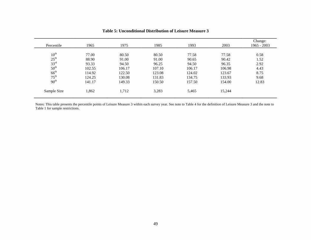
49

Table 5: Unconditional Distribution of Leisure Measure 3

Percentile

1965

1975

1985

1993

2003

Change: 1965 - 2003

10th 77.00 80.50 80.50 77.58 77.58 0.58 25th 88.90 91.00 91.00 90.65 90.42 1.52 33rd 93.33 94.50 96.25 94.50 96.35 2.92 50th 102.55 106.17 107.10 106.17 106.98 4.43 66th 114.92 122.50 123.08 124.02 123.67 8.75 75th 124.25 130.08 131.83 134.75 133.93 9.68 90th 141.17 149.33 150.50 157.50 154.00 12.83

Sample Size 1,862 1,712 3,283 5,465 15,244

Notes: This table presents the percentile points of Leisure Measure 3 within each survey year. See note to Table 4 for the definition of Leisure Measure 3 and the note to Table 1 for sample restrictions.

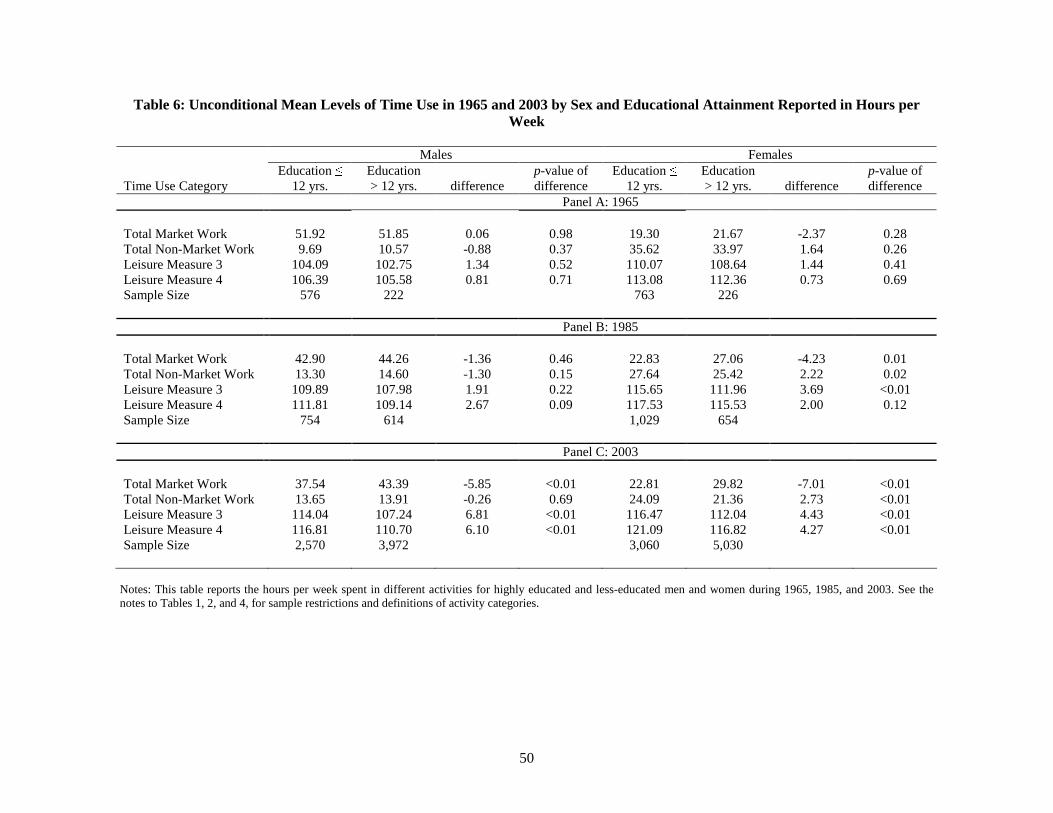
50

Table 6: Unconditional Mean Levels of Time Use in 1965 and 2003 by Sex and Educational Attainment Reported in Hours per Week

Males Females Time Use Category

Education ≤ 12 yrs.

Education > 12 yrs.

difference

p-value of difference

Education ≤ 12 yrs.

Education > 12 yrs.

difference

p-value of difference

Panel A: 1965 Total Market Work 51.92 51.85 0.06 0.98 19.30 21.67 -2.37 0.28 Total Non-Market Work 9.69 10.57 -0.88 0.37 35.62 33.97 1.64 0.26 Leisure Measure 3 104.09 102.75 1.34 0.52 110.07 108.64 1.44 0.41 Leisure Measure 4 106.39 105.58 0.81 0.71 113.08 112.36 0.73 0.69 Sample Size 576 222 763 226

Panel B: 1985 Total Market Work 42.90 44.26 -1.36 0.46 22.83 27.06 -4.23 0.01 Total Non-Market Work 13.30 14.60 -1.30 0.15 27.64 25.42 2.22 0.02 Leisure Measure 3 109.89 107.98 1.91 0.22 115.65 111.96 3.69 <0.01 Leisure Measure 4 111.81 109.14 2.67 0.09 117.53 115.53 2.00 0.12 Sample Size 754 614 1,029 654

Panel C: 2003 Total Market Work 37.54 43.39 -5.85 <0.01 22.81 29.82 -7.01 <0.01 Total Non-Market Work 13.65 13.91 -0.26 0.69 24.09 21.36 2.73 <0.01 Leisure Measure 3 114.04 107.24 6.81 <0.01 116.47 112.04 4.43 <0.01 Leisure Measure 4 116.81 110.70 6.10 <0.01 121.09 116.82 4.27 <0.01 Sample Size 2,570 3,972 3,060 5,030

Notes: This table reports the hours per week spent in different activities for highly educated and less-educated men and women during 1965, 1985, and 2003. See the notes to Tables 1, 2, and 4, for sample restrictions and definitions of activity categories.

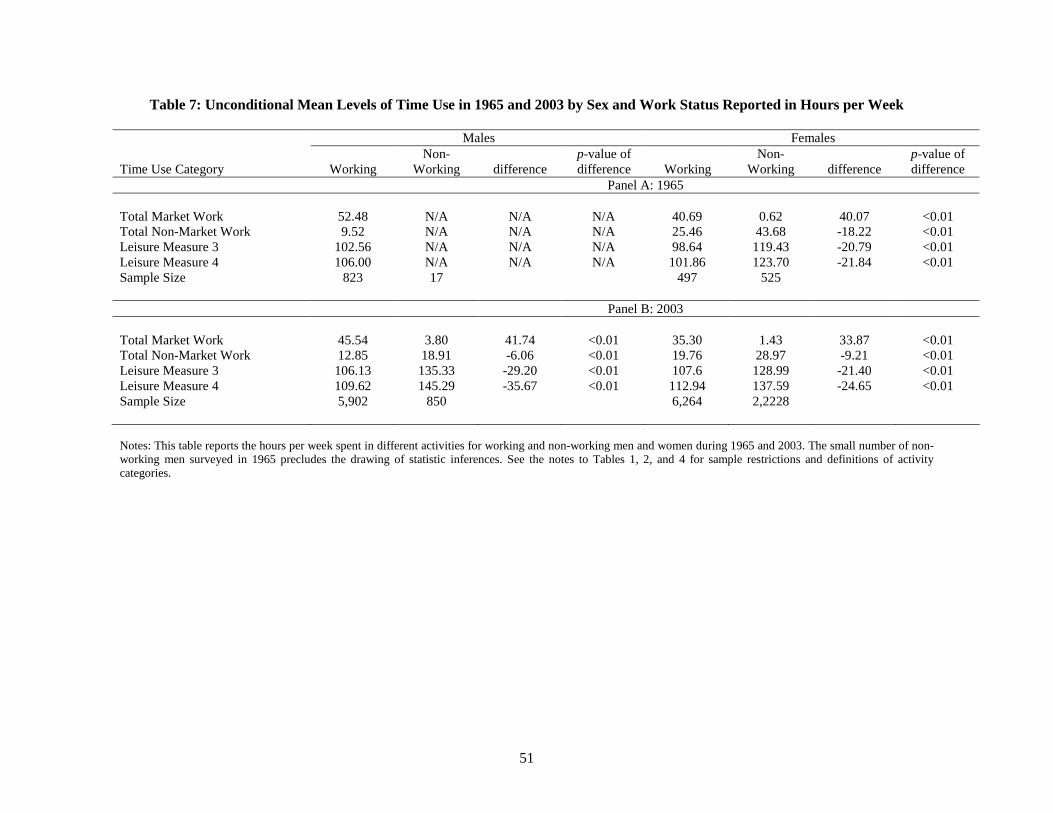
51

Table 7: Unconditional Mean Levels of Time Use in 1965 and 2003 by Sex and Work Status Reported in Hours per Week

Males Females Time Use Category

Working

Non-Working

difference

p-value of difference

Working

Non-Working

difference

p-value of difference

Panel A: 1965 Total Market Work 52.48 N/A N/A N/A 40.69 0.62 40.07 <0.01 Total Non-Market Work 9.52 N/A N/A N/A 25.46 43.68 -18.22 <0.01 Leisure Measure 3 102.56 N/A N/A N/A 98.64 119.43 -20.79 <0.01 Leisure Measure 4 106.00 N/A N/A N/A 101.86 123.70 -21.84 <0.01 Sample Size 823 17 497 525

Panel B: 2003 Total Market Work 45.54 3.80 41.74 <0.01 35.30 1.43 33.87 <0.01 Total Non-Market Work 12.85 18.91 -6.06 <0.01 19.76 28.97 -9.21 <0.01 Leisure Measure 3 106.13 135.33 -29.20 <0.01 107.6 128.99 -21.40 <0.01 Leisure Measure 4 109.62 145.29 -35.67 <0.01 112.94 137.59 -24.65 <0.01 Sample Size 5,902 850 6,264 2,2228 Notes: This table reports the hours per week spent in different activities for working and non-working men and women during 1965 and 2003. The small number of non-working men surveyed in 1965 precludes the drawing of statistic inferences. See the notes to Tables 1, 2, and 4 for sample restrictions and definitions of activity categories.

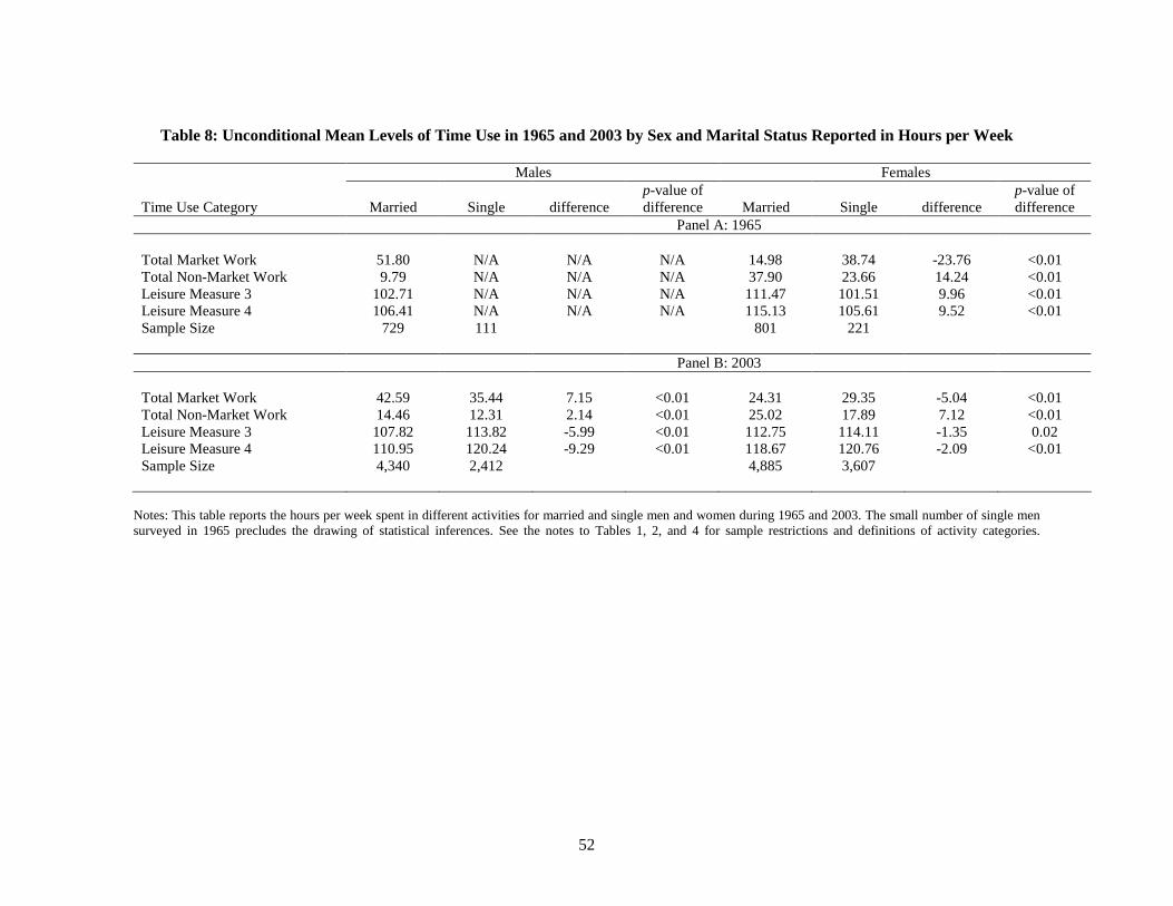
52

Table 8: Unconditional Mean Levels of Time Use in 1965 and 2003 by Sex and Marital Status Reported in Hours per Week

Males Females Time Use Category

Married

Single

difference

p-value of difference

Married

Single

difference

p-value of difference

Panel A: 1965 Total Market Work 51.80 N/A N/A N/A 14.98 38.74 -23.76 <0.01 Total Non-Market Work 9.79 N/A N/A N/A 37.90 23.66 14.24 <0.01 Leisure Measure 3 102.71 N/A N/A N/A 111.47 101.51 9.96 <0.01 Leisure Measure 4 106.41 N/A N/A N/A 115.13 105.61 9.52 <0.01 Sample Size 729 111 801 221

Panel B: 2003 Total Market Work 42.59 35.44 7.15 <0.01 24.31 29.35 -5.04 <0.01 Total Non-Market Work 14.46 12.31 2.14 <0.01 25.02 17.89 7.12 <0.01 Leisure Measure 3 107.82 113.82 -5.99 <0.01 112.75 114.11 -1.35 0.02 Leisure Measure 4 110.95 120.24 -9.29 <0.01 118.67 120.76 -2.09 <0.01 Sample Size 4,340 2,412 4,885 3,607

Notes: This table reports the hours per week spent in different activities for married and single men and women during 1965 and 2003. The small number of single men surveyed in 1965 precludes the drawing of statistical inferences. See the notes to Tables 1, 2, and 4 for sample restrictions and definitions of activity categories.

53

Table 9: Change in Time Use (Relative to 1965) By Sex and Parental Status, Conditional on Demographics (Hours per Week)

Time Use Category

1975

1985

1993

2003

Panel A: Men without Children

Leisure Measure 1 1.12 5.00 7.18 8.01 Leisure Measure 3 4.16 7.32 8.84 9.24 Total Non-Market Work 1.70 3.10 2.48 3.37 Total Market Work -6.48 -9.85 -10.67 -12.98 Sample Size 347 856 2040 3401

Panel B: Men with Children Leisure Measure 1 1.50 3.42 6.01 4.60 Leisure Measure 3 2.75 5.49 6.25 6.84 Total Non-Market Work -0.01 5.00 2.61 4.02 Total Market Work -3.89 -9.19 -8.74 -10.74 Sample Size 429 609 493 3351

Panel C: Women without Children Leisure Measure 1 3.95 6.04 6.94 6.20 Leisure Measure 3 7.75 7.81 8.57 7.69 Total Non-Market Work -1.16 -1.30 -4.47 -6.62 Total Market Work -6.19 -5.63 -3.14 -2.26 Sample Size 377 1012 2175 3666

Panel D: Women with Children Leisure Measure 1 1.82 3.52 6.84 1.65 Leisure Measure 3 1.53 4.18 6.12 4.91 Total Non-Market Work -7.85 -10.28 -13.36 -14.16 Total Market Work 3.99 5.81 7.45 7.13 Sample Size 559 805 757 4826

Notes: This table presents change in time use for men and women with and without children, conditional on demographic changes. Demographic controls include age dummies, education dummies, day-of-week dummies, and a dummy indicating having a child. All changes are reported as hours per week relative to 1965. See the notes to Tables 1, 2, and 4, for sample restrictions and definitions of activity categories.

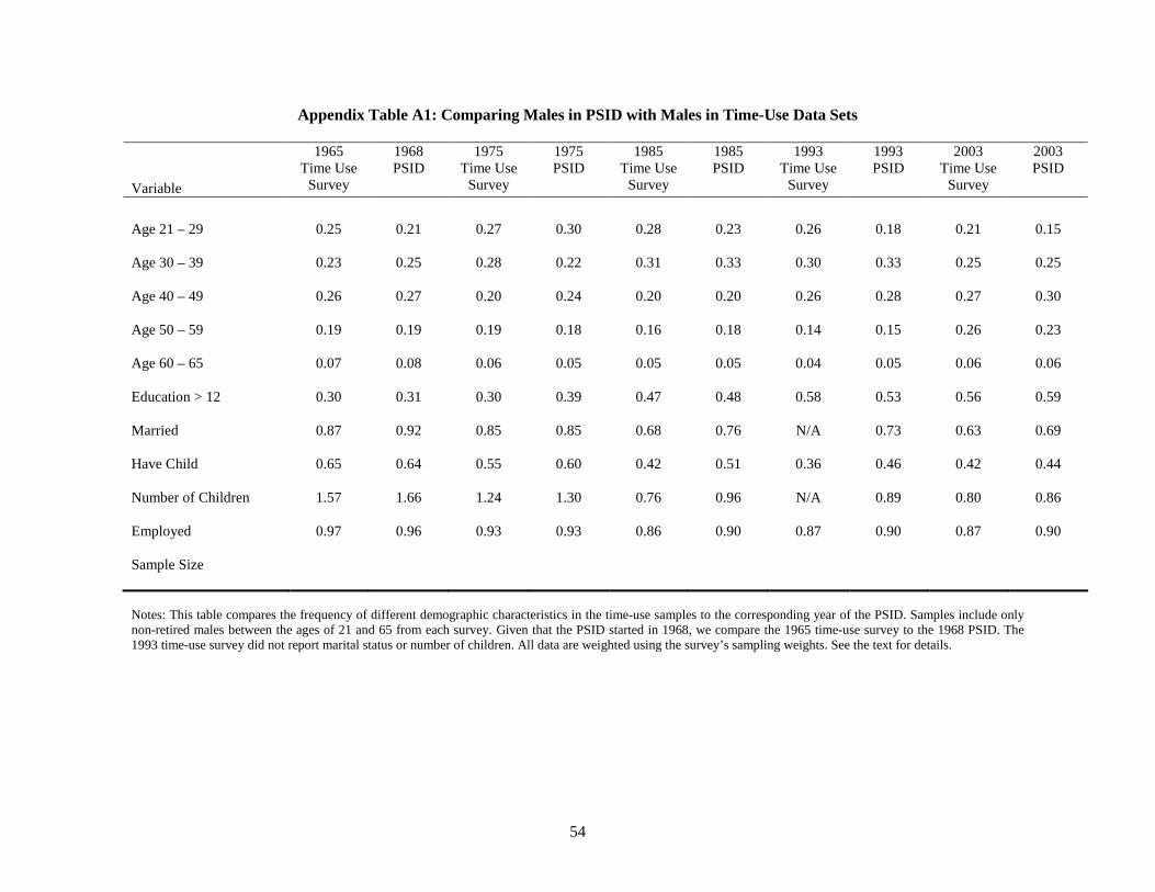
54

Appendix Table A1: Comparing Males in PSID with Males in Time-Use Data Sets

Variable

1965 Time Use Survey

1968 PSID

1975 Time Use Survey

1975 PSID

1985 Time Use Survey

1985 PSID

1993 Time Use Survey

1993 PSID

2003 Time Use Survey

2003 PSID

Age 21 – 29

0.25 0.21 0.27 0.30 0.28 0.23 0.26 0.18 0.21 0.15

Age 30 – 39

0.23 0.25 0.28 0.22 0.31 0.33 0.30 0.33 0.25 0.25

Age 40 – 49

0.26 0.27 0.20 0.24 0.20 0.20 0.26 0.28 0.27 0.30

Age 50 – 59

0.19 0.19 0.19 0.18 0.16 0.18 0.14 0.15 0.26 0.23

Age 60 – 65

0.07 0.08 0.06 0.05 0.05 0.05 0.04 0.05 0.06 0.06

Education > 12

0.30 0.31 0.30 0.39 0.47 0.48 0.58 0.53 0.56 0.59

Married

0.87 0.92 0.85 0.85 0.68 0.76 N/A 0.73 0.63 0.69

Have Child

0.65 0.64 0.55 0.60 0.42 0.51 0.36 0.46 0.42 0.44

Number of Children

1.57 1.66 1.24 1.30 0.76 0.96 N/A 0.89 0.80 0.86

Employed

0.97 0.96 0.93 0.93 0.86 0.90 0.87 0.90 0.87 0.90

Sample Size

Notes: This table compares the frequency of different demographic characteristics in the time-use samples to the corresponding year of the PSID. Samples include only non-retired males between the ages of 21 and 65 from each survey. Given that the PSID started in 1968, we compare the 1965 time-use survey to the 1968 PSID. The 1993 time-use survey did not report marital status or number of children. All data are weighted using the survey’s sampling weights. See the text for details.

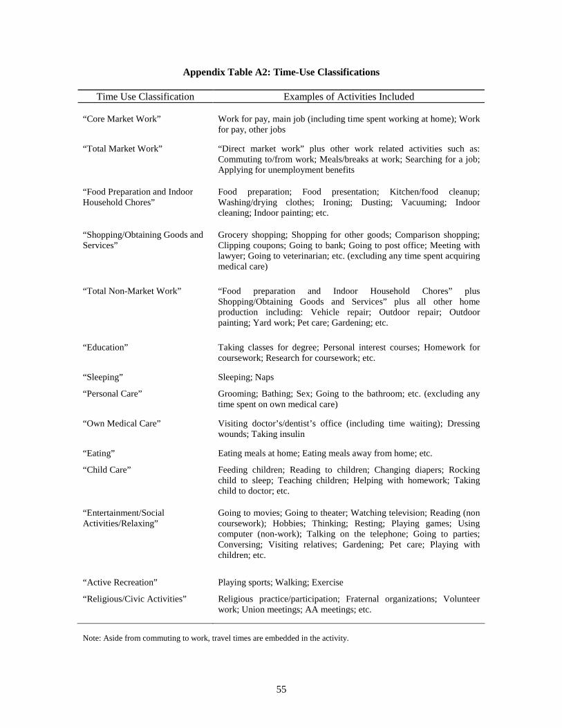
55

Appendix Table A2: Time-Use Classifications

Time Use Classification Examples of Activities Included “Core Market Work” Work for pay, main job (including time spent working at home); Work

for pay, other jobs

“Total Market Work” “Direct market work” plus other work related activities such as: Commuting to/from work; Meals/breaks at work; Searching for a job; Applying for unemployment benefits

“Food Preparation and Indoor Household Chores”

Food preparation; Food presentation; Kitchen/food cleanup; Washing/drying clothes; Ironing; Dusting; Vacuuming; Indoor cleaning; Indoor painting; etc.

“Shopping/Obtaining Goods and Services”

Grocery shopping; Shopping for other goods; Comparison shopping; Clipping coupons; Going to bank; Going to post office; Meeting with lawyer; Going to veterinarian; etc. (excluding any time spent acquiring medical care)

“Total Non-Market Work” “Food preparation and Indoor Household Chores” plus Shopping/Obtaining Goods and Services” plus all other home production including: Vehicle repair; Outdoor repair; Outdoor painting; Yard work; Pet care; Gardening; etc.

“Education” Taking classes for degree; Personal interest courses; Homework for coursework; Research for coursework; etc.

“Sleeping” Sleeping; Naps

“Personal Care” Grooming; Bathing; Sex; Going to the bathroom; etc. (excluding any time spent on own medical care)

“Own Medical Care” Visiting doctor’s/dentist’s office (including time waiting); Dressing wounds; Taking insulin

“Eating” Eating meals at home; Eating meals away from home; etc.

“Child Care” Feeding children; Reading to children; Changing diapers; Rocking child to sleep; Teaching children; Helping with homework; Taking child to doctor; etc.

“Entertainment/Social Activities/Relaxing”

Going to movies; Going to theater; Watching television; Reading (non coursework); Hobbies; Thinking; Resting; Playing games; Using computer (non-work); Talking on the telephone; Going to parties; Conversing; Visiting relatives; Gardening; Pet care; Playing with children; etc.

“Active Recreation” Playing sports; Walking; Exercise

“Religious/Civic Activities” Religious practice/participation; Fraternal organizations; Volunteer work; Union meetings; AA meetings; etc.

Note: Aside from commuting to work, travel times are embedded in the activity.

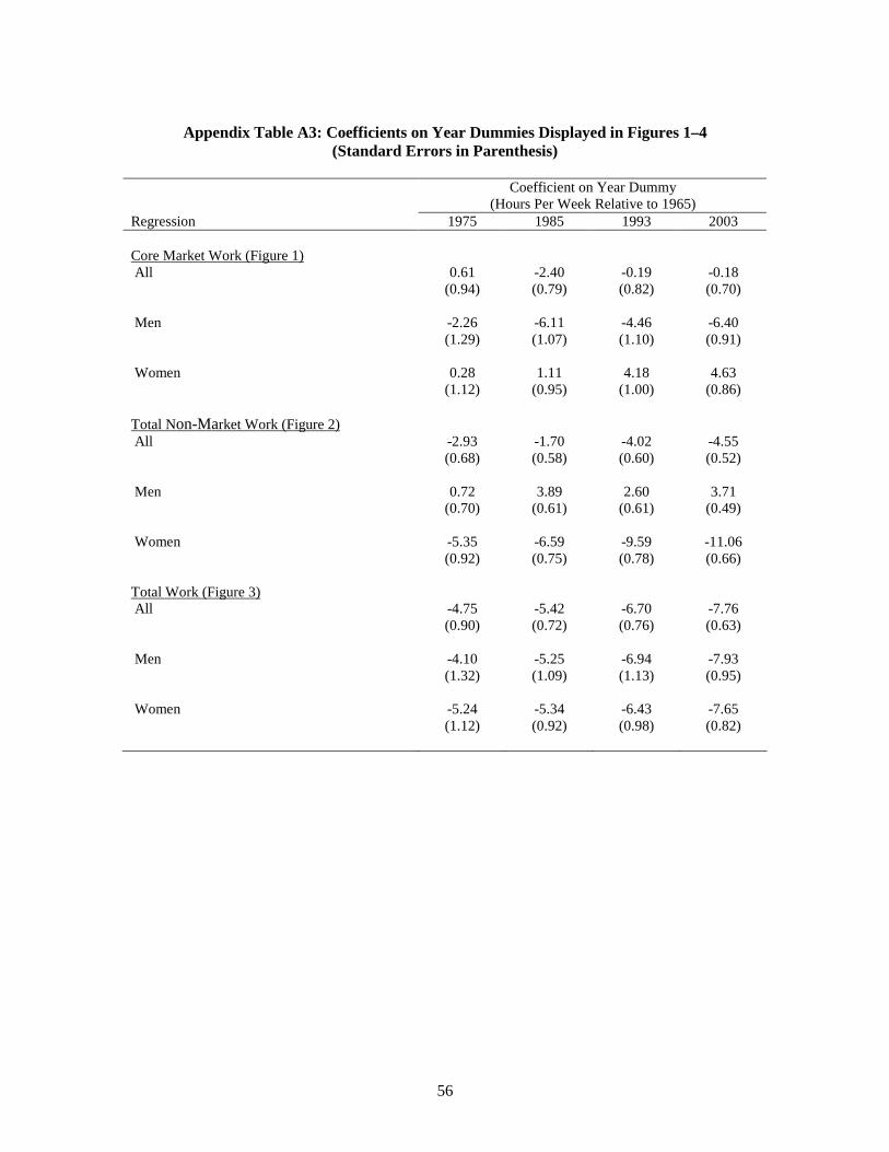
56

Appendix Table A3: Coefficients on Year Dummies Displayed in Figures 1–4

(Standard Errors in Parenthesis) Coefficient on Year Dummy

(Hours Per Week Relative to 1965) Regression 1975 1985 1993 2003 Core Market Work (Figure 1) All 0.61 -2.40 -0.19 -0.18 (0.94) (0.79) (0.82) (0.70) Men -2.26 -6.11 -4.46 -6.40 (1.29) (1.07) (1.10) (0.91) Women 0.28 1.11 4.18 4.63 (1.12) (0.95) (1.00) (0.86) Total Non-Market Work (Figure 2) All -2.93 -1.70 -4.02 -4.55 (0.68) (0.58) (0.60) (0.52) Men 0.72 3.89 2.60 3.71 (0.70) (0.61) (0.61) (0.49) Women -5.35 -6.59 -9.59 -11.06 (0.92) (0.75) (0.78) (0.66) Total Work (Figure 3) All -4.75 -5.42 -6.70 -7.76 (0.90) (0.72) (0.76) (0.63) Men -4.10 -5.25 -6.94 -7.93 (1.32) (1.09) (1.13) (0.95) Women -5.24 -5.34 -6.43 -7.65 (1.12) (0.92) (0.98) (0.82)

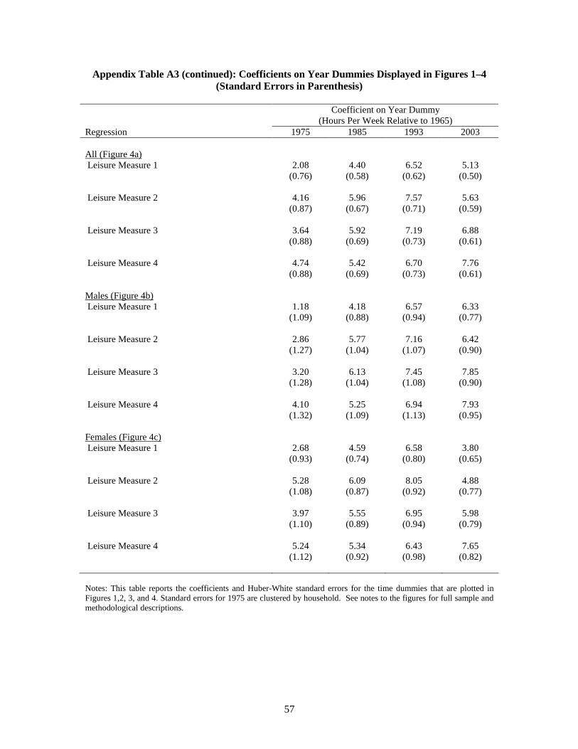
57

Appendix Table A3 (continued): Coefficients on Year Dummies Displayed in Figures 1–4 (Standard Errors in Parenthesis)

Coefficient on Year Dummy

(Hours Per Week Relative to 1965) Regression 1975 1985 1993 2003 All (Figure 4a) Leisure Measure 1 2.08 4.40 6.52 5.13 (0.76) (0.58) (0.62) (0.50) Leisure Measure 2 4.16 5.96 7.57 5.63 (0.87) (0.67) (0.71) (0.59) Leisure Measure 3 3.64 5.92 7.19 6.88 (0.88) (0.69) (0.73) (0.61) Leisure Measure 4 4.74 5.42 6.70 7.76 (0.88) (0.69) (0.73) (0.61) Males (Figure 4b) Leisure Measure 1 1.18 4.18 6.57 6.33 (1.09) (0.88) (0.94) (0.77) Leisure Measure 2 2.86 5.77 7.16 6.42 (1.27) (1.04) (1.07) (0.90) Leisure Measure 3 3.20 6.13 7.45 7.85 (1.28) (1.04) (1.08) (0.90) Leisure Measure 4 4.10 5.25 6.94 7.93 (1.32) (1.09) (1.13) (0.95) Females (Figure 4c) Leisure Measure 1 2.68 4.59 6.58 3.80 (0.93) (0.74) (0.80) (0.65) Leisure Measure 2 5.28 6.09 8.05 4.88 (1.08) (0.87) (0.92) (0.77) Leisure Measure 3 3.97 5.55 6.95 5.98 (1.10) (0.89) (0.94) (0.79) Leisure Measure 4 5.24 5.34 6.43 7.65 (1.12) (0.92) (0.98) (0.82) Notes: This table reports the coefficients and Huber-White standard errors for the time dummies that are plotted in Figures 1,2, 3, and 4. Standard errors for 1975 are clustered by household. See notes to the figures for full sample and methodological descriptions.

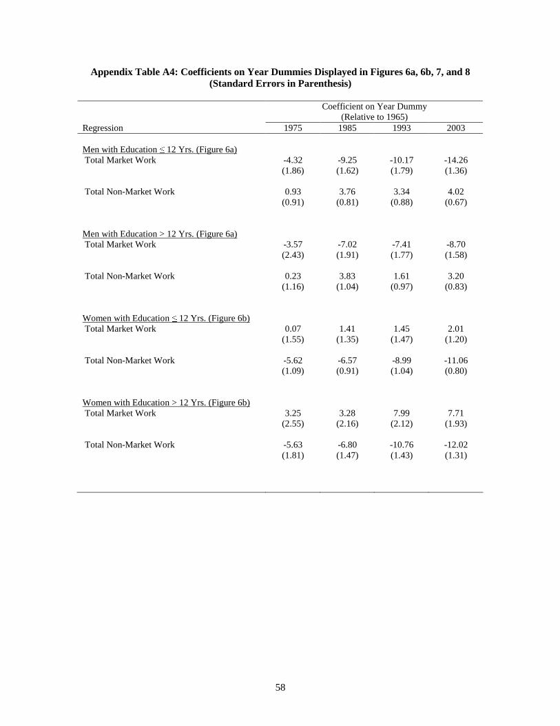
58

Appendix Table A4: Coefficients on Year Dummies Displayed in Figures 6a, 6b, 7, and 8 (Standard Errors in Parenthesis)

Coefficient on Year Dummy

(Relative to 1965) Regression 1975 1985 1993 2003 Men with Education ≤ 12 Yrs. (Figure 6a) Total Market Work -4.32 -9.25 -10.17 -14.26 (1.86) (1.62) (1.79) (1.36) Total Non-Market Work 0.93 3.76 3.34 4.02 (0.91) (0.81) (0.88) (0.67) Men with Education > 12 Yrs. (Figure 6a) Total Market Work -3.57 -7.02 -7.41 -8.70 (2.43) (1.91) (1.77) (1.58) Total Non-Market Work 0.23 3.83 1.61 3.20 (1.16) (1.04) (0.97) (0.83) Women with Education ≤ 12 Yrs. (Figure 6b) Total Market Work 0.07 1.41 1.45 2.01 (1.55) (1.35) (1.47) (1.20) Total Non-Market Work -5.62 -6.57 -8.99 -11.06 (1.09) (0.91) (1.04) (0.80) Women with Education > 12 Yrs. (Figure 6b) Total Market Work 3.25 3.28 7.99 7.71 (2.55) (2.16) (2.12) (1.93) Total Non-Market Work -5.63 -6.80 -10.76 -12.02 (1.81) (1.47) (1.43) (1.31)

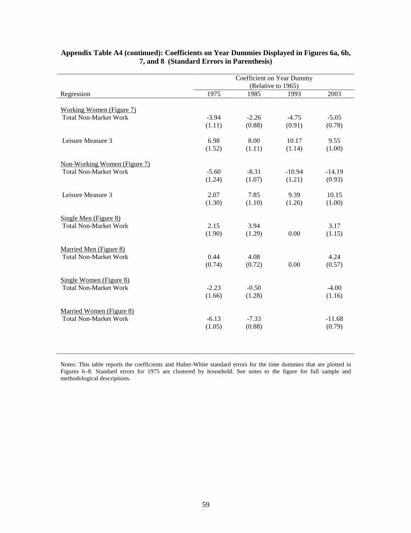
59

Appendix Table A4 (continued): Coefficients on Year Dummies Displayed in Figures 6a, 6b, 7, and 8 (Standard Errors in Parenthesis)

Coefficient on Year Dummy

(Relative to 1965) Regression 1975 1985 1993 2003 Working Women (Figure 7) Total Non-Market Work -3.94 -2.26 -4.75 -5.05 (1.11) (0.88) (0.91) (0.78) Leisure Measure 3 6.98 8.00 10.17 9.55 (1.52) (1.11) (1.14) (1.00) Non-Working Women (Figure 7) Total Non-Market Work -5.60 -8.31 -10.94 -14.19 (1.24) (1.07) (1.21) (0.93) Leisure Measure 3 2.07 7.85 9.39 10.15 (1.30) (1.10) (1.26) (1.00) Single Men (Figure 8) Total Non-Market Work 2.15 3.94 3.17 (1.90) (1.29) 0.00 (1.15) Married Men (Figure 8) Total Non-Market Work 0.44 4.08 4.24 (0.74) (0.72) 0.00 (0.57) Single Women (Figure 8) Total Non-Market Work -2.23 -0.50 -4.00 (1.66) (1.28) (1.16) Married Women (Figure 8) Total Non-Market Work -6.13 -7.33 -11.68 (1.05) (0.88) (0.79) Notes: This table reports the coefficients and Huber-White standard errors for the time dummies that are plotted in Figures 6–8. Standard errors for 1975 are clustered by household. See notes to the figure for full sample and methodological descriptions.

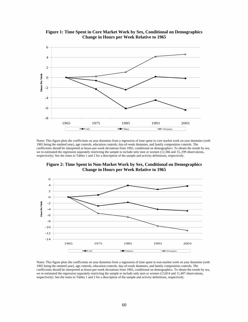
60

Figure 1: Time Spent in Core Market Work by Sex, Conditional on Demographics Change in Hours per Week Relative to 1965

-8

-6

-4

-2

0

2

4

6

1965 1975 1985 1993 2003

Hour

s P

er W

eek

All Men Women

Notes: This figure plots the coefficients on year dummies from a regression of time spent in core market work on year dummies (with 1965 being the omitted year), age controls, education controls, day-of-week dummies, and family composition controls. The coefficients should be interpreted as hours-per-week deviations from 1965, conditional on demographics. To obtain the trends by sex, we re-estimated the regression separately restricting the sample to include only men or women (12,366 and 15,,199 observations, respectively). See the notes to Tables 1 and 2 for a description of the sample and activity definitions, respectively.

Figure 2: Time Spent in Non-Market Work by Sex, Conditional on Demographics Change in Hours per Week Relative to 1965

-14

-12

-10

-8

-6

-4

-2

0

2

4

6

1965 1975 1985 1993 2003

Hou

rs P

er W

eek

All Males Females

Notes: This figure plots the coefficients on year dummies from a regression of time spent in non-market work on year dummies (with 1965 being the omitted year), age controls, education controls, day-of-week dummies, and family composition controls. The coefficients should be interpreted as hours-per-week deviations from 1965, conditional on demographics. To obtain the trends by sex, we re-estimated the regression separately restricting the sample to include only men or women (13,814 and 11,407 observations, respectively). See the notes to Tables 1 and 2 for a description of the sample and activity definitions, respectively.

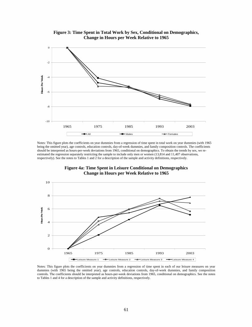
61

Figure 3: Time Spent in Total Work by Sex, Conditional on Demographics, Change in Hours per Week Relative to 1965

-10

-8

-6

-4

-2

0

1965 1975 1985 1993 2003

Hou

rs P

er W

eek

All Males Females

Notes: This figure plots the coefficients on year dummies from a regression of time spent in total work on year dummies (with 1965 being the omitted year), age controls, education controls, day-of-week dummies, and family composition controls. The coefficients should be interpreted as hours-per-week deviations from 1965, conditional on demographics. To obtain the trends by sex, we re-estimated the regression separately restricting the sample to include only men or women (13,814 and 11,407 observations, respectively). See the notes to Tables 1 and 2 for a description of the sample and activity definitions, respectively.

Figure 4a: Time Spent in Leisure Conditional on Demographics

Change in Hours per Week Relative to 1965

0

2

4

6

8

10

1965 1975 1985 1993 2003

Hou

rs P

er W

eek

Leisure Measure 1 Leisure Measure 2 Leisure Measure 3 Leisure Measure 4

Notes: This figure plots the coefficients on year dummies from a regression of time spent in each of our leisure measures on year dummies (with 1965 being the omitted year), age controls, education controls, day-of-week dummies, and family composition controls. The coefficients should be interpreted as hours-per-week deviations from 1965, conditional on demographics. See the notes to Tables 1 and 4 for a description of the sample and activity definitions, respectively.

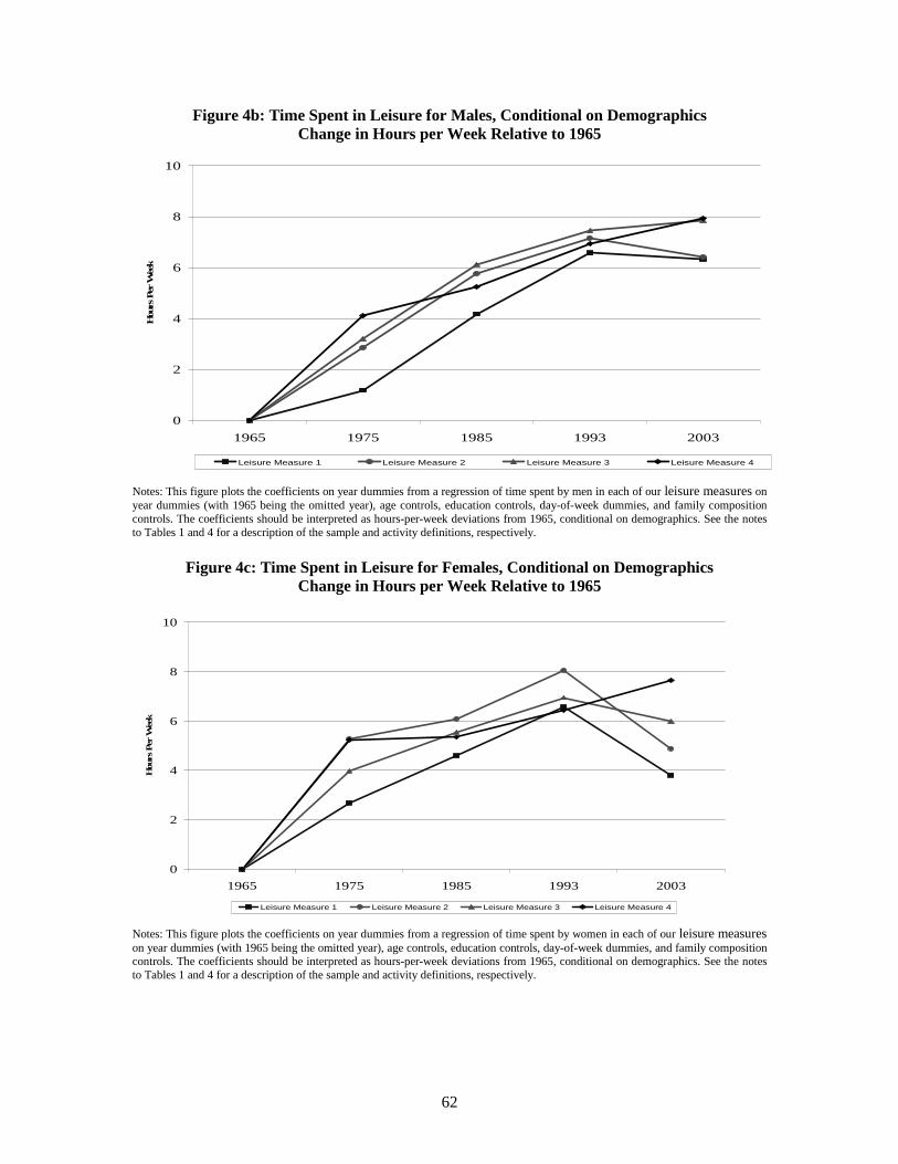
62

Figure 4b: Time Spent in Leisure for Males, Conditional on Demographics Change in Hours per Week Relative to 1965

0

2

4

6

8

10

1965 1975 1985 1993 2003

Hou

rs P

er W

eek

Leisure Measure 1 Leisure Measure 2 Leisure Measure 3 Leisure Measure 4

Notes: This figure plots the coefficients on year dummies from a regression of time spent by men in each of our leisure measures on year dummies (with 1965 being the omitted year), age controls, education controls, day-of-week dummies, and family composition controls. The coefficients should be interpreted as hours-per-week deviations from 1965, conditional on demographics. See the notes to Tables 1 and 4 for a description of the sample and activity definitions, respectively.

Figure 4c: Time Spent in Leisure for Females, Conditional on Demographics

Change in Hours per Week Relative to 1965

0

2

4

6

8

10

1965 1975 1985 1993 2003

Hou

rs P

er W

eek

Leisure Measure 1 Leisure Measure 2 Leisure Measure 3 Leisure Measure 4

Notes: This figure plots the coefficients on year dummies from a regression of time spent by women in each of our leisure measures on year dummies (with 1965 being the omitted year), age controls, education controls, day-of-week dummies, and family composition controls. The coefficients should be interpreted as hours-per-week deviations from 1965, conditional on demographics. See the notes to Tables 1 and 4 for a description of the sample and activity definitions, respectively.

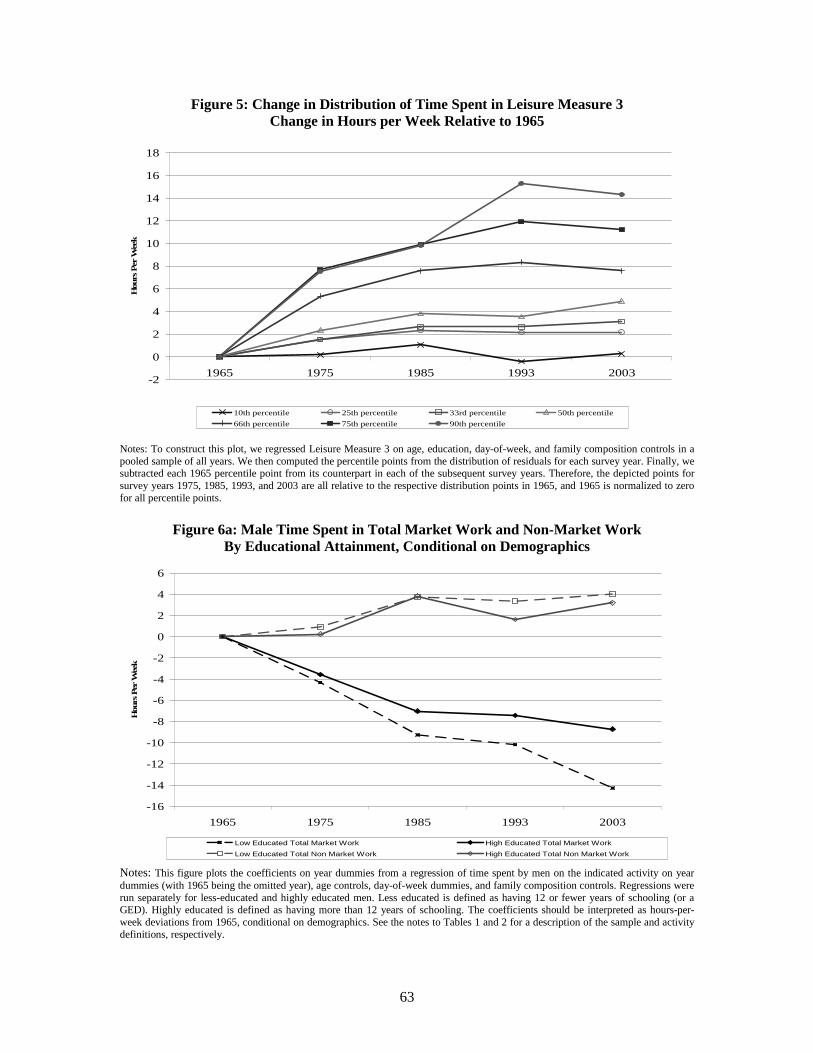
63

Figure 5: Change in Distribution of Time Spent in Leisure Measure 3 Change in Hours per Week Relative to 1965

-2

0

2

4

6

8

10

12

14

16

18

1965 1975 1985 1993 2003

Hour

s Per W

eek

10th percentile 25th percentile 33rd percentile 50th percentile

66th percentile 75th percentile 90th percentile

Notes: To construct this plot, we regressed Leisure Measure 3 on age, education, day-of-week, and family composition controls in a pooled sample of all years. We then computed the percentile points from the distribution of residuals for each survey year. Finally, we subtracted each 1965 percentile point from its counterpart in each of the subsequent survey years. Therefore, the depicted points for survey years 1975, 1985, 1993, and 2003 are all relative to the respective distribution points in 1965, and 1965 is normalized to zero for all percentile points.

Figure 6a: Male Time Spent in Total Market Work and Non-Market Work

By Educational Attainment, Conditional on Demographics

-16

-14

-12

-10

-8

-6

-4

-2

0

2

4

6

1965 1975 1985 1993 2003

Hour

s Per W

eek

Low Educated Total Market Work High Educated Total Market Work

Low Educated Total Non Market Work High Educated Total Non Market Work

Notes: This figure plots the coefficients on year dummies from a regression of time spent by men on the indicated activity on year dummies (with 1965 being the omitted year), age controls, day-of-week dummies, and family composition controls. Regressions were run separately for less-educated and highly educated men. Less educated is defined as having 12 or fewer years of schooling (or a GED). Highly educated is defined as having more than 12 years of schooling. The coefficients should be interpreted as hours-per-week deviations from 1965, conditional on demographics. See the notes to Tables 1 and 2 for a description of the sample and activity definitions, respectively.

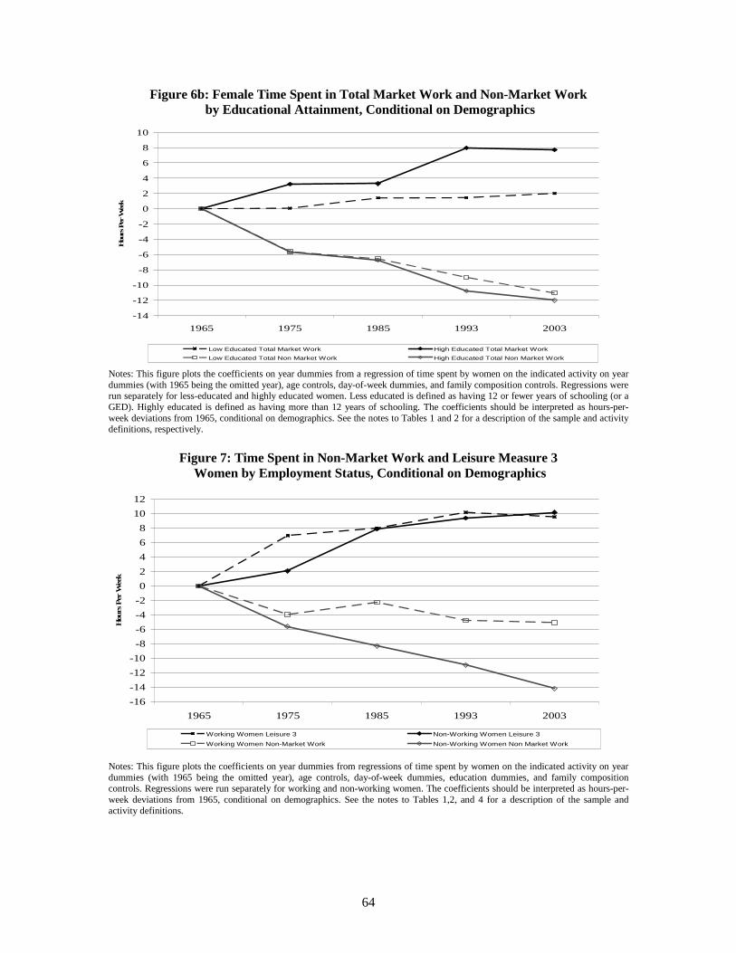
64

Figure 6b: Female Time Spent in Total Market Work and Non-Market Work by Educational Attainment, Conditional on Demographics

-14

-12

-10

-8

-6

-4

-2

0

2

4

6

8

10

1965 1975 1985 1993 2003

Hou

rs P

er W

eek

Low Educated Total Market Work High Educated Total Market Work

Low Educated Total Non Market Work High Educated Total Non Market Work

Notes: This figure plots the coefficients on year dummies from a regression of time spent by women on the indicated activity on year dummies (with 1965 being the omitted year), age controls, day-of-week dummies, and family composition controls. Regressions were run separately for less-educated and highly educated women. Less educated is defined as having 12 or fewer years of schooling (or a GED). Highly educated is defined as having more than 12 years of schooling. The coefficients should be interpreted as hours-per-week deviations from 1965, conditional on demographics. See the notes to Tables 1 and 2 for a description of the sample and activity definitions, respectively.

Figure 7: Time Spent in Non-Market Work and Leisure Measure 3

Women by Employment Status, Conditional on Demographics

-16

-14

-12

-10

-8

-6

-4

-2

0

2

4

6

8

10

12

1965 1975 1985 1993 2003

Hou

rs P

er W

eek

Working Women Leisure 3 Non-Working Women Leisure 3

Working Women Non-Market Work Non-Working Women Non Market Work

Notes: This figure plots the coefficients on year dummies from regressions of time spent by women on the indicated activity on year dummies (with 1965 being the omitted year), age controls, day-of-week dummies, education dummies, and family composition controls. Regressions were run separately for working and non-working women. The coefficients should be interpreted as hours-per-week deviations from 1965, conditional on demographics. See the notes to Tables 1,2, and 4 for a description of the sample and activity definitions.

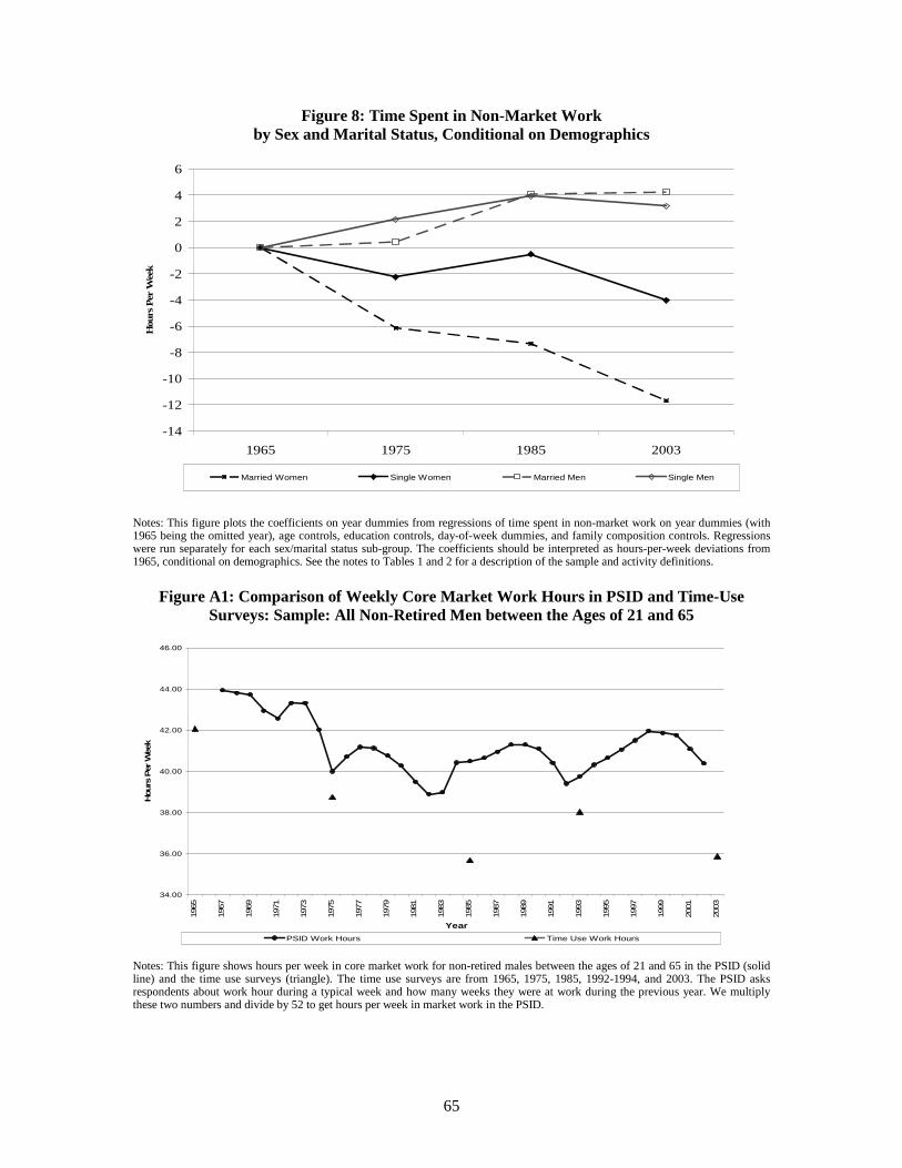
65

Figure 8: Time Spent in Non-Market Work by Sex and Marital Status, Conditional on Demographics

-14

-12

-10

-8

-6

-4

-2

0

2

4

6

1965 1975 1985 2003

Hou

rs P

er W

eek

Married Women Single Women Married Men Single Men

Notes: This figure plots the coefficients on year dummies from regressions of time spent in non-market work on year dummies (with 1965 being the omitted year), age controls, education controls, day-of-week dummies, and family composition controls. Regressions were run separately for each sex/marital status sub-group. The coefficients should be interpreted as hours-per-week deviations from 1965, conditional on demographics. See the notes to Tables 1 and 2 for a description of the sample and activity definitions.

Figure A1: Comparison of Weekly Core Market Work Hours in PSID and Time-Use

Surveys: Sample: All Non-Retired Men between the Ages of 21 and 65

34.00

36.00

38.00

40.00

42.00

44.00

46.00

1965

1967

1969

1971

1973

1975

1977

1979

1981

1983

1985

1987

1989

1991

1993

1995

1997

1999

2001

2003

Year

Hours

Per

Wee

k

PSID Work Hours Time Use Work Hours

Notes: This figure shows hours per week in core market work for non-retired males between the ages of 21 and 65 in the PSID (solid line) and the time use surveys (triangle). The time use surveys are from 1965, 1975, 1985, 1992-1994, and 2003. The PSID asks respondents about work hour during a typical week and how many weeks they were at work during the previous year. We multiply these two numbers and divide by 52 to get hours per week in market work in the PSID.