Measuring the Dynamic Response of a Structure

• This week in lab– Experiment 6 – application of the analogue instrumentation you

met in the 1st Instrumentation Lab period.– Works just like a regular experiment

• Read manual• Meet with your team in advance• Visit the lab• Do a logbook preparation• Logbook is graded

– Note your logbook preparation should be submitted to Dustin Grissom (dgrissom@vt.edu) not your regular TA.

• Next class 3/12 (no class next week)– Making measurements with computers– Read the ‘Digital Measurements’ section of the manual

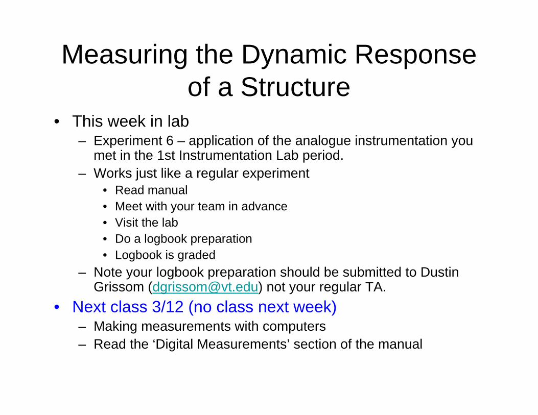
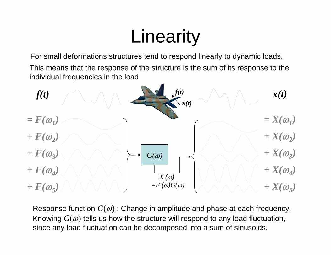
Dynamic Response of a Structure

• Characterizing how a structure will respond to a time-varying set of loads is a fundamental requirement of engineering in aero, ocean and space applications

f(t)

= F(ω1)

+ F(ω2)

+ F(ω3)

+ F(ω4)

+ F(ω5)

x(t)

= X(ω1)

+ X(ω2)

+ X(ω3)

+ X(ω4)

+ X(ω5)

G(ω)

X (ω)=F (ω)G(ω)

f(t)

x(t)

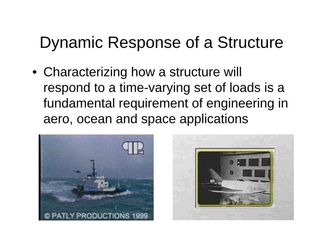
LinearityFor small deformations structures tend to respond linearly to dynamic loads.This means that the response of the structure is the sum of its response to the individual frequencies in the load

Response function G(ω) : Change in amplitude and phase at each frequency.Knowing G(ω) tells us how the structure will respond to any load fluctuation, since any load fluctuation can be decomposed into a sum of sinusoids.

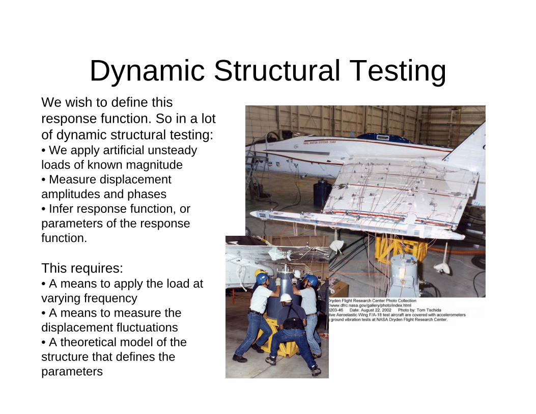
Dynamic Structural TestingWe wish to define this response function. So in a lot of dynamic structural testing: • We apply artificial unsteady loads of known magnitude• Measure displacement amplitudes and phases• Infer response function, or parameters of the response function.

This requires:• A means to apply the load at varying frequency• A means to measure the displacement fluctuations• A theoretical model of the structure that defines the parameters

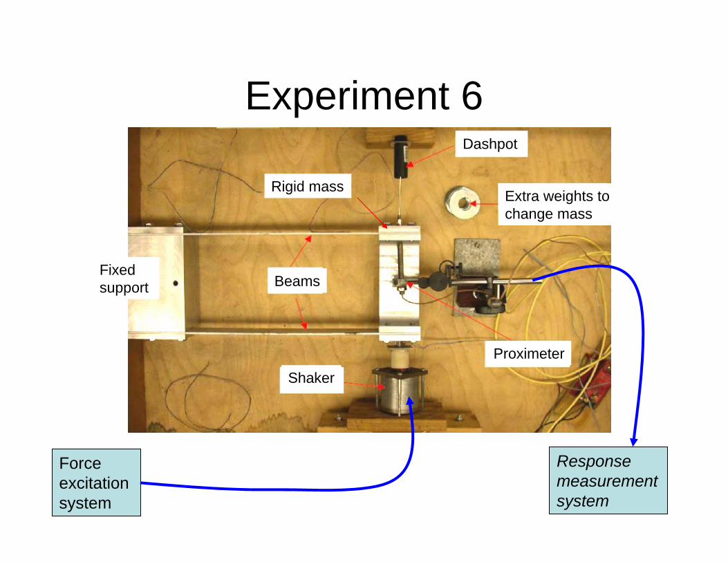
Experiment 6

Force excitationsystem

Response measurement system

Beams

ShakerProximeter

Extra weights to change mass

Dashpot

Fixed support

Rigid mass

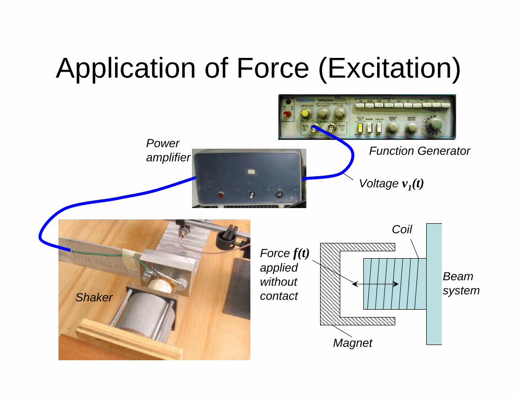
Application of Force (Excitation)

Magnet

Coil

Beam system

Function GeneratorPower amplifier

Force f(t)applied without contact

Voltage v1(t)

Shaker

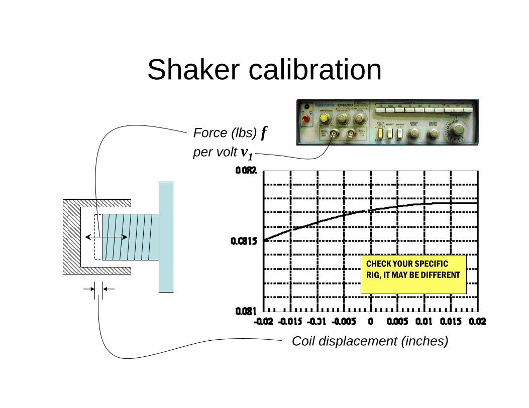
Shaker calibration

Force (lbs) f per volt v1

Coil displacement (inches)

CHECK YOUR SPECIFIC RIG, IT MAY BE DIFFERENT

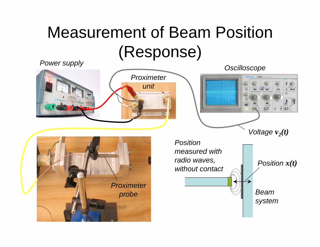
Measurement of Beam Position (Response)

Beam system

Voltage v2(t)

Position x(t)

Position measured with radio waves, without contact

Power supplyOscilloscope

Proximeterunit

Proximeterprobe

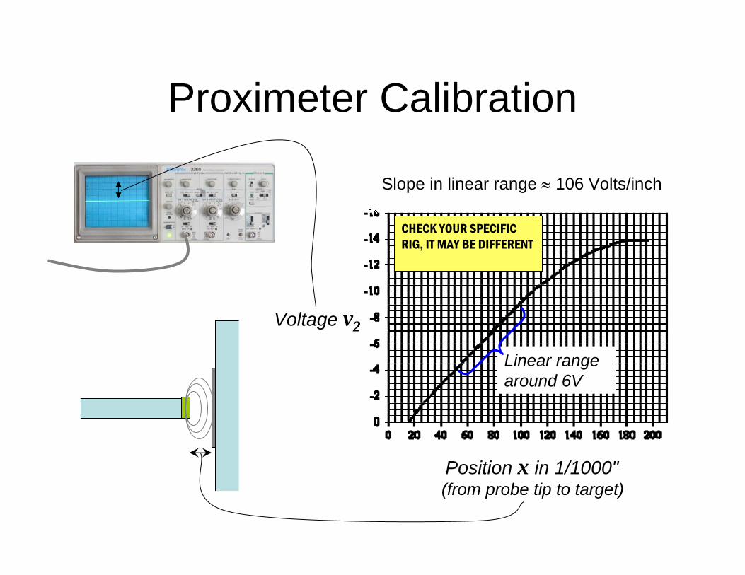
Proximeter Calibration

Voltage v2

Position x in 1/1000"(from probe tip to target)

Linear range around 6V

Slope in linear range ≈ 106 Volts/inch

CHECK YOUR SPECIFIC RIG, IT MAY BE DIFFERENT

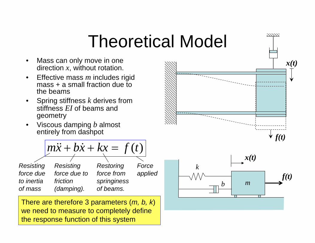
Theoretical Model• Mass can only move in one

direction x, without rotation.• Effective mass m includes rigid

mass + a small fraction due to the beams

• Spring stiffness k derives from stiffness EI of beams and geometry

• Viscous damping b almost entirely from dashpot

f(t)

x(t)

k

b m

x(t)

f(t)

)(tfkxxbxm =++ &&&

Force applied

Restoring force from springiness of beams.

Resisting force due to friction (damping).

Resisting force due to inertia of mass

There are therefore 3 parameters (m, b, k) we need to measure to completely define the response function of this system

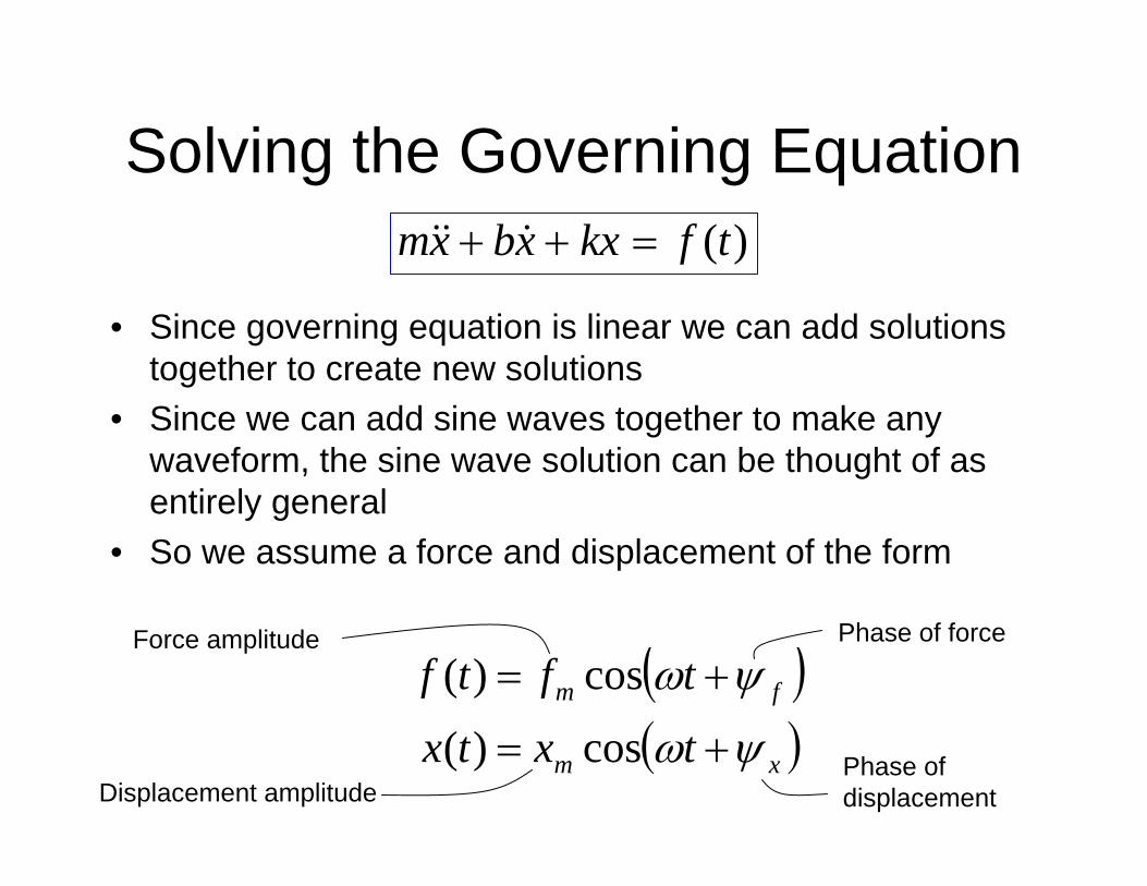
Solving the Governing Equation

• Since governing equation is linear we can add solutions together to create new solutions

• Since we can add sine waves together to make any waveform, the sine wave solution can be thought of as entirely general

• So we assume a force and displacement of the form

)(tfkxxbxm =++ &&&

( )( )xm

fm

txtx

tftf

ψω

ψω

+=

+=

cos)(

cos)(Force amplitude

Displacement amplitude

Phase of force

Phase of displacement

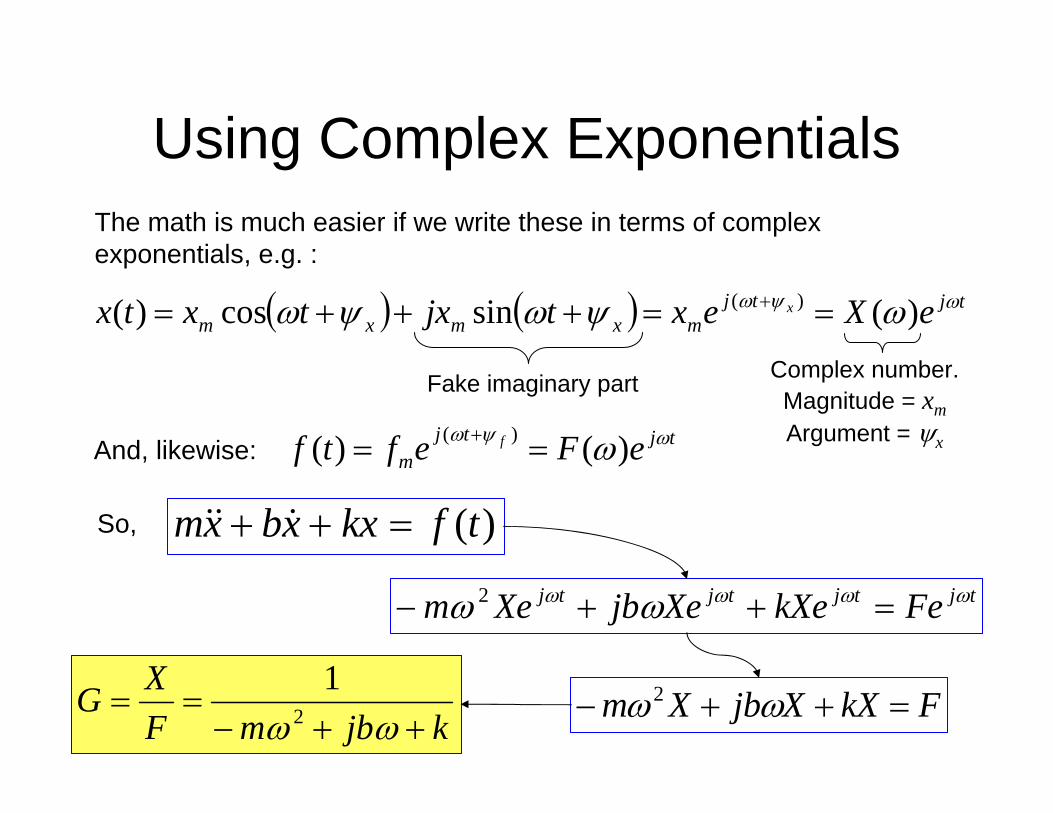
Using Complex ExponentialsThe math is much easier if we write these in terms of complex exponentials, e.g. :

( ) ( ) tjtjmxmxm eXextjxtxtx x ωψω ωψωψω )(sincos)( )( ==+++= +

Fake imaginary part Complex number.Magnitude = xmArgument = ψxAnd, likewise: tjtj

m eFeftf f ωψω ω)()( )( == +

)(tfkxxbxm =++ &&&

tjtjtjtj FekXeXejbXem ωωωω ωω =++− 2

FkXXjbXm =++− ωω2

kjbmFXG

++−==

ωω 2

1

So,

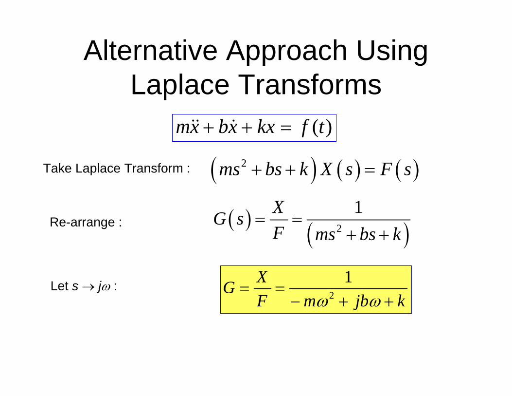
Alternative Approach Using Laplace Transforms

)(tfkxxbxm =++ &&&

( ) ( ) ( )2ms bs k X s F s+ + =

( ) ( )2

1XG sF ms bs k

= =+ +

Take Laplace Transform :

Re-arrange :

Let s → jω :kjbmF

XG++−

==ωω2

1

Response Function Solution

m

m

fx

bmkFX

=+−

=2222 )(

1ωω

mfxmkb

FX ψψψ

ωω

≡−=⎟⎠⎞

⎜⎝⎛

−−=⎟

⎠⎞

⎜⎝⎛ −

21tanarg

So, the ratio of the amplitude of the displacement to that of the force is

And the phase of the displacement relative to the phase of the force is

Phase (deg.)

0

-90

-1800 5 10 15 20 25 30 35 400

1

2

3

4

5

6

7

8x 10 -4

Frequency (Hz)

Dyn

amic

Fle

xibi

lity

(m/k

g)

Dynamic flexibility

Decreasing damping increases peak flexibility and steepens phase curve (b will be much smaller for your rig)

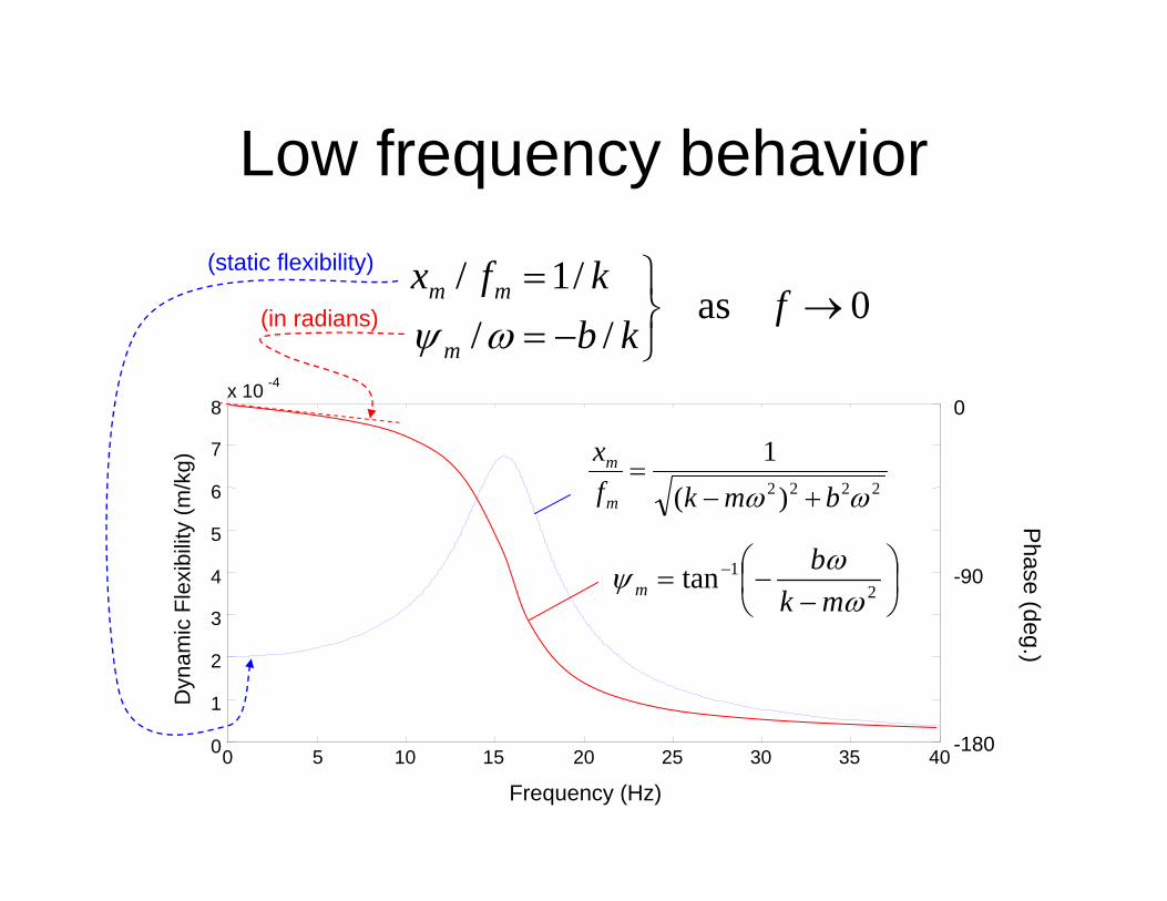
Low frequency behaviorPhase (deg.)

0

-90

-1800 5 10 15 20 25 30 35 400

1

2

3

4

5

6

7

8x 10 -4

Frequency (Hz)

Dyn

amic

Fle

xibi

lity

(m/k

g)

2222 )(1

ωω bmkfx

m

m

+−=

⎟⎠⎞

⎜⎝⎛

−−= −

21tan

ωωψmk

bm

0as//

/1/→

⎭⎬⎫

−==

fkb

kfx

m

mm

ωψ

(static flexibility)

(in radians)

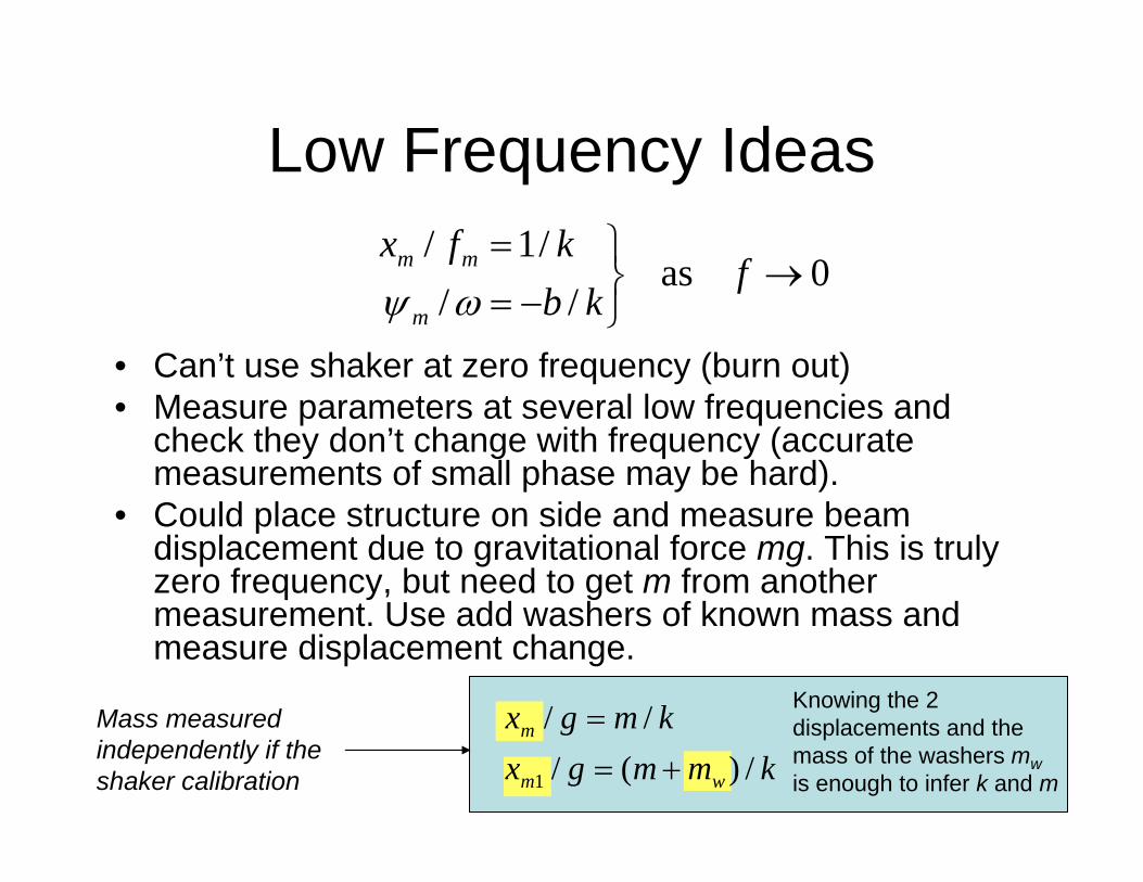
Low Frequency Ideas

• Can’t use shaker at zero frequency (burn out)• Measure parameters at several low frequencies and

check they don’t change with frequency (accurate measurements of small phase may be hard).

• Could place structure on side and measure beam displacement due to gravitational force mg. This is truly zero frequency, but need to get m from another measurement. Use add washers of known mass and measure displacement change.

0as//

/1/→

⎭⎬⎫

−==

fkb

kfx

m

mm

ωψ

kmmgxkmgx

wm

m

/)(///

1 +==

Knowing the 2 displacements and the mass of the washers mwis enough to infer k and m

Mass measured independently if the shaker calibration

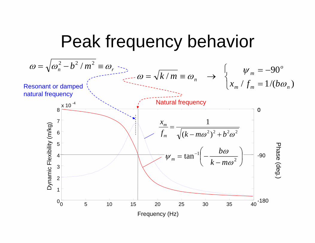
Peak frequency behaviorPhase (deg.)

0

-90

-1800 5 10 15 20 25 30 35 400

1

2

3

4

5

6

7

8x 10 -4

Frequency (Hz)

Dyn

amic

Fle

xibi

lity

(m/k

g)

2222 )(1

ωω bmkfx

m

m

+−=

Resonant or damped natural frequency

Natural frequency0

⎩⎨⎧

=−=

→≡=)/(1/

90/

nmm

om

n bfxmk

ωψ

ωωrn mb ωωω ≡−= 222 /

⎟⎠⎞

⎜⎝⎛

−−= −

21tan

ωωψmk

bm

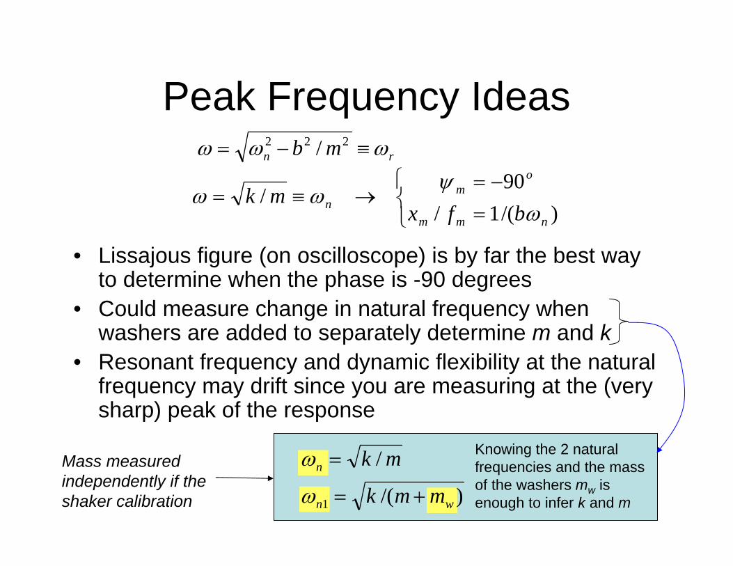
Peak Frequency Ideas

• Lissajous figure (on oscilloscope) is by far the best way to determine when the phase is -90 degrees

• Could measure change in natural frequency when washers are added to separately determine m and k

• Resonant frequency and dynamic flexibility at the natural frequency may drift since you are measuring at the (very sharp) peak of the response

⎩⎨⎧

=−=

→≡=)/(1/

90/

nmm

om

n bfxmk

ωψ

ωω

rn mb ωωω ≡−= 222 /

)/(

/

1 wn

n

mmk

mk

+=

=

ω

ω Knowing the 2 natural frequencies and the mass of the washers mw is enough to infer k and m

Mass measured independently if the shaker calibration

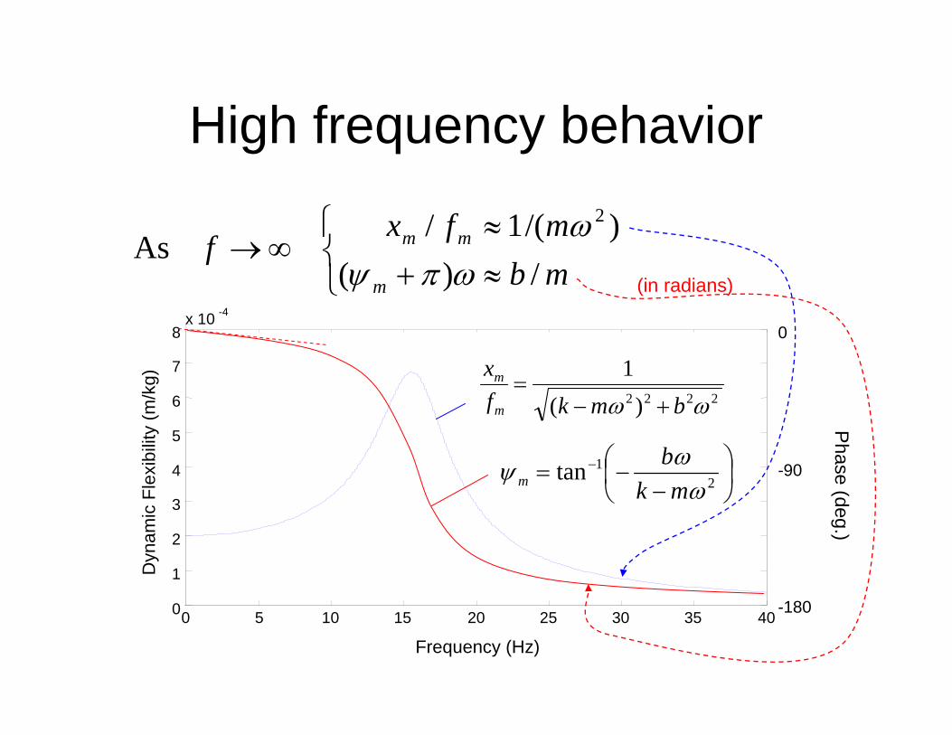
High frequency behaviorPhase (deg.)

0

-90

-1800 5 10 15 20 25 30 35 400

1

2

3

4

5

6

7

8x 10 -4

Frequency (Hz)

Dyn

amic

Fle

xibi

lity

(m/k

g)

2222 )(1

ωω bmkfx

m

m

+−=

⎟⎠⎞

⎜⎝⎛

−−= −

21tan

ωωψmk

bm

⎩⎨⎧

≈+≈

∞→mbmfx

fm

mm

/)()/(1/

As2

ωπψω

(in radians)

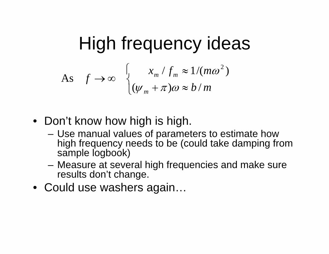
High frequency ideas

• Don’t know how high is high. – Use manual values of parameters to estimate how

high frequency needs to be (could take damping from sample logbook)

– Measure at several high frequencies and make sure results don’t change.

• Could use washers again…

⎩⎨⎧

≈+≈

∞→mbmfx

fm

mm

/)()/(1/

As2

ωπψω

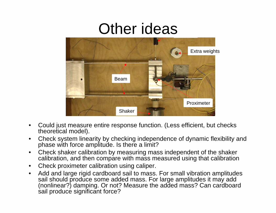
Other ideas

• Could just measure entire response function. (Less efficient, but checks theoretical model).

• Check system linearity by checking independence of dynamic flexibility and phase with force amplitude. Is there a limit?

• Check shaker calibration by measuring mass independent of the shaker calibration, and then compare with mass measured using that calibration

• Check proximeter calibration using caliper.• Add and large rigid cardboard sail to mass. For small vibration amplitudes

sail should produce some added mass. For large amplitudes it may add (nonlinear?) damping. Or not? Measure the added mass? Can cardboard sail produce significant force?

Beam

ShakerProximeter

Extra weights

Preparing for lab

• Need to come up with your own approach using these schemes and ideas, or any others you can devise.

• Few of the schemes have been tried, so some may not be practical.

• Can use ballpark estimates of parameters (based on the manual or sample logbook, say) and uncertainty analysis, to weed out truly impractical approaches before the lab.