Measuring and understanding brand value in a

dynamic model of brand management∗

Ron N. Borkovsky† Avi Goldfarb‡ Avery M. Haviv§ Sridhar Moorthy¶

May 27, 2016

Abstract

We develop a structural model of brand management to estimate the value of a brand

to a firm. In our framework, a brand’s value is the expected net present value of future

cash flows accruing to a firm due to its brand; our brand value measure recognizes that

a firm can change its brand equity by investing in advertising. We estimate quarterly

brand values in the stacked chips category for the period 2001–2006, and explore how

those values change over time. Comparing our brand value measure to its static coun-

terpart, we find that a static measure, which ignores advertising and its ability to affect

brand equity dynamics, yields brand values that are artificially high and that fluctuate

too much over time. We also explore how changing the ability to build and sustain

brand equity affects brand value. At our estimated parameterization, when brand eq-

uity depreciates more slowly, or when advertising becomes more effective at building

brand equity, brand value increases. However, counterintuitively, we find that when the

effectiveness of advertising is sufficiently high, increasing the rate at which brand equity

depreciates increases the value of a firm’s brand, even as it reduces the value of the firm

overall.

∗We are grateful for comments from Victor Aguirregabiria, Lanier Benkard, Eyal Biyalogorsky, BryanBollinger, J.P. Dube, Ron Goettler, Delaine Hampton, Gunter Hitsch, Mitsuru Igami, Przemek Jeziorski,Ahmed Khwaja, Randall Lewis, Mitch Lovett, Carl Mela, Harikesh Nair, the editors and reviewers of thisjournals, and audiences at Emory University, Stanford University, UC-Berkeley, UCLA, the University ofRochester, the University of Toronto, the 2012 UNC Branding Conference, the 2012 Marketing ScienceConference, the 2012 Marketing Dynamics Conference, the 2013 UTD-FORMS Conference, the 2013 YaleMIO Conference, the 2013 ET Symposium, the 2013 QME Conference, and the 2013 Marketing in IsraelConference. We gratefully acknowledge financial support from SSHRC Grant 410-2011-0356. We thankMarina Milenkovic for superb research assistance. This paper was previously circulated under the title “Anempirical study of the dynamics of brand building”.

†Rotman School of Management, University of Toronto, ron.borkovsky@rotman.utoronto.ca‡Rotman School of Management, University of Toronto, avi.goldfarb@rotman.utoronto.ca§Simon Business School, University of Rochester, avery.haviv@simon.rochester.edu¶Rotman School of Management, University of Toronto, sridhar.moorthy@rotman.utoronto.ca

1 Introduction

Brand equity is a key asset in the marketing of goods and services. Consumers use it

to choose among products and services, and firms see it as a summary verdict on their

marketing efforts. By its very nature, brand equity is a dynamic concept. It takes time to

build brand equity and to sustain it. By the same token, once built, brand equity doesn’t

deplete right away. Consumers continue to appreciate brand equity long after it has been

created (Keller 2008, Ataman, Mela & van Heerde 2008, Erdem, Keane & Sun 2008).

In this paper we develop a structural model of brand management and use it to estimate

the value of a brand from data on prices, advertising, and sales. We follow Goldfarb, Lu &

Moorthy (2009) in distinguishing between brand equity and brand value. The former refers

to the extra utility consumers derive from a product because of its brand identity; the latter

refers to the net present value of cash flows accruing to a firm due to its brand equity. What

distinguishes the present paper from others in the literature is that we situate the problem

of brand value measurement within a dynamic model of brand management. Our firms are

forward-looking and actively manage their brands. Specifically, they invest in advertising to

sustain or enhance brand equity while accounting for brand equity depreciation, competitive

reaction, and changes in market structure over time. Brand value in this framework thus

captures what a brand’s current equity is worth while accounting for opportunities available

to managers to change brand equity. Our structural model allows us to examine how brand

value evolves in response to changes in brand equity and in firms’ abilities to build and

sustain brands.

Our data come from the stacked potato chip industry in the period 2001–2006. During

this period, the industry was in transition. Until the fourth quarter of 2003, it was a

monopoly, with Procter & Gamble’s Pringles as the only brand. Then STAX entered as a

brand extension of Lay’s, and it became a duopoly. The industry shows interesting dynamics

in both its monopoly and duopoly periods in terms of changes in market shares, prices, and

advertising.

We take advantage of these variations to estimate Pringles and STAX brand equities

every quarter using the structural methods in Goldfarb et al. (2009), and cast the resulting

brand equities in a Pakes & McGuire (1994)-style quality ladder model to capture the

dynamics of brand management. In the quality ladder model, in each period, firms take

stock of their existing brand equities and invest in advertising to sustain and enhance brand

equity. Our brand value measure incorporates the immediate costs associated with these

advertising decisions, as well as the benefits they yield in the short- and long-run.

In 2001, at the beginning of our data set, we estimate the value of the Pringles brand

to be $2.1 billion. This value slowly declines until STAX enters. It drops immediately

by $137 million upon STAX’s entry, even though Pringles’s brand equity doesn’t change,

because increased competition limited Procter & Gamble’s ability to generate profits from

the brand. Pringles’s brand value stabilizes after STAX enters, and in the second quarter

2

of 2006—the last period of our data—it is worth $1.6 billion. Meanwhile, STAX’s brand

value, which is always below Pringles’s, declines steadily and at the end of our data it is

worth $692 million. (We show that a static measure that fails to account for advertising

and accordingly brand equity dynamics, e.g., Goldfarb et al. (2009), yields brand values

that are much higher and fluctuate much more over time.)

Our final set of results examines how changes in the ability to build and sustain brand

equity affect brand value. To vary the ability to build and sustain brand equity, we change

the brand equity depreciation rate and the effectiveness of advertising. At our estimated

parameterization, as might be expected, when brand equity depreciates more slowly, or

when advertising becomes more effective at building brand equity, brand value increases.

However, there is a counterintuitive interaction effect between the two: When the ef-

fectiveness of advertising is sufficiently high, there is an inverted-U shaped relationship

between the brand equity depreciation rate and brand value. It follows that increasing the

brand equity depreciation rate increases brand value, even as it (expectedly) reduces the

value of the firm overall. So, a firm’s brand becomes more valuable even as the brand equity

that underpins it becomes harder to sustain. When the brand equity depreciation rate is

low, a brand’s value is relatively low because the brand equity that it possesses would be

rebuilt relatively easily if it were lost. When the depreciation rate is high, a brand’s value is

also relatively low because the brand equity that it possesses cannot be sustained. A brand

is most valuable at intermediate depreciation rates because the brand equity that it pos-

sesses can be sustained—and therefore generates high profit for the firm—and were it lost,

it would be very time-consuming to rebuild. In summary, when advertising is sufficiently

effective, a brand is most valuable when the brand equity depreciation rate is neither too

low nor too high.

2 Issues in measuring brand value

In motivating our approach to measuring brand value, we emphasize the underlying goal of

measuring the financial value of a brand to the parent firm. The emphasis on brand means

that we need to separate out the contribution of the brand itself from what the product

(including the brand) actually achieves in the marketplace (Keller 2008, p. 48; Fischer

2007). This calls for a comparison between a “factual” and a “counterfactual.” Hence, we

define brand value as the difference between the expected net present value of cash flows

in a factual scenario—in which a product possesses its brand equity—and a hypothetical

counterfactual scenario—in which the product is stripped of its brand equity. In both

scenarios, firms retain the ability to brand build, hence in the factual scenario a firm can

strive to sustain or enhance its brand equity, and in the counterfactual scenario a firm can try

to rebuild its brand equity anew. Furthermore, because factual and counterfactual pricing

and ad spending decisions are determined by an equilibrium, we model those decisions for

each firm in every period, taking into account the prevailing brand equity levels of all firms

3

in the industry.

Earlier approaches to measuring brand value have captured some parts of this conceptual

framework, but not all. For instance, Barwise, Higson, & Likierman (1989), Simon &

Sullivan (1993), and Fischer (2007) acknowledge the need to measure the discounted present

value of cash flows generated by the brand, but do not perform a full analysis of the

counterfactual scenario that accounts for the impact of the brand on both consumer and

firm behavior. Others incorporate a counterfactual scenario in which a firm is stripped of its

brand and in which all firms change their behavior accordingly (Goldfarb et al. 2009, Ferjani,

Jedidi & Jagpal 2009), but do so in a static setting that does not account for brand building.

Fischer (2007) lists six features of an ideal measure of brand value: completeness, compa-

rability, objectivity, future orientation, cost-effectiveness, and simplicity. While our method

is not simple and it is hard to assess cost effectiveness at this point, we believe that it has

important strengths in terms of the other four features.

First, a measure of brand value is regarded as complete only if it accounts for both the

price premium and the volume premium that a firm enjoys because of its brand.1 This

encapsulates the broader point made above, i.e., that a measure must properly account

for the benefits that a product (including the brand) enjoys relative to a hypothetical

unbranded version of the product. Our measure captures the price and volume premiums.

Furthermore, our approach suggests that the interpretation of completeness described above

is itself incomplete because it fails to account for the effect of a firm’s brand on brand

building decisions and accordingly the evolution of the industry over time.

Second, comparability refers to the ability of an approach to yield brand value mea-

sures that can be compared across industries and over time. To satisfy this criterion, an

approach must not give rise to unwarranted intertemporal fluctuations in a brand’s value.

Our approach gives rise to brand values that are relatively stable over time. Furthermore,

our results show that failing to account for the effect of the brand on firms’ forward-looking

brand building decisions can indeed give rise to wide fluctuations in a brand value measure

that are not reflective of the true value of the brand.

Third, our approach is objective in that we use standard data on prices, sales, and

ad spending, and we provide a general framework for measuring brand value that can be

adapted to suit a wide variety of industries and product categories. Finally, by definition,

our approach satisfies the future-oriented criterion.

In addition to strengths that build on and improve the state of the art in the prior

academic literature, we also see considerable advantages to our approach relative to using

the brand values calculated by brand consulting firms. In particular, each consultancy

1Rosen (1974), Holbrook (1992), and Swait, Erdem, Louviere & Dubelaar (1993) estimate brand equityusing a price premium approach. Kamakura & Russell (1993) and Srinivasan, Park & Chang (2005) estimatebrand equity using a volume premium approach. Srinivasan & Park (1997) estimates brand equity using bothapproaches. Ailawadi, Lehmann & Neslin (2003) measure brand value using a revenue premium approach,which accounts for both the price and volume premiums.

4

uses its own approach, and none fully reveals its methodology.2 As with other approaches

in the academic literature, our approach has the advantage of being transparent. These

brand consultancy approaches also are not complete in the sense that they do not formally

consider a counterfactual scenario that explores how the absence of a brand would impact

the decision-making of consumers and firms. The brand consultancy approaches may also

be less objective to the extent that the results rely on less objective data sources (surveys,

focus groups, or expert panels). Therefore, relative to the brand consulting approaches, we

offer a methodology that is transparent and that can therefore be more easily appraised,

applied, and augmented.

A further advantage of our method is that it can be seen as valuing the brand asset

with a real options approach rather than a net present value approach (Dixit & Pindyck

1994), accounting for the irreversibility of investment decisions (in brand building) and

the uncertainty of the economic environment. In finance, it is now widely recognized that

assets should be valued using a real options approach because failing to account for all of

the possible future paths down which the economic environment might evolve can lead to

incorrect valuations (see Dixit & Pindyck 1994, p. 6). In this way, we measure brands as

assets in a way consistent with contemporary thinking on how assets should be valued.

3 Category description and data

In this section, we describe the stacked chips category and the data that we use to estimate

our model.

3.1 Category

The stacked chips category originated in the late 1960s when Procter & Gamble (P&G)

introduced Pringles. P&G’s plan was to distribute Pringles over its existing distribution

network, which was optimized for non-perishable products. To ensure that the chips didn’t

spoil in transit, they were to be packed in nitrogen, which necessitated an airtight seal. This

led to the now-familiar cylindrical containers and the uniformly-shaped chips that could be

stacked in them.3 By the mid-1990s, Pringles had $1 billion in annual sales. In 2012 (after

our data period), Pringles was sold to Kellogg’s for about $2.7 billion (de la Merced 2012).

Frito-Lay, a division of PepsiCo, launched Lay’s STAX in 2003. Like Pringles, STAX

chips are stacked and packaged in cylindrical containers. STAX was launched with sub-

stantial marketing support, spending more on advertising than Pringles in the first quarter

2Interbrand, WPP/Millward Brown, and Prophet use discounted cash flow techniques based on theeconomic profits attributable to the brand. Brand Finance uses a discounted cash flow approach that ismore transparent because it is based on royalties that a firm would have to pay were it stripped of its brand.BAV and CoreBrand use measures that are largely survey-based. Because the various methods are valuableintellectual property, the details of how the values are derived are not public.

3Frederic J. Baur was so proud of having invented the Pringles container that he asked that his ashes beburied in one. When he died in 2008, his children honored his wish (Caplan 2008).

5

after entry. It immediately gained about 20% market share of the stacked chips category.

We treat stacked chips as a distinct category. We allow demand for other salty snacks

brands in chips, pretzels, popcorn, and cheese snacks to affect demand for stacked chips

(as the outside good in a nested model) but focus on competition and strategic interaction

between Pringles and STAX. We do this partly for convenience (the duopoly setting is

needed for estimation) but we believe it is reasonable given the close substitutability of the

two stacked chips brands.

3.2 Data

Our data come from the IRI Marketing Data Set (Bronnenberg, Kruger & Mela 2008),

which provides weekly data at the product level for 2664 participating stores in 47 U.S.

markets, between January 1, 2001 and December 31, 2006. Our quarterly estimate of brand

equity is based on a static pricing game at the week level and is estimated using data at the

store-week-brand level. Our estimate of brand value uses the quarter-brand as the unit of

observation and emphasizes quarterly advertising spending data and the quarterly estimates

of brand equity derived from the static game.

This data set is well-suited for this project for several reasons. First, it is very detailed:

for each store and each week, the volume and average purchase price are reported. These

variables are necessary for estimating brand equity (Goldfarb et al. 2009). Second, besides

the entry of a new brand, we observe interesting dynamics in advertising, prices, and market

shares throughout the data period, both in the monopoly phase and in the duopoly phase.

The variations in market share and advertising allow us to identify the dynamic parameters

in our model. Third, the IRI Marketing Data Set contains quarterly advertising spending

data (primarily estimated through a media audit) for each brand in the category (provided

by TNS Custom Research), spanning the period January 1, 2001–June 30, 2006.

3.3 Descriptive statistics

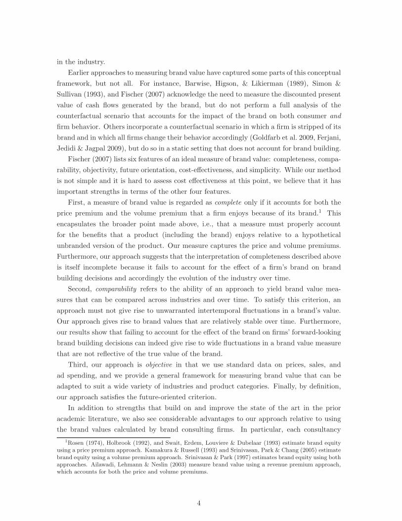
Table 1 provides descriptive statistics for the 22 (resp. 11) quarters in which Pringles (STAX)

is active in our data set,4 and Figure 1 presents plots of market shares, average price,

and advertising spending. The bottom panel of Figure 1 shows substantial variability in

quarterly ad spending for both brands. The upper-left panel of Figure 1 shows that market

shares are more stable than advertising, although they also vary quite a bit over time. The

upper-right panel of Figure 1 shows that STAX’s prices are below Pringles, with the gap

increasing from almost zero in the fourth quarter of 2003 to close to 20% in the first quarter

of 2006.

4Here and elsewhere, all dollar amounts are deflated to year-2000 dollars using the Consumer Price Index.

6

0%

2%

4%

6%

8%

10%

12%

14%

16%

18%

20%

Quarter

Mar

ket S

hare

2001

−Q1

2002

−Q1

2003

−Q1

2004

−Q1

2005

−Q1

2006

−Q1

PringlesSTAX

0.9

1

1.1

1.2

1.3

1.4

1.5

Quarter

Ave

rage

Pric

e (D

olla

rs)

2001

−Q1

2002

−Q1

2003

−Q1

2004

−Q1

2005

−Q1

2006

−Q1

0

2

4

6

8

10

12

14

16

18

Quarter

Adv

ertis

ing

(Mill

ions

of D

olla

rs)

2001

−Q1

2002

−Q1

2003

−Q1

2004

−Q1

2005

−Q1

2006

−Q1

Figure 1: Market shares (in chips, pretzels, popcorn, and cheese snacks categories), averageprices, and advertising spending.

4 The static period game

We conceptualize firms as making two types of decisions, short-run and long-run. The

short-run decisions are in prices, made weekly at each store. The long-run decisions are

in advertising, and they are made quarterly at the national level.5 We denote the week

by t and the quarter by q. By “static period game” we mean the weekly competition in

prices between the two firms; by “dynamic game” we mean the quarterly competition in

advertising.

The static and dynamic character of these games comes from our assumption that firms

behave as if brand equities are fixed in the short-run, unaffected by prices, but changeable

in the long-run, through natural forces such as depreciation, and choices such as advertising.

5This assumption is based on institutional evidence that advertising budgets were confirmed quarterlyin the period 2001–2006 (interview with former P&G VP with detailed knowledge of the Pringles businessduring that time period who wishes to remain anonymous, August 2012).

7

Mean SD Min Max

Pringles

Advertising ($ millions per quarter) 8.76 4.16 1.56 17.62Average price per quarter ($) 1.28 0.11 1.12 1.52Market share (of chips, pretzels, popcorn, and cheese snacks) 0.15 0.01 0.12 0.18Sales ($ millions per quarter) 4.74 0.43 3.92 5.42

STAX

Advertising ($ millions per quarter) 4.01 4.73 0.00 12.56Average price per quarter (dollars) 1.08 0.09 0.98 1.25Market share (of chips, pretzels, popcorn, and cheese snacks) 0.04 0.01 0.03 0.04Sales ($ millions per quarter) 1.12 0.12 0.93 1.28

Table 1: Descriptives statistics.

This is as if the firm is investing quarterly and harvesting weekly.

This division between the short-run and the long-run, with brand equities fixed in the

short-run and changeable in the long-run, is central to our empirical estimation strategy. We

believe that it is also reasonable. We do expect brand equities to be relatively immoveable

objects—if they were not, they wouldn’t be “assets.” But at the same time, they are not

fixed forever; depreciation takes its toll, and advertising can build and restore brand equity

over the long run. Consistent with this framing, we model price choices as weekly and

advertising choices as quarterly.

Methodologically, thinking of the period game as a static game allows us to use weekly

store data on sales and prices to estimate demand-side and supply-side parameters, in

particular, Pringles and STAX brand equities and firms’ marginal costs. This allows us

to estimate the period profit function. The estimated brand equities and the period profit

function are then taken to the dynamic game described in Section 4; here, the brand equities

at the beginning of a quarter serve as “start states,” which depreciate during the quarter,

and advertising decisions are made to achieve desirable “end states.”6

4.1 Model

We estimate demand in a nested logit framework. As noted earlier, the structure of the

stacked chips industry changed during 2001–2006, from monopoly in the first half to duopoly

in the second half. Still, because we seek to model STAX’s entry decision, we need to analyze

the industry as if it were a duopoly from the beginning, comprising an incumbent firm and

a potential entrant.

Our data cover 2664 stores. We account for differences across stores by assuming that

6In previous applications of the Ericson & Pakes (1995) framework, states have typically been observed inthe data. For example, in the Goettler & Gordon (2011) study of R&D competition between Intel and AMD,the authors observe processor speed (their state variable). In our study, brand equities at the beginning ofa quarter serve as the state variables for the dynamic game in that quarter, but we don’t observe them inthe data; therefore we need to estimate them prior to estimating the dynamic model.

8

stores have different market sizes and firm-specific shocks. A firm’s marginal cost varies

across stores, reflecting differences in transportation costs and/or trade promotions. We

incorporate this store-level heterogeneity by assuming that each store in each period draws

its market size, firm-specific shocks, and firm-specific marginal costs from the same distri-

butions. We explain below how we estimate these distributions.7

As explained above, we assume that firms in our model set weekly prices at the store-

level. While firms in reality do not set separate prices for each and every store, this as-

sumption simplifies our model and allows us to account for the store-level heterogeneity

described above. We feel that this a reasonable approach, especially given that our goal is

to estimate the distributions of market sizes, firm-level shocks, and marginal costs that are

common to all stores, as opposed to store-level distributions.8

There are two firms in our model, n = 1, 2, competing weekly in prices in each store,

taking their brand equities as given. This is vertically-differentiated price competition be-

cause one brand typically has more equity than the other. Let ωn ∈ {0, 1, . . . ,M} represent

the state of firm n ∈ {1, 2} in a given quarter. States 1, . . . ,M describe the brand eq-

uity of a firm that is active in the product market, i.e., an incumbent firm, while state 0

identifies a firm as being inactive, i.e., a potential entrant. This formulation allows us to

simultaneously capture situations in which both brands are active and situations in which

only one brand is active. Thus, in the data, Pringles’s state will always be one of 1, . . . ,M ,

whereas STAX’s state will be 0 in the weeks leading up to its entry. The industry state is

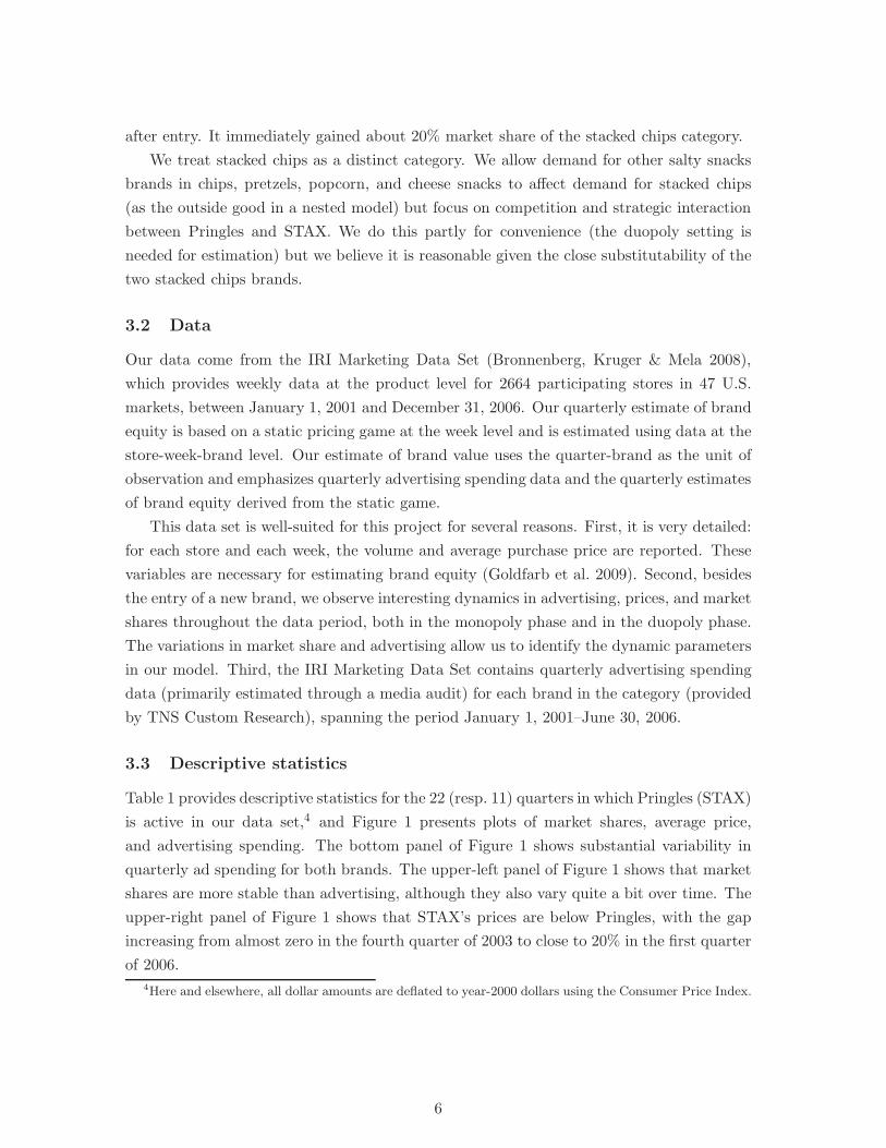
ω = (ω1, ω2) ∈ {0, . . . ,M}2.There is a continuum of consumers in the market. Each consumer purchases at most one

unit of one product in each week. The utility that consumer i shopping at store j derives

from purchasing from firm n is

uijn(ωn) = B(ωn)− κpjn + ζjn + ξij + (1− σ)εijn, (1)

7Alternatively, we could have estimated these distributions at the store-level. The benefit of our approachis that it allows us to incorporate store-level heterogeneity without increasing the computational burdensubstantially—we simply approximate the expected profit function by integrating out over the aforemen-tioned distributions using Monte Carlo simulation. Had we estimated those distributions at the store-level,we would have had to conduct this same exercise for each store. This approach would significantly increasethe computational burden of both the period profit approximation and the calculation of standard errors ofthe dynamic model. In fact, because we calculate standard errors of the dynamic model using a parametricbootstrap with 100 bootstrap samples, and for each bootstrap sample we approximate a separate periodprofit function, this approach to computing standard errors would be computationally infeasible.

8We are abstracting away from the role of the retailer. Effectively we are assuming that the retail sectoris perfectly competitive, which is likely reasonable for grocery retailing. Our assumption has the virtueof reducing the computational burden of estimating the model and running counterfactuals. Alternatively,we could have assumed a monopolistic retailer, as in Sudhir (2001) and Goldfarb et al. (2009). However,because brand equity states are derived exclusively from retail prices and market shares, changing theindustry structure at the retail level would not affect the brand equity states that we estimate in the firststage. What would change is the period profit function. In principle, our framework can be applied usingwhichever assumption about industry structure at the retail level is most appropriate for the application athand.

9

where B : (0, 1, . . . ,M) → R is an increasing function that maps brand equity state ωn into

brand equity B(ωn). We specify B(ωn) in Section 5 below. (Even though we distinguish

between brand equity states ωn and brand equities B(ωn), for ease of exposition we will

sometimes refer to ωn as “brand equity.”) pjn is firm n’s price in store j, ζjn is a mean

zero firm-store-specific shock (to accommodate unobserved heterogeneity across firms and

stores) with standard deviation σζ , and ξij + (1− σ)εijn is an individual error term, where

ξij is the idiosyncratic propensity of consumer i to make a purchase in store j, and σ ∈ [0, 1)

determines the extent to which consumers’ preferences for the firms’ products are correlated.

We set B(0) = −∞ to ensure that potential entrants have zero demand, and hence do not

compete in the product market. There is an outside alternative, product 0, which has

utility

uij0 = ξ′ij + (1− σ)εij0. (2)

Assuming that the idiosyncratic preferences εij0, εij1, and εij2 have independent and identi-

cally distributed type-1 extreme value distributions, and that ξij and ξ′ij have distributions

depending on σ such that ξij + (1− σ)εijn and ξ′ij + (1 − σ)εij0 have extreme value distri-

butions, the demand for incumbent firm n’s product in store j is

Djn(pj ;ω,mj, ζj) = mj

exp(

B(ωn)−κpjn+ζjn1−σ

)

Cj + Cσj, (3)

and the demand for the outside good is

Dj0(pj ;ω,mj , ζj) = mj

Cσj

Cj + Cσj, (4)

where pj = (pj1, pj2) is the vector of prices, κ is the price coefficient, mj > 0 is the size

of the market for store j (the sales of all chips, pretzels, popcorn, and cheese snacks),

ζj = (ζj1, ζj2) is the vector of week-store-specific shocks to consumer utility for each brand,

and Cj =2∑

n=1exp

(

B(ωn)−κpjn+ζjn1−σ

)

.9 The market sizemj is assumed to have an independent

normal distribution with mean µm and standard deviation σm. ζjn is assumed to have a

mean-zero normal distribution with standard deviation σζ .

Given industry state ω, firm n chooses price pjn to maximize its weekly profit from store

j:

πjn(ω, cjn,mj , ζj) = maxpjn

Dn((pjn, pj,−n);ω,mj , ζj)(pjn − cjn), (5)

where pj,−n is the price charged by its rival and cjn ≥ 0 is the marginal cost that firm n

incurs when serving store j. We assume that the marginal cost is drawn from a log-normal

distribution with mean µc and standard deviation σc and is independently and identically

distributed across stores, firms, and weeks.

9To simplify exposition, we suppress the dependence of Cj on pj , ω, and ζj .

10

By Caplin & Nalebuff (1991), there exists a unique Nash equilibrium of the period

game. We find it by solving the system of first-order conditions that arises from the firms’

profit-maximization decisions via best reply iteration. Let π∗n(ω, cj ,mj , ζj) denote firm n’s

quarterly (not weekly) equilibrium profit in store j. Integrating over market size, marginal

costs, and the firm-store specific shocks, and multiplying by the number of stores (2664)

and the number of weeks per quarter (13), we compute the expected equilibrium quarterly

profit in industry state ω as

π∗n(ω) = 2664 × 13×∫

cj ,mj ,ζj

π∗jn(ω, cj ,mj , ζj)fc(cj)fm(mj)fζ(ζj)dcjdmjdζj, (6)

where fc(cj), fm(mj), and fζ(ζj) are the probability distribution functions of cj , mj , and

ζj respectively.

4.2 Estimation

Demand function. We follow Goldfarb et al. (2009) in estimating the parameters of the

demand function. Specifically, we estimate a nested logit demand model with two nests, one

for the two stacked chips brands, Pringles and STAX, and the other for the outside good,

which includes non-stacked chips, pretzels, popcorn, and cheese snacks. This captures the

idea that brands of stacked potato chips will compete more fiercely with each other than

with other types of salty snacks.

The brand equity of each firm in each quarter is defined as the additional utility a

consumer receives from consuming a branded product versus its unbranded equivalent.

Operationally, this is represented as a brand-quarter fixed effect in the consumer’s utility

function.

Recall that the demand for good n in store j is

Djn(pjt;ωq,mjt, ζjt) = mjt

exp(B(ωnq)−κpjnt+ζjnt

1−σ )

Cjt + Cσjt,

where ωnq is firm n’s brand equity state in the quarter q that includes week t, and the

demand for the outside good is

Dj0(pjt;ωq,mjt, ζjt) = mjt

Cσjt

Cjt +Cσjt.

The market size for store j in week t, mjt, is the total number of units of all chips, pretzels,

popcorn, and cheese snacks sold in store j in that week. We do not observe the entire U.S.

market in the IRI database because it includes a sample of U.S. drug and grocery stores in

a subset of U.S. markets. So we approximate the size of the full U.S. market as follows. We

first compute average weekly household spending on all chips, pretzels, popcorn, and cheese

snacks in drug and grocery stores by multiplying average weekly household spending on all

11

salty snacks in such stores (from Bronnenberg et al. 2008) by the percentage of total salty

snack spending that is constituted by chips, pretzels, popcorn, and cheese snacks (computed

from the IRI database). We multiply this by the total number of U.S. households to get

total U.S. spending on all four of these salty snack categories in drug and grocery stores.

Because market size is defined in units (not dollars), we divide this by the average price to

get the total number of units of these salty snacks sold in drug and grocery stores. We then

multiply this by the percentage of chips, pretzels, popcorn, and cheese snacks sales in the

IRI database that are from grocery stores, rather than drug stores (97.95%) to estimate the

size of the market in grocery stores. Finally, to obtain the size of the full market, which

includes grocery stores, drug stores, mass stores, convenience stores, and club stores, we

scale up our estimate based on a report from P&G that implies that grocery makes up 25%

of Pringles’s sales10. We divide by the number of stores in our data, yielding an estimate

of µm = 342, 463.04 units, implicitly scaling up the market size of each store in the data so

that the stores collectively represent the entire U.S. market.11

Taking the difference between the log market shares of firm n in store j and the outside

good in store j, we have:

log(

Djn(pjt;ωq,mjt,ζjt)

mjt

)

−log(

Dj0(pjt;ωq ,mjt,ζjt)

mjt

)

= B(ωnq)−κpjnt+σ log(

Djn(pjt;ωq,mjt,ζjt)

mjt−Dj0(pjt;ωq,mjt,ζjt)

)

+ζjnt.

Ordinary least squares (OLS) estimation of the above expression would be biased due to

the endogeneity of price (it is possible that firms observe ζjnt before setting prices) and

the inside share. Following Nevo (2001), we use the price of the brand in other cities, the

price of the brand in other stores in the same store chain, and the price of the brand in

other stores in the same chain and city as instruments. For these to be valid instruments,

the stores in other cities and other stores in the chain must share a cost shock, but have

distinct demand shocks. Our results are presented in Table 2 and Figure 2, the latter being

a plot of the estimated brand equities of Pringles and STAX quarter by quarter, along with

a discretization of the brand equity continuum that is described in Section 5.

Marginal costs. Given the estimates of κ and σ, we can compute the marginal cost

for each store-firm-week combination from the first-order condition describing the price

equilibrium:

cjnt = pjnt −1− σ

κ(

1− sjnt

(

1 + σsj0t

1−sj0t

)) , (7)

where sjnt and sj0t are the shares of firm n and the outside good respectively in store j in

week t that are observed in the data. We can then estimate µc and σc using the first and

10See http://www.pg.com/en_US/downloads/investors/investor_presentation.pdf .11We need not estimate σm because the market size mj enters the demand function (3) multiplicatively

and is independent of all other model parameters. It follows that µm is multiplicatively separable from therest of the profit function (6). Therefore, in approximating the profit function, we can simply replace mj

with its expectation µm.

12

Quarter Pringles Brand STAX Brand Quarter Pringles Brand STAX BrandEquity Equity Equity Equity

2001-Q1 0.893∗∗∗ n/a 2004-Q1 0.698∗∗∗ −0.009(0.007) (0.006) (0.007)

2001-Q2 0.758∗∗∗ n/a 2004-Q2 0.566∗∗∗ −0.105∗∗∗

(0.007) (0.006) (0.007)2001-Q3 0.841∗∗∗ n/a 2004-Q3 0.727∗∗∗ 0.033∗∗∗

(0.007) (0.006) (0.007)2001-Q4 0.692∗∗∗ n/a 2004-Q4 0.673∗∗∗ −0.116∗∗∗

(0.007) (0.006) (0.007)2002-Q1 0.740∗∗∗ n/a 2005-Q1 0.642∗∗∗ −0.099∗∗∗

(0.007) (0.006) (0.007)2002-Q2 0.730∗∗∗ n/a 2005-Q2 0.633∗∗∗ −0.089∗∗∗

(0.007) (0.006) (0.007)2002-Q3 0.855∗∗∗ n/a 2005-Q3 0.625∗∗∗ −0.118∗∗∗

(0.007) (0.006) (0.007)2002-Q4 0.618∗∗∗ n/a 2005-Q4 0.502∗∗∗ −0.296∗∗∗

(0.007) (0.006) (0.007)2003-Q1 0.666∗∗∗ n/a 2006-Q1 0.605∗∗∗ −0.202∗∗∗

(0.007) (0.006) (0.007)2003-Q2 0.432∗∗∗ n/a 2006-Q2 0.517∗∗∗ −0.268∗∗∗

(0.007) (0.006) (0.006)2003-Q3 0.674∗∗∗ n/a 2006-Q3 0.537∗∗∗ −0.246∗∗∗

(0.007) (0.006) (0.007)2003-Q4 0.673∗∗∗ 0.072∗∗∗ 2006-Q4 0.440∗∗∗ −0.300∗∗∗

(0.006) (0.007) (0.006) (0.007)

κ (price −1.554∗∗∗

coefficient) (0.004)σ 0.616∗∗∗

(0.003)σζ 0.646∗∗∗

(0.001)

R2 0.932Adjusted R2 0.932Residual Std. Error 11.481 (df = 807,198)# of Observations 807,248

Unit of observation is the store-week. Nested logit demand. Instruments are price of thebrand in other cities, price of the brand in other stores in the same store chain, and priceof the brand in other stores in the same chain and city. Standard errors in parentheses.*p < .1, **p < .05, ***p < .01.

Table 2: Demand estimation results.

13

−1.0

−0.5

0.0

0.5

1.0

1.5

Quarter

Bra

nd E

quity

(U

tils)

2001

−Q1

2001

−Q3

2002

−Q1

2002

−Q3

2003

−Q1

2003

−Q3

2004

−Q1

2004

−Q3

2005

−Q1

2005

−Q3

2006

−Q1

PringlesSTAX

Figure 2: Brand equity over time

second sample moments of cjnt; this yields estimates of µc = 0.856 and σc = 0.180.

Expected profits. Because equilibrium prices must be computed numerically, there is

no closed-form solution for π∗n(ω). We therefore approximate the expected profit function

(6) in each industry state through Monte Carlo simulation, integrating over the estimated

distributions of cj and ζj .

The plots of expected price, expected demand, expected market share, and expected

profit are presented in Figure 3, where ω1 and ω2 are the brand equities of firms 1 and 2 (we

use the language ‘firm 1 and firm 2’—as opposed to ‘Pringles and STAX’—because firms are

symmetric, hence the results in the figure are for either Pringles or STAX). Market share,

price and accordingly profit increase relatively rapidly—and at an increasing rate—as brand

equity increases, and they decline as rival brand equity increases.

14

0

10

20

30

0

10

20

30

0

0.5

1

1.5

2

ω1

ω2

Exp

ecte

d P

rice

(Dol

lars

)

0

10

20

30

0

10

20

30

0

50

100

150

200

250

300

ω1

ω2

Exp

ecte

d Q

uant

ity D

eman

ded

(Mill

ions

)

0

10

20

30

0

10

20

30

0

0.05

0.1

0.15

0.2

0.25

0.3

ω1

ω2

Exp

ecte

d M

arke

t Sha

re

0

10

20

30

0

10

20

30

0

50

100

150

200

250

300

ω1

ω2

Exp

ecte

d P

rofit

(M

illio

ns)

Figure 3: Period game Nash equilibrium (functions presented are for firm 1, expected profitand quantity demanded are quarterly).

15

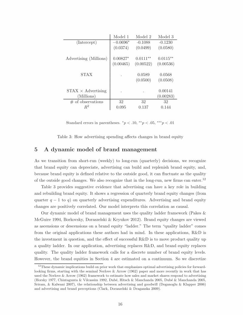
Model 1 Model 2 Model 3

(Intercept) −0.0696∗ -0.1088 -0.1230(0.0374) (0.0499) (0.0580)

Advertising (Millions) 0.00827∗ 0.0111∗∗ 0.0115∗∗

(0.00465) (0.00522) (0.00536)

STAX . 0.0589 0.0568(0.0500) (0.0508)

STAX × Advertising . . 0.00141(Millions) (0.00283)

# of observations 32 32 32R2 0.095 0.137 0.144

Standard errors in parentheses. ∗p < .10, ∗∗p < .05, ∗∗∗p < .01

Table 3: How advertising spending affects changes in brand equity

5 A dynamic model of brand management

As we transition from short-run (weekly) to long-run (quarterly) decisions, we recognize

that brand equity can depreciate, advertising can build and replenish brand equity, and,

because brand equity is defined relative to the outside good, it can fluctuate as the quality

of the outside good changes. We also recognize that in the long-run, new firms can enter.12

Table 3 provides suggestive evidence that advertising can have a key role in building

and rebuilding brand equity. It shows a regression of quarterly brand equity changes (from

quarter q − 1 to q) on quarterly advertising expenditures. Advertising and brand equity

changes are positively correlated. Our model interprets this correlation as causal.

Our dynamic model of brand management uses the quality ladder framework (Pakes &

McGuire 1994, Borkovsky, Doraszelski & Kryukov 2012). Brand equity changes are viewed

as ascensions or descensions on a brand equity “ladder.” The term “quality ladder” comes

from the original applications these authors had in mind. In these applications, R&D is

the investment in question, and the effect of successful R&D is to move product quality up

a quality ladder. In our application, advertising replaces R&D, and brand equity replaces

quality. The quality ladder framework calls for a discrete number of brand equity levels.

However, the brand equities in Section 4 are estimated on a continuum. So we discretize

12These dynamic implications build on prior work that emphasizes optimal advertising policies for forward-looking firms, starting with the seminal Nerlove & Arrow (1962) paper and more recently in work that hasused the Nerlove & Arrow (1962) framework to estimate how sales and market shares respond to advertising(Horsky 1977, Chintagunta & Vilcassim 1992, Dube, Hitsch & Manchanda 2005, Dube & Manchanda 2005,Sriram, & Kalwani 2007), the relationship between advertising and goodwill (Doganoglu & Klapper 2006)and advertising and brand perceptions (Clark, Doraszelski & Draganska 2009).

16

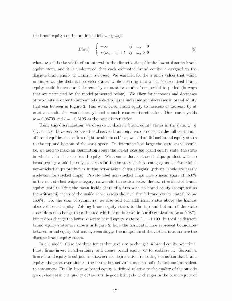
the brand equity continuum in the following way:

B(ωn) =

{

−∞ if ωn = 0

w(ωn − 1) + l if ωn > 0(8)

where w > 0 is the width of an interval in the discretization, l is the lowest discrete brand

equity state, and it is understood that each estimated brand equity is assigned to the

discrete brand equity to which it is closest. We searched for the w and l values that would

minimize w, the distance between states, while ensuring that a firm’s discretized brand

equity could increase and decrease by at most two units from period to period (in ways

that are permitted by the model presented below). We allow for increases and decreases

of two units in order to accommodate several large increases and decreases in brand equity

that can be seen in Figure 2. Had we allowed brand equity to increase or decrease by at

most one unit, this would have yielded a much coarser discretization. Our search yields

w = 0.08700 and l = −0.3196 as the best discretization.

Using this discretization, we observe 15 discrete brand equity states in the data, ωn ∈{1, . . . , 15}. However, because the observed brand equities do not span the full continuum

of brand equities that a firm might be able to achieve, we add additional brand equity states

to the top and bottom of the state space. To determine how large the state space should

be, we need to make an assumption about the lowest possible brand equity state, the state

in which a firm has no brand equity. We assume that a stacked chips product with no

brand equity would be only as successful in the stacked chips category as a private-label

non-stacked chips product is in the non-stacked chips category (private labels are nearly

irrelevant for stacked chips). Private-label non-stacked chips have a mean share of 15.6%

in the non-stacked chips category, so we add ten states below the lowest estimated brand

equity state to bring the mean inside share of a firm with no brand equity (computed as

the arithmetic mean of the inside share across the rival firm’s brand equity states) below

15.6%. For the sake of symmetry, we also add ten additional states above the highest

observed brand equity. Adding brand equity states to the top and bottom of the state

space does not change the estimated width of an interval in our discretization (w = 0.087),

but it does change the lowest discrete brand equity state to l = −1.190. In total 35 discrete

brand equity states are shown in Figure 2; here the horizontal lines represent boundaries

between brand equity states and, accordingly, the midpoints of the vertical intervals are the

discrete brand equity states.

In our model, there are three forces that give rise to changes in brand equity over time.

First, firms invest in advertising to increase brand equity or to stabilize it. Second, a

firm’s brand equity is subject to idiosyncratic depreciation, reflecting the notion that brand

equity dissipates over time as the marketing activities used to build it become less salient

to consumers. Finally, because brand equity is defined relative to the quality of the outside

good, changes in the quality of the outside good bring about changes in the brand equity of

17

both firms. This is captured by an industry-wide shock that can either increase or decrease

the brand equity of both firms.

5.1 Detailed specification

Timing. We divide each quarter into two subperiods, subperiod 1 and subperiod 2. Sub-

period 1 is reserved for advertising decisions, and the brand equity changes resulting from ad-

vertising, firm-specific depreciation, and industry-wide depreciation or appreciation, which

reflect changes in the quality of the outside good. Subperiod 2 is reserved for the entry

decisions of potential entrants, and any changes to the industry state that result from such

entry.

In subperiod 1:

1. Firms observe the prevailing industry state, ω. Each incumbent firm finds out, pri-

vately, the effectiveness of its advertising (as a random draw from a known distribution,

as described below) and makes its advertising decision.

2. Advertising decisions are carried out and their uncertain outcomes are realized. A

firm-specific depreciation shock is realized. An industry-wide shock that causes brand

equity to either increase, decrease, or remain unchanged is realized. The industry

state transitions from ω to ω′; all firms observe the new industry state.

3. Incumbent firms compete in the product market.13

In subperiod 2:

4. Each potential entrant draws a private, random entry (setup) cost and decides whether

to enter.

5. Entry decisions are implemented, and the industry state transitions from ω′ to ω′′;

all firms observe the new industry state. If no entry occurs, ω′′ = ω′.

Incumbent firms. Suppose firm n is an incumbent firm, i.e., ωn 6= 0. Firm n’s state at

the end of subperiod 1 is determined by the stochastic outcome of its advertising decision,

a firm-specific depreciation shock and an industry-wide shock:

ω′n = ωn + τn − ιn + η, (9)

where τn ∈ {0, 1} is a random variable governed by incumbent firm n’s advertising xn ≥ 0,

ιn ∈ {0, 1} is a firm-specific depreciation shock, and η ∈ {−1, 0, 1} is an industry-wide shock

13Because product market competition occurs at the weekly level, in step 3, firms compete in the productmarket 13 consecutive times (i.e., for one quarter) with the prevailing brand equities held fixed beforemoving on to subperiod 2. Product market competition takes place after advertising decisions have beenimplemented because advertising—unlike R&D—affects both current and future payoffs.

18

that can cause brand equity to either increase, decrease or remain unchanged. Therefore,

from quarter to quarter, a firm’s brand equity can increase or decrease by up to two units.

When advertising is productive, τn = 1 and brand equity increases by one. The adver-

tising response function, reflecting the probability that advertising is successful, is αnxn1+αnxn

,

where αn > 0 is a measure of advertising effectiveness. In turn, αn = eγn−k, where k > 0

and γn is a private independent draw that is made in each quarter from a gamma distri-

bution Γ (h, θ (ωn)) with shape parameter h and scale parameter θ(ωn). Because αn is a

strictly increasing function of γn, both αn and γn can be regarded as measures of advertising

effectiveness. For reasons explained in Section 8, our analysis of the relationship between

advertising effectiveness and brand value focuses on γn. We refer to its mean (hθ(ωn)) and

its variance (hθ(ωn)2) as the “mean effectiveness of advertising” and the “variance of the

effectiveness of advertising” respectively.

The standard assumption about the success probability in Pakes & McGuire (1994)-style

quality ladder models is that αn is a parameter. Our formulation is more flexible. First,

it gives αn a stochastic character. This allows us to rationalize the variance in advertising

decisions seen in the data. Firms do not make the same advertising decisions every time

they reach a particular industry state. With a gamma distribution describing advertising

effectiveness, the model has the flexibility to reflect, and measure, this variability. Second,

our formulation allows us to derive closed-form solutions for firms’ expected advertising

spending decisions (equation 29), and the expected success probabilities stemming from

those decisions (equation 30). These closed forms allow us to incorporate random advertising

shocks into the model without having to use Monte Carlo simulation when computing

equilibria or estimating the model. Third, because γn is bounded below by zero, the k term

serves to ensure that the model retains the ability to admit “small” αn values. Finally,

because the advertising response functions are symmetric across firms (given ωn), differences

in the effectiveness of advertising across firms arise endogenously.

We denote the cumulative density function and probability density function of the

gamma distribution by G(.|h, θ(ωn)) and g(.|h, θ(ωn)), and assume that

θ(ωn) = exp(aω3n + bω2

n + cωn + d) + 0.01, (10)

where c < b2

3a and a < 0. It follows that θ(.) is a strictly decreasing function, and that a firm’s

expected advertising effectiveness is strictly decreasing in its brand equity.14 This means

that even though the firms are symmetric in their advertising response functions, they will

end up with different advertising productivities (and different advertising decisions) because

of different brand equities. In particular, the brand trailing in brand equity will benefit from

being able to advertise more effectively (on average).

14While the literature offers no clear guidance on the relationship between brand strength and advertisingeffectiveness (e.g., Tellis 1988, Aaker & Biel 1993), Bagwell (2007, p. 1739) notes that the preponderance ofevidence supports diminishing returns to advertising.

19

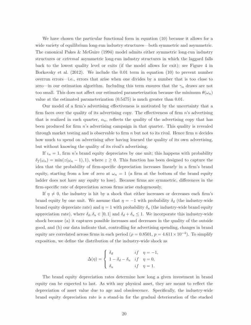
We have chosen the particular functional form in equation (10) because it allows for a

wide variety of equilibrium long-run industry structures—both symmetric and asymmetric.

The canonical Pakes & McGuire (1994) model admits either symmetric long-run industry

structures or extremal asymmetric long-run industry structures in which the laggard falls

back to the lowest quality level or exits (if the model allows for exit); see Figure 4 in

Borkovsky et al. (2012). We include the 0.01 term in equation (10) to prevent number

overrun errors—i.e., errors that arise when one divides by a number that is too close to

zero—in our estimation algorithm. Including this term ensures that the γn draws are not

too small. This does not affect our estimated parameterization because the minimum θ(ωn)

value at the estimated parameterization (0.5475) is much greater than 0.01.

Our model of a firm’s advertising effectiveness is motivated by the uncertainty that a

firm faces over the quality of its advertising copy. The effectiveness of firm n’s advertising

that is realized in each quarter, αn, reflects the quality of the advertising copy that has

been produced for firm n’s advertising campaign in that quarter. This quality is revealed

through market testing and is observable to firm n but not to its rival. Hence firm n decides

how much to spend on advertising after having learned the quality of its own advertising,

but without knowing the quality of its rival’s advertising.

If ιn = 1, firm n’s brand equity depreciates by one unit; this happens with probability

δf (ωn) = min(z(ωn − 1), 1), where z ≥ 0. This function has been designed to capture the

idea that the probability of firm-specific depreciation increases linearly in a firm’s brand

equity, starting from a low of zero at ωn = 1 (a firm at the bottom of the brand equity

ladder does not have any equity to lose). Because firms are symmetric, differences in the

firm-specific rate of depreciation across firms arise endogenously.

If η 6= 0, the industry is hit by a shock that either increases or decreases each firm’s

brand equity by one unit. We assume that η = −1 with probability δd (the industry-wide

brand equity depreciate rate) and η = 1 with probability δu (the industry-wide brand equity

appreciation rate), where δd, δu ∈ [0, 1] and δd + δu ≤ 1. We incorporate this industry-wide

shock because (a) it captures possible increases and decreases in the quality of the outside

good, and (b) our data indicate that, controlling for advertising spending, changes in brand

equity are correlated across firms in each period (ρ = 0.8501, p = 4.611×10−4). To simplify

exposition, we define the distribution of the industry-wide shock as

∆(η) =

δd if η = −1,

1− δd − δu if η = 0,

δu if η = 1.

The brand equity depreciation rates determine how long a given investment in brand

equity can be expected to last. As with any physical asset, they are meant to reflect the

depreciation of asset value due to age and obsolescence. Specifically, the industry-wide

brand equity depreciation rate is a stand-in for the gradual deterioration of the stacked

20

chips category as a whole; in our data we do observe non-stacked salty snacks taking share

away from stacked chips. The firm-specific brand equity depreciation rate captures the

more conventional notion of “goodwill depreciation”—the idea that all the underpinnings

of brand equity—awareness, familiarity, advertising-created associations—will fade from

consumers’ memories over time.

Entrants. Now suppose that firm n is a potential entrant, i.e., ωn = 0. In subperiod

2, it decides whether to enter the industry. We model entry as a transition from state

ω′n = 0 to state ω′′

n 6= 0. To guarantee the existence of a Markov-perfect equilibrium in pure

strategies, we assume that entry costs are privately observed random variables (Doraszelski

& Satterthwaite 2010). In particular, at the beginning of subperiod 2 each potential entrant

draws a random entry cost φn from a log-normal distribution F (·) with location parameter

µe and scale parameter σe. Entry costs are independently and identically distributed across

firms and periods. If the entry cost is below a threshold φn, then potential entrant n enters

the industry; otherwise it persists as a potential entrant.15 Upon entry, potential entrant n

becomes incumbent firm n and its state is the exogenously set initial brand equity ωe. We

do not incorporate exit because there are no instances of exit in our data.

Value and policy functions. Define Vn(ω, γn) to be the expected net present value of

firm n’s cash flows if the industry is currently in state ω and it has drawn effectiveness

of investment γn. Incumbent firm n’s value function is V n : {1, . . . ,M} × {0, . . . ,M} ×(0,∞) → R, and its policy function xn : {1, . . . ,M} × {0, . . . ,M} × (0,∞) → [0,∞)

specifies its advertising spending in industry state ω given that it draws an effectiveness of

advertising γn. Potential entrant n’s value function is V n : {0} × {0, . . . ,M} → R, and its

policy function ξn : {0} × {0, . . . ,M} → [0, 1] specifies the probability that it enters the

industry in state ω.16

An abridged version of the remainder of the model is presented below. A detailed version

is presented is in the appendix.

Bellman equation and optimality conditions. We first present the problem that

incumbent firm n faces in subperiod 1. Incumbent firm n’s value function V n : {1, . . . ,M}×{0, . . . ,M} × (0,∞) → R is implicitly defined by the Bellman equation

Vn(ω, γn) = maxxn>0

−xn+E[

πn(ω′)|ω, xn, x−n(ω, γ−n), γn

]

+βE[

Wn(ω′)|ω, xn, x−n(ω, γ−n), γn

]

,

(11)

15 This decision rule can be represented either with the cutoff entry cost φn or with the probabilityξn ∈ [0, 1] that firm n enters the industry in state ω, for there is a one-to-one mapping between the two viaξn =

∫1(φn ≤ φn)dF (φn) = F (φn), where 1(·) is the indicator function.

16While we define value and policy functions (as well as brand value in definition (13)) as if n = 1, theanalogous functions for firm 2 (n = 2) are defined similarly.

21

where β ∈ (0, 1) is the discount factor. The second and third terms on the right-hand side

of equation (11) are firm n’s expected profit and its discounted continuation value. Solving

the optimization problem on the right-hand side of equation (11), we derive the optimality

condition for incumbent firm n’s ad spending xn(ω, γn) in industry state ω conditional on

drawing an effectiveness of advertising γn; see equation (21) in the appendix.

Suppose next that firm n is a potential entrant, i.e., ωn = 0. The value function

V n : {0} × {0, . . . ,M} × (0,∞) → R reflects the expected net present value of firm n’s

future cash flows in industry state ω′ in subperiod 2 after the firm has drawn its entry cost

φn. It is implicitly defined by the Bellman equation

Vn(ω′, φn) = max{−φn + Un(ω

e|ω′), Un(0|ω′)}, (12)

where

Un(ωn|ω′) = β[1(ω′−n = 0)[ξ−n(ω

′)Vn(ωn, ωe) + (1− ξ−n(ω

′))Vn(ωn, 0)]

+1(ω′−n > 0)Vn(ωn, ω

′−n)]

for ω′ ∈ {0} × {0, . . . ,M} and ωn ∈ {0, ωe} is the expected net present value of all future

cash flows to incumbent firm n when it is in industry state ω′ at the beginning of subperiod

2 and it transitions to brand equity state ωn during subperiod 2. Solving the optimization

problem on the right-hand side of equation (12) and integrating over φn, we derive the

optimality condition for potential entrant n’s probability of entry ξn(ω′) in industry state

ω′; see equation (25) in the appendix.

Equilibrium. We restrict attention to symmetric Markov perfect equilibria in pure strate-

gies. Existence is guaranteed by an extension of the proof in Doraszelski & Satterthwaite

(2010). Because we solve for a symmetric equilibrium, it suffices to determine the value

and policy functions of one firm, which we refer to as firm n. Solving for an equilibrium

for a particular parameterization of the model amounts to finding a value function V n(·)and policy functions ξn(·) and xn(·) that satisfy the Bellman equations and the optimality

conditions for firm n.

Because of the dependence on the random advertising effectiveness γn (see equation

11), it would be both challenging and computationally burdensome to solve this system.

We therefore integrate out γn and solve for an incumbent firm’s expected value Vn(ω) and

its expected advertising spending xn(ω)—instead of its value Vn(ω, γn) and its advertising

spending xn(ω, γn). When we integrate out γn, the terms representing the probability of

successful advertising in the Bellman equation are replaced by the expected probability of

successful advertising, which we denote ρn(ω).

Because of the functional form of our advertising response function and the distributional

assumption we make for γn, we are able to derive analytic closed-form expressions for

22

expected advertising spending xn(ω) and the expected probability of successful advertising

ρn(ω). These closed forms completely eliminate the need for numerical integration, which

would otherwise greatly increase the computational burden of equilibrium computation and

model estimation.

5.2 Estimating the dynamic model

We use maximum likelihood estimation to estimate the dynamic model, choosing parame-

ters to maximize the likelihood of observed advertising spending, entry, and state-to-state

transitions in the data.17 Some parameters are not estimable, and these we fix at values

that seem reasonable given the empirical setting. One such parameter is the entry cost.

While we account for the entry decision in the likelihood function, we are unable to estimate

the parameters of the distribution from which those entry costs are drawn because only one

instance of entry is observed in the 12 quarters in which Pringles was a monopolist. We set

these parameters to values that yield equilibrium entry probabilities in the region of 8% on

a quarterly basis: µe = 9 and σe = 2. We are also unable to identify the discount factor

β, so we set β = 0.99, which corresponds to an annual interest rate of 4.1%. We fix the

parameter k in the advertising response function to k = 10; again, this serves to ensure that

the model admits “small” values of the advertising effectiveness shock αn = eγn−k. Finally,

we set an entrant’s initial brand equity state to ωe = 16, which corresponds to STAX’s

estimated brand equity during its first active quarter, the fourth quarter of 2003.

The key methodological innovation in our dynamic framework is that it allows for varia-

tions in advertising spending (in a given industry state ω, across time) in a way that makes

both equilibrium computation and model estimation tractable. Previous papers employing

the Pakes & McGuire (1994) quality ladder model assumed that a firm’s investment pol-

icy function maps industry states into unique investment levels.18 By contrast, we assume

that in a given industry state, different levels of advertising spending may arise over time

because there are private random shocks to the effectiveness of advertising. This allows us

to rationalize the variation observed in our data—in particular, there are several industry

states that are visited multiple times and the firms make different advertising spending

decisions at different times. As a result, unlike earlier empirical papers that employed the

Pakes & McGuire (1994) quality ladder model (Gowrisankaran & Town 1997, Goettler &

Gordon 2011), we are able to apply maximum likelihood estimation because the proba-

bility density function of advertising spending in each industry state is not degenerate.

Maximum likelihood estimation is useful because it is statistically more efficient than a

simulated minimum-distance estimator such as the one used in Hall & Rust (2003) and

17Schmidt-Dengler (2006), Igami (2015), and Takahashi (2015), also estimate dynamic games using afull-solution method.

18See Gowrisankaran & Town (1997), Laincz (2005), Doraszelski & Markovich (2007), Borkovsky, Do-raszelski & Kryukov (2010), Goettler & Gordon (2011), Narajabad & Watson (2011), Borkovsky et al.(2012), Goettler & Gordon (2014), and Borkovsky (2015).

23

Goettler & Gordon (2011).

Incorporating private random shocks to advertising effectiveness does, however, present

a major challenge. Integrating over the random shocks yields two expectations: expected ad-

vertising spending and expected advertising success probability. Our model is still tractable,

however, because our modeling assumptions allow us to derive closed-form expressions for

these expectations, as shown in the appendix. An alternative approach would be to compute

these expectations using numerical methods such as Monte Carlo or recursive quadrature.

However, this would significantly increase computational burden because one must compute

these expectations many times in order to compute an equilibrium.19

Our approach to estimating the dynamic model is described in detail in the appendix.

We provide the derivation of the values of the ad effectiveness shock γn that rationalize the

observed advertising spending decisions. We then construct the likelihood function. Finally,

we explain how we estimate the model using Mathematical Programming with Equilibrium

Constraints (MPEC) (Su & Judd 2012).

5.3 Estimated parameters

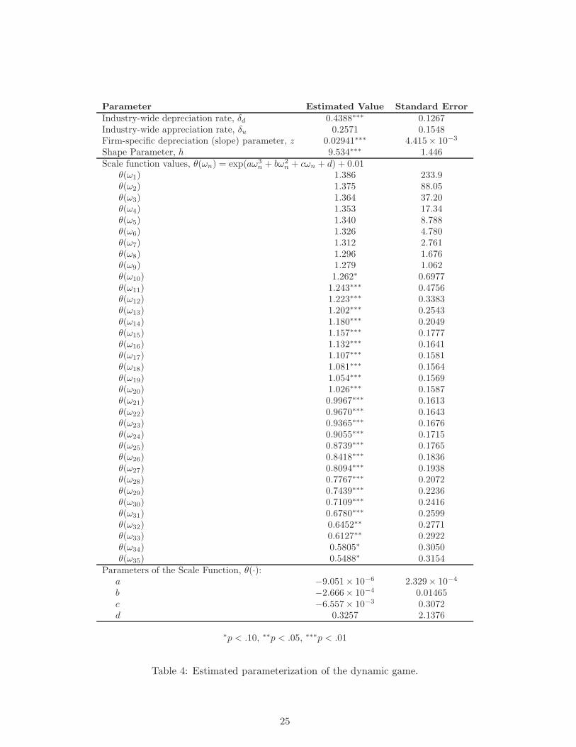
Our estimation yields the parameter estimates in Table 4 and an equilibrium of the model

that is presented in Figure 6. We calculate standard errors using a parametric bootstrap

with 100 bootstrap samples.20 The estimated parameters are sensible, though it is easier to

understand their meaning in the context of the estimated equilibrium, which is discussed in

subsection 7.2. Both industry-wide and firm-specific brand equity depreciation parameters

are statistically significant. The industry-wide appreciation rate is not statistically signif-

icant, but it is large enough (and the standard error is small enough) that we believe it

is useful to keep appreciation in the model. We find that the scale function (10) is highly

significant in the brand equity states that are spanned by the data (11, . . . , 25), which sug-

gests that advertising is effective. Because we lack data on other states, we need to rely on

our functional form assumption. The parameters of the scale function are not individually

statistically significant due to correlation between the estimated values of the parameters

of the polynomial function in equation (10). Testing the scale values themselves serves to

19For example, to compute an equilibrium at the estimated parameterization, these expectations werecomputed 1,397,656 times using our closed-form expressions.

20To accurately calculate standard errors for the dynamic model, we need to account for the estimationerror in our brand equity estimates. To do so, we sample brand equities from the estimated distributions(see Table 2) 100 times. For each sample of brand equities, we create a new discretization as in equation(8), compute the expected profit function (as in the bottom-right panel of Figure 3), and re-estimate ourdynamic model. The most burdensome part of this process is computing the expected profit function, asthis entails re-solving the static pricing game for each industry state many times (once for each pair of c andζ that are drawn). Furthermore, this must be done separately for each of the 100 samples of brand equitiesbecause, as explained above, each gives rise to a different discretization. To make this process more efficient,we do not resample the price coefficient κ, the nested parameter σ, or the standard deviation σζ of themean-zero firm-store-specific shock ζjn because the standard errors for these parameters are small relativeto their estimated values. This approach allows us to use the same Monte Carlo samples and correspondingequilibrium price calculations as in the initial expected profit function calculation via an importance sampler.

24

Parameter Estimated Value Standard Error

Industry-wide depreciation rate, δd 0.4388∗∗∗ 0.1267Industry-wide appreciation rate, δu 0.2571 0.1548Firm-specific depreciation (slope) parameter, z 0.02941∗∗∗ 4.415× 10−3

Shape Parameter, h 9.534∗∗∗ 1.446Scale function values, θ(ωn) = exp(aω3

n + bω2n + cωn + d) + 0.01

θ(ω1) 1.386 233.9θ(ω2) 1.375 88.05θ(ω3) 1.364 37.20θ(ω4) 1.353 17.34θ(ω5) 1.340 8.788θ(ω6) 1.326 4.780θ(ω7) 1.312 2.761θ(ω8) 1.296 1.676θ(ω9) 1.279 1.062θ(ω10) 1.262∗ 0.6977θ(ω11) 1.243∗∗∗ 0.4756θ(ω12) 1.223∗∗∗ 0.3383θ(ω13) 1.202∗∗∗ 0.2543θ(ω14) 1.180∗∗∗ 0.2049θ(ω15) 1.157∗∗∗ 0.1777θ(ω16) 1.132∗∗∗ 0.1641θ(ω17) 1.107∗∗∗ 0.1581θ(ω18) 1.081∗∗∗ 0.1564θ(ω19) 1.054∗∗∗ 0.1569θ(ω20) 1.026∗∗∗ 0.1587θ(ω21) 0.9967∗∗∗ 0.1613θ(ω22) 0.9670∗∗∗ 0.1643θ(ω23) 0.9365∗∗∗ 0.1676θ(ω24) 0.9055∗∗∗ 0.1715θ(ω25) 0.8739∗∗∗ 0.1765θ(ω26) 0.8418∗∗∗ 0.1836θ(ω27) 0.8094∗∗∗ 0.1938θ(ω28) 0.7767∗∗∗ 0.2072θ(ω29) 0.7439∗∗∗ 0.2236θ(ω30) 0.7109∗∗∗ 0.2416θ(ω31) 0.6780∗∗∗ 0.2599θ(ω32) 0.6452∗∗ 0.2771θ(ω33) 0.6127∗∗ 0.2922θ(ω34) 0.5805∗ 0.3050θ(ω35) 0.5488∗ 0.3154

Parameters of the Scale Function, θ(·):a −9.051× 10−6 2.329× 10−4

b −2.666× 10−4 0.01465c −6.557× 10−3 0.3072d 0.3257 2.1376

∗p < .10, ∗∗p < .05, ∗∗∗p < .01

Table 4: Estimated parameterization of the dynamic game.

25

demonstrate that the combination of these parameters, which yields the scale values, is

statistically significant.

6 Brand value estimates

As noted earlier, brand value is the expected net present value of all future cash flows

that can be attributed to the brand. In other words, from the perspective of firm n in a

given industry state ω = (ωn, ω−n), it is the difference between two firm values, Vn(ω) and

Vn(1, ω−n), the former in the actual industry state ω and the latter in the counterfactual

industry state (1, ω−n), where firm n has been stripped of its brand equity. In other words,21

υn (ω) ≡ Vn(ω)− Vn(1, ω−n). (13)

Because an equilibrium of the dynamic model includes a value function Vn(·), mapping

industry states to firm values, the factual and counterfactual firm values needed to compute

brand value are readily available once an equilibrium has been computed. Note as well that

brand building and rebuilding decisions are already folded into this mapping. For instance,

Vn(1, ω−n) already reflects the fact that firm n, being at a brand equity disadvantage in

the counterfactual situation, might try to rebuild its brand equity, and that its competitor

might strive to maintain its brand equity advantage. The resulting advertising decisions

affect subsequent brand equities, which in turn affect prices, advertising decisions, and

market structures that arise in the short- and the long-run.

In Figure 4 we show how a firm’s brand value varies as a function of its own brand

equity and that of its rival. As can be seen, a brand’s value increases relatively rapidly

in its own brand equity and decreases relatively slowly in its rival’s brand equity. These

properties arise directly from the period profit function presented in Figure 3, which shows

similar properties. Our estimates suggest that the maximum discounted cash flow potential

of a stacked chips brand is $3.36 billion, which arises when it has the highest possible brand

equity and its rival possesses the lowest possible brand equity (industry state (35, 1)). We

believe the estimated values are reasonable. As a benchmark, Pringles (worldwide, including

two production facilities) was sold for $2.7 billion in 2012, which is comparable to our

estimate of the value of the Pringles brand in the United States of $1.6 billion in 2006.

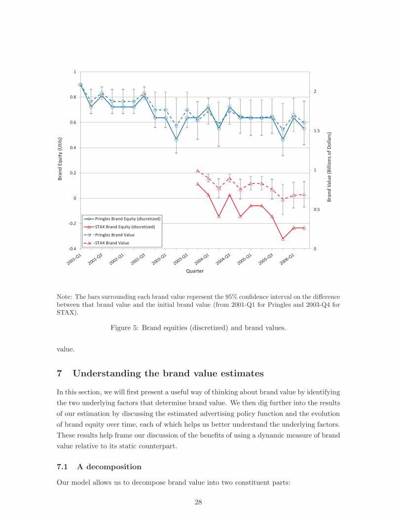
Figure 5 juxtaposes the (discretized) brand equities for Pringles and STAX against the

brand values those equities generate. Brand equity standard errors are small and were

shown earlier in Table 2. The figure includes a measure of the 95% confidence bands which

requires some explanation. While the standard errors for the brand value measures are

large— for example $463.8 million on the $2.08 billion estimate of Pringles’s brand value in

the first quarter of 2001— the measures of the changes in brand value are not. Because this

21Because firms are symmetric, the value of firm 1’s brand in industry state ω is equal to the value of firm2’s brand when the equities are reversed, i.e., υ1 (ω1, ω2) = υ2 (ω2, ω1).

26

05

1015

2025

3035

05

1015

2025

3035

0

0.5

1

1.5

2

2.5

3

3.5

ω1

ω2

υ 1(ω)

(Bill

ions

of D

olla

rs)

Figure 4: Brand values (in billions of dollars).

figure highlights how changes in brand equity and brand value differ, we display confidence

intervals which, fixing the initial level of brand value, represent the uncertainty on the

change in brand value over time. When interpreting the confidence interval in other parts

of the paper, our estimates can be seen as representing a very wide brand value range that

shifts the narrower range shown in Figure 5.22

Comparing brand equity and brand value changes shows, first, that a given change in

brand equity tends to result in a less than proportional change in the corresponding brand

value (we explain why in subsection 7.3). Second, because brand value is a function of

both own brand equity and rival brand equity, a firm’s brand value can change even if its

brand equity does not. For example, while Pringles has the same brand equity in the third

and fourth quarters of 2003, its brand value is much higher in the former ($1.77 billion)

than in the latter ($1.63 billion). The reason is clear: in the earlier quarter Pringles was a

monopolist, but in the latter quarter it faced competition from STAX. Brand value, being a

cash flow-based measure, reflects the changing productivity of brand equity under different

market conditions, while brand equity, being a consumer-based measure, does not. The

strength of competition is a key driver of the relationship between brand equity and brand

22The intuition for the difference between the standard error of the brand value and the change is brandvalue is that the brand value measures are comparisons of the equilibrium value function in two quite differentindustry states (factual and counterfactual), whereas the change in brand value compares nearby industrystates, as the counterfactuals get differenced out. The comparison of nearby states is more precise than thecomparison of distant states, and so the standard errors are smaller.

27

0

0.5

1

1.5

2

-0.4

-0.2

0

0.2

0.4

0.6

0.8

1

Bra

nd

Va

lue

(B

illi

on

s o

f D

oll

ars

)

Bra

nd

Eq

uit

y (

Uti

ls)

Quarter

Pringles Brand Equity (discretized)

STAX Brand Equity (discretized)

Pringles Brand Value

STAX Brand Value

Note: The bars surrounding each brand value represent the 95% confidence interval on the differencebetween that brand value and the initial brand value (from 2001-Q1 for Pringles and 2003-Q4 forSTAX).

Figure 5: Brand equities (discretized) and brand values.

value.

7 Understanding the brand value estimates

In this section, we will first present a useful way of thinking about brand value by identifying

the two underlying factors that determine brand value. We then dig further into the results

of our estimation by discussing the estimated advertising policy function and the evolution

of brand equity over time, each of which helps us better understand the underlying factors.

These results help frame our discussion of the benefits of using a dynamic measure of brand

value relative to its static counterpart.

7.1 A decomposition

Our model allows us to decompose brand value into two constituent parts:

28

1. The difference between factual and counterfactual flow profits over time (i.e., the profit

premium).

2. The difference between factual and counterfactual advertising expenditures over time.

As explained above, brand value in a given industry state is the difference between firm

value in the factual scenario—in which a firm possesses its brand equity—and firm value

in the counterfactual scenario, in which the firm has been stripped of its brand equity.

Because firm value in a given industry state ω is the expected net present value of all

future cash flows—where a firm’s cash flow in a given period is its period profit minus its

ad spending—we can restate firm n’s brand value in industry state ω as

υn (ω) = Vn(ω)− Vn(1, ω−n)

=

∞∑

q=0

βqE[

πn(ωq′)− xn(ω

q)|ω0 = ω]

−∞∑

q=0

βqE[

πn(ωq′)− xn(ω

q)|ω0 = (1, ω−n)]

=

∞∑

q=0

βq{(

E[

πn(ωq′)|ω0 = ω

]

− E[

πn(ωq′)|ω0 = (1, ω−n)

])

(14)

−(

E[

xn(ωq)|ω0 = ω

]

− E[

xn(ωq)|ω0 = (1, ω−n)

])}

,

where the expectation is taken over industry state ωq that arises at the beginning of quarter

q and industry state ωq′ that arises in quarter q at the end of subperiod 1, given the initial

industry state ω0.

As can be seen from this equation, brand value is the discounted present value of the

difference between factual and counterfactual expected flow profits (first row of expression

14) minus the difference between factual and counterfactual advertising expenditures (sec-

ond row of expression 14). This decomposition shows that our measure of brand value is

even more comprehensive than the profit-premium measures that are commonly viewed as

state of the art (see, e.g., Fischer 2007, Goldfarb et al. 2009). What this underscores is that

a proper accounting of brand value must necessarily recognize that a brand has an impact

not only on a firm’s flow profits, but also on its ad spending decisions. Moreover, it must

account for how the different ad spending decisions made with and without the brand cause

brand equity to evolve over time.

7.2 Brand building incentives

The decomposition presented above shows that a key determinant of brand value is the

difference between factual and counterfactual advertising expenditures. To understand this

difference, we must understand how brand equity affects a firm’s ad spending decisions. In

order to do that, let us examine Figure 6. Here the top panels show the estimated policy

29

0 5 10 15 20 25 30 350

0.03

0.06

0.09

0.12

0.15

ω2

ξ 1(ω2)

010

2030

0

10

20

30

0

0.2

0.4

0.6

0.8

1

ω1

ω2

ρ 1(ω)

0 5 10 15 20 25 30 355

6

7

8

9

10

11

12

13

14

ω1

hθ(ω

1)

010

2030

0

10

20

30

0

5

10

15

ω1

ω2

x 1(ω)

Figure 6: Estimated equilibrium: expected ad spending (in millions of dollars) (top left);probability of entry (top right); advertising success probability (bottom left); and expectedad effectiveness (bottom right).

30

functions for ad spending and the probability of entry and the bottom panels show the

advertising success probability and expected advertising effectiveness.23

The upper-left panel of Figure 6 shows that there is a non-monotonic relationship be-

tween a firm’s own brand equity and its ad spending. An increase in a firm’s brand equity

gives rise to an increase in its ad spending, but only up to brand equity ωn = 30, after which

ad spending decreases. The increase in ad spending is driven by three factors. First, as

brand equity increases, a firm spends more on advertising in order to counteract the decreas-

ing effectiveness of its advertising (measured by hθ(ωn)), which is shown in the lower-right

panel of Figure 6. Second, as brand equity increases, a firm spends more on advertising

to counteract the increasing firm-specific brand equity depreciation rate. Finally, because

the estimated period profit function is convex in a firm’s own brand equity (see Figure 3),

the higher a firm’s brand equity, the greater the returns it earns (at least in the short-run)

from further increasing its brand equity and, accordingly, the greater its incentive to in-

vest in advertising. Thus, as a firm’s brand equity increases, changes in ad effectiveness,

depreciation, and the profits that brand equity delivers all lead the firm to increase its ad

spending.

Things change, however, for ωn > 30 because at such high levels of brand equity, a

firm’s ad effectiveness is very low and its firm-specific depreciation rate is very high. It

becomes much more difficult to build and sustain brand equity and this weakens advertising

incentives. Thus when a firm has high brand equity, it usually—but not always—spends

more on advertising. Going forward, this insight will play a key role in helping us understand

the value of the Pringles and STAX brands.

7.3 Brand equity over time

The value of a brand is based on the difference between the cash flows it generates in the

factual scenario, in which it possesses its brand equity, and the counterfactual scenario,

in which it is stripped of its brand equity. Hence, to understand brand value we need

to understand how brand equity evolves over time in each of these scenarios. Section 7.2

explored how firms behave in equilibrium. Given this understanding, we can now infer how

brand equity evolves over time.

Here we focus on the industry state that arises in the last period of our data, (21,12).

The left panel of Figure 7 shows how Pringles and STAX expected brand equities evolve

over time in the factual scenario, which starts at (21,12), and in the Pringles counterfactual

scenario, which starts at (1,12).24 The x and o markers indicate the expected brand equities

in quarters 0, 10, . . . , 140 for the factual and counterfactual scenarios respectively. Pringles’s

23We include the entry policy function for completeness but do not discuss it in detail below. As noted insubsection 5.2, the entry cost parameters are not estimated because entry occurs only once in the data.

24Firm n’s expected brand equity in quarter q is Eq(ωn) =∑

ω∈{1,...,M}2 ωn × µq(ω|ω), where n = 1denotes Pringles, n = 2 denotes STAX, and the transient distribution over the set of industry states forquarters q = 1, . . . , 140, given initial industry state ω is denoted µq(ω|ω).

31

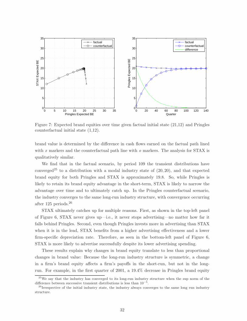
0 5 10 15 20 25 30 350

5

10

15

20

25

30

35

Pringles Expected BE

ST

AX

Exp

ecte

d B

E

factualcounterfactual

0 20 40 60 80 100 120 1400

5

10

15

20

25

30

35

Quarter

Prin

gles

Exp

ecte

d B

E

factualcounterfactualdifference

Figure 7: Expected brand equities over time given factual initial state (21,12) and Pringlescounterfactual initial state (1,12).

brand value is determined by the difference in cash flows earned on the factual path lined

with x markers and the counterfactual path line with o markers. The analysis for STAX is

qualitatively similar.

We find that in the factual scenario, by period 109 the transient distributions have

converged25 to a distribution with a modal industry state of (20, 20), and that expected

brand equity for both Pringles and STAX is approximately 19.8. So, while Pringles is

likely to retain its brand equity advantage in the short-term, STAX is likely to narrow the

advantage over time and to ultimately catch up. In the Pringles counterfactual scenario,

the industry converges to the same long-run industry structure, with convergence occurring

after 125 periods.26

STAX ultimately catches up for multiple reasons. First, as shown in the top-left panel

of Figure 6, STAX never gives up—i.e., it never stops advertising—no matter how far it

falls behind Pringles. Second, even though Pringles invests more in advertising than STAX

when it is in the lead, STAX benefits from a higher advertising effectiveness and a lower

firm-specific depreciation rate. Therefore, as seen in the bottom-left panel of Figure 6,

STAX is more likely to advertise successfully despite its lower advertising spending.

These results explain why changes in brand equity translate to less than proportional

changes in brand value: Because the long-run industry structure is symmetric, a change

in a firm’s brand equity affects a firm’s payoffs in the short-run, but not in the long-

run. For example, in the first quarter of 2001, a 19.4% decrease in Pringles brand equity

25We say that the industry has converged to its long-run industry structure when the sup norm of thedifference between successive transient distributions is less than 10−5.

26Irrespective of the initial industry state, the industry always converges to the same long run industrystructure.

32

brings about only a 10.2% decrease in its brand value; while this decline in brand equity

decreases Pringles’s profits in the short-run, it does not change the fact that the industry

will ultimately evolve to a symmetric long-run industry structure with a modal industry

state of (20, 20).

This symmetric long-run industry structure is not assumed by the model, but rather

what we conclude from our data. The dynamic model presented in Section 5 admits a wide

variety of long-run industry structures, both symmetric—where firms are likely to have the

same brand equity levels—and asymmetric—where one firm is likely to have a persistent

brand equity advantage. However, all of the equilibria presented in the paper, in this

section and below, give rise to symmetric long-run industry structures (though different

parameterizations give rise to different symmetric industry structures). The symmetric

industry structure is driven by high estimated variance of the effectiveness of advertising

(hθ(ωn)2) at low brand equity (ωn) states. This means that firms with low brand equity

never completely give up and ultimately catch up to a leader through a sequence of lucky

(though anticipated) draws.27

Because the industry converges to a symmetric long-run industry structure, the value of

a brand is derived strictly from the higher cash flows that accrue to the firm in the factual

scenario—as compared to the counterfactual scenario—before the factual and counterfac-

tual industry structures converge. For industry state (21,12), the factual scenario and the

Pringles counterfactual scenario converge after 125 quarters; thereafter Pringles’s cash flows

in the factual scenario are no higher than its cash flows in the counterfactual scenario. The

value of the Pringles brand in industry state (21,12) is therefore derived from the higher

cash flows that the firm earns in the factual scenario in the first 124 quarters. The longer

it takes for the factual and counterfactual industry structures to converge, the greater the

brand’s opportunity to create value for the firm from the additional cash flows it generates.

Our model also helps us understand the drivers of brand value. Consider Pringles’s

brand value of $1.60 billion in industry state (21,12). Using the profit function (Figure

3), the advertising policy function (Figure 6), and the transient distributions described

above (summarized in Figure 7), we can compute the two components of the brand value

decomposition presented in subsection 7.1. We find that in the factual scenario, Pringles

earns $1.79 billion in additional flow profits (the first component), but that it spends $191.3

million in additional advertising expenditures. Hence, Pringles’s brand value derives from

the fact that it earns much greater flow profits in the factual scenario, which more than

overrides its greater advertising expenditures in that scenario.

27We do not run counterfactuals on the variance of the effectiveness of advertising because we find suchcounterfactuals hard to motivate. Such counterfactuals do give rise to asymmetric long-run industry struc-tures at certain values for the variance of the effectiveness of advertising.

33

7.4 The benefits of a dynamic measure of brand value

As explained above, our measure of brand value is the dynamic counterpart of the Goldfarb

et al. (2009) purely static approach. However, there is no denying that the static measure

is easier to compute, so it is important to see what is being gained by taking an explicitly

dynamic approach.

A firm’s “static” brand value in industry state ω = (ωn, ω−n) is π∗n(ω) − π∗n(1, ω−n),

which can be computed using the equilibrium profit function that is presented in the bottom-

right panel of Figure 3. To convert this to a measure of brand value for all future periods—so

that it is comparable to our net present value measure—one can simply regard the brand as a

perpetuity that generates cash flow π∗n(ω)−π∗n(1, ω−n) in all future periods and compute the

present discounted value using the discount rate from the dynamic model. This is analogous

to abstracting from the dynamics of brand building and assuming that the industry state

does not change over time. Hence, we define

νsn(ω) =1

1− β(π∗n(ω)− π∗n(1, ω−n)), (15)

which we hereafter denote as “static brand value” for the sake of simplicity.

Figure 8 juxtaposes the “dynamic” brand values for Pringles and STAX—already pre-

sented in Figure 5—against the static brand values, and reveals dramatic differences between

the two. Specifically, the static brand values are much higher and fluctuate much more over

time.

To understand why static brand values are much higher, it is useful to refer to the

two components of the brand value decomposition in subsection 7.1. First, because the

static measure omits advertising, it does not capture the impact of the brand on a firm’s

advertising expenditures. Our dynamic brand value measure accounts for the fact that a

firm spends more on advertising in the factual scenario than the counterfactual scenario.

For example, Pringles spends $11.6 million on advertising in industry state (21,12) and only

$2.3 million in the corresponding counterfactual industry state (1,12).

Second, while the static measure captures the profit premium that the brand generates

in one period and assumes that it will continue to do so in perpetuity, the dynamic measure

accounts for the fact that a profit premium exists only until the factual and counterfactual

scenarios converge. For example, in industry state (21,12)—which prevails in the second

quarter of 2006—the static and dynamic brand values for Pringles are $7.62 billion and

$1.60 billion. Whereas the static measure implicitly assumes that the 21 units of brand

equity that Pringles possesses in the factual scenario will generate additional profits of

$76.2 million per quarter indefinitely, the dynamic measure correctly recognizes that the

incremental profits generated by the brand will decrease over time as the industry converges

to the same symmetric long-run industry structure in both the factual and counterfactual

scenarios. For example, the additional profits earned in the factual scenario decline to $50.1

34

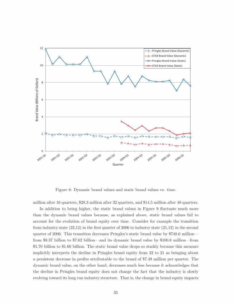
0

2

4

6

8

10

12

Bra

nd

Va

lue

(B

illi

on

s o

f D

oll

ars

)

Quarter

Pringles Brand Value (Dynamic)

STAX Brand Value (Dynamic)

Pringles Brand Value (Static)

STAX Brand Value (Static)

Figure 8: Dynamic brand values and static brand values vs. time.

million after 16 quarters, $28.3 million after 32 quarters, and $14.5 million after 48 quarters.

In addition to being higher, the static brand values in Figure 9 fluctuate much more

than the dynamic brand values because, as explained above, static brand values fail to

account for the evolution of brand equity over time. Consider for example the transition

from industry state (22,12) in the first quarter of 2006 to industry state (21,12) in the second

quarter of 2006. This transition decreases Pringles’s static brand value by $748.6 million—

from $8.37 billion to $7.62 billion—and its dynamic brand value by $100.8 million—from

$1.70 billion to $1.60 billion. The static brand value drops so starkly because this measure

implicitly interprets the decline in Pringles brand equity from 22 to 21 as bringing about

a persistent decrease in profits attributable to the brand of $7.49 million per quarter. The

dynamic brand value, on the other hand, decreases much less because it acknowledges that

the decline in Pringles brand equity does not change the fact that the industry is slowly

evolving toward its long run industry structure. That is, the change in brand equity impacts

35

the path along which the industry is traveling, but not its destination.

We have shown that because the static measure fails to account for how the profit pre-

mium evolves over time and ignores the impact of the brand on advertising expenditures, it

can produce misleading measures of brand value. This is also true of other static measures,

such as a revenue premium. For Pringles and STAX, the static measure grossly overesti-

mates brand values, and also gives rise to drastic intertemporal fluctuations that are not

reflective of the true values of these brands. These limitations will limit the usefulness of

such measures for accounting, legal, and brand strategy purposes.

8 How brand equity depreciation and advertising effective-

ness affect brand value

Our model has three key parameters that affect the ability of firms to build and sustain

brand equity: (i) the firm-specific brand equity depreciation rate, (ii) the industry-wide

brand equity depreciation rate, and (iii) the mean effectiveness of advertising. Here we

examine how changes in these parameters affect brand value, focusing primarily on the

latter two (the results for the firm-specific depreciation rate are quite similar to those for

the industry-wide depreciation rate). We focus on the industry state observed in the final

period of our data set, (21,12). Hence we explore how changes in the industry-wide brand

equity depreciation rate and advertising effectiveness affect firm value for Pringles and

STAX in industry state (21, 12) relative to industry state (1, 12) for Pringles and (21, 1) for

STAX.

8.1 Changes in the industry-wide brand equity depreciation rate

To explore the consequences of changes in the industry-wide brand equity depreciation

rate δd, we compute equilibria for δd ∈ {0, 0.05, . . . , 1}.28 As we vary the industry-wide

depreciation rate δd, we assume that the ratio of the industry-wide appreciation rate (δu)

to the probability that there is no industry-wide shock (1− δd − δu) is fixed at the ratio of

the estimated values29, i.e.,

Pr(η = 1)

Pr(η = 0)=

δu

1− δd − δu=

0.2571

0.3040= 0.8458.

All other parameters are held fixed at the estimated values.

28We compute counterfactual equilibria using a Gauss-Jacobi algorithm that is similar to the Pakes &McGuire (1994) algorithm in that it incorporates iterated best-reply and value function iteration, but itdoes so using the closed-form expressions (appendix equations 29 and 30) and the expected value function(appendix equation 33). As detailed in the appendix, we have not found any instances of multiplicity.

29By computing equilibria for all (δd, δu) pairs that satisfy the restriction δd + δu ≤ 1, we have verifiedthat our results are robust to this assumption about how δu varies as we vary δd.

36

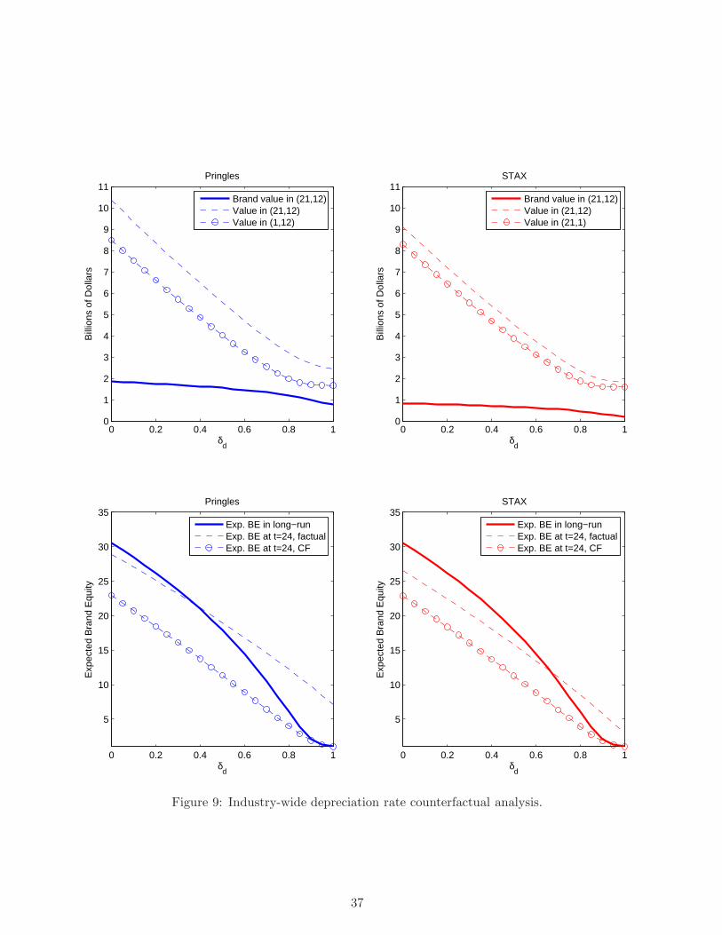
0 0.2 0.4 0.6 0.8 10

1

2

3

4

5

6

7

8

9

10

11

δd

Bill

ions

of D

olla

rs

Pringles

Brand value in (21,12)Value in (21,12)Value in (1,12)

0 0.2 0.4 0.6 0.8 10

1

2

3

4

5

6

7

8

9

10

11

δd

Bill

ions

of D

olla

rs

STAX

Brand value in (21,12)Value in (21,12)Value in (21,1)

0 0.2 0.4 0.6 0.8 1

5

10

15

20

25

30

35

δd

Exp

ecte

d B

rand

Equ

ity

Pringles

Exp. BE in long−runExp. BE at t=24, factualExp. BE at t=24, CF

0 0.2 0.4 0.6 0.8 1

5

10

15

20

25

30

35

δd

Exp

ecte

d B

rand

Equ

ity

STAX

Exp. BE in long−runExp. BE at t=24, factualExp. BE at t=24, CF

Figure 9: Industry-wide depreciation rate counterfactual analysis.

37

Firm versus brand value. Our first observation is that a given change in the industry-

wide brand equity depreciation rate has a much greater impact on firm value than on

brand value. As shown in the upper panels of Figure 9, firm value in both the factual and

counterfactual scenarios declines rapidly as the industry-wide depreciation rate increases,

but brand value declines much more slowly. For instance, increasing δd from 0 to 1 de-

creases Pringles’s firm value by $7.9 billion in the factual scenario and by $6.8 billion in the

counterfactual scenario. This rapid decline in firm value occurs because, as shown in the

bottom-left panel of Figure 9, an increase in the industry-wide depreciation rate decreases

a firm’s expected brand equity both in the short-run (after 24 quarters) and the long-run.

Therefore, at a higher industry-wide depreciation rate, a firm traverses a less profitable

path toward the long-run industry structure and earns less profit once the industry reaches

its long-run industry structure. By contrast, brand value is much less sensitive to changes

in the industry-wide depreciation rate. Increasing δd from 0 to 1 decreases Pringles brand

value by only $1.1 billion—from $1.9 billion to $763 million. Results for STAX are similar.

Intuitively, an increase in the industry-wide depreciation rate has a relatively small impact

on brand value because it has a similarly detrimental impact on firm value in both the

factual and counterfactual scenarios.

While the brand equity that a firm possesses is valuable regardless of circumstances, the

source of a brand’s value does depend on the circumstances. This is shown in the lower

panels of Figure 9. When δd = 0, the 21 units of brand equity that Pringles possesses

in the factual scenario are highly valuable because they give Pringles a big head-start in

its journey toward its expected long-run brand equity of 30.6. On the other hand, when

δd = 1, despite being unable to sustain any brand equity whatsoever, the 21 units of brand

equity that Pringles possesses in the factual scenario are still valuable because Pringles is

able to harvest them and in doing so earn significant profits even as they erode. In the

counterfactual scenario for δd = 1, Pringles earns relatively little profit because it starts

with no brand equity and it fails to build any. The sources of STAX’s brand value are

analogous, though smaller because its initial brand equity is lower.

Explaining the decrease in brand value. Figure 10 helps us understand why brand

value is decreasing in the industry-wide depreciation rate by examining the impact of the

industry-wide depreciation rate on (i) the time required for factual and counterfactual indus-

try structures to converge, and (ii) the two components of the brand value decomposition.

We restrict attention to Pringles, but the results for STAX are qualitatively similar.

We explained above that the value of a brand is derived strictly from the higher cash

flows that the firm earns in the factual scenario—relative to the counterfactual scenario—

before the factual and counterfactual industry structures converge. We first explore whether

an increase in the industry-wide depreciation rate decreases brand value because of its im-

pact on the time required for the factual and counterfactual scenarios to converge. The first

two rows of Figure 10 present the evolution of the expected industry state and Pringles’s

38

0 10 20 300

10

20

30

Pringles expected BE

ST

AX

exp

ecte

d B

E

δd=0.1

0 10 20 300

10

20

30

Pringles expected BE

ST

AX

exp

ecte

d B

E

δd=0.5

0 10 20 300

10

20

30

Pringles expected BE

ST

AX

exp

ecte

d B

E

δd=0.9

factualcounterfactual

0 20 40 60 80 1000

10

20

30

Quarter

Exp

ecte

d B

E

0 20 40 60 80 1000

10

20

30

Quarter

Exp

ecte

d B

E

0 20 40 60 80 1000

10

20

30

Quarter

Exp

ecte

d B

E

factualcounterfactualdifference

0 20 40 60 80 1000

20

40

60

80

100

Quarter

Exp

ecte

d P

rofit

s

0 20 40 60 80 1000

20

40

60

80

100

Quarter

Exp

ecte

d P

rofit

s

0 20 40 60 80 1000

20

40

60

80

100

Quarter

Exp

ecte

d P

rofit

s

0 20 40 60 80 1000

5

10

15

Quarter

Exp

ecte

d A

d S

pend

0 20 40 60 80 1000

5

10

15

Quarter

Exp

ecte

d A

d S

pend

0 20 40 60 80 1000

5

10

15

Quarter

Exp

ecte

d A

d S

pend

0 20 40 60 80 1000

20

40

60

80

100

Quarter

Exp

ecte

d C

ash

Flo

ws

0 20 40 60 80 1000

20

40

60

80

100

Quarter

Exp

ecte

d C

ash

Flo

ws

0 20 40 60 80 1000

20

40

60

80

100

Quarter

Exp

ecte

d C

ash

Flo

ws

Figure 10: Industry-wide depreciation rate counterfactual analysis (Pringles).

39

expected brand equity in the factual and counterfactual scenarios for three levels of the

depreciation rate. The second row suggests that an increase in the industry-wide deprecia-

tion rate has an immaterial impact on the time required for the factual and counterfactual

industry structures to converge. While the time required for convergence does vary across

depreciation rates30, the differences have a negligible impact on brand value because at

each depreciation rate, more than 99% of Pringles’s brand value is generated in the first

100 quarters. Having ruled out this possible explanation, we turn to the two components

of the brand value decomposition.

The third row of Figure 10 shows how Pringles’s profits differ across the factual and

counterfactual scenarios—the first factor in the brand value decomposition. An increase in

the industry-wide depreciation rate decreases the difference between factual and counter-

factual profits in the sufficiently early quarters. (In later quarters, this relationship does

not necessarily hold because of the difference across depreciation rates in the time required

for factual and counterfactual industry structures to converge. However, the overall brand

value results are driven by the earlier periods because the difference between factual and

counterfactual expected brand equity is higher and the flow profits are less discounted.)

The smaller difference (between factual and counterfactual profits) for higher deprecia-

tion rates stems from the fact that an increase in the industry-wide depreciation rate leads

to a decline in Pringles’s long-run expected brand equity; see the bottom-left panel of Figure

9 and the top row of Figure 10. For δd = 0.1, 0.5, and 0.9, the expected long-run brand

equities are 28.5, 17.9, and 2.2 respectively. The difference between factual and counterfac-

tual flow profits is greater when firms are moving toward a higher long-run expected brand

equity because a firm’s period profit function is highly convex in its own brand equity (see

Figure 3).31

Consider the factual and counterfactual paths presented in the upper-left panel of Figure

10 for δd = 0.1. The factual scenario yields much greater flow profits because the industry

travels along the steep portion of the period profit function, while in the counterfactual

scenario, the industry starts on the flat portion and reaches the steep portion only much

later. Alternatively, for δd = 0.9, in both the factual and counterfactual scenarios, the

industry travels along the relatively flat portion of the period profit function. Intuitively,

because a brand delivers greater and greater period profits—at an increasing rate—as its

brand equity increases, a firm that is able to build and sustain a high level of brand equity

benefits greatly from being able to start with relatively high brand equity instead of having

to build all of its brand equity from scratch.

The fourth row of Figure 10 shows how advertising expenditures differ across the factual

30At δd = 0.1, 0.5, and 0.9, it takes 115, 128, and 195 quarters respectively for the factual and Pringlescounterfactual industry structures to converge.

31The convexity of the period profit function should not be regarded as simply an artifact of the exponentialnature of the nested logit demand system in subsection 4.2. Rather, the convexity reflects the fact that anincrease in a firm’s brand equity gives rise to both a higher equilibrium price and—despite the higher price—ahigher quantity demanded. Accordingly, this convexity arises in even much simpler quality ladder models.

40

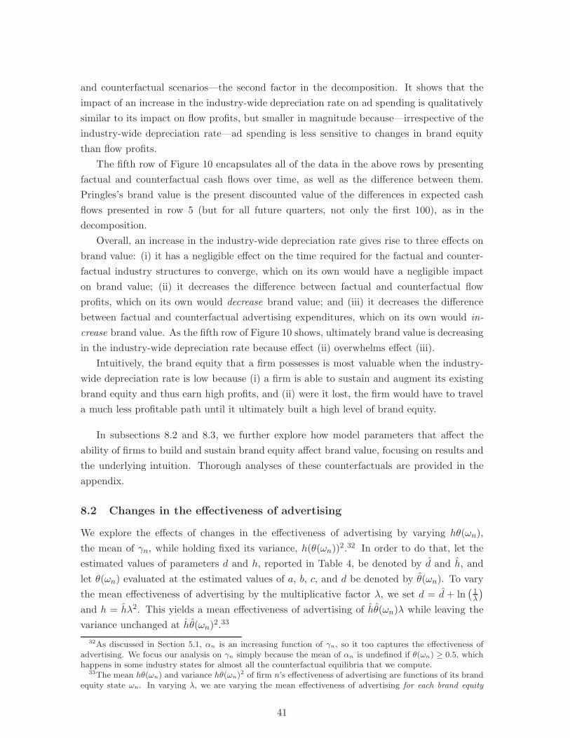
and counterfactual scenarios—the second factor in the decomposition. It shows that the

impact of an increase in the industry-wide depreciation rate on ad spending is qualitatively

similar to its impact on flow profits, but smaller in magnitude because—irrespective of the

industry-wide depreciation rate—ad spending is less sensitive to changes in brand equity

than flow profits.

The fifth row of Figure 10 encapsulates all of the data in the above rows by presenting

factual and counterfactual cash flows over time, as well as the difference between them.

Pringles’s brand value is the present discounted value of the differences in expected cash

flows presented in row 5 (but for all future quarters, not only the first 100), as in the

decomposition.

Overall, an increase in the industry-wide depreciation rate gives rise to three effects on

brand value: (i) it has a negligible effect on the time required for the factual and counter-

factual industry structures to converge, which on its own would have a negligible impact

on brand value; (ii) it decreases the difference between factual and counterfactual flow

profits, which on its own would decrease brand value; and (iii) it decreases the difference

between factual and counterfactual advertising expenditures, which on its own would in-

crease brand value. As the fifth row of Figure 10 shows, ultimately brand value is decreasing

in the industry-wide depreciation rate because effect (ii) overwhelms effect (iii).

Intuitively, the brand equity that a firm possesses is most valuable when the industry-

wide depreciation rate is low because (i) a firm is able to sustain and augment its existing

brand equity and thus earn high profits, and (ii) were it lost, the firm would have to travel

a much less profitable path until it ultimately built a high level of brand equity.

In subsections 8.2 and 8.3, we further explore how model parameters that affect the

ability of firms to build and sustain brand equity affect brand value, focusing on results and

the underlying intuition. Thorough analyses of these counterfactuals are provided in the

appendix.

8.2 Changes in the effectiveness of advertising

We explore the effects of changes in the effectiveness of advertising by varying hθ(ωn),

the mean of γn, while holding fixed its variance, h(θ(ωn))2.32 In order to do that, let the

estimated values of parameters d and h, reported in Table 4, be denoted by d and h, and

let θ(ωn) evaluated at the estimated values of a, b, c, and d be denoted by θ(ωn). To vary

the mean effectiveness of advertising by the multiplicative factor λ, we set d = d + ln(

1λ

)

and h = hλ2. This yields a mean effectiveness of advertising of hθ(ωn)λ while leaving the

variance unchanged at hθ(ωn)2.33

32As discussed in Section 5.1, αn is an increasing function of γn, so it too captures the effectiveness ofadvertising. We focus our analysis on γn simply because the mean of αn is undefined if θ(ωn) ≥ 0.5, whichhappens in some industry states for almost all the counterfactual equilibria that we compute.

33The mean hθ(ωn) and variance hθ(ωn)2 of firm n’s effectiveness of advertising are functions of its brand

equity state ωn. In varying λ, we are varying the mean effectiveness of advertising for each brand equity

41

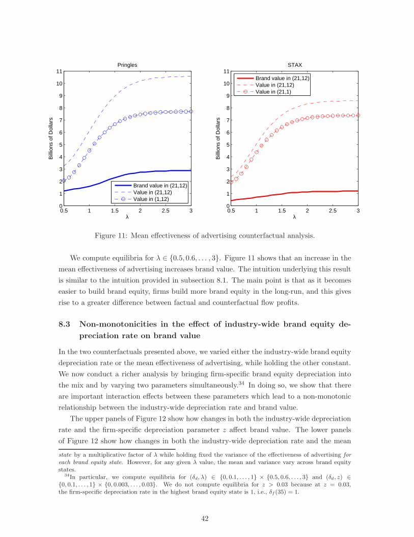
0.5 1 1.5 2 2.5 30

1

2

3

4

5

6

7

8

9

10

11

λ

Bill

ions

of D

olla

rs

Pringles

Brand value in (21,12)Value in (21,12)Value in (1,12)

0.5 1 1.5 2 2.5 30

1

2

3

4

5

6

7

8

9

10

11

λB

illio

ns o

f Dol

lars

STAX

Brand value in (21,12)Value in (21,12)Value in (21,1)

Figure 11: Mean effectiveness of advertising counterfactual analysis.

We compute equilibria for λ ∈ {0.5, 0.6, . . . , 3}. Figure 11 shows that an increase in the

mean effectiveness of advertising increases brand value. The intuition underlying this result

is similar to the intuition provided in subsection 8.1. The main point is that as it becomes

easier to build brand equity, firms build more brand equity in the long-run, and this gives

rise to a greater difference between factual and counterfactual flow profits.

8.3 Non-monotonicities in the effect of industry-wide brand equity de-

preciation rate on brand value

In the two counterfactuals presented above, we varied either the industry-wide brand equity

depreciation rate or the mean effectiveness of advertising, while holding the other constant.

We now conduct a richer analysis by bringing firm-specific brand equity depreciation into

the mix and by varying two parameters simultaneously.34 In doing so, we show that there

are important interaction effects between these parameters which lead to a non-monotonic

relationship between the industry-wide depreciation rate and brand value.

The upper panels of Figure 12 show how changes in both the industry-wide depreciation

rate and the firm-specific depreciation parameter z affect brand value. The lower panels

of Figure 12 show how changes in both the industry-wide depreciation rate and the mean

state by a multiplicative factor of λ while holding fixed the variance of the effectiveness of advertising for

each brand equity state. However, for any given λ value, the mean and variance vary across brand equitystates.

34In particular, we compute equilibria for (δd, λ) ∈ {0, 0.1, . . . , 1} × {0.5, 0.6, . . . , 3} and (δd, z) ∈{0, 0.1, . . . , 1} × {0, 0.003, . . . , 0.03}. We do not compute equilibria for z > 0.03 because at z = 0.03,the firm-specific depreciation rate in the highest brand equity state is 1, i.e., δf (35) = 1.

42

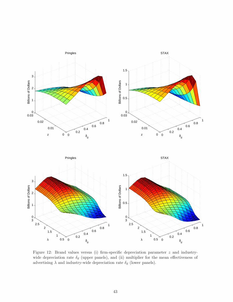
00.2

0.40.6

0.81

0.51

1.52

2.530

1

2

3

δd

Pringles

λ

Bill

ions

of D

olla

rs

00.2

0.40.6

0.81

0.51

1.52

2.530

0.5

1

1.5

δd

STAX

λ

Bill

ions

of D

olla

rs

00.2

0.40.6

0.81

0

0.01

0.02

0.030

1

2

3

δd

Pringles

z

Bill

ions

of D

olla

rs

00.2

0.40.6

0.81

0

0.01

0.02

0.030

0.5

1

1.5

δd

STAX

z

Bill

ions

of D

olla

rs

Figure 12: Brand values versus (i) firm-specific depreciation parameter z and industry-wide depreciation rate δd (upper panels), and (ii) multiplier for the mean effectiveness ofadvertising λ and industry-wide depreciation rate δd (lower panels).

43

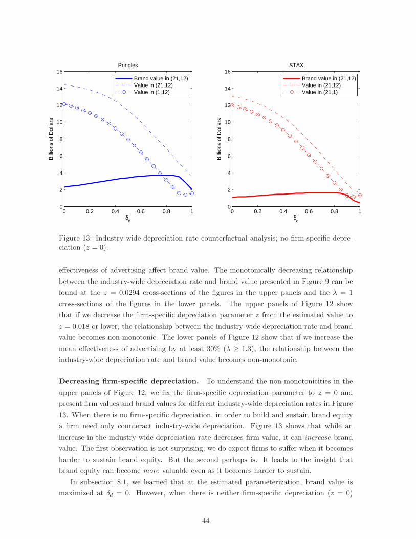
0 0.2 0.4 0.6 0.8 10

2

4

6

8

10

12

14

16

δd

Bill

ions

of D

olla

rs

Pringles

Brand value in (21,12)Value in (21,12)Value in (1,12)

0 0.2 0.4 0.6 0.8 10

2

4

6

8

10

12

14

16

δd

Bill

ions

of D

olla

rs

STAX

Brand value in (21,12)Value in (21,12)Value in (21,1)

Figure 13: Industry-wide depreciation rate counterfactual analysis; no firm-specific depre-ciation (z = 0).

effectiveness of advertising affect brand value. The monotonically decreasing relationship

between the industry-wide depreciation rate and brand value presented in Figure 9 can be

found at the z = 0.0294 cross-sections of the figures in the upper panels and the λ = 1

cross-sections of the figures in the lower panels. The upper panels of Figure 12 show

that if we decrease the firm-specific depreciation parameter z from the estimated value to

z = 0.018 or lower, the relationship between the industry-wide depreciation rate and brand

value becomes non-monotonic. The lower panels of Figure 12 show that if we increase the

mean effectiveness of advertising by at least 30% (λ ≥ 1.3), the relationship between the

industry-wide depreciation rate and brand value becomes non-monotonic.

Decreasing firm-specific depreciation. To understand the non-monotonicities in the

upper panels of Figure 12, we fix the firm-specific depreciation parameter to z = 0 and

present firm values and brand values for different industry-wide depreciation rates in Figure

13. When there is no firm-specific depreciation, in order to build and sustain brand equity

a firm need only counteract industry-wide depreciation. Figure 13 shows that while an

increase in the industry-wide depreciation rate decreases firm value, it can increase brand

value. The first observation is not surprising; we do expect firms to suffer when it becomes

harder to sustain brand equity. But the second perhaps is. It leads to the insight that

brand equity can become more valuable even as it becomes harder to sustain.

In subsection 8.1, we learned that at the estimated parameterization, brand value is

maximized at δd = 0. However, when there is neither firm-specific depreciation (z = 0)

44

nor industry-wide depreciation (δd = 0), firms can build brand equity relatively easily. It

follows that a firm in the counterfactual scenario rebuilds brand equity quickly. Hence,

the factual and counterfactual scenarios converge quickly and, accordingly, the brand has

little value. When the industry-wide depreciation rate is very high (e.g., δd = 0.95), brand

value is low because a firm is unable to sustain its brand equity, and it spends heavily on

advertising in order to slow its decline, which erodes cash flows. However, at intermediate

levels of industry-wide depreciation, brand value is high because (i) a firm is able to sustain

and enhance its brand equity and therefore generate high cash flows (relative to the coun-

terfactual scenario), and (ii) if brand equity were lost, it would be very time-consuming to

rebuild.

Increasing the mean effectiveness of advertising. The source of the non-monotonicities

in the lower panels of Figure 12 (for λ ≥ 1.3) is similar because an increase in the mean

effectiveness of advertising and a decrease in the firm-specific depreciation parameter have

similar impacts; both make it easier for firms to build and sustain brand equity. In the

appendix, we fix λ = 2 and present firm values and brand values as in Figure 13. Here we

simply emphasize the key insights. First, when ad effectiveness is sufficiently high—just as

when firm-specific depreciation is sufficiently low—while an increase in the industry-wide

depreciation rate decreases firm value, it increases brand value. Second, brand value is

highest at moderate industry-wide depreciation rates for the very same reasons described

above—i.e., the firm is able to build and sustain a high level of brand equity and, should it

be lost, the rebuilding process would be very time-consuming and much less profitable.

Summary of counterfactual analyses. The counterfactual analyses conducted in Sec-

tion 8 have generated four important insights. First, in all of the counterfactual analyses, a

change in brand building ability has a bigger impact on firm value than on brand value. Be-

cause a given change in brand building ability has a similar impact—positive or negative—on

firm value in both the factual and the counterfactual scenarios, brand value—the difference

between the two—is affected much less.

Second, in all of our counterfactual analyses, brand value is maximized under the same

set of circumstances: (i) a firm is able to build and sustain a relatively high level of brand

equity and thus earn high profits, and (ii) were the firm to lose its brand equity, the process

of rebuilding it would be very time-consuming and much less profitable.

Third, at the estimated parameterization, a change in an industry fundamental causes

brand value to vary monotonically. Therefore, the circumstances under which brand value

is maximized are at the extremes—either a very low industry-wide depreciation rate or very

high mean effectiveness of advertising. These extremal values make it possible for a firm to

achieve condition (i) because both low industry-wide depreciation and high ad effectiveness

make it easier to sustain and enhance brand equity.

Fourth, while the relationship between the industry-wide depreciation rate and brand

45

value is monotonically decreasing at the estimated parameterization, this is not necessarily

so at other parameterizations. In particular, if a change in industry fundamentals makes

it easier for a firm to sustain and enhance brand equity—e.g., a reduction in firm-specific

depreciation or an increase in ad effectiveness—then this can give rise to an inverted-U

relationship between the industry-wide depreciation rate and brand value. It follows that

brand value is highest at an intermediate industry-wide depreciation rate.

9 Conclusion

We develop a structural model of brand management to estimate the value of a brand to a

firm. Our brand value measure is forward-looking and accounts for competition within the

category, brand equity depreciation, and opportunities to build and sustain brand equity via

advertising. In our framework, a brand’s value is the expected net present value of future

cash flows accruing to a firm due to the brand. Pinning down the specific contribution of the

brand calls for a comparison between a factual scenario—in which a product possesses its

brand equity—and a hypothetical counterfactual scenario—in which the product is stripped

of its brand equity. Our structural model allows us to account for the different decisions

that consumers and firms make across these scenarios. For example, in the counterfactual

scenario, a firm is stripped of its brand equity, and this affects consumers’ purchasing

decisions and, in turn, the pricing and advertising decisions of the firm and its rival over

time.

Using data from the U.S. stacked chips category for the period 2001–2006, we provide

quarterly estimates of brand equity and brand value for the Pringles and STAX brands.

We find that a given change in brand equity gives rise to a less than proportional change

in brand value. We also compare our brand value measure to an analogous static measure

that ignores advertising and accordingly its ability to shape brand equity dynamics. The

static measure yields brand values that are grossly overestimated and that fluctuate too

much over time.

Our structural model allows us to explore how changes in a firm’s ability to build and

sustain brand equity affect the value of its brand. Perhaps most notably, we find that

when industry conditions make it easier to brand build, an increase in the industry-wide

brand equity depreciation rate can increase brand value, even as it (expectedly) reduces

firm value. So, a brand becomes more valuable even as the brand equity on which it is

constituted becomes harder to sustain.

We believe our framework breaks new ground by offering a way to measure, and under-

stand, brand value that is integrated into a dynamic model of brand management. Further-

more, we believe that our framework could be adapted to industries whose details might

differ from those of the stacked chips category, the subject of this study, and augmented

to answer other important questions on brand valuation and brand management. First,

while we study the national-level brand management decisions observed in the stacked

46

chips category, in some product categories, geographic differences in consumers’ preferences

may induce firms to manage their brands more locally (Bronnenberg, Dhar & Dube 2007).

Second, while the assumption that firms build brand equity via investments in advertis-

ing applies well to the stacked chips category in the period 2001–2006, in other product

categories, especially in more recent times, firms are building brand equity in a variety of

different ways, of which advertising is only one component. Third, while we have restricted

attention to a product category in which each firm operates a single brand, one could extend

our methods to product categories in which firms maximize profits over multiple brands.

47

References

Aaker, D. A. & Biel, A. L. (1993), Brand equity and advertising, Hillsdale, NJ.

Ailawadi, K., Lehmann, D. & Neslin, S. (2003), ‘Revenue premium as an outcome measureof brand equity’, Journal of Marketing 67, 1–17.

Ataman, B., Mela, C. & van Heerde, H. (2008), ‘Building brands’, Marketing Science

27, 1036–1054.

Bagwell, K. (2007), The economic analysis of advertising, inM. Armstrong & R. Porter, eds,‘Handbook of industrial organization’, Vol. 3, North-Holland, Amsterdam, pp. 1701–1844.

Barwise, P., Higson, C., & Likierman, A. (1989), Accounting for brands, London BusinessSchool, London, UK.

Borkovsky, R. (2015), The timing of version releases: A dynamic duopoly model, Workingpaper, University of Toronto, Toronto.

Borkovsky, R., Doraszelski, U. & Kryukov, S. (2010), ‘A user’s guide to solving dynamicstochastic games using the homotopy method’, Operations Research 58(4), 1116–1132.

Borkovsky, R., Doraszelski, U. & Kryukov, S. (2012), ‘A dynamic quality ladder duopolywith entry and exit: Exploring the equilibrium correspondence using the homotopymethod’, Quantitative Marketing and Economics 10(2), 197–229.

Bronnenberg, B., Dhar, S. & Dube, J. (2007), ‘Consumer packaged goods in the unitedstates: National brands, local branding’, Journal of Marketing Research 44, 413.

Bronnenberg, B., Kruger, M. & Mela, C. (2008), ‘The IRI academic dataset’, Marketing

Science 27, 745–748.

Byrd, R., Nocedal, J. & Waltz, R. (2006), Knitro: An integrated package for nonlinearoptimization, in G. di Pillo & M. Roma, eds, ‘Large-Scale Nonlinear Optimization’,Springer-Verlag, New York, pp. 35–59.

Caplan, J. (2008), ‘The man buried in a pringles can’, TIME .

Caplin, A. & Nalebuff, B. (1991), ‘Aggregation and imperfect competition: On the existenceof equilibrium’, Econometrica 59(1), 26–59.

Chintagunta, P. & Vilcassim, N. (1992), ‘An empirical investigation of advertising strategiesin a dynamic duopoly’, Management Science 38(9), 1230–1244.

Clark, R., Doraszelski, U. & Draganska, M. (2009), ‘The effect of advertising on brandawareness and perceived quality: An empirical investigation using panel data’, Quan-

titative Marketing and Economics 7, 207236.

de la Merced, M. (2012), ‘Kellogg to buy Procter & Gamble’s Pringles group’, New York

Times .

Dixit, A. & Pindyck, R. (1994), Investment under uncertainty, Princeton University Press,Princeton.

48

Doganoglu, T. & Klapper, D. (2006), ‘Goodwill and dynamic advertising strategies’, Quan-

titative Marketing and Economics 4(1), 5–29.

Doraszelski, U. & Markovich, S. (2007), ‘Advertising dynamics and competitive advantage’,RAND Journal of Economics 38(3), 1–36.

Doraszelski, U. & Satterthwaite, M. (2010), ‘Computable Markov-perfect industry dynam-ics’, RAND Journal of Economics 41(2), 215–243.

Dube, J., Hitsch, G. & Manchanda, P. (2005), ‘An empirical model of advertising dynamics’,Quantitative Marketing and Economics 3, 107–144.

Dube, J. & Manchanda, P. (2005), ‘Differences in dynamic brand competition across mar-kets: An empirical analysis’, Marketing Science 24(1), 81–95.

Erdem, T., Keane, M. & Sun, B. (2008), ‘A dynamic model of brand choice when price andadvertising signal product quality’, Marketing Science 27, 1111–1125.

Ericson, R. & Pakes, A. (1995), ‘Markov-perfect industry dynamics: A framework for em-pirical work’, Review of Economic Studies 62, 53–82.

Ferjani, M., Jedidi, K. & Jagpal, S. (2009), ‘A conjoint approach for consumer- and firm-level brand valuation’, Journal of Marketing Research 46, 846–862.

Fischer, M. (2007), ‘Valuing brand assets: A cost-effective and easy-to-implement measure-ment approach’, MSI Reports 7(2), 25–50.

Goettler, R. & Gordon, B. (2011), ‘Does AMD spur Intel to innovate more?’, Journal ofPolitical Economy 119(6), 1141–1200.

Goettler, R. & Gordon, B. (2014), ‘Competition and product innovation in dynamicoligopoly’, Quantitative Marketing and Economics 12(1), 1–42.

Goldfarb, A., Lu, Q. & Moorthy, S. (2009), ‘Measuring brand value in an equilibriumframework’, Marketing Science 28, 69–86.

Gowrisankaran, G. & Town, R. (1997), ‘Dynamic equilibrium in the hospital industry’,Journal of Economics and Management Strategy 6(1), 45–74.

Hall, G. & Rust, J. (2003), Simulated minimum distance estimation of a model of optimalcommodity price speculation with endogenously sampled prices, working paper, YaleUniversity, New Haven, CT.

Holbrook, M. (1992), ‘Product quality, attributes and brand name as determinants of price:The case of consumer electronics’, Marketing Letters 3, 71–83.

Horsky, D. (1977), ‘An empirical analysis of the optimal advertising policy’, Marketing

Science 23, 1037–1049.

Igami, M. (2015), ‘Estimating the innovators dilemma: Structural analysis of creative de-struction in the hard disk drive industry, 1981-1998’, Journal of Political Economy

forthcoming.

Judd, K. (1998), Numerical methods in economics, MIT Press, Cambridge.

49

Kamakura, W. & Russell, G. (1993), ‘Measuring brand value with scanner data’, Interna-tional Journal of Research in Marketing 10, 9–22.

Keller, K. (2008), Strategic brand management, 3rd ed., Prentice Hall, Upper Saddle River,NJ.

Laincz, C. (2005), ‘Market structure and endogenous productivity growth: How doR&D subsidies affect market structure?’, Journal of Economic Dynamics and Con-

trol 29, 187–223.

Narajabad, B. & Watson, R. (2011), ‘The dynamics of innovation and horizontal differen-tiation’, Journal of Economic Dynamics and Control 35(6), 825–842.

Nerlove, M. & Arrow, K. (1962), ‘Optimal advertising policy under dynamic considerations’,Economica 29(114), 129–142.

Nevo, A. (2001), ‘Measuring market power in the ready-to-eat cereal industry’, Economet-

rica 2, 307–342.

Pakes, A. & McGuire, P. (1994), ‘Computing Markov-perfect Nash equilibria: Numericalimplications of a dynamic differentiated product model’, RAND Journal of Economics

25(4), 555–589.

Rosen, S. (1974), ‘Hedonic prices and implicit markets: Product differentiation in purecompetition’, Journal of Political Economy 82, 34–55.

Rust, J. (1987), ‘Optimal replacement of GMC bus engines: An empirical model of HaroldZurcher’, Econometrica 55(5), 999–1033.

Schmidt-Dengler, P. (2006), The timing of new technology adoption: The case of MRI,Working paper, University of Vienna, Vienna.

Simon, C. & Sullivan, M. (1993), ‘The measurement and determinants of brand equity: Afinancial approach’, Marketing Science 12, 28–52.

Srinivasan, V. & Park, C. (1997), ‘Surprising robustness of the self-explicated ap-proach to customer preference structure measurement’, Journal of Marketing Research

34(2), 286–291.

Srinivasan, V., Park, C. & Chang, D. (2005), ‘An approach to the measurement, analysis,and prediction of brand equity and its sources’, Management Science 51(10), 1433–1448.

Sriram, S., & Kalwani, M. (2007), ‘Optimal advertising and promotion budgets in dynamicmarkets with brand equity as a mediating variable’, Management Science 53(1), 46–60.

Su, C. & Judd, K. (2012), ‘Constrained optimization approaches to estimation of structuralmodels’, Econometrica 80(5), 2213–2230.

Sudhir, K. (2001), ‘Competitive pricing behavior in the auto market: A structural analysis’,Marketing Science 20(1), 42–60.

50

Swait, J., Erdem, T., Louviere, J. & Dubelaar, C. (1993), ‘The equalization price: A measureof consumer-perceived brand equity’, International Journal of Research in Marketing

10(1), 23–45.

Takahashi, Y. (2015), ‘Estimating a war of attrition: The case of the U.S. movie theaterindustry’, American Economic Review 105(7), 2204–2241.

Tellis, G. J. (1988), ‘Advertising exposure, loyalty, and brand purchase: A two-stage modelof choice’, Journal of marketing research pp. 134–144.

51

A Appendix

In subsection A.1, we provide the derivation of the equilibrium conditions of the dynamic

model. In subsection A.2, we present the derivations of the closed-form expressions for

expected advertising spending and the expected probability of successful advertising. In

subsection A.3, we provide a detailed description of our approach to estimating the dynamic

model. In subsection A.4, we present the derivation of the probability distribution function

of a firm’s advertising spending in a given industry state. In subsection A.5, we provide

detailed discussions of the counterfactual analyses presented in subsections 8.2 and 8.3. In

subsection A.6, we explain how we search for multiple equilibria.

A.1 A dynamic model of brand building: Deriving the equilibrium con-

ditions

In this subsection, we present the optimization problems that the firms face and derive the

equilibrium conditions of the dynamic model. An abridged version of this material appears

in subsection 5.1, pp. 21-23.

Bellman equation and optimality conditions. We first present the problem that

incumbent firm n faces in subperiod 1. Incumbent firm n’s value function V n : {1, . . . ,M}×{0, . . . ,M} × (0,∞) → R is implicitly defined by the Bellman equation

Vn(ω, γn) = maxxn>0

−xn+E[

πn(ω′)|ω, xn, x−n(ω, γ−n), γn

]

+βE[

Wn(ω′)|ω, xn, x−n(ω, γ−n), γn

]

,

(16)

where x−n(ω, γ−n) is the rival’s advertising spending in industry state ω when it draws an

advertising effectiveness γ−n, β ∈ (0, 1) is the discount factor, and

E[

πn(ω′)|ω, xn, x−n(ω, γ−n), γn

]

=eγn−kxn

1 + eγn−kxnY 1n (ω) +

1

1 + eγn−kxnY 0n (ω) (17)

is the expected profit that incumbent firm n earns in subperiod 1 through product market

competition. Y τnn (ω) is incumbent firm n’s expected profit conditional on an investment

52

success (τn = 1) or failure (τn = 0), respectively, as given by

Y τnn (ω) =

∫

γ−n

∑

η ∈ {−1, 0, 1}ιn ∈ {0, 1}ι−n ∈ {0, 1}τ−n ∈ {0, 1}

∆(η)δf (ωn)ιn(1− δf (ωn))

1−ιnδf (ω−n)ι−n(1− δf (ω−n))

1−ι−n

×(

eγ−n−kx−n(ω, γ−n)

1 + eγ−n−kx−n(ω, γ−n)

)τ−n(

1

1 + eγ−n−kx−n(ω, γ−n)

)1−τ−n

×πn(max{min{ωn + τn − ιn + η,M}, 1},max{min{ω−n + τ−n − ι−n + η,M}, 1})×dΓ(γ−n|h, θ(ω−n)). (18)

The min and max operators merely enforce the bounds of the state space. The continuation

value in the Bellman equation (16) is

E[

Wn(ω′)|ω, xn, x−n(ω, γ−n), γn

]

=eγn−kxn

1 + eγn−kxnZ1n(ω) +

1

1 + eγn−kxnZ0n(ω). (19)

Wn(ω′), which is defined formally below, denotes the expected net present value of all future

cash flows to incumbent firm n when it is in industry state ω′ at the beginning of subperiod

2. Zτnn (ω) is the expected net present value of all future cash flows to incumbent firm n

when it is in industry state ω at the beginning of subperiod 1 conditional on an investment

success (τn = 1) or failure (τn = 0), respectively, as given by

Zτnn (ω) =

∫

γ−n

∑

η ∈ {−1, 0, 1}ιn ∈ {0, 1}ι−n ∈ {0, 1}τ−n ∈ {0, 1}

∆(η)δf (ωn)ιn(1− δf (ωn))

1−ιnδf (ω−n)ι−n(1− δf (ω−n))

1−ι−n

×(

eγ−n−kx−n(ω, γ−n)

1 + eγ−n−kx−n(ω, γ−n)

)τ−n ( 1

1 + eγ−n−kx−n(ω, γ−n)

)1−τ−n

×Wn(max{min{ωn + τn − ιn + η,M}, 1},max{min{ω−n + τ−n − ι−n + η,M}, 1})×dΓ(γ−n|h, θ(ω−n)). (20)

Solving incumbent firm n’s maximization problem in subperiod 1, we find that

xn(ω, γn) = max

{

0,−1 +

√

eγn−kTn (ω)

eγn−k

}

, (21)

where Tn (ω) ≡ Y 1n (ω) − Y 0

n (ω) + β(Z1n(ω) − Z0

n(ω)), if Tn (ω) > 0 and xn(ω, γn) = 0

otherwise.

53

While the incumbent firm does not take action in subperiod 2, it is affected by the

actions taken by a potential entrant, if one exists. It follows that the expected net present

value of all future cash flows to incumbent firm n when it is in industry state ω′ at the

beginning of subperiod 2 is

Wn(ω′) =

[

1(ω′−n > 0) + 1(ω′

−n = 0)(1 − ξ−n(ω′)]

Vn(ω′) (22)

+1(ω′−n = 0)ξ−n(ω

′)Vn(ω′n, ω

e)

for ω′ ∈ {1, . . . ,M} × {0, . . . ,M}, where

Vn(ω) =∫

γn[ − xn(ω, γn) + E [πn(ω

′)|ω, xn(ω, γn), x−n(ω, γ−n), γn]+βE [Wn(ω

′)|ω, xn(ω, γn), x−n(ω, γ−n), γn] ] dΓ(γn|h, θ(ωn)).(23)

Suppose next that firm n is a potential entrant, i.e., ωn = 0. The value function

V n : {0} × {0, . . . ,M} × (0,∞) → R reflects the expected net present value of firm n’s

future cash flows in industry state ω′ in subperiod 2 after the firm has drawn its entry cost

φn. It is implicitly defined by the Bellman equation

Vn(ω′, φn) = max{−φn + Un(ω

e|ω′), Un(0|ω′)}, (24)

where

Un(ωn|ω′) = β[1(ω′−n = 0)[ξ−n(ω

′)Vn(ωn, ωe) + (1− ξ−n(ω

′))Vn(ωn, 0)]

+1(ω′−n > 0)Vn(ωn, ω

′−n)]

for ω′ ∈ {0} × {0, . . . ,M} and ωn ∈ {0, ωe} is the expected net present value of all future

cash flows to incumbent firm n when it is in industry state ω′ at the beginning of subperiod

2 and it transitions to brand equity state ωn during subperiod 2. Letting χ(ω′, φn) be the

indicator function that takes the value of one if firm n enters and zero otherwise yields

χn(ω′, φn) = argmax

χ∈{0,1}{χ(−φn + Un(ω

e|ω′)) + (1− χ)Un(0|ω′)}.

The probability of drawing a setup cost φn such that χn(ω′, φn) = 1 determines the proba-

bility that firm n enters:

ξn(ω′) = F (Un(ω

e|ω′)− Un(0|ω′)). (25)

We can now restate the Bellman equation (24) in terms of the potential entrant’s expected

value function

Vn(ω′) =

∫

φn

Vn(ω′, φn)dF (φn),

54

which reflects the expected value in industry state ω′ at the beginning of subperiod 2, before

the setup cost has been drawn. The expected value function V n : {0} × {0, . . . ,M} → R is

implicitly defined by the Bellman equation

Vn(ω′) = ξn(ω

′){−E{φn|φn 6 F−1(ξn)}+ Un(ωe|ω′)}+ (1− ξn(ω

′))Un(0|ω′).

The relevant expected setup cost is not the unconditional expectation E(φn), but rather

the expectation of the setup cost conditional on entering

E{φn|φn ≥ F−1(ξn)} = eµe−(σe)2

Φ

(

µe+(σe)2−ln(F−1(ξn))σe

)

Φ

(

µe−ln(F−1(ξn))σe

) .

Equilibrium. We restrict attention to symmetric Markov perfect equilibria in pure strate-

gies. Existence is guaranteed by an extension of the proof in Doraszelski & Satterthwaite

(2010).35 We use ω[2] to denote the vector (ω2, ω1) obtained by interchanging firms’ states.

In a symmetric equilibrium, the advertising decision taken by firm 1 in industry state ω

when it has drawn an effectiveness of advertising of γ′ is identical to the advertising decision

taken by firm 2 in industry state ω[2] when it has drawn an effectiveness of advertising of γ′,

i.e., x1(ω, γ′) = x2(ω

[2], γ′), and similarly for the value functions. Analogously, when firm 1

is a potential entrant, the probability that it enters the industry in state ω = (0, ω2) is iden-

tical to the probability that firm 2 enters the industry in state ω[2], i.e., ξ1(ω) = ξ2(ω[2]).

It therefore suffices to determine the value and policy functions of only one firm, which we

will refer to as firm n. Solving for an equilibrium for a particular parameterization of the

model amounts to finding a value function V n(·) and policy functions ξn(·) and xn(·) thatsatisfy the Bellman equations and the optimality conditions for firm n.

This system comprises the incumbent firm’s Bellman equation

Vn(ω, γn) = −xn(ω, γn) +E[

πn(ω′)|ω, xn(ω, γn), x−n(ω, γ−n), γn

]

+βE[

Wn(ω′)|ω, xn(ω, γn), x−n(ω, γ−n), γn

]

,

and optimal advertising condition (21) for ω ∈ {1, . . . ,M} × {0, . . . ,M} and γn ∈ (0,∞);

and the potential entrant’s Bellman equation

Vn(ω) = ξn(ω){−E{φn|φn 6 F−1(ξn(ω))}+ βUωe

n (ω)}+ (1− ξn(ω))βU0n(ω)} (26)

35For any γn ∈ (0,∞), the transition function for subperiod 1 that is defined above is unique investmentchoice admissible (Doraszelski & Satterthwaite 2010). It follows that for any industry state ω, the mappingfrom firm n’s advertising effectiveness draw γn to its optimal advertising spending, xn(ω, ·), is a function.Moreover, this function is a unique best-reply to any strategy played by firm n’s rival. In subperiod 2,potential entrants play cutoff entry strategies, as in Doraszelski & Satterthwaite (2010). It follows thatthere exists a symmetric Markov perfect equilibrium in pure strategies.

55

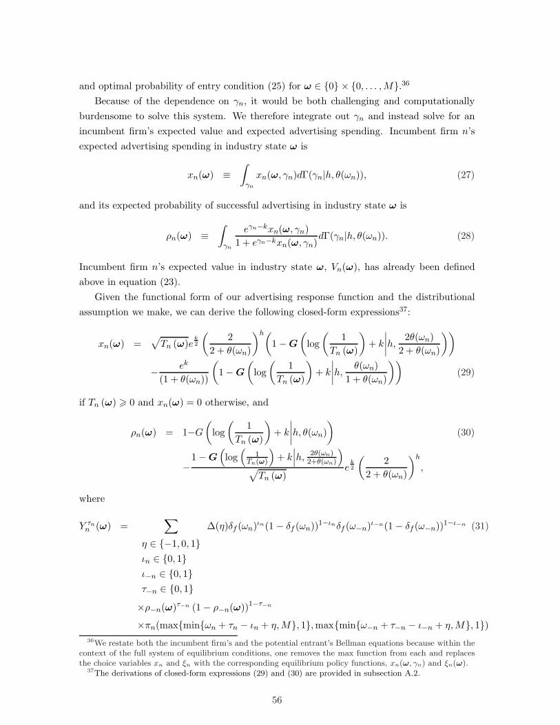
and optimal probability of entry condition (25) for ω ∈ {0} × {0, . . . ,M}.36Because of the dependence on γn, it would be both challenging and computationally

burdensome to solve this system. We therefore integrate out γn and instead solve for an

incumbent firm’s expected value and expected advertising spending. Incumbent firm n’s

expected advertising spending in industry state ω is

xn(ω) ≡∫

γn

xn(ω, γn)dΓ(γn|h, θ(ωn)), (27)

and its expected probability of successful advertising in industry state ω is

ρn(ω) ≡∫

γn

eγn−kxn(ω, γn)

1 + eγn−kxn(ω, γn)dΓ(γn|h, θ(ωn)). (28)

Incumbent firm n’s expected value in industry state ω, Vn(ω), has already been defined

above in equation (23).

Given the functional form of our advertising response function and the distributional

assumption we make, we can derive the following closed-form expressions37:

xn(ω) =√

Tn (ω)ek2

(

2

2 + θ(ωn)

)h(

1−G

(

log

(

1

Tn (ω)

)

+ k

∣

∣

∣

∣

h,2θ(ωn)

2 + θ(ωn)

))

− ek

(1 + θ(ωn))

(

1−G

(

log

(

1

Tn (ω)

)

+ k

∣

∣

∣

∣

h,θ(ωn)

1 + θ(ωn)

))

(29)

if Tn (ω) > 0 and xn(ω) = 0 otherwise, and

ρn(ω) = 1−G(

log

(

1

Tn (ω)

)

+ k

∣

∣

∣

∣

h, θ(ωn)

)

(30)

−1−G

(

log(

1Tn(ω)

)

+ k∣

∣

∣h,2θ(ωn)2+θ(ωn)

)

√

Tn (ω)e

k2

(

2

2 + θ(ωn)

)h

,

where

Y τnn (ω) =

∑

η ∈ {−1, 0, 1}ιn ∈ {0, 1}ι−n ∈ {0, 1}τ−n ∈ {0, 1}

∆(η)δf (ωn)ιn(1− δf (ωn))

1−ιnδf (ω−n)ι−n(1− δf (ω−n))

1−ι−n (31)

×ρ−n(ω)τ−n (1− ρ−n(ω))1−τ−n

×πn(max{min{ωn + τn − ιn + η,M}, 1},max{min{ω−n + τ−n − ι−n + η,M}, 1})36We restate both the incumbent firm’s and the potential entrant’s Bellman equations because within the

context of the full system of equilibrium conditions, one removes the max function from each and replacesthe choice variables xn and ξn with the corresponding equilibrium policy functions, xn(ω, γn) and ξn(ω).

37The derivations of closed-form expressions (29) and (30) are provided in subsection A.2.

56

and

Zτnn (ω) =∑

η ∈ {−1, 0, 1}ιn ∈ {0, 1}ι−n ∈ {0, 1}τ−n ∈ {0, 1}

∆(η)δf (ωn)ιn(1− δf (ωn))

1−ιnδf (ω−n)ι−n(1− δf (ω−n))

1−ι−n (32)

×ρ−n(ω)τ−n (1− ρ−n(ω))1−τ−n

×Wn(max{min{ωn + τn − ιn + η,M}, 1},max{min{ω−n + τ−n − ι−n + η,M}, 1}).

for τn ∈ {0, 1}, which enter equations (29) and (30) through Tn (ω) = Y 1n (ω) − Y 0

n (ω) +

β(Z1n(ω)− Z0

n(ω)).

We can now rewrite the system of equilibrium conditions, integrating out over γn. Be-

cause we restrict attention to symmetric equilibria, V1(ω) = V2(ω[2]), x1(ω) = x2(ω

[2]),

ρ1(ω) = ρ2(ω[2]), and ξ1(ω) = ξ2(ω

[2]); therefore, we can restrict attention to firm 1’s

problem. It follows that the vector of unknowns in equilibrium is

Φ = [ V1 (0, 0) , V1 (1, 0) , . . . , V1 (M, 0) , V1 (0, 1) , . . . , V1 (M,M) ,

ξ1 (0, 0) , . . . , ξ1 (0,M) , x1 (1, 0) , . . . , x1 (M,M) , ρ1 (1, 0) , . . . , ρ1 (M,M) ].

The system comprises

V1(ω) = −x1(ω) + E[

π1(ω′)|ω, ρ1(ω), ρ1(ω

[2])]

+ βE[

W1(ω′)|ω, ρ1(ω), ρ1(ω

[2])]

,(33)

and equations (29) and (30) for ω ∈ {1, . . . ,M} × {0, . . . ,M} and n = 1, and equations

(25) and (26) for ω ∈ {0} × {0, . . . ,M} and n = 1. Therefore, equilibria are characterized

by a system of (M + 1) (3M + 2) equations in (M + 1) (3M + 2) unknowns. In this system,

because we have integrated out over γn, equations (17) and (19) become

E[

πn(ω′)|ω, ρn(ω), ρ−n(ω)

]

= ρn(ω)Y 1n (ω) + (1− ρn(ω))Y 0

n (ω),

and

E[

Wn(ω′)|ω, ρn(ω), ρ−n(ω)

]

= ρn(ω)Z1n(ω) + (1− ρn(ω))Z0

n(ω),

respectively.

A.2 Derivations of closed-form expressions

In this subsection, we derive the closed-form expressions for firm n’s expected advertising

spending xn(ω) (equation 29) and expected probability of successful advertising ρn(ω)

(equation 30) in industry state ω.

57

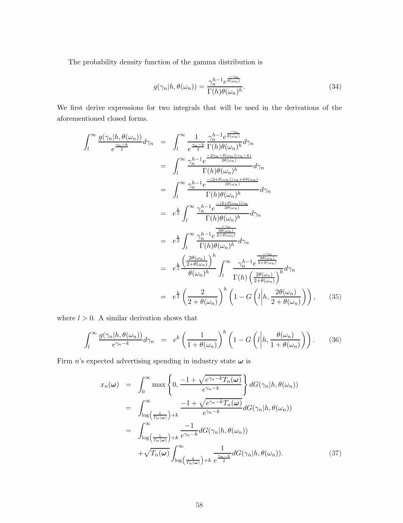
The probability density function of the gamma distribution is

g(γn|h, θ(ωn)) =γh−1n e

−γnθ(ωn)

Γ(h)θ(ωn)h. (34)

We first derive expressions for two integrals that will be used in the derivations of the

aforementioned closed forms.

∫ ∞

l

g(γn|h, θ(ωn))e

γn−k2

dγn =

∫ ∞

l

1

eγn−k

2

γh−1n e

−γnθ(ωn)

Γ(h)θ(ωn)hdγn

=

∫ ∞

l

γh−1n e

−2γn−θ(ωn)(γn−k)2θ(ωn)

Γ(h)θ(ωn)hdγn

=

∫ ∞

l

γh−1n e

−(2+θ(ωn))γn+kθ(ωn)2θ(ωn)

Γ(h)θ(ωn)hdγn

= ek2

∫ ∞

l

γh−1n e

−(2+θ(ωn))γn2θ(ωn)

Γ(h)θ(ωn)hdγn

= ek2

∫ ∞

l

γh−1n e

−γn2θ(ωn)2+θ(ωn)

Γ(h)θ(ωn)hdγn

= ek2

(

2θ(ωn)2+θ(ωn)

)h

θ(ωn)h

∫ ∞

l

γh−1n e

−γn2θ(ωn)2+θ(ωn)

Γ(h)(

2θ(ωn)2+θ(ωn)

)hdγn

= ek2

(

2

2 + θ(ωn)

)h(

1−G

(

l

∣

∣

∣

∣

h,2θ(ωn)

2 + θ(ωn)

))

, (35)

where l > 0. A similar derivation shows that

∫ ∞

l

g(γn|h, θ(ωn))eγn−k

dγn = ek(

1

1 + θ(ωn)

)h(

1−G

(

l

∣

∣

∣

∣

h,θ(ωn)

1 + θ(ωn)

))

. (36)

Firm n’s expected advertising spending in industry state ω is

xn(ω) =

∫ ∞

0max

{

0,−1 +

√

eγn−kTn(ω)

eγn−k

}

dG(γn|h, θ(ωn))

=

∫ ∞

log(

1Tn(ω)

)

+k

−1 +√

eγn−kTn(ω)

eγn−kdG(γn|h, θ(ωn))

=

∫ ∞

log(

1Tn(ω)

)

+k

−1

eγn−kdG(γn|h, θ(ωn))

+√

Tn(ω)

∫ ∞

log(

1Tn(ω)

)

+k

1

eγn−k

2

dG(γn|h, θ(ωn)). (37)

58

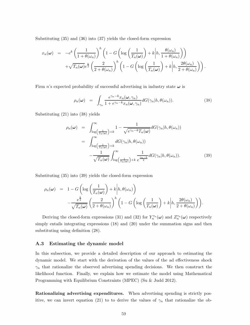
Substituting (35) and (36) into (37) yields the closed-form expression

xn(ω) = −ek(

1

1 + θ(ωn)

)h(

1−G

(

log

(

1

Tn(ω)

)

+ k

∣

∣

∣

∣

h,θ(ωn)

1 + θ(ωn)

))

+√

Tn(ω)ek2

(

2

2 + θ(ωn)

)h(

1−G

(

log

(

1

Tn(ω)

)

+ k

∣

∣

∣

∣

h,2θ(ωn)

2 + θ(ωn)

))

.

Firm n’s expected probability of successful advertising in industry state ω is

ρn(ω) =

∫

γn

eγn−kxn(ω, γn)

1 + eγn−kxn(ω, γn)dG(γn|h, θ(ωn)). (38)

Substituting (21) into (38) yields

ρn(ω) =

∫ ∞

log(

1Tn(ω)

)

+k1− 1

√

eγn−kTn(ω)dG(γn|h, θ(ωn))

=

∫ ∞

log(

1Tn(ω)

)

+kdG(γn|h, θ(ωn))

− 1√

Tn(ω)

∫ ∞

log(

1Tn(ω)

)

+k

1

eγn−k

2

dG(γn|h, θ(ωn)). (39)

Substituting (35) into (39) yields the closed-form expression

ρn(ω) = 1−G

(

log

(

1

Tn(ω)

)

+ k

∣

∣

∣

∣

h, θ(ωn)

)

− ek2

√

Tn(ω)

(

2

2 + θ(ωn)

)h(

1−G

(

log

(

1

Tn(ω)

)

+ k

∣

∣

∣

∣

h,2θ(ωn)

2 + θ(ωn)

))

.

Deriving the closed-form expressions (31) and (32) for Y τnn (ω) and Zτnn (ω) respectively

simply entails integrating expressions (18) and (20) under the summation signs and then

substituting using definition (28).

A.3 Estimating the dynamic model

In this subsection, we provide a detailed description of our approach to estimating the

dynamic model. We start with the derivation of the values of the ad effectiveness shock

γn that rationalize the observed advertising spending decisions. We then construct the

likelihood function. Finally, we explain how we estimate the model using Mathematical

Programming with Equilibrium Constraints (MPEC) (Su & Judd 2012).

Rationalizing advertising expenditures. When advertising spending is strictly pos-

itive, we can invert equation (21) to to derive the values of γn that rationalize the ob-

59

served advertising spending. Because this inversion entails solving a quadratic equation,

there are two values of γn that rationalize every positive advertising spending decision.

Let γ∗n(ωq, xqn) ≡ (γ∗n1(ωq, xqn), γ

∗n2(ωq, xqn)) be the vector of γn draws that rationalizes

observed advertising spending xqn by firm n in industry state ωq. It follows that

γ∗n(ωq, xqn) =

{

2 log

[

Tn (ωq) +√

Tn (ωq)− 4xqn

2xqn

]

+ k, (40)

2 log

[

Tn (ωq)−√

Tn (ωq)− 4xqn

2xqn

]

+ k

}

if Tn (ωq) − 4xqn ≥ 0. To understand why two different γn draws rationalize an observed

advertising spending decision, consider a firm that spends a relatively low amount on ad-

vertising. This could be rationalized by a low γn: the argument would be that with low

advertising effectiveness, it is not worthwhile spending much on advertising. However,

equally, a high αn could also justify low advertising spending: now the argument would

be that with high advertising effectiveness, even a small amount of ad spending guarantees

success.

If Tn (ωq)− 4xqn < 0, then there is no draw of γn that rationalizes observed advertising

spending xqn by firm n in industry state ωq. This is because, given any equilibrium,

there is an endogenous upper bound to advertising spending for each firm in each industry

state, namely Tn(ω)4 —the increase in expected net present value that would result if the

advertising were successful. Therefore, any advertising spending above this upper bound

has a likelihood of zero. Finally, it follows from equation (21) that given an equilibrium,

if γn < k + log(

1Tn(ω)

)

, then xn (ω) = 0. Therefore, the probability of observing zero

advertising spending by firm n in industry state ω is G(

k + log(

1Tn(ω)

)∣

∣

∣h, θ(ωn))

.

MPEC. To estimate the model, we use the MPEC approach proposed in Su & Judd

(2012). This entails maximizing the likelihood through a constrained optimization over

both the parameters and the vector of unknowns in equilibrium Φ, using the equilibrium

conditions as the set of constraints.

We take this approach for two reasons. First, we have found that MPEC produces a sig-

nificant increase in computational speed over the traditional nested fixed-point estimation

(Rust 1987). Second, in our particular problem, there are large subsets of the parame-

ter space in which the log likelihood is undefined. This occurs when observed advertising

spending exceeds the endogenous upper bound on advertising spending implied by an equi-

librium. The MPEC approach allows us to add additional constraints to ensure that the

algorithm avoids these subsets of the parameter space.

To estimate the model, we solve for the joint log likelihood of firms’ advertising spending

60

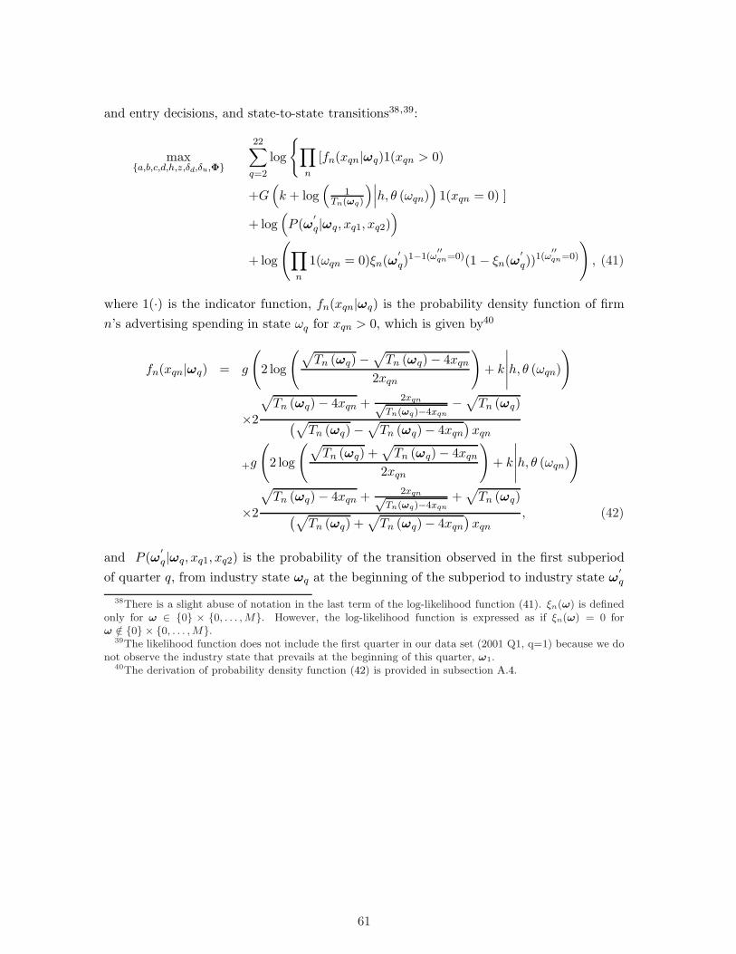
and entry decisions, and state-to-state transitions38,39:

max{a,b,c,d,h,z,δd,δu,Φ}

22∑

q=2

log

{

∏

n

[fn(xqn|ωq)1(xqn > 0)

+G(

k + log(

1Tn(ωq)

)∣

∣

∣h, θ (ωqn))

1(xqn = 0) ]

+ log(

P (ω′

q|ωq, xq1, xq2))

+ log

(

∏

n

1(ωqn = 0)ξn(ω′

q)1−1(ω

′′qn=0)(1− ξn(ω

′

q))1(ω

′′qn=0)

)

, (41)

where 1(·) is the indicator function, fn(xqn|ωq) is the probability density function of firm

n’s advertising spending in state ωq for xqn > 0, which is given by40

fn(xqn|ωq) = g

(

2 log

(

√

Tn (ωq)−√

Tn (ωq)− 4xqn

2xqn

)

+ k

∣

∣

∣

∣

∣

h, θ (ωqn)

)

×2

√

Tn (ωq)− 4xqn +2xqn√

Tn(ωq)−4xqn−√

Tn (ωq)(√

Tn (ωq)−√

Tn (ωq)− 4xqn)

xqn

+g

(

2 log

(

√

Tn (ωq) +√

Tn (ωq)− 4xqn

2xqn

)

+ k

∣

∣

∣

∣

∣

h, θ (ωqn)

)

×2

√

Tn (ωq)− 4xqn +2xqn√

Tn(ωq)−4xqn+√

Tn (ωq)(√

Tn (ωq) +√

Tn (ωq)− 4xqn)

xqn, (42)

and P (ω′

q|ωq, xq1, xq2) is the probability of the transition observed in the first subperiod

of quarter q, from industry state ωq at the beginning of the subperiod to industry state ω′

q

38There is a slight abuse of notation in the last term of the log-likelihood function (41). ξn(ω) is definedonly for ω ∈ {0} × {0, . . . ,M}. However, the log-likelihood function is expressed as if ξn(ω) = 0 forω /∈ {0} × {0, . . . ,M}.

39The likelihood function does not include the first quarter in our data set (2001 Q1, q=1) because we donot observe the industry state that prevails at the beginning of this quarter, ω1.

40The derivation of probability density function (42) is provided in subsection A.4.

61

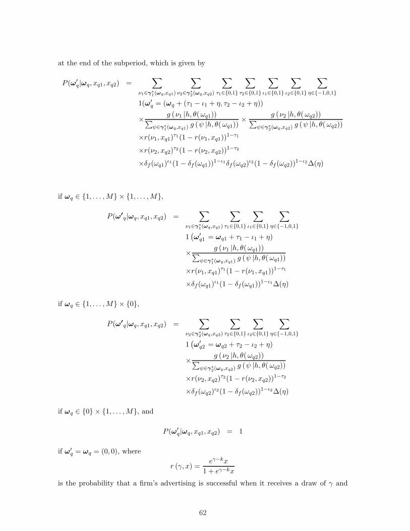
at the end of the subperiod, which is given by

P (ω′q|ωq, xq1, xq2) =

∑

ν1∈γ∗1(ωq,xq1)

∑

ν2∈γ∗2(ωq,xq2)

∑

τ1∈{0,1}

∑

τ2∈{0,1}

∑

ι1∈{0,1}

∑

ι2∈{0,1}

∑

η∈{−1,0,1}

1(ω′q = (ωq + (τ1 − ι1 + η, τ2 − ι2 + η))

× g (ν1 |h, θ(ωq1))∑

ψ∈γ∗1(ωq,xq1)

g (ψ |h, θ(ωq1))× g (ν2 |h, θ(ωq2))∑

ψ∈γ∗2(ωq ,xq2)

g (ψ |h, θ(ωq2))×r(ν1, xq1)τ1(1− r(ν1, xq1))

1−τ1

×r(ν2, xq2)τ2(1− r(ν2, xq2))1−τ2

×δf (ωq1)ι1(1− δf (ωq1))1−ι1δf (ωq2)

ι2(1− δf (ωq2))1−ι2∆(η)

if ωq ∈ {1, . . . ,M} × {1, . . . ,M},

P (ω′

q|ωq, xq1, xq2) =∑

ν1∈γ∗1(ωq,xq1)

∑

τ1∈{0,1}

∑

ι1∈{0,1}

∑

η∈{−1,0,1}

1(

ω′q1 = ωq1 + τ1 − ι1 + η)

× g (ν1 |h, θ(ωq1))∑

ψ∈γ∗1(ωq,xq1)

g (ψ |h, θ(ωq1))×r(ν1, xq1)τ1(1− r(ν1, xq1))

1−τ1

×δf (ωq1)ι1(1− δf (ωq1))1−ι1∆(η)

if ωq ∈ {1, . . . ,M} × {0},

P (ω′

q|ωq, xq1, xq2) =∑

ν2∈γ∗2(ωq,xq2)

∑

τ2∈{0,1}

∑

ι2∈{0,1}

∑

η∈{−1,0,1}

1(

ω′q2 = ωq2 + τ2 − ι2 + η)

× g (ν2 |h, θ(ωq2))∑

ψ∈γ∗2(ωq,xq2)

g (ψ |h, θ(ωq2))×r(ν2, xq2)τ2(1− r(ν2, xq2))

1−τ2

×δf (ωq2)ι2(1− δf (ωq2))1−ι2∆(η)

if ωq ∈ {0} × {1, . . . ,M}, and

P (ω′q|ωq, xq1, xq2) = 1

if ω′q = ωq = (0, 0), where

r (γ, x) =eγ−kx

1 + eγ−kx

is the probability that a firm’s advertising is successful when it receives a draw of γ and

62

spends x on advertising.41

We maximize the log-likelihood function subject to the system of equilibrium condi-

tions described at the end of subsection A.1. To these equilibrium conditions, we add the

aforementioned endogenous upper bounds on advertising spending,

xqn 6Tn(ωq)

4

for each xqn observed in the data, for the industry state ωq in which it is observed. Be-

cause these upper bounds are endogenous, adding them to the system of constraints does

not change the equilibrium set. However, it does prevent the estimation algorithm from

searching for a solution in an infeasible region. We have found that the algorithm suffers

from convergence problems if these constraints are not included.

We make the standard assumption that a single equilibrium is played in the data, and

our estimation algorithm searches for the parameterization and the equilibrium that best

rationalize the data. We have coded the maximum likelihood estimation in GAMS and run

the optimization using the KNITRO solver (Byrd, Nocedal & Waltz 2006).

A.4 Derivation of the PDF of advertising spending

This is the derivation of the probability distribution function of firm n’s strictly positive

advertising spending decisions, xn > 0, in industry state ω, fn(xn|ω). A firm does not

advertise at all in industry state ω if it draws a sufficiently low advertising effectiveness, i.e.,

γn < k+log(

1Tn(ω)

)

, which follows from equation (21). Therefore, the probability of a zero

advertising spending decision in industry state ω is simply G(

k + log(

1Tn(ω)

)∣

∣

∣h, θ(ωn))

.

In what follows, for ease of exposition, we drop the quarter subscripts, q, and we suppress

the dependence on industry state ω. To derive the PDF of firm n’s advertising spending,

we first derive its CDF. The probability that firm n’s advertising spending xn is less than

some a > 0 is:

P (xn 6 a) = P

(

−1 +√

eγ−kTn(ω)

eγ−k6 a

)

= P

(

√

eγ−kTn(ω) 6 aeγ−k + 1

)

= P

(

0 6 aeγ−k −√

eγ−kTn(ω) + 1

)

.

Notice that aeγ−k −√

eγ−kTn(ω) + 1 = 0 is a quadratic equation in the variable√eγ−k.

41Note that the realization of the depreciation shock and the outcome of advertising spending may notbe uniquely identified in each period. For example, if both firms experience a one unit decrease in brandequity, this could be caused by (i) a depreciation shock of one unit and unsuccessful advertising for bothfirms, or (ii) a depreciation shock of two units and successful advertising for both firms.

63

Solving it, we find that√eγ−k=

√Tn(ω)±

√Tn(ω)−4a

2a . It follows that

P (xn 6 a) = P

eγ−k 6

(

√

Tn(ω)−√

Tn(ω)− 4a

2a

)2

+P

eγ−k >

(

√

Tn(ω) +√

Tn(ω)− 4a

2a

)2

= G

(

2 log

(

√

Tn(ω)−√

Tn(ω)− 4a

2a

)

+ k

∣

∣

∣

∣

∣

h, θ(ωn)

)

+

(

1−G

(

2 log

(

√

Tn(ω) +√

Tn(ω)− 4a

2a

)

+ k

∣

∣

∣

∣

∣

h, θ(ωn)

)

, (43)

where G(γn|h, θ(ωn)) is the CDF of the gamma distribution from which γn is drawn.

To derive the PDF of firm n’s strictly positive advertising spending decisions, xn > 0, in

industry state ω, we take the derivative of the CDF (43) with respect to a. It follows that

fn(a|ω) = g

(

2 log

(

√

Tn(ω)−√

Tn(ω)− 4a

2a

)

+ k

∣

∣

∣

∣

∣

h, θ(ωn)

)

×2

√

Tn(ω)− 4a+ 2a√Tn(ω)−4a

−√

Tn(ω)

(√

Tn(ω)−√

Tn(ω)− 4a)a

+g

(

2 log

(

√

Tn(ω) +√

Tn(ω)− 4a

2a

)

+ k

∣

∣

∣

∣

∣

h, θ(ωn)

)

×2

√

Tn(ω)− 4a+ 2a√Tn(ω)−4a

+√

Tn(ω)

(√

Tn(ω) +√

Tn(ω)− 4a)a.

A.5 Additional details on the counterfactuals

A.5.1 Changes in the mean effectiveness of advertising

The upper panels of Figure 14 shows that an increase in the mean effectiveness of advertising

increases brand value. As before, to understand why, we need to explore the impact of this

change on the two components of the brand value decomposition, as well as the time required

for the factual and counterfactual industry structures to converge.

First, the second row of Figure 15 shows that an increase in the mean effectiveness of

advertising increases the time required for the factual and counterfactual industry structures

to converge. More effective advertising makes it easier to build and sustain brand equity.

Therefore, the higher the mean effectiveness of advertising, the greater a firm’s long-run

expected brand equity and accordingly the further a firm has to travel from both its factual

and counterfactual initial brand equity states to reach its long-run expected brand equity.42

42While an increase in the mean effectiveness of advertising does increase the rate of convergence toward

64

0.5 1 1.5 2 2.5 30

1

2

3

4

5

6

7

8

9

10

11

λ

Bill

ions

of D

olla

rs

Pringles

Brand value in (21,12)Value in (21,12)Value in (1,12)

0.5 1 1.5 2 2.5 30

1

2

3

4

5

6

7

8

9

10

11

λ

Bill

ions

of D

olla

rs

STAX

Brand value in (21,12)Value in (21,12)Value in (21,1)

0.5 1 1.5 2 2.5 3

5

10

15

20

25

30

35

λ

Exp

ecte

d B

rand

Equ

ity

Pringles

Exp. BE in long−runExp. BE at t=24, factualExp. BE at t=24, CF

0.5 1 1.5 2 2.5 3

5

10

15

20

25

30

35

λ

Exp

ecte

d B

rand

Equ

ity

STAX

Exp. BE in long−runExp. BE at t=24, factualExp. BE at t=24, CF

Figure 14: Mean effectiveness of advertising counterfactual analysis.

65

0 10 20 300

10

20

30

Pringles expected BE

ST

AX

exp

ecte

d B

E

λ=0.5

factualcounterfactual

0 10 20 300

10

20

30

Pringles expected BE

ST

AX

exp

ecte

d B

E

λ=1.3

0 10 20 300

10

20

30

Pringles expected BE

ST

AX

exp

ecte

d B

E

λ=2.1

0 20 40 60 80 1000

10

20

30

Quarter

Exp

ecte

d B

E

factualcounterfactualdifference

0 20 40 60 80 1000

10

20

30

Quarter

Exp

ecte

d B

E

0 20 40 60 80 1000

10

20

30

Quarter

Exp

ecte

d B

E

0 20 40 60 80 1000

20

40

60

80

100

Quarter

Exp

ecte

d P

rofit

s

0 20 40 60 80 1000

20

40

60

80

100

Quarter

Exp

ecte

d P

rofit

s

0 20 40 60 80 1000

20

40

60

80

100

Quarter

Exp

ecte

d P

rofit

s

0 20 40 60 80 1000

2

4

6

8

10

Quarter

Exp

ecte

d A

d S

pend

0 20 40 60 80 1000

2

4

6

8

10

Quarter

Exp

ecte

d A

d S

pend

0 20 40 60 80 1000

2

4

6

8

10

Quarter

Exp

ecte

d A

d S

pend

0 20 40 60 80 1000

20

40

60

80

100

Quarter

Exp

ecte

d C

ash

Flo

ws

0 20 40 60 80 1000

20

40

60

80

100

Quarter

Exp

ecte

d C

ash

Flo

ws

0 20 40 60 80 1000

20

40

60

80

100

Quarter

Exp

ecte

d C

ash

Flo

ws

Figure 15: Mean effectiveness of advertising counterfactual analysis (Pringles).

66

Second, the third row of Figure 15 shows that an increase in the mean effectiveness of

advertising increases the difference between factual and counterfactual flow profits. Because

an increase in ad effectiveness—like a decrease in the industry-wide depreciation rate (see

subsection 8.1)—gives rise to higher expected brand equities in the long-run, the increase

in the difference between factual and counterfactual flow profits can be attributed to the

convexity of the period profit function.

Third, the fourth row of Figure 15 shows that an increase in the mean effectiveness of

advertising has a non-monotonic effect on the difference between factual and counterfactual

advertising expenditures. That is, the difference between factual and counterfactual ad

spending is higher at intermediate levels of ad effectiveness (λ = 1.3) than at low (λ = 0.5)

or high (λ = 2.1) levels. Low ad effectiveness (λ = 0.5) weakens advertising incentives

because advertising is much less likely to succeed. High ad effectiveness (λ = 2.1) weakens

advertising incentives because advertising is likely to succeed even if the firms spends very

little on advertising. In both cases, a firm’s ad spending is relatively insensitive to its brand

equity. It follows that the difference in ad spending across the factual and counterfactual

scenarios is relatively low. On the other hand, at intermediate levels of ad effectiveness

(λ = 1.3), a firm’s ad spending is (mostly) increasing relatively rapidly in its brand equity

(as in the estimated equilibrium in Figure 6) and hence the difference between factual and

counterfactual advertising expenditures is much greater.

In summary, an increase in the mean effectiveness of advertising gives rise to three effects

on brand value: (i) it increases the time required for the factual and counterfactual industry

structures to converge, which on its own would increase brand value; (ii) it increases the

difference between factual and counterfactual flow profits, which on its own would increase

brand value; and (iii) it has a non-monotonic effect on the difference between factual and

counterfactual advertising expenditures, which on its own would have a non-monotonic

effect on brand value. The cash flows presented in the fifth row of Figure 15 show that

effects (i) and (ii) overwhelm effect (iii). Intuitively, the brand equity that a firm possesses

is most valuable when the mean effectiveness of advertising is high because (i) a firm is able

to sustain and augment its existing brand equity and thus earn high profits, and (ii) were it

lost, the process through which it rebuilt and ultimately enhanced its brand equity would

be very long and much less profitable.

A.5.2 Non-monotonic effects of the industry-wide depreciation rate on brand

value

Decreasing firm-specific depreciation. To understand the non-monotonicities in the

upper panels of Figure 12, we fix z = 0 and present results in Figures 16 and 17 that are

analogous to those presented earlier. When z = 0, the firm does not face any firm-specific

the long-run industry structure, this is moderated by the fact that the probability of successful advertisingis bounded above and therefore can only increase so much.

67

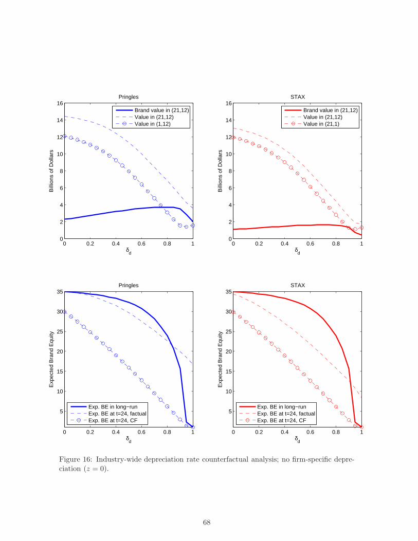
0 0.2 0.4 0.6 0.8 10

2

4

6

8

10

12

14

16

δd

Bill

ions

of D

olla

rs

Pringles

Brand value in (21,12)Value in (21,12)Value in (1,12)

0 0.2 0.4 0.6 0.8 10

2

4

6

8

10

12

14

16

δd

Bill

ions

of D

olla

rs

STAX

Brand value in (21,12)Value in (21,12)Value in (21,1)

0 0.2 0.4 0.6 0.8 1

5

10

15

20

25

30

35

δd

Exp

ecte

d B

rand

Equ

ity

Pringles

Exp. BE in long−runExp. BE at t=24, factualExp. BE at t=24, CF

0 0.2 0.4 0.6 0.8 1

5

10

15

20

25

30

35

δd

Exp

ecte

d B

rand

Equ

ity

STAX

Exp. BE in long−runExp. BE at t=24, factualExp. BE at t=24, CF

Figure 16: Industry-wide depreciation rate counterfactual analysis; no firm-specific depre-ciation (z = 0).

68

0 10 20 300

10

20

30

Pringles expected BE

ST

AX

exp

ecte

d B

E

δd=0.1

0 10 20 300

10

20

30

Pringles expected BE

ST

AX

exp

ecte

d B

E

δd=0.85

0 10 20 300

10

20

30

Pringles expected BE

ST

AX

exp

ecte

d B

E

δd=0.95

factualcounterfactual

0 20 40 60 80 1000

10

20

30

Quarter

Exp

ecte

d B

E

0 20 40 60 80 1000

10

20

30

Quarter

Exp

ecte

d B

E

0 20 40 60 80 1000

10

20

30

Quarter

Exp

ecte

d B

E

factualcounterfactualdifference

0 20 40 60 80 1000

50

100

150

Quarter

Exp

ecte

d P

rofit

s

0 20 40 60 80 1000

50

100

150

Quarter

Exp

ecte

d P

rofit

s

0 20 40 60 80 1000

50

100

150

Quarter

Exp

ecte

d P

rofit

s

0 20 40 60 80 100−10

0

10

20

Quarter

Exp

ecte

d A

d S

pend

0 20 40 60 80 100−10

0

10

20

Quarter

Exp

ecte

d A

d S

pend

0 20 40 60 80 100−10

0

10

20

Quarter

Exp

ecte

d A

d S

pend

0 20 40 60 80 1000

50

100

150

Quarter

Exp

ecte

d C

ash

Flo

ws

0 20 40 60 80 1000

50

100

150

Quarter

Exp

ecte

d C

ash

Flo

ws

0 20 40 60 80 1000

50

100

150

Quarter

Exp

ecte

d C

ash

Flo

ws

Figure 17: Industry-wide depreciation rate counterfactual analysis (Pringles); no firm-specific depreciation (z = 0).

69

depreciation; therefore to successfully build and sustain brand equity it need only counteract

industry-wide depreciation.

The upper panels of Figure 16 show that while an increase in the industry-wide depre-

ciation rate (expectedly) decreases firm value, it can perhaps surprisingly increase brand

value. That is, the brand equity that a firm possesses becomes more valuable even as it

becomes harder to sustain. To understand this relationship, as before, we must consider

the impact of this change on the two components of the brand value decomposition, as well

as the time required for the factual and counterfactual industry structures to converge.

First, the top two rows of Figure 17 show that an increase in the industry-wide depreci-

ation rate increases the time required for the factual and counterfactual industry structures

to converge. Because firms do not face firm-specific depreciation, the long-run expected

brand equities that they are able to achieve are quite high; see the lower panels of Figure

16, as compared to the lower panels of Figure 9. The higher the industry-wide depreciation

rate, the longer it takes for firms to converge to these relatively high long-run expected

brand equities, and accordingly the longer it takes for the factual and counterfactual indus-

try structures to converge. It follows that an increase in the industry-wide depreciation rate

provides the brand with greater opportunity to contribute value to the firm by increasing

the number of quarters in which it can generate excess cash flows.

Second, the third row of Figure 17 shows that—largely due to the slow convergence

described above—at high industry-wide depreciation rates, the difference between factual

and counterfactual flow profits is quite high. That being said, it does decline at δd = 0.95

because the firm is unable to build or even sustain its brand equity.

Third, the fourth row of Figure 17 shows that an increase in the industry-wide depre-

ciation rate increases the difference between factual and counterfactual advertising expen-

ditures. Notice that at very high industry-wide depreciation rates (see δd = 0.95), a firm

spends very heavily on advertising in the factual scenario as compared to the counterfac-

tual scenario. However, because a firm is unable to sustain its brand equity, the high ad

spending is undertaken strictly in order to slow its decline.

In summary, an increase in the industry-wide depreciation rate enhances brand value

primarily because it increases the time it takes for the factual and counterfactual industry

structures to converge and, in doing so, enhances the brand’s opportunity to create value

for the firm. However, at a sufficiently high industry-wide depreciation rate, the profits

that the brand contributes decline because the firm can no longer sustain its brand equity,

and the ad spending required to offset the depreciation becomes prohibitively high. These

countervailing effects gives rise to the non-monotonicities observed in the upper panels of

Figure 16.

Intuitively, when there is no firm-specific depreciation, the brand equity a firm possesses

is most valuable at an intermediate industry-wide depreciation rate (δ = .85) because (i)

a firm is able to sustain and enhance its brand equity and therefore generate high profits,

70

and (ii) were it lost, the process through which it rebuilt and ultimately enhanced its brand

equity would be very long and much less profitable.

Increasing ad effectiveness. To understand why increasing the effectiveness of adver-

tising gives rise to the non-monotonic relationship between the industry-wide depreciation

rate and brand value that is shown in the lower panels of Figure 12, we set λ = 2 and

present results in Figures 18 and 19 that are analogous to those in Figures 9 and 10. As

before, we must consider the impact of an increase in the industry-wide depreciation rate

on the two components of the brand value decomposition, as well as the time required for

the factual and counterfactual industry structures to converge.

The impact of an increase in the industry-wide depreciation rate in the face of higher

ad effectiveness (λ = 2) is mostly similar to the impact of such a change in the face of

lower firm-specific depreciation (z = 0), described above, simply because both make it

easier for a firm to build and sustain brand equity. Accordingly, Figure 19 shows that

the impact of an increase in the industry-wide depreciation rate on the time required for

convergence (second row) and on the difference between factual and counterfactual flow

profits (third row) is qualitatively similar to the effects seen in Figure 17. However, the effect

on the difference between factual and counterfactual advertising expenditures—the second

component of the decomposition—is qualitatively different: This difference is relatively

small at all parameterizations because when advertising is more effective, firms spend much

less on advertising. Therefore, this effect plays a minimal role. It follows that the intuition

as to why brand value is maximized at an intermediate industry-wide depreciation rate (δ =

0.35) is similar to that provided above for the scenario in which firm-specific depreciation

is decreased.

A.6 Multiple equilibria

Borkovsky et al. (2010) and Borkovsky et al. (2012) find that multiplicity arises in the Pakes

& McGuire (1994) quality ladder model when the equilibrium correspondence—which maps

parameterizations into equilibria—bends back on itself. This gives rise to S-shaped paths in

the equilibrium correspondence and accordingly to subsets of the parameter space in which

there are three (or more) equilibria.

We search for multiplicity in the subset of the parameter space explored in the counter-

factual analyses in Section 8 using a simple continuation method (Judd 1998, pp. 176-179)

that varies one parameter while holding all others parameter values fixed. We use the sim-

ple continuation method to compute equilibria for δd ∈ {0, 0.01, . . . , 1}, first incrementing

δd upwards—from δd = 0 to δd = 1—and then downwards—from δd = 1 to δd = 0.43 We

43If the simple continuation method were exploring a path that includes an S-shape, then it would traceout the bottom segment of the S-shape when run upwards and the top segment of the S-shaped when rundownwards. This would indicate that one must then employ another algorithm to find the equilibria on themiddle segment of the S-shape.

71

0 0.2 0.4 0.6 0.8 10

2

4

6

8

10

12

14

δd

Bill

ions

of D

olla

rs

Pringles

Brand value in (21,12)Value in (21,12)Value in (1,12)

0 0.2 0.4 0.6 0.8 10

2

4

6

8

10

12

14

δd

Bill

ions

of D

olla

rs

STAX

Brand value in (21,12)Value in (21,12)Value in (21,1)

0 0.2 0.4 0.6 0.8 1

5

10

15

20

25

30

35

δd

Exp

ecte

d B

rand

Equ

ity

Pringles

Exp. BE in long−runExp. BE at t=24, factualExp. BE at t=24, CF

0 0.2 0.4 0.6 0.8 1

5

10

15

20

25

30

35

δd

Exp

ecte

d B

rand

Equ

ity

STAX

Exp. BE in long−runExp. BE at t=24, factualExp. BE at t=24, CF

Figure 18: Industry-wide depreciation rate counterfactual analysis; increased ad effective-ness (λ = 2).

72

0 10 20 300

10

20

30

Pringles expected BE

ST

AX

exp

ecte

d B

E

δd=0.1

0 10 20 300

10

20

30

Pringles expected BE

ST

AX

exp

ecte

d B

E

δd=0.35

0 10 20 300

10

20

30

Pringles expected BE

ST

AX

exp

ecte

d B

E

δd=0.9

factualcounterfactual

0 20 40 60 80 1000

10

20

30

Quarter

Exp

ecte

d B

E

0 20 40 60 80 1000

10

20

30

Quarter

Exp

ecte

d B

E

0 20 40 60 80 1000

10

20

30

Quarter

Exp

ecte

d B

E

factualcounterfactualdifference

0 20 40 60 80 1000

50

100

150

Quarter

Exp

ecte

d P

rofit

s

0 20 40 60 80 1000

50

100

150

Quarter

Exp

ecte

d P

rofit

s

0 20 40 60 80 1000

50

100

150

Quarter

Exp

ecte

d P

rofit

s

0 20 40 60 80 1000

1

2

3

4

Quarter

Exp

ecte

d A

d S

pend

0 20 40 60 80 1000

1

2

3

4

Quarter

Exp

ecte

d A

d S

pend

0 20 40 60 80 1000

1

2

3

4

Quarter

Exp

ecte

d A

d S

pend

0 20 40 60 80 1000

50

100

150

Quarter

Exp

ecte

d C

ash

Flo

ws

0 20 40 60 80 1000

50

100

150

Quarter

Exp

ecte

d C

ash

Flo

ws

0 20 40 60 80 1000

50

100

150

Quarter

Exp

ecte

d C

ash

Flo

ws

Figure 19: Industry-wide depreciation rate counterfactual analysis (Pringles); increased adeffectiveness (λ = 2).

73

run this simple continuation method for λ ∈ {0.5, 0.6, . . . , 3} and z ∈ {0, 0.003, . . . , 0.03},holding all other parameters (except for δd) fixed at the estimated values. In doing so,

we search for multiplicity in the counterfactual results presented in Figures 9, 12, 13, 16,

and 18. The objective is to determine whether the paths plotted in these figures ever bend

back on themselves and thus give rise to multiple equilibria. To search for multiplicity in

the results presented in Figures 11 and 14, we use a simple continuation method to com-

pute equilibria for λ ∈ {0.5, 0.525, . . . , 3}, first incrementing λ upwards—from λ = 0.5 to

λ = 3—and then downwards—from λ = 3 to λ = 0.5.

We do not find any instances of multiplicity. This is of course no guarantee that the

model does not admit multiplicity. Moreover, there may be multiple equilibria that the

method described above would find at parameterizations that were not explored in the

counterfactual analyses in Section 8.

74