Investigation of a Technique for Measuring Dynamic Ground ... · Investigation of a Technique for Measuring Dynamic Ground Effect in a ... Investigation of a Technique for Measuring

NASA/CR- 1999-209544

Investigation of a Technique for

Measuring Dynamic Ground Effect in aSubsonic Wind Tunnel

Sharon S. Graves

The George Washington University

Joint Institute for Advancement of Flight Sciences

Langley Research Center, Hampton, Virginia

August 1999

https://ntrs.nasa.gov/search.jsp?R=19990081122 2018-07-02T10:38:07+00:00Z

The NASA STI Program Office ... in Profile

Since its founding, NASA has been dedicated

to the advancement of aeronautics and spacescience. The NASA Scientific and Technical

Information (STI) Program Office plays a key

part in helping NASA maintain this importantrole.

The NASA STI Program Office is operated by

Langley Research Center, the lead center forNASA's scientific and technical information.

The NASA STI Program Office provides

access to the NASA STI Database, the largest

collection of aeronautical and space scienceSTI in the world. The Program Office is alsoNASA's institutional mechanism for

disseminating the results of its research anddevelopment activities. These results are

published by NASA in the NASA STI Report

Series, which includes the following report

types:

TECHNICAL PUBLICATION. Reportsof completed research or a major

significant phase of research that

present the results of NASA programsand include extensive data or theoretical

analysis. Includes compilations of

significant scientific and technical dataand information deemed to be of

continuing reference value. NASA

counterpart and peer-reviewed formal

professional papers, but having lessstringent limitations on manuscript

length and extent of graphic

presentations.

TECHNICAL MEMORANDUM.

Scientific and technical findings that arepreliminary or of specialized interest,

e.g., quick release reports, working

papers, and bibliographies that containminimal annotation. Does not contain

extensive analysis.

CONTRACTOR REPORT. Scientific and

technical findings by NASA-sponsored

contractors and grantees.

CONFERENCE PUBLICATION.

Collected papers from scientific andtechnical conferences, symposia,

seminars, or other meetings sponsored

or co-sponsored by NASA.

SPECIAL PUBLICATION. Scientific,technical, or historical information from

NASA programs, projects, and missions,

often concerned with subjects having

substantial public interest.

TECHNICAL TRANSLATION. English-

language translations of foreignscientific and technical material

pertinent to NASA's mission.

Specialized services that complement theSTI Program Office's diverse offerings

include creating custom thesauri, building

customized databases, organizing andpublishing research results ... even

providing videos.

For more information about the NASA STI

Program Office, see the following:

• Access the NASA STI Program HomePage at http://www.stLnasa.gov

• E-mail your question via the Intemet [email protected]

• Fax your question to the NASA STI

Help Desk at (301) 621-0134

• Phone the NASA STI Help Desk at (301)621-0390

Write to:

NASA STI Help DeskNASA Center for AeroSpace Information7121 Standard Drive

Hanover, MD 21076-1320

NASA/CR- 1999-209544

Investigation of a Technique for

Measuring Dynamic Ground Effect in aSubsonic Wind Tunnel

Sharon S. Graves


Joint Institute for Advancement of Flight Sciences

Langley Research Center, Hampton, Virginia

National Aeronautics and

Space Administration

Langley Research Center

Hampton, Virginia 23681-2199

Prepared for Langley Research Center

under Cooperative Agreement NCC 1-24

August 1999

Available from:

NASA Center for AeroSpace Information (CASI)

7121 Standard Drive

Hanover, MD 21076-1320

(301) 621-0390

National Technical Information Service (NTIS)

5285 Port Royal Road

Springfield, VA 22161-2171

(703) 605-6000

Abstract

To better understand the ground effect encountered by

slender wing supersonic transport aircraft, a test was conducted

at NASA Langley Research Center's 14 x 22 foot Subsonic Wind

Tunnel in October, 1997. Emphasis was placed on improving

the accuracy of the ground effect data by using a "dynamic"

technique in which the model's vertical motion was varied

automatically during wind-on testing. This report describes and

evaluates different aspects of the dynamic method utilized for

obtaining ground effect data in this test. The method for

acquiring and processing time data from a dynamic groundeffect wind tunnel test is outlined with details of the overall data

acquisition system and software used for the data analysis. The

removal of inertial loads due to sting motion and the support

dynamics in the balance force and moment data measurements

of the aerodynamic forces on the model is described. An

evaluation of the results identifies problem areas providing

recommendations for future experiments. Test results are

validated by comparing test data for an elliptical wing planform

with an Elliptical wing planform section with a NACA 0012

airfoil to results found in current literature. Major aerodynamic

forces acting on the model in terms of lift curves for determining

ground effect are presented. Comparisons of flight and wind

tunnel data for the TU-144 are presented.

Nomenclature

Symbol Definition

A1-6

AF

AR

b

C O

C

c.g.

CL

CL ,oge

%CL

CM

F

gh

IxI

y

Izm

NF

OGE

PPM

q

Qr

RMS

SF

t

u

v

w

P

?

ti

YM

Accelerometer measurements

Axial Force, lbs

Wing model aspect ratio, b2/S

Wing model span, in

Wing model root chord, in

Wing model mean geometric chord, in

Center of gravity

Coefficient of lift in ground effect

Coefficient of lift out of ground effect

Percent increase in lift coefficient, [(CL-C_,oge)/C_,oge]X100Coefficient of pitching moment about the quarter-chord point of the mean

aerodynamic chord in ground effect

Aerodynamic force, lbs

Gravity

Height of model over ground board,

Sink rate, ft/sMoment of inertia about the x-axis

Moment of inertia about the y-axisMoment of inertia about the z-axis

Mass

Normal Force, lbs

Out of ground effect

Roll angular velocity

Pitching Moment, ft-lbs

Pitch angular velocity

dynamic pressure, psf

Yaw angular velocity

Rolling Moment, ft-lbs

Wing model area, in 2

Side Force, lbsTime

Axial velocity

Side velocity

Normal velocity

Roll angular acceleration, rad/s _

Pitch angular acceleration, rad/s _

Yaw angular acceleration, rad/s _

Axial acceleration, ft/s _

Side acceleration, ft/s 2

Normal acceleration, ft/s _

Yawing moment, ft-lbs

Angleof attack,degAL_ Leadingedgesweepangle0 Pitchangle,deg

Rollangle,degFlightpathangle(incidenceof modelpathrelativetothegroundplane,deg6 deflectionangle,deg

AcronymDGE

HSCT

HSR

MIF

MPA

OGE

TCA

Definition

Dynamic Ground EffectHigh Speed Civil Transport

High Speed ResearchModel Interface Rack

Model Preparation Area

Out of ground effect

Technical Configuration Aircraft

TABLE OF CONTENTS

NOMENCLATURE 2

TABLE OF CONTENTS 4

TABLE OF FIGURES 6

INTRODUCTION 7

EXPERIMENTAL APPROACH 9

PLANFORM 10

TABLE 1. PHYSICAL PROPERTIES OF THREE BASIC PLANFORMS.

Instrumentation

Measurement Technique

Force and Moment Data Translation

Equations for Removal of Inertial LoadsLinear Accelerations

Angular Accelerations

Velocity CalculationsSink Rate Calculation

Total Velocity Calculation

Calculated ground height, h/b

Flight Path Angle

Angle of Attack

Corrected Dynamic Pressure

Corrected Force/Moment Coefficients

Performance Coefficients

10

13

14

14

15

18

18

19

19

19

19

20

20

20

20

21

RESULTS AND DISCUSSION 22

APPENDIX A INERTIAL LOADS REMOVAL 33

APPENDIX B POST-PROCESSING DATA USING COMBOA

B.1 Logon Procedure

B.2 Setting up the Comhoa Processing Directory

52

52

52

4

B.3

B.3.1

B.4

Defining the inxxx file

rptname file

Comboa user interface

52

52

53

APPENDIX C POST PROCESSING DATA USING DYNAMIC

Input File

Output File naming convention

C.1 Setting up the Dynamic Processing Directory

Model configuration file

Model 6 configuration file



APPENDIX D ACCELEROMETERS

54

54

54

55

56

56

57

57

59

TABLE OF FIGURES

FIGURE 1. GROUND EFFECT IS ENCOUNTERED BY AN AIRPLANE

OPERATING WITHIN A SEMISPAN OF THE GROUND. 7

DIAGRAMS OF THREE RESEARCH PLANFORMS. 9

DYNAMIC GROUND EFFECT MODEL SUPPORT CART. 11

DATA ACQUISITION SYSTEM FOR DYNAMIC GROUND EFFECT

FIGURE 2.

FIGURE 3.

FIGURE 4.

TEST.

FIGURE 5.

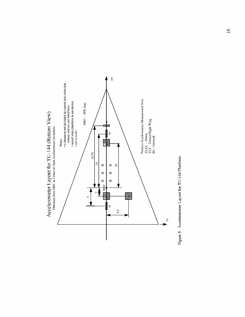
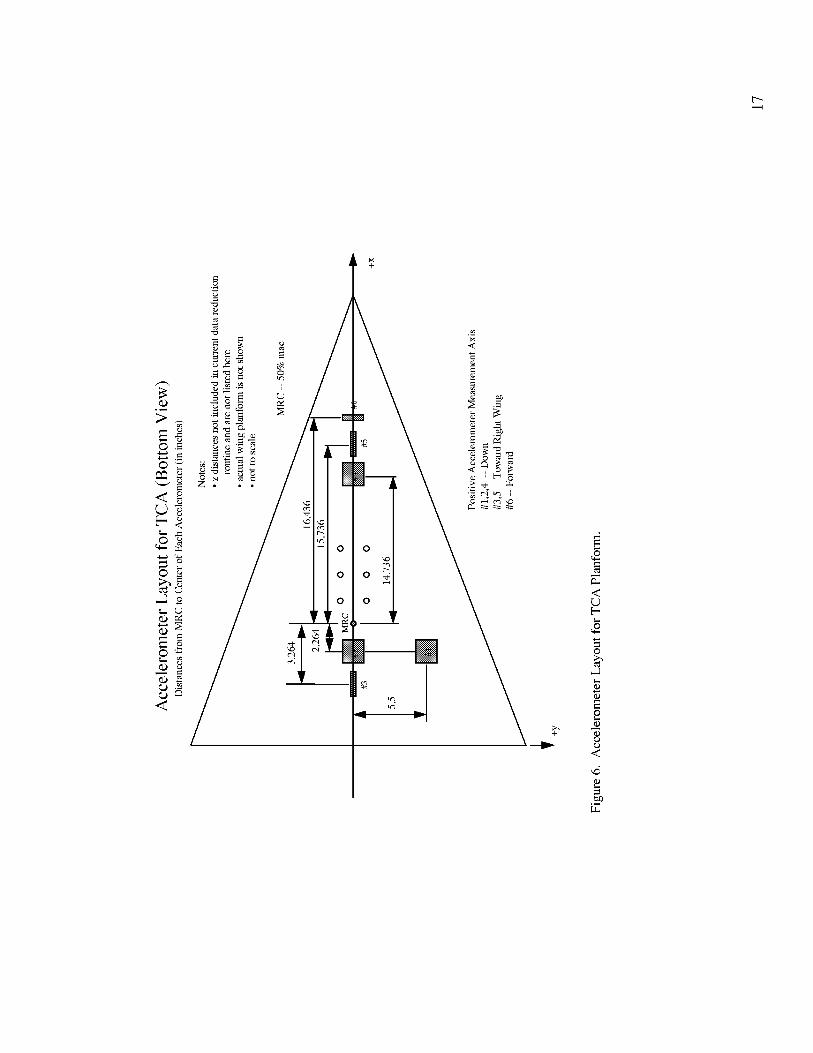
FIGURE 6.

ACCELEROMETER LAYOUT FOR TU-144 PLANFORM.

ACCELEROMETER LAYOUT FOR TCA PLANFORM.

FIGURE 7 COMPARISON OF STATIC LIFT CURVES FOR THE ELLIPTICAL

WING PLANFORM WITH THOSE IN CURRENT LITERATURE.

FIGURE 8. EFFECTS OF VARIOUS SINK RATES ON DYNAMIC GROUND

EFFECT FOR THE TU-144 PLANFORM.

FIGURE 9. EFFECTS OF VARIOUS SINK RATES ON DYNAMIC GROUND

EFFECT FOR THE TCA PLANFORM AT ALPHA = 9 DEGREES.

FIGURE 10

FIGURE 11.

EFFECT

FIGURE 12.

RATES.

FIGURE 13.

12

16

17

22

23

INERTIAL LOAD REMOVAL FOR NORMAL FORCE IN A

DYNAMIC RATE, SINK RATE = -4.667 FT/SEC. 27

FIGURE 14. SPECTRAL ANALYSIS OF DYNAMIC RUN. 28

FIGURE 15. COMPARISON OF DYNAMIC AND STATIC GROUND EFFECT LIFT

CURVES FOR TU-144 MODEL. 29


CURVES FOR TCA PLANFORM. 29


CURVES FOR ELLIPTICAL WING PLANFORM. 30

FIGURE 18. COMPARISON OF FLIGHT AND WIND TUNNEL DATA FOR TU-

144. 30

FIGURE 19. INCREMENTAL LIFT COEFFICIENT VERSUS ASPECT RATIO FOR

STATIC AND DYNAMIC GROUND EFFECT MEASURED IN THE WIND-

TUNNEL AT H/B=0.3. 31

FIGURE 20. INCREMENTAL LIFT COEFFICIENT VS ASPECT RATIO FOR

STATIC AND DYNAMIC GROUND EFFECT MEASURED IN THE WIND-

TUNNEL AT H/B =0.3. 32

25

26

24

EFFECTS OF VARIOUS SINK RATES FOR THE TU-144 PLANFORM.24

EFFECTS OF VARIOUS SINK RATES ON DYNAMIC GROUND

FOR THE ELLIPTICAL WING.

ELAPSED TIME ASSOCIATED WITH RUNS AT VARYING SINK

Introduction

The development of supersonic transport aircraft with slender wing configurations introduces

increasingly sophisticated flight control requirements for the improvement of landing and takeoff

performance. The future of the aerospace industry lies in meeting the demands for improved

performance and reliability in aircraft and doing this in less development time and at lower costs.

The conceptual and design phases play an important part in determining the airplane program

cost. 1 Correctly identifying configuration deficiencies during the preliminary design of the

aircraft can reduce both the development time and the cost of the airplane. Accurately predicting

the landing characteristics of the airplane is an important ingredient of the preliminary design

phase.

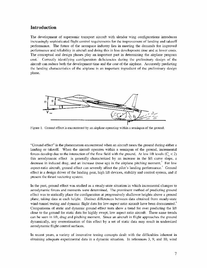
Figure 1. Ground effect is encountered by an airplane operating within a semispan of the ground.

"Ground effect" is the phenomenon encountered when an aircraft nears the ground during either a

landing or takeoff. When the aircraft operates within a semispan of the ground, incremental

forces develop due to the interaction of the flow field with the ground. At low lift levels (C L < 2)

this aerodynamic effect is generally characterized by an increase in the lift curve slope, a

decrease in induced drag, and an increase (nose up) in the airplane pitching moment. 2 For low

aspect-ratio aircraft, ground effect can severely affect the pilot's landing performance. 3 Ground

effect is a design driver of the landing gear, high lift devices, stability and control system, and if

present the thrust vectoring system.

In the past, ground effect was studied as a steady-state situation in which incremental changes to

aerodynamic forces and moments were determined. The prominent method of predicting ground

effect was to statically place the configuration at progressively shallower heights above a ground

plane, taking data at each height. Distinct differences between data obtained from steady-state

wind-tunnel testing and dynamic flight data for low-aspect ratio aircraft have been documented. 4

Comparisons of static and dynamic ground effect tests show a trend for over predicting the lift

close to the ground for static data for highly swept, low aspect ratio aircraft. These same trends

can be seen in lift, drag and pitching moment. Since an aircraft in flight approaches the ground

dynamically, any overestimation of this effect by a set of static data may result in undersized

aerodynamic flight control surfaces.

In recent years, a variety of innovative testing concepts dealt with the difficulties inherent in

obtaining adequate experimental data in a dynamic situation. In references 3, 9, and 10, wind

7

tunnel data were obtained while moving the sting-mounted model vertically to the ground plane.

Data were limited to constant rates of descent for a given run. In references 11, 14, the model

was moved horizontally through a static test chamber towards an inclined plane and data were

limited to a constant glide path angle. During typical flight landings, the portion of flight

influenced by ground effect is characterized by continuously varying sink rate and glide path

angles. Keeping conditions constant in each approach becomes more difficult as the model

approaches the ground, which coincides with the measurement period when ground effect

becomes most significant.

The measurement process is equally challenging for flight testing where flight safety becomes an

issue and the airplane must be operated within a small range of vertical and horizontal velocities

whenever it is in close proximity to the ground. In addition, flight testing is becoming

increasingly expensive and can only be performed after the aircraft has been built.

In the October 1997 Dynamic Ground Effect (DGE) Test, emphasis was placed on improving

accuracy of the ground effect data by using a "dynamic" technique in which the model's vertical

motion was varied automatically during wind-on testing. This report describes and evaluates

different aspects of the dynamic method utilized for obtaining ground effect data in this test.

Three models, the Technical Configuration Aircraft (TCA), the TU-144, and the Elliptical wing

planform with a NACA 0012 airfoil, were tested modifying external conditions incrementally.

The methodology used for acquiring and processing time data from the dynamic ground effect

wind tunnel test is described. Balance force and moment data measuring aerodynamic forces on

the model, contain significant inertial loads due to sting motion and support dynamics. Normalaccelerations were measured and used to correct these balance forces. This work addresses the

method of correction to the balance loads developed on this data.

Experimental Approach

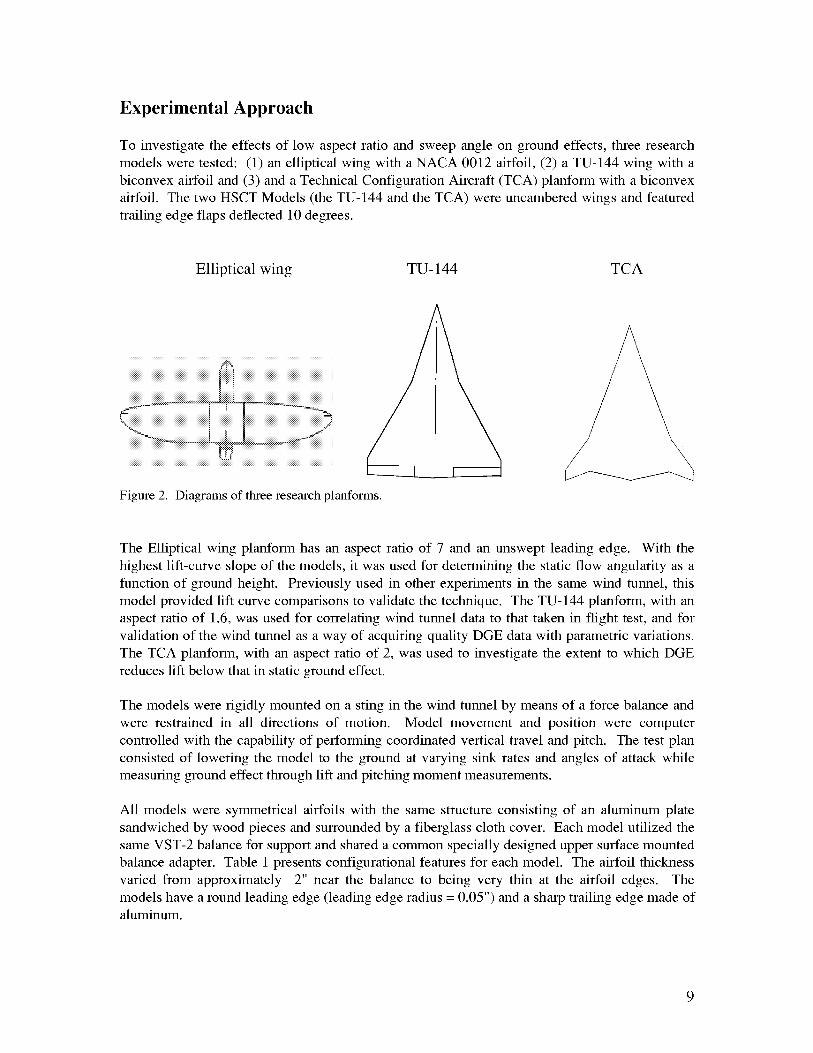
To investigate the effects of low aspect ratio and sweep angle on ground effects, three research

models were tested: (1) an elliptical wing with a NACA 0012 airfoil, (2) a TU-144 wing with a

biconvex airfoil and (3) and a Technical Configuration Aircraft (TCA) planform with a biconvex

airfoil. The two HSCT Models (the TU-144 and the TCA) were uncambered wings and featured

trailing edge flaps deflected 10 degrees.

Elliptical wing TU- 144 TCA

Figure 2. Diagrams of three research planforms.

The Elliptical wing planform has an aspect ratio of 7 and an unswept leading edge. With the

highest lift-curve slope of the models, it was used for determining the static flow angularity as a

function of ground height. Previously used in other experiments in the same wind tunnel, this

model provided lift curve comparisons to validate the technique. The TU-144 planform, with an

aspect ratio of 1.6, was used for correlating wind tunnel data to that taken in flight test, and for

validation of the wind tunnel as a way of acquiring quality DGE data with parametric variations.

The TCA planform, with an aspect ratio of 2, was used to investigate the extent to which DGE

reduces lift below that in static ground effect.

The models were rigidly mounted on a sting in the wind tunnel by means of a force balance and

were restrained in all directions of motion. Model movement and position were computer

controlled with the capability of performing coordinated vertical travel and pitch. The test plan

consisted of lowering the model to the ground at varying sink rates and angles of attack while

measuring ground effect through lift and pitching moment measurements.

All models were symmetrical airfoils with the same structure consisting of an aluminum plate

sandwiched by wood pieces and surrounded by a fiberglass cloth cover. Each model utilized the

same VST-2 balance for support and shared a common specially designed upper surface mounted

balance adapter. Table 1 presents configurational features for each model. The airfoil thickness

varied from approximately 2" near the balance to being very thin at the airfoil edges. The

models have a round leading edge (leading edge radius = 0.05") and a sharp trailing edge made ofaluminum.

Model

#

6

7

10

plan form

TCA wing

TU- 144 wing

Elliptical wing

Inbom-d

(deg)

71

outbom-d

(deg)

52

76 57

0 0

AR b (in) S Mass

(ft 2) (slgs)

2.03 48.0 7.89 1.74

1.64 47.1 9.45 1.85

7.00 80.62 6.45 4.49

Table 1. Physical properties of three basic planforms.

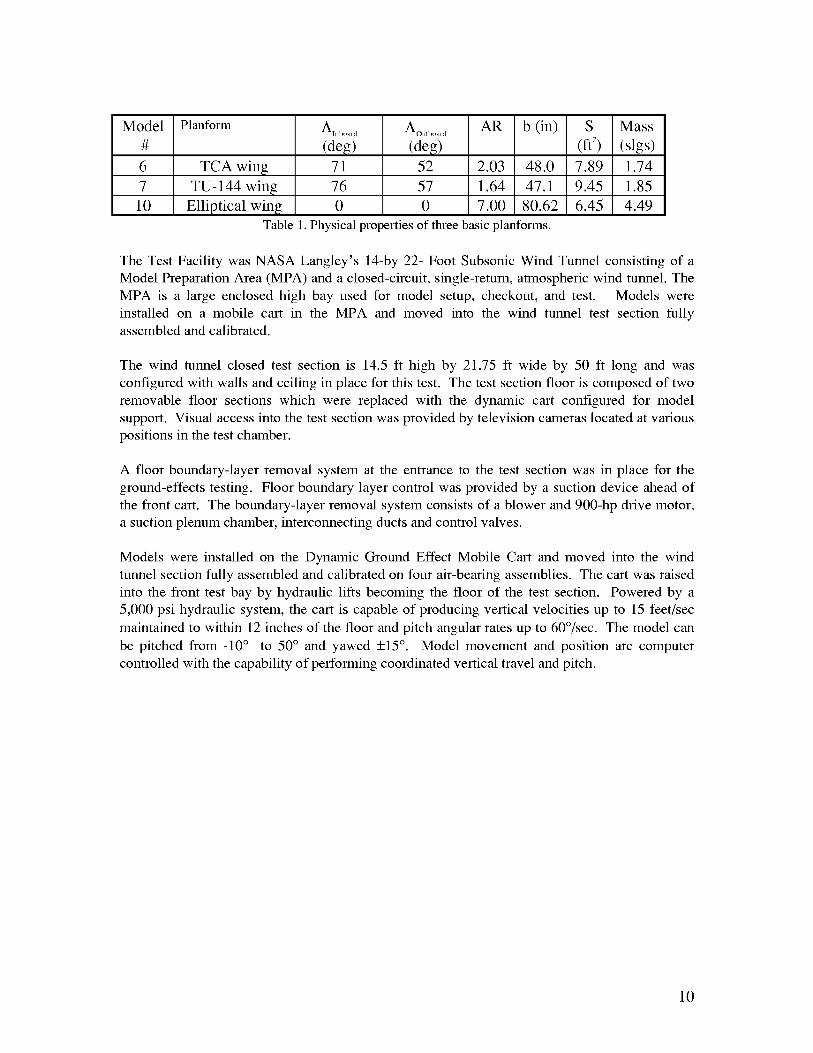
The Test Facility was NASA Langley's 14-by 22- Foot Subsonic Wind Tunnel consisting of a

Model Preparation Area (MPA) and a closed-circuit, single-return, atmospheric wind tunnel. The

MPA is a large enclosed high bay used for model setup, checkout, and test. Models were

installed on a mobile cart in the MPA and moved into the wind tunnel test section fullyassembled and calibrated.

The wind tunnel closed test section is 14.5 ft high by 21.75 ft wide by 50 ft long and was

configured with walls and ceiling in place for this test. The test section floor is composed of two

removable floor sections which were replaced with the dynamic cart configured for model

support. Visual access into the test section was provided by television cameras located at various

positions in the test chamber.

A floor boundary-layer removal system at the entrance to the test section was in place for the

ground-effects testing. Floor boundary layer control was provided by a suction device ahead of

the front cart. The boundary-layer removal system consists of a blower and 900-hp drive motor,

a suction plenum chamber, interconnecting ducts and control valves.

Models were installed on the Dynamic Ground Effect Mobile Cart and moved into the wind

tunnel section fully assembled and calibrated on four air-bearing assemblies. The cart was raised

into the front test bay by hydraulic lifts becoming the floor of the test section. Powered by a

5,000 psi hydraulic system, the cart is capable of producing vertical velocities up to 15 feet/sec

maintained to within 12 inches of the floor and pitch angular rates up to 60°/sec. The model can

be pitched from -10 ° to 50 ° and yawed _+15°. Model movement and position are computer

controlled with the capability of performing coordinated vertical travel and pitch.

10

DYNAMIC MODEL

aoo

nlv_

......MOVING G_ /YAW DRIVe

i

SUPPORT SYSTEM

Ii

L

L__

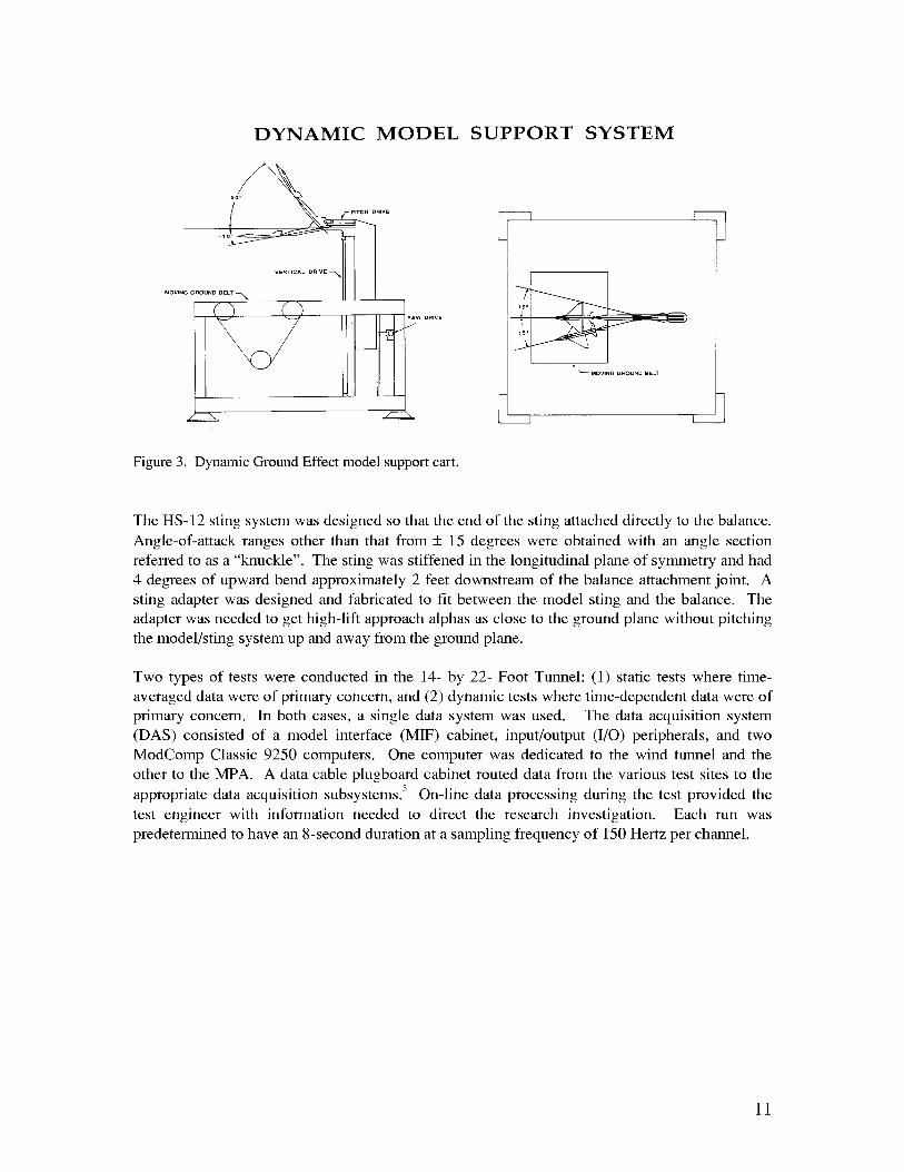
Figure 3. Dynamic Ground Effect model support cart.

The HS-12 sting system was designed so that the end of the sting attached directly to the balance.

Angle-of-attack ranges other than that from _+ 15 degrees were obtained with an angle section

referred to as a "knuckle". The sting was stiffened in the longitudinal plane of symmetry and had

4 degrees of upward bend approximately 2 feet downstream of the balance attachment joint. A

sting adapter was designed and fabricated to fit between the model sting and the balance. The

adapter was needed to get high-lift approach alphas as close to the ground plane without pitching

the model/sting system up and away from the ground plane.

Two types of tests were conducted in the 14- by 22- Foot Tunnel: (1) static tests where time-

averaged data were of primary concern, and (2) dynamic tests where time-dependent data were of

primary concern. In both cases, a single data system was used. The data acquisition system

(DAS) consisted of a model interface (MIF) cabinet, input/output (I/O) peripherals, and two

ModComp Classic 9250 computers. One computer was dedicated to the wind tunnel and the

other to the MPA. A data cable plugboard cabinet routed data from the various test sites to the

appropriate data acquisition subsystems. 5 On-line data processing during the test provided the

test engineer with information needed to direct the research investigation. Each run was

predetermined to have an 8-second duration at a sampling frequency of 150 Hertz per channel.

11

DGE DATA ACQUISITION

WIND TUNNEL

Balance

Accelerometel_

Tunnel

Pal'ametel_

CONTROL ROOM

Pitch

Height

Pitch H

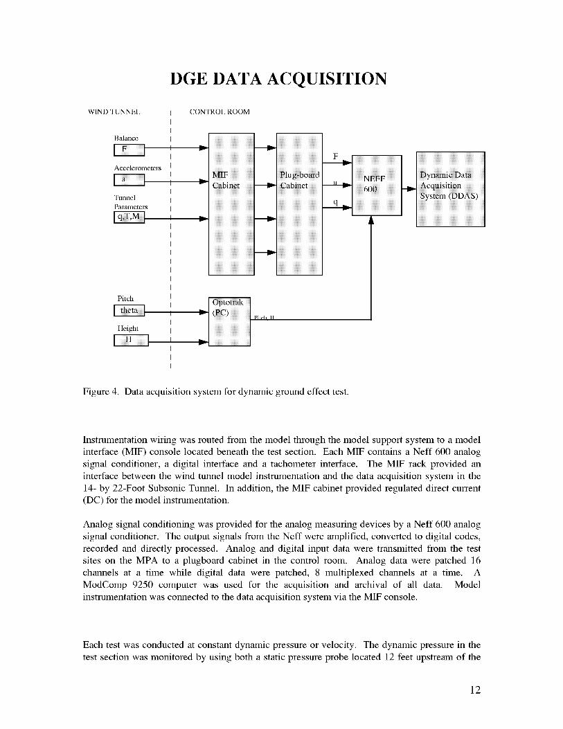
Figure 4. Data acquisition system for dynamic ground effect test.

Instrumentation wiring was routed from the model through the model support system to a model

interface (MIF) console located beneath the test section. Each MIF contains a Neff 600 analog

signal conditioner, a digital interface and a tachometer interface. The MIF rack provided an

interface between the wind tunnel model instrumentation and the data acquisition system in the

14- by 22-Foot Subsonic Tunnel. In addition, the MIF cabinet provided regulated direct current

(DC) for the model instrumentation.

Analog signal conditioning was provided for the analog measuring devices by a Neff 600 analog

signal conditioner. The output signals from the Neff were amplified, converted to digital codes,

recorded and directly processed. Analog and digital input data were transmitted from the test

sites on the MPA to a plugboard cabinet in the control room. Analog data were patched 16

channels at a time while digital data were patched, 8 multiplexed channels at a time. A

ModComp 9250 computer was used for the acquisition and archival of all data. Model

instrumentation was connected to the data acquisition system via the MIF console.

Each test was conducted at constant dynamic pressure or velocity. The dynamic pressure in the

test section was monitored by using both a static pressure probe located 12 feet upstream of the

12

testsectionandatotalpressureprobelocated59.4feetupstreamof thetestsectionin thesettlingchamber.Thestaticandtotalpressureprobeswereconnectedto a differential,fused-quartzbourdonpressuretransducerwithadigitalreadout.Thistransducerhasameasuredaccuracyof _+0.08psfof thefull-scalereading.Thedifferentialpressurereadingbetweenthestaticandtotalpressurereadingsis referredto astheindicateddynamicpressure,qind. Thisindicateddynamicpressureis relatedto the actualdynamicpressureof thetest sectionby meansof calibrationcurvesthat havebeendeterminedfor the differenttest-sectionconfigurations. No wallcorrectionswereimplementedin thecode. Thetestwasrunwith theboundarylayerremovalsystemin place. A testReynoldsnumberof approximately7 x 106andMach= 0.24wasmaintainedby adjustingthetunnelspeed.

Instrumentation

During the dynamic test, vibrations from the driving system were introduced into the measured

loads of the system. Accelerations on the model were measured and used to correct balance

forces. The vibrations were removed by measuring the accelerations of the system, calculating the

inertial loads from these accelerations, and then subtracting the inertial loads from the balanceforces.

Actual forces and moments were obtained by correcting all balance component test data for the

applicable component interaction data that were recorded during the balance calibration. Force

and moment measurements were made using the VST2 six component strain gauge balance. The

VST2 has a calibration range of _+1000 pounds in the normal direction,_+500 pounds in the axial

direction, _+4000 in-pounds of pitching moment, _+3000 in-pounds of rolling moment, _+3000 in-

pounds of yawing moment, and _+500 pounds in the side direction. Interactions between the

components were accounted for using a 6 x 27 matrix provided with the balance.

An Optotrak System measured pitch angle and height above the ground. Two cameras were set

up in the ceiling of the wind tunnel to view six infrared diodes on the model. These markers or

strobers provided height (above ground plane) and the model pitch angle measurements. A

Pentium based PC having a 2-channel I/O card provided the data acquisition for the system. The

PC based system provided a sampling rate of approximately 50 samples/sec for each channel.

Synchronization was provided between this system and the ModComp through a system of

interrupts initiated by the ModComp. The ModComp provided integration of the data packets

originating from the Optotrak, i.e, for two channels of data (pitch and height) into the database tobe archived.

Six Endevco model 7290A-10 accelerometers were used to measure model accelerations. These

accelerations have a range of_+10 g and a frequency response of 0 to 500 Hz. The accelerometers

were positioned in an orthogonal layout on the models, as shown in Figures 5 and 6.

13

Measurement Technique

The basis for this analysis and computation of the unsteady motion of a flight vehicle is to treat

the model of the vehicle as a single rigid body with six degrees of freedom. The mathematical

model is simplified further by treating Earth as flat and stationary in inertial space. The rigid

body equations are derived by applying Newton's laws to an element of the model and

calculating the summation of all the forces that act upon all the elements in the model. The

equation relates the resultant external aerodynamic force on the model to the motion of thereference center.

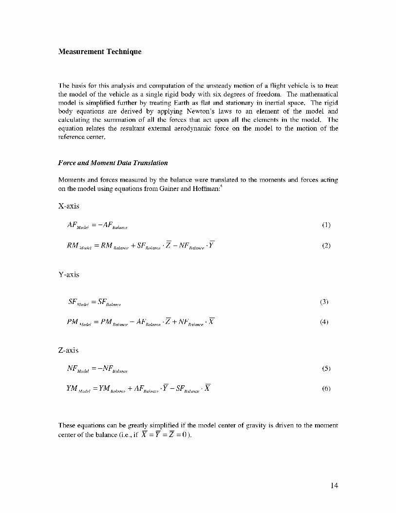
Force and Moment Data Translation

Moments and forces measured by the balance were translated to the moments and forces acting

on the model using equations from Gainer and Hoffman: 6

X-axis

AFModel = -AFBal .... (1)

Rm Modd = RM Bd .... + SFBd .... • Z -- NFBd .... "_- (2)

Y-axis

SFModel = SFBal .... (3)

PM Model= PMB_l .... - AFB_l.... •Z + NFB_ l.... •X (4)

Z-axis

NFModel = -NFB_l ....

YM Model = YM Bal.... "F AFBa l.... " Y - SFBal .... • X

(5)

(6)

These equations can be greatly simplified if the model center of gravity is driven to the moment

center of the balance (i.e., if X = Y = Z = 0 ).

14

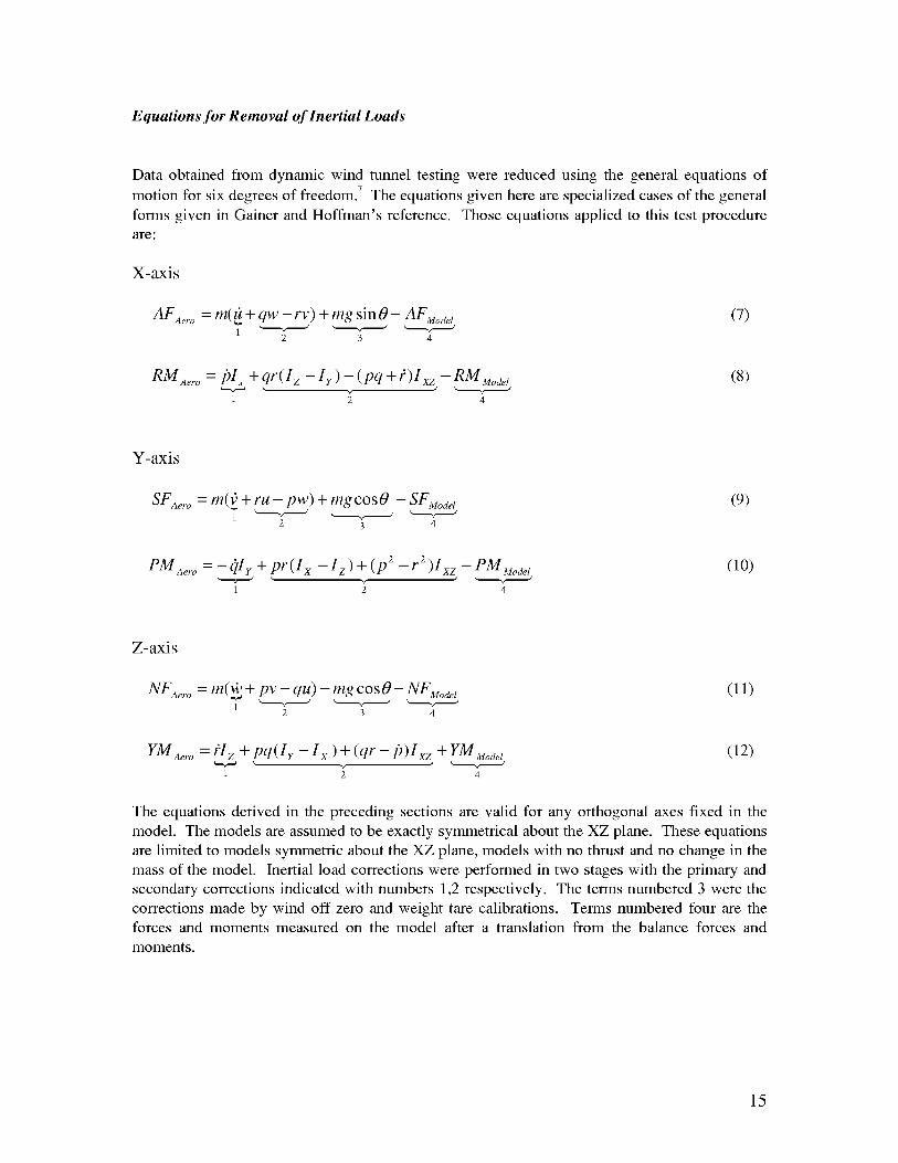
Equations for Removal of Inertial Loads

Data obtained from dynamic wind tunnel testing were reduced using the general equations of

motion for six degrees of freedom. 7 The equations given here are specialized cases of the general

forms given in Gainer and Hoffman's reference. Those equations applied to this test procedureare:

X-axis

AFAe,.o = m(_ + qw - rv) +mg sin 0 - AFModel (7)

2 3 4

RM Ae,.o = DI_ + qr( I z - I r ) - (pq + ?)Ixz- RM Mode, (8)

Y-axis

SFaero = m(_ + ru - pw) + mgcosO - SFModel (9)

2 3 4

PMAero = -(]Iy +pr(I x -Iz)+(p 2 r 2- )Ixz-_PMMode l (10)1 _ 4

Z-axis

NFAe,.o = m(_ + pv - qu) -mg cos0 - NFModel (11)1 _ _

2 3 4

YM Ae,.o = ?I z + pq(I r - I x ) + (qr - D)Ixz + YM Mode, (12)

The equations derived in the preceding sections are valid for any orthogonal axes fixed in the

model. The models are assumed to be exactly symmetrical about the XZ plane. These equations

are limited to models symmetric about the XZ plane, models with no thrust and no change in the

mass of the model. Inertial load corrections were performed in two stages with the primary and

secondary corrections indicated with numbers 1,2 respectively. The terms numbered 3 were the

corrections made by wind off zero and weight tare calibrations. Terms numbered four are theforces and moments measured on the model after a translation from the balance forces and

moments.

15

E_

o

_J

_o

_JE_

_o

o

_J

o

Linear Accelerations

Accelerometer measurements were combined to calculate linear and angular accelerations. The

accelerations were then integrated providing the velocity calculations. Detailed descriptions of

these calculations are presented in the following sections.

Axial acceleration, x-axis

it = A6 -awo Z - lg(sin 0) (13)

Side acceleration, y-axis

A5- A3

9 = A3 + lat_l'X"SF"+ latJl'X"St_''Ixdist31- awoz (14)

Normal acceleration, z-axis

A4- A2

= a2 + ixdist41+ ixdistzl Ixdist21- awo_ - lg(1 - cos 0) (15)

Angular Accelerations

Roll angular acceleration

A2 - A1

D = ydistl + ydist2

Pitch angular acceleration

(16)

A4- A2

gl = Ixdist21 + Ixdist41 (17)

18

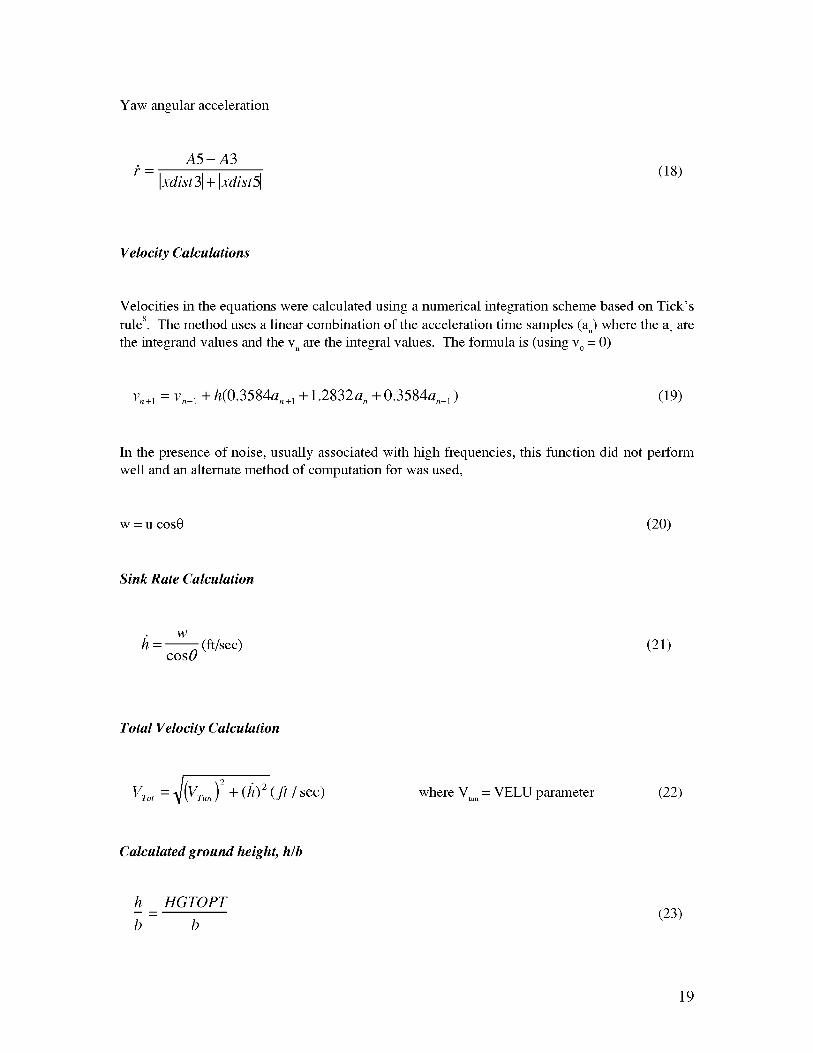
Yawangularacceleration

A5- A3

/ - Ixdist31+ Ixdist51 (18)

Velocity Calculations

Velocities in the equations were calculated using a numerical integration scheme based on Tick's

rule s. The method uses a linear combination of the acceleration time samples (a) where the an are

the integrand values and the v n are the integral values. The formula is (using v 0= 0)

v.+ 1 = v._l + h(0.3584a.+_ + 1.2832a. + 0.3584a.__ ) (19)

In the presence of noise, usually associated with high frequencies, this function did not perform

well and an alternate method of computation for was used,

w = u cos0 (20)

Sink Rate Calculation

/_ = w (ft/sec) (21)COS0

Total Velocity Calculation

where Vtu,,= VELU parameter (22)

Calculated ground height, hlb

h HGTOPTm

b b(23)

19

Flight Path Angle

(24)

Angle of Attack

or = 0 - 7' (25)

Corrected Dynamic Pressure

V o,qco,-r = q (lbs/ ft ) (26)

Note that the corrected dynamic pressure measurement was not used in these calculations to

conform with the static data reduction which was reduced using the QU parameter.

Corrected Force�Moment Coefficients

The normal-force coefficient, corrected for inertial loads is

NFAero

CN .... -- qco,-,-S (27)

The axial force coefficient, corrected for inertial loads is

AFAe,-oC -

A_°rr q_o,-,-S(28)

20

The pitching moment coefficient corrected to the model reference center and for inertialloads is

PMaer° (29)CM.... -- qco,TS-(

Performance Coefficients

The calculated lift coefficient, CLis defined to be

CL = CN.... COSO_--Ca_orr sino_ (30)

The calculated drag coefficient, CDis defined to be

C_ = Cu.... sin o_ + Ca_or,COSO_ (31)

21

Results and Discussion

One of the purposes of testing a model in the wind tunnel is to estimate the aerodynamic forces

the full scale vehicle will experience during operation. Distinct differences between data

obtained from steady-state wind-tunnel testing (constant height above ground) and dynamic flight

data (descending to the ground) were documented during a series of flight tests of low-aspect

ratio aircraft beginning in the late 1960s. 9 Subsequent wind-tunnel experiments in which the.... i0 ii 12

dynamic conditions of descending flight were simulated verified this dlstmcUon. ' ' The

distinction has also been confirmed through recent flight testing which has identified trends

dependent on sink rates. 13'14 The development of a ground-based technique at NASA for the

measurement of dynamic or time-dependent ground effects was driven by the existence of these

large discrepancies between flight test data and conventional wind tunnel ground effects tests for

supersonic transport aircraft with high swept wing configurations. The experiment was designed

to test the hypothesis that aspect ratio or sweep angle along with rate of descent might be an

important parameter in determining actual ground effects. Because ground effects tend to be

more significant for low-aspect ratio aircraft, the current development of high-speed civil

transport aircraft which use slender wing configurations has motivated research into this field.

In order to evaluate the dynamic ground effects of low aspect ratio and highly swept wing

configurations, the aerodynamic characteristics of an unswept elliptic wing model and two highly

swept wing models were tested in the subsonic wind tunnel. The elliptic wing model, which had

been used in this same wind tunnel on previous tests, enabled validation of the test method by

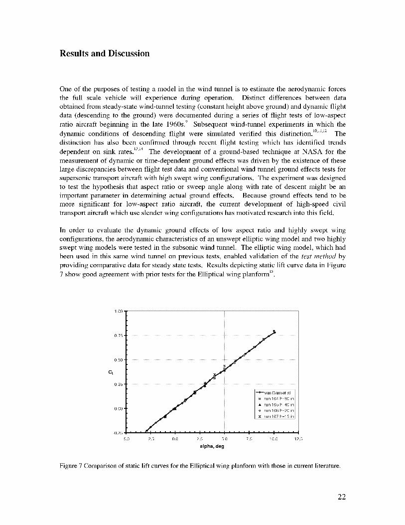
providing comparative data for steady state tests. Results depicting static lift curve data in Figure

7 show good agreement with prior tests for the Elliptical wing planform 15.

1.00 '

0.75 '

0.50 '

eL

0.25 '

0.00 '

0.25

5.0

metal I

f e:_ run 104 h=80 in I

J * run105 h=40 inl

J e, run 106 h=20 in I

........... i ...... I i-ruili7h 151hi

2.5 0.0 2.5 5.0 7.5 10.0 12.5

alpha, deg

Figure 7 Comparison of static lift curves for the Elliptical wing planform with those in current literature.

22

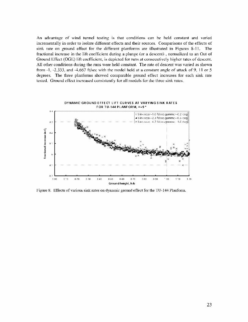
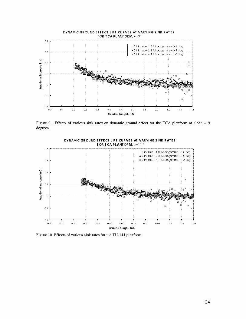
An advantage of wind tunnel testing is that conditions can be held constant and varied

incrementally in order to isolate different effects and their sources. Comparisons of the effects of

sink rate on ground effect for the different planforms are illustrated in Figures 8-11. The

fractional increase in the lift coefficient during a plunge (or a descent), normalized to an Out of

Ground Effect (OGE) lift coefficient, is depicted for runs at consecutively higher rates of descent.

All other conditions during the runs were held constant. The rate of descent was varied as shown

from -1, -2.333, and -4.667 ft/sec with the model held at a constant angle of attack of 9, 11 or 5

degrees. The three planforms showed comparable ground effect increases for each sink rate

tested. Ground effect increased consistently for all models for the three sink rates.

O4

O3

,-= 02

N

"_ o

Ol

DYNAMIC GROUND EFFECT LIFT CURVES AT VARYING SINK RATES

FOR TU-144 PLANFORM,(z=9 °

_:_S ink rate=-1.0 [t/sec, gamma=-0.2 deg

A S ink rate=-2.3 [t/sec, gamma=-0.5 deg× S ink rate=-4.7 ft/sec aroma=-1.0

x

i×

02

000 010 020 030 040 050 060 070 080 090 I O0 110

Ground height, h/b

Figure 8. Effects of various sink rates on dynamic ground effect for the TU-144 Planform.

1 20

23

O4

O3

,_c o2

m,==_. 0 1

i_ 0

01

O2

O0

Figure 9.

degrees.

DYNAMIC GROUND EFFECT LIFT CURVES AT VARYING SINK RATESFOR TCAPLANFORM, o_=9°

1A S ink rate=-2.3 ft/sec, gamma=-0.5 deg / 1

x S ink rate=-4.7 R/sec, gamma=-1.0 deg / /

×_

01 02 03 04 05 06 07 08 09 10 11 12

Ground height, h/b

Effects of various sink rates on dynamic ground effect for the TCA planform at alpha = 9

O4

O3

d,I2 02

,_ 01

,._oo

01

DYNAMIC GROUND EFFECT LIFT CURVES AT VARYING SINK RATES

FOR TCA PLANFORM, _=11 °

1

::::Sink rate=-1.0 R_ ec,gamma=-0.2 deg /A Sink rate=-2.3 R_ec,gamma=-0.5 deg

/

x Sink rate=-4.7 R_ ec,,qamma=-1.0 deq

! x:

-- ::': _ _ X X

O2

000 010 020 030 040 050 060 070

Ground height, h/b

Figure 10 Effects of various sink rates for the TU-144 planform.

080 090 1 O0 1 10 1 20

24

0.4

0.3

0.2e-

t_

,-. 0.1

cO

m 0I,I.

-0.1

DYNAMIC GROUND EFFECT LIFT CURVES AT VARYING SINK RATES FOR

E L L IPT ICAL WING, c_,=5°

× Sink rate=-4.7 ft/sec,gamma=-1.0 deg

A Sink rate=-2.3 ft/sec,gamma=-0.5 deg

N

X

i i ix_i _ i i i x i

-0.2 t i t t i

0.00 0.10 0.20 0.30 0.40 0.50 0.60 0.70 0.80

Ground height, h/b

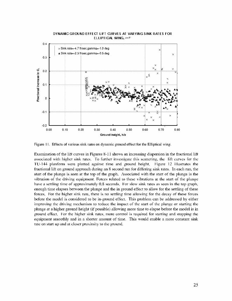
Figure 11. Effects of various sink rates on dynamic ground effect for the Elliptical wing.

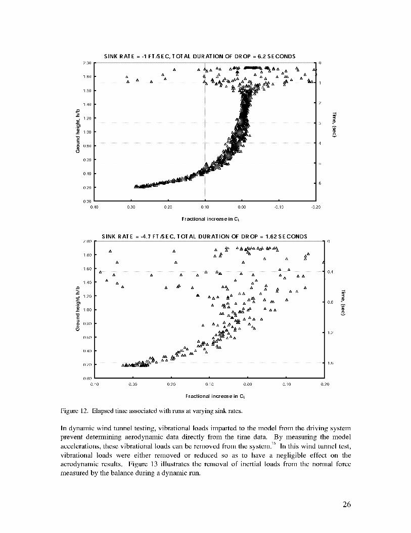
Examination of the lift curves in Figures 8-11 shows an increasing dispersion in the fractional lift

associated with higher sink rates. To further investigate this scattering, the lift curves for the

TU-144 planform were plotted against time and ground height. Figure 12 illustrates the

fractional lift on ground approach during an 8 second run for differing sink rates. In each run, the

start of the plunge is seen at the top of the graph. Associated with the start of the plunge is the

vibration of the driving equipment. Forces related to these vibrations at the start of the plunge

have a settling time of approximately 0.8 seconds. For slow sink rates as seen in the top graph,

enough time elapses between the plunge and the in ground effect to allow for the settling of these

forces. For the higher sink rate, there is no settling time allowing for the decay of these forces

before the model is considered to be in-ground effect. This problem can be addressed by either

improving the driving mechanism to reduce the impact of the start of the plunge or starting the

plunge at a higher ground height (if possible) allowing more time to elapse before the model is in

ground effect. For the higher sink rates, more control is required for starting and stopping the

equipment smoothly and in a shorter amount of time. This would enable a more constant sink

rate on start up and at closer proximity to the ground.

25

2.00

1.80

1.60

1.40

,,c1.20

1.00

0.80

o

0.60

0.40

0.20

0.00

0.40

SINK RATE = -1 FT/SEC, TOTAL DURATION OF DROP = 6.2 SECONDS

0.30 0.20 0.10 0.00 0.10

Fractional increase in eL

0

A

1

2

3

4

5

6

0.20

3m

tP

2.00

1.80

1.60

1.40

,,c1.20

.__,_@ 1.00

.O 0.80

o

0.60

0.40

0.20

0.00

0.40

SINK RATE = -4.7ET/SEC, TOTAL DURATION OF DROP = 1.62 SECONDS

i I I I I

0.30 0.20 0.10 0.00 0.10

0.4

30.8 -_

0.20

1.2

1.6

Fractional increase in eL

Figure 12. Elapsed time associated with runs at varying sink rates.

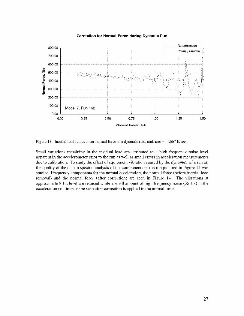
In dynamic wind tunnel testing, vibrational loads imparted to the model from the driving system

prevent determining aerodynamic data directly from the time data. By measuring the model

accelerations, these vibrational loads can be removed from the system, t6 In this wind tunnel test,

vibrational loads were either removed or reduced so as to have a negligible efl'ect on the

aerodynamic results. Figure 13 illustrates the removal of inertial loads from the normal force

measured by the balance during a dynamic run.

26

oOIJ.m

.EOZ

Correction for Normal Force during Dynamic Run

800.00

700.00

600.00

500.00

400.00

300.00

200.00

100.00

0.00

0.00

Model 7, Run 162

I I I I I I

0.25 0.50 0.75 1.00 1.25 1.50

Ground height, h/b

Figure 13. Inertial load removal for normal force in a dynamic rate, sink rate = -4.667 ft/sec.

Small variations remaining in the residual load are attributed to a high frequency noise level

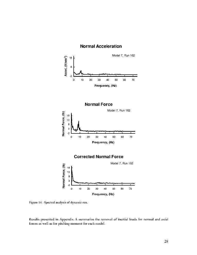
apparent in the accelerometer prior to the run as well as small errors in acceleration measurements

due to calibration. To study the effect of equipment vibration caused by the dynamics of a run on

the quality of the data, a spectral analysis of the components of the run pictured in Figure 14 was

studied. Frequency components for the normal acceleration, the normal force (before inertial load

removal) and the normal force (after correction) are seen in Figure 14. The vibrations at

approximate 9 Hz level are reduced while a small amount of high frequency noise (35 Hz) in the

acceleration continues to be seen after correction is applied to the normal force.

27

Normal Acceleration

-2

0 10

Model 7, Run 162

I I I I

20 30 40 50

Frequency, (Hz)

I I

60 70

Normal Force

Model 7, Run 162

18

13

8

I,..0 -2

z0 10 20 30 40 50 60 70

Frequency, (Hz)

Corrected Normal Force

18e"o 13o

u. 8

3E0 -2

Z

Model 7, Run 162

0 10 20 30 40 50 60 70

Frequency, (Hz)

Figure 14. Spectral analysis of dynamic run.

Results presented in Appendix A summarize the removal of inertial loads for normal and axial

forces as well as for pitching moment for each model.

28

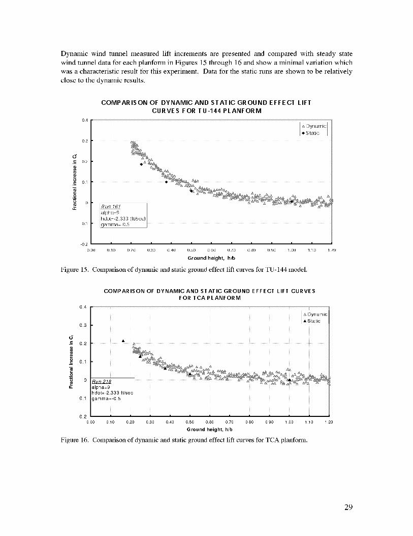
Dynamic wind tunnel measured lift increments are presented and compared with steady state

wind tunnel data for each planform in Figures 15 through 16 and show a minimal variation which

was a characteristic result for this experiment. Data for the static runs are shown to be relatively

close to the dynamic results.

0.4

0.3

tYi_ 0.2

e._ 0.1

u 0

COMPARISON OF DYNAMIC AND STATIC GROUND EFFECT LIFT

CURVES FOR TU-144PLANFORM

0.1

Dynamic

Static

_.

: _ : : :

alpha=9hdot=-2.333 ( rds ec)

Ig amma=-O.5 I

012 i i i i i i i i i i i

OIO0 0110 0120 0130 0140 0150 0160 0170 0180 0190 1100 1.10

Ground height, h/b

Figure 15. Comparison of dynamic and static ground effect lift curves for TU-144 model.

1.20

0.4

0.3

dI_ 0 .2

=_ ol.ii

.£0

u.

-0.1

COMPARISON OF DYNAMICAND STATIC GROUND EFFECT LIFT CURVESFOR TCAPLANFORM

_ Dynamic

_uo2_o | ....... _'_ _m_ _ _ 2,\_'_°_alpha=9 ]

hdot=-2.333 ft/sec

aroma=-0.5 J

-0.2 I I I I I I I I I I

OIO0 0II 0 0120 0130 0140 0150 0160 0170 0180 0190 I IO0 I II 0

Ground height, h/b

Figure 16. Comparison of dynamic and static ground effect lift curves for TCA planform.

1.20

29

0.4

COMPARISON OF DYNAMIC AND STATIC GROUND EFFECT LIFT CURVES FOR

FOR ELLIPTICAL WING PLANFORM

Dynamic ._

I • Static I

0.3 .....

.E 0.2 ........ _= i

o

._=o.1 =_ X_ _2c

0 _ i &

o 0LK

alpha = 5 ] _- :

-0.1 hdot=-2.333gamma=.0.5ft/sec .... _ x_i_ _

-0.2

0.00 0.10 0.20 0.30 0.40 0.50 0.60 0.70 0.80 0.90 1.00

Ground height, h/b

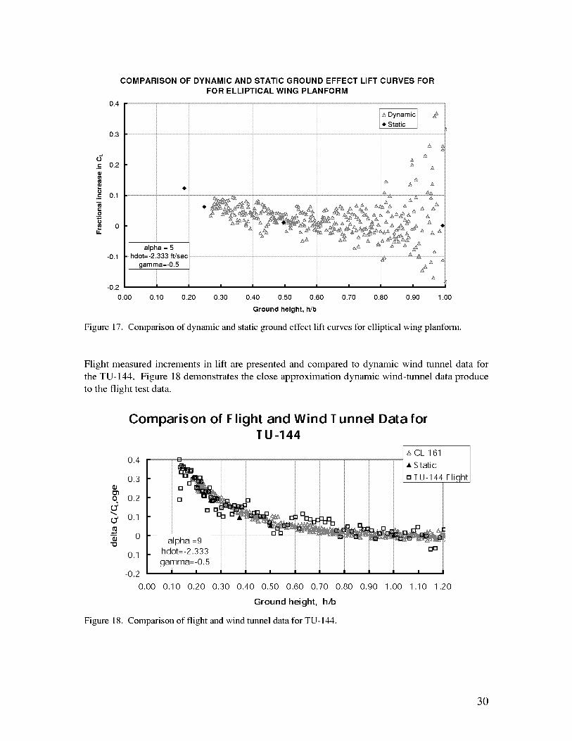
Figure 17. Comparison of dynamic and static ground effect lift curves for elliptical wing planform.

Flight measured increments in lift are presented and compared to dynamic wind tunnel data for

the TU-144. Figure 18 demonstrates the close approximation dynamic wind-tunnel data produce

to the flight test data.

qc_

"o

0.4

0.3

0.2

0.1

0

-0.1

-0.2

0.00

Comparison of F light and Wind I unnel Data forT g -144

F

..................° i _cL

• El --_: i

i i _ oi i i i

• hdot=-2.333 ........ no

Flight

gamma=-O.5i i ,

0.10 0.20 0.30

I I I I I I I I

0.40 0.50 0.60 0.70 0.80 0.90 1.00 1.10 1.20

Ground height, h/b

Figure 18. Comparison of flight and wind tunnel data for TU-144.

30

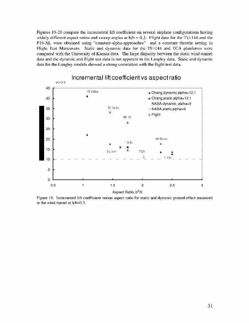
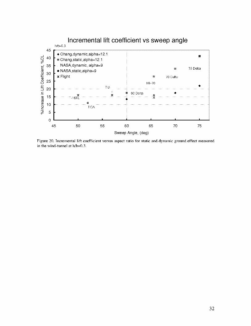
Figures 19-20 compare the incremental lift coefficient on several airplane configurations having

widely different aspect ratios and sweep angles at h/b = 0.3. Flight data for the TU-144 and the

F16-XL were obtained using "constant-alpha-approaches" and a constant throttle setting in

Flight Test Maneuvers. Static and dynamic data for the TU-144 and TCA planforms were

compared with the University of Kansas data. The large disparity between the static wind-tunnel

data and the dynamic and flight test data is not apparent in the Langley data. Static and dynamic

data for the Langley models showed a strong correlation with the flight test data.

45

40

h/b=0.3Incremental lift coefficient vs aspect ratio

75Delta 4, Chang ,dynamic,alpha=l 2.1

_=_Chang,static,alpha=l 2.1

:: NASA,dynamic, alpha=9

70 Delta ::<NASA,static,aloha=9.

XB-70 x Flight

O

60 Delta

4, :::F 16-XL _=_

X

TU-144 :X TCA _.

F-104

I I I I

0.5 1 1.5 2 2.5 3

Aspect Ratio, b2/S

Figure 19. Incremental lift coefficient versus aspect ratio for static and dynamic ground effect measuredin the wind-tunnel at h/b=0.3.

31

Incremental lift coefficient vs sweep angleh/b=0.3

45

d

0 40o_

35c-(D

._o 30

8 25

_ 20¢--

• 15fflt_

_ lO0¢--

_ 5

0

45

4, Chang,dynamic,alpha=12.1

_--.-_Chang,static,alph a= 12.1

NASA,dynamic, alpha=9

NASA,static,alpha=9

x Flight

x_

_--.--_ 75 Delta

[-':_ 70 Delta

XB-70

TU-

: _ 60 Delta

F:16XL @ X

TCA

I I I I I I

50 55 60 65 70 75

Sweep Angle, (deg)

Figure 20. Incremental lift coefficient versus aspect ratio for static and dynamic ground effect measured

in the wind-tunnel at hfo=0.3.

32

APPENDIX A Inertial Loads Removal

Balance force and moment data for each model in the test facility contained significant inertial

loads due to carriage motion and support dynamics. Six accelerometers were placed in an

orthogonal layout in order to measure the inertial loads on the model. Prior to a set of runs for

each model, a wind-off weight tare and three calibration runs (pitch, yaw, roll) were completed.

The weight tare calculated the weight of the model and provided the system with additional

correction factors for the weight factor of each model. Extensive data is available from three

normal, two axial, and two side accelerometers. This section addresses the method of correction

to the balance loads developed on the latest data.

The calibration run consisted of a wind-off, static run during which the model was bumped or

"jogged" in one of three directions (pitch, yaw, roll) to induce inertial loads. The model was kept

at a constant height of 50" above the ground and at a constant angle of attack. The data set for

these runs was curve fitted in linear and multiple regressions for the optimal removal of inertialloads.

Additional calibration was performed for each acceleration in order to remove a bias or zero

offset. This was performed by averaging each acceleration over a 0.5 second (75 sample) period

at the beginning of each run (prior to any movement of the mast) and using this value as a zero

offset which was subtracted out of all remaining samples per acceleration.

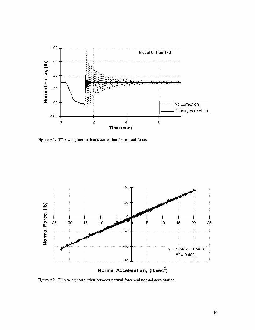
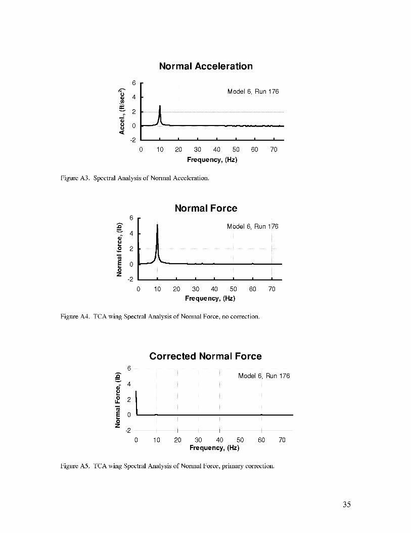
Results of the correction for inertial loads are presented for each force and moment. Subtraction

of the inertial loads accounted for the removal of most of the measurable vibrational effects.

Secondary accelerations from coupled velocity terms (2) in equations 7.0-12.0 had a negligible

effect on the removal of inertial loads. For tests without significant model velocities, the

correlation between the measured loads and associated accelerations provided a measure of errors

in the system. Models 6 and 7 show excellent correlation between either normal or axial loads

and corresponding accelerations. A spectral analysis exhibits frequencies associated with the

inertial loads. In addition, the spectral analysis pinpoints low level noise (at 1 Hz) and higher

frequencies (at 60 Hz) which interfered in some cases with the correction. Small variations

remaining in the residual load were attributed to the noise level of the signal as well as errors inacceleration measurements.

• External loads imparted on the system from striking it

• Impulses in the analog signal not resulting from actual loads

• Noise level of the signal

• Errors in acceleration measurements

33

IO0

,'-'- 60,,Qm

e-o 20

@I,,I.

m -20El_

oZ -60

-100

' Model 6, Run 176

:::,!!!,....',',',',;',:",t',',",',:",_4,',_,_J:,_,.,,,_..

,,,,,i,h,,.,:,,::,,,,,,. _.,,__7.., ,_,,,., ....,,,,,%,,,,,, , .,I i,'*/I i !!',',,,,i,',',r .',

,,_:,

:' [ ....... No correctionm

/

L Primary correctionI I I

0 2 4 6

Time (sec)

Figure A1. TCA wing inertial loads correction for normal force.

e',m

o"oL_

oI.K

EL_

oZ

.... 60 -

5 10 15 20 25

y = 1.848x - 0.7466R2= 0.9991

Normal Acceleration, (ft/sec 2)

Figure A2. TCA wing correlation between normal force and normal acceleration.

34

Normal Acceleration

u

uu,<

6

4

2

0

-2

0

Model 6, Run 176

10 20 30 40 50 60 70

Frequency, (Hz)

Figure A3. Spectral Analysis of Normal Acceleration.

6

e-,

v 4

.oo 2

m

t_

E 0o

Z-2

Normal Force

I I I I I I I

0 10 20 30 40 50 60 70

Frequency, (Hz)

Figure A4. TCA wing Spectral Analysis of Normal Force, no correction.

6e-,

m

.oo 2ii

m

t_

E 0o

Z-2


Model 6, Run 176

I

10

A

I I I I I I

20 30 40 50 60 70Frequency, (Hz)

Figure A5. TCA wing Spectral Analysis of Normal Force, primary correction.

35

20

..Q 10i

,,o o

'_ -10

-20

Model 6, Run 176

:;,,• .',( ].

,I,,,',,',,ii( _, •, _,.

Primary correction

i0 2 4 6

Time (sec)

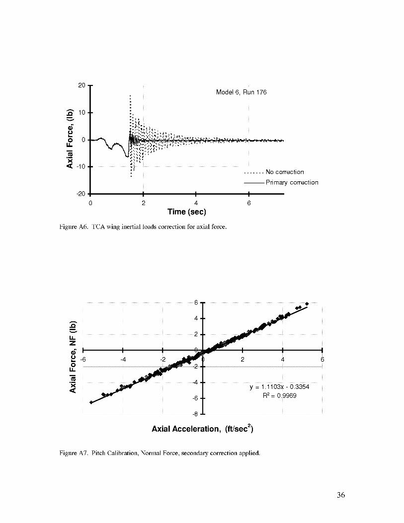
Figure A6. TCA wing inertial loads correction for axial force.

.

4

• 2

ii ii ii

i l l

2 4 6

y = 1.1103x - 0.3354

R2= 0.9969

Axial Acceleration, (ft/sec 2)

Figure A7. Pitch Calibration, Normal Force, secondary correction applied.

36

Axial Acceleration

u0.8

0.4,,.,

'_ 0uu,< -0.4

0 10 20 30 40 50 60 70

Frequency, (Hz)

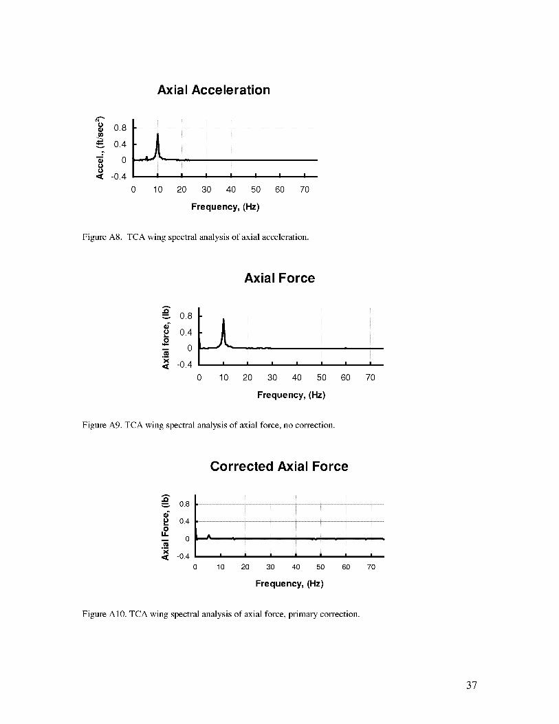
Figure A8. TCA wing spectral analysis of axial acceleration.

Axial Force

..Q_. 0.8

P 0.40

-- 0.__x,< -0.4

0 10 20 30 40 50 60 70

Frequency, (Hz)

Figure A9. TCA wing spectral analysis of axial force, no correction.

Corrected Axial Force

..Q0.8

0.40

LI.0

X,,_ -0.4

0

I I I I I I I

10 20 30 40 50 60 70

Frequency, (Hz)

Figure A10. TCA wing spectral analysis of axial force, primary correction.

37

120

-- 60

'_ 0c

E0 -60

c -120,m

o-180

IX

-24O

Model 6, Run 176

....... Nocorrection

-- Primary correction! ! =

0 2 4 6

Time (sec)

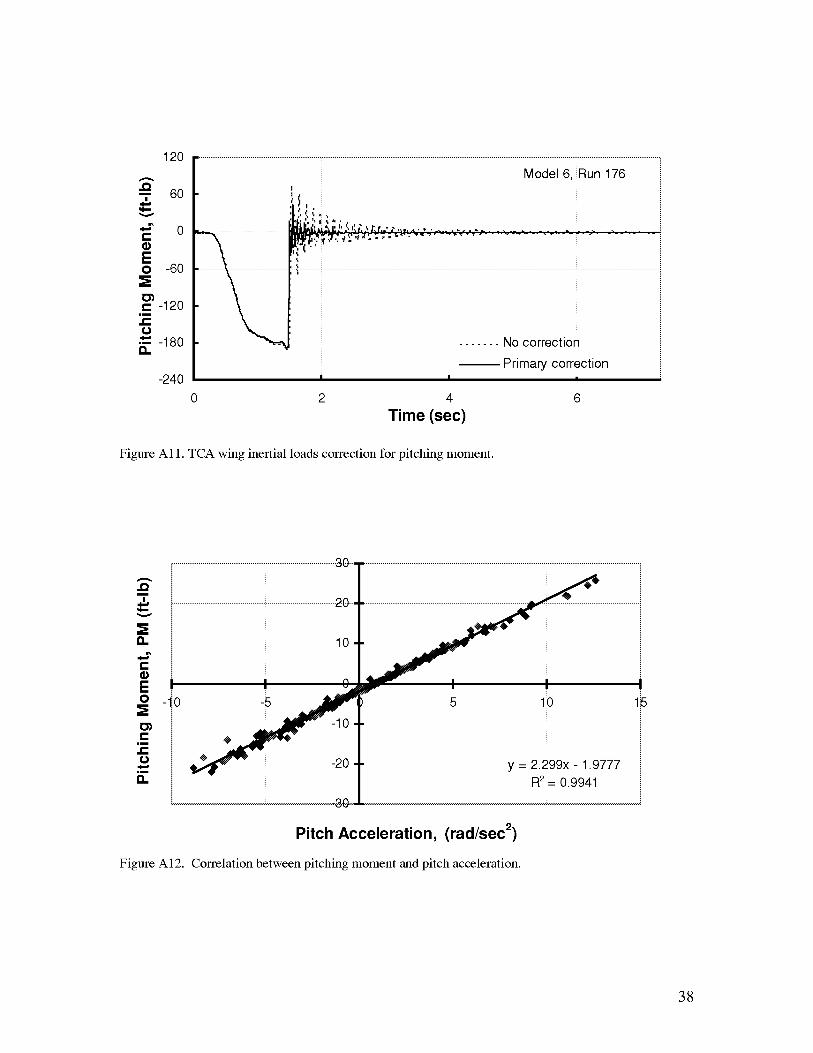
Figure A11. TCA wing inertial loads correction for pitching moment.

e',,4,'

IX

e-

Eo

e-c-o

IX

2_

-0

y = 2.299x - 1.9777R2= 0.9941

Pitch Acceleration, (rad/sec 2)

Figure A12. Correlation between pitching moment and pitch acceleration.

38

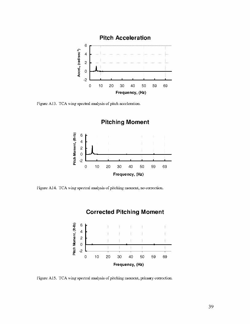
Figure A13.

¢,1

¢J

¢J¢J

6

4

2

0

-2

0

Pitch Acceleration

I I I I I I I

10 20 30 40 50 59 69

Frequency, (Hz)

TCA wing spectral analysis of pitch acceleration.

" 6

4e-

2EO

0e-

,_o -213.

Pitching Moment

0 10 20 30 40 50 59 69

Frequency, (Hz)

Figure A14. TCA wing spectral analysis of pitching moment, no correction.

Corrected Pitching Moment

i ' '_2 i i i i i i i13.

0 10 20 30 40 50 59 69

Frequency, (Hz)

Figure A15. TCA wing spectral analysis of pitching moment, primary correction.

39

120

d 40

IJ.

Z -40

-80

Model 7,Run 149

],Q

.:::::: _::- ::-.'.,',: .;:,, _,; ', _ '.; _,

L, ,, ,, , I ) , 0. _,'' "l ''|H'lll ''' I,:'m I _tm,r " ,_ /l_ ,

X, ilPIl'l",,""',,,*","'. ,,'_'\,""",,_,'_2_''_ _7''''_ _",m ,,, , . l, ,. ,,,, ._

_. 11.".'.',.'° ..' .... . '..' ,,. J, -" . ",,, ,, ,m,,h b_

,,,, ,,,I ,I ,m,. m .i i", ,F,,,,.......,%, ,,,%_=,

_"-_: ;, _.,, ....... No correchon

! ' --Primary correction

0 2 4 6

Time (sec)

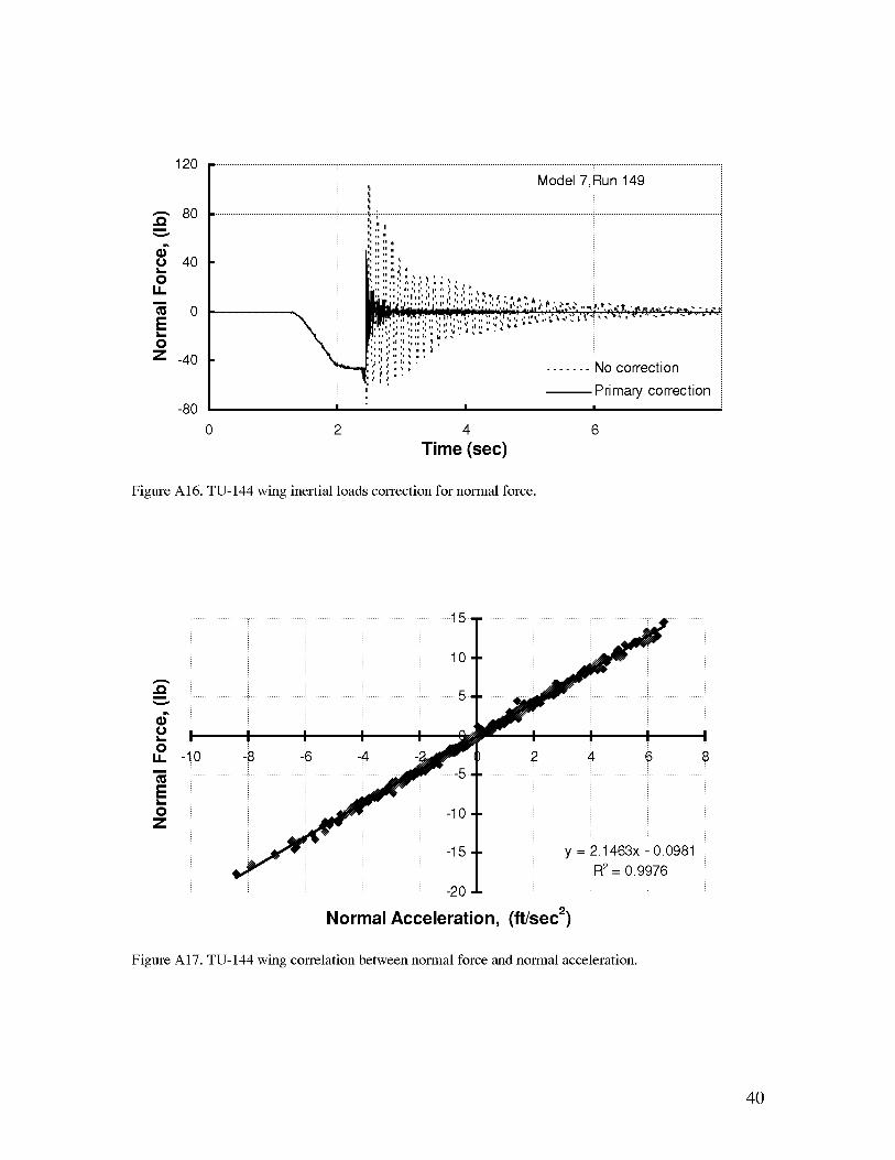
Figure A16. TU-144 wing inertial loads correction for normal force.

10

e'li

o"O

oI,Ki

EoZ

• 5

t5 y = 2.1463x - 0.0981R 2 = 0.9976

-20

Normal Acceleration, (ft/sec _)

Figure A17. TU-144 wing correlation between normal force and normal acceleration.

4O

NORMAL ACCELERATION

u

v

uu

10

6

2

-2

0 10 20 30 40 50 60 70

Frequency, (Hz)

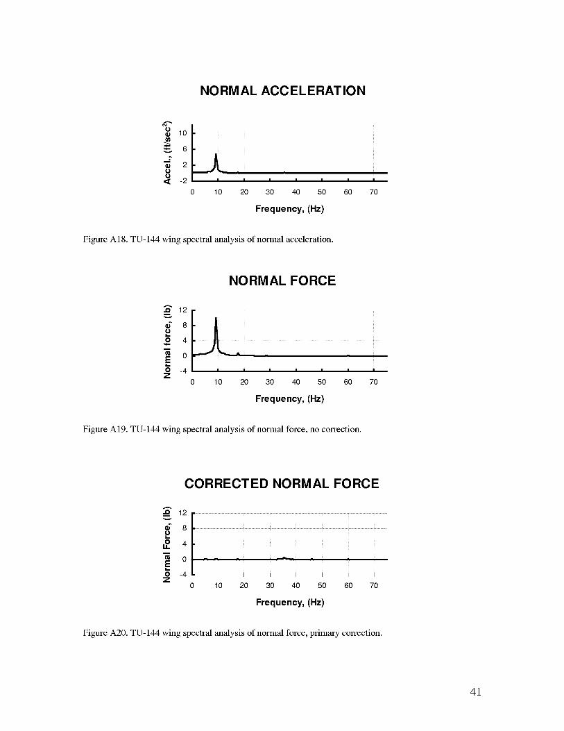
Figure A18. TU-144 wing spectral analysis of normal acceleration.

NORMAL FORCE

mv

.uO

m

.EO

Z

12

8

4

0

-4

0 10 20 30 40 50 60 70

Frequency, (Hz)

Figure A19. TU-144 wing spectral analysis of normal force, no correction.

CORRECTED NORMAL FORCE

•_ 12mv

G 8.uO 414.

m

o= 0

.EO -4

Z• I I I I I

0 10 20 30 40 50

Frequency, (Hz)

m

I I

60 70

Figure A20. TU-144 wing spectral analysis of normal force, primary correction.

41

30

e'li

t_L_

oiii

.i

x

20

10

-10

-20

0

,,,, Model 7, Run 149I

I: ....... No correction

-- Primary correction

2 4 6

Time (sec)

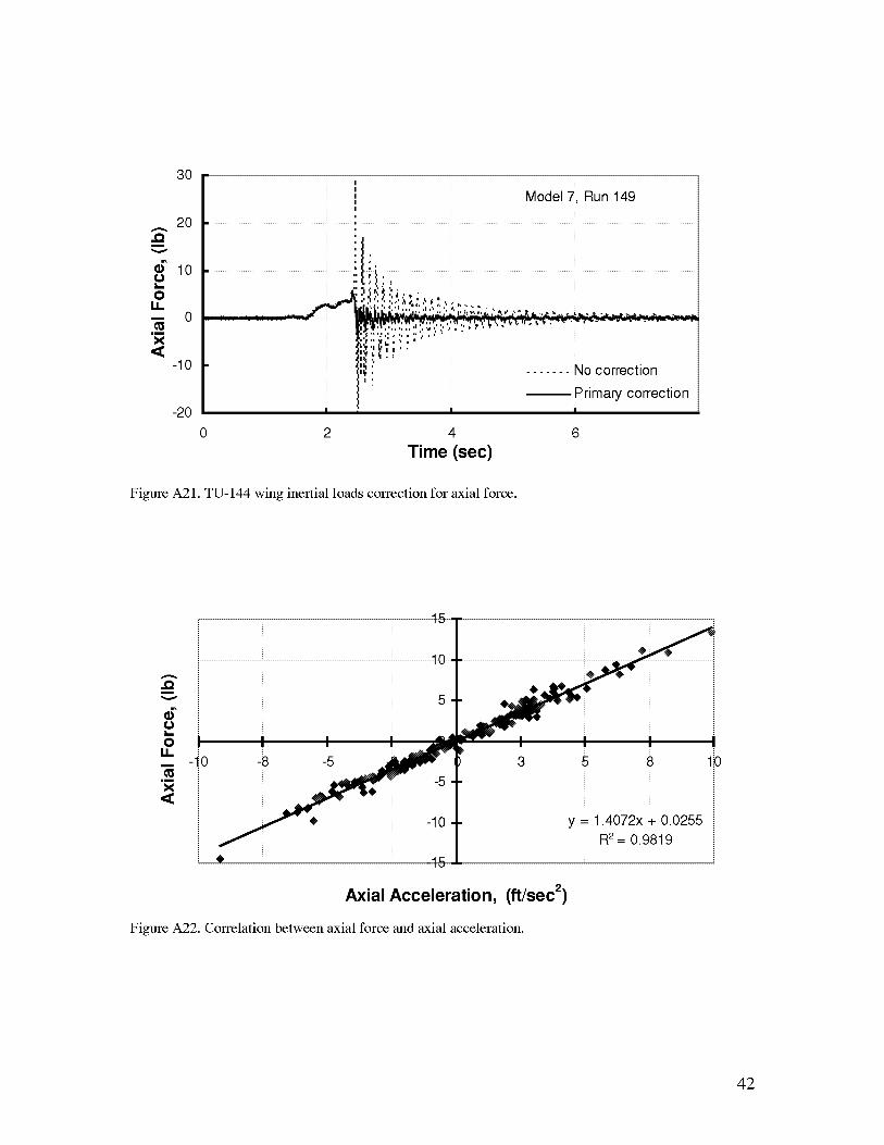
Figure A21. TU-144 wing inertial loads correction for axial force.

e'li

t_x_

oiii

x

| |

5 8

y = 1.4072x + 0.0255

R2= 0.9819


Figure A22. Correlation between axial force and axial acceleration.

42

AXIAL ACCELERATION

_, 2tj

1.5

'*-' 1

:" 0.5

o 0u

"_ -0.5

0 10 20 30 40 50 60

Frequency, (Hz)

70

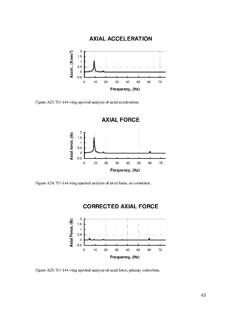
Figure A23. TU-144 wing spectral analysis of axial acceleration.

AXIAL FORCE

2.Q_" 1.5

=,9. 10 0.5

.m 0x

,,_ -0.5

0 10

m

20 30 40 50

Frequency, (Hz)

^

6O 7O

Figure A24. TU-144 wing spectral analysis of axial force, no correction.

CORRECTED AXIAL FORCE

2.Qm

1.5

.u 1o 0.5u.

o.,_,,_ -0.5 I I I I I I I

0 10 20 30 40 50 60 70

Frequency, (Hz)

Figure A25. TU-144 wing spectral analysis of axial force, primary correction.

43

180

,,Qm

|

C

EO

C.m

..CO

IX

120

6O

0

-60

-120

-180

-240

Model 7, Run 149

[

° _J° :

-- Primary correction! ! !

2 4 6

Time (sec)

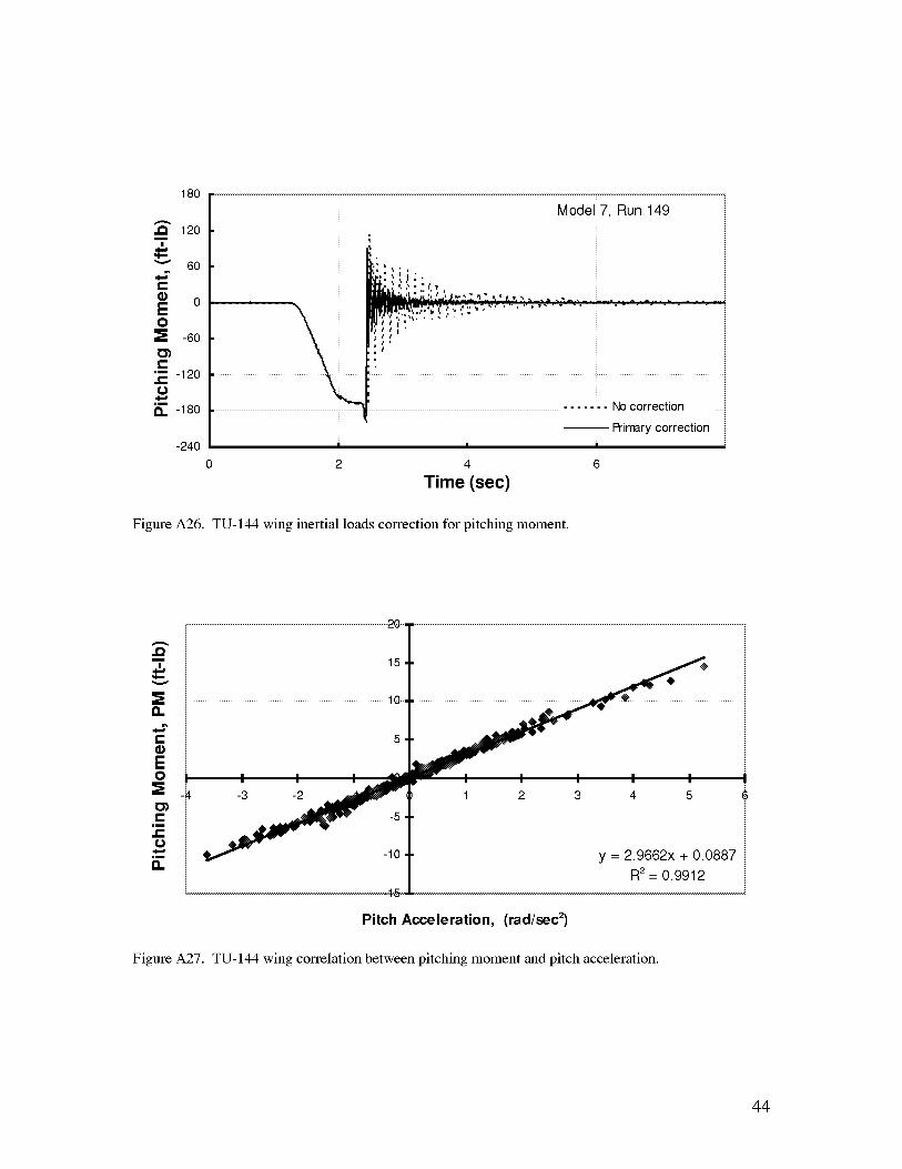
Figure A26. TU-144 wing inertial loads correction for pitching moment.

e',m

Eo

IX

Figure A27.

15 • A_* __f_

10- _'

5-

I I I I _¢_,

-5 •

_i::R 2 = 0.9912

,t-5_


TU-144 wing correlation between pitching moment and pitch acceleration.

44

tj

"o

v

tjtj

4

3

2

1

0

-1

0

Pitch Acceleration

10 20 30 40 50

Frequency, (Hz)

59 69

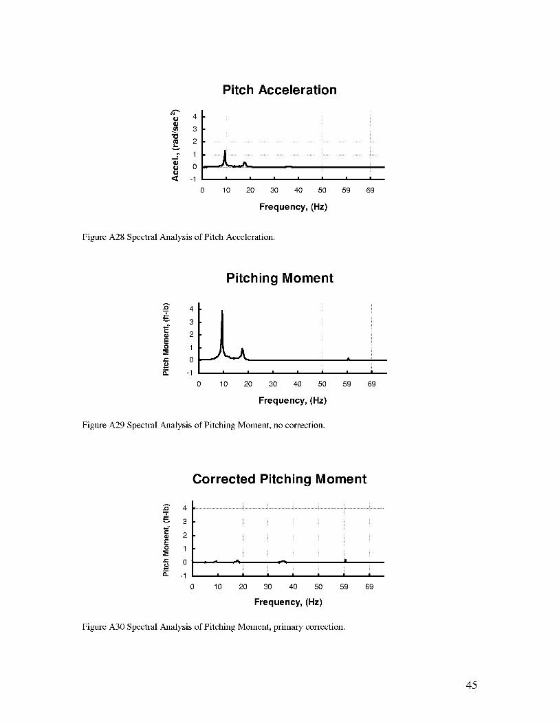
Figure A28 Spectral Analysis of Pitch Acceleration.

Pitching Moment

..Qm

&t-"

EO

e-"

,._o13.

4

3

2

1

0

-1

0 10 20 30 40 50 59 69

Frequency, (Hz)

Figure A29 Spectral Analysis of Pitching Moment, no correction.


_' 4

3t-" 2Eo 1

-= 0

o. -1

0

I I I I I I I

10 20 30 40 50 59 69

Frequency, (Hz)

Figure A30 Spectral Analysis of Pitching Moment, primary correction.

45

20

10i

oI--

oI,.I. 0i

c_EI--

o -10Z

-20

40

Model 10, Run 20

%i ,, ,i . _' o _% ,_,P i ', _ f h,

_, ,I '. ,. .I ,\ ,, ,, ,'. _i ,. ,I i, ., ,I , :. _' ', ;, .. ,' *, . •

..... , ,, _ ,, , ,:, . ,', : ,,1 ,'. ', ,.,, ,: .';. ,, _, ,: ,, ,, ,, , ,

, . ,, ,, . ,, i: ',: :

._ ...... ............; , ,. ,, ,: ,, ,, ,o .. . ,

'.' _ ,. ,,I;

l ....... Nocorrection/ -- Primary correction/ I i I

50 60 70

Time (sec)

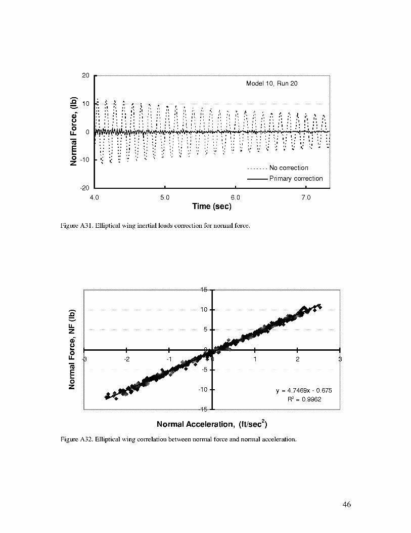
Figure A31. Elliptical wing inertial loads correction for normal force.

A

i

iiZ

o"o!._

oiii

E!._

oZ

5.

I I I

y = 4:7469x - 0:675R2= 0.9962

Normal Acceleration, (ft/sec 2)

Figure A32. Elliptical wing correlation between normal force and normal acceleration.

46

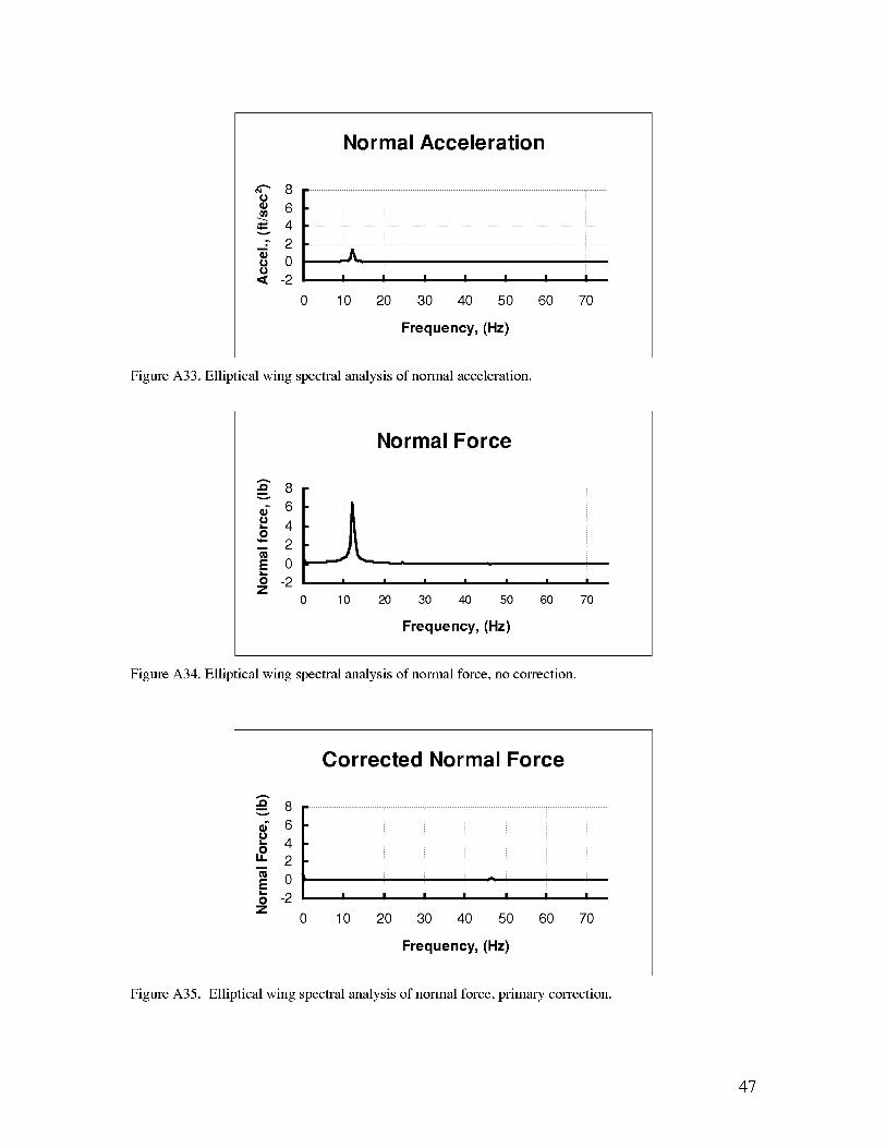
Normal Acceleration

_" 8u

== 6_. 4v

28 0u'==: -2 I I I I i I I

10 20 30 40 50 60 70

Frequency, (Hz)

Figure A33. Elliptical wing spectral analysis of normal acceleration.

Normal Force

__" 8v

6.u 4O

i 20

-2

0 10 20 30 40 50 60 70

Frequency, (Hz)

Figure A34. Elliptical wing spectral analysis of normal force, no correction.


8

G 6.u 4Ou. 2m

-2Z

A

I I I I I I I

0 10 20 30 40 50 60 70

Frequency, (Hz)

Figure A35. Elliptical wing spectral analysis of normal force, primary correction.

47

15.0

,,Qm

e"o

oLI.

X,<

100

5.0

0.0

-5.0

Model 10, Run 20

,a i

• .,;I.. ,,',U" nil " I

", ,.'J :1 ,; _ . .I

H I

r • a _a , ,. _," ' v _ " _ t _ _ _, • _ i. ,

i I

-10.0 ....... No correction

-- Primary correction-15.0 i i i , ,

2.0 3.0 4.0 5.0 6.0 7.0

Time (see)

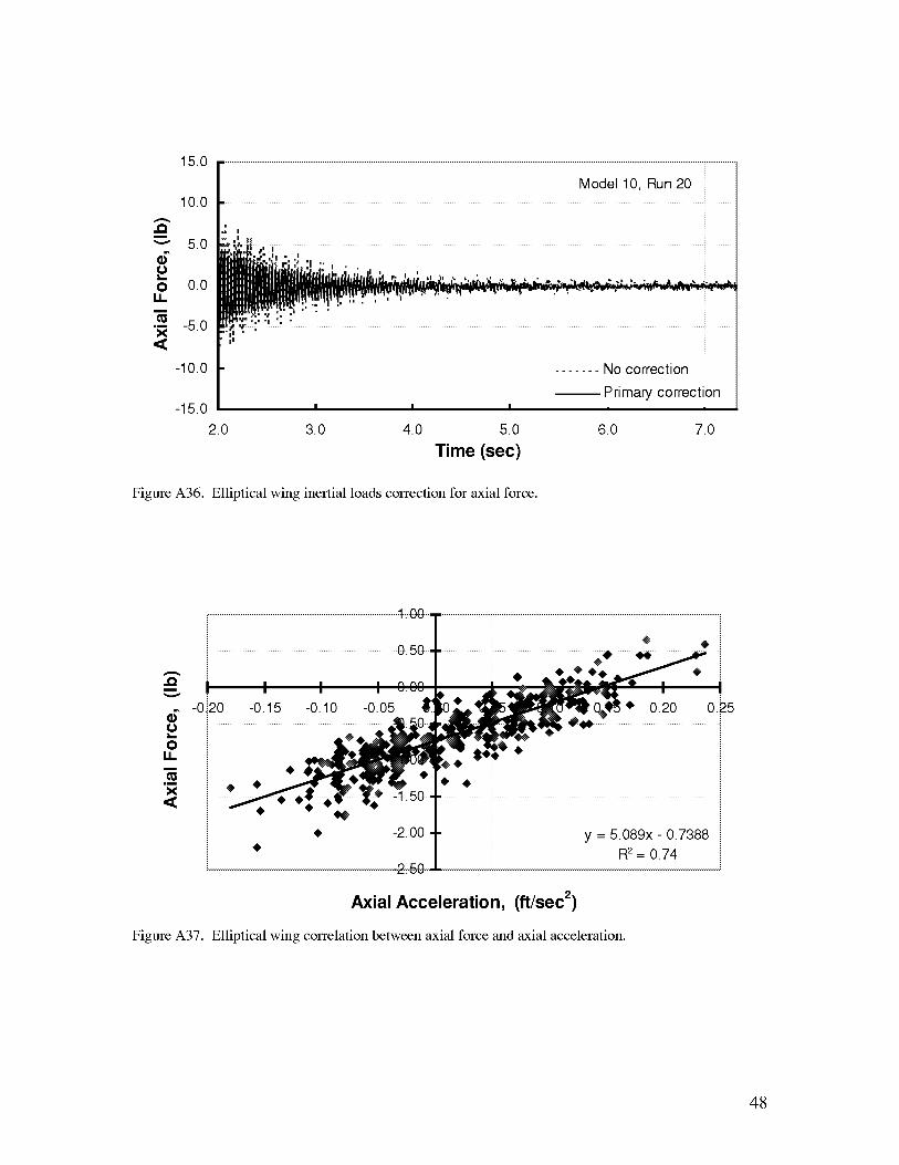
Figure A36. Elliptical wing inertial loads correction for axial force.

e',m

o"ox_

oii

,m

x,<

0:50 •

-2:O0 • y = 5.089x - 0:7388

R2 = 0.74


Figure A37. Elliptical wing correlation between axial force and axial acceleration.

48

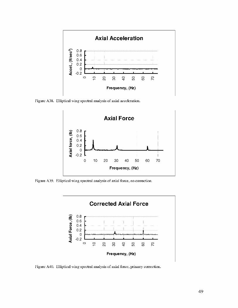
Axial Acceleration

08!iii!i 0.6

0.4

0 - -- - _.... _.... -- ----0.2-0.2

Frequency, (Hz)

Figure A38. Elliptical wing spectral analysis of axial acceleration.

Axial Force

_' 0.8

0.6oe 0.4

0.2'_ 0

-0.2

0 10 20 30 40 50 60 70

Frequency, (Hz)

Figure A39. Elliptical wing spectral analysis of axial force, no correction.

Corrected Axial Force

__' 0.8

0.6oe 0.4

,,o 0.2-- 0

_ -0.2

Frequency, (Hz)

Figure A40. Elliptical wing spectral analysis of axial force, primary correction.

49

120

,,Qm

i

'*- 60

c

Eo 0

c.m

,,c -60o

-120

Figure A41.

Mode i0 Run 20

"l_lll?,

_,_,,,,_:_1 ,,,,,, ,_._...,_ ,_

! '_ ""'1_" "_"";;;'""

....... No correction

-- Primary correctionI I I I I I I

1 2 3 4 5 6 7

Time (sec)

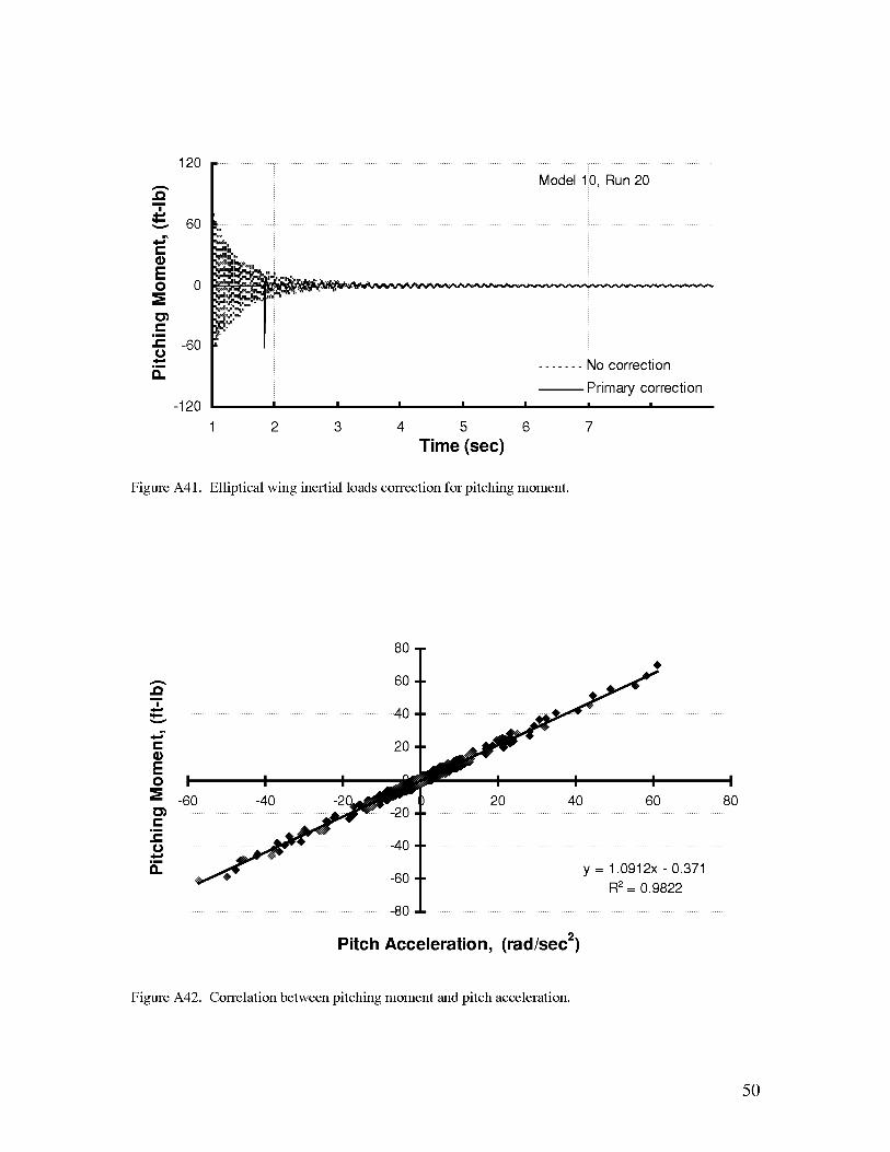
Elliptical wing inertial loads correction for pitching moment.

e',

e-

Eo

e-c-o

a.

20

I I I I I

-60 -40 -2( 20 40 60

y = 1.0912x -0.371R2= 0.9822


I

80

Figure A42. Correlation between pitching moment and pitch acceleration.

50

Pitch Acceleration

6u

u_ 4'10•_ 2

v

0utj -2 I I i I I I I

0 10 20 30 40 50 60 70

Frequency, (Hz)

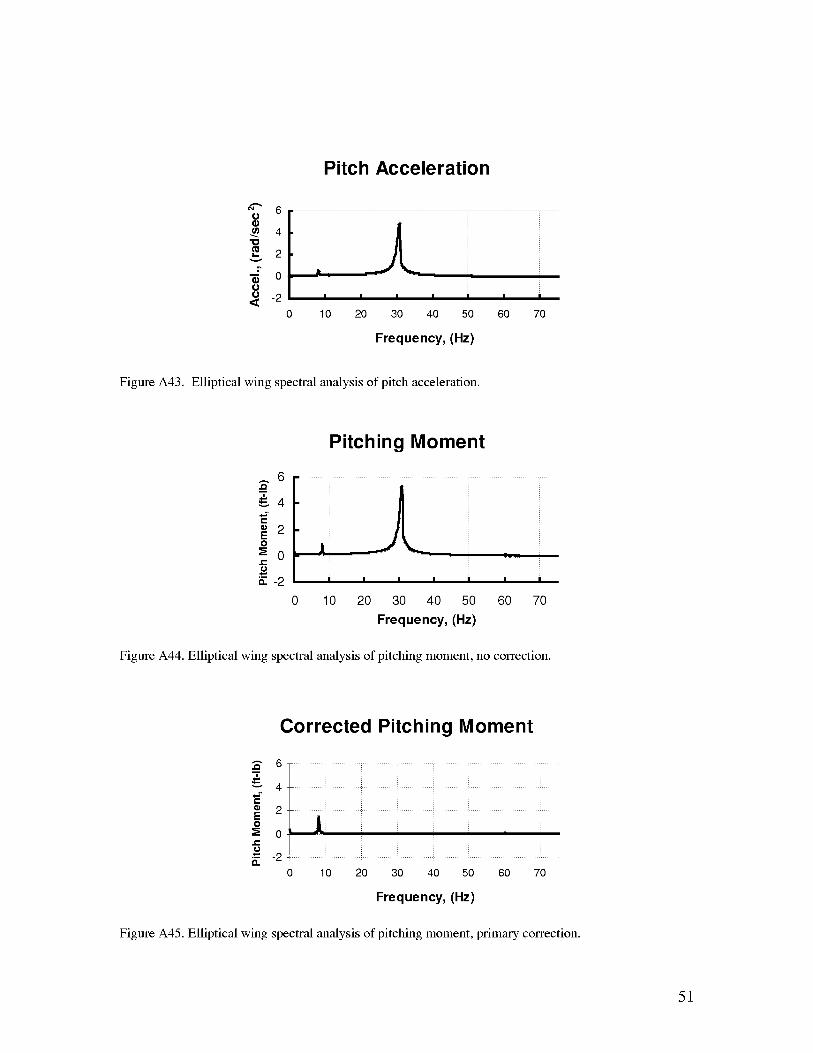
Figure A43. Elliptical wing spectral analysis of pitch acceleration.

Pitching Moment

6..Qm

&4t-"

==2O

0t'-"

E-2

0 10 20 30 40 50 60 70

Frequency, (Hz)

Figure A44. Elliptical wing spectral analysis of pitching moment, no correction.


t-"

EO

t'-"O

12.

6

4

2

o [

0 10 20 30 40 50 60 70

Frequency, (Hz)

Figure A45. Elliptical wing spectral analysis of pitching moment, primary correction.

51

APPENDIX B Post-Processing data using comboa

B.1 Logon Procedure

Enter user id:

Enter password:

dgetest

B.2 Setting up the Comboa Processing Directory

Directory: export/home/dge

Required input files: groups.pre

groups. 1422comboa

inxxx

Output files : answer

logcomboaoutcomboa

euinfo

windoff.log

B.3 Defining the inxxx file

csfile cs486

rpfile rpmamerawfile TEST46200229

229 -1 -1

YES

NO

NO

PR ALL

-1

B.3.1 rptname file

The rptname file is used to specify the parameters to be processed for each run. A report is

52

generatedfor theselectedparametersandiscalledoutcomboa.

B.4 Comboa user interface

From cmdtool window:

Type comboa

Enter Operator Input File Name: inxxxSTOP: Normal Termination of COMBOA!

53

APPENDIX C Post Processing data using dynamic

The software package dynamic performs post processing of dynamic data collected from force-

balance and accelerometer outputs. The program reads the most current answer data file created

by comboa in the same directory. The following files are required for dynamic to function:

accelr.F

dynam.F

dynamic.Fifind.F

inertia.F

mtgrt.F

lpracc.F

lprbal.F

lprsig.F

lprvel.Flinear.F

pm.F

prload.Freadd.F

rjusty.Frm.F

rmld.F

setupd.F

config6.inp

config7.inp

configl0.inp

acceleration calculations and zero offset cal from run XXX

data reduction parameters such as lift and drag coefficients

main processing unit

finds parameters in answer

performs a multivariate regression to calc moments of inertia

integrates accelerations to calculate velocities

outputs accelerations

output balance forces

output signals

output velocities

performs mass calculations

called by inertia, perfoms multivariate regression

calculates aerodynamic loadsreads answer

right justifies search field

3-component multivariate regressionsubroutine to filter the inertial loads out of the measurements

reads model configuration file

model 6 configuration file



groups.i

params.i

symfup.i

Input File

answer

Output File naming convention

runXXX_YYY_acc

runXXX_YYY_dyn

runXXX_YYY_lng

runXXX_YYY_ltd

-Accelerometer data from run Y

-Processed lift, drag coefficients, alpha, sink rate

-Longitudinal (Normal, Axial, and Pitch) loads and accelerations

-Lateral (Roll, Yaw, and Side) loads and accelerations measured

54

runXXX_YYY_ld -Velocities

runXXX_YYY_vel -Balance data in voltage form as it was acquired

runXXX_YYY_g -Accelerometer signals

The subroutine first goes through a linear regression scheme of the three force equations to

calculate the mass of the model. In these equations, m is the mass of everything on the model

side of the strain gauge of the balance. The program then uses Multivariate regression to solve

for the inertias and centroid positions involved in the three moment equations. The scheme used

for solving for these constants was to solve for the most significant terms. Therefore, Iy (y-

Inertia) in the pitching moment equation was calculated first, then Ix (x-Inertia) in the rolling

moment equation and finally Iz (z-Inertia) in the yawing moment equation. The centroid positions

were being calculated along with each of the inertias. The multivariate regression scheme has the

following form:

y= bl* xl + b2*x2 + b3*x3

where, bl, b2, b3 -regression constants (Inertias, centroid positions)

xl, x2, x3 -independent variables (acceleration data arrays)

Y -dependent variable (moment data arrays)

Once the constants are calculated, they are used to subtract the inertial loads from the total loads

in file runY.ld. The resulting residual loads are then formatted into a file which PREPLOT can

easily read. The file is composed of two zones. The first zone is the total loads and the second isthe residual loads.

Since the mass of the model, inertias and centroid positions are calculated with subroutine inertia,

cards 5 and 6 in the configuration file (configY.inp) are not necessary. However, the distances,

dist(i), from the accelerometers to the model's center of gravity will still need to be measured

since they are used in the subroutine ACCELR.

C.1 Setting up the Dynamic Processing Directory

Several model dependent configuration files are required in order to properly performcalculations:

Model 6: config6.inp

Model 7: config7.inp

Model 10: configl0.inp

55

Model configuration file

The model configuration file (configxx.inp) contains the following information:

x distance from balance moment reference center to six accelerometers (in inches)

y distfince from balance moment reference center to six accelerometers (in inches)

z distance from balance moment reference center to six accelerometers (in inches)

accelerometer sensitivities (these were configured as -1.0 if the accelerometer was placed

upside down)

mass (slugs) as calculated by the calibration runs for each model

Moments of inertia as calculated by the calibration runs for each model. (slug-f()

Wing Area (ft2) SAREA1, BSPAN1 (inches) and Reference chord length, CHORD1 (inches)


card 1 - x distance from balance to accel

2.264 2.264 3.264 14.736 15.736 16.436

card 2 y distance from balance to accel

5.5 0 0 0 0 0

card 3 z distance from balance to accel

-2.638 -2.638 -2.375 -2.638 -2.375 -2.375

card 4 x,y,z distance from balance to cg

0 0 -2.5

card 5 accel sensitivities

1.0 1.0 -1.0 1.0 1.0 1.0 1.0

card 6 mass (slugs)

1.132 1.759 1.8531

card 7 Ixx Iyy Izz Ixz slug-ft2 reference to mrc

0.6299 2.3319 2.6956 -0.001

1.0 1.0 1.0

56

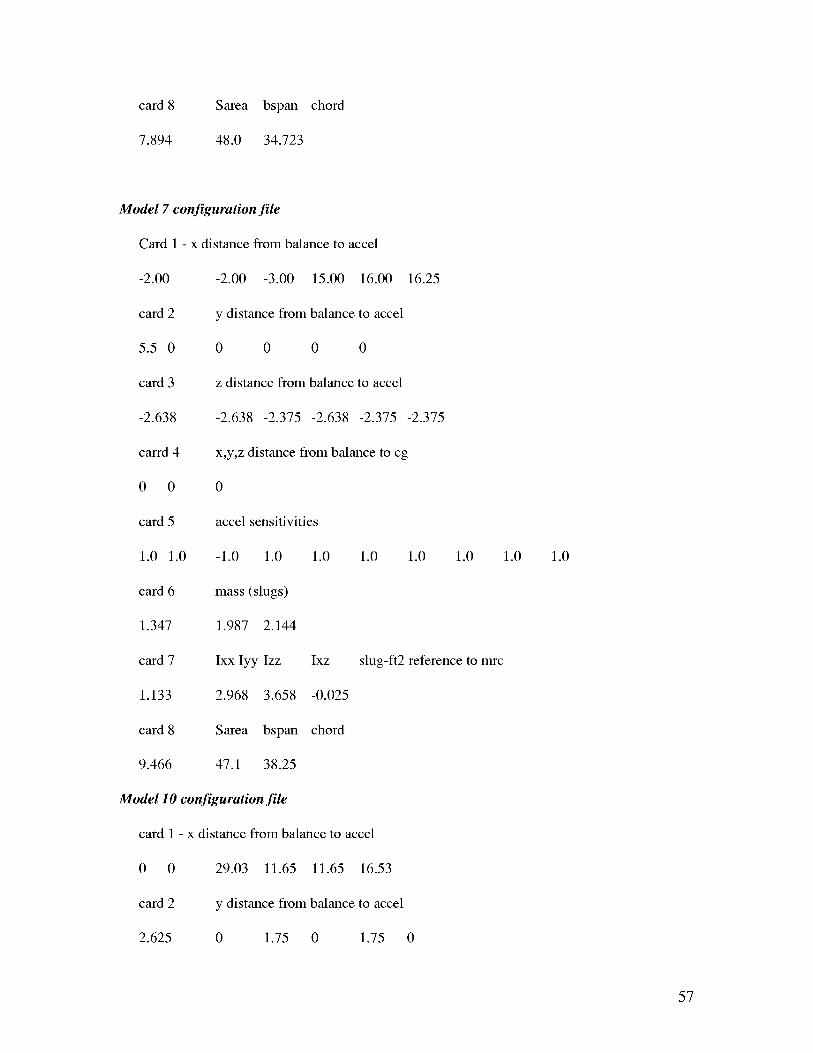
card8 Sarea bspan chord

7.894 48.0 34.723


Card 1 - x distance from balance to accel

-2.00 -2.00 -3.00 15.00 16.00 16.25


5.5 0 0 0 0 0

card 3 z distance from balance to accel

-2.638 -2.638 -2.375 -2.638 -2.375 -2.375

carrd 4 x,y,z distance from balance to cg

0 0 0

card 5 accel sensitivities

1.0 1.0 -1.0 1.0 1.0 1.0 1.0

card 6 mass (slugs)

1.347 1.987 2.144

card 7 Ixx Iyy Izz Ixz

1.133 2.968 3.658 -0.025

card 8 Sarea bspan chord

9.466 47.1 38.25


card 1 - x distance from balance to accel

0 0 29.03 11.65 11.65 16.53


2.625 0 1.75 0 1.75

1.0 1.0 1.0

slug-ft2 reference to mrc

0

57

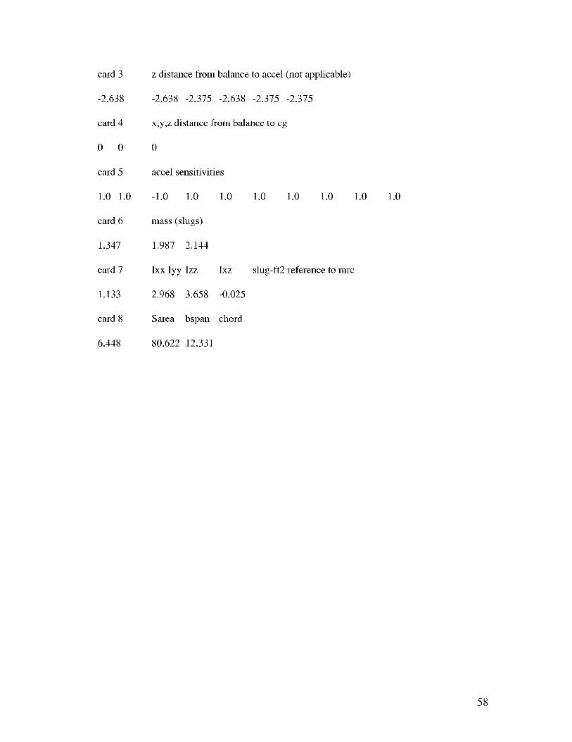
card3

-2.638

card4

0 0

card5

1.0 1.0

card6

1.347

card7

1.133

card8

6.448

zdistancefrombalancetoaccel(notapplicable)

-2.638 -2.375 -2.638 -2.375 -2.375

x,y,zdistancefrombalancetocg

0

accelsensitivities

-1.0 1.0 1.0

mass(slugs)

1.987 2.144

Ixx Iyy Izz Ixz

2.968 3.658 -0.025

Sarea bspan chord

80.62212.331

1.0 1.0 1.0 1.0 1.0

slug-ft2 reference to mrc

58

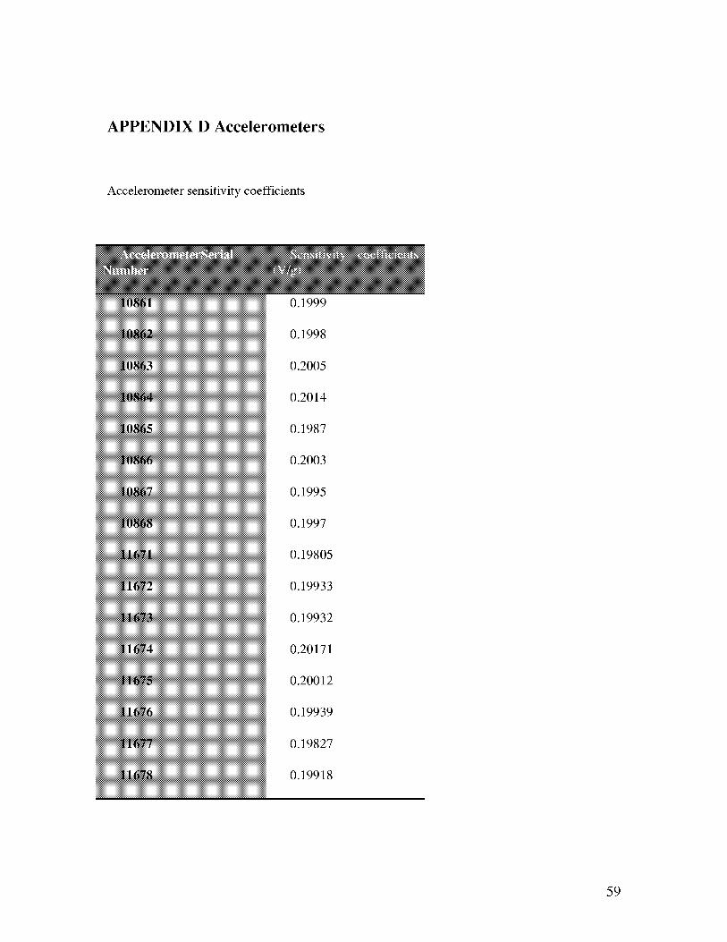
APPENDIX D Accelerometers

Accelerometer sensitivity coefficients

0.1999

0.1998

0.2005

0.2014

0.1987

0.2003

0.1995

0.1997

0.19805

0.19933

0.19932

0.20171

0.20012

0.19939

0.19827

0.19918

59

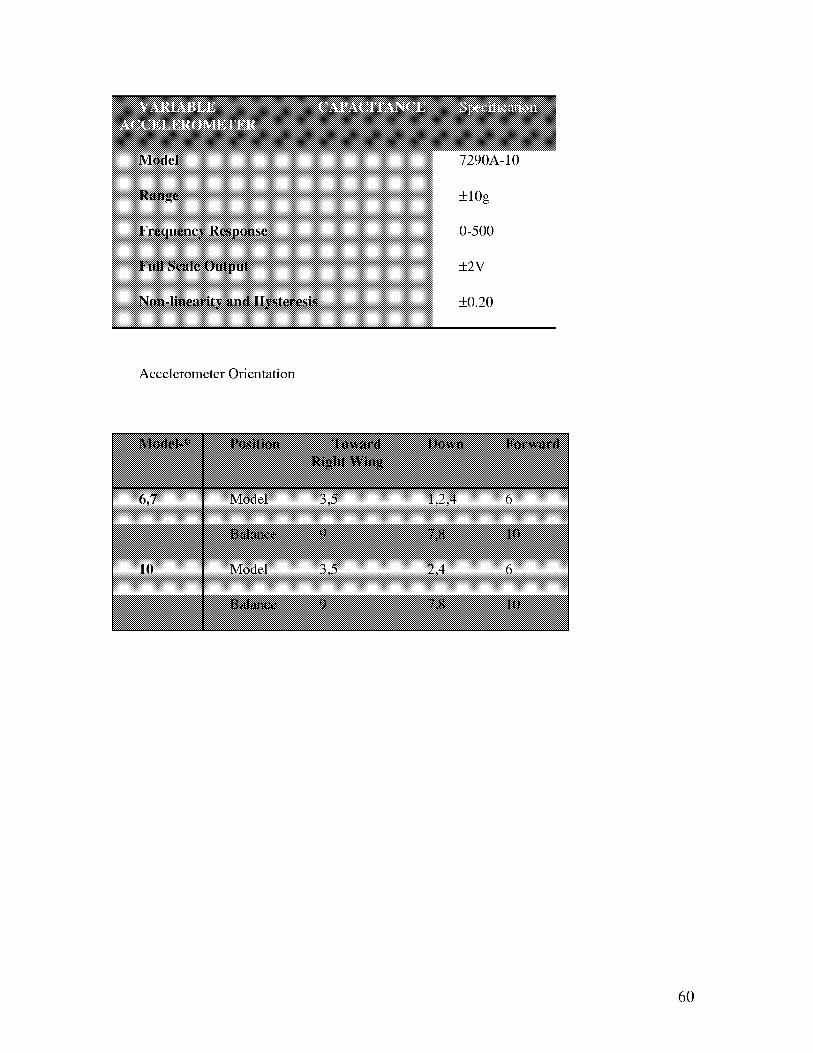
7290A-10

+10g

0-500

+2V

+0.20

Accelerometer Orientation

60

References

1 Roskam, J., Airplane Design Part VIII: Airplane Cost Estimation: Design,

Development, Manufacturing and Operating. RAEC, Ottawa, Kansas, 1990.

2 Pope, Alan, Rae, William H., Jr., Low-Speed Wind Tunnel Testing. Wiley-

Interscience, USA, 1984.

3 Kemp, W. B., Lockwood, V.E., and Phillips, W. P. "Ground Effects Related to

Landing of Airplanes with Low-Aspect Ratio Wings," NASA TN D-3583, October

1966.

4 Chang, Ray Chung, An Experimental Investigation of Dynamic Ground Effect.

University of Kansas, 1985, pp. 26.

5 Gentry, Garl L., Jr., Quinto, P. Frank, Gatlin, Gregory M., and Applin, Zachary T.,

The Langley 14- by 22- Foot Subsonic Tunnel: Description, Flow Characteristics, and

Guide for Users, NASA Technical P5.Paper 3008, September, 1990.

6 Gainer, Thomas G., Hoffman, Sherwood, Summary of Transformation Equations and

Equations of Motion Used in Free-Flight and Wind-Tunnel Data Reduction and

Analysis. NASA SP-3070, 1972, p.25.

7 Gainer, Thomas G., Hoffman, Sherwood, Summary of Transformation Equations and

Equations of Motion Used in Free Flight and Wind Turtle Data Reduction and Analysis.

NASA SP-3070, 1972, p. 57.

8 Hamming, R.W., Digital Filters, Prentice-Hall, Inc., Englewood Cliffs, New Jersey,1983.

9 Baker, Paul A., Schweikhard, William G., and Young, William R., Flight Evaluation

of Ground Effect on Several Low-Aspect Ratio Airplanes, NASA TN-D-6053, Oct1970.

10 Lee, Pai-Hung, Lan, C. Edward, and Muirhead, Vincent U., An Experimental

Investigation of Dynamic Ground Effect, NASA CR-4105, 1987.

11 Chang, Ray Chung and Muirhead, Vincent U., Effect of Sink Rate on Ground Effect

of Low-Aspect Ratio Wings, J. of Aircraft, vol. 24, no. 3, Mar 1986, pp. 176-180.

12 Kemmerly, Guy T. and Panlson, J. W., Jr., Investigation of Moving-Model

Technique for Measuring Ground Effects, NASA TM-4080, 1989.

13 Curry, Robert E., Moulton, Bryan J., and Kresse, John, An In-Flight Investigation of

Ground Effect on a Forward-Swept Wing Airplane, NASA TM-101708, Sept. 1989.

14 Corda, Stephen, Stephenson, Mark T., Burcham, Frank W., and Curry, Robert E.,

Dynamic Ground Effects Flight Test of an F-15 Aircraft, NASA TM-4604, Sept. 1994.

15 van Dam, C.P., Vijgen, P.M.H.W., and Holmes, B.J., Wind Tunnel Investigation on

the Effect of the Crescent Planform Shape on Drag, AIAA-90-0300, p. 12

16 Kemmerly, Guy T., Dynamic Ground Effect Measurements on the F-15 STOL and

Maneuver Technology Demonstrator (S/MTD) Configuration. NASA TP 3000, 1987.

61

REPORT DOCUMENTATION PAGE Form ApprovedOMB No. 0704-0188

Public reporting burden for this collection of information is estimated to average 1 hour per response, including the time for reviewing instructions, searching existing datasources, gathering and maintaining the data needed, and completing and reviewing the collection of information. Send comments regarding this burden estimate or any otheraspect of this collection of information, including suggestions for reducing this burden, to Washington Headquarters Services, Directorate for Information Operations andReports, 1215 Jefferson DavisHighway,Suite12_4,Ar_ingt_n,VA222_2-43_2,andt_the__ice_fManagementandBudget,Paperw_rkReducti_nPr_ject(_7_4-_188),Washington, DC 20503.

1. AGENCY USE ONLY (Leave blank) 2. REPORT DATE 3. REPORT TYPE AND DATES COVERED

August 1999 Contractor Report

4. TITLE AND SUBTITLE 5. FUNDING NUMBERS

Investigation of a Technique for Measuring Dynamic Ground Effect in aSubsonic Wind Tunnel NCC1-24

6. AUTHOR(S)Sharon S. Graves

7. PERFORMING ORGANIZATION NAME(S) AND ADDRESS(ES)


Joint Institute for Advancement of Flight SciencesLangley Research Center, Hampton, Virginia 23681-2199

9. SPONSORING/MONITORING AGENCY NAME(S) AND ADDRESS(ES)

National Aeronautics and Space AdministrationNASA Langley Research CenterHampton, VA 23681-2199

537-07-51-02

8. PERFORMING ORGANIZATION

REPORT NUMBER

10. SPONSORING/MONITORING

AGENCY REPORT NUMBER

NASA/CR- 1999 -209544

11. SUPPLEMENTARY NOTES

Graves: Graduate Research Scholar Assistatant, GW JIAFS. This research was conducted in partial satisfactionof the requirements for the degree of Master of Science with The George Washington University.

Langley Technical Monitor: Edgar G. Waggoner12a. DISTRIBUTION/AVAILABILITY STATEMENT

Unclassified-Unlimited

Subject Category 02 Distribution: Nonstandard

Availability: NASA CASI (301) 621-0390

12b. DISTRIBUTION CODE

13. ABSTRACT (Maximum 200 words)

To better understand the ground effect encountered by slender wing supersonic transport aircraft, a test wasconducted at NASA Langley Research Center's 14 x 22 foot Subsonic Wind Tunnel in October, 1997.Emphasis was placed on improving the accuracy of the ground effect data by using a "dynamic" technique inwhich the model's vertical motion was varied automatically during wind-on testing. This report describes andevaluates different aspects of the dynamic method utilized for obtaining ground effect data in this test. Themethod for acquiring and processing time data from a dynamic ground effect wind tunnel test is outlined withdetails of the overall data acquisition system and software used for the data analysis. The removal of inertial

loads due to sting motion and the support dynamics in the balance force and moment data measurements of theaerodynamic forces on the model is described. An evaluation of the results identifies problem areas providingrecommendations for future experiments. Test results are validated by comparing test data for an elliptical wingplanform with an Elliptical wing planform section with a NACA 0012 airfoil to results found in currentliterature. Major aerodynamic forces acting on the model in terms of lift curves for determining ground effectare presented. Comparisons of flight and wind tunnel data for the TU-144 are presented.

14. SUBJECT TERMS

Dynamic Ground Effect; Subsonic Wind Tunnel Test; Data Acquisition System

17. SECURITY CLASSIFICATION

OF REPORT

Unclassified


OF THIS PAGE

Unclassified


OF ABSTRACT

Unclassified

15. NUMBER OF PAGES

66

16. PRICE CODE

A04

20. LIMITATION

OF ABSTRACT

NSN 7540-01-280-5500 Standard Form 298 (Rev. 2-89)

Prescribed by ANSI Std. Z-39-18298-102

Documents

Investigation of a Technique for Measuring Dynamic Ground ... · Investigation of a Technique for Measuring Dynamic Ground Effect in a ... Investigation of a Technique for Measuring