1

Measuring spatial clustering in disease patterns.

Peter Congdon, Queen Mary University of Londonp.congdon@qmul.ac.uk

http://www.geog.qmul.ac.uk/staff/congdonp.htmlhttp://webspace.qmul.ac.uk/pcongdon/

2

Background: spatial principles and spatial correlation

Tobler’s First Law of Geography: “All places are related but nearby places are more related than distant places”

Spatial correlation (similar values in nearby spatial units) a common feature of geographic datasets (spatial econometrics, area health, political science etc).

Can have positive or negative correlation, but positive correlation most common

So spatial correlation indices measure correlation but also account for distance between spatial units (including spatial contiguity)

Reference (null) pattern: spatial randomness. Values observed at one location do not depend on values observed at neighboring locations

3

Background: spatial principles and spatial heterogeneity

Michael Goodchild in “Challenges in geographical information science”, Proc RSA 2011” mentions also a second empirical principle: spatial heterogeneity.

In fact, an example of such heterogeneity is local variation in the degree of spatial dependence, leading to local indices of spatial association

4

Background: observation types

My focus is on spatial lattice data: N areal subdivisions (e.g. administrative areas) which taken together constitute the entire study region.

Unlike point data (geostatistics), where major focus is on interpolating a response between observed locations.

5

Global Indices of Spatial Association

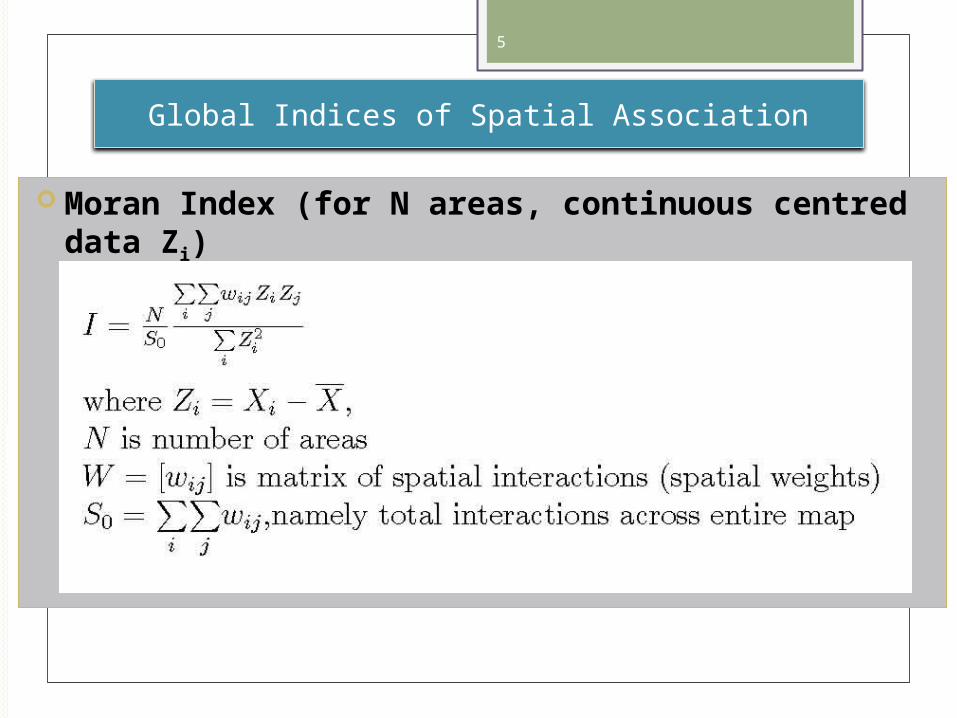
Moran Index (for N areas, continuous centred data Zi)

6

Spatial Weights

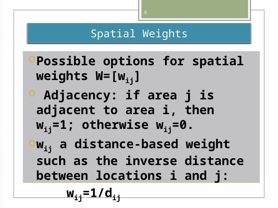
Possible options for spatial weights W=[wij]

Adjacency: if area j is adjacent to area i, then wij=1; otherwise wij=0.

wij a distance-based weight such as the inverse distance between locations i and j: wij=1/dij

7

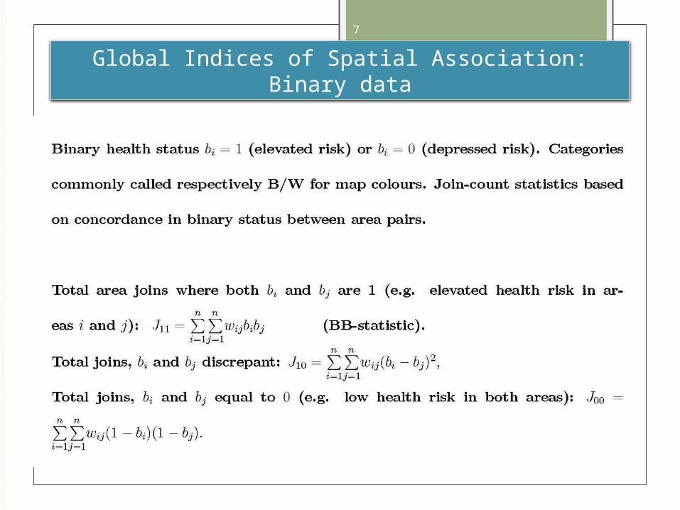
Global Indices of Spatial Association: Binary data

8

Background: Area health data and spatial correlation

Health data with full population coverage (as opposed to survey data) often only available for geographic aggregates.

These may be small neighbourhoods, such as English lower super output areas (LSOAs). Average 1500-2000 population.

Small area units (with homogenous social structure, environment and other exposures) preferable for reducing ecologic bias

9

Background: Area health data and spatial correlation

Examples of area health data (e.g. for electoral wards, LSOAs): mortality data by cause, cancer incidence data, health prevalence data

Spatial correlation in area health outcomes reflects clustering in risk factors (observed and unobserved), such as deprivation/affluence, health behaviours, environmental factors, neighbourhood social capital

10

Bayesian Relative Risk Models for Area Spatial Data

Bayesian models for area disease risks now widely applied (to detect smooth underlying risk surface over space, etc).

Assume observed disease counts yi Poisson distributed,

yi ~Po(eiri), (ei = expected counts) Relative risks ri have average 1 when

sum(expected)=sum(observed). Expected counts (demographic sense) based on applying region-wide disease rates to each small area population

11

Bayesian Relative Risk Models for Area Spatial Data

One option for modelling area relative risks, convolution scheme (Besag et al, 1991) log(ri)=+si+ui, Spatial error: si~Conditional Autogressive (CAR)

Heterogeneity/overdispersion error: ui ~ Unstructured White Noise

12

Neighbourhood Clustering in Elevated Risk

Consider binary risk measures: bi=1 if relative risk ri>1, bi=0 otherwise. This is latent (unknown) as ri is latent.

Can use other thresholds (e.g. ri>1.5) Interest often in posterior exceedance

probabilities of elevated disease risk Ei=Pr(ri>1|y)=Prob(bi=1|y)

in each area separately. Possible rules: area i a hotspot if Ei > 0.9 or

if Ei>0.8. Suitable threshold may depend on data frequency

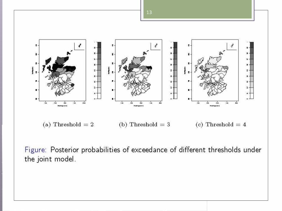
13

14

Neighbourhood Clustering in Elevated Risk

“Hotspot” detection does not measure broader local clustering in relative risks.

High risk clustering: (a) area i embedded in high risk cluster

(aka, high risk cluster centre) both area i and all surrounding areas j have elevated risk, (Ei and Ej both high).

(b) High risk outlier or high risk cluster edge: high risk area i (Ei high), but all or majority of adjacent areas j are low risk (Ej low)

15

Neighbourhood Clustering in Elevated Risk

Low risk clustering:(c) area i embedded in low risk

cluster: both area i and surrounding areas have low risk (Ei and Ej both low) .

(d) low risk outlier or low risk cluster edge: low risk area (Ei

low) but all or many adjacent areas are high risk

16

Spatial Scan Clusters

Most well known approach based on spatial scan method: produces lists of areas in a cluster at given significance, e.g. under Poisson model for {yi,ei} data

Spatial scan: circle (or ellipse) of varying size systematically scans the study region (moving window).

Each geographic unit (e.g. census tract) is a potential cluster centre.

Clusters are reported for those circles where observed values within circle are greater than expected values.

17

Stochastic Approach to Measuring Clustering in Elevated Risk

Method to be described provides measure of cluster status for each area in situation where relative health risks ri (and health status bi) are unknowns

Can be considered a method of cluster detection, included in MCMC updating

Encompasses high risk and low risk clustering and also outliers (isolated high or low risk hotspot)

18

Synthetic Data

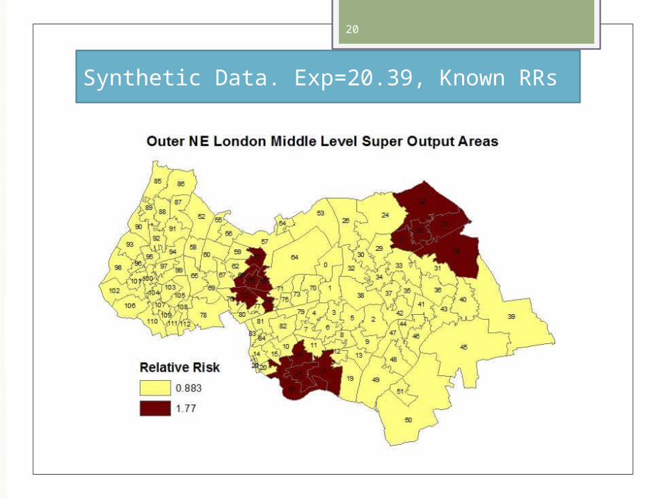
Known adjacency structure: 113 middle level super output areas (MSOAs) in Outer NE London

15 out of 113 areas have high RR (ri circa 1.75). Remainder have below average RR (ri circa 0.9).

High risk areas are located in three high risk clusters

Known yi and ei, and hence known crude relative risks, but whether RRs significantly elevated or not depends on information in data

19

Synthetic Data

Assess Ei and bi (using convolution model) according to different expected cases: ei=20.39, or ei=58.77.

For ei=20.39, yi are either 18 or 36 (to ensure sum of observed and expected are the same)

For ei=58.77, yi are either 52 or 103

20

Synthetic Data. Exp=20.39, Known RRs

21

How to Detect Clustering in Relative Disease Risk: Local Join-Counts

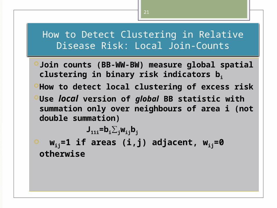
Join counts (BB-WW-BW) measure global spatial clustering in binary risk indicators bi

How to detect local clustering of excess risk Use local version of global BB statistic with

summation only over neighbours of area i (not double summation)

J11i=bi∑jwijbj

wij=1 if areas (i,j) adjacent, wij=0 otherwise

22

Local Join-Counts to describe local clustering

J11i measures high risk “cluster embeddedness”

J11i will be high for areas surrounded by other high risk areas

i.e. when area i and all/most neighbours j both have high risk.

23

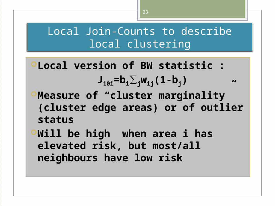
Local Join-Counts to describe local clustering

Local version of BW statistic : J10i=bi∑jwij(1-bj)Measure of “cluster marginality”

(cluster edge areas) or of outlier status

Will be high when area i has elevated risk, but most/all neighbours have low risk

24

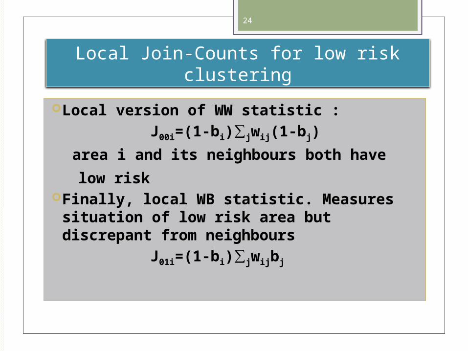
Local Join-Counts for low risk clustering

Local version of WW statistic : J00i=(1-bi)∑jwij(1-bj)

area i and its neighbours both have

low riskFinally, local WB statistic. Measures

situation of low risk area but discrepant from neighbours

J01i=(1-bi)∑jwijbj

25

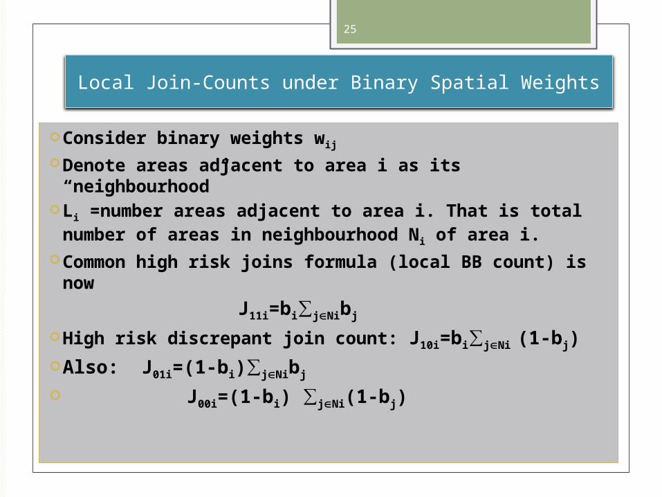
Local Join-Counts under Binary Spatial Weights

Consider binary weights wij Denote areas adjacent to area i as its

“neighbourhood” Li =number areas adjacent to area i. That is total

number of areas in neighbourhood Ni of area i. Common high risk joins formula (local BB count) is

now

J11i=bi∑jNibj

High risk discrepant join count: J10i=bi∑jNi (1-bj) Also: J01i=(1-bi)∑jNibj

J00i=(1-bi) ∑jNi(1-bj)

26

Local Join-Counts under Binary Spatial Weights

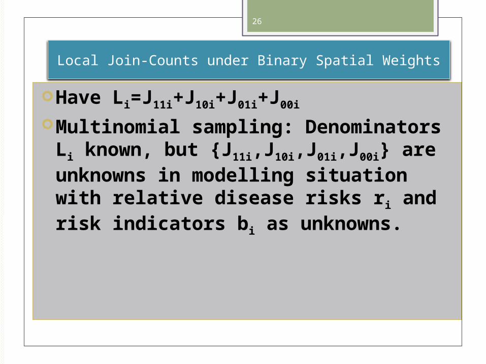
Have Li=J11i+J10i+J01i+J00i

Multinomial sampling: Denominators Li known, but {J11i,J10i,J01i,J00i} are unknowns in modelling situation with relative disease risks ri and risk indicators bi as unknowns.

27

Probabilities of Local Clustering

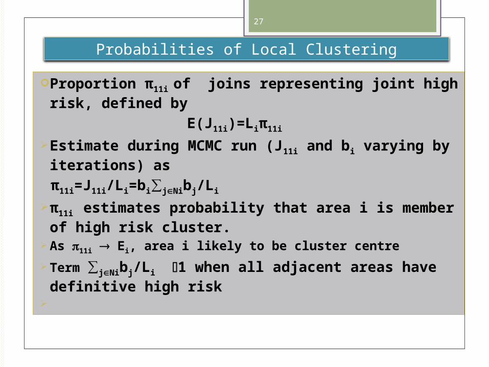
Proportion π11i of joins representing joint high risk, defined by

E(J11i)=Liπ11i

Estimate during MCMC run (J11i and bi varying by iterations) as

π11i=J11i/Li=bi∑jNibj/Li

π11i estimates probability that area i is member of high risk cluster.

As 11i Ei, area i likely to be cluster centre

Term ∑jNibj/Li 1 when all adjacent areas have definitive high risk

28

Probabilities of Local Clustering

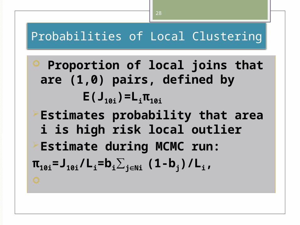
Proportion of local joins that are (1,0) pairs, defined by

E(J10i)=Liπ10i

Estimates probability that area i is high risk local outlier

Estimate during MCMC run: π10i=J10i/Li=bi∑jNi (1-bj)/Li,

29

Decomposition of Exceedance Probability

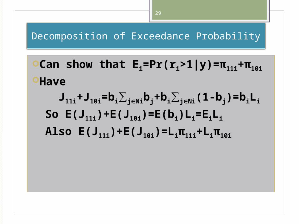
Can show that Ei=Pr(ri>1|y)=π11i+π10i

Have J11i+J10i=bi∑jNibj+bi∑jNi(1-bj)=biLi

So E(J11i)+E(J10i)=E(bi)Li=EiLi

Also E(J11i)+E(J10i)=Liπ11i+Liπ10i

30

Synthetic Data Example: Cluster Focus

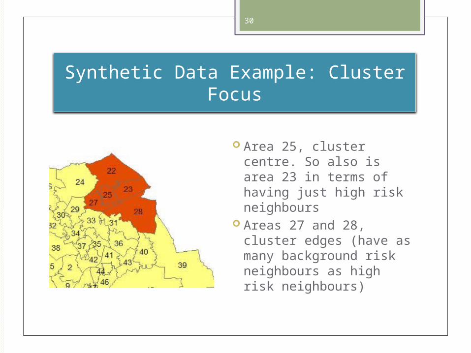
Area 25, cluster centre. So also is area 23 in terms of having just high risk neighbours

Areas 27 and 28, cluster edges (have as many background risk neighbours as high risk neighbours)

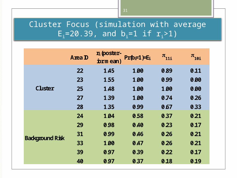
31

Cluster Focus (simulation with average Ei=20.39, and bi=1 if ri>1)

Area IDri (poster-ior mean)

Pr(bi=1)=Ei p11i p10i

22 1.45 1.00 0.89 0.11

23 1.55 1.00 0.99 0.00

25 1.48 1.00 1.00 0.00

27 1.39 1.00 0.74 0.26

28 1.35 0.99 0.67 0.33

24 1.04 0.58 0.37 0.21

29 0.98 0.40 0.23 0.17

31 0.99 0.46 0.26 0.21

33 1.00 0.47 0.26 0.21

39 0.97 0.39 0.22 0.17

40 0.97 0.37 0.18 0.19

Cluster

Background Risk

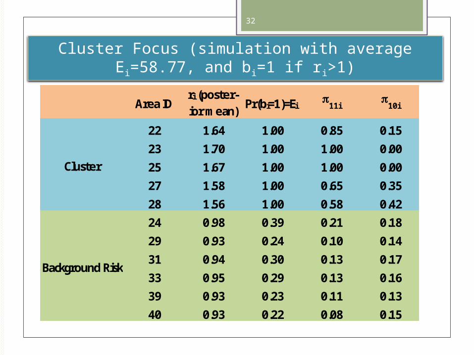
32

Cluster Focus (simulation with average Ei=58.77, and bi=1 if ri>1)

Area IDri (poster-ior mean)

Pr(bi=1)=Ei p11i p10i

22 1.64 1.00 0.85 0.15

23 1.70 1.00 1.00 0.00

25 1.67 1.00 1.00 0.00

27 1.58 1.00 0.65 0.35

28 1.56 1.00 0.58 0.42

24 0.98 0.39 0.21 0.18

29 0.93 0.24 0.10 0.14

31 0.94 0.30 0.13 0.17

33 0.95 0.29 0.13 0.16

39 0.93 0.23 0.11 0.13

40 0.93 0.22 0.08 0.15

Cluster

Background Risk

33

Cluster Centres and Edges

Cluster centre status verified: 11i Ei for areas 25 and 23.

Cluster edge status becomes clearer with more frequent data (for areas 27 and 28)

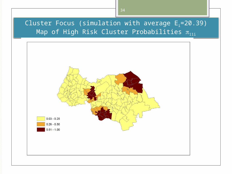
34

Cluster Focus (simulation with average Ei=20.39)Map of High Risk Cluster Probabilities 11i

35

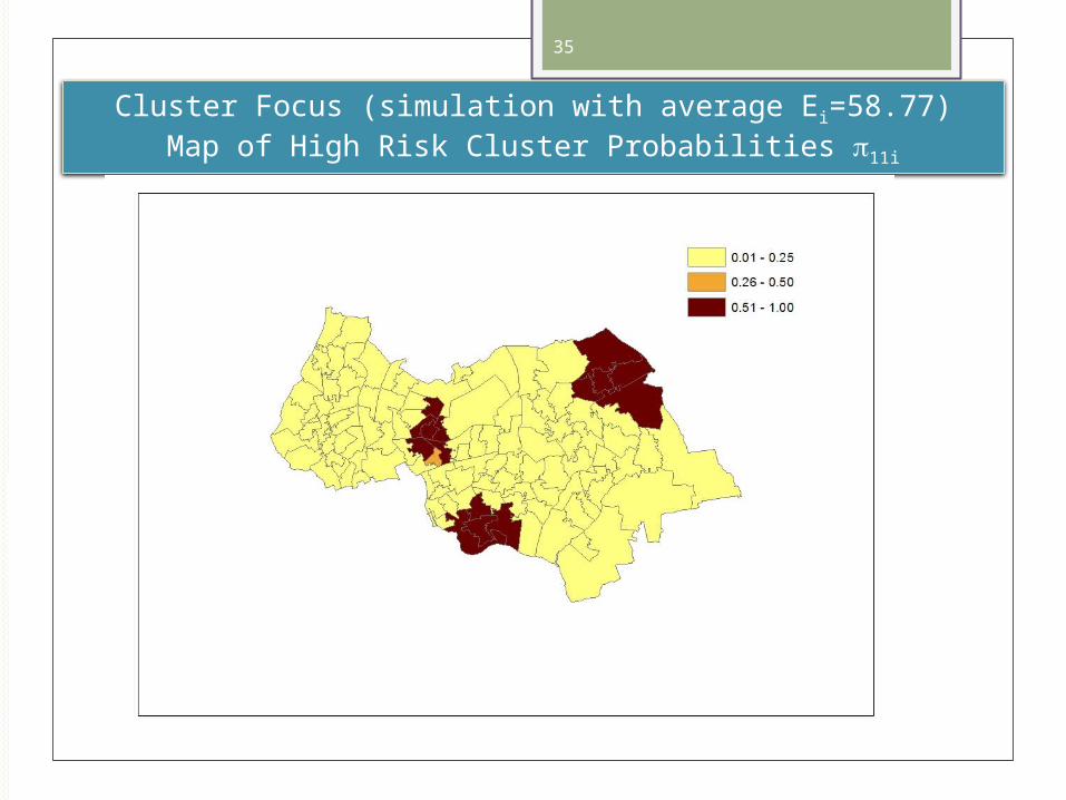
Cluster Focus (simulation with average Ei=58.77)Map of High Risk Cluster Probabilities 11i

36

Another simulation where clustering pattern known: cluster centre status under uneven risk scenario

Performance of 11i for measuring cluster centre status for contrasting situations

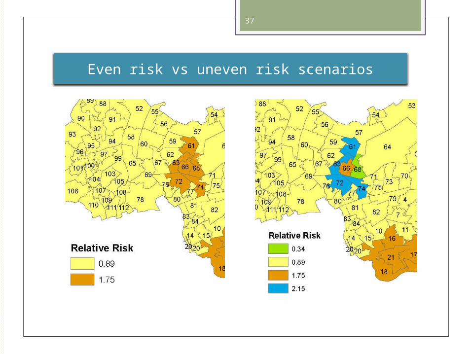
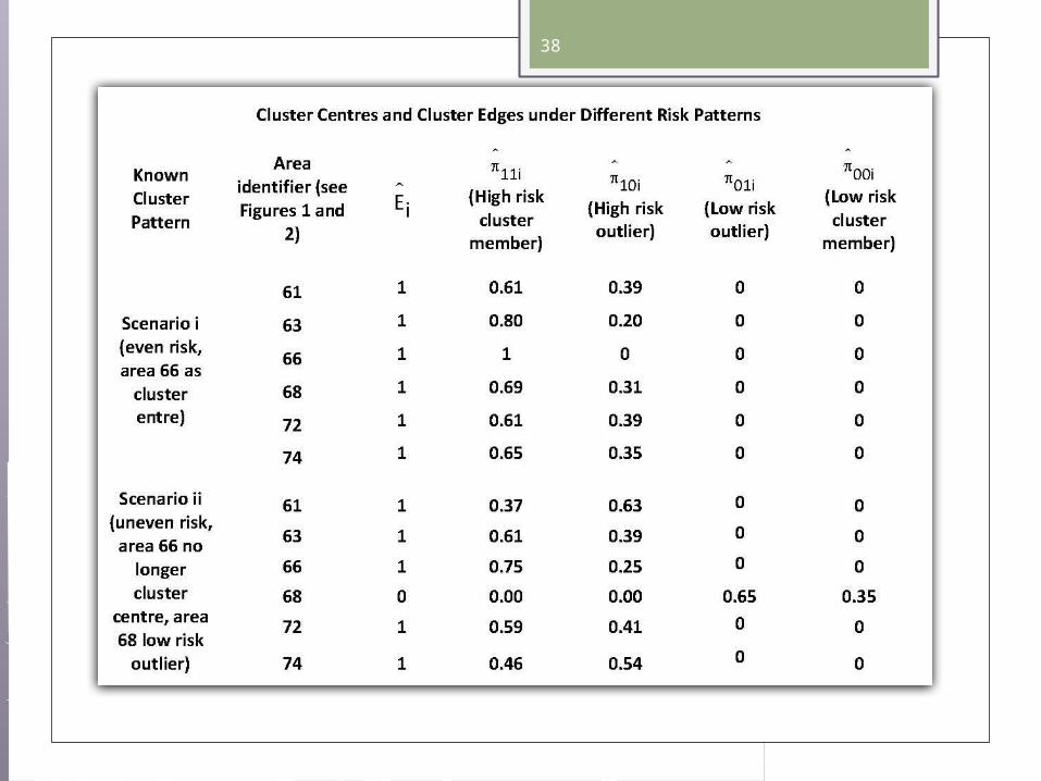
(1) EVEN RISK. High risk characterises all neighbours surrounding area i (so area i is cluster centre), and risk evenly distributed among neighbors

(2) UNEVEN RISK. High risk is not common to all neighbours, but unevenly concentrated among a few neighbors, so area i is no longer a cluster centre, and possibly a cluster edge.

37

Even risk vs uneven risk scenarios

38

39

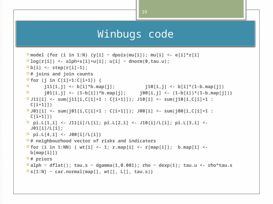
Winbugs code

model {for (i in 1:N) {y[i] ~ dpois(mu[i]); mu[i] <- e[i]*r[i] log(r[i]) <- alph+s[i]+u[i]; u[i] ~ dnorm(0,tau.u); b[i] <- step(r[i]-1); # joins and join counts for (j in C[i]+1:C[i+1]) { j11[i,j] <- b[i]*b.map[j]; j10[i,j] <- b[i]*(1-b.map[j]) j01[i,j] <- (1-b[i])*b.map[j]; j00[i,j] <- (1-b[i])*(1-b.map[j])} J11[i] <- sum(j11[i,C[i]+1 : C[i+1]]); J10[i] <- sum(j10[i,C[i]+1 : C[i+1]]) J01[i] <- sum(j01[i,C[i]+1 : C[i+1]]); J00[i] <- sum(j00[i,C[i]+1 : C[i+1]]) pi.L[1,i] <- J11[i]/L[i]; pi.L[2,i] <- J10[i]/L[i]; pi.L[3,i] <- J01[i]/L[i]; pi.L[4,i] <- J00[i]/L[i]} # neighbourhood vector of risks and indicators for (i in 1:NN) { wt[i] <- 1; r.map[i] <- r[map[i]]; b.map[i] <- b[map[i]]} # priors alph ~ dflat(); tau.s ~ dgamma(1,0.001); rho ~ dexp(1); tau.u <-

rho*tau.s s[1:N] ~ car.normal(map[], wt[], L[], tau.s)}

40

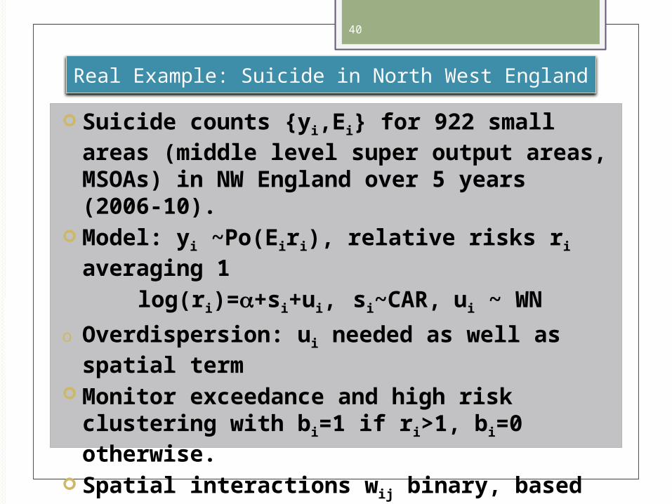
Real Example: Suicide in North West England

Suicide counts {yi,Ei} for 922 small areas (middle level super output areas, MSOAs) in NW England over 5 years (2006-10).

Model: yi ~Po(Eiri), relative risks ri averaging 1 log(ri)=+si+ui, si~CAR, ui ~ WN

o Overdispersion: ui needed as well as spatial term

Monitor exceedance and high risk clustering with bi=1 if ri>1, bi=0 otherwise.

Spatial interactions wij binary, based on adjacency

41

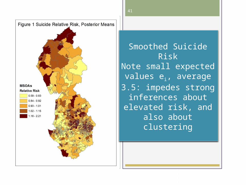
Smoothed Suicide Risk

Note small expected values ei, average

3.5: impedes strong inferences about elevated risk, and

also about clustering

42

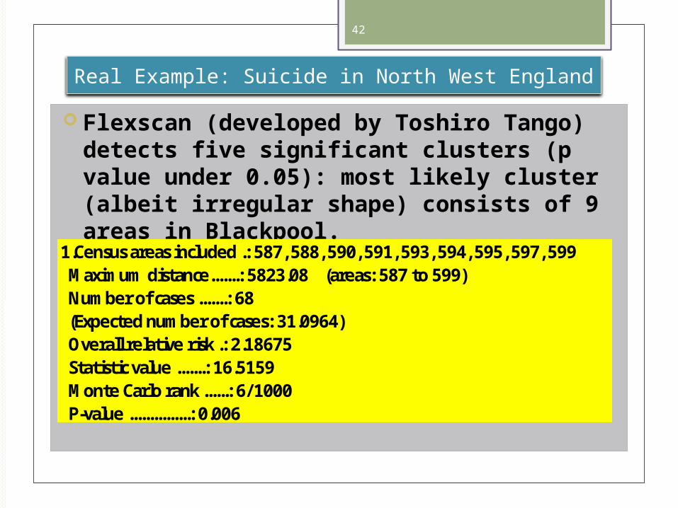
Real Example: Suicide in North West England

Flexscan (developed by Toshiro Tango) detects five significant clusters (p value under 0.05): most likely cluster (albeit irregular shape) consists of 9 areas in Blackpool.

1.Census areas included .: 587, 588, 590, 591, 593, 594, 595, 597, 599 Maximum distance.......: 5823.08 (areas: 587 to 599) Number of cases .......: 68 (Expected number of cases: 31.0964) Overall relative risk .: 2.18675 Statistic value .......: 16.5159 Monte Carlo rank ......: 6/1000 P-value ...............: 0.006

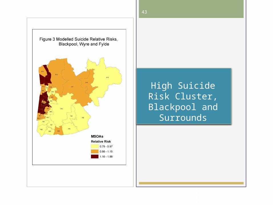
43

High Suicide Risk Cluster, Blackpool

and Surrounds

44

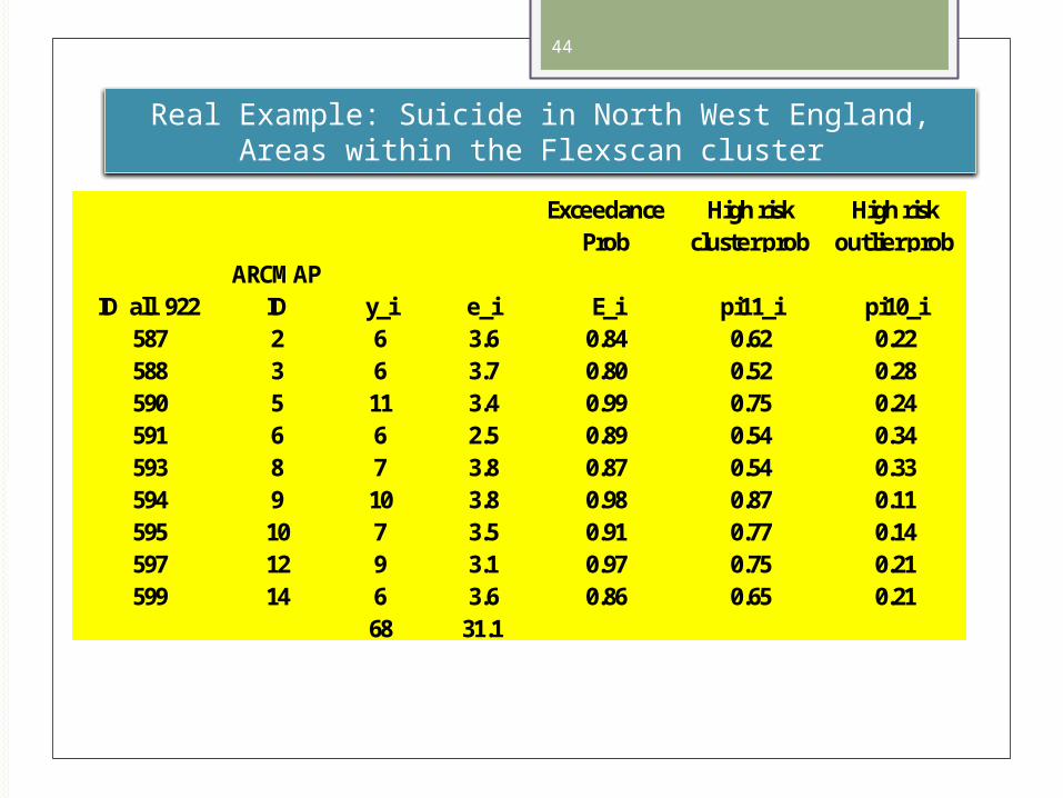
Real Example: Suicide in North West England, Areas within the Flexscan cluster

Exceedance Prob

High risk cluster prob

High risk outlier prob

ID_all_922ARCMAP

ID y_i e_i E_i pi11_i pi10_i587 2 6 3.6 0.84 0.62 0.22588 3 6 3.7 0.80 0.52 0.28590 5 11 3.4 0.99 0.75 0.24591 6 6 2.5 0.89 0.54 0.34593 8 7 3.8 0.87 0.54 0.33594 9 10 3.8 0.98 0.87 0.11595 10 7 3.5 0.91 0.77 0.14597 12 9 3.1 0.97 0.75 0.21599 14 6 3.6 0.86 0.65 0.21

68 31.1

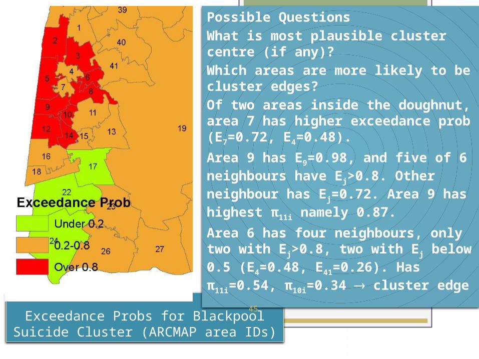
45Exceedance Probs for Blackpool Suicide

Cluster (ARCMAP area IDs)

Possible QuestionsWhat is most plausible cluster centre (if any)?Which areas are more likely to be cluster edges?Of two areas inside the doughnut, area 7 has higher exceedance prob (E7=0.72, E4=0.48).

Area 9 has E9=0.98, and five of 6 neighbours have Ej>0.8. Other neighbour has Ej=0.72. Area 9 has highest π11i namely 0.87.

Area 6 has four neighbours, only two with Ej>0.8, two with Ej below 0.5 (E4=0.48, E41=0.26). Has π11i=0.54, π10i=0.34 cluster edge

46

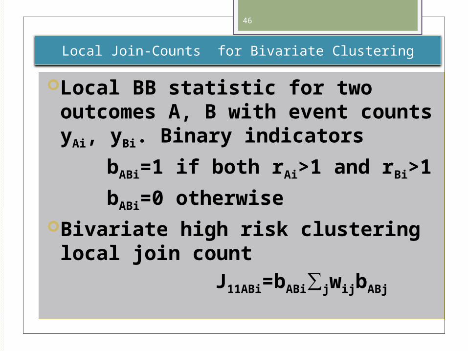
Local Join-Counts for Bivariate Clustering

Local BB statistic for two outcomes A, B with event counts yAi, yBi. Binary indicators

bABi=1 if both rAi>1 and rBi>1

bABi=0 otherwiseBivariate high risk clustering local join count

J11ABi=bABi∑jwijbABj

47

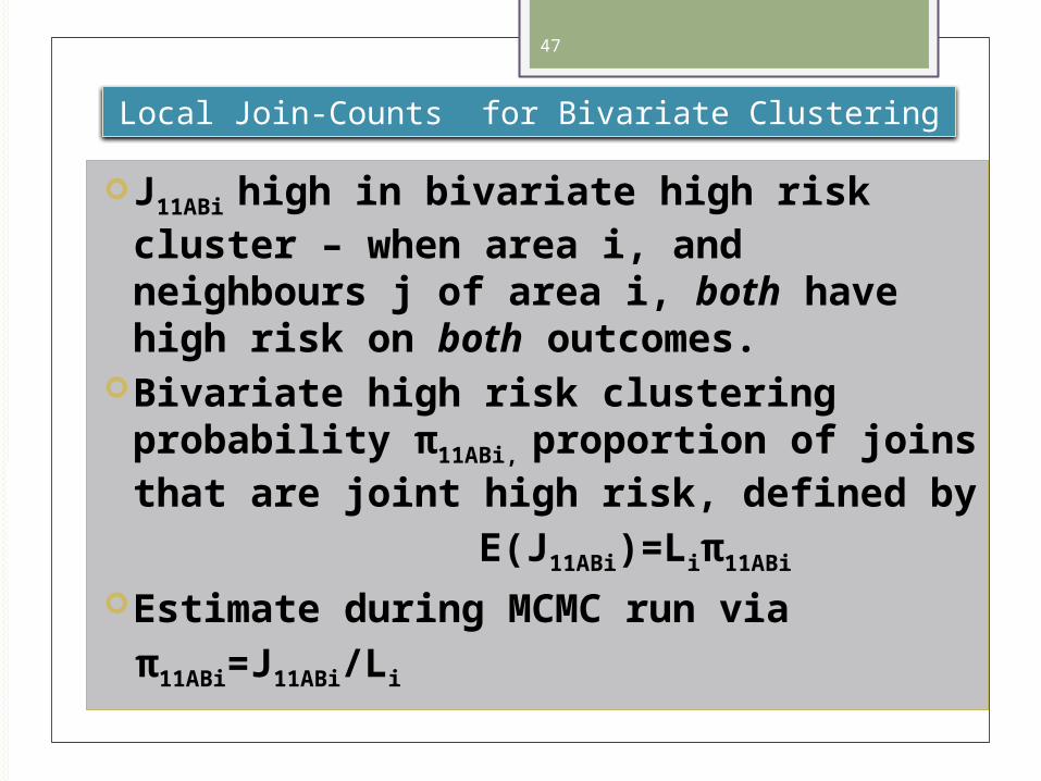
Local Join-Counts for Bivariate Clustering

J11ABi high in bivariate high risk cluster – when area i, and neighbours j of area i, both have high risk on both outcomes.

Bivariate high risk clustering probability π11ABi, proportion of joins that are joint high risk, defined by

E(J11ABi)=Liπ11ABi

Estimate during MCMC run viaπ11ABi=J11ABi/Li

48

Two outcomes: Likelihood and Prior

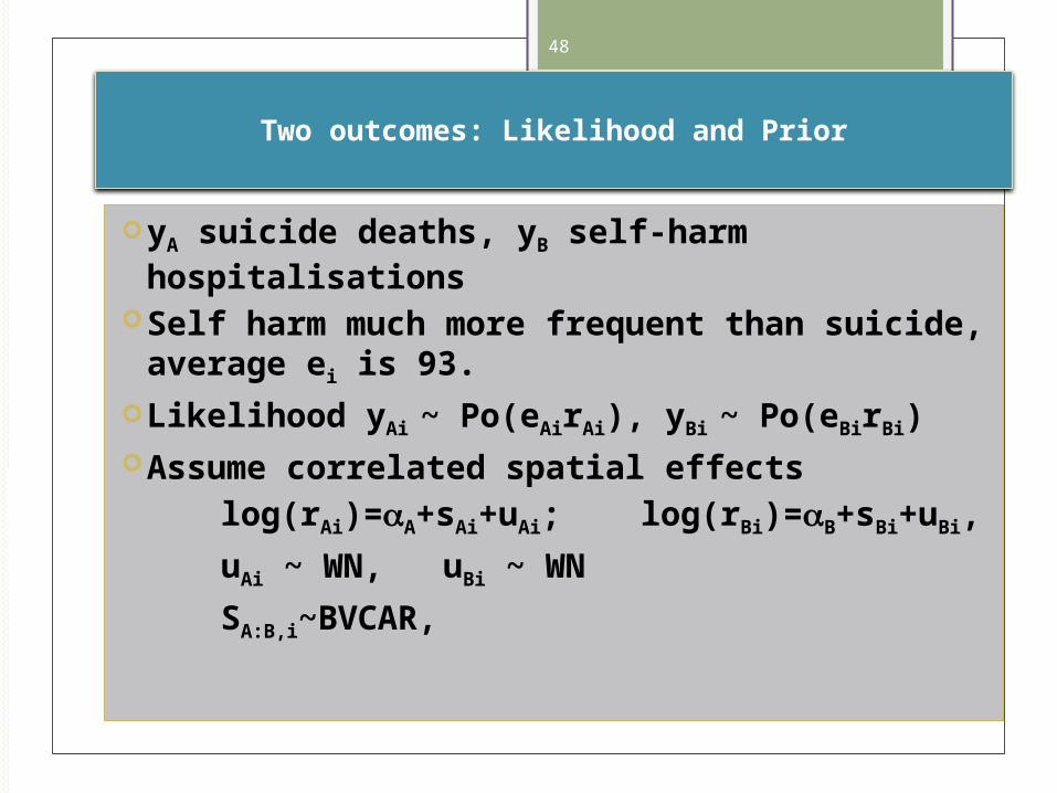
yA suicide deaths, yB self-harm hospitalisations

Self harm much more frequent than suicide, average ei is 93.

Likelihood yAi ~ Po(eAirAi), yBi ~ Po(eBirBi) Assume correlated spatial effects log(rAi)=A+sAi+uAi; log(rBi)=B+sBi+uBi,

uAi ~ WN, uBi ~ WN

SA:B,i~BVCAR,

49

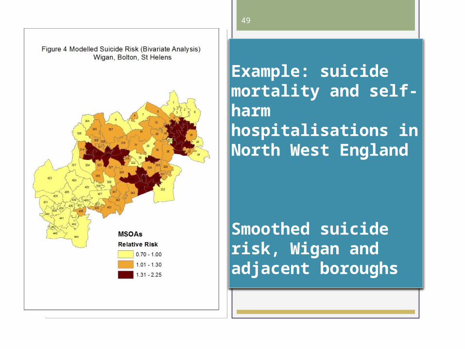
Example: suicide mortality and self-harm hospitalisations in North West England

Smoothed suicide risk, Wigan and adjacent boroughs

50

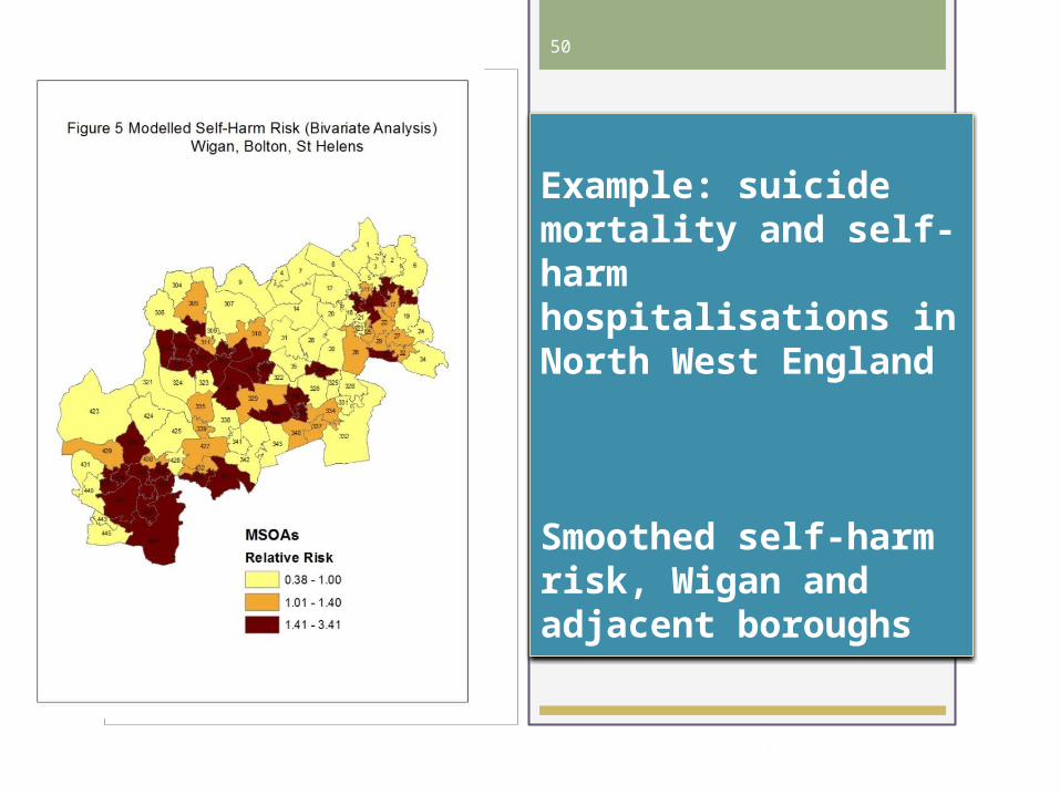
Example: suicide mortality and self-harm hospitalisations in North West England

Smoothed self-harm risk, Wigan and adjacent boroughs

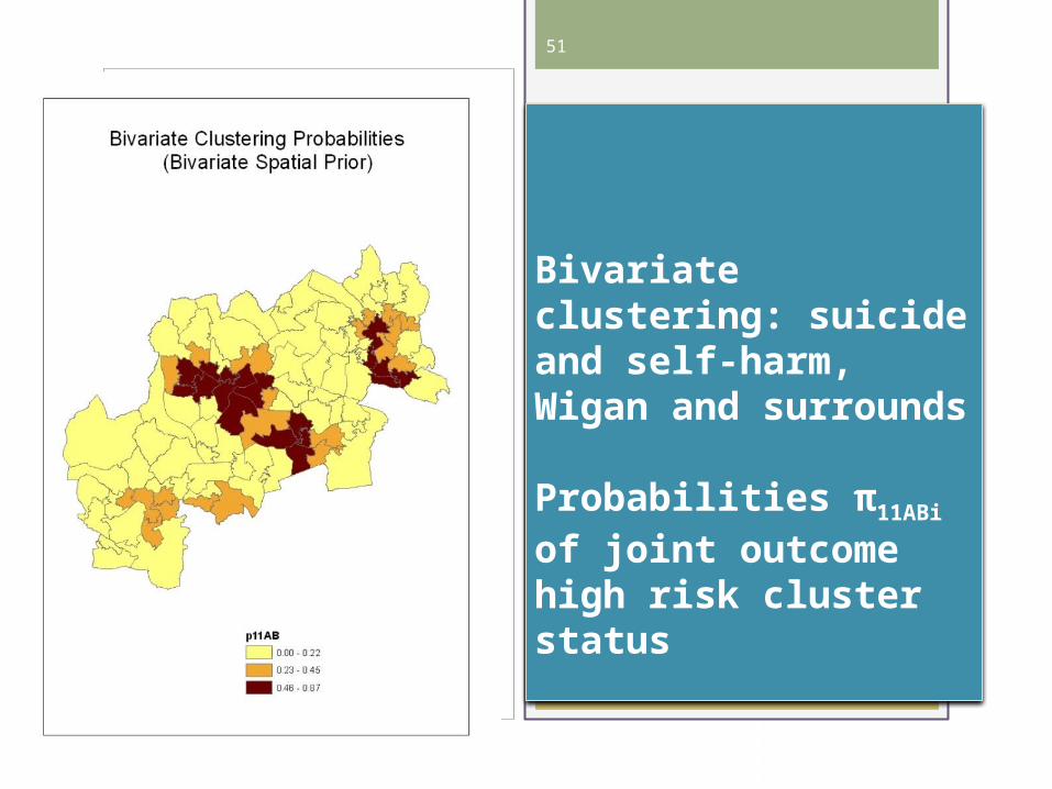
51

Bivariate clustering: suicide and self-harm, Wigan and surrounds

Probabilities π11ABi of joint outcome high risk cluster status

52

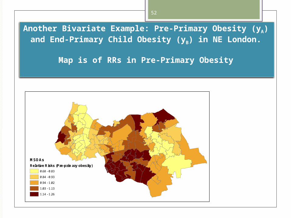
Another Bivariate Example: Pre-Primary Obesity (yA) and End-Primary Child Obesity (yB) in NE London.

Map is of RRs in Pre-Primary Obesity

MSOAs

Relative Risks (Pre-primary obesity)

0.68 - 0.83

0.84 - 0.93

0.94 - 1.02

1.03 - 1.13

1.14 - 1.26

53

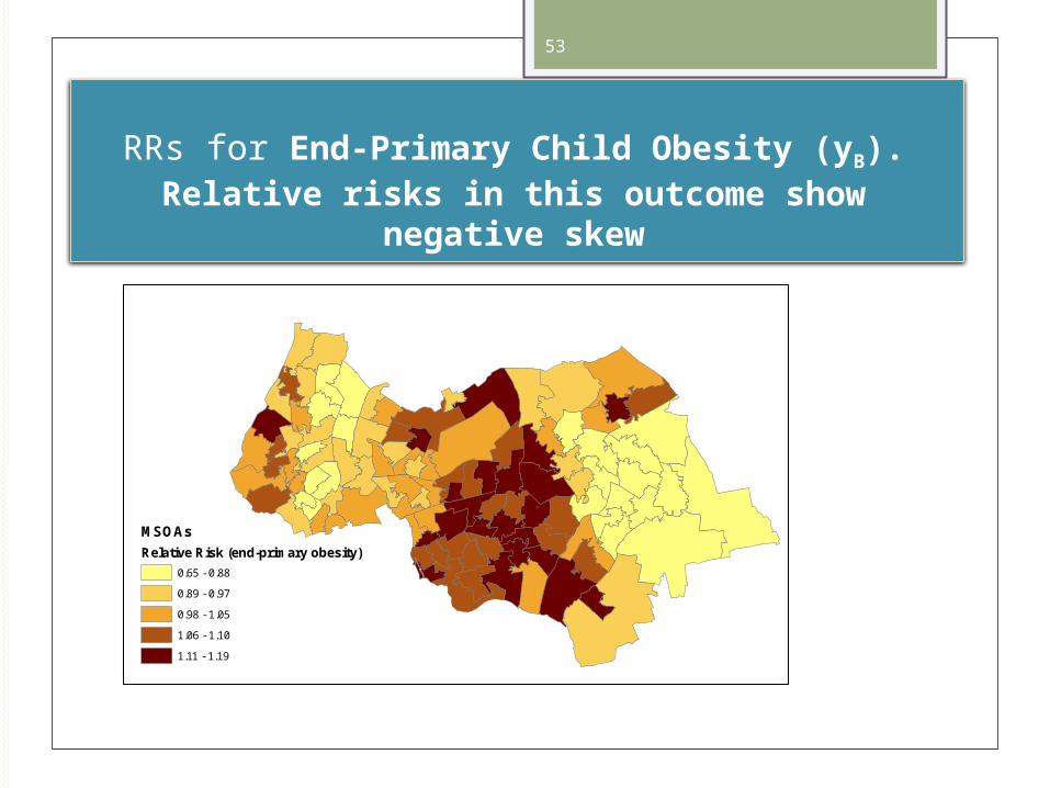
RRs for End-Primary Child Obesity (yB).Relative risks in this outcome show

negative skew

MSOAs

Relative Risk (end-primary obesity)

0.65 - 0.88

0.89 - 0.97

0.98 - 1.05

1.06 - 1.10

1.11 - 1.19

54

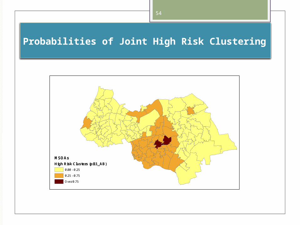
Probabilities of Joint High Risk Clustering

MSOAs

High Risk Clusters (pi11_AB)

0.00 - 0.25

0.25 - 0.75

Over 0.75

55

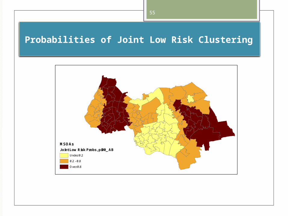
Probabilities of Joint Low Risk Clustering

MSOAs

Joint Low Risk Probs, pi00_ AB

Under 0.2

0.2 - 0.8

Over 0.8

56

Final Thoughts

Cluster status approach provides alternative/complementary perspective to “list of areas” approach, and provides additional insights with regard to cluster centres vs edges, low risk clustering as well as high risk clustering in an

integrated perspective, high/low risk outliers Allows assessment of impacts of covariates on spatial clustering

Can also apply bivariate method when outcome A is disease, outcome B is risk factor. Detects varying strength of association between disease and risk factor