Measuring Reporting Conservatism

Dan Givoly,* Carla Hayn** and Ashok Natarajan***

November 2005 Version

Corresponding Author: Carla Hayn (chayn@agsm.ucla.edu) Key Words: Conservatism, Asymmetric Timeliness, Disclosures, Quality of Earnings, Earnings Management, Accruals.

_________________________________

* Smeal College of Business, Pennsylvania State University, ** The Anderson School Graduate School of Management, University of California – Los Angeles, *** California State University – Pomona We are grateful for the comments made by Helen Adams, Sudipta Basu, Doug Hanna, Jack Hughes, Shiva Rajgopal, Terry Shevlin, D. Shores, Doug Skinner, Charles Wasley, Michael Williams, Joanna Wu, Jerry Zimmerman and participants at the workshops at University of Arizona, University of California-Los Angeles, University of Illinois, University of Rochester, University of Texas at Dallas, University of Washington, Pennsylvania State University and Southern Methodist University.

Measuring Reporting Conservatism

Abstract

The paper examines the power and reliability of the differential timeliness (DT) measure developed by Basu (1997) to gauge reporting conservatism. We identify certain characteristics of the information environment unrelated to conservatism that affect the DT measure and find that it is sensitive to the degree of uniformity in the content of the news during the examined period, the types of events occurring in the period, and firms’ disclosure policies. Our tests, based on both actual and simulated data, indicate that assessing the extent of reporting conservatism requires the recognition of, and control for, these characteristics. We also find that the difference in the timeliness of reporting bad versus good news is likely to be more pronounced than previously reported. Further, we provide additional evidence on the negative association between the DT measure and alternative aspects of conservatism, suggesting that the exclusive reliance on any single measure to assess the overall conservatism of a reporting regime (firms, countries or time periods) is likely to lead to incorrect inferences.

Measuring Reporting Conservatism

1. Introduction

Accountants, regulators and academics have long struggled with the need to operationalize

qualitative properties of financial reporting systems such as objectivity, reliability, consistency,

comparability and materiality. Indeed, some attempts have been made to quantify the attributes of

materiality (Cho, Hagerman, Nabar and Patterson (2003), Pany and Wheeler (1989)), reliability

(Barth and Clinch (1998), Entwistle and Phillips (2003)), and comparability or heterogeneity

(Defond and Hung (2003)).

With some exceptions such as Hagerman and Zmijewski (1979, 1981), Staubus (1985) and

Leftwich (1995), little attempt has been made over the years to quantify conservatism, despite it

being one of the most prominent characteristics of financial accounting. One measure of

conservatism that emanates from the work of Feltham and Ohlson (1995) is the expected market-

to-book ratio. This ratio has been used to gauge changes in reporting conservatism over time (e.g.,

Ahmed, Morton and Schaefer (2000), Beaver and Ryan (2000), Givoly and Hayn (2000), Stober

(1996)) and, coupled with other financial ratios, to measure conservatism across countries (Joos

and Lang (1994)).

Basu (1997) introduced a number of measures that capture the essence of the conservatism

principle as reflected in the adage “anticipate no profits but anticipate all losses.” That is,

conservative reporting means that events with an expected unfavorable outcome are recognized

promptly in income whereas the recognition of the effects of expected favorable events is

deferred. Basu’s most commonly used measure relates to the speed of response of accounting

earnings to bad news relative to good news where the news content is determined by the sign of

the period’s return.. This measure has been used in numerous studies to assess the extent of

accounting conservatism. These include studies dealing with the variation of conservatism across

firms (Basu (1997), Kwon (2002), Huijgen and Lubberink (2003), Chandra, Wasley and Waymire

(2004)), changes in conservatism across time periods (Basu (1997), Givoly and Hayn (2000),

Holthausen and Watts (2001), Raonic, Mcleay and Asimakopoulos (2004), Sivakumar and

Waymire (2003)), its variability over quarters (Basu, Hwang and Jan (2001a)), its relation to the

audit work and auditors’ exposure to legal liability (Basu (1997), Basu, Hwang and Jan (2001b),

Krishnan (2005a and 2005b), Gul, Srinidhi and Shieh (2002), Ruddock, Taylor and Taylor (2004),

Chaney and Philipich (2003), Kelley, Shores and Tong (2004), its impact on the cost of equity

2

(Francis, LaFond, Olsson and Schipper (2004)), its relation to the composition of the board of

directors (Beekes, Pope and Young (2003)), its cross-country variation (Ball, Kothari and Robin

(2000), Ball, Robin and Wu (2003), Bushman and Piotroski (2004), Cao and Lee (2002), Giner

and Rees (2001), Jindrichovska and Kuo (2003), Peek, Buijink and Coppens (2004), Pope and

Walker (1999), Tazawa (2003)), and the trend in the information content of accounting numbers

(Ryan and Zarowin (2003)).1 For a comprehensive analysis of the causes for conservatism and an

extensive review of the related research see Watts (2003a, 2003b).

Given the widespread use of Basu’s measure of differential timeliness to gauge conservatism,

a critical evaluation of the measure is in order. In a recent study, Dietrich, Muller and Riedl (2003)

question the validity of the reverse regression model to measure conservatism, raising a number of

econometric issues. In this paper, we assume that the model is valid and investigate the power and

reliability of the differential timeliness (hereafter DT) measure to gauge the degree of reporting

conservatism of various reporting regimes.2 We first provide evidence suggesting that the DT

measure suffers from serious measurement errors. We then identify characteristics of the firm’s

information environment that affect the DT measure yet are unrelated to reporting conservatism.

The effect of these characteristics on the DT measure is examined using both simulated and actual

data. The evidence suggests that inferences regarding the variation of conservatism across firms,

periods, countries or other reporting regimes cannot be reliably made based on the DT measure

without controlling for certain characteristics of the information and disclosure environments of

the compared samples. Such controls, however, are not easy to implement.

Finally, we discuss the association between the DT measure and other dimensions and

measures of conservatism. We provide additional evidence to that of previous studies showing that

this association is negative, which suggests that the DT measure and, more generally, any single

measure of conservatism, is insufficient to assess all dimensions of conservatism in the sample of

interest. We further propose that within the framework of current U.S. GAAP, other dimensions of

conservatism are more subject to discretion by management and standard setters, rendering them

potentially more insightful than the DT measure in studying the reporting choices and standards

development in different reporting regimes.

1 The underlying logic of the measure, although not the measure itself, has been recently applied to the analysis of the management compensation structure (Leone, Zimmerman and Wu (2004)). 2 As explained in section 7, our analysis and findings are to a large extent independent of those of Dietrich, Muller and Riedl (2003).

3

The paper contributes to the literature on accounting conservatism by providing evidence on

the power and reliability of the widely used differential timeliness measure to gauge conservatism.

Through the identification of factors that bias or otherwise increase the estimation noise of this

measure, the paper points to types of research questions for which the measure is less appropriate

and circumstances where it is likely to yield biased inferences regarding the degree of

conservatism, and suggests situations where alternative or supplementary measures of

conservatism should be employed.

The paper proceeds as follows. In the next section, we provide a brief description of the

differential timeliness measure. Our sample and the data used in the various tests are described in

section 3. Section 4 provides evidence on anomalous behavior of the DT measure that is indicative

of its sensitivity to information characteristics. In section 5 we discuss information characteristics

that are hypothesized to contribute to this measurement error, test for their presence and examine

their influence on the DT measure. Section 6 contains a discussion of the various aspects of

accounting conservatism and their relation to each other. A summary and concluding remarks are

provided in the final section of the paper.

2. The Differential Timeliness (DT) Measure

In conservative reporting, earnings reflect bad news more quickly than they do good news.

Identifying the nature of the events affecting a company by the sign of the stock returns over a

given time period with positive (negative) returns signifying “good” (“bad”) news, Basu’s (1997)

primary measure of conservatism is based on the extent to which the earnings-return association is

stronger during periods of bad news as compared with periods of good news. This differential

timeliness measure is the coefficient β2 in the regression:

EPSjt/Pricejt-1= α0 + β0*DUMjt + β1*Returnjt + β2*(DUMjt*Returnjt) + εt (1)

where the j and t subscripts denote the firm and period, respectively. EPS is the earnings per share

from continuing operations and Return is the firm’s return computed, alternatively, over the fiscal

year or the 12-month period beginning nine months prior to the end of the fiscal year.3 DUM is a

dummy variable that receives the value of 1 if the Return variable for the period is negative and 0

otherwise.4

4 Unless otherwise indicated, we present results based on raw returns and earnings per share from continuing operations. The main restuls of our paper hold when market-adjusted returns are used instead of raw returns and when net income is used instead of income from continuing operations.

4

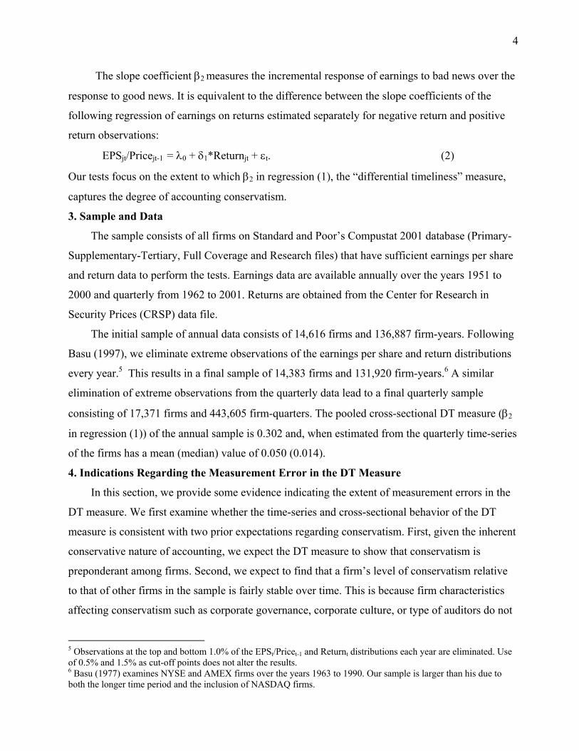
The slope coefficient β2 measures the incremental response of earnings to bad news over the

response to good news. It is equivalent to the difference between the slope coefficients of the

following regression of earnings on returns estimated separately for negative return and positive

return observations:

EPSjt/Pricejt-1 = λ0 + δ1*Returnjt + εt. (2)

Our tests focus on the extent to which β2 in regression (1), the “differential timeliness” measure,

captures the degree of accounting conservatism.

3. Sample and Data

The sample consists of all firms on Standard and Poor’s Compustat 2001 database (Primary-

Supplementary-Tertiary, Full Coverage and Research files) that have sufficient earnings per share

and return data to perform the tests. Earnings data are available annually over the years 1951 to

2000 and quarterly from 1962 to 2001. Returns are obtained from the Center for Research in

Security Prices (CRSP) data file.

The initial sample of annual data consists of 14,616 firms and 136,887 firm-years. Following

Basu (1997), we eliminate extreme observations of the earnings per share and return distributions

every year.5 This results in a final sample of 14,383 firms and 131,920 firm-years.6 A similar

elimination of extreme observations from the quarterly data lead to a final quarterly sample

consisting of 17,371 firms and 443,605 firm-quarters. The pooled cross-sectional DT measure (β2

in regression (1)) of the annual sample is 0.302 and, when estimated from the quarterly time-series

of the firms has a mean (median) value of 0.050 (0.014).

4. Indications Regarding the Measurement Error in the DT Measure

In this section, we provide some evidence indicating the extent of measurement errors in the

DT measure. We first examine whether the time-series and cross-sectional behavior of the DT

measure is consistent with two prior expectations regarding conservatism. First, given the inherent

conservative nature of accounting, we expect the DT measure to show that conservatism is

preponderant among firms. Second, we expect to find that a firm’s level of conservatism relative

to that of other firms in the sample is fairly stable over time. This is because firm characteristics

affecting conservatism such as corporate governance, corporate culture, or type of auditors do not

5 Observations at the top and bottom 1.0% of the EPSt/Pricet-1 and Returnt distributions each year are eliminated. Use of 0.5% and 1.5% as cut-off points does not alter the results. 6 Basu (1977) examines NYSE and AMEX firms over the years 1963 to 1990. Our sample is larger than his due to both the longer time period and the inclusion of NASDAQ firms.

5

fluctuate much over a short period of time. Further, time-varying factors, such as the legal or

regulatory environment, tend to affect the extent of reporting conservatism of all firms operating

in this environment.

4.1. Prevalence of conservatism

Conventional accounting is inherently conservative as evidenced by the fact that net assets

are consistently understated (see Watts (2003a, 2003b)). Aggressive accounting choices by

management may reduce the degree of reporting conservatism but they cannot turn the whole

tenor of the financial statements to being non-conservative or even neutral. In particular, economic

gains will seldom be recognized in earnings earlier than economic losses since GAAP does not

allow recognizing gains before they are realized but permits (and often requires) the recognition of

losses prior to their materialization. Therefore, when the DT measure is used to identify

conservatism, it should detect a clear preponderance of conservative reporting among firms.

To test this prediction, we estimate regression (1) over the annual time-series of firms for

which at least 10 years of data are available from 1951 to 2001 and over quarterly time-series for

firms for which at least 20 quarterly observations are available from 1972 to 2001. To ensure a

sufficient number of “bad news” observations, only firms with at least six observations of negative

returns in the time series are analyzed. The resulting sample consists of 3,181 firm observations

using annual data and 8,687 firm observations using quarterly data.

The results, presented in table 1, show that over 40% of the firms estimated from both the

annual and quarterly data exhibit a negative DT measure. This ostensibly suggests that contrary to

conservative reporting, these firms recognize favorable events in earnings on a timelier basis than

they recognize unfavorable ones. Further, for those firms whose annual (quarterly) data result in a

positive DT measure, the measure is significant for only 15.1% (22.8%) of the annual (quarterly)

cases even at a significance level of only 10%. For the entire annual and quarterly samples, a

significant level of conservatism, as indicated by a positive DT measure at the “lenient” 10%

significance level, is detected only in 7.8% ((15.1% x1,706)/3,181) and 13.5% ((22.8% x

5,143)/8,687) of the firms, respectively.

The failure to detect a significant positive DT measure in the time-series of many firms may

be due to the small number of observations with negative returns and, hence, a low test power. To

increase the power of the test we replicate the tests in table 1 for firms whose quarterly time-series

contains at least 20 (rather than only six) quarters of negative returns and at least 20 quarters of

6

positive returns. This reduces the number of firms to 594 but leaves intact the finding that only a

small percentage of the firms (in this case 18.9%) have a positive and significant DT measure.

The inability of the DT measure to detect the basic conservative posture of conventional

accounting in all, or even a large majority of, firms indicates that the measure is subject to

considerable measurement error or to a downward bias. To gain some perspective on the extent of

this error, we estimate a related time-series parameter, the earnings response coefficient (ERC), δ1

in equation (2), using firms’ annual and quarterly data. This parameter, which captures the

informativeness of earnings numbers, is expected to be positive. Because of measurement errors,

estimates for some firms may not be positive. However, the frequency of an unexpected sign for

the ERC is relatively low. For the annual (quarterly) sample, 9.7% (20.6%) of the firms have a

negative ERC. Of these, only 9.6% for the annual sample and 11.3% for the quarterly sample are

significant at the 10% significance level which translates into only 1%-2% of all firms having

statistically negative ERCs.7 This low frequency of negative ERC coefficients stands in sharp

contrast to the preponderance of firms with a negative DT measure.

4.2. Stability and persistence of conservatism

The firm’s degree of reporting conservatism is affected by certain firm attributes (see Watts

and Zimmerman (1986)). Most of these, such as the corporate culture, firm size, management

incentives or corporate governance, are likely to be fairly stable and would not drastically

fluctuate from one reporting period to the next. This assumption of a relatively stable conservatism

stance is made implicitly by studies on the effect of conservatism on the firm’s cost of capital

(Francis, et al. (2004)), on cross-country differences in conservatism arising from differences in

the legal/judicial system, securities laws, political economy and tax regimes (see, for example,

Ball, Robin and Wu (2003) and Bushman and Piotroski (2004)), and on the differences between

the extent of conservatism in different industries (Kown (2000)) or firms (Krishnan (2005b)). If

the DT measure captures the degree of a firm’s reporting conservatism, it should thus be relatively

stable over time. That is, while firms may gradually, over several years, become more or less

conservative, the extent of their conservatism should not vary significantly from year to year or

from one quarter to the next.

7 The low frequency of negative ERCs is also observed when we limit the number of observations in each time-series estimation to the number of observations that were available to estimate the DT measure (i.e., the number of negative return observations in the time-series).

7

To test the stability of the DT measure over time, we examine the correlation between the

values of firms’ DT measures estimated from successive non-overlapping periods. For this

analysis, a sample of firms with at least 80 quarters of uninterrupted data over the period from

1981 to 2000 is drawn. The 80-quarter time-series of each firm is then divided into successive,

non-overlapping subperiods each consisting of, alternately, 40 quarters (for a total of two 10-year

subperiods), 20 quarters (four 5-year subperiods) and 10 quarters (eight 2½-year subperiods).

Regression (1) is estimated from the quarterly time-series of the firm in each subperiod to derive

β2, the DT measure. We then compute the correlation coefficient across the sample firms between

their DT measures in any two successive subperiods. To control for the possibility that the

earnings response to both good news and bad news moves up or down in tandem over time, we

repeat the above analysis using, instead of the DT measure, a differential timeliness ratio. This DT

ratio, introduced by Pope and Walker (1999), is measured as (β1 + β2)/ β1 using the coefficients

from regression (1).

The results of this stability test, reported in table 2 (columns two and three), indicate that the

DT measure is not stable over time. The association between the DT measure in successive

subperiods of 10 years, 5 years or 2½ years is non-existent, with virtually all of the correlation

coefficients (both Pearson and Spearman rank order) being insignificantly different from zero.

Similar results (not tabulated) are obtained for the DT ratio. These results are in apparent conflict

with the notion that the degree of reporting conservatism is a fairly stable firm characteristic.

To put the stationarity of the DT measure in perspective, we compare it to that of three other

measures of conservatism used by researchers, the book-to-market ratio (Stober (1995)),

cumulative discretionary accruals8 (Givoly and Hayn (2000), Ahmed, Billings, Morton and Harris

(2002)) and the persistence of losses versus profits9 (Basu (1997), Ball and Shivakumar (2005)),

as well as to two other estimates of fundamental attributes of the firm – its earnings response

coefficient (ERC) and its beta. Similar to conservatism, these attributes represent characteristics of

the firm’s operating and economic environment that are expected to be fairly stable over time.

8 Cumulative discretionary accruals are measured as the accumulation over time of [total accruals – operating accruals – depreciation and amortization] standardized by total assets at the beginning of the accumulation period., Operating accruals equal the [change in accounts receivable + change in inventories + change in prepaid expenses - change in accounts payable - change in taxes payable] (see Givoly and Hayn (2000)). 9 The differential persistence of good versus bad earnings news is measured by α3 in the following equation: ∆NIt = α0 + α1D∆NIt-1 + α2∆NIt-1 + α3D∆NIt-1*∆NIt-1 + µt, where ∆NIt is change in income (alternatively defined as including and excluding extraordinary and exceptional items) from fiscal year t-1 to t, scaled by beginning book value of total assets. D∆NIt-1 is a dummy variable taking the value 1 if ∆NIt-1 is negative and 0 otherwise (see Basu (1997)).

8

Like the DT measure, these measures are also subject to measurement error which tends to

dampen their measured stability over time. Nonetheless, the results reported in Table 2 show that,

in sharp contrast to the DT measure, the other five measures are fairly stable over time. This

finding suggests that the intertemporal instability in the DT measure is unlikely to be due to shifts

in the firm’s fundamental characteristics.

Because many studies estimate the DT measure from annual data, we also compute the

correlation between the estimates of this measure made from annual data over two successive

periods of 20 years each (spanning the years 1962 to 2001). The results (not tabulated) based on

the 146 firms that existed throughout this period indicate that the correlation coefficient between

the measure in the two 20-year periods is low, 0.06, and insignificant. Again as a benchmark, the

respective correlation coefficients between the values of the mean book-to-market ratios, the

ERCs and the firms’ betas in the two 20-year periods are much higher and significant at 0.654,

0.189 and 0.756, respectively.

Arguably, the level of a firm’s conservatism could change over a long period such as 20

years. Even the shortest period over which we assess the stability of the DT measure, 2½ years,

may be too long for the purpose of this analysis, leading to the low correlations reported in Table 2

for the DT measure. To gain insight on the extent of the stability of the DT measure over very

short periods, we conduct the following analysis. For each firm with at least 20 quarters of data,

we randomly select one half of the quarterly observations over the available time interval, estimate

the DT measure based on these observations and rank firms by that measure. We repeat this

process for each firm, using the remainder of its quarterly observations and compute a rank

correlation coefficient between the two rankings. A strong correspondence between the firm’s

rankings obtained from the two different subsets of its quarterly data is consistent with the notion

that conservatism is a fairly persistent trait that does not fluctuate from quarter to quarter.

To partition firms into two subsets, we first order a firm’s quarters in a chronological

sequence and. then assign them to one of the two subsets based on the following algorithm. If the

year to which the quarter belongs is odd and the quarter is even, or vice versa, the quarterly

observation is assigned to the first subset. If both the year and the quarter are either odd or even,

the quarterly observation is assigned to the second subset. This procedure assures that adjacent

quarters in the same year always belong to different subsets and that the fiscal quarters are evenly

9

distributed across the two subsets thus preventing any effects of seasonality from clustering in a

subset.10

The results of this “persistence” test are reported in table 3. Even within alternating quarters

of the firm, the DT measure appears to oscillate significantly. Of the firms that are identified by

this measure as being among the 10% most conservative reporters based on a random half of their

quarterly observations (subset 1, portfolio 1 in the table), 37% (those found in portfolios 6 to 10

for subset 2, 2.02% + 5.14% + 4.98% + 8.72% +16.51%) are classified by the measure as being

among the 50% most aggressive reporters when the DT measure is estimated from the other half

of the firms’ quarterly observations. Similarly, of the firms identified by the measure as the 10%

most aggressive reporters based on a random half of the firms’ time-series observations (subset 1,

portfolio 10), 54% are classified by the measure as among the 50% most conservative reporters

when the DT measure is estimated based on the other half of the firms’ quarterly observations.

Thus, for a significant portion of the sample, depending on which quarters of the firm’s time series

are randomly included in the analysis, the firm may appear to be among the more conservative, or

the least conservative, reporters. There is however some tendency of firms assigned to the extreme

portfolios (portfolios 1 and 10) based on their DT measure in one subperiod to remain in those

portfolios when the DT measure is estimated from an alternate subperiod.

Summarizing the above results by a single measure, we find that the rank correlation between

the two portfolio ranks (1 to 10) of the 6,429 firms, each based on a different half of the firm’s

time series observations, is low, 0.063, as is the correlation across these firms between their two

individual conservative rankings (1 to 6,429), of 0.061.11,12 Repeating the analysis using the DT

ratio, ((β1 + β2)/β1, and a subsample of 5,532 firms that have at least 15 quarters with a positive

return and 15 quarters with a negative return (in order to increase the power of the test) produces

essentially the same results.

10 We use two other procedures to partition each firm’s time-series into two subsets, with essentially the same results. In the first of these, the quarters were ordered chronologically and then assigned, alternately, to one of the two subsets. This approach assures that each subset represents all subperiods of the firm’s time series. In the other procedure, we randomly assigned quarters to one of the two sets, with even probabilities. 11 We performed a similar examination for annual data, separating each firm’s data into two subsets of odd and even years and computing the DT measure over both of the subsets. The correlations between the two measures as well as between the portfolios ranks (which were about 0.03) were even lower than those reported for the quarterly data. 12 The results concerning the instability of the DT measure are potentially related to the finding that only a relatively small number of firms have a significantly positive time-series DT measure. This is because instability reduces the likelihood of finding significant values of the measure. Note, however, that, the degree of the measure’s stability over time affects the significance of both positive and negative values of the measure.

10

To provide a benchmark for this last finding, we examine also the correlation across firms

between their two subperiod rankings of the book-to-market ratio, the ERC and beta. In contrast to

the low rank order correlation of 0.061 for the firms’ DT rankings in the two random subsets of

the time-series, the respective correlations for the book-to-market ratio, the ERC and beta (not

tabulated) are 0.949, 0.134 and 0.260, respectively.

The lower stability of the DT measure relative to other economic parameters of the firm

might be due to the fact that unlike the other parameters examined, the DT measure is estimated

over fewer observations (i.e., the subset of periods with negative returns). To rule out this

explanation for the findings we “level the playing field” and replicate table 3 by estimating the

book-to-market ratio, the ERC and beta in each of the two randomly-drawn subperiods (that are

used to derive the correlation coefficients between subperiods) using the same number of

observations used to estimate the DT measure. The results (not tabulated) continue to show that

the other variables are still far more stable. The Spearman rank correlation coefficients between

the two values of the variable estimated from the two randomly-drawn subsets of the firm’s time-

series are 0.725 for the book-to-market ratio, 0.131 for the ERC and 0.386 for the beta, with all

three coefficients being statistically significant at the 1% level or higher.13

4.2.1. Stability of cross sectional estimates of the DT measure

The results above concerning the stability of the DT measure rely on time-series estimates

of that measure. However, many studies estimate the DT measure cross-sectionally, within a given

sample, an industry or a country. In this section we extend the analysis to the stability of

inferences based on cross-sectional estimates of the measure.

In our first examination of whether a given cross-sectional estimate of the DT measure

remains stable over time, we begin by dividing firms into ten equal-sized portfolios based on the

magnitude of their time-series DT measure calculated over the prior 40+ quarters of available data

ending with quarter 4 of 1988. Portfolio 1 contains firms that are the least conservative (i.e., have

the lowest DT measure) and portfolio 10 contains firms that are the most conservative (i.e., have 13 The instability over time of the DT measure could be explained by the fact that investors adjust their firm valuation based of the perceived level of reporting conservatism and that such perceptions may fluctuate over time. Note however that market perceptions of the degree of conservatism inherent in the reported numbers are manifested in the market response to earnings disclosures during the short interval of the earnings announcement period. In contrast, the DT measure relies on long windows to measure the earnings-return association. Nonetheless, we assess the potential effect of the variability over time in the market response to earnings releases on the estimated DT measure by replicating the results of tables 2 and 3 using the return over the period excluding the earnings announcement interval (defined as days -1 to +2 relative to the earnings announcement date). The results concerning the stability of the DT measure are essentially unchanged.

11

the highest DT measure). We next compute the cross-sectional DT measure of firms in the ten

portfolios over each of the nine quarters beginning with the last quarter of the time-series (quarter

4, 1988), Q0, and going forward eight quarters to Q8 (quarter 4, 1990). We rank the portfolios in

each quarter, Q0–Q8, based on the magnitude of their cross-sectional DT that quarter. To assess the

stability of the cross-sectional DT measure, we examine the correlation between the portfolios’

quarterly DT rankings. We repeat this analysis 44 times, moving one quarter forward each time.14

The number of distinct firms participating in each iteration varies somewhat depending on the

number of firms with sufficient data, ranging from 1,360 to 2,440. This results in cross-sectional

estimates within each portfolio from 136 to 244 firm-quarter observations.

The results of the 45 cross-sectional analyses are aligned across the quarters, Q0-Q8 and

presented in table 4. The average DT measure of each portfolio derived from the firms’ time series

is presented in column two. By design, it ranges from the lowest value in portfolio 1 (of -0.147) to

the highest value in portfolio 10 (of 0.301). The results in column three show that in Q0 (the last

quarter of the time-series estimation), the pattern of the cross-sectional estimates of the DT

measure over the 10 portfolios corresponds closely to the pattern of the DT estimated from the

firms’ individual time-series. That is, when pooled cross-sectionally, observations belonging to

firms that exhibit the highest (lowest) time-series values of the DT measure also have the highest

(lowest) cross-sectional DT measure. This pattern is partially maintained in the following quarter,

Q1. However, after two or three quarters, the pattern in the cross-sectional DT measure across

portfolios completely dissipates. In fact, from Q5 onward, the cross-sectional DT measure of

portfolio 10 (the portfolio of firm-years belonging to firms with the highest time-series DT

measure as of Q0) is even lower than the DT measure of portfolio 1. Further, the DT values for

portfolios 1 and 10 over the eight quarters subsequent to Q0 do not differ much from each other on

average as seen by the results in the last column of table 4.

To further assess the cross-sectional stability, we revisit the analysis of Ball, Kothari and

Robin (BKR) (2000) who investigate the relative conservatism of common law countries

(Australia, Canada and the U.S.) and code law countries (France, Germany and Japan) over the

1985-1995 time period.15 Their results, based on samples pooled across countries and years, show

14 The second analysis thus begins with forming 10 portfolios based on the firms’ DT measures estimated for the 41+ quarters of data ending with quarter 1 of 1989, and then estimating the DT measure cross-sectionally for each of these portfolios beginning with quarter 1 of 1989 (Q0) and going forward eight quarter to quarter 1 of 1991 (Q8). 15 BKR narrowed the country groups to these countries to assure that each country is represented in the analysis by at least 1,000 firm-years.

12

that the DT measure of common law countries is significantly higher than that of code law

countries (0.31 vs. 0.01, see their Table 3, Panel A). This, as well as other results, led BKR to

conclude that code law countries report less conservatively than do common law countries.

We begin by replicating their test for a different, slightly overlapping, period consisting of

the ten years from 1994-2003.16 Estimating the DT measures for each of the two groups, pooled

over countries and years produced results qualitatively similar to those obtained by BKR. We find

DT measures of 0.27 and. 0.13 for common law and code law countries, respectively, as reported

in table 5, panel A. We then conduct the same analysis for individual years. If the hypothesis that

common law countries are more conservative holds, we would expect that in any given period, any

common law country would show a higher DT measure than any code law country.

To test this expectation, we ranked the DT measures obtained for each of the six countries

in the two groups. The results, presented in panel B of table 5, show that the ranking of the six

countries is inconsistent over time. Only in one of the ten years (2001) did all three common law

countries have a higher DT measure than all three code law countries. Australia, a common law

country, had one of the highest three DT measures in only four of the ten years, while Germany, a

code law country, enjoyed a top-three DT measure in five out of the ten years. In fact, a code law

country had the highest DT measure (e.g. a rank of 1) in five of the ten years.

These annual results do not consistently support BKR’s main hypothesis that the accounting

in common law countries is more conservative than that in code law countries. The difference

between the pooled results and the individual years’ results is due to the instability of the cross-

sectional DT measure over time even within a given reporting regime.17 These results as well as

those reported in tables 2 and 3, are puzzling since one would expect that the degree of

conservatism exhibited by a firm to be a relatively long-term characteristic of the firm’s reporting

system, spanning several years. A firm’s level of conservatism is definitely not expected to be

16 Global Vantage no longer makes data available prior to 1994. 17 Yearly comparisons between countries represent a stronger test of the hypothesis concerning the relative conservatism of common law versus code law countries than a comparison of pooled observations. If the hypothesis holds, common law countries should exhibit a greater degree of conservatism each and every period. Even if one believes that a pooled sample across countries and years is the proper methodology for testing the hypothesis, the dominance of U.S. and Japanese observations in the pooled samples of their respective groups (in which they represent 81.3% and 78.2% of the firm-years, respectively) raises some concerns about the generalization of the results. In fact, replicating the analysis over the years 1994-2003 on observations from all 23 countries classified by BKR excluding the U.S. and Japan, produces results that are inconsistent with the hypothesis of differential conservatism across the two groups of countries. Specifically, the DT measure of the common law countries excluding the U.S. is 0.08 which is lower, but not significantly different, from that of the code law countries excluding Japan of 0.11.

13

only a one-quarter phenomenon, as suggested by some of our results. In the following section we

continue to test the validity of the DT measure by examining whether it provides results consistent

with a number of additional prior expectations about what the measure should capture.

4.3 Ability of the DT measure to detect “situational” non-conservative reporting

If the DT measure correctly portrays the reporting stance of firms, we would expect that it

would be lower for periods where earnings are known to have been managed upward through the

accelerated recognition of revenues or gains or the deferred recognition of costs or losses. To

examine whether the DT measure indeed detects such “situational aggressive reporting,” we

examine two groups of firms where earnings are likely to be managed upward. Past research

suggests that during periods preceding stock or debt issuances, firms seek to improve their

reported performance by managing earnings (see, for example, Rangan (1995), Shivakumar (2000)

and Teoh, Welch and Wong (1998)). Another period in which aggressive reporting is likely to

have occurred is one for which earnings are subsequently restated downward. If these situations

are indeed associated with aggressive reporting as suggested by anecdotal evidence and by

previous research (e.g., Livnat and Tan (2004)), one would expect that the DT measure detects

them as such.

We identify “big issuers” as firms making the most sizeable capital issuances each year,

defined as those in the top 10% of the distribution of the rate of change that year in the growth rate

of total equity and long-term debt. As a benchmark against which to judge their DT measure, we

examine two control groups, one consisting of all other firms in that year and another composed of

firms within the same four-digit SIC industry group that are the closest in size and profitability in

that year to the big issuer. We estimate regression (1) over the two years immediately preceding

the issuance year (the year for which the rate of change in long term capital is measured).

To form a sample of “restaters,” we identified 162 firms in the U.S. Government Accounting

Office restatement database that announced in 2000 or 2001 that they were restating downward

previous financial statements due to revenue recognition or cost/expense problems. All of these

firms restated their earnings for at least two previous quarters, with most of them restating the

results for reporting periods going back up to three years. We estimate the DT measure from a

pooled, cross-section of their data over the three years preceding the restatement announcement

year, some or all of which reflect overstated earnings and thus aggressive accounting. As a

benchmark, we contrast the estimated DT coefficient with those estimated for the rest of the firms

14

that did not restate their earnings over the same time period and for a group of firms operating in

the same industries as the restaters.

The results are reported in Table 6. The two groups suspected of aggressive accounting show

indeed a significantly greater accumulation of non-operating accruals than their respective control

samples (see the third column of the table), 18 an indication of an upward earnings management

(see Givoly and Hayn (2000)). Yet the DT measure of 0.216 for the big issuers indicates that these

firms are reporting as conservatively (if not slightly more so) as are the firms in the two control

groups (with DT measures of 0.191 and 0.196, respectively).

Similar to big issuers, restaters show a greater accumulation of positive accruals than their

respective control groups, consistent with aggressive accounting. Restaters are expected to have a

lower DT measure over the years where earnings were eventually restated downward. Yet the

estimated DT measure for the restaters sample is 0.116, higher than the DT measure for the other

firms that did not restate their earnings over this time period and significantly higher (at the 5%

level) than the DT measure for firms operating in the same industries during the restated periods of

0.077. Rather than reflecting the aggressiveness of the restaters, the DT measure appears to

indicate that these firms were more conservative than the control groups in the very periods where

earnings were overstated.

The instability of the DT measure discussed in the prior section and its failure to detect

conservatism in situations when it is likely to exist and, contrarily, its detection of conservatism

when it is not likely to be present is perplexing given the intuitive appeal of the measure and its

theoretical underpinnings. In the following section, we identify factors that lead to fluctuations in

the measure that are unrelated to conservatism and that may explain why conservatism is not

reliably reflected in the DT measure as documented in the results thus far.

5. Sensitivity of the DT Measure to Factors Unrelated to Conservatism

In this section we identify a number of factors that are not related to reporting conservatism

but that, nonetheless, are likely to affect the DT measure. The first factor arises from the fact that

the differential timeliness attribute of conservatism is defined with respect to individual economic

events, or shocks, and their earnings consequences while the variables used to estimate the DT

measure are an aggregation of the events (proxied by the return for the period) and their aggregate

effect on earnings (the earnings for the period). Below we analyze whether the presence of

18 Non-operating accruals are defined in footnote 8.

15

conservatism at the individual event level translates into observed conservatism when tested using

aggregate measures of earnings and returns.

We then identify other factors that, while unrelated to conservatism, may affect the DT

measure. These factors, discussed in sections 5.2 and 5.3, pertain to the nature of the economic

events occurring in the examined period and to the firm’s disclosure policies. By affecting the DT

measure these factors influence inferences based on this measure regarding differences in the

degree of conservatism across reporting regimes.

5.1. Aggregation of events

The notion underlying the DT measure is that conservatism is captured by the differential

incremental effect of individual events on current earnings as a function of the nature of the event

(good or bad). However, the economic events and their economic impact are not observable, nor is

their incremental effect on earnings. Instead, the DT measure is estimated from observations on

aggregate earnings for the period and the cumulative economic impact of the period’s events as

gauged by the sign of the cumulative stock return over the period. The relation between aggregate

earnings and the cumulative return is not necessarily reflective of the relation between the

incremental earnings responses to the economic content of the individual events. Thus, while

accounting may be conservative with respect to individual events, this reporting conservatism may

not be captured by the DT measure which is based on aggregated data. In fact, the simulation

analysis presented in this section demonstrates that the use of a period’s aggregated earnings and

cumulative return to estimate the DT measure obscures the presence of conservatism even when it

is present in the data. Results from tests on actual data, described in the next section, support this

conclusion.

In the simulation analysis, “economic shocks” (i.e., favorable or unfavorable events) and their

associated return and earnings effects are generated in a manner consistent with reporting

conservatism. By construction, individual bad news events are reflected in earnings on a timelier

basis than are individual good news events. Moving from the realm of single events, we next

measure the returns and earnings of multiple-event periods by aggregating over the period both the

returns and earnings generated by multiple economic shocks. We then estimate the DT measure

from the regression of earnings on returns and examine the sensitivity of the results to the number

of events in the period. The simulation procedure is described in Appendix A.

16

Table 7, panel A presents the cross-sectional estimation of regression (1) based on single-

shock and multiple-shock periods. Consistent with the more timely recognition of bad news to

good news built into the simulation, the DT measure estimated on the sample of single-shock

periods is positive and significant, correctly indicating conservatism. However, when estimated

from aggregated observations (i.e., from periods containing 2, 10 and 20 shocks), the DT measure

fails to detect reporting conservatism even though each individual shock is reflected

conservatively in earnings. Interestingly, these results are not sensitive to the number of shocks in

the multiple-shock period. Even aggregating only two shocks per period eliminates any observable

conservatism inherent in the earnings response to shocks.

The intuition underlying these results is reflected in figure 1. The three scatter diagrams

depict the earnings-return association obtained from the simulation for, respectively, single-shock,

two-shock and ten-shock periods. By construction, the sample of single-shock periods exhibits

conservatism. That is, earnings and returns are more strongly associated for cases of negative

returns than for cases of positive returns. In contrast, when the periods consist of two economic

shocks or events and thus the period’s returns and earnings are the sum of these variables’ values

over the two events, the differential earnings-return association between negative return and

positive return cases disappears (see figure 1, diagram B). This occurs because for approximately

half of the two-shock periods, the two shocks are in opposite directions representing both a

favorable and an unfavorable event. Thus their effects on earnings partially offset each other, with

the stronger shock dominating the period’s cumulative earnings and cumulative returns. When the

dominate shock is positive (negative) both the return and the earnings for the period as a whole

tend to be positive (negative). As a result, the period’s earnings and returns are positively

correlated in the two-shock periods, independent of the sign of the period’s return. The same

aggregation effect is present in all multiple-shock periods.

These results suggest that, depending on the strength of the aggregation effect, the DT

measure likely understates the true level of conservatism or may even fail to detect it even when it

exists. The degree to which the DT measure dissipates upon aggregating events is a function of the

relative impact of the individual economic shocks. When the magnitude of one or a few shocks in

the period dominates that of the others, the offsetting effect of aggregation is weaker and the

conservatism that characterizes the reporting accounting treatment of individual shocks is still

retained even under aggregation. This point is demonstrated in panel B of table 7. As the results

17

show, when a certain proportion of the shocks (10% in the example) are “extreme” in the sense

that they have a higher mean and variance than the other shocks, the dissipation rate of the DT

measure decreases. For example, when the “extreme” shocks are distributed normally with a mean

of ±10 and a standard deviation of 2 as opposed to the other shocks (representing 90% of the

shocks) that are distributed normally with a mean of ±1 and a standard deviation of 0.2, the DT

measure is still positive and significant even when estimated from ten-shock periods.

The DT measure is more likely to capture existing conservatism as the relative frequency of

extreme shocks and their extremity or volatility is higher. This is true even when the number of

shocks over which the period’s earnings and returns are aggregated is large. It can be shown that a

differential response of earnings to individual shocks as a function of the content of the shock

(“good” or “bad”) disappears with aggregation when the probability distribution of the economic

shocks is uniform. However, when the distribution contains extreme (“chunkier”) shocks, as is the

case in an exponential probability distribution, the differential response of earnings to individual

shocks is retained even under aggregation.19 This finding suggests that the effect of aggregation

varies across periods depending on the “chunkiness” of the news. Using the DT measure to gauge

conservatism, periods with a smooth flow of a large number of partially or fully offsetting

economic shocks will not appear to be conservative even if conservative reporting is applied to the

translation of the individual shocks into earnings. In contrast, the DT measure will properly

identify the nature of the reporting regime (countries, industries, firms or periods) when the

observations are dominated by a single or a few large uni-directional economic shocks.

5.1.1. Time-series and cross-sectional aggregation

The discussion so far as well as the simulation model and the results from actual data

(presented below) are all couched in terms of aggregating individual events, or economic shocks,

over time. Note that accounting conservatism may not be exercised continuously in response to

individual economic shocks but rather may be applied discretely, with respect to aggregate

developments in the period. Most notably, the application of the lower of cost or market rule

(LCM) to accounts such as receivables or inventories represents an end-of-period response to

aggregate developments during the period (e.g., deterioration in the creditworthiness of customers

19 We thank Michael Williams for providing a proof of this. The proof and the simulations assume that successive shocks are independent. A positive serial correlation in successive shocks enhances the uniformity of the shocks in the period and attenuates the aggregation effect. The effect of the uniformity of the shocks is tested using actual data in section 5.1.2.

18

or a decline in inventory market prices). One might argue therefore that since conservatism is

applied with an eye to the aggregate effect of events, the degree of aggregation of individual

events over time does not pose a problem for the measurement and interpretation of the DT

measure.

However, conservatism is routinely applied continuously to individual economic (price-

moving) events during the period. For example, the receipt of a new order is not recorded

immediately as revenue, expenditures on internally-developed intangibles are expensed as

incurred, a potential gain from filing a lawsuit is not recognized until settlement and the economic

benefits from a successful acquisition must await their realization. Further, even if all of the

events that trigger conservatism were in the form of end-of-period adjustments, a cross-sectional

aggregation effect would still exist and hinder a correct assessment of conservatism by the DT

measure unless the occurrence of these events and their earnings consequences are both perfectly

and positively correlated. To illustrate, assume at the extreme that all recordable transactions are in

the form of end-of-period adjustments to accounts receivable and inventories. If the write-downs

of inventories are traced to economic events (and hence price movements) that are uncorrelated

with the events that precipitate the accounts receivable write-offs, the aggregation problem will

still be present.

5.1.2. Aggregation effects in actual data

To test the above predictions regarding the effect of the chunkiness or homogeneity of the

economic events during the period on the DT measure, we devise a measure of the extent to which

the period is dominated by a single or a few uni-directional price-moving events. This

“dominance” measure, DOM, is determined as follows. Using the quarterly sample, each firm-

quarter is divided into N intervals consisting of I trading days each where I is alternately 1, 5 or

10. N(I) denotes the number of I-day intervals in the period. For example, when there are 60

trading days in a quarter, N(5) equals 12. We then compute the return over each of the N intervals,

determine the sign of that return, and accumulate the interval returns separately over the positive

and negative return intervals. Denoting the interval accumulation with a total positive or a total

negative return as CUM+ and CUM-, respectively, we define the dominance measure, DOM, for

each quarter as the ratio:

DOM(I) = │CUM+ - │CUM-││ / Larger of {│CUM+│or│CUM-│} (3)

19

By construction, DOM(I) lies between 0 and 1. In periods where the flow of information has

a fairly uniform content (i.e., the events do not offset each other), DOM will be close to 1. At the

extreme, where the content of the news in the interim periods as measured by the sign of the return

for that period is perfectly correlated, DOM equals 1. In general, DOM will receive a high value

when one price-moving event is so dominant as to dictate the sign of the period’s return.

For each interval length I (I=1,5,10), we rank the quarters by their DOM(I) and assign them

to three portfolios, from the top third of the observations (those most dominated by same-sign

news) to the bottom third of the observations (those least dominated by same-sign news). We then

estimate the DT measure across all firm-quarters within each of the three portfolios.

The results, reported in table 8, show that the DT measure decreases almost monotonically as

the events for the period become more diffuse, as indicated by a lower value of DOM. For

example, when the returns are cumulated over 10-day intervals as shown in panel A, the DT

measure for the quarters most dominated by same-sign events (a DOM value of 0.843) is 0.246.

This measure is much lower and statistically insignificant when estimated for quarters with the

least dominant same-sign events (the DOM of portfolio 3 is 0.210 and has a DT measure of

0.027). This same pattern is evident when intervals of 5 days and 1 day are considered.

The results reported in table 8 are reinforced when we correlate the annual values of the DT

measure estimated cross-sectionally with the annual values of the DOM measure computed as

described in (3) above using annual rather then quarterly return data. Figure 2 depicts the time-

series of the annual DT measure and the DOM measures based on 5- and 10-day intervals. As the

figure shows, the measures tend to move in tandem. The correlation coefficient between the

annual DT and DOM measures is 0.480 (significant at the 1% level) for the 5-day interval

calculations and 0.381 (significant at the 5% level) for the 10-day interval calculations. Similar

results are obtained for the DT ratio, (β1+ β2)/β1, which reflects the earnings response to bad news

relative to good news. This strong and significant association suggests that comparisons of the DT

measure between time periods (e.g., between periods with different degrees of litigation risk)

should control for this factor.

Note that DOM is likely to be correlated with return variability: Other things being equal, the

presence of a dominant event associated with a large return corresponds to greater return

variability. Indeed, the correlation coefficient between the standard deviation of the return over the

I-day interval is positively correlated with the standard deviation of the return across these

20

intervals, having a value of 0.489, 0.402 and 0.266 for 1-, 5- and 10-day intervals, respectively. To

control for the return variability effect in determining the effect of aggregation on the measured

DT, we divide the observations in each of the DOM portfolios in table 8 into 10 subgroups

ordered by the standard deviation of the return. The estimates for the DT measure (as well as the

other parameters) for each DOM portfolio are obtained by averaging the estimates from each of

the 10 subgroups. The results (not tabulated) show that the mean DT measures are still

significantly higher for the high DOM portfolio than for the low DOM portfolio.20

The association between the “chunkiness” of the news and the DT measure suggests that this

measure understates conservatism for firms where the information environment is characterized by

a smooth and frequent arrival of news relative to firms for which the news is less frequent and

arrives in “chunks.” The information environment of larger firms is more likely to conform to the

former characterization with the news flow being continuous throughout the period. In contrast,

for smaller firms, news is more likely to occur in clusters around a particular news event with the

result that their period returns will reflect a single or a small number of events.

To test this prediction, we group firms into ten size portfolios each year based on their market

value of equity at the beginning of the year and then estimate the mean DOM measure derived

from daily returns for each portfolio. Table 9 confirms the prediction that the DOM values are

inversely related to firm size. The mean DOM value for the largest 10% of the firms is 0.404 and

increases monotonically as firm size decreases, with the smallest 10% of the firms having a mean

DOM of 0.649.21

Column 3 of the table shows the DT measure for each size portfolio estimated from the

pooled firm-years in each portfolio. Note that the DT measure increases as the firm size goes

down. For firms in the smallest size decile (portfolio 10), the DT measure is 0.314 and it declines

monotonically to 0.113 for the largest firms (portfolio 1). This finding, while consistent with other

studies that use the DT measure to gauge conservatism,22 is a bit surprising in light of the fact that

larger firms are expected to report more conservatively due to their greater exposure to public

scrutiny and thus to greater political costs (Watts and Zimmerman (1986)). Further, larger firms

20 A similar analysis was conducted to control for the positive correlation that exists in the data between DOM and the absolute magnitude of the return. The results regarding the effect of DOM on the DT measure remain intact after controlling for this effect. 21 The results reported are based on DOM computed on 5-day intervals. Similar results are obtained when DOM is based on 1-day and 10-day intervals. 22 22 See for example Basu et al. (2001a and 2001b), Giner and Rees (2001) and Ryan and Zarowin (2001).

21

are likely to have a lower degree of information asymmetry with external parties than smaller

firms (Bhushan (1989)) thereby reducing their incentives to use more aggressive accounting

practices (see Richardson (1997)).

We expect that the higher DT values for smaller firms result from the differential aggregation

effect inherent in measuring the DT value for small versus large firms. To control for the effect of

aggregation, we rank the firm-year observations by their DOM and assign observations to one of

ten DOM portfolios. Next we estimate regression (1) within each firm-size portfolio over the firm-

years in that portfolio that belong to the same DOM portfolio. Finally, we average the estimated

values of each coefficient in regression (1) over the ten regressions within each size portfolio to

derive an “iso-DOM” value of the coefficient.

As shown in column 4 of Table 9, after controlling for the dominance of news events in the

period through DOM, the strong inverse association between firm size and conservatism almost

completely dissipates. The difference between the DT measure of the largest 10% of the firms and

the smallest 10% of the firms shrinks from 0.201 (0.314-0.113) to 0.052 (0.061-0.009). These

findings reinforce the notion that the DT measure is sensitive to the properties of the aggregated

data upon which it relies. They also suggest that the lack of control for the differential sensitivity

of firms to this factor, as captured by DOM, may lead to anomalous results regarding

conservatism.

5.2. The effect of the nature of economic events on the DT measure

The DT measure interprets the differential earnings response to favorable and unfavorable

economic events as an indication of the degree of conservatism. However, regardless of the extent

of reporting conservatism practiced by firms, certain economic events will never, or only

marginally, affect current earnings. Examples of events of this type are the receipt by the firm of a

new long-term contract, a change in interest rates that does not affect existing debt, a new

regulation that will affect only future operations and cash flows, an anticipated (but not yet

enacted) change in the future tax rate, obtaining or failing to obtain FDA approval of a new drug, a

successful invention, or the departure of the CEO. Events of this type change the gap between

market and book values. Yet, their predominance, in terms of both the frequency and economic

significance during the test period, will also affect the magnitude of the DT measure because these

events are likely to affect the current period’s returns but not the current period’s earnings. As a

result, the DT measure will be artificially overstated (understated) for time periods or for firms

22

where there is a preponderance of favorable (unfavorable) events of this type, leading to erroneous

inferences about the degree of reporting conservatism for these periods or firms.

To illustrate, the future effects of current shocks such as a decrease (an increase) in interest

rates will be immediately impounded in stock prices. However, the increase (decline) in earnings

in the current period will only partially reflect that effect. The resulting observation, namely that

earnings do not respond or only partially respond to good (bad) news, will lead unduly to the

inference of conservative (aggressive) accounting.

While these events affect the overall difference between the economic, or market-based,

valuation of income and assets and their accounting valuation, the occurrence of these events is

unrelated to the conservative “behavior” by parties involved in financial reporting. Yet, most

studies on conservatism focus on the behavioral, regulatory or standard-setting aspects of

reporting conservatism. They aim at measuring the “discretionary” component of conservatism

over which, presumably, those involved in producing the financial reports have control. To gain

insight into these discretionary aspects, it is thus necessary to control for the nature of the

transactions and events in the test sample.

The potential effects of positive or negative price-moving events that are not captured in

current income, hereafter referred to as type 1 and type 2 events, respectively, are demonstrated

through a simulation analysis of returns and earnings as described in Appendix B. Results of this

simulation are presented in table 10. Each of the estimations is based on 100,000 observations

generated according to the methodology described in the appendix. As expected, as the test sample

is injected with an increasing number of type 1 events, the DT measure increases, suggesting more

conservative reporting. As Panel A of the table shows, the DT measure, which by construction is 0

under neutral reporting, increases from this 0 starting point to 0.007, 0.016 and 0.039 as the

proportion of type 1 observations increases to, respectively, 10%, 20% and 50%. In contrast,

when the proportion of type 2 events increases in the sample, the DT measure of 0 in the neutral-

reporting base sample becomes increasingly negative, creating the appearance of more aggressive

reporting. Similar directional effects on the DT measure are observed when the base sample

assumes conservative reporting. For this sample, too, the reporting regime as gauged by the DT

measure appears more conservative with the influx of type 1 observations and less conservative

and even aggressive with an increase in the proportion of type 2 events. Similar conclusions about

23

the effect of these price-moving events which have no impact on current period earnings on the

inferences regarding the reporting regime are drawn when the DT ratio is considered.

5.2.1. Effect of the nature of economic events in actual data

The simulation results demonstrate how certain economic events affect the DT measure. In

this section we provide evidence that this effect is present in actual data, and that it could unduly

influence the magnitude of the DT measure thus leading to incorrect inferences about the level of

reporting conservatism.

To provide such evidence, we identify four events that are likely to materially affect firms’

stock prices but which are unlikely to affect contemporaneous earnings. We then examine the DT

measure of samples dominated by such events. The events that we examine are announcements of

acquisition bids, new contracts, lawsuit filings and SEC investigations. Past research suggests that

these events are associated with abnormal returns by, respectively, target firms (see Jensen and

Ruback (1983)), firms that are awarded new contracts, firms against which lawsuits are filed, or

firms being investigated by the SEC (see, for example, Beneish (1999)). These abnormal returns,

however, are unlikely to be related to the profitability of the firm in the current period. To the

extent that the price effects of these events are strong enough to determine the sign of the overall

period’s return, samples with a high frequency of events resulting in positive stock returns that are

unlikely to be reflected in current period’s earnings (e.g., acquisition announcements or contract

awards) are expected to appear more conservative when viewed through the “lens” of the DT

measure. Similarly, to the extent that samples contain firms that experience negative returns

without a corresponding decline in contemporaneous earnings (e.g., lawsuit filings, SEC

investigations), their reporting stance is expected to appear more aggressive as assessed by the DT

measure.

The results are reported in table 11. Both target firms (panel A) and firms awarded contracts

(panel B) have much higher DT measures than comparison groups consisting of the remaining

firm-quarters that were not included in the target sample, a matched group of firms operating in

the same industries and close in size to the two samples, or the same firms one year prior to the

acquisition bid or contract award.

Firms that became defendants in class action lawsuits (panel C) or subject to an SEC

investigation (panel D) show exactly the opposite results. Even though the sample sizes are small

24

and, in the case of the SEC investigation the sample yields a very low adjusted R2, the results are

consistent with the hypothesized dampening effect of these events on the DT measure.

Interpreting the higher DT values of the target and contract-award firms (or the lower DT

values of the sued or investigated firms) as an indication of greater (or lower) conservatism is

technically correct. Yet this assessment of the degree of conservatism is devoid of any accounting

implications since the result reflects the nature of the events experienced by these firms rather than

their reporting stance.

5.3. Interaction between Reporting Conservatism and Disclosure Policies

An implicit assumption in the use of returns to surrogate for news in constructing the DT

measure is that prices reflect all publicly-available information correctly and in a timely manner,

that is, market efficiency is of the semi-strong form. However, assuming the semi-strong form of

efficiency and some managerial discretion over the release time of firm-unique information, the

timing of information disclosures becomes endogenous to management’s discretion regarding the

extent of accounting conservatism in its financial report. In this case, management decisions

concerning the public announcement of information would unduly affect the DT measure. For

example, holding the reporting system constant, firms that tend to disclose good news more

promptly will exhibit a longer lag between the release of good news (relative to bad news) and its

subsequent incorporation in earnings, thus showing a higher DT measure or greater

conservatism.23 In contrast, management with a more “conservative” or cautious disclosure policy

may release bad news more promptly. This will be interpreted by the DT measure as aggressive

reporting since it increases the time lag between the bad news disclosure and its impact on returns,

and the subsequent reflection of this news in reported earnings.24

This interaction between management disclosure policy and the DT measure is of concern in

studies on the differential response of earnings to good versus bad news because the same factors

that affect differential reporting timeliness (such as corporate governance or litigation risk) also

influence disclosure policies. Unless management is assumed to have a neutral disclosure policy, a

fairly tenuous assumption, the DT measure will reflect the differential reporting timeliness with

bias. For example, if a highly litigious environment prompts management to preempt bad news by

23 Such a tendency is consistent with the findings regarding the earlier release of “good news” reports and the delay in the release of “bad news” reports (see Chambers and Penman (1984), Givoly and Palmon (1982)) and McNichols (1988)). 24 This prompt release of bad news is consistent with the phenomenon of “earnings warnings” and the evidence in Skinner (1997).

25

disclosing it early (before it is reported or even reportable under GAAP), the DT measure will

underestimate the degree of conservatism.

Furthermore, substitution may exist between the disclosure and reporting policies. To the

extent that a more conservative reporting strategy permits a more aggressive disclosure policy, the

DT measure will accentuate actual differences in the degree of reporting conservatism. Firms that

have an aggressive (conservative) reporting policy that is “compensated” by a more conservative

(aggressive) disclosure policy will show a higher (lower) DT measure than warranted by their

reporting choices.

While we do not test the effect of this interaction between reporting and disclosure policies, it

should be considered in studies where the factors hypothesized to affect differences in the degree

of conservatism, as assessed by the DT measure, potentially overlap with those affecting

disclosure policies.25, 26

The shortcomings of the DT measure identified in this section are consistent with the

“anomalous” findings reported earlier in the paper. In particular, the aggregation effect and the

nature of the events transpiring during the period are likely to vary from period to period and from

sample to sample and to obscure what might otherwise be stable time-series and cross-sectional

patterns in the behavior of the differential timing aspect of conservatism.

6. Association of the DT Measure with Other Dimensions of Accounting Conservatism

Watts (2003a, p. 208) refers to conservatism as an attribute of financial reporting that relates

“to the cumulative financial effects represented in the balance sheet and to income or earnings

cumulated since the firm began operation.” “Conservative” accumulations result in a systematic

understatement of earnings on the income statement, and, accordingly, an understatement of assets

and equity on the balance sheet.

While the asymmetrical treatment of gains and losses is a major contributor to the systematic

undervaluation of the book value of the firm’s equity as compared to its economic value (see Basu

(1997) and Watts (2003a)), there are other factors that lead to such a “conservative” outcome.

25 Gigler and Hemmer (2001) relate conservative reporting to disclosure policies in a model where firms in less conservative reporting regimes are more likely to provide preemptive voluntary disclosures than firms in more conservative regimes. For the less conservative reporters, returns lead earnings and thus their earnings reflect the news on a more timely basis than firms with more conservative accounting. 26 In countries where insider trading laws are non-existent or not enforced, insider trading is another mechanism through which information is impounded in prices. In these countries, the interplay between inside-information-based trading and the eventual incorporation of this information in the financial statements should be considered in interpreting the DT measure.

26

Recently, Ball and Shivakumar (2005) make a distinction between the asymmetric recognition

feature, which they denote as “conditional conservatism” that arises from the speedier recognition

in earnings of economic losses (i.e., it is “conditional” in that it depends on the occurrence of

losses) and other contributors to the undervaluation of assets, which they denote as “unconditional

conservatism.” They argue that it is the “conditional conservatism” that enhances the quality of

earnings and the usefulness of financial statements, particularly when used for contracting

purposes.

The table provided in Appendix C offers a classification of the sources of conservatism

defined as the systematic understatement of assets on the balance sheet. In the first column, three

sources of such understatement are identified: C1, conservatism that is present as a result of

financial accounting’s failure to capture the positive present value of projects and subsequent

increases in the value of assets; C2, the conservatism resulting from the minimization of the firm’s

assets as reported on the balance sheet; and C3, conservatism resulting from the more timely

recognition of losses relative to gains. The features of financial reporting that contribute to the

three sources of conservatism are indicated in the second column. The third and fourth columns of

the table examine the extent of discretion available to standard setters, regulators and management

with respect to each aspect of conservatism.

As this classification suggests, the historical cost convention, the choices of accounting

methods and estimates within this convention, and the asymmetric recognition rules for gains

versus losses discussed above, all combine to yield a conservative (understated) valuation of assets

and equity.27 This classification allows us to trace the links between the different sources of

conservatism and identify the extent of discretion available to preparers of financial statements

and standard setters in determining the level of reporting conservatism.

One domain of financial reporting where management, auditors and standard setters have

considerable discretion within the historical cost framework is the prescription of certain

accounting methods and the choice of methods and estimates. Another domain with lesser

discretion is the timing of gain and loss recognition, the aspect captured by the DT measure.

27 Other, somewhat overlapping, classifications of conservatism exist. For example, conservatism can be classified into “income statement conservatism” or “balance sheet conservatism” (e.g., ARB 2 (AICPA 1939) and Ball, Kothari and Robin (2000)), “economic value-added” (resulting from investment in positive NPV projects) or “accounting value-added” (Easton and Pae (2003)), “ex-ante” conservatism (the undervaluation of recorded assets) or “ex-post” conservatism (the understatement of income due to the deferred recognition of gains relative to losses) (Pope and Walker (2002)).

27

Focusing on the conservatism inherent in the choices in only one domain will not provide an

accurate assessment of the overall degree of conservatism exhibited by the reporting entity when

the choices made in each domain are independent of each other and, in particular, when they are

substitutes.

In fact, there is likely to be a negative association between the differential timeliness of

reporting gains and losses and other manifestation of conservatism. For example, “unconditional

conservatism” in the form of unduly pessimistic estimates of bad debt provisions or the life

expectancy of long-lived assets, or in the form of a particular cost allocation schemes (such as

LIFO), likely leads to less pronounced timeliness differentials between loss and gain recognition.

In contrast, the earnings of firms that engage in aggressive reporting in the form of extensive

capitalization and inadequate provisions for future costs or losses will be more “time-sensitive” to

the recognition of unfavorable economic events and therefore exhibit a greater degree of

“conditional conservatism.”

This discussion suggests that, other things being equal, the greater is the unconditional

conservatism, the less pronounced is the difference in the response of earnings to bad versus good

news.28 The does not necessarily mean, however, that the DT measure is negatively correlated

with the other aspects of conservatism. For example, firms that employ pessimistic estimates in

their financial reporting (thus undervaluing their assets) may also incorporate adverse economic

developments in earnings much faster than they do favorable news. Further, legal and institutional

factors (such as the link between tax reporting and financial reporting found in code-law countries)

may affect the various dimensions of conservatism differently. Thus, the association between the

DT measure and other dimensions of conservatism is an empirical issue.

The lack of association (and, in fact, a negative association) between the DT measure and

other measures of conservatism has recently been noted by Ball, Kothari and Robin (2000), Basu

(2001), Frances et al. (2004), Giner and Rees (2001), Hanna (2003), Pae, Thornton and Welker

(2005), Pope and Walker (2002) and modeled by Beaver and Ryan (2004) and Roychowdhury and

Watts (2005 We provide additional evidence about the inter-correlation among a number of

proxies of conservatism used in previous research. These are the ratio of the book value of

operating assets to their market value, the amount of “unrecorded reserves” examined by Penman

28 This notion is developed by Beaver and Ryan (2004) who model the relationship between these two distinct concepts of conservatism. Their model captures the probabilistic and history dependent nature of conditional conservatism and appears to be supported by the data (see Beaver et al. (2004)).

28

and Zhang (2002), and the two conservatism measures developed by Easton and Pae (2003).

Penman and Zhang (2002) measure the “unrecorded reserves” as the sum of the hypothetical

advertising and R&D assets and the LIFO reserve, deflated by total operating assets. Easton and

Pae (2003)’s first measure of conservatism is that induced by investment in positive present value

projects. Their second measure provides an estimate of the undervaluation of the book value of

assets arising from accounting rules.29 Easton and Pae’s two measures are operationalized as the

sensitivity of the firm’s current return to, respectively, the change in cash investments and the

lagged change in operating assets. 30 Each of the measures attempts to capture only one of the

various aspects of conservatism. However, their association with the DT measure provides

evidence as to whether the reliance on a single measure to assess the full extent of reporting

conservatism is sufficient to draw conclusions about the level of overall conservatism.

Table 12 presents the Pearson and Spearman rank order correlation coefficients across 16

industry groups between the four measures of conservatism. The table shows that the DT measure

is negatively related to the other measures of conservatism. For industries where reporting is

characterized by the DT measure as relatively conservative, each of the alternative measures

classifies their reporting as relatively aggressive.

A number of studies rely on differences in the DT measure to characterize the degree of

conservatism of reporting regimes, such as countries, periods or industries (see, for example, Gul,

Srinidhi and Shieh (2002), Kwon (2002), and Sivakumar and Waymire (2003)) or to proxy for the

overall conservatism level in researching other issues (e.g., the determinants of cost of capital

(Francis et al. (2004)) or CEO retention decisions (Engel, Hayes and Wang (2003)).The negative

correlation between the DT measure and other dimensions and measures of conservatism suggests

that relying on any single measure is likely to lead to the wrong characterization of the overall

conservatism level.31 However, because the DT measure is the most commonly used measure, the

negative correlation that it exhibits with other dimensions of conservatism is of particular

importance. Another conclusion that can be drawn from the negative correlation between the DT

29 This measure is close in spirit to Penman and Zhang’s “unrecorded reserves” measure and to the type of accounting conservatism stemming from the choice of accounting methods (see Hagerman and Zmijewski (1981)). 30 The change in cash investment is derived from the Statement of Cash Flows as capital expenditures net of proceeds from sale of property, plant and equipment, plus acquisitions minus other investing activities. 31 Some of these concerns are echoed by recent studies (see Beaver and Ryan (2004), Giner and Rees (2001), Hanna (2003), Pope and Walker (2002), and Watts (2003b)).

29

and other conservatism measures is that the DT measure captures a unique aspect of conservatism

not gauged by other measures.

7. Summary and Concluding Remarks

Basu (1997) helped stimulate considerable research on accounting conservatism and his

proposed differential timeliness measure makes a significant contribution to the research on

financial reporting and its economic consequences. The main message from our paper is that the

use of the measure in different research settings should be more selective and qualified.

We demonstrate that the use of the measure leads to anomalous results. In particular, the

measure fails to detect conservatism in instances where it is likely to exist and suggests a high

degree of volatility in the measured degree of conservatism over periods as short as a quarter when

a much more stable pattern is expected.

We identify a number of features of the DT measures that contribute to these results. First,

the measure uses aggregated measures of earnings and returns. This “aggregation effect” unduly

influences the magnitude of the DT measure. It is also affected by the nature of the events

occurring during the period and by firms’ disclosure policies.

When conservatism is defined as the undervaluation of assets relative to their economic

value, it has other sources or dimensions beyond the differential timeliness of gain and loss

recognition. We add to the evidence on the inverse relation between the DT measure and other

dimensions of conservatism, concluding that the measure should be used in conjunction with other

conservatism measures in drawing inferences about the extent of reporting conservatism present in

an examined sample.

The implications of the limitations of the DT measure identified in this study differ across

research settings. To illustrate, for a study like Basu, Hwang and Jan (2001a) which compares the

level of conservatism between the fourth quarter and earlier quarters, the interaction of the DT

measure with other facets of conservatism may not be particularly serious. The relatively short

measurement period, quarters rather than years, reduces the effect of aggregation. Further, because

the comparisons are made between different quarters of the same firm, it is likely that the nature of

the events and the firm’s disclosure policies are similar across quarters, reducing the concern that

these factors will affect the DT measure. In a similar vein, studies that focus on assessing the DT

measure for a single industry (e.g., railroads by Sivakumar and Waymire (2003)) or the

technology sector (e.g., Chandra, Wasley and Waymire (2004)) where the information

30

environment is likely to be similar over time are less likely to be affected by the concerns

regarding the sensitivity of the DT measure to the information environment.

In contrast, studies that compare the degree of conservatism between countries are more

susceptible to the concerns raised here. The substitution effect between the different aspects of

conservatism means that the DT measure captures only a portion of the overall conservatism in the

countries examined. Countries differ widely in the degree of development of their capital markets

and hence in the nature of the information flow. Less developed markets are likely to be

characterized by “chunkier” news arrivals. Further, the different legal and regulatory environments

of different countries are bound to affect management disclosure policies and therefore the DT

measure.

In some settings, the DT measure can be used reliably to gauge conservatism as long as key

assumptions hold (e.g., about the nature of the events during the period). In order to isolate the

timeliness effect, it is also necessary to include in the research design controls for certain

information effects (e.g., dominating news events).

This paper’s analysis and results are distinct from those of Dietrich, Muller and Riedl (DMR)

(2003). DMR make two somewhat related claims – one is that the use of the return, an endogenous

variable, as an independent variable in the reverse regression used by Basu makes the results non-

interpretable. The other claim is that the use of a truncated independent variable (the return) results

in a bias in the DT measure.32 Our analysis of the aggregation effect and the influence of other

information environment factors on the DT measure is independent of these claims. In fact, while

the bias identified by DMR has the effect of creating the appearance of conservatism when it is

unlikely to exist (e.g., in the series of cash flows), the aggregation effect that we identify results in

a downward bias in the DT measure.

The results of this paper do not invalidate the notion that an important manifestation of

reporting conservatism is the differential timeliness of the earnings response to good versus bad

news. To the contrary: This notion is very reasonable and runs to the heart of the conservatism

principle. What the evidence does indicate, however, is that the differential timeliness measure is

likely to suffer from considerable measurement errors that exceed those found in other measures

commonly used in capital market research, such as the book-to-market ratio, the earnings response

coefficient or beta. Given the recent reliance on the differential timeliness measure to assess

conservatism for various samples of firms, time periods and countries, a critical evaluation of its

properties is helpful in improving future research on reporting conservatism.

32 There is some disagreement over whether DMR’s critique is valid and whether the biases they find are large enough to explain the findings of previous studies concerning differences in conservatism across various groups.

31

References

Ahmed, A.S., Billings, B.K., Morton, R.M. and M.S. Harris, 2002, “The Role of Accounting Conservatism in Mitigating Bondholder-Shareholder Conflicts Over Dividend Policy and in Reducing Debt Costs,” The Accounting Review, v. 77 (4), 867-890. Ahmed, A.S., Morton, R.M. and T.F. Schaefer, 2000, “Accounting Conservatism and the Valuation of Accounting Numbers: Evidence of the Feltham-Ohlson (1996) Model,” Journal of Accounting, Auditing & Finance, v. 15 (3), 271-292. Ball, R., S.P. Kothari and A. Robin, 2000, “The Effect of International Institutional Factors on Properties of Accounting Earnings,” Journal of Accounting and Economics, v. 29 (1), 1-51. _______, A. Robin and J.S. Wu, 2003, “Incentive versus Standards: Properties of Accounting Income in Four East Asian Countries,” Journal of Accounting and Economics, v. 30 (1-3), 235-270. _______ , L. Shivakumar, 2005, “Earnings Quality in U.K. Private Firms: Comparative Loss Recognition Timeliness,” Journal of Accounting and Economics, Vol. 39 (1), 83-128. Barth, M. and G. Clinch, 1998, “Revalued Financial, Tangible, and Intangible Assets: Associations with Share Prices and Non-Market-Based Value Estimates,” Journal of Accounting Research, v. 36 (supplement), 199-233.

Basu, S., 1997, “The Conservatism Principle and the Asymmetric Timeliness of Earnings,” Journal of Accounting and Economics, v. 24 (1), 3-37. Basu, S., 2001, “Discussion of ‘On the Asymmetric Recognition of Good and Bad News in France, Germany and the United Kingdom,” Journal of Business Finance and Accounting, v28 (9/10), 1333-1349. _________ L. Hwang and C. Jan, 2001a, “Auditor Conservatism and Quarterly Earnings,” Working Paper, Baruch College. ___________________________, 2001b, “Differences in Conservatism between Big Eight and Non-Big Eight Auditors,” Working Paper, Baruch College and California State University, Hayward. Beaver W. and S. Ryan, 2000, “Biases and lags in book value and their effects on the ability of the book-to-market ratio to predict book return on equity,” Journal of Accounting Research, v. 38 (1), 127-148. ___________________ , 2004, “Conditional and Unconditional Conservatism: Concepts and Modeling,” Review of Accounting Studies Conference. Beekes, W., P. Pope and S. Young, 2003, “The Link between Earnings Timeliness, Earnings Conservatism and Board Composition: Evidence from the U.K.,” Corporate Governance: An International Review, forthcoming.

32

Beneish, M.D., 1999, “Incentives and Penalties Related to Earnings Overstatements that Violate GAAP,” The Accounting Review, v. 74 (4), 425-257. Bhushan, R., 1989, “Firm Characteristics and Analysts Following,” Journal of Accounting and Economics, v. 11 (2-3), 255-274. Bushman R.M. and J.D Piotroski, 2004, “Financial Incentives for Conservative Accounting: The Influence of Legal and Political Institutions,” Journal of Accounting and Economics Conference. Cao, Y. and C. J. Lee, 2002, “Asymmetry in Earnings-Returns Relations: The Case of China,” Working Paper, University of Rochester. Chambers, A.E. and S.H. Penman, 1984, “Timeliness of Reporting and the Stock Price Reaction to Earnings Announcements,” Journal of Accounting Research, v. 22 (1), 21-47. Chandra U., C. Wasley and G. Waymire, 2004, “Income Conservatism in the U.S. Technology Sector,” Working Paper, University of Rochester. Chaney, P., and K. Philipich, 2003, “The Price-Earnings Relation in Troubled Times: The Case of Arthur Andersen,” Working Paper, Vanderbilt University and The Ohio State University. Cho, S., Hagerman, R., Nabar, S. and E. Patterson, 2003, “Measuring Stockholder Materiality,” Accounting Horizons, v. 17 (supplement), 63-76. DeFond, M. L. and M. Hung, 2003, “An Empirical Analysis of Analysts’ Cash Flow Forecasts,” Journal of Accounting and Economics, v. 35 (1), 73-100. Dietrich, J. R., K. L. Muller and E. J. Riedl, 2003, “Using Stock Returns to Determine ‘Bad’ versus ‘Good’ News to Examine the Conservatism of Accounting Earnings,” Working Paper, Pennsylvania State University. Easton, P. and J. Pae, 2003, “Accounting Conservatism and the Relation Between Returns and Accounting Data,” Working Paper, Ohio State University. Engel, E., Hayes, R. and X. Wang, 2003, “CEO Turnover and Properties of Accounting Information,” Journal of Accounting and Economics, v.36 (1-3), 197-226. Entwistle, G. and F. Phillips, 2003, “Relevance, Reliability, and the Earnings Quality Debate,” Issues in Accounting Education, v. 18 (1), 79-92. Feltham, G.A. and J.A. Ohlson, 1995, “Valuation and Clean Surplus Accounting for Operating and Financing Activities,” Contemporary Accounting Research, v. 11 (2), 689-731. Francis, J., LaFond, R.Z., Olsson, P. and K. Schipper, 2004, “Costs of Capital and Earnings Attributes,” The Accounting Review 79, No. 4 (October), 967-1010.

33

Gigler, F.B. and T. Hemmer, 2001, “Conservatism, Optimal Disclosure Policy and the Timeliness of Financial Reports,” The Accounting Review, v.76 (4), 471-493. Giner, B. and W. Rees, 2001, “On the Asymmetric Recognition of Good and Bad News in France, Germany and the United Kingdom,” Journal of Business Finance and Accounting, v. 28 (9/10), 1285-1331. Givoly, D. and C. Hayn, 2000, The Changing Time-Series Properties of Earnings, Cash Flows and Accruals: Has Financial Reporting Become More Conservative?” Journal of Accounting and Economics, v. 29 (3), 287-320. ________ and D. Palmon, 1982, “The Timeliness of Annual Earnings Announcements: Some Empirical Evidence,” The Accounting Review, v.57 (3), 465-508. Gul, F.A., Srinidhi, B. and T. Shieh, 2002, “The Asian Financial Crisis, Accounting Conservatism and Audit Fees: Evidence from Hong Kong,” Working Paper, City University of Hong Kong. Hagerman R. L. and M. E. Zmijewski, 1979, “Some Economic Determinants of Accounting Policy Choices,” Journal of Accounting and Economics, v1 (2), 141-161. ________________________, 1981, “An Income Strategy Approach to the Positive Accounting Theory,” Journal of Accounting and Economics, v3 (2), 129-149. Hanna, D., 2003, “Conservatism and Accounting Measurement,” Working Paper, University of Chicago. Holthausen R. and R. Watts, 2001, “The Relevance of the Value-Relevance Literature for Financial Accounting Setting,” Journal of Accounting and Economics, v. 31 (1-3), 3-75. Huijgen, C. and M. Lubberink, 2003, “Earnings Conservatism, Litigation, and Contracting: The Case of Cross-Listed Firms,” Working Paper, Lancaster University. Jensen, M.C. and R.S. Ruback, 1983, “The Market for Corporate Control: The Scientific Evidence,” Journal of Financial Economics, v. 11 (1-4), 5-51. Jindrichovska, I. and D. Kuo, 2003, “Timeliness of Earnings in the Czech Market,” Working Paper, University of Wales Aberystwyth. Joos, P. and M. Lang, 1994, “The Effects of Accounting Diversity: Evidence from the European Union,” Journal of Accounting Research, v. 32 (Supplement), 141-168. Kasznik, R., 1999, “On the Association between Voluntary Disclosure and Earnings Management,” Journal of Accounting Research, v. 37 (1), 57-81. Kelley, S., Shores, D. and Y. Tong, 2004, Independence in Appearance, Earnings Conservatism, and Prediction of Future of Cash Flows,” Working Paper, University of Washington.

34

Kothari, S.P., and R. Sloan, 1992, “Information in Prices about Future Earnings: Implications for Earnings Response Coefficients,” Journal of Accounting and Economics; v. 15 (2-3), 143-171. Krishnan, G.V., 2005a, “Did Houston Clients of Arthur Andersen Recognize Publicly Available Bad News in a Timely Fashion?” Contemporary Accounting Research, v. 22 (Spring), pp. 165-193. ___________, 2005b, The Association between Big 6 Auditor Industry Expertise and Asymmetric Timeliness of Earnings, Journal of Accounting Auditing & Finance, v. 20 (3), 209-228. Kwon, S. S., 2002, “Value Relevance of Financial Information and Conservatism: High-Tech versus Low-Tech Stocks,” Working Paper, Rutgers University- Camden. Leftwich, R., 1995, “The Agenda of the Financial Accounting Standards Board,” Working Paper, University of Chicago. Leone, A., J. Wu and J. Zimmerman, 2004, “Accounting Conservatism and Management Compensation,” Journal of Accounting and Economics Conference. Lev, B. and T. Sougiannis, 1996, “The Capitalization, Amortization, and Value-Relevance of R&D,” Journal of Accounting and Economics, v. 21 (1), 107-139. Liu, J. and J. Ohlson, 1999, “The Feltham-Ohlson (1995) Model: Empirical Implications”, Working Paper, New York University. Livnat, J. and C.E.L. Tan, 2004, “Restatements of Quarterly Earnings: Evidence on Earnings Quality and Market Reactions to the Originally Reported Earnings”, Working paper, New York University. Pae, J., D. B. Thornton and M. Welker, 2005, “The Link between Earnings Conservatism and the Price-to-Book Ration, Contemporary Accounting Research, v.22 (3), 693-717. Peek, E, W. Buijink and L. Coppens, 2004, “Accounting Conservatism in the European Union: The Influence of Institutions and Incentive,” Working Paper, University of Masstricht. Penman, S. H. and X. Zhang, 2002, “Accounting Conservatism, the Quality of Earnings and Stock Returns,” The Accounting Review, v. 77 (2), 237-264. Pany, K. and S. Wheeler, 1989, “Materiality: An Inter-Industry Comparison of the Magnitudes and Stabilities of Various Quantitative Measures,” Accounting Horizons, v. 3 (4), 71-78. Pope, P. and M. Walker, 1999, “International Differences in Timeliness, Conservatism and Classification of Earnings,” Journal of Accounting Research, v. 37 (Supplement), 53-99. ___________________, 2002, “Ex-ante and Ex-post Accounting Conservatism, Asset Recognition and Asymmetric Earnings Timeliness”, Working Paper, Lancaster University and University of Manchester.

35

Rangan, S., 1998, “Earnings Management and the Performance of Seasoned Equity Offerings,” Journal of Financial Economics, v. 50 (1), 101-122. Raonic, I., S. Mcleay and I. Asimakopoulos, 2004, “The Timeliness of Income Recognition by European Companies: An Analysis of Institutional and Market Complexity,” Journal of Business Finance & Accounting, Vol. 31, No. 1-2, 115-148 Richardson, V.J., 1997, “An Empirical Investigation of the Relationship between Information Asymmetry and Earnings Management,” Unpublished Dissertation, University of Illinois at Urbana-Champaign. Roychowdhury, S. and R. Watts, 2005, “Asymmetric Timeliness of Earnings, Market-to-Book and Conservatism in Financial Reporting, Working Paper, Massachusetts Institute of Technology. Ruddock, C., Taylor, S. and S. Taylor, 2004, “Non-Audit Services and Earnings Conservatism: Is Auditor Independence Impaired?” Working Paper, University of Technology, Sydney, Australia. Ryan, S. and P. Zarowin, 2003, “Why Has the Contemporaneous Linear Return-Earnings Relation Declined?” The Accounting Review, v. 78 (2), 523-553. Shivakumar, L., 2000, “Do Firms Mislead Investors by Overstating Earnings before Seasoned Equity Offerings?” Journal of Accounting and Economics, v. 29 (3), 339-371. Sivakumar, K. and G. Waymire, 2003, “Enforceable Accounting Rules and Income Measurement by Early 20th Century Railroads,” Journal of Accounting Research, v41 (2), 397-444. Skinner, D., 1997, “Earnings Disclosure and Stockholder Lawsuits,” Journal of Accounting and Economics, v. 23 (3), 249-283. Staubus, G., 1985, “An Induced Theory of Accounting Measurement,” The Accounting Review, v. 60 (1), 53-75. Stober T. L., 1996, “Do Prices Behave as if Accounting Book Values are Conservative? Cross-Sectional Tests of the Feltham-Ohlson [1995] Valuation Model,” Working Paper, University of Notre Dame. Tazawa, M., 2003, “The Timeliness of Earnings and Accruals under Conservatism in Japan,” Working Paper, Nagoya City University. Teoh, S.H., Welch, I. and T.J. Wong, 1998, “Earnings Management and the Long-Run Market Performance of Initial Public Offerings,” Journal of Finance, v. 53 (6), 1935-1974. Watts, R., 2003a, “Conservatism in Accounting Part I: Explanations and Implications,” Accounting Horizons, v. 17 (3), 207-221. ________, 2003b, “Conservatism in Accounting Part II: Evidence and Research Opportunities,” Accounting Horizons, v. 17 (4), 287-301. ________ and J. Zimmerman, 1986, Positive Accounting Theory, Englewood Cliffs, New Jersey: Prentice Hall.

36

Appendix A Simulating the Effect of Aggregating Economic Events

on the Differential Timeliness (DT) Measure

This simulation is designed to examine how aggregating conservatively reported economic events in earnings impacts the DT measure. The results of the simulation are reported in Table 7. We simulate earnings and returns for single and multiple event periods as follows. Single Event Periods We first assume that a single shock (a favorable or unfavorable economic event) occurs each period. The shock is distributed either N(-1.0, 0.2) or N(+1.0, 0.2) with an equal probability of occurrence. Conservatism is introduced by generating a differential response of earnings to positive versus negative shocks. Specifically, if the shock is less than zero (i.e., an unfavorable economic event occurs), the return is distributed N(shock/10, 0.01) and earnings is set equal to the shock. Thus negative information is incorporated immediately in earnings. In contrast, if the shock is greater than zero (i.e., a favorable economic event occurs), the return is distributed N(shock/10, 0.01) and earnings is distributed N(1,0.2). The above algorithm is used to generate 100,000 pairs of periodic returns and earnings. Regression (1) is then used to estimate the DT measure from the resulting data. This process is repeated 1,000 times and the results. Multiple Event Periods We generate returns and earnings for multiple-event periods by accumulating the individual events’ returns and earnings each period. Using the returns and earnings in the multiple-event periods as observations, we re-estimate regression (1). To examine the effect of the distribution of the shocks’ magnitude on the measured conservatism, we repeat the above simulation, allowing a certain proportion of the shocks (varying from 10% to 90%) to be drawn from a more volatile (higher variance) distribution than that of the rest of the shocks. Specifically, the “more volatile” distribution is N(-K, K/5) or N(-K, K/5) where K is alternately 10, 25 and 50, with an equal probability.∗

∗ We also ran the simulations with shocks being distributed N (0, 1). Note that under this alternative specification, both the sign and the magnitude of the shock are determined in one step. For this alternative specification we define the “more volatile” distribution as N(0,K) with K receiving the value of, alternately, 2, 5 and 10. The alternative specification of the shocks does not affect our main findings reported in section 5.1 and table 7.

37

Appendix B Simulating the Effect of Different Types of Economic Events

on the Differential Timeliness (DT) Measure

We define the following two types of events: Type 1: Events that have a positive effect on the current period’s returns but no effect on the current period’s earnings. Type 2: Events that have a negative effect on the current period’s returns but no effect on the current period’s earnings.

We assume single-shock periods and simulate the economic shock, the return and the earnings of 100,000 firm-period observations. The base simulation assumes, alternatively, that earnings are reported neutrally (i.e., both positive and negative news events are reported on an equally timely basis) and (2) earnings are reported conservatively (i.e., negative news events are reported on a more timely basis than are positive news events). In each successive simulation, we replace a fraction, Q, of the default observations with observations representing an event of a particular type and determine the DT measure by estimating regression (1) on the simulated data. The functions used to generate the shocks, returns and earnings are provided below. Under neutral reporting, the distributions of the shocks, returns and earnings of the default observations are generated as follows: (a) The period shock is distributed either N(-1.0, 0.2) or N(+1.0, 0.2) with an equal probability of occurrence.∗ (b) Returns and earnings are distributed N (shock/10, 0.01) regardless of the sign of the shock. Under conservative reporting: (a) The period shock is distributed either N(-1.0, 0.2) or N(+1.0, 0.2) with an equal probability of occurrence.* (b) If the shock is negative, the return is distributed N (shock/10, 0.01) and earnings are distributed N(shock/10, 0.01). (c) If shock is positive, the return is distributed N (shock/10, 0.01) and earnings are distributed N (0.5 times the shock/10, 0.01). Below the process used to generate observations that belong to each of the two types of events is described. Unless otherwise specified, these observations are generated in the same manner regardless of whether the base simulation assumes neutral or conservative reporting. Type 1 events: (a) The shock is distributed as described in the default simulations above. (b) If the shock is negative, the return is distributed N (shock/10, 0.01) and earnings are distributed

N(shock/10, 0.01).

∗ We also ran the simulations using a default distribution for the shocks of N (0, 1). Note that under this alternative specification, both the sign and the magnitude of the shock are determined in one step. The alternative specification of the shocks does not affect our main findings reported in section 5.2 and table 10.

38

(c) If the shock is positive, the return is distributed N (shock/10, 0.01) and earnings are set to equal 0.

Type 2 events: (a) The shock is distributed as described in the default simulations above. (b) If the shock is negative, the return is distributed N (shock/10, 0.01) and earnings are set equal

to 0. (c) If the shock is positive, the return is distributed N (shock/10, 0.01) and earnings are

distributed: (1) N (shock/10, 0.01) if the base simulation assumes neutral reporting. (2) N(0.5 times the shock/10, 0.01) if the base simulation assumes conservative reporting

We begin with 100,000 observations under each of the two starting points (neutral and conservative reporting). We then replace 10,000, 20,000 and 50,000 of these observations with type I events. We then repeat the same analysis substituting 10,000, 20,000 and 50,000 of the observations with type 2 events.

39Appendix C

Classification of Financial Reporting Conservatism by Source, Contributing Features and Extent of Discretion

a Conservatism is defined as the understatement of the firm’s book value of equity relative to its economic value. The total amount of conservatism present equals the sum of C1, C2 and C3. Additional conservatism (understatement) may arise if stock prices incorporate the value of the abandonment option (see Holthausen and Watts (2001)).

Extent of Discretion to Influence the Degree of Conservatism Available to : Source of Conservatisma Financial ReportingFeatures that Contribute to Conservatism

Standard Setters and Regulators Management

C1: Failure to capture the positive present value of projects and subsequent increases in value of assets

Historical cost convention coupled with the transaction-based accounting approach and the assumptions of going concern and a stable monetary unit

No discretion as long as the historical cost framework is adopted. Discretion exists, however, on whether to move to pure market valuation or allow a deviation from historical cost for certain items (e.g., marketable securities) or in certain situations (e.g., hyperinflation).

Limited or no discretion

C2: Minimization of the carrying value of net assets in place

Choices of income-deferring methods and estimates within the historical cost framework

Discretion in prescribing accounting methods (e.g., accounting for R&D, goodwill, executive stock options; revenue recognition criteria; inflation accounting)

Discretion in: • choosing among acceptable

alternative accounting methods (e.g., inventory, depreciation),

• implementing rules (e.g. for loss contingencies, cost capitalization, revenue recognition) and

• making estimates C3:

More timely recognition of losses relative to gains

Asymmetric treatment of gains and losses through means such as lower of cost or market (LCM)b

Discretion in prescribing accounting rules for impairment and loss contingencies Limited discretion (within the historical cost framework) to prescribe or prohibit recognition of unrealized gains (e.g., marketable securities)

Discretion in the timing and amount of implementing LCM No accounting discretion with respect to the recognition of unrealized gains. Some discretion exists with respect to the classification of securities as trading or available-for-sale, which has implications for timeliness of gain and loss recognition.

b Note that losses in value are not captured by LCM until the market value falls below the book value of the asset.

40

Table 1 Prevalence of Conservative Reporting as Gauged by the

Differential Timeliness (DT) Measure: Results from Firms’ Time-Series Analysis

Sign of the DT Measurea

Total Number (%)

of Firms

Percentage of Firms with a Significant DT Measure at

the 10% Level or Better

A: Annual Time-Series Data

Positive (indicating conservatism) 1,706 (53.6%) 15.1%

Negative (indicating non-conservatism) 1,475 (46.4%) 12.3%

All observations 3,181 (100.0%) 14.7%

B: Quarterly Time-Series Data

Positive (indicating conservatism) 5,143 (59.2%) 22.8%

Negative (indicating non-conservatism) 3,544 (40.8%) 8.8%

All observations 8,687 (100.0%) 17.2%

a The DT measure, β2, is derived from regression (1): EPSjt/Pricejt-1= α0 + β0*DUMjt + β1*Returnjt + β2*(DUMjt*Returnjt) + εt. To be included in the analysis, firms must have at least 10 (20) annual (quarterly) and at least six of these observations must have negative returns. Observations at the extreme +/- 1% of the EPSjt/Pricejt-1 and Returnjt distributions are excluded from the analysis.

41

Table 2 Stability of the Differential Timeliness (DT) Measure and Other Measures:

Correlation Coefficients between the Values of the Measures over Successive Subperiodsa

Length of Successive

Periods over which

Stability is Measured

Differential Timeliness

Measure, β2 b

Book-to-Market Ratio

Cumulative Discretionary

Accruals c

Differential Persistence of Good

vs. Bad Earnings News d

Earnings Response Coefficient (ERC)e Betaf

Pearson Spearman Pearson Spearman Pearson Spearman Pearson Spearman Pearson Spearman Pearson Spearman

(a) 10 years 0.051 0.064 0.702* 0.748* 0.456* 0.658* 0.506*

0.564* 0.215* 0.228* 0.556* 0.576*

(b) 5 years -0.005 0.062 0.742* 0.793* 0.683* 0.699* 0.391* 0.452* 0.210* 0.243* 0.422* 0.458*

(c) 2½ years 0.001 0.018 0.814* 0.887* 0.572* 0.771* 0.142 0.231* 0.273* 0.227* 0.361* 0.391*

* The individual correlation or, if a mean correlation is reported, all of the individual correlations upon which the mean is based, are significantly different from zero at the 5% significance level or higher.

a The number of firms for which the correlations are computed varies from 451 to 839 depending on the length of the period (10 years, 5 years or 21/2 years) and the measure examined. The table contains the Pearson and Spearman rank-order correlation coefficients between (a) the two successive 10-year (40 quarters) periods, (b) the mean value of the three correlation coefficients of the four successive five-year (20 quarters) periods and (c) the mean value of the seven correlation coefficients of the eight successive 2½ year (10 quarters) periods.

b β2 is derived from regression (1): EPSjt/Pricejt-1= α0 + β0*DUMjt + β1*Returnjt + β2*(DUMjt*Returnjt) + εt . c Cumulative discretionary accruals are computed as the accumulation over time of [total accrualst – operating accrualst – depreciation and amortizationt] /

total assetst-1, where operating accruals = ∆accounts receivable + ∆inventories + ∆prepaid expenses - ∆accounts payable - ∆taxes payable. d The differential persistence of good versus bad earnings news is defined as α3 in the following equation: ∆NIt = α0 + α1D∆NIt-1 + α2∆NIt-1 + α3D∆NIt-1*∆NIt-1 +

µt, where ∆NIt is the change in income (alternatively defined as including and excluding extraordinary and exceptional items) from fiscal year t-1 to t, scaled by the beginning of period book value of total assets. D∆NIt-1 is a dummy variable which equals 1 if the prior-year change, ∆NIt-1, is negative and 0 otherwise.

e The ERC is estimated from the time-series regression of the quarterly returns on the firm’s earnings deflated by the beginning price. f Beta is estimated from the time-series regression of monthly returns for the quarter using the market model.

42 Table 3

Persistence of Reporting Conservatism: Percentage of Firms Belonging to Portfolios Formed by the Firm’s Differential Timeliness (DT) Measure

Estimated Separately from Two Subsets of the Firm’s Quarterly Data (n=6,429 companies)a

DT Measure Based on Subset 2 of Firm Data

DT Measure Based on Subset 1 of Firm Data Most Conservative -------------------------------------------------------------------------------Most Aggressive

Portfolio

1 2 3 4 5 6 7 8 9 10 Total

1 26.17 14.17 11.06 7.17 4.05 2.02 5.14 4.98 8.72 16.51 100.0 2 16.80 15.24 9.02 8.24 5.29 4.51 6.53 7.62 12.13 14.62 100.0 3 8.71 11.66 11.20 11.04 10.26 9.80 6.84 9.80 10.89 7.93 100.0 4 4.35 8.55 10.89 11.66 9.80 9.80 12.91 13.22 10.89 7.93 100.0 5 5.13 6.53 10.58 11.35 11.66 15.55 13.37 11.35 9.02 5.44 100.0 6 3.11 7.47 7.78 10.26 16.80 17.88 14.62 10.73 7.93 3.42 100.0 7 4.20 6.38 9.49 10.42 14.31 15.55 14.62 12.44 7.15 5.44 100.0 8 5.91 6.38 9.80 11.20 12.44 9.18 14.31 11.04 12.44 7.31 100.0 9 7.93 9.18 12.29 10.58 9.18 9.80 7.31 11.66 11.35 10.73 100.0

Most Conservative

| | | | | | | |

Most Aggressive

10 17.57 14.46 7.93 8.09 6.22 5.91 4.35 7.15 10.58 17.73 100.0

Total 100.0 100.0 100.0 100.0 100.0 100.0 100.0 100.0 100.0 100.0a To compute the entries in this table, each firm’s quarterly observations were first partitioned into two subsets as described in section 4.2. Regression (1) was then estimated for each of these subsets, producing two differential timeliness (DT) measures for each firm. Firms were then ranked into ten portfolios based on the magnitude of their DT measure in each subset. Each cell in the table reflects the percentage of firms that are assigned to portfolio i based on subset 1 of their time-series observations (i =1,…, 10, shown in the rows) and to portfolio j based on subset 2 of their time series observations (j = 1, …, 10, shown in the columns). For example, 26.17% of the firms in the most conservative portfolio based on their DT measure estimated from subset 1 of their time-series are also in the most conservative portfolio based on their DT measure in subset 2. At the other extreme, 16.51% of the firms in the most conservative portfolio in subset 1 (portfolio 1) are in the most aggressive portfolio (portfolio 10) in subset 2.

43 Table 4

Analysis of the Stability of Cross-Sectional Estimates of the Differential Timeliness (DT) Measure

Mean of the Cross-Sectional Estimates of the DT Measure for Q0 to Q8 Portfolios based

on magnitude of the time-series DT measurea

Mean value of DT measure from the

time-series estimates

Q0

b

Q1 Q Q Q Q Q Q Q2 3 4 5 6 7 8

Average over

Q1 to Q8 1: Lowest DT Measure

-0.147 0.117 0.157 0.189 0.185 0.178 0.177 0.162 0.171 0.1940.177

2 -0.061 0.128 0.178 0.141 0.155 0.122 0.128 0.140 0.154 0.163 0.1483 -0.033 0.122 0.106 0.120 0.123 0.126 0.128 0.129 0.118 0.129 0.1224 -0.015 0.128 0.106 0.086 0.100 0.116 0.113 0.098 0.110 0.099 0.1045 0.000 0.139 0.132 0.153 0.109 0.114 0.124 0.134 0.115 0.129 0.1266 0.013 0.135 0.102 0.106 0.113 0.103 0.118 0.135 0.111 0.103 0.1117 0.030 0.142 0.130 0.113 0.107 0.132 0.137 0.129 0.160 0.133 0.1308 0.057 0.141 0.154 0.149 0.153 0.122 0.139 0.109 0.111 0.143 0.1359 0.109 0.145 0.154 0.156 0.179 0.210 0.184 0.209 0.186 0.185 0.18310: Highest DT Measure

0.301 0.223 0.232 0.219 0.203 0.188 0.168 0.147 0.140 0.1270.178

Difference between DT values of portfolios 10 and 1

0.448 0.106 0.075 0.030 0.018 0.010 -0.009 -0.015 -0.031 -0.067 0.001

a The DT measure for each firm is estimated over at least 40 quarters. b Q0 is the portfolio formation quarter.

44Table 5

The Differential Timeliness (DT) Measure for Pooled versus Annual Results: Comparison of the Level of Conservatism of Common Law and Code Law Countries

Panel A: DT Measure from Pooled Results

Common Law Countries (Australia, Canada, U.S.)

Code Law Countries (France, Germany, Japan)

DT measure reported by BKR (2000) for the period 1985-1995a

0.31 0.01

Replication of BKR for the period 1994-2003

0.27 0.13

Panel B: Ranking of Countries by Their Annual DT Measure (1=highest; 6=lowest) Reporting Regime (no. of observations)b

1994 1995 1996 1997 1998 1999 2000 2001 2002 2003

Common Law Countries Australia (n=2,048) 5 4 1 4 4 5 5 3 2 4 Canada (n=3,804) 3 3 4 1 1 3 1 1 3 2 U.S. (n=25,518) 4 2 2 2 3 2 4 2 5 3 Code Law Countries France (n=3,158) 6 5 5 3 2 6 2 5 4 1 Germany (n=3,305) 1 1 6 6 5 1 3 6 1 5 Japan (n=23,202) 2 6 3 5 6 4 6 4 6 6 Panel C: Analysis of the Annual Rankings in Panel B No. of years that code law countries had: Frequency (a) the highest DT measure (rank = 1) 5 out of 10 annual observations (b) the top two highest DT measures (rank = 1 or 2) 8 out of 20 annual observations (c) the top three highest DT measures (rank = 1, 2 or 3) 11 out of 30 annual observations no. of years that at least one code law country had a higher DT measure than a common law country

9 out of 10 annual observations

a Average DT measured reported by Ball, Kothari and Robin (2000; table 3, panel A). b The total number of observations for each country for the years 1994-2003 is provided.

45Table 6

Extent of Conservatism Exhibited by “Big Issuers” and “Restaters” as Gauged by their Differential Timeliness (DT) Measure

Coefficients from Regression (1)b

Sample Examined

No. of

firm-years

Cumulative non-operating

accruals (mean values)a

Return Coefficient,

β1

DT Measure, β2

Adj. R2

“Big Issuers c 9,212 0.027 0.052 (2.68)

0.216 (4.81)

0.016

Control Groups: d All other firms

137,403

-0.048

-0.009 (-1.26)

0.191 (8.98)

0.002

Matched firms

1,284 -0.032 -0.14 (-1.32)

0.196 (5.72)

0.076

Restaters e 396 0.047 -0.059

(-3.73) 0.116 (2.95)

0.055

Control Groups:f

All other firms

33,519 -0.031

-0.016 (-0.85)

0.106 (1.64)

0.001

Matched firms 8,196 -0.007

-0.015 (-6.43)

0.077 (9.15)

0.030

a Non-operating accruals are defined as total accruals excluding depreciation, amortization and operating accruals, where operating accruals equal the change in accounts receivable plus the change in inventory plus the change in prepaid expenses minus the change in accounts payable and the change in taxes payable. These accruals are cumulated over the six years ending with the issue year or the restatement year for the “big issuers” and “restaters,” respectively. The same accumulation period is used for the matched firm control groups, with the “implied” issue year or restatement year being the same year as in the examined sample. For the “all other firms” control groups, the accumulation is over the six years ending the mid-year of the “big issuers” or “restaters” samples. The cumulative non-operating accruals are standardized by total assets at the end of the first year of the accumulation period.

b Regression (1) is estimated for the “big issuers” over the two years preceding the year of issuance and over the three years prior to the restatement announcement year for the “restaters.” The coefficients shown in the table are from regression (1): EPSjt/Pricejt-1= α0 + β0*DUMjt + β1*Returnjt + β2*(DUMjt*Returnjt) + εt. T-statistics are reported in parentheses.

c “Big issuers” are defined each year as firms in the top 10% of the distribution of the rate of growth in gross equity and debt issues (long-term debt plus the sale of common and preferred stock), divided by the balance of long-term debt plus common and preferred stock at the beginning of the year. Big issuers in year t that were also classified as big issuers in at least one of the two preceding years were eliminated from the analysis.

d “All other firms” are firms that are not included in the “big issuer” sample. The matched sample consists of firms with the same 4-digit SIC code as the big issuers that have total assets in year t-2 within 10% of the total assets of the big issuer firm in that year, and have the closest return-on-assets to the big issuer firm.

e Restaters are firms that announced in 2000 or 2001 that they were restating prior-period earnings downward. The cross-sectional analysis consists of the three firm-years preceding the restatement announcement year.

f “All other firms” are firms that did not announce a restatement in 2000 or 2001. The matched sample consists of firms with the same 4-digit SIC code as the restating firm.

46

Table 7 Effect of Aggregating Individual Transactions on the

Differential Timeliness (DT) Measure: Estimation of Regression (1) from Simulated “Conservative Reporting” Data a

No. of Economic Events (Shocks)

per Period

Coefficient Estimates from Regression (1)b

Nature of the Economic Events Return

Coefficient, β1

DT Measure,

β2

DT Ratio, (β1+ β2)/ β1

1 0.00 8.00 > 100 2 10.06 0.48 1.05 10 9.66 0.26 1.03

All shocks are identically distributed c

20 9.63 0.19 1.02

1 0.02 9.34 > 100 2 8.36 1.99 1.23 10 8.45 0.92 1.11 Some shocks are more “extreme”d

20 9.14 0.64 1.07

a Appendix A describes the simulation methodology used to produce this table. These results are based on 1,000 simulations of 100,000 observations each.

b Coefficients reported are from regression (1): EPSjt/Pricejt-1= α0 + β0*DUMjt + β1*Returnjt + β2*(DUMjt*Returnjt) + εt. Mean values are reported in the table;

median values are not significantly different. c Shocks are distributed N(1, 0.2) indicating favorable news or N(-1, 0.2) indicating unfavorable news with equal probabilities. d Ninety percent of the shocks are distributed N(1,0.2) or N(-1,0.2) with equal probabilities. The remaining ten percent of the shocks are “extreme” in that they are distributed N(10, 2) or N(-10,2) with equal probabilities.

47

Table 8 Effect of Dominant Uni-directional Events on the Differential Timeliness (DT) Measurea

Coefficients from Regression

(1)c Portfolio

DOM:

Degree of dominance of news eventsb

Return Coefficient,

β1

DT Measure, β2

Adj. R2

A. Sign of events is determined based on 10-day intervals 1: Firm-quarters most dominated

by same-sign events 0.843 -0.061

(-50.67) 0.246

(85.33) 0.069

2 0.550 -0.110 (-26.45)

0.305 (60.96)

0.045

3: Firm-quarters least dominated by same-sign events

0.210 0.218 (9.67)

0.027 (1.18)

0.070

B. Sign of event is determined based on 5-day intervals 1: Firm-quarters most dominated

by same-sign events 0.731 -0.048

(-37.82) 0.196

(52.28) 0.036

2 0.448 0.048 (7.59)

0.107 (15.56)

0.046

3: Firm-quarters least dominated by same-sign events

0.164 0.559 (12.33)

-0.348 (-7.67)

0.086

C. Sign of events is determined based on 1-day intervals 1: Firm-quarters most dominated

by same-sign events 0.731 -0.009

(-5.84) 0.182

(47.52) 0.059

2 0.506 0.058 (16.61)

0.062 (15.56)

0.072

3: Firm-quarters least dominated by same-sign events

0.236 0.226 (12.76)

-0.117 (-6.57)

0.050

a The total number of firm-quarter observations is 435,077. There are approximately 145,026 observations in each of the three portfolios.

b The degree to which news as indicated by the sign of the return dominates as period is assessed by equation (3): DOM(I) = │CUM+ - |CUM-|│ / Larger of {│CUM+│or│CUM-│} where I is the interval length (1, 5 or 10 days) and CUM+ and CUM- are the accumulations over intervals in the reporting period of positive and negative total returns, respectively.

c Coefficients reported are from the cross-sectional estimation over quarterly observations of regression (1): EPSjt/Pricejt-1= α0 + β0*DUMjt + β1*Returnjt + β2*(DUMjt*Returnjt) + εt .T-statistics are reported in parentheses.

48Table 9

Distribution of the Differential Timeliness (DT) and the DOM Measures by Firm Size Portfolios

Size Portfolio a

Mean Value of DOMb

DT Measure c

DT Measure Adjusted for DOM d

1: Largest firms 0.404 0.113 0.009

2 0415 0.109 0.022 3 0.435 0.152 0.052 4 0.448 0.170 0.042 5 0.462 0.161 0.061 6 0.479 0.188 0.026 7 0.498 0.245 0.260 8 0.523 0.234 0.135 9 0.576 0.273 0.206

10: Smallest Firms 0.649 0.314 0.061 a Size portfolios are based on the market value of equity estimated at the beginning of each year. The number of firm-years in

each portfolio is about 12,360. b DOM (I) = │CUM+ - │CUM-││ / Larger of {│CUM+│or│CUM-│} where I is the interval length (5-day intervals are

reported in this table) and CUM+ and CUM- are the accumulations over intervals in the reporting period with the positive and negative total returns, respectively.

c The DT measure is the β2 coefficient from regression (1) estimated cross-sectionally over firm-years within each portfolio: EPSjt/Pricejt-1= α0 + β0*DUMjt + β1*Returnjt + β2*(DUMjt*Returnjt) + εt. d To control for the effect of aggregation as captured by DOM, firm-year observations within each size portfolio are ranked by

their DOM and assigned to one of ten DOM portfolios. Next, regression (1) is estimated for each of the ten DOM portfolios within each firm-size portfolio. The estimated values of each coefficient in regression (1) for the ten DOM portfolios are then averaged within each size portfolio to derive an adjusted value of the coefficient.

.

49

Table 10 Effect of the Type of Economic Event on the Differential Timeliness (DT) Measure:

Estimation of Regression (1) from Simulated Dataa,b

Reporting Stance Intercept DUM Return

Coefficient, β1

DT Measure, β2

Adj. R2

A. ”Neutral” Reporting Base sample 0.002

(73.46) -0.004

(-103.03) 0.080

(297.79) 0.000 (0.95)

0.983

Sample consists of: 10% Type 1 events 0.002

(32.13) -0.004

(-49.84) 0.073

(145.68) 0.007 (9.45)

0.937

20% Type 1 events 0.002 (24.22)

-0.004 (-39.20)

0.064 (101.95)

0.016 (17.70)

0.894

50% Type 1 events 0.001 (11.44)

-0.003 (-26.18)

0.041 (54.59)

0.039 (36.12)

0.803

10% Type 2 events 0.002

(39.00) -0.004

(-52.11) 0.080

(157.89) -0.007

(-10.55) 0.936

20% Type 2 events 0.002 (30.96)

-0.004 (-39.98)

0.080 (126.83)

-0.016 (-18.30)

0.894

50% Type 2 events 0.002 (25.89)

-0.003 (-27.31)

0.080 (105.28)

-0.040 (-37.20)

0.804

B. Conservative Reporting Intercept DUM Return

Coefficient, β1

DT Measure, β2

Adj. R2

Base sample 0.001 (40.94)

-0.003 (-84.85)

0.040 (162.52)

0.040 (116.97)

0.975

Sample consists of: 10% Type 1 events 0.001

(24.91) -0.003

(-59.97) 0.037

(114.00) 0.043

(95.03) 0.955

20% Type 1 events 0.001 (20.88)

-0.003 (-52.09)

0.032 (86.09)

0.048 (91.47)

0.936

50% Type 1 events 0.000 (10.45)

-0.002 (-39.86)

0.021 (48.88)

0.059 (99.59)

0.902

10% Type 2 events 0.001

(19.98) -0.003

(-39.16) 0.040

(80.83) 0.032

(46.75) 0.894

20% Type 2 events 0.001 (15.72)

-0.003 (-29.46)

0.040 (64.35)

0.024 (27.07)

0.820

50% Type 2 events 0.001 (13.07)

-0.002 (-18.30)

0.040 (53.21)

0.000 (0.13)

0.649

a Coefficients reported are from regression (1): EPSjt/Pricejt-1= α0 + β0*DUMjt + β1*Returnjt + β2*(DUMjt*Returnjt) + εt. T-statistics are shown in parentheses. b The simulation methodology is described in Appendix B. The results reported in the table are based on the

regression estimated on 100,000 simulated observations.

50

Table 11 Differential Timeliness (DT) Measure Estimated from Periods

Dominated by Events that are Likely to Affect Returns but not Earningsa

Type of News Event Intercept DUM Return

Coefficient, β1

DT Measure,

β2

Adj. R2

A. Announcement of a merger or tender offerb

Target firms (n=7,058) 0.007(3.99)

0.003(0.97)

-0.038 (-7.65)

0.252(18.73)

0.044

All firms excluding target firms (n=428,283)

0.010(43.01)

0.002(5.93)

-0.032 (-30.56)

0.153(94.22)

0.040

Matched group (n=11,233) c

0.008(1.47)

-0.002(-0.48)

-0.019 (-3.18)

0.144(3.57)

0.051

Target firms one year prior to the announcement quarter (n=7,058)

0.012(4.77)

0.003(0.87)

-0.049 (-5.68)

0.187(11.46)

0.048

B. Announcement of a contract awardd Contract winners only (n=41) 0.009

(1.10)0.021(1.46)

-0.009 (-0.86)

0.342(3.97)

0.071

Matched group (n=95) c 0.002(0.54)

0.006(0.72)

-0.018 (-2.41)

0.121(3.68)

0.035

Contract winners one year prior to the announcement quarter (n=41)

0.006(0.89)

0.015(1.23)

-0.012 (-2.54)

0.210(2.54)

0.039

C. Announcement of a class action lawsuitd Defendant firms (n=42) 0.010

(1.92)0.006(1.54)

0.021 (2.87)

0.018(1.58)

0.071

Matched group (n=128)c -0.004(-0.37)

-0.002(-0.41)

-0.012 (-0.85)

0.086(2.97)

0.044

Defendant firms one year prior to the announcement quarter (n=42)

0.006(1.23)

0.010(1.43)

0.019 (1.97)

0.071(3.38)

0.049

D. Announcement of an SEC investigationd Investigated firms (n=52) 0.009

(0.13)-0.049(-0.55)

-0.057 (-0.30)

0.056(0.23)

0.005

Matched group (n=547) c

-0.009(-1.07)

-0.002(-0.15)

-0.017 (-0.88)

0.098(3.02)

0.022

Investigated firms one year prior to the announcement quarter (n=52)

-0.018(-1.00)

0.019(0.62)

0.005 (0.16)

0.088(0.84)

0.004

a Coefficients are from regression (1) estimated cross-sectionally over firm-quarters containing the announcement:

EPSjt/Pricejt-1= α0 + β0*DUMjt + β1*Returnjt + β2*(DUMjt*Returnjt) + εt. T-statistics are shown in parentheses. b Target firms and the announcement dates were drawn from the SDC Platinum Database for the years 1980-2000. c Sample firms are matched with firms in the same industry (based on their 4-digit SIC) during the announcement

quarter that are within +/- 25% of the size of the sample firm based on the market value of equity. d Firms awarded contracts during 1995-2001 or that became defendants in class action lawsuits during 1998-2001

are identified in the ProQuest database. Firms that became subject to an SEC investigation during 1994-2001 are identified from the SEC’s website (www.sec.gov). Regression (1) is run over the quarter in which the contract is awarded, the lawsuit is first filed, or the SEC investigation is announced.

51

Table 12 Association between Differential Timeliness (DT) Measure and

Other Measures of Conservatism: Mean Correlation Coefficients Across Industriesa,b

DT

Measurec Market-to-Book of Operating Assets

Conservatism Due to Present Value Investmentsd

Conservatism Due to Accounting Rules

Conservatism as Measured by “Hidden Reserves”e

DT Measure

1.000 -0.241 (0.368)

-0.235 (0.380)

-0.269 (0.313)

-0.343 (0.194)

Market-to-Book of Operating Assets

-0.405 (0.118)

1.000

0.887 (0.000)

0.816 (0.000)

0.256 (0.338)

Conservatism Due to Present Value Investments

-0.457 (0.075)

0.076 (0.778) 1.000 0.854

(0.000) 0.311

(0.241)

Conservatism Due to Accounting Rules

-0.437 (0.090)

0.048 (0.858)

0.614 (0.011) 1.000 0.112

(0.791)

Conservatism as Measured by “Hidden Reserves”

-0.294 (0.267)

0.353 (0.180)

0.229 (0.392)

0.031 (0.909) 1.000

a Pearson (Spearman) correlation coefficients are presented above (below) the diagonal. Probability levels are provided in parentheses.

b Firms are divided into 16 industry groups as used in Easton and Pae (2003). These are: Agriculture, Mining and Construction, Food, Textiles and Printing, Chemicals, Pharmaceuticals, Extractive Industries, Durable Manufacturing, Computers, Transportation, Utilities, Retail, Financial Institutions, Insurance and Real Estate, Services and Others. The mean industry values of the variables over the year 1988-2001 are correlated.

c The DT measure is the β2 coefficient from regression (1): EPSjt/Pricejt-1= α0 + β0*DUMjt + β1*Returnjt + β2*(DUMjt*Returnjt) + εt d Conservatism arising from present value investments and resulting from accounting rules is estimated by Easton

and Pae (2003) as the sensitivity of current return to, respectively, the change in cash investments and the lagged llowing equation: change in operating assets. Specifically, there are the coefficients from the fo

where ret is the return, x is comprehensive income, d is the sum of cash dividends and net capital contributions, c is cash investment and oa is the operating assets. The subscript j denotes an observation for firm j. The cross-

e

,1

15

14

1

13

12

110 jt

jt

jt

jt

jt

jt

jt

jt

jt

jt

jtjt p

oapci

pd

px

px

ret εββββββ +∆

+∆

++∆

++=−

−

−−

−

−−

sectional regressions are run separately for each year of available data. β4 captures the effect of conservatism due to future positive NPV projects, and β5 captures the effect of conservatism due to accounting rules. “Hidden reserves” are defined by Penman and Zhang (2002) as the sum of the LIFO reserve and the hypotheticallycapitalized value of R&D and advertising expenses, deflated by operating assets.

52

Figure 1 Simulated Returns and Earnings for Single- and Multiple-Shock Periodsa

A. Single-Shock Periods (No aggregation)

-2

-1.5

-1

-0.5

0

0.5

1

1.5

-0.2 -0.15 -0.1 -0.05 0 0.05 0.1 0.15 0.2

Returns

Earn

ings

B. Two-Shock Periods

-3

-2.5

-2

-1.5

-1

-0.5

0

0.5

1

1.5

2

2.5

-0.3 -0.2 -0.1 0 0.1 0.2 0.3

Returns

Earn

ings

C. 10-Shock Periods

-8

-6

-4

-2

0

2

4

6

8

10

-1 -0.8 -0.6 -0.4 -0.2 0 0.2 0.4 0.6 0.8 1

Returns

Earn

ings

a See Appendix A for the details of the simulation.

53

Figure 2 Differential Timeliness (DT) Measure and the Dominance of News (DOM) Measure,

by Year a,b

0

0.1

0.2

0.3

0.4

0.5

0.6

0.7

0.8

0.9

1962

1964

1966

1968

1970

1972

1974

1976

1978

1980

1982

1984

1986

1988

1990

1992

1994

1996

1998

2000

Cro

ss-s

ectio

nal D

T M

easu

re a

nd M

ean

DO

M M

easu

res

DT Measure

Mean DOM Measure (5-day intervals)

Mean DOM Measure (10-day intervals)

a The DT measure is the value of the β2 coefficient from regression (1), as follows, computed on annual data: EPSjt/Pricejt-1= α0 + β0*DUMjt + β1*Returnjt + β2*(DUMjt*Returnjt) + εt.

bDOM (I) = │CUM+ - CUM-│ / Larger of {│CUM+│or│CUM-│} where I is the interval length (5-day and 10-day intervals are used in this table) and CUM+ and CUM- are the accumulations over intervals in the reporting period with the positive and negative total returns, respectively.