INVENTORY CONTROL

MEANING Inventory-A physical resource that a firm holds in

stock with the intent of selling it or transforming it into a more valuable state.

Inventory System- A set of policies and controls that monitors levels of inventory and determines what levels should be maintained, when stock should be replenished, and how large orders should be. It involves inventory planning and decision making with regard to the quantity and time of purchase, fixation of stock levels, maintenance of stores record and continuous stock taking.

THE INVENTORY DECISION In an Inventory control situation, there

are three basic questions to be answered. They are:-

1. How much to order?

2. When should the order be placed?

3. How much safety stock should be kept?

TYPES OF INVENTORIES

Types of Inventories

Direct Inventories

Raw Material

Work in Progress

Finished Goods

Indirect Inventories

Transit Inventories

Buffer Inventories

Lot Size Inventories

Decoupling Inventories

Seasonal Inventories

Fluctuation Inventories

Factors Affecting Inventory Control Policy

A. Characteristics of the manufacturing system:

1. Degree of Specialization and differentiation of the products at various stages.

2. Process capability and flexibility.

3. Production capacity and storage facility.

4. Quality requirements.

5. Nature of production system.

B. Amount of protection against storages:

1. Changes in size and frequency of orders.

2. Unpredictability of sales.

3. Physical and economic structure of distribution pattern.

4. Costs associated with failure to meet demand.

5. Accuracy, frequency and detail of demand forecasts.

6. Protection against breakdown or other interruptions in production.

Objectives of Inventory Control

1. A hedge against inflation.

2. Protection against fluctuation in demand.

3. Protection against fluctuation in supply.

4. To avoid stock outs and shortages.

5. Quantity discounts.

6. Optimum use of men, machines & materials.

7. Maintaining different level of stock.

8. Control of stock volume.

9. The decoupling function.

Scope of Inventory Control1. Formulation of policy.

2. Organization structure.

3. Determination of economic order quantity.

4. Determination of safety stock.

5. Determination of lead time.

6. Minimum material handling & storage cost.

7. Effectiveness towards running of store.

TOOLS & TECHNIQUES OF INVENTORY MANAGEMENT

1. DETERMINATION OF STOCK LEVELS

2.DETERMINATION OF SAFETY STOCKS

3. INVENTORY CONTROL SYSTEMS

4. ECONOMIC ORDER QUANTITY

5. PRODUCTION QUANTITY MODEL

6. QUANTITY DISCOUNTS

7. ABC ANALYSIS

8. JIT CONTROL SYSTEM

9. VED ANALYSIS

10. FNSD ANALYSIS

11. PREPETUAL INVENTORY SYSTEM

12. PRICE BREAKS APPROACH

13. OTHER MODELS OF INVENTORY CONTROL

1. Determination Of Stock Levels

Reorder Point Level of inventory at which a new order is placed.

R = dL

where

d = demand rate per periodL = lead time

Re-ordering level

It is the level of stock quantity between minimum and maximum level and material order was sent for getting fresh stock.

Formula : maximum usage of stock X maximum delivery period

Minimum level 

It is the minimum balance, which must be maintained in hand at all times, so that there is no stoppage of production due to non availability of inventory. 

Remember  You must need re-order level for getting it. 

Formula : Re-order level - ( Normal usage X average period )

 Maximum level

It shows maximum quantity which should be in the stock, if we buy more, it means we are wasting money. Formula : re-order level X re-order quantity - ( minimum usage X minimum period ) 

 Average Stock Level

This is the average of minimum and maximum level and it can be calculated by adding minimum level and maximum level and divided by 2.

formula : minimum level + maximum level / 2

Danger level 

It is the level at which normal issues of the raw material inventory are stopped and emergency issues are only made. 

formula :

average consumption X lead time for emergency purchases

2. Determination of Safety Stocks

Safety stockbuffer added to on hand inventory during lead

timeStockout

an inventory shortageService level

probability that the inventory available during lead time will meet demand

Variable Demand with a Reorder Point

Reorderpoint, R

Q

LT

Time

LT

Inve

nto

ry le

vel

0

Reorder Point with a Safety Stock

Reorderpoint, R

Q

LT

Time

LT

Inve

nto

ry le

vel

0

Safety Stock

Reorder Point With Variable Demand

R = dL + zd L

where

d = average daily demandL = lead timed = the standard deviation of daily demand

z = number of standard deviationscorresponding to the service levelprobability

zd L = safety stock

Reorder Point for a Service Level

Probability of meeting demand during lead time = service level

Probability of a stockout

R

Safety stock

dLDemand

zd L

Reorder Point for Variable Demand

The carpet store wants a reorder point with a 95% service level and a 5% stockout probability

d = 30 yards per dayL = 10 daysd = 5 yards per day

For a 95% service level, z = 1.65

R = dL + z d L

= 30(10) + (1.65)(5)( 10)

= 326.1 yards

Safety stock = z d L

= (1.65)(5)( 10)

= 26.1 yards

3. Inventory Control Systems

Continuous system (fixed-order-quantity or Q Systems)

constant amount ordered when inventory declines to predetermined level

Periodic system (fixed-time-period or P Systems)

order placed for variable amount after fixed passage of time

Fixed Order Quantity System or Q Systems – In reorder level system, a replenishment order fixed size (Q) is placed when the stock level falls to the fixed reorder level (R). Thus a fixed quantity is ordered at various interval of time.

Periodic Review System or P System – In periodic review system, the inventory levels are reviewed at fixed points of time, when the quantity to be ordered is decided. By this method variable quantities are ordered at fixed time intervals

4. ECONOMIC ORDER QUANTITY (EOQ)

Economic order quantity is the size of the lot to be purchased which is economically viable. This the quantity of materials which can be purchased at minimum costs.

ASSUMPTIONS Demand rate D is constant, recurring, and known Amount in inventory is known at all times Ordering (setup) cost S per order is fixed Lead time L is constant and known. Unit cost C is constant (no quantity discounts) Annual carrying cost is i time the average RUPEE value of

the inventory No stock outs allowed. Material is ordered or produced in a lot or batch and the lot is

received all at once

EOQ Inventory Order CycleDemand rate

0 TimeLead time

Lead time

Order Placed

Order Placed

Order Received

Order Received

Inve

nto

ry

Lev

el

Reorder point, R

Order qty, Q

As Q increases, average inventory level increases, but number of orders placed decreases

ave = Q/2

EOQ Cost ModelCo - cost of placing order D - annual demand

Cc - annual per-unit carrying cost Q - order quantity

Annual ordering cost =CoD

Q

Annual carrying cost =CcQ

2

Total cost = +CoD

Q

CcQ

2

EOQ Cost Model

TC = +CoD

Q

CcQ

2

= +CoD

Q2

Cc

2

TC

Q

0 = +C0D

Q2

Cc

2

Qopt =2CoD

Cc

Deriving Qopt Proving equality of costs at optimal point

=CoD

Q

CcQ

2

Q2 =2CoD

Cc

Qopt =2CoD

Cc

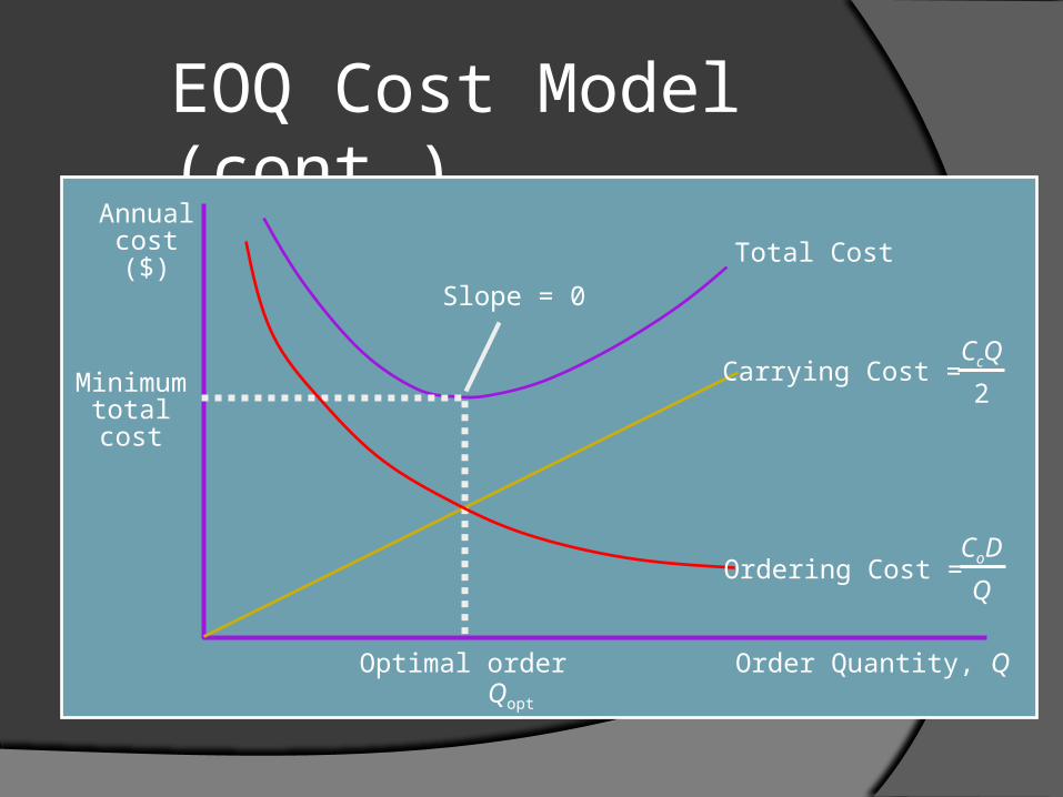
EOQ Cost Model (cont.)

Order Quantity, Q

Annual cost ($) Total Cost

Carrying Cost =CcQ

2

Slope = 0

Minimum total cost

Optimal order Qopt

Ordering Cost =CoD

Q

EOQ Example

Cc = $0.75 per yard Co = $150 D = 10,000 yards

Qopt =2CoD

Cc

Qopt =2(150)(10,000)

(0.75)

Qopt = 2,000 yards

TCmin = +CoD

Q

CcQ

2

TCmin = +(150)(10,000)

2,000

(0.75)(2,000)

2

TCmin = $750 + $750 = $1,500

Orders per year = D/Qopt

= 10,000/2,000

= 5 orders/year

Order cycle time = 311 days/(D/Qopt)

= 311/5

= 62.2 store days

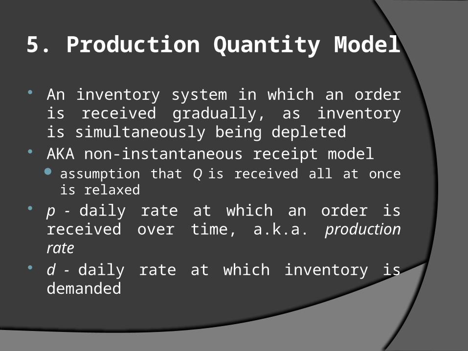
5. Production Quantity Model An inventory system in which an order is

received gradually, as inventory is simultaneously being depleted

AKA non-instantaneous receipt modelassumption that Q is received all at once is

relaxed p - daily rate at which an order is received

over time, a.k.a. production rate d - daily rate at which inventory is

demanded

Production Quantity Model (cont.)

Q(1-d/p)

Inventorylevel

(1-d/p)Q2

Time0

Orderreceipt period

Beginorder

receipt

Endorder

receipt

Maximuminventory level

Averageinventory level

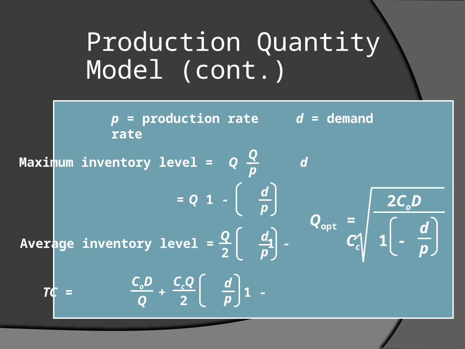
Production Quantity Model (cont.)

p = production rate d = demand rate

Maximum inventory level = Q - d

= Q 1 -

Qp

dp

Average inventory level = 1 -Q2

dp

TC = + 1 -dp

CoD

Q

CcQ

2

Qopt =2CoD

Cc 1 - dp

Production Quantity Model: Example

Cc = $0.75 per yard Co = $150 D = 10,000 yards

d = 10,000/311 = 32.2 yards per day p = 150 yards per day

Qopt = = = 2,256.8 yards

2CoD

Cc 1 - dp

2(150)(10,000)

0.75 1 - 32.2150

TC = + 1 - = $1,329dp

CoD

Q

CcQ

2

Production run = = = 15.05 days per orderQp

2,256.8150

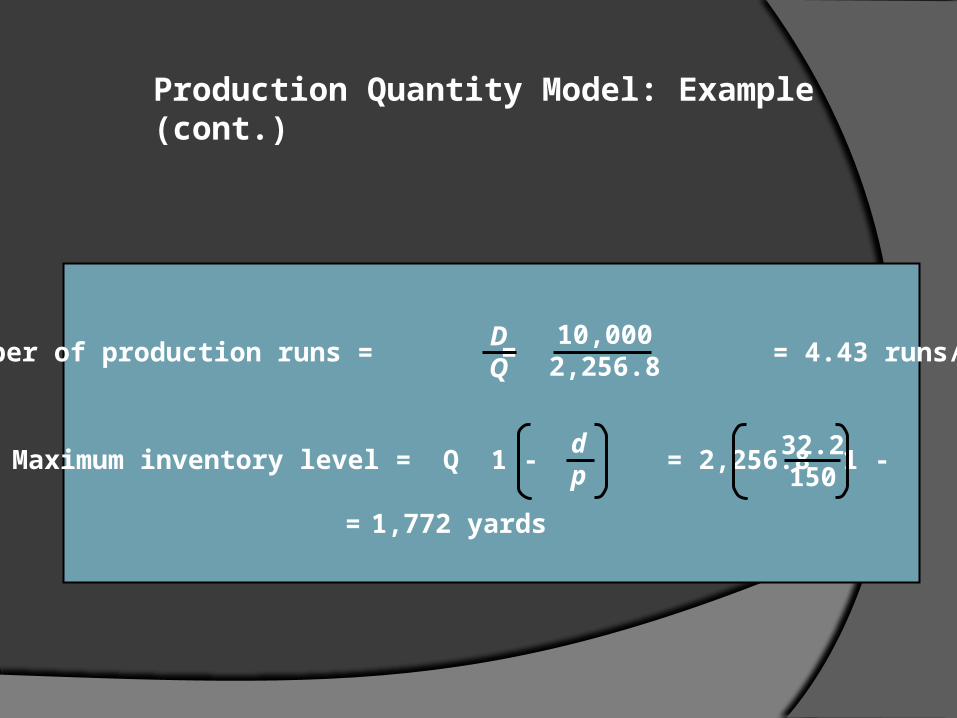
Production Quantity Model: Example (cont.)

Number of production runs = = = 4.43 runs/yearDQ

10,0002,256.8

Maximum inventory level = Q 1 - = 2,256.8 1 -

= 1,772 yards

dp

32.2150

6. QUANTITY DISCOUNTS

Price per unit decreases as order quantity increases

TC = + + PDCoD

Q

CcQ

2

where

P = per unit price of the itemD = annual demand

Quantity Discount Model (cont.)

Qopt

Carrying cost

Ordering cost

Inve

ntor

y co

st (

$)

Q(d1 ) = 100 Q(d2 ) = 200

TC (d2 = $6 )

TC (d1 = $8 )

TC = ($10 ) ORDER SIZE PRICE0 - 99 $10100 – 199 8 (d1)200+ 6 (d2)

Quantity Discount: Example

QUANTITY PRICE

1 - 49 $1,400

50 - 89 1,100

90+ 900

Co = $2,500

Cc = $190 per computer

D = 200

Qopt = = = 72.5 PCs2CoD

Cc

2(2500)(200)190

TC = + + PD = $233,784 CoD

Qopt

CcQopt

2

For Q = 72.5

TC = + + PD = $194,105CoD

Q

CcQ

2

For Q = 90

7. ABC ANALYSIS The materials are divided in to a number of categories

for adopting a selective approach for material control.

Classification of items as a, b, or c

Purpose: set priorities for management attention. ‘A’ items: 20% of the items contributes, 80% value ‘B’ items: 30 % of Items contributes , 15% Value ‘C’ items: 50 % of Items contributes , 5% value Three classes is arbitrary; could be any number. Percents are approximate.

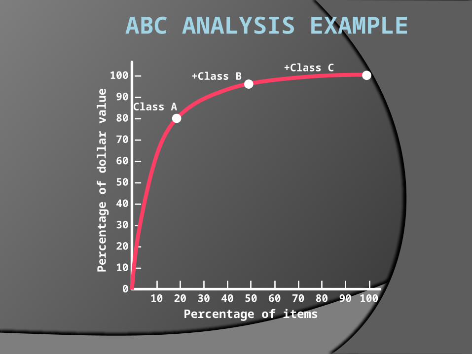
ABC ANALYSIS EXAMPLE

10 20 30 40 50 60 70 80 90 100

Percentage of items

Per

cen

tag

e o

f d

oll

ar v

alu

e

100 —

90 —

80 —

70 —

60 —

50 —

40 —

30 —

20 —

10 —

0 —

+Class C

Class A

+Class B

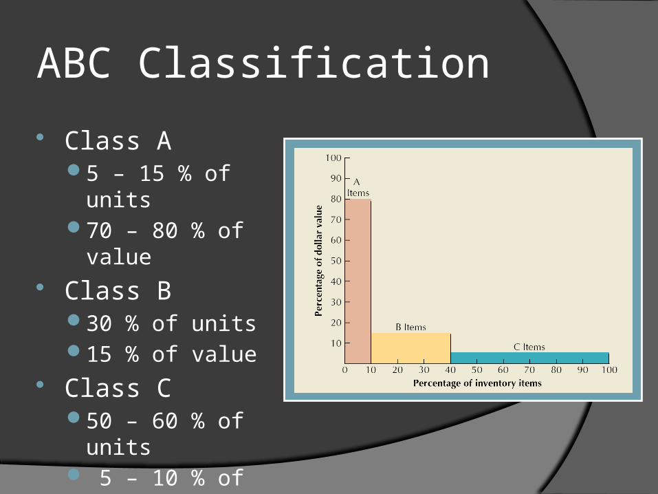
ABC Classification

Class A5 – 15 % of units70 – 80 % of value

Class B30 % of units15 % of value

Class C50 – 60 % of units 5 – 10 % of value

8. JIT CONTROL SYSTEM

Just in Time purchasing is the purchase of material in such a way that delivery of purchased items is assured before their use or demand.

9. VED Analysis

VED – Vital, Essential, Desirable – analysis is used primarily for control of spare parts. The spare, parts can be divided into three categories – vital, essential or desirable – keeping in view the critically to production.

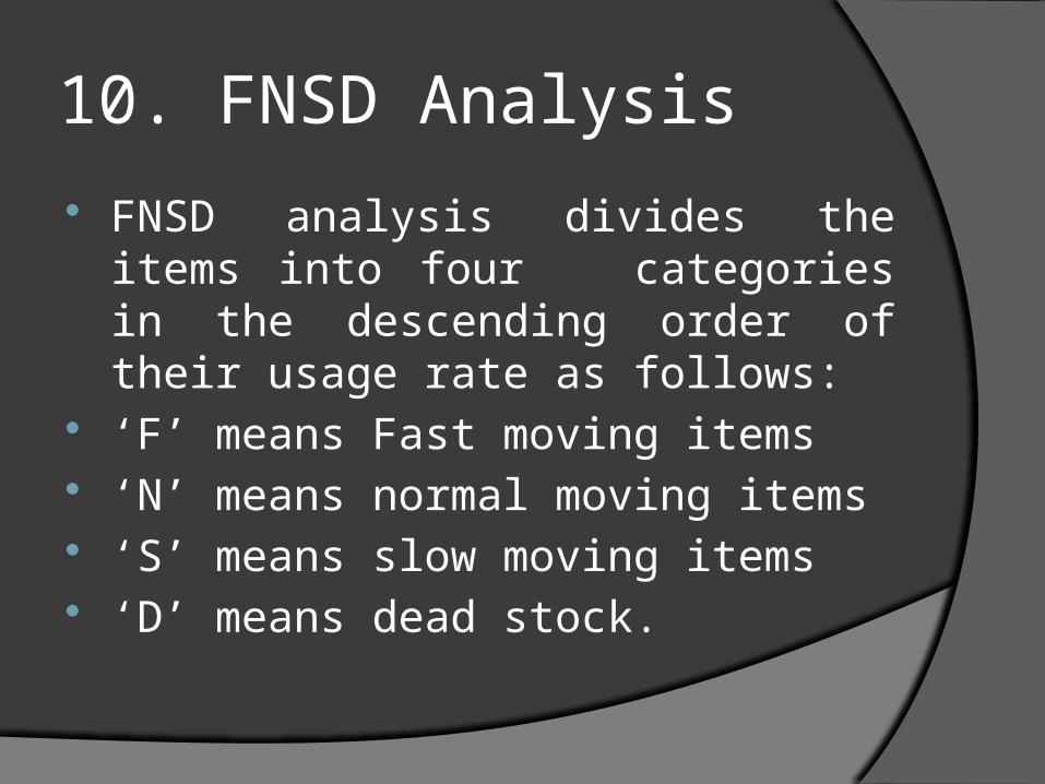
10. FNSD Analysis

FNSD analysis divides the items into four categories in the descending order of their usage rate as follows:

‘F’ means Fast moving items ‘N’ means normal moving items ‘S’ means slow moving items ‘D’ means dead stock.

11. Perpetual Inventory System Perpetual Inventory is a system of records maintained

by the controlling department, which reflects the physical movement of stocks and their current balance. It aims at devising the system of records by which the receipts and issues of stores may be recorded immediately at the time of each transaction and the balance may be brought out so as to show the up-to-date position.

 

The records used for perpetual inventory are:

(i) Bin Cards;

(ii) Store Ledger Accounts or Stores Record cards;

(iii) The forms and documents used for receipt, issue and transfer of materials.