Inventory Management

Inventory

• Raw material Inventory• Work in process Inventory• Finished product Inventory

• It is one of the dominant costs• Goal of effective inventory management in SC is

to have correct inventory at right place at right time to minimize system costs while satisfying customer service requirements

Inventory is held due to:• Unexpected changes in Customer Demand (due

to short life cycle of products thereby having no historical data of customer demand & many competing products)

• Many a times significant uncertainty in quantity and quality of supply, supplier costs, delivery times

• Lead times• Economies of Scale offered by transportation

Companies

An Effective Inventory Policy needs to consider:

• Customer Demand (may be known in advance or random, if random forecasting tools used to estimate average demand & variability in demand based on historical data)

• Replenishment Lead time• No. of different products (compete on budget/space)• Length of planning horizon• Costs

Order Costs (product & transportation cost) Inventory Holding Costs (state & property

taxes,insurance,maintenance costs,obsolescence costs,opportunity costs)

• Service level Requirements

Single Stage Inventory Control

(Inventory Management in a Single Supply chain Stage)

(Constant Demand for a single item)

Economic Lot Size Model (Ford W.Harris)

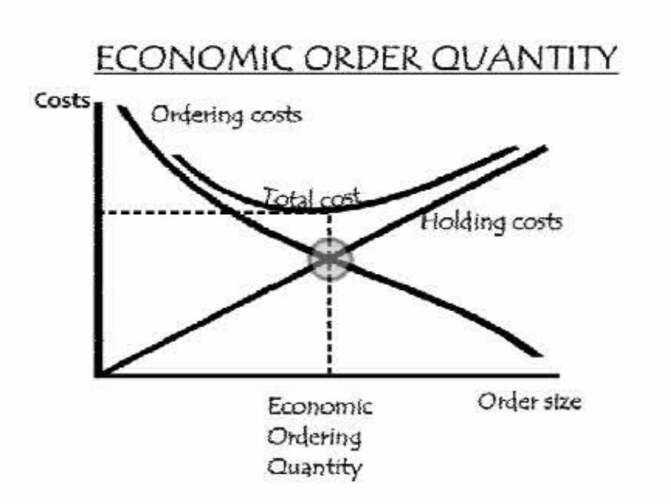
• Illustrates trade-offs between ordering and storage costs

Assumptions:• Constant demand @ ‘D’ items/day• Fixed order quantities @ ‘Q’ items/order• A fixed cost(setup) ‘K’ incurred everytime warehouse places an

order• An inventory carrying cost/holding cost ‘h’ per unit/day• Zero Lead time• Zero initial inventory• Long (infinite) planning horizon

Goal is to find optimal order policy that minimizes annual purchasing and carrying costs while meeting all demand

• Consider Inventory level as a function of time• Total inventory cost in a cycle of length T is

K+ hTQ/2K: fixed cost charged once per orderh: per unit per time period holding costT: length of cycleQ/2: average inventory levelAlso, Q=TDSo, average total cost per unit time:

KD/Q + hQ/2

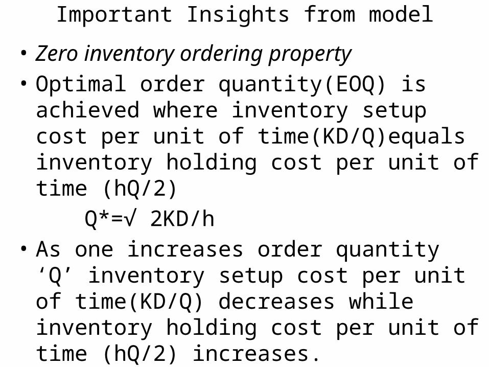
Important Insights from model

• Zero inventory ordering property• Optimal order quantity(EOQ) is achieved where

inventory setup cost per unit of time(KD/Q)equals inventory holding cost per unit of time (hQ/2)

Q*=√ 2KD/h• As one increases order quantity ‘Q’ inventory

setup cost per unit of time(KD/Q) decreases while inventory holding cost per unit of time (hQ/2) increases.

• While total inventory cost is insensitive to order quantities (Q=bQ*)

Effect of Demand Uncertainty

Principles of all forecasts:1. Forecast is always wrong (difficult to match

supply & demand)2. Longer the forecast horizon, worse the forecast

(difficult to predict customer demand for a long period of time)

3. Aggregate forecasts are more accurate (easier to predict demand across all SKUs within one product family, an example of risk pooling)

Single Period Model

• To understand impact of demand uncertainty• Consider a product that has short lifecycle and hence firm has only one

ordering opportunity(ex. Swimsuits)Inferences:• Optimal order qty. is not necessarily equal to forecast/average demand.

Rather it depends on relationship between marginal profit achieved from selling an additional unit and marginal cost.

If an additional unit is sold:• MP= SP /unit – variable ordering(production) cost/unitIf an additional unit is not sold:• MC= variable ordering(production) cost/unit – salvage value/unit• If MC> MP, then optimal quantity in general will be less than average

demand• Risk/Reward tradeoff: With increase in production qty risk/probability of

large losses and probability of large gains increases.

Initial Inventory

• Firm already has some inventory of product in hand,may be of previous season

• Trade off is between having a limited amount of inventory by avoiding paying fixed cost vs. paying fixed cost and having higher inventory level.

• Min max policy or (s,S): On reviewing if inventory level is below is certain value,s, we order/produce to increase the inventory to level,S. Where ‘s’ is referred as reorder point/min and ‘S’ is referred as order-up-to level/max

Multiple Order Opportunities(Random demand, Repeated orders)

When demand is random, distributor has to hold inventory due to following reasons:

• To satisfy demand occurring during lead times• To protect against uncertainty in demand• To balance annual inventory holding costs and

annual fixed order costsTwo type of Policies: • Continous Review Policy• Periodic Review Policy

Continous Review Policy

Inventory is reviewed continuously & order is placed when inventory reaches a particular level or reorder point

Assumptions:• Daily demand is random & follows a normal distribution• Every time distributor places order from manufacturer,distributor

pays a fixed cost,K, plus an amount proportional to quantity ordered

• Inventory holding cost is charged per item per unit time• After continuous review if an order is placed order arrives after

appropriate lead time• If a customer order arrives when there is no inventory in

hand(distributor is stocked out), order is lost• Distributor specifies a reqd. service level (service level is the

probability of not stocking out during lead time)•

• AVG=average daily demand• STD= Standard deviation of daily demand faced

by distributor• L= Replenishment Lead time• h= cost of holding one unit for one day• α= service level

(probability of stocking out is 1- α)

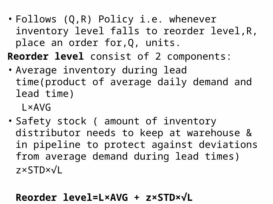
• Follows (Q,R) Policy i.e. whenever inventory level falls to reorder level,R, place an order for,Q, units.

Reorder level consist of 2 components:• Average inventory during lead time(product of

average daily demand and lead time) L×AVG

• Safety stock ( amount of inventory distributor needs to keep at warehouse & in pipeline to protect against deviations from average demand during lead times)

z×STD×√L

Reorder level=L×AVG + z×STD×√L

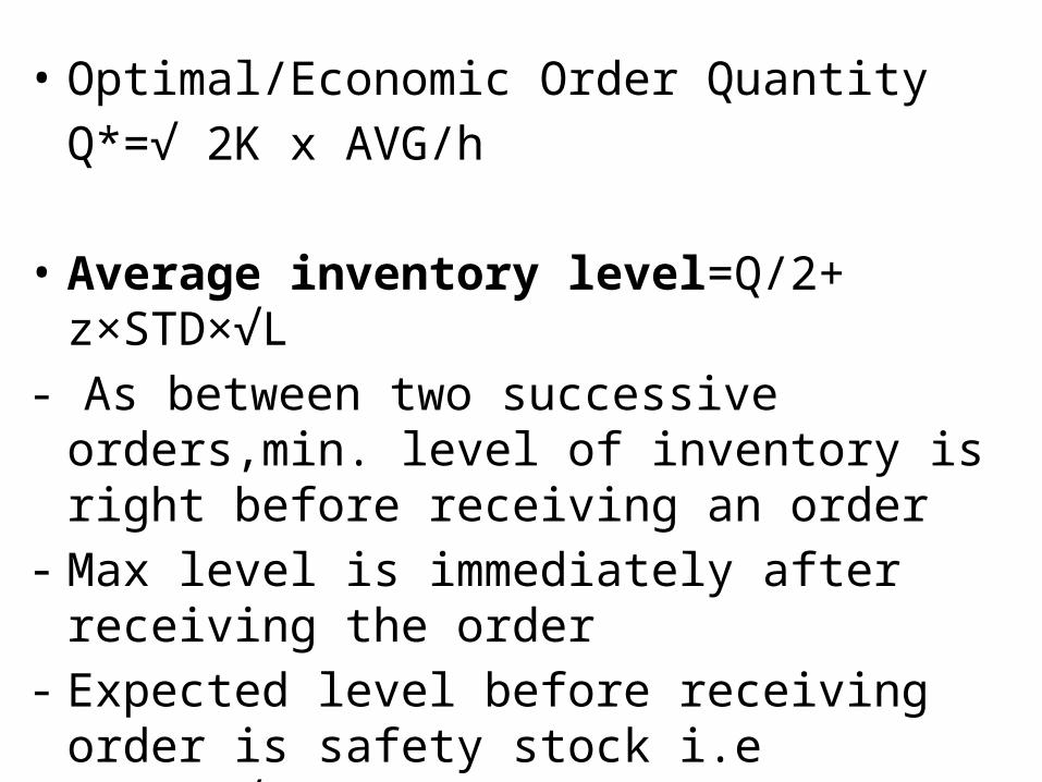
• Optimal/Economic Order QuantityQ*=√ 2K x AVG/h

• Average inventory level=Q/2+ z×STD×√L- As between two successive orders,min. level of

inventory is right before receiving an order- Max level is immediately after receiving the order- Expected level before receiving order is safety

stock i.e z×STD×√L- Expected Level immediately after receiving order

Q+ z×STD×√L

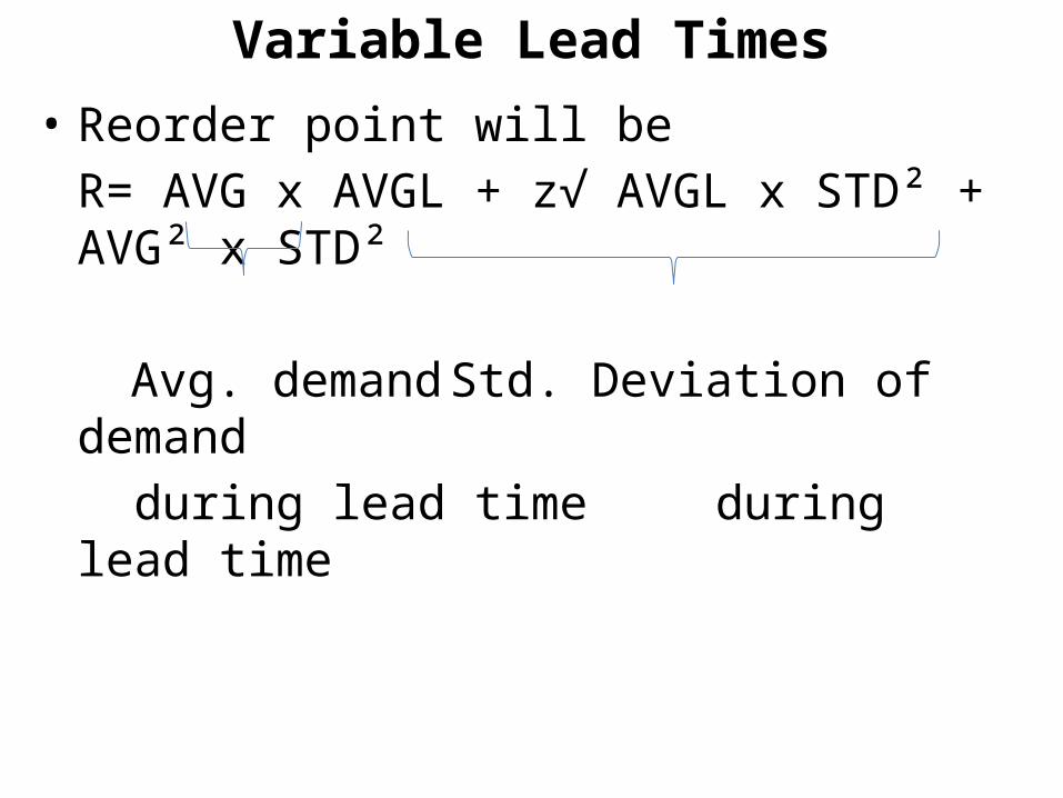
Variable Lead Times• Reorder point will be

R= AVG x AVGL + z√ AVGL x STD² + AVG² x STD²

Avg. demand Std. Deviation of demand during lead time during lead time

Periodic Review Policy

Inventory level is reviewed periodically at regular intervals and an appropriate quantity is ordered after each review

• In case of short intervals (daily), modified (Q,R) policy should be used i.e (s,S)policy where Q and R values are calculated as if it were a continuous review model and s is set equal to R and S equal to R+Q

• In case of long intervals, quantity is ordered after each review n then fixed cost of placing an order is sunk cost(zero). Presumably, fixed cost is used to determine the review interval

• So inventory policy (order quantity) is characterized by a single parameter i.e. base stock level (or target inventory level)

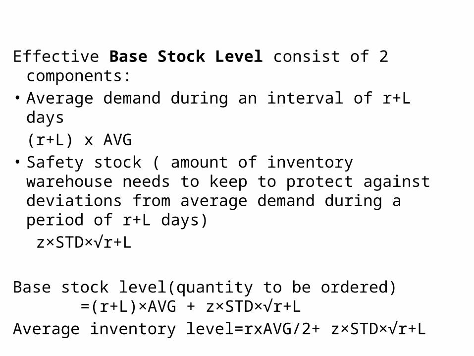
Effective Base Stock Level consist of 2 components:• Average demand during an interval of r+L days

(r+L) x AVG• Safety stock ( amount of inventory warehouse

needs to keep to protect against deviations from average demand during a period of r+L days)

z×STD×√r+L

Base stock level(quantity to be ordered) =(r+L)×AVG + z×STD×√r+L

Average inventory level=rxAVG/2+ z×STD×√r+L

Risk Pooling

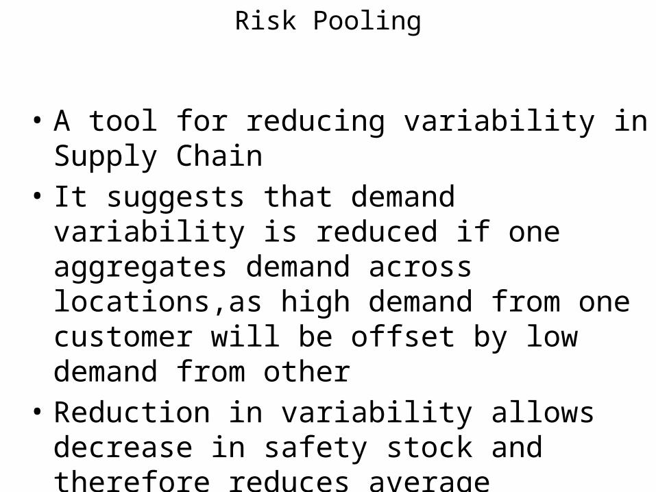
• A tool for reducing variability in Supply Chain• It suggests that demand variability is reduced if

one aggregates demand across locations,as high demand from one customer will be offset by low demand from other

• Reduction in variability allows decrease in safety stock and therefore reduces average inventory

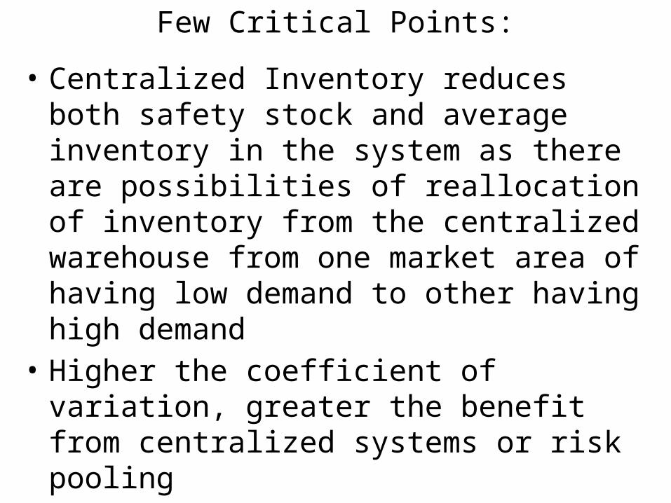
Few Critical Points:

• Centralized Inventory reduces both safety stock and average inventory in the system as there are possibilities of reallocation of inventory from the centralized warehouse from one market area of having low demand to other having high demand

• Higher the coefficient of variation, greater the benefit from centralized systems or risk pooling

• Benefit from risk pooling depends on behavior of demand from one market relative to other. It decreases if demand from both is showing very high positive correlation

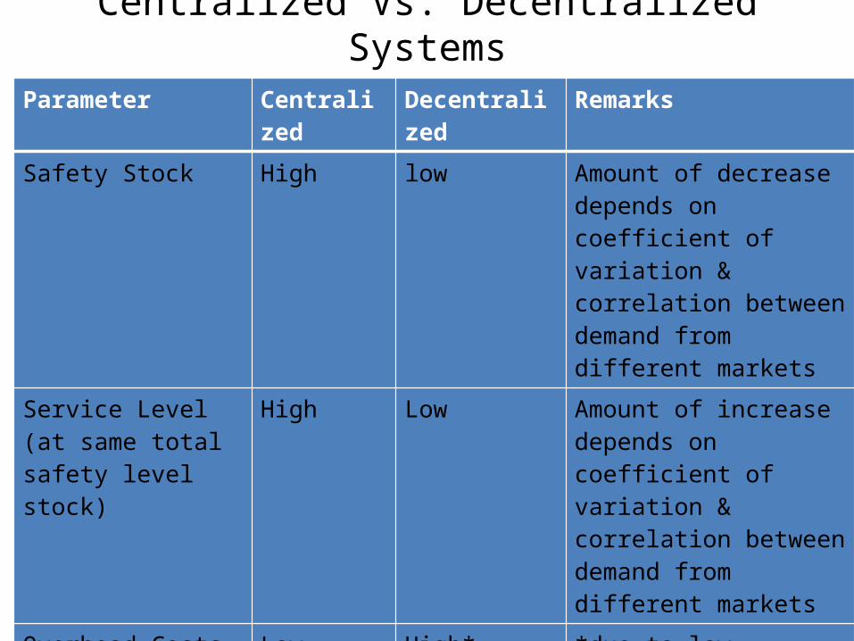
Centralized Vs. Decentralized Systems

Parameter Centralized Decentralized Remarks

Safety Stock High low Amount of decrease depends on coefficient of variation & correlation between demand from different markets

Service Level (at same total safety level stock)

High Low Amount of increase depends on coefficient of variation & correlation between demand from different markets

Overhead Costs Low High* *due to low economies of scale

Customer Lead Time High Low

Transportation CostOutboundInbound

HighLow

LowHigh