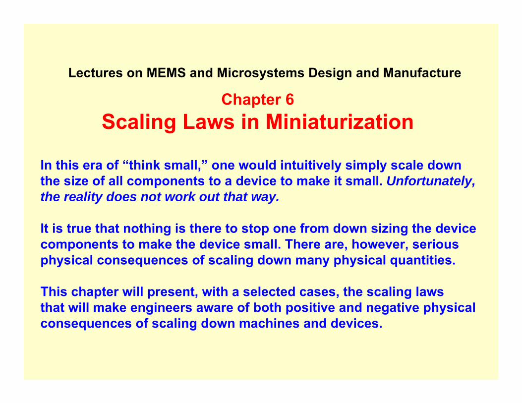
Chapter 6Scaling Laws in Miniaturization

In this era of “think small,” one would intuitively simply scale down the size of all components to a device to make it small. Unfortunately, the reality does not work out that way.

It is true that nothing is there to stop one from down sizing the device components to make the device small. There are, however, seriousphysical consequences of scaling down many physical quantities.

This chapter will present, with a selected cases, the scaling laws that will make engineers aware of both positive and negative physical consequences of scaling down machines and devices.

Lectures on MEMS and Microsystems Design and Manufacture

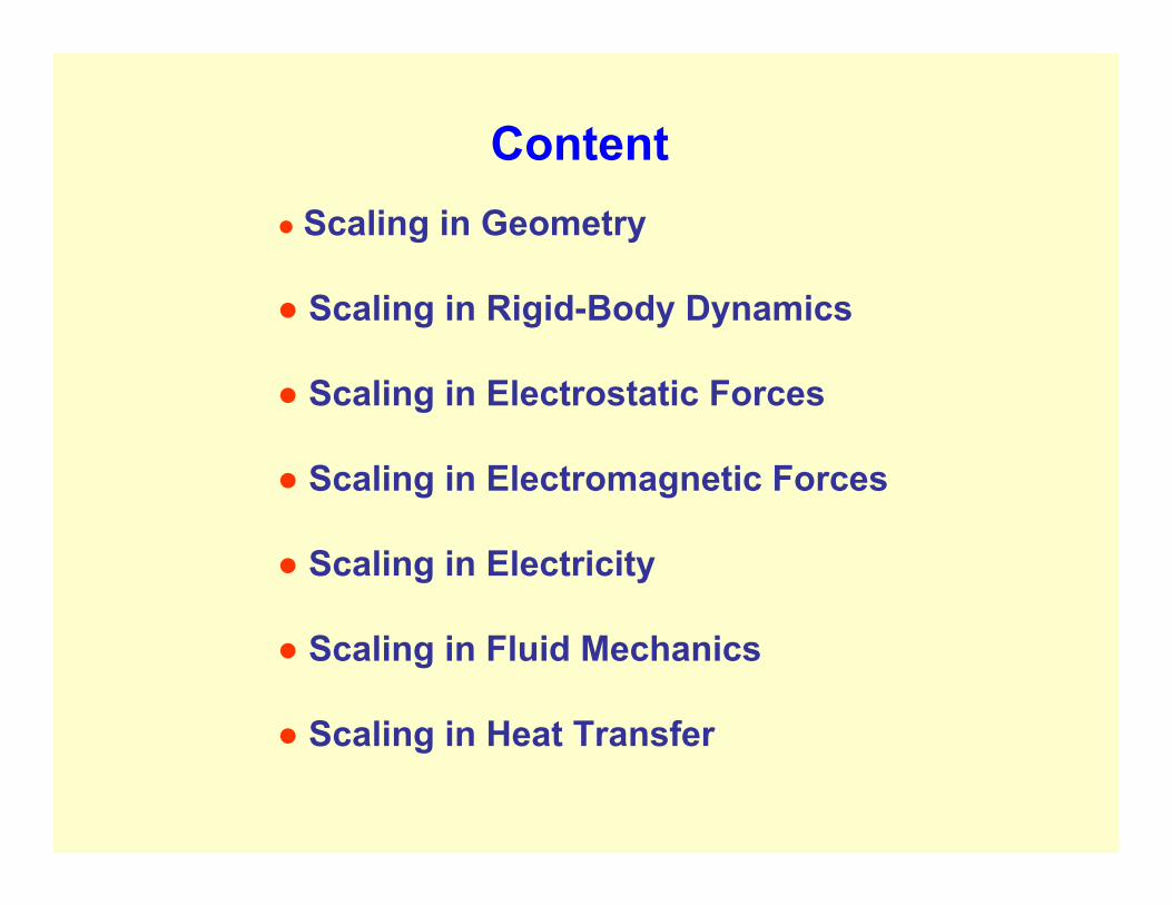
● Scaling in Geometry

● Scaling in Rigid-Body Dynamics

● Scaling in Electrostatic Forces

● Scaling in Electromagnetic Forces

● Scaling in Electricity

● Scaling in Fluid Mechanics

● Scaling in Heat Transfer

Content

WHY SCALING LAWS?Miniaturizing machines and physical systems is an ongoing effort in human civilization.

This effort has been intensified in recent years as market demands for:

Intelligent, Robust, Multi-functional and Low cost

consumer products has become more strong than ever.

The only solution to produce these consumer products is to package many components into the product –

making it necessary to miniaturize each individual components.

Miniaturization of physical systems is a lot more than just scaling down device components in sizes.

Some physical systems either cannot be scaled down favorably, or cannot be scaled down at all!

Scaling laws thus become the very first thing

that any engineer would do in the design of

MEMS and microsystems.

Types of Scaling Laws

1. Scaling in Geometry:

Scaling of physical size of objects

2. Scaling of Phenomenological Behavior

Scaling of both size and materialcharacterizations

Scaling in Geometry

● Volume (V) and surface (S) are two physical parameters that are frequently involved in machine design.

● Volume leads to the mass and weight of device components.

● Volume relates to both mechanical and thermal inertia. Thermal inertia is a measure on how fast we can heat or cool a solid. It is an important parameter in the design of a thermally actuated device as described in Chapter 5.

● Surface is related to pressure and the buoyant forces in fluid mechanics. For instance, surface pumping by using piezoelectric means is a practical way for driving fluids flow in capillary conduits.

When the physical quantity is to be miniaturized, the design engineer must weigh the magnitudes of the possible consequences from the reduction on both the volume and surface of the particular device.

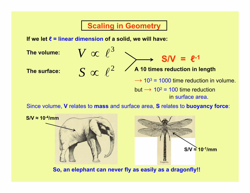
Scaling in GeometryIf we let ℓ = linear dimension of a solid, we will have:

The volume: 3l∝VThe surface: 2l∝S

S/V = ℓ-1

A 10 times reduction in length

→ 103 = 1000 time reduction in volume.but → 102 = 100 time reduction

in surface area.Since volume, V relates to mass and surface area, S relates to buoyancy force:

S/V ≈ 10-4/mm

S/V ≈ 10-1/mm

So, an elephant can never fly as easily as a dragonfly!!

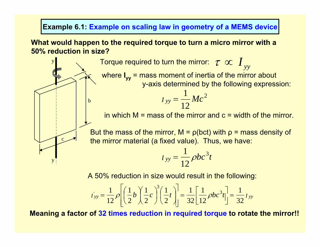
Example 6.1: Example on scaling law in geometry of a MEMS device

What would happen to the required torque to turn a micro mirror with a 50% reduction in size?

t

b

c

y

y

Torque required to turn the mirror: yyI∝τwhere Iyy = mass moment of inertia of the mirror about

y-axis determined by the following expression:2

121 McI yy =

in which M = mass of the mirror and c = width of the mirror.

But the mass of the mirror, M = ρ(bct) with ρ = mass density of the mirror material (a fixed value). Thus, we have:

tbcI yy3

121 ρ=

A 50% reduction in size would result in the following:

II yyyy tbctcb321

121

321

21

21

21

121 3

3' =⎥⎦

⎤⎢⎣⎡=

⎥⎥⎦

⎤

⎢⎢⎣

⎡⎟⎠⎞

⎜⎝⎛

⎟⎠⎞

⎜⎝⎛⎟⎠⎞

⎜⎝⎛= ρρ

Meaning a factor of 32 times reduction in required torque to rotate the mirror!!

Scaling in Rigid-Body Dynamics

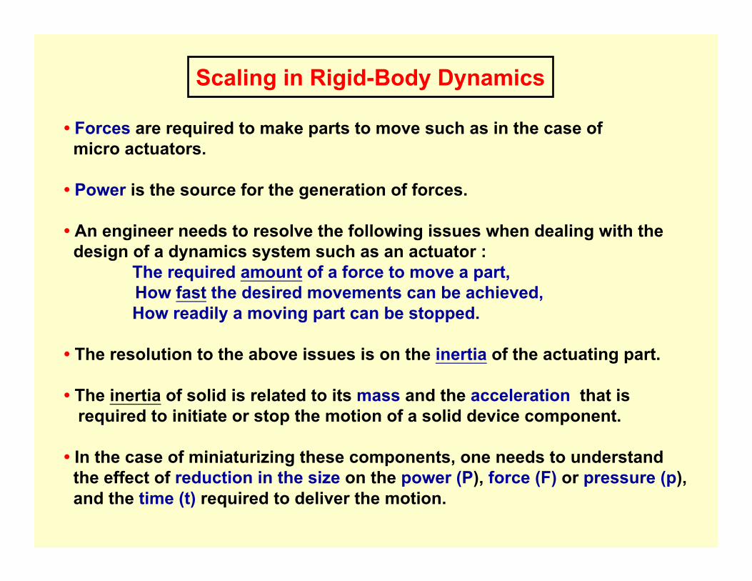
• Forces are required to make parts to move such as in the case ofmicro actuators.

• Power is the source for the generation of forces.

• An engineer needs to resolve the following issues when dealing with thedesign of a dynamics system such as an actuator :

The required amount of a force to move a part, How fast the desired movements can be achieved, How readily a moving part can be stopped.

• The resolution to the above issues is on the inertia of the actuating part.

• The inertia of solid is related to its mass and the acceleration that is required to initiate or stop the motion of a solid device component.

• In the case of miniaturizing these components, one needs to understand the effect of reduction in the size on the power (P), force (F) or pressure (p), and the time (t) required to deliver the motion.

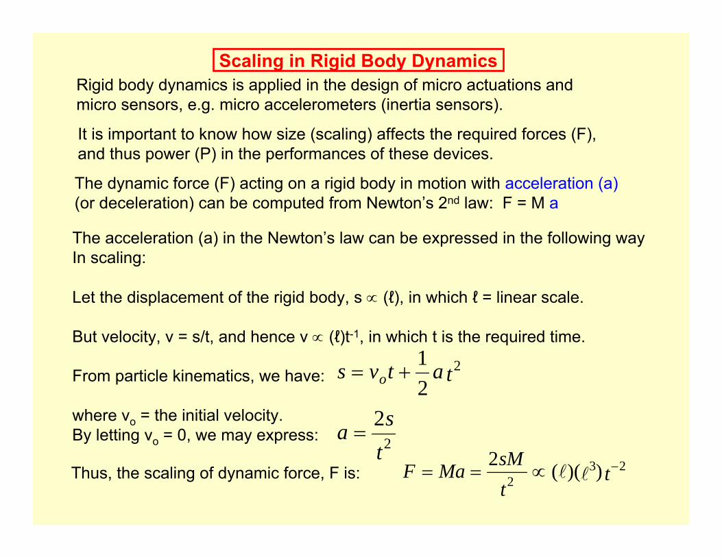
Scaling in Rigid Body DynamicsRigid body dynamics is applied in the design of micro actuations andmicro sensors, e.g. micro accelerometers (inertia sensors).

It is important to know how size (scaling) affects the required forces (F),and thus power (P) in the performances of these devices.

The acceleration (a) in the Newton’s law can be expressed in the following wayIn scaling:

Let the displacement of the rigid body, s ∝ (ℓ), in which ℓ = linear scale.

But velocity, v = s/t, and hence v ∝ (ℓ)t-1, in which t is the required time.

From particle kinematics, we have:

where vo = the initial velocity.By letting vo = 0, we may express:

The dynamic force (F) acting on a rigid body in motion with acceleration (a)(or deceleration) can be computed from Newton’s 2nd law: F = M a

tatvs o2

21

+=

tsa 2

2=

Thus, the scaling of dynamic force, F is: ttsMMaF 23

2 ))((2 −∝== ll

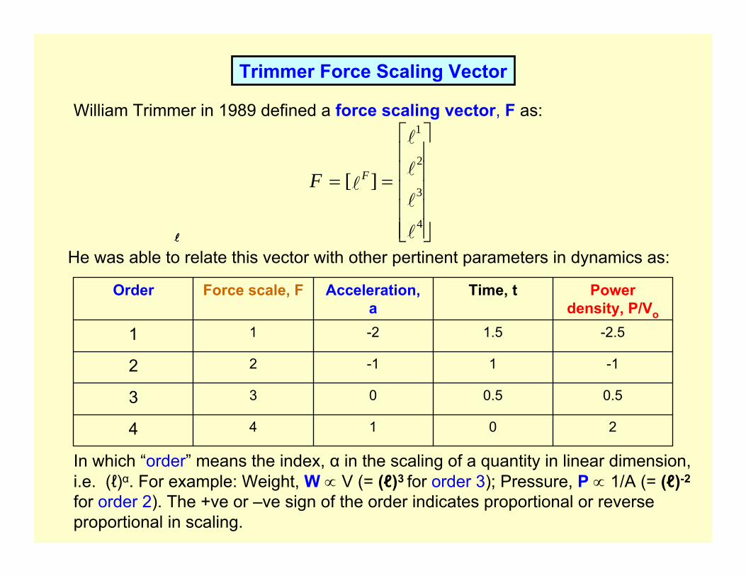
Trimmer Force Scaling Vector

William Trimmer in 1989 defined a force scaling vector, F as:

⎥⎥⎥⎥⎥

⎦

⎤

⎢⎢⎢⎢⎢

⎣

⎡

==

l

l

l

l

l

4

3

2

1

][ FF

He was able to relate this vector with other pertinent parameters in dynamics as:lllllll

20144

0.50.5033

-11-122

-2.51.5-211

Power density, P/Vo

Time, tAcceleration, a

Force scale, FOrder

In which “order” means the index, α in the scaling of a quantity in linear dimension,i.e. (ℓ)α. For example: Weight, W ∝ V (= (ℓ)3 for order 3); Pressure, P ∝ 1/A (= (ℓ)-2

for order 2). The +ve or –ve sign of the order indicates proportional or reverse proportional in scaling.

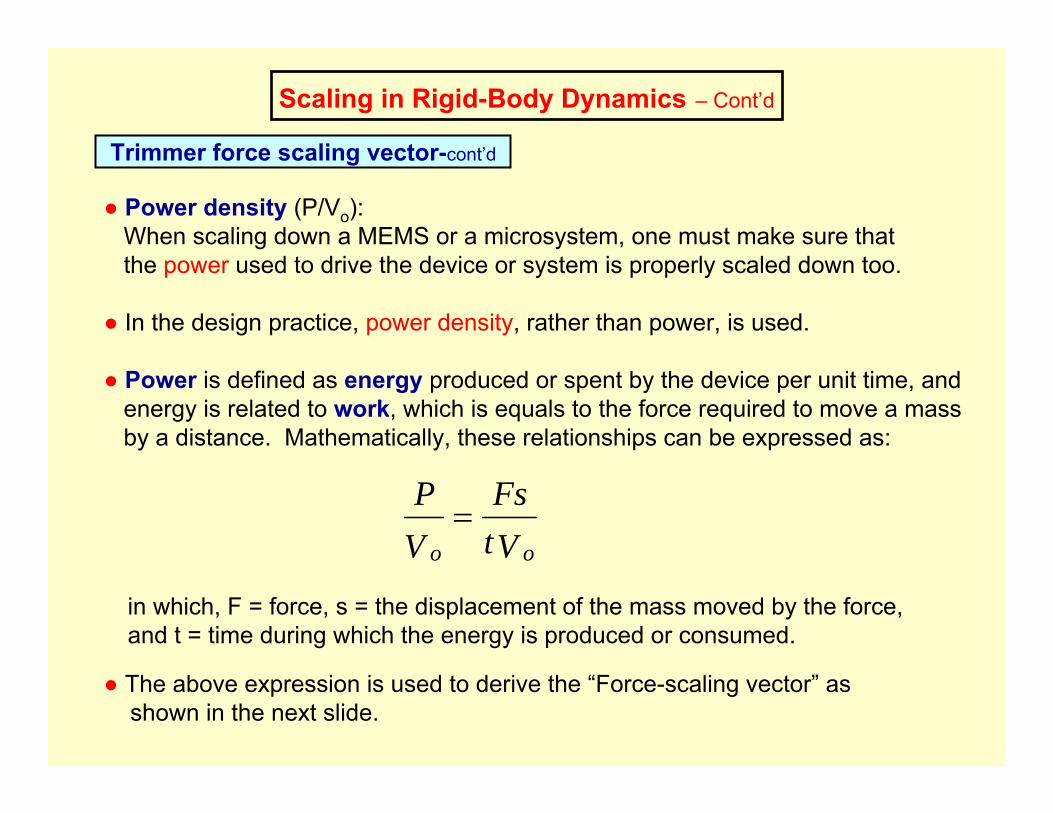
Scaling in Rigid-Body Dynamics – Cont’d

Trimmer force scaling vector-cont’d

● Power density (P/Vo):When scaling down a MEMS or a microsystem, one must make sure that the power used to drive the device or system is properly scaled down too.

● In the design practice, power density, rather than power, is used.

● Power is defined as energy produced or spent by the device per unit time, and energy is related to work, which is equals to the force required to move a mass by a distance. Mathematically, these relationships can be expressed as:

VtFs

VP

oo=

in which, F = force, s = the displacement of the mass moved by the force,and t = time during which the energy is produced or consumed.

● The above expression is used to derive the “Force-scaling vector” asshown in the next slide.

Scaling in Rigid-Body Dynamics – Cont’d

Trimmer force scaling vector-cont’d

⎥⎥⎥⎥⎥

⎦

⎤

⎢⎢⎢⎢⎢

⎣

⎡

=

⎥⎥⎥⎥⎥

⎦

⎤

⎢⎢⎢⎢⎢

⎣

⎡

=

===

−

−

−

−−

−

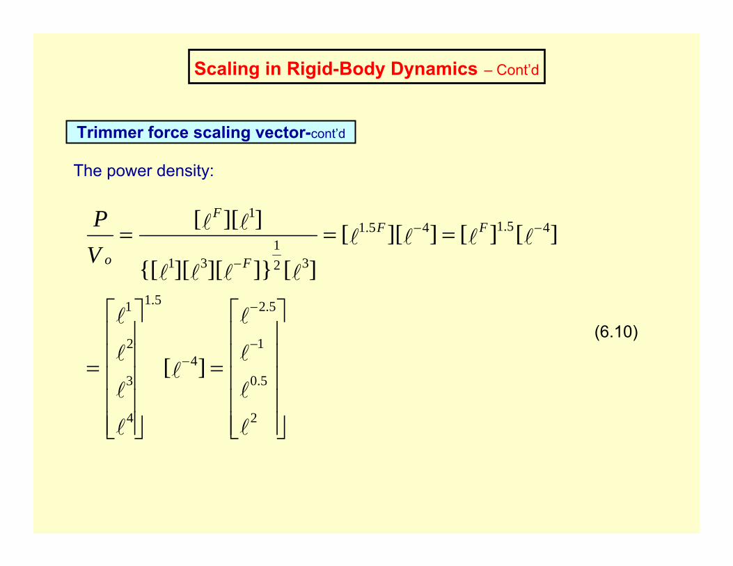
l

l

l

l

l

l

l

l

l

llll

llll

ll

2

5.0

1

5.2

4

5.1

4

3

2

1

45.145.1

321

31

1

][

][][]][[][]}][][{[

]][[ FF

F

F

oVP

(6.10)

The power density:

Example 6.2

Estimate the associate changes in the acceleration (a) and the time (t) and the power supply (P) to actuate a MEMS component if its weight is reduced by a factor of 10.

Solution:

Since W ∝ V (= (ℓ)3 , so it involves Order 3 scaling, from the table for scaling of dynamic forces, we get:

● There will be no reduction in the acceleration (ℓ0).

● There will be (ℓ0.5 ) = (10)0.5 = 3.16 reduction in the time to complete the motion.

● There will be (ℓ0.5) = 3.16 times reduction in power density (P/Vo).

The reduction of power consumption is 3.16 Vo. Since the volume of the component is reduced by a factor of 10, the power consumption after scaling down reduces by: P = 3.16/10 = 0.3 times.

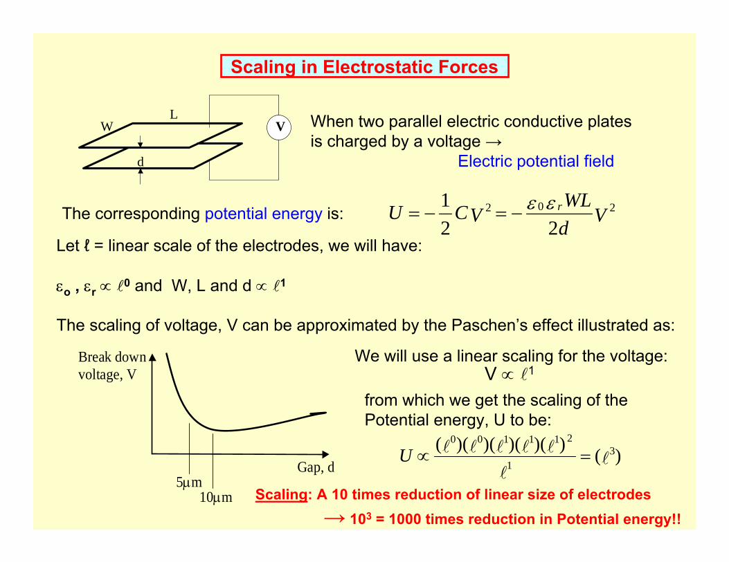
Scaling in Electrostatic Forces

V

d

LW When two parallel electric conductive plates

is charged by a voltage →Electric potential field

The corresponding potential energy is: VdWL

VCU r 202

221 εε−=−=

Let ℓ = linear scale of the electrodes, we will have:

εo , εr ∝ l0 and W, L and d ∝ l1

The scaling of voltage, V can be approximated by the Paschen’s effect illustrated as:

5µm10µm

Gap, d

Break downvoltage, V

We will use a linear scaling for the voltage:V ∝ l1

from which we get the scaling of the Potential energy, U to be:

)())()()()(( 31

211100

ll

lllll =∝U

Scaling: A 10 times reduction of linear size of electrodes→ 103 = 1000 times reduction in Potential energy!!

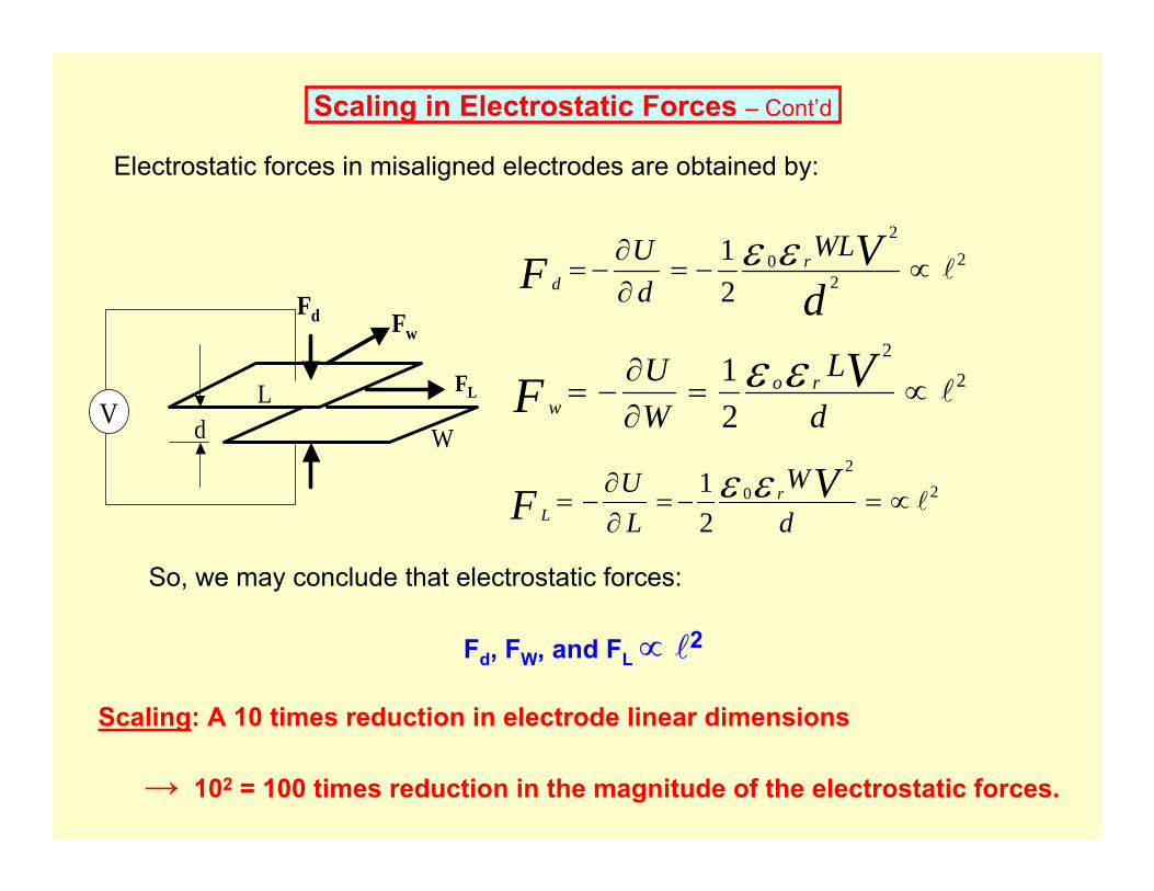
Scaling in Electrostatic Forces – Cont’d

Electrostatic forces in misaligned electrodes are obtained by:

WdL

Fd Fw

FLV

22

2

0

21

l∝−=∂∂

−=d

VFWL

dU r

dεε

22

21

l∝=∂∂

−=dL

WU VF ro

wεε

22

0

21

l∝=−=∂∂

−=dW

LU VF r

Lεε

So, we may conclude that electrostatic forces:

Fd, FW, and FL ∝ l2

Scaling: A 10 times reduction in electrode linear dimensions

→ 102 = 100 times reduction in the magnitude of the electrostatic forces.

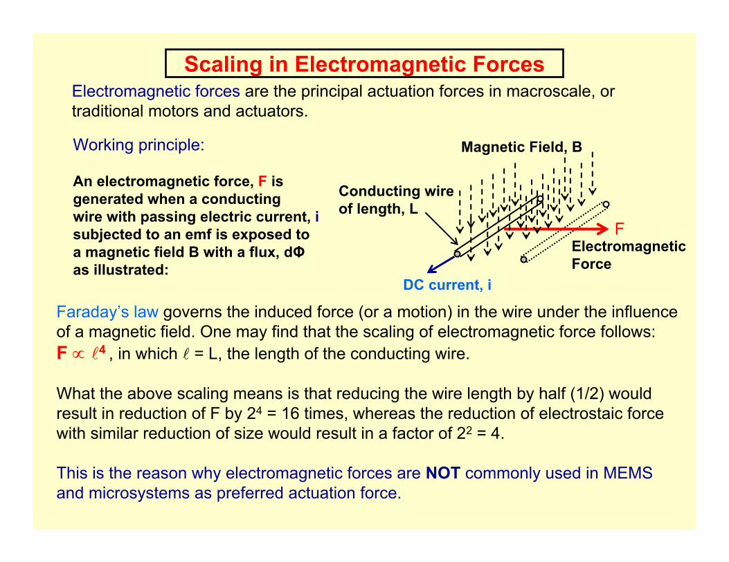
Scaling in Electromagnetic ForcesElectromagnetic forces are the principal actuation forces in macroscale, or traditional motors and actuators.

Magnetic Field, B

DC current, i

Electromagnetic Force

F

Conducting wireof length, L

Working principle:

An electromagnetic force, F is generated when a conducting wire with passing electric current, isubjected to an emf is exposed toa magnetic field B with a flux, dΦas illustrated:

Faraday’s law governs the induced force (or a motion) in the wire under the influence of a magnetic field. One may find that the scaling of electromagnetic force follows: F ∝ l4 , in which l = L, the length of the conducting wire.

What the above scaling means is that reducing the wire length by half (1/2) would result in reduction of F by 24 = 16 times, whereas the reduction of electrostaic force with similar reduction of size would result in a factor of 22 = 4.

This is the reason why electromagnetic forces are NOT commonly used in MEMS and microsystems as preferred actuation force.

Scaling in Electricity

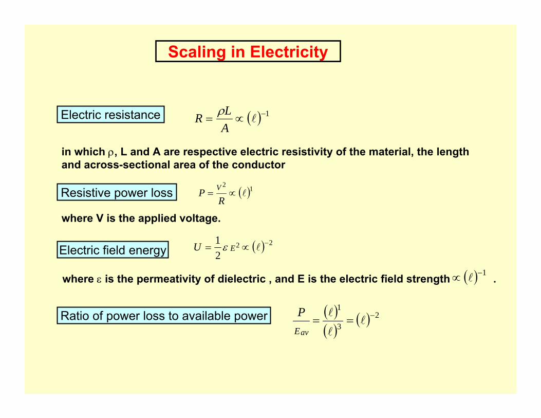
( ) 1−∝= lALR ρ

in which ρ, L and A are respective electric resistivity of the material, the length and across-sectional area of the conductor

Electric resistance

Resistive power loss ( )12

l∝=R

P V

where V is the applied voltage.

Electric field energy ( ) 2221 −∝= lEU ε

where ε is the permeativity of dielectric , and E is the electric field strength .( ) 1−∝ l

Ratio of power loss to available power ( )( )

( ) 23

1−== l

l

l

Eav

P

Scaling in Electricity

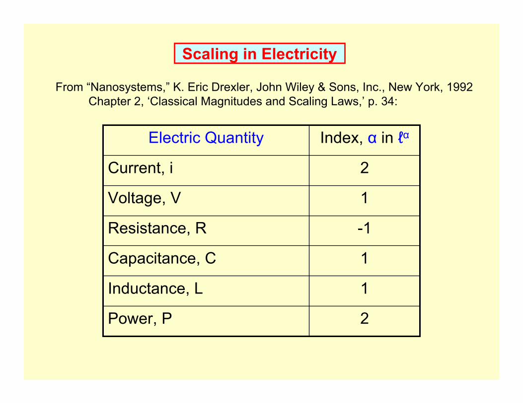
From “Nanosystems,” K. Eric Drexler, John Wiley & Sons, Inc., New York, 1992Chapter 2, ‘Classical Magnitudes and Scaling Laws,’ p. 34:

2Power, P

1Inductance, L

1Capacitance, C

-1Resistance, R

1Voltage, V

2Current, i

Index, α in ℓαElectric Quantity

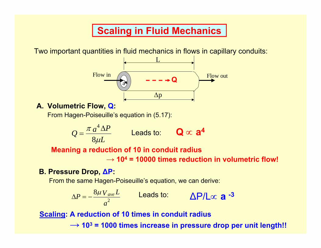
Scaling in Fluid Mechanics

Two important quantities in fluid mechanics in flows in capillary conduits:

LPaQ

µπ

8

4∆=

L

∆p

aFlow outFlow in

Q

Leads to: Q ∝ a4

Meaning a reduction of 10 in conduit radius → 104 = 10000 times reduction in volumetric flow!

A. Volumetric Flow, Q:From Hagen-Poiseuille’s equation in (5.17):

B. Pressure Drop, ∆P:From the same Hagen-Poiseuille’s equation, we can derive:

aLVP ave

28µ

−=∆ Leads to: ∆P/L∝ a -3

Scaling: A reduction of 10 times in conduit radius → 103 = 1000 times increase in pressure drop per unit length!!

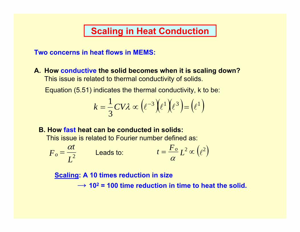
Scaling in Heat Conduction

Two concerns in heat flows in MEMS:

A. How conductive the solid becomes when it is scaling down?This issue is related to thermal conductivity of solids.Equation (5.51) indicates the thermal conductivity, k to be:

( )( )( ) ( )1313

31

llll =∝= −λCVk

B. How fast heat can be conducted in solids:This issue is related to Fourier number defined as:

Lt

Fo 2α

= Leads to: ( )l22 ∝= LFt o

α

Scaling: A 10 times reduction in size→ 102 = 100 time reduction in time to heat the solid.

End of Chapter 6