1

ME 310

Numerical Methods

Solving Systems of Linear Algebraic Equations

These presentations are prepared by

Dr. Cuneyt Sert

Mechanical Engineering Department

Middle East Technical University

Ankara, Turkey

csert@metu.edu.tr

They can not be used without the permission of the author

2

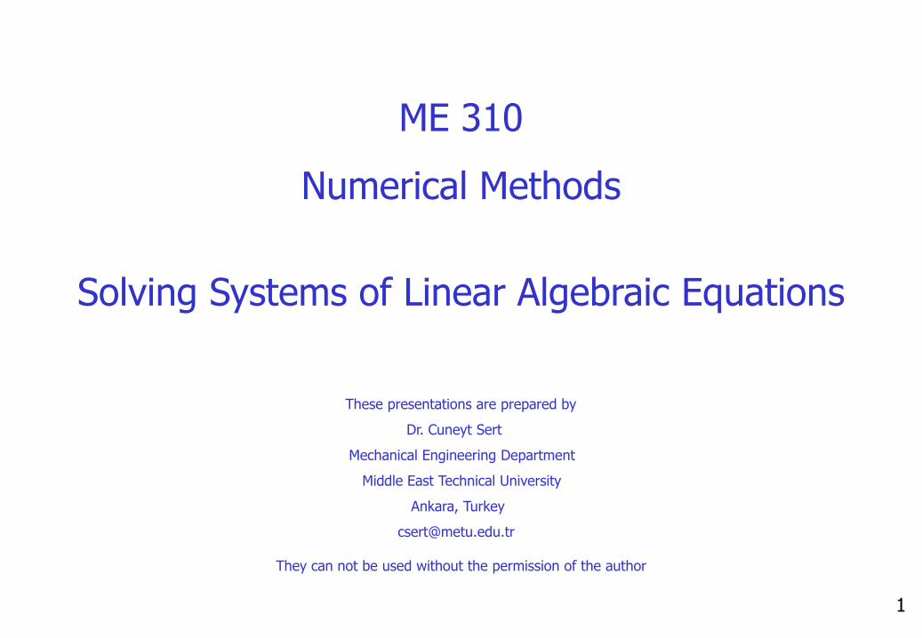
Math Introduction

f1(x1, x2, ..., xn) = 0

f2(x1, x2, ..., xn) = 0

...

fn(x1, x2, ..., xn) = 0

Linear Algebraic Equation: An equation of the form f(x)=0 where f is a polynomial with linear terms.

a11x1 + a12x2 + ... + a1nxn = b1

a21x1 + a22x2 + ... + a2nxn = b2

... ... ... ... an1x1 + an2x2 + ... + annxn = bn

Matrix Form: [A] {x} = {b}

[A] nxn Coefficient matrix

{x} nx1 Unknown vector{b} nx1 Right-Hand-Side (RHS) vector

A general set of equations.n equations, n unknowns.

A general set of linear algebraic equations.n equations, n unknowns.

3

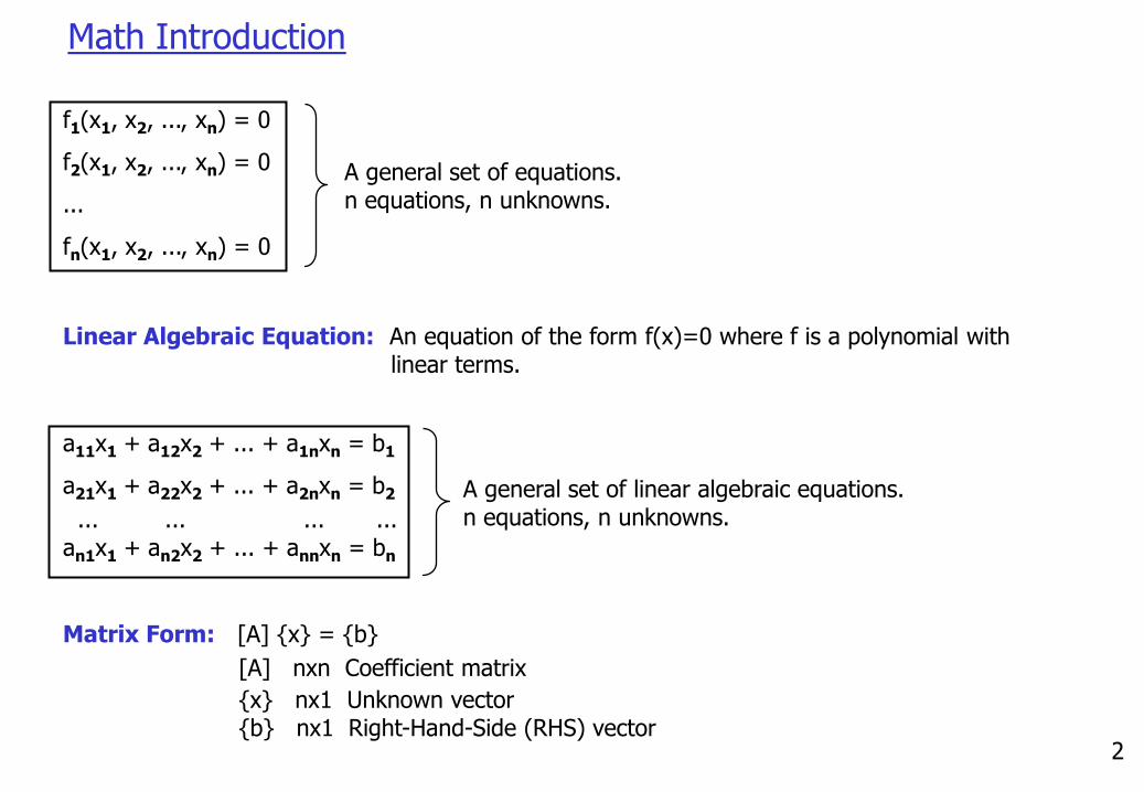
Review of Matrices

m n nm2n1n

m22221

m11211

aaa

aaa

aaa

]A[

2nd row

mth column

Elements are indicated by a i j

row column

Row vector: Column vector: n 1 n21 rrr]R[

1 m

m

2

1

c

c

c

]C[

Square matrix: [A]nxm is a square matrix if n=m. A system of n equations with n unknonws has a square coefficient matrix.

Main (principle) diagonal: of [A]nxn consists of elements aii ; i=1,...,n

Symmetric matrix: If aij = aji [A]nxn is a symmetric matrix

Diagonal matrix: [A]nxn is diagonal if aij = 0 for all i=1,...,n ; j=1,...,n and ij

Identity matrix: [A]nxn is an identity matrix if it is diagonal with aii=1 i=1,...,n . Shown as [I]

4

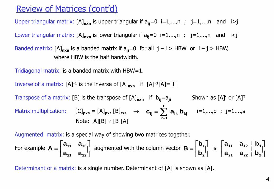
Upper triangular matrix: [A]nxn is upper triangular if aij=0 i=1,...,n ; j=1,...,n and i>j

Lower triangular matrix: [A]nxn is lower triangular if aij=0 i=1,...,n ; j=1,...,n and i<j

Banded matrix: [A]nxn is a banded matrix if aij=0 for all j – i > HBW or i – j > HBW,

where HBW is the half bandwidth.

Tridiagonal matrix: is a banded matrix with HBW=1.

Inverse of a matrix: [A]-1 is the inverse of [A]nxn if [A]-1[A]=[I]

Transpose of a matrix: [B] is the transpose of [A]nxn if bij=aji Shown as [A] or [A]T

Matrix multiplication: [C]pxs = [A]pxr [B]rxs i=1,...,p ; j=1,...,s

Note: [A][B] [B][A]

Augmented matrix: is a special way of showing two matrices together.

For example augmented with the column vector is

Determinant of a matrix: is a single number. Determinant of [A] is shown as |A|.

Review of Matrices (cont’d)

r

1k

kjikij b a c

2221

1211

aa

aaA

22221

11211

baa

baa

2

1

b

bB

5

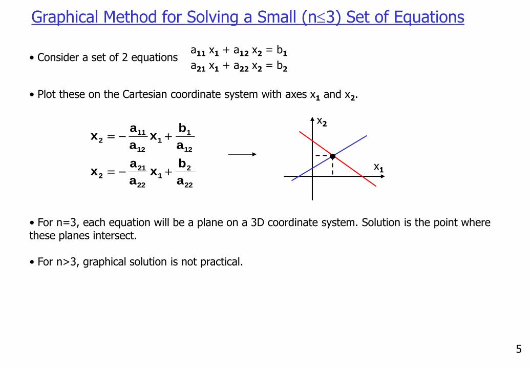
Graphical Method for Solving a Small (n3) Set of Equations

• Consider a set of 2 equationsa11 x1 + a12 x2 = b1

a21 x1 + a22 x2 = b2

• Plot these on the Cartesian coordinate system with axes x1 and x2.

22

21

22

212

12

11

12

112

a

bx

a

ax

a

bx

a

ax

• For n=3, each equation will be a plane on a 3D coordinate system. Solution is the point where these planes intersect.

• For n>3, graphical solution is not practical.

x1

x2

6

Graphical Method (cont’d)

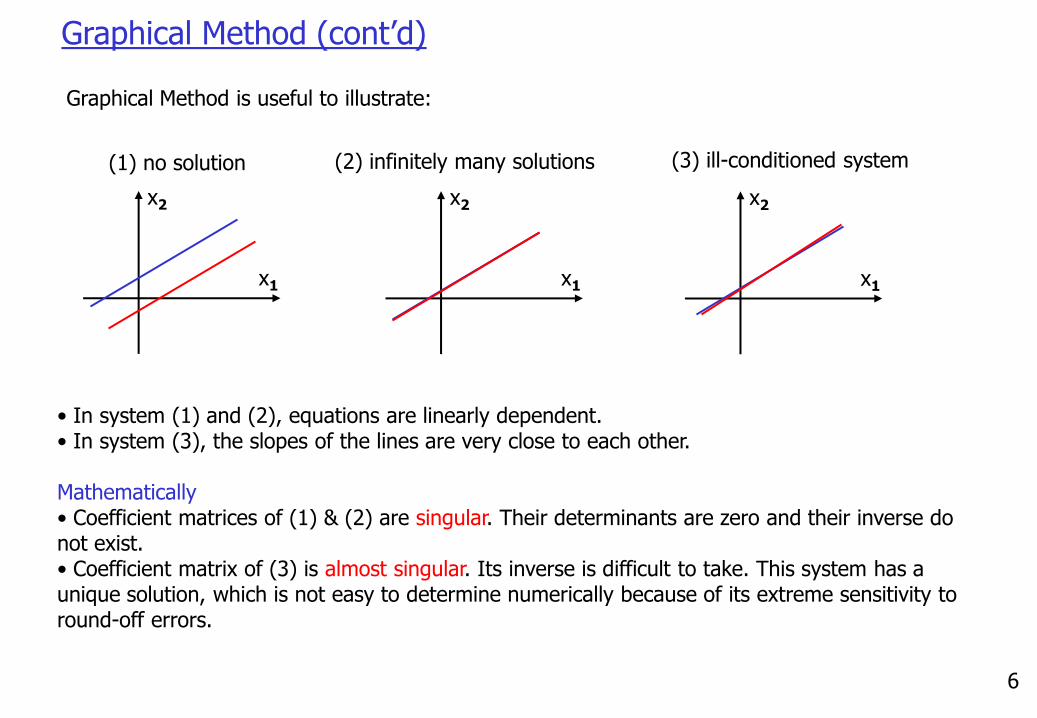
• In system (1) and (2), equations are linearly dependent.• In system (3), the slopes of the lines are very close to each other.

Mathematically• Coefficient matrices of (1) & (2) are singular. Their determinants are zero and their inverse do not exist.• Coefficient matrix of (3) is almost singular. Its inverse is difficult to take. This system has a unique solution, which is not easy to determine numerically because of its extreme sensitivity to round-off errors.

(1) no solution

x1

x2

x1

x2

(2) infinitely many solutions

x1

x2

(3) ill-conditioned system

Graphical Method is useful to illustrate:

7

Cramer’s Rule for Solving a Set of Equations

• Determinant of a 2x2 matrix is 21122211

2221

1211aaaa

aa

aaD

• Determinant of a 3x3 matrix is

3231

2221

13

3331

2321

12

3332

2322

11aa

aaa

aa

aaa

aa

aaaD

• Determinant of a general nxn matrix can be calculated recursively using the above pattern.

x1 - 3x2 = 5

2x1 - 6x2 = 7

• Determinant of an illl-conditioned system is close to zero.2x1 - 3x2 = 5

3.98x1 - 6x2 = 7

Warning: Multiply both equations of the above system with 100

This system is as ill-conditioned as the previous one but it has a determinant 10000 times larger. Therefore we need to scale a system when we talk about the magnitude of its determinant. Details will come later.

200x1 – 300x2 = 500

398x1 - 600x2 = 700

• Determinant of a singular system is zero.

Determinant of a system

8

Cramer’s Rule for Solving a Set of Equations (Cont’d)

For a 3x3 system D

baa

baa

baa

xD

aba

aba

aba

xD

aab

aab

aab

x33231

22221

11211

3

33331

23221

13111

2

33323

23222

13121

1

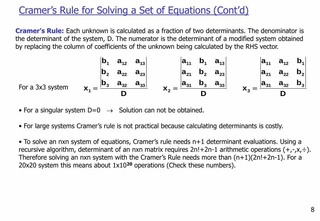
• For a singular system D=0 Solution can not be obtained.

• For large systems Cramer’s rule is not practical because calculating determinants is costly.

• To solve an nxn system of equations, Cramer’s rule needs n+1 determinant evaluations. Using a recursive algorithm, determinant of an nxn matrix requires 2n!+2n-1 arithmetic operations (+,-,x,÷). Therefore solving an nxn system with the Cramer’s Rule needs more than (n+1)(2n!+2n-1). For a 20x20 system this means about 1x1020 operations (Check these numbers).

Cramer’s Rule: Each unknown is calculated as a fraction of two determinants. The denominator is the determinant of the system, D. The numerator is the determinant of a modified system obtained by replacing the column of coefficients of the unknown being calculated by the RHS vector.

9

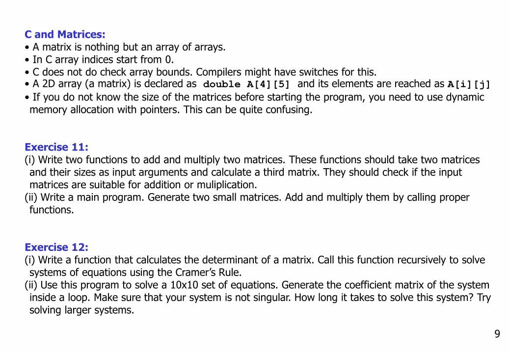
C and Matrices:• A matrix is nothing but an array of arrays.• In C array indices start from 0.• C does not do check array bounds. Compilers might have switches for this. • A 2D array (a matrix) is declared as double A[4][5] and its elements are reached as A[i][j]

• If you do not know the size of the matrices before starting the program, you need to use dynamic memory allocation with pointers. This can be quite confusing.

Exercise 11:(i) Write two functions to add and multiply two matrices. These functions should take two matrices and their sizes as input arguments and calculate a third matrix. They should check if the input matrices are suitable for addition or muliplication.

(ii) Write a main program. Generate two small matrices. Add and multiply them by calling proper functions.

Exercise 12:(i) Write a function that calculates the determinant of a matrix. Call this function recursively to solve systems of equations using the Cramer’s Rule.

(ii) Use this program to solve a 10x10 set of equations. Generate the coefficient matrix of the system inside a loop. Make sure that your system is not singular. How long it takes to solve this system? Try solving larger systems.

10

Elimination of Unknowns Method

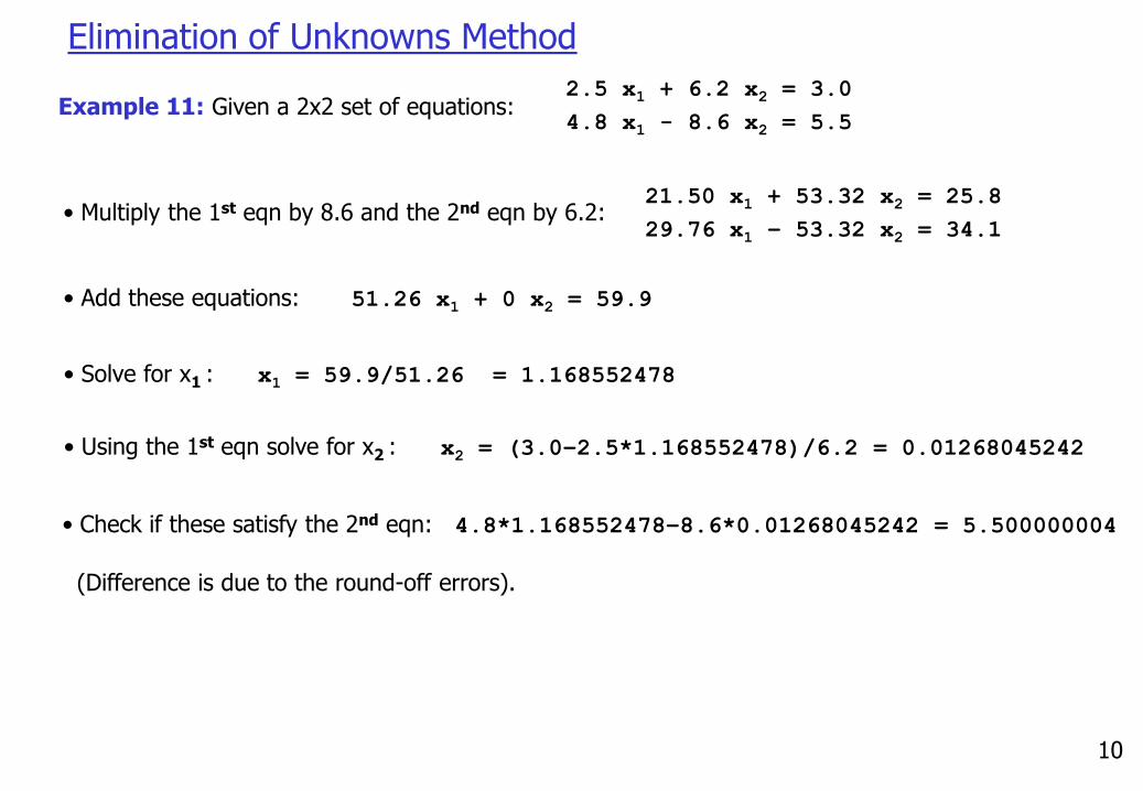
Example 11: Given a 2x2 set of equations:2.5 x1 + 6.2 x2 = 3.0

4.8 x1 - 8.6 x2 = 5.5

• Multiply the 1st eqn by 8.6 and the 2nd eqn by 6.2:21.50 x1 + 53.32 x2 = 25.8

29.76 x1 – 53.32 x2 = 34.1

• Add these equations: 51.26 x1 + 0 x2 = 59.9

• Solve for x1 : x1 = 59.9/51.26 = 1.168552478

• Using the 1st eqn solve for x2 : x2 = (3.0–2.5*1.168552478)/6.2 = 0.01268045242

• Check if these satisfy the 2nd eqn: 4.8*1.168552478–8.6*0.01268045242 = 5.500000004

(Difference is due to the round-off errors).

11

Naive Gauss Elimination Method

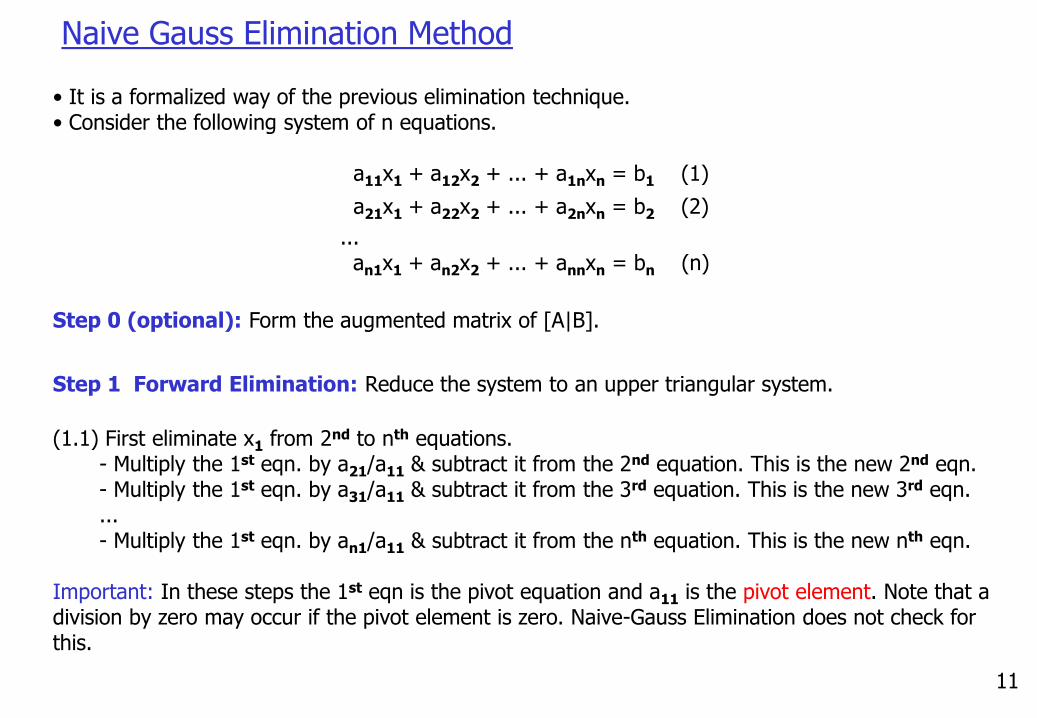
• It is a formalized way of the previous elimination technique.• Consider the following system of n equations.

a11x1 + a12x2 + ... + a1nxn = b1 (1)

a21x1 + a22x2 + ... + a2nxn = b2 (2)

...an1x1 + an2x2 + ... + annxn = bn (n)

Step 0 (optional): Form the augmented matrix of [A|B].

Step 1 Forward Elimination: Reduce the system to an upper triangular system.

(1.1) First eliminate x1 from 2nd to nth equations.- Multiply the 1st eqn. by a21/a11 & subtract it from the 2nd equation. This is the new 2nd eqn.- Multiply the 1st eqn. by a31/a11 & subtract it from the 3rd equation. This is the new 3rd eqn....- Multiply the 1st eqn. by an1/a11 & subtract it from the nth equation. This is the new nth eqn.

Important: In these steps the 1st eqn is the pivot equation and a11 is the pivot element. Note that a division by zero may occur if the pivot element is zero. Naive-Gauss Elimination does not check for this.

12

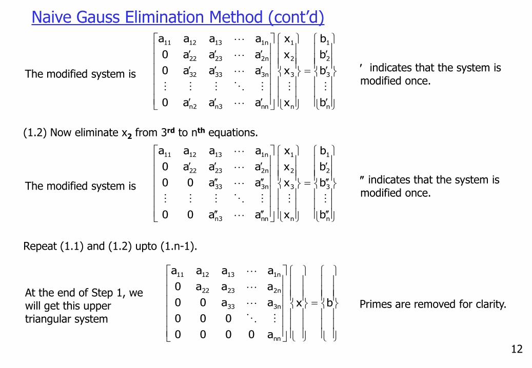
Naive Gauss Elimination Method (cont’d)

(1.2) Now eliminate x2 from 3rd to nth equations.

indicates that the system is modified once.

The modified system is

n

3

2

1

n

3

2

1

nn3n2n

n33332

n22322

n1131211

b

b

b

b

x

x

x

x

aaa0

aaa0

aaa0

aaaa

indicates that the system is modified once.

The modified system is

n

3

2

1

n

3

2

1

nn3n

n333

n22322

n1131211

b

b

b

b

x

x

x

x

aa00

aa00

aaa0

aaaa

Repeat (1.1) and (1.2) upto (1.n-1).

bx

a0000

000

aa00

aaa0

aaaa

nn

n333

n22322

n1131211

Primes are removed for clarity.At the end of Step 1, we will get this upper triangular system

13

Naive Gauss Elimination Method (cont’d)

Step 2 Back substitution: Find the unknowns starting from the last equation.

(2.1) Last equation involves only xn. Solve for it.(2.1) Use this xn in the (n-1)th equation and solve for xn-1....(2.n) Use all previously calculated x values in the 1st eqn and solve for x1.

Example 12: Solve the following system using Naive Gauss Elimination.

6x1 – 2x2 + 2x3 + 4x4 = 16

12x1 – 8x2 + 6x3 + 10x4 = 26

3x1 – 13x2 + 9x3 + 3x4 = -19

-6x1 + 4x2 + x3 - 18x4 = -34

Step 0: Form the augmented matrix

6 –2 2 4 | 16

12 –8 6 10 | 26

3 –13 9 3 | -19

-6 4 1 -18 | -34

14

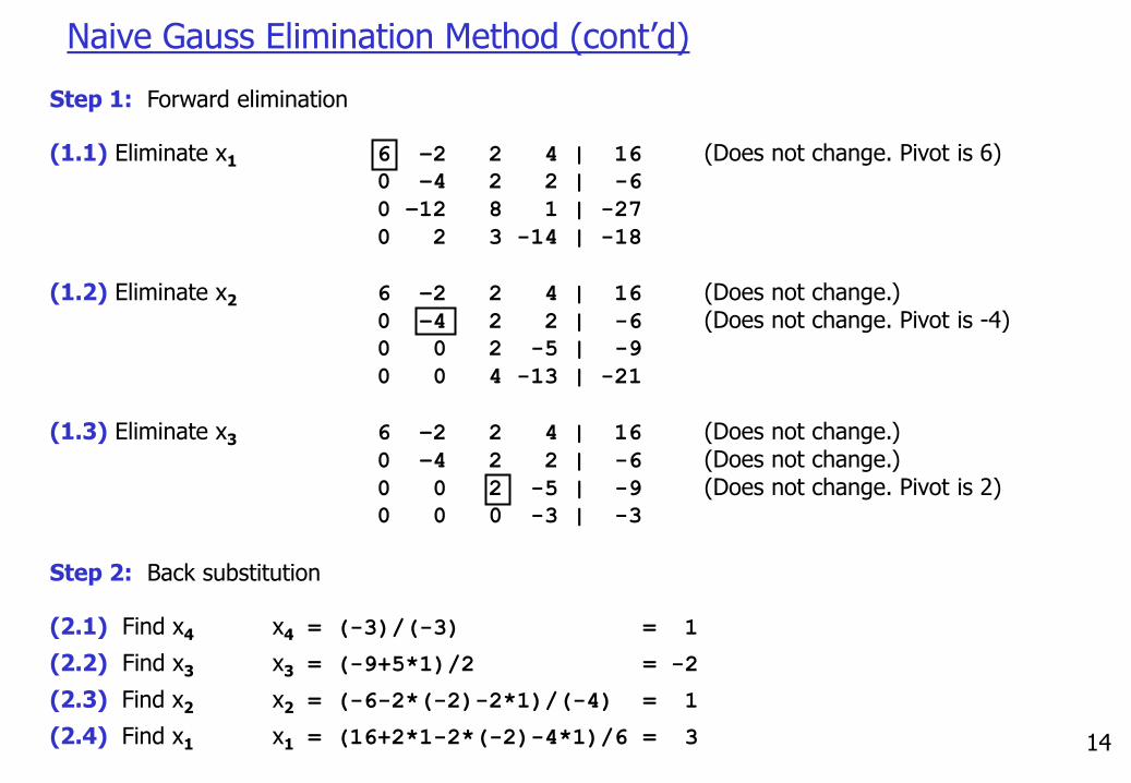
Naive Gauss Elimination Method (cont’d)

Step 1: Forward elimination

(1.1) Eliminate x1 6 –2 2 4 | 16 (Does not change. Pivot is 6)0 –4 2 2 | -6

0 –12 8 1 | -27

0 2 3 -14 | -18

(1.2) Eliminate x2 6 –2 2 4 | 16 (Does not change.)0 –4 2 2 | -6 (Does not change. Pivot is -4)0 0 2 -5 | -9

0 0 4 -13 | -21

(1.3) Eliminate x3 6 –2 2 4 | 16 (Does not change.)0 –4 2 2 | -6 (Does not change.)0 0 2 -5 | -9 (Does not change. Pivot is 2)0 0 0 -3 | -3

Step 2: Back substitution

(2.1) Find x4 x4 = (-3)/(-3) = 1

(2.2) Find x3 x3 = (-9+5*1)/2 = -2

(2.3) Find x2 x2 = (-6-2*(-2)-2*1)/(-4) = 1

(2.4) Find x1 x1 = (16+2*1-2*(-2)-4*1)/6 = 3

15

Pseudocode for the Naive Gauss Elimination Method

Forward Elimination

LOOP k from 1 to n-1

LOOP i from k+1 to n

FACTOR = A ik / A kk

LOOP j from k+1 to n

A ij = A ij – FACTOR * A kj

END LOOP

B i = B i – FACTOR * B k

ENDLOOP

ENDLOOP

Back Substitution

X n = B n / A nn

LOOP i from n-1 to 1

SUM = 0.0

LOOP j from i+1 to n

SUM = SUM + A ij * X j

END LOOP

X i = (B i – SUM) / A ii

ENDLOOP

For a general nxn system [A] {x} = {B}

Exercise 13: Implement this in C. Write a main program and two functions. You need to know how to pass matrices to the functions.

16

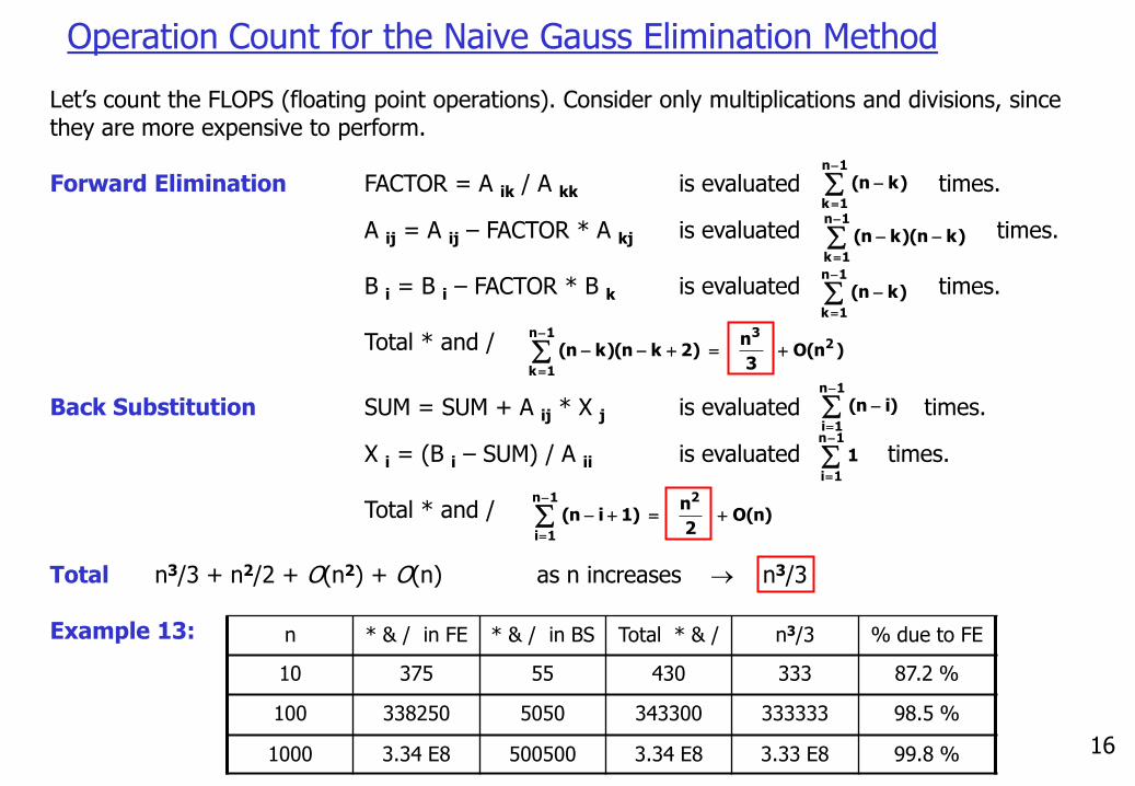
Let’s count the FLOPS (floating point operations). Consider only multiplications and divisions, since they are more expensive to perform.

Forward Elimination FACTOR = A ik / A kk is evaluated times.

A ij = A ij – FACTOR * A kj is evaluated times.

B i = B i – FACTOR * B k is evaluated times.

Total * and /

Back Substitution SUM = SUM + A ij * X j is evaluated times.

X i = (B i – SUM) / A ii is evaluated times.

Total * and /

Total n3/3 + n2/2 + O(n2) + O(n) as n increases n3/3

Example 13:

Operation Count for the Naive Gauss Elimination Method

1n

1k

)kn(

1n

1k

)kn)(kn(

1n

1k

)kn(

)n(O3

n)2kn()kn( 2

31n

1k

1n

1i

)in(

1n

1i

1

)n(O 2

n )1in(

21n

1i

n * & / in FE * & / in BS Total * & / n3/3 % due to FE

10 375 55 430 333 87.2 %

100 338250 5050 343300 333333 98.5 %

1000 3.34 E8 500500 3.34 E8 3.33 E8 99.8 %

17

• In Naive Gauss Elimination, a division by zero occurs if the pivot element is zero. Note that zero pivot elements may be created during the elimination step even if they are not present in the original matrix.

• Pivoting is used to avoid this problem. We interchange rows and columns at each step to put the coefficient with the largest magnitude on the diagonal.

• In addition to avoiding the division by zero problem, pivoting reduces the round-off errors. It makes the solution of ill-conditioned systems easier.

• Complete pivoting uses both row and column interchanges. It is not used frequently.

• Partial pivoting uses only row interchanges. We will use this.

• When there are large differences in magnitude of coefficients in one equation compared to the other equations we may also need scaling. Details will come later.

Pivoting

18

Pivoting Example

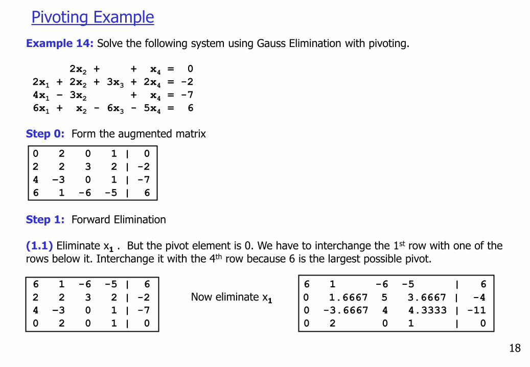
Example 14: Solve the following system using Gauss Elimination with pivoting.

2x2 + + x4 = 0

2x1 + 2x2 + 3x3 + 2x4 = -2

4x1 – 3x2 + x4 = -7

6x1 + x2 - 6x3 - 5x4 = 6

Step 0: Form the augmented matrix

0 2 0 1 | 0

2 2 3 2 | -2

4 –3 0 1 | -7

6 1 -6 -5 | 6

Step 1: Forward Elimination

(1.1) Eliminate x1 . But the pivot element is 0. We have to interchange the 1st row with one of the rows below it. Interchange it with the 4th row because 6 is the largest possible pivot.

6 1 -6 -5 | 6 6 1 -6 -5 | 6

2 2 3 2 | -2 Now eliminate x1 0 1.6667 5 3.6667 | -4

4 –3 0 1 | -7 0 -3.6667 4 4.3333 | -11

0 2 0 1 | 0 0 2 0 1 | 0

19

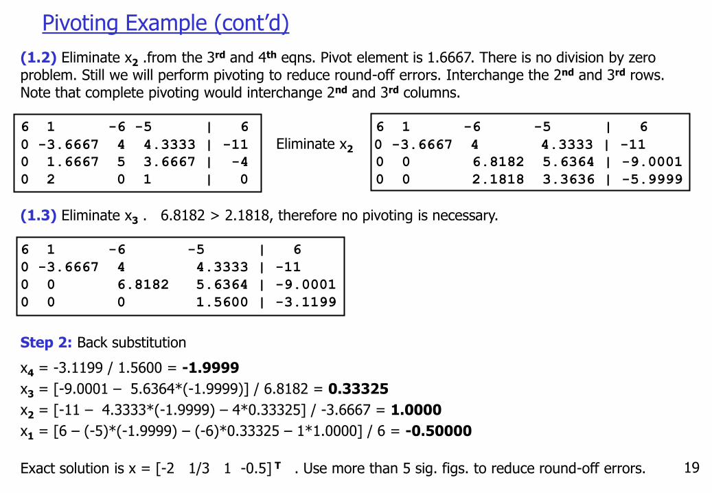
Pivoting Example (cont’d)

(1.2) Eliminate x2 .from the 3rd and 4th eqns. Pivot element is 1.6667. There is no division by zero problem. Still we will perform pivoting to reduce round-off errors. Interchange the 2nd and 3rd rows. Note that complete pivoting would interchange 2nd and 3rd columns.

6 1 -6 -5 | 6 6 1 -6 -5 | 6

0 -3.6667 4 4.3333 | -11 Eliminate x2 0 -3.6667 4 4.3333 | -11

0 1.6667 5 3.6667 | -4 0 0 6.8182 5.6364 | -9.0001

0 2 0 1 | 0 0 0 2.1818 3.3636 | -5.9999

(1.3) Eliminate x3 . 6.8182 > 2.1818, therefore no pivoting is necessary.

6 1 -6 -5 | 6

0 -3.6667 4 4.3333 | -11

0 0 6.8182 5.6364 | -9.0001

0 0 0 1.5600 | -3.1199

Step 2: Back substitution

x4 = -3.1199 / 1.5600 = -1.9999

x3 = [-9.0001 – 5.6364*(-1.9999)] / 6.8182 = 0.33325

x2 = [-11 – 4.3333*(-1.9999) – 4*0.33325] / -3.6667 = 1.0000

x1 = [6 – (-5)*(-1.9999) – (-6)*0.33325 – 1*1.0000] / 6 = -0.50000

Exact solution is x = [-2 1/3 1 -0.5] T . Use more than 5 sig. figs. to reduce round-off errors.

20

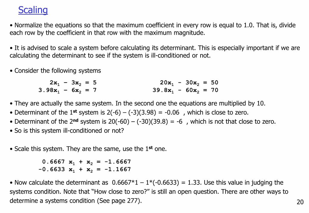
Scaling

• Normalize the equations so that the maximum coefficient in every row is equal to 1.0. That is, divide each row by the coefficient in that row with the maximum magnitude.

• It is advised to scale a system before calculating its determinant. This is especially important if we are calculating the determinant to see if the system is ill-conditioned or not.

• Consider the following systems

2x1 – 3x2 = 5 20x1 - 30x2 = 50

3.98x1 – 6x2 = 7 39.8x1 - 60x2 = 70

• They are actually the same system. In the second one the equations are multiplied by 10.

• Determinant of the 1st system is 2(-6) – (-3)(3.98) = -0.06 , which is close to zero.

• Determinant of the 2nd system is 20(-60) – (-30)(39.8) = -6 , which is not that close to zero.

• So is this system ill-conditioned or not?

• Scale this system. They are the same, use the 1st one.

0.6667 x1 + x2 = -1.6667

-0.6633 x1 + x2 = -1.1667

• Now calculate the determinant as 0.6667*1 – 1*(-0.6633) = 1.33. Use this value in judging the

systems condition. Note that “How close to zero?” is still an open question. There are other ways to

determine a systems condition (See page 277).

21

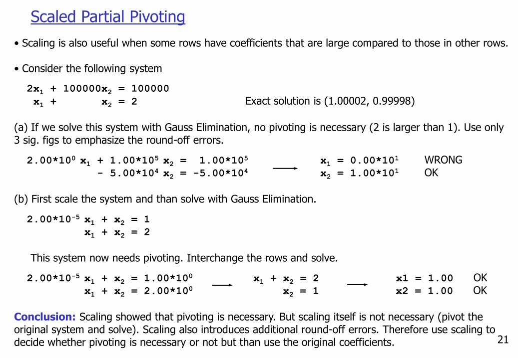
Scaled Partial Pivoting

• Scaling is also useful when some rows have coefficients that are large compared to those in other rows.

• Consider the following system

2x1 + 100000x2 = 100000

x1 + x2 = 2 Exact solution is (1.00002, 0.99998)

(a) If we solve this system with Gauss Elimination, no pivoting is necessary (2 is larger than 1). Use only 3 sig. figs to emphasize the round-off errors.

2.00*100 x1 + 1.00*105 x2 = 1.00*105 x1 = 0.00*101 WRONG- 5.00*104 x2 = -5.00*104 x2 = 1.00*101 OK

(b) First scale the system and than solve with Gauss Elimination.

2.00*10-5 x1 + x2 = 1

x1 + x2 = 2

This system now needs pivoting. Interchange the rows and solve.

2.00*10-5 x1 + x2 = 1.00*100 x1 + x2 = 2 x1 = 1.00 OKx1 + x2 = 2.00*100 x2 = 1 x2 = 1.00 OK

Conclusion: Scaling showed that pivoting is necessary. But scaling itself is not necessary (pivot the original system and solve). Scaling also introduces additional round-off errors. Therefore use scaling to decide whether pivoting is necessary or not but than use the original coefficients.

22

Example for Gauss Elimination with Scaled Partial Pivoting

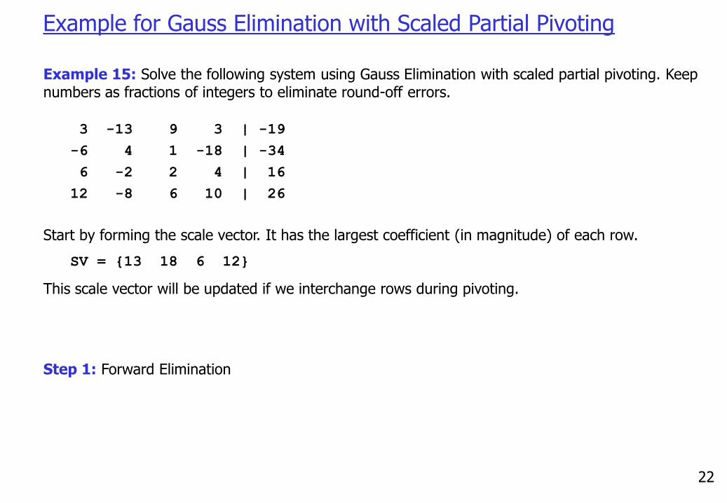
Example 15: Solve the following system using Gauss Elimination with scaled partial pivoting. Keep numbers as fractions of integers to eliminate round-off errors.

3 -13 9 3 | -19

-6 4 1 -18 | -34

6 -2 2 4 | 16

12 -8 6 10 | 26

Start by forming the scale vector. It has the largest coefficient (in magnitude) of each row.

SV = {13 18 6 12}

This scale vector will be updated if we interchange rows during pivoting.

Step 1: Forward Elimination

23

Example for Gauss Elimination with Scaled Pivoting (cont’d)

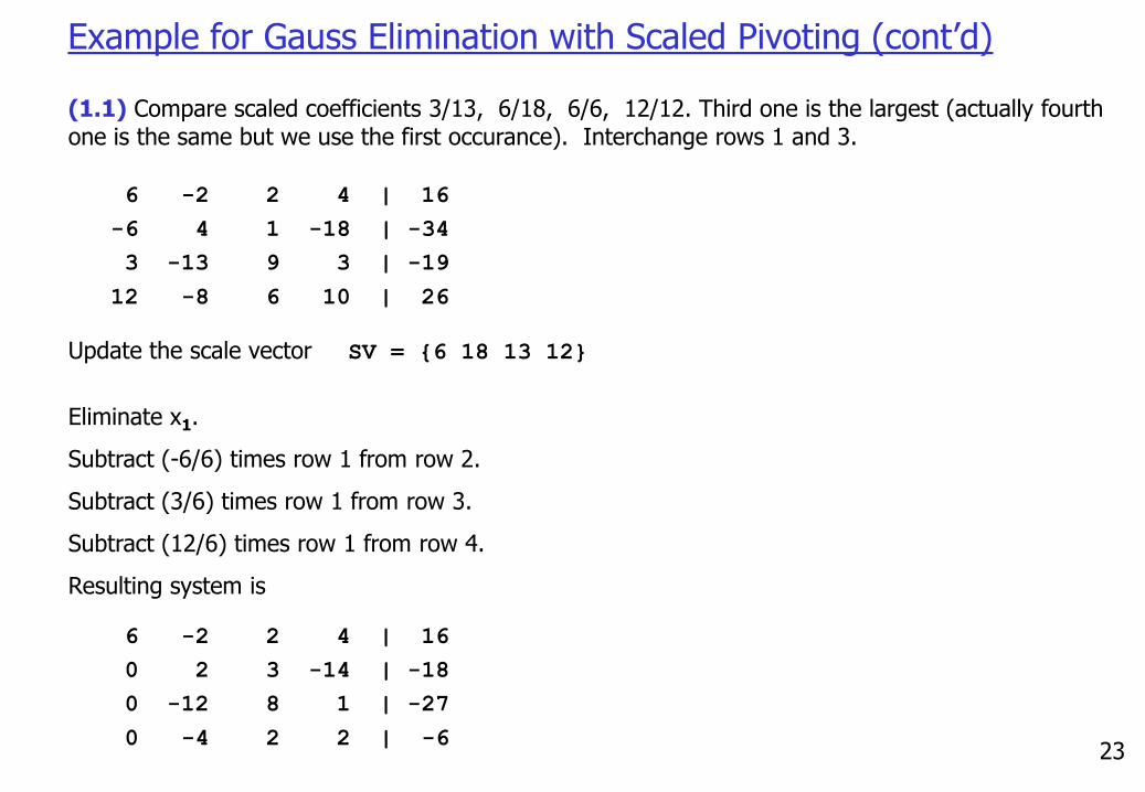
(1.1) Compare scaled coefficients 3/13, 6/18, 6/6, 12/12. Third one is the largest (actually fourth one is the same but we use the first occurance). Interchange rows 1 and 3.

6 -2 2 4 | 16

-6 4 1 -18 | -34

3 -13 9 3 | -19

12 -8 6 10 | 26

Update the scale vector SV = {6 18 13 12}

Eliminate x1.

Subtract (-6/6) times row 1 from row 2.

Subtract (3/6) times row 1 from row 3.

Subtract (12/6) times row 1 from row 4.

Resulting system is

6 -2 2 4 | 16

0 2 3 -14 | -18

0 -12 8 1 | -27

0 -4 2 2 | -6

24

Example for Gauss Elimination with Scaled Pivoting (cont’d)

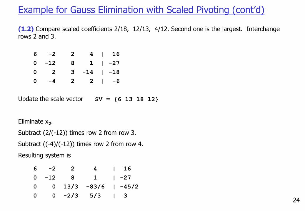
(1.2) Compare scaled coefficients 2/18, 12/13, 4/12. Second one is the largest. Interchange rows 2 and 3.

6 -2 2 4 | 16

0 -12 8 1 | -27

0 2 3 -14 | -18

0 -4 2 2 | -6

Update the scale vector SV = {6 13 18 12}

Eliminate x2.

Subtract (2/(-12)) times row 2 from row 3.

Subtract ((-4)/(-12)) times row 2 from row 4.

Resulting system is

6 -2 2 4 | 16

0 -12 8 1 | -27

0 0 13/3 -83/6 | -45/2

0 0 -2/3 5/3 | 3

25

Example for Gauss Elimination with Scaled Pivoting (cont’d)

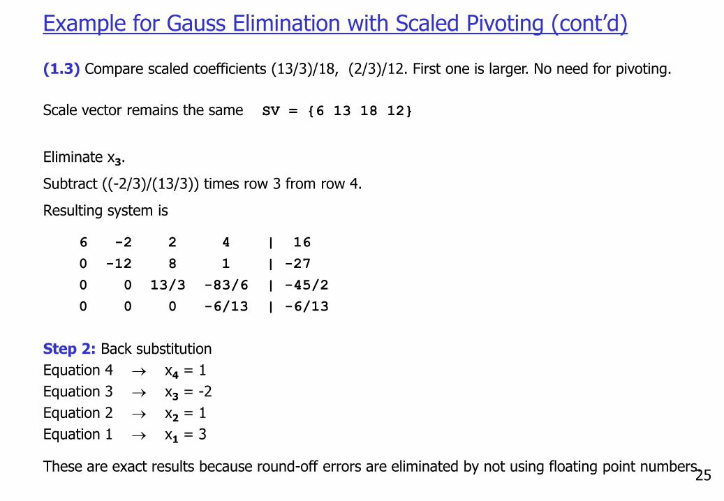
(1.3) Compare scaled coefficients (13/3)/18, (2/3)/12. First one is larger. No need for pivoting.

Scale vector remains the same SV = {6 13 18 12}

Eliminate x3.

Subtract ((-2/3)/(13/3)) times row 3 from row 4.

Resulting system is

6 -2 2 4 | 16

0 -12 8 1 | -27

0 0 13/3 -83/6 | -45/2

0 0 0 -6/13 | -6/13

Step 2: Back substitution

Equation 4 x4 = 1

Equation 3 x3 = -2

Equation 2 x2 = 1

Equation 1 x1 = 3

These are exact results because round-off errors are eliminated by not using floating point numbers.

26

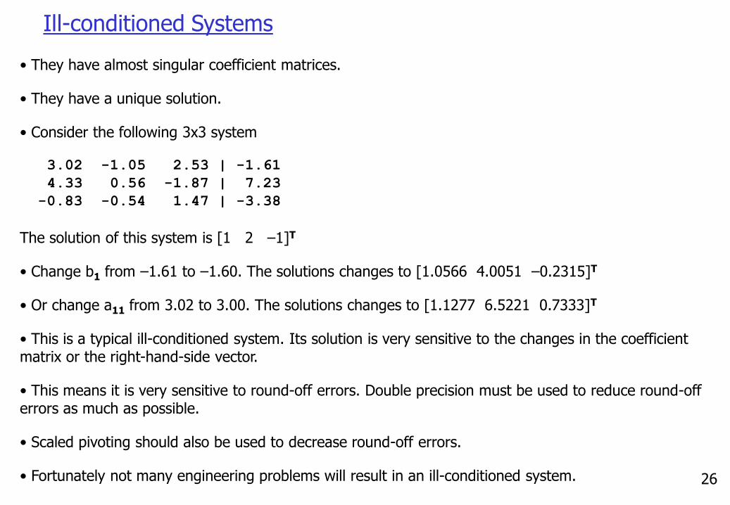
Ill-conditioned Systems

• They have almost singular coefficient matrices.

• They have a unique solution.

• Consider the following 3x3 system

3.02 -1.05 2.53 | -1.61

4.33 0.56 -1.87 | 7.23

-0.83 -0.54 1.47 | -3.38

The solution of this system is [1 2 –1]T

• Change b1 from –1.61 to –1.60. The solutions changes to [1.0566 4.0051 –0.2315]T

• Or change a11 from 3.02 to 3.00. The solutions changes to [1.1277 6.5221 0.7333]T

• This is a typical ill-conditioned system. Its solution is very sensitive to the changes in the coefficient matrix or the right-hand-side vector.

• This means it is very sensitive to round-off errors. Double precision must be used to reduce round-off errors as much as possible.

• Scaled pivoting should also be used to decrease round-off errors.

• Fortunately not many engineering problems will result in an ill-conditioned system.

27

Other Uses of Gauss Elimination

• Gives the LU decomposition of A such that [L][U]=[A]. LU decomposition is useful if we are solving many systems with the same coefficient matrix A but different right-hand-side vectors (See page 266).

• It can be used to calculate the determinant of a matrix. At the end of the Forward Elimination step we get an upper triangular matrix. For this matrix the determinant is just the multiplication of diagonal elements. If we interchanged rows m times, than the deteminant can be calculated as

|A| = (-1)m * a11 * a22 * … ann

Example 16: Remember the example we used to describe pivoting. The A matrix was

0 2 0 1

2 2 3 2

4 –3 0 1

6 1 -6 -5

After the Forward Elimination step we found the following upper triangular matrix.

6 1 -6 -5

0 -3.6667 4 4.3333

0 0 6.8182 5.6364

0 0 0 1.5600

To get this, we used pivoting and interchanged rows twice. Therefore the determinant of A is

|A| = (-1)2 * 6 * (-3.6667) * 6.8182 * 1.56 = -234.0028

28

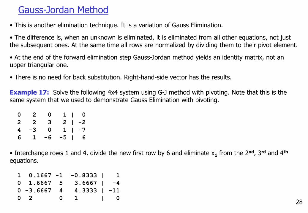
Gauss-Jordan Method

• This is another elimination technique. It is a variation of Gauss Elimination.

• The difference is, when an unknown is eliminated, it is eliminated from all other equations, not just the subsequent ones. At the same time all rows are normalized by dividing them to their pivot element.

• At the end of the forward elimination step Gauss-Jordan method yields an identity matrix, not an upper triangular one.

• There is no need for back substitution. Right-hand-side vector has the results.

Example 17: Solve the following 4x4 system using G-J method with pivoting. Note that this is the same system that we used to demonstrate Gauss Elimination with pivoting.

0 2 0 1 | 0

2 2 3 2 | -2

4 –3 0 1 | -7

6 1 -6 -5 | 6

• Interchange rows 1 and 4, divide the new first row by 6 and eliminate x1 from the 2nd, 3rd and 4th

equations.

1 0.1667 -1 -0.8333 | 1

0 1.6667 5 3.6667 | -4

0 -3.6667 4 4.3333 | -11

0 2 0 1 | 0

29

Gauss-Jordan Method (cont’d)

• Interchange rows 2 and 3, divide the new second row by -3.6667 and eliminate x2 from the 1st, 3rd

and 4th equations.

1 0 -0.8182 -0.6364 | 0.5

0 1 -1.0909 -1.1818 | 3

0 0 6.8182 5.6364 | -9

0 0 2.1818 3.3636 | -6

• No pivoting is required. Divide the third row by 6.8182 and eliminate x3 from the 1st, 2nd and 4th

equations.

1 0 0 0.04 | 0.58

0 1 0 -0.280 | 1.56

0 0 1 0 | -1.32

0 0 0 1.5599 | -3.12

• Divide the last row by 1.5599 and eliminate x4 from the 1st, 2nd and 3rd equations.

1 0 0 0 | -0.5

0 1 0 0 | 1.0001

0 0 1 0 | 0.3333

0 0 0 1 | -2

• Right-hand-side vector is the solution. No back substitution is required.

• Gauss-Jordan requires almost 50% more operations than Gauss Elimination (n3/2 instead of n3/3).

30

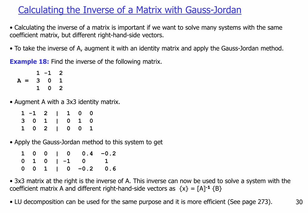
Calculating the Inverse of a Matrix with Gauss-Jordan

• Calculating the inverse of a matrix is important if we want to solve many systems with the same coefficient matrix, but different right-hand-side vectors.

• To take the inverse of A, augment it with an identity matrix and apply the Gauss-Jordan method.

Example 18: Find the inverse of the following matrix.

1 -1 2

A = 3 0 1

1 0 2

• Augment A with a 3x3 identity matrix.

1 -1 2 | 1 0 0

3 0 1 | 0 1 0

1 0 2 | 0 0 1

• Apply the Gauss-Jordan method to this system to get

1 0 0 | 0 0.4 –0.2

0 1 0 | -1 0 1

0 0 1 | 0 –0.2 0.6

• 3x3 matrix at the right is the inverse of A. This inverse can now be used to solve a system with the coefficient matrix A and different right-hand-side vectors as {x} = [A]-1 {B}

• LU decomposition can be used for the same purpose and it is more efficient (See page 273).

31

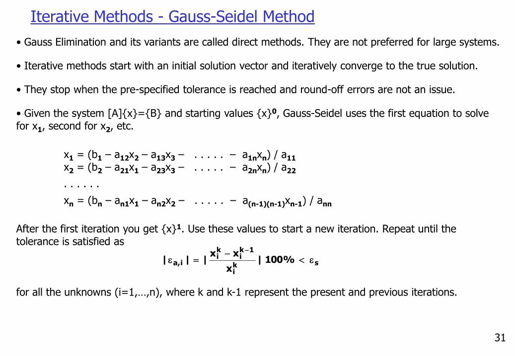
Iterative Methods - Gauss-Seidel Method

• Gauss Elimination and its variants are called direct methods. They are not preferred for large systems.

• Iterative methods start with an initial solution vector and iteratively converge to the true solution.

• They stop when the pre-specified tolerance is reached and round-off errors are not an issue.

• Given the system [A]{x}={B} and starting values {x}0, Gauss-Seidel uses the first equation to solve for x1, second for x2, etc.

x1 = (b1 – a12x2 – a13x3 – . . . . . – a1nxn) / a11

x2 = (b2 – a21x1 – a23x3 – . . . . . – a2nxn) / a22

. . . . . .

xn = (bn – an1x1 – an2x2 – . . . . . – a(n-1)(n-1)xn-1) / ann

After the first iteration you get {x}1. Use these values to start a new iteration. Repeat until the tolerance is satisfied as

for all the unknowns (i=1,…,n), where k and k-1 represent the present and previous iterations.

ski

1ki

ki

i,a %100 |x

xx| ||

32

Gauss-Seidel Example

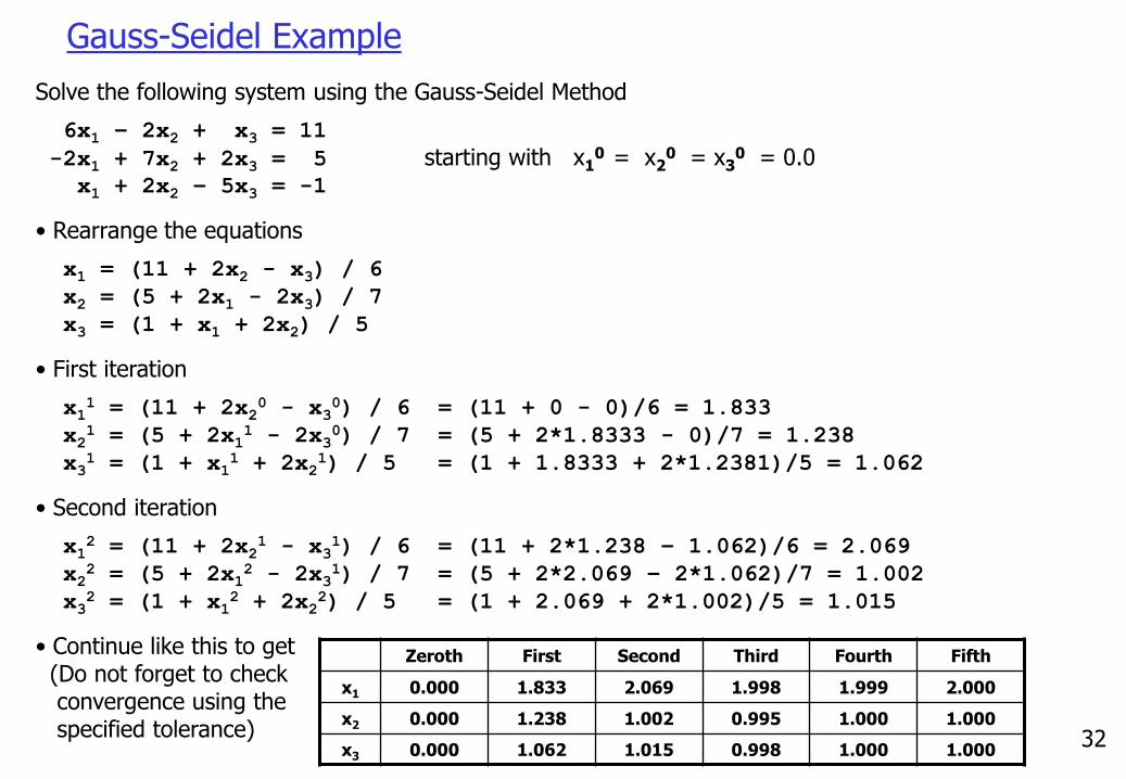
Solve the following system using the Gauss-Seidel Method

6x1 – 2x2 + x3 = 11

-2x1 + 7x2 + 2x3 = 5 starting with x10 = x2

0 = x30 = 0.0

x1 + 2x2 – 5x3 = -1

• Rearrange the equations

x1 = (11 + 2x2 - x3) / 6

x2 = (5 + 2x1 - 2x3) / 7

x3 = (1 + x1 + 2x2) / 5

• First iteration

x11 = (11 + 2x2

0 - x30) / 6 = (11 + 0 - 0)/6 = 1.833

x21 = (5 + 2x1

1 - 2x30) / 7 = (5 + 2*1.8333 - 0)/7 = 1.238

x31 = (1 + x1

1 + 2x21) / 5 = (1 + 1.8333 + 2*1.2381)/5 = 1.062

• Second iteration

x12 = (11 + 2x2

1 - x31) / 6 = (11 + 2*1.238 – 1.062)/6 = 2.069

x22 = (5 + 2x1

2 - 2x31) / 7 = (5 + 2*2.069 – 2*1.062)/7 = 1.002

x32 = (1 + x1

2 + 2x22) / 5 = (1 + 2.069 + 2*1.002)/5 = 1.015

• Continue like this to get (Do not forget to checkconvergence using thespecified tolerance)

Zeroth First Second Third Fourth Fifth

x1 0.000 1.833 2.069 1.998 1.999 2.000

x2 0.000 1.238 1.002 0.995 1.000 1.000

x3 0.000 1.062 1.015 0.998 1.000 1.000

33

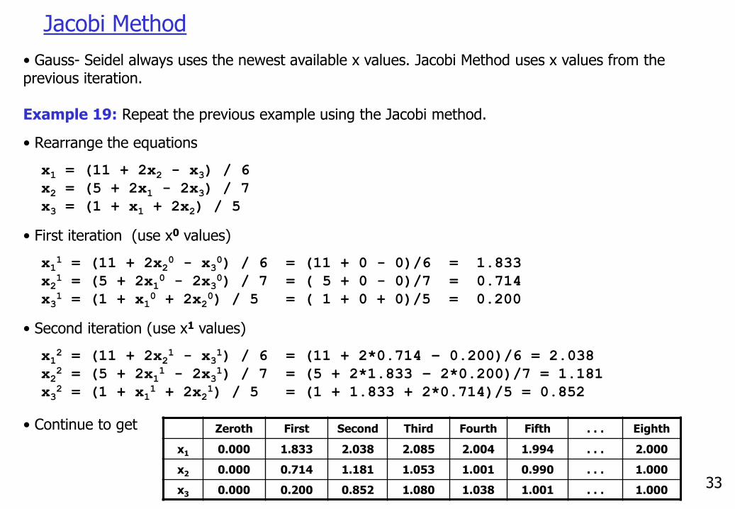
Jacobi Method

• Gauss- Seidel always uses the newest available x values. Jacobi Method uses x values from the previous iteration.

Example 19: Repeat the previous example using the Jacobi method.

• Rearrange the equations

x1 = (11 + 2x2 - x3) / 6

x2 = (5 + 2x1 - 2x3) / 7

x3 = (1 + x1 + 2x2) / 5

• First iteration (use x0 values)

x11 = (11 + 2x2

0 - x30) / 6 = (11 + 0 - 0)/6 = 1.833

x21 = (5 + 2x1

0 - 2x30) / 7 = ( 5 + 0 - 0)/7 = 0.714

x31 = (1 + x1

0 + 2x20) / 5 = ( 1 + 0 + 0)/5 = 0.200

• Second iteration (use x1 values)

x12 = (11 + 2x2

1 - x31) / 6 = (11 + 2*0.714 – 0.200)/6 = 2.038

x22 = (5 + 2x1

1 - 2x31) / 7 = (5 + 2*1.833 – 2*0.200)/7 = 1.181

x32 = (1 + x1

1 + 2x21) / 5 = (1 + 1.833 + 2*0.714)/5 = 0.852

• Continue to get Zeroth First Second Third Fourth Fifth . . . Eighth

x1 0.000 1.833 2.038 2.085 2.004 1.994 . . . 2.000

x2 0.000 0.714 1.181 1.053 1.001 0.990 . . . 1.000

x3 0.000 0.200 0.852 1.080 1.038 1.001 . . . 1.000

34

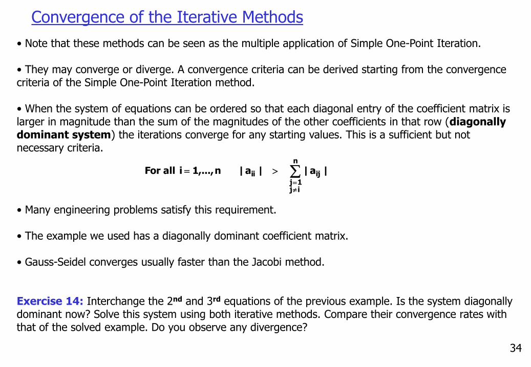
Convergence of the Iterative Methods

• Note that these methods can be seen as the multiple application of Simple One-Point Iteration.

• They may converge or diverge. A convergence criteria can be derived starting from the convergence criteria of the Simple One-Point Iteration method.

• When the system of equations can be ordered so that each diagonal entry of the coefficient matrix is larger in magnitude than the sum of the magnitudes of the other coefficients in that row (diagonally dominant system) the iterations converge for any starting values. This is a sufficient but not necessary criteria.

• Many engineering problems satisfy this requirement.

• The example we used has a diagonally dominant coefficient matrix.

• Gauss-Seidel converges usually faster than the Jacobi method.

Exercise 14: Interchange the 2nd and 3rd equations of the previous example. Is the system diagonally dominant now? Solve this system using both iterative methods. Compare their convergence rates with that of the solved example. Do you observe any divergence?

n

ij1j

ijii |a| |a| n1,..., i allFor

35

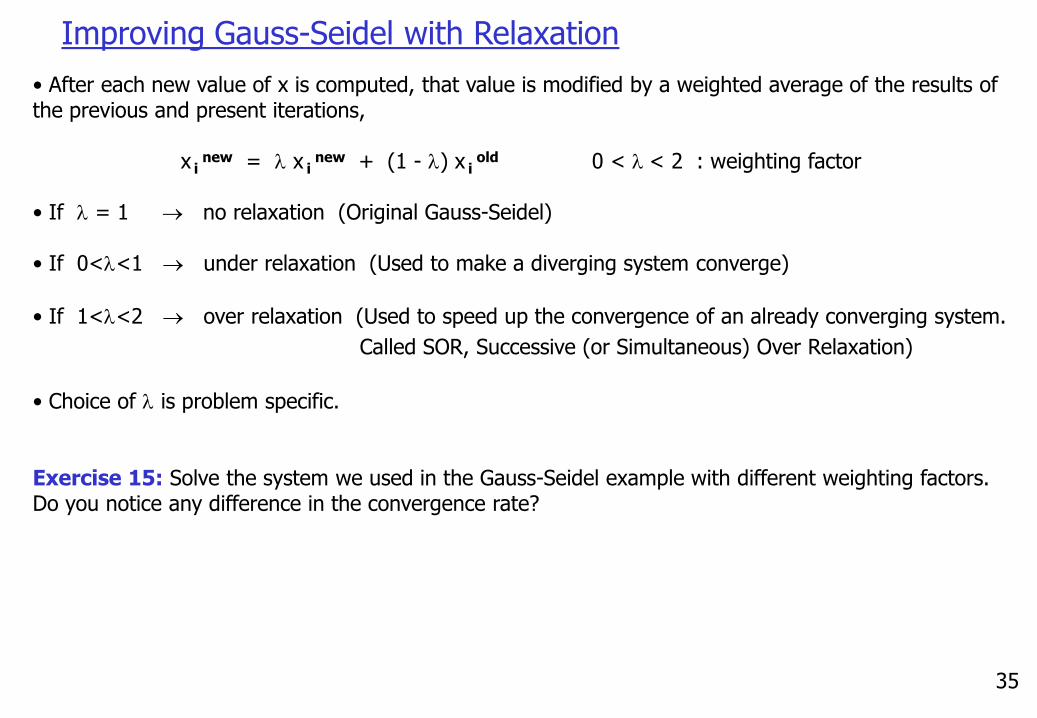
Improving Gauss-Seidel with Relaxation

• After each new value of x is computed, that value is modified by a weighted average of the results of the previous and present iterations,

x i new = l x i

new + (1 - l) x i old 0 < l < 2 : weighting factor

• If l = 1 no relaxation (Original Gauss-Seidel)

• If 0<l<1 under relaxation (Used to make a diverging system converge)

• If 1<l<2 over relaxation (Used to speed up the convergence of an already converging system.

Called SOR, Successive (or Simultaneous) Over Relaxation)

• Choice of l is problem specific.

Exercise 15: Solve the system we used in the Gauss-Seidel example with different weighting factors. Do you notice any difference in the convergence rate?

36

Pseudocode for the Gauss-Seidel Method

LOOP k from 1 to maxIter

LOOP i from 1 to n

x i = B i

LOOP j from 1 to n

IF (i j) x i = x i - A ij x j

ENDLOOP

x i = x i / A ii

ENDLOOP

CONVERGED = TRUE

LOOP i from 1 to n

OUTPUT x i

a = | (x i – x iold) / x i | * 100

IF (a > tolerance) CONVERGED = FALSE

ENDLOOP

IF (CONVERGED = TRUE) STOP

ENDLOOP

Exercise 16: Improve this pseudocode with relaxation.

Exercise 17: Modify this pseudocode for the Jacobi method.

37

Solving System of Nonlinear Equations

Example 20: Solving a 2x2 System Using Simple One-Point Iteration

Solve the following system of equations1ye

4yx

x

22

x

y

22

1

x4)x(gy

)y1ln()y(gx

Put the functions into the form x=g1(x,y), y=g2(x,y)

Select a starting values for x and y, such as x0=0.0 and y0=0.0. They don’t need to satisfy the equations. Use these values in g functions to calculate new values.

x1= g1(y0) = 0 y1= g2(x1) = -2

x2= g1(y1) = 1.098612289 y2= g2(x2) = -1.67124236

x3= g1(y2) = 0.982543669 y3= g2(x3) = -1.74201261

x4= g1(y3) = 1.00869218 y4= g2(x4) = -1.72700321

The solution is converging to the exact solution of x=1.004169 , y=-1.729637

Exercise 18: Solve the same system but rearrange the equations as x=ln(1-y) y = (4-x2)/y and start from x0=1 y0=-1.7. Remember that this method may diverge.

38

Solving System of Nonlinear Equations (cont’d)

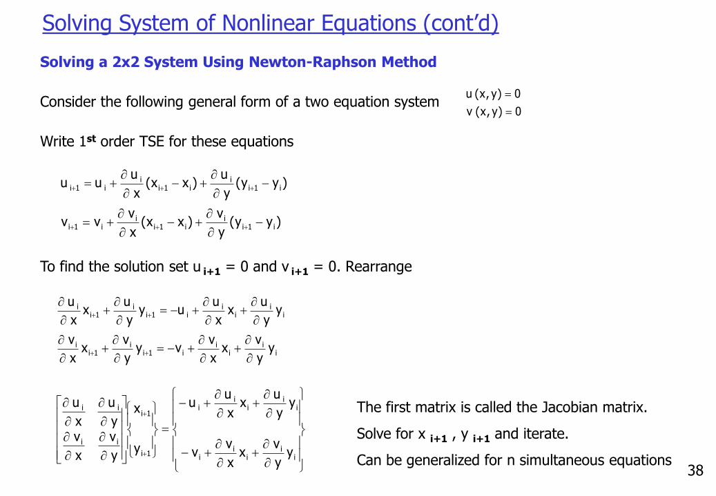
Solving a 2x2 System Using Newton-Raphson Method

Consider the following general form of a two equation system

Write 1st order TSE for these equations

0)y,x( v

0)y,x( u

)yy(y

v )xx(

x

v vv

)yy(y

u )xx(

x

u uu

i1ii

i1ii

i1i

i1ii

i1ii

i 1i

To find the solution set u i+1 = 0 and v i+1 = 0. Rearrange

ii

ii

i1ii

1ii

ii

ii

i 1ii

1ii

yy

vx

x

vvy

y

vx

x

v

yy

u x

x

u uy

y

u x

x

u

ii

ii

i

ii

ii

i

1i

1i

ii

i i

yy

vx

x

vv

yy

u x

x

u u

y

x

y

v

x

vy

u

x

u The first matrix is called the Jacobian matrix.

Solve for x i+1 , y i+1 and iterate.

Can be generalized for n simultaneous equations

39

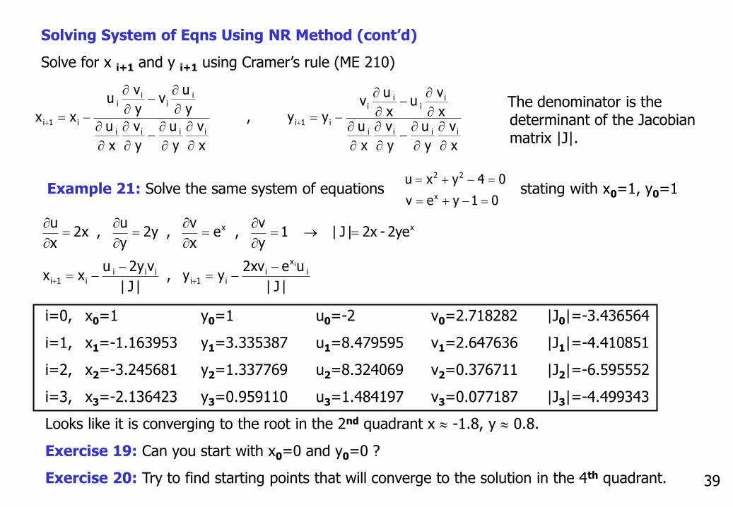
Solving System of Eqns Using NR Method (cont’d)

Solve for x i+1 and y i+1 using Cramer’s rule (ME 210)

x

v

y

u

y

v

x

u x

vu

x

u v

y y,

x

v

y

u

y

v

x

u

y

u v

y

v u

xxii ii

ii

i i

i1iii ii

i i

ii

i1i

The denominator is the determinant of the Jacobian matrix |J|.

Example 21: Solve the same system of equations stating with x0=1, y0=101yev

04yxux

22

i=0, x0=1 y0=1 u0=-2 v0=2.718282 |J0|=-3.436564

i=1, x1=-1.163953 y1=3.335387 u1=8.479595 v1=2.647636 |J1|=-4.410851

i=2, x2=-3.245681 y2=1.337769 u2=8.324069 v2=0.376711 |J2|=-6.595552

i=3, x3=-2.136423 y3=0.959110 u3=1.484197 v3=0.077187 |J3|=-4.499343

Looks like it is converging to the root in the 2nd quadrant x -1.8, y 0.8.

Exercise 19: Can you start with x0=0 and y0=0 ?

Exercise 20: Try to find starting points that will converge to the solution in the 4th quadrant.

|J|

uexv2y y,

|J|

vy2uxx

2ye-2x|J| 1y

v , e

x

v , y2

y

u , x2

x

u

i

x

ii1i

iii i1i

xx

i

40

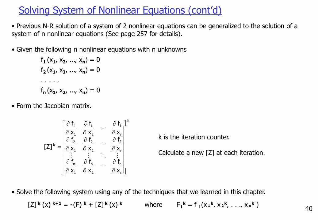
Solving System of Nonlinear Equations (cont’d)

• Previous N-R solution of a system of 2 nonlinear equations can be generalized to the solution of a system of n nonlinear equations (See page 257 for details).

• Given the following n nonlinear equations with n unknowns

f1 (x1, x2, ..., xn) = 0

f2 (x1, x2, ..., xn) = 0

. . . . .

fn (x1, x2, ..., xn) = 0

• Form the Jacobian matrix.

k is the iteration counter.

Calculate a new [Z] at each iteration.

• Solve the following system using any of the techniques that we learned in this chapter.

[Z] k {x} k+1 = -{F} k + [Z] k {x} k where F ik = f i (x 1

k, x 2k, . . ., x n

k )

k

n

n

2

n

1

n

n

2

2

2

1

2

n

1

2

1

1

1

k

x

f

x

f

x

f

x

f

x

f

x

f x

f

x

f

x

f

]Z[

41

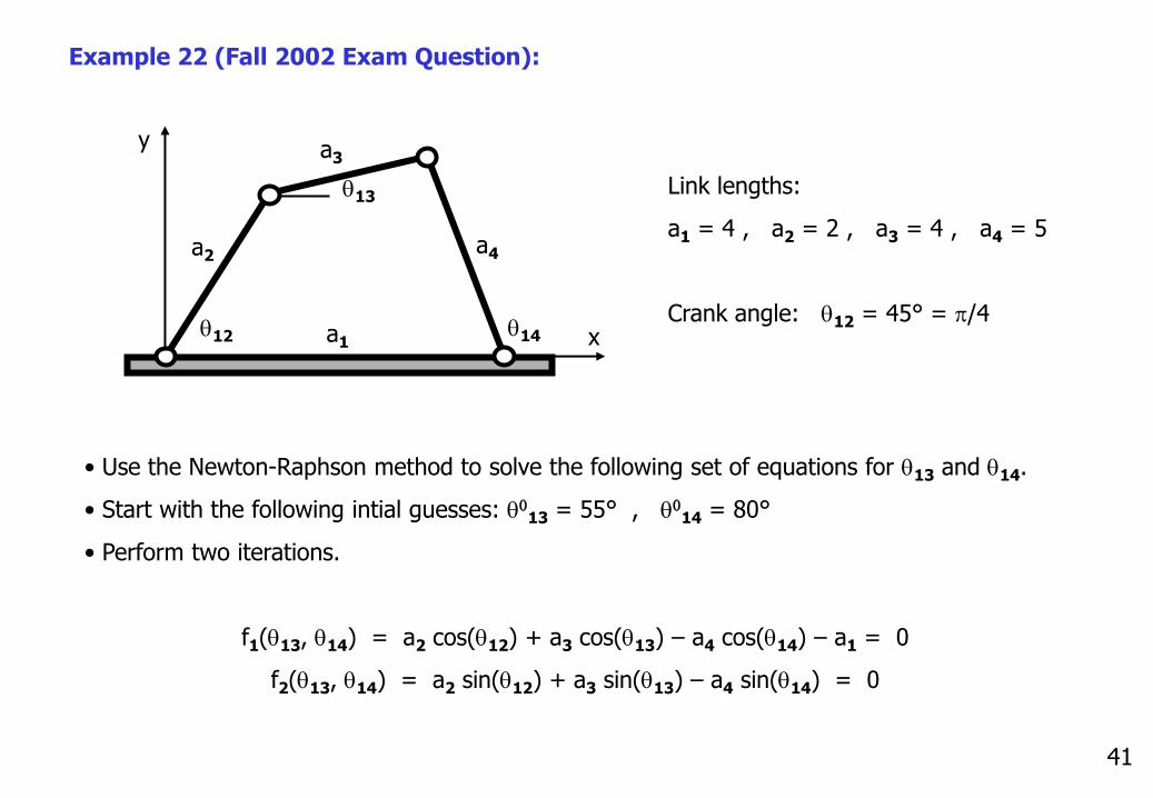
Example 22 (Fall 2002 Exam Question):

x

y

a2

a3

a4

a1q12

q13

q14

Link lengths:

a1 = 4 , a2 = 2 , a3 = 4 , a4 = 5

Crank angle: q12 = 45° = p/4

• Use the Newton-Raphson method to solve the following set of equations for q13 and q14.

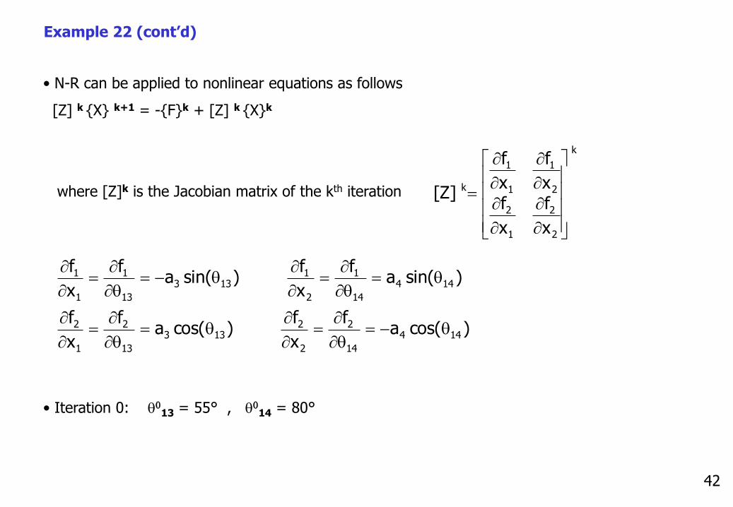
• Start with the following intial guesses: q013 = 55° , q014 = 80°

• Perform two iterations.

f1(q13, q14) = a2 cos(q12) + a3 cos(q13) – a4 cos(q14) – a1 = 0

f2(q13, q14) = a2 sin(q12) + a3 sin(q13) – a4 sin(q14) = 0

42

• N-R can be applied to nonlinear equations as follows

[Z] k {X} k+1 = -{F}k + [Z] k {X}k

where [Z]k is the Jacobian matrix of the kth iteration

• Iteration 0: q013 = 55° , q014 = 80°

k

2

2

1

2

2

1

1

1

k

x

f

x

fx

f

x

f

]Z[

)cos(af

x

f )cos(a

f

x

f

)sin(af

x

f )sin(a

f

x

f

144

14

2

2

2133

13

2

1

2

144

14

1

2

1133

13

1

1

1

qq

q

q

qq

q

q

Example 22 (cont’d)

43

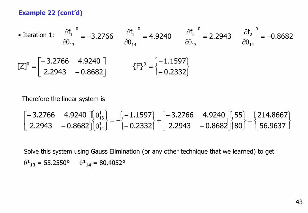
• Iteration 1:

Therefore the linear system is

Solve this system using Gauss Elimination (or any other technique that we learned) to get

q113 = 55.2550° q1

14 = 80.4052°

2332.0

1597.1}{F

8682.02943.2

9240.42766.3]Z[ 00

q

q

9637.56

8667.214

80

55

8682.02943.2

9240.42766.3

2332.0

1597.1

8682.02943.2

9240.42766.3114

113

8682.0f

2943.2f

9240.4f

2766.3f

0

14

2

0

13

2

0

14

1

0

13

1 q

q

q

q

Example 22 (cont’d)

44

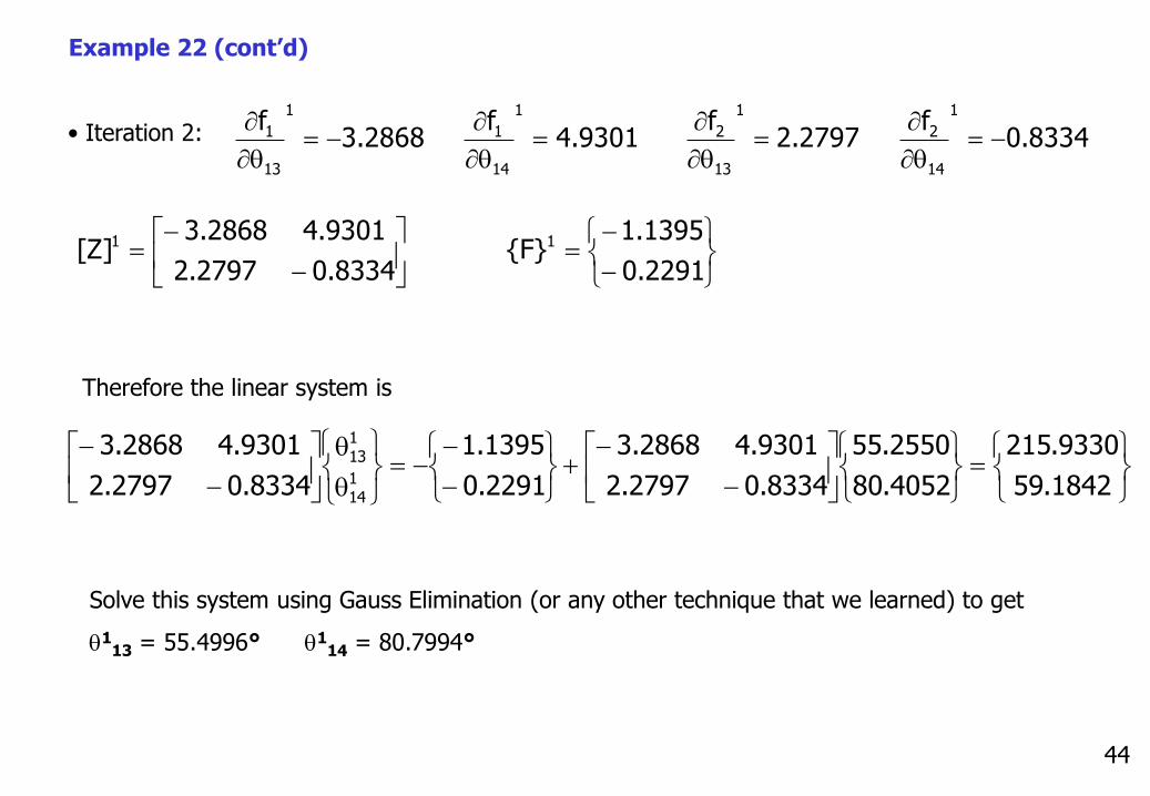
• Iteration 2:

Therefore the linear system is

Solve this system using Gauss Elimination (or any other technique that we learned) to get

q113 = 55.4996° q1

14 = 80.7994°

2291.0

1395.1}{F

8334.02797.2

9301.42868.3]Z[ 11

q

q

1842.59

9330.215

4052.80

2550.55

8334.02797.2

9301.42868.3

2291.0

1395.1

8334.02797.2

9301.42868.3114

113

8334.0f

2797.2f

9301.4f

2868.3f

1

14

2

1

13

2

1

14

1

1

13

1 q

q

q

q

Example 22 (cont’d)