MCLECTURE1.PPT

7/27/2019 MCLECTURE1.PPT

http://slidepdf.com/reader/full/mclecture1ppt 1/36

10/30/2013 (C) 2001, Ernest L. Hall, University of Cincinnati 1

ManufacturingControls

FALL 2001




Manufacturing Controls

20-IND-475-001

TIME: 11:00--12:15 PM, Tuesday and Thursday;Room: 617 ERC

INSTRUCTOR: Professor Ernest L. Hall, P.E. GeierProfessor of Robotics

PHONE: 556-2730, Email: [email protected] OFFICE HOURS: 1:00--2:00 and 3:30--4:30 PM,

TH, 681 or 508 Rhodes

WWW: http://www.eng.uc.edu/~elhall/mc.html

TEXT: Devdas Shetty and Richard A. Kolk,Mechatronics System Design, PWS Publishing,Boston.

NOTES: www.robotics.uc.edu/MC2001/

mailto:[email protected]

mailto:[email protected]




Course objective

To provide a broad basis for understanding

modern digital control theory for

manufacturing

with enough detailed examples to provide

practical experience in understanding stability

and tuning of digital motion controllers using

modern design tools such as Matlab.




Syllabus

DATE TOPIC NOTES 1. Sep. 20 Mechatronics Design Process Ch. 1

2. Sep. 25 System Modeling and Simulation Ch. 2

3. Sep. 27 Laplace Transforms and Transfer Functions Ch. 2

4. Oct. 2 Electrical Examples Ch.2, Notes 5. Oct. 4 Mechanical Examples Ch.2, Notes

6. Oct. 9 Thermal and Fluid Examples, QUIZ 1 (Take Home)

7. Oct. 11 Sensors and Transducers Ch. 3

8. Oct. 16 Advanced MATLAB

9. Oct. 18 Analog and Digital Sensing Ch. 3,

Notes 10. Oct. 23 Actuating Devices Ch. 4

11. Oct. 25 DC Motor Model Ch. 4,Notes

12. Oct. 30 Boolean Logic Ch. 5

13. Nov. 1 Programmable Logic Controllers Ch. 5, Notes

14. Nov. 6 Stability and Compensators, P, PI and PD Ch. 6

15. Nov. 8 PID Controllers Ch. 7

16. Nov. 13 QUIZ 2 (In Class - Open Book)

17. Nov. 15 Practical and Optimal Compensator Design Ch. 8 18. Nov. 20 Frequency Response Methods Ch. 9, Notes

19. Nov. 22 THANKSGIVING HOLIDAY Ch. 9, Notes

20. Nov. 27 Optimal Design of a Motion Control System Ch. 9, Notes

21. Nov. 29 QUIZ 3 (In Class - Closed Book)

22. Dec. FINAL EXAM (In Class - Closed Book) Comprehensive




Grading System

FG = .2(Q1 + Q2 + Q3 + F + HW)

Where

FG = Final grade Qi = Quiz i

F = Final exam

HW = Homework.




Note to Students:

You are expected to attend class, read the

text, and use the computer. Computer

accounts and Email are required. You will

find MATLAB essential for some of the

homework. The syllabus topics are guidelines

and may be adapted as required to improve

your understanding during the quarter.




Today’s objective

To provide an introduction to systems theory

and the use of Matlab by studying a simple

example, the flexible link pendulum.




Plant

System

Human – not yet fully

understood

Machine – Linear and

non-linear systemstheory

Man-Machine – Best of

both

Has both input and

output - normally




Architecture of System

Uncontrollable

Example - sun

Plant




Architecture of System

Unobservable

Example – black hole

Plant




Non-servo system

Plant

connection

(b) Non-servo system




Feedback Control

Feedback system – measurements

compared to input and error used to drive

plant

Plant

connection

Sensors




Digital Motion Control

Motion control is one of thetechnological foundations ofindustrial automation.

motion of a product

path of a cutting tool motion of an industrial robot

arm conducting seamwelding

motion of a parcel beingmoved from a storage bin toa loading dock by ashipping cart

The control of motion is afundamental concern.




Control theory

Control theory is a foundation formany fields, including industrialautomation. The concept ofcontrol theory is so broad that itcan be used in studying the economy

human behavior spacecraft design

industrial robots

Automated guided vehicles

Motion control systems oftenplay a vital part of productmanufacturing, assembly, and

distribution.




Mechatronics

Motion Control is defined by the American Institute of MotionEngineers as:

"The broad application of varioustechnologies to apply a controlledforce to achieve useful motion in

fluid or solid electromechanicalsystems."

The field of motion control can alsobe considered as mechatronics.

"Mechatronics is the synergisticcombination of mechanical andelectrical engineering, computerscience, and informationtechnology, which includes controlsystems as well as numericalmethods used to design productswith built-in intelligence."




Components

The components of a typical servocontrolled motion control system mayinclude

an operator interface

motion control computer

control compensator

electronic drive amplifiers Actuator

Sensors

Transducers

and the necessary interconnections.

The actuators may be powered byelectro-mechanical, hydraulic or

pneumatic or a combination of thesepower sources.




Motion Control Example

Consider the simple pendulumshown that has been studied formore than 2000 years.

Aristotle first observed that a bobswinging on a string would cometo rest, seeking a lower state of

energy. Later, Galileo Galilee made a

number of incredible, intuitiveinferences from observing thependulum.

Galileo’s conclusions are even

more impressive considering thathe made his discoveries beforethe invention of calculus.

s

L

M

(a) Physical

diagram

(b) Free body

diagram

s

T

D

W=Mg




Flexible Link Pendulum

The pendulum may be described as abob with mass, M, and weight given byW=Mg, where g is the acceleration ofgravity, attached to the end of a flexiblecord of length, L as shown.

When the bob is displaced by an angle ,the vertical weight component causes a

restoring force to act on it. Assuming that viscous damping, from

resistance in the medium, with a dampingfactor, D, causes a retarding forceproportional to its angular velocity, w,equal to D.

Since this is a homogeneous, unforcedsystem, the starting motion is set by theinitial conditions. Let the angle at time(t=0) be 45 .

For definiteness let the weight, W = 40lbs., the length, L = 3 ft, D = 0.1 (lb.s) andg=32.2 (ft/s2).

s

L

M

(a) Physical

diagram

(b) Free body

diagram

s

T

D

W=Mg




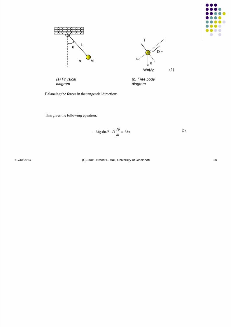
Free Body Diagram

The analysis is begun by drawing afree body diagram of the forcesacting on the mass. We will use thetangent and normal components todescribe the forces acting on themass. The free body diagramshown and Newton's second law arethen used to derive a differentialequation describing the dynamicresponse of the system.

Forces may be balanced in anydirection, however, a particularlysimple form of the equation forpendulum motion can be developed

by balancing the forces in thetangential direction:

s

T

D

W=Mg




s

L

M

(a) Physical

diagram

(b) Free body

diagram

s

T

D

W=Mg

(1)

Balancing the forces in the tangential direction:

This gives the following equation:

Mg Dd

dt Mat sin

(2)




adv

dt

d s

dt t

2

2 (3)

s L (4)

a Ld

dt t

2

2

(5)

The tangential acceleration is given in terms of the rate of change of velocity or arc length by the equation:

Since the arc length, s, is given by:

Substituting s into the differential in Equation 3 yields:




Combining Equation 2 and Equation 5 yields:

Note that the unit of each term is force. In English units, W is in lbf , g is in ft./sec2, D is in

lb.sec, L is in feet, is in radians, d/dt is in rad/sec and d2/dt

2 is in rad/sec

2. In international

SI units, M is in kg, g is in m/sec2, D is in kg-m/sec, L is in meters, is in radians, d/dt is in

rad/sec and d2/dt

2 is in rad/sec

2.

This may be rewritten as:

d dt

D ML

d dt

g L

2

20 sin (7)

Mg Dd

dt Ma ML

d

dt t sin

2

2(6)




System

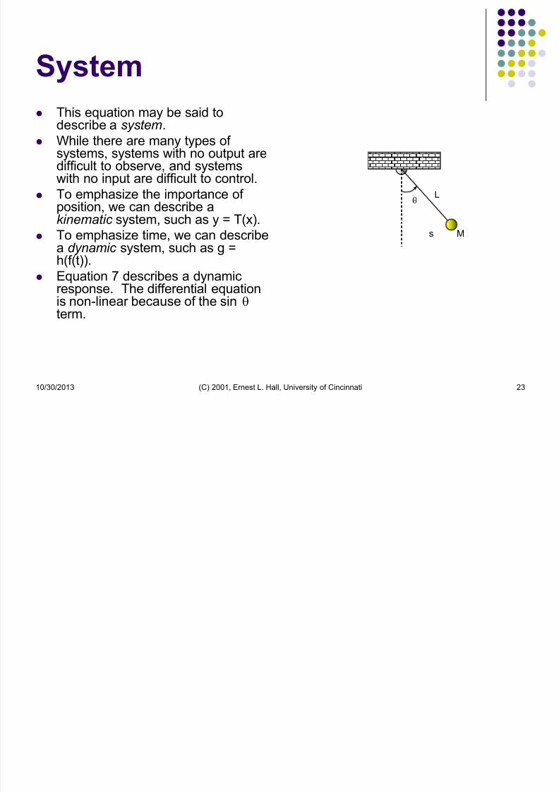
This equation may be said todescribe a system.

While there are many types ofsystems, systems with no output aredifficult to observe, and systemswith no input are difficult to control.

To emphasize the importance ofposition, we can describe akinematic system, such as y = T(x).

To emphasize time, we can describea dynamic system, such as g =h(f(t)).

Equation 7 describes a dynamic

response. The differential equationis non-linear because of the sin term.

s

L

M




For a linear system, y = T (x), two conditions must be satisfied:

1. If a constant, a, is multiplied by the input, x, such that ax is applied as the input, then

the output must be multiplied by the same constant, as in Equation 8:

2. If the sum of two inputs is applied, the output must be the sum of the individual

outputs and the principal of superposition must hold as demonstrated by the following

equations:

where

and

T x y( )2 2 (11)

T x x y y( )1 2 1 2 (9)

T ax ay( ) (8)

T x y( )1 1 (10)




This may be rewritten as:

d

dt

D

ML

d

dt

g

L

2

20

sin (7)

Equation 7 is non-linear because the sine of the sum of two angles is not equal to the sum of

the sines of the two angles. For example, sin(45) = 0.707 while sin(90) = 1.




Linear approach modeling

Returning to the pendulum example, the solution to this non-linear equation with D=0

involves the elliptic function. (The solutions of this non-linear system will be investigated

later using Simulink.) Using the approximation sin = in Equation 7 gives the linear

approximation:

d

dt

D

ML

d

dt

g

L

2

20

(27)




Simple Harmonic Motion

When D=0, Equation 27 simplifies to the linear differential equation for simple harmonic

motion:

d

dt

g

L

2

20

(28)




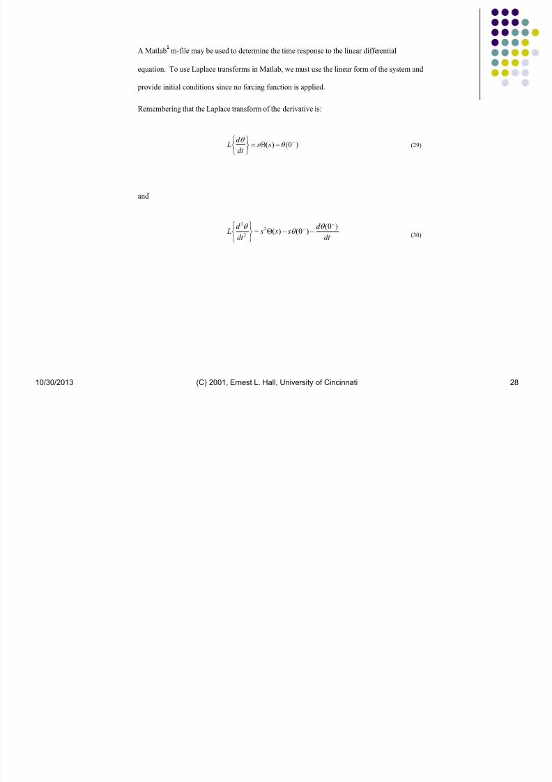
Matlab m-file may be used to determine the time response to the linear differential

equation. To use Laplace transforms in Matlab, we must use the linear form of the system and

provide initial conditions since no forcing function is applied.

Remembering that the Laplace transform of the derivative is:

and

(29))0()(

s sdt

d L

(30)dt

d s s s

dt

d L

)0()0()(2

2

2




Taking the Laplace transform of the linear differential Equation 27 gives:

This may be simplified to:

(31) s s sd

dt

D

ML s s

g

L s2 0

00 0 ( ) ( )

( )( ) ( ) ( )

(32)( )( ) ( )

( )

s s

D

ML

d

dt

s D

ML s

g

L

0 00

2




(Note that the initial conditions act as a forcing function for the system to start it moving.) It is

more common to apply a step function to start a system. The unit step function is defined as:

(Note that the unit step function is the integral of the delta function.) It may also be shown

that the Laplace transform of the delta function is 1, and that the Laplace transform of the unit

step function is 1/s.

0

0

0

1)(

t

t

for

for t u

(33)




To use Matlab to solve the transfer function for (t), we must tell Matlab that this is the output

of some system. Since G(s) = H(s)F(s), we can let H(s) = 1 and F(s) = (s). Then the output

will be G(s) = (s), and the impulse function can be used directly. If Matlab does not have an

impulse response but it does have a step response, then a slight manipulation is required.

(Note that the impulse response of system G(s) is the same as the step response of system s

(G(s)).)




The transform function with numerical values substituted is:

( )( . )

. . s

s

s s

45 0 0268

0 0268 10 732

(34)




Note that (0) = 45, and d/dt = 0. We can define T0 = (0) for ease of

typing, and express the numerator and denominator polynomials by their

coefficients as shown by the num and den vectors below.

To develop a Matlab m-file script using the step function, define the parameters

from the problem statement:

T0 =45

D = 0.1

M = 40/32.2

L = 3

G=32.3

num = [T0, D*T0/(M*L), 0];

den = [1, D/(M*L), G/L ];

t= 0:0.1:10;

step(num,den,t);

grid on

title('Time response of the pendulum linear approximation')




This m-file or script may be run using Matlab and should produce an oscillatory output. The

angle starts at 45 degrees at time 0 and goes in the negative direction first, then oscillates to

some positive angle and dampens out. The period, T in seconds (or frequency, f = 1/T in

cycles/second or Hertz) of the response can be compared to the theoretical solution for an

undamped pendulum given in Equation 35 [4]. The is shown in Figure 3.

T L

g 2

(35)




Now try it!

Use Matlab to solve the

pendulum.

Just open a new

workspace in Matlab. Copy the sample

program.

Run the m-file.0 2 4 6 8 10

-50

0

50

Time (Seconds)

me response o pen u um w near approxma on

D e g r e e s

Figure 3. Pendulum response with linear

approximation. (0+)=45




Homework 1

Now capture your Matlab program and output

and format it on a Word page. Put you name

on the page and turn it in to me as your first

homework assignment.

Documents

MCLECTURE1.PPT