Embed Size (px)
Citation preview
© 2011 ANSYS, Inc. September 8, 2011 1
Maxwell and Simplorer Tips and Tricks
Ryan Magargle, PhD
Ansys, Inc.
© 2011 ANSYS, Inc. September 8, 2011 2
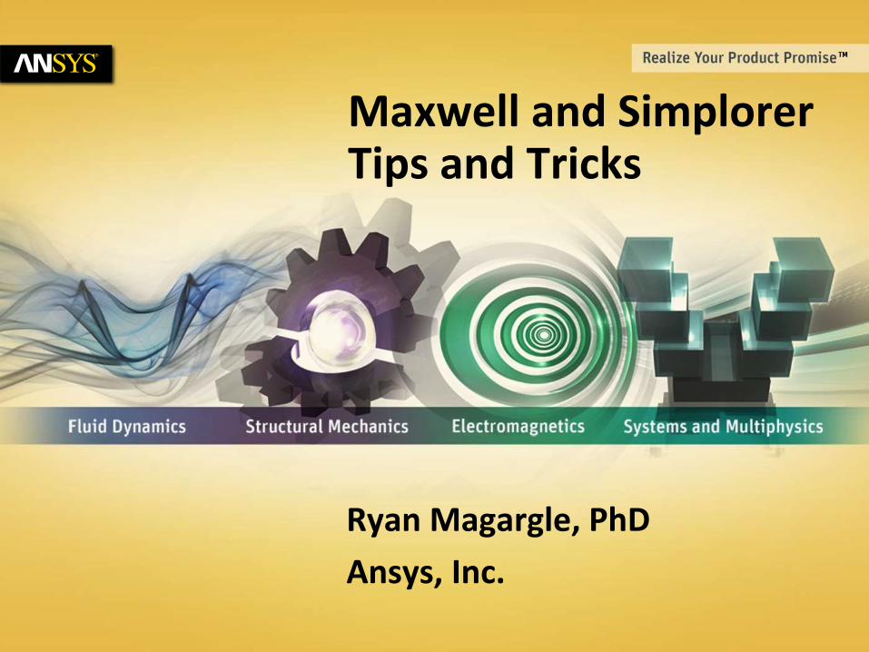
Simplorer System Design
PP := 6
ICA:
A
A
A
GAIN
A
A
A
GAIN
A
JPMSYNCIA
IB
IC
Torque JPMSYNCIA
IB
IC
Torque
D2D
Maxwell 2-D/3-D Electromagnetic Components
PExprt Magnetics
RMxprt Motor Design
Q3D
Parasitics
ANSYS
Mechanical Thermal/Stress
ANSYS Icepack
Model order Reduction
Co-simulation
Field Solution
Model Generation
Electromechanical Simulation
© 2011 ANSYS, Inc. September 8, 2011 3
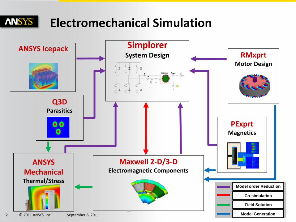
Maxwell Description
Pro
ject
Man
ager
P
rop
erti
es W
ind
ow
Message Manager Progress Window
Modeler Window
Solution Type
Post-Processing
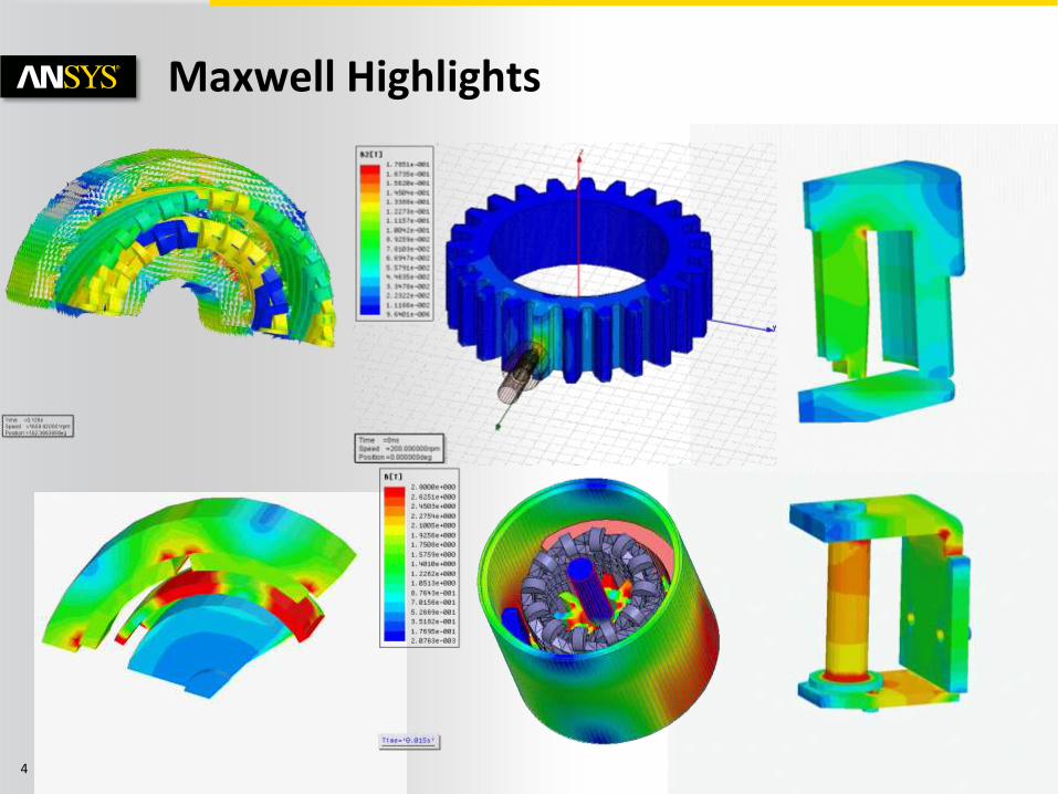
© 2011 ANSYS, Inc. September 8, 2011 4
Maxwell Highlights
© 2011 ANSYS, Inc. September 8, 2011 5
Outline
Maxwell
– Geometry
– Transient
– Post-Processing
Simplorer
– Transient Solver
– Post-Processing
– Advanced Analysis
© 2011 ANSYS, Inc. September 8, 2011 6
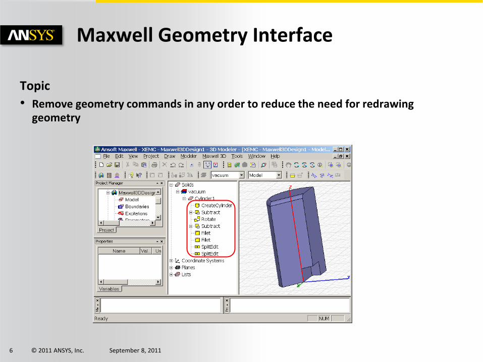
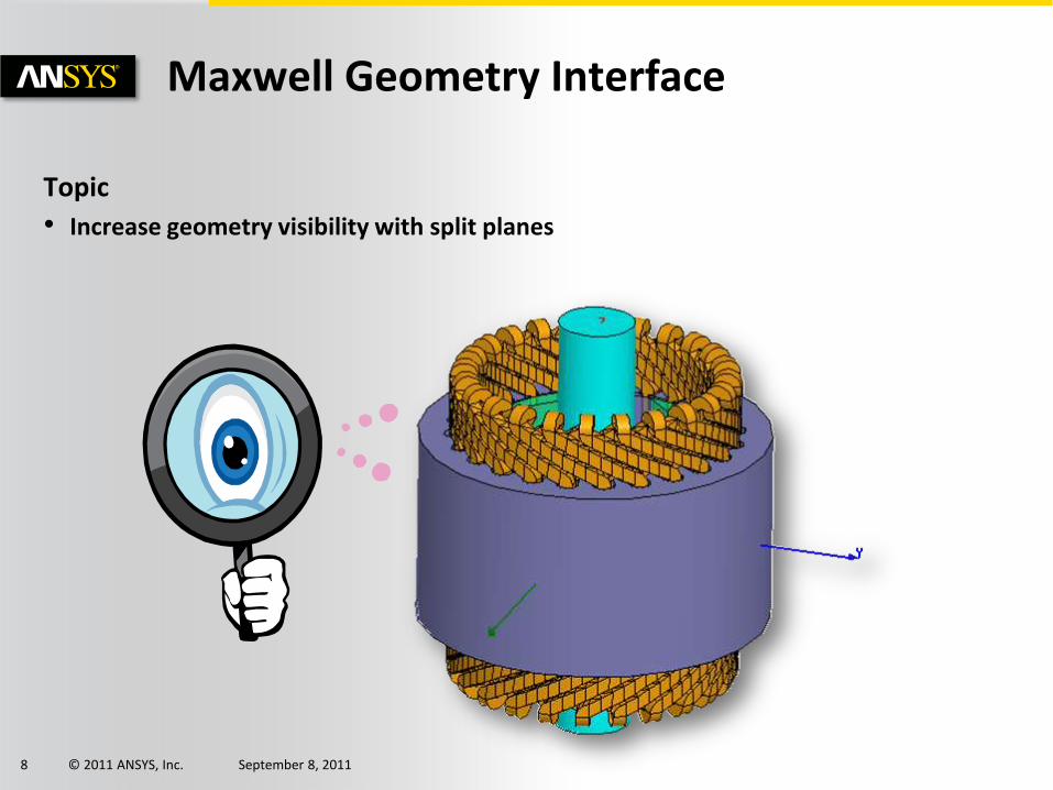
Maxwell Geometry Interface
Topic
• Remove geometry commands in any order to reduce the need for redrawing geometry
© 2011 ANSYS, Inc. September 8, 2011 7
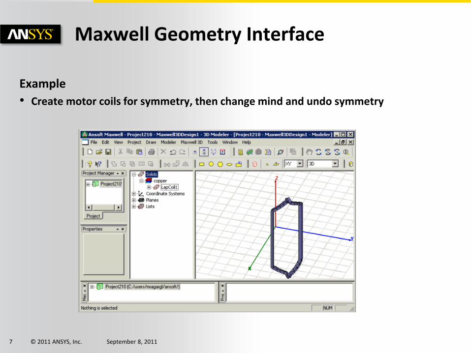
Maxwell Geometry Interface
Example
• Create motor coils for symmetry, then change mind and undo symmetry
© 2011 ANSYS, Inc. September 8, 2011 8
Maxwell Geometry Interface
Topic
• Increase geometry visibility with split planes
© 2011 ANSYS, Inc. September 8, 2011 9
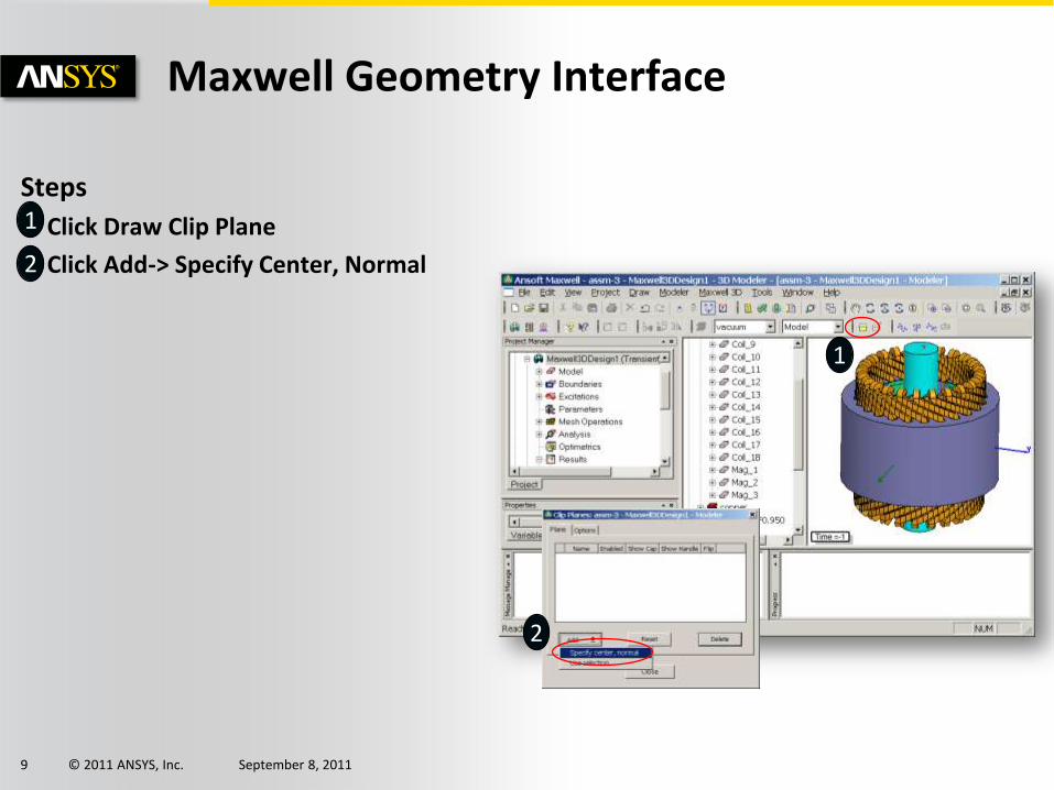
Maxwell Geometry Interface
Steps
• Click Draw Clip Plane
• Click Add-> Specify Center, Normal
1
2
1
2
© 2011 ANSYS, Inc. September 8, 2011 10
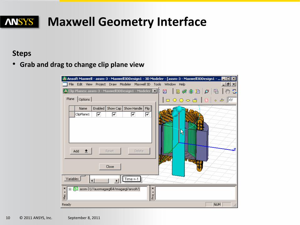
Maxwell Geometry Interface
Steps
• Grab and drag to change clip plane view
© 2011 ANSYS, Inc. September 8, 2011 11
Outline
Maxwell
– Geometry
– Transient
– Post-Processing
Simplorer
– Transient Solver
– Post-Processing
– Advanced Analysis
© 2011 ANSYS, Inc. September 8, 2011 12
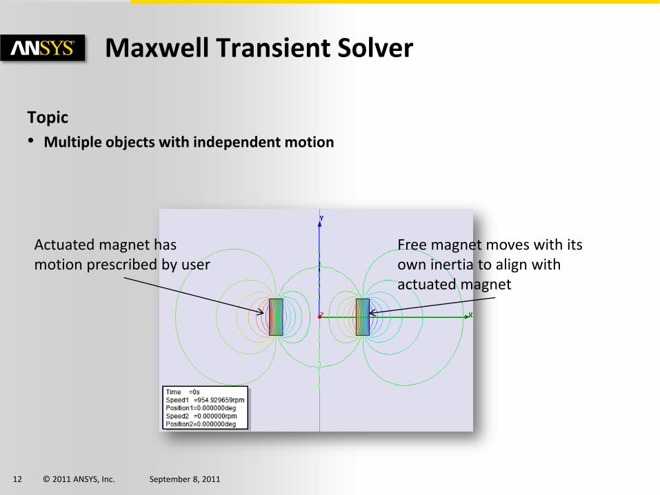
Maxwell Transient Solver
Topic
• Multiple objects with independent motion
Actuated magnet has motion prescribed by user
Free magnet moves with its own inertia to align with actuated magnet
© 2011 ANSYS, Inc. September 8, 2011 13
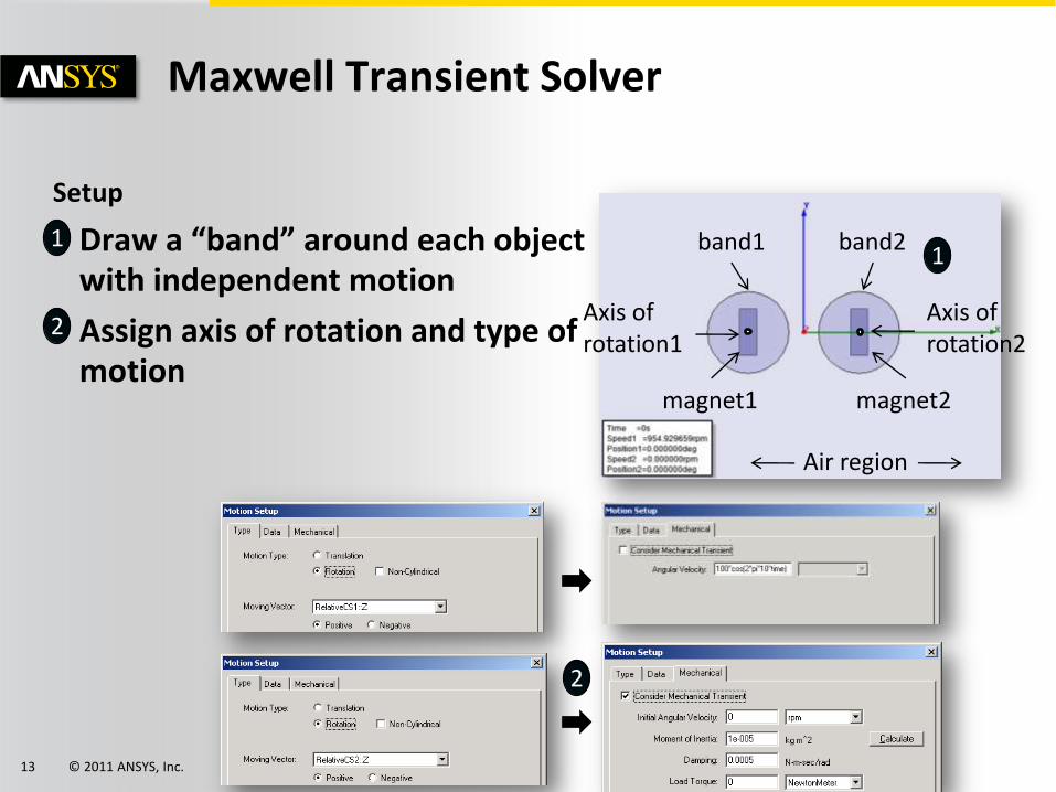
Maxwell Transient Solver
Setup
• Draw a “band” around each object with independent motion
• Assign axis of rotation and type of motion
Air region
band1 band2
magnet1 magnet2
Axis of rotation1
Axis of rotation2
1
2
1
2
© 2011 ANSYS, Inc. September 8, 2011 14
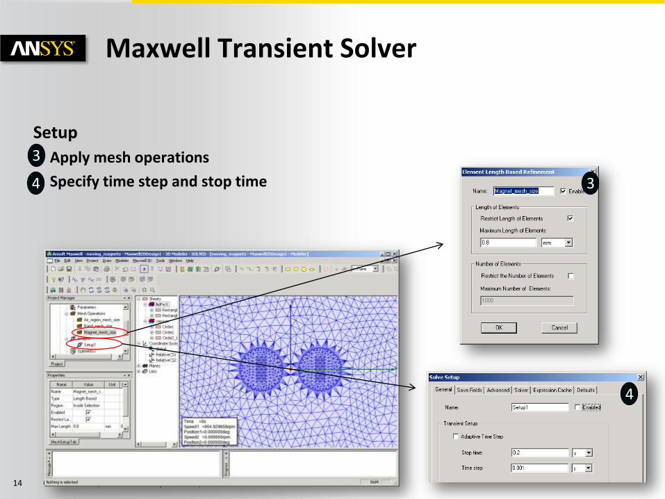
Maxwell Transient Solver
Setup
• Apply mesh operations
• Specify time step and stop time 3
4
3
4
© 2011 ANSYS, Inc. September 8, 2011 15
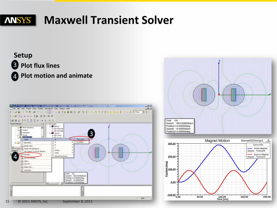
Maxwell Transient Solver
Setup
• Plot flux lines
• Plot motion and animate
3
4
0.00 50.00 100.00 150.00 200.00Time [ms]
-100.00
0.00
100.00
200.00
300.00
Po
sit
ion
[d
eg
]
Maxwell2DDesign1Magnet Motion ANSOFT
Curve Info
Victim MagnetSetup1 : Transient
Source MagnetSetup1 : Transient
3
4
© 2011 ANSYS, Inc. September 8, 2011 16
Maxwell Transient Solver
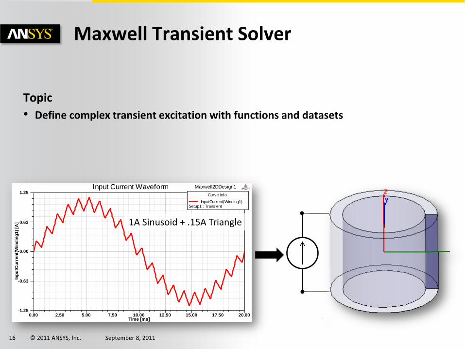
Topic
• Define complex transient excitation with functions and datasets
0.00 2.50 5.00 7.50 10.00 12.50 15.00 17.50 20.00Time [ms]
-1.25
-0.63
0.00
0.63
1.25
Inp
utC
urr
en
t(W
ind
ing
1)
[A]
Maxwell2DDesign1Input Current Waveform ANSOFT
Curve Info
InputCurrent(Winding1)Setup1 : Transient
1A Sinusoid + .15A Triangle
© 2011 ANSYS, Inc. September 8, 2011 17
Maxwell Transient Solver
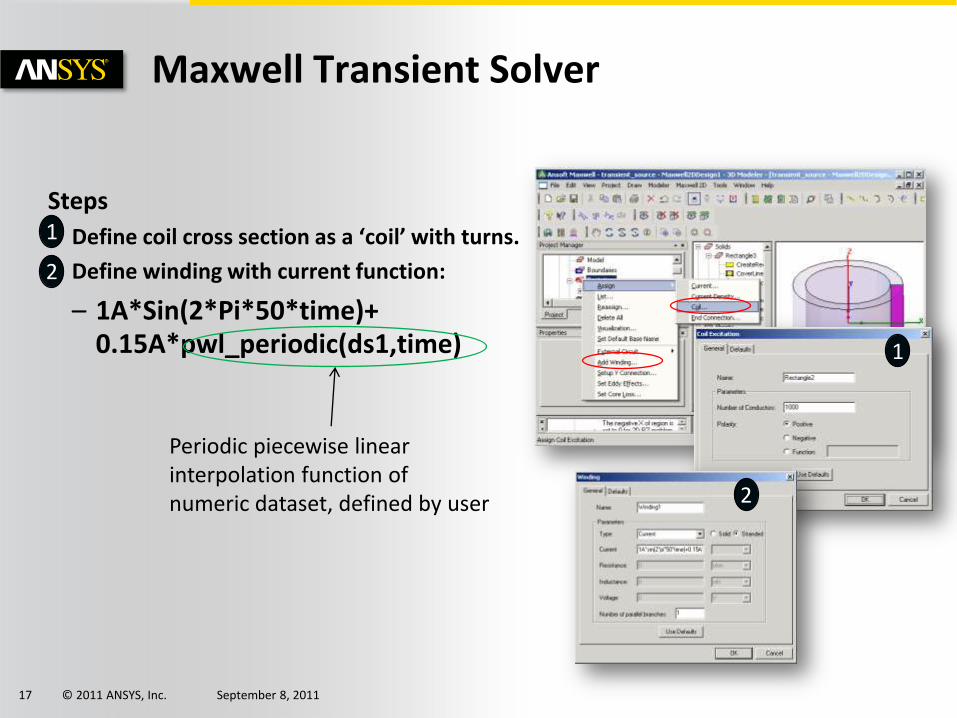
Steps
• Define coil cross section as a ‘coil’ with turns.
• Define winding with current function:
– 1A*Sin(2*Pi*50*time)+ 0.15A*pwl_periodic(ds1,time) 1
2
Periodic piecewise linear interpolation function of numeric dataset, defined by user
1
2
© 2011 ANSYS, Inc. September 8, 2011 18
Maxwell Transient Solver
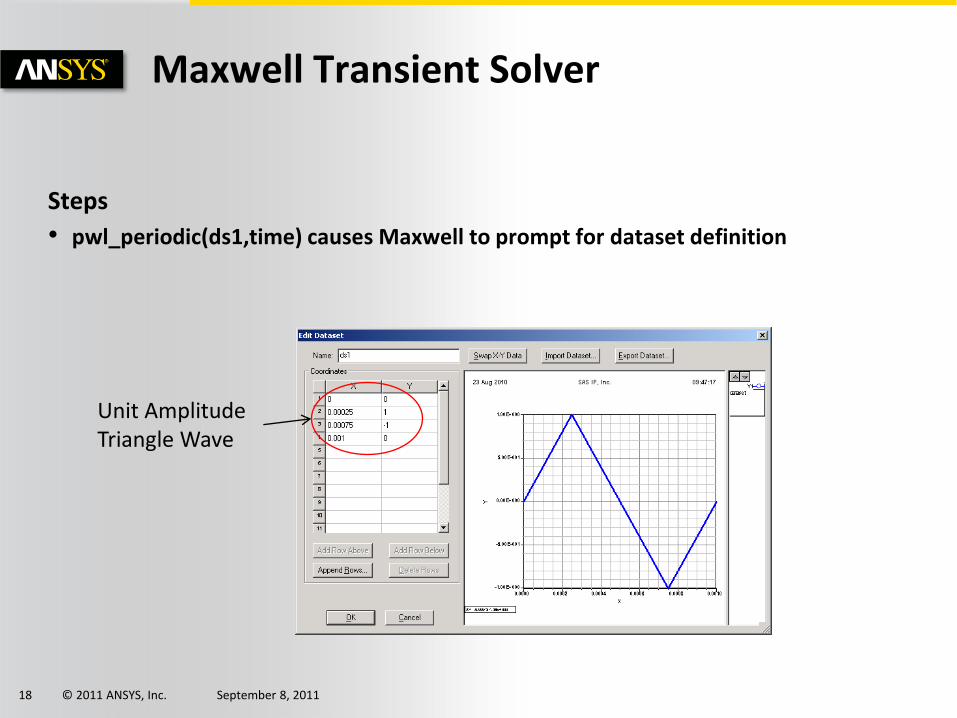
Steps
• pwl_periodic(ds1,time) causes Maxwell to prompt for dataset definition
Unit Amplitude Triangle Wave
© 2011 ANSYS, Inc. September 8, 2011 19
Maxwell Transient Solver
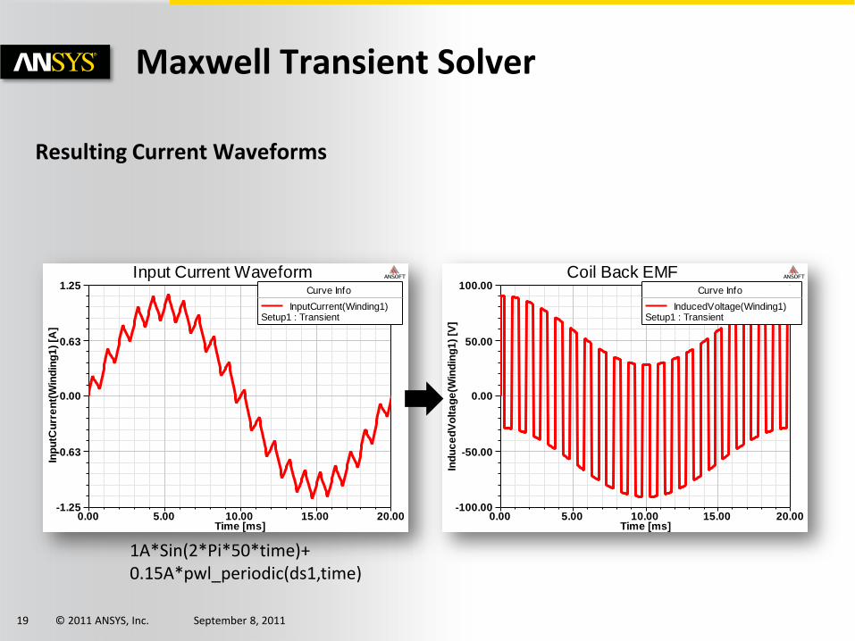
Resulting Current Waveforms
0.00 5.00 10.00 15.00 20.00Time [ms]
-100.00
-50.00
0.00
50.00
100.00
Ind
uc
ed
Vo
lta
ge
(Win
din
g1
) [V
]
Coil Back EMF ANSOFT
Curve Info
InducedVoltage(Winding1)Setup1 : Transient
0.00 5.00 10.00 15.00 20.00Time [ms]
-1.25
-0.63
0.00
0.63
1.25
Inp
utC
urr
en
t(W
ind
ing
1)
[A]
Input Current Waveform ANSOFT
Curve Info
InputCurrent(Winding1)Setup1 : Transient
1A*Sin(2*Pi*50*time)+ 0.15A*pwl_periodic(ds1,time)
© 2011 ANSYS, Inc. September 8, 2011 20
Maxwell Transient Solver
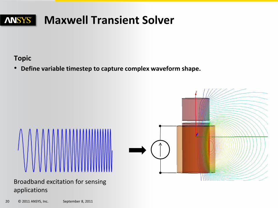
Topic
• Define variable timestep to capture complex waveform shape.
Broadband excitation for sensing applications
© 2011 ANSYS, Inc. September 8, 2011 21
Maxwell Transient Solver
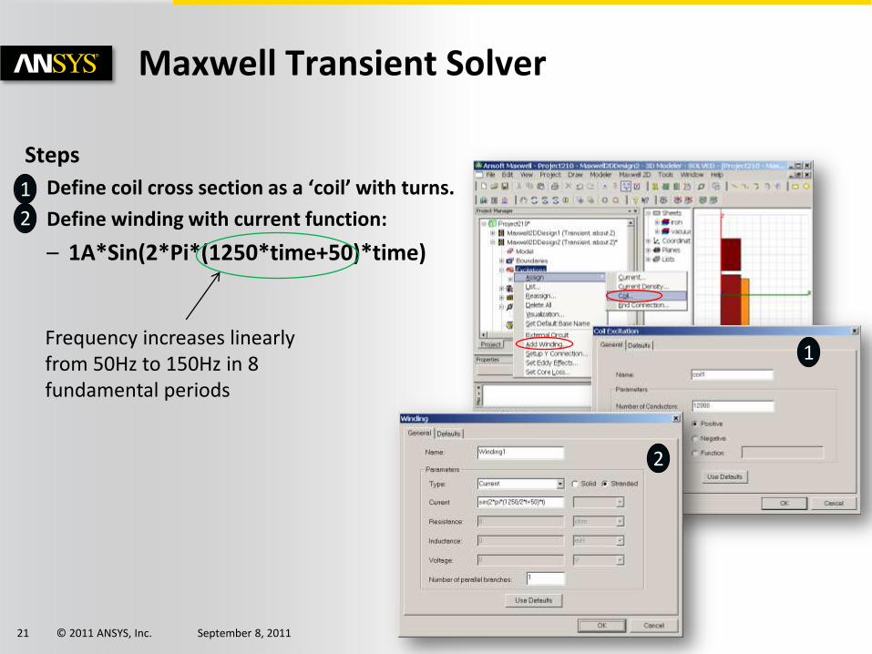
Steps
• Define coil cross section as a ‘coil’ with turns.
• Define winding with current function:
– 1A*Sin(2*Pi*(1250*time+50)*time)
Frequency increases linearly from 50Hz to 150Hz in 8 fundamental periods
1
2
1
2
© 2011 ANSYS, Inc. September 8, 2011 22
Maxwell Transient Solver
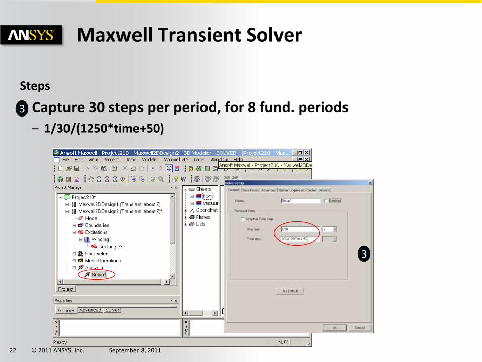
Steps
• Capture 30 steps per period, for 8 fund. periods – 1/30/(1250*time+50)
3
3
© 2011 ANSYS, Inc. September 8, 2011 23
Outline
Maxwell
– Geometry
– Transient
– Post-Processing
Simplorer
– Transient Solver
– Post-Processing
– Advanced Analysis
© 2011 ANSYS, Inc. September 8, 2011 24
Maxwell Post-Processing
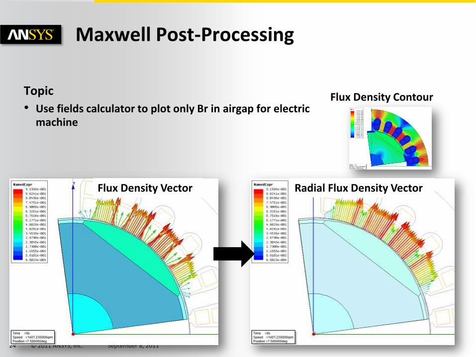
Topic
• Use fields calculator to plot only Br in airgap for electric machine
Flux Density Contour
Flux Density Vector Radial Flux Density Vector
© 2011 ANSYS, Inc. September 8, 2011 25
Maxwell Post-Processing
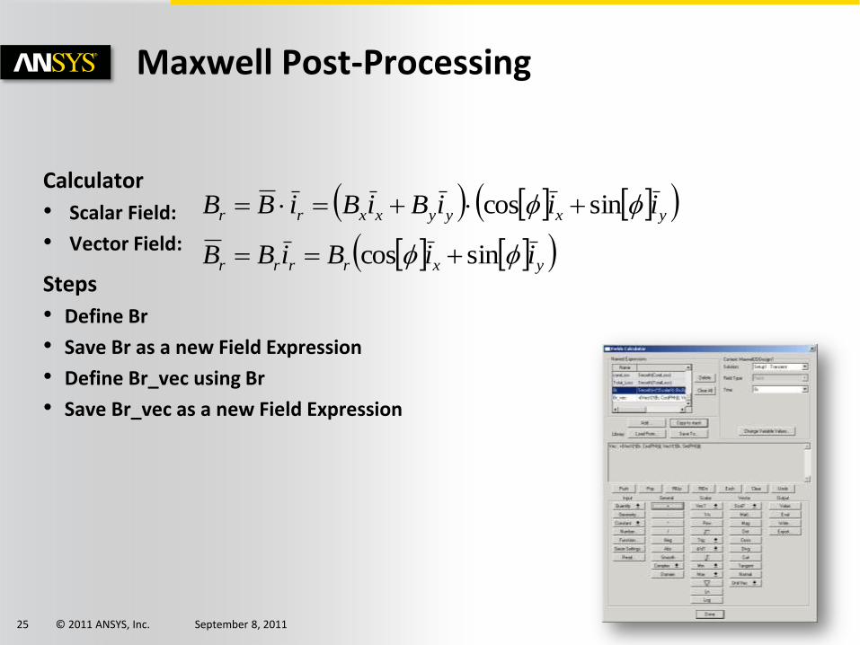
Calculator
• Scalar Field:
• Vector Field:
Steps
• Define Br
• Save Br as a new Field Expression
• Define Br_vec using Br
• Save Br_vec as a new Field Expression
yxyyxxrr iiiBiBiBB sincos
yxrrrr iiBiBB sincos
© 2011 ANSYS, Inc. September 8, 2011 26
Maxwell Post-Processing
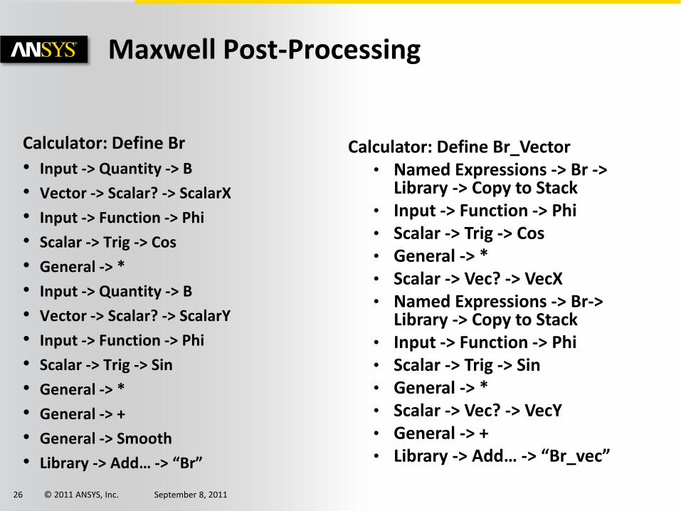
Calculator: Define Br
• Input -> Quantity -> B
• Vector -> Scalar? -> ScalarX
• Input -> Function -> Phi
• Scalar -> Trig -> Cos
• General -> *
• Input -> Quantity -> B
• Vector -> Scalar? -> ScalarY
• Input -> Function -> Phi
• Scalar -> Trig -> Sin
• General -> *
• General -> +
• General -> Smooth
• Library -> Add… -> “Br”
Calculator: Define Br_Vector • Named Expressions -> Br ->
Library -> Copy to Stack • Input -> Function -> Phi • Scalar -> Trig -> Cos • General -> * • Scalar -> Vec? -> VecX • Named Expressions -> Br->
Library -> Copy to Stack • Input -> Function -> Phi • Scalar -> Trig -> Sin • General -> * • Scalar -> Vec? -> VecY • General -> + • Library -> Add… -> “Br_vec”
© 2011 ANSYS, Inc. September 8, 2011 27
Maxwell Post-Processing
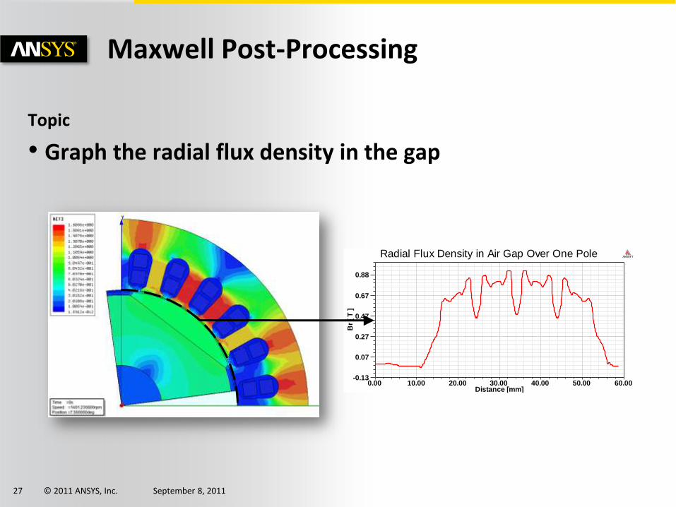
Topic
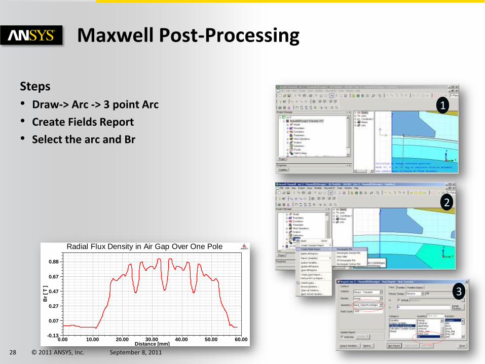
• Graph the radial flux density in the gap
0.00 10.00 20.00 30.00 40.00 50.00 60.00Distance [mm]
-0.13
0.07
0.27
0.47
0.67
0.88
Br
[ T
]
Radial Flux Density in Air Gap Over One Pole ANSOFT
© 2011 ANSYS, Inc. September 8, 2011 28
Maxwell Post-Processing
Steps
• Draw-> Arc -> 3 point Arc
• Create Fields Report
• Select the arc and Br
1
2
3
0.00 10.00 20.00 30.00 40.00 50.00 60.00Distance [mm]
-0.13
0.07
0.27
0.47
0.67
0.88
Br
[ T
]
Radial Flux Density in Air Gap Over One Pole ANSOFT
© 2011 ANSYS, Inc. September 8, 2011 29
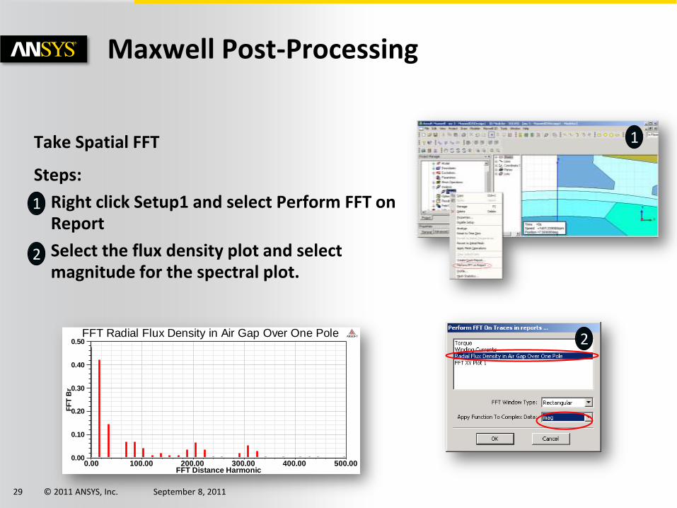
Maxwell Post-Processing
Take Spatial FFT
Steps:
• Right click Setup1 and select Perform FFT on Report
• Select the flux density plot and select magnitude for the spectral plot.
1
2
0.00 100.00 200.00 300.00 400.00 500.00FFT Distance Harmonic
0.00
0.10
0.20
0.30
0.40
0.50
FF
T B
r
FFT Radial Flux Density in Air Gap Over One Pole ANSOFT
1
2
© 2011 ANSYS, Inc. September 8, 2011 30
-60.00 -40.00 -20.00 0.00 20.00 40.00H [A / m] [kA_per_m]
0.00
0.20
0.40
0.60
0.80
1.00
1.20
1.40
B [
T ]
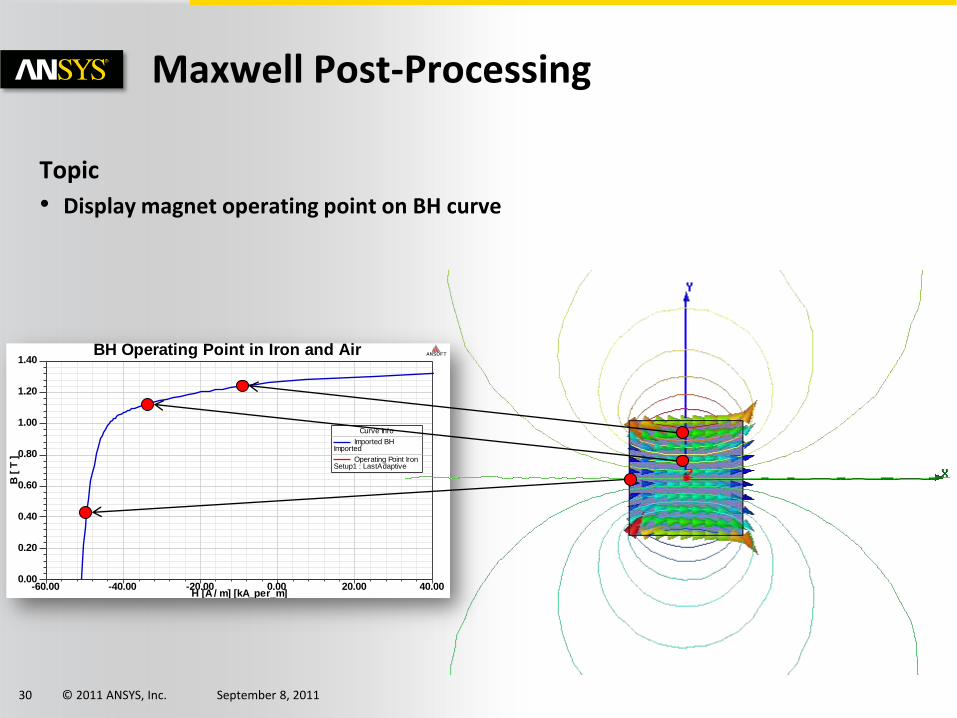
BH Operating Point in Iron and Air ANSOFT
Curve Info
Imported BHImported
Operating Point IronSetup1 : LastAdaptive
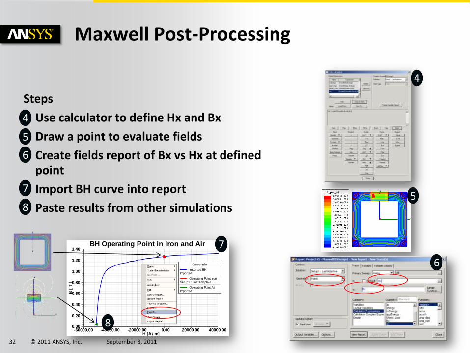
Maxwell Post-Processing
Topic
• Display magnet operating point on BH curve
© 2011 ANSYS, Inc. September 8, 2011 31
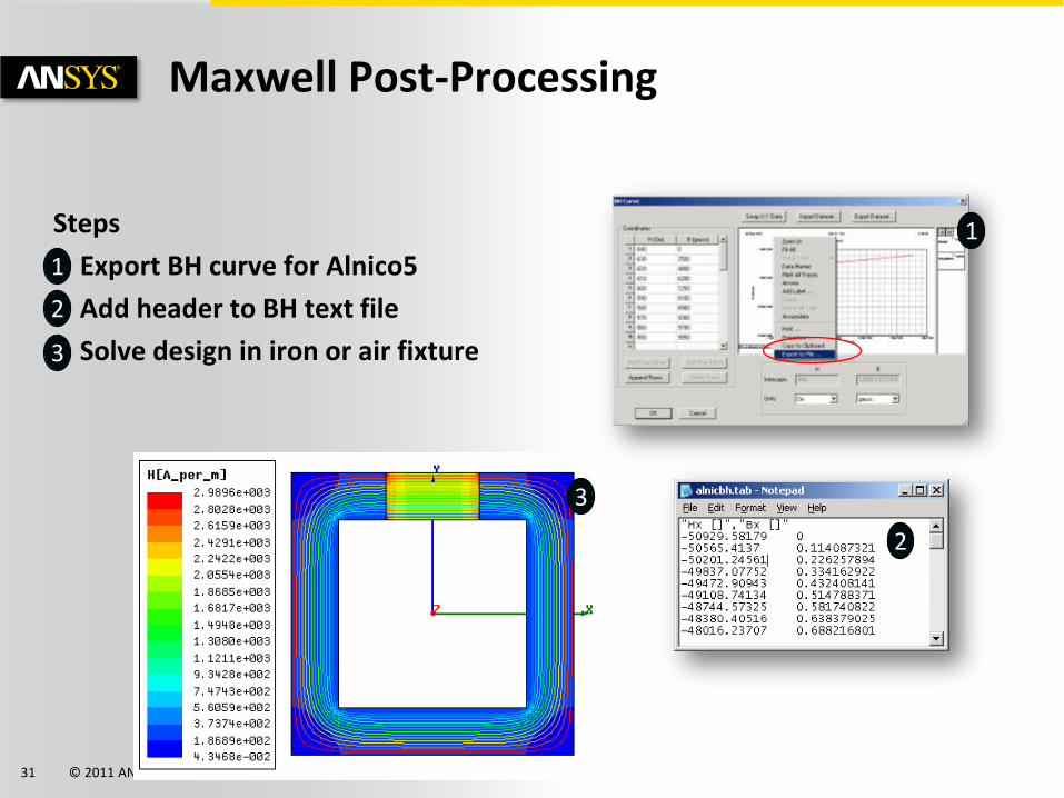
Maxwell Post-Processing
Steps
• Export BH curve for Alnico5
• Add header to BH text file
• Solve design in iron or air fixture
1
2
3
1
2
3
© 2011 ANSYS, Inc. September 8, 2011 32
-60000.00 -40000.00 -20000.00 0.00 20000.00 40000.00H [A / m]
0.00
0.20
0.40
0.60
0.80
1.00
1.20
1.40
B [
T ]
BH Operating Point in Iron and Air ANSOFT
Curve Info
Imported BHImported
Operating Point IronSetup1 : LastAdaptive
Operating Point AirImported
Maxwell Post-Processing
Steps
• Use calculator to define Hx and Bx
• Draw a point to evaluate fields
• Create fields report of Bx vs Hx at defined point
• Import BH curve into report
• Paste results from other simulations 5
4
6
7
8
5
4
6
7
8
© 2011 ANSYS, Inc. September 8, 2011 33
Outline
Maxwell
– Geometry
– Transient
– Post-Processing
Simplorer
– Transient Solver
– Post-Processing
– Advanced Analysis
© 2011 ANSYS, Inc. September 8, 2011 34
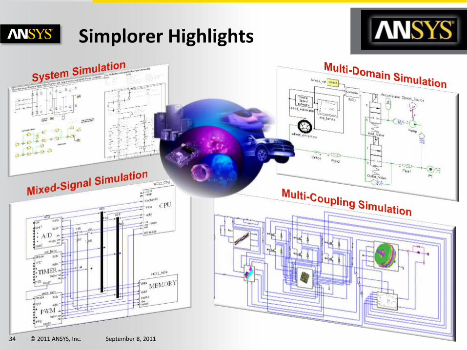
Simplorer Highlights
© 2011 ANSYS, Inc. September 8, 2011 35
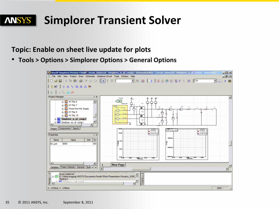
Simplorer Transient Solver
Topic: Enable on sheet live update for plots
• Tools > Options > Simplorer Options > General Options
© 2011 ANSYS, Inc. September 8, 2011 37
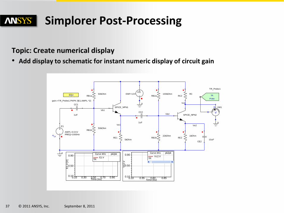
Simplorer Post-Processing
Topic: Create numerical display
• Add display to schematic for instant numeric display of circuit gain
0
0
0
E1
AMPL=0.01V
FREQ=1000Hz
VccEMF=12V
RB1a50kOhm
RE15kOhm
RB2a100kOhm
RB2b22kOhm
RE21kOhm
SPICE_NPN1
SPICE_NPN2
CC1
1uF
CC2
1uF
+
V
VM1
TR
Probe
TR_Probe1
EQU
gain:=TR_Probe1.PKPK /(E1.AMPL *2)
RB1b50kOhm
RC2RC
CE210uF
Vb1
Ve1 Ve2
Vc2
Vb2
0.10 0.30 0.50 0.70 0.90Time [ns]
0.10
0.50
0.90
E1
.V [V
]
Curve Info pk2pk
E1.VTR
0.10 0.35 0.60 0.85Time [ns]
0.10
0.50
0.90
Vc2
.V
Curve Info pk2pk
Vc2.VTR
© 2011 ANSYS, Inc. September 8, 2011 38
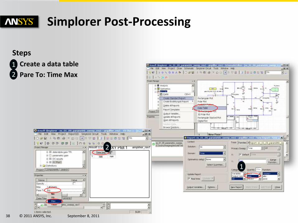
Simplorer Post-Processing
Steps
• Create a data table
• Pare To: Time Max
1
2
1
2
© 2011 ANSYS, Inc. September 8, 2011 39
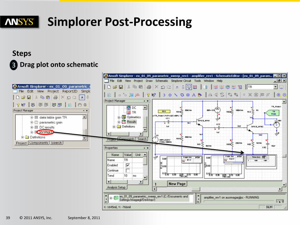
Simplorer Post-Processing
Steps
• Drag plot onto schematic 3
© 2011 ANSYS, Inc. September 8, 2011 40
Outline
Maxwell
– Geometry
– Transient
– Post-Processing
Simplorer
– Transient Solver
– Post-Processing
– Advanced Analysis
© 2011 ANSYS, Inc. September 8, 2011 41
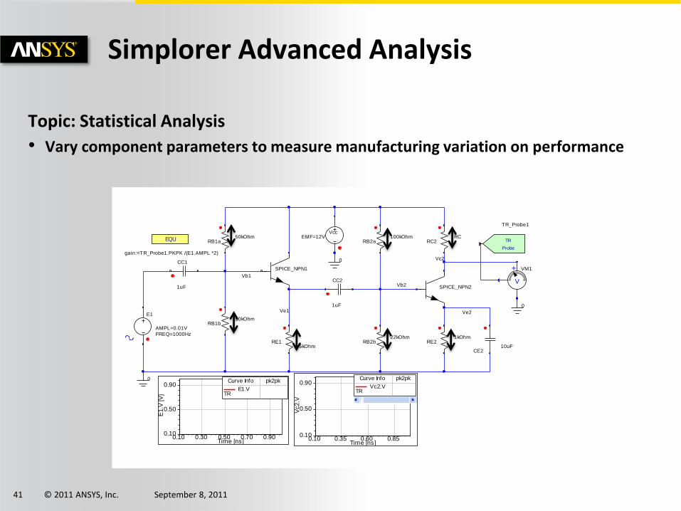
Simplorer Advanced Analysis
Topic: Statistical Analysis
• Vary component parameters to measure manufacturing variation on performance
0
0
0
E1
AMPL=0.01V
FREQ=1000Hz
VccEMF=12V
RB1a50kOhm
RE15kOhm
RB2a100kOhm
RB2b22kOhm
RE21kOhm
SPICE_NPN1
SPICE_NPN2
CC1
1uF
CC2
1uF
+
V
VM1
TR
Probe
TR_Probe1
EQU
gain:=TR_Probe1.PKPK /(E1.AMPL *2)
RB1b50kOhm
RC2RC
CE210uF
Vb1
Ve1 Ve2
Vc2
Vb2
0.10 0.30 0.50 0.70 0.90Time [ns]
0.10
0.50
0.90
E1
.V [V
]
Curve Info pk2pk
E1.VTR
0.10 0.35 0.60 0.85Time [ns]
0.10
0.50
0.90
Vc2
.V
Curve Info pk2pk
Vc2.VTR
© 2011 ANSYS, Inc. September 8, 2011 42
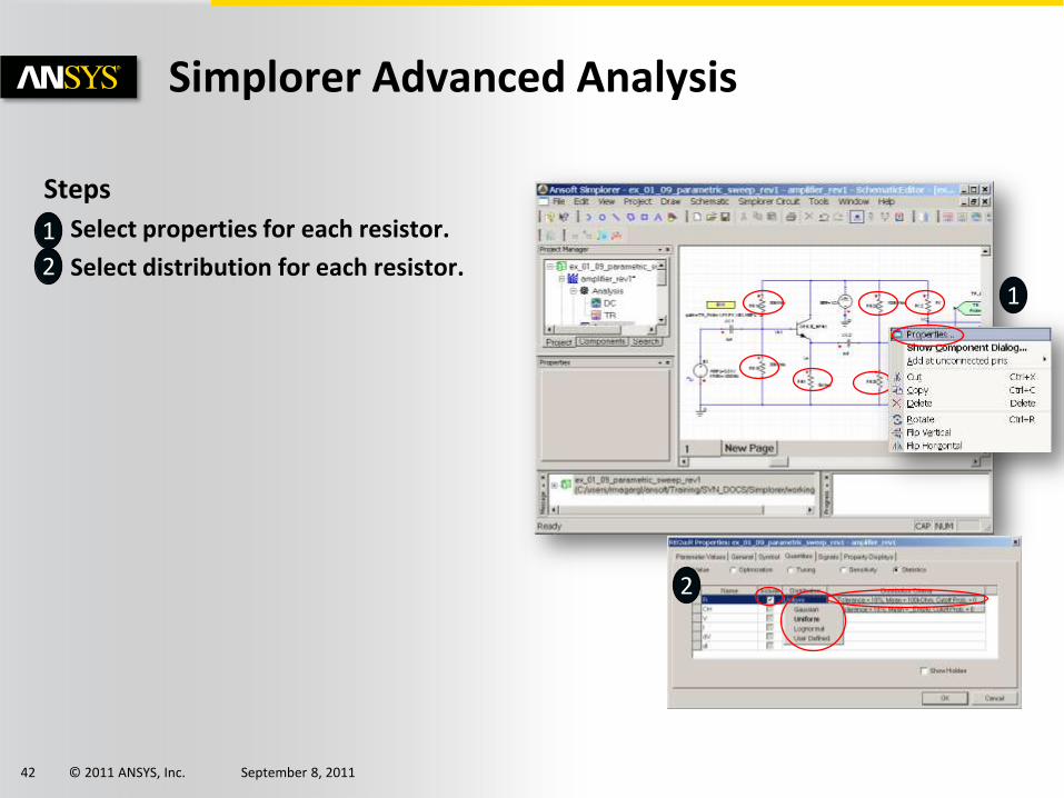
Simplorer Advanced Analysis
Steps
• Select properties for each resistor.
• Select distribution for each resistor.
1
1
2
2
© 2011 ANSYS, Inc. September 8, 2011 43
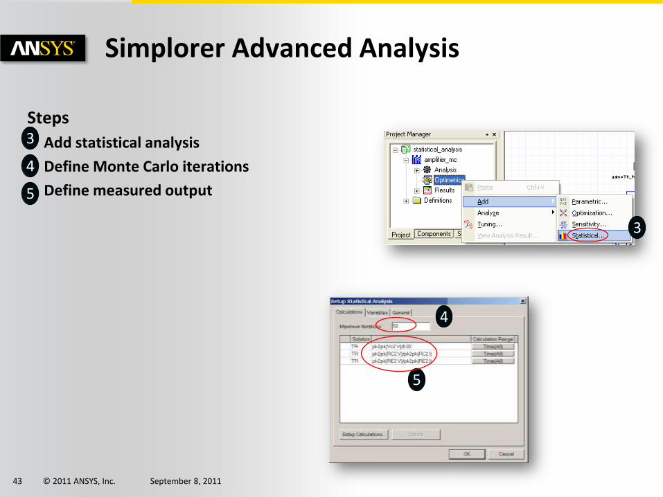
Simplorer Advanced Analysis
Steps
• Add statistical analysis
• Define Monte Carlo iterations
• Define measured output
3
4
5
3
5
4
© 2011 ANSYS, Inc. September 8, 2011 44
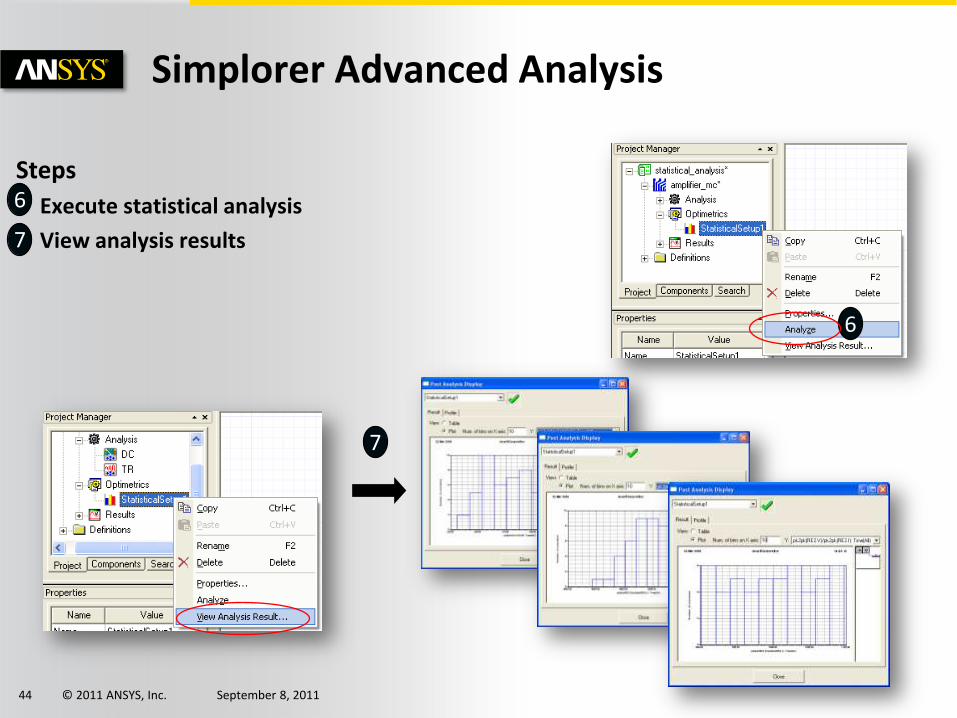
Simplorer Advanced Analysis
Steps
• Execute statistical analysis
• View analysis results
6
7
6
7
© 2011 ANSYS, Inc. September 8, 2011 45
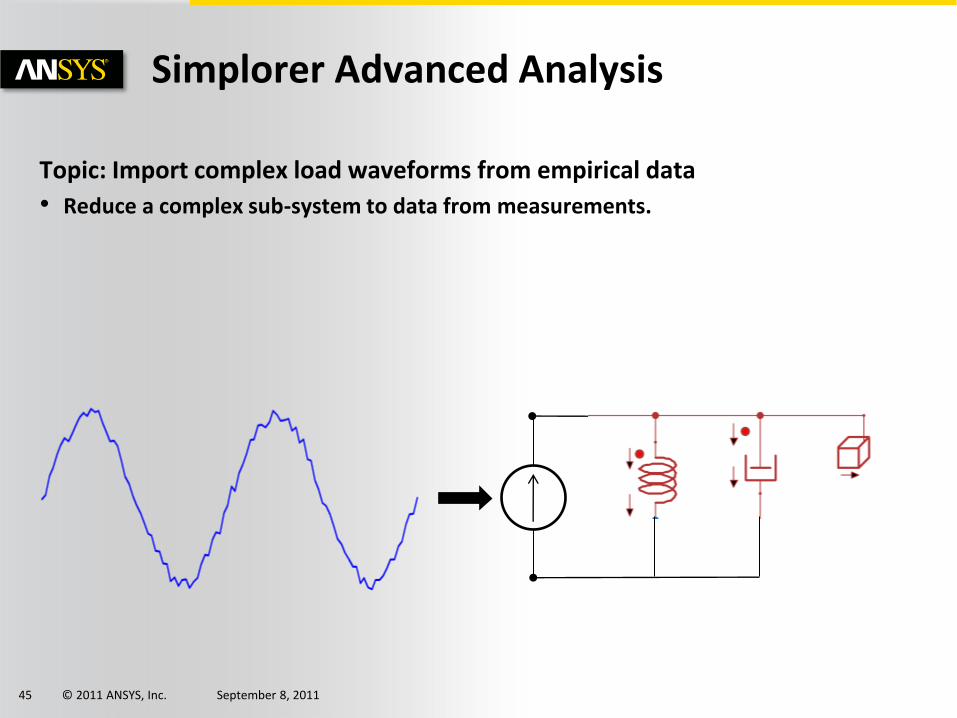
Simplorer Advanced Analysis
Topic: Import complex load waveforms from empirical data
• Reduce a complex sub-system to data from measurements.
© 2011 ANSYS, Inc. September 8, 2011 46
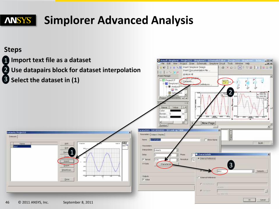
Simplorer Advanced Analysis
Steps
• Import text file as a dataset
• Use datapairs block for dataset interpolation
• Select the dataset in (1)
1
1
2
2
3
3
© 2011 ANSYS, Inc. September 8, 2011 47
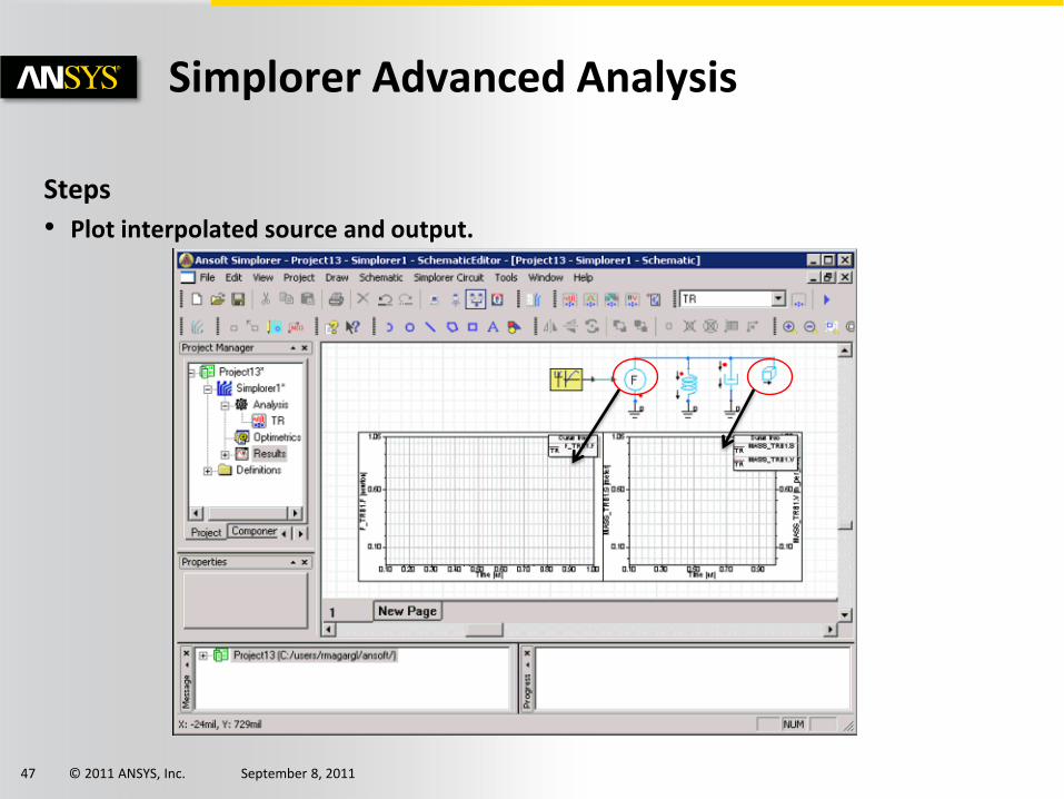
Simplorer Advanced Analysis
Steps
• Plot interpolated source and output.
© 2011 ANSYS, Inc. September 8, 2011 48
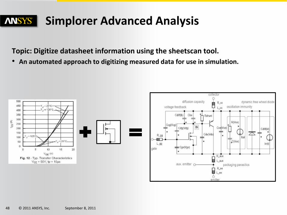
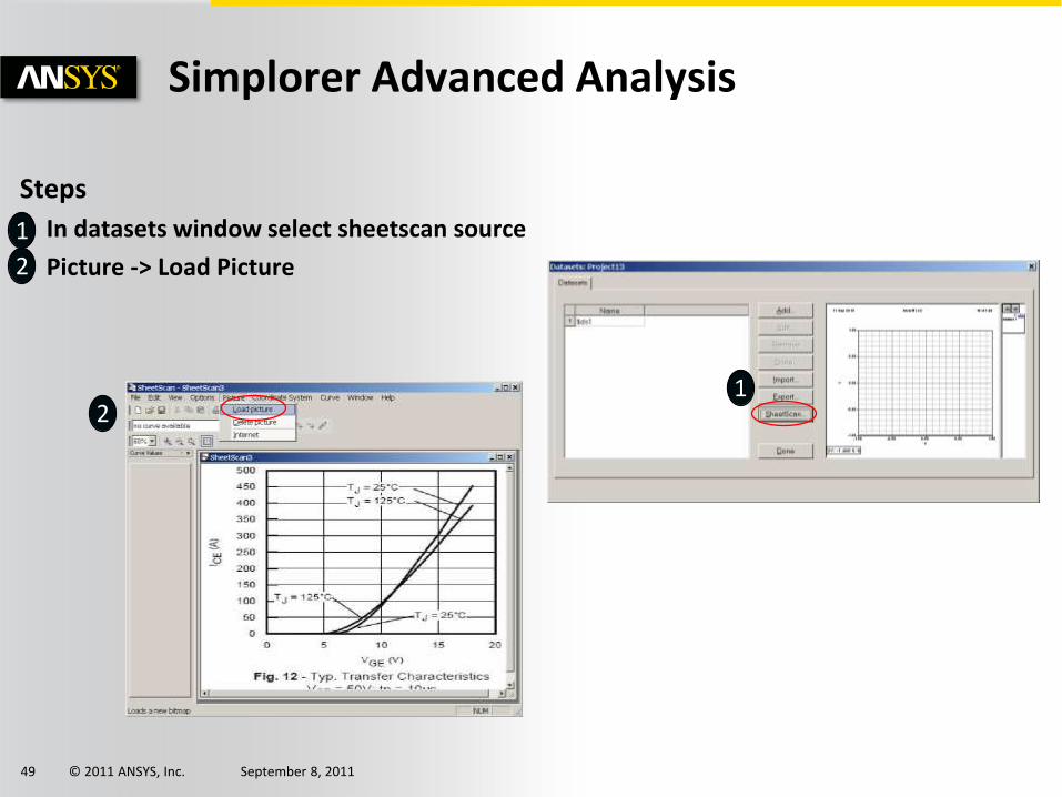
Simplorer Advanced Analysis
Topic: Digitize datasheet information using the sheetscan tool.
• An automated approach to digitizing measured data for use in simulation.
© 2011 ANSYS, Inc. September 8, 2011 49
Simplorer Advanced Analysis
Steps
• In datasets window select sheetscan source
• Picture -> Load Picture
1
2
1 2
© 2011 ANSYS, Inc. September 8, 2011 50
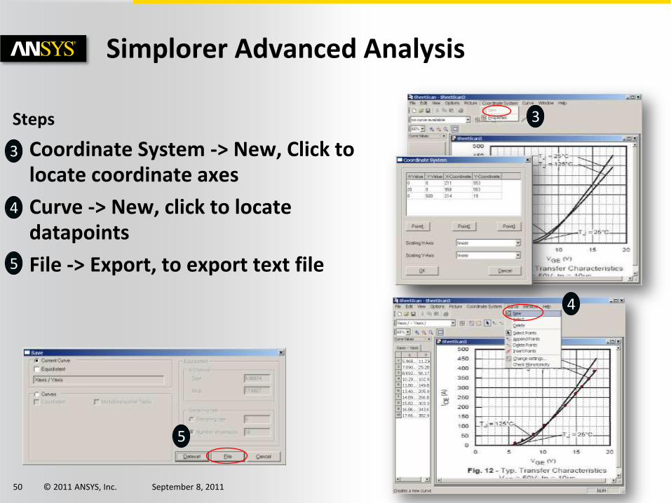
Simplorer Advanced Analysis
Steps
• Coordinate System -> New, Click to locate coordinate axes
• Curve -> New, click to locate datapoints
• File -> Export, to export text file
3
4
3
4
5
5
© 2011 ANSYS, Inc. September 8, 2011 51
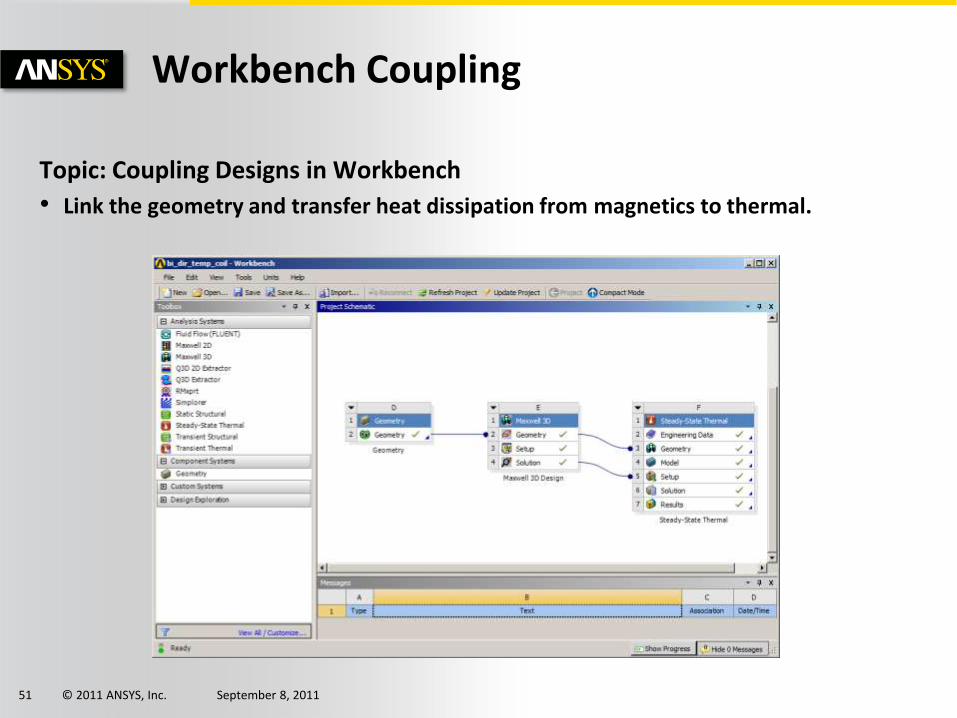
Workbench Coupling
Topic: Coupling Designs in Workbench
• Link the geometry and transfer heat dissipation from magnetics to thermal.
© 2011 ANSYS, Inc. September 8, 2011 52
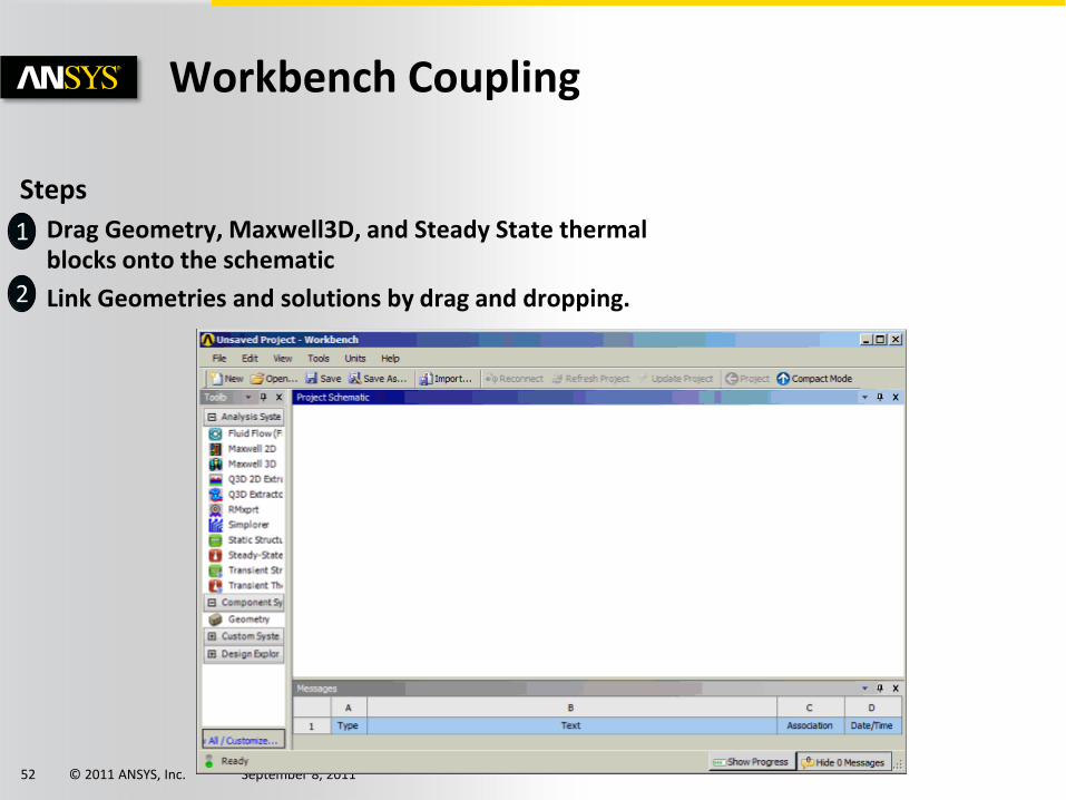
Workbench Coupling
Steps
• Drag Geometry, Maxwell3D, and Steady State thermal blocks onto the schematic
• Link Geometries and solutions by drag and dropping.
1
2
© 2011 ANSYS, Inc. September 8, 2011 53
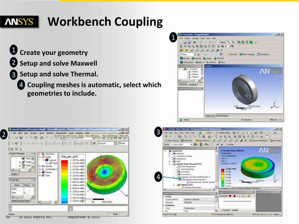
Workbench Coupling
• Create your geometry
• Setup and solve Maxwell
• Setup and solve Thermal.
– Coupling meshes is automatic, select which geometries to include.
1
2
3
4
1
2 3
4

© 2011 ANSYS, Inc. September 8, 2011 54
Questions?