Embed Size (px)
Citation preview
SIAM J. SCI. COMPUT. c! 2014 Society for Industrial and Applied MathematicsVol. 36, No. 5, pp. A2296–A2325
MAXIMUM-PRINCIPLE-SATISFYING THIRD ORDERDISCONTINUOUS GALERKIN SCHEMES FOR FOKKER–PLANCK
EQUATIONS"
HAILIANG LIU† AND HUI YU†
Abstract. We design and analyze up to third order accurate discontinuous Galerkin (DG) meth-ods satisfying a strict maximum principle for Fokker–Planck equations. A procedure is establishedto identify an e!ective test set in each computational cell to ensure the desired bounds of numer-ical averages during time evolution. This is achievable by taking advantage of the two parametersin the numerical flux and a novel decomposition of weighted cell averages. Based on this result,a scaling limiter for the DG method with first order Euler forward time discretization is proposedto solve the one-dimensional Fokker–Planck equations. Strong stability preserving high order timediscretizations will keep the maximum principle. It is straightforward to extend the method to twoand higher dimensions on rectangular meshes. We also show that a modified limiter can preservethe strict maximum principle for DG schemes solving Fokker–Planck equations. As a consequence,the present schemes preserve steady states. Numerical tests for the DG method are reported, withapplications to polymer models with both Hookean and FENE potentials.
Key words. Fokker–Planck equations, discontinuous Galerkin method, maximum principle,high order accuracy, strong stability preserving time discretization
AMS subject classifications. 65M06, 65M60, 65M12
DOI. 10.1137/130935161
1. Introduction. In this paper we are interested in constructing high orderaccurate schemes for solving the initial boundary value problem for Fokker–Planckequations,
(1.1)
!"
#
!tf = !x · (!xf +!xUf), x " B, t > 0,!!f + !!Uf |!B = 0, t > 0,f(0,x) = f0(x), x " B,
where f denotes the probability density function (pdf), U : B # R is a given potential,x is the configuration variable in a bounded domain B $ Rd, and ! is the outwardnormal vector on the boundary !B.
The Fokker–Planck equation in general describes in a statistical sense how acollection of initial data evolves in time. It was first applied to describe Brownianmotion [26, 45] and has found useful application in computing statistical propertiesin numerous other systems such as lasers, polymers, particle suspensions, quantumelectronic systems, molecular motors, finance, and collective cell motions in biology;see, e.g., [30, 44, 47].
The main properties of the solution to (1.1) are the nonnegativity principle, the
!Submitted to the journal’s Methods and Algorithms for Scientific Computing section September3, 2013; accepted for publication (in revised form) June 30, 2014; published electronically October 2,2014. This research was partially supported by the National Science Foundation under grants DMS-1312636 and DMS-1107291: NSF Research Network in Mathematical Sciences “KI-Net: Kineticdescription of emerging challenges in multiscale problems of natural sciences.”
http://www.siam.org/journals/sisc/36-5/93516.html†Mathematics Department, Iowa State University, Ames, IA 50011 ([email protected], legendyu@
iastate.edu).
A2296
MAXIMUM-PRINCIPLE-SATISFYING DG SCHEMES A2297
mass conservation, and the existence of nonzero steady state, i.e.,
f0 % 0 =& f % 0 't > 0,(1.2)$
Bf(t,x) dx =
$
Bf0(x) dx 't > 0,(1.3)
Ce#U are steady states for some C " R.(1.4)
Both properties (1.2) and (1.4) are implied by the strict maximum principle; i.e., if
(1.5) c1 = min%f0e
U&, c2 = max
%f0e
U&,
then f(t,x)eU " [c1, c2] for any x " B and t > 0. These properties are also naturallydesired for numerical methods solving (1.1). In this paper, we develop such a method.
This paper is also the continuation of our project, initiated in [39], of developinghigh order entropy-satisfying numerical methods for the finitely extensible nonlinearelastic (FENE) dumbbell model of polymers. The microscopic FENE model underhomogeneous fluids subject to proper rescaling may be described by
!tf = !x ·'!xf +
(bx
b( |x|2 ( 2"x
)f
*,x " B, t > 0,
'!xf +
(bx
b( |x|2 ( 2"x
)f
*· ! = 0, x " !B, t > 0,(1.6)
f(0,x) = f0(x), x " B,
where b denotes the maximum spring extension, the d-dimensional connector vector xlies in a ball B = B(0,
)b), and " is the velocity gradient matrix with Tr(") = 0. The
main di!culty in solving (1.6) is that the equation is singular at the boundary [35, 37],which presents numerous challenges, both analytically and numerically. A generaldiscussion of this problem and background references are given in the introduction of[40].
If " is symmetric, (1.6) can be written as (1.1) with the modified FENE springpotential [53],
(1.7) U(x) = ( b
2log
(1( |x|2
b
)( xT"x.
In the limit of b # *, it reduces to
(1.8) U(x) =|x|2
2( xT"x,
which corresponds to the well-known Hookean potential.It is very di!cult to obtain a high order accurate scheme satisfying a strict max-
imum principle in the sense that the numerical solution never goes out of the range[c1, c2]e#U for (1.1). Our approach, following [39], is to explore the following refor-mulation in terms of g = f/M with the equilibrium M = e#U :
(1.9) M!tg = !x · (M!xg),
for which the maximum principle (1.5) reduces to
(1.10) c1 + g0 + c2 =& c1 + g(t,x) + c2 't > 0,
A2298 HAILIANG LIU AND HUI YU
while the mass conservation needs to be measured by+B M(x)g(t,x) dx = con-
stant. As for the configurational discretization, we explore a high order discontinuousGalerkin (DG) method based on formulation (1.9).
The DG method is a finite element method using a completely discontinuouspiecewise polynomial space for the numerical solution and the test functions. Theapplication of DG methods to first order hyperbolic problems has been quite success-ful; see [46] for solving linear equations and [16, 17, 18, 19] for solving quasilinearhyperbolic conservation laws. However, the application of DG methods to di"usionproblems has been a challenging task because of the subtle di!culty in defining anappropriate numerical flux for the solution gradient; see the earlier works [1, 4, 54]using the interior penalty (IP) method. In the past decade there has been a re-newed interest in developing DG methods to solve the di"usion problem, includingthe method originally proposed by [5] for compressible Navier–Stokes equations, itsgeneralization called the local discontinuous Galerkin (LDG) methods introduced in[20] and further studied in [10, 21, 22], and the method introduced by [6] and [43]. Werefer the reader to [2] for the unified analysis of DG methods for elliptic problems andbackground references for the IP methods. The direct discontinuous Galerkin (DDG)methods introduced in [36, 38] adopt a di"erent strategy, which is to solve the higherorder PDE directly by the DG discretization with the special numerical flux for thesolution gradient, yet without rewriting the equation into a first order system. Thereare other recent works sharing the direct feature, such as, e.g., [15, 27, 52]. Moregeneral information about DG methods for elliptic, parabolic, and hyperbolic PDEscan be found in the recent books and lecture notes [28, 34, 48, 50].
One main advantage of the DG method was the flexibility a"orded by local ap-proximation spaces combined with the suitable design of numerical fluxes crossing cellinterfaces. Following the methodology of the DDG method proposed in [36, 38], anentropy-satisfying DG method for the Fokker–Planck equation (1.6) was developed in[40] using the relative entropy based on (1.9). The developed method ensures thatthe steady state is preserved at the discrete level. The focus of this paper is to obtaina discrete version of (1.10) so that the resulting DG scheme will also preserve thesteady state and provide a satisfying long-time behavior of numerical solutions.
The di!culty of solving the Fokker–Planck equation has led to numerous approx-imate methods such as the finite di"erence schemes [7, 9, 11, 23, 24, 25], the finitevolume schemes [8, 39], and the finite element schemes [32, 33, 51]. These schemesare built in such a way that the main physical properties are conserved at a discretelevel. Successful high order numerical schemes for solving (1.1) include the entropy-satisfying DG method [40] and the spectral Galerkin methods [12, 13, 14, 31, 49] forthe Fokker–Planck equation of the FENE model. Although these schemes are nonlin-early stable in numerical experiments and some of them can be proved to be entropystable, they do not in general satisfy a strict maximum principle.
Recently a maximum-principle-satisfying framework has been established for scalarconservation laws in [56]. The main idea in their work is to find a su!cient conditionto preserve the positivity of the cell averages by repeated convex combinations, sothat DG methods with some scaling limiter satisfy the maximum principle for scalarconservation laws. Unfortunately, the approach cannot be applied to second orderPDEs such as (1.9) in a straightforward manner. For convection-di"usion equationsa nonconventional technique was introduced in [55] to design a high order maximum-principle-satisfying finite volume scheme. Yet, as pointed out in [57], it is not obvioushow to generalize this nonconventional technique to DG methods. The maximum-
MAXIMUM-PRINCIPLE-SATISFYING DG SCHEMES A2299
principle-satisfying DG scheme on triangular meshes was subsequently proposed in[57], while the scheme is only second order accurate (k = 1).
In this paper, we develop up to third order accurate maximum-principle-satisfyingschemes for one- and multidimensional Fokker–Planck equations, in the sense that thenumerical solution never goes out of the range [c1, c2]e#U of the initial condition. Ourscheme uses the simple Euler forward, allowing for easy and practical implemen-tation and easy generalization from one to many dimensions. The scaling limiterintroduced in [42, 56] is modified based on the weighted cell averages to control themaximum/minimum of the reconstruction polynomials.
The major di!culty in constructing a maximum-principle-satisfying scheme isto maintain the property that the weighted cell average of g remains in [c1, c2]e#U
during the time evolution, without destroying accuracy. The novelty of this work isto establish a procedure with some special spatial discretization of (1.9) to satisfy themaximum principle.
Let us illustrate the idea using the simplest one-dimensional equation M!tg =!x(M!xg). Integrate this equation on Ij to obtain
d
dt,g-j :=
d
dt
1
h
$
Ij
Mg(t, x) dx =1
h
,(M!xg)(t, xj+ 1
2)( (M!xg)(t, xj# 1
2)-,
where h = |Ij | = |xj+ 12( xj# 1
2|. So a conservative finite volume scheme with Euler
forward time discretization has the form
(1.11) ,gn+1-j = ,gn-j (#t
h
.Mj+ 1
2
!!xgnj+ 12(Mj# 1
2
!!xgnj# 12
/,
where 0!xgj+ 12is an approximation to !xg at xj+ 1
2. The monotonicity with respect to
selected point values seems to be achievable only for first order approximations; seesection 2.1. In this work we are able to achieve the third order accuracy while stillpreserving the desired bound mainly because we use special numerical fluxes which,in the one-dimensional case, are of the form
(1.12) 0!xg ="0
h[g] + {!xg}+ "1h[!
2xg],
where [·] denotes the jump of g and {·} the average of g crossing the cell interface.This flux formulation is introduced in [36, 38] for solving the di"usion problem, whilethe scheme was shown to be L2 stable for some choices of parameters ("0,"1).
In the present work, parameters ("0,"1) are essentially used to guarantee theexistence of some controlled points in each cell so that the numerical solutions preserveboth the mass and the desired bounds after time evolution and a reconstruction usingthe same controlled point values. More precisely, our procedure includes two crucialingredients:
1. Decompose the weighted cell average of polynomials of degree k in terms ofk + 1 controlled points in each cell with positive coe!cients. These pointsform a test set Sj in each cell Ij , over which the decomposition appears as
,#-j :=1
h
$
Ij
M(x)#(x) dx =1
xi$Sj
$i#(xi) '#(x) " P k(Ij),
where $i, depending on M(x) and k, can be made positive for some ("0,"1).
A2300 HAILIANG LIU AND HUI YU
2. Represent the numerical flux (1.12) in terms of solution values at the samecontrolled points from two neighboring cells in the following way:
h0!x#|j+ 12=
1
xi$Sj+1
%i+#(xi)(
1
xi$Sj
%i#(xi) '#(x) " P k(Ij).
The coe!cients %i+ and %i depend only on k and can be made positive through
choices of parameters ("0,"1) for k + 2.The above procedure when inserted into (1.11) enables us to show that, under
a suitable Courant–Friedrichs–Lewy (CFL) condition, the simple Euler forward willkeep the property ,gn-j " [c1, c2] if we use the DG polynomials, thus maintaininguniform k + 1th order accuracy. The proposed limiter based on the weighted cellaverage replaces the definition of maximum and minimum in each cell by those on atest set Sj of k + 1 points, so we can easily implement it for polynomials of degree k.
The main conclusion of this paper is as follows: by applying the limiter or thesimplified version, which avoids the evaluation of extrema of polynomials, to a DGscheme solving one- or multidimensional Fokker–Planck equations, with the time evo-lution by the strong stability preserving (SSP) Runge–Kutta method, we obtain athird order accurate scheme solving (1.1) with the strict maximum principle in thesense that the numerical solution never goes out of the range [c1, c2]e#U dictated bythe initial data (1.5).
The paper is organized as follows: in section 2, we first describe our DG schemebased on the nonlogarithmic Landau formulation (1.9). In section 3, we prove themaximum principle for up to third order schemes in one space dimension. In section4, we provide a straightforward extension to two space dimensions on rectangularmeshes for the third order scheme. Section 5 contains an implementation algorithmusing the linear scaling limiter. In section 6, numerical tests for the DG method willbe reported, including examples from the heat equation, the Hookean, and the FENEmodel in dumbbell polymer models. Concluding remarks are given in section 7.
2. DG formulation. Following [39], we reformulate the Fokker–Planck equation(1.1) by finding f = Mg with g satisfying
M!tg = !x · (M!xg), x " B, t > 0,
M!!g|!B = 0, t > 0,(2.1)
g(0,x) =f0(x)
M(x), x " B,
where M(x) = e#U(x) is an equilibrium solution. Let B be partitioned into nonover-lapping uniform rectangular cells I" with .I" = B $ Rd, where# is the d-dimensionalindex. We define the finite element space V k
h as
V kh = {v " L2(B) : v|I! " P k(I"), .I" = B},
where P k(I") denotes the space of polynomials of degree up to k on I".The semidiscrete DG scheme is to find gh " V k
h such that for any I" " B andv " V k
h ,(2.2)$
I!
M!tghv dx = ($
I!
M!xgh ·!xv dx+
$
!I!
M.!!!ghv + (gh ( {gh})!!v
/ds,
MAXIMUM-PRINCIPLE-SATISFYING DG SCHEMES A2301
where ! is the outward normal direction on the boundary !I" and {gh} denotes theaverage of the trace of numerical solutions on the interface from within the cell andthe neighboring cell. The “hat” term is the numerical flux to be chosen, and theboundary contributions are taken to be zero to incorporate the zero flux condition.The initial data are generated by the weighted L2 projection
(2.3)
$
I!
M(gh(0,x)( g(0,x))v dx = 0 'v " V kh and I" " B.
The numerical solution to the original Fokker–Planck equation is then obtained byfh = Mgh.
Crucial for the L% stability as well as for the accuracy of the DG method is
the choice of the numerical flux !!!gh defined at the cell interfaces !I". The guidingprinciple is that the flux is chosen in such a way that it depends only on the neighboringpolynomials and that it (i) is consistent with !!g when g is smooth, (ii) is conservativein the sense that the flux is single valued on !"I, (iii) ensures the positivity preservingproperty, and (iv) enforces the high order accuracy of the method. Numerical fluxeswill be given below for both one- and two-dimensional problems.
2.1. One-dimensional case. We begin with the one-dimensional case for B =[0, 1], partitioned by
2Nj=1 Ij with Ij = [xj# 1
2, xj+ 1
2] and a uniform mesh size h = 1
N ,where
xj+ 12= jh and the center of the cell is xj =
(j ( 1
2
)h, 1 + j + N.
The DDG method is as follows: find gh " V kh such that for any v " V k
h and Ij ,$
Ij
M!tghv dx = ($
Ij
M!xgh!xv dx+ M,!!xghv + (gh ( {gh})!xv
-333xj+ 1
2
xj! 1
2
.(2.4)
The boundary contributions at j = 12 and j = N+ 1
2 are taken to be zero to incorporatethe zero flux condition. We denote by g+ and g# the value of g at a cell interfacefrom the right cell and from the left cell, respectively. The jump of these two values,g+ ( g#, is denoted by [g]. The numerical flux is chosen as follows:
!!xgh ="0
h[gh] + {!xgh}+ "1h[!
2xgh].(2.5)
The form (2.5) makes the numerical flux adopted in (2.4) both consistent and conser-vative. The algorithm is well defined once the parameters ("0,"1) are chosen.
2.2. Two-dimensional case. We now formulate a DG method for multidimen-sional problems. Here we present schemes for only the two-dimensional case withB = [0, 1]2. The equation becomes
M!tg = !x(M!xg) + !y(M!yg), (x, y) " B $ R2,
subject to the initial condition g(0, x, y) = g0(x, y) and zero flux boundary conditions
M!xg333x=0,1
= 0, M!yg333y=0,1
= 0.
For simplicity, we adopt a uniform rectangular mesh where B = .Ii,j with
Ii,j = [xi# 12, xi+ 1
2]/ [yj# 1
2, yj+ 1
2],
A2302 HAILIANG LIU AND HUI YU
where the mesh sizes #x = 1P , #y = 1
Q and 1 + i + P, 1 + j + Q.Then the semidiscrete DG scheme is
$
Ii,j
M!tghv dxdy =($
Ii,j
M!gh ·!v dxdy(2.6)
+
$ yj+1
2
yj! 1
2
M,!!xghv + (gh ( {gh})!xv
-dy
333333
xi+1
2
xi! 1
2
+
$ xi+1
2
xi! 1
2
M,!!yghv + (gh ( {gh})!yv
-dx
333333
yj+12
yj! 1
2
,
where
!!xgh333(xj+
12 ,y)
="0
#x[gh] + {!xgh}+ "1#x[!2
xgh],(2.7)
!!ygh333(x,y
j+12)=
"0
#y[gh] + {!ygh}+ "1#y[!2
ygh].(2.8)
Zero flux is chosen at the boundary !B to incorporate the boundary condition.
2.3. A two-dimensional disk. For the dumbbell polymer models, we shall usepolar coordinates to design the numerical method. For instance, when d = 2, wechange the variables (x, y) to (r, &) by
r =4x2 + y2 and & = arctan
. yx
/.
Then the domain B(0,)b) becomes a rectangle [0,
)b] / [0, 2']. Equation (2.1) be-
comes
rM!tg = !r(rM!rg) + !"
(M
r!"g
),
subject to the zero flux M!rg|r=&b = 0 and periodic condition g(t, r, &) = g(t, r, & +
2'). We obtain the following DG scheme:
$
Ii,j
rM!tghv drd& =($
Ii,j
M
(r!rgh!rv +
1
r!"gh!"v
)drd&(2.9)
+
$ "j+1
2
"j! 1
2
rM,0!rghv + (gh ( {gh})!rv
-d&
333333
ri+12
ri! 1
2
+
$ ri+1
2
ri! 1
2
M
r
,0!"ghv + (gh ( {gh})!"v
-dr
333333
"j+12
"j! 1
2
.
Correspondingly, we impose a zero flux boundary condition at rP+ 12and a pe-
riodic boundary condition at & 12and &Q+ 1
2. At r 1
2no flux needs to be defined since
rM = 0.
MAXIMUM-PRINCIPLE-SATISFYING DG SCHEMES A2303
3. Positivity preserving schemes. We consider the Euler forward temporaldiscretization of (2.4),
$
Ij
Mgn+1h ( gnh
#tv dx =(
$
Ij
M!xgnh!xv dx(3.1)
+ M,!!xgnhv + (gnh ( {gnh})!xv
-333xj+1
2
xj! 12
, 1 + j + N,
where gnh is the approximation to g(tn, x). We introduce the notation
(3.2) ,#-j =1
2
$ 1
#1M
(xj +
h
2(
)#(()d(, where # " P k([(1, 1]).
This notation when applied to gh is understood as
,gh-j =1
2
$ 1
#1M
(xj +
h
2(
)gh
(xj +
h
2(
)d( =
1
h
$
Ij
M(x)gh(x)dx.
Taking v|Ij = 1 in (3.1), we have
(3.3) ,gn+1h -j = ,gnh-j + )h M!!xgnh
333xj+1
2
xj! 1
2
,
where ) = !th2 is the mesh ratio. Assuming that ,gnh-j % 0 for all j’s, we would like to
derive some su!cient conditions such that ,gn+1h -j % 0 under certain CFL conditions
on ).
3.1. The first order scheme. In [39], we showed the unconditionally posi-tivity preserving property for the implicit time discretization. For the explicit timediscretization, the positivity preserving property holds only under suitable CFL con-ditions on the mesh ratio ), as illustrated below.
When k = 0, gh is a constant on each cell Ij which is exactly gj ='gh(j'1(j . We take
the numerical flux
!!xgh333xj+1
2
=gj+1 ( gj
h,
so that the first order scheme has the form
1
h
$
I1
M dxgn+11 =
1
h
$
I1
M dxgn1 + )M 32(gn2 ( gn1 ) ,
1
h
$
Ij
M dxgn+1j =
1
h
$
Ij
M dxgnj + ),Mj+ 1
2
%gnj+1 ( gnj
&(Mj# 1
2
%gnj ( gnj#1
&-,
(3.4)
2 + j + N ( 1,
1
h
$
IN
M dxgn+1N =
1
h
$
IN
M dxgnN ( )MN# 12
%gnN ( gnN#1
&.
A2304 HAILIANG LIU AND HUI YU
It follows that
1h
!
I1
M dxgn+11 =
"1h
!
I1
M dx! !M 32
#gn1 + !M 3
2gn2 ,
1h
!
Ij
M dxgn+1j =
$1h
!
Ij
M dx! !(Mj+ 12+Mj" 1
2)
%gnj + !Mj+ 1
2gnj+1 + !Mj" 1
2gnj"1,
2 " j " N ! 1,
1h
!
IN
M dxgn+1N =
"1h
!
IN
M dx! !MN" 12
#gnN + !MN" 1
2gnN"1.
We therefore immediately have the strict maximum principle.Theorem 3.1. Consider the fully discrete scheme (3.4).
If c1 + gnj + c2, then c1 + gn+1j + c2,
provided ) + )0 with
)0 = min
51h
+I1M dx
M 32
, min2)j)N#1
1h
+IjM dx
Mj+ 12+Mj# 1
2
,1h
+IN
M dx
MN# 12
6.
3.2. The second order scheme. For higher order schemes, it is known to bedi!cult, if not impossible, to achieve the nonnegativity by mere restrictions on themesh ratio. Our idea is to realize the positivity preserving property by identifyinga range of pairs ("0,"1) together with the CFL condition. This strategy works if inaddition we assume gnh(x) is positive on Ij . The latter requirement can be realizedby reconstructing gnh from gnh using ,gnh-j such that gnh is nonnegative pointwise andmaintains the same accuracy as gnh .
For the second order scheme (k = 1), we have the following result.Theorem 3.2 (k = 1). The scheme (3.3) with "0 % 1 is positivity preserving,
namely, ,gn+1h -j % 0 if gnh(x) % 0 on the set Sj, where
Sj = xj +h
2{(*, *}
for * satisfying
max1)j)N
|,(-j |,1-j
< * + 1 and * % |1( "#10 |,(3.5)
under the CFL condition ) + )0 defined below in (3.9).Proof. For any p " P 1 ([(1, 1]) and * " [(1, 1] \ {0}, we have
(3.6) p(() =p((*) + p(*)
2+
p(*)( p((*)
2*(.
Hence the weighted average becomes
,p- = ,* ( (-2*
p((*) +,* + (-2*
p(*).
Let p(() = gh(xj +h2 () = gh(x)|Ij for ( " [(1, 1]. Then we have
,gh-j =$1j p((*) + $2
j p(*),(3.7)
MAXIMUM-PRINCIPLE-SATISFYING DG SCHEMES A2305
where
$1j =
*,1-j ( ,(-j2*
and $2j =
*,1-j + ,(-j2*
are positive for * satisfying the first inequality in (3.5). Moreover, "0 % 1 ensures theexistence of * such that both inequalities in (3.5) hold.
We next express the numerical flux in terms of solution values over the test setSj . Set also p±(() := gh(xj±1 +
h2 () for ( " [(1, 1]. A direct calculation using (3.6)
gives
h!!xgh333xj+1
2
= "0
.g+h (xj+ 1
2)( g#h (xj+ 1
2)/+
h
2
.!xg
+h (xj+ 1
2) + !xg
#h (xj+ 1
2)/
= ("0p+((1) + !#p+((1))( ("0p(1)( !#p(1))
= %+p+((*) + %#p+(*)( (%#p((*) + %+p(*)),(3.8)
where
%± ="0
2± "0 ( 1
2*.
Notice that with * satisfying (3.5), we have
%± ="0
2*
%* ± (1( "#1
0 )&% 0.
Then substitution of (3.7) and (3.8) into (3.3) gives
,gn+1h -j = ,gnh-j + )
7Mh!!xgnh
333xj+1
2
( Mh!!xgnh333xj! 1
2
8
=,$1j ( )(%+Mj# 1
2+ %#Mj+ 1
2)-p((*)
+,$2j ( )(%#Mj# 1
2+ %+Mj+ 1
2)-p(*)
+ )Mj+ 12[%+p+((*) + %#p+(*)] + )Mj# 1
2[%#p#((*) + %+p#(*)] .
For j = 1 or N , we will not have the terms involving M 12or MN+ 1
2due to the zero
flux boundary condition. Hence ,gn+1h -j % 0 as long as gnh % 0 on Sj and ) + )0 with
)0 : = min1)j)N
5$1j
%+Mj# 12+ %#Mj+ 1
2
,$2j
%#Mj# 12+ %+Mj+ 1
2
6.
Upon simplification,
)0 =1
"0min
1)j)N
,* 0 (-j(* ± 10 "#1
0 )Mj# 12+ (* 0 1± "#1
0 )Mj+ 12
.(3.9)
Remark 3.1. From (3.5) we see that one can always set * = 1; however, such achoice would require gnh(x) % 0 for all x. In practice, we prefer to choose a smaller *so that positivity on a subset is su!cient to update the positivity preserving scheme.This point will become clearer after we introduce the reconstruction in section 3.4.
A2306 HAILIANG LIU AND HUI YU
3.3. The third order scheme. In the case k = 2, the use of nontrivial "1 isessential to make ,gn+1
h -j positive if ,gnh-j is positive and gnh is nonnegative on a testset in each cell.
We first present a method of decomposition for the weighted average of polyno-mials of degree 2. For any p " P 2 ([(1, 1]) and * " ((1, 1), the unique interpolationof p at three points {(1, *, 1} gives the following:
(3.10) p(() = $1p((1) + $2p(*) + $3p(1),
where
$1 =* ( ((1 + *) + (2
2(1 + *),
$2 =1( (2
1( *2,(3.11)
$3 =(* + ((1 ( *) + (2
2(1( *).
This gives the following identity for the weighted average:
(3.12) ,p- = $1p((1) + $2p(*) + $3p(1),
where $i = ,$i- are
$1 =,* ( ((1 + *) + (2-
2(1 + *),
$2 =,1( (2-1( *2
,(3.13)
$3 =,(* + ((1 ( *) + (2-
2(1( *).
We shall use the notation
a =,( ( (2-,1( (- , b =
,( + (2-,1 + (- .(3.14)
Note that we shall use ,·-j later, when distinguishing the weighted average by eachcell becomes necessary. Regarding the positivity of the coe!cients given in (3.13), wehave the following result.
Lemma 3.3. $i > 0 for i = 1, 2, 3 if and only if
* " (a, b),
where a, b satisfy (1 < a < b < 1.Proof. We first show that the interval (a, b) is within ((1, 1) and not empty. Since
,(2- < ,1- and ,1± (- > 0, we have
a =,( ( (2-,1( (- >
,( ( 1-,1 ( (- = (1, b =
,( + (2-,1 + (- <
,( + 1-,1 + (- = 1.
Therefore, (a, b) $ [(1, 1]. Note also that
(3.15) b( a =,( + (2-,1 + (- ( ,( ( (2-
,1( (- = 2,1-,(2- ( ,(-2
,1 ( (- · ,1 + (- .
MAXIMUM-PRINCIPLE-SATISFYING DG SCHEMES A2307
Using the Holder inequality,
,(-2 =
(1
2
$ 1
#1(M d(
)2
<
(1
2
$ 1
#1M d(
)(1
2
$ 1
#1(2M d(
)= ,1-,(2-.
Hence b ( a > 0. Next we show positivity of $i: from (3.13) it follows that $2 > 0unconditionally and
2(1 + *)$1 = (* ( a),1( (- > 0, 2(1( *)$3 = (b( *),1 + (- > 0.
The above positive decomposition enables us to obtain the following result for thethird order scheme.
Theorem 3.4 (k = 2). The scheme (3.3) with
1
8+ "1 + 1
4and "0 % 1(3.16)
is positivity preserving, namely, ,gn+1h -j % 0 if gnh(x) is nonnegative on the set Sj’s,
where
Sj = xj +h
2{(1, *, 1}
with * satisfying
aj < * < bj and |*| + 8"1 ( 1,(3.17)
under the CFL condition
) + )0(3.18)
for some )0 defined in (3.24) below.Proof. We present the proof in three steps.Step 1. Weighted integral decomposition. Set
p(() = gh
(xj +
h
2(
)= gh(x)|Ij , ( " [(1, 1];
then
(3.19) ,gh-j = $1j p((1) + $2
j p(*) + $3j p(1),
where $ij are given in (3.13) with the weight M(x)|Ij = M(xj +
h2 (), and they are
positive since
aj < * < bj , j = 1, . . . , N.
Step 2. Flux representation. In order to express the numerical flux in terms ofsolution values over the set Sj , we use the following derivatives from (3.10):
(3.20)p*(() =
.#
1+$ ( 12
/p((1)( 2 #
1#$2 p(*) +.
#1#$ + 1
2
/p(1),
p**(() = 11+$ p((1)( 2 1
1#$2 p(*) +1
1#$ p(1).
A2308 HAILIANG LIU AND HUI YU
We also set p±(() := gh(xj±1 +h2 () for ( " [(1, 1]. A direct calculation gives
h !"xgh&&&xj+1
2
= #0[gh] + h{"xgh}+ #1h2["2
xgh]&&xj+ 1
2
= #0(p+(!1)! p(1)) + ("!p+(!1) + "!p(1)) + 4#1("2!p+(!1)! "2
!p(1))
= #0p+(!1) + "!p+(!1) + 4#1"2!p+(!1)!
'#0p(1)! "!p(1) + 4#1"
2!p(1)
(.
Using (3.20), we have
"0p(1)( !#p(1) + 4"1!2#p(1) = %1(*)p((1) + %2(*)p(*) + %3(*)p(1),
where
%1(*) =8"1 ( 1 + *
2(1 + *), %2(*) = 2
1( 4"1
1( *2, %3(*) = "0 +
8"1 ( 3 + *
2(1( *).(3.21)
Similarly,
"0p+((1)+!#p+((1)+4"1!2#p+((1) = %3((*)p+((1)+%2((*)p+(*)+%1((*)p+(1).
It follows that
h !!xgh333xj+1
2
= %3((*)p+((1) + %2((*)p+(*) + %1((*)p+(1)(3.22)
( [%1(*)p((1) + %2(*)p(*) + %3(*)p(1)] .
It is easy to verify that (3.16) ensures %i(±*) % 0 for i = 1, 2. For %3(*) we have
%3(*) = "0 +8"1 ( 3 + *
2(1( *)% 1 +
8"1 ( 3 + *
2(1( *)=
8"1 ( 1( *
2(1( *)% 0.
In a similar manner, we can verify %3((*) % 0.Step 3. Monotonicity under some CFL condition. We now substitute (3.19) and
(3.22) into (3.3) to obtain
,gn+1h -j =,gnh-j + )
7Mh!!xgnh
333xj+ 1
2
( Mh!!xgnh333xj! 1
2
8(3.23)
=,$1j ( )
.%3((*)Mj# 1
2+ %1(*)Mj+ 1
2
/-p((1)
+,$2j ( )
.%2((*)Mj# 1
2+ %2(*)Mj+ 1
2
/-p(*)
+,$3j ( )
.%1((*)Mj# 1
2+ %3(*)Mj+ 1
2
/-p(1)
+ )Mj+ 12[%3((*)p+((1) + %2((*)p+(*) + %1((*)p+(1)]
+ )Mj# 12[%1(*)p#((1) + %2(*)p#(*) + %3(*)p#(1)] .
For j = 1 or N , using the zero flux boundary condition, we will not have the termsinvolving M 1
2or MN+ 1
2. Hence ,gn+1
h -j % 0 as long as gnh % 0 on Sj and ) + )0 with)0 being
min1)j)N
5$1j
%3((*)Mj# 12+ %1(*)Mj+ 1
2
,$2j
%2((*)Mj# 12+ %2(*)Mj+ 1
2
,
$3j
%1((*)Mj# 12+ %3(*)Mj+ 1
2
6.
MAXIMUM-PRINCIPLE-SATISFYING DG SCHEMES A2309
Using the fact that $3j (*) = $1
j ((*) and formulas for %2(*), $2j , we have
)0 = min1)j)N
5$1j (±*)
%3(0*)Mj# 12+ %1(±*)Mj+ 1
2
,,1( (2-j
2(1( 4"1)(Mj# 12+Mj+ 1
2)
6.
(3.24)
Remark 3.2. The above positivity preserving property indicates that the use of"1 ensures the existence of * satisfying both inequalities in (3.17). In particular, theoption "1 = 1
4 works for any mesh and will be tested in our numerical simulationlater.
Remark 3.3. For a fixed mesh, it may be necessary to choose di"erent * for eachcell since
9Nj=1(aj , bj) can be empty.
Remark 3.4. Indeed, Theorem 3.4 remains valid if we use the following test set:
Sj = xj +h
2{(1, *j, 1}
with *j satisfying
aj < *j < bj and |*j | + 8"1 ( 1.(3.25)
In the proof, we need to track the dependence of coe!cients on the *j ’s. In such acase, the cell average (3.3) is given by
,gn+1h -j =
,$1j ( )
.%3((*j)Mj# 1
2+ %1(*j)Mj+ 1
2
/-p((1)
+,$2j ( )
.%2((*j)Mj# 1
2+ %2(*j)Mj+ 1
2
/-p(*j)
+,$1j ( )
.%1((*j)Mj# 1
2+ %3(*j)Mj+ 1
2
/-p(1)
+ )Mj+ 12[%3((*j+1)p+((1) + %2((*j+1)p+(*j+1) + %1((*j+1)p+(1)]
+ )Mj# 12[%1(*j#1)p#((1) + %2(*j#1)p#(*j#1) + %3(*j#1)p#(1)] .
The coe!cients of {p((1), p(*j), p(1)} being nonnegative gives the modified CFLnumber )0.
Remark 3.5. The CFL conditions are much more restrictive than the commonlyused ones. Nevertheless, they are su!cient rather than necessary conditions to pre-serve the positivity of solutions. Therefore, in practice, these CFL conditions arestrictly enforced only in the case when the positivity preserving property is violated.
3.4. A scaling limiter. Theorems 3.2 and 3.4 tell us that for scheme (3.1), weneed to modify gnh such that it is nonnegative on Sj . To begin with, we will show anapproach so that the modified gnh % 0 on Ij pointwise.
Let gh " P k(Ij) be an approximation of a smooth function g(x) % 0 with theweighted cell average defined by
gj :=
+IjMgh dx
+IjM dx
.
Following the idea of the scaling limiter by [56], we define the scaled polynomial by
(3.26) gh(x) = + (gh(x)( gj) + gj, + = min
51,
gjgj ( ,
j
6,
A2310 HAILIANG LIU AND HUI YU
with
(3.27) ,j= min
x$Ijgh(x).
It is easy to check that the cell average of gh is still gj and gh % 0 in Ij . Following[56], we have the next lemma.
Lemma 3.5. If gj > 0, then the modified polynomial is as accurate as gh in thefollowing sense:
(3.28) |gh(x)( gh(x)| + Ck1gh ( g1% 'x " Ij ,
where Ck is a constant depending on the polynomial degree k and the weight functionM .
Proof. We need only consider the case when + = gjgj#%
j
, i.e., minx$Ij gh(x) < 0.
|gh(x) ( gh(x)| = |(+ ( 1)(gj ( gh(x))|
=
333333
minx$Ij
gh(x)
gj ( minx$Ij
gh(x)(gj ( gh(x))
333333
+maxx$Ij
|gj ( gh(x)|
|gj (minx$Ij
gh(x)|
3333minx$Ij
gh(x)
3333
+maxx$Ij
|gj ( gh(x)|
maxx$Ij
(gj ( gh(x))1gh ( g1%.
Let p(() = gj ( gh%h2 ( + xj
&for ( " I = [(1, 1]. It su!ces to show the boundedness
of
supp$Pk
0p+0
max#$I
|p(()|
max#$I
p((),
where P k0 denotes the finite dimensional linear space which consists of all the polyno-
mials in P k(I) that satisfy$
IM
(h
2( + xj
)p(() d( = 0.
Let # = (#1, . . . ,#k)T be the basis of P k0 . Then, for any p " P k
0 , there is a uniquevector a " Rk such that p(() = aT#((). Using this expression, we have
supp$Pk
0p,=0
max#$I
|p(()|
max#$I
p(()= sup
a ,=0
max#$I
|aT#(()|
max#$I
aT#(()= sup
-a-2=1
max#$I
|aT#(()|
max#$I
aT#(()
+sup
-a-2=1max#$I
|aT#(()|
inf-a-2=1
max#$I
aT#(()
+max#$I
1#(()12
inf-a-2=1
F (a),
MAXIMUM-PRINCIPLE-SATISFYING DG SCHEMES A2311
where
F (a) = max#$I
aT#(() for a " Sk#1 = {a " Rk : 1a12 = 1}.
Notice that F (a) = 0 if and only if a = 0. Therefore, the minimum of F (a) exists andis positive as long as we can show that F (a) is a continuous function on the sphereSk#1. Let a, b be any two vectors in Sk#1. Then, using a = (a( b) + b, we have
max#$I
aT#(() +max#$I
(aT ( bT )#(() + max#$I
bT#(().
Therefore,
|F (a)( F (b)| = |max#$I
aT#(()(max#$I
bT#(()|
+ max#$I
|(aT ( bT )#(()| + 1a( b12 max#$I
1#(()12.
The continuity of F (a) on Sk#1 implies that mina$Sk!1 F (a) > 0. Hence
(3.29) supp$Pk
0p+0
max#$I
|p(()|
max#$I
p(()+ Ck :=
max#$I
1#(()12
min-a-2=1
F (a),
where Ck depends on k and implicitly on M through the basis function #. The proofof (3.28) is now complete.
Remark 3.6. Since we need only control the values at the points in Sj , we couldreplace (3.27) by
(3.30) ,j= min
x$Sj
gh(x),
and the limiter (3.26) with (3.30) is su!cient to ensure that
gh(x) % 0 'x " Sj .
Furthermore, Lemma 3.5 remains valid with this less restrictive limiter; i.e., we have
|gh(x) ( gh(x)| + Ck1gh ( g1% 'x " Ij ,
where Ck is still given by (3.29), yet with F (a) = max#${#1,$,1} aT#(().
Remark 3.7. The optimal error estimate of the semidiscrete DDG method forconvection-di"usion equations has been established in [41] by introducing some globalprojection. The approach applies well to (2.4) and (2.6), and the optimal order canbe obtained as long as the needed weighted global projection is of (k + 1)th orderaccuracy for polynomials of degree k. Lemma 3.5 establishes that the reconstructedpolynomial is as accurate as the original polynomial. Our numerical results based onthis reconstruction are excellent. It would be interesting to analyze how the recon-struction error will accumulate in time.
3.5. The maximum-principle-satisfying property. It is known that thenonnegativity principle is implied by the following maximum principle for the Fokker–Planck problem:
if c1 + g0(x) + c2 'x " B, then c1 + g(x, t) + c2 't > 0,
A2312 HAILIANG LIU AND HUI YU
which in terms of f is equivalent to (1.5). The following result shows that scheme(3.3) is also bound preserving under the same su!cient conditions. More precisely,we have the following theorem.
Theorem 3.6 (k = 2). The scheme (3.3) with
1
8+ "1 + 1
4and "0 % 1(3.31)
is bound preserving, namely, c1 + gn+1j + c2 if gnh(x) is in [c1, c2] on the set Sj’s
where
Sj = xj +h
2{(1, *, 1} ,
with * satisfying
aj < * < bj and |*| + 8"1 ( 1,(3.32)
under the CFL condition
) + )0,(3.33)
for some )0 defined in (3.24).Proof. Note that (3.23) is nondecreasing in the point values p(±1), p(*), p±(±1),
p±(*); hence when these values are replaced with the lower and upper bounds c1 andc2, respectively, we have
c1
31
i=1
$ij + ,gn+1
h -j + c2
31
i=1
$ij ,
since the terms with %i’s are cancelled out. Moreover, the sum of $’s is ,1-j . There-fore,
c1,1-j + ,gn+1h -j + c2,1-j .
That is, c1 + gn+1j + c2.
This result tells us that for scheme (3.1), we need to modify gnh so that it is in[c1, c2] on Sj . We can use the following scaling limiter:
(3.34) gh(x) = + (gh(x) ( gj) + gj , + = min
51,
33333gj ( c1gj ( ,
j
33333 ,
33333c2 ( gj,j ( gj
33333
6
with gj ='gh(j'1(j and
(3.35) ,j= min
x$Sj
gh(x), ,j = maxx$Sj
gh(x).
Then the modified polynomial gh(x) satisfies
c1 + gh(x) + c2 and ,gh-j = gj,1-j .
Moreover, it can be shown (following the proof of Lemma 3.5) that if c1 + gj + c2,then the above scaling limiter does not destroy the accuracy. Therefore, we get therevised scheme of (3.3),
(3.36) ,gn+1h -j = ,gnh-j + )h M!!xgnh
333xj+1
2
xj! 12
.
A detailed implementation algorithm will be given in section 5.

MAXIMUM-PRINCIPLE-SATISFYING DG SCHEMES A2313
4. Two-dimensional extensions.
4.1. A rectangular domain. We consider the Euler forward temporal dis-cretization of (2.6):
$
Ii,j
Mgn+1h v dxdy =
$
Ii,j
Mgnhv dxdy (#t
$
Iij
M!gnh ·!v dxdy(4.1)
+#t
$ yj+ 12
yj! 1
2
M,!!xgnhv + (gnh ( {gnh})!xv
-dy
333333
xi+1
2
xi! 1
2
+#t
$ xi+1
2
xi! 1
2
M,!!ygnhv + (gnh ( {gnh})!yv
-dx
333333
yj+1
2
yj! 12
.
We introduce the following notation:(4.2)
,#-ij =1
4
$ 1
#1
$ 1
#1M
(xi +
#x
2(, yj +
#y
2+
)#((, +) d(d+, where # " P k([(1, 1]2).
With this notation, we have
(4.3) ,gnh-ij =
+Ii,j
Mgnh dxdy
#x#y= ($ x
i+12
xi! 1
2
($ y
j+12
yj! 1
2
Mgnh dxdy,
where #+
denotes the average integral. We obtain the cell average update from (4.1)with v = 1,
,gn+1h -ij = ,gnh-ij + )x (
$ yj+ 1
2
yj! 1
2
#xM!!xgnh dy
333333
xi+1
2
xi! 1
2
+ )y ($ x
i+12
xi! 1
2
#yM!!ygnh dx
333333
yj+1
2
yj! 1
2
,
(4.4)
where )x = !t(!x)2 and )y = !t
(!y)2 . Let ) = )x + )y, and decompose ,gnh-ij as
,gnh -ij =)x
),gnh-ij +
)y
),gnh-ij ,
so that (4.4) can be rewritten as
,gn+1h -ij =
)x
)($ y
j+12
yj! 1
2
H1(y) dy +)y
)($ x
i+12
xi! 1
2
H2(x) dx,(4.5)
where
H1(y) = ($ x
i+12
xi! 1
2
Mgnh dx+ )#x M!!xgnh333xi+1
2
xi! 1
2
,(4.6)
H2(x) = ($ y
j+12
yj! 1
2
Mgnh dy + )#y M!!ygnh333yj+1
2
yj! 12
.(4.7)
A2314 HAILIANG LIU AND HUI YU
The two integrals in (4.5) can be approximated by quadratures with su!cient accu-racy. Let us assume that we use a Gauss quadrature with L % k+2
2 points, which hasaccuracy of at least O(hk+2). Let
(4.8) Sxi = {x&
i ,- = 1, . . . , L} and Syj = {y&j ,- = 1, . . . , L}
denote the quadrature points on [xi# 12, xi+ 1
2] and [yj# 1
2, yj+ 1
2], respectively. The
subscript - will denote the index of the Gauss quadrature points and the $&’s are thequadrature weights at the quadrature points so that
L1
&=1
$& = 1.
Using the quadrature rule on the right-hand side of (4.5), we obtain the followingscheme:
(4.9) ,gn+1h -ij =
)x
)
L1
&=1
$&H1(y&j ) +
)y
)
L1
&=1
$&H2(x&i ).
Applying the one-dimensional result in Theorem 3.4 to both H1(y&j ) and H2(x&i ), we
can establish the positivity preserving result for the two-dimensional case. Here weshow only the case when k = 2. Let
(4.10) Sxi = xi +
#x
2{(1, *x, 1} and Sy
j = yj +#y
2{(1, *y, 1}
denote the test set on [xi# 12, xi+ 1
2] and [yj# 1
2, yj+ 1
2], respectively, with *x, *y satisfying
,( ( (2-i,1( (-i
(y&j ) < *x <,( + (2-i,1 + (-i
(y&j ), |*x| + 8"1 ( 1,(4.11)
,+ ( +2-j,1( +-j
(x&i ) < *y <
,+ + +2-j,1 + +-j
(x&i ), |*y| + 8"1 ( 1.
Here we have used the notation
#$(%)$i(y) = !! 1
"1
M
"xi +
!x2
%, y
#$(%)d%, #$(&)$j(x) = !
! 1
"1
M
"x, yj +
!y2
&
#$(&)d&.
We want to find su!cient conditions for the scheme (4.1) to satisfy ,gn+1h -ij % 0. We
use 2 to denote the tensor product and define
(4.12) Sij = (Sxi 2 Sy
j ) . (Sxi 2 Sy
j ).
We can now state our two-dimensional result.Theorem 4.1 (k = 2). Consider a two-dimensional scheme (4.9) satisfied by the
weighted cell averages of the DG method (4.1) on rectangular meshes, associated withthe approximation DG polynomials gnij(x, y) of degree k, with ("0,"1) chosen so that
1
8+ "1 + 1
4and "0 % 1.
If gnij(x, y) % 0 for all (x, y) " Sij , then ,gn+1h -ij % 0 under the CFL condition
) < )0,
MAXIMUM-PRINCIPLE-SATISFYING DG SCHEMES A2315
where )0 is as given in (4.13) below.Proof. It is easy to check that ,gn+1
h -ij in (4.5) is a convex combination of H1(y&j )
and H2(x&i ) for - = 1, . . . , L; hence ,gn+1
h -ij % 0 if
H1(y&j ) % 0 and H2(x
&i ) % 0, - = 1, . . . , L.
Applying the one-dimensional result obtained in Theorem 3.4 to H1(y&j ), we obtain
that for each quadrature point y " Syj , H1(y) % 0 if gnh(x, y) % 0 on the test set Sx
i
and ) + )x0 with
)x0 = min
ijmin
1)&)L
!"
#,±*x 0 ((1 ± *x) + (2-i(y&j )
2(1± *x).%3(0*x)M(xi# 1
2, y&j ) + %1(±*x)M(xi+ 1
2, y&j )
/ ,
,1 ( (2-i(y&j )
2(1( 4"1),M(xi# 1
2, y&j ) +M(xi+ 1
2, y&j )
-
:;
< ,
where we have used (3.13) for $, (3.21) for %i, (3.24), and notation (4.11). In anentirely similar manner, we obtain that for each quadrature point x " Sx
i , H2(x) % 0if gnh(x, y) % 0 on the test set Sy
j and ) + )y0 with
)y0 = min
ijmin
1)&)L
!"
#,±*y 0 +(1± *y) + +2-j(x&
i )
2(1± *y).%3(0*y)M(x&
i , yj# 12) + %1(±*y)M(x&
i , yj+ 12)/ ,
,1( +2-j(x&i )
2(1( 4"1),M(x&
i , yj# 12) +M(x&
i , yj+ 12)-
:;
< .
The proof is thus complete if we take
(4.13) )0 = min{)x0 ,)
y0}.
4.2. A scaling limiter. To enforce the condition in Theorem 4.1, we can use thefollowing scaling limiter similar to the one-dimensional case. For all i and j, assumethe cell averages ,gh-ij > 0, and define the weighted cell average by
gij :=
+Ii,j
Mgh dxdy+Ii,j
M dxdy.
We use the modified polynomial gh(x, y) instead of gh(x, y),
(4.14) gh(x, y) = + (gh(x, y)( gij) + gij with + = min
51,
gijgij ( ,
ij
,
6,
where ,ij
= min(x,y)$Sijgh(x, y). It is also straightforward to prove the high order
accuracy of this limiter following the proof of Lemma 3.5. For the maximum principleto be satisfied, we need a modified limiter (4.14) with
+ = min
51,
33333gij ( c1gij ( ,
ij
33333 ,
33333c2 ( gij,ij ( gij
33333
6,
where
,ij= min
(x,y)$Sij
gh(x, y) and ,ij = max(x,y)$Sij
gh(x, y).
A2316 HAILIANG LIU AND HUI YU
4.3. A disk domain. In the case that the domain is a disk, we use polar co-ordinates, with which the mesh is still rectangular. We consider the Euler forwardtemporal discretization of (2.9)
$
Ii,j
rMgn+1h v drd& =
$
Ii,j
rMgnhv drd& ($
Ii,j
M
(r!rg
nh!rv +
1
r!"g
nh!"v
)drd&
(4.15)
+
$ "j+1
2
"j! 1
2
rM,!!rgnhv + (gnh ( {gnh})!rv
-d&
333333
ri+1
2
ri! 1
2
+
$ ri+1
2
ri! 1
2
M
r
,!!"gnhv + (gnh ( {gnh})!"v
-dr
333333
"j+1
2
"j! 1
2
.
Similarly, we introduce the following notation:
,#-ij =1
4
$ 1
#1
$ 1
#1rM
(ri +
#r
2(, &j +
#&
2+
)#((, +) d(d+, where # " P k([(1, 1]2).
With this notation, we have
(4.16) ,gnh-ij =
+Ii,j
rMgnh drd&
#r#&= ($ r
i+12
ri! 1
2
($ "
j+12
"j! 1
2
rMgnh drd&,
where #+denotes the average integral. We obtain the cell average update from (4.15)
with v = 1,
,gn+1h -ij = ,gnh-ij + )r (
$ "j+1
2
"j! 1
2
#rrM!!rgnh d&
333333
ri+1
2
ri! 12
+ )" ($ r
i+12
ri! 1
2
#&M
r!!"gnh dr
333333
"j+ 1
2
"j! 12
,
(4.17)
where )r = !t(!r)2 and )" = !t
(!")2 . Let ) = )r + )", and decompose ,gnh-ij as
,gnh-ij =)r
),gnh-ij +
)"
),gnh-ij .
Hence (4.17) can be rewritten as
,gn+1h -ij =
)r
)($ "
j+12
"j! 1
2
H1(&) d& +)"
)($ r
i+12
ri! 1
2
H2(r) dr,(4.18)
where
H1(&) = ($ r
i+12
ri! 1
2
(rM)gnh dr + )#r (rM)!!rgnh333ri+1
2
ri! 12
,(4.19)
H2(r) = ($ "j+1
2
"j! 1
2
(rM)gnh d& +)
r2#& (rM)!!"gnh
333"j+1
2
"j! 1
2
.(4.20)
Here (4.18) is the same form as (4.5) except for the weight rM in Hi(i = 1, 2) and theadditional factor 1
r2 in H2; we therefore have an analogous result to Theorem 4.1.
MAXIMUM-PRINCIPLE-SATISFYING DG SCHEMES A2317
5. Implementation details. The fact that we only require gnh to be nonnegativeat certain points can reduce the computational cost a great deal. To illustrate, we onlypresent the algorithm for the one-dimensional case. Instead of finding the minimumof gh on the whole computational cell Ij , we take the minimum only on the test setSj .
Given the weighted L2 projection g0h computed from the initial data g0(x), thealgorithm is stated below:
1. Reconstruction.Check the point values of gnh on the test set Sj .If one of them is negative,
reconstruct gnh using the formula (3.26) and (3.30), and set gnh = gnh .2. Evolution.
Use the scheme (3.1) to compute gn+1h .
This algorithm with forward Euler time discretization can be extended to higherorder ODE solvers. Following [56], we can apply the SSP Runge–Kutta method forhigher order time discretizations, which are a convex linear combination of the forwardEuler. The desired positivity preserving property is ensured under a suitable CFLcondition.
To maintain the maximum-principle-satisfying property, we need to modify thereconstruction step in the following manner:
1. Reconstruction.Check the point values of gnh on the test set Sj .If one of them goes outside of [c1, c2],
reconstruct gnh using the formula (3.34) and (3.35), and set gnh = gnh .
6. Numerical tests. In this section, we will demonstrate the accuracy of theproposed numerical schemes, discuss the e"ects of the parameters ("0,"1) and *, andshow the entropy-satisfying property of numerical solutions. We test on two typesof problems; one is with the zero potential, such as in the scalar di"usion equation;the other is with the Hookean or the FENE spring potential arising in the dumbbellmodel of polymers.
6.1. Accuracy tests. Let f(tn, x) and fnh (x) = M(x)gnh(x) be the exact solution
and numerical approximations, respectively. We define the L% and L2 errors for d = 1in the following way:
1fnh ( f(tn, ·)1L" = max
1)j)N|fn
h (xj)( f(tn, xj)|,
1fnh ( f(tn, ·)1L2 =
=
>N1
j=1
1fnh ( f(tn, ·)12L2
?
@
12
.
These definitions may be extended to multidimensional cases in a straightforwardmanner. When the exact solution is unavailable, we take a numerical solution withrefined mesh as the reference solution. For the Gaussian quadrature rule, we chooseL = 16 through all the examples.
Example 1 (the heat equation). Consider the heat equation ft = fxx, subject tothe initial data
f0(x) = 1 + cos('x), x " [0, 1],
A2318 HAILIANG LIU AND HUI YU
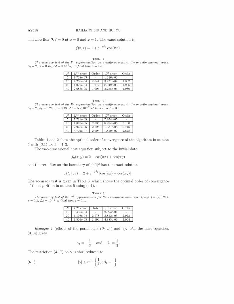
and zero flux !xf = 0 at x = 0 and x = 1. The exact solution is
f(t, x) = 1 + e#'2t cos('x).
Table 1The accuracy test of the P 1 approximation on a uniform mesh in the one-dimensional space.
!0 = 2, " = 0.75, "t = 0.5h2#0 at final time t = 0.5.
N L# error Order L2 error Order5 1.738e-03 - 1.236e-03 -10 4.206e-04 2.047 3.471e-04 1.83220 1.072e-04 1.972 8.949e-05 1.95640 2.688e-05 1.995 2.255e-05 1.989
Table 2The accuracy test of the P 2 approximation on a uniform mesh in the one-dimensional space.
!0 = 2, !1 = 0.25, " = 0.33, "t = 5! 10"7 at final time t = 0.5.
N L# error Order L2 error Order5 7.719e-05 - 7.974e-05 -10 1.820e-05 2.085 8.924e-06 3.16020 2.948e-06 2.626 1.331e-06 2.74640 3.704e-07 2.993 1.810e-07 2.878
Tables 1 and 2 show the optimal order of convergence of the algorithm in section5 with (3.1) for k = 1, 2.
The two-dimensional heat equation subject to the initial data
f0(x, y) = 2 + cos('x) + cos('y)
and the zero flux on the boundary of [0, 1]2 has the exact solution
f(t, x, y) = 2 + e#'2t [cos('x) + cos('y)] .
The accuracy test is given in Table 3, which shows the optimal order of convergenceof the algorithm in section 5 using (4.1).
Table 3The accuracy test of the P 2 approximation for the two-dimensional case. (!0,!1) = (2, 0.25),
" = 0.3, "t = 10"6 at final time t = 0.1.
N L# error Order L2 error Order10 9.435e-04 - 2.993e-04 -20 1.198e-04 2.978 3.812e-05 2.97340 1.503e-05 2.994 4.885e-06 2.964
Example 2 (e"ects of the parameters ("0,"1) and *). For the heat equation,(3.14) gives
aj = (1
3and bj =
1
3.
The restriction (3.17) on * is thus reduced to
(6.1) |*| + min
A1
3, 8"1 ( 1
B.
MAXIMUM-PRINCIPLE-SATISFYING DG SCHEMES A2319
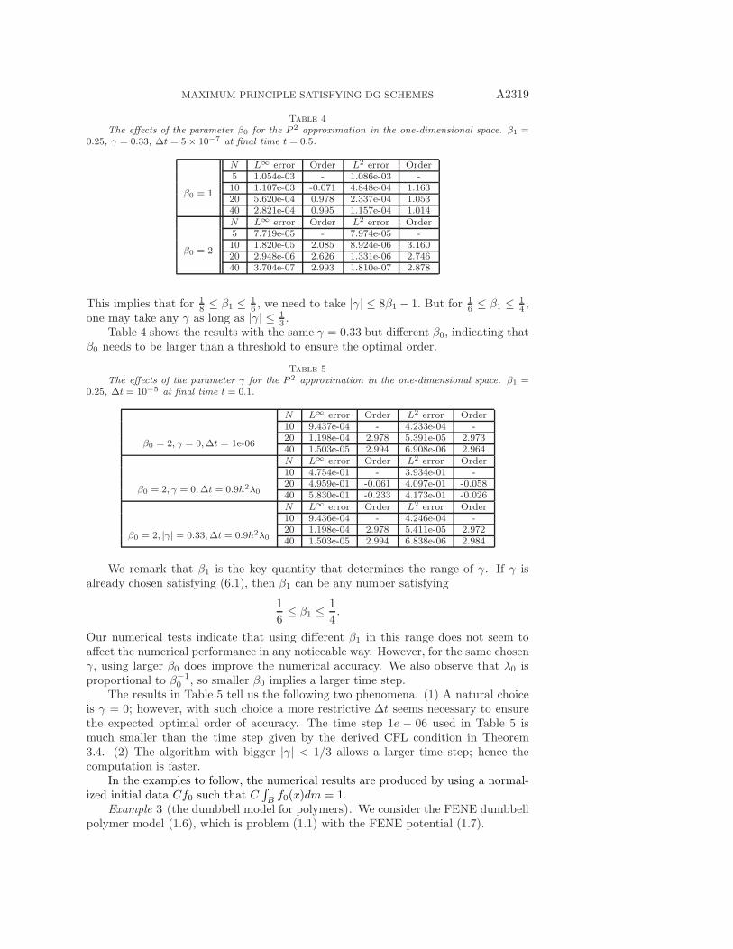
Table 4The e!ects of the parameter !0 for the P 2 approximation in the one-dimensional space. !1 =
0.25, " = 0.33, "t = 5! 10"7 at final time t = 0.5.
!0 = 1
N L# error Order L2 error Order5 1.054e-03 - 1.086e-03 -10 1.107e-03 -0.071 4.848e-04 1.16320 5.620e-04 0.978 2.337e-04 1.05340 2.821e-04 0.995 1.157e-04 1.014
!0 = 2
N L# error Order L2 error Order5 7.719e-05 - 7.974e-05 -10 1.820e-05 2.085 8.924e-06 3.16020 2.948e-06 2.626 1.331e-06 2.74640 3.704e-07 2.993 1.810e-07 2.878
This implies that for 18 + "1 + 1
6 , we need to take |*| + 8"1 ( 1. But for 16 + "1 + 1
4 ,one may take any * as long as |*| + 1
3 .Table 4 shows the results with the same * = 0.33 but di"erent "0, indicating that
"0 needs to be larger than a threshold to ensure the optimal order.
Table 5The e!ects of the parameter " for the P 2 approximation in the one-dimensional space. !1 =
0.25, "t = 10"5 at final time t = 0.1.
!0 = 2, " = 0,"t = 1e-06
N L# error Order L2 error Order10 9.437e-04 - 4.233e-04 -20 1.198e-04 2.978 5.391e-05 2.97340 1.503e-05 2.994 6.908e-06 2.964
!0 = 2, " = 0,"t = 0.9h2#0
N L# error Order L2 error Order10 4.754e-01 - 3.934e-01 -20 4.959e-01 -0.061 4.097e-01 -0.05840 5.830e-01 -0.233 4.173e-01 -0.026
!0 = 2, |"| = 0.33,"t = 0.9h2#0
N L# error Order L2 error Order10 9.436e-04 - 4.246e-04 -20 1.198e-04 2.978 5.411e-05 2.97240 1.503e-05 2.994 6.838e-06 2.984
We remark that "1 is the key quantity that determines the range of *. If * isalready chosen satisfying (6.1), then "1 can be any number satisfying
1
6+ "1 + 1
4.
Our numerical tests indicate that using di"erent "1 in this range does not seem toa"ect the numerical performance in any noticeable way. However, for the same chosen*, using larger "0 does improve the numerical accuracy. We also observe that )0 isproportional to "#1
0 , so smaller "0 implies a larger time step.The results in Table 5 tell us the following two phenomena. (1) A natural choice
is * = 0; however, with such choice a more restrictive #t seems necessary to ensurethe expected optimal order of accuracy. The time step 1e ( 06 used in Table 5 ismuch smaller than the time step given by the derived CFL condition in Theorem3.4. (2) The algorithm with bigger |*| < 1/3 allows a larger time step; hence thecomputation is faster.
In the examples to follow, the numerical results are produced by using a normal-ized initial data Cf0 such that C
+B f0(x)dm = 1.
Example 3 (the dumbbell model for polymers). We consider the FENE dumbbellpolymer model (1.6), which is problem (1.1) with the FENE potential (1.7).
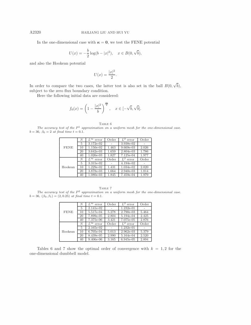
A2320 HAILIANG LIU AND HUI YU
In the one-dimensional case with " = 0, we test the FENE potential
U(x) = ( b
2log(b( |x|2), x " B(0,
)b),
and also the Hookean potential
U(x) =|x|2
2.
In order to compare the two cases, the latter test is also set in the ball B(0,)b),
subject to the zero flux boundary condition.Here the following initial data are considered:
f0(x) =
(1( |x|2
b
) 3b4
, x " [()b,)b].
Table 6The accuracy test of the P 1 approximation on a uniform mesh for the one-dimensional case.
b = 36, !0 = 2 at final time t = 0.1.
FENE
N L# error Order L2 error Order5 3.172e-02 - 3.938e-02 -10 1.150e-02 1.463 9.669e-03 2.02620 3.642e-03 1.659 2.804e-03 1.78640 1.026e-03 1.827 7.125e-04 1.977
Hookean
N L# error Order L2 error Order5 3.315e-02 - 4.194e-02 -10 1.229e-02 1.431 1.034e-02 2.02020 3.878e-03 1.664 2.940e-03 1.81440 1.080e-03 1.845 7.459e-04 1.979
Table 7The accuracy test of the P 2 approximation on a uniform mesh for the one-dimensional case.
b = 36, (!0,!1) = (2, 0.25) at final time t = 0.1.
FENE
N L# error Order L2 error Order5 2.141e-02 - 1.232e-01 -10 5.517e-04 5.278 2.790e-03 5.46420 7.899e-05 2.804 5.194e-04 2.42540 7.375e-06 3.421 7.075e-05 2.876
Hookean
N L# error Order L2 error Order5 2.165e-02 - 1.232e-01 -10 6.705e-04 5.013 2.962e-03 5.37920 8.439e-05 2.990 5.164e-04 2.52040 9.406e-06 3.165 6.945e-05 2.894
Tables 6 and 7 show the optimal order of convergence with k = 1, 2 for theone-dimensional dumbbell model.
MAXIMUM-PRINCIPLE-SATISFYING DG SCHEMES A2321
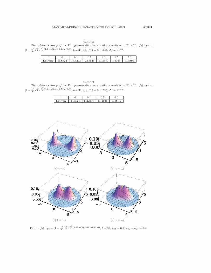
Table 8The relative entropy of the P 2 approximation on a uniform mesh N = 20 ! 20. f0(x, y) =
(1" x2
b )3b4 e
x2
b (1.1 cos(2y)+0.2 sin(2y)), b = 36, (!0,!1) = (4, 0.25), "t = 10"5.
t 0 0.1 0.5 1.0 1.5 2.0Entropy 56.6722 17.5203 2.86945 1.43649 1.1369 1.05801
Table 9The relative entropy of the P 2 approximation on a uniform mesh N = 20 ! 20. f0(x, y) =
(1" x2
b )3b4 e
x2
b (0.2 cos(2y)"0.7 sin(2y)), b = 36, (!0,!1) = (4, 0.25), "t = 10"5.
t 0 0.1 0.5 0.6Entropy 43.3521 6.37854 1.12631 1.02612
(a) t = 0 (b) t = 0.5
(c) t = 1.0 (d) t = 2.0
Fig. 1. f0(x, y) = (1" x2
b)3b4 e
x2
b (1.1 cos(2y)+0.2 sin(2y)), b = 36, $11 = 0.3, $12 = $21 = 0.2.
A2322 HAILIANG LIU AND HUI YU
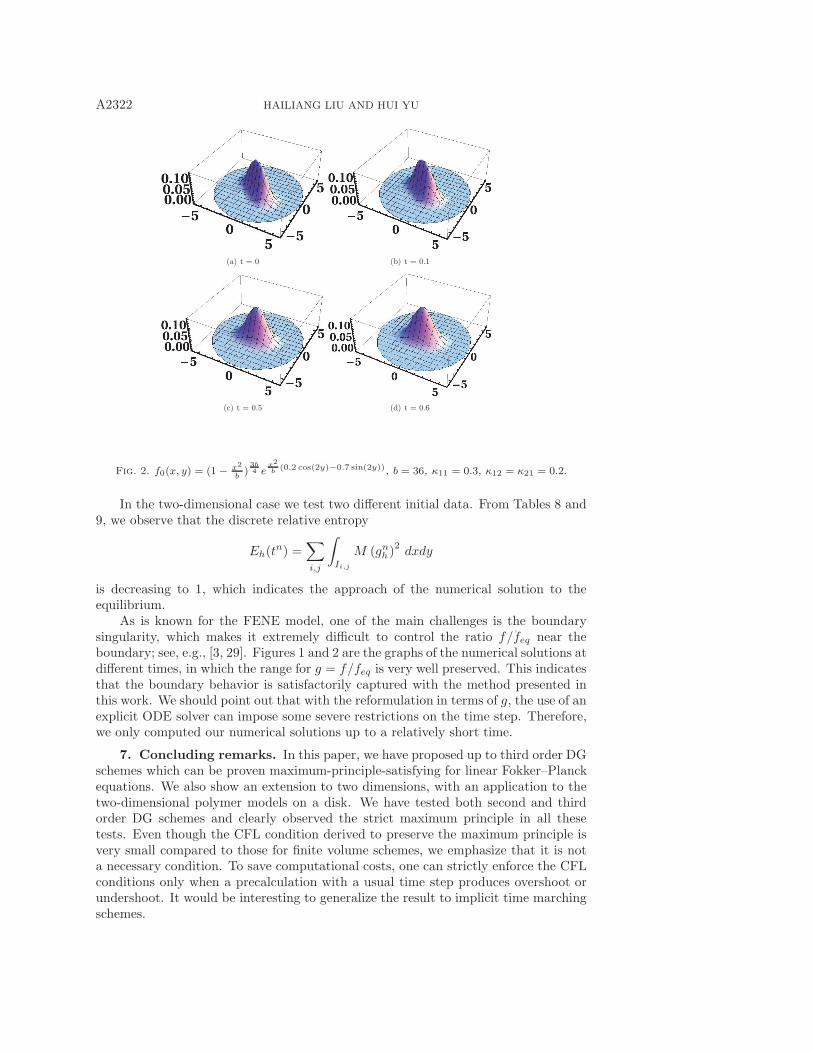
(a) t = 0 (b) t = 0.1
(c) t = 0.5 (d) t = 0.6
,
Fig. 2. f0(x, y) = (1 " x2
b )3b4 e
x2
b (0.2 cos(2y)"0.7 sin(2y)), b = 36, $11 = 0.3, $12 = $21 = 0.2.
In the two-dimensional case we test two di"erent initial data. From Tables 8 and9, we observe that the discrete relative entropy
Eh(tn) =
1
i,j
$
Ii,j
M (gnh)2 dxdy
is decreasing to 1, which indicates the approach of the numerical solution to theequilibrium.
As is known for the FENE model, one of the main challenges is the boundarysingularity, which makes it extremely di!cult to control the ratio f/feq near theboundary; see, e.g., [3, 29]. Figures 1 and 2 are the graphs of the numerical solutions atdi"erent times, in which the range for g = f/feq is very well preserved. This indicatesthat the boundary behavior is satisfactorily captured with the method presented inthis work. We should point out that with the reformulation in terms of g, the use of anexplicit ODE solver can impose some severe restrictions on the time step. Therefore,we only computed our numerical solutions up to a relatively short time.
7. Concluding remarks. In this paper, we have proposed up to third order DGschemes which can be proven maximum-principle-satisfying for linear Fokker–Planckequations. We also show an extension to two dimensions, with an application to thetwo-dimensional polymer models on a disk. We have tested both second and thirdorder DG schemes and clearly observed the strict maximum principle in all thesetests. Even though the CFL condition derived to preserve the maximum principle isvery small compared to those for finite volume schemes, we emphasize that it is nota necessary condition. To save computational costs, one can strictly enforce the CFLconditions only when a precalculation with a usual time step produces overshoot orundershoot. It would be interesting to generalize the result to implicit time marchingschemes.
MAXIMUM-PRINCIPLE-SATISFYING DG SCHEMES A2323
REFERENCES
[1] D. N. Arnold, An interior penalty finite element method with discontinuous elements, SIAMJ. Numer. Anal., 19 (1982), pp. 742–760.
[2] D. N. Arnold, F. Brezzi, B. Cockburn, and L. D. Marini, Unified analysis of discontinuousGalerkin methods for elliptic problems, SIAM J. Numer. Anal., 39 (2002), pp. 1749–1779.
[3] A. Arnold, J. A. Carrillo, and C. Manzini, Refined long-time asymptotics for some poly-meric fluid flow models, Commun. Math. Sci., 8 (2010), pp. 763–782.
[4] G. A. Baker, Finite element methods for elliptic equations using nonconforming elements,Math. Comp., 31 (1977), pp. 45–59.
[5] F. Bassi and S. Rebay, A high-order accurate discontinuous finite element method for thenumerical solution of the compressible Navier-Stokes equations, J. Comput. Phys., 131(1997), pp. 267–279.
[6] C. E. Baumann and J. T. Oden, A discontinuous hp finite element method for convection-di!usion problems, Comput. Methods Appl. Mech. Engrg., 175 (1999), pp. 311–341.
[7] Yu. A. Berezin, V. N. Khudick, and M. S. Pekker, Conservative finite di!erence schemesfor the Fokker-Planck equation not violating the law of an increasing entropy, J. Comput.Phys., 69 (1987), pp. 163–174.
[8] M. Bessemoulin-Chatard and F. Filbet, A finite volume scheme for nonlinear degenerateparabolic equations, SIAM J. Sci. Comput., 34 (2012), pp. B559–B583.
[9] P. Degond, C. Buet, S. Cordier, and M. Lemou, Fast algorithms for numerical, conserva-tive, and entropy approximations of the Fokker-Planck equation, J. Comput. Phys., 133(1997), pp. 310–322.
[10] P. Castillo, B. Cockburn, I. Perugia, and D. Schotzau, An a priori error analysis ofthe local discontinuous Galerkin method for elliptic problems, SIAM J. Numer. Anal., 38(2000), pp. 1676–1706.
[11] J. S. Chang and G. Cooper, A practical di!erence scheme for Fokker-Planck equations, J.Comput. Phys., 6 (1970), pp. 1–16.
[12] C. Chauviere and A. Lozinski, Simulation of complex viscoelastic flows using Fokker-Planckequation: 3D FENE model, J. Non-Newtonian Fluid Mech., 122 (2004), pp. 201–214.
[13] C. Chauviere and A. Lozinski, Simulation of dilute polymer solutions using a Fokker-Planckequation, J. Comput. Fluids, 33 (2004), pp. 687–696.
[14] C. Chauviere and A. Lozinski, A fast solver for Fokker-Planck equation applied to viscoelasticflows calculations: 2D FENE model, J. Comput. Phys., 189 (2003), pp. 607–625.
[15] Y. Cheng and C.-W. Shu, A discontinuous Galerkin finite element method for time dependentpartial di!erential equations with higher order derivatives, Math. Comp., 77 (2007), pp.699–730.
[16] B. Cockburn, S. Hou, and C.-W. Shu, The Runge-Kutta local projection discontinuousGalerkin finite element method for conservation laws. IV. The multidimensional case,Math. Comp., 54 (1990), pp. 545–581.
[17] B. Cockburn, S. Y. Lin, and C.-W. Shu, TVB Runge-Kutta local projection discontinuousGalerkin finite element method for conservation laws. III. One-dimensional systems, J.Comput. Phys., 84 (1989), pp. 90–113.
[18] B. Cockburn and C.-W. Shu, TVB Runge-Kutta local projection discontinuous Galerkin finiteelement method for conservation laws. II. General framework, Math. Comp., 52 (1989),pp. 411–435.
[19] B. Cockburn and C.-W. Shu, The Runge-Kutta discontinuous Galerkin method for conser-vation laws. V. Multidimensional systems, J. Comput. Phys., 141 (1998), pp. 199–224.
[20] B. Cockburn and C.-W. Shu, The local discontinuous Galerkin method for time-dependentconvection-di!usion systems, SIAM J. Numer. Anal., 35 (1998), pp. 2440–2463.
[21] B. Cockburn and C. Dawson, Some extensions of the local discontinuous Galerkin methodfor convection-di!usion equations in multidimensions, in Proceedings of the Conferenceon the Mathematics of Finite Elements and Applications, MAFELAP X, J. R. Whiteman,ed., Elsevier, New York., 2000, pp. 225–238.
[22] B. Cockburn, G. Kanschat, I. Perugia, and D. Schotzau, Superconvergence of the localdiscontinuous Galerkin method for elliptic problems on Cartesian grids, SIAM J. Numer.Anal., 39 (2001), pp. 264–285.
[23] P. Degond and B. Lucquin-Desreux, An entropy scheme for the Fokker–Planck collisionoperator of plasma kinetic theory, Numer. Math., 68 (1994), pp. 239–262.
[24] G. C. Pomraning, E. W. Larsen, C. D. Levermore, and J. G. Sanderson, Discretizationmethods for one dimensional Fokker–Planck operators, J. Comput. Phys., 61 (1985), pp.359–390.
A2324 HAILIANG LIU AND HUI YU
[25] E. M. Epperlein, Implicit and conservative di!erence schemes for the Fokker–Planck equation,J. Comput. Phys., 112 (1994), pp. 291–297.
[26] A. D. Fokker, Die mittlere energie rotierender elektrischer dipole im strahlungsfeld, Ann.Phys., 348 (1914), pp. 810–820.
[27] G. Gassner, F. Lorcher, and C.-D. Munz, A contribution to the construction of di!usionfluxes for finite volume and discontinuous Galerkin schemes, J. Comput. Phys., 224 (2007),pp. 1049–1063.
[28] J. S. Hesthaven and T. Warburton, Nodal Discontinuous Galerkin Methods: Algorithms,Analysis, and Applications, Springer, New York, 2007.
[29] B. Jourdain, T. Lelievre, C. Le Bris, and F. Otto, Long-time asymptotics of a multiscalemodel for polymeric fluid flows, Arch. Ration. Mech. Anal., 181 (2006), pp. 97–148.
[30] L. P. Kadanoff, Statistical Physics: Statics, Dynamics and Renormalization, World Scientific,New York, 2000.
[31] D. J. Knezevic and E. Suli, Spectral Galerkin approximation of Fokker-Planck equations withunbounded drift, M2AN Math. Model. Numer. Anal., 43 (2009), pp. 445–485.
[32] R. S. Langley, A finite element method for the statistics of nonlinear random vibration, J.Sound Vibr., 101 (1985), pp. 41–54.
[33] H. P. Langtangeh, A general numerical solution method for Fokker–Planck equations withapplications to structural reliability, Probab. Eng. Mech., 6 (1991), pp. 33–48.
[34] B. Q. Li, Discontinuous Finite Elements in Fluid Dynamics and Heat Transfer, ComputationalFluid and Solid Mechanics, Springer, London, 2006.
[35] C. Liu and H. Liu, Boundary conditions for the microscopic FENE models, SIAM J. Appl.Math., 68 (2008), pp. 1304–1315.
[36] H. Liu and J. Yan, The direct discontinuous Galerkin (DDG) methods for di!usion problems,SIAM J. Numer. Anal., 47 (2009), pp. 675–698.
[37] H. Liu and J. Shin, The Cauchy–Dirichlet problem for the finitely extensible nonlinear elasticdumbbell model of polymeric fluids, SIAM J. Math. Anal., 44 (2012), pp. 3617–3648.
[38] H. Liu and J. Yan, The direct discontinuous Galerkin (DDG) method for di!usion with in-terface corrections, Commun. Comput. Phys., 8 (2010), pp. 541–564.
[39] H. Liu and H. Yu, An entropy satisfying conservative method for the Fokker–Planck equationof the finitely extensible nonlinear elastic dumbbell model, SIAM J. Numer. Anal., 50(2012), pp. 1207–1239.
[40] H. Liu and H. Yu, The entropy satisfying dicontinuous Galerkin method for Fokker-PlanckEquations, J. Sci. Comput., to appear; DOI 10.1007/s10915-014-9878-1.
[41] H. Liu, Optimal error estimates of the direct discontinuous Galerkin method for convection-di!usion equations, Math. Comp, to appear.
[42] X.-D. Liu and S. Osher, Nonoscillatory high order accurate self-similar maximum principlesatisfying shock capturing schemes I, SIAM J. Numer. Anal., 33 (1996), pp. 760–779.
[43] J. T. Oden, I. Babuska, and C. E. Baumann, A discontinuous hp finite element method fordi!usion problems, J. Comput. Phys., 146 (1998), pp. 491–519.
[44] B. Perthame, Transport Equations in Biology, Frontiers in Mathematics, Birkhauser Verlag,Basel, 2007.
[45] M. Planck, Sitzber. Preuss. Akad. Wiss., 1917, p. 324.[46] W. H. Reed and T. R. Hill, Triangular Mesh Methods for the Neutron Transport Equation,
Tech. Report LA-UR-73-479, Los Alamos Scientific Laboratory, Los Alamos, NM, 1973.[47] H. Risken, The Fokker-Planck Equation: Methods of Solution and Applications, 2nd ed.,
Springer Ser. Synergetics 18, Springer-Verlag, Berlin, 1989.[48] B. Riviere, Discontinuous Galerkin Methods for Solving Elliptic and Parabolic Equations:
Theory and Implementation, SIAM, Philadelphia, 2008.[49] J. Shen and H. Yu, On the approximation of the Fokker–Planck equation of the finitely ex-
tensible nonlinear elastic dumbbell model I: A new weighted formulation and an optimalspectral-Galerkin algorithm in two dimensions, SIAM J. Numer. Anal., 50 (2012), pp.1136–1161.
[50] C.-W. Shu, Discontinuous Galerkin methods: General approach and stability, in NumericalSolutions of Partial Di!erential Equations, S. Bertoluzza, S. Falletta, G. Russo, and C.-W.Shu, eds., Advanced Courses in Mathematics, CRM Barcelona, Birkhauser, Basel, 2009,pp. 149–201.
[51] B. F. Spencer, Jr., and L. A. Bergman, On the numerical solution of the Fokker-Planckequations for nonlinear stochastic systems, Nonlinear Dynam., 4 (1993), pp. 357–372.
[52] B. van Leer and S. Nomura, Discontinuous Galerkin for di!usion, in Proceedings of the 17thAIAA Computational Fluid Dynamics Conference, AIAA, Reston, VA, 2005, AIAA-2005-5108.
MAXIMUM-PRINCIPLE-SATISFYING DG SCHEMES A2325
[53] H. R. Warner, Kinetic theory and rheology of dilute suspensions of finitely extendible dumb-bells, Ind. Eng. Chem. Fundamen., 11 (1972), pp. 379–387.
[54] M. F. Wheeler, An elliptic collocation-finite element method with interior penalties, SIAM J.Numer. Anal., 15 (1978), pp. 152–161.
[55] X. Zhang, Y. Liu, and C.-W. Shu, Maximum-principle-satisfying high order finite volumeweighted essentially nonoscillatory schemes for convection-di!usion equations, SIAM J.Sci. Comput., 34 (2012), pp. A627–A658.
[56] X.-X. Zhang and C.-W. Shu, On maximum-principle-satisfying high order schemes for scalarconservation laws, J. Comput. Phys., 229 (2010), pp. 3091–3120.
[57] Y.-F. Zhang, X.-X. Zhang, and C.-W. Shu, Maximum-principle-satisfying second order dis-continuous Galerkin schemes for convection-di!usion equations on triangular meshes, J.Comput. Phys., 234 (2013), pp. 295–316.