Parallel Discontinuous Galerkin Method

ParallelDiscontinuous Galerkin Method

Yin Ki, NG

The Chinese University of Hong Kong

Aug 5, 2015

Mentors: Dr. Ohannes Karakashian, Dr. Kwai Wong

•Project Goal

• Implement parallelization on Discontinuous Galerkin Method (DG-FEM)

• scaled on existing supercomputers

Overview

•Overview

•Mathematics behind

•1D Parallelization

•Future Work

•Acknowledgement

Discontinuous Galerkin Method (DG-FEM)

• Discontinuous Galerkin Method (DG-FEM)

– A class of Finite Element Method (FEM)

– Finding approximate solutions to system of differential equations

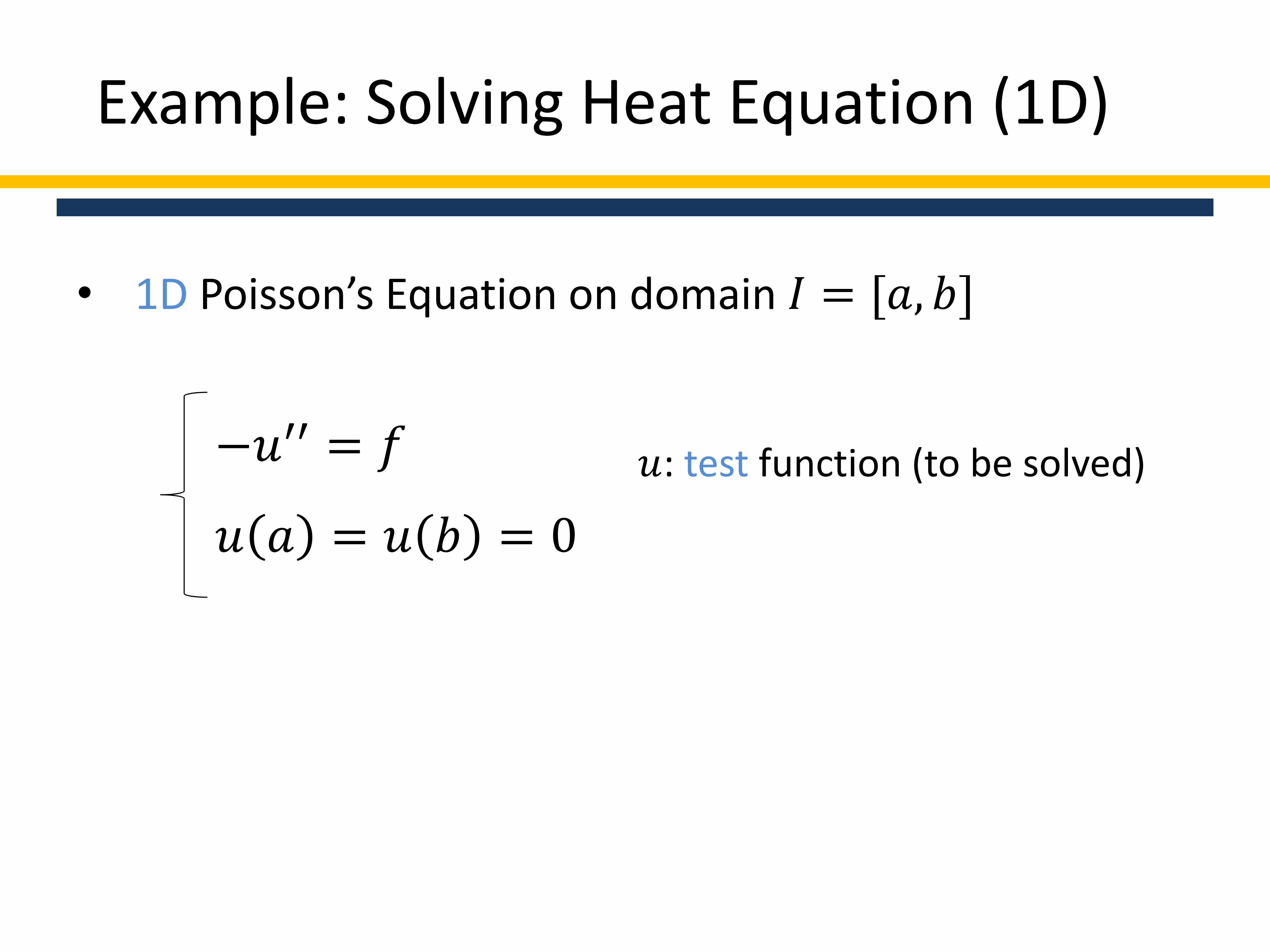
Example: Solving Heat Equation (1D)

• 1D Poisson’s Equation on domain 𝐼 = [𝑎, 𝑏]

−𝑢′′ = 𝑓

𝑢 𝑎 = 𝑢 𝑏 = 0

𝑢: test function (to be solved)

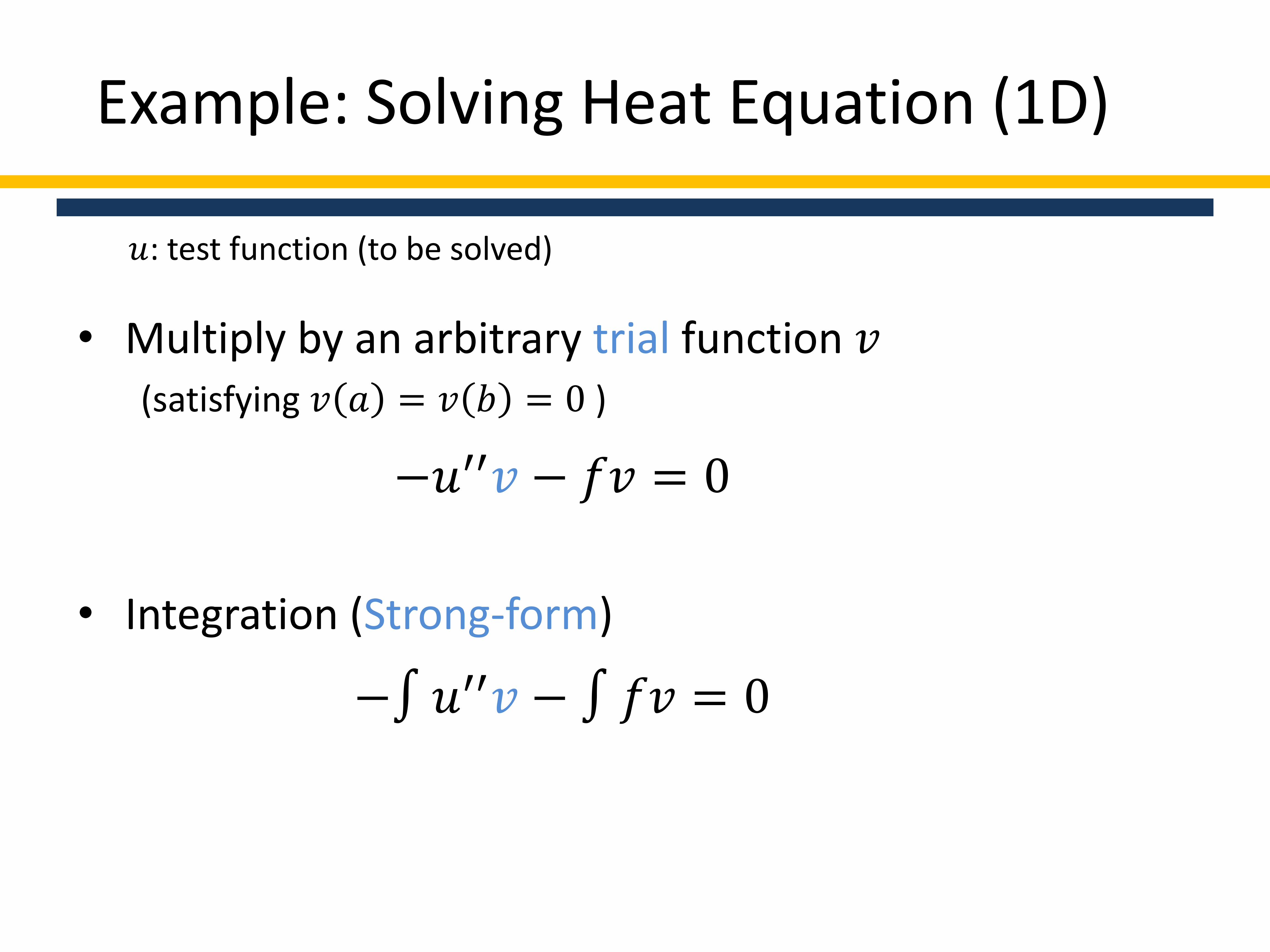
Example: Solving Heat Equation (1D)

• Multiply by an arbitrary trial function 𝑣(satisfying 𝑣 𝑎 = 𝑣 𝑏 = 0 )

• Integration (Strong-form)

−𝑢′′𝑣 − 𝑓𝑣 = 0

−∫ 𝑢′′𝑣 − ∫ 𝑓𝑣 = 0

𝑢: test function (to be solved)

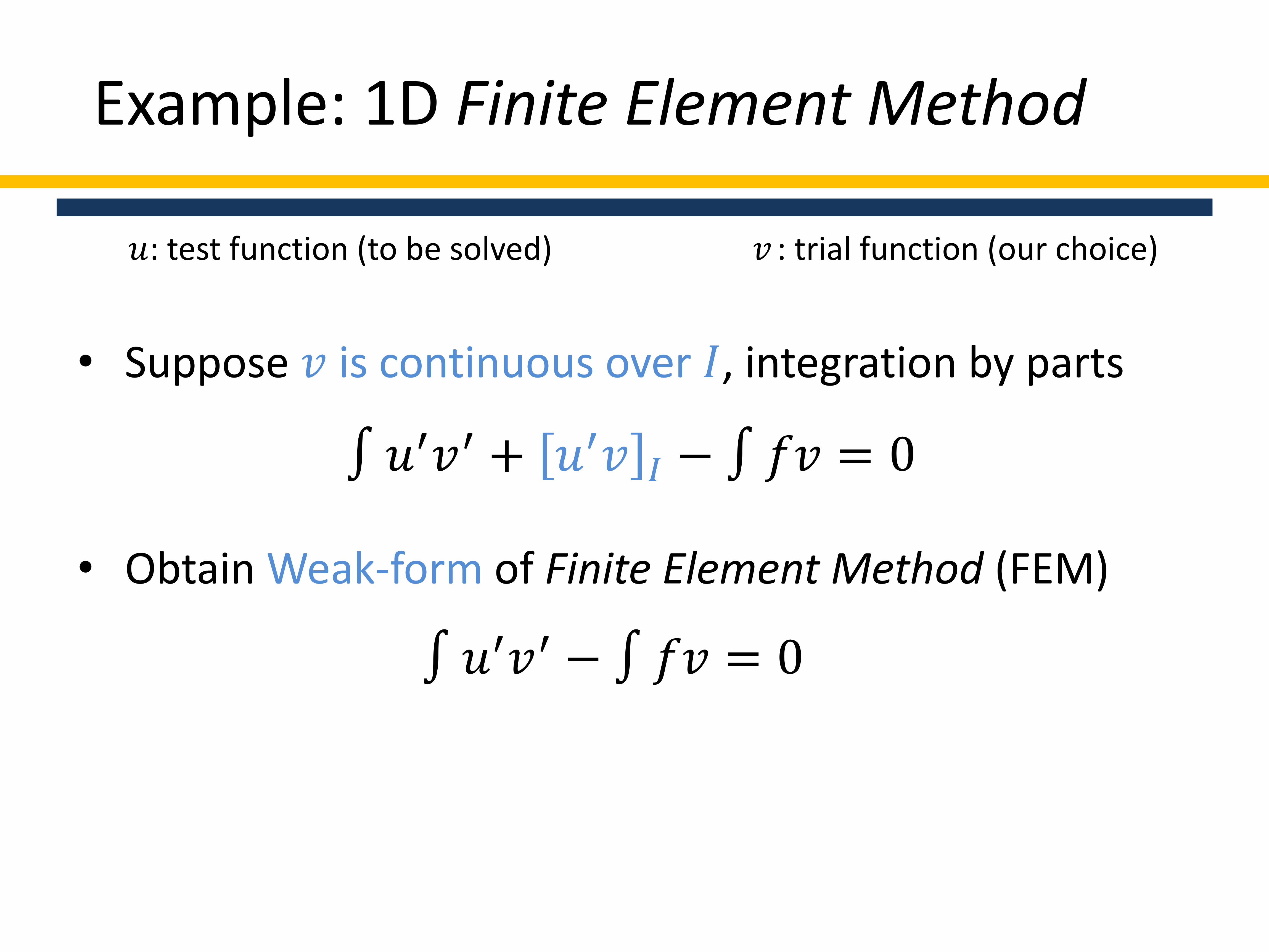
• Suppose 𝑣 is continuous over 𝐼, integration by parts

• Obtain Weak-form of Finite Element Method (FEM)

Example: 1D Finite Element Method

𝑢: test function (to be solved) 𝑣 : trial function (our choice)

∫ 𝑢′𝑣′ + 𝑢′𝑣 𝐼 − ∫ 𝑓𝑣 = 0

∫ 𝑢′𝑣′ − ∫ 𝑓𝑣 = 0

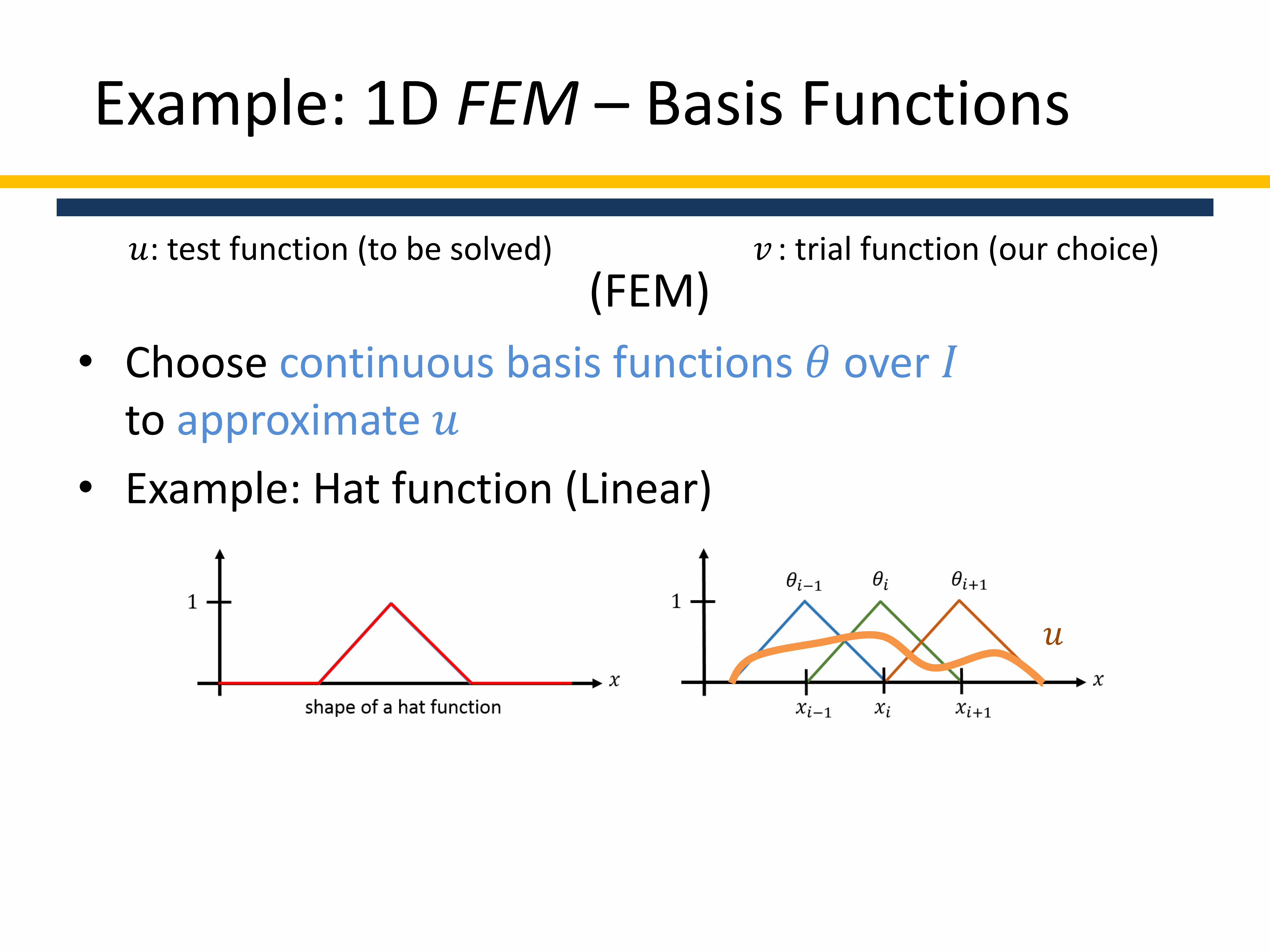
• Choose continuous basis functions 𝜃 over 𝐼to approximate 𝑢

• Example: Hat function (Linear)


𝑢

Example: 1D FEM – Basis Functions

(FEM)

• Choose 𝑣 to be the the basis functions 𝜃

• Approximate 𝑢i = 𝑗 𝑢𝑗 𝑣𝑗 : linear combination of 𝑣𝑗

𝐼

𝑣0′𝑣0′

𝐼

𝑣1′𝑣0′

𝐼

𝑣2′𝑣0

′

𝐼

𝑣0′𝑣1′

𝐼

𝑣1′𝑣1′

𝐼

𝑣2′𝑣1′

𝐼

𝑣0′𝑣2′

𝐼

𝑣1′𝑣2′

𝐼

𝑣2′𝑣2′

𝑢0

𝑢1

𝑢2

𝐼

𝑓𝑣0

𝐼

𝑓𝑣1

𝐼

𝑓𝑣2

− = 0


(FEM)

∫ 𝑢′𝑣′ − ∫ 𝑓𝑣 = 0

Example: 1D FEM – Basis Functions

• Suppose 𝑣 is discontinuous on 𝑥𝑗

• Integration by parts on each interval

𝑣(𝐼0)

𝑥0 𝑥1 𝑥2 𝑥3

𝑣(𝐼1)

𝑣(𝐼2)

+ −

+ −

+−

−∫ 𝑢′′𝑣 = − 𝑗 ∫𝐼𝑗𝑢′′ 𝑣 = 𝑗(∫𝐼𝑗

𝑢′ 𝑣′ ) − 𝑗 𝑢′𝑣 𝑥𝑗

𝑥𝑗+1)

𝑥𝑗+: start of the “left” interval 𝐼𝑗

𝑥𝑗−: start of the “right” interval 𝐼𝑗−1


Example: 1D DG-FEM

−

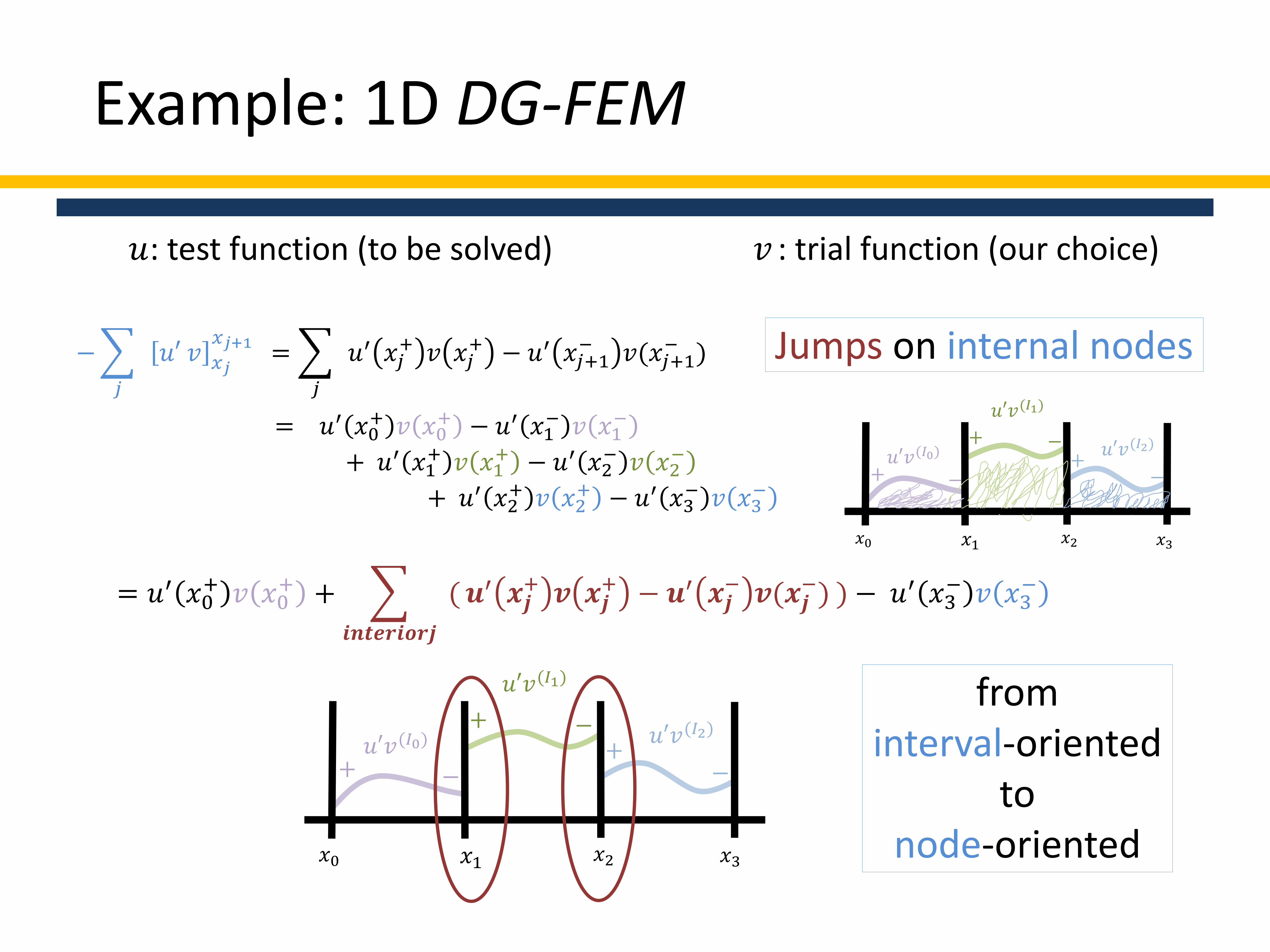
𝑗

𝑢′ 𝑣 𝑥𝑗

𝑥𝑗+1=

𝑗

𝑢′ 𝑥𝑗+ 𝑣 𝑥𝑗

+ − 𝑢′ 𝑥𝑗+1− 𝑣(𝑥𝑗+1

− )

= 𝑢′ 𝑥0+ 𝑣 𝑥0

+ − 𝑢′ 𝑥1− 𝑣 𝑥1

−

+ 𝑢′ 𝑥1+ 𝑣 𝑥1

+ − 𝑢′ 𝑥2− 𝑣 𝑥2

−

+ 𝑢′ 𝑥2+ 𝑣 𝑥2

+ − 𝑢′ 𝑥3− 𝑣 𝑥3

−

= 𝑢′ 𝑥0+ 𝑣 𝑥0

+ +

𝒊𝒏𝒕𝒆𝒓𝒊𝒐𝒓𝒋

( 𝒖′ 𝒙𝒋+ 𝒗 𝒙𝒋

+ − 𝒖′ 𝒙𝒋− 𝒗(𝒙𝒋

−) ) − 𝑢′ 𝑥3− 𝑣 𝑥3

−

𝑢′𝑣(𝐼0)

𝑥0 𝑥1 𝑥2 𝑥3

𝑢′𝑣(𝐼1)

𝑢′𝑣(𝐼2)

+ −

+ −+

−

from interval-oriented

to node-oriented


Jumps on internal nodes

Example: 1D DG-FEM

𝑢′𝑣(𝐼0)

𝑥0 𝑥1 𝑥2 𝑥3

𝑢′𝑣(𝐼1)

𝑢′𝑣(𝐼2)

+ −

+ −+

−

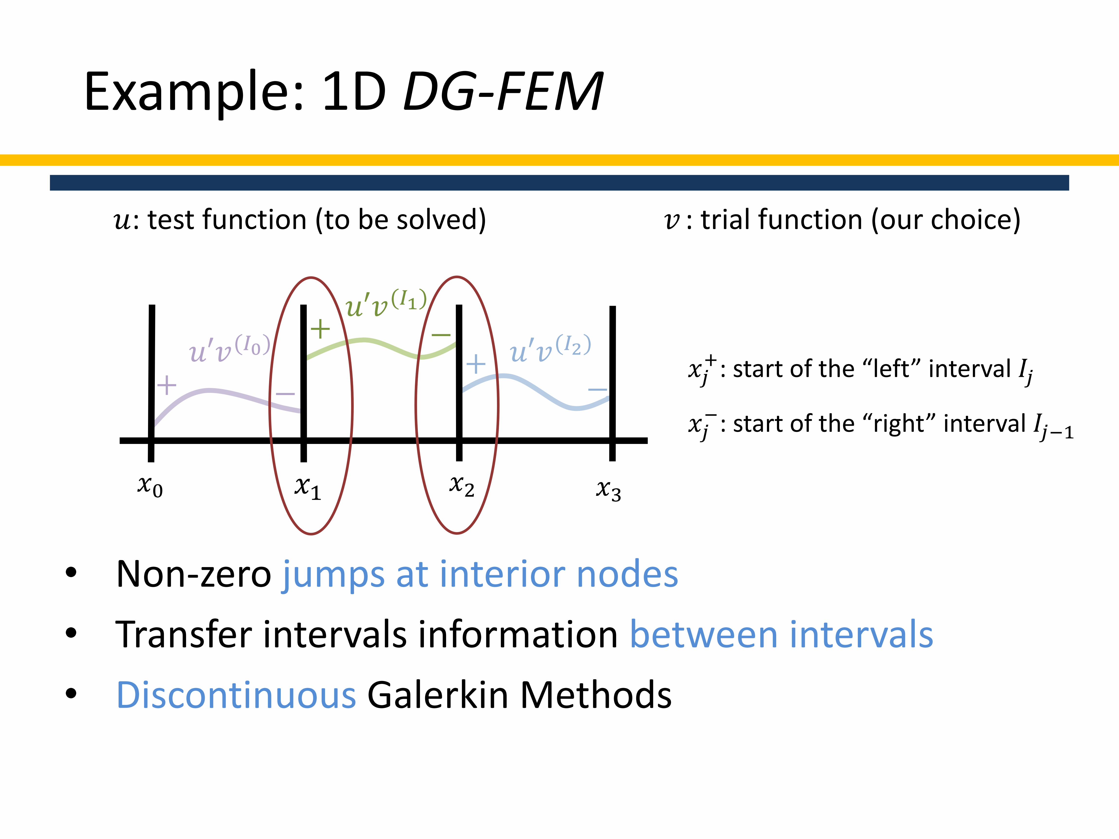
• Non-zero jumps at interior nodes

• Transfer intervals information between intervals

• Discontinuous Galerkin Methods

𝑢′𝑣(𝐼0)

𝑥0 𝑥1 𝑥2 𝑥3

𝑢′𝑣(𝐼1)

𝑢′𝑣(𝐼2)

+ −

+ −+

−𝑥𝑗+: start of the “left” interval 𝐼𝑗


Example: 1D DG-FEM


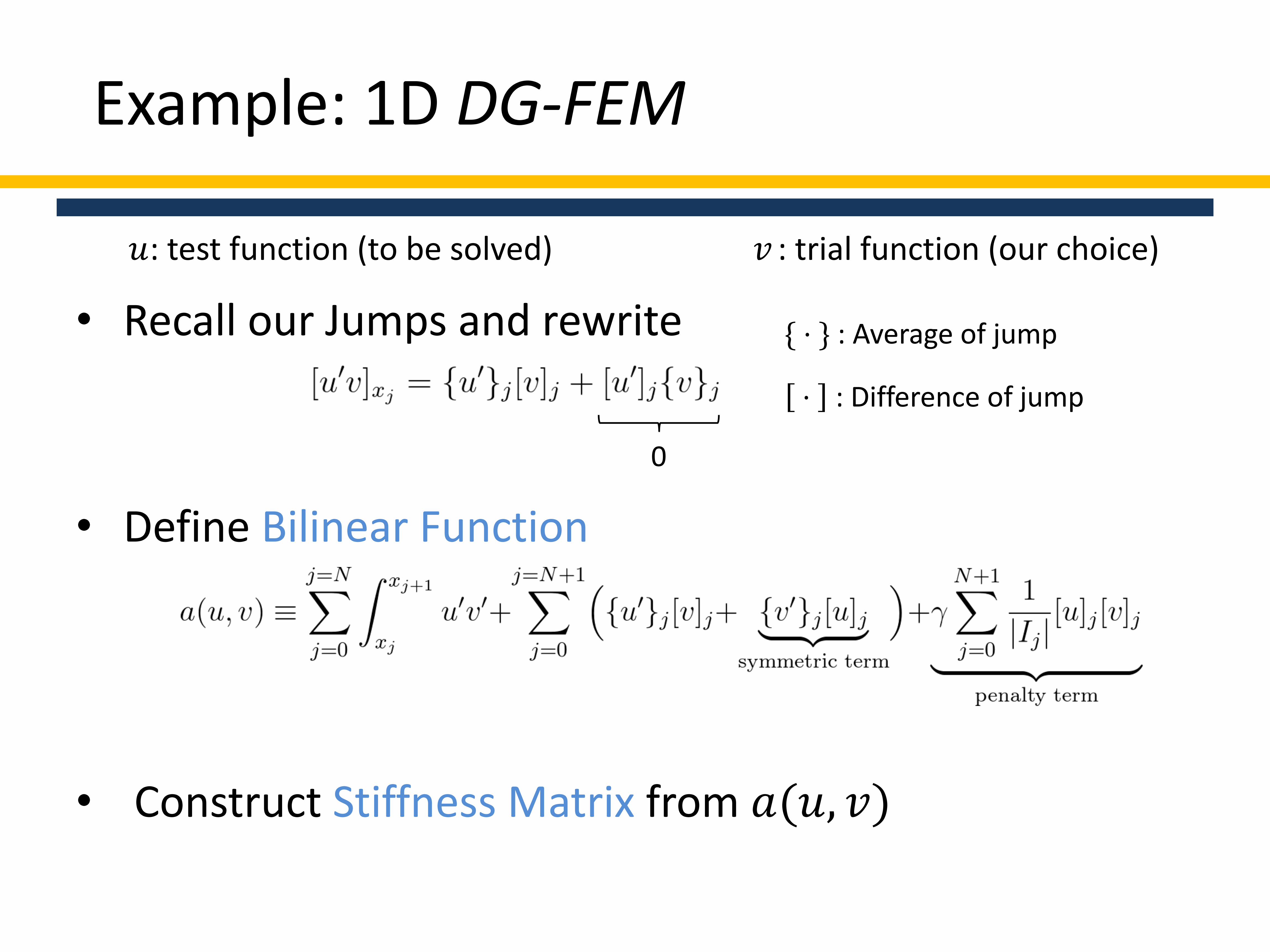
• Recall our Jumps and rewrite

• Define Bilinear Function

• Construct Stiffness Matrix from 𝑎(𝑢, 𝑣)

{ ⋅ } : Average of jump

⋅ : Difference of jump

Example: 1D DG-FEM


0

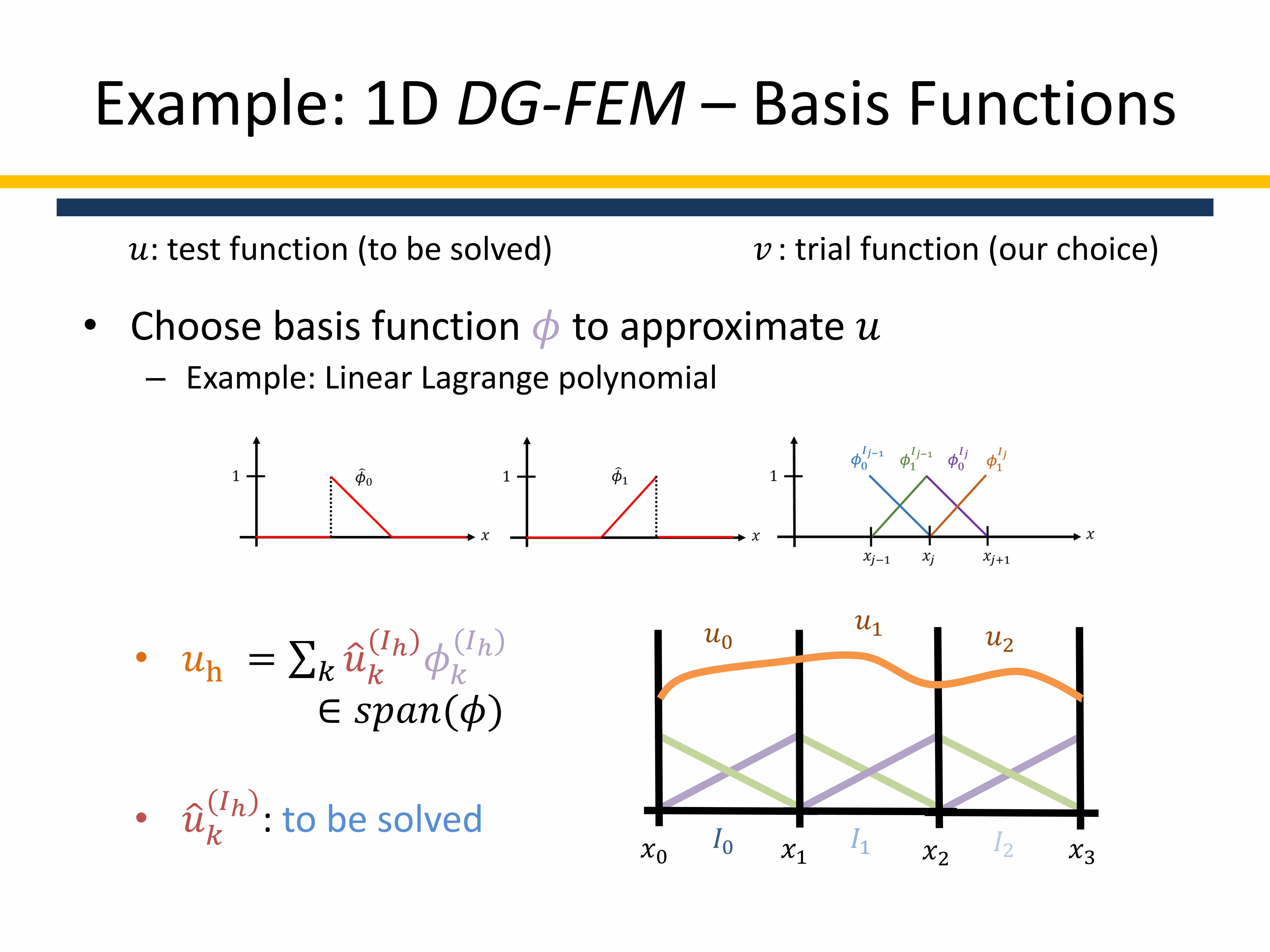
• Choose basis function 𝜙 to approximate 𝑢– Example: Linear Lagrange polynomial

𝑥2𝑥1𝑥0 𝑥3

𝑢0𝑢1

𝐼0 𝐼1 𝐼2

𝑢2• 𝑢h = 𝑘 𝑢𝑘

(𝐼ℎ)𝜙𝑘

(𝐼ℎ)

∈ 𝑠𝑝𝑎𝑛(𝜙)

• 𝑢𝑘(𝐼ℎ)

: to be solved


Example: 1D DG-FEM – Basis Functions

• Also choose 𝑣 to be 𝜙

• Stiffness Matrix from 𝑎 𝑢, 𝑣 => from 𝑎 𝜙 𝑘𝑢, 𝜙 𝑘𝑣

𝑢h = 𝑘 𝑢𝑘(𝐼ℎ)

𝜙𝑘(𝐼ℎ) 𝑣: trial function (our choice) , 𝑢𝑘

(𝐼ℎ)to be solved

Example: 1D DG-FEM – Basis Functions

𝑢 ∈ 𝑠𝑝𝑎𝑛(𝜙) 𝑣 = 𝜙

𝜙0(𝐼0) 𝜙1

(𝐼0) 𝜙0(𝐼1) 𝜙1

(𝐼1) 𝜙0(𝐼2) 𝜙1

(𝐼2)

𝜙0(𝐼0)

𝜙1(𝐼0)

𝜙0(𝐼1)

𝜙1(𝐼1)

𝜙0(𝐼2)

𝜙1(𝐼2)

𝑢0

(𝐼0)

𝑢1

(𝐼0)

𝑢0

(𝐼1)

𝑢1

(𝐼1)

𝑢0

(𝐼2)

𝑢1

(𝐼2)

= ⋯

𝜙0(𝐼0) 𝜙1

(𝐼0) 𝜙0(𝐼1) 𝜙1

(𝐼1) 𝜙0(𝐼2) 𝜙1

(𝐼2)

𝜙0(𝐼0)

𝜙1(𝐼0)

𝜙0(𝐼1)

𝜙1(𝐼1)

𝜙0(𝐼2)

𝜙1(𝐼2)

– Each block contains basis functions interaction w.r.t intervals

– Diagonal blocks: within an interval

– Sub-diagonal blocks: adjacent intervals

– Others: ZEROS (non-adjacent intervals)

Info within Interval 𝐼1



Info across Interval 𝐼0 and 𝐼1

Zeros (Non adjacent intervals)





Example: 1D DG-FEM

“++” “+-” “-+” “--”

𝑥𝑗+: start of the “left” interval 𝐼𝑗


0

𝑢 ∈ 𝑠𝑝𝑎𝑛(𝜙) 𝑣 = 𝜙𝑢h = 𝑘 𝑢𝑘

(𝐼ℎ)𝜙𝑘

(𝐼ℎ) 𝑣: trial function (our choice)

Example: 1D DG-FEM

“++” “+-” “-+” “--”






Example

• 𝑗 = 1 (on 𝑥1)

“--” “+-”

“-+” “++”

𝜙0(𝐼0)

𝜙1(𝐼0)

𝜙0(𝐼1)

𝜙1(𝐼1)

𝜙0(𝐼2)

𝜙1(𝐼2)

Example: 1D DG-FEM

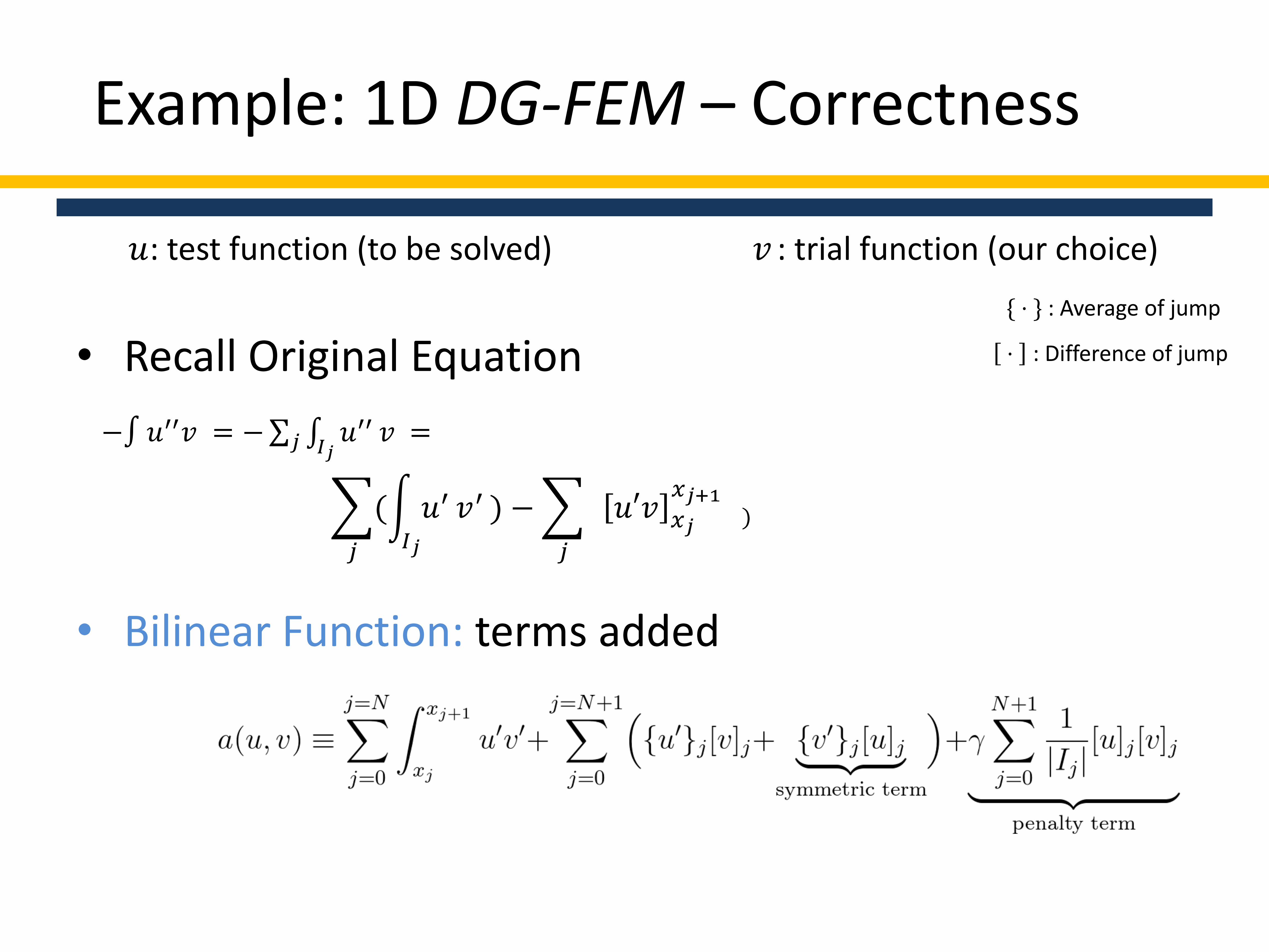
• Recall Original Equation

• Bilinear Function: terms added

{ ⋅ } : Average of jump

⋅ : Difference of jump

Example: 1D DG-FEM – Correctness


−∫ 𝑢′′𝑣 = − 𝑗 ∫𝐼𝑗𝑢′′ 𝑣 =

𝑗

( 𝐼𝑗

𝑢′ 𝑣′ ) −

𝑗

𝑢′𝑣 𝑥𝑗

𝑥𝑗+1)

• Symmetric term– Added for the matrix to be symmetric

• Penalty term– Added for the matrix to be positive-definite



• Show stiffness matrix postive-definite

– Show

• 𝑉ℎ: DG Finite Element Space 𝑢1,ℎ: well-defined norm



• 𝑉ℎ: DG Finite Element Space 𝑢1,ℎ: well-defined norm

• 1. Define

- can be shown well-defined.



Show

• 2. Important Inequalities used– Trace Inequality

– Trace Inequality (1D)

• 𝐻: Length of Interval



Show

𝑎 𝑏𝐻

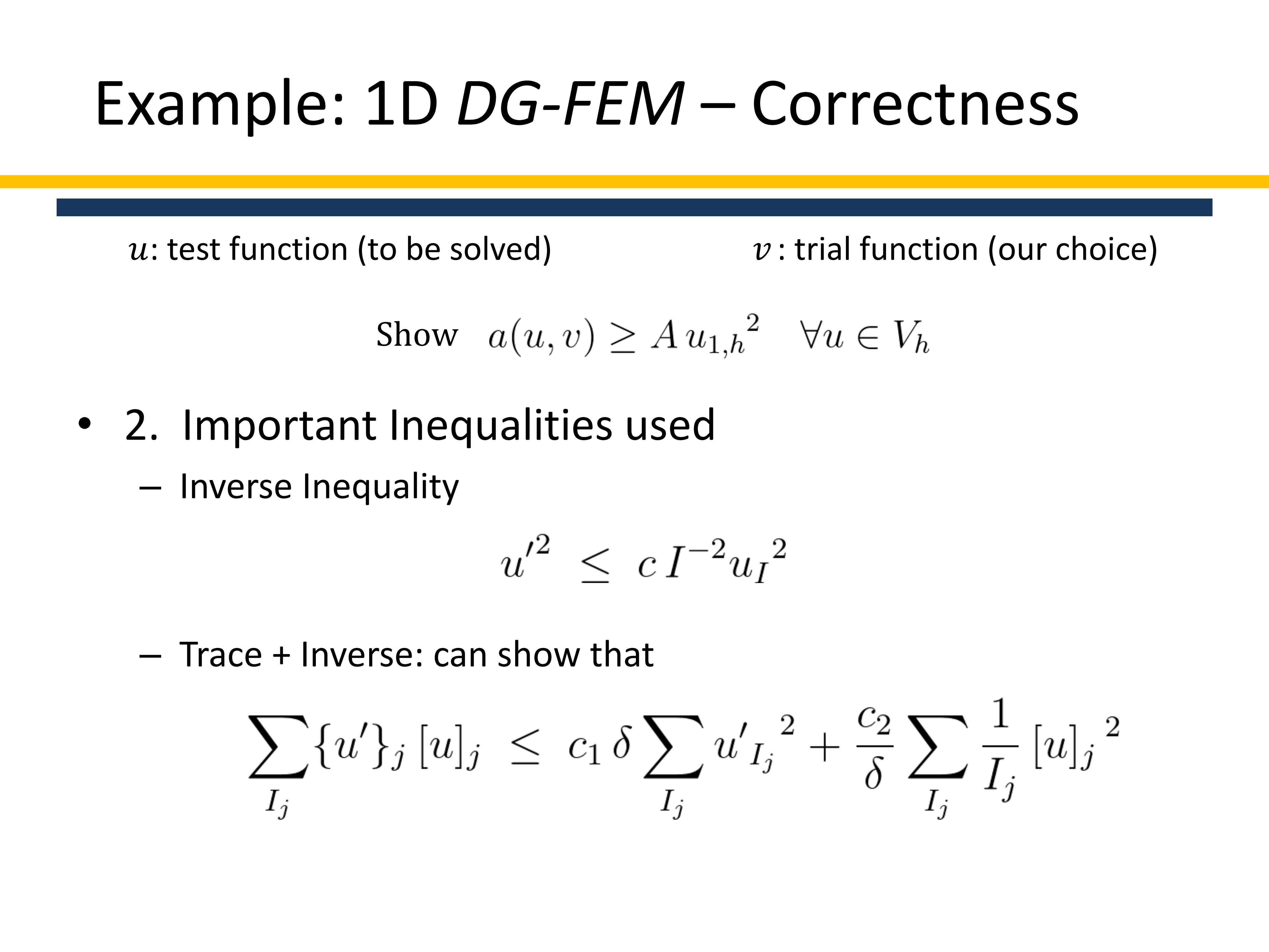
• 2. Important Inequalities used– Inverse Inequality

– Trace + Inverse: can show that



Show

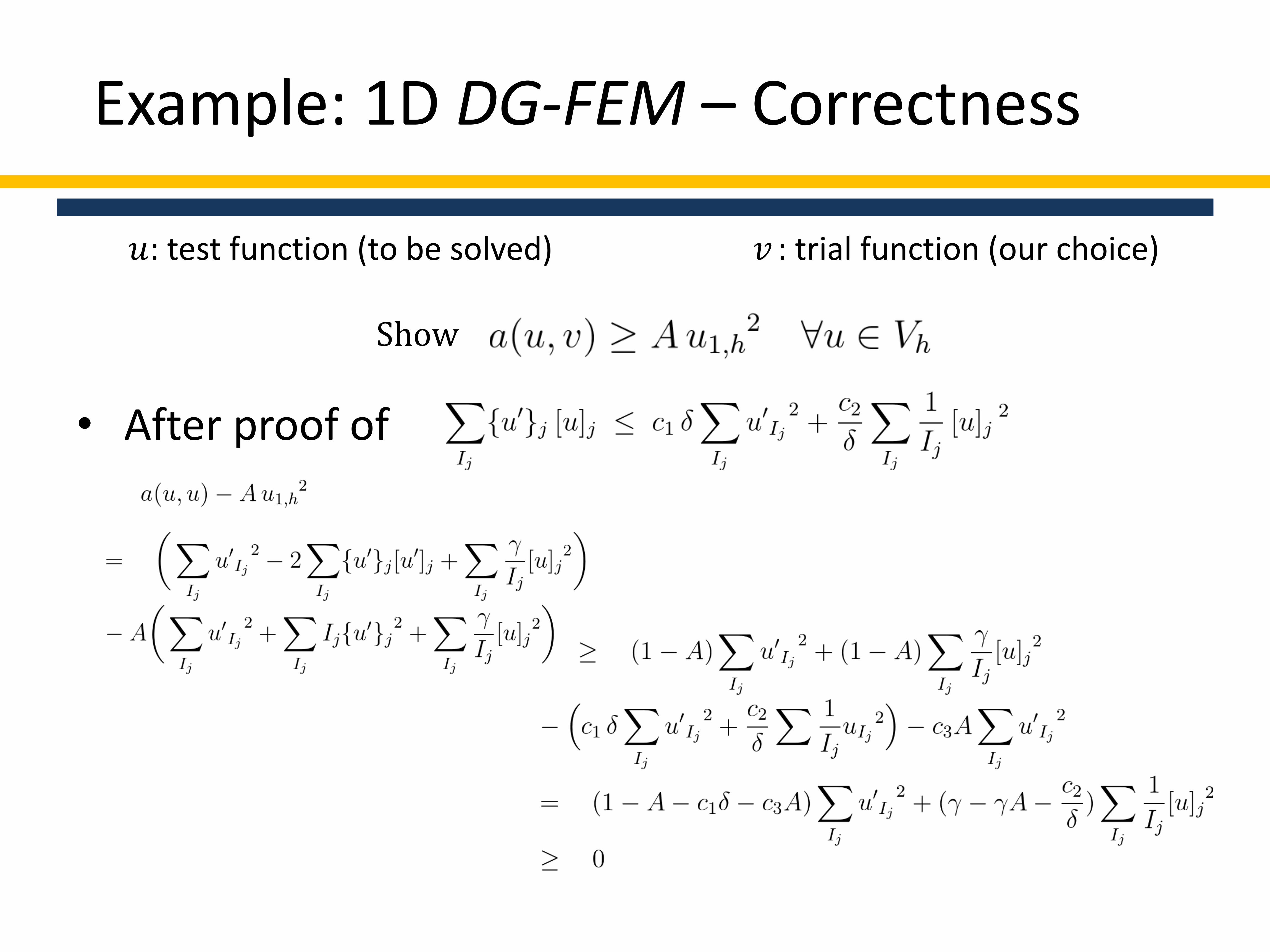
• After proof of



Show

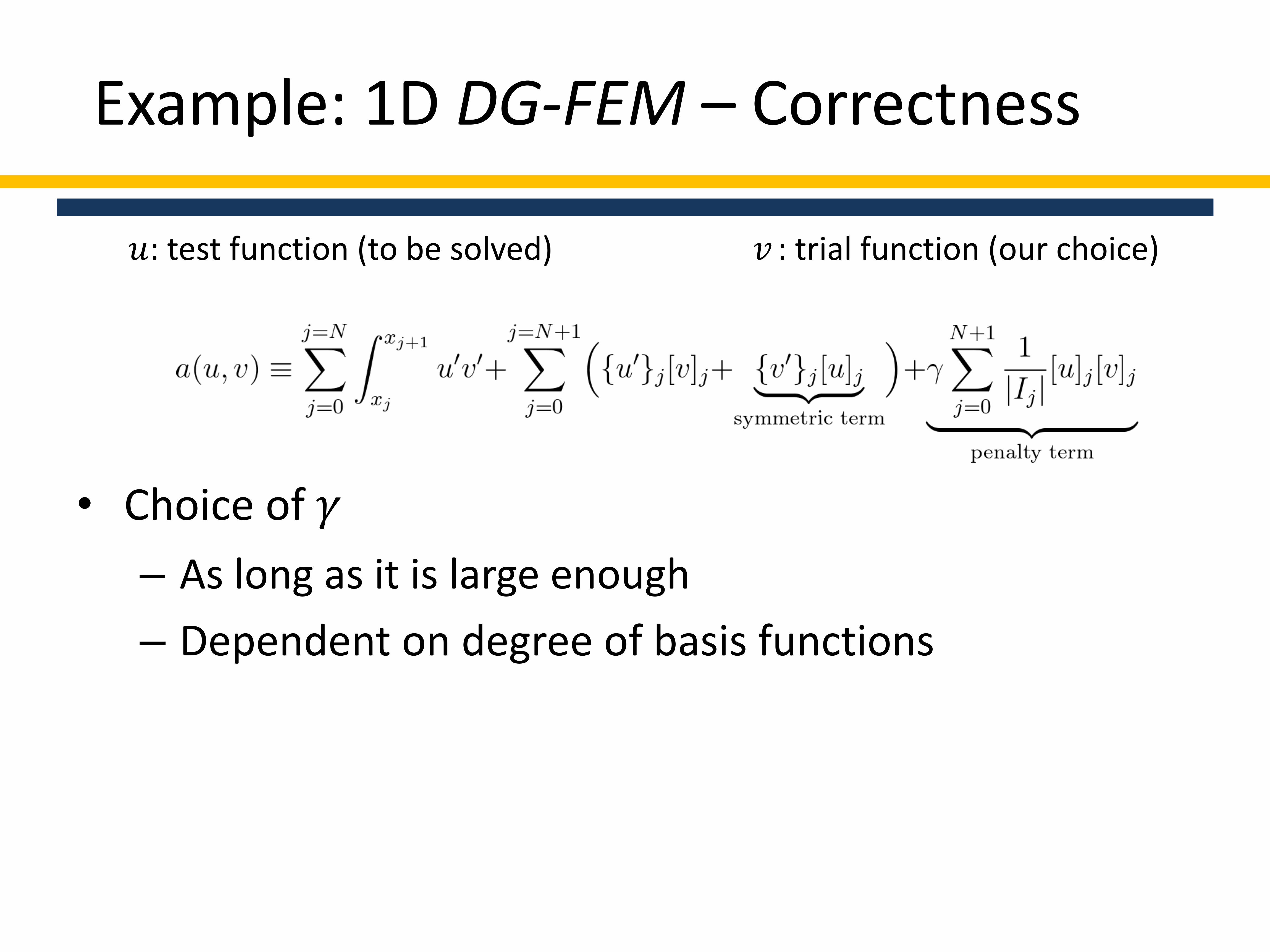
• Choice of 𝛾

– As long as it is large enough

– Dependent on degree of basis functions



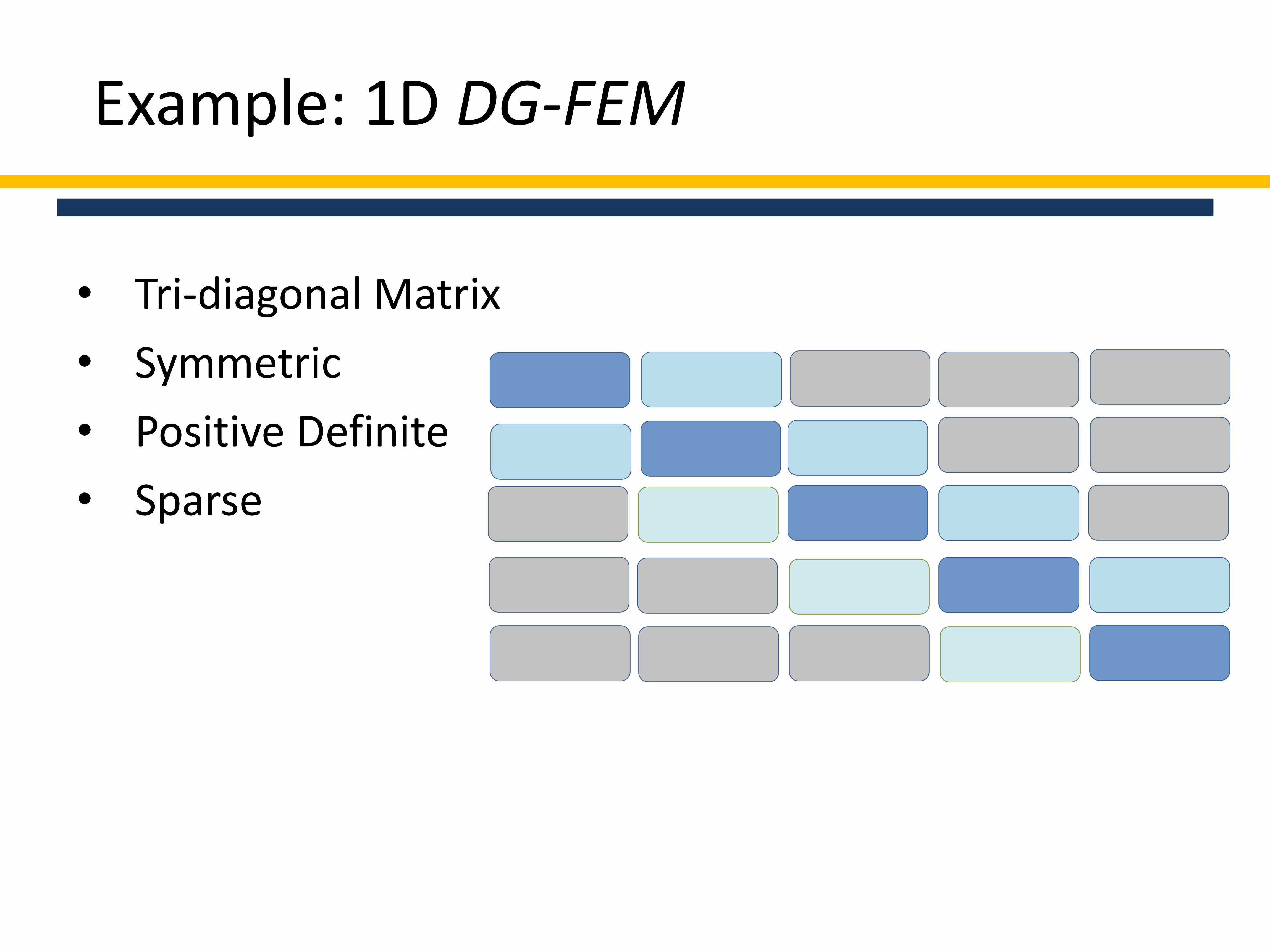
• Tri-diagonal Matrix

• Symmetric

• Positive Definite

• Sparse

Example: 1D DG-FEM

•Overview



•Future Work

•Acknowledgement

1D Parallelization: Why

• Higher accuracy …

…leads to larger matrix (and cost)

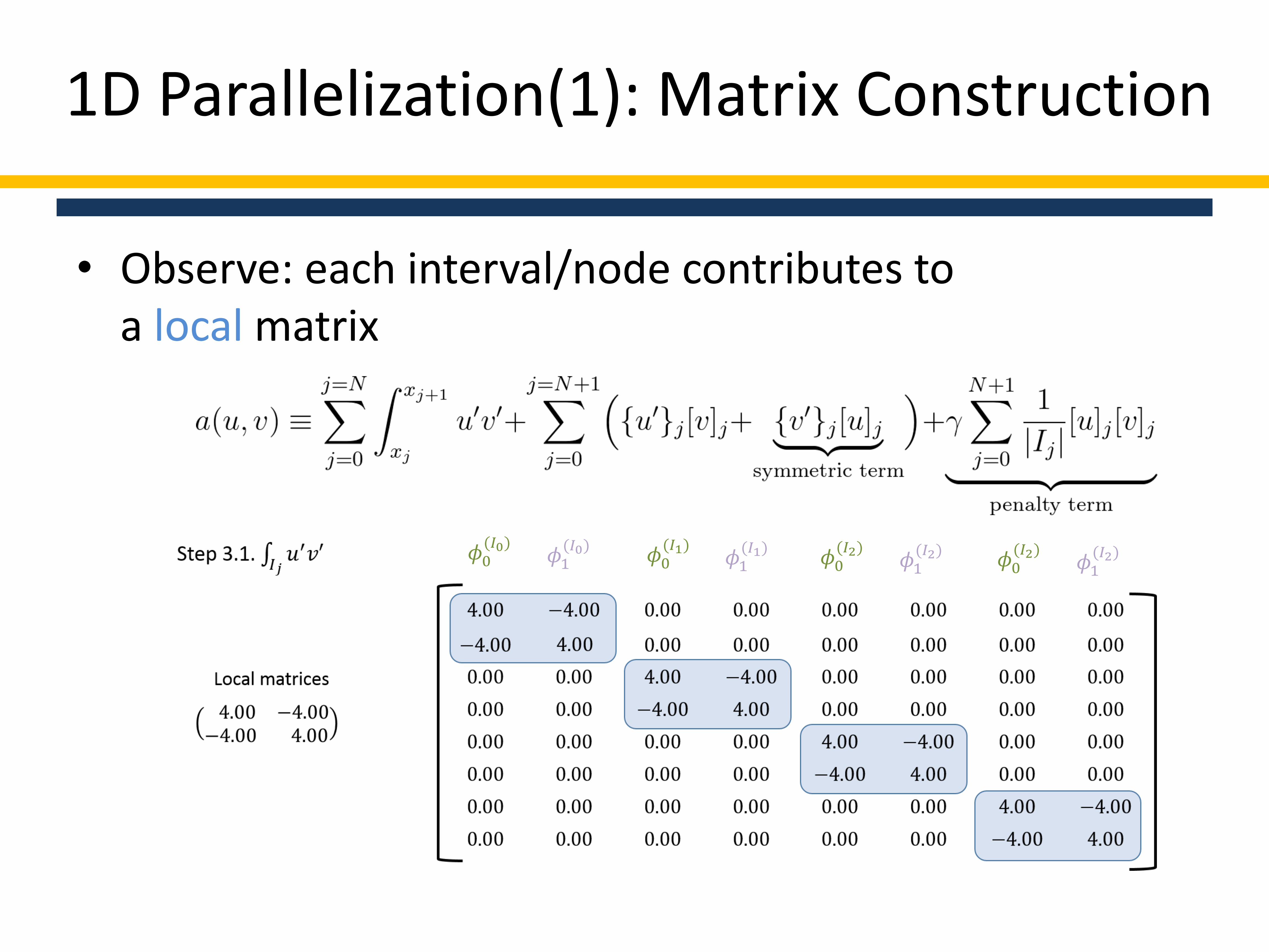
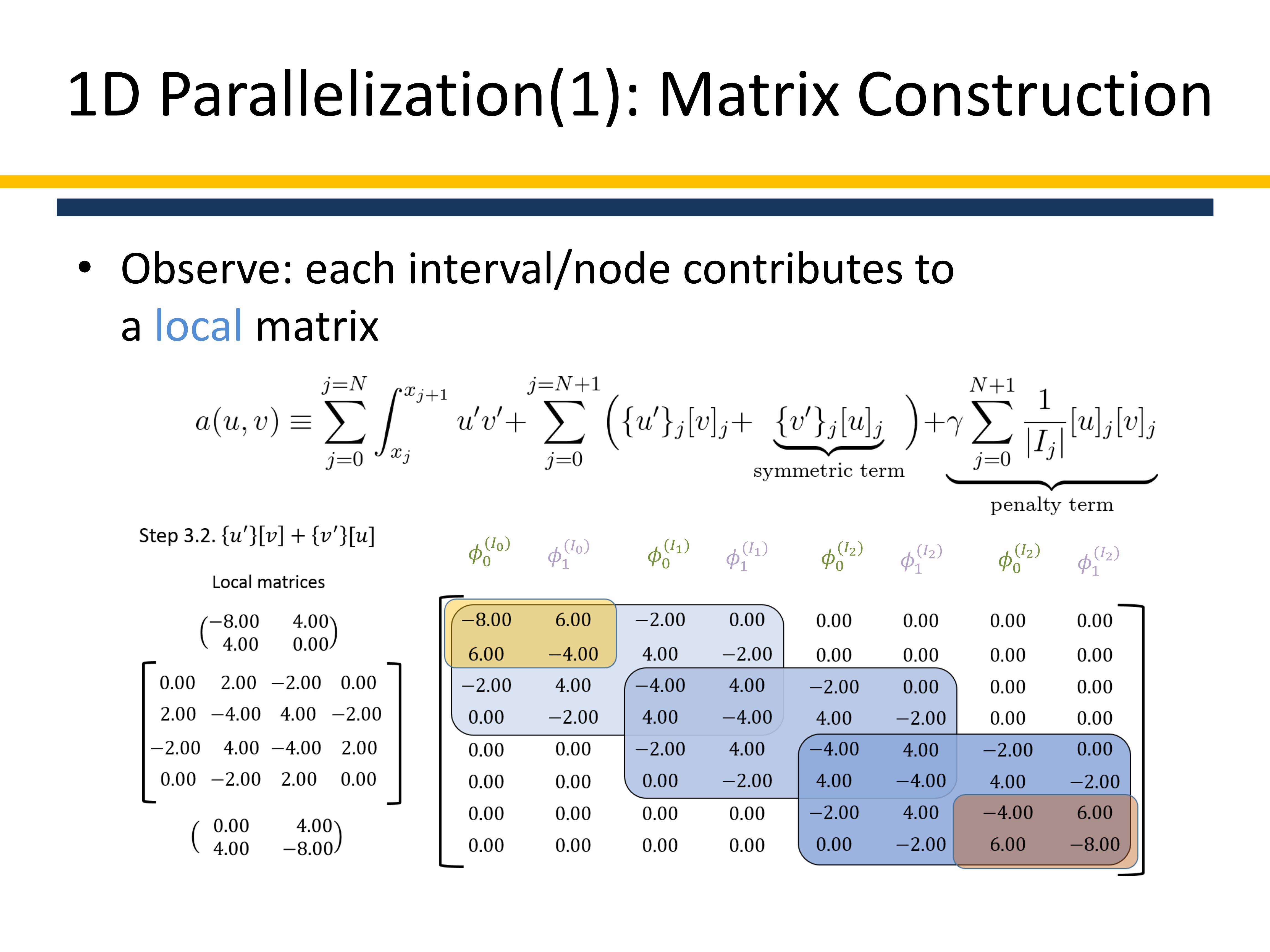
1D Parallelization(1): Matrix Construction

• Observe: each interval/node contributes toa local matrix

𝜙0(𝐼0)

𝜙1(𝐼0) 𝜙0

(𝐼1)𝜙1

(𝐼1) 𝜙0(𝐼2)

𝜙1(𝐼2) 𝜙0

(𝐼2)𝜙1

(𝐼2)


𝜙0(𝐼0)

𝜙1(𝐼0) 𝜙0

(𝐼1)𝜙1

(𝐼1) 𝜙0(𝐼2)

𝜙1(𝐼2) 𝜙0

(𝐼2)𝜙1

(𝐼2)



𝜙0(𝐼0)

𝜙1(𝐼0) 𝜙0

(𝐼1)𝜙1

(𝐼1) 𝜙0(𝐼2)

𝜙1(𝐼2) 𝜙0

(𝐼2)𝜙1

(𝐼2)


• Algorithm

• 1. Initialization: for each processor, receive information of P cells

2. Local Matrix Construction

for each processor for each of P cells, calculate the cell matrixcalculate the processor matrix

3. Global Matrix Construction

for root processorreceive information from other processorscalculate the global matrix (assembly)


Assemblydone by

MPI

Cell matrices

Processor matrices

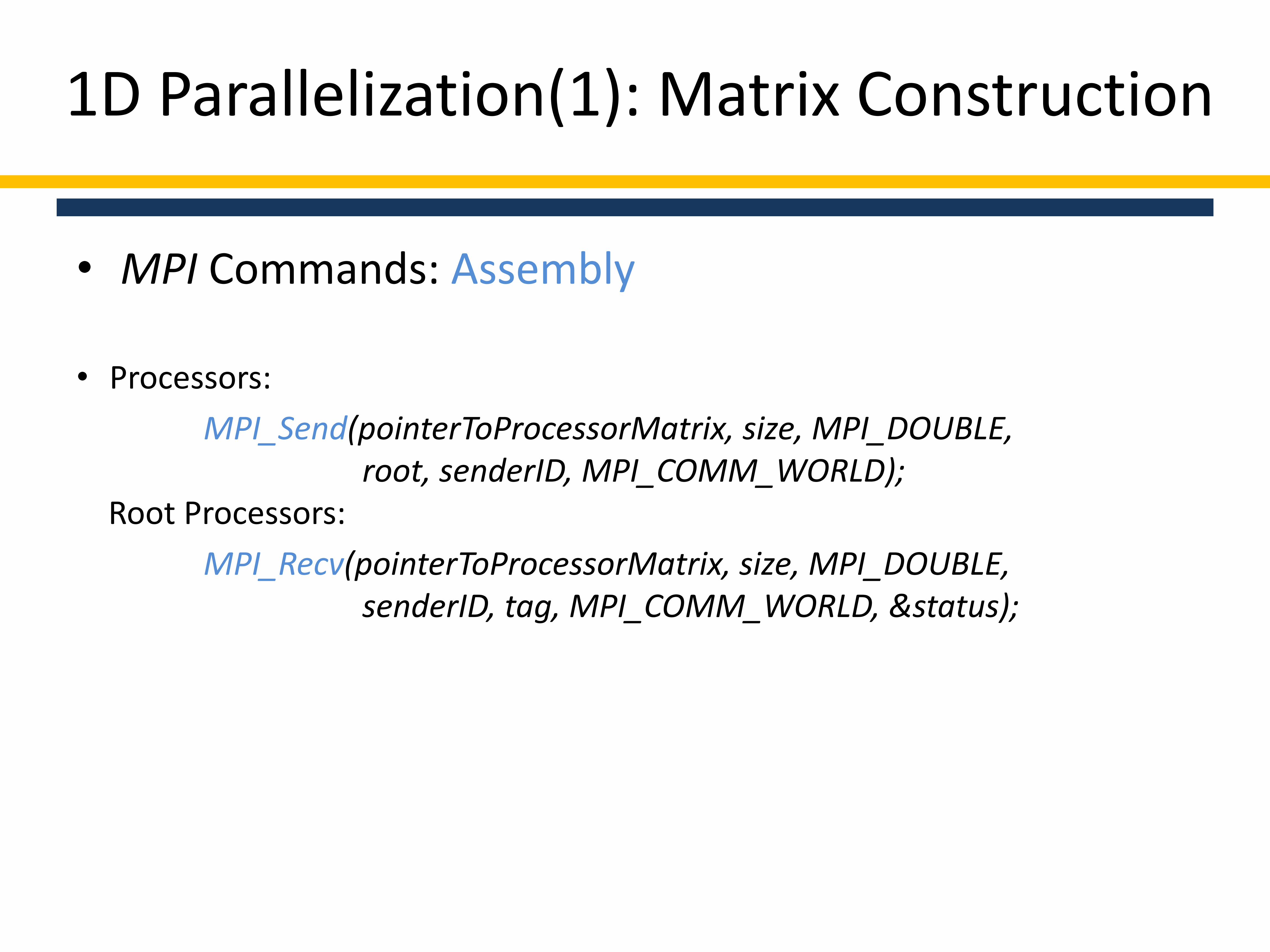
• MPI Commands: Assembly

• Processors:

MPI_Send(pointerToProcessorMatrix, size, MPI_DOUBLE,root, senderID, MPI_COMM_WORLD);

Root Processors:

MPI_Recv(pointerToProcessorMatrix, size, MPI_DOUBLE, senderID, tag, MPI_COMM_WORLD, &status);


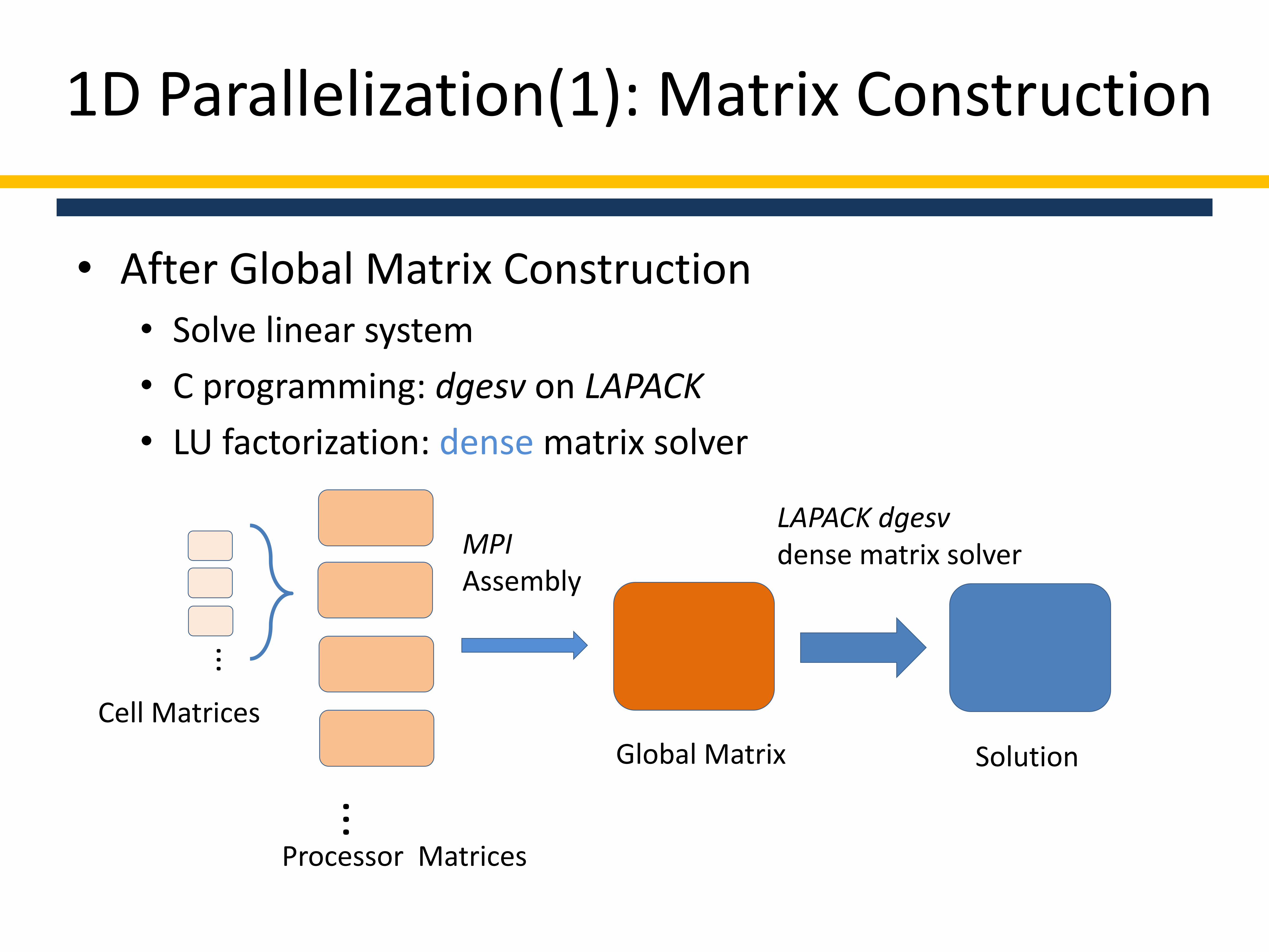
• After Global Matrix Construction• Solve linear system

• C programming: dgesv on LAPACK

• LU factorization: dense matrix solver


...

...

Cell Matrices

Processor Matrices

MPIAssembly

Global Matrix

LAPACK dgesvdense matrix solver

Solution

• Overall Matrix Construction Timedecreases with number of processors


Time (s)

No. of Processors

No. of Cells: 5,000,000Degree of freedom: 2

No. of Procs Time (s)

1 7.60062

2 4.13656s

4 2.22328s

8 1.34502s

16 0.67569s

32 0.36376s

64 0.17482s

“Can we do better?”

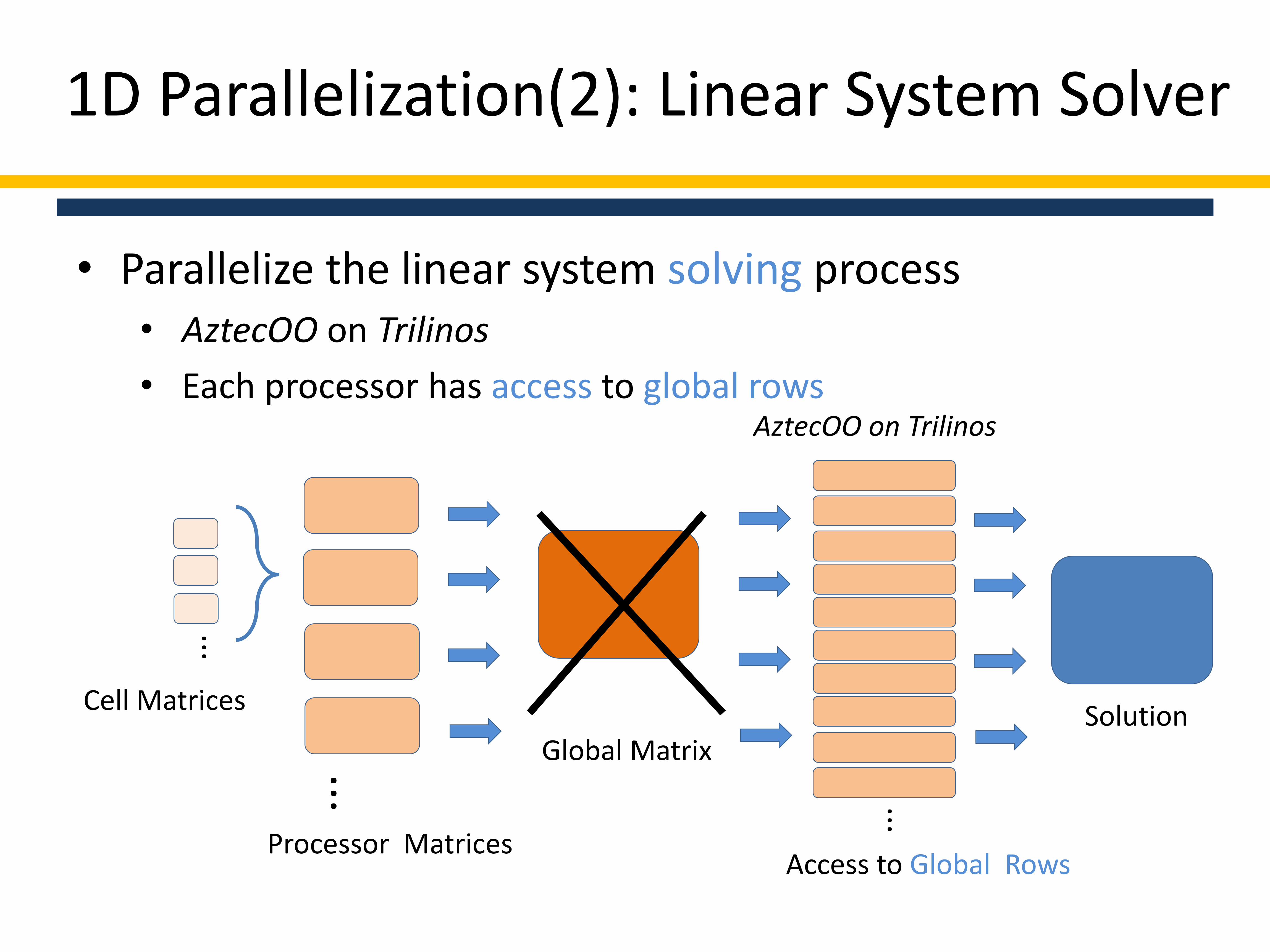
• Parallelize the linear system solving process• AztecOO on Trilinos

• Each processor has access to global rows

1D Parallelization(2): Linear System Solver

...

Cell Matrices

Processor Matrices

Global MatrixSolution

...

AztecOO on Trilinos

...

Access to Global Rows

• Trilinos Commands1. Define rows owned by each processor

Epetra_Map map(GlobalNumberOfRows, LocalNumberOfRows,GlobalIndicesOfRows, index, comm);

2. Send rows to global matrix position

InsertGlobalValues(GlobalIndexOfRows, NumOfEntries,

ValueOfEntries, GlobalColumnIndices);

3. Create solver

x = new Epetra_Vector(map);

problem = new Epetra_LinearProblem(GlobalMatrix, x, RHSvector);AztecOO solver(*problem);solver.Iterate(MaxNoOfIterations, Tolerance);


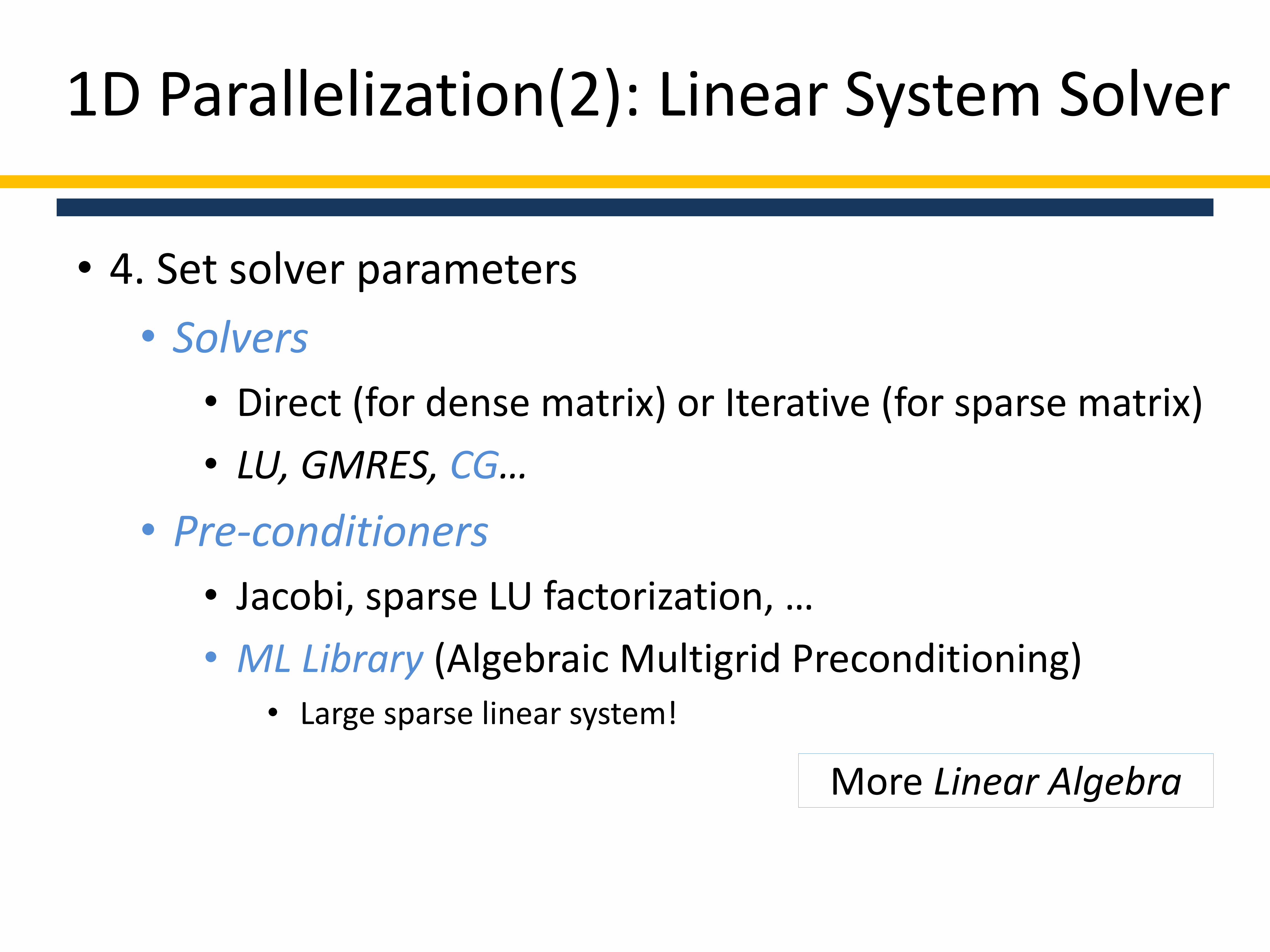
• 4. Set solver parameters

• Solvers

• Direct (for dense matrix) or Iterative (for sparse matrix)

• LU, GMRES, CG…

• Pre-conditioners

• Jacobi, sparse LU factorization, …

• ML Library (Algebraic Multigrid Preconditioning)• Large sparse linear system!


More Linear Algebra

• AztecOO Commands• solver.SetAztecOption(AZ_solver, SolverType);

• solver.SetAztecOption(AZ_precond, PreCondiType);

• ML preconditioner Commands• ML_Epetra::MultiLevelPreconditioner* MLPrec =

new ML_Epetra:: MultiLevelPreconditioner(GlobalMatrixPointer, Teuchos::ParameterList MLList, true);

• solver.SetPrecOperator(MLPrec)


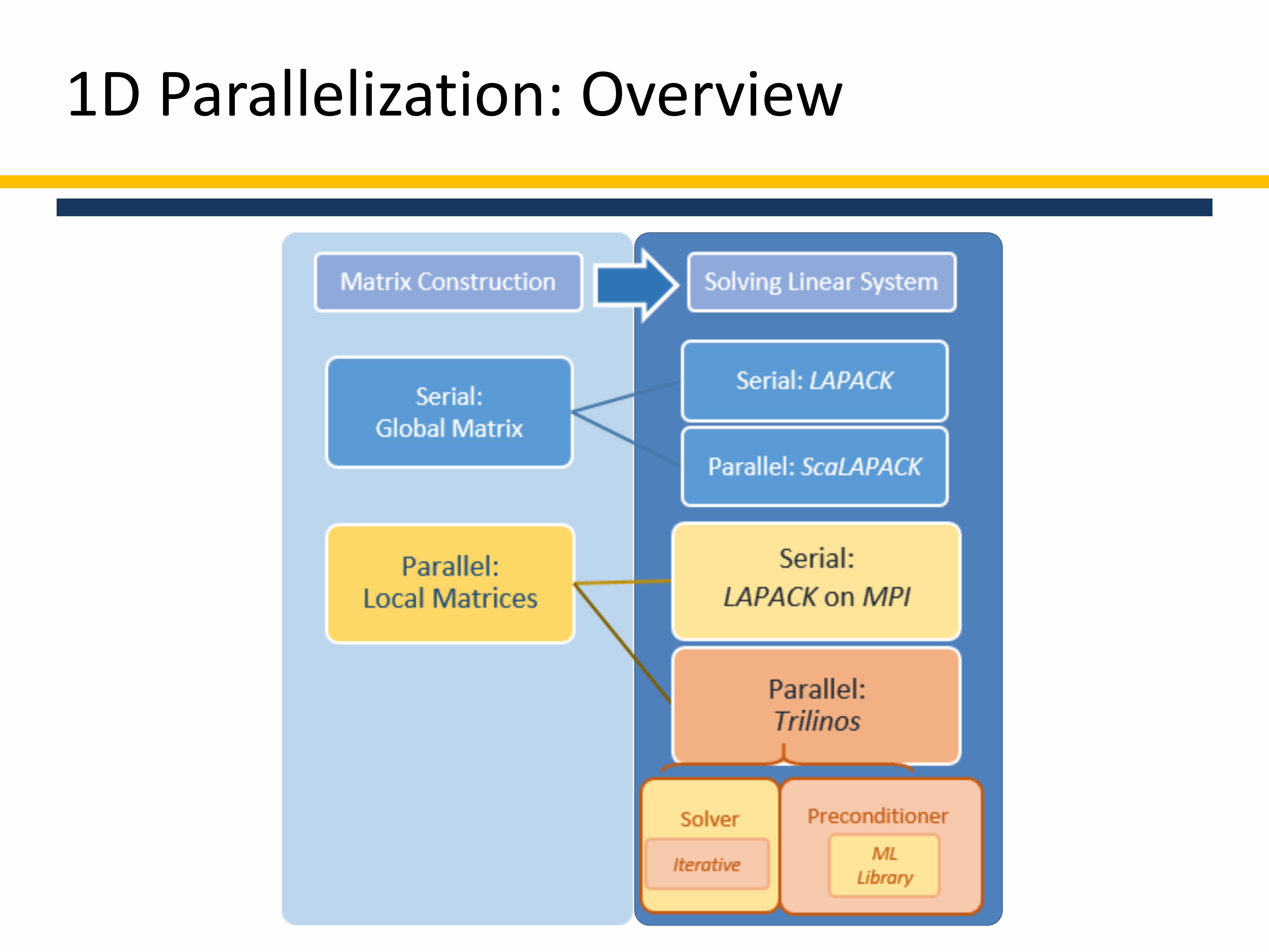
1D Parallelization: Overview

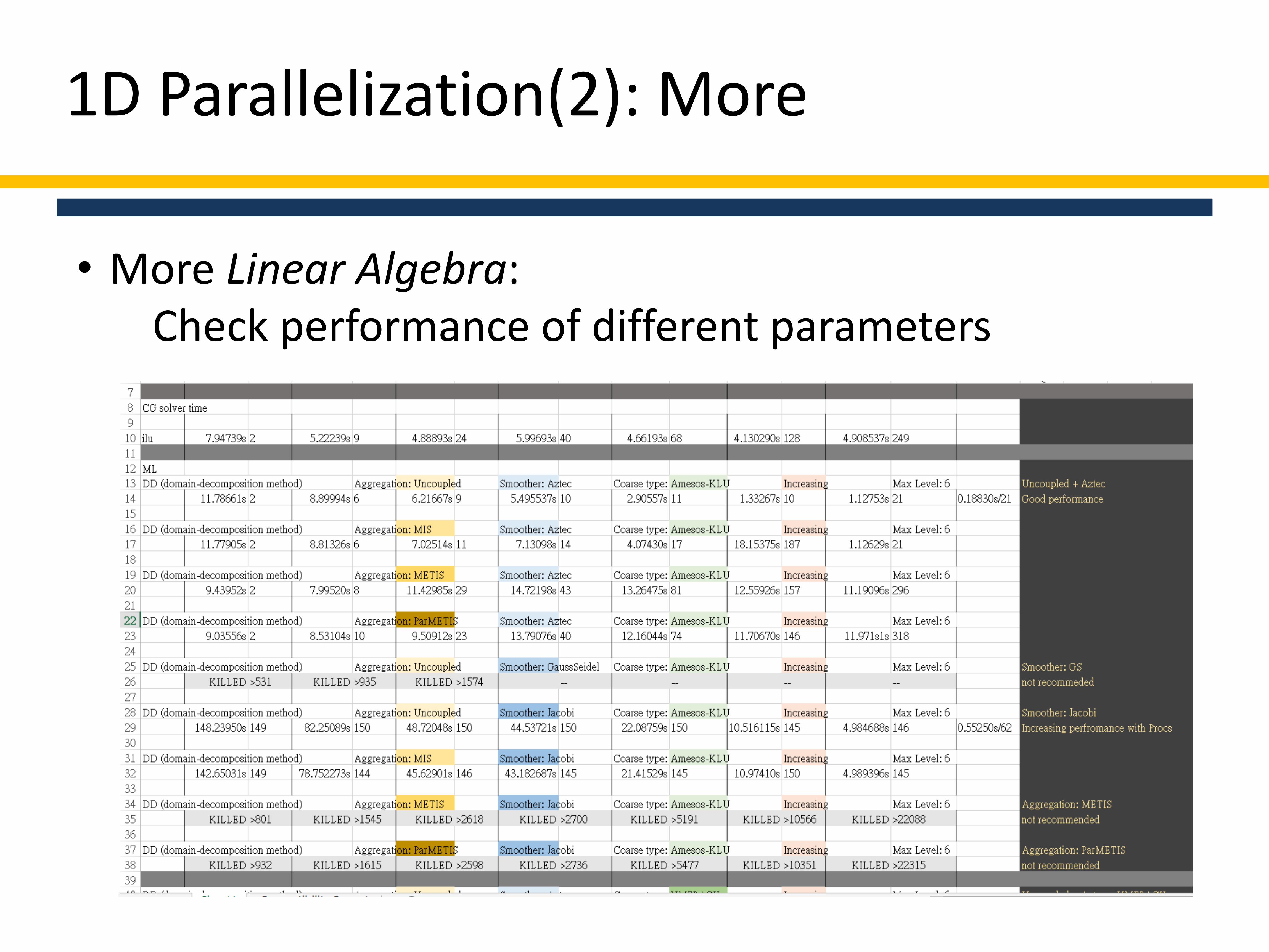
• More Linear Algebra:Check performance of different parameters

1D Parallelization(2): More

1D Parallelization(2): More

• Best performance found in ML• Domain-decomposition method

• Aggregation: Uncoupled

• Smoother: Aztec

• Coarse type: UMFPACK

Solver Time/ No. of Iterations

No. of Procs CG ML CG ilu

1 11.81769s/2 7.94730s/2

2 8.87170s/6 5.22223s/9

4 6.22301s/9 4.88893s/24

8 5.53356s/10 4.79693s/40

16 2.91182s/11 4.66193s/68

32 1.33327s/10 4.130290s/128

64 0.72338s/12 4.908537s/249

No. of Cells: 5,000,000Degree of freedom: 2

“Can we do better?”

•Overview



•Future Work

•Acknowledgement

Future Work: 2D DG-FEM

• Implement parallelization on 2D DG-FEM

• Partition of Domain: Triangles

• Jump condition over Edges


• Implement parallelization on 2D DG-FEM

• Weak form of FEM:

• Bilinear Function of DG-FEM:


• Correctness given by showing

where norm defined as

Future Work

• … and on 3D DG-FEM

• Adaptive Meshing• local refinement

• Application e.g. Chemical Transport Equation

•Overview



•Future Work

•Acknowledgement

Acknowledgement

This project was sponsored by

Oak Ridge National Laboratory, Joint Institute for Computational Sciences,

University of Tennessee, Knoxvilleand the Chinese University of Hong Kong.

Also sincere gratitude to my mentors Dr. Kwai Wong

and Dr. Ohannes Karakashian

Questions

Documents

Parallel Discontinuous Galerkin Method