FRIEDRICH-ALEXANDER-UNIVERSITAT ERLANGEN-NURNBERGINSTITUT FUR INFORMATIK (MATHEMATISCHE MASCHINEN UND DATENVERARBEITUNG)

Lehrstuhl fur Informatik 10 (Systemsimulation)

Multigrid HowTo: A simple Multigrid solver in C++ in less than 200 linesof code

Harald Kostler

Lehrstuhlbericht 08-3

Multigrid HowTo (Part I): A simple Multigrid solver in

C++ in less than 200 lines of code

Harald Kostler∗

Abstract

This short report is meant to guide multigrid beginners in order to implement theirfirst simple multigrid solver. We choose to show a 2D Poisson solver on a structuredcell-based grid that requires less than 200 lines of code. We will try to give a step-by-stepintroduction to multigrid from a practical point of view along this test implementation.

1 Introduction

In many areas of computation large linear or nonlinear systems have to be solved. Multigrid

is one method to solve such systems that have a certain structure, e.g. that arise from the

discretization of PDEs and lead to sparse and symmetric positive definite system matrices.

The advantages of multigrid solvers compared to other solvers are that multigrid methods are

applicable to a wide range of problems and can reach an asymptotically optimal complexity

of O(N), where N is the number of unknowns in the system.

The multigrid principle is first mentioned by Fedorenko [8, 9] and Bakhvalov [1] and

then intensively studied and pioneered by Brandt [2, 3] and Hackbusch [11]. For good

introductions and a comprehensive overview on multigrid methods, we, e.g., refer to [5, 19,

20, 21], for details on efficient multigrid implementations see [6, 7, 10, 12, 14, 15, 17, 18].

The MGNet Bibliography1 collects many articles related to multigrid. In the last years multi-

grid has been applied to many fields, e.g., fluid mechanics, meteorology, quantum chemistry,

bioelectric field computations, image processing, or computer vision.

Multigrid is not a single algorithm, but a general approach to find a solution by using

several levels or resolutions. We distinguish different types of multigrid techniques depending

on the meaning of a level. The structured or geometric multigrid (MG) identifies each level

with a (structured) grid.

Another approach applicable to general non-uniform or unstructured grids arising, e.g.,

from finite element discretizations on complex domains is algebraic multigrid (AMG) [4, 16].

∗harald.koestler@informatik.uni-erlangen.de1http://www.mgnet.org/bib/mgnet.bib

2

AMG works directly on the algebraic system of equations and one level is just a matrix of a

given size. Note that the adjacency graph of the matrix reveals the (unstructured) grid and

also geometric multigrid can be written as algebraic system of equations.

In this report we try to minimize the presentation of mathematical details and refer to

the literature instead [13]. Nevertheless, we have to formalize the given problem. We assume

that we want to solve the partial differential equation (PDE)

−∆u + αu = f in Ω (1a)

〈∇u,n〉 = 0 on ∂Ω (1b)

with (natural) Neumann boundary conditions on a rectangular domain Ω. Eq. (1) is dis-

cretized by finite differences on a structured grid what leads to a linear system

Ahuh = fh ,∑j∈Ωh

ahijuhj = fhi , i ∈ Ωh (2)

with system matrix Ah ∈ RN×N , unknown vector uh ∈ RN and right hand side (RHS)

vector fh ∈ RN on a discrete grid Ωh. n = 1h

denotes the number of unknowns in x- and

y-direction, and N = n2 the problem size. We assume that Ωh is a cell-based grid with mesh

size h = 12i , i ∈ N. In stencil notation the discretized eq. (1) reads

1

h2

0 −1 0

−1 4 −1

0 −1 0

uh +[α

]uh = fh, (3)

where the operator

Ah =

0 − 1h2 0

− 1h2

4h2 + α − 1

h2

0 − 1h2 0

. (4)

In order to solve the above linear system, we apply the multigrid idea that is based on

two principles:

Smoothing Property: Classical iterative methods like Gauß-Seidel (GS) are able to smooth

the error after very few steps. That means the high frequency components of the error are

removed well by these methods. But they have little effect on the low frequency components.

Therefore, the convergence rate of classical iterative methods is good in the first few steps

and decreases considerably afterwards.

Coarse Grid Principle: It is well known that a smooth function on a fine grid can be

approximated satisfactorily on a grid with less discretization points, whereas oscillating func-

tions would disappear. Furthermore, a procedure on a coarse grid is less expensive than on

a fine grid. The idea is now to approximate the low frequency error components on a coarse

grid.

3

The usual multigrid efficiency is achieved through the combination of two iterations, the

smoother, or relaxation, and the coarse grid correction. Here, the smoother reduces the

high frequency error components first, and then the low frequency error components are

approximated on coarser grids, interpolated back to the finer grids and eliminated there.

This leads to recursive algorithms which traverse between fine and coarse grids in the grid

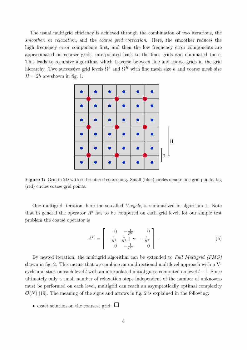
hierarchy. Two successive grid levels Ωh and ΩH with fine mesh size h and coarse mesh size

H = 2h are shown in fig. 1.

Figure 1: Grid in 2D with cell-centered coarsening. Small (blue) circles denote fine grid points, big(red) circles coarse grid points.

One multigrid iteration, here the so-called V-cycle, is summarized in algorithm 1. Note

that in general the operator Ah has to be computed on each grid level, for our simple test

problem the coarse operator is

AH =

0 − 1H2 0

− 1H2

4H2 + α − 1

H2

0 − 1H2 0

. (5)

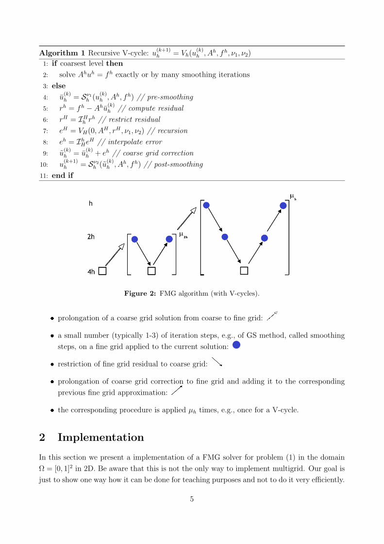
By nested iteration, the multigrid algorithm can be extended to Full Multigrid (FMG)

shown in fig. 2. This means that we combine an unidirectional multilevel approach with a V-

cycle and start on each level l with an interpolated initial guess computed on level l−1. Since

ultimately only a small number of relaxation steps independent of the number of unknowns

must be performed on each level, multigrid can reach an asymptotically optimal complexity

O(N) [19]. The meaning of the signs and arrows in fig. 2 is explained in the following:

exact solution on the coarsest grid:

4

Algorithm 1 Recursive V-cycle: u(k+1)h = Vh(u

(k)h , Ah, fh, ν1, ν2)

1: if coarsest level then

2: solve Ahuh = fh exactly or by many smoothing iterations

3: else

4: u(k)h = Sν1h (u

(k)h , Ah, fh) // pre-smoothing

5: rh = fh − Ahu(k)h // compute residual

6: rH = IHh rh // restrict residual

7: eH = VH(0, AH , rH , ν1, ν2) // recursion

8: eh = IhHeH // interpolate error

9: u(k)h = u

(k)h + eh // coarse grid correction

10: u(k+1)h = Sν2h (u

(k)h , Ah, fh) // post-smoothing

11: end if

Figure 2: FMG algorithm (with V-cycles).

prolongation of a coarse grid solution from coarse to fine grid:

a small number (typically 1-3) of iteration steps, e.g., of GS method, called smoothing

steps, on a fine grid applied to the current solution:

restriction of fine grid residual to coarse grid:

prolongation of coarse grid correction to fine grid and adding it to the corresponding

previous fine grid approximation:

the corresponding procedure is applied µh times, e.g., once for a V-cycle.

2 Implementation

In this section we present a implementation of a FMG solver for problem (1) in the domain

Ω = [0, 1]2 in 2D. Be aware that this is not the only way to implement multigrid. Our goal is

just to show one way how it can be done for teaching purposes and not to do it very efficiently.

5

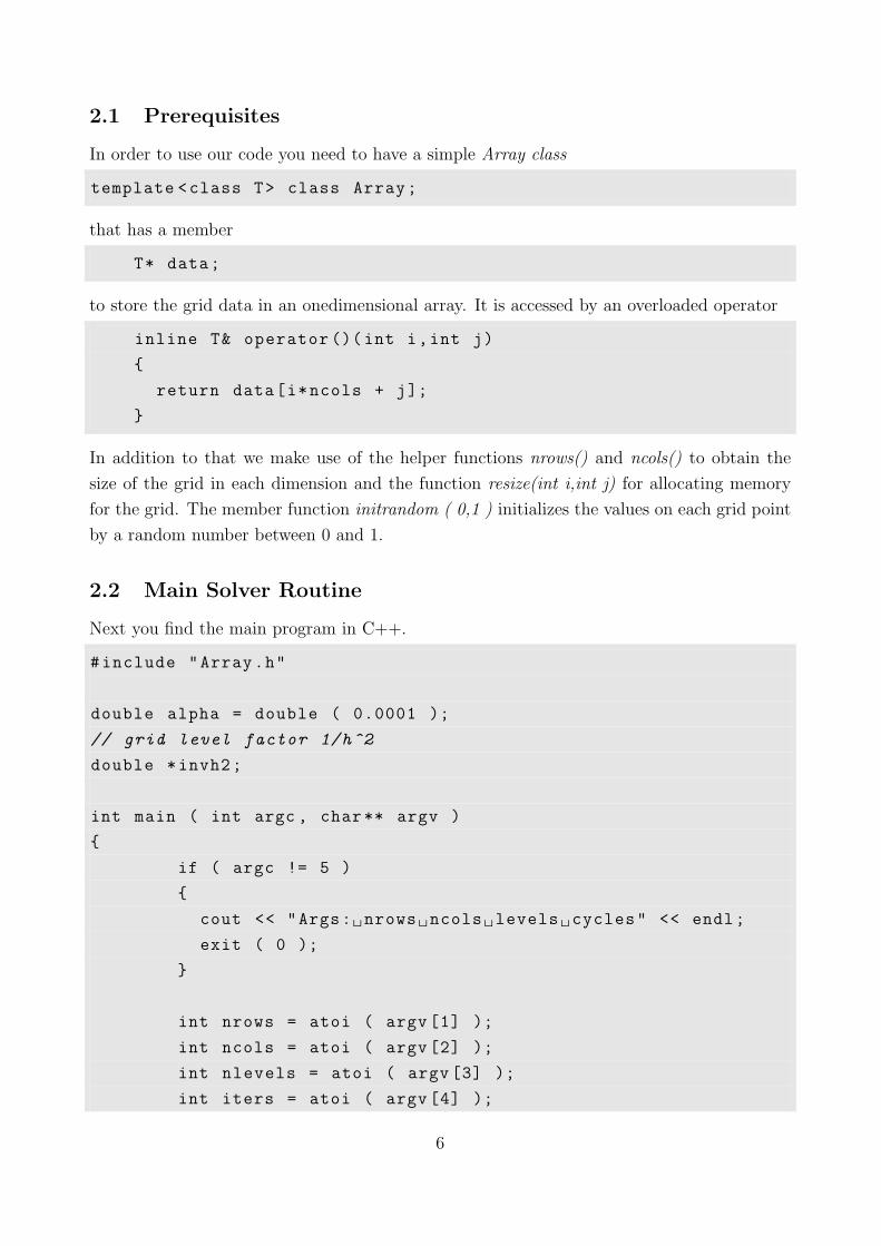
2.1 Prerequisites

In order to use our code you need to have a simple Array class

template <class T> class Array;

that has a member

T* data;

to store the grid data in an onedimensional array. It is accessed by an overloaded operator

inline T& operator ()(int i,int j)

return data[i*ncols + j];

In addition to that we make use of the helper functions nrows() and ncols() to obtain the

size of the grid in each dimension and the function resize(int i,int j) for allocating memory

for the grid. The member function initrandom ( 0,1 ) initializes the values on each grid point

by a random number between 0 and 1.

2.2 Main Solver Routine

Next you find the main program in C++.

#include "Array.h"

double alpha = double ( 0.0001 );

// grid level factor 1/h^2

double *invh2;

int main ( int argc , char** argv )

if ( argc != 5 )

cout << "Args: nrows ncols levels cycles" << endl;

exit ( 0 );

int nrows = atoi ( argv [1] );

int ncols = atoi ( argv [2] );

int nlevels = atoi ( argv [3] );

int iters = atoi ( argv [4] );

6

// Solution and right hand side on each level

Array <double >* Sol = new Array <double >[ nlevels ];

Array <double >* RHS = new Array <double >[ nlevels ];

// add 1 ghost layer in each direction

int sizeadd = 2;

invh2 = new double[nlevels ];

// allocate memory on each grid level

for ( int i = 0; i < nlevels; i++ )

Sol[i]. resize ( nrows+sizeadd ,ncols+sizeadd );

RHS[i]. resize ( nrows+sizeadd ,ncols+sizeadd );

nrows= ( nrows /2 );

ncols= ( ncols /2 );

invh2[i] = double ( 1.0 )

/ ( pow ( double ( 4.0 ),i ) );

// initialize solution and right hand side

Sol[nlevels -1]. initrandom ( 0,1 );

Sol [0] = 1;

// simply set f = 0 to obtain the solution u = 0

RHS [0] = 0;

// restrict right hand side to all coarse grids

for ( int i = 1; i < nlevels; i++ )

Restrict ( RHS[i-1],RHS[i] );

// compute normalized starting residual

double res_0 = residual ( 0,Sol ,RHS );

cout << "Starting residual: " << res_0 << endl;

// call FMG solver

cout << "Residual after FMG iteration: " <<

FMG_Solver(Sol , RHS , nlevels , iters , res_0)

<< endl;

7

delete [] invh2;

delete [] Sol;

delete [] RHS;

return 0;

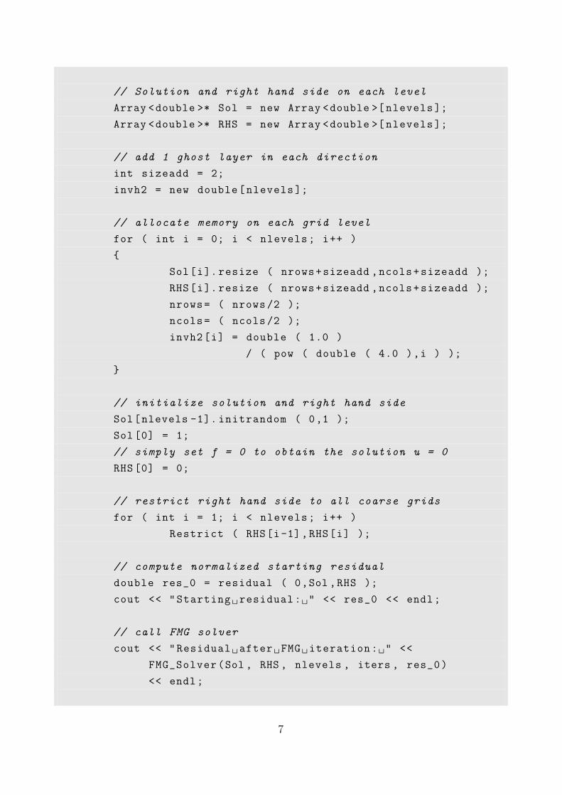
After reading the command line arguments, the number of grid points in x- and y- direc-

tion, the number of multigrid levels and the number of multigrid V-cycles to perform, the

memory for solution and right hand side on each grid level is allocated and both are initialized.

Note that the coarser levels become smaller by a factor of 2 in each direction per additional

grid level. For the treatment of Neumann boundary conditions, we add one additional layer

of so-called ghost cells around each grid. The lines

invh2[i] = double ( 1.0 )

/ ( pow ( double ( 4.0 ),i ) );

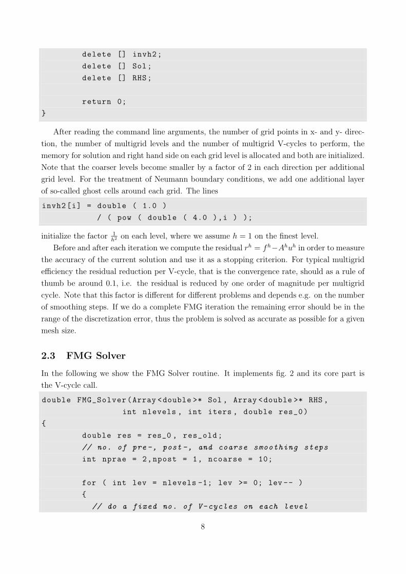
initialize the factor 1h2 on each level, where we assume h = 1 on the finest level.

Before and after each iteration we compute the residual rh = fh−Ahuh in order to measure

the accuracy of the current solution and use it as a stopping criterion. For typical multigrid

efficiency the residual reduction per V-cycle, that is the convergence rate, should as a rule of

thumb be around 0.1, i.e. the residual is reduced by one order of magnitude per multigrid

cycle. Note that this factor is different for different problems and depends e.g. on the number

of smoothing steps. If we do a complete FMG iteration the remaining error should be in the

range of the discretization error, thus the problem is solved as accurate as possible for a given

mesh size.

2.3 FMG Solver

In the following we show the FMG Solver routine. It implements fig. 2 and its core part is

the V-cycle call.

double FMG_Solver(Array <double >* Sol , Array <double >* RHS ,

int nlevels , int iters , double res_0)

double res = res_0 , res_old;

// no. of pre-, post -, and coarse smoothing steps

int nprae = 2,npost = 1, ncoarse = 10;

for ( int lev = nlevels -1; lev >= 0; lev -- )

// do a fixed no. of V-cycles on each level

8

for ( int i = 0; i < iters; i++ )

res_old = res;

VCycle ( lev ,Sol ,RHS ,nprae ,npost ,ncoarse ,nlevels );

// compute residual as accuracy measure

res = residual ( lev ,Sol , RHS );

cout << "FMG level: " << lev << " cycle: "

<< i << " residual: " << res

<< " residual reduction: " << res_0/res

<< " convergence factor: "

<< res/res_old << endl;

// if not finest level interpolate current solution

if ( lev > 0 )

interpolate ( Sol[lev -1],Sol[lev],lev );

return res;

The V-cycle itself is the most time consuming part in the multigrid solver and within the

V-cycle, the smoother takes usually most of the time.

void VCycle ( int lev ,Array <double >* Sol , Array <double >* RHS ,

int nprae , int npost , int ncoarse , int nlevels )

// solve problem on coarsest grid ...

if ( lev == nlevels -1 )

for ( int i = 0; i < ncoarse; i++ )

GaussSeidel ( lev , Sol , RHS );

else

// ... or recursively do V-cycle

// do some presmoothing steps

for ( int i = 0; i < nprae; i++ )

GaussSeidel ( lev , Sol , RHS );

9

// compute and restrict the residual

Restrict_Residual ( lev , Sol , RHS );

// initialize the coarse solution to zero

Sol[lev+1] = 0;

VCycle ( lev+1,Sol ,RHS ,nprae ,npost ,ncoarse ,nlevels );

// interpolate error and correct fine solution

interpolate_correct ( Sol[lev], Sol[lev+1], lev+1 );

// do some postsmoothing steps

for ( int i = 0; i < npost; i++ )

GaussSeidel ( lev , Sol , RHS );

Note that on the coarsest grid also a direct solver can be used.

2.4 Gauss-Seidel Smoother

Since most of the time is spent in the smoother, it should be implemented efficiently. Never-

theless, we present a straightforward implementation for simplicity. The core routine solves

eq. (3) by looping over all grid points in the domain and fixing all unknowns except the cur-

rent grid point. Therefore the problem reduces to the solution of an equation with only one

unknown what can be done very easily.

void GaussSeidel (int lev ,Array <double >* Sol ,Array <double >* RHS)

double denom = double ( 1.0 )

/ ( double (4.0) * invh2[lev] + alpha );

// assure boundary conditions

treatboundary ( lev ,Sol );

// Gauss -Seidel relaxation with damping parameter

for ( int i=1; i<Sol[lev]. nrows ()-1; i++ )

for ( int j=1; j<Sol[lev]. ncols ()-1; j++ )

10

Sol[lev] ( i,j ) = ( RHS[lev] ( i,j ) +

invh2[lev]* (Sol[lev](i+1,j) + Sol[lev](i-1,j) +

Sol[lev](i,j+1) + Sol[lev](i,j-1) )

) * denom;

// assure boundary conditions

treatboundary ( lev ,Sol );

In order to treat the Neumann boundary conditions we explicitly copy the solution from

the boundary into the ghost layers.

void treatboundary ( int lev ,Array <double >* Sol )

// treat left and right boundary

for ( int i=0; i<Sol[lev]. nrows (); i++ )

Sol[lev] ( i,0 ) = Sol[lev] ( i,1 );

Sol[lev] ( i,Sol[lev]. ncols()-1 ) =

Sol[lev] ( i,Sol[lev]. ncols()-2 );

// treat upper and lower boundary

for ( int j=0; j<Sol[lev]. ncols (); j++ )

Sol[lev] ( 0,j ) = Sol[lev] ( 1,j );

Sol[lev] ( Sol[lev].nrows()-1,j ) =

Sol[lev] ( Sol[lev]. nrows()-2,j );

2.5 Residual and Restriction Routines

The residual is computed in the L2 norm by

double residual ( int lev ,Array <double >* Sol ,Array <double >* RHS )

11

double res = double ( 0.0 );

double rf;

for ( int i=1; i<Sol[lev]. nrows ()-1; i++ )

for ( int j=1; j<Sol[lev]. ncols ()-1; j++ )

rf = RES ( i,j );

res += rf*rf;

return sqrt ( res )

/ ( Sol[lev].nrows () * Sol[lev]. ncols() );

with

#define RES(i,j) (RHS[lev](i,j) + invh2[lev]*( Sol[lev](i+1,j)

+ Sol[lev](i,j+1) + Sol[lev](i,j-1)

+ Sol[lev](i-1,j) )

- (4.0* invh2[lev] + alpha)*Sol[lev](i,j))

what corresponds to fh−Ahuh at a given grid point (i, j). Next the grid transfers are printed.

Within the FMG algorithm we need a simple restriction routine one a fine grid into a coarse

one. The value of a coarse grid point is computed by a weighted sum of the surrounding fine

grid points, this can be written in stencil notation by

IHh =1

4

1 1

·1 1

. (6)

void Restrict ( Array <double >& fine ,Array <double >& coarse )

// loop over coarse grid points

for ( int i=1; i<coarse.nrows ()-1; i++ )

int fi = 2*i;

for ( int j=1; j<coarse.ncols ()-1; j++ )

int fj = 2*j;

coarse ( i,j ) = double ( 0.25 ) *

( fine ( fi , fj ) + fine ( fi -1, fj ) +

12

fine ( fi, fj -1 ) + fine ( fi -1, fj -1 ) );

During the V-cycle we have to compute the residual and to restrict it to the next coarser

grid level. This is done together in one routine.

void Restrict_Residual ( int lev ,Array <double >* Sol ,

Array <double >* RHS )

// loop over coarse grid points

for ( int i=1; i<RHS[lev +1]. nrows ()-1; i++ )

int fi = 2*i;

for ( int j=1; j<RHS[lev +1]. ncols ()-1; j++ )

int fj = 2*j;

RHS[lev+1] ( i,j ) = double ( 0.25 ) *

(RES( fi , fj ) + RES( fi -1, fj ) +

RES( fi, fj -1 ) + RES( fi -1, fj -1 ));

2.6 Interpolation Routines

For the transfer from a coarse to a fine grid we use a simple constant cell-based interpolation,

where the value of each coarse grid point is just distributed to its fine neighbors, written in

stencil notation

IhH =

1 1

·1 1

. (7)

void interpolate ( Array <double >& uf,Array <double >& uc,int l )

double v;

// loop over coarse grid points

for ( int i=1;i <uc.nrows ()-1;i++ )

13

int fi = 2*i;

for ( int j=1;j < uc.ncols ()-1;j++ )

int fj = 2*j;

v = uc ( i,j );

uf ( fi,fj ) = v;

uf ( fi -1,fj ) = v;

uf ( fi,fj -1 ) = v;

uf ( fi -1,fj -1 ) = v;

The interpolation of the approximated error from the coarse grid and the correction of the

current solution is again done in a single routine.

void interpolate_correct ( Array <double >& uf,

Array <double >& uc,int l )

double v;

// loop over coarse grid points

for ( int i=1;i <uc.nrows ()-1;i++ )

int fi = 2*i;

for ( int j=1;j < uc.ncols ()-1;j++ )

int fj = 2*j;

v = uc ( i,j );

uf ( fi,fj ) += v;

uf ( fi -1,fj ) += v;

uf ( fi,fj -1 ) += v;

uf ( fi -1,fj -1 ) += v;

14

3 Costs and Test Run

In this section we want to provide some insight on the performance of the code. First we

summarize the costs for the multigrid solver parts in table 1.

Table 1: Costs per unknown on one grid level: read and write accesses, number of integer operationsand number of floating point operations.

part read write Ops FOps

smoother 5 1 4 6

restrict residual 0.25 6 5.5 10

interpolate correct 0.25 1 1.5 1

residual 6 1 4 11

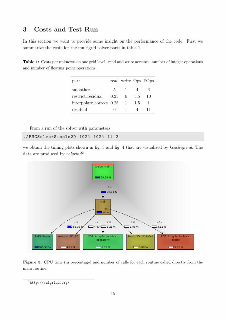
From a run of the solver with parameters

./ FMGSolverSimple2D 1024 1024 11 2

we obtain the timing plots shown in fig. 3 and fig. 4 that are visualized by kcachegrind. The

data are produced by valgrind2.

Figure 3: CPU time (in percentage) and number of calls for each routine called directly from themain routine.

2http://valgrind.org/

15

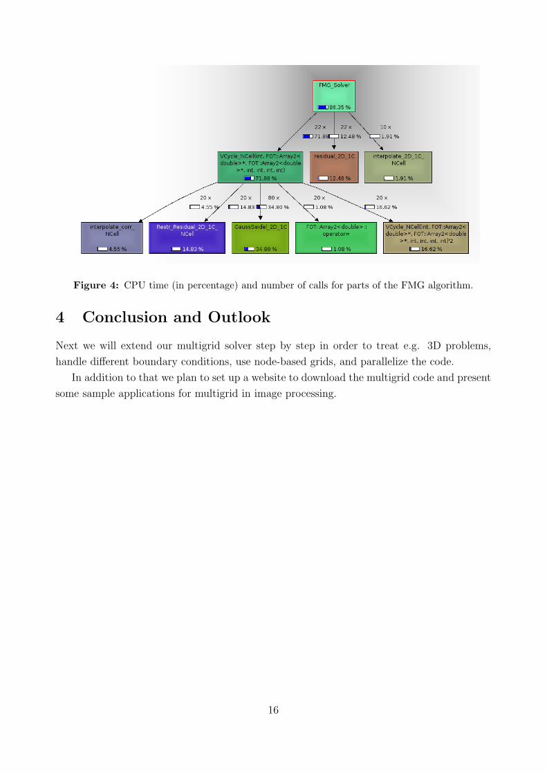
Figure 4: CPU time (in percentage) and number of calls for parts of the FMG algorithm.

4 Conclusion and Outlook

Next we will extend our multigrid solver step by step in order to treat e.g. 3D problems,

handle different boundary conditions, use node-based grids, and parallelize the code.

In addition to that we plan to set up a website to download the multigrid code and present

some sample applications for multigrid in image processing.

16

References

[1] N. Bakhvalov, “On the convergence of a relaxation method under natural constraints on

an elliptic operator,” Z. Vycisl. Mat. i. Mat. Fiz., vol. 6, pp. 861–883, 1966.

[2] A. Brandt, “Multi-Level Adaptive Solutions to Boundary-Value Problems,” Mathematics

of Computation, vol. 31, no. 138, pp. 333–390, 1977.

[3] ——, “Multigrid techniques: 1984 guide with applications to fluid dynamics,” GMD-

Studie Nr. 85, Sankt Augustin, West Germany, 1984.

[4] ——, “Algebraic multigrid theory: The symmetric case,” Applied Mathematics and Com-

putation, vol. 19, no. 1-4, pp. 23–56, 1986.

[5] W. Briggs, V. Henson, and S. McCormick, A Multigrid Tutorial, 2nd ed. Society for

Industrial and Applied Mathematics (SIAM), Philadelphia, PA, USA, 2000.

[6] I. Christadler, H. Kostler, and U. Rude, “Robust and efficient multigrid techniques

for the optical flow problem using different regularizers,” in Proceedings of 18th Sym-

posium Simulationstechnique ASIM 2005, ser. Frontiers in Simulation, F. Hulsemann,

M. Kowarschik, and U. Rude, Eds., vol. 15. SCS Publishing House, Erlangen, Germany,

2005, pp. 341–346, preprint version published as Tech. Rep. 05-6.

[7] C. Douglas, J. Hu, M. Kowarschik, U. Rude, and C. Weiß, “Cache Optimization for

Structured and Unstructured Grid Multigrid,” Electronic Transactions on Numerical

Analysis (ETNA), vol. 10, pp. 21–40, 2000.

[8] R. Fedorenko, “A relaxation method for solving elliptic difference equations,” USSR

Comput. Math. Phys, vol. 1, pp. 1092–1096, 1961.

[9] ——, “The speed of convergence of one iterative process,” USSR Comp. Math. and Math.

Physics, vol. 4, pp. 227–235, 1964.

[10] T. Gradl, C. Freundl, H. Kostler, and U. Rude, “Scalable Multigrid,” in High Per-

formance Computing in Science and Engineering. Garching/Munich 2007, S. Wagner,

M. Steinmetz, A. Bode, and M. Brehm, Eds., LRZ, KONWIHR. Springer-Verlag,

Berlin, Heidelberg, New York, 2008, pp. 475–483.

[11] W. Hackbusch, Multi-Grid Methods and Applications. Springer-Verlag, Berlin, Heidel-

berg, New York, 1985.

[12] F. Hulsemann, M. Kowarschik, M. Mohr, and U. Rude, “Parallel geometric multigrid,”

in Numerical Solution of Partial Differential Equations on Parallel Computers, ser. Lec-

ture Notes in Computational Science and Engineering, A. Bruaset and A. Tveito, Eds.

Springer-Verlag, Berlin, Heidelberg, New York, 2005, vol. 51, ch. 5, pp. 165–208.

17

[13] H. Kostler, “A Multigrid Framework for Variational Approaches in Medical Image

Processing and Computer Vision,” Ph.D. dissertation, Friedrich-Alexander-Universitat

Erlangen-Nurnberg, 2008.

[14] H. Kostler, M. Sturmer, and U. Rude, “A fast full multigrid solver for applications in

image processing,” Numerical Linear Algebra with Applications, vol. 15, no. 2–3, pp.

187–200, 2008.

[15] M. Kowarschik, C. Weiß, and U. Rude, “DiMEPACK — A Cache–Optimized Multigrid

Library,” in Proceedings of the Int. Conference on Parallel and Distributed Processing

Techniques and Applications (PDPTA 2001), H. Arabnia, Ed., vol. I. Las Vegas, NV,

USA: CSREA Press, Irvine, CA, USA, 2001, pp. 425–430.

[16] J. Ruge and K. Stuben, “Algebraic multigrid (AMG),” in Multigrid Methods, ser. Fron-

tiers in Applied Mathematics, S. McCormick, Ed. Society for Industrial and Applied

Mathematics (SIAM), Philadelphia, PA, USA, 1987, vol. 5, pp. 73–130.

[17] M. Sturmer, J. Treibig, and U. Rude, “Optimizing a 3D multigrid algorithm for the IA-

64 architecture,” in Proceedings of 18th Symposium Simulationstechnique ASIM 2006,

Hannover, ser. Frontiers in Simulation, M. Becker and H. Szczerbicka, Eds., vol. 16.

SCS Publishing House, Erlangen, Germany, 2006, pp. 271–276.

[18] M. Sturmer, G. Wellein, G. Hager, H. Kostler, and U. Rude, “Challenges and Potentials

of Emerging Multicore Architectures,” in High Performance Computing in Science and

Engineering. Garching/Munich 2007, S. Wagner, M. Steinmetz, A. Bode, and M. Brehm,

Eds., LRZ, KONWIHR. Springer-Verlag, Berlin, Heidelberg, New York, 2008, pp. 551–

566.

[19] U. Trottenberg, C. Oosterlee, and A. Schuller, Multigrid. Academic Press, San Diego,

CA, USA, 2001.

[20] P. Wesseling, Multigrid Methods. Edwards, Philadelphia, PA, USA, 2004.

[21] R. Wienands and W. Joppich, Practical Fourier Analysis for Multigrid Methods, ser.

Numerical Insights. Chapmann and Hall/CRC Press, Boca Raton, Florida, USA, 2005,

vol. 5.

18