DIFFKK

Matthew NewvilleConsortium for Advanced Radiation Sources

University of Chicago, Chicago, IL

Julie Olmsted CrossNaval Research Laboratory

Washington, DC

CONTENTS i

Contents

1 Introduction 1

2 Running DIFFKK 22.1 Input XAFS Data. . . . . . . . . . . . . . . . . . . . . . . . . . . . . . . . . 22.2 Input Parameters. . . . . . . . . . . . . . . . . . . . . . . . . . . . . . . . . 32.3 RunningDIFFKK interactively . . . . . . . . . . . . . . . . . . . . . . . . . . 42.4 Output Files. . . . . . . . . . . . . . . . . . . . . . . . . . . . . . . . . . . . 5

3 Algorithms and Procedures ofDIFFKK 63.1 Overview of Anomalous Scattering. . . . . . . . . . . . . . . . . . . . . . . . 63.2 Usingµ(E) to improvef ′(E) andf ′′(E) . . . . . . . . . . . . . . . . . . . . 73.3 Cromer-Liberman values for anomalous x-ray scattering. . . . . . . . . . . . 73.4 Matchingµ(E) to Cromer-Libermanf ′′(E) . . . . . . . . . . . . . . . . . . . 83.5 Numerical Kramers-Kronig Transforms . . . . . . . . . . . . . . . . . . . . . 8

4 Examples 104.1 Example 1: Experimental Data for Metallic Cu. . . . . . . . . . . . . . . . . 104.2 Example 2: usingxmu.dat from FEFF . . . . . . . . . . . . . . . . . . . . . 10

A DELTAF : bare atom resonant scattering factors 14

B Installation 15

1 INTRODUCTION 1

1 Introduction

DIFFKK[1] uses x-ray absorption fine-structure (XAFS) spectra to calculate anomalous x-rayscattering factors. The input XAFS spectra can be either experimental data or a theoreticalcalculation (there is special support forFEFF[2] calculations), and is used to improve the bareatom anomalous scattering factors of Cromer and Liberman[3] near the absorption edge. SinceXAFS is sensitive to the atomic environment of the resonant atom (through the variations ofthe absorption coefficient), the scattering factors fromDIFFKK will also be sensitive to the localatomic structure of the resonant atom. Though scattering factors that are sensitive to chemicalstate and atomic environment may be useful for many x-ray scattering experiments near reso-nances, the primary application will probably be for the interpretation of diffraction anomalousfine-structure (DAFS)[4, 5] data.

DIFFKK is intended to be an easy-to-use and robust program. At this writing, both the pro-gram and this document are works in progress. Research is still being done on these algorithms,and on the analysis of DAFS data in general. If you have questions, comments, or suggestionsabout the procedures or algorithms, we’d love to hear them. Feel free to contact us by email:

Matthew Newville newville@cars.uchicago.eduJulie Olmsted Cross jox@pnc.aps.anl.gov

Or visit theDIFFKK web page:http://cars.uchicago.edu/˜newville/dafs/diffkk/for the latest ver-sion of the source code and this document.

Acknowledgements

DIFFKK was written with helpful suggestions and encouragement from Charles Bouldin, BruceRavel, and John Rehr. The idea of using a difference Kramers-Kronig transform for improvinganomalous x-ray scattering factors is discussed by D. H. Templeton[6], and dates back consid-erably longer for optical scattering. We used (and slightly modified) the code of Brennan andCowan[7] for the bare atom anomalous scattering factors, which was in turn based on the workof Cromer and Liberman[3].

2 RUNNING DIFFKK 2

2 Running DIFFKK

DIFFKK is a fairly simple program to run, without many optional parameters. The main require-ment is a file containing an x-ray absorption spectraµ(E). This can either be experimentallymeasured data or a calculated spectra fromFEFF, as will be discussed in more detail in sec-tion 2.1. If you don’t have aµ(E) spectra, or want just the bare-atom anomalous scatteringfactors, see AppendixA. DIFFKK executes the following steps:

1. Read theµ(E) data, and interpolate onto a evenly spaced energy grid.

2. Look up bare-atom scattering factorsf ′CL(E) andf ′′CL(E) from Cromer-Liberman.

3. Broadenf ′CL(E) andf ′′CL(E) by convolving with a Lorentzian.

4. Match the scale and step-height of the XAFSµ(E) to the smoothf ′′CL(E), creating anf ′′XAFS(E), which includes the XAFS-like oscillations.

5. Do a Kramers-Kronig transform on thedifferenceof f ′′XAFS(E) andf ′′CL(E), and use thisandf ′CL(E) to reconstructf ′(E) with fine-structure.

6. Write out the results: A single file with columns ofE, f ′, f ′′, f ′CL, andf ′′CL will bewritten. A log file, describing the run, will also be written.

More detailed information on the algorithms can be found in chapter3 and the literature refer-ences. This chapter discusses the mechanics of running the program.

DIFFKK looks for an input file nameddiffkk.inp to read its input parameters fromwhen it starts. If this file is not found,DIFFKK will run interactively, prompting you for the datafile and other inputs for the program. The meaning and format of these input parameters arediscussed in section2.2, and the interactive session will be is described in section2.3.

After the calculation is complete,DIFFKK will write output data to a file named by the user– this file is discussed in section2.4. A log file, diffkk.log , containing a synopsis of theinput parameters and information about how the calculation was performed will also be written.A notable feature of this log file is that it can be used as aninput file – that is, it can be renamedto diffkk.inp and used to produce identical output data as the original run.

2.1 Input XAFS Data

The inputµ(E) data toDIFFKK can be either experimentally measured or a calculated spectra.Special support is provided for direct use of thexmu.dat files written byFEFF (version 7)when itsXANEScard is used. No pre-edge subtraction, normalization, or background subtrac-tion is necessary for the data.

The data file (experimental or theoretical) )needs to be a plain ASCII column file, with tabsor spaces delimiting the columns. Lines beginning with a ’#’ will be ignored and can be used acomment lines. One of the columns in the file must be absolute energy (not relative to the edge)in eV, and another column must beµ. You can specify which columns to use for the energy andabsorption spectra with theencol andmucol keywords.

As mentioned above, there is special support forxmu.dat files generated byFEFF withtheXANEScard. xmu.dat is an ASCII file with data arranged in columns. The first columncontains the absolute energy, the second column contains the energy relative to the edge, andthe third column contains the photo-electron wavevectork. The fourth column contains the

2.2 Input Parameters 3

full µ, the fifth column contains the atomic backgroundµ0, and the sixth column contains thefine-structureχ. To use axmu.dat file in DIFFKK, you’ll want to make sure these keywordsare set:isfeff = true , encol= 1 , andmucol= 4 . Actually, usingmucol= 5 mightbe interesting too, but I’ll leave that up to you.

2.2 Input Parameters

DIFFKK has a few program parameters that can be specified during its run. Normally, these inputparameters will be read fromdiffkk.inp . If running interactively, you will be prompted forthese input parameters.

Table 1:Keywords for DIFFKK . The keyword, argument format, meaning, and default valueare listed for each input parameter. The argument format is one of these:char for characterstring, float for floating point number,int for integer, andlog for a logical string (whichcan take valuestrue or false ). Units of energy are in eV.

keyword format meaning default

title char title/comment line noneout char output data file name dk.outxmu char input data file name noneisfeff log flag for usingxmu.dat file from FEFF falseencol int column for energy array 1mucol int column forµ array 2iz int atomic number for central atom nonee0 float edge energy,E0 noneegrid float energy grid for output 1.0ewidth float energy width for broadening 1.5epad float energy grid for paddingFEFF’s µ(E) belowE0 5.0npad int number of points for paddingFEFF’s µ(E) belowE0 20elow float how far below data range to extend calculation 200.ehigh float how far above data range to extend calculation 500.end - end reading ofdiffkk.inp none

All input parameters indiffkk.inp exist as keyword/value pairs. That is, you specifythe parameter with syntax likexmu = mydata.xmu , with a keyword on the left, an equalsign, and then the appropriate value for the corresponding program parameter. The programparameters can can be put in any order indiffkk.inp . Since many parameters read only asingle word for the value, several can be put on a single line, with syntax like

encol = 1, mucol = 2 .The comma is optional (and ignored), but tends to improve readability. Comments can be putanywhere indiffkk.inp after a ’%’ or ’#’ character, or after a line in the file that containsonly the wordend . All keywords for theDIFFKK parameters are listed in Table1. Exampleinput files are shown in chapter4.

2.3 Running DIFFKK interactively 4

2.3 Running DIFFKK interactively

If DIFFKK cannot find the filediffkk.inp , it runs interactively, prompting you for each ofthe input parameters listed in Table1. Reasonable guesses will be made for parameters suchas isfeff , encol , mucol , e0 , and iz , but you may override these guessed values. Aninteractive session would look like this:

-- diffkk version 1.10 --diffkk.inp not found -- running interactivelyReading xmu data:** name for input xmu data [xmu.dat] >** is this a feff xmu.dat file? [y] >

What columns are energy and mu(E) in?:(Feff puts mu in column 4, mu0 in column 5)** column for energy [ 1] >** column for mu [ 4] >

Feff’s xmu.dat may need "padding" at low energies:** number of points to pad with [ 20] >** Padding energy grid [ 5.0000] >** atomic number [ 29] >** E0 (in eV) [ 8984.7700] >

mu(E) needs to be put an even energy grid:** energy grid spacing (in eV) [ 1.0000] >

For smoother results, mu(E) can beextrapolated past it’s input data range:

(elow = how far below data range to extrapolate)(ehigh = how far above data range to extrapolate)

** elow (in eV) [ 200.0000] >** ehigh (in eV) [ 500.0000] >

Setting up broadening of Cromer-Liberman data:** ewidth (in eV) [ 1.500] >

Looking up Cromer-Liberman f’ and f’’Broadening Cromer-Liberman f’ and f’’Matching xmu data to Cromer-Liberman f’’Doing difference Kramers-Kronig transform

Ready to write out data file:** output file name [dk.out] >

Writing output data to dk.outWriting summary to diffkk.log-- diffkk done --

The lines beginning with** expect you to either type in a value or accept the default value(shown between the brackets) by hitting return. The remaining information is either to help you

2.4 Output Files 5

decide what values to use, or progress reports on whatDIFFKK is doing.

2.4 Output Files

DIFFKK writes outdiffkk.log , a brief log file containing a list of the input parameters usedby the program. Also listed are the values of anE0 shift, and the coefficientsa0, a1, a2, anda3

fitted to make thef ′(E) derived from the input XAFS data match the Cromer-Libermanf ′′(E)far from the absorption edge. See chapter3 for more information about these coefficients.

Since thediffkk.log written after an interactive session can also be used as adif-fkk.inp file, it might be useful to runDIFFKK interactively once when first starting each newproblem, copyingdiffkk.log to diffkk.inp , and then editing that to fully optimize theconversion ofµ(E) to f ′(E) andf ′′(E).

And of course, an output data file is also written. This file is named by theout parameter,and is a plain ASCII file, with text lines (all beginning with a ’#’ character) at the top, and then5 columns of numbers containingE, f ′, f ′′, f ′CL, andf ′′CL.

3 ALGORITHMS AND PROCEDURES OF DIFFKK 6

3 Algorithms and Procedures ofDIFFKK

This chapter gives justification for and detailed description of the algorithms used inDIFFKK.SinceDIFFKK is likely to be most useful for DAFS analysis, many users will likely come froman XAFS background and may not be familiar with all the details of anomalous x-ray scattering.So we’ll start with a quick review of the subject. For a more complete description, consult thestandard x-ray references[8, 9], or one of the more recent review articles.[6] Then we’ll moveon to whatDIFFKK does, trying to give enough detail so you can use it with some confidence.

3.1 Overview of Anomalous Scattering

The scattering power of x-rays by an atom is described by the atomic form factorf .[8, 9] Thesimplest approximation to the form factor is to ignore the electronic levels of the atom, andconsider the scattering from a collection of free electrons. This gives

f0(q) =∫ρe(r) exp(2πiq · r)dr, (1)

whereρe(r) is the electron density at positionr andq is the wavevector transfer of the diffractedx-ray. f0(q), the Thomson scattering factor, has a smoothq-dependence and no energy depen-dence. In fact, calculations off0(q) usually make the further approximation that the electrondensity is spherically symmetric. And yet, though completely neglecting the quantized elec-tronic levels of the atom, the Thomson scattering factor is good enough to use for the analysisof most x-ray diffraction data.

Near the excitation energies of the electronic levels of an atom, however, the approximationof ignoring the electronic structure of the atom puts the Thomson scattering factor in error by∼30% or so. The discrepancy is known as the “resonant scattering” or “anomalous scattering”1.To account for this additional scattering term, the atomic form factorf is typically written as

f = f0 + f ′ + if ′′ = f0 + ∆f. (2)

The resonant scattering termsf ′ andf ′′ depend on the x-ray energyE as well asq. In theforward scattering limit (that is, whenq = 0), f ′′ is related to the absorption coefficient throughthe optical theorem,

µ(E) = (4πNhe2/mE)f ′′(E). (3)

whereN is the atomic number density,e is the electronic charge, andm the electronic mass.Since propagation of light through matter is a causal phenomenon,f ′(E) andf ′′(E) obey

dispersion relations, much like those relating the real and imaginary parts of the index of refrac-tion. Ignoring anyq-dependence off ′(E) andf ′′(E), the dispersion relations are succinctlywritten using the Kramers-Kronig transforms[10] as

f ′(E) =2π

P∫ ∞

0

E′f ′′(E′)E2 − E′2

dE′, (4)

f ′′(E) = − 2π

P∫ ∞

0

f ′(E′)E2 − E′2

dE′. (5)

1Strictly speaking, anomalous scattering occurs whendn/dω < 0 for index of refractionn and angular frequencyω. In modern usage, this distinction is often ignored, and anomalous and resonant scattering have taken on the samemeaning – scattering which is influenced by core electronic levels. We’ll try to be accurate without being pedantic.

3.2 Usingµ(E) to improve f ′(E) and f ′′(E) 7

Here “P” indicates the principle value of the integral at the singularity. The major point for usis that we can determinef ′(E) if we know f ′′(E) (which can be determined fromµ(E)), andassume that theq-dependence off ′(E) andf ′′(E) can be safely ignored.

3.2 Usingµ(E) to improve f ′(E) and f ′′(E)

Until the recognition that DAFS can provide more information about crystals than is availablefrom either x-ray diffraction or absorption alone, [4, 5] anomalous x-ray scattering measure-ments were typically constructed to avoid the energy-dependent oscillations in the diffractedintensity just above the resonant energies of bound atomic electronic levels. For energies justbelow the absorption threshold, XAFS-like oscillations are not needed to accurately modelf ′(E) or f ′′(E). Instead, these functions can, and have been, calculated and tabulated for iso-lated atoms.[3] These bare-atom values forf ′(E) andf ′′(E) appear to work well for modelinganomalous x-ray diffraction data, including the popular MAD phasing technique for macro-molecules.

But to model DAFS data, accurate values forf ′(E) andf ′′(E) are needed atand abovethe absorption threshold energy, in the standard XAFS energy range. The bare-atom valuesfor f ′(E) and f ′′(E) from Cromer-Liberman are not sufficient for DAFS analysis, and thefine-structure in bothf ′(E) andf ′′(E) due to solid-state effects are needed. Ideally, both ex-perimental and theoretical values for∆f(E) could be used to model DAFS data. Unfortunately,f ′(E) andf ′′(E) are more difficult to measure directly thanµ(E). And for historical reasons,theoretical understanding and reliable calculations for the fine-structure inµ(E) have been de-veloped before the fine-structure calculations for∆f(E). For these reasons,DIFFKK uses thesimple relation betweenµ(E) andf ′′(E) in Eq.3 and the Kramers-Kronig transform of Eq.4to givef ′(E) andf ′′(E) with fine-structure.

Of course, we cannot ignore the contributions from off-resonant electronic levels, either ofthe resonant atom or even some other atom in the material. Nor can we ignore the importanceof the absolute scale of∆f . These two aspects of x-ray scattering are typically ignored whendoing XAFS, but they cannot be ignored for DAFS data. So the basic scheme ofDIFFKK isto use the bare-atom calculations from Cromer and Liberman[3] for ∆f , which are assumedto be valid far from resonance, and to useµ(E) data to “put the wiggles on” the Cromer-Liberman calculation. For convenience and efficiency,DIFFKK uses the computer algorithms ofBrennan and Cowan[7] (slightly modified to be more compact and portable), for the bare-atomcalculation of∆f .

3.3 Cromer-Liberman values for anomalous x-ray scattering

DIFFKK generates the Cromer-Liberman functionsf ′CL(E) andf ′′CL(E) for the bare resonantatom. The atomic number of the resonant atom used to generate these values is set with theizkeyword indiffkk.inp . Data forf ′CL(E) andf ′′CL(E) are determined on a uniform energygrid specified by theegrid parameter, and over the energy range specified by the input datarange and theelow andehigh parameters.

DIFFKK then broadens the Cromer-Liberman data by convolution with a Lorentzian whosewidth is set by theewidth parameter. Though this has essentially no effect onf ′CL(E) andf ′′CL(E) far from resonance, it does smooth out the very sharp step – 1 data point wide – in

3.4 Matchingµ(E) to Cromer-Liberman f ′′(E) 8

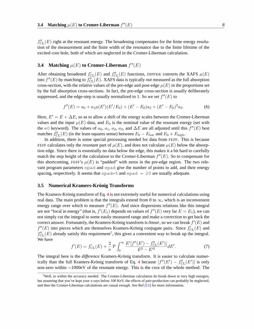
f ′′CL(E) right at the resonant energy. The broadening compensates for the finite energy resolu-tion of the measurement and the finite width of the resonance due to the finite lifetime of theexcited core hole, both of which are neglected in the Cromer-Liberman calculation.

3.4 Matchingµ(E) to Cromer-Liberman f ′′(E)

After obtaining broadenedf ′CL(E) andf ′′CL(E) functions,DIFFKK converts the XAFSµ(E)into f ′′(E) by matching tof ′′CL(E). XAFS data is typicallynot measured as the full absorptioncross-section, with the relative values of the pre-edge and post-edgeµ(E) in the proportions setby the full absorption cross-sections. In fact, the pre-edge cross-section is usually deliberatelysuppressed, and the edge-step is usually normalized to 1. So we setf ′′(E) to

f ′′(E) = a0 + a1µ(E′)(E′/E0) + (E′ −E0)a2 + (E′ − E0)2a3. (6)

Here,E′ = E + ∆E, so as to allow a shift of the energy scales between the Cromer-Libermanvalues and the inputµ(E) data, andE0 is the nominal value of the resonant energy (set withthee0 keyword). The values ofa0, a1, a2, a3, and∆E are all adjusted until thisf ′′(E) bestmatchesf ′′CL(E) (in the least-squares sense) betweenE0 − Elow andE0 + Ehigh.

In addition, there is some special processing needed for data fromFEFF. This is becauseFEFFcalculates only theresonantpart ofµ(E), and does not calculateµ(E) below the absorp-tion edge. Since there is essentially no data below the edge, this makes it a bit hard to carefullymatch the step height of the calculation to the Cromer-Libermanf ′′(E). So to compensate forthis shortcoming,FEFF’s µ(E) is “padded” with zeros in the pre-edge region. The two rele-vant program parametersnpad andepad give the number of points to add, and their energyspacing, respectively. It seems thatnpad=5 andepad = 20 are usually adequate.

3.5 Numerical Kramers-Kr onig Transforms

The Kramers-Kronig transform of Eq.4 is not extremely useful for numerical calculations usingreal data. The main problem is that the integrals extend from 0 to∞, which is an inconvenientenergy range over which to measuref ′′(E). And since dispersions relations like this integralare not “local in energy” (that is,f ′(E1) depends on values off ′′(E) very farE = E1), we cannot simply cut the integral to some easily measured range and make a correction to get back thecorrect answer. Fortunately, the Kramers-Kronig transform islinear, so we can breakf ′(E) andf ′′(E) into pieces which are themselves Kramers-Kronig conjugate pairs. Sincef ′CL(E) andf ′′CL(E) already satisfy this requirement2, this gives a convenient way to break up the integral.We have

f ′(E) = f ′CL(E) +2π

P∫ ∞

0

E′[f ′′(E′)− f ′′CL(E′)]E2 −E′2

dE′. (7)

The integral here is thedifferenceKramers-Kronig transform. It is easier to calculate numer-ically than the full Kramers-Kronig transform of Eq.4 because[f ′′(E′) − f ′′CL(E′)] is onlynon-zero within∼1000eV of the resonant energy. This is the crux of the whole method: The

2Well, to within the accuracy needed. The Cromer-Liberman calculation do break down at very high energies,but assuming that you’ve kept your x-rays below 100 KeV, the effects of pair-production can probably be neglected,and then the Cromer-Liberman calculations are causalenough. See Ref [11] for more information.

3.5 Numerical Kramers-Kr onig Transforms 9

Kramers-Kronig transform of the part off ′′(E) due to the local environment gives the part off ′(E) due to the local environment.

The difference Kramers-Kronig integral can be done over a finite energy range, but it is stilla singular integral, so there is some question about the best way to do it numerically. For that,we rely on Ohta and Ishida[12], who compared several numerical methods for Kramers-Kronigtransforms, and recommended using a MacLaurin series approach for both speed and accuracy.In this sense, the integral in Eq.7 can be approximated at each energy valueEi as

f ′(Ei) = f ′CL(Ei) +4(EN −E1)Eiπ(N − 1)

N/2∑k=1

[f ′′(Ek)− f ′′CL(Ek)]E′2 − E2

(8)

wherek = 2j − i−1. In essence, this is a simple Simpson’s rule integration with the sumbeing over every-other point – to getf ′(Ei) for eveni, sum over theodd indicesj of f ′′(Ej).This conveniently avoids the division by zero ati = j, and still provides enough data to beaccurate. It does, however, lead to a few potential problems to watch out for. First, thef ′′(E)data must be sampled at a high enough frequency so that using every other point is sufficientlyaccurate. Fortunately, the rather slow decay of1/(E′2 − E2) helps assure that enough pointsof f ′′(E) actually count significantly inf ′(E) that this shouldn’t be a serious concern for datasampled at 1eV or so. The second problem is that an abrupt step inf ′′(E)−f ′′CL(E), which canhappen ifE0 of the inputµ(E) is not exactly at the Cromer-LibermanE0 for that resonance,can cause “odd-even noise” where the resultingf ′(E) has some small non-smooth variationsbetween adjacent points. This can usually be reduced, if not eliminated, by broadening theCromer-Libermanf ′′(E) andf ′(E), which effectively spreads the discontinuity in the edge-step enough so that it is seen equivalently by both the even and odd indices, and by making surethat the bare atom calculation and inputµ(E) agree onE0 for the resonance.

4 EXAMPLES 10

4 Examples

Now for a couple examples. Both use Cu as the resonant atom. The first uses measured absorp-tion data for Cu metal, which isn’t all that interesting a problem for DAFS, but illustrates the ba-sics of usingDIFFKK. The second example uses axmu.dat file from FEFFfor YBa2Cu3O6.68,which is a problem slightly more appropriate for DAFS. The files mentioned in this chapter areall available from theDIFFKK web page:

http://cars.uchicago.edu/˜newville/dafs/diffkk/

4.1 Example 1: Experimental Data for Metallic Cu

Here is adiffkk.inp for experimentalµ(E) data of metallic Cu. This file (which is calleddk-exp.inp in the distribution), was derived from runningDIFFKK interactively.:

%------------------------%title = Cu XAFS data

out = exp.fpp % output file namexmu = cu_exp.xmu % xmu data file name

isfeff = false % is this a feff xmu.dat?encol = 1 % energy columnmucol = 2 % mu(E) column

iz = 29 % Z of central atome0 = 8977.9700 % edge energy

egrid = 1.0000 % energy gridewidth = 1.5000 % for broadening CL

elow = 200.0000 % \ how far below and aboveehigh = 500.0000 % / the data range to go

%------------------------%

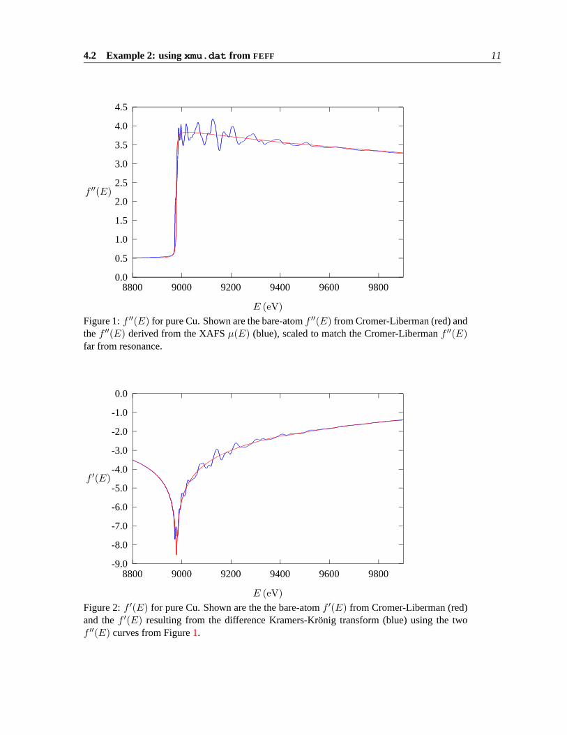
RunningDIFFKK with this input file producesexp.fpp as the output file. Figure1 showsthe f ′′(E) derived from the XAFSµ(E), scaled to match the Cromer-Liberman function farfrom resonance. That would be “the input” toDIFFKK. Figure2 shows “the output” –f ′(E)from the difference Kramers-Kronig transform off ′′(E). the bare-atomf ′′(E) andf ′(E) fromCromer-Liberman are shown for comparison.

4.2 Example 2: usingxmu.dat from FEFF

Now we’ll use axmu.dat file from FEFF with DIFFKK to generate theoreticalf ′(E) andf ′′(E). SinceFEFF calculates the fine-structure of a single atom in a cluster, it can generatethe spectra of an atom at any crystallographic site. XAFS measurements give the average overall atoms in the unit cell. So, in order to model the DAFS for an atom that occupies more thanone site in a unit cell, using experimental XAFS data will not be good enough, and gettingf ′′(E) andf ′(E) from FEFF3 is the only way.

3Well, I suppose youcoulduse some other theoretical XAFS calculation.

4.2 Example 2: usingxmu.dat from FEFF 11

0.0

0.5

1.0

1.5

2.0

2.5

3.0

3.5

4.0

4.5

8800 9000 9200 9400 9600 9800

f ′′(E)

E (eV)Figure 1:f ′′(E) for pure Cu. Shown are the bare-atomf ′′(E) from Cromer-Liberman (red) andthef ′′(E) derived from the XAFSµ(E) (blue), scaled to match the Cromer-Libermanf ′′(E)far from resonance.

-9.0

-8.0

-7.0

-6.0

-5.0

-4.0

-3.0

-2.0

-1.0

0.0

8800 9000 9200 9400 9600 9800

f ′(E)

E (eV)Figure 2:f ′(E) for pure Cu. Shown are the the bare-atomf ′(E) from Cromer-Liberman (red)and thef ′(E) resulting from the difference Kramers-Kronig transform (blue) using the twof ′′(E) curves from Figure1.

4.2 Example 2: usingxmu.dat from FEFF 12

The FEFF calculation here is for the Cu(1) site inYBa2Cu3O6.68. It’s not crucial for thedemonstration here, but the calculation included 78 scattering paths out to 7A. More importantlyfor this application,FEFF7 needed theXANEScard set for it to generate the fullµ(E) (otherwiseit calculates the fine-structureχ without the atomic-like background). Thefeff.inp used togenerate thisxmu.dat is available at theDIFFKK web site.

To generatef ′(E) andf ′′(E), thisdiffkk.inp (which is calleddk-feff.inp in thedistribution) was used:

%------------------------%title = Cu(1) of YBCO

out = feff.fpp % output file namexmu = xmu.dat % xmu file name

isfeff = true % is the a feff xmu.dat?encol = 1 % energy columnmucol = 4 % mu(E) column

iz = 29 % Z of central atome0 = 8986.0700 % edge energy

egrid = 1.0000 % energy gridewidth = 1.5000 % for broadening CL data

elow = 200.0000 % \ how far below and aboveehigh = 500.0000 % / the data range to go

epad = 5.0000 % \ energy grid & # of pointsnpad = 20 % / for pre-padding feff mu(E)

%------------------------%

Running DIFFKK with these settings produced the filefeff.fpp . Figure3 showsf ′′(E)derived fromFEFF’s µ(E), and Figure4 shows thef ′(E) from the difference Kramers-Kronigtransform off ′′(E). The bare-atomf ′′(E) andf ′(E) from Cromer-Liberman are shown forcomparison.

4.2 Example 2: usingxmu.dat from FEFF 13

0.0

0.5

1.0

1.5

2.0

2.5

3.0

3.5

4.0

4.5

8800 9000 9200 9400 9600 9800

f ′′(E)

E (eV)Figure 3:f ′′(E) for the Cu(1) site ofYBa2Cu3O6.68. Shown are the bare-atomf ′′(E) fromCromer-Liberman (red) and thef ′′(E) derived from theµ(E) calculated byFEFF(blue). As forthe experimental data, theFEFF calculation was scaled to match the Cromer-Libermanf ′′(E)far from resonance.

-9.0

-8.0

-7.0

-6.0

-5.0

-4.0

-3.0

-2.0

-1.0

0.0

8800 9000 9200 9400 9600 9800

f ′(E)

E (eV)Figure 4: f ′(E) for the Cu(1) site ofYBa2Cu3O6.68. Shown are the bare-atomf ′(E) fromCromer-Liberman (red) and thef ′(E) from the difference Kramers-Kronig transform (blue).

A DELTAF: BARE ATOM RESONANT SCATTERING FACTORS 14

A DELTAF : bare atom resonant scattering factors

Though the main purpose ofDIFFKK is to “put the XAFS wiggles” on the bare-atom anomalousscattering factors, those bare-atom scattering factors are quite useful on their own. Even forDAFS analysis, it can be very important to include the anomalous scattering factors from non-resonant atoms in order to fully model the intensity. Because of these needs (and because itwas easy to do),DIFFKK is distributed with the companion programDELTAF to generate thebare-atom anomalous scattering factors. This calculation is based completely on the Brennan-Cowan[7] implementation of the Cromer-Liberman[3] work. There are, of course, many similarprograms available.

DELTAF runs in a similar fashion toDIFFKK. First it looks for a filedeltaf.inp . If itfinds this file it reads it and follows the instructions given there. If it can’t finddeltaf.inp ,DELTAF runs interactively, prompting you for the inputs it needs. In either case,deltaf.logwill be written, showing the program parameters used. Anddeltaf.log is in a valid formatfor deltaf.inp . Due to its simpler nature,DELTAF has even fewer parameters thanDIFFKK.A full list is given in Table2.

Table 2:Keywords for DELTAF . The keyword, argument format, meaning, and default valueare listed for each input parameter. The argument format is one of these:char for characterstring, float for floating point number,int for integer, andlog for a logical string (whichcan take valuestrue or false ). Units of energy are in eV.

keyword format meaning default

title char title/comment line noneout char output data file name df.outiz int atomic number for central atom 8elow float lower value for energy range 3000ehigh float upper value of energy range 5000egrid float energy grid for output 1ewidth float energy width for broadening 1.50end - end reading ofdeltaf.inp none

As you can probably tell from this table,DELTAF calculates thef ′(E) andf ′′(E) from theCromer-Liberman tables in a range [elow ,ehigh ] on an energy grid ofegrid . It will applya Lorentzian broadening factor defined byewidth .

B INSTALLATION 15

B Installation

DIFFKK is written in fortran, and should build and install without difficulty on all systemswith a fortran compiler (or a C compiler and f2c). SinceDIFFKK is fairly new, and still un-der some development, it is probably best to get the latest source code from theDIFFKK webpage: http://cars.uchicago.edu/˜newville/dafs/diffkk/. Binary executables for Windows95/NTand Macintosh systems will be made available from the web page as well, but may not be keptas up-to-date as the source. Contact Matt if you need one of these binary versions.

TheDIFFKK source is available as a single (enormous) file or as compressed archive that willuncompress into the code broken apart into subroutines with a Unix-style Makefile. Unix usersshould probably get the compressed archive,difkk.tar.gz , and then follow the “usual”Unix installation:

Unpack the source code:Typegzip -dc diffkk.tar.gz | tar xvf - . This cre-ates a subdirectory diffkksrc, which you should change into (probably by typingcddiffkk src ).

Customize the Makefile: This shouldn’t be necessary, but you may want to edit the Makefileto change the “F77” variable (which tells how to run the fortran compiler and is set to“f77 -O1” by default), and the “INSTALLDIR” variable (which tells where to copy thefiles to if you typemake install , and is set to /usr/local/bin/ by default.)

Build the programs: Typemake. This will create the programsdiffkk anddeltaf .

Compilation of the single-source files should be easier, generally something likef77 -odiffkk diffkk.f , but a little more painful to deal with if anything goes wrong. In eithercase, the compilation of the code for the Cromer-Liberman tables will be fairly slow.

If you have any difficulties compiling or questions about the source code, contact Matt.

REFERENCES 16

References

[1] I. of local structure effects in theoretical x-ray scattering amplitudes using ab-initio x-ray-absorption spectra simulation, Phys. Rev. B58, 11215 (1998).

[2] S. I. Zabinsky et al., Phys. Rev. B 52, 2995 (1995), seehttp://leonardo.phys.washington.edu/feff/.

[3] D. T. Cromer and D. Liberman, J. Chem. Phys.53, 1891 (1970).

[4] L. B. Sorensenet al., in Resonant Anomalous X-Ray Scattering: Theory and Applications,edited by G. Materlik, C. J. Sparks, and K. Fischer (North-Holland, Amsterdam, 1994),pp. 389–420, seehttp://cars.uchicago.edu/˜newville/dafs/icas/.

[5] H. Stragieret al., Phys. Rev. Lett.69, 3064 (1992).

[6] D. H. Templeton, inHandbook of Synchrotron Radiation, edited by G. S. Brown and D. E.Moncton (North-Holland, New York, 1991), Vol. 3, pp. 201–220.

[7] S. Brennan and P. L. Cowan, Rev. Sci. Instrum.63, 850 (1992), seehttp://www-ssrl.slac.stanford.edu/absorb.html.

[8] R. W. James,The Optical Principles of the Diffraction of X-rays(Ox Bow Press, Wood-bridge, CT, 1962).

[9] B. E. Warren,X-ray Diffraction(Dover Publications, Inc, New York, 1969).

[10] J. D. Jackson,Classical Electrodynamics(John Wiley & Sons, New York, 1975).

[11] R. H. Pratt, L. Kissel, and P. M. Bergstrom, Jr., inResonant Anomalous X-Ray Scattering:Theory and Applications, edited by G. Materlik, C. J. Sparks, and K. Fischer (North-Holland, Amsterdam, 1994), pp. 9–33.

[12] K. Ohta and H. Ishida, Applied Spectroscopy42, 952 (1988).

Index

DELTAF, 14diffkk.inp , 2, 3, 7diffkk.log , 2, 5FEFF, 2dk-exp.inp , 10xmu.dat , 2

anomalous scattering,6atomic form factor,6

Cromer-Liberman,2, 7, 14Cu metal,10

DAFS,7

file format,2

interactive session,4

keyworde0 , 3, 5, 8egrid , 3, 7, 14ehigh , 3, 7, 14elow , 3, 7, 14encol , 2, 3epad , 3, 8ewidth , 3, 7, 14isfeff , 2, 3iz , 3, 7, 14mucol , 2, 3npad , 3, 8out , 3, 14title , 3, 14xmudat , 2xmu, 3

Kramers-Kronig,6, 8, 9

Lorentzian broadening,7

MacLaurin series,9

source code,15

Thomson scattering,6

web site,1, 10

zero padding,8