Embed Size (px)
Citation preview

Mathematische Methoden der Unsicherheitsquantifizierung
Oliver Ernst
Professur Numerische Mathematik
Sommersemester 2014
Contents
1 Introduction1.1 What is Uncertainty Quantification?1.2 A Case Study: Radioactive Waste Disposal2 Monte Carlo Methods2.1 Introduction2.2 Basic Monte Carlo Simulation2.3 Improving the Monte Carlo Method2.4 Multilevel Monte Carlo Estimators2.5 The Monte Carlo Finite Element Method3 Random Fields3.1 Introduction3.2 Karhunen-Loève Expansion3.3 Regularity of Random Fields3.4 Covariance Eigenvalue Decay4 Stochastic Collocation4.1 Introduction4.2 Collocation4.3 Analytic Parameter Dependence4.4 ConvergenceOliver Ernst (Numerische Mathematik) UQ Sommersemester 2014 6 / 315

Contents
1 Introduction
2 Monte Carlo Methods
3 Random Fields
4 Stochastic Collocation
Oliver Ernst (Numerische Mathematik) UQ Sommersemester 2014 158 / 315

Contents
1 Introduction
2 Monte Carlo Methods
3 Random Fields
4 Stochastic Collocation4.1 Introduction4.2 Collocation4.3 Analytic Parameter Dependence4.4 Convergence
Oliver Ernst (Numerische Mathematik) UQ Sommersemester 2014 159 / 315
Stochastic CollocationIntroduction
Collocation methods are a long-established technique for solving integral or differ-ential equations and are based on requiring the equation under consideration tohold at a finite number of collocation points sufficient to determine an approximatesolution in an appropriate finite-dimensional function space.
They were introduced for solving PDEs with random inputs in [Xiu & Hesthaven,2005] and [Babuška, Nobile & Tempone, 2007] and offer anumber of atractive features:
Like MC, they reduce to a series of uncoupled deterministic subproblems forwhich legacy code can be used essentialy unmodified.Unlike MC, collocation can take advantage of smooth dependence of thesolution on the random parameters to yield spectral convergence.Nonlinear problems pose no additional difficulty.
Oliver Ernst (Numerische Mathematik) UQ Sommersemester 2014 160 / 315
Stochastic CollocationSetting
We consider the model problem on the bounded domain D Ă Rd
´∇¨pa∇uq “ f on D, u|BD “ 0 (4.1)
with random field data tapx q,x P Du and (possibly) tfpx q,x P Du.
We make the following assumptions:
Assumption 4.1
(a) f P L2pΩ;L2pDqq.(b) a is uniformly bounded from below, i.e., there exists a constant amin ą 0 such
thatapx q ě amin @x P D, P-a.s.
Oliver Ernst (Numerische Mathematik) UQ Sommersemester 2014 161 / 315
Stochastic CollocationSetting
In addition to the space V :“ L2pΩ;H10 pDqq “ L2pΩ;Rq bH1
0 pDq, we introducethe stochastic energy space
Va :“!
v P V : va :“ E“
pa∇v,∇vqL2pDq
‰12ă 8
)
.
Proposition 4.2Under these assumptions Va is continuously embedded in V and
vL2pΩ;H10 pDqq
ď1
aminvVa .
Oliver Ernst (Numerische Mathematik) UQ Sommersemester 2014 162 / 315
Stochastic CollocationStochastic variational problem
With these definitions we give the following variational formulation of problem (4.1)
Find u P Va such that
E“
pa∇u,∇vqL2pDq
‰
“ E“
pf, vqL2pDq
‰
@v P Va. (4.2)
Lemma 4.3
Under Assumption 4.1, the variational problem (4.2) possesses a unique solutionu P Va such that
uL2pΩ;H10 pDqq
ďCDamin
fL2pΩ;L2pDqq,
where CD denotes the Poincaré-Friedrichs constant of D.
Oliver Ernst (Numerische Mathematik) UQ Sommersemester 2014 163 / 315
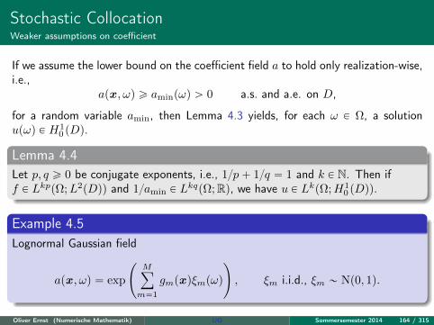
Stochastic CollocationWeaker assumptions on coefficient
If we assume the lower bound on the coefficient field a to hold only realization-wise,i.e.,
apx , ωq ě aminpωq ą 0 a.s. and a.e. on D,
for a random variable amin, then Lemma 4.3 yields, for each ω P Ω, a solutionupωq P H1
0 pDq.
Lemma 4.4Let p, q ě 0 be conjugate exponents, i.e., 1p` 1q “ 1 and k P N. Then iff P LkppΩ;L2pDqq and 1amin P L
kqpΩ;Rq, we have u P LkpΩ;H10 pDqq.
Example 4.5Lognormal Gaussian field
apx , ωq “ exp
˜
Mÿ
m“1
gmpx qξmpωq
¸
, ξm i.i.d., ξm „ Np0, 1q.
Oliver Ernst (Numerische Mathematik) UQ Sommersemester 2014 164 / 315
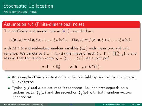
Stochastic CollocationFinite-dimensional noise
Assumption 4.6 (Finite-dimensional noise)The coefficient and source term in (4.1) have the form
apx , ωq “ apx , ξ1pωq, . . . , ξM pωqq, fpx , ωq “ fpx ,x , ξ1pωq, . . . , ξM pωqq
with M P N and real-valued random variables tξmu with mean zero and unitvariance. We denote by Γm “ ξmpΩq the image of each ξm, Γ :“
śMm“1 Γm and
assume that the random vector ξ “ rξ1, . . . , ξM s has a joint pdf
ρ : Γ Ñ R`0 with ρ P L8pΓq.
An example of such a situation is a random field represented as a truncatedKL expansion.Typically f and a are assumed independent, i.e., the first depends on arandom vector ξapωq and the second on ξf pωq with both random vectorsindependent.
Oliver Ernst (Numerische Mathematik) UQ Sommersemester 2014 165 / 315
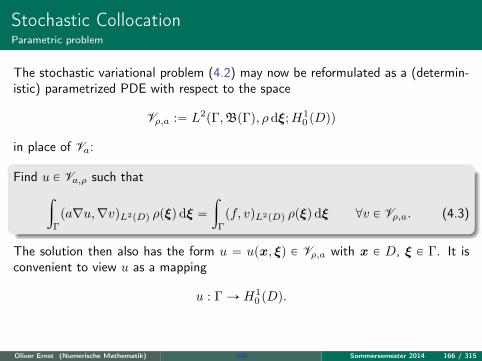
Stochastic CollocationParametric problem
The stochastic variational problem (4.2) may now be reformulated as a (determin-istic) parametrized PDE with respect to the space
Vρ,a :“ L2pΓ,BpΓq, ρdξ;H10 pDqq
in place of Va:
Find u P Va,ρ such thatż
Γ
pa∇u,∇vqL2pDq ρpξqdξ “
ż
Γ
pf, vqL2pDq ρpξqdξ @v P Vρ,a. (4.3)
The solution then also has the form u “ upx , ξq P Vρ,a with x P D, ξ P Γ. It isconvenient to view u as a mapping
u : Γ Ñ H10 pDq.
Oliver Ernst (Numerische Mathematik) UQ Sommersemester 2014 166 / 315

Contents
1 Introduction
2 Monte Carlo Methods
3 Random Fields
4 Stochastic Collocation4.1 Introduction4.2 Collocation4.3 Analytic Parameter Dependence4.4 Convergence
Oliver Ernst (Numerische Mathematik) UQ Sommersemester 2014 167 / 315
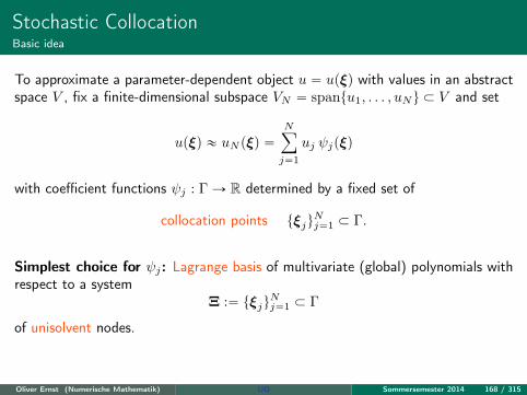
Stochastic CollocationBasic idea
To approximate a parameter-dependent object u “ upξq with values in an abstractspace V , fix a finite-dimensional subspace VN “ spantu1, . . . , uNu Ă V and set
upξq « uN pξq “Nÿ
j“1
uj ψjpξq
with coefficient functions ψj : Γ Ñ R determined by a fixed set of
collocation points tξjuNj“1 Ă Γ.
Simplest choice for ψj: Lagrange basis of multivariate (global) polynomials withrespect to a system
Ξ :“ tξjuNj“1 Ă Γ
of unisolvent nodes.
Oliver Ernst (Numerische Mathematik) UQ Sommersemester 2014 168 / 315
Stochastic CollocationLagrange interpolant
Given a univariate nodal sequence of distinct nodes
χk “ tξpkq1 , . . . , ξpkqnk u, k P N,
we denote by t`pkqj unkj“1 with `pkqj P Pnk´1 the associated Lagrange basis, i.e., the
uniquely determined polynomials of degree nk ´ 1 satisfying
`pkqj pξ
pkqi q “ δi,j , j “ 1, . . . , nk.
We introduce the univariate interpolation operator
Ik : f ÞÑ Ikf “nkÿ
j“1
fpξpkqj q `
pkqj P Pnk´1
Oliver Ernst (Numerische Mathematik) UQ Sommersemester 2014 169 / 315
Stochastic CollocationInterpolation nodes
We will later analyze tensor-product interpolation in the variable ξ and itsapproximation properties, which can be derived from the constituentunivariate interpolations.For univariate interpolation, good nodal sequences are, e.g., zeros oforthogonal polynomials, Clenshaw-Curtiss nodes (extremal values of theChebyshev polynomials) and Leja points.We will restrict ourselves to zeros of orthogonal polynomials. Since these are,at the same time, the nodes of high-order quadrature schemes, this willsimplify the computation of integrals involving the collocation approximation,e.g., to compute moments of the solution of (4.1).
Oliver Ernst (Numerische Mathematik) UQ Sommersemester 2014 170 / 315
Stochastic CollocationTensorized Lagrange interpolant
If we assume Γ is the M -fold Cartesian product of the same (bounded orunbounded) real interval. In this case we may choose the same nodalsequence in all coordinates, and set
Ξk :“ χk ˆ ¨ ¨ ¨ ˆ χk “ tξα “ pξpkqα1, . . . , ξpkqαM q : 1 ď αm ď nku.
Note that N :“ |Ξk| “ nMk .The tensor-product interpolation operator is then defined as
Ik :“ Ik b ¨ ¨ ¨ b Ik : u ÞÑÿ
|α|8ďnk
upξαq `pkqα1¨ . . . ¨ `pkqαM ,
where |α|8 “ maxMm“1 |αm|.The range of the tensor-product interpolation operator Ik is the spaceQnk´1,M of multivariate polynomials of degree nk ´ 1 defined as
Qp,M “
#
Mź
m“1
pmpξmq : pm P Pp
+
.
Oliver Ernst (Numerische Mathematik) UQ Sommersemester 2014 171 / 315
Stochastic CollocationSemi-discrete problem
The semi-discrete problem is obtained by replacing V “ H10 pDq with a
finite-dimensional subspace, say, a finite-element space V h Ă H10 pDq.
If we require the discrete variational problem to hold pointwise in Γ, weobtain the problem
Find uh : Γ Ñ V h such that
papξq∇upξq,∇vqL2pDq “ pfpξq, vqL2pDq @v P V h and @ξ P Γ. (4.4)
Oliver Ernst (Numerische Mathematik) UQ Sommersemester 2014 172 / 315
Stochastic CollocationFully discrete problem
The fully discrete problem is obtained by approximating the semidiscrete solutionuh : Γ Ñ V h by
uhpx , ξq « uh,ppx , ξq :“ pIpuhqpx , ξq,
where Ip is the tensor-product interpolant constructed from univariate Lagrangeinterpolants of degree p, i.e., based on p` 1 disctinct nodes in each variable.
This entails solving a (deterministic) version of (4.1) for each of the tensor-productinterpolation nodes:
Find upξαq P V h for all ξα P Ξ such that
papξαq∇upξαq,∇vqL2pDq “ pfpξαq, vqL2pDq @v P V h. (4.5)
Oliver Ernst (Numerische Mathematik) UQ Sommersemester 2014 173 / 315
Stochastic CollocationAuxiliary density
We have not made the assumption that the random variables tξmuMm“1 areindependent. Expansions containing non-independent random variables arisenaturally when other expansion functions than the covariance eigenfunctionsare employed.Both analysis and computation, however, are considerably simplified whenindependence holds. To this end we introduce an auxiliary density functionρ : Γ Ñ R`0 with the properties
ρpξq “Mź
m“1
ρmpξmq @ξ P Γ and›
›
›
›
ρ
ρ
›
›
›
›
L8pΓq
ă 8. (4.6)
Since the density separates, it can be viewed as the joint pdf of Mindependent random variables.We choose as interpolation nodes the tensor product of univariate nodal setsconsisting of the zeros of the orthogonal polynomials associated with theweight function ρmpξmq in each of the M coordinates ξ1, . . . , ξM .
Oliver Ernst (Numerische Mathematik) UQ Sommersemester 2014 174 / 315

Contents
1 Introduction
2 Monte Carlo Methods
3 Random Fields
4 Stochastic Collocation4.1 Introduction4.2 Collocation4.3 Analytic Parameter Dependence4.4 Convergence
Oliver Ernst (Numerische Mathematik) UQ Sommersemester 2014 175 / 315
Stochastic CollocationWeighted space
Our analysis requires assumptions on f and the densities ρ and ρ:f is a continuous function of ξ which, in case of unbounded parameterdomain Γ, grows at most exponentially at infinity.ρ and ρ behave at infinity like a Gaussian density.
To make these assumptions explicit we introduce a weight function
σpξq :“Mź
m“1
σmpξmq ď 1, σmpξmq “
#
1 if Γm bounded,e´αm|ξm| otherwise,
(4.7)
as well as the function space
CσpΓ;W q :“
"
v : Γ ÑW, v continuous in ξ, maxξPΓ
σpξqvpξqW ă 8
*
where W is a Banach space of functions defined on D.
Oliver Ernst (Numerische Mathematik) UQ Sommersemester 2014 176 / 315
Stochastic CollocationWeighted space
Assumption 4.7 (Growth at infinity)In what follows we assume that(a) f P CσpΓ;L2pDqq and(b) the joint probability density ρ satisfies
ρpξq ď Cρ e´
řMm“1pδmξmq
2
@ξ P Γ (4.8)
for some Cρ ą 0 and δm ą 0 if Γm is unbounded and δm “ 0 otherwise.
Oliver Ernst (Numerische Mathematik) UQ Sommersemester 2014 177 / 315
Stochastic CollocationWeighted space
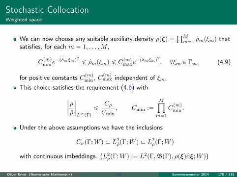
We can now choose any suitable auxiliary density ρpξq “śMm“1 ρmpξmq that
satisfies, for each m “ 1, . . . ,M ,
Cpmqmine
´pδmξmq2
ď ρmpξmq ď Cpmqmaxe´pδmξmq
2
, @ξm P Γm, (4.9)
for positive constants Cpmqmin , Cpmqmax independent of ξm.
This choice satisfies the requirement (4.6) with
›
›
›
›
ρ
ρ
›
›
›
›
L8pΓq
ďCρCmin
, Cmin :“Mź
m“1
Cpmqmin .
Under the above assumptions we have the inclusions
CσpΓ;W q Ă L2ρpΓ;W q Ă L2
ρpΓ;W q
with continuous imbeddings. (L2ρpΓ;W q :“ L2pΓ,BpΓq, ρpξqdξ;W q)
Oliver Ernst (Numerische Mathematik) UQ Sommersemester 2014 178 / 315
Stochastic CollocationWeighted space
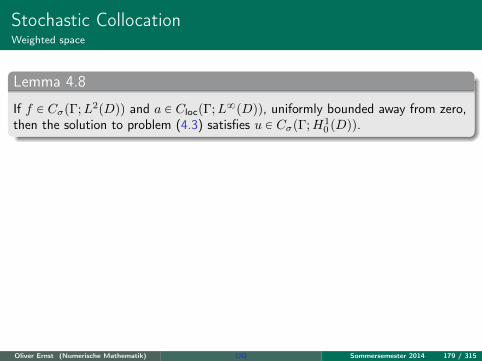
Lemma 4.8
If f P CσpΓ;L2pDqq and a P ClocpΓ;L8pDqq, uniformly bounded away from zero,then the solution to problem (4.3) satisfies u P CσpΓ;H1
0 pDqq.
Oliver Ernst (Numerische Mathematik) UQ Sommersemester 2014 179 / 315
Stochastic CollocationAnalytic extension
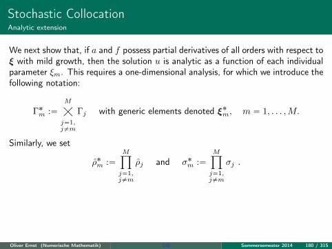
We next show that, if a and f possess partial derivatives of all orders with respect toξ with mild growth, then the solution u is analytic as a function of each individualparameter ξm. This requires a one-dimensional analysis, for which we introduce thefollowing notation:
Γ˚m :“Mą
j“1,j‰m
Γj with generic elements denoted ξ˚m, m “ 1, . . . ,M.
Similarly, we set
ρ˚m :“Mź
j“1,j‰m
ρj and σ˚m :“Mź
j“1,j‰m
σj .
Oliver Ernst (Numerische Mathematik) UQ Sommersemester 2014 180 / 315
Stochastic CollocationAnalytic extension
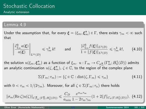
Lemma 4.9
Under the assumption that, for every ξ “ pξm, ξ˚mq P Γ, there exists γm ă 8 such
that›
›
›
›
›
Bkξmapξq
apξq
›
›
›
›
›
L8pDq
ď γkm k! andBkξmfpξqL2pDq
1` fpξqL2pDqď γkm k!, (4.10)
the solution upξm, ξ˚mq as a function of ξm. u : Γm Ñ Cσ˚mpΓ˚m;H1
0 pDqq admitsan analytic continuation upζ, ξ˚mq, ζ P C, to the region of the complex plane
ΣpΓm; τmq :“ tζ P C : distpζ,Γmq ď τmu (4.11)
with 0 ă τm ă 1p2γmq. Moreover, for all ζ P ΣpΓm; τnq there holds
σmpRe ζqupζqC˚σm pΓ˚m;H1
0 pDqqď
CDamin
eαmτm
1´ 2τmγmp1` 2fCσpΓ;H1
0 pDqqq. (4.12)
Oliver Ernst (Numerische Mathematik) UQ Sommersemester 2014 181 / 315
Stochastic CollocationAnalytic extension, examples
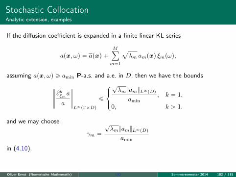
If the diffusion coefficient is expanded in a finite linear KL series
apx , ωq “ apx q `Mÿ
m“1
a
λm ampx q ξmpωq,
assuming apx , ωq ě amin P-a.s. and a.e. in D, then we have the bounds
›
›
›
›
›
Bkξma
a
›
›
›
›
›
L8pΓˆDq
ď
$
&
%
?λmamL8pDq
amin, k “ 1,
0, k ą 1.
and we may choose
γm “
?λmamL8pDq
amin
in (4.10).
Oliver Ernst (Numerische Mathematik) UQ Sommersemester 2014 182 / 315
Stochastic CollocationAnalytic extension, examples
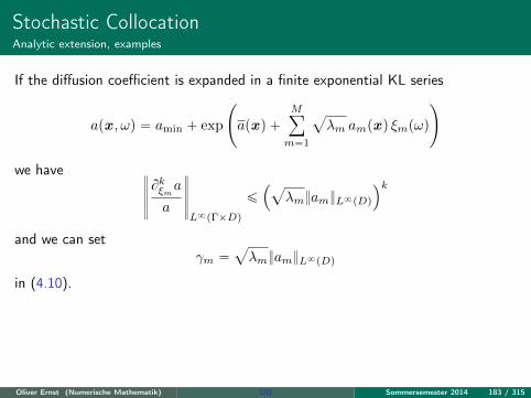
If the diffusion coefficient is expanded in a finite exponential KL series
apx , ωq “ amin ` exp
˜
apx q `Mÿ
m“1
a
λm ampx q ξmpωq
¸
we have›
›
›
›
›
Bkξma
a
›
›
›
›
›
L8pΓˆDq
ď
´
a
λmamL8pDq
¯k
and we can setγm “
a
λmamL8pDq
in (4.10).
Oliver Ernst (Numerische Mathematik) UQ Sommersemester 2014 183 / 315
Stochastic CollocationAnalytic extension, examples
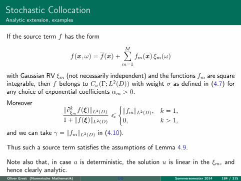
If the source term f has the form
fpx , ωq “ fpx q `Mÿ
m“1
fmpx q ξmpωq
with Gaussian RV ξm (not necessarily independent) and the functions fm are squareintegrable, then f belongs to CσpΓ;L2pDqq with weight σ as defined in (4.7) forany choice of exponential coefficients αm ą 0.
MoreoverBkξmfpξqL2pDq
1` fpξqL2pDqď
#
fmL2pDq, k “ 1,
0, k ą 1,
and we can take γ “ fmL2pDq in (4.10).
Thus such a source term satisfies the assumptions of Lemma 4.9.
Note also that, in case a is deterministic, the solution u is linear in the ξm, andhence clearly analytic.Oliver Ernst (Numerische Mathematik) UQ Sommersemester 2014 184 / 315

Contents
1 Introduction
2 Monte Carlo Methods
3 Random Fields
4 Stochastic Collocation4.1 Introduction4.2 Collocation4.3 Analytic Parameter Dependence4.4 Convergence
Oliver Ernst (Numerische Mathematik) UQ Sommersemester 2014 185 / 315
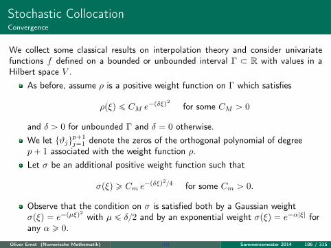
Stochastic CollocationConvergence
We collect some classical results on interpolation theory and consider univariatefunctions f defined on a bounded or unbounded interval Γ Ă R with values in aHilbert space V .
As before, assume ρ is a positive weight function on Γ which satisfies
ρpξq ď CM e´pδξq2
for some CM ą 0
and δ ą 0 for unbounded Γ and δ “ 0 otherwise.We let tϑju
p`1j“1 denote the zeros of the orthogonal polynomial of degree
p` 1 associated with the weight function ρ.Let σ be an additional positive weight function such that
σpξq ě Cm e´pδξq24 for some Cm ą 0.
Observe that the condition on σ is satisfied both by a Gaussian weightσpξq “ e´pµξq
2
with µ ď δ2 and by an exponential weight σpξq “ e´α|ξ| forany α ě 0.
Oliver Ernst (Numerische Mathematik) UQ Sommersemester 2014 186 / 315
Stochastic CollocationConvergence
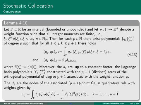
Lemma 4.10Let Γ Ă R be an interval (bounded or unbounded) and let ρ : Γ Ñ R` denote aweight function such that all integer moments are finite, i.e.,ş
Γξn ρpξqdξ ă 8, n P N0. Then for each p P N there exist polynomials tqju
p`1j“1
of degree p such that for all 1 ď j, k ď p` 1 there holds
pqj , qkqρ :“
ż
Γ
qmpξqqnpξq ρpξqdξ “ δj,k,
and pqj , qkqρ “ ϑjδj,k,n,
(4.13)
where ρpξq :“ ξρpξq. Moreover, the qj are, up to a constant factor, the Lagrangebasis polynomials t`ju
p`1j“1 constructed with the p` 1 (distinct) zeros of the
orthogonal polynomial of degree p` 1 associated with the weight function ρ.
The ϑj are the nodes of the associated pp` 1q-point Gauss quadrature rule withweights given by
ωj “
ż
Γ
`jpξqρpξqdξ “
ż
Γ
`jpξq2ρpξqdξ, j “ 1, . . . , p` 1.
Oliver Ernst (Numerische Mathematik) UQ Sommersemester 2014 187 / 315
Stochastic CollocationConvergence
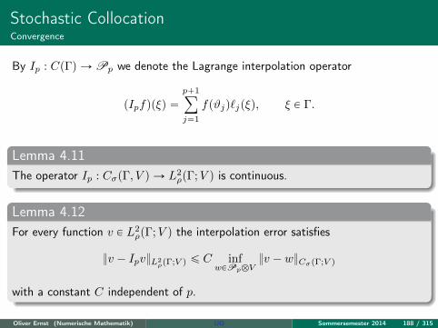
By Ip : CpΓq ÑPp we denote the Lagrange interpolation operator
pIpfqpξq “p`1ÿ
j“1
fpϑjq`jpξq, ξ P Γ.
Lemma 4.11The operator Ip : CσpΓ, V q Ñ L2
ρpΓ;V q is continuous.
Lemma 4.12For every function v P L2
ρpΓ;V q the interpolation error satisfies
v ´ IpvL2ρpΓ;V q ď C inf
wPPpbVv ´ wCσpΓ;V q
with a constant C independent of p.
Oliver Ernst (Numerische Mathematik) UQ Sommersemester 2014 188 / 315
Stochastic CollocationConvergence
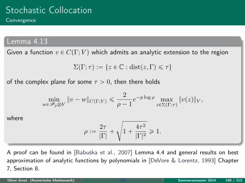
Lemma 4.13Given a function v P CpΓ;V q which admits an analytic extension to the region
ΣpΓ; τq :“ tz P C : distpz,Γq ď τu
of the complex plane for some τ ą 0, then there holds
minwPPpbV
v ´ wCpΓ;V q ď2
ρ´ 1e´p log ρ max
zPΣpΓ;τqvpzqV ,
where
ρ :“2τ
|Γ|`
d
1`4τ2
|Γ|2ě 1.
A proof can be found in [Babuška et al., 2007] Lemma 4.4 and general results on bestapproximation of analytic functions by polynomials in [DeVore & Lorentz, 1993] Chapter7, Section 8.
Oliver Ernst (Numerische Mathematik) UQ Sommersemester 2014 189 / 315
Stochastic CollocationConvergence
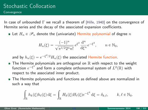
In case of unbounded Γ we recall a theorem of [Hille, 1940] on the convergence ofHermite series and the decay of the associated expansion coefficients.
Let Hn P Pn denote the (univariate) Hermite polynomial of degree n
Hnpξq “p´1qn
?π122nn!
eξ2 dn
dξne´ξ
2
, n P N0,
and by hnpξq “ e´ξ22Hnpξq the associated Hermite function.
The Hermite polynomials are orthogonal on R with respect to the weightfunction e´ξ
2
and form a complete orthonormal system of L2pRq withrespect to the associated inner product.The Hermite polynomials and functions as defined above are normalized insuch a way that
ż
Rhkpξqh`pξqdξ “
ż
RHkpξqH`pξqe
´ξ2 dξ “ δk,`, k, ` P N0.
Oliver Ernst (Numerische Mathematik) UQ Sommersemester 2014 190 / 315
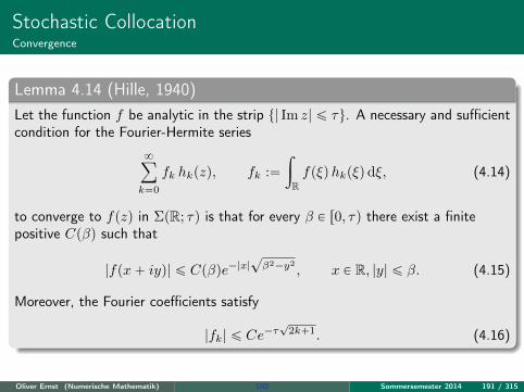
Stochastic CollocationConvergence
Lemma 4.14 (Hille, 1940)Let the function f be analytic in the strip t| Im z| ď τu. A necessary and sufficientcondition for the Fourier-Hermite series
8ÿ
k“0
fk hkpzq, fk :“
ż
Rfpξqhkpξqdξ, (4.14)
to converge to fpzq in ΣpR; τq is that for every β P r0, τq there exist a finitepositive Cpβq such that
|fpx` iyq| ď Cpβqe´|x|?β2´y2 , x P R, |y| ď β. (4.15)
Moreover, the Fourier coefficients satisfy
|fk| ď Ce´τ?
2k`1. (4.16)
Oliver Ernst (Numerische Mathematik) UQ Sommersemester 2014 191 / 315
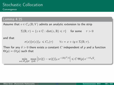
Stochastic CollocationConvergence
Lemma 4.15Assume that v P CσpR;V q admits an analytic extension to the strip
ΣpR; τq “ tz P C : distpz,Rq ď τu for some τ ą 0
and thatσpxqvpzqV ď Cvpτq @z “ x` iy P ΣpR; τq.
Then for any δ ą 0 there exists a constant C independent of p and a functionΘppq “ Oppq such that
minwPPpbV
maxξPR
ˇ
ˇ
ˇvpξq ´ wpξqV e
´pδξq24ˇ
ˇ
ˇď C Θppq e´τδ
?p.
Oliver Ernst (Numerische Mathematik) UQ Sommersemester 2014 192 / 315
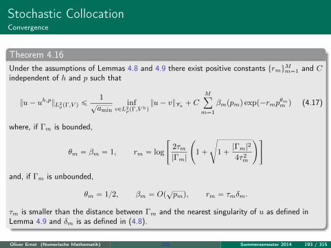
Stochastic CollocationConvergence
Theorem 4.16Under the assumptions of Lemmas 4.8 and 4.9 there exist positive constants trmuMm“1 and Cindependent of h and p such that
u´ uh,pL2ρpΓ,V q
ď1
?amin
infvPL2
ρpΓ,Vhqu´ vVa ` C
Mÿ
m“1
βmppmq expp´rmpθmm q (4.17)
where, if Γm is bounded,
θm “ βm “ 1, rm “ log
«
2τm|Γm|
˜
1`
d
1`|Γm|2
4τ2m
¸ff
and, if Γm is unbounded,
θm “ 12, βm “ Op?pmq, rm “ τmδm.
τm is smaller than the distance between Γm and the nearest singularity of u as defined inLemma 4.9 and δm is as defined in (4.8).
Oliver Ernst (Numerische Mathematik) UQ Sommersemester 2014 193 / 315