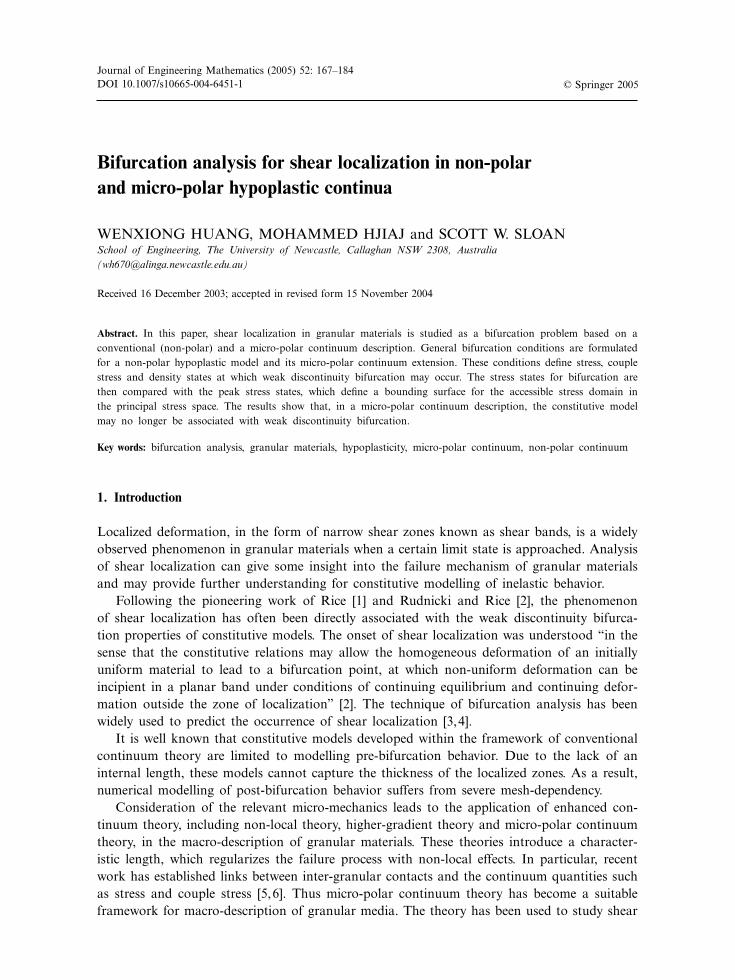
DOI 10.1007/s10665-004-6451-1Journal of Engineering Mathematics (2005) 52: 167–184

© Springer 2005

Bifurcation analysis for shear localization in non-polarand micro-polar hypoplastic continua

WENXIONG HUANG, MOHAMMED HJIAJ and SCOTT W. SLOANSchool of Engineering, The University of Newcastle, Callaghan NSW 2308, Australia(wh670@alinga.newcastle.edu.au)

Received 16 December 2003; accepted in revised form 15 November 2004

Abstract. In this paper, shear localization in granular materials is studied as a bifurcation problem based on aconventional (non-polar) and a micro-polar continuum description. General bifurcation conditions are formulatedfor a non-polar hypoplastic model and its micro-polar continuum extension. These conditions define stress, couplestress and density states at which weak discontinuity bifurcation may occur. The stress states for bifurcation arethen compared with the peak stress states, which define a bounding surface for the accessible stress domain inthe principal stress space. The results show that, in a micro-polar continuum description, the constitutive modelmay no longer be associated with weak discontinuity bifurcation.

Key words: bifurcation analysis, granular materials, hypoplasticity, micro-polar continuum, non-polar continuum

1. Introduction

Localized deformation, in the form of narrow shear zones known as shear bands, is a widelyobserved phenomenon in granular materials when a certain limit state is approached. Analysisof shear localization can give some insight into the failure mechanism of granular materialsand may provide further understanding for constitutive modelling of inelastic behavior.

Following the pioneering work of Rice [1] and Rudnicki and Rice [2], the phenomenonof shear localization has often been directly associated with the weak discontinuity bifurca-tion properties of constitutive models. The onset of shear localization was understood “in thesense that the constitutive relations may allow the homogeneous deformation of an initiallyuniform material to lead to a bifurcation point, at which non-uniform deformation can beincipient in a planar band under conditions of continuing equilibrium and continuing defor-mation outside the zone of localization” [2]. The technique of bifurcation analysis has beenwidely used to predict the occurrence of shear localization [3,4].

It is well known that constitutive models developed within the framework of conventionalcontinuum theory are limited to modelling pre-bifurcation behavior. Due to the lack of aninternal length, these models cannot capture the thickness of the localized zones. As a result,numerical modelling of post-bifurcation behavior suffers from severe mesh-dependency.

Consideration of the relevant micro-mechanics leads to the application of enhanced con-tinuum theory, including non-local theory, higher-gradient theory and micro-polar continuumtheory, in the macro-description of granular materials. These theories introduce a character-istic length, which regularizes the failure process with non-local effects. In particular, recentwork has established links between inter-granular contacts and the continuum quantities suchas stress and couple stress [5,6]. Thus micro-polar continuum theory has become a suitableframework for macro-description of granular media. The theory has been used to study shear

168 W. Huang et al.

localization in granular materials by Muhlhaus [7], de Borst [8], Dietsche et al. [9] and Ehlersand Volk [10] who adopted an elastoplastic approach, and by Tejchman [11], Tejchman andBauer [12], Bauer and Huang [13], Tejchman and Gudehus [14] and Huang and Bauer [15]who adopted a hypoplastic approach. It is widely accepted that post-bifurcation behavior canbe well captured by micro-polar continuum models. Numerical results for shearing of a gran-ular layer between two parallel plates show that a localized shear zone of finite thickness canbe obtained, which is mesh-independent provided that the element size is small enough [14,15].

An open question with the micro-polar continuum description of granular materials iswhether shear localization will occur in a homogeneous deforming specimen in the form ofweak discontinuity bifurcation (as is the case in a conventional continuum description). Thispaper focuses on bifurcation analysis of constitutive models developed for cohesionless granu-lar materials using a conventional (non-polar) continuum approach and a micro-polar contin-uum approach. The non-polar hypoplastic model proposed by Gudehus [16] and Bauer [17],and its micro-polar continuum extension formulated by Huang et al. [18], are employed forthis purpose. In these non-polar and micro-polar models, the void ratio is incorporated asa measurement of density. This allows the stationary state (the so-called critical state) to bedescribed and the pressure- and density-dependent behavior to be captured for a wide rangeof stress and density levels with a single set of constitutive constants.

Hypoplastic constitutive models belong to a category known as incrementally nonlinearmodels. Bifurcation analysis of non-polar models of this type was first discussed by Kolym-bas [19] and Chambon and Desrues [20]. A more general analysis can be found in [21,22].Bauer and Huang [23] and Bauer [24] discussed the pressure and density effects in bifurca-tion and shear localization. Wu and Sikora [25] and Wu [26] presented a bifurcation surfacein principal-stress space for a density-independent hypoplastic model. Fewer results are knownfor bifurcation analysis of micro-polar continuum models. Some early results can be found in,for instance, [9,27].

In this paper, a general criterion for bifurcation is first derived for the non-polarhypoplastic continuum. By extending the concept of a weak discontinuity in the micro-polarcontinuum, a similar bifurcation criterion is formulated for the micro-polar hypoplastic con-tinuum. In order to assess the possibility of shear bifurcation in a general way, a conditionfor the peak stress state is provided. Geometric representations of the bifurcation states andpeak stress states in the deviatoric stress plane are then presented, from which the accessibilityof bifurcation points can be determined.

Symbolic notation is used for vectors and tensors in this paper. Vectors and second-ordertensors are distinguished by bold-faced font and fourth-order tensors by calligraphic font.Index notation is used by referring to a fixed orthogonal Cartesian coordinate system. Thesecond-order unit tensor and the fourth-order unit tensor are denoted by I and I, respec-tively. Their components read (I)ij = δij and (I)ijkl = δikδjl with δij being the Kroneckerdelta. The permutation symbol ε is used with (ε)ijk = 1 for ijk ∈ {{1,2,3}, {2,3,1}, {3,1,2}},(ε)ijk = −1 for ijk ∈ {{1,3,2}, {2,1,3}, {3,2,1}} and (ε)ijk = 0 otherwise. The dot-productoperation is used for a · b = aibi , (A · b)i = Aijbj , A : B = AijBij and (A : B)ij = AijklBkl .Here, the usual summation convention for dummy indices is adopted. Dyadic multiplica-tion is denoted by the symbol ⊗. For instance (a ⊗ b)ij = aibj and (A ⊗ B)ijkl = AijBkl .The Euclidean norm is used for all vectors so that ‖a‖ = √a ·a and all tensors so that‖A‖ = √A : A. The Nabla operator ∇ is so defined that (∇a)ij = ∂ai/∂xj and (∇ · a) =∂ai/∂xi .

Bifurcation analysis for shear localization 169

2. Hypoplastic description of granular materials

2.1. Outline of the micro-polar continuum

A micro-polar continuum is characterized by additional rotational degrees of freedom andthe presence of a couple stress which is work-conjugated with the micro-curvature (associatedwith the rotational degrees of freedom). Material particles in a micro-polar continuum cantranslate and rotate independently. Here we use the vectors u and wc to denote the rate oftranslation (velocity) and the rate of rotation (angular velocity) of material particles. Then thedeformation rate of a micro-polar (Cosserat) continuum can be measured by the strain rateεc and the micro-curvature rate κ , which are defined by the following kinematic relations:

εc=∇u+ ε · wc, εcij = ∂ui/∂xj + εijkwck, (1a)

κ=∇wc, κij = ∂wci /∂xj . (1b)

By introducing the notion of micro-spin ωc=−ε · wc, Equation (1a) can also be written in theform of:

εc= ε+ ω− ωc,

where ε= d= 12 [∇u+ (∇u)T ] and ω= 1

2 [∇u− (∇u)T ], the symmetric part and the skew sym-metric part of the velocity gradient, are the strain rate and the spin (termed the macro spinin this paper) for the non-polar continuum. The strain rate for the micro-polar continuum εc

is generally non-symmetric. In the case where the micro-spin coincides with the macro-spin,it becomes symmetric and coincides with the strain rate for the non-polar continuum.

The equilibrium equations for a micro-polar continuum must take into account the pres-ence of the couple stress µ. In cases where body forces and body couples are absent, the localform of the equilibrium equations read:

∇ ·σ T =0, ∂σij /∂xj =0, (2a)

∇ ·µT − ε :σ =0, ∂µij /∂xj − εijkσjk=0. (2b)

From the second equation, we see that the stress tensor is generally non-symmetric for amicro-polar continuum. When the couple stress vanishes, the stress tensor becomes symmetric.

2.2. Hypoplastic model for non-polar and micro-polar continuum

In hypoplasticity, the granular material is described as a continuum in terms of material stateand material properties. The latter are represented by constitutive constants which do notchange during loading. In a non-polar (conventional) continuum approach, the material stateis characterized by the current stress σ and the void ratio e, while in a micro-polar continuumdescription the couple stress µ is also included.

In the nonpolar continuum description, a practical hypoplastic constitutive equation forthe cohesionless granular materials has the following general form [16]:

σ =fs(L(σ ) : ε+fdN(σ )‖ε‖). (3)

The objective time rate of the Cauchy stress, σ , is a nonlinear function of the strain rate ε.Herein the fourth-order tensor L and the second-order tensor N are functions of the normal-ized stress σ = σ/tr σ , and the scalar factors fs and fd (known as the stiffness factor andthe density factor, respectively) are functions of the mean pressure p=−tr σ/3 and the void

170 W. Huang et al.

ratio e. The elaborated nonlinear tensor-valued function allows the description of differentstiffness for loading and unloading without employing the elastoplastic concept of decompo-sition of strain rate into an elastic part and a plastic part. As σ is a positively homogeneousof order one in ε, the rate-independent behavior is described by (3).

In a micropolar continuum extension [18] of constitutive equation (3), the objective timerate of the stress, σ , and the objective time rate of couple stress, µ , are expressed as

σ =fs[Lσσ : εc+Lσµ : κ∗ +fdNσR], (4a)

µ=d50fs[Lµµ : κ∗ +Lµσ : εc+fdNµR], (4b)

where d50 denotes the mean grain diameter, which is a natural length scale for granular mate-rials, κ∗=d50κ is the scaled micro-curvature rate, and R is a combination of the norms of thestrain rate and the micro-curvature rate in the form of

R=√

ε : ε+ δ2κ : κ, (5)

where

δ= (aµ/a)d50 (6)

is a characteristic length which scales the thickness of shear bands. The fourth-order tensorsand the second-order tensors depend on the normalized stress tensor, σ , and the normalizedcouple-stress tensor, µ=µ/(d50tr σ ), with the following representations:

Lσσ = a2I+ σ ⊗ σ , Lσµ= σ ⊗ µ, Nσ = a(σ + σd),

Lµµ =a2µI+ µ⊗ µ, Lµσ = µ⊗ σ , Nµ=2aµ.

(7)

Herein σd = σ − I/3 denotes the deviator of the normalized stress, and a and aµ are two

parameters related to the limit value of stress and couple stress at stationary states.A stationary state is reached when there is no change in the state variables under contin-

uing deformation. The present micro-polar hypoplastic model is characterized by the follow-ing limit condition on the stress, the couple stress, and the void ratio at stationary states [18]:

‖σ d‖2

a2+ ‖µ‖

2

a2µ

=1 and fd=1. (8)

This relation shows a coupling between the limit stress and the limit couple stress. It also pro-vides a physical interpretation for the parameters a and aµ.

The evolution of the void ratio is governed by the equation:

e= (1+ e)tr ε, (9)

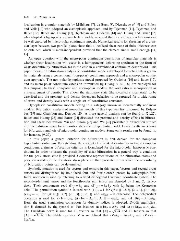
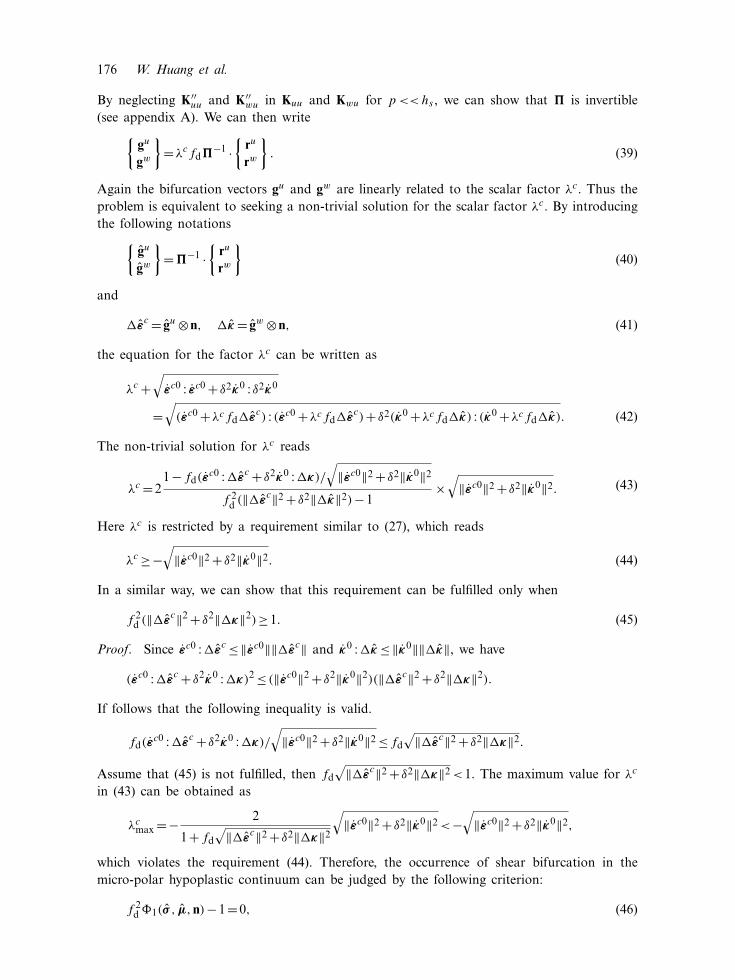
which is a result of mass balance by neglecting the volume change in solid grains. The voidratio of a granular material is bounded by the maximum void ratio ei for the loosest statesand the minimum void ratio ed for the densest state, and it tends to a critical void ratio ec atstationary states. ei , ed and ec are pressure-dependent quantities. In the present model, thevariation of ei , ed and ec with the mean pressure p is described by the following relation(refer to Figure 1):

ec

eco= ed

edo= ei

eio= exp{(3p/hs)n}. (10)

Bifurcation analysis for shear localization 171

Figure 1. Pressure dependence of the maximum,the critic and the minimum void ratio [17].

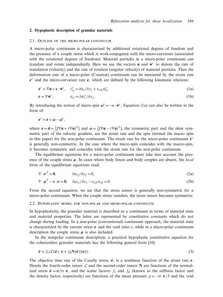
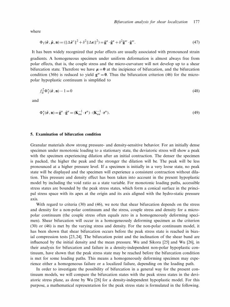
Figure 2. Sketch of weak discontinuity plane in theprincipal stress space.

Herein hs and n are two material constants that determine the shape of the void ratio-pressure curves, and eio, edo and eco are three material constants which represent the maxi-mum, minimum and critical void ratio at the stress-free state. The density factor fd is relatedto the pressure-dependent relative density according to

fd=(e− ed

ec− ed

)α, (11)

where α is a material constant which scales the peak stress state under loading. Note thatdilative deformation corresponds to an increase in the value for fd. The densest state is char-acterized by fd = 0, while fd = 1 corresponds to e= ec. Therefore, the critical void ratio isreached at a stationary state, which is in accordance with experimental observations for gran-ular materials.

The stiffness factor fs has the following representation:

fs= hs

n(σ : σ )

(eie

)β 1+ ei

ei

(p

hs

)(1−n)[3a2

i +1+√

3aifdi ]−1. (12)

Herein fdi and ai represent the values of fd and a at isotropic states. From (10) and (11),fdi has a constant value fdi ={(eio− edo)/(eco− edo)}α. As described later, ai has a constantvalue, which is related to the critical friction angle φc. The term (ei/e)

β reflects the influenceof the density on the stiffness factor with β≈1 being another material constant.

For the special case where the couple stress and micro-curvature rate vanish and themicro-spin coincides with the macro-spin, the non-polar continuum model proposed by Gude-hus [16] and Bauer [17] is recovered with

Lσσ =L= a2I+ σ ⊗ σ , Nσ =N= a(σ + σd). (13)

Correspondingly, the limit stress at a stationary state satisfies the following condition:

||σ d ||= a, (14)

which represents a conical surface in the principal stress space with its apex at the origin.Bauer [28] showed that it is possible to embed different limit stress conditions into this model

172 W. Huang et al.

by adopting different expressions for the parameter a. For instance, a constant value for a

corresponds to a Drucker–Prage type limit condition. With the following formulation, theMatsuoka–Nakai limit condition is embedded:

a= sinϕc3− sinϕc

⎡⎣√√√√8/3−3||σ sd ||2+√3/2||σ sd ||3 cos(3θ)

1+√3/2||σ sd || cos(3θ)−||σ sd ||

⎤⎦ , (15)

where σsd denotes the deviator of the normalized symmetric stress, and θ denotes the Lode

angle defined in the deviatoric stress plane for the symmetric stress.The limit couple stress related parameter aµ is considered to be constant. For a granular

material without preferred grain orientation, this is a reasonable assumption. All the materialconstants in this model, except aµ, can be determined easily from elementary laboratory testsas discussed in detail by Herle and Gudehus [29]. aµ may be determined from a back analy-sis procedure after measuring the shear band thickness, which requires advanced techniques.For the following discussion we note that the stiffness factor fs has a value of the order ofhns p

1−n. The granular hardness (as termed in Gudehus [16]) hs , which has a dimension ofstress, has a typical value of the order of 1·0×106 kPa or higher for sands. The dimensionlessexponent n falls in the range of (0·25,0·5) [29].

3. Bifurcation analysis for the non-polar hypoplastic continuum

Consider a homogeneous specimen under uniform deformation and assume that the velocityand stress fields are continuous up to a certain state where a discontinuity in the velocity gra-dient across a planar surface becomes possible. This weak discontinuity plane S is then char-acterized by the following kinematic conditions:

[[l]]= [[∇u]]= (∇u)1− (∇u)0=g⊗n and [[u]]= u1− u0=0. (16)

Here the superscript 0 and 1 are used to denote the values for a quantity on either side ofthe discontinuity plane. Equation (16) states that across the discontinuous plane S the veloc-ity gradient is experiencing a jump, which is characterized by a vector g and the unit normalvector n to the discontinuity plane, while the velocity field itself is continuous. Correspond-ing to the discontinuous velocity gradient, jumps in the strain rate and the spin tensor willbe encountered on crossing S:

[[ε]]= ε1− ε0= 12(g⊗n+n⊗n), (17a)

[[ω]]= ω1− ω0= 12(g⊗n−n⊗g). (17b)

In response to this, the stress rate becomes discontinuous. A bifurcation condition can be for-mulated by considering rate-form equilibrium long the possible discontinuity plane. Concern-ing the fact that the direction of the discontinuity plane varies with time due to the motion,we start to consider the equilibrium in a reference configuration (A reference configuration isa fixed configuration in the space which uniquely designates a one-to-one mapping with mate-rial points in motion.). On the image discontinuity plane in the reference configuration, thenominal traction rate must be unique, i.e., [[P]] ·N= 0, where P is the first Piola–Kirchhoffstress and N is the unit normal of the image discontinuity plane, which is independent of time.Using the well-known relation P=Jσ ·F−T and the Nanson’s formula (see, for instance, [30,

Bifurcation analysis for shear localization 173

p. 75]) the following equation is obtained:

[[σ + (div u)σ −σ · lT ]] ·n= [[σ ]] ·n+ ([[div u]]σ −σ · [[lT ]]) ·n=0. (18)

Note that the material response is described in terms of the objective time rates of stress andcouple stress. There is an infinite number of possibilities which define an objective time ratefor the stress tensor. The most widely used objective stress rates include the Zaremba–Jau-mann rate, the Oldroyd rate, the Green–Naghdi rate and the Truesdell rate ([30, Section5.3]).Choosing a proper objective stress rate is, in many cases, a problem of a proper formulationof the constitutive equations. It should also be noted that the discrepancies due to the choiceof different objective stress rates become significant only when a large shear deformation hastaken place (e.g. [28]). At the beginning of shear localization, such discrepancies are negligi-ble. In this study, we take the Zaremba–Jaumann rate as the objective time rate for both thestress tensor and the couple stress tensor:

σ = σ − (ω ·σ −σ · ω), (19a)

µ= µ− (ω ·µ−µ · ω). (19b)

Substitution of (19a) in (18) yields the following bifurcation condition

[[σ ]] ·n+ ([[div u]]σ ·n+ [[ω]] ·σ ·n−σ · [[d]]) ·n=0. (20)

Invoking the constitutive relations leads to the following equations for the components of thevector g:

K ·g−λfdr=0. (21)

The following notations are introduced in this equation: the scalar factor λ=||ε1||−||ε0||, thevector r=−a(σ + σ

d) ·n and the tensor K=K′ +K′′, where

K′ = a2

2 (I+n⊗n)+ (σ ·n)⊗ (σ ·n),K′′ = − 3p

fs[σ ·n⊗n−n⊗n · σ T ].

(22)

In the representation for K′′, the factor −3p comes out from the stress normalization. Sincethe stiffness factor fs ∼ hns p

1−n, it follows that the factor p/fs has a value of the order of(p/hs)

n. Therefore, for most practical stress states with p<<hs , K′ is the dominant term inK and K′′ can be neglected. Because K′ is positive-definite and therefore invertible, K is alsoinvertible. Then we can write g as a linear function of the scalar factor λ:

g=λfdK−1 · r. (23)

For λ=0, we have only a null solution for g, which indicates no bifurcation at all. Thus thebifurcation problem is equivalent to seeking a non-trivial solution for the scalar factor λ. Byintroducing the notations

g=K−1 · r and ε= 12(g⊗n+n⊗ g), (24)

we can write the strain rate as ε1= ε0+λfdε. It follows that the nonlinear equation for thescalar factor λ can be written as

λ−(√

(ε0+λfdε) : (ε0+λfdε)−√

ε0 : ε0)=0. (25)

174 W. Huang et al.

Algebraic manipulation leads to the following equation:

(f 2dε :ε−1))λ2+2(fdε0 :ε−‖ε0‖)λ=0.

The non-trivial solution for λ then reads

λ=2‖ε0‖−fdε0 :ε

f 2dε :ε−1

=21−fd‖ε‖ cosγ

f 2dε :ε−1

‖ε0‖ (26)

with cosγ := (ε0 :ε)/(‖ε0‖‖ε‖). Note that λ is restricted by the condition

λ≥−‖ε0‖, (27)

since ‖ε‖=λ+‖ε0‖≥0. It can be shown that the requirement (27) can be fulfilled only when

f 2dε :ε= f 2

d

2[g · g+ (g ·n)2]≥1. (28)

Proof. Assume that (28) is not fulfilled, then fd‖ε‖<1. The maximum value for λ in (26)corresponds to cosγ =1, which reads

λmax=− 21+fd‖ε‖‖ε

0‖<−‖ε0‖, (29)

which violates the requirement (27).

Remark . Inequality (28) can also be obtained in an alternative way. Note that a triangularinequality ‖ε1 − ε0‖2 ≥ (‖ε1‖− ‖ε0‖)2 is generally valid. Substitution of (‖ε1‖− ‖ε0‖)2 = λ2

and ‖ε1 − ε0‖2 = λ2f 2d (g · g+ (g · n)2)/2 leads to inequality (28). This approach is simpler.

However, the approach from (25) to (28) provides more detail about the factor λ and can berepeated for derivation of the bifurcation criterion for the micro-polar continuum model.

Remark . The equality in (28) corresponds to either ||ε1||/||ε0||=∞ or cosγ =1. The later istrue only when ε1 is co-axial with ε0, which corresponds to pure dilation or contraction inthe localized zone. For a uniformly deforming process leading to a continuous onset of shearbifurcation, the equality represents a limit state at which the bifurcation will not occur.

To assess whether the bifurcation condition is met in a loading program, the equality can beused as a determinant. That is, incipience of shear localization is indicated by the followingcondition:

f 2d�0(σ ,n)−1=0, (30)

with

�0(σ ,n)= 12

[g · g+ (g ·n)2]= 12

[(K−1 · r) · (K−1 · r)+ (n ·K−1 · r)2]. (31)

Note that for p<<hs , K′′ can be neglected in the representation of K. In the case where p∼hs or p>hs , we have ei/e∼ 1, which implies that fs and K′′ are almost independent of thevoid ratio. Therefore, in the criterion (30), �0 can be considered independent of the density.The influence of the density on bifurcation is reflected only by the factor fd, which is sepa-rated from �0.

Bifurcation analysis for shear localization 175

4. Bifurcation analysis for the micro-polar hypoplastic continuum

Similar conditions for weak-discontinuity bifurcation can be formulated for a micro-polarhypoplastic continuum. We start again with a homogeneously deforming specimen in whichthe velocity, rotation rate, stress and couple stress fields are continuous up to a state wherea banded planar weak discontinuity may develop. Across the weak discontinuity plane S, thevelocity and the rotation rate fields are initially continuous:

[[u]]= u1− u0=0 and [[wc]]= wc1− wc0=0 , (32)

while the jump in the velocity gradient and the rotation-rate gradient can be written as

[[∇u]]= (∇u)1− (∇u)0=gu⊗n, (33a)

[[κ ]]= (∇wc)1− (∇wc)0=gw⊗n. (33b)

Weak discontinuity bifurcation is characterized by vectors gu,gw and the unit normal vectorn for the discontinuity plane S. With respect to the discontinuity in the velocity gradient, thejumps in the strain rate and in the macro-spin read

[[εc]]= εc1− εc0= [[∇u+ ε ·wc]]=gu⊗n, (34a)

[[ω]]= ω1− ω0= 12(gu⊗n−n⊗gu). (34b)

Similar to the situation for the nonpolar continuum, consideration of the equilibrium in rateform along the discontinuity plane leads to the following conditions to be fulfilled by the totalstress rate and the total couple stress rate:

[[σ ]] ·n+ ([[div u]]σ −σ · [[lT ]]) ·n=0, (35a)

[[µ]] ·n+ ([[div u]]µ−µ · [[lT ]]) ·n =0. (35b)

Using the expressions for stress rate (19a) and couple-stress rate (19b) and the constitutiveEquations (4a) and (4b), the following nonlinear equations are obtained for the vectors gu

and gw:

Kuu ·gu+Kuw ·gw−λcfdru=0, (36a)

Kwu ·gu+Kww ·gw−λcfdrw=0. (36b)

Herein the following notations are used: the scalar factor λc= [[R]], the vectors ru=−a(σ +σd) · n and rw=−2aµ · n, and the tensors Kuu=K′uu+K′′uu,Kuw=K′uw,Kwu=K′wu+K′′wu and

Kww=K′ww with the following representations:

K′uu = a2I+ (σ ·n)⊗ (σ ·n), K′uw=d50(σ ·n)⊗ (µ ·n),K′wu = (µ ·n)⊗ (σ ·n), K′ww=d50[a2

µI+ (µ ·n)⊗ (µ ·n)],K′′uu = − 3p

fs[σ ·n⊗n−n⊗n · σ T ],

K′′wu = − 3pfs

[µ ·n⊗n−n⊗n · µT ].

(37)

For a concise representation, we define � according to

� :=[

Kuu Kuw

Kwu Kww

]. (38)

176 W. Huang et al.

By neglecting K′′uu and K′′wu in Kuu and Kwu for p<<hs , we can show that � is invertible(see appendix A). We can then write{

gu

gw

}=λcfd�−1 ·

{ru

rw

}. (39)

Again the bifurcation vectors gu and gw are linearly related to the scalar factor λc. Thus theproblem is equivalent to seeking a non-trivial solution for the scalar factor λc. By introducingthe following notations{

gu

gw

}=�−1 ·

{ru

rw

}(40)

and

εc= gu⊗n, κ= gw⊗n, (41)

the equation for the factor λc can be written as

λc+√

εc0 : εc0+ δ2κ0 : δ2κ0

=√(εc0+λcfdε

c) : (εc0+λcfdε

c)+ δ2(κ0+λcfdκ) : (κ0+λcfdκ). (42)

The non-trivial solution for λc reads

λc=21−fd(ε

c0 :εc+ δ2κ0 :κ)/

√‖εc0‖2+ δ2‖κ0‖2

f 2d (‖ε

c‖2+ δ2‖κ‖2)−1×√‖εc0‖2+ δ2‖κ0‖2. (43)

Here λc is restricted by a requirement similar to (27), which reads

λc≥−√‖εc0‖2+ δ2‖κ0‖2. (44)

In a similar way, we can show that this requirement can be fulfilled only when

f 2d (‖ε

c‖2+ δ2‖κ‖2)≥1. (45)

Proof. Since εc0 :εc≤‖εc0‖‖ε

c‖ and κ0 :κ≤‖κ0‖‖κ‖, we have

(εc0 :εc+ δ2κ0 :κ)2≤ (‖εc0‖2+ δ2‖κ0‖2)(‖ε

c‖2+ δ2‖κ‖2).

If follows that the following inequality is valid.

fd(εc0 :ε

c+ δ2κ0 :κ)/

√‖εc0‖2+ δ2‖κ0‖2≤fd

√‖ε

c‖2+ δ2‖κ‖2.

Assume that (45) is not fulfilled, then fd√‖ε

c‖2+ δ2‖κ‖2 <1. The maximum value for λc

in (43) can be obtained as

λcmax=−2

1+fd√‖ε

c‖2+ δ2‖κ‖2

√‖εc0‖2+ δ2‖κ0‖2 <−

√‖εc0‖2+ δ2‖κ0‖2,

which violates the requirement (44). Therefore, the occurrence of shear bifurcation in themicro-polar hypoplastic continuum can be judged by the following criterion:

f 2d�1(σ , µ,n)−1=0, (46)

Bifurcation analysis for shear localization 177

where

�1(σ , µ,n)= (‖εc‖2+ δ2‖κ‖2)= gu · gu+ δ2gw · gw. (47)

It has been widely recognized that polar effects are usually associated with pronounced strain

gradients. A homogeneous specimen under uniform deformation is almost always free frompolar effects, that is, the couple stress and the micro-curvature will not develop up to a shearbifurcation state. Therefore we have µ=0 at the incipience of bifurcation, and the bifurcationcondition (36b) is reduced to yield gw=0. Thus the bifurcation criterion (46) for the micro-polar hypoplastic continuum is simplified to

f 2d�

∗1(σ ,n)−1=0 (48)

and

�∗1(σ ,n)= gu · gu= (K−1uu · ru) · (K−1

uu · ru). (49)

5. Examination of bifurcation condition

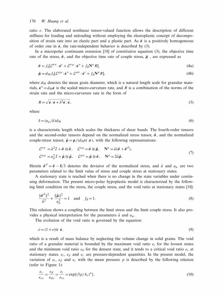
Granular materials show strong pressure- and density-sensitive behavior. For an initially densespecimen under monotonic loading to a stationary state, the deviatoric stress will show a peakwith the specimen experiencing dilation after an initial contraction. The denser the specimenis packed, the higher the peak and the stronger the dilation will be. The peak will be lesspronounced at a higher pressure level. If a specimen is initially in a very loose state, no peakstate will be displayed and the specimen will experience a consistent contraction without dila-tion. This pressure and density effect has been taken into account in the present hypoplasticmodel by including the void ratio as a state variable. For monotonic loading paths, accessiblestress states are bounded by the peak stress states, which form a conical surface in the princi-pal stress space with its apex at the origin and its axis aligned with the hydro-static pressureaxis.

With regard to criteria (30) and (46), we note that shear bifurcation depends on the stressand density for a non-polar continuum and the stress, couple stress and density for a micro-polar continuum (the couple stress often equals zero in a homogeneously deforming speci-men). Shear bifurcation will occur in a homogeneously deforming specimen as the criterion(30) or (46) is met by the varying stress and density. For the non-polar continuum model, ithas been shown that shear bifurcation occurs before the peak stress state is reached in biax-ial compression tests [23,24]. The bifurcation point and the inclination of the shear band areinfluenced by the initial density and the mean pressure. Wu and Sikora [25] and Wu [26], intheir analysis for bifurcation and failure in a density-independent non-polar hypoplastic con-tinuum, have shown that the peak stress state may be reached before the bifurcation conditionis met for some loading paths. This means a homogeneously deforming specimen may expe-rience either a homogeneous failure or a localized failure, depending on the loading path.

In order to investigate the possibility of bifurcation in a general way for the present con-tinuum models, we will compare the bifurcation states with the peak stress states in the devi-atoric stress plane, as done by Wu [26] for a density-independent hypoplastic model. For thispurpose, a mathematical representation for the peak stress state is formulated in the following.

178 W. Huang et al.

5.1. Peak stress state

A peak stress state is defined by a vanishing stress rate with e > 0. Note that a peak statediffers from a stationary state in that the void ratio vanishes simultaneously with the latter.We consider loading programs such that the directions of the principal stresses do not changewhile the deviatoric stress varies. Triaxial compression and extension, as well as biaxial com-pression and extension tests, are examples of these loading programs. In these cases, macro-spin does not develop and the peak stress state corresponds to fs(L : ε−fdN||ε||)=0, whichyields

ε=fdL−1 : N, (50)

where ε= ε/‖ε‖ is the normalized strain rate. Since ||ε||= 1, the following condition for thepeak stresses is obtained:

�p(σ )= (L−1 : N) : (L−1 : N)=1/f 2d . (51)

Herein �b is a function of σ (or σd ) only. Note that this peak stress state representation is

also relevant to the micro-polar hypoplastic model if couple stress and micro-curvature rateare zero. Given the representations for L and N in (13), L−1 and �b(σ ) become

L−1= 1a2

I− σ ⊗ σ

a2(a2+||σ ||2) , (52)

�p(σ )= 1a2

[η2||σ ||2+ (2η+1)||σ d ||2] (53)

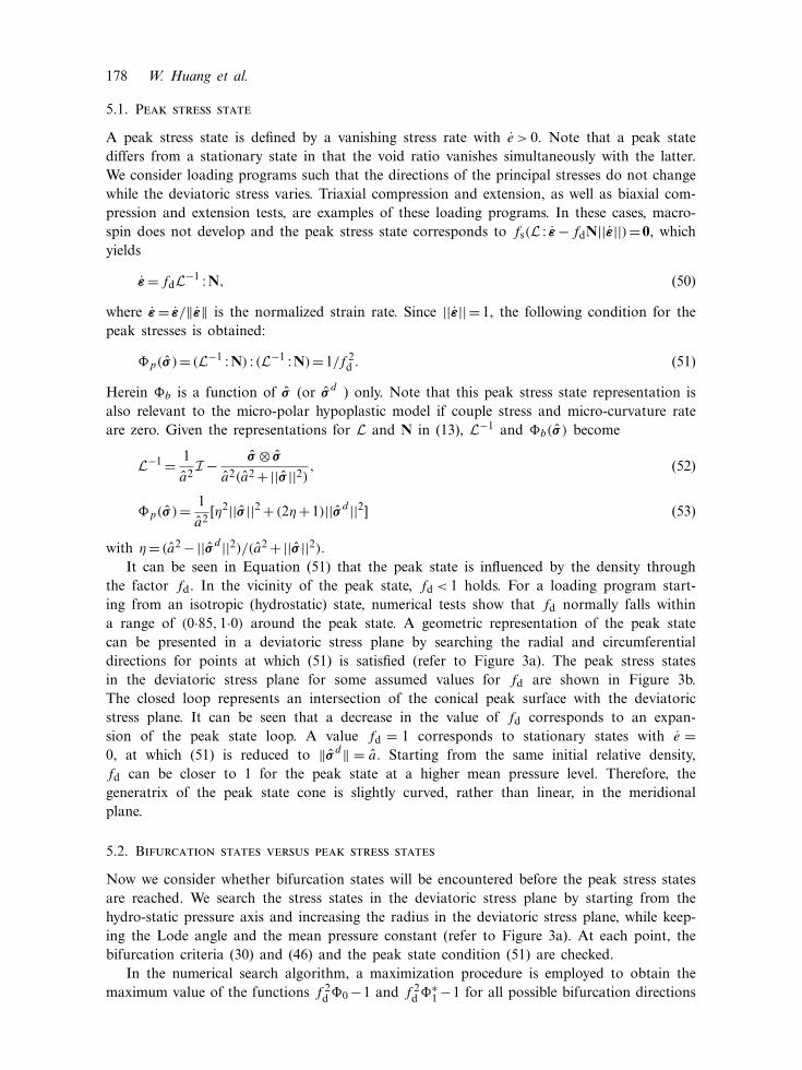
with η= (a2−||σ d ||2)/(a2+||σ ||2).It can be seen in Equation (51) that the peak state is influenced by the density through

the factor fd. In the vicinity of the peak state, fd < 1 holds. For a loading program start-ing from an isotropic (hydrostatic) state, numerical tests show that fd normally falls withina range of (0·85,1·0) around the peak state. A geometric representation of the peak statecan be presented in a deviatoric stress plane by searching the radial and circumferentialdirections for points at which (51) is satisfied (refer to Figure 3a). The peak stress statesin the deviatoric stress plane for some assumed values for fd are shown in Figure 3b.The closed loop represents an intersection of the conical peak surface with the deviatoricstress plane. It can be seen that a decrease in the value of fd corresponds to an expan-sion of the peak state loop. A value fd = 1 corresponds to stationary states with e =0, at which (51) is reduced to ‖σ d‖ = a. Starting from the same initial relative density,fd can be closer to 1 for the peak state at a higher mean pressure level. Therefore, thegeneratrix of the peak state cone is slightly curved, rather than linear, in the meridionalplane.

5.2. Bifurcation states versus peak stress states

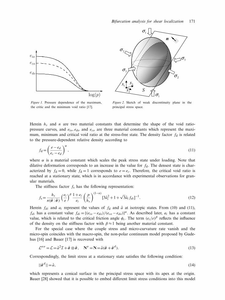
Now we consider whether bifurcation states will be encountered before the peak stress statesare reached. We search the stress states in the deviatoric stress plane by starting from thehydro-static pressure axis and increasing the radius in the deviatoric stress plane, while keep-ing the Lode angle and the mean pressure constant (refer to Figure 3a). At each point, thebifurcation criteria (30) and (46) and the peak state condition (51) are checked.

In the numerical search algorithm, a maximization procedure is employed to obtain themaximum value of the functions f 2

d�0−1 and f 2d�

∗1−1 for all possible bifurcation directions

Bifurcation analysis for shear localization 179

(a) (b)

Figure 3. Representation of peak stress on the deviatoric stress plane.

(a) (b)

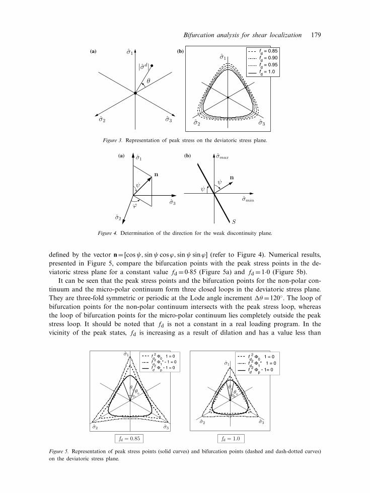
Figure 4. Determination of the direction for the weak discontinuity plane.

defined by the vector n= [cosψ, sinψ cosϕ, sinψ sinϕ] (refer to Figure 4). Numerical results,presented in Figure 5, compare the bifurcation points with the peak stress points in the de-viatoric stress plane for a constant value fd=0·85 (Figure 5a) and fd=1·0 (Figure 5b).

It can be seen that the peak stress points and the bifurcation points for the non-polar con-tinuum and the micro-polar continuum form three closed loops in the deviatoric stress plane.They are three-fold symmetric or periodic at the Lode angle increment θ=120◦. The loop ofbifurcation points for the non-polar continuum intersects with the peak stress loop, whereasthe loop of bifurcation points for the micro-polar continuum lies completely outside the peakstress loop. It should be noted that fd is not a constant in a real loading program. In thevicinity of the peak states, fd is increasing as a result of dilation and has a value less than

Figure 5. Representation of peak stress points (solid curves) and bifurcation points (dashed and dash-dotted curves)on the deviatoric stress plane.

180 W. Huang et al.

1·0. Since an increase in fd corresponds to a shrinking of the peak state and the bifurcationloops, the distance between the bifurcation points and the peak point in an arbitrary directionmay be smaller. However, in the specific directions where the bifurcation point coincides withthe peak point, fd must have a unique value at this point. Therefore, the relative positions ofthese loops are correctly shown in Figure 5.

Bearing in mind that only stress states inside the peak stress loop are accessible, we caninterpret these results as follows. In the non-polar continuum, shear bifurcation may occurbefore the peak state is reached for stress paths with a Lode angle θ ∈ [0, θ0) and θ ∈ (θ1,120◦].For stress paths with θ ∈ (θ0, θ1), which includes the stress path for a triaxial compression test,the peak state is reached before bifurcation. This indicates that a homogeneous loading willlead to a homogeneous failure or peak failure rather than a localized failure. A similar resultwas also obtained in [26] with an amorphous hypoplastic model (i.e., a hypoplastic modelwith the Cauchy stress being the only state variable).

In contrast to the possible shear bifurcation in the non-polar continuum, Figure 5 showsthat no bifurcation point will be reached before the peak state in the micro-polar continuum,even though the bifurcation states lie close to the peak states for a smaller Lode angle. Thisresult means that there is no solution for the discontinuity vector gu within the accessiblestress domain (which is an area in the principal stress space surrounded by a cone-shapedpeak-stress surface with its apex at the origin), which indicates that only homogeneous fail-ure or peak failure will occur in a homogeneously deforming continuum body. As no restric-tion has been put on vector gu, the result also rules out a co-axial solution of gu with respectto n. In other words, pure compression or tension localization is excluded too. In an earlieranalysis of localized failure with a micropolar elastoplastic model, Iordache and Willam [27]found that the micropolar continuum description suppresses localization bifurcation in shear.It may not suppress localization bifurcation in pure tension. This is, however, not in contra-diction with our results, since the micropolar hypoplastic model used in this study is definedonly in a compressive sub-domain in the principal stress space, as a cohesionless granularmaterial can not sustain tension. While localized failure is widely observed experimentally inbiaxial compression tests [31,32], peak failures have also been observed in triaxial compres-sion tests [33] and in true triaxial tests [34]. It should be pointed out that in the bifurcationanalysis, ideally homogeneous states are assumed in the continuum. However, in a real granu-lar medium some packing inhomogeneity is inevitable. On the micro-scale, the void ratio var-ies significantly from point to point even though a macroscopically homogeneous conditionis maintained. Shahinpoor [35] showed that even within a granular body composed of equal-sized spheres, the void ratio or porosity will not be uniform. This inhomogeneity of the voidratio can lead to a fluctuation in stress as well on the micro-scale when a granular specimenis loaded uniformly on its boundary. Numerical results have shown that such a state fluctu-ation is sufficient to initiate shear localization in a granular specimen undergoing a uniformloading process [36,37]. Therefore, in the micro-polar hypoplastic description, shear localiza-tion may occur, not in the form of sudden shear bifurcation, but rather in the form of con-tinuous development of deformation inhomogeneity as a result of state fluctuation and strainsoftening.

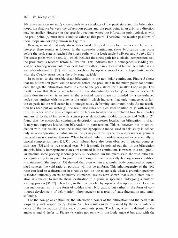
For the non-polar continuum, the intersection points of the bifurcation and the peak stateloops vary with respect to fd (Figure 5). This result can be explained by the density-depen-dence of the inclination of the weak discontinuity plane. The latter, which is defined by theangles ϕ and ψ (refer to Figure 4), varies not only with the Lode angle θ but also with the

Bifurcation analysis for shear localization 181

Figure 6. Inclination of the weak discontinuity plane in the non-polar hypoplastic continuum.

density factor fd. Numerical results for the non-polar continuum show that

ϕ={

180◦ for θ ∈ [0,60◦),90◦ for θ ∈ (60◦,120◦]

which means that the weak discontinuity plane has its normal perpendicular to the interme-diate principal stress direction. In other words, the weak discontinuity will occur in the planedefined by the maximum and minimum principal stresses. The inclination of the discontinu-ity plane is, however, influenced by the intermediate principal stress since ψ varies with thevariation of the Lode angle θ (Figure 6). An increase in the inclination of the discontinuityplane is obtained for a smaller value for fd. The intersection points between the bifurcationloop and the peak loop are marked in Figure 6. Between these marks a homogeneous failureis predicted.

6. Conclusion

Shear localization in granular materials has been studied at the constitutive model level as abifurcation problem. The materials have been modelled as a non-polar continuum and as amicro-polar continuum using a hypoplastic description. The bifurcation conditions have beenformulated in a general manner for the two incrementally nonlinear constitutive models. Theseconditions indicate that shear bifurcation depends on the stress and density state in the non-polar continuum and on the couple stress state as well in the micro-polar continuum. Thepossibility of shear localization has been examined using a geometric interpretation for thebifurcation states and the peak stress states in the principal stress space. The peak stress statesform a conical surface in the principal stress space bounding the accessible stress domain. Thestress states for bifurcation have been identified on the deviatoric stress plane and comparedwith the peak stress states. The results show that, in the non-polar hypoplastic continuum,weak discontinuity bifurcation will occur in certain loading paths, whereas in the micro-polarhypoplastic continuum, weak discontinuity bifurcation will never occur.

In the non-polar continuum description of material behaviour, occurrence of shear locali-zation is often attributed to the weak discontinuity bifurcation, a mathematical property asso-ciated with the constitutive models of this type. The bifurcation analyses for the micro-polarhypoplastic continuum in this work and for a micro-poplar elastoplastic continuum by Iord-ache and Willam suggest that the property of weak discontinuity bifurcation may no longer

182 W. Huang et al.

be associated with a micro-polar constitutive model. And shear localization at the constitutivemodel level may generally be suppressed in the micro-polar continuum description of materialbehaviour. While shear localization has been widely observed in experiments and engineer-ing practice, this physical phenomenon now can be interpreted as only a result of structureresponse. The inhomogeneity at the micro-structure level, the inevitably existing state fluctua-tion and the strain softening are the main causes leading to shear localization in a homoge-neous-on-the-macro-level granular body.

Acknowledgement

The financial support by Australia Research Council (grant DP0453056) is acknowledged bythe first author.

Appendix A

Let A be a partitioned square matrix in the form of

A=[

A11 A12

A21 A22

].

If A is invertible, its inverse

B=A−1=[

B11 B12

B21 B22

]can be obtained by

B22= (A22−A21 ·A−111 ·A12)

−1,

B12=−A−111 ·A12 ·B22,

B21=−B22 ·A21 ·A−111 ,

B11=A−111 −B12 ·A21 ·A−1

11 .

This representation shows that the invertibility of A depends on A11 and A22−A21 ·A−111 ·A12

being invertible. If A stands for � and we neglect the terms P′′uu and P′′wu for p<<fs, wehave

A11=P′uu,A12=Puw,A21=P′wu,A22=Pww.

Referring to expression (37), A11 and A22 are basically invertible. In particular,

A−111 =

1a2

(I− tn⊗ tn

a2+‖tn‖2

),

where tn = σ · n denotes the normalized traction on plane S. Furthermore, by inserting allcomponents in this expression, the following representation can be obtained:

A22−A21 ·A−111 ·A12=d50

[a2µI+

(1− 1

a2+‖tn‖2

)mn⊗ mn

],

where mn = µ · n denotes the normalized couple traction on plane S. Obviously A22 −A21 ·A−1

11 ·A12 is invertible, too.

Bifurcation analysis for shear localization 183

References

1. J.R. Rice, The localization of plastic deformation. In: W.T. Koiter (ed.), Theoretical and Applied Mechanics.North-Holland Publishing Company, Amsterdam (1976) pp. 207–220.

2. J.W. Rudnicki and J.R. Rice, Conditions for the localization of deformation in pressure-sensitive dilatantmaterials. J. Mech. Phy. Solids 23 (1975) 371–394.

3. I. Vardoulakis, Bifurcation analysis of the plane rectilinear deformation on dry sand sample. Int. J. SolidsStruct. 17 (1981) 1085–1101.

4. N.S. Ottosen and K. Runesson, Properties of discontinuous bifurcation solutions in elasto-plasticity. Int. J.Solids Struct. 27 (1976) 401–421.

5. J.P. Bardet and I. Vardoulakis, The asymmetry of stress in granular media. Int. J. Solids Struct. 38 (2001)353–367.

6. W. Ehlers, E. Ramm, S. Diebels and G.A. D’Addetta, From particle ensembles to Cosserat contiua: homog-enization of contact forces towords stress and couple stresses. Int. J. Solids Struct. 40 (2003) 6681–6702.

7. H.-B. Muhlhaus, Scherfugenanalyse bei granularem Material in Rahmen der Cosserat-Theorie. Ingenieur-Archiv 56 (1986) 389–399.

8. R. de Borst, Simulation of strain localization: a reappraisal of the Cosserat-continuum. Engng. Comp. 8(1991) 317–332.

9. A. Dietsche, P. Steinmann and K.J. Willam, Micropolar elasto-plasticity and its role in localization analysis.Int. J. Plast. 9 (1993) 813–831.

10. W. Ehlers and W. Volk, On theoretical and numerical methods in the theory of porous media based onpolar and non-polar solid materials. Int. J. Solids and Struct. 35 (1998) 4597–5616.

11. J. Tejchman, Modelling of shear localisation and autogeneous dynamic effects in granular bodies. Veroffent-lichungen des Institutes fur Bodenmechanik und Felsmechanik der Universitat Fridericiana in Karlsruhe, Heft140 (1997).

12. J. Tejchman and E. Bauer, Numerical simulation of shear band formation with a polar hypoplastic model.Comp. Geotech. 19 (1996) 221–244.

13. E. Bauer and W. Huang, Numerical study of polar effects in shear zones. In: Pande and Pietruszczakand Schweiger (eds.), Numerical Models in Geomechanics–NUMOG VII. Rotterdam: A.A. Balkema (1999)pp. 133–138.

14. J. Tejchman and G. Gudehus, Shearing of a narrow granular layer with polar quantities. Int. J. Numer.Anal. Meth. Geomech. 25 (2001) 1–28.

15. W. Huang and E. Bauer, Numerical investigations of shear localization in a micro-polar hypoplastic material.Int. J. Numer. Anal. Meth. Geomech. 5 (2003) 124–148.

16. G. Gudehus, A comprehensive constitutive equation for granular materials. Soils Found. 36 (1996) 1–12.17. E. Bauer, Calibration of a comprehensive hypoplastic model for granular materials. Soils Found. 36 (1996)

13–26.18. W. Huang, K. Nubel and E. Bauer, Polar extension of a hypoplastic model for granular materials with

shear localization. Mech. Mat. 34 (2002) 563–576.19. D. Kolymbas, Bifurcation analysis for sad samples with a non-linear constitutive equation. Ingenieur-Archiv

50 (1981) 131–140.20. R. Chambon and J. Desrues, Bifurcation par localisation et non linearite incrementale: un example heuris-

tique d’analyse complete. In: Plasticity Instability. Paris: Press ENPC. (1985) pp. 101–119.21. J. Desrues and R. Chambon, Shear band analysis for granular materials: The question of incremental non-

linearity. Ingenieur-Archiv 59 (1989) 187–196.22. R. Chambon, S. Crochepeyer and J. Desrues, Localization criteria for non-linear constitutive equations of

geomaterials. Mech. Cohesive-Fric. Mater. 5 (2000) 61–82.23. E. Bauer and W. Huang, The dependence of shear banding on pressure and density in hypoplasticity. In:

Adachi, Oka and Yashima (eds.), Localization and Bifurcation Theory for Soils and Rocks. Rotterdam: A.A.Balkema (1998) pp. 81–90.

24. E. Bauer, Analysis of shear band bifurcation with a hypoplastic model for a pressure and density sensitivegranular mateiral. Mech. Mater. 31 (1999) 597–609.

25. W. Wu and Z. Sikora, Localized bifurcation in hypoplasticity. Int. J. Engng. Sci. 29 (1991) 195–201.26. W. Wu, Non-linear analysis of shear band formation in sand. Int. J. Numer. Anal. Meth. Geomech. 24 (2000)

245–263.

184 W. Huang et al.

27. M.-M. Iordache and K. Willam, Localized failure analysis in elastoplastic Cosserat continua. Comput. Meth-ods Appl. Mech. Engng. 151 (1998) 559–586.

28. E. Bauer, Conditions for embedding Casagrande’s critical states into hypoplasticity. Mech. Cohesive-Frict.Mater. 5 (2000) 124–148.

29. I. Herle and G. Gudehus, Determination of parameters of a hypoplastic constitutive model from propertiesof grain assemblies.. Mech. Cohesive-Fric. Mater. 4 (1999) 461–486.

30. G.A. Holzapfel, Nonlinear Solid Mechanics–A Continuum Approach for Engineering. Chichester: John Wiley(2001) 455 pp.

31. I. Vardoulakis and B. Graf, Calibration on constitutive models for granular materials using data from biaxialexperiments. Geotechnique 35 (1985) 299–317.

32. D. Mokni and J. Desrues, Strain localization measurements in undrained plane-strain biaxial tests on HostunRF sand. Mech. Cohesive-Fric. Mater. 4 (1998) 419–441.

33. P.V. Lade, Localization effects in triaxial tests on sand. In: Proc. IUTAM Symposium on Deformation andFailure of Granular Materials, Delft (1982) pp. 461–471.

34. Q. Wang and P.V. Lade, Shear banding in true triaxial tests and its effect on failure in sand. ASCE J.Engng. Mech. 127 (2001) 754–761.

35. M. Shahinpoor, Statistical mechanical considerations on storing bulk solids. Bulk Solids Handling 1 (1981)31–36.

36. K. Nubel, Experimental and numerical investigation of shear localization in granular material. Veroffentlich-ungen des Institues fur Bodenmechanik und Felsmechanik der Universitat Fridericiana in Karlsruhe, Heft 159(2003) 159 pp.

37. K. Nubel and W. Huang, A study of localized deformation pattern in granular media. Compt. Meth. Appl.Mech. Engng. 193 (2004) 2719–2743.