~~~orrn~KiaR Procesiing & ~unugeme~~ Vol. 24, No. 5, pp. 567-576, 1988 a~S73/88 f3.W + .OO Printed in Great Britain. Copyright 0 1988 Pergamon Press plc

MATHEMATICAL RELATIONS BETWEEN IMPACT FACTORS AND AVERAGE NUMBER OF CITATIONS

L. EGGHE LUC, Universitaire Campus, B-3610, Diepenbeek, Belgium* and UIA, Universiteitsplein 1,

B-2610, Wilrijk, Belgium

(Received 28 September 1987; accepted in final form 29 January 1988)

Abstract-Instead of the two-year impact factor as used in the Jo~r~ffl Citation Reports, there is much in favor of using x-year impact factors (x > 0). These impact factors are studied as a function of x and compared with the average number of citations per paper to papers that appeared in the journal x years ago. It is shown that both are equal if and only if the derivative of the impact-factor function is zero. Based on this, a simple clas- sification of impact-factor curves versus mean citation curves is established and exam- ples are given. These results are also applied to recent practical data that were obtained by Rousseau.

1. INTRODUCTION

Let c(k) be the number of citations that a journal receives in a fixed year to articles pub- Iished k years before. Let p(k) be the number of articles in that same journal k years before. Let

c(k) cx(k) = -.

P(k)

The impact factor of a journal (in a given fixed year), as defined by Garfield [2] is given by

IF = c(I) + c(2) P(l) + P(2) ’

(2)

For example, in year 1987 (year 0)

IF = number of citations in 1987 to articles in the journal of years 1985 and 1986

number of articles in the journal of years 1985 and 1986

Here 1986 is year 1 and 1985 is year 2. However, as pointed out in [4] (see also [3]), in some research areas this value of IF

is not ideal in the sense that, instead of considering two years, another number of years might produce a higher impact factor. If the two-year impact factor of Garfieid is good for measuring the importance of life science journals, the same cannot be said for math- ematics journals. As pointed out in [4] (see also [3]), one obtains the highest impact fac- tor when taking a four-year period, that is, when calculating:

IFf4) = c(l) + c(2) 4 c(3) + c(4)

P(l) + PW + P(3) + P(4).

One generally can define (cf. [3], [4])

(3)

I thank Dr. R. Rousseau for stimulating discussions on this paper. *Permanent address.

567

568 L. EGGHE

k$ C(k)

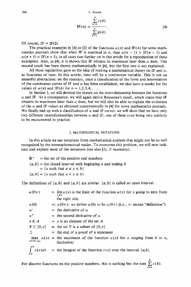
IF(n) = n . (4)

Of course, IF = IF(2). The practical examples in [4] or [3] of the functions cy(n) and IF(n) for some math-

ematics journals show that when IF is maximal in n, then cx (n - 1) > IF(n - 1) and a(n + 1) < IF(n + l), in all cases (see further on in this article for a reproduction of these examples). Also, in [4], it is shown that IF obtains its maximum later than cx does. This second result has been shown mathematically in [4], but the first one is not explained.

All these regularities gave us the idea of making a mathematical theory on IF and CY, as functions of time. In this article, time will be a continuous variable. This is not an unuseful abstraction; on the contrary, once a classification of the form and interrelation of the continuous curves of IF and 01 has been established, we also have a model for the values of a(n) and IF(n) for n = 1,2,3,4,. . . .

In Section 3, we will develop the theory on the interrelationship between the functions cy and IF. As a consequence, we will again derive Rousseau’s result, which states that IF obtains its m~imum later than CY does, but we will also be able to explain the evolution of the CY and IF values as obtained experimentally in [4] for some mathematics journals. We finally end up with a classification of (Y and IF curves: we will show that we have only two different interrelationships between 01 and IF, one of them even being very unlikely to be encountered in practice.

2. ~ATH~~AT~CAL NOTATIONS

In this article we use notations from mathematical analysis that might not be so well recognized by the nonmathematical reader. To overcome this problem, we will now indi- cate and explain most of the notations (see also [l], if necessary).

IR+ = the set of the positive real numbers

[a, b] = the closed interval with beginning (f and ending b = (xsuchthatasxrb)

]a,b] = (x such that a <XI b]

The definitions of [a, b [ and ] a, b [ are similar. 1 a, b [ is cahed an open interval.

cu(o+) = !~a (x) is the limit of the function a(x) for x going to zero from 9

the right side.

o (0) =: CY (O-t ) : we define cx (0) to be Q (0+ ) (i.e., =: means “definition”)

CX’ = the derivative of a!

CYs = the second derivative of (Y

XEA = x is an element of the set A

vc lO,x[ = the set V is a subset of ] O,x[

cl = the end of a proof of a statement

max (Y(X) = the maximum of the function cu(x) for x ranging from 0 to x0 XE lO,XOl (inclusive)

s

b

c(x)dx = the integral of the function c(x) over the interval [a$]. a

For discrete functions on the positive numbers, this is nothing but the sum i c(k). k=a

Impact factors and citations

3. THEORY OF THE FUNCTIONS a AND IF AND

EXPLANATIONS OF EXPERIMENTAL RESULTS

569

3.1 Definitions Let us fix a year (to be considered as the present year from which we will study the

past) and a journal. Let x > 0. Denote by c(x) the distribution function of the citations in this year to articles in this journal that were published x years ago. Analogously, let p(x) denote the distribution function of the articleszin this journal, x years ago.

Remark I. Of course, only J’ c(x)dx, 1 c(x)dx and so on are known in practice

(the same for the function p). Nevertheless, s&e time is continuous, we can interpret c(x) and p(x) for continuous time x > 0. We will see that our theory will yield new results for continuous x > 0. Then taking x = 1,2,3, . . . , we will see that our theory is able to pre- dict regularities that are encountered in practical examples.

c(x) Let (Y(X) = -, for x > 0. P(X)

We assume the following, very weak and natural, properties of the functions (Y and p.

(11= [O,M] - IR’

(with M very high; in practice, this is the number of years ago that the journal was founded).

o(O) = a(O+) = tmOa(x). 9

(Y is continuously differentiable and CY’ (x) > 0 for every x E [0,6], for a certain 6 > 0. We also suppose that there exists an x E ]O,M[, such that (Y’(X) = 0 and (Y”(X) < 0.

Remark 2. Note that the second-to-last property of the function cx does not follow from the other ones; to see this, just consider the function cry(x) = x + x sin l/x.

Remark 3. The fact that we require CX’ to be strictly positive, at least in a small interval starting in zero, is very natural and is always encountered in practice. Indeed, requiring (Y’ > 0 in a small interval starting in zero is equivalent with saying that CY is strictly increas- ing in the beginning. This is natural, except for those articles that are never cited (a! is con- stantly zero then), every article starts influencing others for a small or longer period in time. Gradually, the article is used more and more in this time period. In the life sciences, this time period is approximately two years; for mathematics this period is approximately four years. How long this period is is of no importance here; the existence of it suffices in our arguments. That is why we suppose the existence of a 6 > 0 (possibly small) such that (Y’ > 0 on [0,6].

Remark 4. Requiring that CY’ (x) = 0 and CY” (x) < 0 for a certain x E ]O,M[ is also very logical: the older the volumes of a journal are, the less they are used, at least after a certain time; it is never true that the older a journal volume is, the more it is used; this can be so in the beginning years but certainly not forever; Q’(X) = 0 and CX” (x) < 0 for a certain x > 0 expresses this fact.

About the function p we just assume

p= [O,M]+IR+

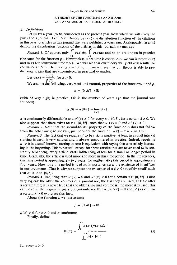
p(x) > 0 for x > 0 and p continuous. Finally, define

s x

CY (x’)p(x’)dx’

’ IF(x) =

s

x

p(x’)dx’ 0

(5)

for every x > 0.

570

3.2 Basic theory of CI and IF

L.EGGHE

All results taken from infinitesimal analysis can be found, for instance, in [l].

PROPOSITION 1 IF(O+) = CY (O+ ) . Proof. Using de 1’Hospital’s rule, we see that

IF(O+) = F$IF(x) = lim a (X)P(X) = a(O+).

> X20 P(X)

THEOREM 1

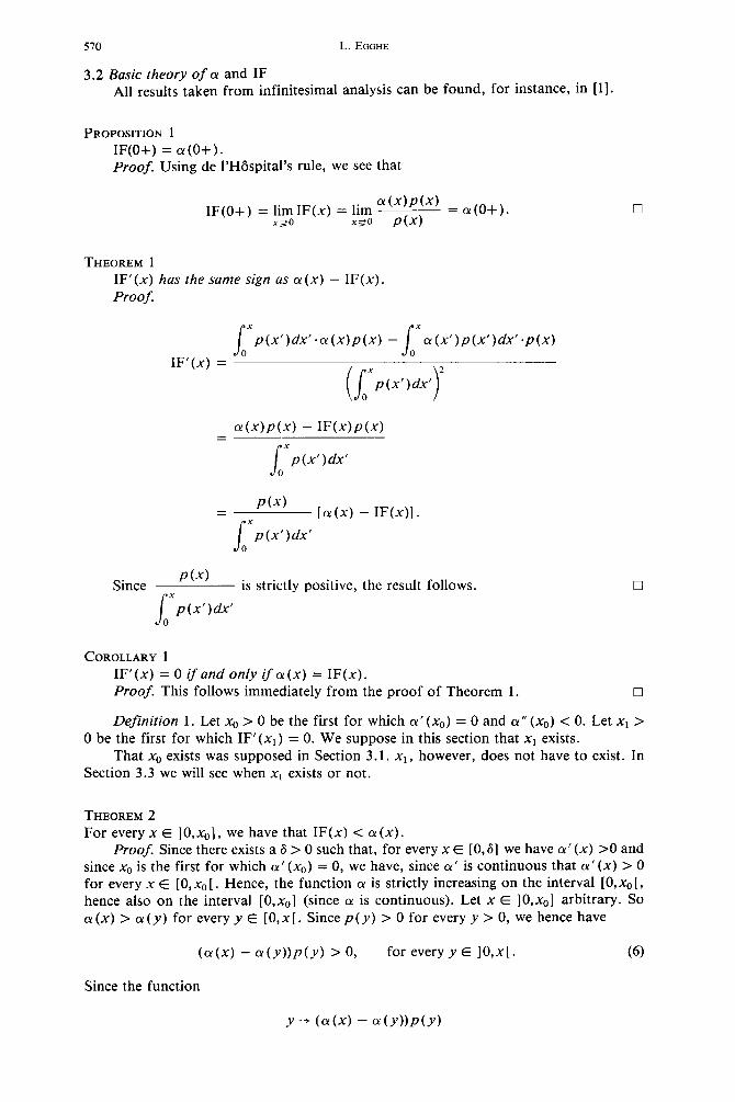
IF’(x) has the same sign as a(x) - IF(x). Proof.

s x

p(x’)dx’*a(x)p(x) - a(x’)p(x’)dx’*p(x)

’ IF’(x) = 2

Q(X)P(X) - IF(x)p(x)

J p(x’)dx’ 0

P(X) = [a(x) - IF(x)I.

s

x p(x’)dx’

0

Since P(X)

is strictly positive, the result follows.

s

X p(x’)dx’

0

q

COROLLARY 1

IF’(x) = 0 ifand only ifa = IF(x). Proof. This follows immediately from the proof of Theorem 1. 0

Definition 1. Let x0 > 0 be the first for which CY’ (x0) = 0 and CY” (x0) c 0. Let x1 > 0 be the first for which-IF/(x,) = 0. We suppose in this-section that x1

That x0 exists was supposed in Section 3.1. x1, however, does not Section 3.3 we will see when x, exists or not.

exists. have to exist. In

THEOREM 2

For every x E 10,x0], we have that IF(x) < a(x). Proof. Since there exists a 6 > 0 such that, for every x E [0,6] we have a’(x) >O and

since x0 is the first for which CY’ (x0) = 0, we have, since CY’ is continuous that (Y’(X) > 0 for every x E [O,xo[. Hence, the function (Y is strictly increasing on the interval [0,x01, hence also on the interval [0,x0] (since CY is continuous). Let x E ]O,xo] arbitrary. So a(x) > a(y) for every y E [O,x[. Sincep(y) > 0 for every y > 0, we hence have

(a(x) - cy(Y))P(Y) > 0, for every y E ]O,x[. (6)

Since the function

Y -+ (al(x) - Q(Y))P(Y)

Impact factors and citations 571

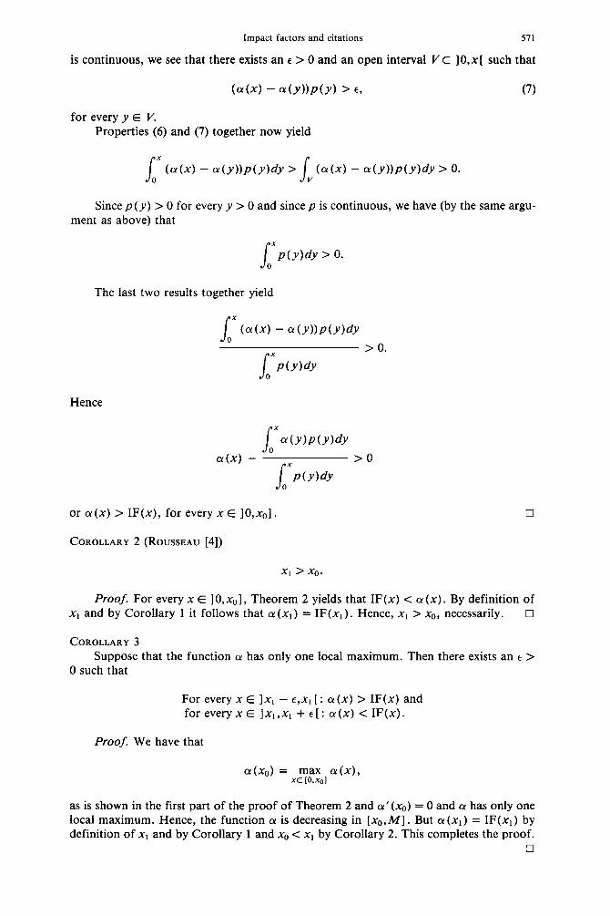
is continuous, we see that there exists an E > 0 and an open interval V C ]O,x[ such that

(a(x) - U(Y))P(Y) > f9 (7)

for every y E V. Properties (6) and (7) together now yield

s x (a(x) - cr(Y))P(Y)dY > s (a(x) - a(Y))P(Y)dY > 0. 0 V

Since p (y) > 0 for every y > 0 and since p is continuous, we have (by the same argu- ment as above) that

s oxP(Y)dY > 0.

The last two results together yield

s x

(a(x) - c-r(Y))P(Y)dY 0

> 0.

s

x

p(y)& 0

Hence

s x

a (y)p(y)& 0

a(x) - >o

S x

p(y)& 0

or CY(X) > IF(x), for every x E ]O,xo].

COROLLARY 2 (ROUSSEAU [4])

XI > x0.

Proof. For every x E ] 0,x0], Theorem 2 yields that IF(x) < Q (x) . By definition of x1 and by Corollary 1 it follows that CY(X,) = IF(x,). Hence, xl > x0, necessarily. 0

COROLLARY 3

Suppose that the function (Y has only one local maximum. Then there exists an E > 0 such that

For every x E lx, - 6,x1 [: a(x) > IF(x) and for every x E 1x1,x1 + E[: a(x) < IF(x).

Proof. We have that

a(xo) = xEyoyol a(x),

as is shown in the first part of the proof of Theorem 2 and c-w’(xo) = 0 and Q has only one local maximum. Hence, the function (Y is decreasing in [xo,M] . But CY (xi) = IF(x, ) by definition of x1 and by Corollary 1 and x0 < x1 by Corollary 2. This completes the proof.

cl

572 L. EGGHE

COROLLARY 4 For every x E ] 0, x1 1, IF'(x) > 0 and hence IF is strictly increasing on [0,x1 ] . Proof. From Theorems 1 and 2 we have already that IF is strictly increasing on the

interval ]O,x,,] . Suppose now that IF does not increase strictly on ]xo,xl] . So, there is a y E ]x,,,x, [ and an E > 0, such that IF’(x) I 0 for every x E ]y - e,y + E [ (since IF is continuous). Since IF’(x) > 0 for every x E 10,x0], we must have that IF’(y) = 0 for a certain y. E ]xo,y] c 10,x1 [ (hence, y < x1).

But x1 was supposed to be first for which IF/(x,) = 0, a contradiction. Hence, IF is strictly increasing on the interval 10,x1]. From this, of course, it follows that IF’(x) > 0, for everyxE 10,x1]. I?

COROLLARY 5

For every x E 10,x, [

IF(x) < a(x).

Proof. This follows immediately from Theorem 1 and Corollary 4. 0

Remark 5. By the special form of eqn (5), we can also apply the weighted mean value theorem for integrals (since 01 2 0 and continuous in [0, M] and p > 0 and continuous in ]O,M]) (cf. [l], p. 325). Hence we find for every x E ]O,M], there is a point c, E [0,x] such that

CY(C,) = IF(x).

From this, we can conclude that IF(x) takes the CY values in a “retarded” way (since c, 5 x).

3.3 Classification of the possible relations between (Y and IF In all cases, both CY and IF start (in 0) at the same point, by Proposition 1. If the value

in 0 is not 0, this shows the existence of invisible colleges, which can indeed be the case. Only invisible colleges are responsible for (Y (0) > 0: fast, direct communication of research results through preprints or oral communication; journals are not likely to react upon each other with this speed (except in special circumstances where the publication date of a jour- nal differs substantially from the date that is printed on it).

In all cases, IX starts increasing (by assumption), and hence, since IF is a weighted aver- age of a values, the same is true with IF. Because it is an average, IF(x) < Q(X) in a cer- tain interval [O,y] , y > 0.

In Section 3.1 we showed that it was natural to suppose that there is an x > 0 such that IX’(X) = 0 and a”(x) < 0. So, by Definition 1, x0 exists. Thus, in any case, the func- tion cx has its first local maximum in x0.

Now, after x0, we can have that the function CY keeps on decreasing, or it starts increasing in a certain pointy > x0. Suppose first that cx keeps on decreasing. In this case xi, being the intersection of CY and IF (by Corollary 1 and Definition 1) always exists. Indeed, so far IF was increasing; it can only start decreasing after a point where IF’ is zero. But then, by Corollary 1, the curves (Y and IF intersect necessarily. In Definition 1, x1 was called the first such point.

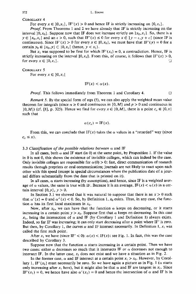
After x1 we have (since IF’ < 0): a(x) < IF(x): see Fig. 1. In fact, this was the case described by Corollary 3.

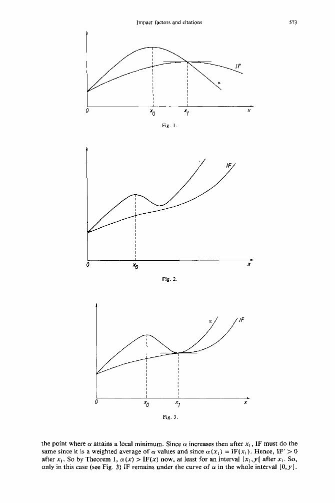
Suppose now that the function u starts increasing in a certain point. Then we have two cases: either CY decreases so much that it intersects IF or a! decreases not enough to intersect IF. In the latter case, x1 does not exist and we have a situation as in Fig. 2.

In the former case, (Y and IF intersect at a certain point x1 > x0. However, by Corol- lary 1, IF/(x,) must necessarily be zero. So we have again a picture as in Fig. 1 (a starts only increasing after x1 here), but it might also be that (Y and IF are tangent in xi. Since IF’(x,) = 0, we hence have also CX’ (xl) = 0 and hence the intersection of a! and IF is in

Impact factors and citations 573

Fig. 1.

I I I I

0 ‘b X

Fig. 2.

I I

I

I I

I I

I I

I I I

0 xO xl X

Fig. 3.

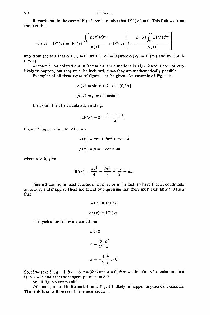
the point where cx attains a local minimum. Since (Y increases then after x1, IF must do the same since it is a weighted average of Q values and since CY (x1 ) = IF (xl ) . Hence, IF’ > 0 after x,. So by Theorem 1, (11 (x) > IF(x) now, at least for an interval [x1 ,y [ after x1. So, only in this case (see Fig. 3) IF remains under the curve of cx in the whole interval [O,y [.

514 L. EGGHE

Remark that in the case of Fig. 3, we have also that IF” (xi) = 0. This follows from the fact that

s

x

[

s

x p(x’)dx’ PI (xl p(x’)dx’

a’(x) - IF’(x) = IF”(x) ’ 0

P(X) + IF’(x) 1 -

P(XV 1 and from the fact that o’(xi) = 0 and IF/(x,) = 0 (since CY(X~) = IF(x,) and by Corol- lary 1).

Remark 6. As pointed out in Remark 4, the situations in Figs. 2 and 3 are not very likely to happen, but they must be included, since they are mathematically possible.

Examples of all three types of figures can be given. An example of Fig. 1 is

a(x) = sin x + 2, x E [0,3a]

p(x) = p = a constant

IF(x) can then be calculated, yielding,

IF(x) = 2 + 1 - cos x

x .

Figure 2 happens in a lot of cases:

01(x) =ax3+by2+cx+d

p(x) = p = a constant

where a > 0, gives

IF(x) = $ + 4 + y + c/x.

Figure 2 applies in most choices of a, b, c, or d. In fact, to have Fig. 3, conditions on a, b, c, and d apply. These are found by expressing that there must exist an x > 0 such that

a(x) = IF(x)

a’(x) = IF’(x).

This yields the following conditions

a>0

8 b2 C=ua

x=-4b>o Qa ’

So, if we take f.i. a = 1, b = -6, c = 32/3 and d = 0, then we find that (Y’S osculation point is in x = 2 and that the tangent point x1 = 8/3.

So all figures are possible. Of course, as said in Remark 5, only Fig. 1 is likely to happen in practical examples.

That this is so will be seen in the next section.

3 A Examples

Impact factors and citations 575

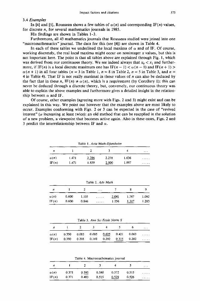
In [4] and [5], Rousseau shows a few tables of a(n) and corresponding IF(n) values, for discrete n, for several mathematics journals in 1985.

His findings are shown in Tables l-3. Furthermore, all 43 mathematics journals that Rousseau studied were joined into one

“macromathematics” journal. The data for this (see [4]) are shown in Table 4. In each of these tables we underlined the local maxima of CY and of IF. Of course,

working discretely, the real local maxima might occur on noninteger x values, but this is not important here. The point is that all tables above are explained through Fig. 1, which was derived from our continuous theory. We see indeed always that x0 < x1 and further- more, if IF(n) is a local discrete maximum one has IF( n - 1) < Q (n - 1) and IF( n + 1) > a! (n + 1) in all four tables (n = 3 in Table 1, n = 8 in Table 2, n = 5 in Table 3, and n = 4 in Table 4). That IF is not really maximal in those values of n can also be deduced by the fact that in these n, IF(n) # CY(FZ), which is a requirement (by Corollary 1): this can never be deduced through a discrete theory, but, conversely, our continuous theory was able to explain the above examples and furthermore gives a detailed insight in the relation- ship between CY and IF.

Of course, other examples (agreeing more with Figs. 2 and 3) might exist and can be explained in this way. We point out however that the examples above are most likely to occur. Examples conforming with Figs. 2 or 3 can be expected in the case of “revived interest” ((Y increasing at least twice): an old method that can be reapplied in the solution of a new problem, a viewpoint that becomes active again. Also in these cases, Figs. 2 and 3 predict the interrelationship between IF and CX.

Table 1. Acta Math-Djursholm

n 1 2 3 4

a(n) 1.471 2.286 2.278 1.636 . .._

IF(n) 1.471 1.839 2.ooo 1.887 . . . . .

Table 2. Adv Math

n 1 2 . 7 8 9

a(n) 0.600 1.105 . . 2.041 1.767 1.092 _

IF(n) 0.600 0.846 . 1.256 1.317 1.283

Table 3. Ann Sci Ecole Norm S

n 1 2 3 4 5 6

or(n) 0.350 0.083 0.095 0.625 0.421 0.063 . _

IF(n) 0.350 0.205 0.169 0.292 0.315 0.282 _

Table 4. Macromathematics journal

n 1 2 3 4 5

a(n) 0.371 0.595 0.580 0.572 0.515 . IF(n) 0.371 0.483 0.515 0.529 0.526 . _

516 L. EGGHE

REFERENCES

1. De Lillo, N.J. Advanced Calculus with Applications. London: Collier Macmillan Publ.; 1982. 2. Garfield; E. Citation analysis as a tool in journal evaluation. Science 178: 471-479; 1972. 3. Rousseau, R. Impact factors calculated over several periods with an application to mathematical journals. Pro-

ceedings 3rd National Conference with international participation on Scientometrics and Linguistics of the Scientific Text, Varna (Bulgaria), 14-16 May 1987. To appear.

4. Rousseau, R. Citation distribution of pure mathematics journals. Proceedings 1st International Conference on Bibliometrics and Theoretical Aspects of Information Retrieval (L. Egghe and R. Rousseau, eds.) LUC, Diepenbeek, 24-28 August 1987, pp. 249-262, 1988.