Embed Size (px)
Citation preview
Per Edström
DEPARTMENT OF ENgiNEERiNg, Physics AND MAThEMATics
Mid sweden University Doctoral Thesis 22
10 år
Mathematical Modeling and Numerical Tools for simulation and Design
of Light scattering in Paper and Print

Thesis for the degree of Doctor of PhilosophyHärnösand 2007
MATHEMATICAL MODELING AND NUMERICAL TOOLS FOR SIMULATION AND DESIGN
OF LIGHT SCATTERING IN PAPER AND PRINT
Per Edström
Supervisors:Professor Mårten Gulliksson, Mid Sweden University
Associate Professor Inge Söderkvist, Luleå University of Technology
FSCN Fibre Science and Communication NetworkDepartment of Engineering, Physics and MathematicsMid Sweden University, SE 871 88 Härnösand, Sweden
ISSN 1652 893X,Mid Sweden University Doctoral Thesis 22
ISBN 978 91 85317 50 9
FSCNFibre Science and Communication Network
- ett skogsindustriellt forskningsprogram vid Mittuniversitetet
ii
Akademisk avhandling som med tillstånd av Mittuniversitetet framläggs tilloffentlig granskning för avläggande av filosofie doktorsexamen tisdagen den 29maj 2007 klockan 13.00 i sal Sigma, Mittuniversitetet, Härnösand.Disputationen kommer att hållas på svenska.
MATHEMATICAL MODELING AND NUMERICAL TOOLS FOR SIMULATION AND DESIGN OF LIGHT SCATTERING IN PAPER AND PRINT Per Edström
© Per Edström, 2007
FSCN Fibre Science and Communication NetworkDepartment of Engineering, Physics and MathematicsMid Sweden University, SE 871 88 HärnösandSweden
Telephone: +46 (0)771 975 000
Printed by Hemströms Offset & Boktryck, Härnösand, Sweden, 2007
iii
MATHEMATICAL MODELING AND NUMERICAL TOOLS FOR SIMULATION AND DESIGN OF LIGHT SCATTERING IN PAPER AND PRINT Per Edström
FSCN Fibre Science and Communication NetworkDepartment of Engineering, Physics and MathematicsMid Sweden University, SE 871 88 Härnösand, SwedenISSN 1652 893X, Mid Sweden University Doctoral Thesis 22ISBN 978 91 85317 50 9
ABSTRACT
This work starts with a real industrial problem – the perceived need for a moredetailed and more accurate model for light scattering in paper and print than theKubelka Munk model of today. A careful analysis transfers this problem into aphysical description of the phenomena involved. This is then given a mathematicalformulation, and a detailed analysis leads to numerical solution procedures forspecific sub problems. Methods from scientific computing make it possible to meetindustrial demands made on speed and stability, and implementation in computercode is then followed by analysis of accuracy and stability.
A problem formulation and a solution method are outlined for the forwardradiative transfer problem. First, all necessary steps to arrive at a numericallystable solution procedure are treated, and then methods are introduced to increasethe speed by a factor of several thousands or millions compared to a naiveapproach. The method is shown to be unconditionally stable, though the problemwas previously considered numerically intractable, and systematic studies ofnumerical performance are presented.
The inverse radiative transfer problem is given a least squares formulation, anddifferent solution methods are analyzed and compared. Specifically, a two phasemethod for estimation of the scattering and absorption coefficients and theasymmetry factor ( s, a and g) is presented. A sensitivity analysis is given, and it isshown how it can be used for designing measurements with minimal impact frommeasurement noise.
It is shown how the standardized use of Kubelka Munk and the d/0°instrument leads to errors, and that the errors arising from an over idealized view
iv
of the instrument – due to the fact that instrument readings are incorrectlyinterpreted – can be larger than any errors inherent in the Kubelka Munk modelitself. It is argued that the measurement device and the simulation model cannot beviewed as separate instances, which is a widespread implicit practice in appliedreflectance measurements. Rather, given a measurement device, measurement datashould be interpreted through a model that takes into consideration the actualgeometry, function and calibration of the instrument.
The resulting tool, DORT2002, is in all aspects the Next Generation KubelkaMunk, and provides a greater range of applicability, higher accuracy and increasedunderstanding. It offers better interpretation of measurement data, and facilitatesthe exchange of data between the paper and graphical arts industries. It opens forunderstanding of anisotropic reflectance and for the utilization of the asymmetryfactor to design anisotropy, and thereby for the design of different visualappearance or optical performance in new printed or paper products.
Keywords: mathematical modeling; radiative transfer; integro differentialequations; inverse problems; parameter estimation; solution method; numericalperformance; light scattering; paper industry applications; Kubelka Munk
v
SAMMANDRAG
Detta arbete startar i ett konkret industriellt problem – behovet av en merdetaljerad och noggrann modell för ljusspridning i papper och tryck än dagensKubelka Munk modell. En omsorgsfull analys överför detta problem till enfysikalisk beskrivning av ingående fenomen. Denna ges sedan en matematiskformulering, och en detaljerad analys leder till numeriska lösningsprocedurer förspecifika delproblem. Beräkningsvetenskapliga metoder gör det möjligt att mötaindustriella krav på snabbhet och stabilitet, och implementation i datorkod följssedan av analys av noggrannhet och stabilitet.
En problemformulering och en lösningsmetod för det direkta radiative transferproblemet presenteras. Först behandlas alla steg som krävs för att få en numerisktstabil lösningsmetod, och sedan introduceras metoder för att ökaberäkningshastigheten med en faktor på flera tusen eller miljoner jämfört med ettnaivt tillvägagångssätt. Det visas att metoden är ovillkorligt stabil, trots attproblemet tidigare betraktats som numeriskt ohanterligt, och systematiska studierav numeriska prestanda redovisas.
Det inversa radiative transfer problemet ges en minsta kvadratformulering, ocholika lösningsmetoder analyseras och jämförs. Speciellt presenteras en tvåfasmetod för estimering av spridnings och absorptionskoefficienterna ochasymmetrifaktorn ( s, a och g). En känslighetsanalys ges, och det visas hur denkan användas för att utforma mätningar med minsta möjliga påverkan frånmätbrus.
Det visas hur användning av Kubelka Munk och d/0° instrument enligtstandarder leder till fel, och att felen som uppkommer från en alltför idealiseradsyn på instrumentet – till följd av att mätvärdena tolkas felaktigt – kan vara störreän de inneboende felen i Kubelka Munk modellen själv. Det påpekas attmätinstrument och simuleringsmodell inte kan ses som separata enheter, vilket ärimplicit gängse praxis vid tillämpade reflektansmätningar. I stället bör mätdata,givet ett mätinstrument, tolkas genom en modell som tar hänsyn till instrumentetsverkliga geometri, funktionssätt och kalibrering.
Det resulterande verktyget, DORT2002, är i alla avseenden Nästa GenerationsKubelka Munk, och tillhandahåller större tillämpningsområde, bättre noggrannhetoch ökad förståelse. Det erbjuder bättre tolkning av mätdata, och underlättarutbyte av data mellan pappersindustrin och den grafiska industrin. Det öppnar förförståelse av anisotrop reflektans och för användandet av asymmetrifaktorn fördesign av anisotropi, vilket möjliggör design av olika visuella intryck eller optiskrespons för nya tryckta pappersprodukter.
vi
Front cover illustration
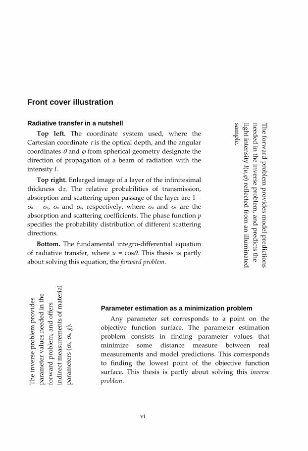
Radiative transfer in a nutshell Top left. The coordinate system used, where the
Cartesian coordinate is the optical depth, and the angularcoordinates and from spherical geometry designate thedirection of propagation of a beam of radiation with theintensity I.Top right. Enlarged image of a layer of the infinitesimal
thickness d . The relative probabilities of transmission,absorption and scattering upon passage of the layer are 1a s, a and s, respectively, where a and s are the
absorption and scattering coefficients. The phase function pspecifies the probability distribution of different scatteringdirections.Bottom. The fundamental integro differential equation
of radiative transfer, where u = cos . This thesis is partlyabout solving this equation, the forward problem.
Theforw
ardproblem
providesmodelpredictions
neededin
theinverse
problem,and
predictsthe
lightintensityI(u,
)reflectedfrom
anillum
inatedsam
ple.
Theinverseprob
lem
prov
ides
parameter
values
need
edin
the
forw
ardprob
lem,and
offers
indirectmeasurementsof
material
parameters(
s,a,g).
Parameter estimation as a minimization problem Any parameter set corresponds to a point on the
objective function surface. The parameter estimationproblem consists in finding parameter values thatminimize some distance measure between realmeasurements and model predictions. This correspondsto finding the lowest point of the objective functionsurface. This thesis is partly about solving this inverseproblem.
vii
Back cover illustration
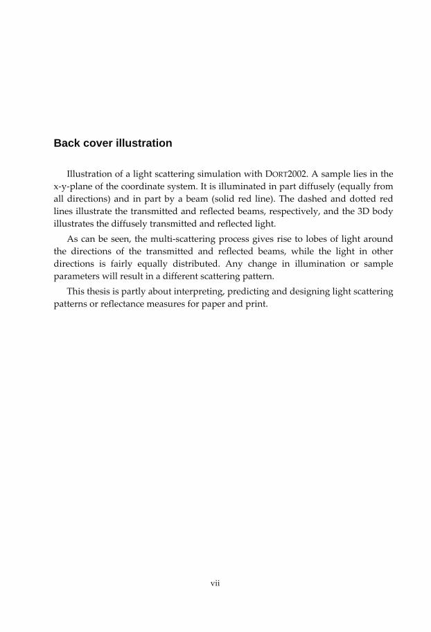
Illustration of a light scattering simulation with DORT2002. A sample lies in thex y plane of the coordinate system. It is illuminated in part diffusely (equally fromall directions) and in part by a beam (solid red line). The dashed and dotted redlines illustrate the transmitted and reflected beams, respectively, and the 3D bodyillustrates the diffusely transmitted and reflected light.
As can be seen, the multi scattering process gives rise to lobes of light aroundthe directions of the transmitted and reflected beams, while the light in otherdirections is fairly equally distributed. Any change in illumination or sampleparameters will result in a different scattering pattern.
This thesis is partly about interpreting, predicting and designing light scatteringpatterns or reflectance measures for paper and print.
viii
TABLE OF CONTENTS
ABSTRACT ...................................................................................................................... III
SAMMANDRAG............................................................................................................. V
LIST OF PAPERS ............................................................................................................ IX
0. IN RETROSPECT ......................................................................................................1
1. INTRODUCTION .....................................................................................................2
2. FROM INDUSTRIAL PROBLEM TO INDUSTRIAL TOOL............................22.1. STARTING WITH A REAL INDUSTRIAL PROBLEM.......................................................22.2. THE RADIATIVE TRANSFER PROBLEM ......................................................................3
2.2.1. A forward problem formulation......................................................................42.2.2. An inverse problem formulation.....................................................................4
2.3. SOLVING A REAL INDUSTRIAL PROBLEM .................................................................52.4. THE RESULTING SOFTWARE TOOL ...........................................................................5
3. MATHEMATICAL ANDNUMERICAL ESSENTIALS.....................................63.1. MORE ON THE FORWARD PROBLEM FORMULATION .................................................63.2. SOME DETAILS ON THE FORWARD SOLUTION METHOD ............................................7
3.2.1. Fourier analysis .............................................................................................73.2.2. Discretization .................................................................................................93.2.3. Preconditioning............................................................................................11
3.3. MORE ON THE INVERSE PROBLEM FORMULATION..................................................123.4. SOME DETAILS ON THE INVERSE SOLUTION METHOD.............................................13
4. A SHORT TOUR THROUGH THE PAPERS.....................................................14
5. A PATH TO PROBLEM INSIGHT.......................................................................165.1. WHAT IS ‘CORRECT’ IS RELATIVE TO THE ASSUMPTIONS MADE.............................18
6. ANISOTROPIC REFLECTANCE .........................................................................19
7. THE HIDDEN COMPLEXITY OF THEWORK.................................................21
8. DISCUSSION...........................................................................................................24
9. FUTUREWORK.......................................................................................................26
10. ACKNOWLEDGEMENTS.....................................................................................28
REFERENCES ...................................................................................................................30
ix
LIST OF PAPERS
This thesis is based on the following seven papers, herein referred to by theirrespective Roman numerals.
Paper I A Fast and Stable Solution Method for the Radiative TransferProblemPer EdströmSIAM Review, vol. 47, pp. 447 468 (2005)
Paper II Numerical Performance of Stability Enhancing and SpeedIncreasing Steps in Radiative Transfer Solution MethodsPer EdströmSubmitted to the Journal of Computational and AppliedMathematics (2007)
Paper III Comparison of the DORT2002 Radiative Transfer SolutionMethod and the Kubelka Munk ModelPer EdströmNordic Pulp and Paper Research Journal, vol. 19, pp. 397 403 (2004)
Paper IV Quantification of the Intrinsic Error of the Kubelka Munk ModelCaused by Strong Light AbsorptionHjalmar Granberg and Per EdströmJournal of Pulp and Paper Science, vol. 29, pp. 386 390 (2003)
Paper V Levenberg Marquardt Methods for Parameter EstimationProblems in the Radiative Transfer EquationTao Feng, Per Edström and Mårten GullikssonInverse Problems, vol. 23, pp. 879 891 (2007)
Paper VI A Two Phase Parameter Estimation Method for Radiative TransferProblems in Paper Industry ApplicationsPer EdströmSubmitted to Inverse Problems in Science and Engineering (2007)
Paper VII Examination of the Revised Kubelka Munk Theory:Considerations of Modeling StrategiesPer EdströmJournal of the Optical Society of America A, vol. 24, pp. 548 556(2007)
x
Publications not included in the thesis
P. Edström, Efficient Reflectance Calculations and Parameter EstimationMethods for Radiative Transfer Problems in Paper Industry Applications,Mid Sweden University, 2007.
C. Engström, N. Pauler, J. Wågberg and P. Edström, Final Report on theProject: Optical Interaction between Ink and Paper, Mid Sweden University,2007.
P. Edström and M. Lehto, Fast and Stable Solution Method for AngleResolved Light Scattering Simulation III – Handling Refractive IndexDiscontinuities, Mid Sweden University, 2005.
P. Edström,Mathematical Modelling of Light Scattering in Paper andPrint, Licentiate thesis, Mid Sweden University, 2004.
P. Edström and M. Lehto, Performance and Application of the DORT2002Light Scattering Simulation Model, Mid Sweden University, 2003.
P. Edström, A Comparison Between the Coefficients of the Kubelka Munkand DORT2002 Models, Mid Sweden University, 2003.
P. Edström and M. Lehto,DORT2002 version 2.0 User Manual, Mid SwedenUniversity, 2003.
P. Edström and M. Lehto, Fast and Stable Solution Method for AngleResolved Light Scattering Simulation II – Model Enhancements, MidSweden University, 2003.
P. Edström, Fast and Stable Solution Method for Angle Resolved LightScattering Simulation, Mid Sweden University, 2002.
P. Edström, H. Granberg and M. Gulliksson, Some Ideas on Models andMethods for Light Scattering in Paper, Mid Sweden University, 2001.
1
0. IN RETROSPECT
I was approached by the newly installed professor in System Analysis andMathematical Modeling, Mårten Gulliksson, and I was presented with two veryrespectable piles of paper: “I want you to be my PhD student, and I want you tochoose to work on either light scattering problems or diffusion problems”. I wentthrough both piles, and chose light scattering problems for no particular reason.
Nils Pauler of MoDo Paper R&D (now M Real) presented a poster at aninformation event at Mid Sweden University. The poster was about colorreproduction in digital printing. We had a short discussion, of which I nowremember nothing. However, I still remember the occasion, since for some reasonit was the start of a mutually rewarding paper optics journey that we still are on.
Very early in my work, I met with several companies in the paper industry. Wespoke of things I then knew very little about. Industrial relevance soon becameimportant to me. I find it beautiful when academic research provides results thatare relevant and available for industrial use.
I was called to the board of T2F (“TryckTeknisk Forskning”, a Swedish printingresearch program) to present my project. Since I had barely started the work, thepresentation was mainly based on intuition and self confidence. Somewhat laterT2F decided to support my PhD studies financially. This was also the ticket to awide network of future colleagues.
2
1. INTRODUCTION
The overall goals of the work presented in this thesis include the developmentof a fast and numerically stable solution procedure for the radiative transferproblem, and development, implementation and performance analysis ofalgorithms for the corresponding forward and inverse problems. The resultingsoftware tools should provide better accuracy and increased insight compared tothe Kubelka Munk model of today.
Applications should be made on relevant light scattering problems from thepaper and printing industries, and the final goal is the ability to solve a broadrange of problems within this area with sufficient speed and numerical stability.The method development ought to lead to algorithms that work well for appliedusers.
2. FROM INDUSTRIAL PROBLEM TO INDUSTRIAL TOOL
2.1. Starting with a real industrial problem Reflectance measurements are central for determining the optical properties of
paper and print, such as scattering and absorption parameters and opacity, butalso derived quantities like whiteness and color. This requires a light scatteringmodel, and the Kubelka Munk model [1 3] is prescribed by international standards[4 7] for such calculations in the paper industry. The model is easy to use, it isanalytically invertible, and although it is only a very coarse approximation, theaccuracy is often sufficient for industrial use. However, it turns out that there areanomalies and cases where the Kubelka Munk model is not sufficient [8 13].Various attempts to explain this have been given [14 18], and numerous“corrections” and “extensions” to the Kubelka Munk model have been suggestedfor different specific purposes [19 20]. However, those are mutually inconsistentand some are the subject of debate. A model that could handle it all simultaneouslywould be more satisfactory.
The most appealing way to extend a model is by true generalization, so that thenew model covers everything the old one did, and actually incorporates it as asimpler special case. This makes new and old compatible, old knowledge, data anddevices are still useful, and the old model can still be used in simpler cases. Whilecorrections and extensions for specific purposes are often incompatible in casesother than the one they were designed for, a true generalization may includeseveral new phenomena in a consistent way.
Since the Kubelka Munk model can be considered as a simple special case ofthe large theoretical framework known as radiative transfer theory, a natural way
3
to proceed is to find a suitable radiative transfer formulation of the problem thatlends itself to generalization of the Kubelka Munk model.
2.2. The radiative transfer problem In 1871, Lord Rayleigh [21] presented investigations on the color of the sunlit
sky. Pioneering work on stellar atmospheres was done by Schuster [22] in 1905,and since then the theory dealing with the interaction of radiation with scatteringand absorbing media has been called radiative transfer. At the time, there was notan obvious mathematical formulation of the problem, and the tools to solve it wereyet to be developed. Chandrasekhar [23] is considered to be the most importantcontributor to the mathematical formulation of radiative transfer theory, as well asto several solution strategies.
For a long time, radiative transfer was a topic for astrophysics. In the 1930’s and1940’s physics made an entry, when neutron diffusion turned out to be essentiallythe same type of problem. Later, several different application areas turned toradiative transfer models, or even evolved as a consequence of the newlydeveloped radiative transfer models. Other application areas utilizing such modelstoday include optical tomography and medical imaging, infrared and visible lightin space and the atmosphere/ocean, and seismological investigations. Anindustrially important application is light scattering in liquids, textile, paint,pigment films, paper and print, and accurate solution methods are crucial for thesesectors of industry.
Analytical solutions to the radiative transfer problem do not exist, so numericalmethods are needed and they have been studied throughout the last century. Inthe early days most radiative transfer problems were considered intractablebecause of numerical difficulties, so coarse approximations were used andmethods developed slowly due to the lack of mathematical tools. As computershave become faster and more readily available, highly efficient and specializedsolution methods have been developed. Since different application areas havedifferent needs and different resources, the development has proceeded atdifferent speed and with different approaches.
Given that so many large application areas share the fundamental radiativetransfer problem formulation, it is somewhat surprising to see how littleresearchers from different areas seem to look at other areas. While one area mayhave found a certain sub problem to be an obstacle for development, another areahas solved that long ago but is stuck on another sub problem. There are even newresearch papers that totally unaware state already in the introduction that if onlythere were solution methods for the radiative transfer problem, reliable answerswould be available, but since there are none the old approximations are the only
4
choice. The success of the present work lies very much in the utilization of resultsand knowledge from many different application areas, as well as frommathematics and scientific computing.
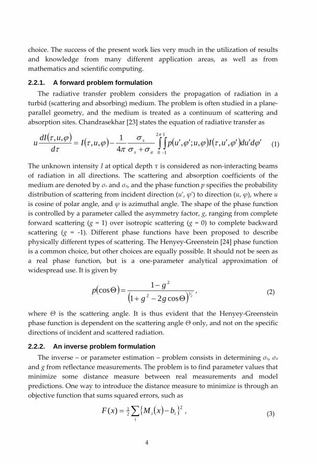
2.2.1. A forward problem formulation The radiative transfer problem considers the propagation of radiation in a
turbid (scattering and absorbing) medium. The problem is often studied in a planeparallel geometry, and the medium is treated as a continuum of scattering andabsorption sites. Chandrasekhar [23] states the equation of radiative transfer as
2
0
1
1
,,,;,41,,,, duduIuupuI
dudIu
as
s (1)
The unknown intensity I at optical depth is considered as non interacting beamsof radiation in all directions. The scattering and absorption coefficients of themedium are denoted by s and a, and the phase function p specifies the probabilitydistribution of scattering from incident direction (u , ) to direction (u, ), where uis cosine of polar angle, and is azimuthal angle. The shape of the phase functionis controlled by a parameter called the asymmetry factor, g, ranging from completeforward scattering (g = 1) over isotropic scattering (g = 0) to complete backwardscattering (g = 1). Different phase functions have been proposed to describephysically different types of scattering. The Henyey Greenstein [24] phase functionis a common choice, but other choices are equally possible. It should not be seen asa real phase function, but is a one parameter analytical approximation ofwidespread use. It is given by
23
cos21
1cos2
2
gggp , (2)
where is the scattering angle. It is thus evident that the Henyey Greensteinphase function is dependent on the scattering angle only, and not on the specificdirections of incident and scattered radiation.
2.2.2. An inverse problem formulation The inverse – or parameter estimation – problem consists in determining s, a
and g from reflectance measurements. The problem is to find parameter values thatminimize some distance measure between real measurements and modelpredictions. One way to introduce the distance measure to minimize is through anobjective function that sums squared errors, such as
iii bxMxF 2
21)( , (3)
5
where i denotes the respective measurement, and x is the vector of parameters tobe determined. Mi(x) are model predictions and bi are the correspondingmeasurements. An obvious formulation of the parameter estimation problem isthen
)(min xFx
. (4)
2.3. Solving a real industrial problem The work of the present thesis started as a real industrial problem – the
perceived need for a more detailed and more accurate model for light scattering inpaper and print. As is often the case with real life problems, not much wasspecified in advance, which meant equally large measures of freedom anduncertainty. Whether a new model could actually solve the perceived problems, orif solutions should be sought elsewhere, was unknown. Consequently, there wereno guidelines for what to incorporate in a new model, what approximations wouldbe acceptable, what accuracy was demanded or what methods to use.
A careful analysis of the industrial problem transferred it into a physicaldescription of the phenomena involved. This was then given a mathematicalformulation, and a detailed analysis led to numerical solution procedures forspecific sub problems. Turning to scientific computing made it possible to meetindustrial demands made on speed and stability. Implementation in computercode was then followed by analysis of accuracy and numerical performance. Thefinal software tool was evaluated through real industrial problems, and was finallyequipped with a graphical user interface for ease of use. The development of thecorresponding inverse solution procedures followed a similar path, and theforward and inverse software tools were eventually integrated.
The specific success of this work is to actually go all the way from a realindustrial problem via theoretical considerations from several different scientificand application areas to a working tool suitable for industrial use. An entirefinalized sequence of this kind is rarely seen in a thesis. An important part of thissuccess was constantly looking several steps ahead, and not solving each step inisolation. A lot of choices affect later steps, and if this is recognized the “right”choices can be made. The radiative transfer literature contains numerous examplesof problems that originate in failing to recognize this, which has without a doubtslowed down method development.
2.4. The resulting software tool The work presented in this thesis has resulted in the software tool DORT2002,
and its successful application to relevant paper industry problems is reportedelsewhere in the thesis. The name is an acronym for Discrete Ordinate Radiative
6
Transfer, where discrete ordinate is the name of the general solution strategy.However, there is a naming confusion since a number of such tools have beenpresented and several authors have named their tools DORT, which is simply shortfor problem type and solution strategy. Furthermore, since some of the presentedtools are poor, this has given the word DORT a bad reputation in some areas.Adding the year 2002 to the name is a way of distinguishing this particular tool.
It is concluded in this thesis that modern radiative transfer based solutionmethods like DORT2002 are now competitive in paper industry applications, andcould well replace Kubelka Munk for increased accuracy and understanding. Thegeneralization of light scattering modeling and reflectance measurementinterpretation provided by DORT2002 makes it in all aspects the Next GenerationKubelka Munk.
3. MATHEMATICAL AND NUMERICAL ESSENTIALS
3.1. More on the forward problem formulation Radiative transfer theory is a vast scientific area. Many different problem
formulations and solution strategies have been developed with different needs inmind. Historically, and in most frequent industrial use, is the 1D formulationwhich resolves the problem in one Cartesian coordinate (usually depth) and twoangular coordinates of spherical geometry. The 1D formulation is studied in thisthesis since it is a formulation of great industrial interest. Spatially resolved, i.e. 3D,formulations still need a breakthrough, as is briefly commented on in the sectionon future work.
Examples of solution strategies in use today are discrete ordinate methods(approximating integrals with numerical quadrature), methods using sphericalharmonics (orthogonal functions), methods using finite elements or finitedifferences, and Monte Carlo methods. Chandrasekhar described a method usingspherical harmonics [25], but later adopted the discrete ordinate method andfurther refined it [26]. Finite element and finite difference methods are morecompetitive in 3D problems, and Monte Carlo methods are very time consuming.Therefore, this work focuses exclusively on discrete ordinate methods.
Mudgett and Richards [27 28] described a discrete ordinate method for use intechnology and reported on numerical difficulties, as have many before and afterthem. These difficulties worsened when the use of computers made it possible totackle larger problems. It is only when the numerical difficulties are recognizedthat measures can be taken. A careful analysis of the problem makes it possible tofind such measures, and advances in numerical linear algebra and scientificcomputing provide ideas and software tools to make it a tractable problem.
7
The radiative transfer equation formulation (1) by Chandrasekhar is generallyused in 1D problems. This is also the formulation used in the present work.
3.2. Some details on the forward solution method The outline of the forward solution method is as follows. Fourier analysis gives
a system of equations, which are then discretized using numerical quadrature. Theinitial problem can then be transferred to a problem on eigenvalues of matrices.Boundary and continuity conditions are imposed, and the computed intensity isextended from the quadrature points to the entire interval through interpolationformulas.
The main steps to achieve a numerically stable solution procedure include; theFourier analysis with the evaluation of normalized associated Legendre functions,the discretization with the choice of numerical quadrature and the matrixformulation with the reduction of the eigenvalue problem, the preconditioning ofthe system of equations corresponding to the boundary and continuity conditions,and the avoidance of overflow in the solution and interpolation formulas. Therecognition of potential divide by zero situations and their reformulation is alsoimportant.
Several measures are taken to make the method fast. The N method and theintensity correction procedures allow high speed by maintaining accuracy at asignificantly lower number of terms in the quadrature formula than wouldotherwise be needed. Computational shortcuts stop the calculations earlier whencertain convergence criteria have been met. In addition, the sparse structure of thesystem of equations corresponding to the boundary and continuity conditionsshould be exploited.
Outlined below are some of the essential features of the forward solutionprocedure. The interested reader is referred to Paper I for details.
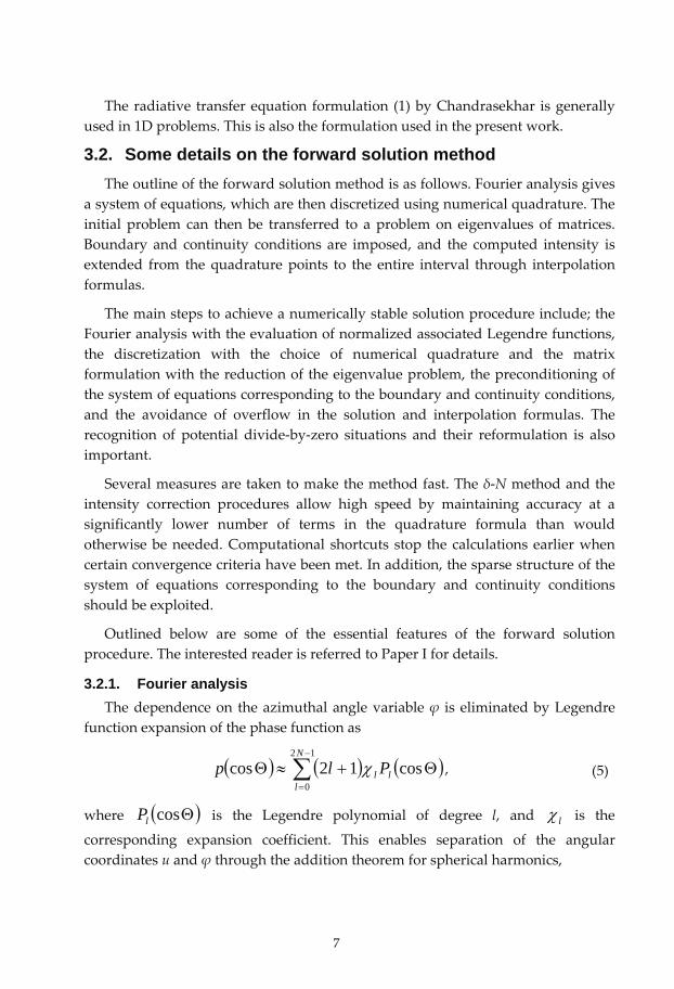
3.2.1. Fourier analysis The dependence on the azimuthal angle variable is eliminated by Legendre
function expansion of the phase function as12
0cos12cos
N
lll Plp , (5)
where coslP is the Legendre polynomial of degree l, and l is the
corresponding expansion coefficient. This enables separation of the angularcoordinates u and through the addition theorem for spherical harmonics,
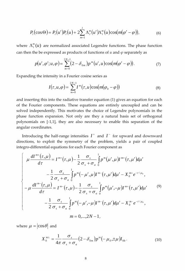
8
l
m
ml
mllll muuuPuPP
1cos2cos , (6)
where )(uml are normalized associated Legendre functions. The phase function
can then the be expressed as products of functions of u and separately as12
00 cos,2,;,
N
m
mm muupuup . (7)
Expanding the intensity in a Fourier cosine series as12
00cos,,,
N
m
m muIuI (8)
and inserting this into the radiative transfer equation (1) gives an equation for eachof the Fourier components. These equations are entirely uncoupled and can besolved independently. This motivates the choice of Legendre polynomials in thephase function expansion. Not only are they a natural basis set of orthogonalpolynomials on [ 1,1], they are also necessary to enable this separation of theangular coordinates.
Introducing the half range intensities I and I for upward and downwarddirections, to exploit the symmetry of the problem, yields a pair of coupledintegro differential equations for each Fourier component as
,,,21
,,21,,
,,,21
,,21,,
0
0
/0
1
0
1
0
/0
1
0
1
0
eXdIp
dIpId
dI
eXdIp
dIpId
dI
mmm
as
s
mm
as
smm
mmm
as
s
mm
as
smm
12,...,0 Nm ,
(9)
where cos and
bm
mas
sm IpX 0000 ,241
. (10)
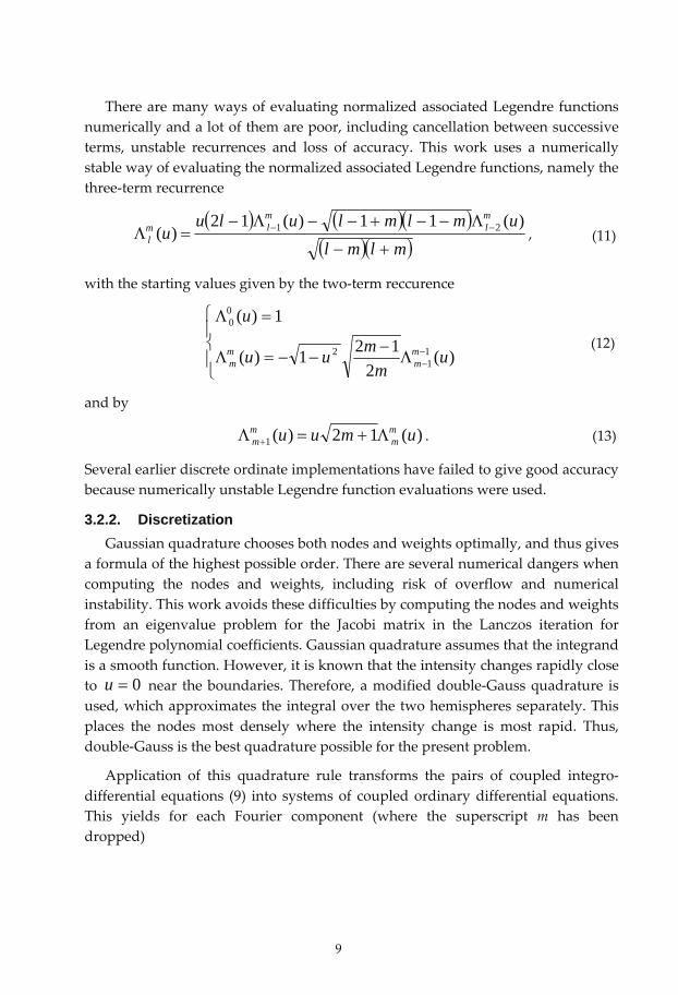
9
There are many ways of evaluating normalized associated Legendre functionsnumerically and a lot of them are poor, including cancellation between successiveterms, unstable recurrences and loss of accuracy. This work uses a numericallystable way of evaluating the normalized associated Legendre functions, namely thethree term recurrence
mlmlumlmlulu
uml
mlm
l)(11)(12
)( 21 , (11)
with the starting values given by the two term reccurence
)(2
121)(
1)(
11
2
00
um
muu
u
mm
mm
(12)
and by
)(12)(1 umuu mm
mm . (13)
Several earlier discrete ordinate implementations have failed to give good accuracybecause numerically unstable Legendre function evaluations were used.
3.2.2. Discretization Gaussian quadrature chooses both nodes and weights optimally, and thus gives
a formula of the highest possible order. There are several numerical dangers whencomputing the nodes and weights, including risk of overflow and numericalinstability. This work avoids these difficulties by computing the nodes and weightsfrom an eigenvalue problem for the Jacobi matrix in the Lanczos iteration forLegendre polynomial coefficients. Gaussian quadrature assumes that the integrandis a smooth function. However, it is known that the intensity changes rapidly closeto 0u near the boundaries. Therefore, a modified double Gauss quadrature isused, which approximates the integral over the two hemispheres separately. Thisplaces the nodes most densely where the intensity change is most rapid. Thus,double Gauss is the best quadrature possible for the present problem.
Application of this quadrature rule transforms the pairs of coupled integrodifferential equations (9) into systems of coupled ordinary differential equations.This yields for each Fourier component (where the superscript m has beendropped)
10
,,,21
,,21,
,
,,,21
,,21,
,
0
0
/0
1
1
/0
1
1
eXIp
IpId
dI
eXIp
IpId
dI
i
N
jjijj
as
s
N
jjijj
as
si
ii
i
N
jjijj
as
s
N
jjijj
as
si
ii
Ni ,...,1 .
(14)
This can now be put in block matrix form as
II
II
dd
, (15)
where the , and Q are defined in Paper I. It is well known that the
homogenous solutions are of the form kegI , which gives the NN 22homogeneous eigenvalue problem
gg
gg
k (16)
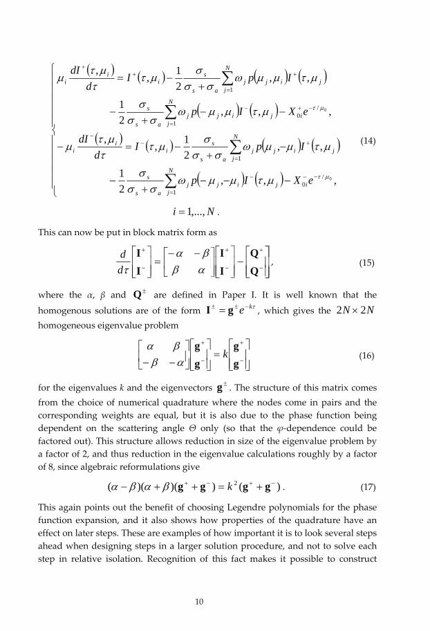
for the eigenvalues k and the eigenvectors g . The structure of this matrix comesfrom the choice of numerical quadrature where the nodes come in pairs and thecorresponding weights are equal, but it is also due to the phase function beingdependent on the scattering angle only (so that the dependence could befactored out). This structure allows reduction in size of the eigenvalue problem bya factor of 2, and thus reduction in the eigenvalue calculations roughly by a factorof 8, since algebraic reformulations give
)())()(( 2 gggg k . (17)
This again points out the benefit of choosing Legendre polynomials for the phasefunction expansion, and it also shows how properties of the quadrature have aneffect on later steps. These are examples of how important it is to look several stepsahead when designing steps in a larger solution procedure, and not to solve eachstep in relative isolation. Recognition of this fact makes it possible to construct
11
numerically efficient solution procedures, and ignorance of this fact has broughtabout unstable procedures and slowed development over the years.
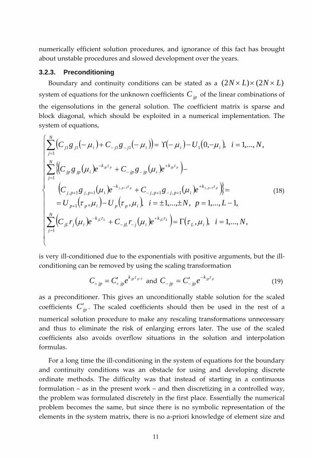
3.2.3. Preconditioning Boundary and continuity conditions can be stated as a )2()2( LNLN
system of equations for the unknown coefficients jpC of the linear combinations of
the eigensolutions in the general solution. The coefficient matrix is sparse andblock diagonal, which should be exploited in a numerical implementation. Thesystem of equations,
,,...,1,,
,1,...,1,,...,1,,,
,,...,1,,0
1
1
1,1,1,1,
1
11
1111
1,1,
NierCerC
LpNiUUegCegC
egCegC
NiUgCgC
iL
N
j
kijjL
kijjL
ippipp
kipjpj
kipjpj
N
j
kijpjp
kijpjp
ii
N
jijjijj
LjLLjL
ppjppj
pjppjp
(18)
is very ill conditioned due to the exponentials with positive arguments, but the illconditioning can be removed by using the scaling transformation
1pjpkjpjp eCC and pjpk
jpjp eCC (19)
as a preconditioner. This gives an unconditionally stable solution for the scaledcoefficients jpC . The scaled coefficients should then be used in the rest of a
numerical solution procedure to make any rescaling transformations unnecessaryand thus to eliminate the risk of enlarging errors later. The use of the scaledcoefficients also avoids overflow situations in the solution and interpolationformulas.
For a long time the ill conditioning in the system of equations for the boundaryand continuity conditions was an obstacle for using and developing discreteordinate methods. The difficulty was that instead of starting in a continuousformulation – as in the present work – and then discretizing in a controlled way,the problem was formulated discretely in the first place. Essentially the numericalproblem becomes the same, but since there is no symbolic representation of theelements in the system matrix, there is no a priori knowledge of element size and
12
no obvious way to symbolically construct a useful preconditioner. This actuallyslowed development in the area for decades, and was the main reason that discreteordinate methods were considered numerically intractable.
3.3. More on the inverse problem formulation There are plenty of rather crude methods for estimating only the scattering and
absorption parameters for turbid media, and most of them use very approximateforward problems. Methods for estimating the asymmetry factor as well are scarce,and even fewer are efficient and accurate. Most efforts come from medicalapplications, while industry has shown less interest so far. Reported methods areapproximate, use inflexible boundary conditions or have difficulties findingsuitable starting points [29 30]. Very long computation times are also a frequentproblem [31].
Estimating only the scattering and absorption parameters from reflectancemeasurements is straightforward in cruder two flux problem formulations likeKubelka Munk. However, more accurate estimation of an extended number ofparameters is an outstanding issue in more general radiative transfer problemformulations. In this work, the radiative transfer problem has an angle resolvedformulation, and a many flux solution procedure is used. The parameterestimation problem is formulated as a least squares optimization problem, and atwo phase method for its solution is implemented and evaluated. The successfulrecovery of s, a and g is illustrated by application to relevant paper industryproblems.
The two phase method uses two problem formulations that apply to both theforward and the inverse settings. The full problem comprises angle resolved data(intensity measurements in chosen directions) together with scattering, absorptionand asymmetry parameters. The simpler d/0 problem involves standardizedreflectance factor data as used in the paper industry, and scattering and absorptionparameters only. How to handle anisotropy is a new and open question for thepaper industry, and refined measurement and simulation methods are needed toresolve this matter. This work is a step in that direction.
The parameter estimation problem (4) is to find parameter values that minimizesome distance measure between real measurements and model predictions. In thiswork, this is done through an objective function (3) that sums squared errors, andthe parameter estimation problem is given an explicit least squares formulation.This formulation is statistically optimal if the measurement errors are normallydistributed, which may reasonably be considered to be the case here.
13
3.4. Some details on the inverse solution method The obvious way to attack the full parameter estimation problem would be to
find a suitable starting point and simply apply a standard optimization method.However, it turns out that the character of the full problem makes it very sensitiveto the choice of starting point. In fact, in most cases the optimization methods donot converge unless the starting point is very close to the optimum. Unfortunately,there is no simple way to devise a starting point for the full problem. On thecontrary, while s and a may be approximated with simpler models, g isinaccessible and yet is essential for convergence. Therefore, a direct attack on thefull problem seems unfeasible.
However, since the simpler d/0 problem is more well behaved, and since g is afree parameter there, it should be possible to parameterize that case and run ascalar optimization on g to find a suitable starting point. This also relieves the userof having to supply an initial value of g through guesswork, and withoutknowledge. Thus, a two phase approach should be viable.
The solution procedure to the inverse d/0 problem actually provides aparameterization, giving s(g) and a(g), see Paper VI for details. Using thisparameterization, the objective function of the full problem can be evaluated fromthe single scalar parameter g. Of course, this only spans a curve in the parameterspace, so a solution to the full problem can not be expected. However, it is likelythat this curve passes the solution close enough to provide a good starting point.This starting point is given by the solution to a scalar optimization problem over g,using the objective function of the full problem and the parameterizationmentioned above. Preferably, the scalar optimization problem should be solvedcheaply. Since g is limited to the interval ] 1,1[ and the highest accuracy is notneeded, a derivative free golden section search method with a relaxed convergencecriterion can be used. Thanks to the special parameterization and scalaroptimization in the first phase, the starting point for the second phase is nowalready close to the optimum. This makes it possible to use a simple andstraightforward Gauss Newton method for the second phase and still expect goodconvergence properties.
Thus, this two phase solution method for the full parameter estimation problemgives fast convergence and accurate results, although it is only based on simpleand straightforward optimization methods. It is the intelligent construction of thetwo phases that avoids poor efficiency or accuracy and that also provides a verygood starting point without guesswork from the user, which in itself is a greatproblem in many applications.
14
To the author s knowledge the kind of two phase approach for the inverseradiative transfer problem presented in this work has not been published before. Itis not uncommon to first estimate s and a from some measurements and anassumption or guess of g, and then use these parameter values as the starting pointfor the full problem. However, this is far from optimal, since the values of s and a
are fixed from the more or less ad hoc choice of g. That first step merely ensuresthat the triplet s, a and g is compatible. No use is made of the full problem or therest of the measurements when obtaining the starting point; instead, the startingpoint and the rest of the problem are treated completely separately. The first phasesuggested here actually manages to find the best (in some aspect) starting point byactually combining – through the parameterization – the simpler d/0 problem withthe objective function of the full problem, thus also utilizing all measurements.
4. A SHORT TOUR THROUGH THE PAPERS
The papers in this thesis cover the radiative transfer problem from differentperspectives. Both the forward and the inverse problems are treated, and fromboth a mathematical and an applied point of view. Table 1 groups the papers basedon their main focus.
Table 1. The papers in the thesis, grouped in categories based on their main focus.
Mathematics Application
Forward Paper I
Paper II
Paper III
Paper IV
Inverse Paper V
Paper VI
Paper VII
Paper I presents a radiative transfer problem formulation, and goes through allthe steps necessary to get a fast and numerically stable solution procedure. Thesoftware tool DORT2002, based on these steps, is suggested for light scatteringsimulations in paper and print, but also as a general tool for radiative transferproblems. Its modularized design and ability to give any kind of intermediateresults and performance data required also allows for methodical numericalexperiments. The accuracy is verified by application to different sets of testproblems.
Paper II gives a systematic presentation of the effect of the steps that are neededor are possible to make any discrete ordinate radiative transfer solution methodnumerically efficient. This is done through studies of the numerical performance of
15
the stability enhancing and speed increasing steps used in modern discreteordinate radiative transfer algorithms. It is shown how different measures, basedon both mathematical reformulations and physical insight, together give anunconditionally stable solution procedure to a problem previously considerednumerically intractable, and how they together decrease the computation timecompared to a naive implementation by a factor of 1 000 – 10 000 in typical casesand by a factor up to and beyond 10 000 000 in extreme cases.
Paper III argues that in many cases modern solution methods from radiativetransfer theory could be considered for increased understanding of paper optics,and a comprehensive list of advantages for the applied user is supplied. Thecoefficients of DORT2002 and Kubelka Munk are compared, and some of thedifferences when applying these models are quantified. It is noted that even in thetheoretically ideal case of perfectly diffuse illumination and perfectly isotropicsingle scattering process, the light intensity inside and outside the sample is notperfectly diffuse. This is in opposition to what one would intuitively expect, andviolates the assumptions of the Kubelka Munk model. It is shown that this cancause large errors in Kubelka Munk reflectance calculations, and that themagnitude of the error shows a strong dependence on the degree of absorption,with higher absorption giving greater error.Paper IV analyzes the anomalous dependence between the scattering and
absorption coefficients in the Kubelka Munk model for strongly absorbingsamples. Errors in Kubelka Munk are quantified, using DORT2002 and totalreflectance data. It is recognized that anisotropy in the reflected light will affectthese results, and it is suggested that both instrument geometry and surfaceroughness should be included in future studies.
Paper V presents two Levenberg Marquardt methods for parameter estimationin the radiative transfer problem. A feasible path approach and an SQP typemethod are analyzed and compared. It is shown that the feasible path approach isadvantageous when estimating a small number of parameters, whereas the SQPtype method is more efficient when a large number of parameters are to beestimated. A sensitivity analysis is performed, and it is shown how it can be usedfor designing measurements with minimal impact from measurement noise. Theinfinite dimensional formulation of the parameter estimation problem allows forthe application of functional analysis and thereby for future theoretical studies ofthe existence and uniqueness of solutions.
Paper VI presents a finite dimensional two phase approach for parameterestimation in the radiative transfer problem. While finding a feasible starting pointcan in itself be a great problem in many applications, the first phase suggested hereactually manages to find the best (in some aspect) starting point by combining –through a parameterization – a simpler problem with the objective function of the
16
full problem. The first phase efficiently provides a very good starting point for thesecond phase, for which a simple and straightforward Gauss Newton methodgives fast convergence and accurate results. The successful recovery of scattering,absorption and asymmetry parameters by this two phase method is illustrated byapplication to relevant paper industry problems. The character of the illconditioned parameter estimation problem is investigated, and a sensitivityanalysis is performed. It is noted that radiative transfer based solution methodslike DORT2002 are now competitive in paper industry applications, and could wellreplace Kubelka Munk for increased understanding.
Paper VII uses radiative transfer theory to examine the recently suggested socalled revised Kubelka Munk (Rev KM) theory [20], and thereby comments on thevalidity of different modeling strategies and their combinations. More specifically,the inclusion of the so called scattering induced path variation factor in the endresults is inspected. Theoretical arguments show that properties in Rev KM areinadequately derived, and that the scattering induced path variation factor cannotbe used together with a differential model as proposed. In Rev KM, properties arederived using finite layers, and are then inadequately— without going through alimiting process—used in relations that are explicitly obtained using infinitesimallayers. Simulation experiments show that Rev KM yields significant errors inpredicted mixture reflectances, i.e. it is not accurate, and that it is clearly not selfconsistent. The absorption is noticeably overestimated by Rev KM, and in no caseis the model better than the original Kubelka Munk.
Papers I III and VI VII are the result of own work, while Papers IV V are theresult of cooperation. The contribution of the author of this thesis to Paper IVconsists in developing simulation tools, performing simulations, interpreting andpresenting simulation results, and partly writing the paper. The contribution of theauthor of this thesis to Paper V consists in developing simulation tools regardingaccuracy and forward modeling, designing numerical experiments, interpretingand presenting simulation results, and partly writing the paper.
5. A PATH TO PROBLEM INSIGHT
Early in this work, people talked about the errors in the Kubelka Munk model,and the literature confirmed that there were anomalies. The first and naturalreaction to this was that if the model is erroneous, a correct – or at least better – oneshould be devised. Indeed, many “corrections” and “extensions” had beensuggested for handling various individual aspects of the reported anomalies, butnone convincingly handled all aspects. Since Kubelka Munk is a very simple and
17
approximate “two flux” model for the radiative transfer problem, it wasreasonable to seek a more general and accurate “many flux” model. KubelkaMunk would then be included as the simplest special case, which is an appealingway to generalize a model.
The development of a discrete ordinate solution procedure started. Severalnumerical challenges were met, and finally the software tool DORT2002 wasimplemented. With this accurate angle resolved solution procedure, it was nolonger necessary to hold on to many of the assumptions of the Kubelka Munkmodel. On the contrary, the new solution procedure could easily incorporate theactual conditions of the measurement device, such as illumination and detectiongeometry (the d/0° instrument geometry that is standardized in the paper industrywas used). It turned out that some of the actual conditions could be far from thepostulated assumptions, even in idealized cases. One example is the illuminationthat – due to the gloss trap – is not perfectly diffuse.
However, the largest deviation was not expected. It turned out that even inidealized cases the light distribution would not be perfectly diffuse, which is themain assumption in the Kubelka Munk model. Even in a simulated idealizedsituation with a perfectly diffuse illumination and a perfectly isotropic singlescattering process, the reflected light would be anisotropic, with more lightreflected in large polar angles. The situation would become even worse whenincluding the effect of the gloss trap, or when using highly absorbing or opticallythin media.
It was now apparent that the reported errors were not caused exclusively by theKubelka Munk model. A large contribution to the errors lies in the idealized viewof both model and instrument. The Kubelka Munk model is valid under certainassumptions, and the d/0 instrument is designed to realize those assumptions (asfar as possible). The errors occur when the model and the instrument are usedtogether as if though the assumptions were indeed met. This is not easy to see,since some assumptions are implicit. One example is the detection, which viewsthe sample in a narrow solid angle around the normal to the sample. Since oneassumption is that all light is perfectly diffuse, it is thus implicitly assumed that thereflected light intensity in all other angles equals the one detected in the normaldirection. Since more light, as noted above, is always reflected in large polarangles, the detected intensity is an underestimation. Further, the underestimationdepends nonlinearly on the absorption and optical thickness of the sample, and isnot possible to detect within the measurement system. This underestimation thenpropagates throughout the Kubelka Munk model, and affects the computedresults. Some of the errors thus originate from the fact that instrument readings are
18
incorrectly interpreted, which is due to false assumptions on the measurementsituation and not to the model used.
This insight led to a more combined view of the measurement system. Themeasurement device and the simulation model cannot be viewed as separateinstances, which is a widespread implicit practice in applied reflectancemeasurements. Rather, given a measurement device, measurement data should beinterpreted through a (sufficiently accurate) model that takes into consideration theactual geometry and function of the instrument. DORT2002 could straightforwardlytake this into account. It was now easily shown how the standardized use ofKubelka Munk and the d/0 instrument leads to errors, and that the errors arisingfrom an over idealized view of the instrument could be larger than any errorsinherent in the Kubelka Munk model itself.
During these investigations, it was natural to look more closely into the detailsof the actual function of the instrument. It is not entirely obvious how theinstrument transforms detector readings into output data. Apart from geometricalconsiderations of illumination and detection, the calibration itself plays a vital role.This led to an even more combined view of the measurement system. Not onlyshould the measurement device and the simulation model be viewed as a unitrather than as separate instances, the actual calibration routine should also beincluded in the interpretation of measurement data. It is also possible to includethis in DORT2002. It has not been used on applied problems yet, but it will be anatural part in future work. In principle, it would be possible to include the entirecalibration hierarchy, but this is not likely to give a lot more accuracy, sincedifferent and more accurate instruments are used there.
5.1. What is ‘correct’ is relative to the assumptions made Papers III and IV use an idealized view of the instrument, and no actual
measurement conditions are included in the interpretation of measurement data.Papers VI and VII – written with deeper insight – recognize the non idealproperties of the instrument and include them in the interpretation ofmeasurement data. In none of the papers in this thesis is the calibration of theinstrument in the interpretation of measurement data also included.
It can be argued that numerical results from Papers III and IV are correct withthe assumption of idealized instruments, which is also a widespread implicitassumption in applied reflectance measurements. It can simultaneously be arguedthat numerical results from Papers VI and VII are more accurate, since they takethe actual geometry and function of the instrument into consideration in theinterpretation of measurement data. If papers III and IV were written today, theyalso would take this into account. Their reasoning and conclusions would still
19
hold, but some numerical results would be different – and more accurate. Futurework will be made even more accurate by also including the instrumentcalibration.
The question of whether or not the results are correct is not absolute, butrelative to the assumptions made. If the assumptions are explicitly stated, resultscan be said to be correct within those assumptions. If assumptions are implicitly –or even unconsciously – used, this may lead to severe errors. If the goal is to get asclose as possible to a true physical quantity, there is no question that the entiremeasurement system should be included in the greatest possible detail in theinterpretation of measurement data. In that case it can be objectively said that oneresult is more correct than the other.
6. ANISOTROPIC REFLECTANCE
In the process of including instrument geometry in the interpretation ofmeasurement data, work on a master’s thesis [32] was supervised. It led tointeresting results, and the extended work will be reported elsewhere. However, ashort summary is appropriate here.
How the anisotropy of light reflected from paper depends on the paperabsorption and thickness was investigated experimentally and theoretically. Thiswas done by measuring the angular resolved reflectance from a series ofhandsheets containing different amounts of dye and filler and varying ingrammage. Measurements and simulations both showed that the anisotropyincreases with increased absorption and is higher for lower grammages. Therelative amount of light scattered into larger polar angles increases for these cases.It was also shown that the reflectance from what is intuitively thought to be aperfect diffusor strongly depends on the illumination conditions, meaning that abulk scattering medium that reflects light diffusely independently of theillumination conditions actually does not exist.
How the anisotropy affects d/0 instrument measurements was examined.DORT2002 gave access to the objective scattering and absorption parameters (notonly the model and geometry dependent Kubelka Munk coefficients) through aninstrument originally not designed for this purpose. It turned out that even inidealized cases the light distribution would not be perfectly diffuse, which is themain assumption in the Kubelka Munk model. The situation would become evenworse when including the effect of the gloss trap, or when using highly absorbingor optically thin media. It was shown that this can explain more than half of thewidely investigated anomalous parameter dependencies of the Kubelka Munkmodel.
20
The causes of anisotropic reflectance were investigated and it was shown that itdepends on the relative contribution from near surface bulk scattering. Thereflectance in larger polar angles is higher from near surface bulk scattering than itis from scattering deeper inside the medium. Near surface bulk scatteringdominates in strongly absorbing media since the remaining light is absorbed, andin optically thin media since the remaining light is transmitted. Obliquely incidentillumination causes the light to scatter closer to the surface, and this also causes therelative contribution from near surface bulk scattering to increase.
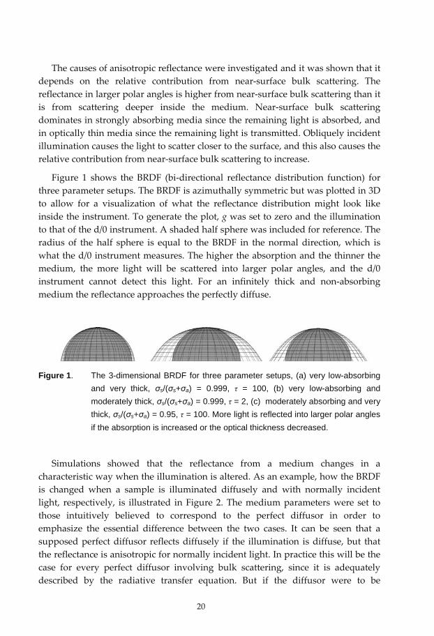
Figure 1 shows the BRDF (bi directional reflectance distribution function) forthree parameter setups. The BRDF is azimuthally symmetric but was plotted in 3Dto allow for a visualization of what the reflectance distribution might look likeinside the instrument. To generate the plot, g was set to zero and the illuminationto that of the d/0 instrument. A shaded half sphere was included for reference. Theradius of the half sphere is equal to the BRDF in the normal direction, which iswhat the d/0 instrument measures. The higher the absorption and the thinner themedium, the more light will be scattered into larger polar angles, and the d/0instrument cannot detect this light. For an infinitely thick and non absorbingmedium the reflectance approaches the perfectly diffuse.
Figure 1. The 3-dimensional BRDF for three parameter setups, (a) very low-absorbing and very thick, s/( s+ a) = 0.999, τ = 100, (b) very low-absorbing and moderately thick, s/( s+ a) = 0.999, τ = 2, (c) moderately absorbing and very thick, s/( s+ a) = 0.95, τ = 100. More light is reflected into larger polar angles if the absorption is increased or the optical thickness decreased.
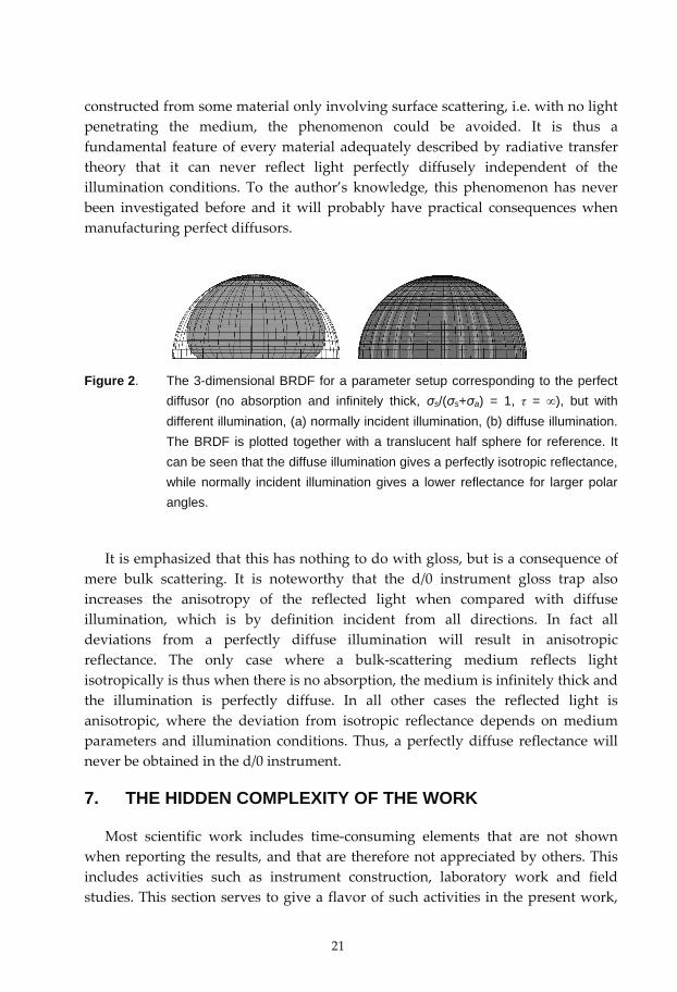
Simulations showed that the reflectance from a medium changes in acharacteristic way when the illumination is altered. As an example, how the BRDFis changed when a sample is illuminated diffusely and with normally incidentlight, respectively, is illustrated in Figure 2. The medium parameters were set tothose intuitively believed to correspond to the perfect diffusor in order toemphasize the essential difference between the two cases. It can be seen that asupposed perfect diffusor reflects diffusely if the illumination is diffuse, but thatthe reflectance is anisotropic for normally incident light. In practice this will be thecase for every perfect diffusor involving bulk scattering, since it is adequatelydescribed by the radiative transfer equation. But if the diffusor were to be
21
constructed from some material only involving surface scattering, i.e. with no lightpenetrating the medium, the phenomenon could be avoided. It is thus afundamental feature of every material adequately described by radiative transfertheory that it can never reflect light perfectly diffusely independent of theillumination conditions. To the author’s knowledge, this phenomenon has neverbeen investigated before and it will probably have practical consequences whenmanufacturing perfect diffusors.
Figure 2. The 3-dimensional BRDF for a parameter setup corresponding to the perfect diffusor (no absorption and infinitely thick, s/( s+ a) = 1, τ = ∞), but with different illumination, (a) normally incident illumination, (b) diffuse illumination. The BRDF is plotted together with a translucent half sphere for reference. It can be seen that the diffuse illumination gives a perfectly isotropic reflectance, while normally incident illumination gives a lower reflectance for larger polar angles.
It is emphasized that this has nothing to do with gloss, but is a consequence ofmere bulk scattering. It is noteworthy that the d/0 instrument gloss trap alsoincreases the anisotropy of the reflected light when compared with diffuseillumination, which is by definition incident from all directions. In fact alldeviations from a perfectly diffuse illumination will result in anisotropicreflectance. The only case where a bulk scattering medium reflects lightisotropically is thus when there is no absorption, the medium is infinitely thick andthe illumination is perfectly diffuse. In all other cases the reflected light isanisotropic, where the deviation from isotropic reflectance depends on mediumparameters and illumination conditions. Thus, a perfectly diffuse reflectance willnever be obtained in the d/0 instrument.
7. THE HIDDEN COMPLEXITY OF THE WORK
Most scientific work includes time consuming elements that are not shownwhen reporting the results, and that are therefore not appreciated by others. Thisincludes activities such as instrument construction, laboratory work and fieldstudies. This section serves to give a flavor of such activities in the present work,
22
specifically of algorithm development and implementation, but also of vastamounts of algebraic details.
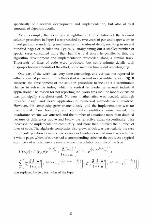
As an example, the seemingly straightforward presentation of the forwardsolution procedure in Paper I was preceded by two years of pen and paper work ininvestigating the underlying mathematics to the utmost detail, resulting in severalhundred pages of calculations. Typically, straightening out a smaller number ofspecial cases consumed more than half the total effort. In parallel to this, thealgorithm development and implementation proceeded along a similar track.Thousands of lines of code were produced, but some minute details tookdisproportionate amounts of the effort, not to mention time spent on debugging.
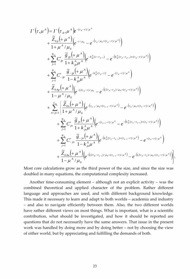
One part of the work was very time consuming, and yet was not reported ineither a journal paper or in this thesis (but is covered in a scientific report [33]). Itconcerns the development of the solution procedure to include a discontinuouschange in refractive index, which is central in modeling several industrialapplications. The reason for not reporting that work was that the model extensionwas principally straightforward. No new mathematics was needed, althoughphysical insight and clever application of numerical methods were involved.However, the complexity grew tremendously, and the implementation was farfrom trivial. New boundary and continuity conditions were needed, thequadrature scheme was affected, and the number of equations more than doubledbecause of differences above and below the refractive index discontinuity. Thisincreased the implementation complexity, and more than doubled the number oflines of code. The algebraic complexity also grew, which was particularly the casefor the interpolation formulas. Earlier one or two liners would now cover a half toa whole page, which of course had a corresponding effect on the code. As a typicalexample – of which there are several – one interpolation formula of the type
N
j
k
j
jj
kk
j
jj
b
bbj
btbjtj
bbb
eek
gCee
kg
C
eeZ
eII
1
)()()(
//
0
0
1
~
1
~/1
~,,
00
was replaced by two formulas of the type
23
./1
~1
~1
~/1
~/1
~1
~1
~/1
~,,
/)(/)2(/)(/)2(
0
0
1
/)(/)()(
1
/)()(/)(
1
/)(//)(/
0
0
/)(/)2(/)2(
0
0
1
/)()(
1
/)()()(
/)(//
0
0
/)(
0101
11
11
0101
00
11
00
AnnA
AnnA
A An
Annn
Ajn
A Annn
Ajn
An
A Ann
Ann
AppAA
A App
Ajp
A Appp
Ajpp
Ajp
App
AA
eeZ
eek
gC
eek
gC
eeZ
eeZ
eek
gC
eek
gC
eeZ
eII
A
AAn
N
j
kAA
jn
Ajn
jn
N
j
kAA
jn
Ajn
jn
L
pnA
An
A
AAp
N
j
kAA
jp
Ajp
jp
N
j
kkAA
jp
Ajp
jp
A
Ap
AA
A
Most core calculations grow as the third power of the size, and since the size wasdoubled in many equations, the computational complexity increased.
Another time consuming element – although not an explicit activity – was thecombined theoretical and applied character of the problem. Rather differentlanguage and approaches are used, and with different background knowledge.This made it necessary to learn and adapt to both worlds – academia and industry– and also to navigate efficiently between them. Also, the two different worldshave rather different views on most things. What is important, what is a scientificcontribution, what should be investigated, and how it should be reported arequestions that do not necessarily have the same answers. That issue in the presentwork was handled by doing more and by doing better – not by choosing the viewof either world, but by appreciating and fulfilling the demands of both.
24
8. DISCUSSION
A problem formulation and a solution method were outlined for the forwardradiative transfer problem in multilayer scattering and absorbing media usingdiscrete ordinate model geometry. First, all necessary steps to get a numericallystable solution procedure were treated, and then methods were introduced toincrease the speed by a factor of several thousands or millions compared to a naiveapproach. The method was shown to be unconditionally stable, though theproblem was previously considered numerically intractable. Systematic studies ofthe numerical performance of the stability enhancing and speed increasing stepsused in modern tools like DORT2002 illustrate the effect of the steps that are neededor possible to make any discrete ordinate radiative transfer solution methodnumerically efficient.
It was argued that modern radiative transfer based solution methods likeDORT2002 are now competitive in paper industry applications, and could well beconsidered instead of the Kubelka Munk model for increased understanding of theoptics of paper and print. It was shown that Kubelka Munk is a simple special caseof DORT2002, and the two models and their coefficients were compared. It wasnoted that the light distribution deviates from the perfectly diffuse even under thetheoretically ideal conditions for which Kubelka Munk was created, and that themagnitude of the error shows a strong dependence on the degree of lightabsorption, with higher absorption giving greater error. It was also noted that thiseffect can cause large errors in Kubelka Munk reflectance calculations, and thatthis partly explains the anomalous dependence between the scattering andabsorption coefficients in the Kubelka Munk model for strongly absorbingsamples. This intrinsic error in the Kubelka Munk model was mapped bycomparing light scattering calculations with the more accurate DORT2002. It wasfurther recognized that anisotropy in the reflected light will affect these results,and it was suggested that both instrument geometry and surface roughness shouldbe included in future studies.
The inverse radiative transfer problem was given a least squares formulation.Two Levenberg Marquardt methods, a feasible path approach and an SQP typemethod, were analyzed and compared. A sensitivity analysis was given, and it wasshown how it can be used for designing measurements with minimal impact ofmeasurement noise. Numerical experiments were performed to exemplify theusefulness of the theory. This formulation of the parameter estimation problem canalso be useful in future functional analytic studies of existence and uniqueness.
A two phase method for estimation of the scattering and absorption coefficientsand the asymmetry factor ( s, a and g) in the radiative transfer problem was
25
presented. The first phase parameterizes s and a through g via a simplified modeland performs – at a relatively low cost – a scalar optimization over g. It was shownthat this gives such a good starting point that the second phase can be accuratelyperformed by a simple Gauss Newton method. The parameter estimation problemwas shown to be non trivial and ill conditioned, and that standard optimizationmethods are so sensitive to the choice of starting point for this problem that it ishard to find a starting point that gives convergence at all was discussed. The newtwo phase method was illustrated by application to relevant paper industryproblems, and efficiency and sensitivity measures were given.
The revised Kubelka Munk model was examined theoretically andexperimentally, and comments were made on the validity of different modelingstrategies and their combinations. Systems of dyed paper sheets were simulated,and the results were compared with other models. The results showed that therevised Kubelka Munk model yields significant errors in predicted dye papermixture reflectances, and is not self consistent. The absorption is noticeablyoverestimated. Theoretical arguments showed that properties in the revisedKubelka Munk model are inadequately derived. The main conclusion was that therevised Kubelka Munk model is wrong in using the so called scattering inducedpath variation factor together with a differential model as proposed. Consequently,the model should not be used for light scattering calculations. Instead, the originalKubelka Munk model should be used where its accuracy is sufficient, and aradiative transfer tool of higher resolution should be used where higher accuracy isneeded.
It was shown how the standardized use of Kubelka Munk and the d/0instrument leads to errors, and that the errors arising from an over idealized viewof the instrument – due to the fact that instrument readings are incorrectlyinterpreted – could be larger than any errors inherent in the Kubelka Munk modelitself. It was argued that the measurement device and the simulation model cannotbe viewed as separate instances, which is a widespread implicit practice in appliedreflectance measurements. Rather, given a measurement device, measurement datashould be interpreted through a (sufficiently accurate) model that takes intoconsideration the actual geometry, function and calibration of the instrument.DORT2002 can do this, and it was described how this gives access to objectivescattering and absorption parameters, and that this can better explain theanomalous parameter dependence of the Kubelka Munk model.
How this work started in a real industrial problem and then went all the wayvia theoretical considerations from several different scientific and application areasto a working tool suitable for industrial use was discussed. This tool, DORT2002, is
26
in all aspects the Next Generation Kubelka Munk. It provides greater range ofapplicability, higher accuracy and increased understanding. Several perceivedproblems with Kubelka Munk have been or can be explained. It offers betterinterpretation of measurement data, and facilitates the exchange of data betweenthe paper and graphic arts industries. It opens up for understanding of anisotropicreflectance and for the utilization of the asymmetry factor to design anisotropy,and thereby for the design of different visual appearance or optical performance innew printed or paper products.
The understanding of the numerical difficulties in the forward and inverseradiative transfer problems has been advanced, and efficient solution procedureshave been presented. This is a substantial contribution to the area of numericalsolutions of integro differential equations and their inverse, including theoreticalperturbation results.
9. FUTURE WORK
The work presented in this thesis has led to a number of interesting questionsand areas of future research. Some work has already started or is planned, whilesome lies further in the future or is left for others to pursue.
On the more theoretically mathematical side, it has been noted that not much isknown about the existence and uniqueness of solutions to the forward or to theinverse radiative transfer problem. A functional analytic approach would find arich research area here. Since the use of models of this type is growing rapidly invarious applied sciences, studies of this kind are called for.
Spatially resolved radiative transfer models and corresponding forward andinverse solution algorithms are interesting within both mathematics and appliedsciences. Theoretically, even less is known here, and applications need morepowerful tools than the rather crude finite element methods in use today. Variousimaging, localizing, characterizing and optimizing problems in most areas whereradiative transfer is used today would greatly benefit from a breakthrough here.
Monte Carlo models are becoming more frequently used in the same areas asradiative transfer models. Although they are much slower and often have a largenumber of parameters that are not easily determined, the development of fastercomputers will make them increasingly interesting. Furthermore, the possibility toinclude any desired phenomena, to avoid undesired approximations and to usephysical rather than phenomenological parameters, gives Monte Carlo modelspotentially great explanative power. There are ongoing activities in this area. Anoutstanding problem then is parameter estimation in Monte Carlo models. Their
27
genuinely discrete nature and their long computation times are an obstacle for fulluse in applied sciences.
Looking more specifically at the paper optics area, it has been noted that thereare at least two key areas that need more modeling development. One isfluorescence phenomena, which have a large impact on visual appearance andcolor reproduction. Yet, the treatment of fluorescence in standards, practice andmodels is varying, poor or non existent. The other area is surface roughness andgloss, which also have a large impact on visual appearance. Although severalattempts have been made to model this, a lot remains to be done to fullyunderstand and describe surface scattering and to distinguish it from bulkscattering.
The discontinuous change in refractive index between the surrounding air andan ink covered paper gives rise to refraction and total reflection. Today this isapproximately handled for d/0 geometry with Kubelka Munk and the so calledSaundersson correction, using a coefficient whose value is debated. DORT2002handles the refractive index change in any geometry without approximations andwithout any unknown coefficient. Work is planned to compare DORT2002, MonteCarlo simulations and Kubelka Munk with the Saundersson correction, with realmeasurements for evaluation.
The anisotropic scattering from paper and other turbid media is a newlydiscovered phenomenon. The causes are only just understood and work is inprogress to present this. The consequences of this anisotropy for applications alsoneed investigation. Ongoing activities use DORT2002 to simulate the actualfunction and geometry of different reflectance measurement instruments in thepaper industry, to more correctly interpret measurement data. Other activities lookat standardization issues and the non compatibility between d/0 and 45/0instruments, in order to facilitate the exchange of data between the paper andgraphic arts industries.
Very little is written and known about numerical values of the asymmetryfactor for materials like paper, and the question of anisotropy and the utilization ofthe asymmetry factor is new to the paper industry. Spectral goniophotometermeasurements of various paper samples are planned for a broad evaluation of thenew parameter estimation methods for the asymmetry factor, but also of thespectral dependence and the numerical values of the asymmetry factor.
While DORT2002 is a generalization of Kubelka Munk, and it has already beenargued that DORT2002 could replace Kubelka Munk for increased accuracy andunderstanding, it would be possible to generalize the whole system. This wouldmean replacing Kubelka Munk with DORT2002, but it also has other implications. It
28
would mean replacing (or complementing) d/0 measurements with angle resolvedmeasurements (or at least with measurements in more than one angle).Furthermore, replacing the phenomenological Kubelka Munk scattering andabsorption coefficients s and k with the physically objective scattering andabsorption coefficients s and a and the asymmetry factor g would be needed. Aproject is planned to investigate the demands that are put on such a system fromthe application areas, and to actually suggest models and instruments. This is in allaspects the Next Generation Kubelka Munk. Apart from providing moreunderstanding and higher accuracy, this also makes it possible to use theasymmetry factor to design anisotropy and thereby to design different visualappearance or optical performance in new printed or paper products.
Most of the planned activities described above are part of the Paper Optics andColor research program at Digital Printing Center (DPC) at Mid SwedenUniversity, where the author now leads research. Several additional activities areperformed in close cooperation with the paper industry, and the newly startedresearch project Tools for Simulation of Color in Digital Prints should bementioned, where the goal is to develop modern simulation tools for colorreproduction in digital prints. Other activities within the Paper Optics and Colorresearch program, where results from this thesis will be used, include model basedcolor management and color measurements.
10. ACKNOWLEDGEMENTS
During this work, I have had the opportunity to meet and work with a lot ofpeople in both academia and industry, and I have seen many organizations fromthe inside. Some have had significant impact on this work by sharing knowledgeand experience, or by being supportive in my everyday work.
My supervisor Mårten Gulliksson always expressed great confidence in me andgave me much freedom in pursuing my ideas. He always made me feel securewhen following my instincts, even when the outcome was uncertain. My assistantsupervisor Inge Söderkvist always provided positive energy, and his supportduring a period when Mårten was on sick leave was very important.
Some of my senior colleagues at the department always took a great interest inmy work, not because of what I did, but because it was me doing it. The generouspersonal support from these experienced men – now all retired – meant a lot, and Icontinue to appreciate the attention and concern shown by Stig Vahlberg, StaffanWernberg, Staffan Nyström, Rolf Rönngren, Frank Nordhage and Bo Jonsson. Iwould also like to express my thanks to KG Karlsson, who encouraged me to aimas high as possible. I did.
29
During this work, I have been active in two forest industrial research centers atMid Sweden University, FSCN (Fibre Science and Communication Network) andDPC (Digital Printing Center). At FSCN, Myat Htun has always shown an interestin my work, Lars Wågberg (now at KTH) and Hans Höglund have set goodexamples although we have not actually worked together, and Per Gradin hassimply been a really nice guy. Tetsu Uesaka has been engaged in discussions onR&D management and delivered razor sharp analyses on various aspects ofcurrent research. Anna Haeggström has helped with the practicalities, always witha smile on her face. At DPC, Clas Engström put his faith in me as project leaderand to design and lead the new research program in Paper Optics and Color. JerkerWågberg, Mattias Andersson and Ole Norberg are very skilled colleagues, whoalso ensure that never a meeting goes by without laughter.
Several people in academia have been valuable partners in discussions andcooperation. Among those who deserve a special mention are Björn Kruse, LiYang, Reiner Lenz, Mats Rundlöf, Marie Claude Béland, Hjalmar Granberg,Ludovic Coppel, Per Åke Johansson and Anthony Bristow.
Close contacts with the paper industry have given very useful feedback, and Ihave especially enjoyed the discussions and support from Nils Pauler, ÖrjanPettersson and Petter Kolseth. Carl Kempe has been very supportive of thecontinuation of this research work.
During this work, I have had the opportunity to supervise two very skillfulmaster’s thesis students. Marcus Lehto was later hired on several occasions forcoding and to perform numerical tests. Magnus Neuman’s work on anisotropy willlead to future publications. The main results of both master’s theses are included inthis work.
This work was financially supported by the Swedish printing research programT2F, “TryckTeknisk Forskning”, which is gratefully acknowledged. Apart fromthis, T2F provided a great network of contacts and colleagues that has beenabsolutely invaluable, as has the firm, encouraging and positive leadership of PerJonsson and Nils Bertil Mattsson.
Thank you all!
30
REFERENCES
[1] P. Kubelka and F. Munk, Ein Beitrag zur Optik der Farbanstriche, Z. Tech.Phys., 11a(1931), pp 593 601
[2] P. Kubelka, New Contributions to the Optics of Intensely Light ScatteringMaterials. Part I, J. Opt. Soc. Am. 38(1948), pp 448 457
[3] P. Kubelka, New Contributions to the Optics of Intensely Light ScatteringMaterials. Part II, J. Opt. Soc. Am. 44(1954), pp 330 335
[4] ISO 2469, Paper, board and pulps – Measurement of diffuse reflectance factor,International Organization for Standardization, Geneva, Switzerland (1994)
[5] ISO 2470, Paper, board and pulps – Measurement of diffuse blue reflectance factor(ISO brightness), International Organization for Standardization, Geneva,Switzerland (1999)
[6] ISO 2471, Paper and board – Determination of opacity (paper backing) – Diffusereflectance method, International Organization for Standardization, Geneva,Switzerland (1998)
[7] ISO 9416, Paper – Determination of light scattering and absorption coefficients(using Kubelka Munk theory), International Organization for Standardization,Geneva, Switzerland (1998)
[8] J. A. van den Akker, Scattering and Absorption of Light in Paper and OtherDiffusing Media, TAPPI 32(1949), pp 498 501
[9] W. J. Foote, An Investigation of the Fundamental Scattering and AbsorptionCoefficients of Dyed Handsheets, Paper Trade Journal, 109(1939), pp 397 404
[10] L. Nordman, P. Aaltonen, and T. Makkonen, Relationship Between Mechanicaland Optical Properties of Paper Affected by Web Consolidation, Trans. Symp.Consolidation of the Paper Web , Vol.2, ed. by F. Bolam, Plough Place,Fetter Lane, London (1966), pp 909 927
[11] S. Moldenius, Light Absorption Coefficient Spectra of Hydrogen Peroxide BleachedMechanical Pulp, Paperi Puu 65(1983), pp 747 756
[12] M. Rundlöf and J. A. Bristow, A Note Concerning the Interaction Between LightScattering and Light Absorption in the Application of the Kubelka Munk Equations,J. Pulp Paper Sci., 23(1997), pp 220 223
[13] J. S. Popson and D. D. Malthouse, Measurement and Control of the OpticalProperties of Paper, 2nd edition, Technidyne Corporation, USA (1996)
31
[14] J. A. van den Akker, Theory of some of the discrepancies observed in application ofthe Kubelka Munk equations to particulate systems, in Modern Aspects ofReflectance Spectroscopy, W.W.Wendlandt, Ed., Plenum Press, New York(1968), pp 27 46
[15] A. A. Koukoulas and B. D. Jordan, Effect of Strong Absorption on the KubelkaMunk Scattering Coefficient, J. Pulp Paper Sci., 23(1997), pp 224 232
[16] J. A. van den Akker, Discussion on `Relationships Between Mechanical andOptical Properties of Paper affected by Web Consolidation , Trans. Symp.Consolidation of the Paper Web , Vol.2, ed. by F. Bolam, Plough Place,Fetter Lane, London (1966), pp 948 950
[17] H. Granberg and P. Edström, Quantification of the Intrinsic Error of the KubelkaMunk Model Caused by Strong Light Absorption, J. Pulp Paper Sci. 29(2003), pp386 390
[18] J. H. Nobbs, Kubelka Munk Theory and the Prediction of Reflectance, Rev. Prog.Coloration 15(1985), pp 66 75
[19] B. Philips Invernizzi, D. Dupont and C. Cazé, Bibliographical review forreflectance of diffusing media, Opt. Eng. 40(2001), pp 1082 1092
[20] L. Yang and S. J. Miklavcic, Revised Kubelka Munk theory. III. A general theoryof light propagation in scattering and absorptive media, J. Opt. Soc. Am. A22(2005), pp 1866 1873
[21] Lord Rayleigh, On the light from the sky, its polarization and colour, Philos. Mag.41(1871), pp 107 120, 274 279, reprinted in Scientific Papers by Lord Rayleigh,Vol. I: 1869 1881, No. 8, Dover, New York (1964)
[22] A. Schuster, Radiation Trough a Foggy Atmosphere, Astrophys. J. 21(1905), pp1 22, reprinted in D. H. Menzel, Selected Papers on the Transfer of Radiation,Dover, New York (1966), pp 3 24
[23] S. Chandrasekhar, Radiative Transfer, Dover, New York (1960)
[24] L. G. Henyey and J. L. Greenstein, Diffuse radiation in the galaxy, Astrophys. J.93(1941), pp 70 83
[25] S. Chandrasekhar, On the Radiative Equilibrium of a Stellar Atmosphere,Astrophys. J. 99(1944), pp 180 190
[26] S. Chandrasekhar, On the Radiative Equilibrium of a Stellar Atmosphere II,Astrophys. J. 100(1944), pp 76 86
[27] P. S. Mudgett and L. W. Richards, Multiple Scattering Calculations forTechnology, Appl. Opt. 10(1971), pp 1485 1502
32
[28] P. S. Mudgett and L. W. Richards, Multiple Scattering Calculations forTechnology II, J. Colloid Interf. Sci. 39(1972), pp 551 567
[29] M. J. C. van Gemert and W. M. Star, Relations between the Kubelka Munk andthe Transport Equation Models for Anisotropic scattering, Lasers Life Sci. 1(1987),pp 287 298
[30] S. A. Prahl, M. J. C. van Gemert and A. J. Welch, Determining the OpticalProperties of Turbid Media Using the Adding Doubling Method, Appl. Opt.32(1993), pp 559 568
[31] N. Joshi, C. Donner and H. W. Jensen, Noninvasive Measurement of ScatteringAnisotropy in Turbid Materials by Nonnormal Incident Illumination, Opt. Lett.31(2006), pp 936 938
[32] M. Neuman, Anisotropic Reflectance from Paper – Measurements, Simulationsand Analysis, Master’s Thesis, Umeå University, 2005
[33] P. Edström and M. Lehto, Fast and Stable Solution Method for AngleResolved Light Scattering Simulation III – Handling Refractive IndexDiscontinuities, Mid Sweden University, 2005

I

SIAM REVIEW c© 2005 Society for Industrial and Applied MathematicsVol. 47, No. 3, pp. 447–468
A Fast and Stable SolutionMethod for the RadiativeTransfer Problem∗
Per Edstrom†
Abstract. Radiative transfer theory considers radiation in turbid media and is used in a wide rangeof applications. This paper outlines a problem formulation and a solution method forthe radiative transfer problem in multilayer scattering and absorbing media using discreteordinate model geometry. A selection of different steps is brought together. The maincontribution here is the synthesis of these steps, all of which have been used in differentareas, but never all together in one method. First, all necessary steps to get a numericallystable solution procedure are treated, and then methods are introduced to increase thespeed by a factor of several thousand. This includes methods for handling strongly forward-scattering media. The method is shown to be unconditionally stable, though the problemwas previously considered numerically intractable.
Key words. radiative transfer, discrete ordinates, solution method, numerical stability, speed
AMS subject classifications. 65R20, 85A25, 45J05
DOI. 10.1137/S0036144503438718
1. Introduction. Radiative transfer theory describes the interaction of radiationwith scattering and absorbing media. Radiative transfer is applied to such differentareas of application as diffusion of neutrons, stellar atmospheres, optical tomography,infrared and visible light in space and the atmosphere, and light scattering frompigment films, paper, and print. Models for calculating the light intensity within andoutside an illuminated turbid medium involve several numerical challenges and arecrucial for a number of sectors of industry. Solution methods for radiative transferproblems have been studied throughout the last century.
In the beginning most radiative transfer problems were considered intractablebecause of numerical difficulties, so coarse approximations were used, and methodsdeveloped slowly due to the lack of mathematical tools. As computers have becomefaster and more readily available, highly efficient and specialized solution methodshave been developed. Among the solution methods in use today are discrete ordi-nate methods (approximating integrals with numerical quadrature), methods usingspherical harmonics (orthogonal functions), methods using finite elements or finitedifferences, and Monte-Carlo methods. This paper focuses on discrete ordinate meth-ods only.
∗Received by the editors December 17, 2003; accepted for publication (in revised form) July 22,2004; published electronically July 29, 2005. This work was financially supported by the Swedishprinting research program T2F, “TryckTeknisk Forskning.”
http://www.siam.org/journals/sirev/47-3/43871.html†Department of Engineering, Physics and Mathematics, Mid Sweden University, Gansviksvagen
2, 87188 Harnosand, Sweden ([email protected]).
447
448 PER EDSTROM
The first approximate solution was presented by Schuster [1], who consideredonly diffuse radiation, and exclusively in a forward and a backward direction. Clearlyinfluenced by this, Kubelka and Munk [2] developed their model, well known in someapplications, which was further refined by Kubelka [3, 4]. Despite several limitations,the Kubelka–Munk model is in widespread use for multiple scattering calculations inpaper, coatings, printed paper, paint, plastic, and textile, probably due to its explicitform and ease of use. The models presented by Schuster and Kubelka and Munk, andothers after them, are known as two-flux models.
By using numerical quadrature to approximate an integral with a finite sum, Wick[5] gave the first general treatment of discrete ordinate methods. The terms in the sumcan be interpreted as the contribution to radiation from a discrete cone in sphericalgeometry. The polar angles of these cones are referred to as discrete ordinates, whichhas given the method its name, and the cones are called channels or streams. Usingonly two channels gives the earlier two-flux methods. If more channels are used, themethods are referred to as multiflux methods or many-flux methods.
Chandrasekhar described a method using spherical harmonics [6], but havingread Wick’s article, he adopted the discrete ordinate method and further refined it[7]. Later, he wrote a classic exposition on radiative transfer theory in book form [8],and since then the area has expanded tremendously.
Mudgett and Richards [9, 10] described a discrete ordinate method for use intechnology and reported on numerical difficulties, as have many before and after them.These difficulties worsened when the use of computers made it possible to tackle largerproblems. Only when recognizing the numerical difficulties can measures be taken. Acareful analysis of the problem makes it possible to find such measures, and advancesin numerical linear algebra and scientific computing provide ideas and software toolsto make it a tractable problem. The point of this paper is not to describe the bestpossible solution method for the radiative transfer problem; the field is so diversethat specialized routines are needed that exploit the special properties of each specificapplication area. Instead, the point is to present a synthesis of the steps that areneeded or possible to make any discrete ordinate radiative transfer solution methodnumerically efficient. To the author’s knowledge, this has not been summarized inone single publication before.
2. Problem Formulation. For an ideally reflecting medium, all incoming lightis specularly reflected at the surface. For a turbid medium, transmission as well asabsorption and multiple scattering inside the medium have to be taken into consider-ation. In this paper, the problem is studied in a plane-parallel geometry, where thehorizontal extension of the medium is assumed to be large enough to give no bound-ary effects at the sides. The boundary conditions at the top and bottom boundarysurfaces, including illumination, are assumed to be time- and space-independent onthe respective boundary surface. The radiation is assumed to be monochromatic, orconfined to a narrow enough wavelength range to make scattering and absorption con-stant. The scattering is assumed to be conservative, i.e., without change in frequencybetween incoming and outgoing radiation. The medium is treated as a continuum ofscattering and absorption sites. Polarization effects are ignored, hence using only thefirst component of the Stokes 4-vector. What is left is then a scalar intensity, whichis the variable to solve for.
2.1. Some Definitions. The energy flow is thought of as noninteracting beamsof radiation in all directions. This makes it possible to treat the beams separately.The intensity, I, of the radiation is always considered to be positive. When radiation
RADIATIVE TRANSFER SOLUTION METHOD 449
traverses a finite thickness ds of the medium in its direction of propagation, a fractionis extinct due to absorption and scattering. The intensity then becomes I + dI, andthe extinction coefficient is defined as
σe = − dI
Ids.
The extinction coefficient can be separated into two parts, called the absorption andscattering coefficients, σa and σs, corresponding to the two different origins of theextinction. They are related to the extinction coefficient through σe = σa + σs.A convenient measure is the single scattering albedo, which is the probability forscattering given an extinction event, and is defined as
a =σs
σe=
σs
σa + σs.
The phase function, p, specifies the angular distribution of the scattered radiation.If the phase function is normalized by∫ 2π
0
∫ π
0sin θ
p(θ′, ϕ′; θ, ϕ)4π
dθdϕ = 1,
where θ and ϕ are the polar and azimuthal angle coordinates of spherical geometryfor the direction of the radiation (in the remainder of this paper, primed argumentscorrespond to incident radiation), this can be given a probabilistic interpretation.Given that radiation in the direction (θ′, ϕ′) is scattered, the probability that it isscattered into the cone of solid angle dθdϕ centered on the direction (θ, ϕ) is
p(θ′, ϕ′; θ, ϕ)dθdϕ
4π.
Different phase functions have been proposed to physically describe different typesof scattering. Among the best known are the phase functions given by Rayleigh [11]and Mie [12]. The only one considered in this paper is the Henyey–Greenstein [13]phase function. It should not be seen as a real phase function, but is a one-parameteranalytical approximation. It is given by
(2.1) p(cos Θ) =1 − g2
(1 + g2 − 2g cos Θ)3/2 .
Here, Θ is the scattering angle, and it is evident that the Henyey–Greenstein phasefunction is dependent on the scattering angle Θ only, and not on the specific directionsof incident and scattered radiation. The angular variables are related through thecosine law of spherical geometry as
cos Θ = cos θ′ cos θ + sin θ′ sin θ cos(ϕ′ − ϕ).
The coefficients for Legendre polynomial expansion (sometimes referred to as mo-ments) of the Henyey–Greenstein phase function are simply χl = gl. The parameterg, here called the asymmetry factor, controls the scattering pattern, ranging fromcomplete forward scattering (g = 1) over isotropic scattering (g = 0) to completebackward scattering (g = −1).
450 PER EDSTROM
2.2. The Equation of Radiative Transfer. For a plane-parallel geometry, it isconvenient to measure distances normal to the surface of the medium. This coincideswith the z-axis in a Cartesian coordinate system if the surface is placed in the x-y-plane, and it is evident that dz = ds cos θ. The optical depth, measured from the topsurface and down, is then defined as
τ(z) =∫ ∞
z
σedz′.
It is also common to introduce u = cos θ, which gives dτ = −σeuds. Chandrasekhar[8, eq. I.71] states the equation of radiative transfer for a scattering plane-parallelmedium as
(2.2) udI(τ, u, ϕ)
dτ= I(τ, u, ϕ) − a
4π
∫ 2π
0
∫ 1
−1p(u′, ϕ′;u, ϕ)I(τ, u′, ϕ′)du′dϕ′.
The integral term on the right-hand side is a source function. It gives the intensityscattered from all incoming directions at a point to a specified direction. It is possi-ble to add a term for emission, e.g., fluorescence or thermal emission, to the sourcefunction if the emission is inside the wavelength range of interest. These terms areeasy to fit into the solution procedure. To perform the coupling of the intensities ofthe different wavelengths associated with the fluorescence, an outer loop over wave-lengths will be needed. It should be noted here that the equations are not necessarilyenergy conservative, since absorbed light is always emitted as fluorescence or thermalradiation in wavelengths that may be ignored.
3. Solution Method. The intensity is described by an integrodifferential equa-tion, the solution of which is the goal of this paper. The outline of the solution methodis as follows. Fourier analysis gives a system of equations, which are then discretizedusing numerical quadrature. The initial problem can then be transferred to a prob-lem on eigenvalues of matrices. Boundary and continuity conditions are imposed, andthe computed intensity is extended from the quadrature points to the entire intervalthrough interpolation formulas.
The main steps to achieve a numerically stable solution procedure include theFourier analysis, the evaluation of normalized associated Legendre functions, thechoice of numerical quadrature, the matrix formulation of the discretization, the re-duction of the eigenvalue problem, the preconditioning of the system of equationscorresponding to the boundary and continuity conditions, and the avoidance of over-and underflow in the solution and interpolation formulas. The recognition of potentialdivide-by-zero situations and reformulation of those are also important.
To make the method fast several measures are taken. The δ-N method and theintensity correction procedures allow high speed by maintaining accuracy at a sig-nificantly lower number of terms in the quadrature formula than would otherwisebe needed. Computational shortcuts stop the calculations earlier when certain con-vergence criteria have been met. In addition, the sparse structure of the system ofequations corresponding to the boundary and continuity conditions should be ex-ploited.
3.1. Fourier Analysis on ϕ. The unknown intensity is a function of three vari-ables, τ , u, and ϕ. It is possible to reduce the problem by factoring out the ϕ-dependence. This is achieved by Legendre function expansion of the phase functionand then Fourier analysis on the azimuthal angle variable ϕ. This gives a set ofradiative transfer equations that depend only on τ and u.
RADIATIVE TRANSFER SOLUTION METHOD 451
The key is to expand the phase function in a series of 2N Legendre polynomialsas
(3.1) p(cos Θ) ≈2N−1∑l=0
(2l + 1)χlPl(cos Θ),
where Pl(cos Θ) is the Legendre polynomial of degree l, and χl is the correspondingexpansion coefficient. The Legendre polynomials are chosen for several reasons. Theyare a natural basis set of orthogonal polynomials on [−1, 1]. Furthermore, they areused in Gaussian quadrature schemes for evaluating integrals numerically, and theygive a simple expansion for the Henyey–Greenstein phase function. Finally, theyenable separation of the angular coordinates u and ϕ through the addition theoremfor spherical harmonics.
The addition theorem states that
Pl(cos Θ) = Pl(u′)Pl(u) + 2l∑
m=1
Λml (u′)Λm
l (u) cos(m(ϕ′ − ϕ)),
where
Λml (u) =
√(l − m)!(l + m)!
Pml (u)
are normalized associated Legendre functions and Pml (u) are associated Legendre
functions. The normalized functions are preferred since they remain bounded, whilethe nonnormalized functions can become large enough to cause overflow. The additiontheorem allows the phase function, through the Legendre polynomial expansion, tobe expressed as products of functions of u and ϕ separately. Introducing the function
pm(u′, u) =2N−1∑l=m
(2l + 1)χlΛml (u′)Λm
l (u),
the phase function can be expressed as
(3.2) p(u′, ϕ′;u, ϕ) =2N−1∑m=0
(2 − δ0m)pm(u′, u) cos(m(ϕ′ − ϕ)).
This is in essence a Fourier cosine series for the phase function, and it makes sense toexpand the intensity in a similar way:
(3.3) I(τ, u, ϕ) =2N−1∑m=0
Im(τ, u) cos(m(ϕ0 − ϕ)),
where Im are the Fourier components of the intensity and ϕ0 is some suitably chosenreference. Inserting these Fourier cosine series expansions for the phase function andfor the intensity into the equation of radiative transfer (2.2), the integral term aftersome rearrangements becomes
a
4π
∫ 2π
0
∫ 1
−1p(u′, ϕ′;u, ϕ)I(τ, u′, ϕ′)du′dϕ′
=a
2
2N−1∑m=0
cos(m(ϕ0 − ϕ))∫ 1
−1pm(u′, u)Im(τ, u′)du′.
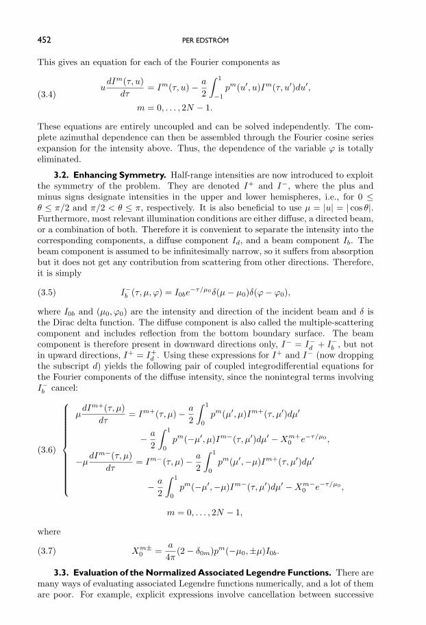
452 PER EDSTROM
This gives an equation for each of the Fourier components as
udIm(τ, u)
dτ= Im(τ, u) − a
2
∫ 1
−1pm(u′, u)Im(τ, u′)du′,
m = 0, . . . , 2N − 1.
(3.4)
These equations are entirely uncoupled and can be solved independently. The com-plete azimuthal dependence can then be assembled through the Fourier cosine seriesexpansion for the intensity above. Thus, the dependence of the variable ϕ is totallyeliminated.
3.2. Enhancing Symmetry. Half-range intensities are now introduced to exploitthe symmetry of the problem. They are denoted I+ and I−, where the plus andminus signs designate intensities in the upper and lower hemispheres, i.e., for 0 ≤θ ≤ π/2 and π/2 < θ ≤ π, respectively. It is also beneficial to use μ = |u| = | cos θ|.Furthermore, most relevant illumination conditions are either diffuse, a directed beam,or a combination of both. Therefore it is convenient to separate the intensity into thecorresponding components, a diffuse component Id, and a beam component Ib. Thebeam component is assumed to be infinitesimally narrow, so it suffers from absorptionbut it does not get any contribution from scattering from other directions. Therefore,it is simply
(3.5) I−b (τ, μ, ϕ) = I0be
−τ/μ0δ(μ − μ0)δ(ϕ − ϕ0),
where I0b and (μ0, ϕ0) are the intensity and direction of the incident beam and δ isthe Dirac delta function. The diffuse component is also called the multiple-scatteringcomponent and includes reflection from the bottom boundary surface. The beamcomponent is therefore present in downward directions only, I− = I−
d + I−b , but not
in upward directions, I+ = I+d . Using these expressions for I+ and I− (now dropping
the subscript d) yields the following pair of coupled integrodifferential equations forthe Fourier components of the diffuse intensity, since the nonintegral terms involvingI−b cancel:⎧⎪⎪⎪⎪⎪⎪⎪⎪⎪⎪⎪⎨⎪⎪⎪⎪⎪⎪⎪⎪⎪⎪⎪⎩
μdIm+(τ, μ)
dτ= Im+(τ, μ) − a
2
∫ 1
0pm(μ′, μ)Im+(τ, μ′)dμ′
− a
2
∫ 1
0pm(−μ′, μ)Im−(τ, μ′)dμ′ − Xm+
0 e−τ/μ0 ,
−μdIm−(τ, μ)
dτ= Im−(τ, μ) − a
2
∫ 1
0pm(μ′,−μ)Im+(τ, μ′)dμ′
− a
2
∫ 1
0pm(−μ′,−μ)Im−(τ, μ′)dμ′ − Xm−
0 e−τ/μ0 ,
(3.6)
m = 0, . . . , 2N − 1,
where
(3.7) Xm±0 =
a
4π(2 − δ0m)pm(−μ0,±μ)I0b.
3.3. Evaluation of the Normalized Associated Legendre Functions. There aremany ways of evaluating associated Legendre functions numerically, and a lot of themare poor. For example, explicit expressions involve cancellation between successive
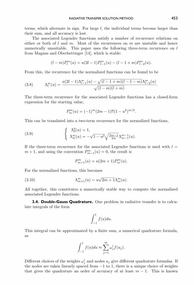
RADIATIVE TRANSFER SOLUTION METHOD 453
terms, which alternate in sign. For large l, the individual terms become larger thantheir sum, and all accuracy is lost.
The associated Legendre functions satisfy a number of recurrence relations oneither or both of l and m. Most of the recurrences on m are unstable and hencenumerically unsuitable. This paper uses the following three-term recurrence on lfrom Magnus and Oberhettinger [14], which is stable:
(l − m)Pml (u) = u(2l − 1)Pm
l−1(u) − (l − 1 + m)Pml−2(u).
From this, the recurrence for the normalized functions can be found to be
(3.8) Λml (u) =
u(2l − 1)Λml−1(u) − √
(l − 1 + m)(l − 1 − m)Λml−2(u)√
(l − m)(l + m).
The three-term recurrence for the associated Legendre functions has a closed-formexpression for the starting value,
Pmm (u) = (−1)m(2m − 1)!!(1 − u2)m/2.
This can be translated into a two-term recurrence for the normalized functions,
(3.9)
{Λ0
0(u) = 1,
Λmm(u) = −√
1 − u2√
2m−12m Λm−1
m−1(u).
If the three-term recurrence for the associated Legendre functions is used with l =m + 1, and using the convention Pm
m−1(u) = 0, the result is
Pmm+1(u) = u(2m + 1)Pm
m (u).
For the normalized functions, this becomes
(3.10) Λmm+1(u) = u
√2m + 1Λm
m(u).
All together, this constitutes a numerically stable way to compute the normalizedassociated Legendre functions.
3.4. Double-Gauss Quadrature. One problem in radiative transfer is to calcu-late integrals of the form ∫ 1
−1f(u)du.
This integral can be approximated by a finite sum, a numerical quadrature formula,as ∫ 1
−1f(u)du ≈
m∑j=1
ω′jf(uj).
Different choices of the weights ω′j and nodes uj give different quadrature formulas. If
the nodes are taken linearly spaced from −1 to 1, there is a unique choice of weightsthat gives the quadrature an order of accuracy of at least m − 1. This is known
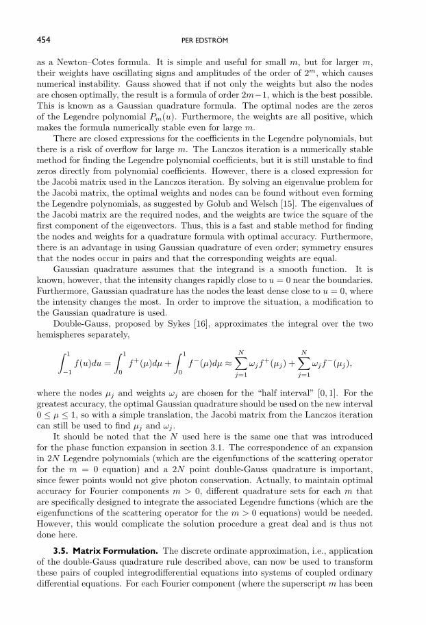
454 PER EDSTROM
as a Newton–Cotes formula. It is simple and useful for small m, but for larger m,their weights have oscillating signs and amplitudes of the order of 2m, which causesnumerical instability. Gauss showed that if not only the weights but also the nodesare chosen optimally, the result is a formula of order 2m−1, which is the best possible.This is known as a Gaussian quadrature formula. The optimal nodes are the zerosof the Legendre polynomial Pm(u). Furthermore, the weights are all positive, whichmakes the formula numerically stable even for large m.
There are closed expressions for the coefficients in the Legendre polynomials, butthere is a risk of overflow for large m. The Lanczos iteration is a numerically stablemethod for finding the Legendre polynomial coefficients, but it is still unstable to findzeros directly from polynomial coefficients. However, there is a closed expression forthe Jacobi matrix used in the Lanczos iteration. By solving an eigenvalue problem forthe Jacobi matrix, the optimal weights and nodes can be found without even formingthe Legendre polynomials, as suggested by Golub and Welsch [15]. The eigenvalues ofthe Jacobi matrix are the required nodes, and the weights are twice the square of thefirst component of the eigenvectors. Thus, this is a fast and stable method for findingthe nodes and weights for a quadrature formula with optimal accuracy. Furthermore,there is an advantage in using Gaussian quadrature of even order; symmetry ensuresthat the nodes occur in pairs and that the corresponding weights are equal.
Gaussian quadrature assumes that the integrand is a smooth function. It isknown, however, that the intensity changes rapidly close to u = 0 near the boundaries.Furthermore, Gaussian quadrature has the nodes the least dense close to u = 0, wherethe intensity changes the most. In order to improve the situation, a modification tothe Gaussian quadrature is used.
Double-Gauss, proposed by Sykes [16], approximates the integral over the twohemispheres separately,∫ 1
−1f(u)du =
∫ 1
0f+(μ)dμ +
∫ 1
0f−(μ)dμ ≈
N∑j=1
ωjf+(μj) +
N∑j=1
ωjf−(μj),
where the nodes μj and weights ωj are chosen for the “half interval” [0, 1]. For thegreatest accuracy, the optimal Gaussian quadrature should be used on the new interval0 ≤ μ ≤ 1, so with a simple translation, the Jacobi matrix from the Lanczos iterationcan still be used to find μj and ωj .
It should be noted that the N used here is the same one that was introducedfor the phase function expansion in section 3.1. The correspondence of an expansionin 2N Legendre polynomials (which are the eigenfunctions of the scattering operatorfor the m = 0 equation) and a 2N point double-Gauss quadrature is important,since fewer points would not give photon conservation. Actually, to maintain optimalaccuracy for Fourier components m > 0, different quadrature sets for each m thatare specifically designed to integrate the associated Legendre functions (which are theeigenfunctions of the scattering operator for the m > 0 equations) would be needed.However, this would complicate the solution procedure a great deal and is thus notdone here.
3.5. Matrix Formulation. The discrete ordinate approximation, i.e., applicationof the double-Gauss quadrature rule described above, can now be used to transformthese pairs of coupled integrodifferential equations into systems of coupled ordinarydifferential equations. For each Fourier component (where the superscript m has been
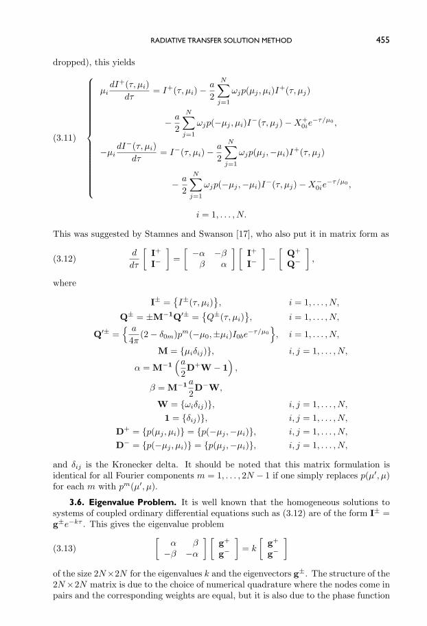
RADIATIVE TRANSFER SOLUTION METHOD 455
dropped), this yields⎧⎪⎪⎪⎪⎪⎪⎪⎪⎪⎪⎪⎪⎪⎪⎪⎪⎨⎪⎪⎪⎪⎪⎪⎪⎪⎪⎪⎪⎪⎪⎪⎪⎪⎩
μidI+(τ, μi)
dτ= I+(τ, μi) − a
2
N∑j=1
ωjp(μj , μi)I+(τ, μj)
− a
2
N∑j=1
ωjp(−μj , μi)I−(τ, μj) − X+0ie
−τ/μ0 ,
−μidI−(τ, μi)
dτ= I−(τ, μi) − a
2
N∑j=1
ωjp(μj ,−μi)I+(τ, μj)
− a
2
N∑j=1
ωjp(−μj ,−μi)I−(τ, μj) − X−0ie
−τ/μ0 ,
(3.11)
i = 1, . . . , N.
This was suggested by Stamnes and Swanson [17], who also put it in matrix form as
(3.12)d
dτ
[I+
I−
]=
[ −α −ββ α
] [I+
I−
]−
[Q+
Q−
],
where
I± ={I±(τ, μi)
}, i = 1, . . . , N,
Q± = ±M−1Q′± ={Q±(τ, μi)
}, i = 1, . . . , N,
Q′± ={ a
4π(2 − δ0m)pm(−μ0,±μi)I0be
−τ/μ0
}, i = 1, . . . , N,
M = {μiδij)}, i, j = 1, . . . , N,
α = M−1(a
2D+W − 1
),
β = M−1 a
2D−W,
W = {ωiδij)}, i, j = 1, . . . , N,
1 = {δij)}, i, j = 1, . . . , N,
D+ = {p(μj , μi)} = {p(−μj ,−μi)}, i, j = 1, . . . , N,
D− = {p(−μj , μi)} = {p(μj ,−μi)}, i, j = 1, . . . , N,
and δij is the Kronecker delta. It should be noted that this matrix formulation isidentical for all Fourier components m = 1, . . . , 2N − 1 if one simply replaces p(μ′, μ)for each m with pm(μ′, μ).
3.6. Eigenvalue Problem. It is well known that the homogeneous solutions tosystems of coupled ordinary differential equations such as (3.12) are of the form I± =g±e−kτ . This gives the eigenvalue problem
(3.13)[
α β−β −α
] [g+
g−
]= k
[g+
g−
]of the size 2N×2N for the eigenvalues k and the eigenvectors g±. The structure of the2N ×2N matrix is due to the choice of numerical quadrature where the nodes come inpairs and the corresponding weights are equal, but it is also due to the phase function
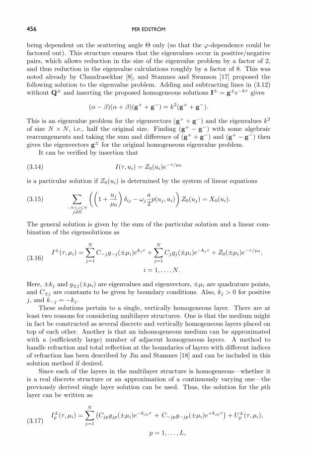
456 PER EDSTROM
being dependent on the scattering angle Θ only (so that the ϕ-dependence could befactored out). This structure ensures that the eigenvalues occur in positive/negativepairs, which allows reduction in the size of the eigenvalue problem by a factor of 2,and thus reduction in the eigenvalue calculations roughly by a factor of 8. This wasnoted already by Chandrasekhar [8], and Stamnes and Swanson [17] proposed thefollowing solution to the eigenvalue problem. Adding and subtracting lines in (3.12)without Q± and inserting the proposed homogeneous solutions I± = g±e−kτ gives
(α − β)(α + β)(g+ + g−) = k2(g+ + g−).
This is an eigenvalue problem for the eigenvectors (g+ + g−) and the eigenvalues k2
of size N × N , i.e., half the original size. Finding (g+ − g−) with some algebraicrearrangements and taking the sum and difference of (g+ + g−) and (g+ − g−) thengives the eigenvectors g± for the original homogeneous eigenvalue problem.
It can be verified by insertion that
(3.14) I(τ, ui) = Z0(ui)e−τ/μ0
is a particular solution if Z0(ui) is determined by the system of linear equations
(3.15)∑
−N≤j≤N
j �=0
((1 +
uj
μ0
)δij − ωj
a
2p(uj , ui)
)Z0(uj) = X0(ui).
The general solution is given by the sum of the particular solution and a linear com-bination of the eigensolutions as
I±(τ, μi) =N∑
j=1
C−jg−j(±μi)ekjτ +N∑
j=1
Cjgj(±μi)e−kjτ + Z0(±μi)e−τ/μ0 ,
i = 1, . . . , N.
(3.16)
Here, ±kj and g±j(±μi) are eigenvalues and eigenvectors, ±μi are quadrature points,and C±j are constants to be given by boundary conditions. Also, kj > 0 for positivej, and k−j = −kj .
These solutions pertain to a single, vertically homogeneous layer. There are atleast two reasons for considering multilayer structures. One is that the medium mightin fact be constructed as several discrete and vertically homogeneous layers placed ontop of each other. Another is that an inhomogeneous medium can be approximatedwith a (sufficiently large) number of adjacent homogeneous layers. A method tohandle refraction and total reflection at the boundaries of layers with different indicesof refraction has been described by Jin and Stamnes [18] and can be included in thissolution method if desired.
Since each of the layers in the multilayer structure is homogeneous—whether itis a real discrete structure or an approximation of a continuously varying one—thepreviously derived single layer solution can be used. Thus, the solution for the pthlayer can be written as
I±p (τ, μi) =
N∑j=1
(Cjpgjp(±μi)e−kjpτ + C−jpg−jp(±μi)e+kjpτ
)+ U±
p (τ, μi),
p = 1, . . . , L,
(3.17)
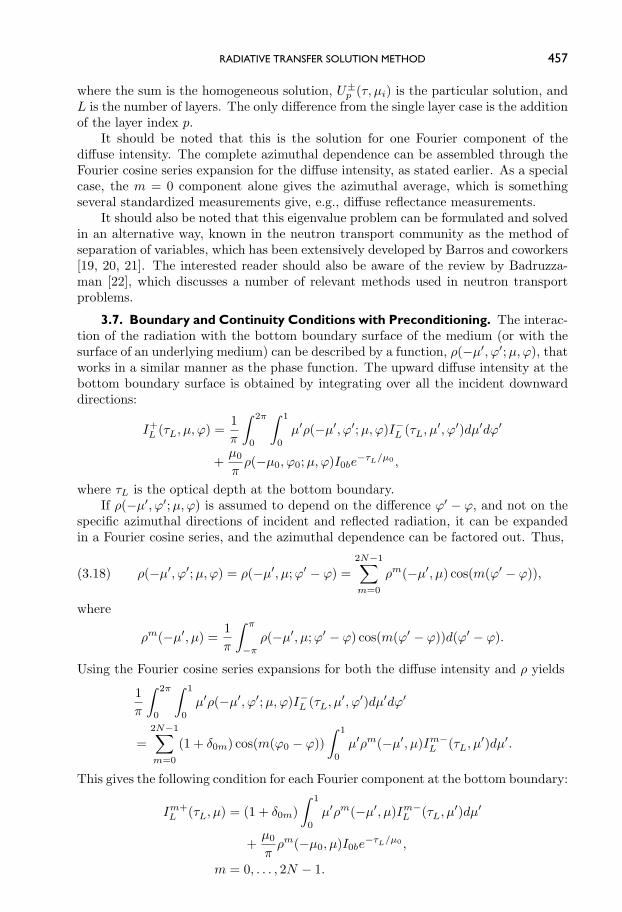
RADIATIVE TRANSFER SOLUTION METHOD 457
where the sum is the homogeneous solution, U±p (τ, μi) is the particular solution, and
L is the number of layers. The only difference from the single layer case is the additionof the layer index p.
It should be noted that this is the solution for one Fourier component of thediffuse intensity. The complete azimuthal dependence can be assembled through theFourier cosine series expansion for the diffuse intensity, as stated earlier. As a specialcase, the m = 0 component alone gives the azimuthal average, which is somethingseveral standardized measurements give, e.g., diffuse reflectance measurements.
It should also be noted that this eigenvalue problem can be formulated and solvedin an alternative way, known in the neutron transport community as the method ofseparation of variables, which has been extensively developed by Barros and coworkers[19, 20, 21]. The interested reader should also be aware of the review by Badruzza-man [22], which discusses a number of relevant methods used in neutron transportproblems.
3.7. Boundary and Continuity Conditions with Preconditioning. The interac-tion of the radiation with the bottom boundary surface of the medium (or with thesurface of an underlying medium) can be described by a function, ρ(−μ′, ϕ′;μ, ϕ), thatworks in a similar manner as the phase function. The upward diffuse intensity at thebottom boundary surface is obtained by integrating over all the incident downwarddirections:
I+L (τL, μ, ϕ) =
1π
∫ 2π
0
∫ 1
0μ′ρ(−μ′, ϕ′;μ, ϕ)I−
L (τL, μ′, ϕ′)dμ′dϕ′
+μ0
πρ(−μ0, ϕ0;μ, ϕ)I0be
−τL/μ0 ,
where τL is the optical depth at the bottom boundary.If ρ(−μ′, ϕ′;μ, ϕ) is assumed to depend on the difference ϕ′ − ϕ, and not on the
specific azimuthal directions of incident and reflected radiation, it can be expandedin a Fourier cosine series, and the azimuthal dependence can be factored out. Thus,
(3.18) ρ(−μ′, ϕ′;μ, ϕ) = ρ(−μ′, μ;ϕ′ − ϕ) =2N−1∑m=0
ρm(−μ′, μ) cos(m(ϕ′ − ϕ)),
where
ρm(−μ′, μ) =1π
∫ π
−π
ρ(−μ′, μ;ϕ′ − ϕ) cos(m(ϕ′ − ϕ))d(ϕ′ − ϕ).
Using the Fourier cosine series expansions for both the diffuse intensity and ρ yields
1π
∫ 2π
0
∫ 1
0μ′ρ(−μ′, ϕ′;μ, ϕ)I−
L (τL, μ′, ϕ′)dμ′dϕ′
=2N−1∑m=0
(1 + δ0m) cos(m(ϕ0 − ϕ))∫ 1
0μ′ρm(−μ′, μ)Im−
L (τL, μ′)dμ′.
This gives the following condition for each Fourier component at the bottom boundary:
Im+L (τL, μ) = (1 + δ0m)
∫ 1
0μ′ρm(−μ′, μ)Im−
L (τL, μ′)dμ′
+μ0
πρm(−μ0, μ)I0be
−τL/μ0 ,
m = 0, . . . , 2N − 1.
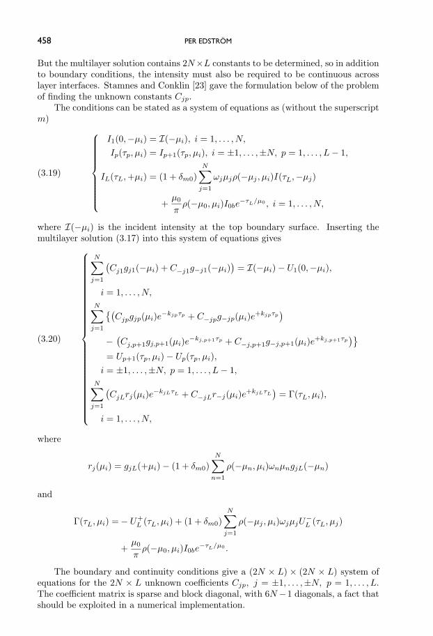
458 PER EDSTROM
But the multilayer solution contains 2N ×L constants to be determined, so in additionto boundary conditions, the intensity must also be required to be continuous acrosslayer interfaces. Stamnes and Conklin [23] gave the formulation below of the problemof finding the unknown constants Cjp.
The conditions can be stated as a system of equations as (without the superscriptm)
(3.19)
⎧⎪⎪⎪⎪⎪⎪⎪⎪⎨⎪⎪⎪⎪⎪⎪⎪⎪⎩
I1(0,−μi) = I(−μi), i = 1, . . . , N,
Ip(τp, μi) = Ip+1(τp, μi), i = ±1, . . . ,±N, p = 1, . . . , L − 1,
IL(τL,+μi) = (1 + δm0)N∑
j=1
ωjμjρ(−μj , μi)I(τL,−μj)
+μ0
πρ(−μ0, μi)I0be
−τL/μ0 , i = 1, . . . , N,
where I(−μi) is the incident intensity at the top boundary surface. Inserting themultilayer solution (3.17) into this system of equations gives
(3.20)
⎧⎪⎪⎪⎪⎪⎪⎪⎪⎪⎪⎪⎪⎪⎪⎪⎪⎪⎪⎪⎪⎪⎪⎪⎪⎪⎨⎪⎪⎪⎪⎪⎪⎪⎪⎪⎪⎪⎪⎪⎪⎪⎪⎪⎪⎪⎪⎪⎪⎪⎪⎪⎩
N∑j=1
(Cj1gj1(−μi) + C−j1g−j1(−μi)
)= I(−μi) − U1(0,−μi),
i = 1, . . . , N,
N∑j=1
{(Cjpgjp(μi)e−kjpτp + C−jpg−jp(μi)e+kjpτp
)− (
Cj,p+1gj,p+1(μi)e−kj,p+1τp + C−j,p+1g−j,p+1(μi)e+kj,p+1τp)}
= Up+1(τp, μi) − Up(τp, μi),i = ±1, . . . ,±N, p = 1, . . . , L − 1,
N∑j=1
(CjLrj(μi)e−kjLτL + C−jLr−j(μi)e+kjLτL
)= Γ(τL, μi),
i = 1, . . . , N,
where
rj(μi) = gjL(+μi) − (1 + δm0)N∑
n=1
ρ(−μn, μi)ωnμngjL(−μn)
and
Γ(τL, μi) = − U+L (τL, μi) + (1 + δm0)
N∑j=1
ρ(−μj , μi)ωjμjU−L (τL, μj)
+μ0
πρ(−μ0, μi)I0be
−τL/μ0 .
The boundary and continuity conditions give a (2N × L) × (2N × L) system ofequations for the 2N × L unknown coefficients Cjp, j = ±1, . . . ,±N, p = 1, . . . , L.The coefficient matrix is sparse and block diagonal, with 6N −1 diagonals, a fact thatshould be exploited in a numerical implementation.
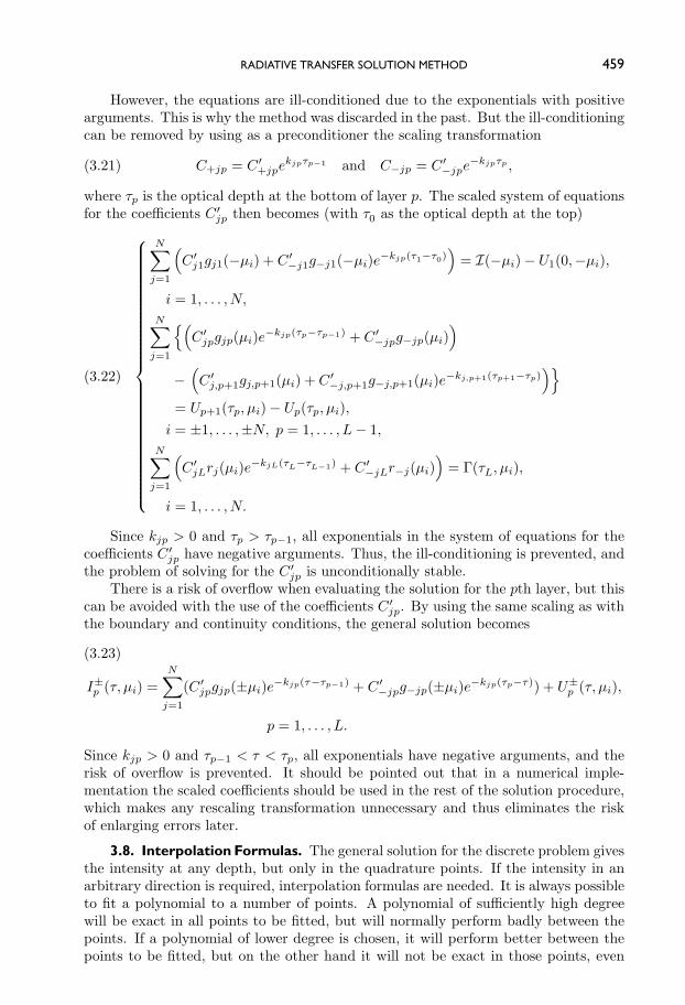
RADIATIVE TRANSFER SOLUTION METHOD 459
However, the equations are ill-conditioned due to the exponentials with positivearguments. This is why the method was discarded in the past. But the ill-conditioningcan be removed by using as a preconditioner the scaling transformation
(3.21) C+jp = C ′+jpe
kjpτp−1 and C−jp = C ′−jpe
−kjpτp ,
where τp is the optical depth at the bottom of layer p. The scaled system of equationsfor the coefficients C ′
jp then becomes (with τ0 as the optical depth at the top)
(3.22)
⎧⎪⎪⎪⎪⎪⎪⎪⎪⎪⎪⎪⎪⎪⎪⎪⎪⎪⎪⎪⎪⎪⎪⎪⎪⎪⎨⎪⎪⎪⎪⎪⎪⎪⎪⎪⎪⎪⎪⎪⎪⎪⎪⎪⎪⎪⎪⎪⎪⎪⎪⎪⎩
N∑j=1
(C ′
j1gj1(−μi) + C ′−j1g−j1(−μi)e−kjp(τ1−τ0)
)= I(−μi) − U1(0,−μi),
i = 1, . . . , N,
N∑j=1
{(C ′
jpgjp(μi)e−kjp(τp−τp−1) + C ′−jpg−jp(μi)
)−
(C ′
j,p+1gj,p+1(μi) + C ′−j,p+1g−j,p+1(μi)e−kj,p+1(τp+1−τp)
)}= Up+1(τp, μi) − Up(τp, μi),
i = ±1, . . . ,±N, p = 1, . . . , L − 1,
N∑j=1
(C ′
jLrj(μi)e−kjL(τL−τL−1) + C ′−jLr−j(μi)
)= Γ(τL, μi),
i = 1, . . . , N.
Since kjp > 0 and τp > τp−1, all exponentials in the system of equations for thecoefficients C ′
jp have negative arguments. Thus, the ill-conditioning is prevented, andthe problem of solving for the C ′
jp is unconditionally stable.There is a risk of overflow when evaluating the solution for the pth layer, but this
can be avoided with the use of the coefficients C ′jp. By using the same scaling as with
the boundary and continuity conditions, the general solution becomes
I±p (τ, μi) =
N∑j=1
(C ′jpgjp(±μi)e−kjp(τ−τp−1) + C ′
−jpg−jp(±μi)e−kjp(τp−τ)) + U±p (τ, μi),
p = 1, . . . , L.
(3.23)
Since kjp > 0 and τp−1 < τ < τp, all exponentials have negative arguments, and therisk of overflow is prevented. It should be pointed out that in a numerical imple-mentation the scaled coefficients should be used in the rest of the solution procedure,which makes any rescaling transformation unnecessary and thus eliminates the riskof enlarging errors later.
3.8. Interpolation Formulas. The general solution for the discrete problem givesthe intensity at any depth, but only in the quadrature points. If the intensity in anarbitrary direction is required, interpolation formulas are needed. It is always possibleto fit a polynomial to a number of points. A polynomial of sufficiently high degreewill be exact in all points to be fitted, but will normally perform badly between thepoints. If a polynomial of lower degree is chosen, it will perform better between thepoints to be fitted, but on the other hand it will not be exact in those points, even
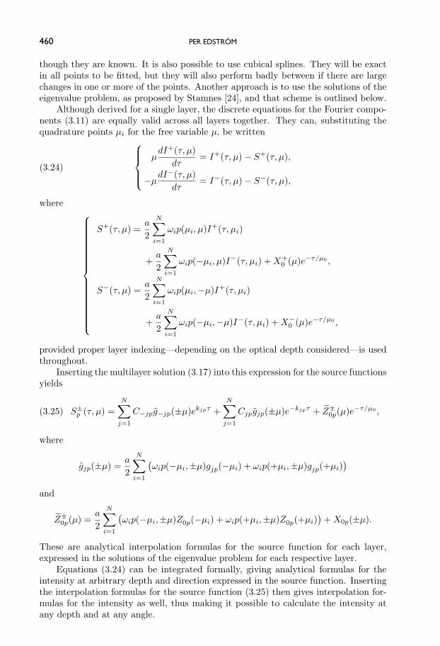
460 PER EDSTROM
though they are known. It is also possible to use cubical splines. They will be exactin all points to be fitted, but they will also perform badly between if there are largechanges in one or more of the points. Another approach is to use the solutions of theeigenvalue problem, as proposed by Stamnes [24], and that scheme is outlined below.
Although derived for a single layer, the discrete equations for the Fourier compo-nents (3.11) are equally valid across all layers together. They can, substituting thequadrature points μi for the free variable μ, be written
(3.24)
⎧⎪⎪⎨⎪⎪⎩μ
dI+(τ, μ)dτ
= I+(τ, μ) − S+(τ, μ),
−μdI−(τ, μ)
dτ= I−(τ, μ) − S−(τ, μ),
where ⎧⎪⎪⎪⎪⎪⎪⎪⎪⎪⎪⎪⎪⎪⎪⎪⎨⎪⎪⎪⎪⎪⎪⎪⎪⎪⎪⎪⎪⎪⎪⎪⎩
S+(τ, μ) =a
2
N∑i=1
ωip(μi, μ)I+(τ, μi)
+a
2
N∑i=1
ωip(−μi, μ)I−(τ, μi) + X+0 (μ)e−τ/μ0 ,
S−(τ, μ) =a
2
N∑i=1
ωip(μi,−μ)I+(τ, μi)
+a
2
N∑i=1
ωip(−μi,−μ)I−(τ, μi) + X−0 (μ)e−τ/μ0 ,
provided proper layer indexing—depending on the optical depth considered—is usedthroughout.
Inserting the multilayer solution (3.17) into this expression for the source functionsyields
(3.25) S±p (τ, μ) =
N∑j=1
C−jpg−jp(±μ)ekjpτ +N∑
j=1
Cjpgjp(±μ)e−kjpτ + Z±0p(μ)e−τ/μ0 ,
where
gjp(±μ) =a
2
N∑i=1
(ωip(−μi,±μ)gjp(−μi) + ωip(+μi,±μ)gjp(+μi)
)and
Z±0p(μ) =
a
2
N∑i=1
(ωip(−μi,±μ)Z0p(−μi) + ωip(+μi,±μ)Z0p(+μi)
)+ X0p(±μ).
These are analytical interpolation formulas for the source function for each layer,expressed in the solutions of the eigenvalue problem for each respective layer.
Equations (3.24) can be integrated formally, giving analytical formulas for theintensity at arbitrary depth and direction expressed in the source function. Insertingthe interpolation formulas for the source function (3.25) then gives interpolation for-mulas for the intensity as well, thus making it possible to calculate the intensity atany depth and at any angle.
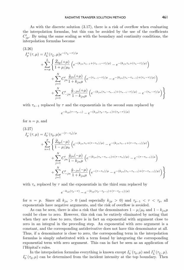
RADIATIVE TRANSFER SOLUTION METHOD 461
As with the discrete solution (3.17), there is a risk of overflow when evaluatingthe interpolation formulas, but this can be avoided by the use of the coefficientsC ′
jp. By using the same scaling as with the boundary and continuity conditions, theinterpolation formulas become
I+p (τ, μ) = I+
L (τL, μ)e−(τL−τ)/μ
+L∑
n=p
{Z0p(+μ)1 + μ/μ0
(e−(kjnτn−1+(τn−1−τ)/μ) − e−(kjnτn+(τn−τ)/μ)
)
+N∑
j=1
C ′jn
gjn(+μ)1 + kjnμ
(e−(τn−1−τ)/μ − e−(kjn(τn−τn−1)+(τn−τ)/μ)
)
+N∑
j=1
C ′−jn
g−jn(+μ)1 − kjnμ
(e−(kjn(τn−τn−1)+(τn−1−τ)/μ) − e−(τn−τ)/μ
)}
(3.26)
with τn−1 replaced by τ and the exponentials in the second sum replaced by
e−kjp(τ−τp−1) − e−(kjp(τp−τp−1)+(τp−τ)/μ)
for n = p, and
I−p (τ, μ) = I−
0 (τ0, μ)e−(τ−τ0)/μ
+p∑
n=1
{Z0p(−μ)1 − μ/μ0
(e−(kjnτn+(τ−τn)/μ) − e−(kjnτn−1+(τ−τn−1)/μ)
)
+N∑
j=1
C ′jn
gjn(−μ)1 − kjnμ
(e−(kjn(τn−τn−1)+(τ−τn)/μ) − e−(τ−τn−1)/μ
)
+N∑
j=1
C ′−jn
g−jn(−μ)1 + kjnμ
(e−(τ−τn)/μ − e−(kjn(τn−τn−1)+(τ−τn−1)/μ)
)}
(3.27)
with τn replaced by τ and the exponentials in the third sum replaced by
e−kjp(τp−τ) − e−(kjp(τp−τp−1)+(τ−τp−1)/μ)
for n = p. Since all kjn > 0 (and especially kjp > 0) and τp−1 < τ < τp, allexponentials have negative arguments, and the risk of overflow is avoided.
As can be seen, there is also a risk that the denominators 1 − μ/μ0 and 1 − kjnμcould be close to zero. However, this risk can be entirely eliminated by noting thatwhen they are close to zero, there is in fact an exponential with argument close tozero in an integral in the preceding step. An exponential with zero argument is aconstant, and the corresponding antiderivative does not have this denominator at all.Thus, if a denominator is close to zero, the corresponding term in the interpolationformulas is simply substituted with a term found by integrating the correspondingexponential term with zero argument. This can in fact be seen as an application ofl’Hopital’s rules.
In the interpolation formulas everything is known except I−0 (τ0, μ) and I+
L (τL, μ).I−0 (τ0, μ) can be determined from the incident intensity at the top boundary. Then
462 PER EDSTROM
I−L (τL, μ) is calculated from the interpolation formulas, and using the boundary condi-
tions I+L (τL, μ) can be found. The interpolation formulas for the intensity give exactly
the same result at the quadrature points as the discrete solution (3.17). They alsosatisfy the boundary conditions for all μ, albeit such conditions were imposed through(3.19) only at the quadrature points.
3.9. The δ-N Method. If the scattering is strongly forward-peaked, an accurateexpansion of the phase function needs a large number, up to several hundreds orthousands, of terms. To maintain accuracy throughout the solution, a comparablenumber of terms are needed in the numerical quadrature used to approximate theintegrals. This quickly gives very large eigenvalue problems and systems of equations,and since the computation time for these grows approximately as the third powerof the size, the problem soon becomes intractable. The memory requirements alsoincrease rapidly. To avoid this, a transformation proposed by Wiscombe [25], the δ-Nmethod, can be applied to give a problem with a less peaked phase function.
The idea is to consider the beams scattered through the small angles within thesharp forward peak as unscattered, and truncate this peak from the phase function.The phase function is separated into the sum of a Dirac delta function in the forwarddirection and a truncated phase function, which is expanded in a series of Legendrepolynomials with a much smaller number of terms, preferably equal to the number ofquadrature points, i.e., 2N .
On one hand, the phase function is directly expanded in Legendre polynomials as
p(cos Θ) =Nlarge∑l=0
(2l + 1)χlPl(cosΘ).
On the other hand, the delta peak is first removed and then the remainder is expandedas
p(cos Θ) = fp′′(cos Θ) + (1 − f)p′(cos Θ)
≈ fδ(1 − cos Θ) + (1 − f)2N−1∑l=0
(2l + 1)χlPl(cos Θ)
≡ pδ-N (cos Θ),
where f is a dimensionless parameter between 0 and 1 (f thus denotes the fraction ofthe phase function that is contained in the separated delta peak). Demanding thatthe coefficients for Legendre polynomial expansion are the same for p and pδ-N , aslong as they have common terms, yields
χl = f + (1 − f)χl, or χl =χl − f
1 − f, l = 0, . . . , 2N − 1.
The expansion for pδ-N is truncated by demanding χ2N = 0, which gives f = χ2N .Replacing p with pδ-N in the equation of radiative transfer and introducing τ ′ =(1 − af)τ and a′ = 1−f
1−af a yields a structurally equivalent equation. Hence, the δ-Nmethod does not change the mathematical form of the radiative transfer equation. Itonly changes the optical properties of the medium to make it appear less anisotropic.
Thus, the δ-N method allows handling of strongly forward-peaked phase func-tions (g close to 1) with maintained accuracy without a tremendously increased com-putational burden. The δ-N method also provides maintained accuracy for all g for
RADIATIVE TRANSFER SOLUTION METHOD 463
significantly lower N than otherwise needed. However, the closer g is to zero, thesmaller N is needed anyway, so the savings in computation time diminish with de-creasing |g|. The overhead introduced by the method is insignificant compared to thecore calculations.
Morel [26] reports an alternative way of dealing with strongly forward-peakedscattering. He points out that it is not the accuracy of the truncated phase functionexpansion that matters, but rather the accuracy of the representation of the sourcefunction. Thus, if the solution is well represented by the given Legendre polynomialexpansion, an accurate solution will be obtained regardless of the convergence of thetruncated phase function expansion. Morel presents a Galerkin quadrature approach,which under this assumption treats the scattering exactly, and thus leaves the solu-tion invariant to the δ-N transformation. Unfortunately, this approach is limited tothe azimuthally averaged (m = 0) case, since the solution for Fourier componentsm > 0 cannot be well represented by Legendre polynomials, but needs the associatedLegendre functions.
3.10. Intensity Correction Procedures. The accuracy of the intensity compu-tation is generally improved by the use of the δ-N method except in the direction ofthe forward peak, but the δ-N method also introduces minor errors in other direc-tions. However, combining the δ-N method with exact computation of low orders ofscattering can considerably reduce the error. The purpose is to achieve high accuracywith small N , to speed up calculations. The TMS and IMS methods of Nakajima andTanaka [27] serve to correct for single scattering and secondary and higher orders ofscattering, respectively.
The phase function resulting from the δ-N method oscillates around the originalphase function with a magnitude depending on the parameter f . This gives thecomputed intensities an oscillating behavior, which becomes more apparent the morepeaked the phase function is. Since single scattering resembles the phase function, itwould be a good idea to compute the single scattering exactly to account for errorsdue to the δ-N method.
Exact solutions for the single-scattered intensity are easy to derive. Using theintegrodifferential equations for the Fourier components (3.6) without the multiplescattering terms, and allowing for the optical properties to vary between layers, giveselementary first-order differential equations that are readily solved.
The TMS method subtracts the erroneous single-scattered intensity obtained byusing the scaled τ ′, the scaled a′, and the phase function
p′(cosΘ) =2N−1∑l=0
(2l + 1)χlPl(cos Θ)
from the δ-N method, and adds back the exactly calculated single-scattered intensityobtained by using the scaled τ ′, a
1−af (where the denominator is a consequence of thescaled τ ′), and the exact phase function
p(cos Θ) =Nlarge∑l=0
(2l + 1)χlPl(cos Θ)
with all available terms. This can be denoted ITMS = I ′ + ΔITMS = I ′ − I ′ss + Icorr
ss ,where I ′ is the intensity computed by using the δ-N method, and I ′
ss and Icorrss are
the single-scattered intensities described above.
464 PER EDSTROM
The TMS method gives a substantial improvement for the computed intensity, andthe oscillations are suppressed. An error remains only in the direction of the forwardpeak. This is corrected in the IMS method by accounting for secondary and higherorders of scattering. Of course, exact solutions cannot be found for these corrections,since that would mean actually solving the overall problem. Instead, an exact solutioncan be derived symbolically, and then intelligent approximations need to be made inorder to make the solution possible to use in the IMS method in practice. Reachingthe final expression for the IMS method requires a substantial amount of algebra, andthe original paper is also rather brief. However, the essentials will be outlined here.
The IMS method corrects only the intensity inside a cone centered on the forwardpeak direction, and thus affects only the downward intensity. Therefore, in this sec-tion, some simplifying notation can be used. All intensity variables I implicitly meanI(τ, −μ, ϕ) and all angular integrals 1
4π
∫4π
p · Idω′ implicitly mean
14π
∫ 2π
0
∫ 1
−1p(τ, μ′, ϕ′;−μ, ϕ)I(τ, μ′, ϕ′)dμ′dϕ′.
The optical properties, a, f , and p · I0b implicitly mean, respectively, a(τ), f(τ), andp(τ, −μ0, ϕ0;−μ, ϕ)I0b.
Using the notation Itrue = ITMS − ΔIIMS , where Itrue is the solution to theexact radiative transfer equation, what is left to be found is an expression for the IMScorrection term ΔIIMS = ITMS −Itrue . Differentiating this, using the definitions of τ ′,ITMS , Itrue , and p′′ = 1
f (p − (1 − f)p′), defining the δ-N multiple-scattered intensityas I ′
mult = I ′ − I ′ss , and algebraically rearranging gives
(3.28) −μd
dτ(ΔIIMS ) = ΔIIMS − a
4π
∫4π
p · ΔIIMSdω′ − (Q1 + Q2 + Q3),
where
Q1 = af
(I ′mult − 1
4π
∫4π
p′′ · I ′multdω′
),
Q2 = af
(Icorrss − 1
4π
∫4π
p′′ · Icorrss dω′
),
and
Q3 =a
4πp · I0b
(e−τ ′/μ0 − e−τ/μ0
)− a
4π(1 − f)
∫4π
p′ · (Icorrss − I ′
ss) dω′.
This exact equation for the IMS correction term ΔIIMS is more complicated thanthe original radiative transfer equation, so several approximations need to be madein order to make the IMS method practically useful. First,
− a
4π
∫4π
p · ΔIIMSdω′ ≈ 0
and Q1 ≈ 0, since their contribution to the narrow forward peak, where the IMScorrection method is used, is negligible. Second,
Q2 ≈ I0b
4π
(af)2
1 − af
e−τ ′/μ0
μ0τ ′
(p′′ − 1
4π
∫4π
p′′ · p′′dω′)
RADIATIVE TRANSFER SOLUTION METHOD 465
and
Q3 ≈ I0b
4π
(af)2
1 − af
e−τ ′/μ0
μ0τ ′p′′,
where the reasons are more complex, so the interested reader is directed to the originalpaper by Nakajima and Tanaka [27]. Finally, the IMS method uses vertically averagedoptical properties:
a =
(p∑
n=1
anτn
)/ (p∑
n=1
τn
),
f =
(p∑
n=1
fnanτn
)/ (p∑
n=1
anτn
),
χ′l,n =
{fn, l ≤ 2N − 1,χl,n, l > 2N − 1,
χl =
(p∑
n=1
χ′l,nanτn
)/ (p∑
n=1
fnanτn
),
p′′(cos Θ) =Nlarge∑l=0
(2l + 1)χlPl(cosΘ),
μ′0 ≡ 1
1 − afμ0,
where n is the layer index.Equation (3.28) for the IMS correction term ΔIIMS then becomes a first-order
differential equation that can be solved by integrating from 0 to τ , using eτ/μ as anintegrating factor. This gives the IMS correction term, which is then expanded into aFourier cosine series to provide the final expression that is used in the IMS method.
Thus a single Fourier component becomes
(3.29) ΔImIMS =
I0b
4π
(af)2
1 − af(2 − δ0m)pm
IMS (−μ′0,−μ)
e−τ/μ
μμ′0
∫ τ
0e(1/μ−1/μ′
0)ttdt,
where
pmIMS (−μ′
0,−μ) =Nlarge∑l=m
(2l + 1)(2χl − χ2l )Λ
ml (−μ′
0)Λml (−μ).
The intensity correction procedures further enhance the handling of stronglyforward-peaked phase functions beyond the capabilities of the δ-N method. Theseprocedures also give maintained accuracy for all g for significantly lower N than oth-erwise needed. However, the closer g is to zero, the smaller N is needed anyway, soat some point the possible savings in computation time are smaller than the overheadintroduced by the correction procedures. The correction procedures should thereforenot be used in those cases. The additional time taken for the intensity correctionprocedures consists of evaluating Legendre functions Λm
l for the larger l and m thatare used.
466 PER EDSTROM
3.11. Computational Shortcuts. As shown by King [28], the azimuthal depen-dence of the intensity typically converges well before the loop over Fourier componentshas ended. Since it is the outermost loop, much is gained if it can be terminated ear-lier. It is therefore beneficial to break the azimuthal loop when a convergence criterionhas been met, for example, when the quotient of the absolute value of a Fourier com-ponent and the cumulative sum of components is smaller than a given limit. Thissaves a significant amount of computation time in the vast majority of cases.
There is an obvious computational shortcut that allows for much faster calcu-lation of variables that depend only on the azimuthally averaged intensity, which isgiven by the zeroth Fourier component. Among these variables are total reflectance,total transmittance, total absorptance, and flux. When such variables are all thatis required, the azimuthal loop is broken after the first time instead of fulfilling theprescribed 2N times, thus giving a significant reduction in computation time.
4. Implementation and Performance. The solution method described in thispaper has recently been implemented in MATLAB under the name Dort2002, andit is now being used in the paper and printing industries for light scattering simula-tions. In the current process of replacing an older generation of simulation tools inthese sectors of industry, there is a need for more accurate models. These will offermore understanding and deeper insight in the processes of light scattering in suchcomplex media as paper. The effect of the different paper constituents on light scat-tering may then be investigated theoretically as well, with higher accuracy than realmeasurements. Application areas for Dort2002 therefore include theoretical modelcomparisons, but also fine-tuning the papermaking process, designing new paper qual-ities, color management from prepress to print, and evaluation of printing techniques.Dort2002 is, however, also intended as a general tool for radiative transfer problems,and it can be obtained from the author for evaluation.
Performance and application of Dort2002 have been studied in an extensive testseries, which will be reported elsewhere. However, it may be appropriate to give ashort summary here. Tests show that the preconditioner for the system of equationscorresponding to the boundary and continuity conditions works very well, giving acondition number close to 1 in most cases, and around 30 in the worst case. Theyalso show that the problem is very ill-conditioned without the preconditioner, havinga condition number near the largest positive floating-point number for the system. Itis also shown that the reduced eigenvalue problem is very well-conditioned, giving acondition number close to 1 in all cases. Dort2002 is shown to converge when Nincreases.
Performance tests show that the steps that are taken to improve the stability andspeed of Dort2002 are very successful, together giving an unconditionally stablesolution procedure to a problem previously considered numerically intractable, andtogether decreasing computation time with a factor of 1,000–10,000 in typical casesand with a factor up to and beyond 10,000,000 in extreme cases. Application testsshow very good agreement of Dort2002 with three established models of differenttypes and implementations when applied to different sets of relevant test problems,which gives strong support for the accuracy of Dort2002.
5. Open Questions and Future Work. The TMS and IMS methods take rela-tively little time in themselves, but far more time is taken by the evaluation of thenormalized associated Legendre functions, Λm
l (u), for the larger l and m needed forthese methods. Any studies that result in faster ways of evaluation of Λm
l (u) for largel and m would be welcome.
RADIATIVE TRANSFER SOLUTION METHOD 467
One bottleneck that remains is the generation in MATLAB of the sparse matrixin the system of equations corresponding to the boundary and continuity conditions.Although the values and the indices of the nonzero elements are known, the assigningof these values to the sparse matrix is unsatisfactorily time consuming in MATLAB,to the extent that this purely administrative part of the code consumes a significantpart of the execution time. Since all computational parts of the code are alreadyso optimized, this item is the first candidate for improving the speed of the code.This problem remains, although the current implementation has been worked out incooperation with leading MATLAB experts and although the implementation, to theauthor’s knowledge, is the best that can be done in MATLAB today. Improvementsin this direction could well be considered in future versions of MATLAB.
As an upcoming research activity, the inverse problem for the model presented inthis paper will be studied. This includes the study and development of fast and nu-merically stable algorithms for parameter estimation. The parameter estimation willbe carried out to fit model simulations to angle-resolved light scattering measurementsor to desired angle-resolved light scattering patterns. This opens the possibility of in-directly measuring parameters that are hard to determine in other ways, but also toconstructing materials with designed optical properties. The starting point is knownintensities in different directions in the form of measurements or design goals, andknown boundary conditions. In the simplest case the single scattering albedo, a, andthe asymmetry factor, g, are estimated. More complicated cases are multilayer struc-tures where a and g are estimated for all layers, possibly with different values in everylayer. In addition to this, it will be necessary to deal with the problem of surfaceeffects such as gloss in real-life measurements.
Acknowledgment. The author wishes to thank two anonymous referees for theirvaluable comments on the manuscript, and especially for pointing out some explicitreferences in the neutron transport and nuclear engineering areas.
REFERENCES
[1] A. Schuster, Radiation through a foggy atmosphere, Astrophys. J., 21(1905), pp. 1–22.(Reprinted in Selected Papers on the Transfer of Radiation, D. H. Menzel, Dover, NewYork, 1966, pp. 3–24.)
[2] P. Kubelka and F. Munk, Ein Beitrag zur Optik der Farbanstriche, Z. Tech. Phys., 11a(1931), pp. 593–601.
[3] P. Kubelka, New contributions to the optics of intensely light-scattering materials. Part I, J.Opt. Soc. Amer., 38 (1948), pp. 448–457.
[4] P. Kubelka, New contributions to the optics of intensely light-scattering materials. Part II,J. Opt. Soc. Amer., 44 (1954), pp. 330–335.
[5] G. C. Wick, Uber ebene Diffusionsprobleme, Z. Phys. 120 (1943), pp. 702–718.[6] S. Chandrasekhar, On the radiative equilibrium of a stellar atmosphere, Astrophys. J., 99
(1944), pp. 180–190.[7] S. Chandrasekhar, On the radiative equilibrium of a stellar atmosphere II, Astrophys. J., 100
(1944), pp. 76–86.[8] S. Chandrasekhar, Radiative Transfer, Dover, New York, 1960.[9] P. S. Mudgett and L. W. Richards, Multiple scattering calculations for technology, Appl.
Opt., 10 (1971), pp. 1485–1502.[10] P. S. Mudgett and L. W. Richards, Multiple scattering calculations for technology II, J.
Colloid Interf. Sci., 39 (1972), pp. 551–567.[11] Lord Rayleigh, On the light from the sky, its polarization and colour, Philos. Mag., 41 (1871),
pp. 107–120, 274–279. (Reprinted in Scientific Papers by Lord Rayleigh, Vol. I: 1869–1881,No. 8, Dover, New York, 1964.)
[12] G. Mie, Beitrage zur Optik truber Medien, Speziell Kolloidaler Metallosungen, Ann. Phys., 25(1908), pp. 377–445.
468 PER EDSTROM
[13] L. G. Henyey and J. L. Greenstein, Diffuse radiation in the galaxy, Astrophys. J., 93 (1941),pp. 70–83.
[14] W. Magnus and F. Oberhettinger, Formulas and Theorems for the Functions of Mathe-matical Physics, Chelsea, New York, 1949.
[15] G. H. Golub and J. H. Welsch, Calculation of Gauss quadrature rules, Math. Comp., 23(1969), pp. 221–230.
[16] J. B. Sykes, Approximate integration of the equation of transfer, Monthly Not. Roy. Astr.Soc., 111 (1951), pp. 377–386.
[17] K. Stamnes and R. A. Swanson, A new look at the discrete ordinate method for radiativetransfer calculations in anisotropically scattering atmospheres, J. Atmos. Sci., 38 (1981),pp. 387–399.
[18] Z. Jin and K. Stamnes, Radiative transfer in nonuniformly refracting media such as theatmosphere/ocean system, Appl. Opt., 33 (1994), pp. 431–442.
[19] R. C. De Barros and E. W. Larsen, A numerical method for one-group slab-geometry discreteordinates problems with no spatial truncation error, Nucl. Sci. Eng., 104 (1990), pp. 199–208.
[20] R. C. De Barros and E. W. Larsen, A spectral nodal method for one-group x,y-geometrydiscrete ordinates problems, Nucl. Sci. Eng., 111 (1992), pp. 34–45.
[21] R. C. De Barros, F. C. da Silva, and H. A. Filho, Recent advances in spectral nodal methodsfor x,y-geometry discrete ordinates deep penetration and eigenvalue problems, Progress inNuclear Energy, 35 (1999), pp. 293–331.
[22] A. Badruzzaman, Nodal Methods in Transport Theory, Advances in Nuclear Science and Tech-nology 21, J. Lewins and M. Becker, eds., Plenum Press, New York, 1990.
[23] K. Stamnes and P. Conklin, A new multi-layer discrete ordinate approach to radiative trans-fer in vertically inhomogeneous atmospheres, J. Quant. Spectrosc. Radiat. Transfer, 31(1984), pp. 273–282.
[24] K. Stamnes, On the computation of angular distributions of radiation in planetary atmo-spheres, J. Quant. Spectrosc. Radiat. Transfer, 28 (1982), pp. 47–51.
[25] W. J. Wiscombe, The delta-M method: Rapid yet accurate radiative flux calculations forstrongly asymmetric phase functions, J. Atmos. Sci., 34 (1977), pp. 1408–1422.
[26] J. E. Morel, A hybrid collocation-Galerkin-Sn method for solving the Boltzmann transportequation, Nucl. Sci. Eng., 101 (1989), pp. 72–87.
[27] T. Nakajima and M. Tanaka, Algorithms for radiative intensity calculations in moderatelythick atmospheres using a truncation approach, J. Quant. Spectrosc. Radiat. Transfer, 40(1988), pp. 51–69.
[28] M. D. King, Number of terms required in the Fourier expansion of the reflection function foroptically thick atmospheres, J. Quant. Spectrosc. Radiat. Transfer, 30 (1983), pp. 143–161.
[29] G. H. Golub and C. F. Van Loan, Matrix Computations, 3rd ed., Johns Hopkins UniversityPress, Baltimore, MD, 1996.

II

Numerical Performance of Stability
Enhancing and Speed Increasing Steps in
Radiative Transfer Solution Methods �
Per Edstrom
Dept. of Engineering, Physics and Mathematics, Mid Sweden University,SE-87188 Harnosand, Sweden
Abstract
Methods for solving the radiative transfer problem, which is crucial for a numberof sectors of industry, involve several numerical challenges. This paper gives a sys-tematic presentation of the effect of the steps that are needed or possible to makeany discrete ordinate radiative transfer solution method numerically efficient. Thisis done through studies of the numerical performance of the stability enhancing andspeed increasing steps used in modern tools like Disort or Dort2002.
Performance tests illustrate the effect of steps that are taken to improve stabilityand speed. It is shown how the steps together give an unconditionally stable solutionprocedure to a problem previously considered numerically intractable, and how theytogether decrease the computation time compared to a naive implementation witha factor 1 000–10 000 in typical cases and with a factor up to and beyond 10 000 000in extreme cases. It is also shown that the speed increasing steps are not introducedat the cost of reduced accuracy. Further studies and developments, which can havea positive impact on computation time, are suggested.
Key words: radiative transfer, solution method, numerical performance, stability,speed, accuracy1991 MSC: 45J05, 65R20, 65Y20, 85A25
� This work was financially supported by the Swedish printing research programT2F, ‘TryckTeknisk Forskning’.
Email address: [email protected] (Per Edstrom).
Preprint submitted to Journal of Computational and Applied Mathematics10 February 2007
1 Introduction
Radiative transfer solution methods are important tools for modelling theinteraction of radiation with turbid (scattering and absorbing) media. Appli-cations range from stellar atmospheres and infrared and visible light in spaceand in the atmosphere, to optical tomography and diffusion of neutrons. Anindustrially important application is light scattering in textile, paint, pigmentfilms, paper and print, and accurate calculation methods are crucial for thesesectors of industry.
Discrete ordinate solution methods for radiative transfer problems have beenstudied throughout the last century. In the beginning most radiative transferproblems were considered intractable because of numerical difficulties. There-fore coarse approximations were used, and methods developed slowly due tothe lack of mathematical tools. The first approximate solution to the radia-tive transfer problem was presented by Schuster [16], and Wick [26] gave thefirst general treatment of discrete ordinate methods. Chandrasekhar describeda method using spherical harmonics [2], but having read Wick’s article, headopted the discrete ordinate method, and further refined it [3]. Later, hewrote a classic exposition on radiative transfer theory in book form [4], andsince then the area has expanded tremendously. Mudgett and Richards [13,14]described a discrete ordinate method for use in technology, and reported onnumerical difficulties, as have many before and after them.
Through a great effort, ranging over several years, Stamnes and coworkers[23,21] presented in a series of papers the successive development of a sta-ble discrete ordinate algorithm, and provided a software package, Disort.Thomas and Stamnes [25] also wrote a textbook on radiative transfer in theatmosphere. In a recent paper, Edstrom [7] presented a systematic review ofthe stability enhancing and speed increasing steps used in modern discreteordinate radiative transfer algorithms. Edstrom also presented the solutionmethod Dort2002, which is adapted to light scattering simulations in paperand print, but which is also designed for methodical numerical experimentsthrough its modularized design and ability to give any kind of intermediateresults and performance data.
The point of this paper is to give a systematic presentation of the effect ofthe steps that are needed or possible to make any discrete ordinate radiativetransfer solution method numerically efficient, and in particular the effect ofthe most important steps used in modern tools like Disort or Dort2002. Tothe author’s knowledge, this has not been summarized in one single publicationbefore, in particular not with the focus on quantifying the effect of the steps.
First, a short overview of a generic solution method is given. Then the resulting
2
improvements, quantified in terms of reduced condition number and increasedspeed compared to a naive implementation, are illustrated. The speed increas-ing steps are also analyzed to verify that speed is not introduced at the costof reduced accuracy. Finally, some studies and developments that can have apositive impact on computation time are suggested.
2 Solution Method Overview
This section gives a short introduction to the radiative transfer problem, andthe structure of a modern generic discrete ordinate solution method.
Edstrom [7] states the equation of radiative transfer as
udI(τ, u, ϕ)
dτ= I(τ, u, ϕ) − a
4π
∫ 2π
0
∫ 1
−1p(u′, ϕ′; u, ϕ)I(τ, u′, ϕ′)du′dϕ′. (1)
The unknown intensity, I, at optical depth τ is considered as non-interactingbeams of radiation in all directions. The phase function, p, specifies the prob-ability distribution of scattering from incident direction (u′, ϕ′) to direction(u, ϕ), where u is cosine of polar angle, and ϕ is azimuthal angle. The shapeof the phase function may be controlled by a parameter called the asymme-try factor, g, ranging from complete forward scattering (g = 1) over isotropicscattering (g = 0) to complete backward scattering (g = −1), or it may bedefined by any number of discrete phase space moments. The single scatteringalbedo, a, is the probability for scattering given an extinction event, and isdefined as a = σs/(σa + σs), where σs and σa are the scattering and absorp-tion coefficients of the medium. The first term on the right hand side in theradiative transfer equation (1) thus gives intensity absorbed when traversinga thickness dτ , while the integral term gives the intensity scattered from allincoming directions at a point to a specified direction.
The common procedure in discrete ordinate methods is to use Fourier analysison the azimuthal angle to turn the integro-differential equation (1) into a num-ber of uncoupled equations, one for each Fourier component of the unknownintensity, which are then discretized using numerical quadrature. This yields asystem of first order linear differential equations for each layer in each Fouriercomponent. This system can be put into block matrix form (see Edstrom [7]for details) as
d
dτ
⎡⎢⎣ I+
I−
⎤⎥⎦ =
⎡⎢⎣−α −β
β α
⎤⎥⎦
⎡⎢⎣ I+
I−
⎤⎥⎦ −
⎡⎢⎣ Q+
Q−
⎤⎥⎦ , (2)
where I± = {I±(τ, μi)}, and where Q± pertains to the particular solution.The block matrices α and β are given as the solutions to Mα = a
2D+W − 1
3
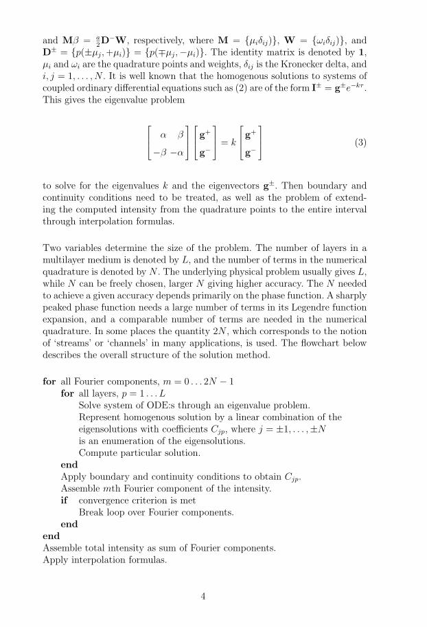
and Mβ = a2D
−W, respectively, where M = {μiδij)}, W = {ωiδij)}, andD± = {p(±μj, +μi)} = {p(∓μj,−μi)}. The identity matrix is denoted by 1,μi and ωi are the quadrature points and weights, δij is the Kronecker delta, andi, j = 1, . . . , N . It is well known that the homogenous solutions to systems ofcoupled ordinary differential equations such as (2) are of the form I± = g±e−kτ .This gives the eigenvalue problem
⎡⎢⎣ α β
−β −α
⎤⎥⎦
⎡⎢⎣ g+
g−
⎤⎥⎦ = k
⎡⎢⎣ g+
g−
⎤⎥⎦ (3)
to solve for the eigenvalues k and the eigenvectors g±. Then boundary andcontinuity conditions need to be treated, as well as the problem of extend-ing the computed intensity from the quadrature points to the entire intervalthrough interpolation formulas.
Two variables determine the size of the problem. The number of layers in amultilayer medium is denoted by L, and the number of terms in the numericalquadrature is denoted by N . The underlying physical problem usually gives L,while N can be freely chosen, larger N giving higher accuracy. The N neededto achieve a given accuracy depends primarily on the phase function. A sharplypeaked phase function needs a large number of terms in its Legendre functionexpansion, and a comparable number of terms are needed in the numericalquadrature. In some places the quantity 2N , which corresponds to the notionof ‘streams’ or ‘channels’ in many applications, is used. The flowchart belowdescribes the overall structure of the solution method.
for all Fourier components, m = 0 . . . 2N − 1for all layers, p = 1 . . . L
Solve system of ODE:s through an eigenvalue problem.Represent homogenous solution by a linear combination of theeigensolutions with coefficients Cjp, where j = ±1, . . . ,±Nis an enumeration of the eigensolutions.Compute particular solution.
endApply boundary and continuity conditions to obtain Cjp.Assemble mth Fourier component of the intensity.if convergence criterion is met
Break loop over Fourier components.end
endAssemble total intensity as sum of Fourier components.Apply interpolation formulas.
4
3 Effect of Stability Enhancing Steps
There are a lot of numerical difficulties in radiative transfer problems, andtherefore a solution method needs to include several steps that improve sta-bility. Some of them have an obvious effect in a limited part of the methodand need no further investigation, while others have a more profound influenceon the stability of the overall method and will be treated in separate sectionsbelow.
Among the more straight-forward — yet necessary — steps are the following- the numerically stable way of evaluating the normalized associated Legendrefunctions based on Magnus and Oberhettinger [12] or Abramowitz and Stegun[1] as used by Edstrom [7], or based on Dave and Armstrong [5] as used byStamnes et al [21] (all being similar recursions, but with the starting valuesdifferently put);- the fast and numerically stable method of finding nodes and weights for theDouble Gauss quadrature formula of Sykes [24] based on Golub and Welsch[9] as used by Edstrom [7] (an adapted eigenvalue method that is optimal forthis specific problem and assured stable), or based on Davis and Rabinowitz[6] as used by Stamnes et al [21] (a Newton method on orthogonal polynomialswith a sensitive initial guess);- the interpolation formulas expressed in the solutions of the eigenvalue prob-lem based on Stamnes [17];- the avoidance of overflow and divide-by-zero situations.
The next two sections cover investigations of condition number and relatedissues of the two core problems, namely the system of equations correspondingto the boundary and continuity conditions, and the eigenvalue problems. Thesesub-problems are solved independently for each of the azimuthal Fourier com-ponents of the unknown intensity, since they are entirely uncoupled. Wheninvestigating the properties mentioned, it is therefore relevant to do so fordifferent Fourier component numbers, as well as for different N and L anddifferent media properties.
The Disort package includes a suite of published test problems [28], whichcover most variations of normal cases as well as the most interesting extremecases, and which include high dimensional discrete phase spaces. The param-eters from test problems 1–9 were used in the tests.
5
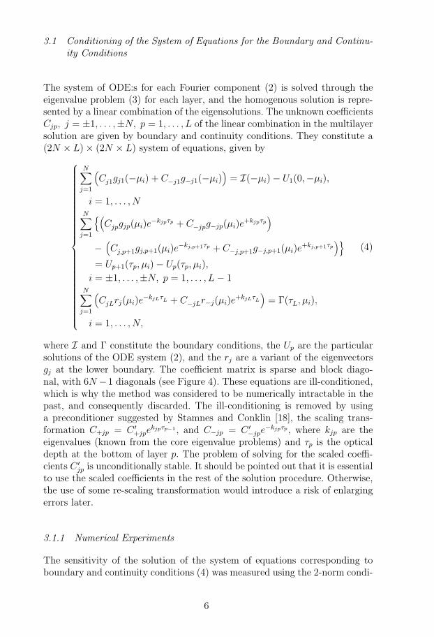
3.1 Conditioning of the System of Equations for the Boundary and Continu-ity Conditions
The system of ODE:s for each Fourier component (2) is solved through theeigenvalue problem (3) for each layer, and the homogenous solution is repre-sented by a linear combination of the eigensolutions. The unknown coefficientsCjp, j = ±1, . . . ,±N, p = 1, . . . , L of the linear combination in the multilayersolution are given by boundary and continuity conditions. They constitute a(2N × L) × (2N × L) system of equations, given by
⎧⎪⎪⎪⎪⎪⎪⎪⎪⎪⎪⎪⎪⎪⎪⎪⎪⎪⎪⎪⎪⎪⎪⎪⎪⎪⎪⎪⎨⎪⎪⎪⎪⎪⎪⎪⎪⎪⎪⎪⎪⎪⎪⎪⎪⎪⎪⎪⎪⎪⎪⎪⎪⎪⎪⎪⎩
N∑j=1
(Cj1gj1(−μi) + C−j1g−j1(−μi)
)= I(−μi) − U1(0,−μi),
i = 1, . . . , NN∑
j=1
{(Cjpgjp(μi)e
−kjpτp + C−jpg−jp(μi)e+kjpτp
)
−(Cj,p+1gj,p+1(μi)e
−kj,p+1τp + C−j,p+1g−j,p+1(μi)e+kj,p+1τp
)}= Up+1(τp, μi) − Up(τp, μi),
i = ±1, . . . ,±N, p = 1, . . . , L − 1N∑
j=1
(CjLrj(μi)e
−kjLτL + C−jLr−j(μi)e+kjLτL
)= Γ(τL, μi),
i = 1, . . . , N,
(4)
where I and Γ constitute the boundary conditions, the Up are the particularsolutions of the ODE system (2), and the rj are a variant of the eigenvectorsgj at the lower boundary. The coefficient matrix is sparse and block diago-nal, with 6N −1 diagonals (see Figure 4). These equations are ill-conditioned,which is why the method was considered to be numerically intractable in thepast, and consequently discarded. The ill-conditioning is removed by usinga preconditioner suggested by Stamnes and Conklin [18], the scaling trans-formation C+jp = C ′
+jpekjpτp−1 , and C−jp = C ′
−jpe−kjpτp , where kjp are the
eigenvalues (known from the core eigenvalue problems) and τp is the opticaldepth at the bottom of layer p. The problem of solving for the scaled coeffi-cients C ′
jp is unconditionally stable. It should be pointed out that it is essentialto use the scaled coefficients in the rest of the solution procedure. Otherwise,the use of some re-scaling transformation would introduce a risk of enlargingerrors later.
3.1.1 Numerical Experiments
The sensitivity of the solution of the system of equations corresponding toboundary and continuity conditions (4) was measured using the 2-norm condi-
6
tion number, defined as ‖A‖2‖A−1‖2 for a matrix A (see e.g. [8, section 2.7.2]).The condition number and the sparsity pattern of the coefficient matrix forthis system were studied with Dort2002 for a wide range of parameter sets(using the test problems [28] mentioned in section 3), with and without thepreconditioner, and with varying numbers of layers and Fourier componentnumbers. All different parameter sets gave very similar results, so only theresults of one set, which is representative for any of the other sets, are pre-sented here. The parameters of the presented test case were the following. Theillumination was a combination of diffuse light of intensity 0.3, and a beamof intensity 1.0 with polar angle cosine of 0.5 and azimuthal angle of π/2.The depth at the upper boundary was 0, and layer number p (using 1 to 10layers) had a thickness of 0.02/p. The underlying surface was diffuse, witha reflectance of 0.5. The medium had a scattering coefficient of 100 and anabsorption coefficient of 10, and had a Henyey-Greenstein [10] phase functionwith an asymmetry factor of 0.5. The calculations used 2N = 40.
3.1.2 Results
Figure 1 shows the condition number of the coefficient matrix for differentFourier component numbers and different numbers of layers after applyingthe preconditioner. Figure 2 is a slice from figure 1 for the single layer case.The plots show that the preconditioner works very well, giving a conditionnumber close to 1 in most cases, and around 30 in the worst case. Figure 3is the same as figure 2, but without the preconditioner (note the factor 10277
on the condition number axis scale), and shows that the problem is very ill-conditioned without the preconditioner, having a condition number near thelargest positive floating-point number for the system.
The sparsity pattern for the coefficient matrix after applying the precondi-tioner was generated with 2N = 40 and L = 5. This gives a 200 × 200 co-efficient matrix, and the single layer case can be obtained by extracting thetop left 40 × 40 sub-matrix. Figure 4 shows the coefficient matrix for the 0thFourier component, which has a special structure since it is the azimuthallyaveraged case. For all other Fourier component numbers, the structure is farsparser, although the bandwidth 6N − 1 is the same.
3.2 Conditioning of the Eigenvalue Problem
Certain choices concerning the properties of the phase function and the numer-ical quadrature give the eigenvalue problem (3) its symmetric structure, whichcan be exploited to increase the speed of the calculations. This is treated insection 4.1 below. However, since the eigenvalue problem is an important part
7
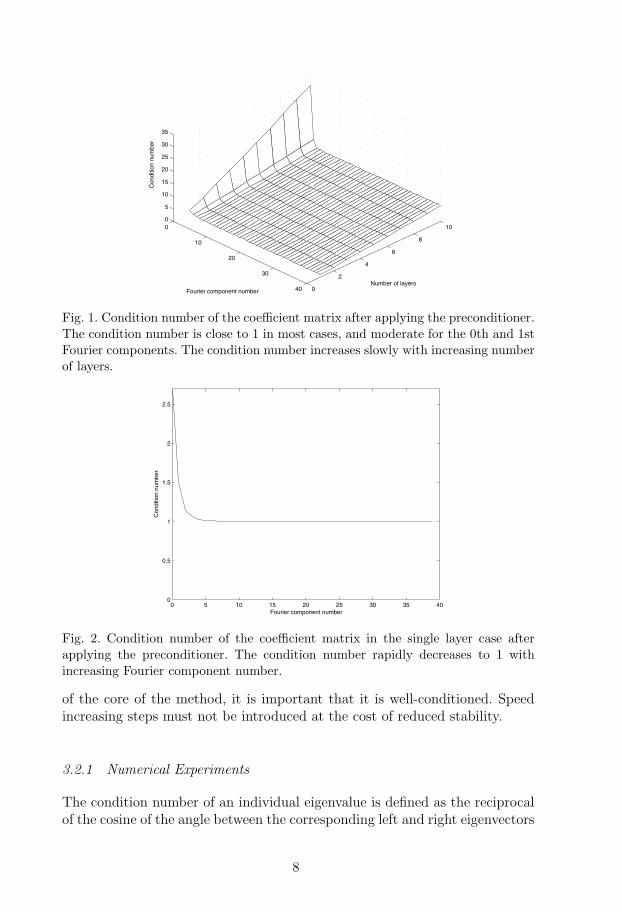
0
10
20
30
40 0
2
4
6
8
100
5
10
15
20
25
30
35
Number of layersFourier component number
Con
ditio
n nu
mbe
r
Fig. 1. Condition number of the coefficient matrix after applying the preconditioner.The condition number is close to 1 in most cases, and moderate for the 0th and 1stFourier components. The condition number increases slowly with increasing numberof layers.
0 5 10 15 20 25 30 35 400
0.5
1
1.5
2
2.5
Fourier component number
Con
ditio
n nu
mbe
r
Fig. 2. Condition number of the coefficient matrix in the single layer case afterapplying the preconditioner. The condition number rapidly decreases to 1 withincreasing Fourier component number.
of the core of the method, it is important that it is well-conditioned. Speedincreasing steps must not be introduced at the cost of reduced stability.
3.2.1 Numerical Experiments
The condition number of an individual eigenvalue is defined as the reciprocalof the cosine of the angle between the corresponding left and right eigenvectors
8
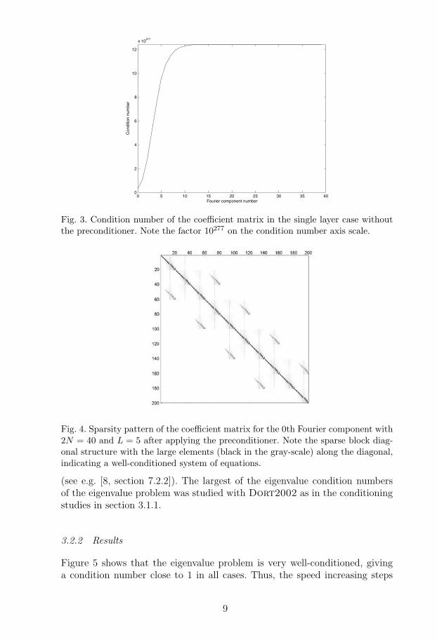
0 5 10 15 20 25 30 35 400
2
4
6
8
10
12
x 10277
Fourier component number
Con
ditio
n nu
mbe
r
Fig. 3. Condition number of the coefficient matrix in the single layer case withoutthe preconditioner. Note the factor 10277 on the condition number axis scale.
Fig. 4. Sparsity pattern of the coefficient matrix for the 0th Fourier component with2N = 40 and L = 5 after applying the preconditioner. Note the sparse block diag-onal structure with the large elements (black in the gray-scale) along the diagonal,indicating a well-conditioned system of equations.
(see e.g. [8, section 7.2.2]). The largest of the eigenvalue condition numbersof the eigenvalue problem was studied with Dort2002 as in the conditioningstudies in section 3.1.1.
3.2.2 Results
Figure 5 shows that the eigenvalue problem is very well-conditioned, givinga condition number close to 1 in all cases. Thus, the speed increasing steps
9
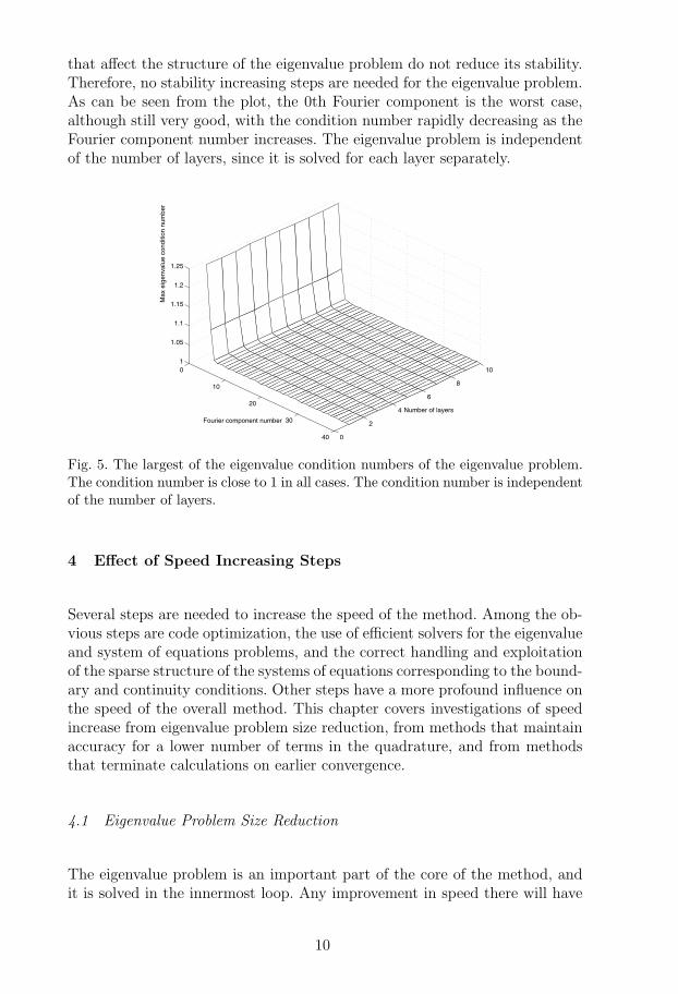
that affect the structure of the eigenvalue problem do not reduce its stability.Therefore, no stability increasing steps are needed for the eigenvalue problem.As can be seen from the plot, the 0th Fourier component is the worst case,although still very good, with the condition number rapidly decreasing as theFourier component number increases. The eigenvalue problem is independentof the number of layers, since it is solved for each layer separately.
0
10
20
30
40 0
2
4
6
8
101
1.05
1.1
1.15
1.2
1.25
Number of layers
Fourier component number
Max
eig
enva
lue
cond
ition
num
ber
Fig. 5. The largest of the eigenvalue condition numbers of the eigenvalue problem.The condition number is close to 1 in all cases. The condition number is independentof the number of layers.
4 Effect of Speed Increasing Steps
Several steps are needed to increase the speed of the method. Among the ob-vious steps are code optimization, the use of efficient solvers for the eigenvalueand system of equations problems, and the correct handling and exploitationof the sparse structure of the systems of equations corresponding to the bound-ary and continuity conditions. Other steps have a more profound influence onthe speed of the overall method. This chapter covers investigations of speedincrease from eigenvalue problem size reduction, from methods that maintainaccuracy for a lower number of terms in the quadrature, and from methodsthat terminate calculations on earlier convergence.
4.1 Eigenvalue Problem Size Reduction
The eigenvalue problem is an important part of the core of the method, andit is solved in the innermost loop. Any improvement in speed there will have
10
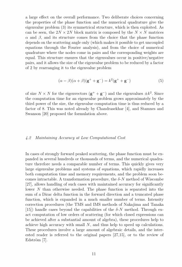
a large effect on the overall performance. Two deliberate choices concerningthe properties of the phase function and the numerical quadrature give theeigenvalue problem (3) its symmetrical structure, which is then exploited. Ascan be seen, the 2N × 2N block matrix is composed by the N × N matricesα and β, and its structure comes from the choice that the phase functiondepends on the scattering angle only (which makes it possible to get uncoupledequations through the Fourier analysis), and from the choice of numericalquadrature where the nodes come in pairs and the corresponding weights areequal. This structure ensures that the eigenvalues occur in positive/negativepairs, and it allows the size of the eigenvalue problem to be reduced by a factorof 2 by rearranging it to the eigenvalue problem
(α − β)(α + β)(g+ + g−) = k2(g+ + g−) (5)
of size N × N for the eigenvectors (g+ + g−) and the eigenvalues ±k2. Sincethe computation time for an eigenvalue problem grows approximately by thethird power of the size, the eigenvalue computation time is thus reduced by afactor of 8. This was noted already by Chandrasekhar [4], and Stamnes andSwanson [20] proposed the formulation above.
4.2 Maintaining Accuracy at Low Computational Cost
In cases of strongly forward peaked scattering, the phase function must be ex-panded in several hundreds or thousands of terms, and the numerical quadra-ture therefore needs a comparable number of terms. This quickly gives verylarge eigenvalue problems and systems of equations, which rapidly increasesboth computation time and memory requirements, and the problem soon be-comes intractable. A transformation procedure, the δ-N method of Wiscombe[27], allows handling of such cases with maintained accuracy for significantlylower N than otherwise needed. The phase function is separated into thesum of a Dirac delta function in the forward direction and a truncated phasefunction, which is expanded in a much smaller number of terms. Intensitycorrection procedures (the TMS and IMS methods of Nakajima and Tanaka[15]) handle cases beyond the capabilities of the δ-N method. Through ex-act computation of low orders of scattering (for which closed expressions canbe achieved after a substantial amount of algebra), these procedures help toachieve high accuracy with small N , and thus help to speed up calculations.These procedures involve a large amount of algebraic details, and the inter-ested reader is referred to the original papers [27,15], or to the review ofEdstrom [7].
11
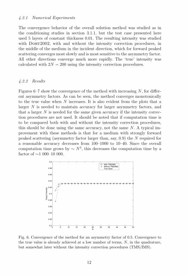
4.2.1 Numerical Experiments
The convergence behavior of the overall solution method was studied as inthe conditioning studies in section 3.1.1, but the test case presented hereused 5 layers of constant thickness 0.01. The resulting intensity was studiedwith Dort2002, with and without the intensity correction procedures, inthe middle of the medium in the incident direction, which for forward peakedscattering converges most slowly and is most sensitive to the asymmetry factor.All other directions converge much more rapidly. The ‘true’ intensity wascalculated with 2N = 200 using the intensity correction procedures.
4.2.2 Results
Figures 6–7 show the convergence of the method with increasing N , for differ-ent asymmetry factors. As can be seen, the method converges monotonicallyto the true value when N increases. It is also evident from the plots that alarger N is needed to maintain accuracy for larger asymmetry factors, andthat a larger N is needed for the same given accuracy if the intensity correc-tion procedures are not used. It should be noted that if computation time isto be compared both with and without the intensity correction procedures,this should be done using the same accuracy, not the same N . A typical im-provement with these methods is that for a medium with strongly forwardpeaked scattering (asymmetry factor larger than, say, 0.9) the N required fora reasonable accuracy decreases from 100–1000 to 10–40. Since the overallcomputation time grows by ∼ N3, this decreases the computation time by afactor of ∼1 000–10 000.
0 5 10 15 20 25 30 35 40 45 500.3
0.32
0.34
0.36
0.38
0.4
0.42
0.44
0.46
0.48
0.5
N
Out
put i
nten
sity
With TMS/IMSWithout TMS/IMSTrue value
Fig. 6. Convergence of the method for an asymmetry factor of 0.5. Convergence tothe true value is already achieved at a low number of terms, N , in the quadrature,but somewhat later without the intensity correction procedures (TMS/IMS).
12
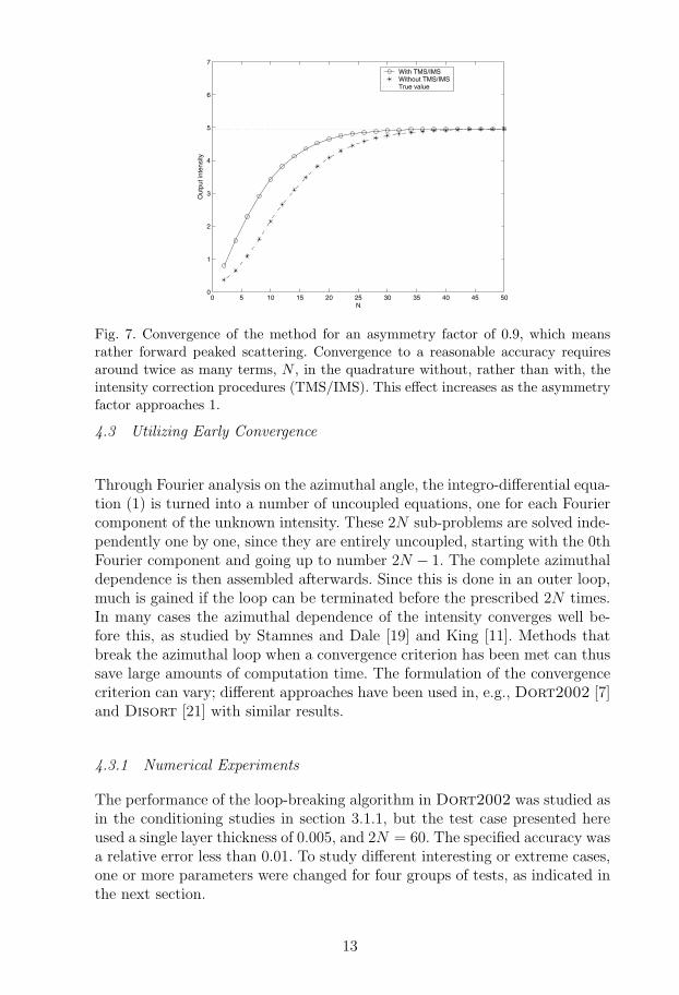
0 5 10 15 20 25 30 35 40 45 500
1
2
3
4
5
6
7
N
Out
put i
nten
sity
With TMS/IMSWithout TMS/IMSTrue value
Fig. 7. Convergence of the method for an asymmetry factor of 0.9, which meansrather forward peaked scattering. Convergence to a reasonable accuracy requiresaround twice as many terms, N , in the quadrature without, rather than with, theintensity correction procedures (TMS/IMS). This effect increases as the asymmetryfactor approaches 1.
4.3 Utilizing Early Convergence
Through Fourier analysis on the azimuthal angle, the integro-differential equa-tion (1) is turned into a number of uncoupled equations, one for each Fouriercomponent of the unknown intensity. These 2N sub-problems are solved inde-pendently one by one, since they are entirely uncoupled, starting with the 0thFourier component and going up to number 2N − 1. The complete azimuthaldependence is then assembled afterwards. Since this is done in an outer loop,much is gained if the loop can be terminated before the prescribed 2N times.In many cases the azimuthal dependence of the intensity converges well be-fore this, as studied by Stamnes and Dale [19] and King [11]. Methods thatbreak the azimuthal loop when a convergence criterion has been met can thussave large amounts of computation time. The formulation of the convergencecriterion can vary; different approaches have been used in, e.g., Dort2002 [7]and Disort [21] with similar results.
4.3.1 Numerical Experiments
The performance of the loop-breaking algorithm in Dort2002 was studied asin the conditioning studies in section 3.1.1, but the test case presented hereused a single layer thickness of 0.005, and 2N = 60. The specified accuracy wasa relative error less than 0.01. To study different interesting or extreme cases,one or more parameters were changed for four groups of tests, as indicated inthe next section.
13
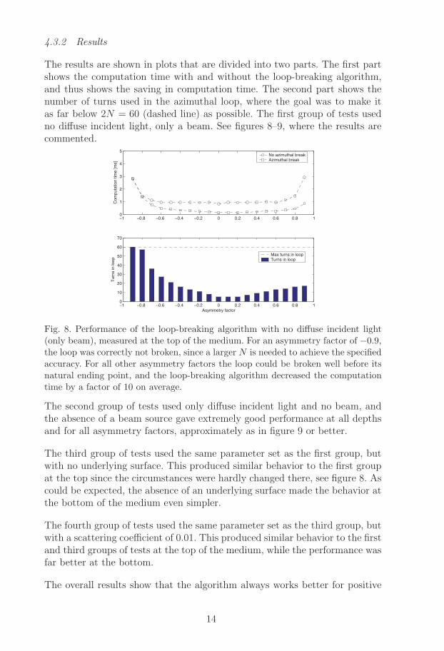
4.3.2 Results
The results are shown in plots that are divided into two parts. The first partshows the computation time with and without the loop-breaking algorithm,and thus shows the saving in computation time. The second part shows thenumber of turns used in the azimuthal loop, where the goal was to make itas far below 2N = 60 (dashed line) as possible. The first group of tests usedno diffuse incident light, only a beam. See figures 8–9, where the results arecommented.
−1 −0.8 −0.6 −0.4 −0.2 0 0.2 0.4 0.6 0.8 10
1
2
3
4
5
Com
puta
tion
time
[ms]
−1 −0.8 −0.6 −0.4 −0.2 0 0.2 0.4 0.6 0.8 10
10
20
30
40
50
60
70
Asymmetry factor
Tur
ns in
loop
Max turns in loopTurns in loop
No azimuthal breakAzimuthal break
Fig. 8. Performance of the loop-breaking algorithm with no diffuse incident light(only beam), measured at the top of the medium. For an asymmetry factor of −0.9,the loop was correctly not broken, since a larger N is needed to achieve the specifiedaccuracy. For all other asymmetry factors the loop could be broken well before itsnatural ending point, and the loop-breaking algorithm decreased the computationtime by a factor of 10 on average.
The second group of tests used only diffuse incident light and no beam, andthe absence of a beam source gave extremely good performance at all depthsand for all asymmetry factors, approximately as in figure 9 or better.
The third group of tests used the same parameter set as the first group, butwith no underlying surface. This produced similar behavior to the first groupat the top since the circumstances were hardly changed there, see figure 8. Ascould be expected, the absence of an underlying surface made the behavior atthe bottom of the medium even simpler.
The fourth group of tests used the same parameter set as the third group, butwith a scattering coefficient of 0.01. This produced similar behavior to the firstand third groups of tests at the top of the medium, while the performance wasfar better at the bottom.
The overall results show that the algorithm always works better for positive
14
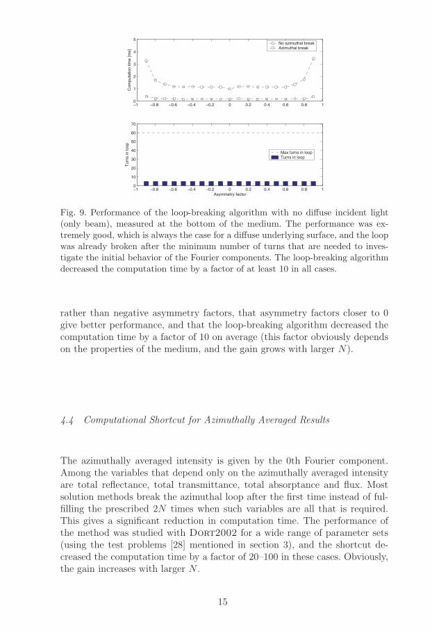
−1 −0.8 −0.6 −0.4 −0.2 0 0.2 0.4 0.6 0.8 10
1
2
3
4
5
Com
puta
tion
time
[ms]
−1 −0.8 −0.6 −0.4 −0.2 0 0.2 0.4 0.6 0.8 10
10
20
30
40
50
60
70
Asymmetry factor
Tur
ns in
loop
Max turns in loopTurns in loop
No azimuthal breakAzimuthal break
Fig. 9. Performance of the loop-breaking algorithm with no diffuse incident light(only beam), measured at the bottom of the medium. The performance was ex-tremely good, which is always the case for a diffuse underlying surface, and the loopwas already broken after the minimum number of turns that are needed to inves-tigate the initial behavior of the Fourier components. The loop-breaking algorithmdecreased the computation time by a factor of at least 10 in all cases.
rather than negative asymmetry factors, that asymmetry factors closer to 0give better performance, and that the loop-breaking algorithm decreased thecomputation time by a factor of 10 on average (this factor obviously dependson the properties of the medium, and the gain grows with larger N).
4.4 Computational Shortcut for Azimuthally Averaged Results
The azimuthally averaged intensity is given by the 0th Fourier component.Among the variables that depend only on the azimuthally averaged intensityare total reflectance, total transmittance, total absorptance and flux. Mostsolution methods break the azimuthal loop after the first time instead of ful-filling the prescribed 2N times when such variables are all that is required.This gives a significant reduction in computation time. The performance ofthe method was studied with Dort2002 for a wide range of parameter sets(using the test problems [28] mentioned in section 3), and the shortcut de-creased the computation time by a factor of 20–100 in these cases. Obviously,the gain increases with larger N .
15
5 Verification of Accuracy after Speed Increasing Steps
It is essential that the steps included to increase the speed of a method donot compromise the accuracy. To verify this, a series of tests were performed.Results with the speed increasing steps were compared to reference valuesobtained without the speed increasing steps and with large N for accuracy.
5.1 Numerical Experiments
The accuracy of the speed increasing steps were studied for a wide range ofparameter sets (using the test problems [28] mentioned in section 3). The testproblems come with both input and output values, and most problems canalso be compared with published results that are referred to in the test suite.The different test cases include accuracy and consistency checks, variation ofall parameters, and cases with a risk of breakdown due to extreme values ofthe input parameters.
5.2 Results
The comparisons gave very good agreement in all test cases without excep-tion. The deviations from reference values of results obtained with the speedincreasing steps were never larger than the round-off error in the given data.This provides substantial support for the accuracy of the tested speed in-creasing steps, and thus indicates that they are not introduced at the cost ofreduced accuracy.
6 Suggestions for Future Work
The intensity correction procedures (the TMS and IMS methods) take al-most no extra time in themselves. However, for very forward scattering media(asymmetry factor close to 1), they utilize values of the normalized associatedLegendre functions, Λm
l , for indices l and m from 1 to fairly large numbers,and the computation time of all these evaluations becomes noticeable. Anystudies that result in faster ways of evaluation of Λm
l for indices l and m from1 up to a few hundreds would be welcome.
Another improvement that will have a significant effect on the overall perfor-mance is to speed up the computation of the eigenvalue problem. As discussedby Stamnes et al. [22], the reduced matrix is real and non-symmetric, but in
16
spite of this is known to have real eigenvalues. They showed that it is possibleto make the matrix symmetrical, but their method introduced extra com-putational cost as well as round-off errors due to the matrix multiplicationsinvolved in the transformations. Since the numerical solution of the eigenvalueproblem is a critical and time-consuming part of the discrete ordinate method,a faster method that avoids the use of complex arithmetic — without loss ofaccuracy or efficiency — would be a welcome improvement.
7 Discussion
This paper gives a systematic presentation of the effect of the steps that areneeded or possible to make any discrete ordinate radiative transfer solutionmethod numerically efficient. To the author’s knowledge, this has not beensummarized in one single publication before. This is done through studiesof the numerical performance of the stability enhancing and speed increas-ing steps used in modern discrete ordinate radiative transfer algorithms. Thesolution method Dort2002 by Edstrom [7] is used in the tests, since it is de-signed for methodical numerical experiments through its modularized designand ability to give any kind of intermediate results and performance data.
The system of equations corresponding to boundary and continuity condi-tions is very ill-conditioned, with a condition number near the largest positivefloating-point number for the system. It is shown that after applying the pre-conditioner, the condition number is close to 1 in most cases, and around 30in the worst test case. It is also shown that the preconditioner preserves thesparsity pattern, which is used to solve the system of equations efficiently.This indicates that the preconditioner works very well, and yields a system ofequations well suited for numerical solution.
The symmetric structure of the eigenvalue problem allows reducing its size bya factor of 2, and thus the eigenvalue computation time by a factor of 8. It isshown that the reduced eigenvalue problem is very well-conditioned, giving acondition number close to 1, so this reduction is not introduced at the cost ofreduced stability.
The convergence behavior of the method is illustrated. The intensity correctionprocedures make it possible to maintain accuracy for significantly lower N thanotherwise needed. It is shown that this typically decreases the computationtime by a factor of ∼1 000–10 000 in cases with strongly forward peakedscattering.
It is shown that algorithms for breaking the azimuthal loop, based on a con-vergence criterion, on the average decrease the computation time by a factor
17
of 10. The gain grows with larger N , and also depends on the properties ofthe medium.
A computational shortcut, implemented to allow for much faster calculationof variables that depend only on the azimuthally averaged intensity, makes itpossible to break the azimuthal loop after the first time instead of fulfilling theprescribed 2N times. It is shown that the shortcut decreases the computationtime by a factor of 20–100 when 2N = 40. Obviously, the gain increases withlarger N .
Different sets of relevant test problems are solved with and without the speedincreasing steps. It is shown, by comparing the results, that the agreementis invariably very good. This provides substantial support for the accuracy ofthe tested speed increasing steps, and thus shows that they are not introducedat the cost of reduced accuracy.
The performance tests illustrate the effect of the steps that are taken to im-prove the stability and speed of the method. It is shown how the steps togethergive an unconditionally stable solution procedure to a problem previously con-sidered numerically intractable, and how they together decrease the compu-tation time compared to a naive implementation by a factor 1 000–10 000in typical cases and by a factor up to and beyond 10 000 000 in extremecases. Further studies and developments, which can have a positive impact oncomputation time, are suggested.
Acknowledgements
The author wishes to thank Marcus Lehto for preparing most of the Matlab
scripts used in the performance tests.
References
[1] M. Abramowitz and I. A. Stegun, Handbook of Mathematical Functions,National Bureau of Standards, Applied Mathematics Series, Volume 55, 1964(reprinted by Dover, New York, 1968).
[2] S. Chandrasekhar, On the Radiative Equilibrium of a Stellar Atmosphere,Astrophys. J. 99 (1944) 180–190.
[3] S. Chandrasekhar, On the Radiative Equilibrium of a Stellar Atmosphere II,Astrophys. J. 100 (1944) 76–86.
[4] S. Chandrasekhar, Radiative Transfer, Dover, New York, 1960.
18
[5] J. V. Dave and B. Armstrong, Computations of high-order AssociatedLegendre Polynomials, J. Quant. Spectrosc. Radiat. Transfer 10 (1970) 557–562.
[6] P. Davis and P. Rabinowitz, Methods of Numerical Integration, AcademicPress, New York, 1975, 1984.
[7] P. Edstrom, A Fast and Stable Solution Method for the Radiative TransferProblem, SIAM Rev. 47 (2005) 447–468.
[8] G. H. Golub and C. F. Van Loan, Matrix Computations, 3rd ed., JohnsHopkins University Press, Baltimore, 1996.
[9] G. H. Golub and J. H. Welsch, Calculation of Gauss Quadrature Rules,Math. Comp. 23 (1969) 221–230.
[10] L. G. Henyey and J. L. Greenstein, Diffuse Radiation in the Galaxy,Astrophys. J. 93 (1941) 70–83.
[11] M. D. King, Number of Terms Required in the Fourier Expansion of theReflection Function for Optically Thick Atmospheres, J. Quant. Spectrosc.Radiat. Transfer 30 (1983) 143–161.
[12] W. Magnus and F. Oberhettinger, Formulas and Theorems for theFunctions of Mathematical Physics, Chelsea, New York, 1949.
[13] P. S. Mudgett and L. W. Richards, Multiple Scattering Calculations forTechnology, Appl. Opt. 10 (1971) 1485–1502.
[14] P. S. Mudgett and L. W. Richards, Multiple Scattering Calculations forTechnology II, J. Colloid Interf. Sci. 39 (1972) 551–567.
[15] T. Nakajima and M. Tanaka, Algorithms for Radiative IntensityCalculations in Moderately Thick Atmospheres Using a Truncation Approach,J. Quant. Spectrosc. Radiat. Transfer 40 (1988) 51–69.
[16] A. Schuster, Radiation Trough a Foggy Atmosphere, Astrophys. J., 21 (1905)1–22. (Reprinted in D. H. Menzel (Ed.), Selected Papers on the Transfer ofRadiation, Dover, New York, 1966, pp.3–24.)
[17] K. Stamnes, On the computation of angular distributions of radiation inplanetary atmospheres, J. Quant. Spectrosc. Radiat. Transfer 28 (1982) 47–51.
[18] K. Stamnes and P. Conklin, A new multi-layer discrete ordinate approach toradiative transfer in vertically inhomogeneous atmospheres, J. Quant. Spectrosc.Radiat. Transfer 31 (1984) 273–282.
[19] K. Stamnes and H. Dale, A new look at the discrete ordinate methodfor radiative transfer calculation in anisotropically scattering atmospheres. II:Intensity computations, J. Atmos. Sci. 38 (1981) 2696–2706.
[20] K. Stamnes and R. A. Swanson, A new look at the discrete ordinate methodfor radiative transfer calculations in anisotropically scattering atmospheres, J.Atmos. Sci. 38 (1981) 387–399.
19
[21] K. Stamnes, S-C. Tsay and I. Laszlo, DISORT, a General-Purpose FortranProgram for Discrete-Ordinate-Method Radiative Transfer in Scattering andEmitting Layered Media, NASA report, 2000.
[22] K. Stamnes, S.-C. Tsay and T. Nakajima, Computation of eigenvalues andeigenvectors for discrete ordinate and matrix operator method radiative transfer,J. Quant. Spectrosc. Radiat. Transfer 39 (1988) 415–419.
[23] K. Stamnes, S-C. Tsay, W. Wiscombe, and K. Jayaweera, NumericallyStable Algorithm for Discrete-Ordinate-Method Radiative Transfer in MultipleScattering and Emitting Layered Media, Appl. Opt. 27 (1988) 2502–2509.
[24] J. B. Sykes, Approximate Integration of the Equation of Transfer, Mon. Not.Roy. Astron. Soc. 111 (1951) 377–386.
[25] G. E. Thomas and K. Stamnes, Radiative Transfer in the Atmosphere andOcean, Cambridge University Press, 1999.
[26] G. C. Wick, Uber ebene Diffusionsprobleme, Z. Phys. 120 (1943) 702–718.
[27] W. J. Wiscombe, The Delta-M Method: Rapid Yet Accurate Radiative FluxCalculations for Strongly Asymmetric Phase Functions, J. Atmos. Sci. 34 (1977)1408–1422.
[28] The DISOTEST files in the DISORT2.0beta folder at the Disort web site:ftp://climate1.gsfc.nasa.gov/wiscombe/Multiple_Scatt/.
20
III

397Nordic Pulp and Paper Research Journal Vol 19 no. 3/2004
KEYWORDS: Light scattering, Mathematical models,Radiative transfer, Kubelka-Munk, Light absorption, Errors,Reflectance calculations.
SUMMARY: The need for optical modeling of paper is obviousto provide connections between its optical response and theactual properties of the paper. It is argued that modern solutionmethods from radiative transfer theory could be consideredinstead of the Kubelka-Munk model, and a specific example,DORT2002, is tested. It is shown that Kubelka-Munk is a sim-ple special case of DORT2002, and the two models and theircoefficients are compared. A comprehensive list of advantagesfor the applied user of a model with higher dimensionality issupplied.
It is shown, by the use of DORT2002, that when themedium has finite thickness, the light distribution deviates fromthe perfectly diffuse even under the theoretically ideal condi-tions for which Kubelka-Munk was created. This effect causeserrors in Kubelka-Munk reflectance calculations that may be upto 20% and more, even for a grammage of 80 g/m2. The magni-tude of the error shows a strong dependence on the degree oflight absorption, with higher absorption giving greater error.DORT2002 can well be considered for increased understandingin cases where the level of accuracy of Kubelka-Munk reflec-tance calculations is not sufficient.
ADDRESS OF THE AUTHOR: Per Edström([email protected]): Department of Technology, Physics andMathematics, Mid Sweden University, SE-871 88 Härnösand,Sweden.
1. IntroductionAs is well known, the Kubelka-Munk light scattering andlight absorption coefficients (s and k) are widely used inthe pulp and paper industry in applications ranging fromresearch projects to practical problems in paper mills.Examples are prediction of brightness and opacity ofpapers containing different pulps and fillers, or paperswith multilayer structures (coated and printing papers).These coefficients provide a link between the (measured)reflectance factor, e.g. brightness, and properties of thepaper sample, so that the reasons for a high or lowreflectance may be better understood. The s- and k-valuesare also linked to unit operations in pulp and papertechnology through many investigations over the years.The reasons for this extensive use of the Kubelka-Munkmodel are most likely the simplicity of the equations(which was a major advantage before the introduction ofpersonal computers) and the fact that they are invertible,roughly meaning that reflectance values can be calculatedfrom s and k, and that s and k can be calculated fromreflectance values.
However, the Kubelka Munk equations are a specialcase of a solution method to what is known as the
radiative transfer problem. Given the fast development ofpersonal computers, it is worthwhile to investigate othersolution methods that give a more detailed and moreaccurate description of the paper sample, and yet caneasily be made accessible for the applied user.
Radiative transfer theory describes the interaction ofradiation with scattering and absorbing media. It hasbeen applied to such different applications as stellaratmospheres, infrared and visible light in space and theatmosphere, optical tomography and diffusion ofneutrons. An industrially important application is lightscattering in textile, paint, pigment films, paper and print,and accurate calculation methods are crucial for thesesectors of industry.
Discrete ordinate solution methods for radiativetransfer problems have been studied throughout the lastcentury. The first approximate solution to the radiativetransfer problem was presented by Schuster (1905), whoconsidered radiation only in a forward and a backwarddirection. Clearly influenced by this, Kubelka and Munk(1931) developed their well-known model, which wasfurther refined by Kubelka (1948; 1954). The modelspresented by Schuster and Kubelka and Munk, and othersafter them, are known as two-flux models.
By expressing an integral as a finite sum, what is nowknown as numerical quadrature, Wick (1943) gave thefirst general treatment of discrete ordinate methods forthe radiative transfer problem. The terms in the sum canbe interpreted as the contribution to flux or intensityfrom a discrete cone in spherical geometry. The polarangles of these cones are referred to as discrete ordinates,which has given the method its name, and the cones arecalled channels or streams. Using only two channelsgives the earlier two-flux methods. If more channels areused, the methods are referred to as multi-flux methodsor many-flux methods. Chandrasekhar (1944a) describeda method using spherical harmonics, but having readWick’s article, he adopted the discrete ordinate method,and further refined it (1944b). Later, he wrote a classicexposition on radiative transfer theory in book form(Chandrasekhar 1960), and since then the area hasexpanded tremendously.
Along with this expansion, there has been a continuousdevelopment of solution methods for the radiativetransfer problem. When Kubelka and Munk presentedtheir model, it was state-of-the-art, but now it should beseen as the approximation it is. Several limitations for theKubelka-Munk model have been reported, for exampleconcerning dependencies between the s and k coefficientsfor translucent or strongly absorbing media (Foote 1939;Nordman et al. 1966; Moldenius 1983; Rundlöf andBristow 1997), and attempts have been made to attributesome of this behavior to intrinsic errors of – or pheno-
Comparison of the DORT2002 radiative transfer solutionmethod and the Kubelka-Munk modelPer Edström, Department of Technology, Physics and Mathematics, Mid Sweden University, Härnösand
398 Nordic Pulp and Paper Research Journal Vol 19 no. 3/2004
mena not included in – the Kubelka-Munk model (vanden Akker 1966; van den Akker 1968; Koukoulas andJordan 1997; Granberg and Edström 2003). Despite theselimitations, the Kubelka-Munk model is in widespreaduse for multiple scattering calculations in paper, papercoatings, printed paper, paint, plastic and textile, proba-bly due to its explicit form and ease of use. These are alsoreasons for the continued usage where the accuracy issufficient, and where there are no reported limitations.However, new solution methods with better accuracy anda larger range of applicability should be considered inmany cases.
The DORT2002 software is a fast and accurate tool forsolving radiative transfer problems in vertically inhomo-geneous turbid media, using a discrete ordinate modelgeometry. DORT2002 is implemented in MATLAB, andis adapted to light scattering simulations in paper andprint. The model was presented in a recent paper byEdström (2003), which thoroughly describes the modeland its features. Accuracy and numerical performance ofDORT2002 have been evaluated by Edström (2004), andthe solution method was found to be accurate, very fast,and numerically stable.
The purpose of this paper is to draw attention to thepotential of models of higher dimensionality, for examplethose provided by radiative transfer theory, since moderncomputers make it fully tractable to use such models. Inthis paper, DORT2002 is used as an example of suchmodels. Section 2 of this paper gives a short outline of aradiative transfer formulation of the light scattering pro-blem, and in section 3 a translation between the coeffici-ents of the Kubelka-Munk and DORT2002 models isgiven, together with a discussion of when the translationis valid. Section 4 covers the application of Kubelka-Munk and DORT2002 to a number of test problems, pro-vides and discusses important numerical results, and spe-cifically notes that Kubelka-Munk may fail to providecorrect results even under ideal conditions. Section 5supplies a list of advantages for the applied user of amodel with higher dimensionality, and notes that theangular resolution of DORT2002 enables it to exceedKubelka-Munk extensively by giving a more detailed andmore accurate description of the paper sample. Finally,some concluding discussions and references are given.
2. The physical problemFor an ideally reflecting medium, all incoming light isspecularly reflected at the surface. For a turbid medium,transmission as well as absorption and multiple scatteringinside the medium have to be taken into consideration. Inthis paper, the problem is studied in plane-parallelgeometry, where the horizontal extension of the mediumis assumed to be large enough to give no boundaryeffects at the sides. The boundary conditions at the topand bottom boundary surfaces, including illumination,are assumed to be time- and space-independent on therespective boundary surface. The radiation is assumed tobe monochromatic, or confined to a sufficiently narrowwavelength range to make scattering and absorptionconstant. The scattering is assumed to be conservative,
i.e. without change in frequency between incoming andoutgoing radiation. The medium is treated as a continuumof scattering and absorption sites. Kubelka-Munk andDORT2002 both use these same assumptions about themedium. The main difference is that Kubelka-Munk islimited to diffuse illumination and scattering, whileDORT2002 handles any illumination and any scatteringthanks to the angle-resolved model geometry. DORT-2002 provides this resolution by dividing the space intoany number of “channels”, corresponding to differentdirections, while Kubelka-Munk only considers the ave-raged directions “up” and “down”.
The energy flow is thought of as non-interacting beamsof radiation in all directions. This makes it possible totreat the beams separately. The intensity, I, of theradiation is always considered to be positive. Whenradiation traverses the infinitesimal thickness ds of themedium in its direction of propagation, a fraction isextinct due to absorption and scattering. The intensitythen becomes I + dI, and the extinction coefficient isdefined as σe = -
dI–Ids. The extinction coefficient can beseparated into two parts, called the absorption and scatte-ring coefficients, σa and σs, corresponding to the twodifferent origins of the extinction. They are related to theextinction coefficient through σe = σa +σs . It should benoted that these coefficients are real physical quantities,and not defined through a model equation such as theKubelka-Munk s and k. A convenient measure is thesingle scattering albedo, which is the probability forscattering given an extinction event, and is defined as a =σs / σe=σs / (σa+σs ).
The phase function, p, specifies the angular distribution ofthe scattered radiation. If the phase function is normalized by
where θ and ϕ are the polar and azimuthal angle coordi-nates of spherical geometry for the direction of the radia-tion (in the remainder of this paper, primed argumentscorrespond to incident radiation), this can be given a pro-babilistic interpretation. Given that radiation in the direc-tion (θ´,ϕ´) is scattered, the probability that it is scatteredinto the cone of solid angle dθdϕ centered on the direc-tion (θ,ϕ) is
It is common that the shape of the scattering probability-distribution is controlled by a parameter in the phasefunction, an asymmetry factor.
For plane-parallel geometry, it is convenient tomeasure distances normal to the surface of the medium.This coincides with the z-axis in a Cartesian coordinatesystem if the surface is placed in the x-y-plane, and it isevident that dz = ds cosθ. The optical depth, measuredfrom the top surface and down, is then defined as
It is also common to introduce u= cosθ (and someti-mes μ = |cosθ |), which gives dτ = -σ euds . Chandrasekhar(1960, eq. I.71) states the equation of radiative transfer
399Nordic Pulp and Paper Research Journal Vol 19 no. 3/2004
for a scattering plane-parallel medium as
The integral term on the right hand side is a sourcefunction. It gives the intensity scattered from all inco-ming directions at a point to a specified direction.
3. A comparison between the coefficients of theKubelka-Munk and DORT2002 models The aim of this section is to make a comparison of thescattering and absorption coefficients s and k of theKubelka-Munk model, and the real physical quantities σs
and σa – also known as cross sections – used in radiativetransfer, and to specify under what conditions an exacttranslation is valid. Since the coefficients of the Kubelka-Munk model are so well known and in such widespreaduse, a translation between these is valuable for the futureuse of both model types.
The Kubelka-Munk equations can be written
where i is the intensity in the downward direction and j isthe intensity in the upward direction. s and k are the lightscattering and absorption coefficients, and x is thedistance measured from the background and upwards.This can be rewritten as
The first term on the right hand side is absorption, i.e. theintensity “disappears”, the second term is intensityscattered into the opposite direction, and the third term isa contribution to the intensity, scattered from the oppositedirection. The derivation of the Kubelka-Munk equationsassumes that the light is perfectly diffuse, but the fact thatlight incident at an angle has a longer optical path to acertain depth in the medium is not explicitly considered(or it can be assumed to be built into the coefficients sand k). Hence, k is the part of the intensity that is absor-bed and “disappears” upon passage of the infinitesimalthickness dx of the medium. s is the part of the intensitythat is scattered to the opposite direction upon passage ofthe infinitesimal thickness dx of the medium.
As mentioned previously, the DORT2002 model is amore general model than Kubelka-Munk. In the simplespecial case with only two channels, corresponding to theonly two directions “up” and “down” of Kubelka-Munk,the DORT2002 equations can be rewritten as
where i and j generally depend on τ and μ. In the discrete
ordinate approximation (using Double-Gauss numericalquadrature) for two channels, i(τ, μ) and j(τ, μ) are repla-ced with their hemispherical averages, i(τ) and j(τ). Fordiffuse light, the average of μ becomes
It should be noted here, that the distance x used inKubelka-Munk, and the optical depth τ used inDORT2002 are in opposite directions. Therefore, dτ = -σe
dx = -(σa + σs )dx , and the DORT2002 equations become
Here the equations have been written in this form forease of comparison. The first term on the right hand sideis absorption, i.e. the intensity “disappears”, and thesecond term is totally scattered intensity. The third termis a contribution to the intensity, “scattered” from thesame direction, and the fourth term is a contribution tothe intensity, scattered from the opposite direction.Together the second and third terms form the netscattered intensity to the opposite direction. The fact thatlight incident at an angle has a longer optical path to acertain depth in the medium is explicitly considered, andthe effect is the factor 1/2 from the average of μ. Hence,2σa is the part of the intensity that is absorbed and “dis-appears” upon passage of the infinitesimal thickness dxof the medium. σs is the part of the intensity that is scat-tered to the opposite direction upon passage of the infini-tesimal thickness dx of the medium.
The conditions, under which an exact translation bet-ween the coefficients of the Kubelka-Munk and theDORT2002 models is valid, are: perfectly diffuse light,perfectly isotropic scattering, and only two channels inthe DORT2002 model. Under these conditions it isobvious from the calculations above that the followingrelations hold: k =2σa and s =σs.
The three validity conditions each deserve a short dis-cussion. First, if the light has an angular distributionother than perfectly diffuse, the average of μ is changed.Thus Eq (5) is not valid, and Eq (4) does not yield Eq (6).Second, if the scattering is anisotropic, the phase functionis no longer ≡1, and the integrals in Eq (4), where thephase function is implicitly present, are changed so thatthey are no longer the hemispherical average. Thus, Eq(4) does not yield Eq (6). The third validity condition,which is an effect of the finite thickness of the medium,deserves a longer discussion, which is contained in thesection on application tests. Here it can simply be notedthat in the case of more than two channels, Eq (4)becomes the far more complicated Eq (1), and a simpletranslation to Eq (6) is not possible.
There remains one more comment to give on coeffici-ents at this point; van den Akker (1949) showed that theKubelka-Munk differential equations remain unchangedif the original scattering and absorption coefficients S
400 Nordic Pulp and Paper Research Journal Vol 19 no. 3/2004
and K (unit m-1) are replaced by the specific scatteringand absorption coefficients s and k (unit m2
•kg-1), and thethickness X is replaced by weight per unit area (gramma-ge) W. He proposed that these should be used instead,based on the fact that in practical application of theKubelka-Munk model, the thickness of a paper maychange significantly without affecting the reflectance,suggesting that the light scattering remains unchanged,which naturally is also true for the grammage. The use ofgrammage is now common practice in paper-relatedapplications. All relationships are unaffected by this. Thissame convention is readily applied to the DORT2002model. Although derived for scattering and absorptioncoefficients with unit m-1 and optical depth τ , theequations remain unchanged if specific scattering andabsorption coefficients with unit m2
•kg-1 are used instead,together with the grammage W. As for the Kubelka-Munkmodel, all relationships are unaffected by this. It shouldbe noted that for both Kubelka-Munk and DORT2002,this can only be done if the scattering and absorptioncoefficients as well as the density of the medium areconstants. Otherwise the specific scattering and absorp-tion coefficients as well as the grammage will not beconstants, which is assumed by the theory.
4. Application tests of the Kubelka-Munk andDORT2002 models The two-channel case Theoretically, Kubelka-Munk is the simple two channelspecial case for DORT2002 if illumination, phasefunction and underlying surface are perfectly diffuse.Therefore, DORT2002 should yield results identical toKubelka-Munk under these conditions. This was testedfor various scattering and absorption coefficients anddifferent thicknesses/grammages by calculating totalreflectance for a medium over a black background, R0 ,and over an opaque pad of the medium itself, R∞. TheKubelka-Munk calculations were done according to theequations in Pauler (2002). The definitions for thescattering and absorption coefficients differ betweenKubelka-Munk (s and k) and DORT2002 (σs and σa ), sothe relations given in the previous section were used fortranslation. Table 1 gives the parameter values used, andall combinations were tested, giving a total of 27 testcases. The parameter values were chosen so that thecombinations would represent a range of paper qualities,both unprinted, dyed and printed.
In all 27 test cases, Kubelka-Munk gave identicalresults to DORT2002, when only two channels were used,as should be expected. This verifies that DORT2002indeed becomes Kubelka-Munk when using only twochannels.
The multi-channel case:Effects of finite medium thicknessIt is now tempting to think that if illumination, phasefunction and underlying surface were perfectly diffuse,the resulting light distribution would be perfectly diffuse.There would therefore be no need for DORT2002 in thiscase at all, since with two channels it gives identicalresults to Kubelka-Munk. However, this is wrong. Thelight distribution deviates from the perfectly diffuse dueto the finite thickness of the medium, since some lightescapes through the lower boundary. With more channels,say twenty, DORT2002 detects and quantifies this.
It is important to realize that scattering is a localphenomenon, and even if every scattering event isperfectly diffuse, the total scattered light distributionneeds not be perfectly diffuse due to edge effects.Kubelka and Munk did not recognize this fact in the firstpaper on their model. They assume infinite horizontalextension to avoid edge effects, but do not consider edgeeffects due to finite thickness. Even the follow-up paperby Kubelka (1948), that aims to theoretically derive arange of validity for that model, does not recognize thisfact but rather assumes the opposite line of reasoning:“Practically it will be so when the illumination is aperfectly diffuse one and when the material formingspecimens of different thickness reflects and transmitsalways perfectly diffused light only”. This is an intui-tively tempting belief, but it is not true when the mediumhas finite thickness since some light escapes through thelower boundary, and the light distribution becomesslightly changed. Kubelka (1948) defines u dx and v dxas the average path of the light passing through the layerdx going down and up, respectively, taking into conside-ration the various directions of the beams of radiation.Kubelka is right when he states that the model is validwhen u = v = const, but wrong when he assumes thatu = v = const if scattering and illumination are perfectlydiffuse – it will still not be true for a medium of finitethickness.
This effect is far from negligible, and can sometimesbe very large indeed. This is illustrated by Table 2, whichpresents the results of the same 27 test cases as in theprevious section, but now using twenty channels inDORT2002. This can be considered to be a true value,since simple tests show that DORT2002 has alreadyconverged (it has been shown by Edström (2004) thatDORT2002 converges to the true value when the numberof channels increases).
From Table 2 it is clear that the magnitude of therelative error shows a strong dependence on the degree ofabsorption, with higher absorption giving greater relativeerror. There is also a weak dependence on the degree ofscattering, higher scattering giving somewhat smallerrelative error. This is in accordance with earlier papersthat address problems when using Kubelka-Munk ontranslucent or strongly absorbing media (Foote 1939;Nordman et al. 1966; Moldenius 1983; Rundlöf andBristow 1997). Thus, DORT2002 offers a partial explana-tion to these previously reported problems, as it quantifi-es the deviation from perfectly diffuse light distribution
Grammage [g/m2] w1 = 80 w2 = 50 w3 = 30Scattering [m2/kg] s1 = 20 s2 = 40 s3 = 80Absorption [m2/kg] k1 = 0.1 k2 = 1.0 k3 = 100
Table 1. Parameters for the test cases.
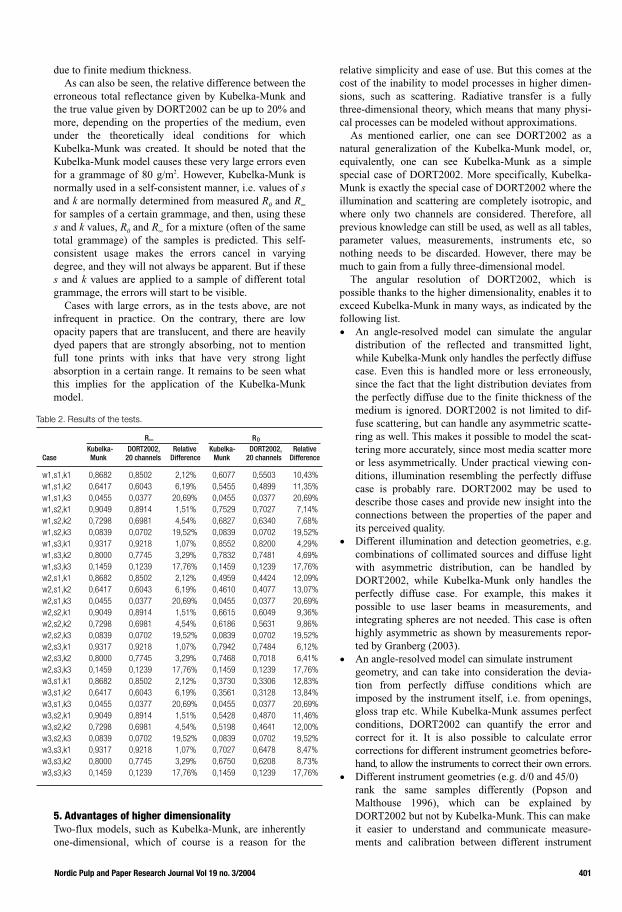
401Nordic Pulp and Paper Research Journal Vol 19 no. 3/2004
due to finite medium thickness.As can also be seen, the relative difference between the
erroneous total reflectance given by Kubelka-Munk andthe true value given by DORT2002 can be up to 20% andmore, depending on the properties of the medium, evenunder the theoretically ideal conditions for whichKubelka-Munk was created. It should be noted that theKubelka-Munk model causes these very large errors evenfor a grammage of 80 g/m2. However, Kubelka-Munk isnormally used in a self-consistent manner, i.e. values of sand k are normally determined from measured R0 and R∞for samples of a certain grammage, and then, using theses and k values, R0 and R∞ for a mixture (often of the sametotal grammage) of the samples is predicted. This self-consistent usage makes the errors cancel in varyingdegree, and they will not always be apparent. But if theses and k values are applied to a sample of different totalgrammage, the errors will start to be visible.
Cases with large errors, as in the tests above, are notinfrequent in practice. On the contrary, there are lowopacity papers that are translucent, and there are heavilydyed papers that are strongly absorbing, not to mentionfull tone prints with inks that have very strong lightabsorption in a certain range. It remains to be seen whatthis implies for the application of the Kubelka-Munkmodel.
5. Advantages of higher dimensionality Two-flux models, such as Kubelka-Munk, are inherentlyone-dimensional, which of course is a reason for the
relative simplicity and ease of use. But this comes at thecost of the inability to model processes in higher dimen-sions, such as scattering. Radiative transfer is a fullythree-dimensional theory, which means that many physi-cal processes can be modeled without approximations.
As mentioned earlier, one can see DORT2002 as anatural generalization of the Kubelka-Munk model, or,equivalently, one can see Kubelka-Munk as a simplespecial case of DORT2002. More specifically, Kubelka-Munk is exactly the special case of DORT2002 where theillumination and scattering are completely isotropic, andwhere only two channels are considered. Therefore, allprevious knowledge can still be used, as well as all tables,parameter values, measurements, instruments etc, sonothing needs to be discarded. However, there may bemuch to gain from a fully three-dimensional model.
The angular resolution of DORT2002, which ispossible thanks to the higher dimensionality, enables it toexceed Kubelka-Munk in many ways, as indicated by thefollowing list.
• An angle-resolved model can simulate the angulardistribution of the reflected and transmitted light,while Kubelka-Munk only handles the perfectly diffusecase. Even this is handled more or less erroneously,since the fact that the light distribution deviates fromthe perfectly diffuse due to the finite thickness of themedium is ignored. DORT2002 is not limited to dif-fuse scattering, but can handle any asymmetric scatte-ring as well. This makes it possible to model the scat-tering more accurately, since most media scatter moreor less asymmetrically. Under practical viewing con-ditions, illumination resembling the perfectly diffusecase is probably rare. DORT2002 may be used todescribe those cases and provide new insight into theconnections between the properties of the paper andits perceived quality.
• Different illumination and detection geometries, e.g.combinations of collimated sources and diffuse lightwith asymmetric distribution, can be handled byDORT2002, while Kubelka-Munk only handles theperfectly diffuse case. For example, this makes it possible to use laser beams in measurements, and integrating spheres are not needed. This case is oftenhighly asymmetric as shown by measurements repor-ted by Granberg (2003).
• An angle-resolved model can simulate instrumentgeometry, and can take into consideration the devia-tion from perfectly diffuse conditions which areimposed by the instrument itself, i.e. from openings,gloss trap etc. While Kubelka-Munk assumes perfectconditions, DORT2002 can quantify the error andcorrect for it. It is also possible to calculate error corrections for different instrument geometries before-hand, to allow the instruments to correct their own errors.
• Different instrument geometries (e.g. d/0 and 45/0)rank the same samples differently (Popson andMalthouse 1996), which can be explained by DORT2002 but not by Kubelka-Munk. This can makeit easier to understand and communicate measure-ments and calibration between different instrument
R∞ R0
Kubelka- DORT2002, Relative Kubelka- DORT2002, RelativeCase Munk 20 channels Difference Munk 20 channels Difference
w1,s1,k1 0,8682 0,8502 2,12% 0,6077 0,5503 10,43%w1,s1,k2 0,6417 0,6043 6,19% 0,5455 0,4899 11,35%w1,s1,k3 0,0455 0,0377 20,69% 0,0455 0,0377 20,69%w1,s2,k1 0,9049 0,8914 1,51% 0,7529 0,7027 7,14%w1,s2,k2 0,7298 0,6981 4,54% 0,6827 0,6340 7,68%w1,s2,k3 0,0839 0,0702 19,52% 0,0839 0,0702 19,52%w1,s3,k1 0,9317 0,9218 1,07% 0,8552 0,8200 4,29%w1,s3,k2 0,8000 0,7745 3,29% 0,7832 0,7481 4,69%w1,s3,k3 0,1459 0,1239 17,76% 0,1459 0,1239 17,76%w2,s1,k1 0,8682 0,8502 2,12% 0,4959 0,4424 12,09%w2,s1,k2 0,6417 0,6043 6,19% 0,4610 0,4077 13,07%w2,s1,k3 0,0455 0,0377 20,69% 0,0455 0,0377 20,69%w2,s2,k1 0,9049 0,8914 1,51% 0,6615 0,6049 9,36%w2,s2,k2 0,7298 0,6981 4,54% 0,6186 0,5631 9,86%w2,s2,k3 0,0839 0,0702 19,52% 0,0839 0,0702 19,52%w2,s3,k1 0,9317 0,9218 1,07% 0,7942 0,7484 6,12%w2,s3,k2 0,8000 0,7745 3,29% 0,7468 0,7018 6,41%w2,s3,k3 0,1459 0,1239 17,76% 0,1459 0,1239 17,76%w3,s1,k1 0,8682 0,8502 2,12% 0,3730 0,3306 12,83%w3,s1,k2 0,6417 0,6043 6,19% 0,3561 0,3128 13,84%w3,s1,k3 0,0455 0,0377 20,69% 0,0455 0,0377 20,69%w3,s2,k1 0,9049 0,8914 1,51% 0,5428 0,4870 11,46%w3,s2,k2 0,7298 0,6981 4,54% 0,5198 0,4641 12,00%w3,s2,k3 0,0839 0,0702 19,52% 0,0839 0,0702 19,52%w3,s3,k1 0,9317 0,9218 1,07% 0,7027 0,6478 8,47%w3,s3,k2 0,8000 0,7745 3,29% 0,6750 0,6208 8,73%w3,s3,k3 0,1459 0,1239 17,76% 0,1459 0,1239 17,76%
Table 2. Results of the tests.
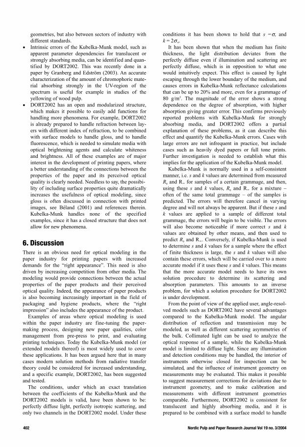
402 Nordic Pulp and Paper Research Journal Vol 19 no. 3/2004
geometries, but also between sectors of industry withdifferent standards.
• Intrinsic errors of the Kubelka-Munk model, such asapparent parameter dependencies for translucent or strongly absorbing media, can be identified and quan-tified by DORT2002. This was recently done in apaper by Granberg and Edström (2003). An accuratecharacterization of the amount of chromophoric mate-rial absorbing strongly in the UV-region of the spectrum is useful for example in studies of the yellowing of wood pulp.
• DORT2002 has an open and modularized structure,which makes it possible to easily add functions forhandling more phenomena. For example, DORT2002 is already prepared to handle refraction between lay-ers with different index of refraction, to be combinedwith surface models to handle gloss, and to handlefluorescence, which is needed to simulate media with optical brightening agents and calculate whitenessand brightness. All of these examples are of majorinterest in the development of printing papers, where a better understanding of the connections between theproperties of the paper and its perceived optical quality is clearly needed. Needless to say, the possibi-lity of including surface properties quite dramaticallyincreases the usefulness of optical modeling, since gloss is often discussed in connection with printed images, see Béland (2001) and references therein.Kubelka-Munk handles none of the specified examples, since it has a closed structure that does not allow for new phenomena.
6. Discussion There is an obvious need for optical modeling in thepaper industry for printing papers with increaseddemands for the “right appearance”. This need is alsodriven by increasing competition from other media. Themodeling would provide connections between the actualproperties of the paper products and their perceivedoptical quality. Indeed, the appearance of paper productsis also becoming increasingly important in the field ofpackaging and hygiene products, where the “rightimpression” also includes the appearance of the product.
Examples of areas where optical modeling is usedwithin the paper industry are fine-tuning the paper-making process, designing new paper qualities, colormanagement from pre-press to print, and evaluatingprinting techniques. Today the Kubelka-Munk model (orextended models thereof) is most widely used to coverthese applications. It has been argued here that in manycases modern solution methods from radiative transfertheory could be considered for increased understanding,and a specific example, DORT2002, has been suggestedand tested.
The conditions, under which an exact translationbetween the coefficients of the Kubelka-Munk and theDORT2002 models is valid, have been shown to be:perfectly diffuse light, perfectly isotropic scattering, andonly two channels in the DORT2002 model. Under these
conditions it has been shown to hold that s =σs andk = 2σ a.
It has been shown that when the medium has finitethickness, the light distribution deviates from theperfectly diffuse even if illumination and scattering areperfectly diffuse, which is in opposition to what onewould intuitively expect. This effect is caused by lightescaping through the lower boundary of the medium, andcauses errors in Kubelka-Munk reflectance calculationsthat can be up to 20% and more, even for a grammage of80 g/m2. The magnitude of the error shows a strongdependence on the degree of absorption, with higherabsorption giving greater error. This confirms previouslyreported problems with Kubelka-Munk for stronglyabsorbing media, and DORT2002 offers a partialexplanation of these problems, as it can describe thiseffect and quantify the Kubelka-Munk errors. Cases withlarge errors are not infrequent in practice, but includecases such as heavily dyed papers or full tone prints.Further investigation is needed to establish what thisimplies for the application of the Kubelka-Munk model.
Kubelka-Munk is normally used in a self-consistentmanner, i.e. s and k values are determined from measuredR0 and R∞ for samples of a certain grammage, and then,using these s and k values, R0 and R∞ for a mixture –often of the same total grammage – of the samples ispredicted. The errors will therefore cancel in varyingdegree and will not always be apparent. But if these s andk values are applied to a sample of different totalgrammage, the errors will begin to be visible. The errorswill also become noticeable if more correct s and kvalues are obtained by other means, and then used topredict R0 and R∞. Conversely, if Kubelka-Munk is usedto determine s and k values for a sample where the effectof finite thickness is large, the s and k values will alsocontain these errors, which will be carried over to a moreaccurate model if it uses these s and k values. This meansthat the more accurate model needs to have its ownsolution procedure to determine its scattering andabsorption parameters. This amounts to an inverseproblem, for which a solution procedure for DORT2002is under development.
From the point of view of the applied user, angle-resol-ved models such as DORT2002 have several advantagescompared to the Kubelka-Munk model. The angulardistribution of reflection and transmission may bemodeled, as well as different scattering asymmetries ofthe bulk. Collimated light can be used to analyze theoptical response of a sample, while the Kubelka-Munkmodel is limited to diffuse light. Since any illuminationand detection conditions may be handled, the interior ofinstruments otherwise closed for inspection can besimulated, and the influence of instrument geometry onmeasurements may be evaluated. This makes it possibleto suggest measurement corrections for deviations due toinstrument geometry, and to make calibration andmeasurements with different instrument geometriescomparable. Furthermore, DORT2002 is consistent fortranslucent and highly absorbing media, and it isprepared to be combined with a surface model to handle
403Nordic Pulp and Paper Research Journal Vol 19 no. 3/2004
gloss. It is also prepared for a future implementation offluorescence, which will allow the effect of OBA (opticalbrightening agents) in paper and print to be modeled.This opens the field for finding new connections betweenthe properties of paper and its perceived optical quality.The whiteness and brightness of paper cannot bedesigned with the Kubelka-Munk model sincefluorescence phenomena are not explicitly included.
These improvements are important for a number ofreasons. Paper may be translucent, glossy and stronglyabsorbing, e.g. low opacity paper, calendered paper, andheavily dyed paper or full tone prints. The standardizedmeasurement geometries (d/0 and 45/0) for reflectancefactors such as brightness of paper may give differentrankings, which cannot be explained by the Kubelka-Munk model, but is readily given by DORT2002.Moreover, there is experimental evidence that thereflection and transmission of paper and print deviatesfrom the Kubelka-Munk model description (Granberg(2003)), which can be interpreted more accurately byDORT2002.
As mentioned earlier, since Kubelka-Munk is a simplespecial case of DORT2002, all previous knowledge suchas tables, parameter values, measurements etc can still beused, so nothing needs to be discarded. On the contrary, itprovides a strong foundation for future work with bothmodels. A solution procedure for the inverse problem ofDORT2002 is required to complete the picture, butDORT2002 may well be considered at present forincreased understanding in cases where the level of accu-racy of Kubelka-Munk reflectance calculations is notacceptable.
Acknowledgements
The author wishes to thank professor Tetsu Uesaka for valuable comments on themanuscript and for discussions on applied paper optics. Thanks also go to DrMats Rundlöf and Dr Hjalmar Granberg. This work was financially supported bythe Swedish printing research program T2F, “TryckTeknisk Forskning”, which isgratefully acknowledged.
Literature
van den Akker, J. A. (1949): Scattering and Absorption of Light in Paper andOther Diffusing Media, TAPPI 32, pp 498-501.van den Akker, J. A. (1966): Discussion on Relationships Between Mechanicaland Optical Properties of Paper Affected by Web Consolidation, Trans. Symp.Consolidation Paper Web, Tech. Sect. Brit. Paper Board Maker’s Assoc., London,UK, pp 948-950.
van den Akker, J. A. (1968): Theory of Some of the Discrepancies Observed inApplication of the Kubelka-Munk Equations to Particulate Systems, in “ModernAspects of Reflectance Spectroscopy”, W. W. Wendlandt, Ed., Plenum Press, NewYork, NY, USA, pp 27-46.Béland, M.-C. (2001): Gloss Variation of Printed Paper: Relationship BetweenTopography and Light Scattering, Doctoral Thesis, Royal Institute of Technology,Stockholm.Chandrasekhar, S. (1944a): On the Radiative Equilibrium of a StellarAtmosphere, Astrophys. J. 99, pp 180-190.Chandrasekhar, S. (1944b): On the Radiative Equilibrium of a Stellar AtmosphereII, Astrophys. J. 100, pp 76-86.Chandrasekhar, S. (1960): Radiative Transfer, Dover, New York.Edström, P. (2003): A Fast and Stable Solution Method for the Radiative TransferProblem, to appear in SIAM Rev.Edström, P. (2004): Numerical Performance of the DORT2002 Radiative TransferSolution Method, submitted to Appl. Numer. Math.Foote, W. J. (1939): An Investigation of the Fundamental Scattering andAbsorption Coefficients of Dyed Handsheets, Paper Trade J. 109, pp 333-340.Granberg, H. (2003): Optical Response from Paper: Angle-dependent LightScattering Measurements, Modelling and Analysis, Doctoral Thesis, Royal Instituteof Technology, Stockholm.Granberg, H. and Edström, P. (2003): Quantification of the Intrinsic Error of theKubelka-Munk Model Caused by Strong Light Absorption, J. Pulp Paper Sci.29(11), pp 386-390.Koukoulas, A. A. and Jordan, B. D. (1997): Effect of Strong Absorption on theKubelka-Munk Scattering Coefficient, J. Pulp Paper Sci. 23(5), pp 224-232.Kubelka, P. and Munk, F. (1931): Ein Beitrag zur Optik der Farbanstriche, Z.Tech. Phys. 11a, pp 593-601.Kubelka, P. (1948): New Contributions to the Optics of Intensely Light-ScatteringMaterials. Part I, J. Opt. Soc. Am. 38, pp 448-457.Kubelka, P. (1954): New Contributions to the Optics of Intensely Light-ScatteringMaterials. Part II, J. Opt. Soc. Am. 44, pp 330-335.Moldenius, S. (1983): Light Absorption Coefficient Spectra of Hydrogen PeroxideBleached Mechanical Pulp, Paperi Puu 65(11), pp 747-756.Nordman, L., Aaltonen, P. and Makkonen, T. (1966): Relationships BetweenMechanical and Optical Properties of Paper Affected by Web Consolidation, Trans.Symp. Consolidation Paper Web, Tech. Sect. Brit. Paper Board Maker’s Assoc.,London, UK, pp 909-927.Pauler, N. (2002): Paper Optics, Lorentzen & Wettre, Kista, Sweden.Popson, J. S. and Malthouse, D. D. (1996): Measurement and Control of theOptical Properties of Paper, 2nd edition, Technidyne Corporation, USA.Rundlöf, M. and Bristow, J. A. (1997): A Note Concerning the InteractionBetween Light Scattering and Light Absorption in the Application of the Kubelka-Munk Equations, J. Pulp Paper Sci. 23(5), pp 220-223.Schuster, A. (1905): Radiation Trough a Foggy Atmosphere, Astrophys. J. 21, pp1-22. (Reprinted in Selected Papers on the Transfer of Radiation, Dover, NewYork, 1966. Edited Menzel, D. H.) Wick, G. C. (1943): Über ebene Diffusionsprobleme, Z. Phys. 120, pp 702-718.
Manuscript received April 16, 2004Accepted June, 2004


IV

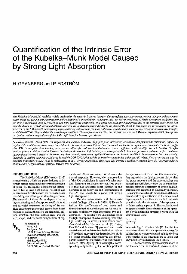
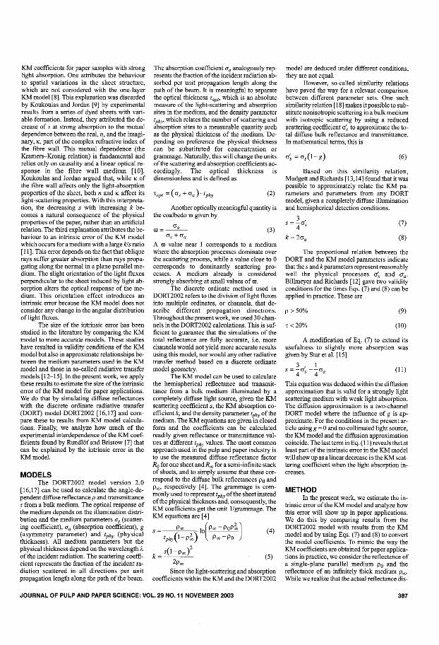
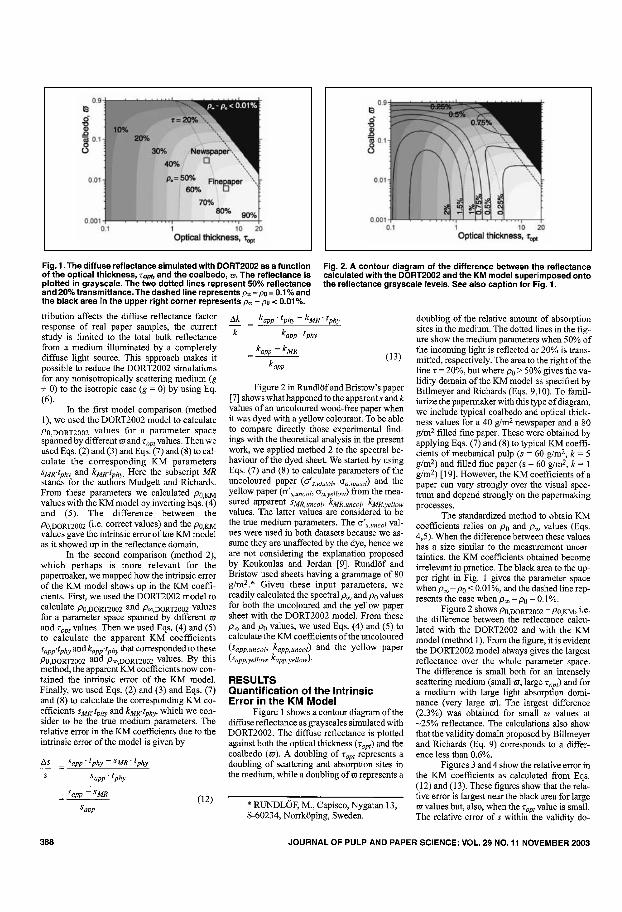
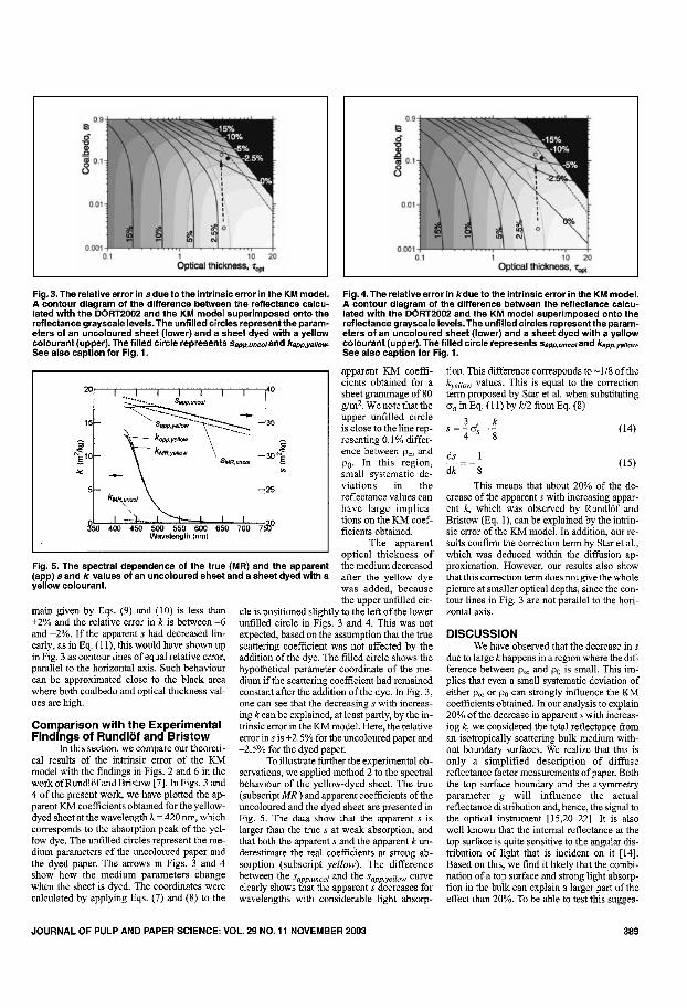


V

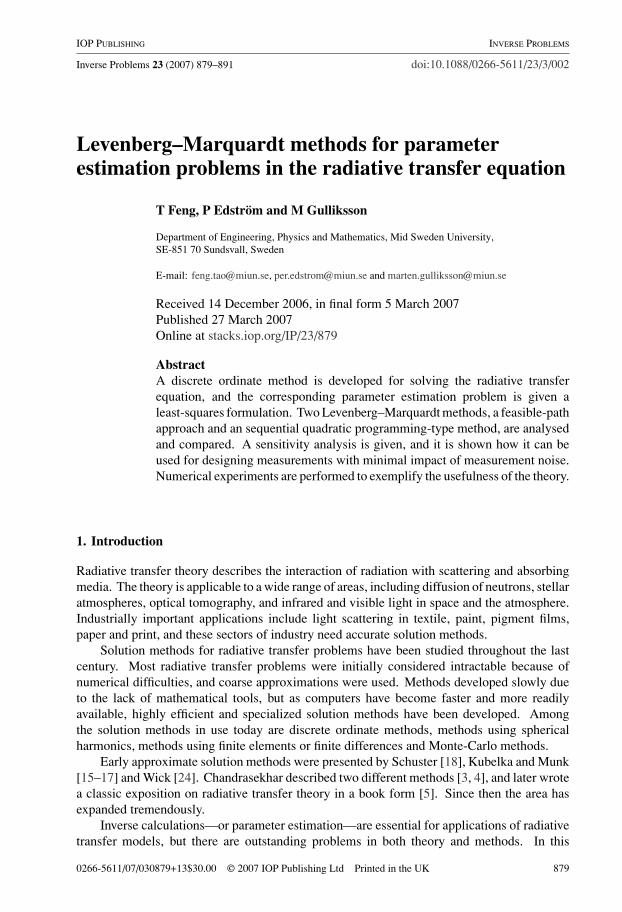
IOP PUBLISHING INVERSE PROBLEMS
Inverse Problems 23 (2007) 879–891 doi:10.1088/0266-5611/23/3/002
Levenberg–Marquardt methods for parameterestimation problems in the radiative transfer equation
T Feng, P Edstrom and M Gulliksson
Department of Engineering, Physics and Mathematics, Mid Sweden University,SE-851 70 Sundsvall, Sweden
E-mail: [email protected], [email protected] and [email protected]
Received 14 December 2006, in final form 5 March 2007Published 27 March 2007Online at stacks.iop.org/IP/23/879
AbstractA discrete ordinate method is developed for solving the radiative transferequation, and the corresponding parameter estimation problem is given aleast-squares formulation. Two Levenberg–Marquardt methods, a feasible-pathapproach and an sequential quadratic programming-type method, are analysedand compared. A sensitivity analysis is given, and it is shown how it can beused for designing measurements with minimal impact of measurement noise.Numerical experiments are performed to exemplify the usefulness of the theory.
1. Introduction
Radiative transfer theory describes the interaction of radiation with scattering and absorbingmedia. The theory is applicable to a wide range of areas, including diffusion of neutrons, stellaratmospheres, optical tomography, and infrared and visible light in space and the atmosphere.Industrially important applications include light scattering in textile, paint, pigment films,paper and print, and these sectors of industry need accurate solution methods.
Solution methods for radiative transfer problems have been studied throughout the lastcentury. Most radiative transfer problems were initially considered intractable because ofnumerical difficulties, and coarse approximations were used. Methods developed slowly dueto the lack of mathematical tools, but as computers have become faster and more readilyavailable, highly efficient and specialized solution methods have been developed. Amongthe solution methods in use today are discrete ordinate methods, methods using sphericalharmonics, methods using finite elements or finite differences and Monte-Carlo methods.
Early approximate solution methods were presented by Schuster [18], Kubelka and Munk[15–17] and Wick [24]. Chandrasekhar described two different methods [3, 4], and later wrotea classic exposition on radiative transfer theory in a book form [5]. Since then the area hasexpanded tremendously.
Inverse calculations—or parameter estimation—are essential for applications of radiativetransfer models, but there are outstanding problems in both theory and methods. In this
0266-5611/07/030879+13$30.00 © 2007 IOP Publishing Ltd Printed in the UK 879
880 T Feng et al
paper, the parameter estimation problem is formulated as an optimization problem, and theaim is to recover some unknown parameters in the mathematical model. The majority ofparameter estimation problems are ill-posed due to the presence of data noise. Therefore,regularization methods have to be used to obtain stable approximations of the solution, such asthe classical Tikhonov regularization [7]. In this paper, an iterative regularization method, theLevenberg–Marquardt method, is applied, where the iteration follows a feasible path definedby the underlying state equation. Moreover, an iterative regularization method based on theidea of sequential quadratic programming is discussed. An important difference between thesequential quadratic programming (SQP)-type Levenberg–Marquardt method and the feasible-path approach is that the underlying state equation is interpreted as a constraint in the productspace of state and parameter variables, and is approximated by a linearized version in eachiteration step.
In this work, the unknown parameters are estimated with some pointwise measurements.In order to study the influence of perturbations in the measurements on the parameter solution,a quantity is derived based on the sensitivity analysis. This quantity can help to interpret thefinal results, and to indicate better locations for the measurement points.
Calculating material parameters from reflectance measurements is straightforward in thesimpler Kubelka–Munk method, but is an outstanding problem in general radiative transferproblems. Estimating the scattering and absorption parameters with a radiative transfer modelwould be valuable for the paper industry since it could increase the accuracy, it could explain thedifferent ranking of paper samples and it could resolve problems regarding ink characterization.Another important benefit would be the possibility of exchanging data between the paper andthe graphical industries. This is currently not possible due to different instrument geometries,while the Kubelka–Munk parameters are geometry dependent. Estimating the asymmetryfactor as well would increase the value further since it could give a better understandingof the paper medium, and it could also facilitate the design of new phenomena in papermaterials. Finally, the sensitivity analysis points out which parameters are sensitive to whatmeasurements, which shows the kind of accuracy that can be expected from the estimations,but it also helps to design new measurements with minimal impact of measurement noise.
In section 2, we formulate the forward problem and describe our discrete ordinate solutionmethods. The parameter estimation problem is formulated and discussed in section 3. Insection 4, Levenberg–Marquardt methods are investigated and compared in some detail, andin section 5, a sensitivity analysis is performed. Numerical experiments are presented insection 6, and some comments are made in section 7.
2. Forward problem
This section gives a short introduction to the forward radiative transfer problem includingassumptions, a formulation and some discrete ordinate solution methods.
To describe radiation in a turbid medium, specular reflection at surfaces must be taken intoconsideration, as well as transmission, absorption and multiple scattering inside the medium.The problem is often studied in a plane-parallel geometry, where the horizontal extension ofthe medium is assumed to be large enough to give no boundary effects at the sides. At thetop and bottom boundary surfaces, boundary conditions are assumed to be time and spaceindependent. The radiation is assumed to be monochromatic, and the scattering is assumed tobe conservative, i.e. without change in frequency between incoming and outgoing radiation.The medium is treated as a continuum of scattering and absorption sites. Polarization effectsare ignored, and what is left is then a scalar intensity, which is the variable to solve for.
Levenberg–Marquardt methods for parameter estimation problems 881
Edstrom [6] states the equation of radiative transfer as
udI (τ, u, ϕ)
dτ= I (τ, u, ϕ) − 1
4π
σs
σs + σa
∫ 2π
0
∫ 1
−1p(u′, ϕ′; u, ϕ)I (τ, u′, ϕ′) du′ dϕ′. (1)
The unknown intensity I at optical depth τ is considered as non-interacting beams of radiationin all directions. The scattering and absorption coefficients of the medium are denoted byσs and σa , and the phase function p specifies the probability distribution of scattering fromincident direction (u′, ϕ′) to direction (u, ϕ), where u is cosine of polar angle and ϕ is azimuthalangle. The shape of the phase function is controlled by a parameter called the asymmetryfactor, g, ranging from complete forward scattering (g = 1) over isotropic scattering (g = 0)
to complete backward scattering (g = −1). Different phase functions have been proposed tophysically describe different types of scattering. This paper considers the Henyey–Greenstein[13] phase function. It should not be seen as a real phase function, but is a one-parameteranalytical approximation of widespread use. It is given by
p(cos �) = 1 − g2
(1 + g2 − 2g cos �)3/2, (2)
where � is the scattering angle. It is thus evident that the Henyey–Greenstein phase functionis dependent on the scattering angle � only, and not on the specific directions of incident andscattered radiation.
Discrete ordinate solution methods are among the most used and most accurate solutionmethods today. Stamnes and co-workers [20, 21] presented in a series of papers the successivedevelopment of a stable discrete ordinate algorithm and provided a software package, DISORT.Thomas and Stamnes [22] also wrote a textbook on radiative transfer in the atmosphere. In arecent paper, Edstrom [6] presented a systematic review of the stability-enhancing and speed-increasing steps used in modern discrete ordinate radiative transfer algorithms. Edstrom alsopresented the solution method DORT2002, which is adapted to light scattering simulations inpaper and print, but which is also designed for methodical numerical experiments. DORT2002uses Fourier analysis on the azimuthal angle to turn the integro-differential equation (1) intoa number of uncoupled equations, one for each Fourier component of the unknown intensity,which are then discretized using numerical quadrature. This yields a system of first-orderlinear differential equations for each Fourier component, and the natural solution proceduregives an eigenvalue problem.
In this paper, discrete ordinate methods are still used. However, the method used herediffers from DORT2002. First, the integral is discretized with a Gauss quadrature, and theresulting ordinary differential equation is solved using a backward Euler finite differencemethod (cf [19]). The reason for not using DORT2002, although it could equally well havebeen used for the forward problem (1), is that it cannot solve the similar equations (37) and(38). Those equations give the derivative information needed in the parameter estimationproblem. It involves too much work to adapt the large and versatile DORT2002 code for thispurpose in the current study, and it is believed that this strategy can be implemented equallyefficiently.
By using Gauss quadrature for the integrals, a semi-discrete formulation of the radiativetransfer equation (1) is given by
uk
dI (τ, uk, ϕk)
dτ= I (τ, uk, ϕk) − 1
4π
σs
σs + σa
×M∑l=1
wlp(u′l , ϕ
′l; uk, ϕk)I (τ, u′
l , ϕ′l ), k = 1, 2, . . . , M, (3)
882 T Feng et al
where (u′l , ϕ
′l ) denotes the required quadrature point and wl the corresponding weights (see
[10]). For simplicity of expression, we let
Ik = I (τ, uk, ϕk)
and
φk(τ ) =M∑l=1
wlp(u′l , ϕ
′l; uk, ϕk)I (τ, u′
l , ϕ′l ).
We then let Ik and φk represent the respective function’s values at a discrete set of points,
τj = τ0 + jh, j = 0, 1, . . . , N,
where h is the grid spacing. We use subscript j to denote the approximate value of any functionat the grid point τj . By using a backward Euler finite difference method in (3), a fully discreteapproximation of the radiative transfer equation (1) can be written as
uk
Ik,j+1 − Ik,j
h= 1
2(Ik,j+1 + Ik,j ) − 1
8π
σs
σs + σa
(φk,j+1 + φk,j ). (4)
An iterative method, the source iteration method [19], is employed to solve the system(4). Given an initial guess of the intensity, I 0
k,j , we compute in each iteration the termφi
k,j+1 + φik,j , i = 0, 1, 2 . . . . Then, by using algorithm 1 introduced in [19] as sweeping
procedure, the new values of the intensity, I ik,j , i = 1, 2 . . . , can be obtained. In the sweeping
procedure, we compute the intensity with uk > 0 and the intensity with uk < 0 separately,combining with the boundary conditions. Our algorithm terminates with the same stoppingrule as algorithm 2 in [19].
3. The parameter estimation problem
In the radiative transfer equation, there are three obvious scalar parameters to estimate, thescattering coefficient σs , the absorption coefficient σa and the asymmetry factor g. In thissection, an optimization problem is formulated in order to estimate these parameters by usingcertain measured quantities.
We denote q = (σs, σa, g)T and let q ∈ Qad , where
Qad ≡ {(σs, σa, g)T : σs > 0, σa > 0, 1 > g > −1}is the admissible parameter set. To simplify the analysis, the equation of radiative transfer iswritten as
e(I, q) = udI (τ, u, ϕ)
dτ− I (τ, u, ϕ)
+1
4π
σs
σs + σa
∫ 2π
0
∫ 1
−1p(u′, ϕ′; u, ϕ)I (τ, u′, ϕ′) du′ dϕ′ = 0, (5)
where I ⊂ U and e : U × R3 → Y . Here, U and Y are appropriate Hilbert spaces (see [14]for instance), and we assume that e is continuously Frechet differentiable. Suppose we havean observation z = CI and C : U → Z is a bounded linear operator, where Z is a Hilbertspace. In our numerical example, the pointwise measurements of intensity I are obtained andZ = Rnm , where nm is the number of the measurement points. In practice, one has to dealwith the noise data zδ . To recover the unknown parameters, a least-squares formulation isemployed, i.e., we solve the optimization problem
min(I,q)∈U×Qad
J (I, q) = 12‖CI − zδ‖2
Z, (6)
Levenberg–Marquardt methods for parameter estimation problems 883
subject to (5). Usually, the parameter estimation problem is an ill-posed problem. Therefore,regularization methods have to be used in order to obtain stable approximations of the solutionin the presence of data noise. One classical approach is the Tikhonov-type regularization(see [7]).
Recently, the application of iterative regularization methods has been investigated (see[1, 2, 11, 12, 23]), and they work very well on several parameter estimation problems.Inspired by these earlier works, we studied the Levenberg–Marquardt method for our parameterestimation problem.
4. The Levenberg–Marquardt method
4.1. Levenberg–Marquardt method on feasible paths
Hanke studied iterative regularization methods based on a feasible-path approach [11, 12],where the state equation is eliminated and the resulting parameter-to-output map is theconcatenation of the parameter-to-state map q → I and the observation operator C. In orderto derive the parameter-to-state map, we firstly state the weak form of the radiative transferequation as
e(I, q)(φ) = 0, ∀φ ∈ U, (7)
where
e(I, q)(φ) =∫ τd
0
∫ 2π
0
∫ 1
−1u
dI (τ, u, ϕ)
dτφ(τ, u, ϕ) du dϕ dτ
−∫ τd
0
∫ 2π
0
∫ 1
−1I (τ, u, ϕ)φ(τ, u, ϕ) du dϕ dτ
+1
4π
σs
σs + σa
∫ τd
0
∫ 2π
0
∫ 1
−1
∫ 2π
0
∫ 1
−1p(u′, ϕ′; u, ϕ)I (τ, u′, ϕ′)
×φ(τ, u, ϕ) du′ dϕ′ du dϕ dτ,
and τd is the optical depth of the sample. It is clear that the functional e(I, q)(φ) is linear withrespect to both I and φ. We denote the partial derivatives of the weak form by e′
I (·, ·)(·, ·)and e′
q(·, ·)(·, ·) etc. Under certain conditions, it can be proved (cf e.g. [14]) that there existsa γ > 0 such that
e(I, q)(I ) � γ ‖I‖2U . (8)
Thereafter, we can derive the following proposition.
Proposition 4.1. In a neighbourhood of the solution to the minimization problem (6), thederivative e′
I (I, q)(h, h) is coercive, i.e. there exists a positive constant γ such that
e′I (I, q)(h, h) � γ ‖h‖2
U , ∀h ∈ U. (9)
Proof. By the weak form of the radiative transfer equation, it is easy to see that e(·, ·)(·) islinear with respect to the first argument. Thus, we have
e(h, q)(h) = e′I (I, q)(h, h).
By (8),
e′I (I, q)(h, h) = e(h, q)(h) � γ ‖h‖2
U . �
This result implies that the operator e′I (I, q) is an isomorphism [8]. Hence, by the implicit
function theorem, it can be concluded that problem (5) has a unique solution I = S(q) in Q0,
884 T Feng et al
where Q0 is a neighbourhood of the solution to (5). Here, S is called a parameter-to-state map.We can also define a nonlinear operator F ≡ CS : Q → Z and reformulate the parameterestimation problem (6) as
minq∈Q
J (q) = 12‖F(q) − zδ‖2
Z. (10)
By using Levenberg–Marquardt methods, the iterates are computed from
[F ′(qk)∗F ′(qk) + βkId](qk+1 − qk) = −F ′(qk)∗(F (qk) − zδ), (11)
where Id denotes the identity matrix and the parameter (βk)k∈N is a bounded sequence ofpositive real numbers. It is not difficult to see that (11) is equivalent to the minimizationproblem
minq∈Q
‖F(qk) − zδ + F ′(qk)(q − qk)‖2Z + βk‖q − qk‖2
Q. (12)
Assume that the nonlinear condition
‖F (q) − F(q) − F ′(q)(q − q)‖Z � c‖q − q‖Q‖F (q) − F(q)‖Z (13)
is fulfilled for all q, q in some neighbourhood of a solution, where c is a positive constant. Byusing the generalized discrepancy principle, it has been proved (see [12]) that the Levenberg–Marquardt method is locally convergent in the presence of noise.
From (11), it is easy to see that the main effort is to compute F ′(q). To this end, we usethe chain rule and the linearity of the observation operator to obtain
F ′(q) = CS ′(q). (14)
We differentiate (5) and obtain
e′I (S(q), q)S ′(q) + e′
q(S(q), q) = 0, (15)
where
e′I (I, q)δI = u
dδI
dτ− δI +
1
4π
σs
σs + σa
∫ 2π
0
∫ 1
−1pδI du′ dϕ′, (16)
e′q(I, q)δq = e′
σs(I, q)δσs + e′
σa(I, q)δσa + e′
g(I, q)δg, (17)
with
e′σs
(I, q)δσs = σaδσs
4π(σs + σa)2
∫ 2π
0
∫ 1
−1pI du′ dϕ′, (18)
e′σa
(I, q)δσa = − σsδσa
4π(σs + σa)2
∫ 2π
0
∫ 1
−1pI du′ dϕ′, (19)
e′g(I, q)δg = 1
4π
σs
σs + σa
∫ 2π
0
∫ 1
−1p′
gδgI du′ dϕ′. (20)
Since the operator e′I (I, q), as shown above, is an isomorphism, equation (15) can be uniquely
solved for S ′(q), which is needed for the evaluation of F ′(q) in (14). The main algorithm canbe summarized as follows.
Algorithm 4.2. Set convergence tolerance tol and maximum iteration number Maxiter;Choose initial values q0 by a priori information and β0 > 0; Set k := 0;while ‖∇J (qk)‖ > tol and k < Maxiter
Solve the equation of radiative transfer (5) and obtain I k;
Levenberg–Marquardt methods for parameter estimation problems 885
Solve (15) and compute F ′(qk) by (14);Compute qk+1 by solving (11);if J (qk) > J (qk+1)
βk+1 := 0.1βk;endwhile J (qk) < J (qk+1)
βk+1 := 10βk , compute qk+1 by solving (11);end
k := k + 1;end
In the numerical experiment presented in section 6, we let β0 = 10−5, and the parameterβk is reduced or expanded by a factor of 10. However, it should be mentioned that theparameter βk can be updated in another way (see [9]), and that the update rule should dependon the noise in the measurement data. Another strategy for choosing the parameter βk hasbeen studied for nonlinear ill-posed inverse problems [12], where the author made tests tocompare their methods to the standard methods. It was concluded that both methods couldgenerate comparable results. Thereafter, Wang and Yuan (see [23]) studied the convergenceand regularity of the standard trust region methods for nonlinear ill-posed inverse problems.It turned out that the standard trust region methods are indeed a regularization, and theconvergence result was also proved. In the presence of data noise, an additional stopping rulefor the iteration can be introduced as in [12] according to the discrepancy principle.
4.2. SQP-type Levenberg–Marquardt method
Very recently, an SQP-type Levenberg–Marquardt method was investigated (see [1, 2]), wherethe underlying state equation was interpreted as a constraint in the product space of state andparameter variables, and approximated by a linearized version in each iteration step. Bothstate and parameter variables can be computed by solving the Karush–Kuhn–Tucker (KKT)system.
We linearize the objective and constraint function in (6) and add a regularization termR(q) = ‖δq‖2
Q,
min(δI,δq)∈U×Q
{1
2‖CI + CδI − zδ‖2
Z +β
2‖δq‖2
Q
}, (21)
subject to the linear constraint
e(I, q) + e′I (I, q)δI + e′
q(I, q)δq = 0. (22)
In the k′th iteration, the regularization parameter β = βk , and the Lagrangian of the problems(21) and (22) can be written as
L(δI, δq, δλ) = 1
2‖CI + CδI − zδ‖2
Z +β
2‖δq‖2
Q + 〈(λ + δλ), (e(I, q)
+ e′I (I, q)δI + e′
q(I, q)δq)〉.The solution now satisfies the optimality condition
L′(δI, δq, δλ) = 0, (23)
where (δI, δq, δλ) are the new search directions.
886 T Feng et al
This gives the KKT system⎛⎝C∗C 0 K∗
0 βId L∗
K L 0
⎞⎠
⎛⎝δI
δq
δλ
⎞⎠ =
⎛⎝C∗(zδ − CI) − (e′
I (I, q))∗λ−(e′
q(I, q))∗λe(I, q)
⎞⎠ =
⎛⎝RI
Rq
Rλ
⎞⎠ ,
where we define the operators K and L as
KδI = e′I (I, q)δI, Lδq = e′
q(I, q)δq, (24)
and we denote the adjoint operators of K and L by K∗ and L∗. Here, the operator L is givenexplicitly by relations (18)–(20). Since g is not estimated in the numerical experiments in thispaper, δg is zero, and e′
g(I, q)δg is not needed.
4.3. Relationship between these two Levenberg–Marquardt methods
In order to investigate the relationship between these two Levenberg–Marquadt methods, wecompute the Schur complement of the KKT system with respect to q, and the equation for δq
has the form{βId − [0, L∗]
[0 K−1
K−∗ −K−∗C∗CK−1
] [0L
]}δq
= Rq − [0, L∗]
[0 K−1
K−∗ −K−∗C∗CK−1
] [RI
Rλ
].
We define the Schur complement T as
T = βId − [0, L∗]
[0 K−1
K−∗ −K−∗C∗CK−1
] [0L
]= βId + L∗K−∗C∗CK−1L,
and we have the following proposition.
Proposition 4.3. For a given q0, assume that I 0, λ0 are the solutions of
e(I 0, q0) = 0, (e′I (I
0, q0))∗λ0 = C∗(zδ − CI 0). (25)
The Schur complement T is precisely the operator for the parameter update in the Levenberg–Marquardt method on feasible paths, and the local convergence is the same for these twomethods. Moreover, the first iteration result q1 is same in these two type Levenberg–Marquardtmethods, and the main difference is the treatment of state and adjoint variables.
Proof. The updates (δI, δq, δλ)T of one step of the SQP algorithm are defined by
KδI = Rλ − Lδq (26)
K∗δλ = RI − C∗CδI (27)
T δq = Rq − L∗K−∗RI + L∗K−∗C∗CK−1Rλ. (28)
By (14), (15) and the definition of the operators K and L, we have
F ′(q0) = CK−1L.
Thus, the Schur complement
T = L∗K−∗C∗CK−1L + β0Id = F ′(q0)∗F ′(q0) + β0Id. (29)
Then we look at on the right-hand side term in (28). By (25), we obtain RI = Rλ = 0, andthe first update δq1 is the solution of
T δq1 = Rq.
Levenberg–Marquardt methods for parameter estimation problems 887
By (15), we have
−(e′q(I
0, q0))∗λ0 = (e′I (I
0, q0)S ′(q0))∗λ0 = S ′(q0)∗(e′I (I
0, q0))∗λ0
and since
(e′I (I
0, q0))∗λ0 = −C∗(CI 0 − zδ),
we obtain
−(e′q(I
0, q0))∗λ0 = −S ′(q0)∗C∗(CI 0 − zδ)
= −(CS ′(q0))∗(CI 0 − zδ)
= −F ′(q0)∗(CI 0 − zδ).
By comparing with (11), it is clear that the first iteration result q1 is same in these twoLevenberg–Marquardt methods. However, the first state variable I 1 differs as follows. In thefeasible-path approach, we compute I 1 by solving the nonlinear equation
e(I 1, q1) = 0,
and the first SQP state variable I 1 is the solution of the linear equation
e′I (I
0, q0)(I 1 − I 0) = −e′q(I
0, q0)(q1 − q0).
From algorithm 4.2, it can be seen that we do not need to compute an adjoint variable in thefeasible-path approach. �
It is clear that the SQP-type method leads to a system with sparse matrices to be solved ineach iteration step, while the first approach with parameter-to-output map leads to smaller, butdense matrices. In this work, we only have a small number of unknown scalar parameters.Therefore, to compute the new direction from (9), a dense but very small matrix equationneeds to be solved, and that should be an easy task. As presented in section 6, to recover thescattering and absorption parameters, only two additional equations need to be solved in eachiteration, and that will involve limited computational efforts. Since the problem considered inthis paper is small and dense, we use only the Levenberg–Marquardt method on feasible pathsin this work.
However, it should be pointed out that there are other problems that give a large number ofparameters to be estimated. One example is the neutron diffusion problem in nuclear reactoroptimization. In such cases we have to solve the same number of additional state equations,and that could involve extensive computational work. That is one reason why we introducedthe SQP-type approach, which can avoid this numerical disadvantage. It would lead to far toapply this in the present work, so the SQP-type method is left to future work.
Another reason for not applying the SQP-type method in this work is that the operator Kis not formulated explicitly in the process of solving the forward problem with our discreteordinate solution method. In order to take advantage of the SQP-type method, a finite elementmethod could be applied for solving the radiative transfer equation (see [14]). Besides thereduced-SQP approach as we mentioned in proposition 4.2, the preconditioned all-at-onceapproaches can also be employed to solve the KKT system (see [2] for more details).
5. Sensitivity analysis
In a real application, we can obtain measurement data zj at some particular pointsxj , j = 1, 2, . . . , n, where xj = (τj , uj , ϕj ). It is interesting to study how perturbationsin the measurements influence the parameter solution. In this section, we derive a quantity
888 T Feng et al
to describe the relative importance of the j th measurement for parameter qi . Our analysis isbased on the feasible-path approach.
We set
J (q) = 1
2
∑j
{I (xj )(q) − zj }2, (30)
and derive the following proposition.
Proposition 5.1. Assume that J (q) in (30) is the cost function in the least-squares formulation.For a perturbation δz of the measurements z, the solution q + δq of the perturbed parameterestimation problem satisfies
δqi
qi
=∑
j
(H−1GT )ijzj
qi
δzj
zj
+ O(‖δz‖2
Z
), (31)
where q is the solution to the unperturbed parameter estimation problem, H is the secondderivative of the cost function and G denotes the Jacobian matrix of the intensity.
Proof. We let
G : Gji = ∂I
∂qi
(xj ),
and define a function E such that
E(q, z) ≡ J ′(q) = GT (I (q) − z). (32)
For the local solution q of the unperturbed problem,
J ′(q)(δq) = 0, i.e. E(q, z) = 0.
Assuming that E is differentiable, we have
E′q(q, z) = J ′′(q) = H = GT G + M, (33)
where
M =∑
j
I ′′qq(xj )(q){I (xj )(q) − zj }.
Assuming that E′q(q, z) is positive definite, a continuously differentiable function f : Z → Q
can, according to the implicit function theorem, be defined such that
E(f (z), z) = 0.
Since
E′z(q, z) = −GT ,
we have
f ′z = H−1GT .
If δz is a perturbation of the measurement z, then
δq = f (z + δz) − f (z) = f ′(z)(δz) + O(‖δz‖2
Z
), (34)
and we end up with (31). �
The term
κij = (H−1GT )ijzj
qi
(35)
describes the relative sensitivity of parameter qi for change in measurement zj , i.e. if |κij | isvery large, small perturbations in measurement zj can lead to large errors in parameter qi .
This kind of sensitivity analysis can be used to design real experiments by indicatingwhere measurements should be made in order to minimize the influence of measurementerrors.
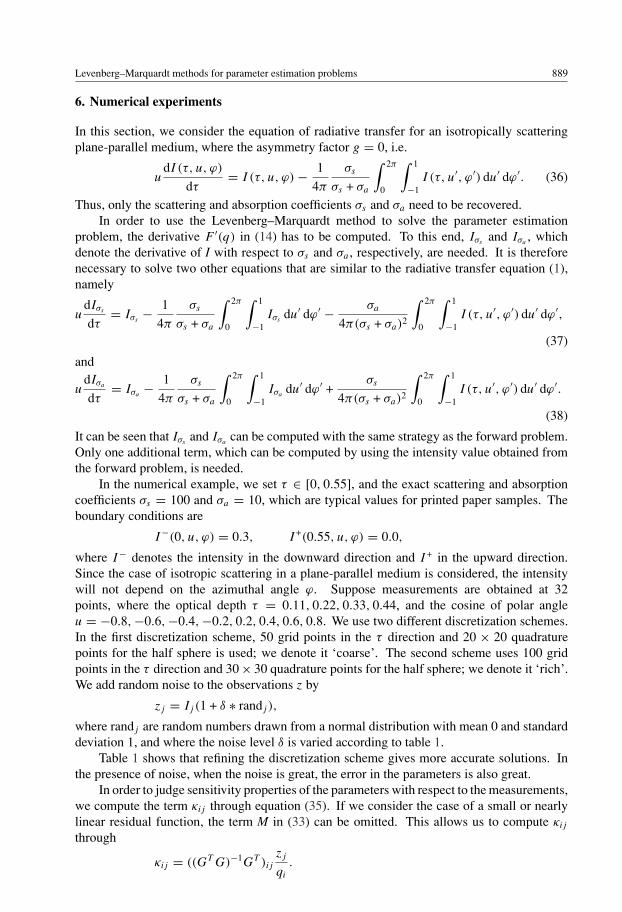
Levenberg–Marquardt methods for parameter estimation problems 889
6. Numerical experiments
In this section, we consider the equation of radiative transfer for an isotropically scatteringplane-parallel medium, where the asymmetry factor g = 0, i.e.
udI (τ, u, ϕ)
dτ= I (τ, u, ϕ) − 1
4π
σs
σs + σa
∫ 2π
0
∫ 1
−1I (τ, u′, ϕ′) du′ dϕ′. (36)
Thus, only the scattering and absorption coefficients σs and σa need to be recovered.In order to use the Levenberg–Marquardt method to solve the parameter estimation
problem, the derivative F ′(q) in (14) has to be computed. To this end, Iσsand Iσa
, whichdenote the derivative of I with respect to σs and σa , respectively, are needed. It is thereforenecessary to solve two other equations that are similar to the radiative transfer equation (1),namely
udIσs
dτ= Iσs
− 1
4π
σs
σs + σa
∫ 2π
0
∫ 1
−1Iσs
du′ dϕ′ − σa
4π(σs + σa)2
∫ 2π
0
∫ 1
−1I (τ, u′, ϕ′) du′ dϕ′,
(37)
and
udIσa
dτ= Iσa
− 1
4π
σs
σs + σa
∫ 2π
0
∫ 1
−1Iσa
du′ dϕ′ +σs
4π(σs + σa)2
∫ 2π
0
∫ 1
−1I (τ, u′, ϕ′) du′ dϕ′.
(38)
It can be seen that Iσsand Iσa
can be computed with the same strategy as the forward problem.Only one additional term, which can be computed by using the intensity value obtained fromthe forward problem, is needed.
In the numerical example, we set τ ∈ [0, 0.55], and the exact scattering and absorptioncoefficients σs = 100 and σa = 10, which are typical values for printed paper samples. Theboundary conditions are
I−(0, u, ϕ) = 0.3, I+(0.55, u, ϕ) = 0.0,
where I− denotes the intensity in the downward direction and I + in the upward direction.Since the case of isotropic scattering in a plane-parallel medium is considered, the intensitywill not depend on the azimuthal angle ϕ. Suppose measurements are obtained at 32points, where the optical depth τ = 0.11, 0.22, 0.33, 0.44, and the cosine of polar angleu = −0.8,−0.6,−0.4,−0.2, 0.2, 0.4, 0.6, 0.8. We use two different discretization schemes.In the first discretization scheme, 50 grid points in the τ direction and 20 × 20 quadraturepoints for the half sphere is used; we denote it ‘coarse’. The second scheme uses 100 gridpoints in the τ direction and 30 × 30 quadrature points for the half sphere; we denote it ‘rich’.We add random noise to the observations z by
zj = Ij (1 + δ ∗ randj ),
where randj are random numbers drawn from a normal distribution with mean 0 and standarddeviation 1, and where the noise level δ is varied according to table 1.
Table 1 shows that refining the discretization scheme gives more accurate solutions. Inthe presence of noise, when the noise is great, the error in the parameters is also great.
In order to judge sensitivity properties of the parameters with respect to the measurements,we compute the term κij through equation (35). If we consider the case of a small or nearlylinear residual function, the term M in (33) can be omitted. This allows us to compute κij
through
κij = ((GT G)−1GT )ijzj
qi
.
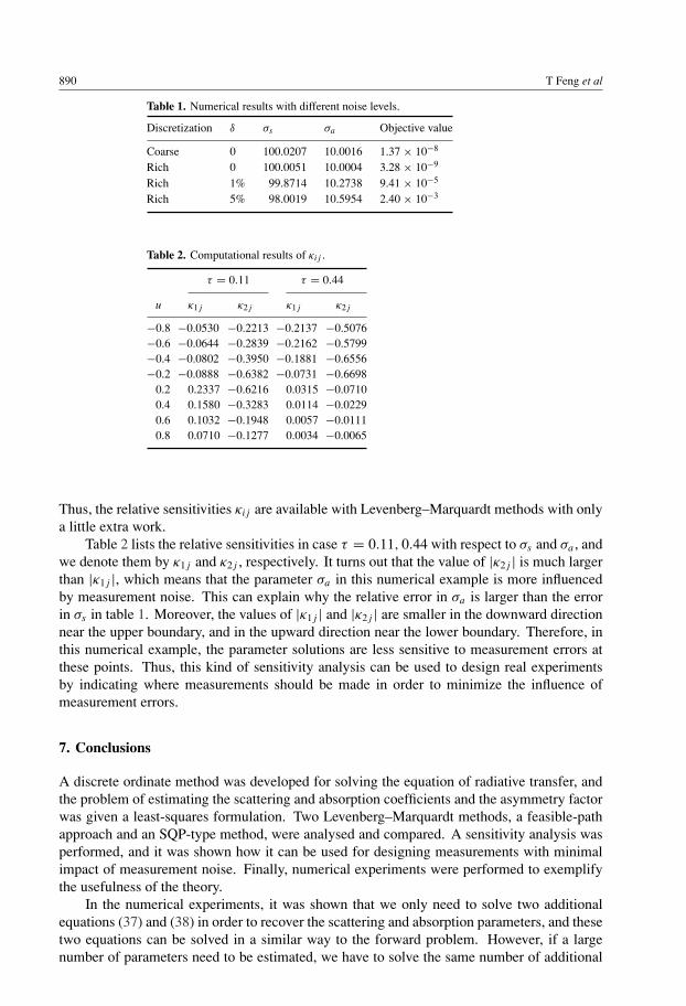
890 T Feng et al
Table 1. Numerical results with different noise levels.
Discretization δ σs σa Objective value
Coarse 0 100.0207 10.0016 1.37 × 10⁻⁸
Rich 0 100.0051 10.0004 3.28 × 10⁻⁹
Rich 1% 99.8714 10.2738 9.41 × 10⁻⁵
Rich 5% 98.0019 10.5954 2.40 × 10⁻³
Table 2. Computational results of κij .
τ = 0.11 τ = 0.44
u κ1j κ2j κ1j κ2j
−0.8 −0.0530 −0.2213 −0.2137 −0.5076−0.6 −0.0644 −0.2839 −0.2162 −0.5799−0.4 −0.0802 −0.3950 −0.1881 −0.6556−0.2 −0.0888 −0.6382 −0.0731 −0.6698
0.2 0.2337 −0.6216 0.0315 −0.07100.4 0.1580 −0.3283 0.0114 −0.02290.6 0.1032 −0.1948 0.0057 −0.01110.8 0.0710 −0.1277 0.0034 −0.0065
Thus, the relative sensitivities κij are available with Levenberg–Marquardt methods with onlya little extra work.
Table 2 lists the relative sensitivities in case τ = 0.11, 0.44 with respect to σs and σa , andwe denote them by κ1j and κ2j , respectively. It turns out that the value of |κ2j | is much largerthan |κ1j |, which means that the parameter σa in this numerical example is more influencedby measurement noise. This can explain why the relative error in σa is larger than the errorin σs in table 1. Moreover, the values of |κ1j | and |κ2j | are smaller in the downward directionnear the upper boundary, and in the upward direction near the lower boundary. Therefore, inthis numerical example, the parameter solutions are less sensitive to measurement errors atthese points. Thus, this kind of sensitivity analysis can be used to design real experimentsby indicating where measurements should be made in order to minimize the influence ofmeasurement errors.
7. Conclusions
A discrete ordinate method was developed for solving the equation of radiative transfer, andthe problem of estimating the scattering and absorption coefficients and the asymmetry factorwas given a least-squares formulation. Two Levenberg–Marquardt methods, a feasible-pathapproach and an SQP-type method, were analysed and compared. A sensitivity analysis wasperformed, and it was shown how it can be used for designing measurements with minimalimpact of measurement noise. Finally, numerical experiments were performed to exemplifythe usefulness of the theory.
In the numerical experiments, it was shown that we only need to solve two additionalequations (37) and (38) in order to recover the scattering and absorption parameters, and thesetwo equations can be solved in a similar way to the forward problem. However, if a largenumber of parameters need to be estimated, we have to solve the same number of additional
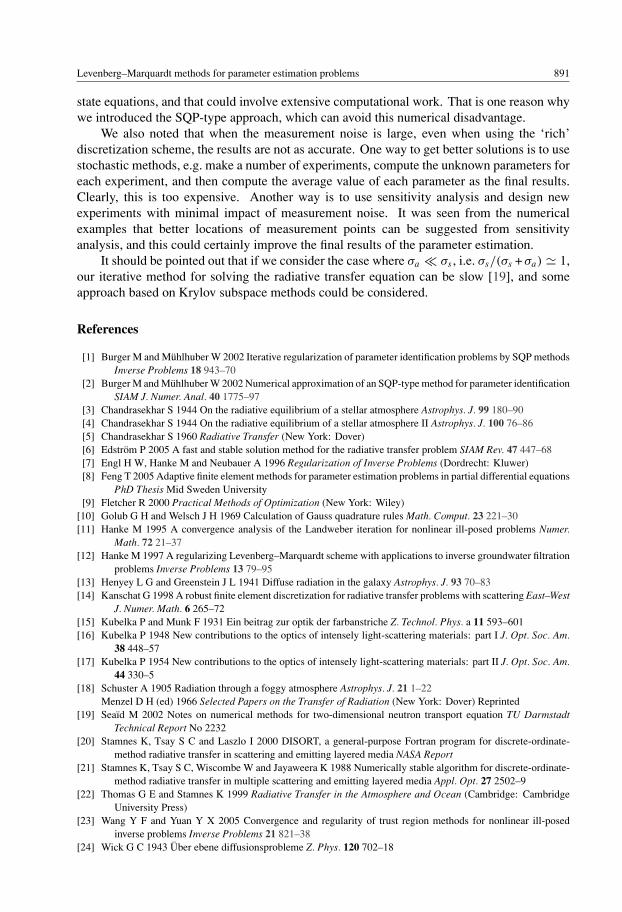
Levenberg–Marquardt methods for parameter estimation problems 891
state equations, and that could involve extensive computational work. That is one reason whywe introduced the SQP-type approach, which can avoid this numerical disadvantage.
We also noted that when the measurement noise is large, even when using the ‘rich’discretization scheme, the results are not as accurate. One way to get better solutions is to usestochastic methods, e.g. make a number of experiments, compute the unknown parameters foreach experiment, and then compute the average value of each parameter as the final results.Clearly, this is too expensive. Another way is to use sensitivity analysis and design newexperiments with minimal impact of measurement noise. It was seen from the numericalexamples that better locations of measurement points can be suggested from sensitivityanalysis, and this could certainly improve the final results of the parameter estimation.
It should be pointed out that if we consider the case where σa σs , i.e. σs/(σs + σa) � 1,our iterative method for solving the radiative transfer equation can be slow [19], and someapproach based on Krylov subspace methods could be considered.
References
[1] Burger M and Muhlhuber W 2002 Iterative regularization of parameter identification problems by SQP methodsInverse Problems 18 943–70
[2] Burger M and Muhlhuber W 2002 Numerical approximation of an SQP-type method for parameter identificationSIAM J. Numer. Anal. 40 1775–97
[3] Chandrasekhar S 1944 On the radiative equilibrium of a stellar atmosphere Astrophys. J. 99 180–90[4] Chandrasekhar S 1944 On the radiative equilibrium of a stellar atmosphere II Astrophys. J. 100 76–86[5] Chandrasekhar S 1960 Radiative Transfer (New York: Dover)[6] Edstrom P 2005 A fast and stable solution method for the radiative transfer problem SIAM Rev. 47 447–68[7] Engl H W, Hanke M and Neubauer A 1996 Regularization of Inverse Problems (Dordrecht: Kluwer)[8] Feng T 2005 Adaptive finite element methods for parameter estimation problems in partial differential equations
PhD Thesis Mid Sweden University[9] Fletcher R 2000 Practical Methods of Optimization (New York: Wiley)
[10] Golub G H and Welsch J H 1969 Calculation of Gauss quadrature rules Math. Comput. 23 221–30[11] Hanke M 1995 A convergence analysis of the Landweber iteration for nonlinear ill-posed problems Numer.
Math. 72 21–37[12] Hanke M 1997 A regularizing Levenberg–Marquardt scheme with applications to inverse groundwater filtration
problems Inverse Problems 13 79–95[13] Henyey L G and Greenstein J L 1941 Diffuse radiation in the galaxy Astrophys. J. 93 70–83[14] Kanschat G 1998 A robust finite element discretization for radiative transfer problems with scattering East–West
J. Numer. Math. 6 265–72[15] Kubelka P and Munk F 1931 Ein beitrag zur optik der farbanstriche Z. Technol. Phys. a 11 593–601[16] Kubelka P 1948 New contributions to the optics of intensely light-scattering materials: part I J. Opt. Soc. Am.
38 448–57[17] Kubelka P 1954 New contributions to the optics of intensely light-scattering materials: part II J. Opt. Soc. Am.
44 330–5[18] Schuster A 1905 Radiation through a foggy atmosphere Astrophys. J. 21 1–22
Menzel D H (ed) 1966 Selected Papers on the Transfer of Radiation (New York: Dover) Reprinted[19] Seaıd M 2002 Notes on numerical methods for two-dimensional neutron transport equation TU Darmstadt
Technical Report No 2232[20] Stamnes K, Tsay S C and Laszlo I 2000 DISORT, a general-purpose Fortran program for discrete-ordinate-
method radiative transfer in scattering and emitting layered media NASA Report[21] Stamnes K, Tsay S C, Wiscombe W and Jayaweera K 1988 Numerically stable algorithm for discrete-ordinate-
method radiative transfer in multiple scattering and emitting layered media Appl. Opt. 27 2502–9[22] Thomas G E and Stamnes K 1999 Radiative Transfer in the Atmosphere and Ocean (Cambridge: Cambridge
University Press)[23] Wang Y F and Yuan Y X 2005 Convergence and regularity of trust region methods for nonlinear ill-posed
inverse problems Inverse Problems 21 821–38[24] Wick G C 1943 Uber ebene diffusionsprobleme Z. Phys. 120 702–18


VI

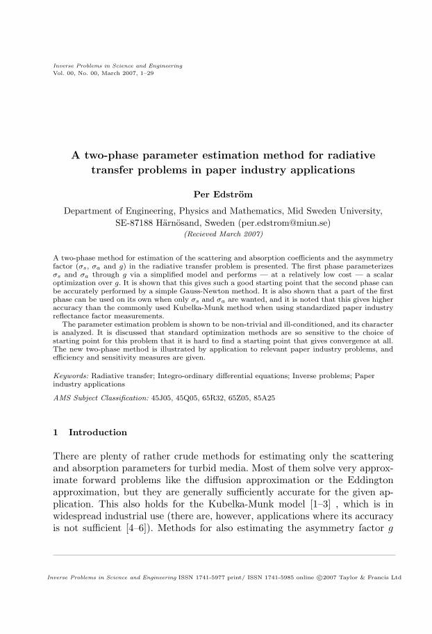
Inverse Problems in Science and EngineeringVol. 00, No. 00, March 2007, 1–29
A two-phase parameter estimation method for radiative
transfer problems in paper industry applications
Per Edstrom
Department of Engineering, Physics and Mathematics, Mid Sweden University,SE-87188 Harnosand, Sweden ([email protected])
(Recieved March 2007)
A two-phase method for estimation of the scattering and absorption coefficients and the asymmetryfactor (σs, σa and g) in the radiative transfer problem is presented. The first phase parameterizesσs and σa through g via a simplified model and performs — at a relatively low cost — a scalaroptimization over g. It is shown that this gives such a good starting point that the second phase canbe accurately performed by a simple Gauss-Newton method. It is also shown that a part of the firstphase can be used on its own when only σs and σa are wanted, and it is noted that this gives higheraccuracy than the commonly used Kubelka-Munk method when using standardized paper industryreflectance factor measurements.
The parameter estimation problem is shown to be non-trivial and ill-conditioned, and its characteris analyzed. It is discussed that standard optimization methods are so sensitive to the choice ofstarting point for this problem that it is hard to find a starting point that gives convergence at all.The new two-phase method is illustrated by application to relevant paper industry problems, andefficiency and sensitivity measures are given.
Keywords: Radiative transfer; Integro-ordinary differential equations; Inverse problems; Paperindustry applications
AMS Subject Classification: 45J05, 45Q05, 65R32, 65Z05, 85A25
1 Introduction
There are plenty of rather crude methods for estimating only the scatteringand absorption parameters for turbid media. Most of them solve very approx-imate forward problems like the diffusion approximation or the Eddingtonapproximation, but they are generally sufficiently accurate for the given ap-plication. This also holds for the Kubelka-Munk model [1–3] , which is inwidespread industrial use (there are, however, applications where its accuracyis not sufficient [4–6]). Methods for also estimating the asymmetry factor g
Inverse Problems in Science and Engineering ISSN 1741-5977 print/ ISSN 1741-5985 online c©2007 Taylor & Francis Ltd
2 P. Edstrom
are scarce, and even fewer are efficient and accurate. Most efforts come frommedical applications, while the industrial side has shown less interest so far.Van Gemert and Star [7] presented an attempt, but it included approximationsand boundary conditions that give it limited use. Prahl et. al [8] introducedthe inverse adding-doubling method, but reported on problems finding suit-able starting points. One recent interesting approach of high accuracy waspresented by Joshi et. al [9], but it suffers from very long computation times.In spite of the reported problems in the literature, this work aims to use onlysimple implementations of standard optimization methods for this parameterestimation problem, and still achieve good efficiency.
Estimating only the scattering and absorption parameters from reflectancemeasurements is straightforward in cruder two-flux problem formulations likeKubelka-Munk. However, more accurate estimation of more parameters is anoutstanding issue in more general radiative transfer problem formulations. Inthis work, the radiative transfer problem has an angle-resolved formulation,and a many-flux solution procedure is used. The parameter estimation problemis formulated as a least-squares optimization problem, and a two-phase methodfor its solution is implemented and evaluated. The successful recovery of σs,σa and g is illustrated by application to relevant paper industry problems.
The properties of the radiative transfer parameter estimation problem havenot yet been fully investigated. In order to interpret the results correctly, someknowledge of the influence of measurement errors or noise on the parametersis needed. This knowledge can also be used for the design of experiments withminimal influence from measurement errors. In this work, the curvature ofthe problem is investigated and a perturbation analysis is performed, and theresults of numerical experiments are discussed in the light of those findings.
This work will frequently distinguish between two problems that apply toboth the forward and the inverse settings. The full problem comprises angle-resolved data together with scattering, absorption and asymmetry parameters.The d/0 problem involves standardized reflectance factor data as used in thepaper industry [10–13], and scattering and absorption parameters only. Howto handle anisotropy is a new and open question for the paper industry, and re-fined measurement and simulation methods are needed to resolve this matter.This work is a step in that direction.
Section 2 gives a problem formulation and presents the solution methodsused in the forward problem. In Section 3, the inverse problem is formulated,the optimization methods used in the inverse calculations are discussed, andspecific solution methods to the d/0 and full inverse problems are suggested.The sensitivity analysis is performed in Section 4, numerical experiments arepresented in Section 5 on problem characteristics and in Section 6 on methodperformance. Section 7 gives a brief discussion of the findings.
Two-phase parameter estimation method 3
2 The forward problem
The radiative transfer problem considers the propagation of radiation in aturbid medium. The problem is often studied in a plane-parallel geometry,where the horizontal extension of the medium is assumed to be large enoughto give no boundary effects at the sides. At the top and bottom boundarysurfaces, boundary conditions are assumed to be time- and space-independent.The radiation is assumed to be monochromatic, and the scattering is assumedto be conservative, i.e. without change in frequency between incoming andoutgoing radiation. The medium is treated as a continuum of scattering andabsorption sites. Polarization effects are ignored, and what is left is then ascalar intensity, which is the variable to solve for.
2.1 Formulation
Edstrom [14] states the equation of radiative transfer as
udI(τ, u, ϕ)
dτ= I(τ, u, ϕ) − 1
4π
σs
σs + σa
∫ 2π
0
∫ 1
−1p(u′, ϕ′;u, ϕ)I(τ, u′, ϕ′)du′dϕ′.
(1)The unknown intensity I at optical depth τ is considered as non-interactingbeams of radiation in all directions. The scattering and absorption coefficientsof the medium are denoted by σs and σa, and the phase function p speci-fies the probability distribution of scattering from incident direction (u′, ϕ′)to direction (u, ϕ), where u is cosine of polar angle, and ϕ is azimuthal an-gle. The shape of the phase function is controlled by a parameter called theasymmetry factor, g, ranging from complete forward scattering (g = 1) overisotropic scattering (g = 0) to complete backward scattering (g = −1). Differ-ent phase functions have been proposed to describe physically different typesof scattering. This work considers the Henyey-Greenstein [15] phase function.It should not be seen as a real phase function, but is a one-parameter analyticalapproximation of widespread use. It is given by
p(cosΘ) =1 − g2
(1 + g2 − 2g cos Θ)3/2 , (2)
where Θ is the scattering angle. It is thus evident that the Henyey-Greensteinphase function is dependent on the scattering angle Θ only, and not on thespecific directions of incident and scattered radiation.
4 P. Edstrom
2.2 Solution methods
Dort2002 [14] is a radiative transfer solution method adapted to light scat-tering in paper and print. It is used to solve the full radiative transfer problemin this work. Dort2002 has been successively improved and evaluated [16],and has also been successfully applied to real paper industry problems [4–6].Dort2002 uses Fourier analysis on the azimuthal angle to turn the integro-differential equation (1) into a number of uncoupled equations, one for eachFourier component of the unknown intensity, which are then discretized usingnumerical quadrature. This yields a system of first order linear differentialequations for each Fourier component, and the natural solution proceduregives an eigenvalue problem.
In the Dort2002 solution method, the azimuthally averaged intensity isgiven by the 0th Fourier component. This quantity is all that is needed tocalculate the reflectance measures that result from using the d/0◦ instrumentgeometry that is standardized in the paper industry [10–13]. To solve thisd/0 problem, Dort2002 also contains a specialized solution method with thespecific purpose of performing such calculations at the highest possible speed.This gives a significant reduction in computation time compared to the fullmethod [16]. Since the standardized d/0◦ instrument geometry is specificallytaken into account in Dort2002, a higher accuracy is achieved than with theKubelka-Munk solution method that is normally used in the paper industry[4, 6]. Although only a side effect in the context of this work, this actuallymakes Dort2002 an alternative to Kubelka-Munk when higher accuracy isneeded.
It should be noted that the focus of this work is the inverse method. There-fore, other forward solution methods than Dort2002 could well be considered,and as long as they provide the same accuracy, the conclusions in this workstill hold. Replacing Dort2002 would probably increase computation timesthough, since it very efficiently provides intensities and reflectances for thepaper and printing applications studied here.
3 The parameter estimation problem
The full parameter estimation problem consists in determining σs, σa andg from angle-resolved intensity measurements in chosen directions, I(ui, ϕi).Such measurements are available from special goniophotometers. In the d/0problem, only σs and σa are estimated from standardized reflectance factormeasurements, R0 and R∞, using a chosen ad hoc value of g. Standardizedmeasurements with d/0◦ instrument geometry of reflectance factor are abun-dant in the paper industry. They use two measurements of the same sample,one over a black cavity and another over a thick pile of identical samples.
Two-phase parameter estimation method 5
The parameter estimation problem is to find parameter values that minimizesome distance measure between real measurements and model predictions. Thefull problem is usually over-determined with noisy measurements. The noisecan be controlled by averaging over several measurements, but the parameterestimation is nevertheless a nonzero-residual problem. The d/0 problem usestwo measurements to determine two parameters, which makes it a zero-residualproblem regardless of noise.
3.1 Formulation
One way to introduce the distance measure to minimize is through an objectivefunction that sums squared errors, such as
F (x) =12||f(x)||22 =
12
∑i
fi(x)2 =12
∑i
{Mi(x) − bi}2, (3)
where i denotes the respective quantity (be it intensity in a given direction orreflectance factor over a given background), and x is the vector of parametersto be determined. This formulation is statistically optimal if the measurementerrors are normally distributed, which may reasonably be considered to be thecase here. In this work, the model predictions Mi(x) are given by Dort2002
simulations, and bi are given by goniophotometer or d/0◦ instrument geometrymeasurements. An obvious formulation of the parameter estimation problemis then
minx
F (x), (4)
or the explicit least-squares formulation
minx
12||f(x)||22 = min
x
12
∑i
fi(x)2. (5)
If one defines the set of permissible parameter combinations as
S = {(σs, σa, g) : σs > 0, σa > 0,−1 < g < 1}, (6)
one can state the parameter estimation problem in various ways, which makesit possible to use different optimization methods to find a solution. Of course,since the problem is constrained by
x ∈ S, (7)
6 P. Edstrom
one needs to deal with this separately if unconstrained formulations are used.It should be pointed out that it is assumed throughout this work that the
model output — or the measurement — is given uniquely from the parameters.This is a quite reasonable assumption, especially for applied problems, butnevertheless it has never been proved in general; indeed, not much at all isknown regarding existence and uniqueness for the general radiative transferproblem.
3.2 Solution methods
A few simple implementations of standard optimization methods were imple-mented as described below, and comparison was also made to some MatlabOptimization Toolbox functions as examples of commercial solvers. In the fol-lowing, k designates the iteration index.
3.2.1 Newton. With an unconstrained minimization formulation like (4), aclassical approach is Newton’s method. The typical Newton iteration consistsof determining a search direction, pk, by solving
∇2xxF (xk)pk = −∇xF (xk), (8)
and then updating the solution estimate through
xk+1 = xk + αkpk. (9)
The step size parameter, αk, is normally chosen in a line search procedure.The constant step size αk = 1 gives the pure form of Newton’s method. Neara nonsingular minimum, the Hessian ∇2
xxF (xk) will be positive definite, andthe convergence will be quadratic. The good convergence comes at the costof expensive calculation of the Hessian. On the other hand, far from such alocal minimum, the Hessian may be singular or the search direction may notbe a decent direction because the Hessian is not positive definite. Thus, unlessa very good starting point is available, the convergence may initially be verypoor. The convergence also depends on the condition of the Hessian in thesolution.
In this work, a Newton method was implemented with a forward differencescheme for the gradient and the Hessian. The constraints (7) were kept bylimiting pk in the (rare) cases where xk+pk �∈ S. Then an Armijo condition [17]was used for choosing step size in the line search. The convergence criterion was||∇xF (xk)|| <
√εmach (1 + |F (xk)|), where εmach is the floating point relative
accuracy of the machine, as suggested for example by Nash and Sofer [18].
Two-phase parameter estimation method 7
The algorithm was as follows.
Algorithm 1 (Newton)Choose starting point x
repeat until convergence or failureConvergence and failure checkCalculate gradient G by forward differencesCalculate Hessian H by forward differencesCalculate search direction p by solving Hp = −G through factorizationSet step length α = 1, then half α until Armijo condition fulfilledUpdate x = x + αp
end
From a purely numerical point of view, different finite difference intervals,h, were used for the gradient (about the square root of machine precision) andHessian (a few decades larger) approximations for the most accurate results[19].
3.2.2 Quasi-Newton. Newton’s method computes the full Hessian in eachiteration, which is expensive. An alternative is to continuously update an ap-proximation of the Hessian, and thereby approximate the Newton direction.Quasi-Newton methods do this by building curvature information from thesuccessive iterates xk and the corresponding gradients ∇xF (xk) to formulatea quadratic model problem. The idea is to avoid the second derivative calcu-lations, while still maintaining good convergence since the Hessian is progres-sively approached. There are a large number of Hessian updating methods, butthe BFGS method [20–23] is considered to be the best for general purposes.Quasi-Newton methods have the advantage that they always give descent.A possible drawback however, is that inaccurate derivative information mayaccumulate errors.
In this work, a quasi-Newton method was implemented exactly as the New-ton method in Section 3.2.1, but with the Hessian approximated through aBFGS update. The starting estimate of the Hessian was, for positive defi-niteness, calculated through the Jacobian as described for Gauss-Newton inSection 3.2.3. The algorithm was as follows.
Algorithm 2 (Quasi-Newton)Choose starting point x
Calculate Gauss-Newton Jacobian J at start by forward differencesCalculate Hessian by H = JT J
8 P. Edstrom
repeat until convergence or failureConvergence and failure checkCalculate gradient G by forward differencesCalculate search direction p by solving Hp = −G through factorizationSet step length α = 1, then half α until Armijo condition fulfilledUpdate x = x + αp
Update Hessian H by BFGS methodend
3.2.3 Gauss-Newton. With a least-squares formulation like (5), a special-ized method is Gauss-Newton [24]. The Gauss-Newton iteration is based onthe idea of linearizing f around the point xk to obtain the linear least-squaresproblem
minpk
12||f(xk) + J(xk)pk||22, (10)
where J is the Jacobian of f . This is then solved for pk, for example by usinga QR factorization.
Formally, although not normally used in solution methods, the search direc-tion is found through the normal equations
J(xk)T J(xk)pk = −J(xk)T f(xk). (11)
Through this the Gauss-Newton method can be compared with Newton’smethod. The search direction equation (11) is actually the same as Eq. (8),where the gradient is given by
G(xk) = J(xk)T f(xk) (12)
and the Jacobian is used to approximate the Hessian through
H(xk) ≈ J(xk)T J(xk). (13)
Gauss-Newton saves computations — by not computing the Hessian — possi-bly at the expense of decreased convergence rate. Near a solution the conver-gence is quadratic for zero-residual problems if J has full rank in the solution.The difference between the Hessian and its Gauss-Newton approximation canbe shown to be
∑i fi(x)f ′′
i (x), see Eq. (27). Hence, if the residual fi(x) orcurvature f ′′
i (x) is large, or if the Jacobian is ill-conditioned in an iteration or
Two-phase parameter estimation method 9
in the solution, Gauss-Newton may converge slowly or not at all. In such casesthe Newton method will be better. On the other hand, if the measurementsare noisy, Gauss-Newton may have a regularizing effect by omitting the term∑
i fi(x)f ′′i (x).
It can be noted from Eq. (11) that if J is square and has full rank, as in thed/0 case, the problem of finding the search direction can be reduced. In thiscase, the linearization of the problem (5) does not even need to be formulatedas a least-squares problem (10), but can be reduced to solving — with zeroresidual — the linear system
J(xk)pk = −f(xk) (14)
through Gaussian elimination. However, the full problem is over-determined,so the least-squares formulation is needed there.
In this work, a Gauss-Newton method was implemented with a forwarddifference scheme for the Jacobian, and an Armijo condition was used forchoosing step size in the line search. The constraints (7) were kept by limitingpk in the (rare) cases where xk + pk �∈ S. The algorithm was as follows.
Algorithm 3 (Gauss-Newton)
Choose starting point x
repeat until convergence or failure
Convergence and failure check
Calculate Jacobian J by forward differences
Calculate p by solving min||f + Jp||22 through QR factorization
Set step length α = 1, then half α until Armijo condition fulfilled
Update x = x + αp
end
3.2.4 Matlab Optimization Toolbox functions. The functions lsqnonlinand fmincon provided in Matlab Optimization Toolbox were tested ascommercial examples of constrained optimization methods. The functionlsqnonlin solves nonlinear least-squares problems using the Gauss-Newtonmethod with a mixed quadratic and cubic line search procedure. The functionfmincon uses a sequential quadratic programming (SQP) method [25], whichis related to Newton’s method. At each iteration, a positive definite quasi-Newton approximation of the Hessian is calculated using the BFGS method.This is then used to generate a quadratic programming (QP) subproblemwhose solution is used to form a search direction for a line search procedure.
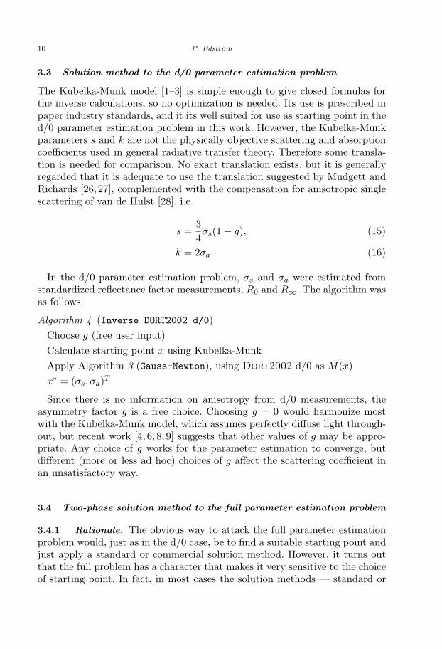
10 P. Edstrom
3.3 Solution method to the d/0 parameter estimation problem
The Kubelka-Munk model [1–3] is simple enough to give closed formulas forthe inverse calculations, so no optimization is needed. Its use is prescribed inpaper industry standards, and it its well suited for use as starting point in thed/0 parameter estimation problem in this work. However, the Kubelka-Munkparameters s and k are not the physically objective scattering and absorptioncoefficients used in general radiative transfer theory. Therefore some transla-tion is needed for comparison. No exact translation exists, but it is generallyregarded that it is adequate to use the translation suggested by Mudgett andRichards [26, 27], complemented with the compensation for anisotropic singlescattering of van de Hulst [28], i.e.
s =34σs(1 − g), (15)
k = 2σa. (16)
In the d/0 parameter estimation problem, σs and σa were estimated fromstandardized reflectance factor measurements, R0 and R∞. The algorithm wasas follows.
Algorithm 4 (Inverse DORT2002 d/0)Choose g (free user input)Calculate starting point x using Kubelka-MunkApply Algorithm 3 (Gauss-Newton), using Dort2002 d/0 as M(x)x∗ = (σs, σa)T
Since there is no information on anisotropy from d/0 measurements, theasymmetry factor g is a free choice. Choosing g = 0 would harmonize mostwith the Kubelka-Munk model, which assumes perfectly diffuse light through-out, but recent work [4, 6, 8, 9] suggests that other values of g may be appro-priate. Any choice of g works for the parameter estimation to converge, butdifferent (more or less ad hoc) choices of g affect the scattering coefficient inan unsatisfactory way.
3.4 Two-phase solution method to the full parameter estimation problem
3.4.1 Rationale. The obvious way to attack the full parameter estimationproblem would, just as in the d/0 case, be to find a suitable starting point andjust apply a standard or commercial solution method. However, it turns outthat the full problem has a character that makes it very sensitive to the choiceof starting point. In fact, in most cases the solution methods — standard or
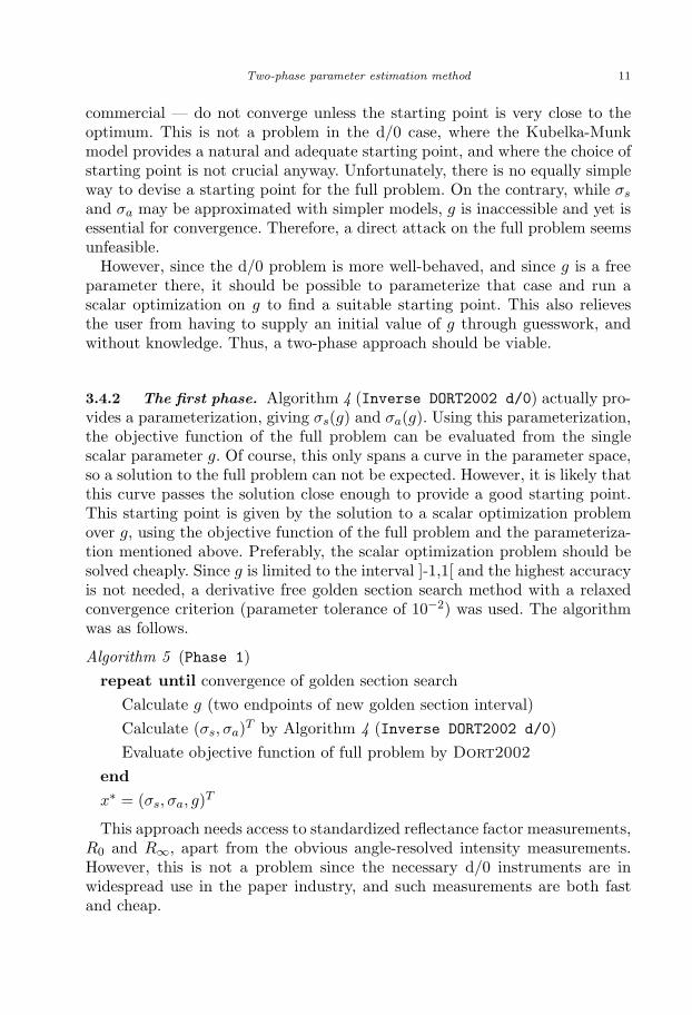
Two-phase parameter estimation method 11
commercial — do not converge unless the starting point is very close to theoptimum. This is not a problem in the d/0 case, where the Kubelka-Munkmodel provides a natural and adequate starting point, and where the choice ofstarting point is not crucial anyway. Unfortunately, there is no equally simpleway to devise a starting point for the full problem. On the contrary, while σs
and σa may be approximated with simpler models, g is inaccessible and yet isessential for convergence. Therefore, a direct attack on the full problem seemsunfeasible.
However, since the d/0 problem is more well-behaved, and since g is a freeparameter there, it should be possible to parameterize that case and run ascalar optimization on g to find a suitable starting point. This also relievesthe user from having to supply an initial value of g through guesswork, andwithout knowledge. Thus, a two-phase approach should be viable.
3.4.2 The first phase. Algorithm 4 (Inverse DORT2002 d/0) actually pro-vides a parameterization, giving σs(g) and σa(g). Using this parameterization,the objective function of the full problem can be evaluated from the singlescalar parameter g. Of course, this only spans a curve in the parameter space,so a solution to the full problem can not be expected. However, it is likely thatthis curve passes the solution close enough to provide a good starting point.This starting point is given by the solution to a scalar optimization problemover g, using the objective function of the full problem and the parameteriza-tion mentioned above. Preferably, the scalar optimization problem should besolved cheaply. Since g is limited to the interval ]-1,1[ and the highest accuracyis not needed, a derivative free golden section search method with a relaxedconvergence criterion (parameter tolerance of 10−2) was used. The algorithmwas as follows.
Algorithm 5 (Phase 1)repeat until convergence of golden section search
Calculate g (two endpoints of new golden section interval)Calculate (σs, σa)T by Algorithm 4 (Inverse DORT2002 d/0)Evaluate objective function of full problem by Dort2002
endx∗ = (σs, σa, g)T
This approach needs access to standardized reflectance factor measurements,R0 and R∞, apart from the obvious angle-resolved intensity measurements.However, this is not a problem since the necessary d/0 instruments are inwidespread use in the paper industry, and such measurements are both fastand cheap.
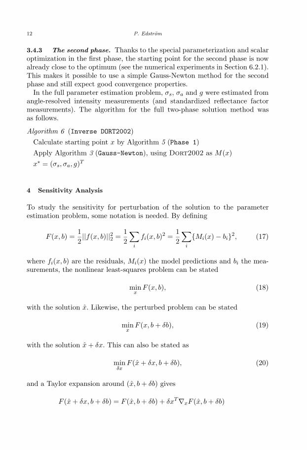
12 P. Edstrom
3.4.3 The second phase. Thanks to the special parameterization and scalaroptimization in the first phase, the starting point for the second phase is nowalready close to the optimum (see the numerical experiments in Section 6.2.1).This makes it possible to use a simple Gauss-Newton method for the secondphase and still expect good convergence properties.
In the full parameter estimation problem, σs, σa and g were estimated fromangle-resolved intensity measurements (and standardized reflectance factormeasurements). The algorithm for the full two-phase solution method wasas follows.
Algorithm 6 (Inverse DORT2002)Calculate starting point x by Algorithm 5 (Phase 1)Apply Algorithm 3 (Gauss-Newton), using Dort2002 as M(x)x∗ = (σs, σa, g)T
4 Sensitivity Analysis
To study the sensitivity for perturbation of the solution to the parameterestimation problem, some notation is needed. By defining
F (x, b) =12||f(x, b)||22 =
12
∑i
fi(x, b)2 =12
∑i
{Mi(x) − bi}2, (17)
where fi(x, b) are the residuals, Mi(x) the model predictions and bi the mea-surements, the nonlinear least-squares problem can be stated
minx
F (x, b), (18)
with the solution x. Likewise, the perturbed problem can be stated
minx
F (x, b + δb), (19)
with the solution x + δx. This can also be stated as
minδx
F (x + δx, b + δb), (20)
and a Taylor expansion around (x, b + δb) gives
F (x + δx, b + δb) = F (x, b + δb) + δxT∇xF (x, b + δb)
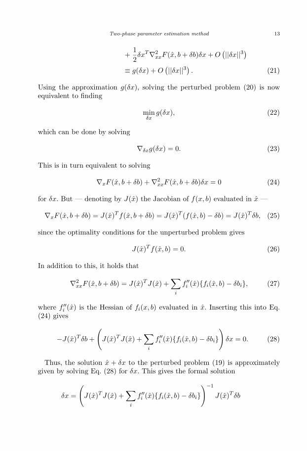
Two-phase parameter estimation method 13
+12δxT∇2
xxF (x, b + δb)δx + O(||δx||3)
≡ g(δx) + O(||δx||3) . (21)
Using the approximation g(δx), solving the perturbed problem (20) is nowequivalent to finding
minδx
g(δx), (22)
which can be done by solving
∇δxg(δx) = 0. (23)
This is in turn equivalent to solving
∇xF (x, b + δb) + ∇2xxF (x, b + δb)δx = 0 (24)
for δx. But — denoting by J(x) the Jacobian of f(x, b) evaluated in x —
∇xF (x, b + δb) = J(x)T f(x, b + δb) = J(x)T (f(x, b) − δb) = J(x)T δb, (25)
since the optimality conditions for the unperturbed problem gives
J(x)T f(x, b) = 0. (26)
In addition to this, it holds that
∇2xxF (x, b + δb) = J(x)T J(x) +
∑i
f ′′i (x){fi(x, b) − δbi}, (27)
where f ′′i (x) is the Hessian of fi(x, b) evaluated in x. Inserting this into Eq.
(24) gives
−J(x)T δb +
(J(x)T J(x) +
∑i
f ′′i (x){fi(x, b) − δbi}
)δx = 0. (28)
Thus, the solution x + δx to the perturbed problem (19) is approximatelygiven by solving Eq. (28) for δx. This gives the formal solution
δx =
(J(x)T J(x) +
∑i
f ′′i (x){fi(x, b) − δbi}
)−1
J(x)T δb
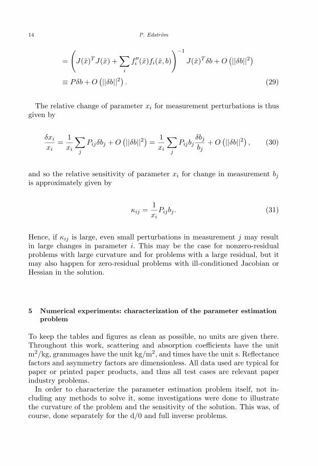
14 P. Edstrom
=
(J(x)T J(x) +
∑i
f ′′i (x)fi(x, b)
)−1
J(x)T δb + O(||δb||2)
≡ Pδb + O(||δb||2) . (29)
The relative change of parameter xi for measurement perturbations is thusgiven by
δxi
xi=
1xi
∑j
Pijδbj + O(||δb||2) =
1xi
∑j
Pijbjδbj
bj+ O
(||δb||2) , (30)
and so the relative sensitivity of parameter xi for change in measurement bj
is approximately given by
κij =1xi
Pijbj . (31)
Hence, if κij is large, even small perturbations in measurement j may resultin large changes in parameter i. This may be the case for nonzero-residualproblems with large curvature and for problems with a large residual, but itmay also happen for zero-residual problems with ill-conditioned Jacobian orHessian in the solution.
5 Numerical experiments: characterization of the parameter estimationproblem
To keep the tables and figures as clean as possible, no units are given there.Throughout this work, scattering and absorption coefficients have the unitm2/kg, grammages have the unit kg/m2, and times have the unit s. Reflectancefactors and asymmetry factors are dimensionless. All data used are typical forpaper or printed paper products, and thus all test cases are relevant paperindustry problems.
In order to characterize the parameter estimation problem itself, not in-cluding any methods to solve it, some investigations were done to illustratethe curvature of the problem and the sensitivity of the solution. This was, ofcourse, done separately for the d/0 and full inverse problems.
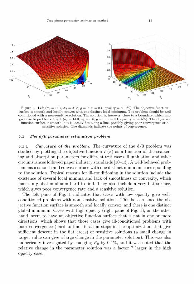
Two-phase parameter estimation method 15
020
4060
801000
50
1000
0.2
0.4
0.6
0.8
1
σs
σa
020
4060
80100
020
4060
80100
0
0.2
0.4
0.6
0.8
1
σsσ
a
Figure 1. Left (σs = 14.7, σa = 0.03, g = 0, w = 0.1, opacity = 50.1%): The objective functionsurface is smooth and locally convex with one distinct local minimum. The problem should be wellconditioned with a non-sensitive solution. The solution is, however, close to a boundary, which maygive rise to problems. Right (σs = 14.0, σa = 5.6, g = 0, w = 0.1, opacity = 95.5%): The objectivefunction surface is smooth, but is locally flat along a line, possibly giving poor convergence or a
sensitive solution. The diamonds indicate the points of convergence.
5.1 The d/0 parameter estimation problem
5.1.1 Curvature of the problem. The curvature of the d/0 problem wasstudied by plotting the objective function F (x) as a function of the scatter-ing and absorption parameters for different test cases. Illumination and othercircumstances followed paper industry standards [10–13]. A well-behaved prob-lem has a smooth and convex surface with one distinct minimum correspondingto the solution. Typical reasons for ill-conditioning in the solution include theexistence of several local minima and lack of smoothness or convexity, whichmakes a global minimum hard to find. They also include a very flat surface,which gives poor convergence rate and a sensitive solution.
The left pane of Fig. 1 indicates that cases with low opacity give well-conditioned problems with non-sensitive solutions. This is seen since the ob-jective function surface is smooth and locally convex, and there is one distinctglobal minimum. Cases with high opacity (right pane of Fig. 1), on the otherhand, seem to have an objective function surface that is flat in one or moredirections, which shows that those cases give ill-conditioned problems withpoor convergence (hard to find iteration steps in the optimization that givesufficient descent in the flat areas) or sensitive solutions (a small change intarget value can give a large change in the parameter solution). This was alsonumerically investigated by changing R0 by 0.1%, and it was noted that therelative change in the parameter solution was a factor 7 larger in the highopacity case.
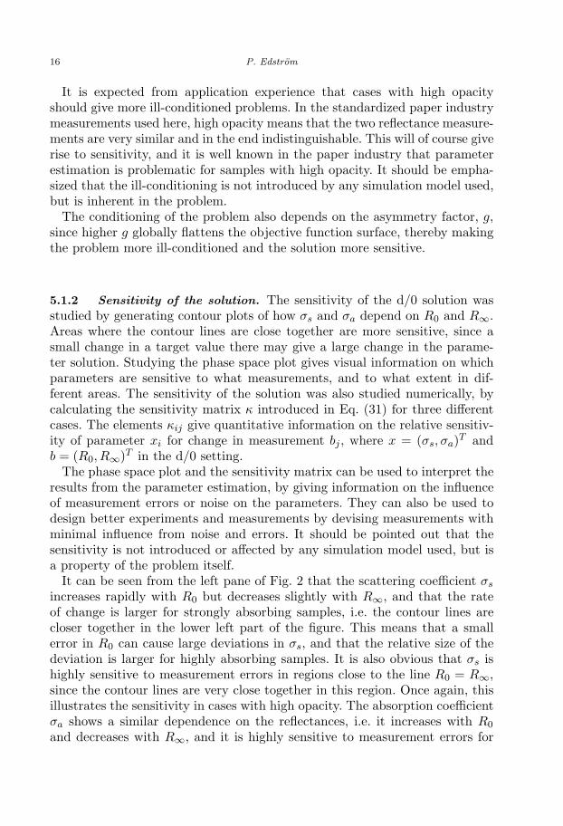
16 P. Edstrom
It is expected from application experience that cases with high opacityshould give more ill-conditioned problems. In the standardized paper industrymeasurements used here, high opacity means that the two reflectance measure-ments are very similar and in the end indistinguishable. This will of course giverise to sensitivity, and it is well known in the paper industry that parameterestimation is problematic for samples with high opacity. It should be empha-sized that the ill-conditioning is not introduced by any simulation model used,but is inherent in the problem.
The conditioning of the problem also depends on the asymmetry factor, g,since higher g globally flattens the objective function surface, thereby makingthe problem more ill-conditioned and the solution more sensitive.
5.1.2 Sensitivity of the solution. The sensitivity of the d/0 solution wasstudied by generating contour plots of how σs and σa depend on R0 and R∞.Areas where the contour lines are close together are more sensitive, since asmall change in a target value there may give a large change in the parame-ter solution. Studying the phase space plot gives visual information on whichparameters are sensitive to what measurements, and to what extent in dif-ferent areas. The sensitivity of the solution was also studied numerically, bycalculating the sensitivity matrix κ introduced in Eq. (31) for three differentcases. The elements κij give quantitative information on the relative sensitiv-ity of parameter xi for change in measurement bj , where x = (σs, σa)T andb = (R0, R∞)T in the d/0 setting.
The phase space plot and the sensitivity matrix can be used to interpret theresults from the parameter estimation, by giving information on the influenceof measurement errors or noise on the parameters. They can also be used todesign better experiments and measurements by devising measurements withminimal influence from noise and errors. It should be pointed out that thesensitivity is not introduced or affected by any simulation model used, but isa property of the problem itself.
It can be seen from the left pane of Fig. 2 that the scattering coefficient σs
increases rapidly with R0 but decreases slightly with R∞, and that the rateof change is larger for strongly absorbing samples, i.e. the contour lines arecloser together in the lower left part of the figure. This means that a smallerror in R0 can cause large deviations in σs, and that the relative size of thedeviation is larger for highly absorbing samples. It is also obvious that σs ishighly sensitive to measurement errors in regions close to the line R0 = R∞,since the contour lines are very close together in this region. Once again, thisillustrates the sensitivity in cases with high opacity. The absorption coefficientσa shows a similar dependence on the reflectances, i.e. it increases with R0and decreases with R∞, and it is highly sensitive to measurement errors for
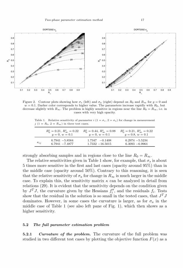
Figure 2. Contour plots showing how σs (left) and σa (right) depend on R0 and R∞ for g = 0 andw = 0.1. Darker color corresponds to higher value. The parameters increase rapidly with R0, but
decrease slightly with R∞. The problem is highly sensitive in regions near the line R0 = R∞, i.e. incases with very high opacity.
Table 1. Relative sensitivity of parameter i (1 = σs, 2 = σa) for change in measurementj (1 = R0, 2 = R∞) in three test cases.
R∗0 = 0.21, R∗∞ = 0.22 R∗
0 = 0.44, R∗∞ = 0.88 R∗0 = 0.21, R∗∞ = 0.22
g = 0, w = 0.1 g = 0, w = 0.1 g = 0.8, w = 0.1
κij6.7941 −5.85646.7941 −7.4877
1.7347 −0.14081.7332 −16.5015
6.2974 −5.52346.3093 −6.9964
strongly absorbing samples and in regions close to the line R0 = R∞.The relative sensitivities given in Table 1 show, for example, that σs is about
5 times more sensitive in the first and last cases (opacity around 95%) than inthe middle case (opacity around 50%). Contrary to this reasoning, it is seenthat the relative sensitivity of σa for change in R∞ is much larger in the middlecase. To explain this, the sensitivity matrix κ can be analyzed in detail fromrelations (29). It is evident that the sensitivity depends on the condition givenby JT J , the curvature given by the Hessians f ′′
i , and the residuals fi. Testsshow that the residual in the solution is so small in the tested cases, that JT Jdominates. However, in some cases the curvature is larger, as for σa in themiddle case of Table 1 (see also left pane of Fig. 1), which then shows as ahigher sensitivity.
5.2 The full parameter estimation problem
5.2.1 Curvature of the problem. The curvature of the full problem wasstudied in two different test cases by plotting the objective function F (x) as a
Two-phase parameter estimation method 17
1010
10
10
10
10
10
20
20
20
20
20
20
30
30
30
30
30
40
40
40
40
40
50
50
50
50
60
60
60
60
70
7070
70
80
80
8090
90
90
100
100
100
150150
200200
300400500
R∞
R0
DORT2002 σs
0.1 0.2 0.3 0.4 0.5 0.6 0.7 0.8 0.9
0.1
0.2
0.3
0.4
0.5
0.6
0.7
0.8
0.9
1
1
1
1
1
1
12
2
22
2
23
3
3
3
3
4
4
4
45
55
5
10
5
2
4
3
1
5
4
2
3
5
4
5
3
R∞
R0
DORT2002 σa
0.1 0.2 0.3 0.4 0.5 0.6 0.7 0.8 0.9
0.1
0.2
0.3
0.4
0.5
0.6
0.7
0.8
0.9
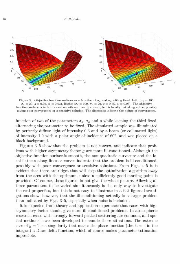
18 P. Edstrom
050
100150
200
0
10
20
30
40
50
0
0.2
0.4
0.6
0.8
1
σs
σa
050
100150
200
0
10
20
30
40
50
0
0.2
0.4
0.6
0.8
1
σs
σa
Figure 3. Objective function surfaces as a function of σs and σa with g fixed. Left: (σs = 100,σa = 20, g = 0.05, w = 0.03). Right: (σs = 100, σa = 20, g = 0.75, w = 0.03). The objective
function surface is in both cases smooth and nearly convex, but is locally flat along a line, possiblygiving poor convergence or a sensitive solution. The diamonds indicate the points of convergence.
function of two of the parameters σs, σa and g while keeping the third fixed,alternating the parameter to be fixed. The simulated sample was illuminatedby perfectly diffuse light of intensity 0.3 and by a beam (or collimated light)of intensity 1.0 with a polar angle of incidence of 60◦, and was placed on ablack background.
Figures 3–5 show that the problem is not convex, and indicate that prob-lems with higher asymmetry factor g are more ill-conditioned. Although theobjective function surface is smooth, the non-quadratic curvature and the lo-cal flatness along lines or curves indicate that the problem is ill-conditioned,possibly with poor convergence or sensitive solutions. From Figs. 4–5 it isevident that there are ridges that will keep the optimization algorithm awayfrom the area with the optimum, unless a sufficiently good starting point isprovided. Of course, these figures do not give the whole picture. Allowing allthree parameters to be varied simultaneously is the only way to investigatethe real properties, but this is not easy to illustrate in a flat figure. Investi-gations show, however, that the ill-conditioning actually is a larger problemthan indicated by Figs. 3–5, especially when noise is included.
It is expected from theory and application experience that cases with highasymmetry factor should give more ill-conditioned problems. In atmosphericresearch, cases with strongly forward peaked scattering are common, and spe-cial methods have been developed to handle those situations. The extremecase of g = 1 is a singularity that makes the phase function (the kernel in theintegral) a Dirac delta function, which of course makes parameter estimationimpossible.
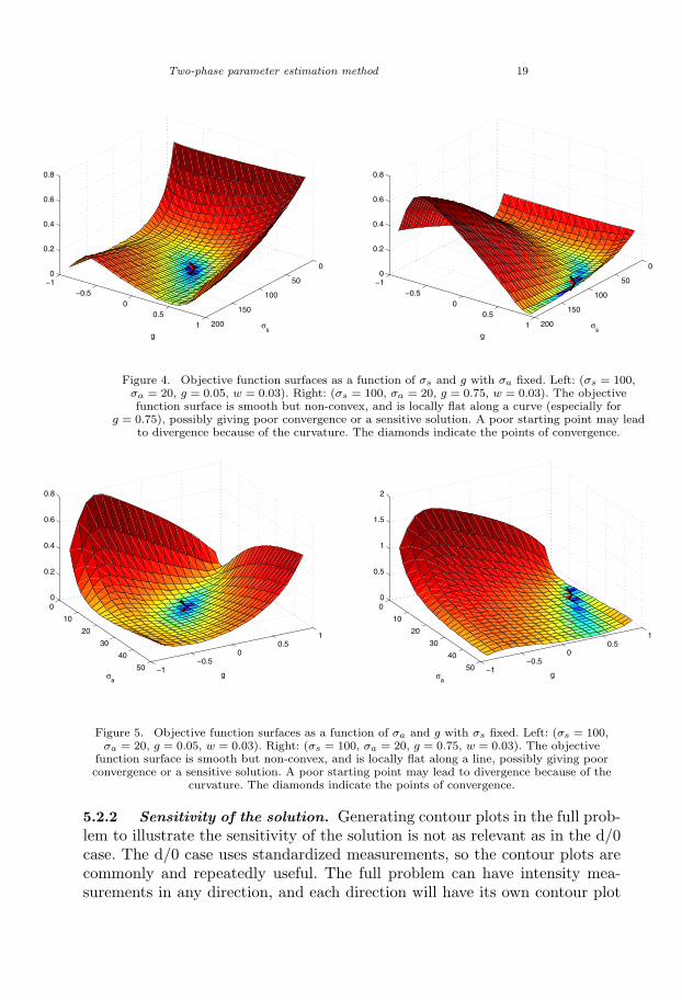
Two-phase parameter estimation method 19
0
50
100
150
200
−1−0.5
00.5
1
0
0.2
0.4
0.6
0.8
σs
g
0
50
100
150
200
−1−0.5
00.5
1
0
0.2
0.4
0.6
0.8
σs
g
Figure 4. Objective function surfaces as a function of σs and g with σa fixed. Left: (σs = 100,σa = 20, g = 0.05, w = 0.03). Right: (σs = 100, σa = 20, g = 0.75, w = 0.03). The objectivefunction surface is smooth but non-convex, and is locally flat along a curve (especially for
g = 0.75), possibly giving poor convergence or a sensitive solution. A poor starting point may leadto divergence because of the curvature. The diamonds indicate the points of convergence.
0
10
20
30
40
50 −1−0.5
00.5
1
0
0.2
0.4
0.6
0.8
gσa
0
10
20
30
40
50 −1−0.5
00.5
1
0
0.5
1
1.5
2
gσa
Figure 5. Objective function surfaces as a function of σa and g with σs fixed. Left: (σs = 100,σa = 20, g = 0.05, w = 0.03). Right: (σs = 100, σa = 20, g = 0.75, w = 0.03). The objective
function surface is smooth but non-convex, and is locally flat along a line, possibly giving poorconvergence or a sensitive solution. A poor starting point may lead to divergence because of the
curvature. The diamonds indicate the points of convergence.
5.2.2 Sensitivity of the solution. Generating contour plots in the full prob-lem to illustrate the sensitivity of the solution is not as relevant as in the d/0case. The d/0 case uses standardized measurements, so the contour plots arecommonly and repeatedly useful. The full problem can have intensity mea-surements in any direction, and each direction will have its own contour plot
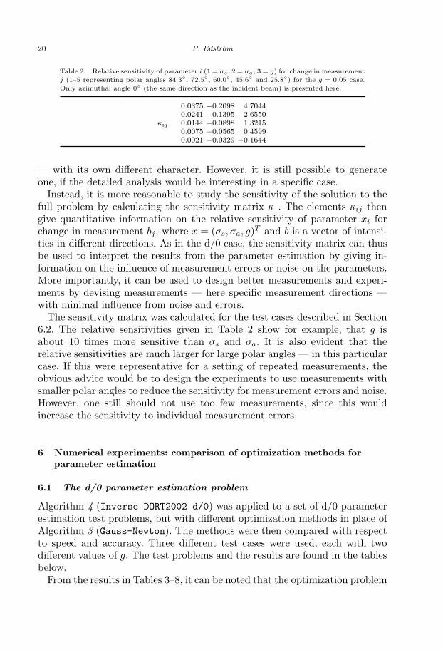
20 P. Edstrom
Table 2. Relative sensitivity of parameter i (1 = σs, 2 = σa, 3 = g) for change in measurementj (1–5 representing polar angles 84.3◦, 72.5◦, 60.0◦, 45.6◦ and 25.8◦) for the g = 0.05 case.Only azimuthal angle 0◦ (the same direction as the incident beam) is presented here.
κij
0.0375 −0.2098 4.70440.0241 −0.1395 2.65500.0144 −0.0898 1.32150.0075 −0.0565 0.45990.0021 −0.0329 −0.1644
— with its own different character. However, it is still possible to generateone, if the detailed analysis would be interesting in a specific case.
Instead, it is more reasonable to study the sensitivity of the solution to thefull problem by calculating the sensitivity matrix κ . The elements κij thengive quantitative information on the relative sensitivity of parameter xi forchange in measurement bj , where x = (σs, σa, g)T and b is a vector of intensi-ties in different directions. As in the d/0 case, the sensitivity matrix can thusbe used to interpret the results from the parameter estimation by giving in-formation on the influence of measurement errors or noise on the parameters.More importantly, it can be used to design better measurements and experi-ments by devising measurements — here specific measurement directions —with minimal influence from noise and errors.
The sensitivity matrix was calculated for the test cases described in Section6.2. The relative sensitivities given in Table 2 show for example, that g isabout 10 times more sensitive than σs and σa. It is also evident that therelative sensitivities are much larger for large polar angles — in this particularcase. If this were representative for a setting of repeated measurements, theobvious advice would be to design the experiments to use measurements withsmaller polar angles to reduce the sensitivity for measurement errors and noise.However, one still should not use too few measurements, since this wouldincrease the sensitivity to individual measurement errors.
6 Numerical experiments: comparison of optimization methods forparameter estimation
6.1 The d/0 parameter estimation problem
Algorithm 4 (Inverse DORT2002 d/0) was applied to a set of d/0 parameterestimation test problems, but with different optimization methods in place ofAlgorithm 3 (Gauss-Newton). The methods were then compared with respectto speed and accuracy. Three different test cases were used, each with twodifferent values of g. The test problems and the results are found in the tablesbelow.
From the results in Tables 3–8, it can be noted that the optimization problem
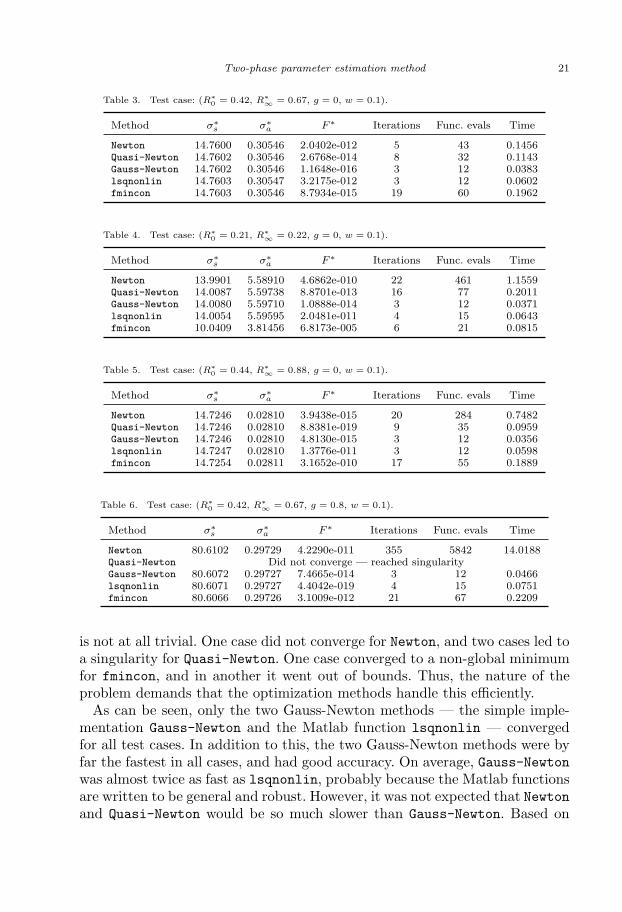
Two-phase parameter estimation method 21
Table 3. Test case: (R∗0 = 0.42, R∗
∞ = 0.67, g = 0, w = 0.1).
Method σ∗s σ∗
a F ∗ Iterations Func. evals Time
Newton 14.7600 0.30546 2.0402e-012 5 43 0.1456Quasi-Newton 14.7602 0.30546 2.6768e-014 8 32 0.1143Gauss-Newton 14.7602 0.30546 1.1648e-016 3 12 0.0383lsqnonlin 14.7603 0.30547 3.2175e-012 3 12 0.0602fmincon 14.7603 0.30546 8.7934e-015 19 60 0.1962
Table 4. Test case: (R∗0 = 0.21, R∗
∞ = 0.22, g = 0, w = 0.1).
Method σ∗s σ∗
a F ∗ Iterations Func. evals Time
Newton 13.9901 5.58910 4.6862e-010 22 461 1.1559Quasi-Newton 14.0087 5.59738 8.8701e-013 16 77 0.2011Gauss-Newton 14.0080 5.59710 1.0888e-014 3 12 0.0371lsqnonlin 14.0054 5.59595 2.0481e-011 4 15 0.0643fmincon 10.0409 3.81456 6.8173e-005 6 21 0.0815
Table 5. Test case: (R∗0 = 0.44, R∗
∞ = 0.88, g = 0, w = 0.1).
Method σ∗s σ∗
a F ∗ Iterations Func. evals Time
Newton 14.7246 0.02810 3.9438e-015 20 284 0.7482Quasi-Newton 14.7246 0.02810 8.8381e-019 9 35 0.0959Gauss-Newton 14.7246 0.02810 4.8130e-015 3 12 0.0356lsqnonlin 14.7247 0.02810 1.3776e-011 3 12 0.0598fmincon 14.7254 0.02811 3.1652e-010 17 55 0.1889
Table 6. Test case: (R∗0 = 0.42, R∗
∞ = 0.67, g = 0.8, w = 0.1).
Method σ∗s σ∗
a F ∗ Iterations Func. evals Time
Newton 80.6102 0.29729 4.2290e-011 355 5842 14.0188Quasi-Newton Did not converge — reached singularityGauss-Newton 80.6072 0.29727 7.4665e-014 3 12 0.0466lsqnonlin 80.6071 0.29727 4.4042e-019 4 15 0.0751fmincon 80.6066 0.29726 3.1009e-012 21 67 0.2209
is not at all trivial. One case did not converge for Newton, and two cases led toa singularity for Quasi-Newton. One case converged to a non-global minimumfor fmincon, and in another it went out of bounds. Thus, the nature of theproblem demands that the optimization methods handle this efficiently.
As can be seen, only the two Gauss-Newton methods — the simple imple-mentation Gauss-Newton and the Matlab function lsqnonlin — convergedfor all test cases. In addition to this, the two Gauss-Newton methods were byfar the fastest in all cases, and had good accuracy. On average, Gauss-Newtonwas almost twice as fast as lsqnonlin, probably because the Matlab functionsare written to be general and robust. However, it was not expected that Newtonand Quasi-Newton would be so much slower than Gauss-Newton. Based on
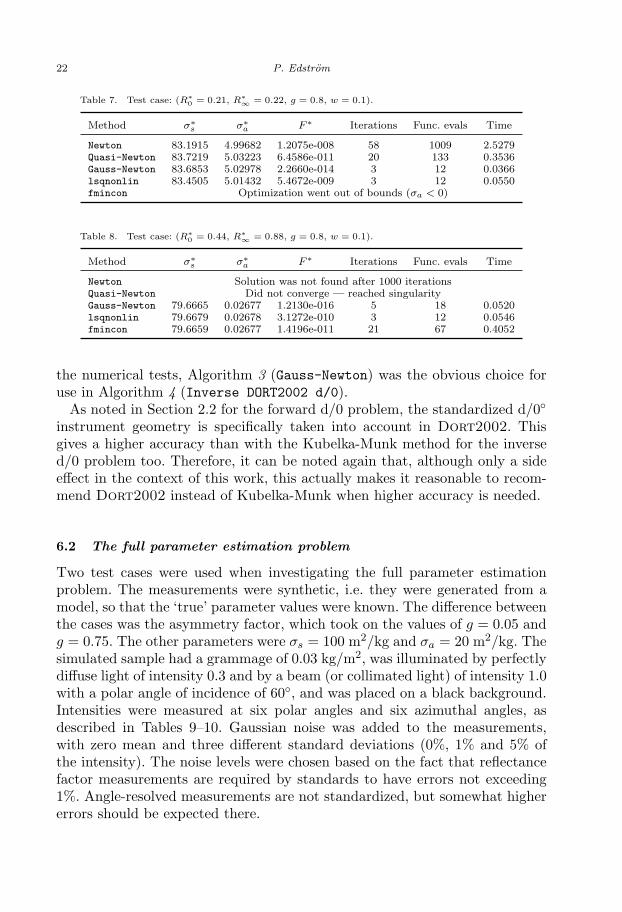
22 P. Edstrom
Table 7. Test case: (R∗0 = 0.21, R∗
∞ = 0.22, g = 0.8, w = 0.1).
Method σ∗s σ∗
a F ∗ Iterations Func. evals Time
Newton 83.1915 4.99682 1.2075e-008 58 1009 2.5279Quasi-Newton 83.7219 5.03223 6.4586e-011 20 133 0.3536Gauss-Newton 83.6853 5.02978 2.2660e-014 3 12 0.0366lsqnonlin 83.4505 5.01432 5.4672e-009 3 12 0.0550fmincon Optimization went out of bounds (σa < 0)
Table 8. Test case: (R∗0 = 0.44, R∗
∞ = 0.88, g = 0.8, w = 0.1).
Method σ∗s σ∗
a F ∗ Iterations Func. evals Time
Newton Solution was not found after 1000 iterationsQuasi-Newton Did not converge — reached singularityGauss-Newton 79.6665 0.02677 1.2130e-016 5 18 0.0520lsqnonlin 79.6679 0.02678 3.1272e-010 3 12 0.0546fmincon 79.6659 0.02677 1.4196e-011 21 67 0.4052
the numerical tests, Algorithm 3 (Gauss-Newton) was the obvious choice foruse in Algorithm 4 (Inverse DORT2002 d/0).
As noted in Section 2.2 for the forward d/0 problem, the standardized d/0◦instrument geometry is specifically taken into account in Dort2002. Thisgives a higher accuracy than with the Kubelka-Munk method for the inversed/0 problem too. Therefore, it can be noted again that, although only a sideeffect in the context of this work, this actually makes it reasonable to recom-mend Dort2002 instead of Kubelka-Munk when higher accuracy is needed.
6.2 The full parameter estimation problem
Two test cases were used when investigating the full parameter estimationproblem. The measurements were synthetic, i.e. they were generated from amodel, so that the ‘true’ parameter values were known. The difference betweenthe cases was the asymmetry factor, which took on the values of g = 0.05 andg = 0.75. The other parameters were σs = 100 m2/kg and σa = 20 m2/kg. Thesimulated sample had a grammage of 0.03 kg/m2, was illuminated by perfectlydiffuse light of intensity 0.3 and by a beam (or collimated light) of intensity 1.0with a polar angle of incidence of 60◦, and was placed on a black background.Intensities were measured at six polar angles and six azimuthal angles, asdescribed in Tables 9–10. Gaussian noise was added to the measurements,with zero mean and three different standard deviations (0%, 1% and 5% ofthe intensity). The noise levels were chosen based on the fact that reflectancefactor measurements are required by standards to have errors not exceeding1%. Angle-resolved measurements are not standardized, but somewhat highererrors should be expected there.
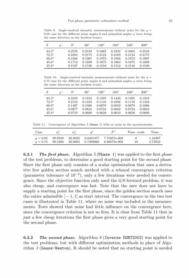
Two-phase parameter estimation method 23
Table 9. Angle-resolved intensity measurements without noise for the g =0.05 case for the different polar angles θ and azimuthal angles ϕ (zero beingthe same direction as the incident beam).
θ ϕ : 0◦ 60◦ 120◦ 180◦ 240◦ 300◦
84.3◦ 0.2576 0.2534 0.2462 0.2432 0.2462 0.253472.5◦ 0.2204 0.2175 0.2124 0.2103 0.2124 0.217560.0◦ 0.1928 0.1907 0.1872 0.1856 0.1872 0.190745.6◦ 0.1712 0.1699 0.1675 0.1664 0.1675 0.169925.8◦ 0.1537 0.1530 0.1518 0.1512 0.1518 0.1530
Table 10. Angle-resolved intensity measurements without noise for the g =0.75 case for the different polar angles θ and azimuthal angles ϕ (zero beingthe same direction as the incident beam).
θ ϕ : 0◦ 60◦ 120◦ 180◦ 240◦ 300◦
84.3◦ 0.3459 0.1918 0.1505 0.1440 0.1505 0.191872.5◦ 0.2152 0.1434 0.1116 0.1056 0.1116 0.143460.0◦ 0.1407 0.1086 0.0878 0.0832 0.0878 0.108645.6◦ 0.0977 0.0845 0.0724 0.0692 0.0724 0.084525.8◦ 0.0719 0.0680 0.0628 0.0610 0.0628 0.0680
Table 11. Convergence of Algorithm 5 (Phase 1) with no noise in the measurements.
Case σ∗s σ∗
a g∗ F ∗ Func. evals Time
g = 0.05 99.8949 20.0032 0.0491377 7.78257e-008 6 1.44267g = 0.75 99.5200 20.0003 0.7489060 6.86673e-008 10 2.73832
6.2.1 The first phase. Algorithm 5 (Phase 1) was applied to the first phaseof the test problems, to determine a good starting point for the second phase.Since the first phase only consists of a scalar optimization that uses a deriva-tive free golden section search method with a relaxed convergence criterion(parameter tolerance of 10−2), only a few iterations were needed for conver-gence. Since the objective function only used the d/0 forward problem, it wasalso cheap, and convergence was fast. Note that the user does not have tosupply a starting point for the first phase, since the golden section search usesthe entire admissible ]−1, 1[ as start interval. The convergence in the two testcases is illustrated in Table 11, where no noise was included in the measure-ments. Tests showed that noise had little influence on the convergence here,since the convergence criterion is not so firm. It is clear from Table 11 that injust a few cheap iterations the first phase gives a very good starting point forthe second phase.
6.2.2 The second phase. Algorithm 6 (Inverse DORT2002) was applied tothe test problems, but with different optimization methods in place of Algo-rithm 3 (Gauss-Newton). It should be noted that no starting point is needed
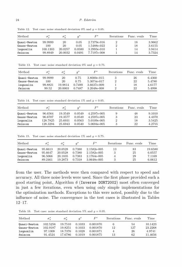
24 P. Edstrom
Table 12. Test case: noise standard deviation 0% and g = 0.05.
Method σ∗s σ∗
a g∗ F ∗ Iterations Func. evals Time
Quasi-Newton 99.9999 20 0.05 2.7379e-016 2 18 3.9662Gauss-Newton 100 20 0.05 1.5488e-022 2 18 3.6155lsqnonlin 100.1303 20.0257 0.0500 3.2993e-010 1 14 3.9414fmincon 99.8949 20.0032 0.0491 7.7197e-008 1 14 3.7324
Table 13. Test case: noise standard deviation 0% and g = 0.75.
Method σ∗s σ∗
a g∗ F ∗ Iterations Func. evals Time
Quasi-Newton 99.9999 20 0.75 3.8000e-015 3 26 6.4360Gauss-Newton 100 20 0.75 5.3074e-017 2 22 5.4780lsqnonlin 99.8821 19.9814 0.7499 3.6637e-009 1 18 4.6177fmincon 99.52 20.0003 0.7487 3.2048e-008 2 22 5.4998
Table 14. Test case: noise standard deviation 1% and g = 0.05.
Method σ∗s σ∗
a g∗ F ∗ Iterations Func. evals Time
Quasi-Newton 96.6564 19.3549 0.0549 4.2597e-005 9 48 9.1010Gauss-Newton 96.6707 19.3577 0.0549 4.2597e-005 3 23 4.4370lsqnonlin 128.7825 25.6931 0.0563 5.0109e-005 2 18 3.5425fmincon 128.3294 25.6943 0.0540 5.0694e-005 3 22 4.2755
Table 15. Test case: noise standard deviation 1% and g = 0.75.
Method σ∗s σ∗
a g∗ F ∗ Iterations Func. evals Time
Quasi-Newton 95.6613 20.0528 0.7380 2.1582e-005 13 83 19.6580Gauss-Newton 95.6647 20.0528 0.7380 2.1582e-005 3 25 6.0557lsqnonlin 96.5066 20.1835 0.7383 2.1764e-005 4 29 7.1169fmincon 89.2461 19.2873 0.7318 3.0648e-005 3 25 6.0612
from the user. The methods were then compared with respect to speed andaccuracy. All three noise levels were used. Since the first phase provided such agood starting point, Algorithm 6 (Inverse DORT2002) most often convergedin just a few iterations, even when using only simple implementations forthe optimization methods. Exceptions to this were noted, possibly due to theinfluence of noise. The convergence in the test cases is illustrated in Tables12–17.
Table 16. Test case: noise standard deviation 5% and g = 0.05.
Method σ∗s σ∗
a g∗ F ∗ Iterations Func. evals Time
Quasi-Newton 102.5256 19.7510 0.1033 0.001870 6 54 10.1423Gauss-Newton 102.9187 19.8251 0.1033 0.001870 12 127 23.2268lsqnonlin 97.1308 18.7376 0.1028 0.001871 4 26 4.9741fmincon 91.4524 17.6786 0.1019 0.001875 13 62 11.4656
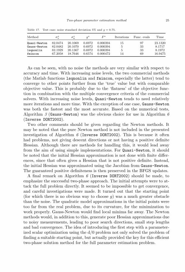
Two-phase parameter estimation method 25
Table 17. Test case: noise standard deviation 5% and g = 0.75.
Method σ∗s σ∗
a g∗ F ∗ Iterations Func. evals Time
Quasi-Newton 82.0474 20.1069 0.6972 0.000394 15 97 23.1320Gauss-Newton 82.0482 20.1070 0.6972 0.000394 5 33 8.1717lsqnonlin 82.1929 20.1367 0.6972 0.000394 5 33 8.1972fmincon 67.2058 18.7646 0.6574 0.000472 14 69 16.9475
As can be seen, with no noise the methods are very similar with respect toaccuracy and time. With increasing noise levels, the two commercial methods(the Matlab functions lsqnonlin and fmincon, especially the latter) tend toconverge to other points further from the ‘true’ value but with comparableobjective value. This is probably due to the ‘flatness’ of the objective func-tion in combination with the multiple convergence criteria of the commercialsolvers. With increasing noise levels, Quasi-Newton tends to need relativelymore iterations and more time. With the exception of one case, Gauss-Newtonwas both the fastest and the most accurate. Based on the numerical tests,Algorithm 3 (Gauss-Newton) was the obvious choice for use in Algorithm 6(Inverse DORT2002).
Two other comments should be given regarding the Newton methods. Itmay be noted that the pure Newton method is not included in the presentedinvestigation of Algorithm 6 (Inverse DORT2002). This is because it oftenhad problems, not giving descent directions or not having a positive definiteHessian. Although there are methods for handling this, it would lead awayfrom the aim of using simple implementations. For Quasi-Newton, it shouldbe noted that the initial Hessian approximation is not done with finite differ-ences, since that often gives a Hessian that is not positive definite. Instead,the initial Hessian was approximated using the Jacobian from Gauss-Newton.The guaranteed positive definiteness is then preserved in the BFGS updates.
A final remark on Algorithm 6 (Inverse DORT2002) should be made, toemphasize the successful two-phase approach. The initial attempts were to at-tack the full problem directly. It seemed to be impossible to get convergence,and careful investigations were made. It turned out that the starting point(for which there is no obvious way to choose g) was a much greater obstaclethan the noise. The quadratic model approximations in the initial points weretoo far from the real problem, due to its curvature, for the minimization towork properly. Gauss-Newton would find local minima far away. The Newtonmethods would, in addition to this, generate poor Hessian approximations dueto noisy measurements, leading to poor search directions, small step lengthsand bad convergence. The idea of introducing the first step with a parameter-ized scalar optimization using the d/0 problem not only solved the problem offinding a suitable starting point, but actually provided the key for this efficienttwo-phase solution method for the full parameter estimation problem.
26 P. Edstrom
It is appropriate to give a comment on the conditioning in the solution. Onaverage the condition number of the Hessian in the solution was 107, whichshows that the problem is indeed ill conditioned there. This can be comparedwith the d/0 problem, where the condition number was 2–3 decades smaller.This shows that although the d/0 problem also is ill conditioned in the solution,the introduction of the third parameter g in the parameter estimation problemincreased this ill-conditioning.
7 Discussion
Calculating material parameters from reflectance measurements is an out-standing issue in general radiative transfer problems. Finding a feasible start-ing point can in itself be a great problem in many applications. To the author’sknowledge the kind of two-phase approach for the inverse radiative transferproblem presented in this work has not been published before. It is not uncom-mon to first estimate σs and σa from some measurements and an assumptionor guess of g, and then use these parameter values as the starting point for thefull problem. However, this is far from optimal, since the values of σs and σa
are fixed from the more or less ad hoc choice of g. That first step merely ensuresthat the triplet σs, σa and g is compatible. No use is made of the full problemor the rest of the measurements when obtaining the starting point; instead, thestarting point and the rest of the problem are treated completely separately.The first phase suggested here manages to actually find the best (in some as-pect) starting point by actually combining — through the parameterization— the simpler d/0 problem with the objective function of the full problem,thus also utilizing all measurements. This intelligent construction of the firstphase made it fast and simple, while still providing a very good starting pointfor the full problem. The reported difficulties of finding a suitable startingpoint (for which the full problem is very sensitive) are thus eliminated, andthe user is relieved from having to supply an initial value of g through guess-work, and without knowledge. The starting point from the first phase thenmade it possible to use a simple and straightforward Gauss-Newton methodin the second phase, which gave fast convergence and accurate results. Thesuccessful recovery of σs, σa and g by this two-phase method was illustratedby application to relevant paper industry problems.
One goal of this work was simplicity in implementation. The numerical testsshow that this was indeed possible. The first phase is a simple golden sectionsearch method, and the second phase (as well as the d/0 case) is a simpleGauss-Newton method, both of which need no more than a few lines of code.The commercial solvers did not do any better, measuring any of convergence,final residual, iterations, function evaluations or computation time. The sim-
Two-phase parameter estimation method 27
ple Gauss-Newton method did as well as or better than all the other testedmethods, standard or commercial, in both the d/0 and full inverse problems.
Another purpose of this work was to find some characteristics of the stud-ied parameter estimation problem, since not much at all is known regardingexistence and uniqueness for the general radiative transfer problem and itsinverse. The investigations showed that the optimization problem is not at alltrivial, and that the nature of the ill-conditioned problem thus puts great de-mands on the optimization methods. It was also shown that higher opacity orhigher asymmetry factor increases the ill-conditioning, and that also estimat-ing the asymmetry factor (not only the scattering and absorption parameters)increases the condition number several decades. However, the relative sensitiv-ities found in the investigations are low, and should not be a problem in paperindustry applications. The type of analyses made in this work — using objec-tive function surface plots, phase space plots and sensitivity matrices — givegood insight into the character of the problem. Similar studies will be valuablein the design of instruments for angle-resolved measurements and in analysisof the corresponding measurement data. This will be particularly importantfor the paper industry, where anisotropy is gradually becoming an issue.
The Kubelka-Munk model is a simple solution method for the radiativetransfer problem, and it is well established in several industrial applicationsdue to its speed and ease of use. Its approximate solutions are sufficiently accu-rate in many applications, but there are a number of problems and applicationswhere higher accuracy is needed. This can be achieved with more general solu-tion methods for the radiative transfer problem, like Dort2002. To competewith Kubelka-Munk in industrial applications, higher accuracy is not enough.Sufficient speed is essential, as well as fast and accurate parameter estimationmethods. The specialized code for forward and inverse standardized d/0◦ re-flectance calculations reported in this work show that radiative transfer basedsolution methods like Dort2002 are now competitive in paper industry appli-cations. With its higher accuracy, larger range of applicability and comparablespeed, Dort2002 could well replace Kubelka-Munk in the paper industry forexample, for increased understanding. However, the Kubelka-Munk model willstill be useful in applications with lower demands on accuracy. When it is nowpossible to estimate the asymmetry factor g, the possibility of studying newmaterial phenomena such as different direction dependencies in reflectance andtransmittance arises. This opens up for increased understanding, but also forthe design of new paper and printed products.
28 P. Edstrom
8 Acknowledgements
This work was financially supported by T2F (‘TryckTeknisk Forskning’, aSwedish printing research program), which is gratefully acknowledged.
References[1] Kubelka, P. and Munk, F., 1931, Ein Beitrag zur Optik der Farbanstriche. Z. Tech. Phys., 11a,
593–601.[2] Kubelka, P., 1948, New contributions to the optics of intensely light-scattering materials. Part
I. J. Opt. Soc. Amer., 38, 448–457.[3] Kubelka, P., 1954, New Contributions to the optics of intensely light-scattering materials. Part
II. J. Opt. Soc. Amer., 44, 330–335.[4] Granberg, H. and Edstrom, P., 2003, Quantification of the Intrinsic Error of the Kubelka-Munk
Model Caused by Strong Light Absorption. J. Pulp Paper Sci, 29, 386–390.[5] Edstrom, P., 2004, Comparison of the DORT2002 Radiative Transfer Solution Method and the
Kubelka-Munk Model. Nordic Pulp Paper Res. J., 19, 397–403.[6] Neuman, M., 2005, Anisotropic Reflectance from Paper — Measurements, Simulations and Anal-
ysis. Master’s Thesis, Umea University, Sweden.[7] van Gemert, M. J. C. and Star, W. M., 1987, Relations between the Kubelka-Munk and the
Transport Equation Models for Anisotropic Scattering. Lasers Life Sci., 1, 287–298.[8] Prahl, S. A., van Gemert, M. J. C. and Welch, A. J., 1993, Determining the Optical Properties
of Turbid Media Using the Adding-Doubling Method. Appl. Opt., 32, 559–568.[9] Joshi, N., Donner, C. and Jensen, H. W., 2006, Noninvasive Measurement of Scattering
Anisotropy in Turbid Materials by Nonnormal Incident Illumination. Opt. Lett., 31, 936–938.[10] ISO 2469, 1994, Paper, board and pulps — Measurement of diffuse reflectance factor. Interna-
tional Organization for Standardization, Geneva, Switzerland.[11] ISO 2470, 1999, Paper, board and pulps — Measurement of diffuse blue reflectance factor (ISO
brightness). International Organization for Standardization, Geneva, Switzerland.[12] ISO 2471, 1998, Paper and board — Determination of opacity (paper backing) — Diffuse re-
flectance method. International Organization for Standardization, Geneva, Switzerland.[13] ISO 9416, 1998, Paper — Determination of light scattering and absorption coefficients (using
Kubelka-Munk theory). International Organization for Standardization, Geneva, Switzerland.[14] Edstrom, P., 2005, A Fast and Stable Solution Method for the Radiative Transfer Problem.
SIAM Rev., 47, 447–468.[15] Henyey, L. G. and Greenstein, J. L., 1941, Diffuse radiation in the galaxy. Astrophys. J., 93,
70–83.[16] Edstrom, P., 2007, Numerical Performance of Stability Enhancing and Speed Increasing Steps
in Radiative Transfer Solution Methods. Submitted to J. Comput. Appl. Math.[17] Armijo, L., 1966, Minimization of Functions Having Continuous Partial Derivatives. Pacific J.
Math., 16, 1–3.[18] Nash, S. G. and Sofer, A., 1999, Linear and Nonlinear Programming. (McGraw Hill, Singapore).[19] Bertsekas, D. P., 1999, Nonlinear Programming (2nd edn). (Athena Scientific, Belmont).[20] Broyden, C. G., 1970, The Convergence of a Class of Double-Rank Minimization Algorithms. J.
Inst. Math. Applic., 6, 76–90.[21] Fletcher, R., 1970, A New Approach to Variable Metric Algorithms. Computer J., 13, 317–322.[22] Goldfarb, D., 1970, A Family of Variable Metric Updates Derived by Variational Means. Math.
Comp., 24, 23–26.[23] Shanno, D. F., 1970, Conditioning of Quasi-Newton Methods for Function Minimization. Math.
Comp. , 24, 647–656.[24] More, J. J., 1977, The Levenberg-Marquardt Algorithm: Implementation and Theory. In G.
A. Watson (Ed) Numerical Analysis, Lecture Notes in Mathematics 630 (Springer Verlag), pp105–116.
[25] Schittkowski, K., 1985, NLQPL: A FORTRAN- Subroutine Solving Constrained Nonlinear Pro-gramming Problems. Ann. Oper. Res., 5, 485–500.
[26] Mudgett, P. S. and Richards, L. W., 1971, Multiple scattering calculations for technology. Appl.Opt., 10, 1485–1502.

Two-phase parameter estimation method 29
[27] Mudgett, P. S. and Richards, L. W., 1972, Multiple scattering calculations for technology II. J.Colloid Interf. Sci., 39, 551–567.
[28] H. C. van de Hulst, 1980, Multiple Light Scattering. Tables, Formulas and Applications. Vol. 2.(Academic Press, New York).


VII

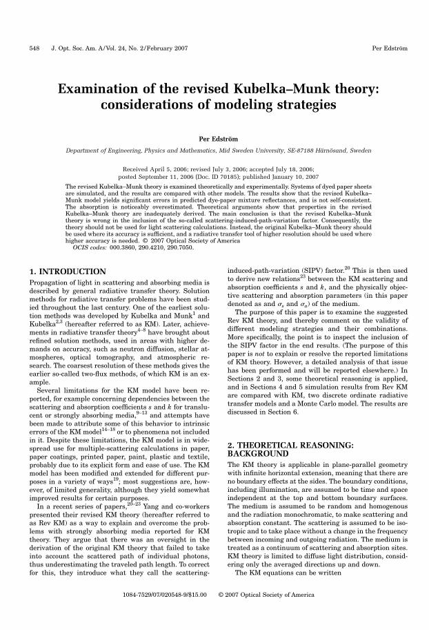
Examination of the revised Kubelka–Munk theory:considerations of modeling strategies
Per Edström
Department of Engineering, Physics and Mathematics, Mid Sweden University, SE-87188 Härnösand, Sweden
Received April 5, 2006; revised July 3, 2006; accepted July 18, 2006;posted September 11, 2006 (Doc. ID 70185); published January 10, 2007
The revised Kubelka–Munk theory is examined theoretically and experimentally. Systems of dyed paper sheetsare simulated, and the results are compared with other models. The results show that the revised Kubelka–Munk model yields significant errors in predicted dye-paper mixture reflectances, and is not self-consistent.The absorption is noticeably overestimated. Theoretical arguments show that properties in the revisedKubelka–Munk theory are inadequately derived. The main conclusion is that the revised Kubelka–Munktheory is wrong in the inclusion of the so-called scattering-induced-path-variation factor. Consequently, thetheory should not be used for light scattering calculations. Instead, the original Kubelka–Munk theory shouldbe used where its accuracy is sufficient, and a radiative transfer tool of higher resolution should be used wherehigher accuracy is needed. © 2007 Optical Society of America
OCIS codes: 000.3860, 290.4210, 290.7050.
1. INTRODUCTIONPropagation of light in scattering and absorbing media isdescribed by general radiative transfer theory. Solutionmethods for radiative transfer problems have been stud-ied throughout the last century. One of the earliest solu-tion methods was developed by Kubelka and Munk1 andKubelka2,3 (hereafter referred to as KM). Later, achieve-ments in radiative transfer theory4–8 have brought aboutrefined solution methods, used in areas with higher de-mands on accuracy, such as neutron diffusion, stellar at-mospheres, optical tomography, and atmospheric re-search. The coarsest resolution of these methods gives theearlier so-called two-flux methods, of which KM is an ex-ample.
Several limitations for the KM model have been re-ported, for example concerning dependencies between thescattering and absorption coefficients s and k for translu-cent or strongly absorbing media,9–13 and attempts havebeen made to attribute some of this behavior to intrinsicerrors of the KM model14–18 or to phenomena not includedin it. Despite these limitations, the KM model is in wide-spread use for multiple-scattering calculations in paper,paper coatings, printed paper, paint, plastic and textile,probably due to its explicit form and ease of use. The KMmodel has been modified and extended for different pur-poses in a variety of ways19; most suggestions are, how-ever, of limited generality, although they yield somewhatimproved results for certain purposes.
In a recent series of papers,20–23 Yang and co-workerspresented their revised KM theory (hereafter referred toas Rev KM) as a way to explain and overcome the prob-lems with strongly absorbing media reported for KMtheory. They argue that there was an oversight in thederivation of the original KM theory that failed to takeinto account the scattered path of individual photons,thus underestimating the traveled path length. To correctfor this, they introduce what they call the scattering-
induced-path-variation (SIPV) factor.20 This is then usedto derive new relations23 between the KM scattering andabsorption coefficients s and k, and the physically objec-tive scattering and absorption parameters (in this paperdenoted as and �s and �a) of the medium.
The purpose of this paper is to examine the suggestedRev KM theory, and thereby comment on the validity ofdifferent modeling strategies and their combinations.More specifically, the point is to inspect the inclusion ofthe SIPV factor in the end results. (The purpose of thispaper is not to explain or resolve the reported limitationsof KM theory. However, a detailed analysis of that issuehas been performed and will be reported elsewhere.) InSections 2 and 3, some theoretical reasoning is applied,and in Sections 4 and 5 simulation results from Rev KMare compared with KM, two discrete ordinate radiativetransfer models and a Monte Carlo model. The results arediscussed in Section 6.
2. THEORETICAL REASONING:BACKGROUNDThe KM theory is applicable in plane-parallel geometrywith infinite horizontal extension, meaning that there areno boundary effects at the sides. The boundary conditions,including illumination, are assumed to be time and spaceindependent at the top and bottom boundary surfaces.The medium is assumed to be random and homogenousand the radiation monochromatic, to make scattering andabsorption constant. The scattering is assumed to be iso-tropic and to take place without a change in the frequencybetween incoming and outgoing radiation. The medium istreated as a continuum of scattering and absorption sites.KM theory is limited to diffuse light distribution, consid-ering only the averaged directions up and down.
The KM equations can be written
548 J. Opt. Soc. Am. A/Vol. 24, No. 2 /February 2007 Per Edström
1084-7529/07/020548-9/$15.00 © 2007 Optical Society of America
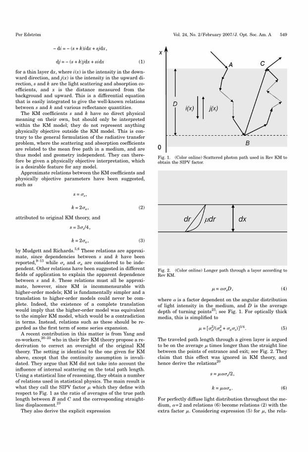
− di = − �s + k�idx + sjdx,
dj = − �s + k�jdx + sidx �1�
for a thin layer dx, where i�x� is the intensity in the down-ward direction, and j�x� is the intensity in the upward di-rection, s and k are the light scattering and absorption co-efficients, and x is the distance measured from thebackground and upward. This is a differential equationthat is easily integrated to give the well-known relationsbetween s and k and various reflectance quantities.
The KM coefficients s and k have no direct physicalmeaning on their own, but should only be interpretedwithin the KM model; they do not represent anythingphysically objective outside the KM model. This is con-trary to the general formulation of the radiative transferproblem, where the scattering and absorption coefficientsare related to the mean free path in a medium, and arethus model and geometry independent. They can there-fore be given a physically objective interpretation, whichis a desirable feature for any model.
Approximate relations between the KM coefficients andphysically objective parameters have been suggested,such as
s = �s,
k = 2�a, �2�
attributed to original KM theory, and
s = 3�s/4,
k = 2�a, �3�
by Mudgett and Richards.5,6 These relations are approxi-mate, since dependencies between s and k have beenreported,9–13 while �s and �a are considered to be inde-pendent. Other relations have been suggested in differentfields of application to explain the apparent dependencebetween s and k. These relations must all be approxi-mate, however, since KM is incommensurable withhigher-order models; KM is fundamentally simpler and atranslation to higher-order models could never be com-plete. Indeed, the existence of a complete translationwould imply that the higher-order model was equivalentto the simpler KM model, which would be a contradictionin terms. Instead, relations such as these should be re-garded as the first term of some series expansion.
A recent contribution in this matter is from Yang andco-workers,20–23 who in their Rev KM theory propose a re-derivation to correct an oversight of the original KMtheory. The setting is identical to the one given for KMabove, except that the continuity assumption is invali-dated. They argue that KM did not take into account theinfluence of internal scattering on the total path length.Using a statistical line of reasoning, they obtain a numberof relations used in statistical physics. The main result iswhat they call the SIPV factor � which they define withrespect to Fig. 1 as the ratio of averages of the true pathlength between B and C and the corresponding straight-line displacement.23
They also derive the explicit expression
� = ��sD, �4�
where � is a factor dependent on the angular distributionof light intensity in the medium, and D is the averagedepth of turning points23; see Fig. 1. For optically thickmedia, this is simplified to
� = ��s2/��a
2 + �a�s��1/4. �5�
The traveled path length through a given layer is arguedto be on the average � times longer than the straight linebetween the points of entrance and exit; see Fig. 2. Theyclaim that this effect was ignored in KM theory, andhence derive the relations20
s = ���s/2,
k = ���a. �6�
For perfectly diffuse light distribution throughout the me-dium, �=2 and relations (6) become relations (2) with theextra factor �. Considering expression (5) for �, the rela-
Fig. 1. (Color online) Scattered photon path used in Rev KM toobtain the SIPV factor.
Fig. 2. (Color online) Longer path through a layer according toRev KM.
Per Edström Vol. 24, No. 2 /February 2007/J. Opt. Soc. Am. A 549
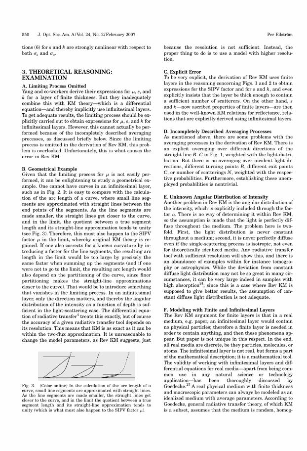
tions (6) for s and k are strongly nonlinear with respect toboth �s and �a.
3. THEORETICAL REASONING:EXAMINATIONA. Limiting Process OmittedYang and co-workers derive their expressions for �, s, andk for a layer of finite thickness. But they inadequatelycombine this with KM theory—which is a differentialequation—and thereby implicitly use infinitesimal layers.To get adequate results, the limiting process should be ex-plicitly carried out to obtain expressions for �, s, and k forinfinitesimal layers. However, this cannot actually be per-formed because of the incompletely described averagingprocesses, as discussed briefly below. Since the limitingprocess is omitted in the derivation of Rev KM, this prob-lem is overlooked. Unfortunately, this is what causes theerror in Rev KM.
B. Geometrical ExampleGiven that the limiting process for � is not easily per-formed, it can be enlightening to study a geometrical ex-ample. One cannot have curves in an infinitesimal layer,such as in Fig. 2. It is easy to compare with the calcula-tion of the arc length of a curve, where small line seg-ments are approximated with straight lines between theend points of the segments. As the line segments aremade smaller, the straight lines get closer to the curve,and in the limit, the quotient between a true segmentlength and its straight-line approximation tends to unity(see Fig. 3). Therefore, this must also happen to the SIPVfactor � in the limit, whereby original KM theory is re-gained. If one also corrects for a known curvature by in-troducing a factor for the line segments, the resulting arclength in the limit would be too large by precisely thesame factor when summing up the segments (and if onewere not to go to the limit, the resulting arc length wouldalso depend on the partitioning of the curve, since finerpartitioning makes the straight-line approximationscloser to the curve). That would be to introduce somethingthat vanishes in the limiting process. In an infinitesimallayer, only the direction matters, and thereby the angulardistribution of the intensity as a function of depth is suf-ficient in the light-scattering case. The differential equa-tion of radiative transfer4 treats this exactly, but of coursethe accuracy of a given radiative transfer tool depends onits resolution. This means that KM is as exact as it can bewithin the two-flux approximation. It is unreasonable tochange the model parameters, as Rev KM suggests, just
because the resolution is not sufficient. Instead, theproper thing to do is to use a model with higher resolu-tion.
C. Explicit ErrorTo be very explicit, the derivation of Rev KM uses finitelayers in the reasoning concerning Figs. 1 and 2 to obtainexpressions for the SIPV factor and for s and k, and evenexplicitly insists that the layer be thick enough to containa sufficient number of scatterers. On the other hand, sand k—now ascribed properties of finite layers—are thenused in the well-known KM relations for reflectance, rela-tions that are explicitly derived using infinitesimal layers.
D. Incompletely Described Averaging ProcessesAs mentioned above, there are some problems with theaveraging processes in the derivation of Rev KM. There isan explicit averaging over different directions of thestraight line B–C in Fig. 1, weighted with the light distri-bution. But there is no averaging over incident light di-rections, different turning points B, different exit pointsC, or number of scatterings N, weighted with the respec-tive probabilities. Furthermore, establishing these unem-ployed probabilities is nontrivial.
E. Unknown Angular Distribution of IntensityAnother problem in Rev KM is the angular distribution ofthe intensity, which is explicitly included through the fac-tor �. There is no way of determining it within Rev KM,so the assumption is made that the light is perfectly dif-fuse throughout the medium. The problem here is two-fold. First, the light distribution is never constantthroughout a medium; second, it is never perfectly diffuseeven if the single-scattering process is isotropic, not evenfor theoretically idealized media. Any radiative transfertool with sufficient resolution will show this, and there isan abundance of examples within for instance tomogra-phy or astrophysics. While the deviation from constantdiffuse light distribution may not be so great in many cir-cumstances, it can be very large indeed in samples withhigh absorption24; since this is a case where Rev KM issupposed to give better results, the assumption of con-stant diffuse light distribution is not adequate.
F. Modeling with Finite and Infinitesimal LayersThe Rev KM argument for finite layers is that in a realmedium, e.g. paper, an infinitesimal layer would containno physical particles; therefore a finite layer is needed inorder to contain anything, and then these phenomena ap-pear. But paper is not unique in this respect. In the end,all real media are discrete, be they particles, molecules, oratoms. The infinitesimal layer is not real, but forms a partof the mathematical description; it is a mathematical tool.The validity of working with infinitesimal layers and dif-ferential equations for real media—apart from being com-mon use in any natural science or technologyapplication—has been thoroughly discussed byGoedecke.25 A real physical medium with finite thicknessand macroscopic parameters can always be modeled as anidealized medium with average parameters. According toGoedecke, general radiative transfer theory, of which KMis a subset, assumes that the medium is random, homog-
Fig. 3. (Color online) In the calculation of the arc length of acurve, small line segments are approximated with straight lines.As the line segments are made smaller, the straight lines getcloser to the curve, and in the limit the quotient between a truesegment length and its straight-line approximation tends tounity (which is what must also happen to the SIPV factor �).
550 J. Opt. Soc. Am. A/Vol. 24, No. 2 /February 2007 Per Edström
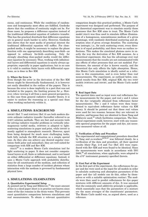
enous, and continuous. While the conditions of random-ness and homogeneity most often are fulfilled, Goedeckeshows that the condition of continuity might not be. Forthose cases, he proposes a difference equation instead ofthe traditional differential equation of radiative transfer.This has the practical drawback that difference equationsare in general much harder to solve. However, Goedeckealso shows that for most media of practical interest thetraditional differential equation will suffice. For close-packed media, it might be necessary to replace the phasefunction with one appropriately describing near-field—asopposed to ordinary far-field—scattering. Only forstrongly absorbing close-packed media would the differ-ence equation be necessary. Thus, working with infinitesi-mal layers and differential equations is nearly always ap-propriate, especially in paper applications, but in no caseis it valid to combine finite layers with differential equa-tions, as is done in Rev KM.
G. Where the Error IsEven though the error in the derivation of the Rev KMtheory might be theoretically fundamental, it is howevernot easily identified in the outline of the papers. This isbecause the error is done implicitly in a part that was notincluded in the papers, the limiting process for �. How-ever, when viewing it all from a more general perspective,in this case from general radiative transfer theory, it iseasier to analyze the reasoning as a special case thanwhen working exclusively within it.
4. SIMULATIONS: BACKGROUNDDISORT (Ref. 7) and DORT2002 (Ref. 8) are both modern dis-crete ordinate radiative transfer (hereafter referred to asDORT) solution methods. They are fast and accurate toolsfor solving radiative transfer problems in vertically inho-mogeneous turbid media. DORT2002 is adapted to light-scattering simulations in paper and print, while DISORT ismostly applied to atmospheric research. However, apartfrom being designed for much more challenging tasks,both fully include the KM situation as a simple specialcase. As they also can achieve any desired angular reso-lution (both polar and azimuthal), they are well suited forcomparison with KM and Rev KM.
GRACE26 is a modern Monte Carlo simulation tool forlight scattering in paper. It does not consider computa-tional layers at all, finite or infinitesimal, and is not basedon either differential or difference equations. Instead, ituses a Monte Carlo approach with probability distribu-tions for all constituents of the medium, and collection ofstatistics from a large number of incident photons whoseinteraction with the medium is governed by fundamentalphysical laws.
5. SIMULATIONS: EXAMINATIONA. Quantitative Experimental SetupAs pointed out by Yang and Miklavcic,23 the exact amountof dye in a dyed paper sheet is in practice not known sincesome of the dye remains in the drain water. This preventsexact quantitative comparison between simulations andreal measurements. To obtain a relevant quantitative
comparison despite this practical problem, a Monte Carloexperiment was designed and performed. The purpose ofthe theoretical experiment was to simulate exactly thoseprocesses that Rev KM aims to treat. The Monte Carlomodel GRACE was thus used to simulate diffuse illumina-tion of a homogenous, noncontinuous medium of a givengrammage, with randomly distributed scattering and ab-sorption sites of given average densities. The scatteringwas isotropic; i.e., for each scattering event, every direc-tion is of equal probability, and there were no surface re-flections. This makes the simulated photons move in ex-actly the way the derivation of Rev KM assumes. As atheoretical experiment, this has the advantage over realmeasurements that the results are not contaminated withany effects of other processes that are not modeled. Fur-thermore, the amount of dye is known exactly, and thetheoretical dye only affects the light absorption. Hence,this Monte Carlo simulation is ideally suited as a refer-ence in this examination, and is even better than realmeasurements. The experiment, as outlined below, com-pared results from Rev KM, original KM, the two DORT
models DORT2002 and DISORT, and the Monte Carlo modelGRACE.
B. Real Input DataThe spectral data used as input were real reflectance fac-tor measurements for the paper, and real s and k valuesfor the dye (originally obtained from reflectance factormeasurements). The s and k values were then trans-formed to equivalent reflectance factor values via KMtheory. It should be pointed out that these real valueswere used for two reasons: because they are relevant inpractice, and because they are identical to those Yang andMiklavcic used,23 which facilitates comparison. The theo-retical experiment could, however, start with any reason-able spectral properties for the paper and dye, not neces-sary measured values at all.
C. Verification of Data and ProcedureThe experimental and computational procedure describedby Yang and co-workers20,23,27 was followed closely. As averification of the data and procedure, all their spectralresults [their Figs. 2–6 and 7(a) (Ref. 23)] were repro-duced with Rev KM and were found to be identical. Sincethe measurements were made in accordance with ISO2469,28 all simulations, when applicable, were adapted tothe d /0° instrument geometry specified therein.
D. First Part of the ExperimentIn the first part of the experiment, the reflectances for pa-per and dye were used as the input for all models in orderto calculate scattering and absorption parameters of thepaper and dye (all models can do this, either by them-selves or with a suitable optimization routine). The mod-els were then used to predict reflectances for dye–papermixtures with different amounts of dye. It was assumedthat the commonly used additivity principle is applicable,which essentially says that the parameters of a mixtureare the mass averages of the constituents’ parameters.The Monte Carlo model was, as argued above, used as areference.
Per Edström Vol. 24, No. 2 /February 2007/J. Opt. Soc. Am. A 551
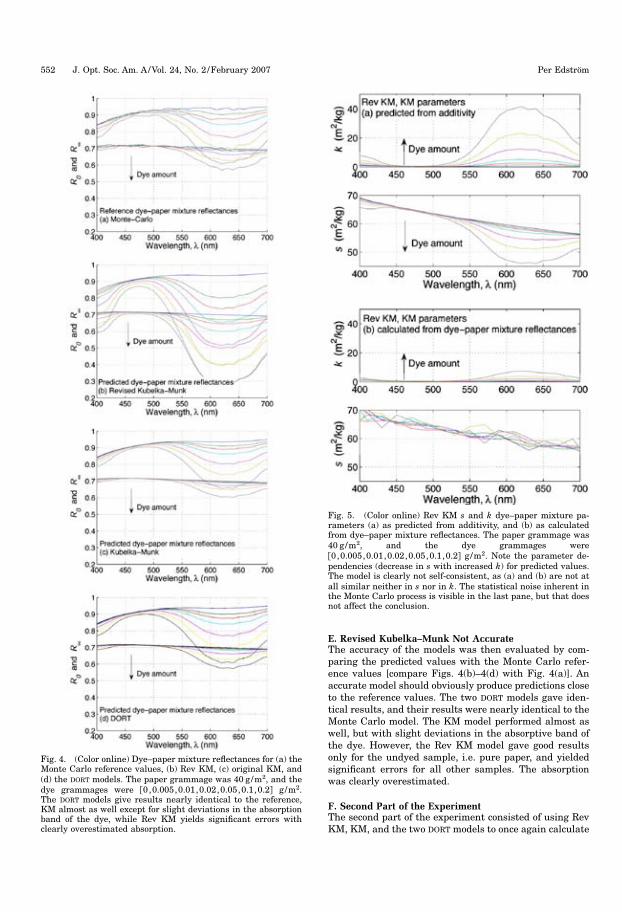
E. Revised Kubelka–Munk Not AccurateThe accuracy of the models was then evaluated by com-paring the predicted values with the Monte Carlo refer-ence values [compare Figs. 4(b)–4(d) with Fig. 4(a)]. Anaccurate model should obviously produce predictions closeto the reference values. The two DORT models gave iden-tical results, and their results were nearly identical to theMonte Carlo model. The KM model performed almost aswell, but with slight deviations in the absorptive band ofthe dye. However, the Rev KM model gave good resultsonly for the undyed sample, i.e. pure paper, and yieldedsignificant errors for all other samples. The absorptionwas clearly overestimated.
F. Second Part of the ExperimentThe second part of the experiment consisted of using RevKM, KM, and the two DORT models to once again calculate
Fig. 4. (Color online) Dye–paper mixture reflectances for (a) theMonte Carlo reference values, (b) Rev KM, (c) original KM, and(d) the DORT models. The paper grammage was 40 g/m2, and thedye grammages were �0,0.005,0.01,0.02,0.05,0.1,0.2� g/m2.The DORT models give results nearly identical to the reference,KM almost as well except for slight deviations in the absorptionband of the dye, while Rev KM yields significant errors withclearly overestimated absorption.
Fig. 5. (Color online) Rev KM s and k dye–paper mixture pa-rameters (a) as predicted from additivity, and (b) as calculatedfrom dye–paper mixture reflectances. The paper grammage was40 g/m2, and the dye grammages were�0,0.005,0.01,0.02,0.05,0.1,0.2� g/m2. Note the parameter de-pendencies (decrease in s with increased k) for predicted values.The model is clearly not self-consistent, as (a) and (b) are not atall similar neither in s nor in k. The statistical noise inherent inthe Monte Carlo process is visible in the last pane, but that doesnot affect the conclusion.
552 J. Opt. Soc. Am. A/Vol. 24, No. 2 /February 2007 Per Edström
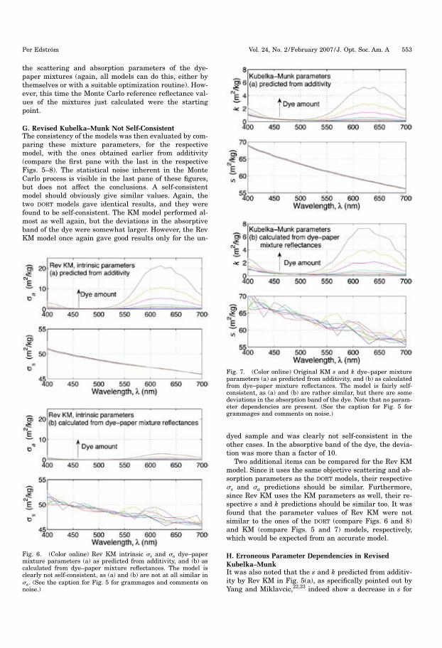
the scattering and absorption parameters of the dye-paper mixtures (again, all models can do this, either bythemselves or with a suitable optimization routine). How-ever, this time the Monte Carlo reference reflectance val-ues of the mixtures just calculated were the startingpoint.
G. Revised Kubelka–Munk Not Self-ConsistentThe consistency of the models was then evaluated by com-paring these mixture parameters, for the respectivemodel, with the ones obtained earlier from additivity(compare the first pane with the last in the respectiveFigs. 5–8). The statistical noise inherent in the MonteCarlo process is visible in the last pane of these figures,but does not affect the conclusions. A self-consistentmodel should obviously give similar values. Again, thetwo DORT models gave identical results, and they werefound to be self-consistent. The KM model performed al-most as well again, but the deviations in the absorptiveband of the dye were somewhat larger. However, the RevKM model once again gave good results only for the un-
dyed sample and was clearly not self-consistent in theother cases. In the absorptive band of the dye, the devia-tion was more than a factor of 10.
Two additional items can be compared for the Rev KMmodel. Since it uses the same objective scattering and ab-sorption parameters as the DORT models, their respective�s and �a predictions should be similar. Furthermore,since Rev KM uses the KM parameters as well, their re-spective s and k predictions should be similar too. It wasfound that the parameter values of Rev KM were notsimilar to the ones of the DORT (compare Figs. 6 and 8)and KM (compare Figs. 5 and 7) models, respectively,which would be expected from an accurate model.
H. Erroneous Parameter Dependencies in RevisedKubelka–MunkIt was also noted that the s and k predicted from additiv-ity by Rev KM in Fig. 5(a), as specifically pointed out byYang and Miklavcic,22,23 indeed show a decrease in s for
Fig. 6. (Color online) Rev KM intrinsic �s and �a dye–papermixture parameters (a) as predicted from additivity, and (b) ascalculated from dye–paper mixture reflectances. The model isclearly not self-consistent, as (a) and (b) are not at all similar in�a. (See the caption for Fig. 5 for grammages and comments onnoise.)
Fig. 7. (Color online) Original KM s and k dye–paper mixtureparameters (a) as predicted from additivity, and (b) as calculatedfrom dye–paper mixture reflectances. The model is fairly self-consistent, as (a) and (b) are rather similar, but there are somedeviations in the absorption band of the dye. Note that no param-eter dependencies are present. (See the caption for Fig. 5 forgrammages and comments on noise.)
Per Edström Vol. 24, No. 2 /February 2007 /J. Opt. Soc. Am. A 553
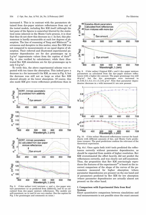
increased k. This is in contrast with the parameters ob-tained from dye-paper mixture reflectances from any ofthe tested models, including Rev KM itself (although thelast pane of the figures is somewhat blurred by the statis-tical noise inherent in the Monte Carlo process, it is clearthat they do not show this decrease in s). In fact, this phe-nomenon is hardly measurable at such low degrees of ab-sorption. The line of reasoning of Yang and Miklavcic23 iserroneous and deceptive in this matter, since Rev KM wasnot compared to measurements at an equal degree of ab-sorption. Their referred and illustrated experimental pa-rameter dependencies are for dye grammages up to2 g/m2 (approximate values from the caption of their23
Fig. 4, also verified by calculations), while their illus-trated Rev KM simulations are for dye grammages up toonly 0.2 g/m2.
To verify this, the above experimental scheme was re-peated with ten times the absorption. This indeed gave adecrease in s for increased k for KM, as seen in Fig. 9, butthe decrease was still not as large as what Rev KMshowed already at the lower absorption. Of course, thisalso made KM give worse reflectance predictions than in
Fig. 4(c). Once again both DORT tools predicted the reflec-tances correctly without parameter dependencies, asshould be expected from models of higher resolution. RevKM overestimated the effect heavily, did not predict thereflectances correctly, and was clearly not self-consistent.Thus, the proposition that Rev KM convincingly repro-duces the features of the experiments23 is based on the in-correct comparison of the shape of the curves of the pa-rameters measured for higher absorption (whereparameter dependencies are present) on the one hand andof parameters predicted by Rev KM for low absorption(where parameter dependencies are actually almost notpresent) on the other hand.
I. Comparison with Experimental Data from RealSystemsExact quantitative comparison between simulations andreal measurements is not possible since the exact amount
Fig. 8. (Color online) DORT intrinsic �s and �a dye–paper mix-ture parameters (a) as predicted from additivity, and (b) as cal-culated from dye–paper mixture reflectances. The models areself-consistent, as (a) and (b) are very similar. (See the caption forFig. 5 for grammages and comments on noise.)
Fig. 9. (Color online) Original KM s and k dye–paper mixtureparameters as calculated from the dye–paper mixture reflec-tances with a higher dye amount. The paper grammage was still40 g/m2, but the dye grammages were increased to�0,0.02,0.1,0.2,1.0,1.5,2.0� g/m2. Note that parameter depen-dencies (decrease in s with increased k) are now present.
Fig. 10. (Color online) Measured reflectances (curves) for hand-sheets with different amounts of dye, and Monte Carlo predic-tions (crosses). The good predictions confirm the relevance of thetheoretical experiment.
554 J. Opt. Soc. Am. A/Vol. 24, No. 2 /February 2007 Per Edström
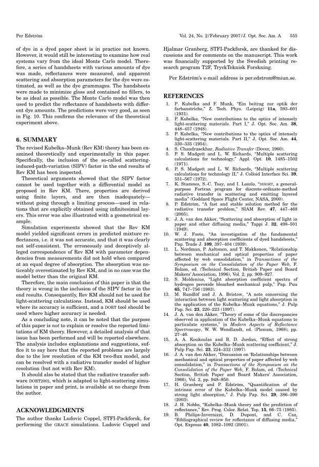
of dye in a dyed paper sheet is in practice not known.However, it would still be interesting to examine how realsystems vary from the ideal Monte Carlo model. There-fore, a series of handsheets with various amounts of dyewas made, reflectances were measured, and apparentscattering and absorption parameters for the dye were es-timated, as well as the dye grammages. The handsheetswere made to minimize gloss and contained no fillers, tobe as ideal as possible. The Monte Carlo model was thenused to predict the reflectance of handsheets with differ-ent dye amounts. The predictions were very good, as seenin Fig. 10. This confirms the relevance of the theoreticalexperiment above.
6. SUMMARYThe revised Kubelka–Munk (Rev KM) theory has been ex-amined theoretically and experimentally in this paper.Specifically, the inclusion of the so-called scattering-induced-path-variation (SIPV) factor in the end results ofRev KM has been inspected.
Theoretical arguments showed that the SIPV factorcannot be used together with a differential model asproposed in Rev KM. There, properties are derivedusing finite layers, and are then inadequately—without going through a limiting process—used in rela-tions that are explicitly obtained using infinitesimal lay-ers. This error was also illustrated with a geometrical ex-ample.
Simulation experiments showed that the Rev KMmodel yielded significant errors in predicted mixture re-flectances, i.e. it was not accurate, and that it was clearlynot self-consistent. The erroneously and deceptively al-leged correspondence of Rev KM with parameter depen-dencies from measurements did not hold when comparedat an equal degree of absorption. The absorption was no-ticeably overestimated by Rev KM, and in no case was themodel better than the original KM.
Therefore, the main conclusion of this paper is that thetheory is wrong in the inclusion of the SIPV factor in theend results. Consequently, Rev KM should not be used forlight-scattering calculations. Instead, KM should be usedwhere its accuracy is sufficient, and a DORT tool should beused where higher accuracy is needed.
As a concluding note, it can be noted that the purposeof this paper is not to explain or resolve the reported limi-tations of KM theory. However, a detailed analysis of thatissue has been performed and will be reported elsewhere.The analysis includes explanations and suggestions, suf-fice it to say here that the reported problems are largelydue to the low resolution of the KM two-flux model, andcan be resolved with a radiative transfer model of higherresolution (but not with Rev KM).
It should also be stated that the radiative transfer soft-ware DORT2002, which is adapted to light-scattering simu-lations in paper and print, is available at no charge fromthe author.
ACKNOWLEDGMENTSThe author thanks Ludovic Coppel, STFI-Packforsk, forperforming the GRACE simulations. Ludovic Coppel and
Hjalmar Granberg, STFI-Packforsk, are thanked for dis-cussions and for comments on the manuscript. This workwas financially supported by the Swedish printing re-search program T2F, TryckTeknisk Forskning.
Per Edström’s e-mail address is [email protected].
REFERENCES1. P. Kubelka and F. Munk, “Ein beitrag zur optik der
farbanstriche,” Z. Tech. Phys. (Leipzig) 11a, 593–601(1931).
2. P. Kubelka, “New contributions to the optics of intenselylight-scattering materials. Part I,” J. Opt. Soc. Am. 38,448–457 (1948).
3. P. Kubelka, “New contributions to the optics of intenselylight-scattering materials. Part II,” J. Opt. Soc. Am. 44,330–335 (1954).
4. S. Chandrasekhar, Radiative Transfer (Dover, 1960).5. P. S. Mudgett and L. W. Richards, “Multiple scattering
calculations for technology,” Appl. Opt. 10, 1485–1502(1971).
6. P. S. Mudgett and L. W. Richards, “Multiple scatteringcalculations for technology II,” J. Colloid Interface Sci. 39,551–567 (1972).
7. K. Stamnes, S.-C. Tsay, and I. Laszlo, “DISORT, a general-purpose Fortran program for discrete-ordinate-methodradiative transfer in scattering and emitting layeredmedia” (Goddard Space Flight Center, NASA, 2000).
8. P. Edström, “A fast and stable solution method for theradiative transfer problem,” SIAM Rev. 47, 447–468(2005).
9. J. A. van den Akker, “Scattering and absorption of light inpaper and other diffusing media,” Tappi J. 32, 498–501(1949).
10. W. J. Foote, “An investigation of the fundamentalscattering and absorption coefficients of dyed handsheets,”Pap. Trade J. 109, 397–404 (1939).
11. L. Nordman, P. Aaltonen, and T. Makkonen, “Relationshipbetween mechanical and optical properties of paperaffected by web consolidation,” in Transactions of theSymposium on the Consolidation of the Paper Web, F.Bolam, ed. (Technical Section, British Paper and BoardMakers’ Association, 1996), Vol. 2, pp. 909–927.
12. S. Moldenius, “Light absorption coefficient spectra ofhydrogen peroxide bleached mechanical pulp,” Pap. Puu65, 747–756 (1983).
13. M. Rundlöf and J. A. Bristow, “A note concerning theinteraction between light scattering and light absorption inthe application of the Kubelka–Munk equations,” J. PulpPap. Sci. 23, 220–223 (1997).
14. J. A. van den Akker, “Theory of some of the discrepanciesobserved in application of the Kubelka–Munk equations toparticulate systems,” in Modern Aspects of ReflectanceSpectroscopy, W. W. Wendlandt, ed. (Plenum, 1968), pp.27–46.
15. A. A. Koukoulas and B. D. Jordan, “Effect of strongabsorption on the Kubelka–Munk scattering coefficient,” J.Pulp Pap. Sci. 23, 224–232 (1997).
16. J. A. van den Akker, “Discussion on ‘Relationships betweenmechanical and optical properties of paper affected by webconsolidation,” in Transactions of the Symposium on theConsolidation of the Paper Web, F. Bolam, ed. (TechnicalSection, British Paper and Board Makers’ Association,1966), Vol. 2, pp. 948–950.
17. H. Granberg and P. Edström, “Quantification of theintrinsic error of the Kubelka–Munk model caused bystrong light absorption,” J. Pulp Pap. Sci. 29, 386–390(2003).
18. J. H. Nobbs, “Kubelka–Munk theory and the prediction ofreflectance,” Rev. Prog. Color. Relat. Top. 15, 66–75 (1985).
19. B. Philips-Invernizzi, D. Dupont, and C. Caz,“Bibliographical review for reflectance of diffusing media,”Opt. Express 40, 1082–1092 (2001).
Per Edström Vol. 24, No. 2 /February 2007/J. Opt. Soc. Am. A 555

20. L. Yang and B. Kruse, “Revised Kubelka–Munk theory. I.Theory and applications,” J. Opt. Soc. Am. A 21, 1933–1941(2004).
21. L. Yang, B. Kruse, and S. J. Miklavcic, “RevisedKubelka–Munk theory. II. Unified framework forhomogenous and inhomogenous optical media,” J. Opt. Soc.Am. A 21, 1942–1952 (2004).
22. L. Yang and S. J. Miklavcic, “A theory of light propagationincorporating scattering and absorption in turbid media,”Opt. Lett. 30, 792–794 (2005).
23. L. Yang and S. J. Miklavcic, “Revised Kubelka–Munktheory. III. A general theory of light propagation inscattering and absorptive media,” J. Opt. Soc. Am. A 22,1866–1873 (2005).
24. P. Edström, “Comparison of the DORT2002 radiative transfer
solution method and the Kubelka–Munk model,” Nord.Pulp Pap. Res. J. 19, 397–403 (2004).
25. G. H. Goedecke, “Radiative transfer in closely packedmedia,” J. Opt. Soc. Am. 67, 1339–1348 (1977).
26. L. Coppel, H. Granberg, and M.-C. Béland, “Spectralreflectance prediction of fulltone offset printed LWCpapers,” in Proceedings of the 12th International Printingand Graphic Arts Conference (PAPTAC, 2004), pp. 235–239.
27. L. Yang, “Characterization of inks and ink application forinkjet printing: model and simulation,” J. Opt. Soc. Am. A20, 1149–1154 (2003).
28. “ISO 2469: paper, board and pulps—measurement ofdiffuse reflectance factor” (International Organization forStandardization, Geneva, 1994).
556 J. Opt. Soc. Am. A/Vol. 24, No. 2 /February 2007 Per Edström


www.miun.se
Mid sweden University Doctoral Thesis 22, 2007issN 1652-893X, isBN 978-91-85317-50-9


![Contents lists available atScienceDirect Journal of ...apachepersonal.miun.se/~magneu/publications/JCAM 228(2009).pdf · Mudgett and Richards [8,9] described a discrete ordinate method](https://img.pdfslide.us/doc/110x75/6137f22a0ad5d2067648f430/contents-lists-available-atsciencedirect-journal-of-magneupublicationsjcam.jpg)


![MOSFETs [CHAPTER 6]apachepersonal.miun.se/~gorthu/device/Omi.pdfmicrowave amplifiers •Higher input impedance than bipolar transistors •Thermally stable Negative temperature coefficient](https://img.pdfslide.us/doc/110x75/5e3a4e73b69ac32a5040b7b5/mosfets-chapter-6-gorthudeviceomipdf-microwave-amplifiers-ahigher-input-impedance.jpg)