Embed Size (px)
Citation preview
1
Math 140 Final Review
Experiments, Collecting Data and EDA Review
Topics:
Various Sampling methods: Random, Systematic, Stratified, Cluster, Simple
Random, Census
Principles of Experimental Design
Analyzing data sets: Shape, Center, Spread, Outliers
Finding average value for data, typical #’s in the data set, and unusual
numbers in the data set.
1. Determine whether each of the following statements is describing a parameter
(population value) or a statistic (sample value) and then give the letter that we use to
represent it from the following list: 2ˆ, , , , , , , ,x p p s z t
a) The standard deviation of the heights of American men is 3.6 inches.
b) The sample mean is 1.3 standard deviations above the population mean.
c) 28.3% of the sample showed signs of contamination.
d) The average yearly salary of adults in Los Angeles is $41,000.
e) The sum of the squares of the difference between the expected and
observed values out of the expected values is 23.6.
f) Of the 200 dogs in the data set, 87% of them were licensed.
g) The sample percent is 2.6 standard deviations below the population percent.
h) The standard deviation for the sample data was 5.2 years.
i) The average weight of the group in the data set was 155 pounds.
2. A pharmaceutical company wants to know how much medicine should be given to control
flu symptoms. Describe how the company could use the following techniques to collect
data and describe how well the sample data will approximate the population value.
a) Systematic
2
b) Voluntary Response
c) Random Sample
d) Convenience Sample
e) Cluster Sample
f) Stratified Sample
g) Simple Random Sample
h) Census
3. Simon works for the LA zoo and needs to do an experiment that will show that the new
vitamins being given to the bear cubs are causing them to have more energy. Write a
description of the experiment and include the following. What are some lurking variables
that he will need to control? How can Simon control the lurking variables? Include a
description of how we will deal with the placebo effect?
4. Tell if the following data is categorical or quantitative. If the data set is quantitative
and we created a histogram for the data, what do you think the shape would look like?
Why can’t we find the shape for categorical data?
a) The number of cars in the different COC parking Lots.
b) The average number of hours spent practicing ping pong.
c) The number of wild mustang horses in North Dakota.
d) Each person is asked if they wear glasses, contacts, neither, or both.
e) The average speed of the race cars at the Indianapolis 500.
f) The test scores on a really difficult test.
5. Analyze the following data set. Give graphs, sample statistics (max, min, mean, stand
dev, median, Q1, Q3, IQR, Range), best measure of center, best measure of spread, range
for typical values, outliers.
17.4 10.7 14.4 19.7 13.5
3
21.6 17.8 18.2 17.3 17.2
13.2 16.3 15.7 19.1 12.7
18.6 18.2 13.6 16.7 13.1
11.8 21.3 14.8 16.4 7.6
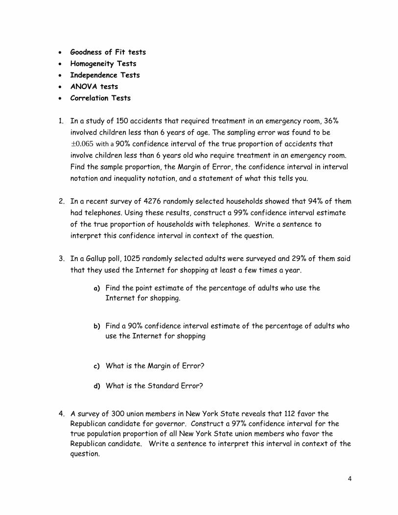
6. The following graph was made from the final exam scores of students in a Psychology
class. The mean average was 79 and the standard deviation was 5.7. Use the mean and
standard deviation to find the typical range (1 standard deviation) and the unusual range (2
standard deviations). Jimmy scored a 66% on the final. Was that unusual? Jake scored a
90% on the final. Was that unusual?
9590858075706560
35
30
25
20
15
10
5
0
C1
Fre
qu
en
cy
Histogram of C1
Confidence Intervals and Hypothesis Test Review
Topics:
Sampling Variability and Sampling Distributions
Confidence intervals for proportions (1 and 2 proportions)
Confidence intervals for means (1 mean, 2 independent means, matched pairs)
Analyzing confidence intervals, Finding sample values and margin of error
Using simulation to understand hypothesis testing
Hypothesis testing for proportions (1 and 2 proportion)
Hypothesis testing for means (1 mean, 2 independent means, matched pairs)
Analyzing type I and type II errors
4
Goodness of Fit tests
Homogeneity Tests
Independence Tests
ANOVA tests
Correlation Tests
1. In a study of 150 accidents that required treatment in an emergency room, 36%
involved children less than 6 years of age. The sampling error was found to be
0.065 with a 90% confidence interval of the true proportion of accidents that
involve children less than 6 years old who require treatment in an emergency room.
Find the sample proportion, the Margin of Error, the confidence interval in interval
notation and inequality notation, and a statement of what this tells you.
2. In a recent survey of 4276 randomly selected households showed that 94% of them
had telephones. Using these results, construct a 99% confidence interval estimate
of the true proportion of households with telephones. Write a sentence to
interpret this confidence interval in context of the question.
3. In a Gallup poll, 1025 randomly selected adults were surveyed and 29% of them said
that they used the Internet for shopping at least a few times a year.
a) Find the point estimate of the percentage of adults who use the
Internet for shopping.
b) Find a 90% confidence interval estimate of the percentage of adults who
use the Internet for shopping
c) What is the Margin of Error?
d) What is the Standard Error?
4. A survey of 300 union members in New York State reveals that 112 favor the
Republican candidate for governor. Construct a 97% confidence interval for the
true population proportion of all New York State union members who favor the
Republican candidate. Write a sentence to interpret this interval in context of the
question.
5
5. Test the claim that the proportion of drowning deaths of children attributable to
beaches is more than 25%. A sample of 615 drowning deaths showed that 30% of
them were attributable to beaches. Use α = 0.01.
6. The Harris Poll conducted a survey in which they asked “How many tattoos do you
currently have on your body?” Of the 1,205 males surveyed, 181 responded that
they had at least one tattoo. Of the 1,097 females surveyed, 143 responded that
they had at least one tattoo. At level of significance of 0.05, is the difference in
proportions of females that have at least one tattoo different from the proportion
of males that have at least one tattoo.
a) State the hypotheses
b) What kind of test do you have? (Right tailed-test, left tailed-test, or Two tailed-
test)
c) Find the critical value and the test statistic?
d) Find the P-value
e) Conclusion:
7. A study was conducted to assess the effects that occur when children are exposed
to cocaine before birth. Children were tested at age 4 for object assembly skills.
Of the 190 children born to cocaine users, 139 of them passed the test. Of the 186
children not exposed to cocaine, 153 of the children passed the test. Use 05.0
to test the claim that prenatal cocaine exposure is associated with lower scores of
four year-old children on the test of object assembly.
8. Identifying a type I error and the type II error that correspond to the given
hypothesis. A toy company is concerned with child safety. They want more than
98% of their pre-school toys to not have small parts that children can choke on.
a. Write a conclusion that would result from a type I error.
b. Write a conclusion that would result from a type II error.
6
9. Julie is curious about salaries at the company she works for. She wants to know if
managers make more than the regular employees and if so, how much more? A
random sample of 16 managers had an average salary of $65,000 with a standard
deviation of $12,000. A random sample of 45 regular employees had an average
salary of $46,000 with a standard deviation of $7,500. A histogram of the
managers showed a bell shaped distribution. Answer the following questions.
a) Does this problem meet the assumptions necessary to perform hypothesis tests
and confidence intervals for two means? Explain.
b) Are the two data sets independent or matched pairs? Explain.
c) Use Statcato and a 5% significance level to test the claim that managers make
more money than regular employees. Be sure to give the null and alternative
hypothesis, the test statistic, the p-value, whether you reject the null hypothesis
and a conclusion. Write a sentence explaining the test statistic and a sentence
explaining the p-value.
d) Create a two mean 90% confidence interval to estimate the difference
between the manager’s average salary and the regular employee’s average salary.
Write a sentence explaining the interval. What does 90% confident mean? Does
the interval agree with the hypothesis test?
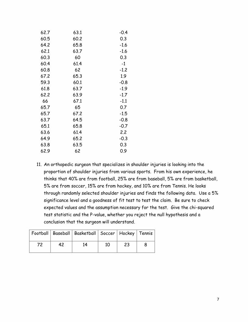
10. Are daughters always taller than their moms? This is the question we want to look
into. The following data set shows gives the height of 20 randomly selected moms
and the corresponding heights of their daughters.
a) Does this problem meet the assumptions necessary to perform hypothesis tests
and confidence intervals for two means?
b) Are the two data sets independent or matched pairs? Explain.
c) Use Statcato and a 10% significance level to test the claim that mothers are the
same height as their daughters. Be sure to give the null and alternative hypothesis,
the test statistic, the p-value, whether you reject the null hypothesis and a
conclusion. Write a sentence explaining the test statistic and a sentence explaining
the p-value.
d) Construct a 90% confidence interval for the difference between the mom’s
height and the daughter’s height. Write a sentence that interprets the interval.
Does the confidence interval agree with the hypothesis test in step (c)? Why?
Mom's
Height
Daughter's
Height
Difference (mom-
daughter)
7
62.7 63.1 -0.4
60.5 60.2 0.3
64.2 65.8 -1.6
62.1 63.7 -1.6
60.3 60 0.3
60.4 61.4 -1
60.8 62 -1.2
67.2 65.3 1.9
59.3 60.1 -0.8
61.8 63.7 -1.9
62.2 63.9 -1.7
66 67.1 -1.1
65.7 65 0.7
65.7 67.2 -1.5
63.7 64.5 -0.8
65.1 65.8 -0.7
63.6 61.4 2.2
64.9 65.2 -0.3
63.8 63.5 0.3
62.9 62 0.9
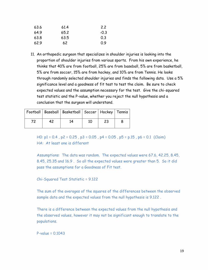
11. An orthopedic surgeon that specializes in shoulder injuries is looking into the
proportion of shoulder injuries from various sports. From his own experience, he
thinks that 40% are from football, 25% are from baseball, 5% are from basketball,
5% are from soccer, 15% are from hockey, and 10% are from Tennis. He looks
through randomly selected shoulder injuries and finds the following data. Use a 5%
significance level and a goodness of fit test to test the claim. Be sure to check
expected values and the assumption necessary for the test. Give the chi-squared
test statistic and the P-value, whether you reject the null hypothesis and a
conclusion that the surgeon will understand.
Football Baseball Basketball Soccer Hockey Tennis
72 42 14 10 23 8
8
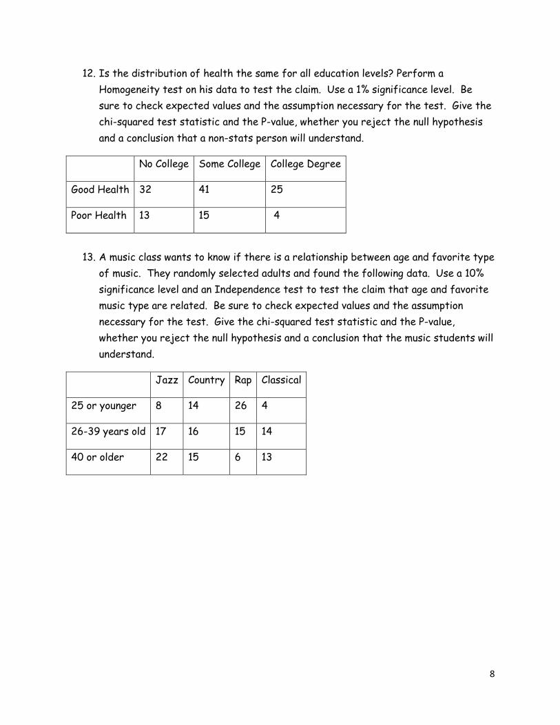
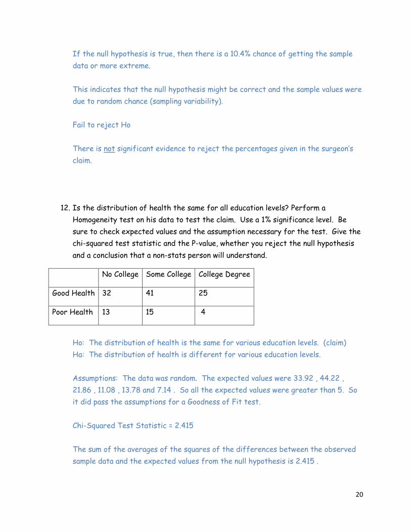
12. Is the distribution of health the same for all education levels? Perform a
Homogeneity test on his data to test the claim. Use a 1% significance level. Be
sure to check expected values and the assumption necessary for the test. Give the
chi-squared test statistic and the P-value, whether you reject the null hypothesis
and a conclusion that a non-stats person will understand.
No College Some College College Degree
Good Health 32 41 25
Poor Health 13 15 4
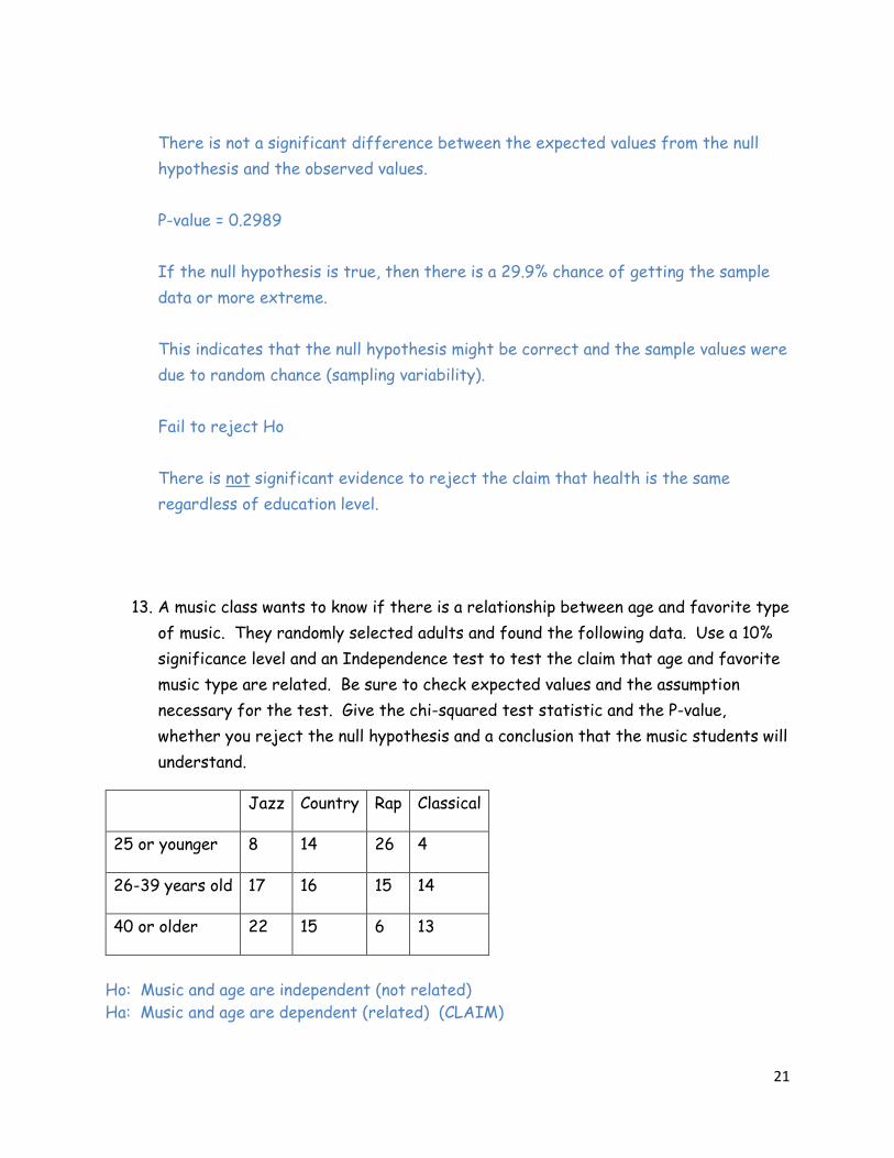
13. A music class wants to know if there is a relationship between age and favorite type
of music. They randomly selected adults and found the following data. Use a 10%
significance level and an Independence test to test the claim that age and favorite
music type are related. Be sure to check expected values and the assumption
necessary for the test. Give the chi-squared test statistic and the P-value,
whether you reject the null hypothesis and a conclusion that the music students will
understand.
Jazz Country Rap Classical
25 or younger 8 14 26 4
26-39 years old 17 16 15 14
40 or older 22 15 6 13
9
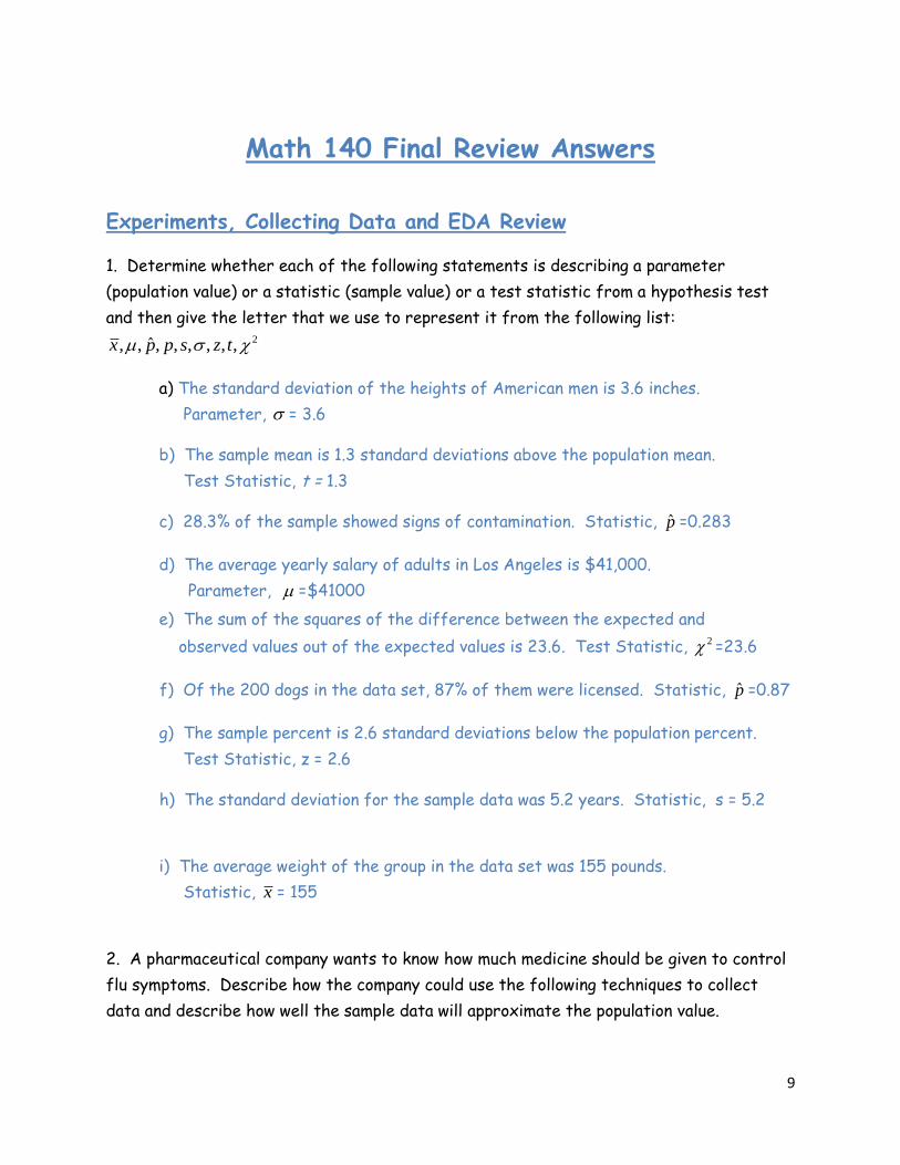
Math 140 Final Review Answers
Experiments, Collecting Data and EDA Review
1. Determine whether each of the following statements is describing a parameter
(population value) or a statistic (sample value) or a test statistic from a hypothesis test
and then give the letter that we use to represent it from the following list: 2ˆ, , , , , , , ,x p p s z t
a) The standard deviation of the heights of American men is 3.6 inches.
Parameter, = 3.6
b) The sample mean is 1.3 standard deviations above the population mean.
Test Statistic, t = 1.3
c) 28.3% of the sample showed signs of contamination. Statistic, p̂ =0.283
d) The average yearly salary of adults in Los Angeles is $41,000.
Parameter, =$41000
e) The sum of the squares of the difference between the expected and
observed values out of the expected values is 23.6. Test Statistic, 2 =23.6
f) Of the 200 dogs in the data set, 87% of them were licensed. Statistic, p̂ =0.87
g) The sample percent is 2.6 standard deviations below the population percent.
Test Statistic, z = 2.6
h) The standard deviation for the sample data was 5.2 years. Statistic, s = 5.2
i) The average weight of the group in the data set was 155 pounds.
Statistic, x = 155
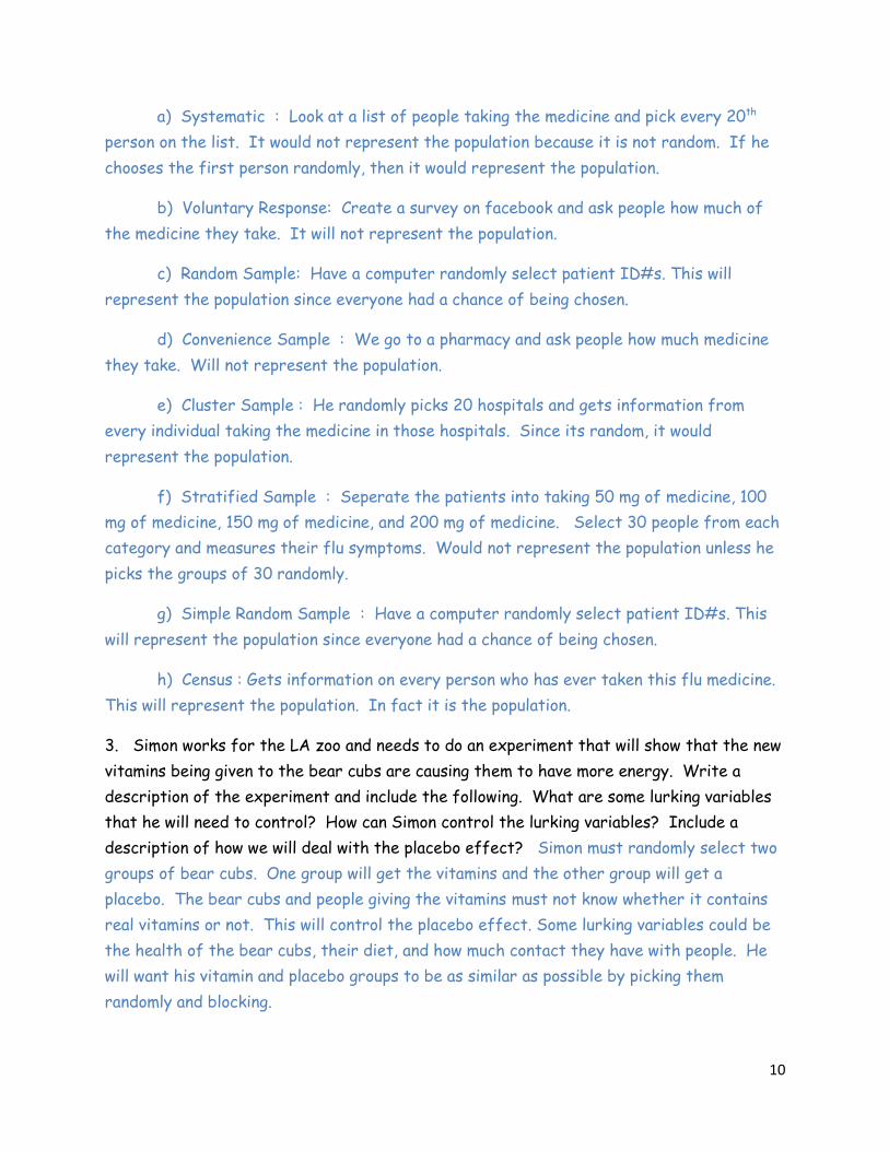
2. A pharmaceutical company wants to know how much medicine should be given to control
flu symptoms. Describe how the company could use the following techniques to collect
data and describe how well the sample data will approximate the population value.
10
a) Systematic : Look at a list of people taking the medicine and pick every 20th
person on the list. It would not represent the population because it is not random. If he
chooses the first person randomly, then it would represent the population.
b) Voluntary Response: Create a survey on facebook and ask people how much of
the medicine they take. It will not represent the population.
c) Random Sample: Have a computer randomly select patient ID#s. This will
represent the population since everyone had a chance of being chosen.
d) Convenience Sample : We go to a pharmacy and ask people how much medicine
they take. Will not represent the population.
e) Cluster Sample : He randomly picks 20 hospitals and gets information from
every individual taking the medicine in those hospitals. Since its random, it would
represent the population.
f) Stratified Sample : Seperate the patients into taking 50 mg of medicine, 100
mg of medicine, 150 mg of medicine, and 200 mg of medicine. Select 30 people from each
category and measures their flu symptoms. Would not represent the population unless he
picks the groups of 30 randomly.
g) Simple Random Sample : Have a computer randomly select patient ID#s. This
will represent the population since everyone had a chance of being chosen.
h) Census : Gets information on every person who has ever taken this flu medicine.
This will represent the population. In fact it is the population.
3. Simon works for the LA zoo and needs to do an experiment that will show that the new
vitamins being given to the bear cubs are causing them to have more energy. Write a
description of the experiment and include the following. What are some lurking variables
that he will need to control? How can Simon control the lurking variables? Include a
description of how we will deal with the placebo effect? Simon must randomly select two
groups of bear cubs. One group will get the vitamins and the other group will get a
placebo. The bear cubs and people giving the vitamins must not know whether it contains
real vitamins or not. This will control the placebo effect. Some lurking variables could be
the health of the bear cubs, their diet, and how much contact they have with people. He
will want his vitamin and placebo groups to be as similar as possible by picking them
randomly and blocking.
11
4. Tell if the following data is categorical or quantitative. If the data set is quantitative
and we created a histogram for the data, what do you think the shape would look like?
Why can’t we find the shape for categorical data?
a) The types of cars in the different COC parking Lots. Categorical
b) The average number of hours spent practicing ping pong.
Quantitative , Skewed Right
c) The number of wild mustang horses in various herds across the U.S.
Quantitative, Bell shaped
d) Each person is asked if they wear glasses, contacts, neither, or both.
Categorical
e) The average speed of the race cars at the Indianapolis 500.
Quantitative , Bell shaped
f) The test scores on a really difficult test. Quantitative , Skewed right
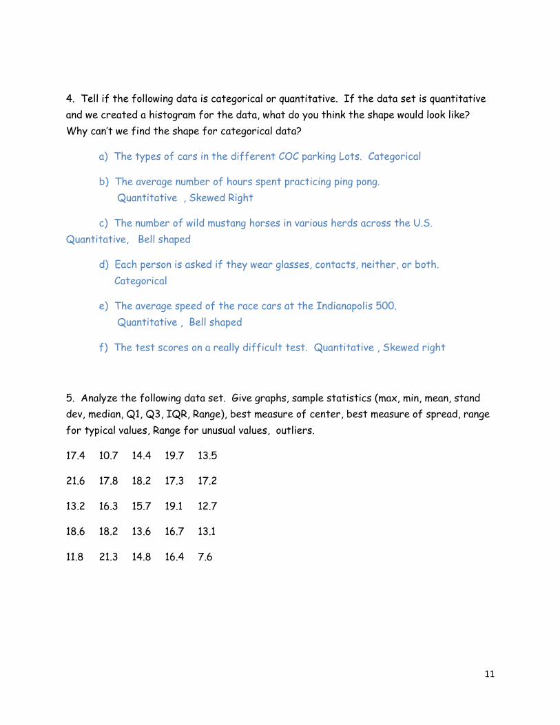
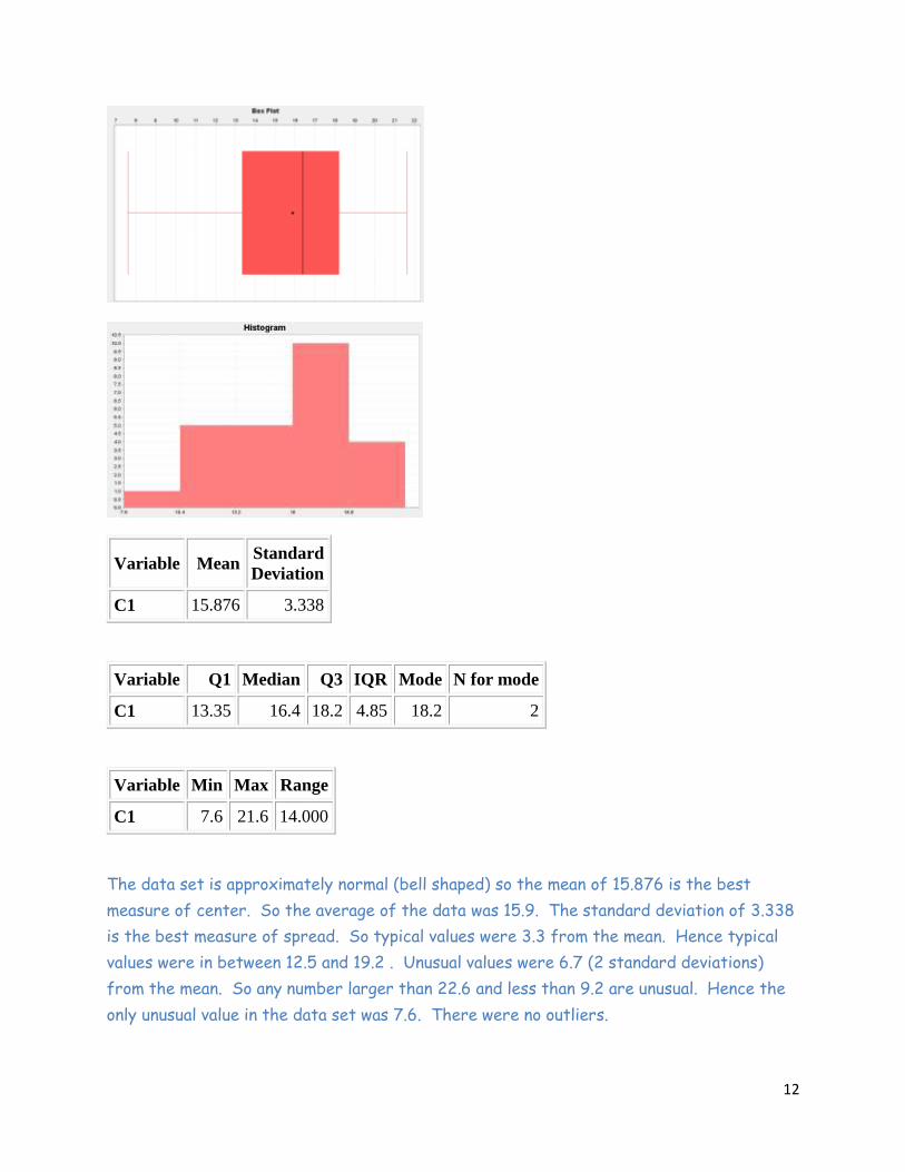
5. Analyze the following data set. Give graphs, sample statistics (max, min, mean, stand
dev, median, Q1, Q3, IQR, Range), best measure of center, best measure of spread, range
for typical values, Range for unusual values, outliers.
17.4 10.7 14.4 19.7 13.5
21.6 17.8 18.2 17.3 17.2
13.2 16.3 15.7 19.1 12.7
18.6 18.2 13.6 16.7 13.1
11.8 21.3 14.8 16.4 7.6
12
Variable Mean Standard
Deviation
C1 15.876 3.338
Variable Q1 Median Q3 IQR Mode N for mode
C1 13.35 16.4 18.2 4.85 18.2 2
Variable Min Max Range
C1 7.6 21.6 14.000
The data set is approximately normal (bell shaped) so the mean of 15.876 is the best
measure of center. So the average of the data was 15.9. The standard deviation of 3.338
is the best measure of spread. So typical values were 3.3 from the mean. Hence typical
values were in between 12.5 and 19.2 . Unusual values were 6.7 (2 standard deviations)
from the mean. So any number larger than 22.6 and less than 9.2 are unusual. Hence the
only unusual value in the data set was 7.6. There were no outliers.
13
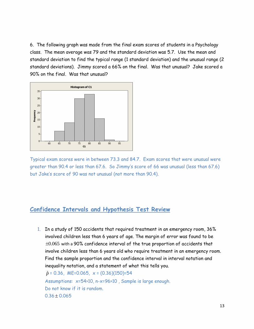
6. The following graph was made from the final exam scores of students in a Psychology
class. The mean average was 79 and the standard deviation was 5.7. Use the mean and
standard deviation to find the typical range (1 standard deviation) and the unusual range (2
standard deviations). Jimmy scored a 66% on the final. Was that unusual? Jake scored a
90% on the final. Was that unusual?
9590858075706560
35
30
25
20
15
10
5
0
C1
Fre
qu
en
cy
Histogram of C1
Typical exam scores were in between 73.3 and 84.7. Exam scores that were unusual were
greater than 90.4 or less than 67.6. So Jimmy’s score of 66 was unusual (less than 67.6)
but Jake’s score of 90 was not unusual (not more than 90.4).
Confidence Intervals and Hypothesis Test Review
1. In a study of 150 accidents that required treatment in an emergency room, 36%
involved children less than 6 years of age. The margin of error was found to be
0.065 with a 90% confidence interval of the true proportion of accidents that
involve children less than 6 years old who require treatment in an emergency room.
Find the sample proportion and the confidence interval in interval notation and
inequality notation, and a statement of what this tells you.
p̂ = 0.36, ME=0.065, x = (0.36)(150)=54
Assumptions: x=54>10, n-x=96>10 , Sample is large enough.
Do not know if it is random.
0.36 0.065
14
(0.295, 0.425)
0.295 < p < 0.425
We are 90% confident that the true proportion of accidents involving children less
than 6 years old is between 29.5% and 42.5%.
2. In a recent survey of 4276 randomly selected households showed that 94% of them
had telephones. Using these results, construct a 99% confidence interval estimate
of the true proportion of households with telephones. Write a sentence to
interpret this confidence interval in context of the question. What does 99%
confident mean?
p̂ = 0.94 , x = (0.94)(4276)=4019 >10 , n-x=257 >10 . The data set is large enough
and random so we can use it to make the confidence interval.
(0.931, 0.949)
We are 99% confident that the true population proportion of households with a
telephone is between 93.1% and 94.9%.
99% confident means that 99% of confidence intervals created contain the true
population proportion.
3. In a Gallup poll, 1025 randomly selected adults were surveyed and 29% of them said
that they used the Internet for shopping at least a few times a year.
e) Find the point estimate of the percentage of adults who use the
Internet for shopping. p̂ = 0.29 or 29%
f) Find a 90% confidence interval estimate of the percentage of adults who
use the Internet for shopping
X = 1025(.29)=297>10 , N-X = 1025-297=728>10 , Since the data is
random and large enough it meets the assumptions.
(0.267 , 0.313)
g) What is the Margin of Error? ME=0.023
h) What is the Standard Error? Standard error = ME/1.645 = 0.014
4. A survey of 300 union members in New York State reveals that 112 favor the
Republican candidate for governor. Construct a 97% confidence interval for the
true population proportion of all New York State union members who favor the
Republican candidate. Write a sentence to interpret this interval in context of the
15
question.
X=112>10 and N-X=188>10. The data set is large enough,
but not necessarily random.
(0.312 , 0.434)
We are 97% confident that the true population proportion of all New York State
union members who favor the republican candidate is between 31.2% and 43.4%.
5. Test the claim that the proportion of drowning deaths of children attributable to
beaches is more than 25%. A sample of 615 drowning deaths showed that 30% of
them were attributable to beaches. Use α = 0.01.
H0: p = 0.25
HA: p >0.25 (claim)
p̂ =0.3 , x = 0.3(615)=185>10 , n-x = 430>10. The data is large enough but
not necessarily random. So it does not meet all the assumptions.
Test Statistic Z = 2.864 , So the sample percent of 30% is 2.86 standard
deviations above the population percent of 25%. P-value = 0.0018 . If the true
percent of deaths at the beach is 25%, then there is a 0.0018 chance of getting
112 out of 300 deaths at the beach. The Pvalue is less than sig level of 0.01.
Reject H0. There is significant sample evidence to support the claim that the
proportion of drowning deaths of children attributed to beaches is more than 25%.
6. The Harris Poll conducted a survey in which they asked “How many tattoos do you
currently have on your body?” Of the 1,205 males surveyed, 181 responded that
they had at least one tattoo. Of the 1,097 females surveyed, 143 responded that
they had at least one tattoo. At level of significance of 0.05, is the difference in
proportions of females that have at least one tattoo different from the proportion
of males that have at least one tattoo.
f) State the hypotheses
H0: Pm = Pf or Pm-Pf=0
HA: Pm Pf or Pm-Pf 0
g) What kind of test do you have? (Right tailed-test, left tailed-test, or Two tailed-
test)
2 Tails
h) Find the critical value and the test statistic? Test Stat z = 1.372 , Crit Value =
1.96
16
i) Find the P-value P-value = 0.170 .
j) Conclusion: Since Pvalue > sig level, we fail to reject H0. Hence there is not
sufficient sample evidence to support the claim the proportion of males that have
at least one tattoo is different from the number of females with at least one
tattoo.
7. A study was conducted to assess the effects that occur when children are exposed
to cocaine before birth. Children were tested at age 4 for object assembly skills.
Of the 190 children born to cocaine users, 139 of them passed the test. Of the 186
children not exposed to cocaine, 153 of the children passed the test. Use 05.0
to test the claim that prenatal cocaine exposure is associated with lower scores of
four year-old children on the test of object assembly.
H0: Pc = Pn or Pc – Pn = 0
HA: Pc < Pn or Pc – Pn <0
Samples are large enough. (x >10 and N-x>10) , but not random samples so it does
not meet the assumptions.
Test Statistic z = -2.134
P-value = 0.0164. Since Pvalue < sig level 0.05 we reject H0. There is sufficient
evidence to support the claim that babies exposed to cocaine scored lower on the
object assembly test.
8. Identifying a type I error and the type II error that correspond to the given
hypothesis. A toy company is concerned with child safety. They want more than
98% of their pre-school toys to not have small parts that children can choke on.
H0: p = 0.98
HA: p > 0.98 (claim)
a. Write a conclusion that would result from a type I error.
A type I error means that we reject H0 and support claim by mistake. This
would result in the company thinking that their toys are safe when they are
really not. If children are hurt because of choking, the company may be
liable.
b. Write a conclusion that would result from a type II error.
A type I error means that we fail to reject H0 and do not support claim by
mistake. This would result in the company thinking that their toys are not
safe when they really are. The toy company may lose money by taking toys
off the market or doing more tests to make sure they are safe.
9. Julie is curious about salaries at the company she works for. She wants to know if
managers make more than the regular employees and if so, how much more? A
17
random sample of 16 managers had an average salary of $65,000 with a standard
deviation of $12,000. A random sample of 45 regular employees had an average
salary of $46,000 with a standard deviation of $7,500. A histogram of the
managers showed a bell shaped distribution. Answer the following questions.
a) Does this problem meet the assumptions necessary to perform hypothesis tests
and confidence intervals for two means? Explain. The data does meet the
assumptions necessary to proceed. The data is random and the regular employees >
30. The manager data set is too small but since it is normal we can proceed.
b) Are the two data sets independent or matched pairs? Explain. Independent
since there is no relationship between managers and regular employees.
c) Use Statcato and a 5% significance level to test the claim that managers make
more money than regular employees. Be sure to give the null and alternative
hypothesis, the test statistic, the p-value, whether you reject the null hypothesis
and a conclusion. Write a sentence explaining the test statistic and a sentence
explaining the p-value.
H0: mu1 = mu2 or mu1-mu2 = 0
HA: mu 1 > mu2 or mu1 – mu2 > 0
Test Stat T = 5.935 . So the difference between the sample salaries is 5.9
standard deviations above zero. P-value = 0.0000051596 . If the manager and
employee salaries are the same there was a 0.00000516 chance of getting the
sample data. Reject H0. There is significant sample evidence to support the claim
that managers make more than regular employees.
d) Create a two mean 90% confidence interval to estimate the difference
between the manager’s average salary and the regular employee’s average salary.
Write a sentence explaining the interval. What does 90% confident mean? Does
the interval agree with the hypothesis test?
(13464 , 24536) . We are 90% confident that managers make beteen $13464 and
$24536 more than regular employees. 90% of confidence intervals created will
contain the true difference between managers and regular employees.
10. Are daughters always the same height as their moms? This is the question we want
to look into. The following data set shows gives the height of 20 randomly selected
moms and the corresponding heights of their daughters.
a) Does this problem meet the assumptions necessary to perform hypothesis tests
and confidence intervals for two means? The data did not meet the assumptions
since the histograms were right skewed and too small (less than 30).
18
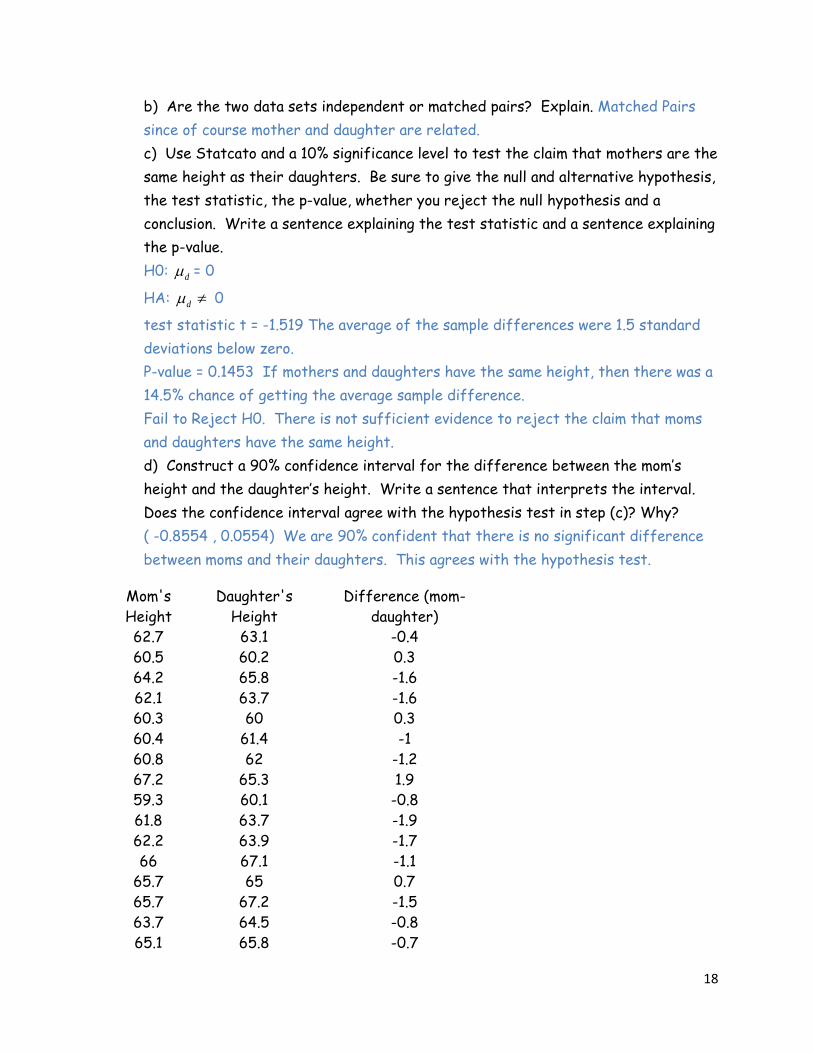
b) Are the two data sets independent or matched pairs? Explain. Matched Pairs
since of course mother and daughter are related.
c) Use Statcato and a 10% significance level to test the claim that mothers are the
same height as their daughters. Be sure to give the null and alternative hypothesis,
the test statistic, the p-value, whether you reject the null hypothesis and a
conclusion. Write a sentence explaining the test statistic and a sentence explaining
the p-value.
H0: d = 0
HA: d 0
test statistic t = -1.519 The average of the sample differences were 1.5 standard
deviations below zero.
P-value = 0.1453 If mothers and daughters have the same height, then there was a
14.5% chance of getting the average sample difference.
Fail to Reject H0. There is not sufficient evidence to reject the claim that moms
and daughters have the same height.
d) Construct a 90% confidence interval for the difference between the mom’s
height and the daughter’s height. Write a sentence that interprets the interval.
Does the confidence interval agree with the hypothesis test in step (c)? Why?
( -0.8554 , 0.0554) We are 90% confident that there is no significant difference
between moms and their daughters. This agrees with the hypothesis test.
Mom's
Height
Daughter's
Height
Difference (mom-
daughter)
62.7 63.1 -0.4
60.5 60.2 0.3
64.2 65.8 -1.6
62.1 63.7 -1.6
60.3 60 0.3
60.4 61.4 -1
60.8 62 -1.2
67.2 65.3 1.9
59.3 60.1 -0.8
61.8 63.7 -1.9
62.2 63.9 -1.7
66 67.1 -1.1
65.7 65 0.7
65.7 67.2 -1.5
63.7 64.5 -0.8
65.1 65.8 -0.7
19
63.6 61.4 2.2
64.9 65.2 -0.3
63.8 63.5 0.3
62.9 62 0.9
11. An orthopedic surgeon that specializes in shoulder injuries is looking into the
proportion of shoulder injuries from various sports. From his own experience, he
thinks that 40% are from football, 25% are from baseball, 5% are from basketball,
5% are from soccer, 15% are from hockey, and 10% are from Tennis. He looks
through randomly selected shoulder injuries and finds the following data. Use a 5%
significance level and a goodness of fit test to test the claim. Be sure to check
expected values and the assumption necessary for the test. Give the chi-squared
test statistic and the P-value, whether you reject the null hypothesis and a
conclusion that the surgeon will understand.
Football Baseball Basketball Soccer Hockey Tennis
72 42 14 10 23 8
H0: p1 = 0.4 , p2 = 0.25 , p3 = 0.05 , p4 = 0.05 , p5 = p.15 , p6 = 0.1 (Claim)
HA: At least one is different
Assumptions: The data was random. The expected values were 67.6, 42.25, 8.45,
8.45, 25.35 and 16.9 . So all the expected values were greater than 5. So it did
pass the assumptions for a Goodness of Fit test.
Chi-Squared Test Statistic = 9.122
The sum of the averages of the squares of the differences between the observed
sample data and the expected values from the null hypothesis is 9.122 .
There is a difference between the expected values from the null hypothesis and
the observed values, however it may not be significant enough to translate to the
populations.
P-value = 0.1043
20
If the null hypothesis is true, then there is a 10.4% chance of getting the sample
data or more extreme.
This indicates that the null hypothesis might be correct and the sample values were
due to random chance (sampling variability).
Fail to reject Ho
There is not significant evidence to reject the percentages given in the surgeon’s
claim.
12. Is the distribution of health the same for all education levels? Perform a
Homogeneity test on his data to test the claim. Use a 1% significance level. Be
sure to check expected values and the assumption necessary for the test. Give the
chi-squared test statistic and the P-value, whether you reject the null hypothesis
and a conclusion that a non-stats person will understand.
No College Some College College Degree
Good Health 32 41 25
Poor Health 13 15 4
Ho: The distribution of health is the same for various education levels. (claim)
Ha: The distribution of health is different for various education levels.
Assumptions: The data was random. The expected values were 33.92 , 44.22 ,
21.86 , 11.08 , 13.78 and 7.14 . So all the expected values were greater than 5. So
it did pass the assumptions for a Goodness of Fit test.
Chi-Squared Test Statistic = 2.415
The sum of the averages of the squares of the differences between the observed
sample data and the expected values from the null hypothesis is 2.415 .
21
There is not a significant difference between the expected values from the null
hypothesis and the observed values.
P-value = 0.2989
If the null hypothesis is true, then there is a 29.9% chance of getting the sample
data or more extreme.
This indicates that the null hypothesis might be correct and the sample values were
due to random chance (sampling variability).
Fail to reject Ho
There is not significant evidence to reject the claim that health is the same
regardless of education level.
13. A music class wants to know if there is a relationship between age and favorite type
of music. They randomly selected adults and found the following data. Use a 10%
significance level and an Independence test to test the claim that age and favorite
music type are related. Be sure to check expected values and the assumption
necessary for the test. Give the chi-squared test statistic and the P-value,
whether you reject the null hypothesis and a conclusion that the music students will
understand.
Jazz Country Rap Classical
25 or younger 8 14 26 4
26-39 years old 17 16 15 14
40 or older 22 15 6 13
Ho: Music and age are independent (not related)
Ha: Music and age are dependent (related) (CLAIM)

22
Assumptions: Expected values are 14.38 , 13.76 , 14.38 , 9.48 , 17.14 , 16.41 , 17.14 , 11.31 ,
15.48 , 14.82 , 15.48 and 10.21 . All expected values are at least 5. Since the data is also
random it meets the assumptions for a chi-squared independence test.
Chi-squared test statistic = 25.635 The sum of the averages of the squares of the
difference between the observed sample data and the expected values is 25.635 . This
indicates there is a significant difference between the observed sample data and the
expected values from the null hypothesis.
P-value = 0.0003 If the null hypothesis is true and age and music are independent, then
there was only a 0.0003 chance of getting this sample data or more extreme. It is
extremely unlikely that the null hypothesis was correct and this sample data just happened
by random chance (sampling variability).
Reject Ho
There is significant sample evidence to support the claim that age and music preferences
are related.