MATERIA¸Y I STUDIA - ssl.nbp.pl

Warsaw, September 2005

Fundamental equilibrium exchange

rate for the Polish zloty

MATERIA¸Y I STUDIA

Micha∏ Rubaszek

Paper No. 35

Micha∏ Rubaszek – Economist, Macroeconomic and Structural Analysis Department, National Bankof Poland and Econometrics Institute, Warsaw School of Economics.

E-mail: [email protected]

The opinions expressed in this paper are those of the author and should not be treated as theofficial position of the National Bank of Poland.

Author would like to thank Ryszard Kokoszczyƒski, Rebecca Driver, Jakub Borowski, Marek A.Dàbrowski and NBP economists for many useful comments that helped to improve the previousversions of this paper.

Design:

Oliwka s.c.

Layout and print:

NBP Printshop

Published by:

National Bank of PolandDepartment of Information and Public Relations00-919 Warszawa, 11/21 Âwi´tokrzyska Streetphone: (22) 653 23 35, fax (22) 653 13 21

© Copyright by the National Bank of Poland, 2005

http://www.nbp.pl

Contents

MATERIA¸Y I STUDIA PAPER 35 3

Contents

Tables and figures . . . . . . . . . . . . . . . . . . . . . . . . . . . . . . . . . . . . . . . . . . . . . . . . . . . . . . . 4

Abstract . . . . . . . . . . . . . . . . . . . . . . . . . . . . . . . . . . . . . . . . . . . . . . . . . . . . . . . . . . . . . . . . 5

Introduction . . . . . . . . . . . . . . . . . . . . . . . . . . . . . . . . . . . . . . . . . . . . . . . . . . . . . . . . . . . . 6

1. The model of fundamental equilibrium exchange rate . . . . . . . . . . . . . . . . . . . 7

2. Three inputs of the fundamental equilibrium exchange rate model . . . . . . 122.1. Foreign trade model . . . . . . . . . . . . . . . . . . . . . . . . . . . . . . . . . . . . . . . . . . . . . . . . . . . . 12

2.1.1. Export and import volumes of goods and services . . . . . . . . . . . . . . . . . . . . . . . . . . . 12

2.1.2. Export and import prices of goods and services . . . . . . . . . . . . . . . . . . . . . . . . . . . . 14

2.1.3. Simulations . . . . . . . . . . . . . . . . . . . . . . . . . . . . . . . . . . . . . . . . . . . . . . . . . . . . . . 15

2.2. Internal equilibrium . . . . . . . . . . . . . . . . . . . . . . . . . . . . . . . . . . . . . . . . . . . . . . . . . . . . . 15

2.3. External equilibrium . . . . . . . . . . . . . . . . . . . . . . . . . . . . . . . . . . . . . . . . . . . . . . . . . . . . . 16

3. The results . . . . . . . . . . . . . . . . . . . . . . . . . . . . . . . . . . . . . . . . . . . . . . . . . . . . . . . . . . 193.1. The level of the zloty’s fundamental equilibrium exchange rate . . . . . . . . . . . . . . . . . . . . . . 19

3.2. Sensitivity analysis . . . . . . . . . . . . . . . . . . . . . . . . . . . . . . . . . . . . . . . . . . . . . . . . . . . . . . 20

3.2.1. Foreign output gap . . . . . . . . . . . . . . . . . . . . . . . . . . . . . . . . . . . . . . . . . . . . . . . . 21

3.2.2. Domestic output gap . . . . . . . . . . . . . . . . . . . . . . . . . . . . . . . . . . . . . . . . . . . . . . . 21

3.2.3. Target level of balance on trade and services . . . . . . . . . . . . . . . . . . . . . . . . . . . . . . 22

4. Summary . . . . . . . . . . . . . . . . . . . . . . . . . . . . . . . . . . . . . . . . . . . . . . . . . . . . . . . . . . . 24

5. References . . . . . . . . . . . . . . . . . . . . . . . . . . . . . . . . . . . . . . . . . . . . . . . . . . . . . . . . . . 25

4

Tables and figures

N a t i o n a l B a n k o f P o l a n d

Tables and figures

Table 1 Countries’ share in the Polish foreign trade (%) . . . . . . . . . . . . . . . . . . . . . . . . . . . . . 13

Table 2 Cointegration trace test . . . . . . . . . . . . . . . . . . . . . . . . . . . . . . . . . . . . . . . . . . . . . . 14

Table 3 An impact of 10% permanent depreciation of the RER on foreign trade . . . . . . . . . . . 15

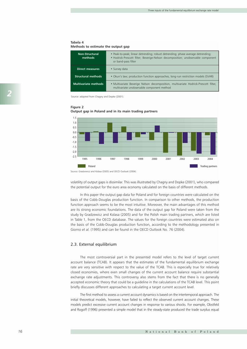
Table 4 Methods to estimate the output gap . . . . . . . . . . . . . . . . . . . . . . . . . . . . . . . . . . . . 16

Table 5 Balance on goods and services and output gap in Poland in 2004 . . . . . . . . . . . . . . . 20

Figure 1 Domestic demand and real exchange rate . . . . . . . . . . . . . . . . . . . . . . . . . . . . . . . . 11

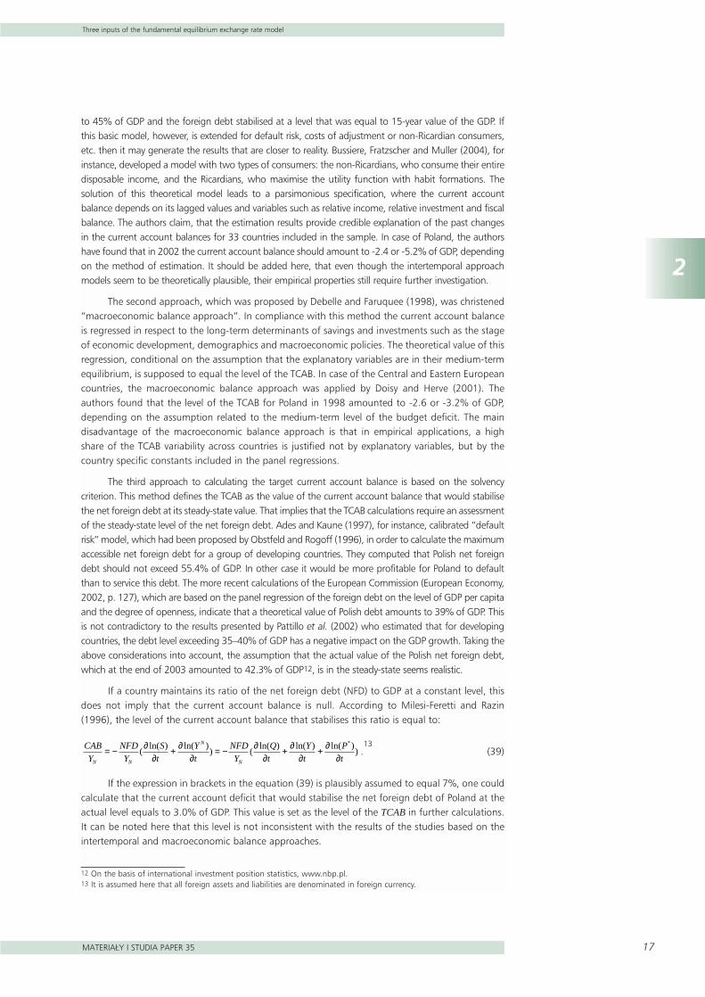
Figure 2 Output gap in Poland and in its main trading partners . . . . . . . . . . . . . . . . . . . . . . 16

Figure 3 Sensitivity of the zloty’s misalignment with respect to the assumed level of theforeign output gap . . . . . . . . . . . . . . . . . . . . . . . . . . . . . . . . . . . . . . . . . . . . . . . . 21

Figure 4 Sensitivity of the zloty’s misalignment with respect to the assumed level of thedomestic output gap . . . . . . . . . . . . . . . . . . . . . . . . . . . . . . . . . . . . . . . . . . . . . . . 22

Figure 5 The domestic demand and the real exchange rate in response to an increase inassumed level of domestic output gap . . . . . . . . . . . . . . . . . . . . . . . . . . . . . . . . . . 22

Figure 6 Sensitivity of the zloty’s misalignment with respect to the assumed value of thebalance on transfers . . . . . . . . . . . . . . . . . . . . . . . . . . . . . . . . . . . . . . . . . . . . . . . 23

Figure 7 The domestic demand and the real exchange rate in response an increase in thetarget level of the balance on goods and services . . . . . . . . . . . . . . . . . . . . . . . . . . 23

Abstract

MATERIA¸Y I STUDIA – PAPER 35 5

Abstract

In May 2004 Poland joined the European Union and is thereby committed to introduce the euroin the forthcoming years. The balance of costs and benefits of the euro adoption depends on thedecision of the Polish and European authorities concerning the level of central parity in the ERM II, andsubsequently the conversion rate of the zloty. In order to address the issue of an "ideal" level of the realexchange rate this paper proposes a model which is applied to estimate the level of the equilibrium ofthe zloty. The results indicate that at the end of 2004 the zloty was undervalued by 4.3%.

JEL classification: F12, F31, F41

Key words: conversion rate, equilibrium exchange rate, foreign trade model, cointegration

6

1

Introduction


Introduction

The studies of the development tendencies in the Polish economy in the late 1990s and atthe beginning of this millennium cannot neglect the influence of the foreign sector on theeconomic situation of the country. In this period Polish current and capital accounts were fullyliberalised. The Polish economy became more open: the volume of imports and exports multipliedfive and threefold, respectively (Mroczek, Rubaszek, 2003 and 2004). As a consequence, the impactof exchange rate fluctuations on Polish economy increased considerably.

In May 2004 Poland joined the European Union and thus became obliged to introduce theeuro in the forthcoming years. Among the benefits of joining the Monetary Union, which arediscussed in Borowski (2004), one can number lower costs of borrowing, elimination of theexchange rate risk, better access to foreign capital and lower transaction costs. These advantagesof the single currency seem to outweigh its major cost, i.e. loss of monetary policy independence.The balance of costs and benefits of euro adoption also depends on the decision of the Polish andEuropean authorities concerning the level of the central parity in the ERM II, and subsequently theconversion rate of the zloty. More precisely, inappropriate determination of the conversion rate mayinvoke severe consequences for the real sector of Polish economy. On the one hand, an overvaluedrate leads to a loss of competitiveness of domestic producers and hence forces them to limit theiroutput or even may drive them bankrupt. If prices are sticky and the adjustment slow, an overvaluedconversion rate may dampen domestic output for a prolonged period of time. On the other hand,an undervalued rate results in ineffective allocation of capital as the companies that are notcompetitive can expand their activity. Moreover, the purchasing parity of domestic wages issubdued, which might not optimise consumers’ welfare. Finally, weak currency brings aboutinflationary pressure, which in an environment of externally set nominal interest rates may lead toan unsustainable consumption boom. The above considerations lead us to the conclusion that theconversion rate should equal the equilibrium exchange rate of the zloty to maximise the net gainof adopting the euro.

In the case of the central parity in the ERM II the problem is more complicated. It may occurthat setting the entry rate at the equilibrium level may be suboptimal. An overvalued parity couldbe a better choice in the situation of excessive inflation, for instance. An undervalued parity wouldbe recommended if domestic demand was subdued. It should be emphasised, however, thatmisaligned ERM II parity may entail speculative attacks that would lead to severe problems withmaintaining the zloty within the fluctuation bands.

In order to address the issue of an “ideal” level of the real exchange rate this paperdescribes one of the most popular methods of the equilibrium exchange rate calculation, namelythe model of fundamental equilibrium exchange rate (FEER, Williamson 1983). A modification ofthis model is used to estimate the equilibrium level of the zloty in the forth quarter of 2004. Itwas found that in this period the quarterly average value of the real effective rate of the zlotywas 4.3% weaker than its fundamental value. This result, however, is subject to uncertainty as itdepends on a set of assumptions. In order to address this issue a thorough sensitivity analysiswas performed. Among others, the impact of EU transfers on the level of the equilibriumexchange rate was investigated.

The paper is organised as follows. The first section provides a description of the FEER model.The second part focuses on three issues related to the fundamental equilibrium exchange rate. Theestimation of the foreign trade model and the assessment of the level of the internal and externaldisequilibria can be found there. The third section presents the results of the calculations and thesensitivity analysis. The paper concludes with a summary of the obtained results and the descriptionof related issues.

2

The model of fundamental equilibrium exchange rate


1 The model of fundamental equilibrium exchange rate

The fundamental equilibrium exchange rate model is probably the most popular method ofcalculating the equilibrium exchange rate (MacDonald 2000). On the basis of this model, which is alsoreferred to as the internal-external balance model, it is possible to compute the level of the real exchangerate that is consistent with simultaneous attainment of the internal and external equilibria. In this paper,the internal equilibrium means that the actual output is equal to its potential level, i.e. the output gap isnull. The external equilibrium is defined as attainment of some target level of the current account balancethat corresponds to optimal portfolio allocation. In this sense, the fundamental equilibrium exchange ratemay be characterised as the level of the exchange rate that is consistent with ideal macroeconomicperformance (Williamson 1994, p. 180). It should be pointed out that in the short-term horizon the FEERmight not be the optimal level of the exchange rate if the economy is not in the equilibrium. Take atemporary undervalued exchange rate for instance: it would be recommended in case of a weak domesticoutput. By contrast, a temporary overvaluation would be helpful to contain inflationary pressure.

According to MacDonald (2000) there are two methods of estimating the fundamentalequilibrium exchange rate. The first one is based on a full-scale macroeconomic model. The FEER is thelevel of the exchange rate that would remain if all markets were in equilibrium. The advantage of thisapproach is that most of the model’s variables are endogenous and thus the calculated exchange rateis consistent with a well defined economic equilibrium. Moreover, on the basis of such model one cancalculate the short-term dynamics towards the long-term steady-state. The disadvantage of thisapproach is that it requires a sophisticated macroeconomic model, which has a well-defined steady-state solution. In practice, the construction of such a model tends to be very difficult and time-consuming. Moreover, the final results might be non-transparent, especially if the model is verycomplex. The alternative and less sophisticated partial equilibrium approach limits the group ofendogenous variables to a few variables related to foreign sector of the economy. It means thatdomestic prices, domestic demand, employment, money supply and other quantities are treated asexogenous. In this approach, one focuses solely on the external equilibrium condition, with theexchange rate functioning as a control variable. More precisely, partial-approach FEER is the level ofexchange rate that makes the current account balance equal to its target level, given that other marketsare in equilibrium. The main shortcoming of the partial equilibrium model is that it does not explain thebehaviour of the whole economy and does not provide any information about the short-term dynamics.Its major advantages over the full-equilibrium approach are simplicity and transparency.

The present paper develops an extended version of the partial fundamental equilibriumexchange rate model presented by Bayoumi and Faruqee (1998). The authors proposed a system withone control variable (real exchange rate) and one target variable (current account balance). In thispaper the specification with two control variables (real exchange rate and domestic demand) and twotarget variables (gross domestic product and current account balance) is proposed. Our modificationwas intended to make the model better suited to the Polish realities, especially as an inflow of EUtransfers is concerned. In the BF model, a positive EU transfer shock has an impact on externalequilibrium (higher current account balance) but do not affect internal equilibrium, as output gap isexogenous. To restore the external equilibrium, solely real exchange rate appreciation is required. Inthis sense, an inflow of EU funds in the BF model has the effects that are characteristic for Dutchdisease. In our model, an adjustment to a positive EU transfer shock differs from that in the BF model.In order to restore equilibrium an increase in domestic demand and real exchange rate appreciationis required. This seems more realistic, as an inflow of foreign transfers stimulates domestic demandand imports. This, in turn, deteriorates current account balance. As a result, required real exchangerate adjustments are of lower extent than in the BF model.

8

1



It should be emphasised, that in equilibrium, the level of domestic demand may depend onthe level of real exchange rate. Let us take the terms-of-trade effect for instance: real exchange rateappreciation leads to an improvement of the terms-of-trade and consequently in order to financea given amount of imports a country can export less. This allows for domestic demand expansion.This effect for Germany was found by Meier (2004). As our model can be classified as partialequilibrium, in order to keep its small size and transparency we assume that domestic demand andreal exchange rate are independent. A detailed description of the model is presented below.

Goods markets at home and abroad are in equilibrium, when the actual output (Y) is equalto its potential level ( ). Therefore, the internal equilibrium condition is met when:

(1)

, (2)

where “*” stands for foreign variables.

The real sector in our model is described by two identities and two behavioural equations. Inequations (3) and (4) the domestic output (Y) is defined as the sum of domestic demand (DD) andnet exports (NT), where net exports is the difference between exports (X) and imports (M):

(3)

. (4)

It is supposed that in the long run the level of domestic exports (XS) is determined by supplyfactors, as Poland is a small open economy. If companies produce subject to the transformationfunction with constant transformation elasticity (α1) then the first-order condition of profitsmaximisation leads to the following relationship between exports, domestic output and relative prices1:

, α0>0 α1>0 (5)

where PX and P stand for export and domestic prices, respectively. In the short run, thedeviation of the actual exports from its supply level given by (5) depends on demand factors, suchas the foreign demand and price competitiveness of domestic exports on the foreign market:

, f1>0, f2<0 (6)

where P* /S is the level of foreign prices expressed in units of domestic currency.

Subsequently, the level of domestic imports is entirely determined by demand factors as it issupposed that the foreign supply is infinite. As imported and domestically produced goods are assumedto be imperfect substitutes and the utility function is in CES form, the first-order condition of the utilitymaximisation leads to the following relationship between imports, total demand and relative prices:

, β0>0, β1>0 (7)

where PM stands for import prices.

The external equilibrium in the model is defined as attainment of some target level of thecurrent account balance:

, (8)

where CAB and TCAB are actual and target levels of the current account balance, respectively. Onecan notice that as the internal and external equilibria are expressed in flow terms, the fundamentalequilibrium exchange rate is a medium-term concept.

CAB TCAB=

MP tariff

PYM= +

−

ββ

0

1 1( )

X

Xf

Y

Y

P tariff

P SSX= +

( ,( )

/)

*

* *

1

XP

PYS X=

α

α

0

1

NT X M= −

Y DD NT= +

Y Y* *=

Y Y=

Y

1 We assume that exports subsidies are negligible.

2



The nominal sector in the model is described by three identities and two behavioural equations.The current account balance is the sum of three components: the trade balance (CAB_TB)2, thebalance on income (CAB_INC) and the balance on transfers (CAB_TRANS).

. (9)

The trade balance is the difference between the nominal exports and the nominal imports:

. (10)

The third identity relates the nominal output to the product of the real output and domestic prices:

. (11)

The two behavioural equations are related to export and import prices. Assuming that the“price taker – price maker” hypothesis holds, these indices can be expressed as a weighted averageof domestic and foreign prices:

, γ0>0, γ1∈ <0,1> (12)

. δ0>0, δ1∈ <0,1> (13)

For countries that are price makers the elasticities γ1 and δ1 are close to unity. By contrast, theprice taker economies are characterised by values of these parameters close to zero.

Finally, let us define the real exchange rate (Q) as a relative price of domestic goods to foreign goods:

,(14)

where an increase in S and Q stands for appreciation in the domestic currency.

On the basis of the above system, which is described by equations (1)–(14), one can estimatethe levels of the domestic demand (DD) and the real exchange rate (Q) that would ensure theoccurrence of the internal and external equilibria. These “ideal” values of the domestic demand andthe real exchange rate, which will be referred to as DDFEER and QFEER, depend on the assumedvalues of the exogenous variables, namely the target level of the current account, the balance ontransfers, potential outputs and others.

The solution of the above system is as follows. On the basis of the equations (12), (13) and(14) one can calculate that the relative prices that have an impact on the export and import volumesaccording to (5), (6) and (7) depend solely on the level of the real exchange rate:

(15)

(16)

(17)

Equation (15) states that the appreciation of the real exchange rate leads to a fall in theprofitability of exports. In effect, the level of exports is declining in line with the relationship (5). Theprice competitiveness of home-produced goods on foreign markets is also deteriorating in responseto the strengthening of the domestic currency, which is shown in (16). Consequently, the demandfor exports is falling in line with the relationship (6). Finally, according to the equation (17), the pricecompetitiveness of the imported goods is rising in response to a real exchange rate appreciation.As a result, the volume of imports is increasing (see eq. 7).

P

P

P P S

PQ

M

= =−

−δ δδ δ

δ01

01

1 1

1( / )* ( )

( )

P

P S

P P S

P SQ

X

*

* ( )

*/( / )

/= =

−γ γγ γ

γ01

0

1 1

1

P

P

P P S

PQ

X

= =−

−γ γγ γ

γ01

01

1 1

1( / )* ( )

( )

QP

P S= * /

P P P SM = −δ δ δ0

11 1( / )* ( )

P P P SX = −γ γ γ0

11 1( / )* ( )

Y PYN =

CAB TB P X P MX M_ = −

CAB CAB TB CAB INC CAB TRANS= + +_ _ _

2 Trade balance equals balance on goods and services.

10

1



It can be concluded that the appreciation entails a decrease in exports and an increase inimport volumes and thus it deteriorates net exports. Furthermore, if in the identity (4) X and M aresubstituted by the expressions (5) and (7), and the relationships (1), (14) and (16) are taken intoaccount, one can calculate that in the long-run net exports (NTLR) equal to3:

. (18)

This expression can be transformed so that in the long run the ratio of net exports to outputdepends solely on the level of the real exchange rate:

, (19)

where the first derivative:

. (20)

In the short-term horizon, apart from the real exchange rate, net exports are also determinedby other factors, namely domestic and foreign demand (see equations 3–7):

. g1<0, g2∈ (-1, 0), g3>0 (21)

The partial derivative with respect to domestic demand is greater than -1 to ensure that thegrowth of domestic demand has a positive impact on the total output, i.e. .

Let us now focus on the trade balance, which is described by the identity (10). If the valuesof X, M, PX and PM are taken from the expressions (5), (7), (14) and (16), respectively, and thecondition (1) holds, one can express the long-term value of this balance as:

. (22)

This expression can be transformed so that in the long run the ratio of the trade balance tothe nominal output depends solely on the level of the real exchange rate:

. (23)

The sign of the first derivative:

(24)

may be ambiguous. We assume that the values of the relevant parameters ensure that thisexpression is negative and hence the Marshall-Lerner condition holds.

In the short-term horizon, apart from the real exchange rate, the trade balance is alsodetermined by other factors like the demand at home and abroad:

, h1<0, h2<0, h3>0. (25)

In accordance with the equations (1), (3) and (21) the levels of the real exchange rate (Q) anddomestic demand (DD) that would ensure the occurrence of the internal equilibrium can be calculated.In equilibrium, in order to guarantee that the actual output equals its potential level, a rise in domesticdemand requires a fall in net exports of the same value. This implies that domestic currency mustappreciate. As a result, the real exchange rate is an increasing function of the domestic demand:

, where (26)∂∂

>Q

DD0Q ie DD= ( ,...

CAB TB h Q DD Y_ ( , , ,...)*=

d CAB TB Y

dQQ Q

LRN( _ / )

( )( ) ( )( )( ) ( )( ) ( ) ( )( )= + − − − −+ + − − − − − −α α γ γ β β δ δα α γ β β δ0 1 1 0

1 1 1 10 1 1 0

1 1 1 11 1 1 11 1 1 1 1 1

CAB TB Y Q QLRN_ / = ( ) − ( )− + − −

α γ β δγ α δ β

0 01 1

0 01 1

1 1 11

CAB TB Q PY Q PYLR_ = ( ) − ( )− + − −α γ β δγ α δ β

0 01 1

0 01 1

1 1 11

dY

dDD> 0

NT g Q DD Y= ( , , ,...)*

d NT Y

dQQ Q

LR( / )( ) ( )( ) ( )= − + − <− − − − − −α α γ γ β β δ δα α γ β β δ

0 1 1 01 1

0 1 1 01 11 1 01 1 1 1 1 1

NT Y Q QLR / = ( ) − ( )− − −α γ β δγ α δ β

0 01

0 011 1 1

1

NT Q Y Q YLR = ( ) − ( )− − −α γ β δγ α δ β

0 01

0 011 1 1

1

3 For simplicity we have neglected the impact of the tariffs on imports and exports.

2



Reasoning in the similar way, on the basis of the equations (8), (9) and (23) one can calculatethe levels of the real exchange rate (Q) and the domestic demand (DD) that would ensure theoccurrence of the external equilibrium. Higher domestic demand worsens the trade balance andhence the real exchange rate must depreciate so that the current account balance returned to itstarget level. Consequently, the real exchange rate is a decreasing function of the domestic demand:

, where (27)

The intercept of the two curves given by (26) and (27) determines the fundamental levels ofthe real exchange rate (QFEER) and the domestic demand (DDFEER):

(28)

(29)

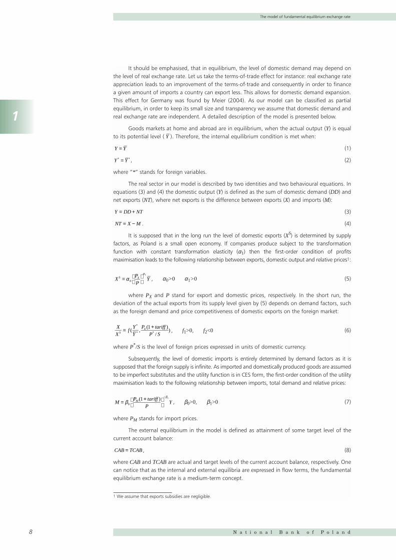
Corresponding to the presented model, one can see that various combinations of the domesticdemand and the real exchange rate may result in different types of disequilibria. These disequilibria aswell as the fundamental equilibrium values of the exchange rate and the domestic demand are illustratedin Figure 1. This diagram provides several interesting conclusions. Firstly, if the exchange rate deviatesfrom its equilibrium level, it would give rise to serious macroeconomic imbalances in the form of largeand persistent current account surpluses or deficits and/or excessive or depressed levels of the domesticdemand. Secondly, in order to restore the equilibrium of the economy, it is essential to match both theexchange rate and the domestic demand policies. This means that setting the exchange rate at the QFEER

level (see equation 29) must be accompanied by an adjustment of the domestic demand to the levelstated in the equation (28). Otherwise, the economy will not be in the equilibrium. Finally, correspondingto Figure 1 four cases of disequilibria can be distinguished, each one represented by a relevant quadrant.These four cases are characterised below.

The first quadrant might represent the United States in the early 1980s when a major fiscalexpansion contributed to the excessive domestic demand and to the significant deterioration in the UScurrent account balance (see Frankel, Froot 1986). A mixture of the dollar depreciation and a restrictivedemand policy would have been the remedy. Another example is Mexico in 1994, just before the crisis.A slightly different dilemma had to be faced by the Western European countries, especially the UnitedKingdom, Italy and Spain, in the early 1990s. They were in the second quadrant, i.e. they suffered fromdepressed levels of output and a deterioration of their current-account balances. This was mainly due tothe pursuit of excessively tight monetary policies that resulted from the peg of their currencies to theGerman mark. Consequently, the currencies of these three countries were highly overvalued, whichentailed ERM crisis of 1992/1993 (see Driver, Wren-Lewis 1998). The third quadrant characterises theposition of Japan in 1993–1994. The considerable current account surplus required real appreciation ofthe yen. Moreover, expansionary policies were advisable to increase the weak domestic demand. Althoughthese events occurred later, the effects were limited. Finally, the forth quadrant can represent Ireland in thelate 1990s, which was characterised by the positive current account balance and overheated domesticdemand. In order to restore the equilibrium, appreciation of the real exchange rate was recommended.

Q f DD g DDFEER IE FEER EE FEER= =( ) ( )

DD DD R ie DD ee DDFEER = ∈ − ={ : ( ) ( ) }0

∂∂

<Q

DD0Q ee DD= ( ,...

Domestic Demand

Real

exc

hang

e ra

te

DDFEER

IB

EB

Istrong demand

current account deficit

IIweak demand

current account deficitIIIweak demand

current account surplusIV

strong demandcurrent account surplus

QFEER

Figure 1Domestic demand and real exchange rate

Source: adopted from Rosenberg (1996, p. 32).

12

2

Three inputs of the fundamental equilibrium exchange rate model


2 Three inputs of the fundamental equilibrium exchange rate model

The model presented in the previous section is an extended version of the popular IMFapproach developed by Bayoumi and Faruqee (1998). As stated by the authors, the level of thefundamental equilibrium real exchange can be calculated in three steps. Firstly, one mustexogenously assume the level of the target current account balance. Secondly, it is necessary toestimate the level of the so-called underlying current account, i.e. the current account balance thatwould be observed if the output gaps at home and abroad were null and if past changes in the realexchange rate were taken into account. Finally, one must compute the level of the real exchangerate that would equalise the underlying and target levels of the current account. The procedurepresented in this paper differs from the one proposed by the IMF in this sense that the domesticoutput gap is endogenous, more precisely it depends on the level of the exchange rate and thedomestic demand (see equations 3 and 21). This modification implies that one must estimate thelevels of the domestic demand and the exchange rate which would guarantee the existence of theinternal and external equilibria.

In compliance with the proposed methodology, the calculations of the fundamental equilibriumexchange rate require three inputs. Firstly, one must estimate (or calibrate as in Bayoumi and Faruqee1998) unknown coefficients of the foreign trade model described by the relationships (5)–(7) and(12)–(13). Then, on the basis of this model the effects of the demand and the real exchange ratechanges on the net exports and the trade balance can be simulated. Secondly, the unobservable levelsof the potential output at home and abroad must be assessed in order to quantify the internaldisequilibrium. Thirdly, it is necessary to calculate the target level of the current account balance thatwould explicitly describe the external disequilibrium. This section outlines these three issues.

2.1. Foreign trade model

This point presents the results of the estimation of parameters that are present in the foreigntrade model, which is described by the equations (5)–(7) and (12)–(13). The estimation wasperformed on the basis of quarterly data for the period from the first quarter of 1995 until the thirdquarter of 2004, which translates into 39 quarterly observations. The techniques of non-stationarytime series analysis were applied. The estimation has been conducted in two stages. First, on thebasis of the Johansen (1988, 1991) and Hansen-Phillips (1990) methods, four long-termrelationships were found. The choice of these methods was motivated by the results of my earlierresearch on small-sample properties of various models of cointegration (see Rubaszek 2004c)4.Subsequently, the short term dynamics were obtained within the error correction framework. Theresults were as follows.

2.1.1. Export and import volumes of goods and services

As specified in the relationship (5), the long-run supply of exports depends on the ratio ofexport to domestic prices. After a log-linearisation of the equation (5) the Hansen-Phillips procedurewas applied. The results:

4 On the basis of Monte Carlo simulations I investigated statistical properties of different estimators of cointegrating vectors. Ifound that for endogenous regressors Johansen and Hansen-Phillips estimators are unbiased while the OLS one is biaseddownward. Moreover, it turned out that the OLS estimator is the most effective, while the Johansen one was the least effective.

2



5 (30)

imply that the elasticity of transformation equals α1=0.69. The addition of a trend function into the groupof the independent variables aimed to capture in the model the phenomena such as integration with theEuropean Union, liberalisation of trade, inflow of foreign direct investments and other factors, which arediscussed by Mroczek and Rubaszek (2003, 2004). The residual analysis, namely ADF=-3.49 (p=0.00)and LC=0.18 (p=0.20) (see. Hansen, 1992), indicate that the relationship (30) is a cointegrating one.

The short-term dynamics of the volume of Polish exports depends on the demand factors,namely foreign demand and price competitiveness of Polish exports on the foreign markets (see eq. 6).The foreign variables are represented by a weighted sum of the foreign output, foreign GDPdeflators and the bilateral exchange rates, where weights are proportional to the respectivecounties’ share in the Polish foreign trade (see Table 1). The estimation results were as follows:

, (31)

where ectX is the error correction term, i.e. the difference between the actual and fitted values inthe relationship (30). Short-run demand elasticity of exports is moderate and amounts to 1.70. Thestatistical properties of the model (31) seem to be plausible, namely: R2=0.63, LM(4)=2.6[p=0.62] and JB(2)=1.44 [p=0.49].

The import volume, both in the long and short-term horizons, depends solely on the demandfactors, i.e. the ratio of import to domestic prices and the level of the domestic activity (see equation7). After a log-linearisation of the equation (7) the Hansen-Phillips procedure was applied. The results:

(32)

imply that the elasticity of substitution equals β1=0.85. The addition of a trend function into thegroup of the independent variables was motivated by the same phenomena as in the case ofequation (30). The residual analysis, namely ADF=-2.68 (p=0.01) and LC=0.27 (p=0.20),demonstrate that the relationship (32) is cointegrating one.

The short-term dynamics of the volume of imports:

, (33)

5 Lowercase letters stand for the logarithms of capital letters, e.g. y = ln(Y). The numbers in the parentheses denote standarddeviations of the estimated coefficients.

Table 1Countries’ share in the Polish foreign trade (%)

1995 2002 1995–2002 Weights

Germany 32.5 28.3 30.0 47.0

Italy 6.7 6.9 7.4 11.6

France 4.2 6.5 5.5 8.6

United Kingdom 4.6 4.5 4.5 7.1

Netherlands 5.1 4.0 4.4 6.8

Czech Rep. 3.1 3.6 3.4 5.3

United States 3.3 3.0 3.3 5.1

Sweden 2.8 2.9 2.7 4.3

Belgium 2.5 3.0 2.7 4.2

Total 64.8 62.7 63.9 100

Source: OECD.

14

2



indicate, that the demand elasticity is moderate and amounts to 1.74. Statistical properties of themodel (33), namely R2=0.67, LM(4)=8.7 [p=0.07] and JB(2)=0.23 [p=0.89], are acceptable.

2.1.2. Export and import prices of goods and services

The relationships (12) and (13) specify export and import prices which are the weightedaverage of the domestic and foreign prices. As there are sound economic reasons that in the systemof the four variables:

(34)

all price indices may be endogenous6 and there could be more than one cointegrating vector7, theJohansen procedure was chosen. Firstly, the optimum lag of the unrestricted VAR was tested.According to the Akaike, Schwarz and Hannan-Quinn information criteria, four lags should beincluded in the model. Then the number of cointegrating vectors was investigated on the basis ofthe Johansen’s (1991) trace and maximum eigenvalue tests. The results, which are presented inTable 2, indicate that there are two cointegrating vectors, which have been interpreted in terms ofthe relationships (12) and (13).

Even though the restrictions on the cointegrating vectors that derive from the equations (12)and (13) were rejected by the data, the values of estimated elasticities:

(35)

(36)

are in line with the economic intuition that Poland, as a small open economy, is in about 80% aprice taker country.

The short-term dynamics of the transaction prices was estimated independently within theerror correction framework. In both equations, constant terms were excluded and homogeneityrestrictions were imposed. The results were as follows:

(37)

. (38)

Statistical properties of both models, i.e. R2=0.64, LM(4)=13.9 [p=0.01], JB(2)=1.1[p=0.58] for the equation (37) and R2=0.66, LM(4)=14.5 [p=0.01], JB(2)=3.6 [p=0.16] for therelationship (38), seem to be acceptable, despite the occurrence of the residual autocorrelation.

p p p p sX M ( )* −[ ]

Table 2Cointegration trace test

Zero hypothesis Trace test Probability Max. Eigenvalue test Probability

r=0 75.3 0.00 37.0 0.00

r≤1 38.3 0.00 28.4 0.00

r≤2 9.9 0.29 8.6 0.32

r≤3 1.3 0.26 1.3 0.26

Source: own calculations.

6 Import and export prices are endogenous according to the equations (12) and (13). If pass-through is different fromnull, then domestic prices react to changes in import prices. Finally, nominal exchange rate component in expression p*–smay be dependent on terms of trade or domestic price.7 Two cointegrating vectors are given in (12) and (13). The third cointegrating vector may exist if purchasing power parityhypothesis is true, i.e. if p–p*+s~I(0).

2



2.1.3. Simulations

On the basis of the presented model an impact of the domestic as well as foreign demandand the real exchange rate on the net exports and the trade balance has been calculated. This pointdiscusses the results of those simulations.

First, let us focus on the effects of a rise in the domestic demand by 1% of GDP, under theassumption that the levels of all other exogenous variables remain unchanged. This expansion ofthe domestic demand increases the output and, according to the equation (33), leads to highervolume of imports. The total effect on the output is less than one-to-one, as the net exportdeteriorates (see equations 3 and 4). As the short-term demand elasticity of imports is 1.74 (seeequation 33) and the imports share in GDP amounts to 37.4%8, it can be calculated that a cyclicalrise in the domestic demand by 1% of GDP leads to immediate increases in the output and importsby 0.61% and 1.06%9, respectively. This translates into a decrease in the net exports by 0.39% ofGDP. The impact of this shock on the trade balance is negative and amounts to 0.44% of GDP.

The second impulse that was introduced to the model was defined as a cyclical expansion ofthe foreign output by 1%. This shock increases domestic exports by 1.7% (see equation 31). As theexport share in GDP is 35.9%10, it can be calculated that a cyclical rise in foreign output by 1%leads to increases in domestic output and imports by 0.37% and 0.64%, respectively. This time, netexports improve by 0.37% of GDP. All the changes are instantaneous.

Finally, the response of the model to the exchange rate shock, defined as a 10% permanentreal depreciation of the zloty, was analysed. Within a system made up of identities (3), (4), (9), (10),(11) and behavioural equations (31), (33), (37), (38) the impact of such impulse on export andimport prices and volumes can be calculated. The results presented in Table 3 indicate that in fiveyears’ horizon the net exports improve by about 2.9% of GDP, where the two thirds of theadjustment occurs in the two initial years.

2.2. Internal equilibrium

The internal equilibrium is defined to occur when the actual output equals its potential level (seeequation 1). In this sense, internal balance implies that the goods markets clear11. In order to quantifythe internal disequilibrium it is necessary to assess the unobservable level of potential output. Theproblem is not trivial, as there is no unique and commonly accepted method of measuring thisquantity. In practice, there exist a large number of various approaches to calculate the level ofpotential output (see Table 4). It appears, however, that the different methods lead to generally unlikeresults. The correlation of output gaps is low, the methods imply various turning points and the

8 NBP estimates for 2004.9 A perceptive reader may notice that 1.06=1.74*0.61.10 NBP estimates for 2004.11 Some authors (e.g. Williamson 1994) define internal equilibrium in terms of the labour market, namely if the actualunemployment equals the NAIRU (non-accelerating rate of unemployment).

Table 3An impact of 10% permanent depreciation of the RER on foreign trade

Years1 2 3 4 5 LR

Volume of exports 2.0 0.7 0.9 0.7 0.4 4.9

Volume of imports -2.0 -0.6 -0.4 -0.2 -0.2 -3.4

Export prices 5.6 1.4 0.5 0.1 0.0 7.7

Import prices 6.8 0.7 0.4 0.2 0.1 8.4

Net exports (% GDP) 1.5 0.5 0.5 0.3 0.2 2.9

Trade balance (% GDP) 1.1 0.8 0.6 0.3 0.2 3.1


16

2



volatility of output gaps is dissimilar. This was illustrated by Chagny and Dopke (2001), who comparedthe potential output for the euro area economy calculated on the basis of different methods.

In this paper the output gap data for Poland and for foreign countries were calculated on thebasis of the Cobb-Douglas production function. In comparison to other methods, the productionfunction approach seems to be the most intuitive. Moreover, the main advantages of this methodare its strong economic foundations. The data of the output gap for Poland were taken from thestudy by Gradzewicz and Kolasa (2005) and for the Polish main trading partners, which are listedin Table 1, from the OECD database. The values for the foreign countries were estimated also onthe basis of the Cobb-Douglas production function, according to the methodology presented inGiorno et al. (1995) and can be found in the OECD Outlook No. 76 (2004).

2.3. External equilibrium

The most controversial part in the presented model refers to the level of target currentaccount balance (TCAB). It appears that the estimates of the fundamental equilibrium exchangerate are very sensitive with respect to the value of the TCAB. This is especially true for relativelyclosed economies, where even small changes of the current account balance require substantialexchange rate adjustments. This controversy also stems from the fact that there is no generallyaccepted economic theory that could be a guideline in the calculations of the TCAB level. This pointbriefly discusses different approaches to calculating a target current account level.

The first method to assess a current account dynamics is based on the intertemporal approach. Theinitial theoretical models, however, have failed to reflect the observed current account changes. Thesemodels predict excessive current account changes in response to various shocks. For example, Obstfeldand Rogoff (1996) presented a simple model that in the steady-state produced the trade surplus equal

Tabela 4Methods to estimate the output gap

• Peak-to-peak; linear detrending; robust detrending; phase average detrending; • Hodrick-Prescott filter; Beverige-Nelson decomposition; unobservable component

or band-pass filter

• Survey data

• Okun’s law; production function approaches, long-run restriction models (SVAR)

• Multivariate Beverige Nelson decomposition, multivariate Hodrick-Prescott filter,multivariate unobservable component method

Non-Structuralmethods

Direct measures

Structural methods

Multivariate methods

Source: adapted from Chagny and Dopke (2001).

Poland Trading partners

-2.5

-2.0

-1.5

-1.0

-0.5

0.0

0.5

1.0

1.5

2004200320022001200019991998199719961995

Figure 2Output gap in Poland and in its main trading partners

Source: Gradzewicz and Kolasa (2005) and OECD Outlook (2004).

2



to 45% of GDP and the foreign debt stabilised at a level that was equal to 15-year value of the GDP. Ifthis basic model, however, is extended for default risk, costs of adjustment or non-Ricardian consumers,etc. then it may generate the results that are closer to reality. Bussiere, Fratzscher and Muller (2004), forinstance, developed a model with two types of consumers: the non-Ricardians, who consume their entiredisposable income, and the Ricardians, who maximise the utility function with habit formations. Thesolution of this theoretical model leads to a parsimonious specification, where the current accountbalance depends on its lagged values and variables such as relative income, relative investment and fiscalbalance. The authors claim, that the estimation results provide credible explanation of the past changesin the current account balances for 33 countries included in the sample. In case of Poland, the authorshave found that in 2002 the current account balance should amount to -2.4 or -5.2% of GDP, dependingon the method of estimation. It should be added here, that even though the intertemporal approachmodels seem to be theoretically plausible, their empirical properties still require further investigation.

The second approach, which was proposed by Debelle and Faruquee (1998), was christened“macroeconomic balance approach”. In compliance with this method the current account balanceis regressed in respect to the long-term determinants of savings and investments such as the stageof economic development, demographics and macroeconomic policies. The theoretical value of thisregression, conditional on the assumption that the explanatory variables are in their medium-termequilibrium, is supposed to equal the level of the TCAB. In case of the Central and Eastern Europeancountries, the macroeconomic balance approach was applied by Doisy and Herve (2001). Theauthors found that the level of the TCAB for Poland in 1998 amounted to -2.6 or -3.2% of GDP,depending on the assumption related to the medium-term level of the budget deficit. The maindisadvantage of the macroeconomic balance approach is that in empirical applications, a highshare of the TCAB variability across countries is justified not by explanatory variables, but by thecountry specific constants included in the panel regressions.

The third approach to calculating the target current account balance is based on the solvencycriterion. This method defines the TCAB as the value of the current account balance that would stabilisethe net foreign debt at its steady-state value. That implies that the TCAB calculations require an assessmentof the steady-state level of the net foreign debt. Ades and Kaune (1997), for instance, calibrated “defaultrisk” model, which had been proposed by Obstfeld and Rogoff (1996), in order to calculate the maximumaccessible net foreign debt for a group of developing countries. They computed that Polish net foreigndebt should not exceed 55.4% of GDP. In other case it would be more profitable for Poland to defaultthan to service this debt. The more recent calculations of the European Commission (European Economy,2002, p. 127), which are based on the panel regression of the foreign debt on the level of GDP per capitaand the degree of openness, indicate that a theoretical value of Polish debt amounts to 39% of GDP. Thisis not contradictory to the results presented by Pattillo et al. (2002) who estimated that for developingcountries, the debt level exceeding 35–40% of GDP has a negative impact on the GDP growth. Taking theabove considerations into account, the assumption that the actual value of the Polish net foreign debt,which at the end of 2003 amounted to 42.3% of GDP12, is in the steady-state seems realistic.

If a country maintains its ratio of the net foreign debt (NFD) to GDP at a constant level, thisdoes not imply that the current account balance is null. According to Milesi-Feretti and Razin(1996), the level of the current account balance that stabilises this ratio is equal to:

.13

(39)

If the expression in brackets in the equation (39) is plausibly assumed to equal 7%, one couldcalculate that the current account deficit that would stabilise the net foreign debt of Poland at theactual level equals to 3.0% of GDP. This value is set as the level of the TCAB in further calculations.It can be noted here that this level is not inconsistent with the results of the studies based on theintertemporal and macroeconomic balance approaches.

CAB

Y

NFD

Y

S

t

Y

t

NFD

Y

Q

t

Y

t

P

tN N

N

N

= − ∂∂

+ ∂∂

= − ∂∂

+ ∂∂

+ ∂∂

(ln( ) ln( )

) (ln( ) ln( ) ln( )

)*

12 On the basis of international investment position statistics, www.nbp.pl.13 It is assumed here that all foreign assets and liabilities are denominated in foreign currency.

18

2



Finally, let us assume the steady-state values for the balances on income and transfers (seeequations 8 and 9). If the nominal interest rate on the net foreign debt (i) equals to 5%, then themedium-term value of the balance on income equals to -2.2% of GDP, according to the relationship:

. (40)

In case of balance on transfers, taking the inflows of the EU funds enlarged by transfers ofPoles working abroad into account, it is possible to assume that its medium-term level equals to3.5% of GDP (cf. Centrum Europejskie Natolin, 2003, p. 39). Consequently, according to (9) we cancalculate, that the target level of the trade balance (TCAB_TB) amounts to -4.3% of GDP.

CAB INC i NFD_ *=

3

The results


3 The results

The previous sections have presented the foreign trade model and discussed issuesconcerning the internal and external equilibria. These three issues combined together allow us tocalculate the level of the fundamental equilibrium exchange rate for the zloty. It should be stressedthat the plausibility of the final results depends on the credibility of these three inputs.

This section demonstrates the method of estimating the fundamental equilibrium exchangerate. Additionally, the sensitivity analysis of the final results is performed.

3.1. The level of the zloty’s fundamental equilibrium exchange rate

Calculations of the fundamental equilibrium levels of the exchange rate and the domesticdemand are performed in two steps. Firstly, one must calculate the values of the trade balance andthe net exports if output gaps were null and past changes of the real exchange rate materialised.These levels, which are referred to as the adjusted trade balance (ACAB_TB) and the adjusted netexports (ANT), can be calculated according to the following formulas:

(41)

, (42)

where and :

, (43)

, . (44)

Expressions and denote materialised impact of i-th period lagged realexchange rate change ( ) on the trade balance and the net exports, respectively. Consequently,one can calculate that the adjusted output gap (AGAP) equals to:

, (45)

where the GAP is the difference between the actual and potential output:

. (46)

The results, which are presented in Table 5, indicate that in 2004 the ACAB_TB was lower than theCAB_TB by 0.2% of GDP and the difference between AGAP and GAP amounted to -0.3% of GDP. Thisdifference is the sum of the two opposite effects. On the one hand, low foreign demand (see Figure 2)indicates that the adjusted values should be higher than the actual ones. On the other, the immaterialisedeffects of the zloty’s appreciation, which occurred in 2004, translate into a fall of ACAB_TB and AGAP.

In the second stage, it is required to estimate the extent of the domestic demand and thereal exchange rate changes necessary to equalise the adjusted values of the trade balance and theoutput gap to their target levels. In section 2 it has been shown how the control variables, i.e. the

GAP Y Y= −

AGAP DD ANT Y GAP ANT NT= + − = + −

∆qt i−

ϑ i t iq∆ −θi t iq∆ −

ϑ ϑ=→∞limi

iϑ it

t jj

i NT

q= ∂

∂ −=∑

0

θ θ=→∞limi

iθit

t jj

i CAB TB

q= ∂

∂ −=∑ _

0

ϑ iθi

ANT NTNT

yy y qt t

t

tt t i t i

i

= + ∂∂

− + − −=

∞

∑** *( ) ( )ϑ ϑ ∆

0

ACAB TB CAB TBCAB TB

yy y qt t

t

tt t i t i

i

_ __

( ) ( )** *= + ∂

∂− + − −

=

∞

∑ θ θ ∆0

20

3

The results


domestic demand and the real exchange rate, influence the current account balance and thedomestic output. It has been shown, that a rise in the domestic demand by 1% of GDP leads to anincrease of the GAP by 0.61% of GDP and to a deterioration of the CAB_TB by 0.44% of GDP. Theimpact of the real exchange changes has been presented in Table 3. Thus, it can be calculated, that:

(47)

. (48)

As the adjusted values of the output gap and the trade balance in the equilibrium are equalto their target levels, the required changes amount to:

(49)

(50)

On the basis of the expressions (47)–(50) on can see that the deviations of the controlvariables from its fundamental equilibrium levels are the solution of the system:

,(51)

which is given by:

.(52)

Substitution of the respective values from Table 5 into the expression (52):

(53)

leads to the final results, which imply that in the forth quarter of 2004 the quarterly average realeffective exchange rate of the zloty was undervalued by 4.3% and the domestic demand wassubdued by 3.1% of GDP14. As this result is conditional on a set of assumptions, it should beinterpreted cautiously. This issue is discussed below.

3.2. Sensitivity analysis

The results in the previous point indicate that in the forth quarter of 2004 the zloty’s rate wasundervalued by 4.3%. It should be emphasised, however, that the plausibility of this result dependson the plausibility of three inputs that were outlined in the section 2. It can be said that theestimated fundamental equilibrium exchange rate is conditional on the assumptions concerning thelevel of the output gaps at home and abroad, and the target trade balance. This point discusseshow these assumptions affect the final result.

( ) / . .

. .

.

.

.

.

DD DD Y

q q

FEER

FEER

−−

=

−− −

−

=

0 98 0 94

1 39 1 93

0 6

2 7

3 1

4 3

( ) / . .

. .

/

( _ _ ) /

DD DD Y

q q

AGAP Y

TCAB TB ACAB TB Y

FEER

FEERN

−−

=

−− −

−−

0 98 0 94

1 39 1 93

−−

=−

− −

−−

AGAP Y

TCAB TB ACAB TB Y

DD DD Y

q qN

FEER

FEER

/

( _ _ ) /

. .

. .

( ) /0 61 0 29

0 44 0 31

∆CAB TB TCAB TB ACAB TB_ _ _= −

∆AGAP AGAP= −

∆ ∆ ∆ACAB TB Y DD Y qN_ . .( ) = − ( ) −0 44 0 31

∆ ∆ ∆AGAP Y DD Y q( ) = ( ) −0 61 0 29. .

Table 5Balance on goods and services and output gap in Poland in 2004

CAB_NT Domestic output gap(%GDP) (%GDP)

Actual value -1.4 -0.3

Adjusted value -1.6 -0.6

Adjustment due to: foreign output gap 0.9 0.9

past changes of real exchange rate -1.2 -1.2

Target value -4.3 0.0

Source: NBP, own calculations.

14 These results relate to the annual values of domestic demand.

3

The results


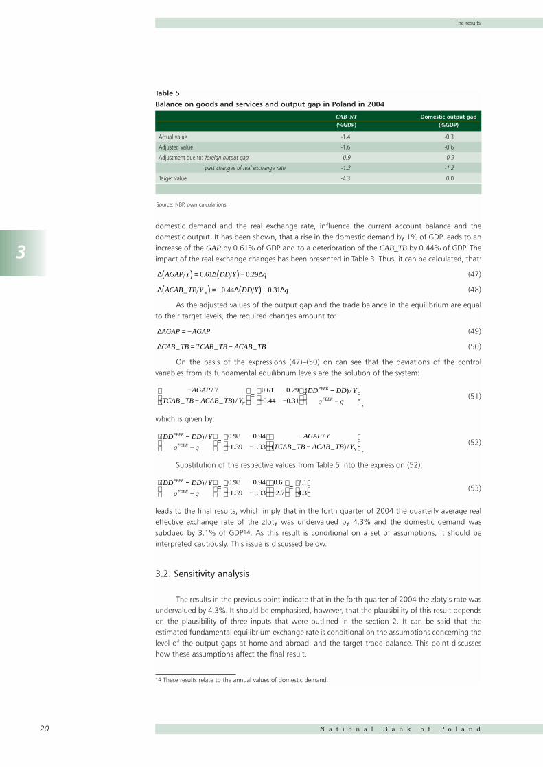
3.2.1. Foreign output gap

First, it is investigated how the foreign output gap assumptions affect the final results. Animpact of an increase of the assumed level of the foreign output gap by 1% of GDP on the finalresults is calculated. The analysis is conducted by comparing the solutions of the baseline scenarioto the scenario with higher external output gap, which is referred to as scenario 1. In the presentedmodel, this change in assumptions influences the level of the adjusted values of domestic outputgap and trade balance. The calculated multipliers indicate that the AGAP and the ACAB_TB wouldbe lower by 0.36 and 0.37% of GDP, respectively. According to the equation (52) the final resultschange by:

, (54)

where and are the fundamental values of the domestic demand and the realexchange rate in scenario 1. As a result, if the true foreign output gap was higher than the baselinevalue by 1% of GDP, the fundamental equilibrium exchange rate would be 1.2% weaker. Therelationship between the assumed level of foreign output gap and the scale of the zloty’smisalignment in the forth quarter of 2004 is presented in Figure 3. It can be seen there, that if thetrue foreign output gap in 2004 was null15, in the fourth quarter of 2004 the zloty wasundervalued by 1.3%.

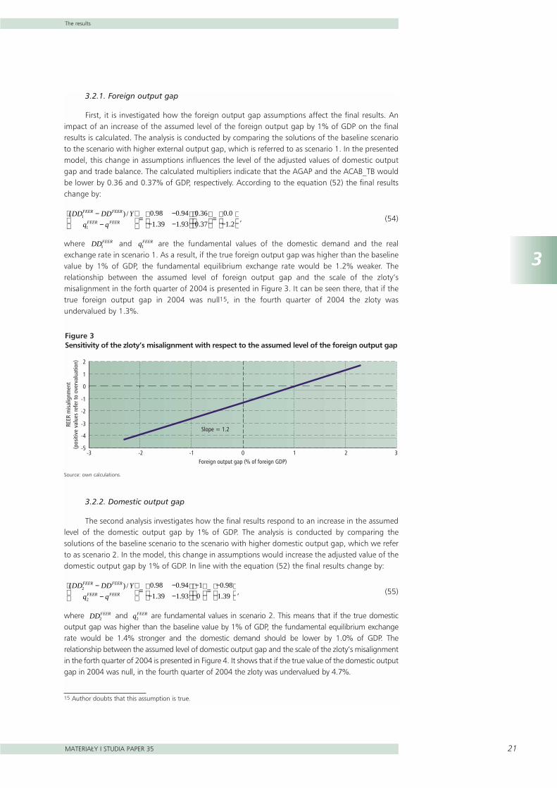
3.2.2. Domestic output gap

The second analysis investigates how the final results respond to an increase in the assumedlevel of the domestic output gap by 1% of GDP. The analysis is conducted by comparing thesolutions of the baseline scenario to the scenario with higher domestic output gap, which we referto as scenario 2. In the model, this change in assumptions would increase the adjusted value of thedomestic output gap by 1% of GDP. In line with the equation (52) the final results change by:

, (55)

where and are fundamental values in scenario 2. This means that if the true domesticoutput gap was higher than the baseline value by 1% of GDP, the fundamental equilibrium exchangerate would be 1.4% stronger and the domestic demand should be lower by 1.0% of GDP. Therelationship between the assumed level of domestic output gap and the scale of the zloty’s misalignmentin the forth quarter of 2004 is presented in Figure 4. It shows that if the true value of the domestic outputgap in 2004 was null, in the fourth quarter of 2004 the zloty was undervalued by 4.7%.

qFEER2DDFEER

2

( ) / . .

. .

.

.

DD DD Y

q q

FEER FEER

FEER FEER

2

2

0 98 0 94

1 39 1 93

1

0

0 98

1 39

−−

=

−− −

−

=−

qFEER1DDFEER

1

( ) / . .

. .

.

.

.

.

DD DD Y

q q

FEER FEER

FEER FEER

1

1

0 98 0 94

1 39 1 93

0 36

0 37

0 0

1 2

−−

=

−− −

=−

15 Author doubts that this assumption is true.

-5

-4

-3

-2

-1

0

1

2

-3 -2 -1 0 1 2 3Foreign output gap (% of foreign GDP)

Slope = 1.2

REER

misa

lignm

ent

(pos

itive

val

ues

refe

r to

over

valu

atio

n)

Figure 3Sensitivity of the zloty’s misalignment with respect to the assumed level of the foreign output gap


22

3

The results


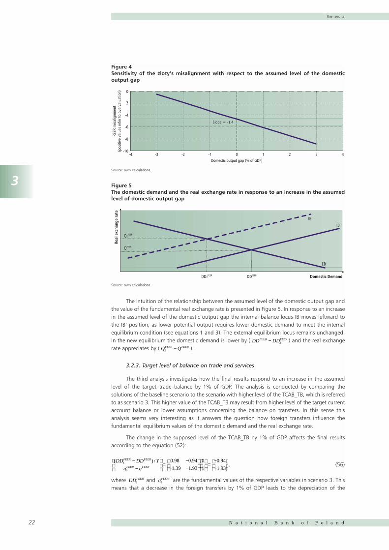
The intuition of the relationship between the assumed level of the domestic output gap andthe value of the fundamental real exchange rate is presented in Figure 5. In response to an increasein the assumed level of the domestic output gap the internal balance locus IB moves leftward tothe IB’ position, as lower potential output requires lower domestic demand to meet the internalequilibrium condition (see equations 1 and 3). The external equilibrium locus remains unchanged.In the new equilibrium the domestic demand is lower by ( ) and the real exchangerate appreciates by ( ).

3.2.3. Target level of balance on trade and services

The third analysis investigates how the final results respond to an increase in the assumedlevel of the target trade balance by 1% of GDP. The analysis is conducted by comparing thesolutions of the baseline scenario to the scenario with higher level of the TCAB_TB, which is referredto as scenario 3. This higher value of the TCAB_TB may result from higher level of the target currentaccount balance or lower assumptions concerning the balance on transfers. In this sense thisanalysis seems very interesting as it answers the question how foreign transfers influence thefundamental equilibrium values of the domestic demand and the real exchange rate.

The change in the supposed level of the TCAB_TB by 1% of GDP affects the final resultsaccording to the equation (52):

, (56)

where and are the fundamental values of the respective variables in scenario 3. Thismeans that a decrease in the foreign transfers by 1% of GDP leads to the depreciation of the

qFEERR3DDFEER

3

( ) / . .

. .

.

.

DD DD Y

q q

FEER FEER

FEER FEER

3

3

0 98 0 94

1 39 1 93

0

1

0 94

1 93

−−

=

−− −

=−−

Q QFEER FEER2 −

DD DDFEER FEER− 2

-10

-8

-6

-4

2

0

-4 -3 -2 -1 0 1 2 3 4Domestic output gap (% of GDP)

Slope = -1.4

REER

misa

lignm

ent

(pos

itive

val

ues

refe

r to

over

valu

atio

n)

Figure 4Sensitivity of the zloty’s misalignment with respect to the assumed level of the domesticoutput gap


Domestic Demand

Real

exc

hang

e ra

te

DDFEERDD2FEER

IB

IB’

EB

Q2FEER

QFEER

Figure 5The domestic demand and the real exchange rate in response to an increase in the assumedlevel of domestic output gap


3

The results


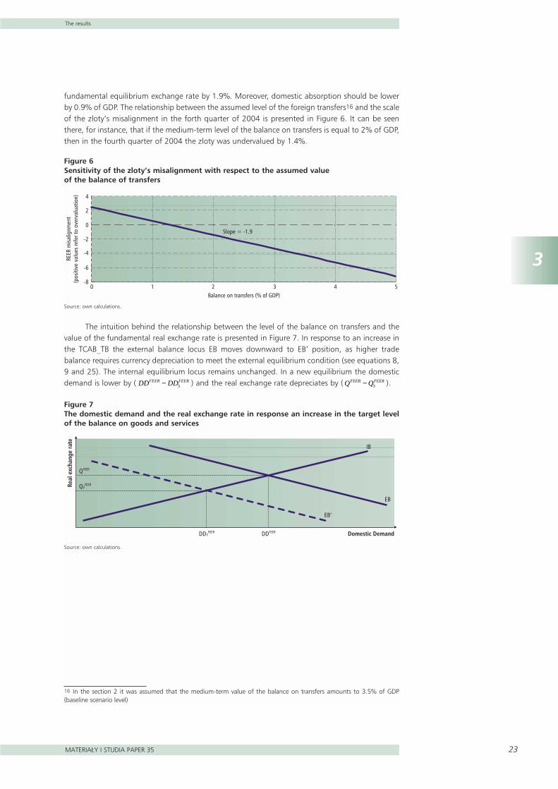
fundamental equilibrium exchange rate by 1.9%. Moreover, domestic absorption should be lowerby 0.9% of GDP. The relationship between the assumed level of the foreign transfers16 and the scaleof the zloty’s misalignment in the forth quarter of 2004 is presented in Figure 6. It can be seenthere, for instance, that if the medium-term level of the balance on transfers is equal to 2% of GDP,then in the fourth quarter of 2004 the zloty was undervalued by 1.4%.

The intuition behind the relationship between the level of the balance on transfers and thevalue of the fundamental real exchange rate is presented in Figure 7. In response to an increase inthe TCAB_TB the external balance locus EB moves downward to EB’ position, as higher tradebalance requires currency depreciation to meet the external equilibrium condition (see equations 8,9 and 25). The internal equilibrium locus remains unchanged. In a new equilibrium the domesticdemand is lower by ( ) and the real exchange rate depreciates by ( ).Q QFEER FEER− 3DD DDFEER FEER− 3

-8

-6

-4

-2

0

2

4

0 1 2 3 4 5Balance on transfers (% of GDP)

REER

misa

lignm

ent

(pos

itive

val

ues

refe

r to

over

valu

atio

n)

Slope = -1.9

Figure 6Sensitivity of the zloty’s misalignment with respect to the assumed valueof the balance of transfers


Domestic Demand

Real

exc

hang

e ra

te

DDFEERDD3FEER

EB

IB

EB’

QFEER

Q3FEER

Figure 7The domestic demand and the real exchange rate in response an increase in the target levelof the balance on goods and services


16 In the section 2 it was assumed that the medium-term value of the balance on transfers amounts to 3.5% of GDP(baseline scenario level)

24

4

Summary


4Summary

In May 2004 Poland joined the European Union and in subsequent years it is supposed toenter the European Monetary Union. Common monetary policy offers long-term benefits such aslower risk premium, fall of transaction costs, lower currency risks etc. In the short-term horizon,however, the EMU accession may be a challenge for Polish economy, especially if the conversionrate is set at a misaligned level. This paper attempted to investigate this issue. The partialequilibrium model was proposed. This model was used to calculate the level of the fundamentalequilibrium rate of the zloty. The results suggest that in the forth quarter of 2004 the zloty wasundervalued by 4.3%. As these results depend on a set of assumptions the sensitivity analysis wasperformed. It has been found out that in this period, in case of a low net inflow of the EU transfers,the real exchange rate of the zloty was not misaligned.

It should be emphasised, that apart from the FEER model, there exist other approaches thatcan be used to estimate the level of the equilibrium exchange rate. Let us take for instance themonetary models (Frenkel 1976), the equilibrium model of the exchange rate (Stockman,1987), thebehavioural equilibrium exchange rate model (Clark and MacDonald 1998), the natural realexchange rate model (Stein 1995) and others. The application of these models to calculate theequilibrium level of the zloty can be the issue of further research.

5

References


5References

1. Ades, A. and Kaune, F. (1997): A New Measure of Current Account Sustainability for DevelopingCountries. Goldman-Sachs Emerging Markets Economic Research.

2. Bayoumi, T. and Faruqee, H. (1998): A Calibrated Model of the Underlying Current Account. InFaruqee H., Isard P., ed.

3. Borowski, J., ed. (2004): A Report on the Costs and Benefits of Poland’s Adoption of the Euro.National Bank of Poland.

4. Bussiere, M., Fratzscher, M. and Muller, G. (2004): Current Account Dynamics in OECD and EUAcceding Countries – an Intertemporal Approach. ECB WP No. 311.

5. Centrum Europejskie Natolin (2003): KorzyÊci i koszty cz∏onkostwa Polski w Unii Europejskiej.Warsaw.

6. Chagny, O. and Dopke, J. (2001): Measures of the Output Gap in the Euro-Zone: An EmpiricalAssessment of Selected Methods. Working Paper No. 1053, Kiel Institute of World Economics, Kiel.

7. Clark, P. and MacDonald, R. (1998): Exchange Rates and Economic Fundamentals: AMethodological Comparison of BEERs and FEERs. IMF Working Paper WP/98/67, InternationalMonetary Fund, Washington.

8. Devarajan, S. (1999): Estimates of Real Exchange Rate Misalignment with a Simple General-Equilibrium Model. Chapter VIII in Hinkle L., Montiel P., eds.

9. Debelle, G. and Faruqee, H. (1998): Saving-Investment Balances in Industrial Countries: AnEmpirical Investigation. In Faruqee H., Isard P., ed.

10. Doisy, N. and Herve, K. (2001): The Medium and Long Term Dynamics of the Current AccountPositions i the Central and Eastern European Countries: What Are the Implications for theirAccession to the European Union and the Euro Area? Preliminary version.

11. Driver, R. and Wren-Lewis, S. (1998): Real Exchange Rates for the Year 2000. Institute forInternational Economics, Washington.

12. European Economy No. 3/2002: Public finances in EMU. European Commission, Directorate-General for Economic and Financial Affairs.

13. Faruqee, H. and Isard, P. (1998): Exchange Rate Assessment: Extension of the MacroeconomicBalance Approach. IMF Occasional Paper 167, International Monetary Fund, Washington.

14. Faruqee, H., Isard, P., Kincaid, R. and Fetherston, M. (2001): Methodology for Current Accountand Exchange Rate Assessments. IMF Occasional Paper 209, International Monetary Fund,Washington.

15. Frankel, J. and Froot, K. (1986): The Dollar as a Speculative Bubble: A Tale of Fundamentalists andChartists. NBER Working Paper No. 1854, National Bureau of Economic Research, Cambridge.

16. Frenkel, J. (1976): A Monetary Approach to the Exchange Rate: Doctrinal Aspects and EmpiricalEvidence. „Scandinavian Journal of Economics” vol. 78, p. 200–224.

17. Giorno, C., Richardson, P., Roseveare D. and Van den Noord, P. (1995): Estimating PotentialOutput, Output Gaps and Structural Budget Balances. Working Papers No. 152, EconomicDepartment of OECD, Paris.

26

5

References


18. Goldstein, M. and Khan, M. (19850): Income and price effects in foreign trade. Chapter XXin Jones R., Kenen P. (eds.): Handbook of International Economics. Vol. II, Elsevier SciencePublishers B.V.

19. Gradzewicz, M. and Kolasa, M. (2005): Estimating the output gap in the Polish economy: theVECM approach. IFC Bulletin No. 20.

20. Grossman, G. and Rogoff, K., eds. (1995): Handbook of International Economics. Vol. III.,Elsevier Science Publishers B.V.

21. Hansen, B. (1992): Tests for Parameter Instability in Regressions with I(1) Processes. „Journal ofBusiness and Economic Statistics” vol. 10, s. 321–334.

22. Hansen, B. and Phillips, P. (1990): Statistical Inference in Instrumental Variables Regression withI(1) Processes. „Review of Economic Studies” vol. 57, s. 99–125.

23. Hansen, J. and Roeger, W. (2000): Estimation of Real Exchange Rates. Economic PapersECFIN/534/00-EN, Directorate General for Economic and Financial Affairs, European Commission.

24. Hinkle, L. and Montiel, P. (1999): Exchange Rate Misalignment. World Bank ResearchPublication, Washington.

25. Johansen, S. (1988): Statistical Analysis of Cointegrating Vectors. „Journal of Economic Dynamicsand Control” vol. 12, s. 231–254.

26. Johansen, S. (1991): Estimation and Hypothesis Testing of Cointegrating Vectors in GaussianVector Autoregression Models. „Econometrica” vol. 59, s.1551–1580.

27. Jones, R. and Kenen, P., eds. (1985): Handbook of International Economics. Vol. I and II, ElsevierScience Publishers B.V.

28. MacDonald, R. (2000): Concepts to Calculate Equilibrium Exchange Rates: An Overview.Discussion Paper 3/00, Deutsche Bundesbank.

29. Meier, C. (2004): Investigating the impact of an appreciation of the euro in a smallmacroeconometric model of Germany and the euro area. Kiel WP No. 1204.

30. Milesi-Ferretti, G. and Razin, A. (1996): Sustainability of Persistent Current Account Deficits.NBER Working Paper No. 5467, National Bureau of Economic Research, Cambridge.

31. Mroczek, W. and Rubaszek, M. (2003): Determinanty Polskiego Eksportu i Importu. NBP PaperNo. 161, National Bank of Poland, Warsaw.

32. Mroczek, W. and Rubaszek, M. (2004): Development of the trade links between Poland and theEuropean Union in the years 1992–2002. NBP Paper No. 30, National Bank of Poland, Warsaw.

33. NBH (2002): Adopting the euro in Hungary: expected benefits, costs and timing. NBHOccasional Paper No. 24, National Bank of Hungary, Budapest.

34. Obstfeld, M. and Rogoff, K. (1995): The intertemporal Approach to the Current Account.Chapter 34 in Grossman G., Rogoff K., eds.

35. Obstfeld, M. and Rogoff, K. (1996): Foundations of International Macroeconomics. MIT Press.OECD Economic Outlook No. 76, 2004, OECD, Paris.

36. Pattillo, C., Poirson, H. and Ricci, L. (2002): External Debt and Growth. IMF Working Paper WP/02/69,International Monetary Fund, Washington.

37. Roseberg, M. (1996): Currency Forecasting. IRWIN, Chicago.

38. Rubaszek, M. (2003): Optimal ERM II Central Parity for Polish Zloty. ECB conference „EquilibriumExchange Rates in Accession Countries: Macroeconomic and Methodological Issues” papers.

39. Rubaszek, M. (2004a): A Model Of Balance Of Payments Equilibrium Exchange Rate.Application to the Zloty. „Eastern European Economics” vol. 42, Iss. 5, p. 5–22.

5

References


40. Rubaszek, M. (2004b): Modelowanie optymalnego poziomu realnego efektywnego kursuz∏otego. Zastosowanie koncepcji fundamentalnego kursu równowagi. „Materia∏y i Studia”,Narodowy Bank Polski, Zeszyt nr 175.

41. Rubaszek, M. (2004c): Porównanie w∏aÊciwoÊci statystycznych ró˝nych estymatorów relacjikointegrujàcej metodà symulacji Monte Carlo (A Monte Carlo comparison of statisticalproperties of various methods to estimate cointegrating relationship.). Internal research atWarsaw School of Economics.

42. Stein, J. (1995): The Fundamental Determinants of the Real Exchange Rate of the U.S. DollarRelative to Other G-7 Countries. IMF Working Paper WP/95/81, International Monetary Fund,Washington.

43. Stockman, A. (1987): The equilibrium Approach to Exchange Rates. „Federal Reserve Bank ofRichmond Economic Review” vol. 73 (2), p. 12–30.

44. Williamson, J. (1983): The Exchange Rate System. „Policy Analyses in International Economies”vol. 5, Institute for International Economics, Washington.

45. Williamson, J. (1994): Estimates of FEER. In Williamson J., ed.

46. Williamson, J., ed. (1994): Estimating Equilibrium Exchange Rates. Institute for InternationalEconomics, Washington.

Documents

MATERIA¸Y I STUDIA - ssl.nbp.pl