DEGREE PROGRAMME IN ELECTRICAL ENGINEERING

MASTER’S THESIS

VIRTUAL ANTENNA ARRAY BASED MIMO RADIO

CHANNEL MEASUREMENT SYSTEM AT 10 GHZ

Author Nuutti Tervo

Supervisor Risto Vuohtoniemi

Second Examiner Juha-Pekka Mäkelä

(Technical advisor Veikko Hovinen)

October 2014

Tervo N. (2014) Virtual Antenna Array Based MIMO Radio Channel Measure-ment System at 10 GHz. University of Oulu, Department of Communications Engi-neering, Degree Programme in Electrical Engineering. Master’s Thesis, 58 p.

ABSTRACT

In this thesis, a 10 GHz multiple-input multiple-output radio channel measure-ment system using four port vector network analyzer and virtual antenna arraysin both transmitter and receiver ends is presented. The channel measurement sys-tem measures each single antenna channel separately. The radio propagation en-vironment is assumed to be static during the recordings. As an antenna element,a dual polarized patch antenna with two feeding ports is used. Linear stages andprogrammable stepper motors are utilized to build an XY-gantry to move the an-tenna element in a plane. The stepper motors and the vector network analyzerare controlled by the same measurement control software. The basic principles ofthe control software are also presented along the measurement system.

Three channel measurement scenarios and their initial results are presented toverify the system operation and to demonstrate the system in different cases. Averification measurement is performed in an anechoic chamber to verify that thesystem does not cause internal spurious responses to the results. The next mea-surement is performed in a classroom to demonstrate the multipath propagationenvironment. Furthermore, an indoor wall penetration loss measurement fromthe classroom to another is made to show that the measurement system can alsobe applied for the measurements requiring an accurate antenna shifting betweenthe measurement points. The results measured with this setup can be appliedangular domain algorithms to estimate the direction of arrival and departure,respectively.

Keywords: millimeter-wave, static channel modeling, massive MIMO channelmeasurements.

Tervo N. (2014) Virtuaalista antenniryhmää käyttävä MIMO-radiokanavan mit-tausjärjestelmä 10 GHz:n taajuudelle. Oulun yliopisto, tietoliikennetekniikan osas-to, sähkotekniikan koulutusohjelma. Diplomityö, 58 s.

TIIVISTELMÄ

Tämä diplomityö esittelee moniantenniradiokanavan mittausjärjestelmän, jossamittauslaitteena käytetään vektoripiirianalysaattoria ja kahta virtuaalista ta-soantenniryhmää. Järjestelmä mittaa jokaisen antennielementin välisen kanavanerikseen. Etenemisympäristö on oletettu staattiseksi radiokanavan tallennuksenaikana. Antennielementtinä käytetään kaksoispolaroitua mikroliuska-antennia,jossa on omat syöttöportit molemmille ortogonaalisille lineaarisille polarisaatioil-le. Antennielementtiä siirretään tasossa käyttämällä ohjelmoitavia askelmootto-reita ja lineaariyksiköitä. Kaikkia mittausjärjestelmän laitteita ohjataan samallaohjausohjelmistolla, jonka toimintaperiaate on myös esitetty tässä työssä.

Mittausjärjestelmän toiminta varmistetaan ja sitä demonstroidaan suoritta-malla kanavamittauksia erilaisissa etenemisympäristöissä. Varmennusmittauksetsuoritetaan kaiuttomassa huoneessa, jotta voidaan varmistua siitä, ettei järjes-telmä tuota sisäisiä harhatoistoja, jotka vaikuttaisivat mittaustuloksiin. Monitie-etenemisympäristöä demonstroidaan kanavamittauksilla luokkahuoneessa. Myösluokkahuoneiden välistä etenemisvaimennusta mitataan. Mittaustuloksia voidaankäyttää muodostettaessa erilaisia radiokanavamalleja ja niitä voidaan soveltaamyös aallon tulo- ja lähtökulman estimointiin käyttämällä siihen tarkoitettuja al-goritmeja.

Avainsanat: millimetriaallot, staattisen kanavan mallinnus, massiivi MIMO ka-navamittaukset.

TABLE OF CONTENTS

ABSTRACT

TIIVISTELMÄ

TABLE OF CONTENTS

FOREWORD

LIST OF ABBREVIATIONS AND SYMBOLS

1. INTRODUCTION . . . . . . . . . . . . . . . . . . . . . . . . . . . . . . . . . . . . . . . . . . . . . . . . . 10

2. RADIO CHANNEL CHARACTERISTICS . . . . . . . . . . . . . . . . . . . . . . . . . . . . 132.1. Electromagnetic propagation . . . . . . . . . . . . . . . . . . . . . . . . . . . . . . . . . . . . 13

2.1.1. Plane waves and spherical waves . . . . . . . . . . . . . . . . . . . . . . . . . . 132.1.2. Polarization . . . . . . . . . . . . . . . . . . . . . . . . . . . . . . . . . . . . . . . . . . . . 14

2.2. Propagation in the radio channel . . . . . . . . . . . . . . . . . . . . . . . . . . . . . . . . . 142.2.1. Free space path loss . . . . . . . . . . . . . . . . . . . . . . . . . . . . . . . . . . . . . 142.2.2. Plane wave in the medium . . . . . . . . . . . . . . . . . . . . . . . . . . . . . . . . 152.2.3. Plane wave in the media boundary . . . . . . . . . . . . . . . . . . . . . . . . . 162.2.4. Plane wave in rough surfaces and diffracting edges . . . . . . . . . . . 172.2.5. Fading and shadowing . . . . . . . . . . . . . . . . . . . . . . . . . . . . . . . . . . . 18

2.3. Radio channel modeling . . . . . . . . . . . . . . . . . . . . . . . . . . . . . . . . . . . . . . . . 182.3.1. Frequency and impulse responses . . . . . . . . . . . . . . . . . . . . . . . . . 192.3.2. Delay spread, doppler spread and angular spread . . . . . . . . . . . . . 192.3.3. Deterministic channel models . . . . . . . . . . . . . . . . . . . . . . . . . . . . . 202.3.4. Indoor channel modeling . . . . . . . . . . . . . . . . . . . . . . . . . . . . . . . . . 202.3.5. MIMO channel modeling . . . . . . . . . . . . . . . . . . . . . . . . . . . . . . . . 21

3. RADIO CHANNEL MEASUREMENT SETUP . . . . . . . . . . . . . . . . . . . . . . . . 223.1. VNA based measurement system. . . . . . . . . . . . . . . . . . . . . . . . . . . . . . . . . 22

3.1.1. The proposed measurement setup . . . . . . . . . . . . . . . . . . . . . . . . . . 233.1.2. Scattering parameters . . . . . . . . . . . . . . . . . . . . . . . . . . . . . . . . . . . . 233.1.3. VNA time domain analysis . . . . . . . . . . . . . . . . . . . . . . . . . . . . . . . 24

3.2. Dynamic range of the measurement system . . . . . . . . . . . . . . . . . . . . . . . . 253.2.1. Noise in the measurement system. . . . . . . . . . . . . . . . . . . . . . . . . . 253.2.2. Noise factor, noise figure and noise temperature . . . . . . . . . . . . . 253.2.3. Noise in cascaded radio blocks . . . . . . . . . . . . . . . . . . . . . . . . . . . . 263.2.4. Noise in the VNA . . . . . . . . . . . . . . . . . . . . . . . . . . . . . . . . . . . . . . . 263.2.5. Link budget and external amplifiers . . . . . . . . . . . . . . . . . . . . . . . . 263.2.6. Calibration of the VNA . . . . . . . . . . . . . . . . . . . . . . . . . . . . . . . . . . 28

3.3. Virtual antenna array . . . . . . . . . . . . . . . . . . . . . . . . . . . . . . . . . . . . . . . . . . . 293.3.1. Antenna characteristics . . . . . . . . . . . . . . . . . . . . . . . . . . . . . . . . . . 293.3.2. Dual polarized patch antenna . . . . . . . . . . . . . . . . . . . . . . . . . . . . . 303.3.3. XY-gantry . . . . . . . . . . . . . . . . . . . . . . . . . . . . . . . . . . . . . . . . . . . . . 31

3.4. Wiring of the measurement system . . . . . . . . . . . . . . . . . . . . . . . . . . . . . . . 333.5. Measurement control software . . . . . . . . . . . . . . . . . . . . . . . . . . . . . . . . . . . 33

3.5.1. Controlling the stepper motors . . . . . . . . . . . . . . . . . . . . . . . . . . . . 353.5.2. Controlling the VNA . . . . . . . . . . . . . . . . . . . . . . . . . . . . . . . . . . . . 36

3.5.3. Data format . . . . . . . . . . . . . . . . . . . . . . . . . . . . . . . . . . . . . . . . . . . . 373.5.4. Error control . . . . . . . . . . . . . . . . . . . . . . . . . . . . . . . . . . . . . . . . . . . 383.5.5. User interface . . . . . . . . . . . . . . . . . . . . . . . . . . . . . . . . . . . . . . . . . . 39

4. MEASUREMENT SCENARIOS AND RESULTS . . . . . . . . . . . . . . . . . . . . . . 404.1. Used measurement settings and the system speed performance . . . . . . . . 404.2. Verification measurements in anechoic chamber . . . . . . . . . . . . . . . . . . . . 414.3. Test measurements in classroom . . . . . . . . . . . . . . . . . . . . . . . . . . . . . . . . . 444.4. Wall penetration loss measurements . . . . . . . . . . . . . . . . . . . . . . . . . . . . . . 454.5. Diffraction around a building corner . . . . . . . . . . . . . . . . . . . . . . . . . . . . . . 49

5. DISCUSSION . . . . . . . . . . . . . . . . . . . . . . . . . . . . . . . . . . . . . . . . . . . . . . . . . . . . . 505.1. Evaluation of the system . . . . . . . . . . . . . . . . . . . . . . . . . . . . . . . . . . . . . . . . 505.2. Improvements proposed to the system . . . . . . . . . . . . . . . . . . . . . . . . . . . . 515.3. About the measurements . . . . . . . . . . . . . . . . . . . . . . . . . . . . . . . . . . . . . . . . 52

6. SUMMARY . . . . . . . . . . . . . . . . . . . . . . . . . . . . . . . . . . . . . . . . . . . . . . . . . . . . . . . 54

7. REFERENCES . . . . . . . . . . . . . . . . . . . . . . . . . . . . . . . . . . . . . . . . . . . . . . . . . . . . 55

8. APPENDICES . . . . . . . . . . . . . . . . . . . . . . . . . . . . . . . . . . . . . . . . . . . . . . . . . . . . . 58

FOREWORD

This thesis has been carried out as a part of the 5G radio access solutions to 10 GHzand beyond frequency bands (5G to 10G) project. The project is supported by Broad-com Communications Finland Oy, Elektrobit Wireless Communications Oy, HuaweiTechnologies Oy (Finland) Co. Ltd, Nokia Networks Oy and Finnish funding agencyfor innovation (Tekes). I would like to take this opportunity to thank all the projectpartners for their competence for this work.

I would also like to thank my technical advisor M.Sc (Tech.) Veikko Hovinen forthe great ideas leading to this work. I am graceful for the thesis examiners Lic.Sc(Tech) Risto Vuohtoiemi and D.Sc (Tech.) Juha-Pekka Mäkelä for reading the thesisand advising me in writing. I would also like take this opportunity to thank ProfessorMatti Latva-aho for the trust to my abilities to work here, D.Sc (Tech.) Marko Sonkkifor helping me in the beginning of my work, Anssi Rimpiläinen for implementing themost of the mechanics and M.Sc (Tech.) Claudio Ferreira Dias for the great technicaldiscussion during the work. Furthermore, I would like to thank all the Centre forWireless Communications staff for feeling me welcome to work here.

I would also like to take this opportunity to thank my family and friends for all thesupport I have enjoyed during my University studies. Especially, I would like to thankmy brothers Valtteri and Oskari for the everyday discussion, help and support duringthe studies as well as during the time spend with this thesis. The special thanks goesto my girlfriend Jenny for the sincere support and understanding towards my passionfor science for all the years we have been together.

Oulu, Finland October 24, 2014

Nuutti Tervo

LIST OF ABBREVIATIONS AND SYMBOLS

AC alternating currentAoA angle of arrivalAoD angle of departureDC direct currentDoA direction of arrivalDoD direction of departureGO geometrical opticsGPS global positioning systemGTD geometrical theory of diffractionGUI graphical user interfaceIDFT inverse discrete Fourier transformIF intermediate frequencyIFFT inverse fast Fourier transformIP internet protocolKED knife-edge diffractionLAN local area networkLNA low noise amplifierLOS line-of-sightMCode machine codeMIMO multiple input multiple outputNLOS non-line-of-SightPA power amplifierPDF probability density functionRF radio frequencyRMS root mean squareRT ray tracingRX receiverSCPI standard commands for programmable instrumentsS-parameters scattering parametersTCP/IP transmit control protocol/internet protocolTX transmitterUTD uniform theory of diffractionVNA vector network analyzer3D three dimensional5G fifth generation

a1 signal entering to the 2-port inputa2 signal leaving from the 2-port outputB bandwidthBC coherence bandwidth of the channelBD doppler bandwidthBIF intermediate frequency bandwidthBmeas measurement bandwidthb1 signal reflecting from the 2-port inputb2 signal reflecting from the 2-port output

C(ν) Fresnel cosine integralc0 light speed in vacuumD largest dimension of an antennaDas(θd) absorbing screen diffraction coefficientD(θ, φ) antenna directivityd distancedm distance that the wave has propagated in the mediumd0 reference link distanced1 distance from the TXd2 distance from the RXE(r) electrical field vector as a function of rE0(θ, φ) electrical field vector at distance r = 0e Neper numberecd antenna radiation efficiencyer antenna reflection efficiencye0 total antenna efficiencyFcas total noise figure of cascaded RF-blocksFN noise factorF (ν) knife-edge diffraction coefficientf frequencyfn n:th recorded frequency samplef0 center frequencyG gainGR RX antenna GainGT TX antenna GainG(θ, φ) antenna gainGabs(θ, φ) absolute antenna gainH height of an obstacleH MIMO channel matrixH(f) channel frequency responsehF radius of first Fresnel ellipsoidhij channel coefficient from TX antenna i to RX antenna jhlm impulse response between ports l and mh(t) channel impulse responseI0 Bessel functionj imaginary unitKr Rician K-factork wave numberk complex wave numberkB Bolzmann constantL path lossLfs free space path lossLke knife-edge diffraction lossLm(d) loss in the dielectric mediumLref path loss at the reference distanceNF noise figureNFVNA noise figure of VNA

Nblocks number of RF blocks in the RX chainNFr number of frequency pointsN0 noise power delivered to the outputnR number of RX antennasnRx number of RX antennas into x-directionnRy number of RX antennas into y-directionnT number of TX antennasnTx number of TX antennas into x-directionnTy number of TX antennas into y-directionn1 refraction coefficient for the medium 1n2 refraction coefficient for the medium 2P powerPDP power delay profilePN noise powerPR received powerPS signal powerPT transmitted powerRA antenna resistanceRL antenna loss resistanceRr antenna radiation resistanceR⊥ reflection coefficient for perpendicular polarizationR‖ reflection coefficient for parallel polarizationr distance from the antennarf far field distanceSlm(fn) S-parameters measured between ports l and mSNR signal-to-noise ratioSNRin signal-to-noise ratio at the inputSNRout signal-to-noise ratio at the outputS(ν) Fresnel sine integralS11 reflection coefficient of the 2-port inputS21 transmission coefficient of 2-portT physical temperature in KelvinsTC channel coherence timeTcas total noise equivalent temperature of cascaded RF-blocksTe noise equivalent temperatureT⊥ transmission coefficient for perpendicular polarizationT‖ transmission coefficient for parallel polarizationT0 room temperature in Kelvinst timeXA antenna reactancePLF Polarization loss factorX(f) transmitted signal frequency responsex(t) transmitted signal in time domainY (f) received signal frequency responsey(t) received signal in time domainZA antenna impedance

γ path loss exponentγp propagation constant∆d maximum detectable path distance∆t maximum detectable path delayδd path distance-resolutionδt path time-resolutiontan δ loss tangentε permittivityε′r real part of the permittivityε′′r imaginary part of the permittivityε0 vacuum permittivityε1 permittivity of the medium 1ε2 permittivity of the medium 2θ elevation angleθd diffraction angleθi incident angleθr reflection angleθt transmitted angleλ wavelengthµ permeabilityν fresnel diffraction parameterξ auxiliary integral variableρp polarization vectorρpA polarization vector of the antennaρpW polarization vector of the waveσ electrical conductivityτ delayτ mean delay spreadτRMS RMS-delay spreadφ azimuth angleΩr Rayleigh distribution parameterω angular frequency

1. INTRODUCTION

In the modern telecommunication systems, the presence of multiple-input multiple-output (MIMO) has taken a huge role when trying to increase the capacity of thewireless systems. In a multipath radio channel, one way to increase the capacity isto increase the number of antennas beyond the antenna configurations used nowadays.This concept is often called as massive MIMO were transmitter (TX) and receiver (RX)could be equipped with hundreds or even thousands of antennas. [1] Because of thelimited frequency spectrum, many of the future fifth generation (5G) mobile communi-cation applications will use higher frequencies for the communications approaching tothe millimeter-wave region. High frequencies allows to use larger bandwidth makingit possible to offer higher data rates for the users in the future. Also, because of higherpath loss, the high frequencies allows the telecommunication systems to use smallercells and thus decrease the reuse distances. In order to perform reliable link budgedcalculations and be able to ensure the availability, the need of new reliable channelmodels is undisputed. [2] [3]

There exists only few good ways to measure the MIMO channel reliably. In MIMO-measurements, radio channel sounders are often used. However, there are few draw-backs limiting the usage of the channel sounders, such as high prize and synchroniza-tion problems. The drawback in most existing systems is that they does not take intoaccount the correlation between antennas, since the measurements are not performedsimultaneously between all antennas, which is often the case in real telecommunicationsystems. However, if the measured channel is assumed to be constant with respect totime, the MIMO channel model can be constructed by measuring each single antennachannel between the antenna elements separately one by one. [4]

One good way to measure the radio channel is to use vector network analyzer (VNA)with virtual antenna arrays in both the TX and the RX ends. Only few physical antennaelements are used and the antenna is moved between different positions to represent areal antenna array. Robotics can be used to move the antenna making the actual mea-surement smooth and automatic. Advantage here compared to the channel sounders isthat we do not need to perform external synchronization between the TX and the RX,because the VNA takes care of that. One serious drawback in VNA-based measure-ment systems is that the RX and the TX are in the same box meaning that we have touse long radio frequency (RF) -cables to be able to measure trough long link distances.However, this problem comes less significant in higher frequencies as the reasonablelink distances are decreasing, meaning smaller cell size. Especially, at indoor propaga-tion environment, VNA based systems can be successfully used. Another drawback invirtual antenna array based measurement systems is the increased measurement time.Antenna movement between the VNA sweeps increases the measurement time sig-nificantly. The sweep time of the VNA is proportional to the intermediate frequeny(IF) -bandwidth used. On the other hand, increasing the IF-bandwidth decreases thedynamic range of the VNA. The trade of between the needed dynamic range and themeasurement speed is needed and the overall performance has to be optimize withrespect the desired property. [5] [4] [6]

There exists many references describing virtual antenna array based channel mea-surement systems. Various strategies and equipments are used to move the antennaelement between the antenna positions. However, there exits huge variations in mea-

11

surement speed and accuracy between the existing systems. Many of the existing sys-tems uses a rotator or an XY-gantry or both of them. Using the rotator, cylindricalarrays can be made and the array is also capable to see to the backside beam. Ro-tator is used for example in [4] which represents capacity measurements using largeantenna arrays. Planar antenna array configurations with a XY-gantry are used in [6]and [7] describing channel measurements in frequencies 2.4 GHz and around 60 GHz.In paper [6], optical fibre is used to degrease the cable loss in VNA-based system.

There has been made some research and channel models about the indoor radiochannels on millimeter-wave region. However, the most of the research and channelmodels focuses on higher or lower frequencies than 10 GHz. The measurements per-formed in the higher frequencies are mostly focused to 17 GHz, 28 GHz, 38 GHz and60 GHz. Especially in 60 GHz, there are large unallocated frequency bands, whichsome applications of the future telecommunications systems could use. Many indoormeasurement campaigns and models are made for those frequencies because thosebands are potential frequency regions for future wireless local area networks (LAN).

Paper [8] presents channel measurements made on 10 GHz at indoor environmentand compares them to the statistical channel models. In the paper, the authors presentsmeasurement results of the received power envelope. Measurement results are fitted tothe Rayleigh, Rician and Nakagami distributions. The paper concludes that the proba-bility that the received envelope power is below some threshold follows the Nakagami-distribution with a good precision. The Rayleigh and Rician distributions were con-cluded to fit weakly to the 10 GHz statistical indoor channel model. The paper presentsonly received envelope power measurement results and channel characteristics such asmultipath delay spread were not calculated based on the result.

Paper [9] presents large scale parameters of wideband multipath channels. The mod-els made by the measurements are based on extensive measurement campaigns in var-ious indoor environment. The measurements were done by using wideband MIMOchannel sounder having 400 MHz bandwidth at 11 GHz. The paper characterizes thepolarization characteristic of path loss, shadowing factor, cross-polarization power ra-tio, delay spread and coherence bandwidth of the channel. The paper states that thepath loss exponent is between 2 and 3 in non-line-of-sight (NLOS) environment andbetween 0.36 and 1.5 in line-of-sight (LOS) environment, respectively. The path gainin vertically and horizontally polarized transmissions are stated to be almost the samein most of the measured environments. In some special corridor-rooms the path lossfor horizontally polarized wave is stated to be significantly large. The measurementcampaign presented in the paper [9] is conducted in the university building in 3 dif-ferent corridor-rooms and 2 different halls and the both LOS and NLOS scenarios areconsidered.

The approach to the channel modeling and the measurements presented in the paper[9] is almost similar compared with the one that we had. However, using VNA withvirtual antenna arrays instead of MIMO channel sounder sets its own limitations forthe measurement system. On the other hand it also gives a number of advantagescompared to channel sounder.

This thesis is organized as follows. In Chapter 2, some background theory relatedto the electromagnetic waves and radio channel models are carried out. Chapter 3introduces the used measurement setup and how it was built. In Chapter 4, somechannel measurement scenarios and initial results are introduced. In Chapter 5 the

12

measurement system is evaluated and some improvements to the system are proposed.The conclusion is drawn in the Chapter 6. Some flow charts of the measurement controlsoftware and the inputs defined by the user are found from the Appendices at the endof this thesis.

13

2. RADIO CHANNEL CHARACTERISTICS

The radio wave undergoes many physical phenomena caused by the radio channelbefore reaching the RX. These phenomena depends on the wave properties such asfrequency as well as the properties of the propagation environment. In a multipathchannel, the wave propagates trough several different paths between the TX and theRX causing fading and shadowing to the received signal. In this chapter, we willpresent the basic theory of radio wave propagation phenomena and the radio channels,respectively. [3]

2.1. Electromagnetic propagation

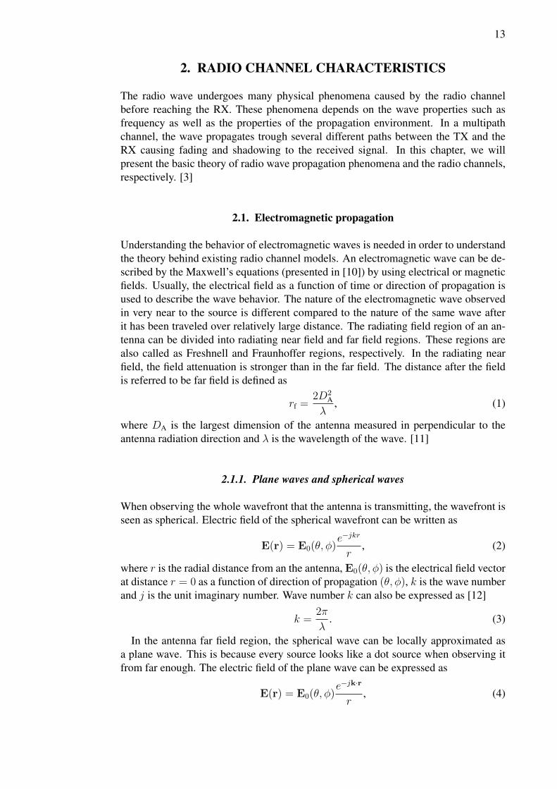
Understanding the behavior of electromagnetic waves is needed in order to understandthe theory behind existing radio channel models. An electromagnetic wave can be de-scribed by the Maxwell’s equations (presented in [10]) by using electrical or magneticfields. Usually, the electrical field as a function of time or direction of propagation isused to describe the wave behavior. The nature of the electromagnetic wave observedin very near to the source is different compared to the nature of the same wave afterit has been traveled over relatively large distance. The radiating field region of an an-tenna can be divided into radiating near field and far field regions. These regions arealso called as Freshnell and Fraunhoffer regions, respectively. In the radiating nearfield, the field attenuation is stronger than in the far field. The distance after the fieldis referred to be far field is defined as

rf =2D2

A

λ, (1)

where DA is the largest dimension of the antenna measured in perpendicular to theantenna radiation direction and λ is the wavelength of the wave. [11]

2.1.1. Plane waves and spherical waves

When observing the whole wavefront that the antenna is transmitting, the wavefront isseen as spherical. Electric field of the spherical wavefront can be written as

E(r) = E0(θ, φ)e−jkr

r, (2)

where r is the radial distance from an the antenna, E0(θ, φ) is the electrical field vectorat distance r = 0 as a function of direction of propagation (θ, φ), k is the wave numberand j is the unit imaginary number. Wave number k can also be expressed as [12]

k =2π

λ. (3)

In the antenna far field region, the spherical wave can be locally approximated asa plane wave. This is because every source looks like a dot source when observing itfrom far enough. The electric field of the plane wave can be expressed as

E(r) = E0(θ, φ)e−jk·r

r, (4)

14

where k is a complex wave vector and r is a position vector defining a point in 3D(Three Dimensional) space. [12]

2.1.2. Polarization

The polarization of the electromagnetic wave describes the time-varying direction andrelative magnitude of the electric-field vector. In the 3D vector-space, the polarizationdescribes the function of how the electric field vector varies among the direction ofpropagation (or ωt-axis). We can classify different kind of polarizations to be linear,circular and elliptical. When the electric field is oscillated only in one line, the wavecan be said to be linearly polarized. Linear polarization can always be reduced to twopolarization components; vertical and horizontal. In vertical polarization, the electricalfield is oscillating vertically among the y-axis with respect to the direction of propaga-tion (time-axis). In horizontal polarization, the same happens in the horizontal plane,i.e the electrical field is oscillating among the x-axis. In circular polarization, the elec-tric field goes around the circular orbit over the time-axis with a constant amplitude.In elliptical polarization, the electrical field vector goes around the elliptical orbit overthe time-axis and the amplitude is also varying. In case of elliptically polarized wave,we can define the axial ratio of an ellipse that the electrical field vector is tracing. Theaxial ratio is the ratio of the magnitudes of the major axis and minor axis. In case ofcircular polarization, the axial ratio is one. [13]

The polarization of an antenna is said to be same as the polarization of the radiowave the antenna is radiated. Therefore, vertically polarized antenna receives poorlyhorizontal polarized waves. Same goes the other way around. However, in the radiochannel, the polarization is not always the same in the TX and the RX. Thus, thepolarization can change while the wave is traveling trough the radio channel due to thedifferent propagation phenomena presented in next Sections. [13]

The polarization vector ρp represents the polarization of the wave. The polarizationvector is simply the unit vector pointing to the direction of the electric field. [13]

2.2. Propagation in the radio channel

By radio channel we mean the whole radio system including the TX, the RX andthe propagation channel. Depending on the channel geometry and the propagationmaterials, the radio wave may travel trough several different paths between the RX andTX. Thus, the radio wave undergoes several radio propagation phenomena between theTX and RX, which all affects to the wave behavior in the channel. In this section wewill present the basic radio propagation phenomena, which are valid especially forindoor propagation environment. [14]

2.2.1. Free space path loss

The propagation medium is defined to be free space, when the first Fresnel ellipsoid isclear from obstacles. In case of some obstacles within the Fresnel zone, the transmitted

15

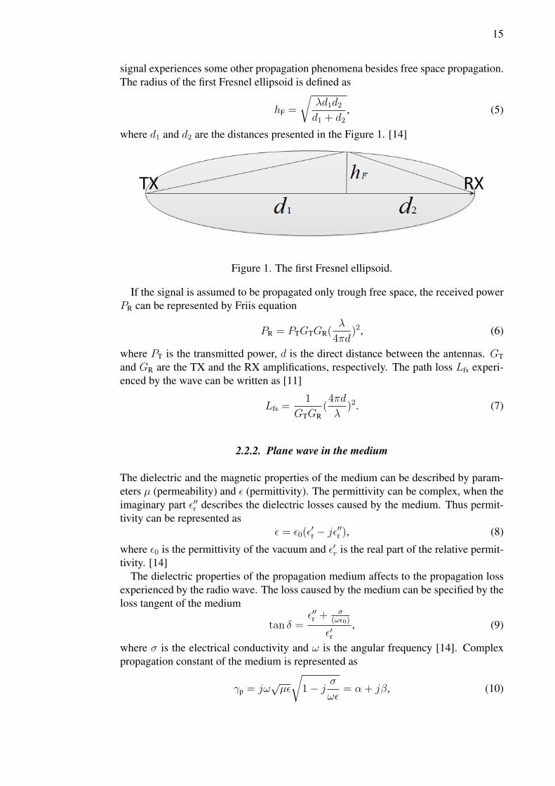
signal experiences some other propagation phenomena besides free space propagation.The radius of the first Fresnel ellipsoid is defined as

hF =

√λd1d2d1 + d2

, (5)

where d1 and d2 are the distances presented in the Figure 1. [14]

Figure 1. The first Fresnel ellipsoid.

If the signal is assumed to be propagated only trough free space, the received powerPR can be represented by Friis equation

PR = PTGTGR(λ

4πd)2, (6)

where PT is the transmitted power, d is the direct distance between the antennas. GT

and GR are the TX and the RX amplifications, respectively. The path loss Lfs experi-enced by the wave can be written as [11]

Lfs =1

GTGR(4πd

λ)2. (7)

2.2.2. Plane wave in the medium

The dielectric and the magnetic properties of the medium can be described by param-eters µ (permeability) and ε (permittivity). The permittivity can be complex, when theimaginary part ε′′r describes the dielectric losses caused by the medium. Thus permit-tivity can be represented as

ε = ε0(ε′r − jε′′r ), (8)

where ε0 is the permittivity of the vacuum and ε′r is the real part of the relative permit-tivity. [14]

The dielectric properties of the propagation medium affects to the propagation lossexperienced by the radio wave. The loss caused by the medium can be specified by theloss tangent of the medium

tan δ =ε′′r + σ

(ωε0)

ε′r, (9)

where σ is the electrical conductivity and ω is the angular frequency [14]. Complexpropagation constant of the medium is represented as

γp = jω√µε

√1− j σ

ωε= α + jβ, (10)

16

where α is the propagation coefficient and β is the phase coefficient. [15]The attenuation of the wave is exponential with respect to complex propagation con-

stant γp. The attenuation Lm(d) of the planar wave can be represented as

Lm(d) = eγpdm , (11)

where dm is the distance which the wave has been propagated in the medium. [14]

2.2.3. Plane wave in the media boundary

When a planar radio wave comes to the boundary of two different propagation media,some part of the wave power is reflected back form the boundary while the rest of thewave power propagates into the medium. Snell’s law for reflection is represented as

θr = θi, (12)

where θr is the angle of reflected wave and θi is the incident angle of the wave. [11]The polarization of the wave affects to the wave behavior at the media boundary.

The amount of relative power reflecting back form the boundary can be expressed bythe reflection coefficients specified for both perpendicular and parallel electric fieldcomponents with respect to the boundary. Hence, the polarization vector of the wavemay be changed due to the reflection, but not the actual polarization. This means that alinearly polarized wave stays linearly polarized also after the incidence. The reflectioncoefficients for the perpendicular and parallel polarizations can be expressed as [16]

R⊥ =cos θi −

√ε2ε1− sin2 θi√

ε2ε1− sin2 θi + cos θi

and R‖ =

√ε2ε1− sin2 θi − ε2

ε1cos θi√

ε2ε1− sin2 θi + ε2

ε1cos θi

. (13)

As part of the wave is reflected back from the media boundary, the rest of the energyis propagated trough the boundary inside the medium. The propagation angle of thewave may change depending on the relation of the dielectric properties of the media.Thus, the wave undergoes refraction in the media boundary. If we denote θt as theangle of the refracted wave, the propagation angle can be calculated by the Snell’s lawfor refraction

sin θt

sin θi=

√ε1√ε2

, (14)

where ε1 and ε2 are the permittivities of first and second propagation medium. [14]In case of orthogonal incidence, the transmission coefficients of the wave can be

expressed as [16] [14]

T⊥ = 1 +R⊥ and T‖ = 1 +R‖. (15)

If the incidence is not orthogonal, i.e θi 6= 90, the transmission coefficients can bewritten as

T⊥ =2 cos θi√

ε2ε1− sin2 θi + cos θi

and T‖ =2√

ε2ε1

cos θi√ε2ε1− sin2 θi + ε2

ε1cos θi

. (16)

17

2.2.4. Plane wave in rough surfaces and diffracting edges

In scattering, the small particles along the propagation path absorbs some energy andradiates it again to the around space, while acting as small antennas by themselves.When there are many of these particles along the propagation path, the scattering effectcan be significant and cause fading to the received signal. For example clouds andbushes are just an examples about obstacles causing scattering. Also rough surfaces,whose roughness is close to the wavelength, causes scattering. For the scattering, thereexist several models and theorems which are not presented here. Generally speaking,we can note that the effect of scattering to the radio wave is random and hence must bemodeled statistically. [16]

When some obstacle comes inside the first Fresnels zone, the wave is diffracted fromthe edge of the obstacle. If the obstacle is assumed to be wedge-shaped, it can be ap-proximated as a conducting half plane, i.e a knife edge. By the Huygens principle,every point of a radiating field can be referred to be the dot source of new electromag-netic field. geometrical optics (GO) defines the Snell’s law of diffraction as

n1 sin θi = n2 sin θd, (17)

where n1 and n2 are the refractive indices of the media 1 and 2, respectively and θd isthe diffraction angle of the wave. The Snell’s law for diffraction approximate wavesas rays (ray tubes), and it does not take into account the attenuation that the waveundergoes because of diffraction. [17]

If the knife-edge diffraction (KED) -approximation is used, we can also calculatetheoretical diffraction coefficient. The diffraction parameter ν can be expressed as

ν =√

2H

hF, (18)

where H denotes the height of the obstacle with respect to the direct link chord. TheKED-coefficient can be expressed as

F (ν) =1

2(1− (1− j)(C(ν)− jS(ν))), (19)

where C(ν) and S(ν) are Fresnel integrals defined as

C(ν) =

∫ ν

0

cos(π

2ξ2)dξ and S(ν) =

∫ ν

0

sin(π

2ξ2)dξ, (20)

where ξ is the auxiliary variable for the integral. [12] Diffraction loss factor is theabsolute value of the diffraction coefficient. To avoid the calculus of complex Fresnelintegrals, approximations can be used to calculate the diffraction coefficient for certainν-values. For ν > −0.7, the diffraction loss Lke in dBs can be approximated as [18]

Lke = 6.9 + 20 log(√

(ν − 0.1)2 + 1 + ν − 0.1). (21)

Instead of modeling the diffraction by wedges by KED, absorbing screen can also beused to model diffraction. For a plane wave incidence, the absorbing screen approach

18

gives us a geometrical theory of diffraction (GTD) diffraction coefficient with respectto θd as

Das(θd) =−√λ

2π

( 1

θd− 1

2π − θd

). (22)

The wavefront after diffraction is astigmatic because there is some caustic in the edge.GTD and uniform theory of diffraction (UTD) defines also other similar coefficientsfor the diffraction. As well as in the reflection and refraction, the polarization vectorof the wave may be changed due to the diffraction. [16] [12]

2.2.5. Fading and shadowing

Fading is defined as the deviation in radio channel causing attenuation to the transmit-ted wave. In a rich multipath channel, the transmitted wave propagates trough manydifferent propagation paths causing deviation to the received signal. All multipaths aresummed in the RX by the superposition principle. Fading can occur in time-, space-and frequency domain and it can be modeled statistically. Thus, fading is a randomprocess whose quantities depends on the propagation environment and mobility in thechannel. [3]

In Rician fading, Rice-distribution is used to describe the randomness of the channel.Rician fading is used, when one of the received multipath components are relativelystrong compared to others. Typical case of Rician fading is the LOS-environment. TheRician distribution is a function of two parameters, Kr and Ωr. The probability densityfunction (PDF) of the Rician distribution is defined as

f(x) =2(Kr + 1)x

Ωrexp(−Kr −

2(Kr + 1)x2

Ωr)I0(2

√2(Kr + 1)x

Ωr), (23)

where Kr is said to be a Rician K-factor defined as the ratio of the strongest multipath(typically LOS) compared to other multipaths, I0 is the Bessel function and Ωr is thetotal power of all the propagation paths. [19]

Rayleigh fading is typically used in NLOS-environment. In the Rayleigh fading,the magnitude of the received signal follows Rayleigh distribution described by theparameter Ωr. The PDF of Rayleigh distribution can be written as [19]

f(x) =2x

Ωrexp(−x

2

Ωr). (24)

2.3. Radio channel modeling

The radio channel models are usually defined to deterministic and stochastic channelmodels. Some of them are defined based on theory while others are based on the mea-surement data. The stochastic models relay on statistical distribution of the channel,while deterministic models tries to model the path loss in the channel deterministicallyby using for example the geometry of the propagation environment. In geometry baseddeterministic channel modeling ray tracing (RT) is often used. By the RT we mean the

19

geometry based radio wave path estimation between the TX and RX. In this section wepresent some key parameters and theory related to radio channel modeling.

2.3.1. Frequency and impulse responses

The channel frequency response is used to describe the channel behavior as a functionof frequency. When multiplying transmitted signal spectrum X(f) by the frequencyresponse H(f), we get the received signal spectrum Y (f). In frequency domain thiscan be expressed as [20]

Y (f) = H(f)X(f). (25)

In time domain, the channel is described by the channel impulse response h(t). Theimpulse response is the inverse Fourier transform of the frequency response, hence thereceived signal y(t) in time domain can be expressed as

y(t) = h(t) ∗ x(t), (26)

where x(t) is the transmitted signal and (∗) denotes the time domain convolution ofthe signals. [20]

In the radio channel modeling, the power of different signal paths is often interest-ing. Power delay profile (PDP ) of the channel is defined by the impulse responserepresenting the powers received at each time instant. It can be written as [3]

PDP (τ) = |h(t)|2. (27)

2.3.2. Delay spread, doppler spread and angular spread

There are few parameters to describe the properties of the multipath channel. Delayspread is a measure of the multipath richness of the propagation channel. It is definedby the PDP as being the time difference between the earliest and the latest significantmultipath component seen in the received signal PDP . In LOS-channel, the earliestcomponent is the LOS-propagated component of the signal. Mean delay spread androot mean square (RMS) -delay spread are parameters describing the deviation of thereceived signal path delays. The mean delay spread is defined as [3]

τ =

∫∞0τPDP (τ)dτ∫∞

0PDP (τ)dτ

, (28)

where τ is the delay at each multipath component. The RMS-delay spread is definedas [3]

τRMS =

√∫∞0

(τ − τ)2PDP (τ)dτ∫∞0PDP (τ)dτ

. (29)

The coherence bandwidth of the channel can be defined as the Fourier transform ofthe delay spread. The coherence bandwidth defines the bandwidth which the chan-nel stays constant with respect to frequency. Roughly, it can be approximated by theinverse of the mean delay spread [3]

BC ≈1

τ. (30)

20

If the TX, the RX or the environment is in motion over time, the transmitted signalexperiences Doppler effect. Thus, in the received spectrum (Doppler spectrum), sev-eral frequency components may be seen even if only one was transmitted. The spreadof the frequencies in the RX caused by the Doppler effect is called as Doppler spread.The width of the Doppler spectrum is called as Doppler bandwidth, BD [3] [17]. Chan-nel coherence time TC is inversely proportional to the Doppler bandwidth and it can bewritten as [3]

TC ≈1

BD. (31)

In a multipath channel, the multipath propagated components leaves from the TXantenna and arrives to RX antenna in some specific angle with respect to some refer-ence direction, which is usually the direct link path between the TX and RX. Theseangles are called as angle of departure (AoD) and angle of arrival (AoA), respectively.In three dimensional (3D) space, AoA and AoD is often defined separately for azimuthand elevation domains. Thus, the azimuth and elevation angles can be extended into3D as direction of arrival (DoA) and direction of departure (DoD). The Angular spreadis a parameter to describe the spatial order of the channel. [3]

2.3.3. Deterministic channel models

The deterministic channel models tries to estimate the path loss and phase differenceexperienced by the signal as it propagates trough the channel. The deterministic pathloss models, such as the free space path loss model presented in (7), are used to calcu-late the path loss of the channel. The models include a number of approximations andall of the radio propagation phenomena are not usually taken into account. This meansthat we have to simplify the geometry of the environment in order to estimate the mostsignificant multipaths from the impulse responses. The models are parameterized to fitto the propagation environment.

One deterministic channel model, the simplified path loss model, is defined as

L = Lref − 10γ log10[d

d0], (32)

where L is the path loss, γ is the path loss exponent, Lref is the path loss at the referencedistance d0 and d is the distance in meters. [3]

2.3.4. Indoor channel modeling

The indoor environment has many characteristics making them different from outdoorenvironment. At indoor environment, the walls are limiting the radio wave propagationespecially in higher frequencies, because of high wall penetration loss. On the otherhand, the walls gives a possibility to isolate the area better and hence avoid interfer-ence coming from outside or other rooms. The reflection, diffraction and free spacepropagation are the main propagation phenomena at the indoor environment if the pen-etration loss of the walls are assumed to be high. Long corridors makes it possible totransmit signals trough multiple reflections from the source to the destination. [3]

21

From the channel modeling and measurement point of view, indoor environment hastwo properties that makes the measurements easier. First, the environment can often bereferred to be static. Thus, the mobility in the channel is low (channel coherence timeis large). This is the case for example in the office environment. In some indoor en-vironments, such as shopping malls, there is often people moving in the environment,when the channel is static anymore. However, the mobility is still quite low comparedto the outdoor channels where we can have for example cars in the environment. Sec-ond, the distances that the channel models needs to support is usually smaller thanat the outdoor environment. This means that less dynamic range is required and thechannel can be assumed to be constant during the measurements.

2.3.5. MIMO channel modeling

To exploit the multipath channel to achieve the better system performance in a telecom-munication system, more than one antennas can be used in the TX and the RX ends. Inthat case, one pair between the RX and the TX antennas represents one single input sin-gle output (SISO) channel in the system. Thus MIMO system has several subchannelsthat can be combined to one MIMO-channel matrix. The matrix consists the subchan-nel coefficients from each TX antenna to all the RX antennas. If we denote hij beingthe channel coefficient from the TX antenna i to the RX antenna j, the MIMO-channelmatrix can be written as [3]

H =

h1,1 h1,2 · · · h1,nT

h2,1 h2,2 · · · h2,nT...

... . . . ...hnR,1 hnR,2 · · · hnR,nT

. (33)

In order to have an advantage on using multiple antennas, the channels must be asuncorrelated as possible. In case of correlated channel, the rank of the channel matrixis low. Furthermore, this means that the number of distinguishable multipaths in thechannel is low and hence MIMO cannot be successfully employed for beamforming.The best advantage of using multiple antennas is exceeded when the channel is as richas possible, meaning high rank of the channel matrix H.

Especially in the future telecommunication systems, the number of antennas areincreased in order to exploit better the multipath richness of the channel. If the TXand RX are equipped with very large number of antennas, the system is called massiveMIMO -systems. [1]

22

3. RADIO CHANNEL MEASUREMENT SETUP

When measuring the MIMO channel, the measurements with a good accuracy withrespect to the dynamic range of the system may take a significant amount of time. Inmassive MIMO systems where both ends contains hundreds of antennas, the increaseof amount of measurement time is multiplicative with respect the number of anten-nas. Furthermore, increasing the number of antennas increases the amount of recordedmeasurement data.

One key design principle of the designed measurement system was to do the systemas versatile as possible so that it could be applied to several channel measurements inthe future. We wanted to parameterize the software so that the system supports variousmeasurement options chosen by the user.

In this chapter, we introduce the measurement system for measuring the MIMOradio channel at 10 GHz. VNA based measurement setup with virtual planar antennaarrays in the RX and the TX ends is presented. The programming of the devices isintroduced, but the actual MATLAB implementations are not included to this thesis.However, some flow charts of the measurement control software are found from theAppendix.

3.1. VNA based measurement system

There are only few good ways to measure the radio propagation channel. When mea-suring a MIMO channel, channel sounders are usually a useful devices to be used.However, there are few drawbacks limiting the usage of the channel sounders. Firstdrawback is the prize of the apparatus. The commercial channel sounders are expen-sive and are not always easily available for high frequencies. Second drawback is thesynchronization of the RX- and TX clocks. Even though the high precision rubidiumclocks were used, there is still some imprecision in timing. The third problem is thelarge antenna arrays used for the measurements. For every frequency range measured,specified antenna array has to be designed individually.

Other good possibility is to use VNA with virtual antenna array. Now, only fewphysical antenna elements are used and the antenna is moved between positions torepresent an antenna array. One drawback is that the produced measurement resultdoes not take into account the correlation between antennas in the one end. On theother hand, simple measurement setup can be used with the device that can be lateron applied to the various applications. Furthermore, the system can be scaled to otherfrequencies simply by changing the VNA parameters and using different antennas. Ifthe VNA:s own frequency range is not enough, mixers can be used to increase VNAfrequency range. However, using external mixers may increase the system noise aswell.

One drawback in virtual antenna array based systems is the increased measurementtime. Antenna movement between the VNA sweeps increases the measurement timesignificantly. Also if narrow IF-bandwidth was used, one sweep would take hundredsof milliseconds of time. The trade of between the needed dynamic range and themeasurement speed is needed and the overall performance has to be optimized withrespect the desired property. [5]

23

3.1.1. The proposed measurement setup

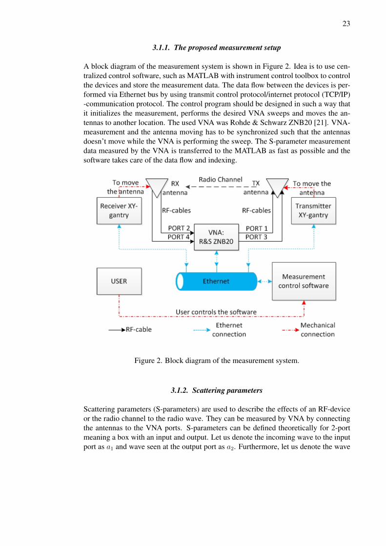
A block diagram of the measurement system is shown in Figure 2. Idea is to use cen-tralized control software, such as MATLAB with instrument control toolbox to controlthe devices and store the measurement data. The data flow between the devices is per-formed via Ethernet bus by using transmit control protocol/internet protocol (TCP/IP)-communication protocol. The control program should be designed in such a way thatit initializes the measurement, performs the desired VNA sweeps and moves the an-tennas to another location. The used VNA was Rohde & Schwarz ZNB20 [21]. VNA-measurement and the antenna moving has to be synchronized such that the antennasdoesn’t move while the VNA is performing the sweep. The S-parameter measurementdata measured by the VNA is transferred to the MATLAB as fast as possible and thesoftware takes care of the data flow and indexing.

Figure 2. Block diagram of the measurement system.

3.1.2. Scattering parameters

Scattering parameters (S-parameters) are used to describe the effects of an RF-deviceor the radio channel to the radio wave. They can be measured by VNA by connectingthe antennas to the VNA ports. S-parameters can be defined theoretically for 2-portmeaning a box with an input and output. Let us denote the incoming wave to the inputport as a1 and wave seen at the output port as a2. Furthermore, let us denote the wave

24

reflecting back towards the input and output ports as b1 and b2, respectively. For theS-parameters, we can write

S11 =b1a1

and S21 =a2a1

. (34)

Similar coefficients than (34) can be defined for wave coming to the output port. S21

can be referred to be the transmission coefficient of the 2-port and S11 as the reflectioncoefficient of the input port. S-parameters can be expanded for n-port as they weredefined for 2-port. [11]

3.1.3. VNA time domain analysis

S-parameters are usually presented in the frequency domain. The transition from fre-quency domain to time-domain can be done via inverse Fourier transform. There aretwo possibilities to get impulse responses out from the VNA. Many analyzers allowto measure the impulse responses directly in time domain, which are also called astime domain S-parameters by VNA vendors. However, we decided to measure theparameters in frequency domain and transform them into time domain via inverse dis-crete Fourier transform (IDFT). Let us denote Slm(fn) as the frequency domain S-parameters, where l and m are the port indices and fn is the n:th recorded frequencysample. By the IDFT, impulse responses hlm can be written as

hlm(tn) =1

Npoints

Npoints−1∑k=0

Slm(fk)ei2πkn/Npoints , (35)

where tn is the n:th time instant and Npoints is the number of frequency points [22].The measured bandwidth in frequency domain determines the time resolution in

time domain. Inverse fast fourier transform (IFFT) algorithm is used to calculate theIDFT. When using direct IFFT for the frequency domain samples measured by VNA,we obtain a time resolution of

δt =1

Bmeas, (36)

where Bmeas is the measured bandwidth. In time domain, the number of points, Npoints,is the same as in frequency domain, if zero padding is not performed while executingIFFT. Zero padding increases the resolution, but not accuracy because of interpolationand thus it should not be used in case of measured data. Thus, the length of the impulseresponse is written as [23]

∆t = (Npoints − 1)δt. (37)

The distance resolution of the recorded impulse responses can roughly be calculatedas

δd = δtc0, (38)

where c0 denotes the light speed in the free space. The length of the impulse responsein distance domain, i.e the maximum detectable path can be written as

∆d = ∆tc0 = (Npoints − 1)δd. (39)

25

3.2. Dynamic range of the measurement system

For each measurement, one should ensure that the dynamic range offered by the mea-surement system is reasonable for performing successful radio channel measurements.The dynamic range of the channel measurement system is defined as the differencebetween the highest and the lowest attenuations that the system is able to measure.When observing the lower limit, one should avoid the RF-components to drive intocompression. On the other hand, the attenuation caused by the channel should be lessthan the maximum attenuation supported by the system in order to be able to distinctthe actual signal from the noise. [5]

3.2.1. Noise in the measurement system

In reality, there is always some noise caused by the device in the radio system. Thereare different kind of noise sources in RF-electronics. The most significant one in radiofrequencies is the thermal noise caused by the resistive components. The thermal noiseis white, meaning that it remains constant over frequency. The power of the thermalnoise depends on the bandwidth B and the physical temperature T and can be writtenas

PN = kBTB, (40)

where kB is the Bolzmanns constant. It is usually assumed that T = T0 which is thesame as the nominal room temperature. [11]

Signal-to-noise ratio (SNR) is used to describe the signal versus noise quantity. Itis defined as

SNR =PS

PN, (41)

where PS and PN are the signal and noise powers, respectively. [14]

3.2.2. Noise factor, noise figure and noise temperature

For the radio devices, such as RX, we can define parameters to describe how muchnoise is appended to the system by the specific device. In an RF-amplifier, both thesignal and the noise are amplified to the output. The noise factor can be defined as

FN =SNRin

SNRout, (42)

where SNRin and SNRout are the signal-to-noise ratios at the input and output. Thenoise figure is the noise factor expressed in decibels and it can be written as [11]

NF = 10 log10 FN. (43)

Noise equivalent temperature Te describes the thermal noise existed in a radio block.For a radio component, it can be defied as

Te =N0

GkB, (44)

26

whereN0 is the noise power delivered to the output andG is the gain of the component.The relation of the noise temperature to the noise factor is [11]

Te = (F − 1)T0. (45)

3.2.3. Noise in cascaded radio blocks

The radio device consists many different kind of blocks in a chain which all affectsto the noise of the whole system. In a chain of RF-blocks connected in cascade, theoverall noise temperature can be calculated as [11]

Tcas = Te1 +

Nblocks∑i=2

Tei∏i−1j=1Gj

, (46)

where Nblocks is the number of blocks connected in cascade. Similarly, the overallnoise factor of the cascaded chain can be defined as

Fcas = F1 +

Nblocks∑i=2

Fi − 1∏i−1j=1Gj

. (47)

3.2.4. Noise in the VNA

Noise power in the VNA is proportional to its RX bandwidth as it was shown in Section3.2.1. The bandwidth B is limited by the IF-bandwidth of the RX. From the Equation(40) we see that doubling the bandwidth doubles also the noise power. [5]

Because the VNA has its own RX, it also has its own low noise amplifier LNA andits own RX noise figure NFVNA. Thus, the VNA:s own noise figure affects to the noisepower in the VNA. As it can be seen from the Equation (40), the thermal noise in thesystem is proportional to the bandwidth, but not to the actual frequency. The sensitivityof the VNA, i.e the smallest signal that the device can detect is limited by the noisefloor of the VNA. [5]

When using VNA, there are basically two ways to increase the dynamic range ofthe measurement system after all the input power available from VNA is used. Wecan make multiple sweeps and use averaging, or we can use narrower IF-bandwidthas shown in the Section 3.2.4. Both methods increases the measurement time signif-icantly. It is often said that the effect to the measurement time and dynamic range isroughly the same no matter which method was used. [5] However, when using averag-ing, we consider many channel realizations and thus measure the statistical propertiesof the channel. If the channel is assumed to be fixed during the measurements, it is bet-ter to use narrower IF-bandwidth to increase the dynamic range. By using this method,we loose the statistics, but we will have less measurement data to handle. [5]

3.2.5. Link budget and external amplifiers

In case of long link distances, the system requires also long cables to connect theantennas to the VNA ports. The signal attenuation in cables may grow significantly

27

large and hence reduce the dynamic range of the measurement system. As mentionedbefore, increasing the dynamic range of the system by averaging several sweeps orusing narrower IF-bandwidth in the VNA increases also the measurement time. Thus,using external amplifiers may be necessary to compensate the cable loss and keep thereceived signal above the RX sensitivity. [5]

Using external amplifiers causes two problems. As mentioned in the Section 3.2.3,the additional components in the RX chain increases the noise of the measurementsystem. Especially using external LNA in the RX front end increases the RX noise byits noise figure NFLNA. The overall noise factor (noise figure) can be calculated byusing Equation (47). Also the received signal should always be above the LNA:s ownnoise, i.e the sensitivity of the LNA should be adequate for the smallest received signallevel. If the external LNA is used, it has to have better noise figure than the VNA:sown RX in order to increase the sensitivity of the whole system. Thus, the sensitivityis not improved directly by the amplification of the LNA. If the LNA is placed directlyafter the RX antenna to compensate the long RF-cable, it is useful.

The second problem is how to include the amplifiers into the measurement calibra-tions in such a way that they will not damage the devices during the calibrations. Thecalibration problem can, however, be overcame by adding the amplifiers to the RF-chain after the calibrations and canceling them out from the measurements afterwards.If VNA would support the external amplifier selection by adding it to the rear panelof the VNA, we could also use that option to compensate the amplifier off from theresults. However, our VNA did not support this option. When using amplifiers, wealso need to ensure that the received power does not reach the level that drives the RXinto compression. Using external amplifiers does not necessarily increase the systemdynamic range, but shifts it down in the power region.

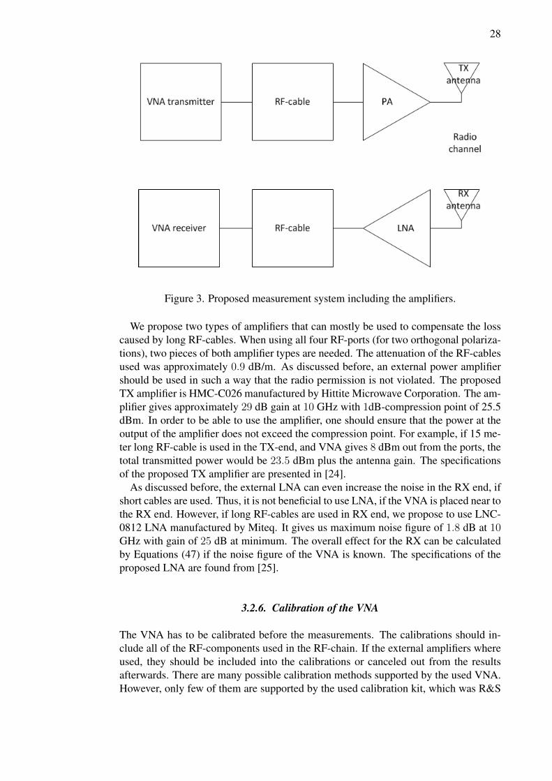
The measurement system should be able to be modified in such a way that the dy-namic range must be able to be scalded if needed in order to achieve good speed withrespect of accuracy. The external amplifiers were added to the measurement chainonly if the VNA:s own sensitivity was not enough. This is the case when the longRF-cables are used causing external attenuation to the signal, hence, decreasing thedynamic range left for the channel measurements. External LNA could be placed rightafter the RX antenna to increase the RX sensitivity. Power amplifier could be placedright before the TX antenna to increase the transmit power. If the measurement envi-ronment requires to use long cables (long links are wanted to be measured) the bestoption is to use long cables in both ends. However, this would require that the VNAshould most probably be placed between the antennas inside the measurement environ-ment affecting to the radio channel that is to be measured. Furthermore, the usage ofthe TX-amplifier is limited by the maximum power that is allowed to be used accord-ing to the radio permission. Also, the power performance of the VNA must be takeninto account such that the overall transmit power does not violate the radio permission.The idea is to first maximize the transmitted power and then minimize the RX noise.The RF-block chart of the measurement system including the external amplifiers ispresented in Figure 3.

28

Figure 3. Proposed measurement system including the amplifiers.

We propose two types of amplifiers that can mostly be used to compensate the losscaused by long RF-cables. When using all four RF-ports (for two orthogonal polariza-tions), two pieces of both amplifier types are needed. The attenuation of the RF-cablesused was approximately 0.9 dB/m. As discussed before, an external power amplifiershould be used in such a way that the radio permission is not violated. The proposedTX amplifier is HMC-C026 manufactured by Hittite Microwave Corporation. The am-plifier gives approximately 29 dB gain at 10 GHz with 1dB-compression point of 25.5dBm. In order to be able to use the amplifier, one should ensure that the power at theoutput of the amplifier does not exceed the compression point. For example, if 15 me-ter long RF-cable is used in the TX-end, and VNA gives 8 dBm out from the ports, thetotal transmitted power would be 23.5 dBm plus the antenna gain. The specificationsof the proposed TX amplifier are presented in [24].

As discussed before, the external LNA can even increase the noise in the RX end, ifshort cables are used. Thus, it is not beneficial to use LNA, if the VNA is placed near tothe RX end. However, if long RF-cables are used in RX end, we propose to use LNC-0812 LNA manufactured by Miteq. It gives us maximum noise figure of 1.8 dB at 10GHz with gain of 25 dB at minimum. The overall effect for the RX can be calculatedby Equations (47) if the noise figure of the VNA is known. The specifications of theproposed LNA are found from [25].

3.2.6. Calibration of the VNA

The VNA has to be calibrated before the measurements. The calibrations should in-clude all of the RF-components used in the RF-chain. If the external amplifiers whereused, they should be included into the calibrations or canceled out from the resultsafterwards. There are many possible calibration methods supported by the used VNA.However, only few of them are supported by the used calibration kit, which was R&S

29

ZV-Z5x [26]. VNA usually measures all of the S-parameters even though only fewof them are selected to be saved into defined traces. The ones not saved into traces,are dummy measurements, which only increases the measurement time. This meansthat we can speed up the measurement by calibrating the VNA only for the parameterswhich are supposed to be measured.

Each VNA vendor has their own calibration algorithms. For the radio channel mea-surements, the best calibration method offered by the used device is one way troughcalibration. However, this option was not supported by the used calibration kit andthus was not able to be used. Unknown trough open short match (UOSM) calibrationwere used instead. [27]

3.3. Virtual antenna array

When measuring the radio channel with the VNA, the number of VNA ports is limitingthe number of simultaneous antennas that could be used. To get still a MIMO channel,we move the antennas between the sweeps to get a virtual antenna array. The amountof movement between the measurement points depends on the antenna spacing of theused antenna array. Because of the channel correlation, usually antenna spacing of halfof the wavelength is used. [13]

There are several ways to perform the antenna movement between the measure-ment point. Especially in high frequencies such as 10 GHz, the misplacement of theantennas may cause significant inaccuracy to the measurements. When measuringlarge antenna configurations, the best way is to move antennas automatically by usingrobotics. Programmable devices such as robotic arms, or stepper motors can be usedfor the movement.

We built two XY-gantries to move the TX and the RX antennas to the vertical andthe horizontal directions by using programmable stepper motors. The motors wherechosen such that they could be controlled trough MATLAB along with the VNA.

3.3.1. Antenna characteristics

To be able to distinguish the effect of the propagation channel itself from the measureddata, the effect of the antennas should be compensated off from the data. Since inreality, antennas are not ideal components, all of the power fed into the antenna is notnecessarily radiated into the space. The impedance of an antenna is matched into theimpedance of the signal source. Thus, the antenna impedance is wanted to be as closeas possible to 50 Ω over the wanted frequency bandwidth in order to radiate well. Thematching of the antenna can be specified by the reflection coefficient S11. [13]

Reflection efficiency of the antenna takes into account the mismatch between thetransmission line and the antenna. The reflection efficiency can be defined as [13]

er = (1− |S11|2). (48)

30

Radiation efficiency of the antenna takes into account the conduction and dielectriclosses of the antenna. The radiation efficiency can be defined as

ecd =Rr

RL +Rr, (49)

where RL and Rr are the loss and radiation resistances, respectively. [13] The total an-tenna efficiency takes into account the losses at the input terminals within the structureof the antenna. Thus, the total antenna efficiency can be written as [13]

e0 = erecd. (50)

Directivity of the antenna, D(θ, φ), is defined as the ratio of the radiation intensityin a given direction from the antenna to the radiation intensity averaged over all direc-tions. Gain of the antenna is closely related to the directivity. It is a measure that takesinto account the efficiency of the antenna as well as its directional capabilities. Thus,the gain can be written as [13]

G(θ, φ) = ecdD(θ, φ). (51)

By taking into account also the impedance mismatch of the antenna, the absolute gainof the antenna can be defined as [13]

Gabs(θ, φ) = erecdD(θ, φ). (52)

The impedance of the antenna is complex and can be written as [13]

ZA = RA + jXA = RL +Rr + jXA, (53)

where ZA is the antenna impedance,RA is the antenna resistance andXA is the antennareactance. [13]

The −10 dB bandwidth of the antenna is defined as the frequency range where S11

is less than −10 dB. Polarization of the antenna in a given direction is defined as thepolarization of the wave transmitted (radiated) by the antenna. The polarization of theradio wave was defined in Section 2.1.2. The polarization loss factor (PLF ) describesthe polarization mismatch between the antenna and the wave. It can be written as

PLF = ρpA · ρpw, (54)

where ρpA and ρpW are the polarization vectors of the antenna and the wave, respec-tively. [13]

3.3.2. Dual polarized patch antenna

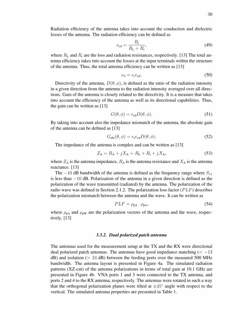
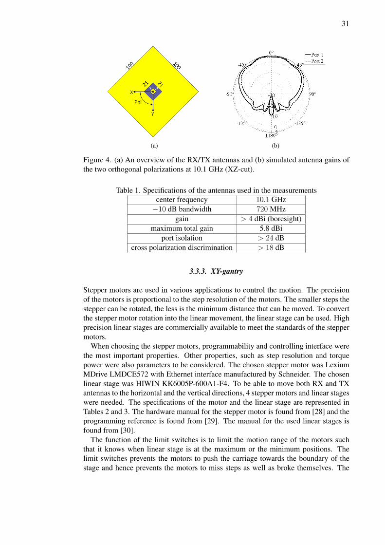
The antennas used for the measurement setup at the TX and the RX were directionaldual polarized patch antennas. The antennas have good impedance matching (< −13dB) and isolation (> 24 dB) between the feeding ports over the measured 500 MHzbandwidth. The antenna layout is presented in Figure 4a. The simulated radiationpatterns (XZ-cut) of the antenna polarizations in terms of total gain at 10.1 GHz arepresented in Figure 4b. VNA ports 1 and 3 were connected to the TX antenna, andports 2 and 4 to the RX antenna, respectively. The antennas were rotated in such a waythat the orthogonal polarization planes were tilted at ±45 angle with respect to thevertical. The simulated antenna properties are presented in Table 1.

31

(a) (b)

Figure 4. (a) An overview of the RX/TX antennas and (b) simulated antenna gains ofthe two orthogonal polarizations at 10.1 GHz (XZ-cut).

Table 1. Specifications of the antennas used in the measurementscenter frequency 10.1 GHz−10 dB bandwidth 720 MHz

gain > 4 dBi (boresight)maximum total gain 5.8 dBi

port isolation > 24 dBcross polarization discrimination > 18 dB

3.3.3. XY-gantry

Stepper motors are used in various applications to control the motion. The precisionof the motors is proportional to the step resolution of the motors. The smaller steps thestepper can be rotated, the less is the minimum distance that can be moved. To convertthe stepper motor rotation into the linear movement, the linear stage can be used. Highprecision linear stages are commercially available to meet the standards of the steppermotors.

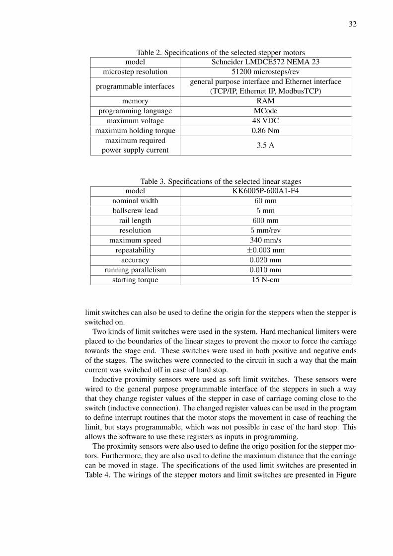
When choosing the stepper motors, programmability and controlling interface werethe most important properties. Other properties, such as step resolution and torquepower were also parameters to be considered. The chosen stepper motor was LexiumMDrive LMDCE572 with Ethernet interface manufactured by Schneider. The chosenlinear stage was HIWIN KK6005P-600A1-F4. To be able to move both RX and TXantennas to the horizontal and the vertical directions, 4 stepper motors and linear stageswere needed. The specifications of the motor and the linear stage are represented inTables 2 and 3. The hardware manual for the stepper motor is found from [28] and theprogramming reference is found from [29]. The manual for the used linear stages isfound from [30].

The function of the limit switches is to limit the motion range of the motors suchthat it knows when linear stage is at the maximum or the minimum positions. Thelimit switches prevents the motors to push the carriage towards the boundary of thestage and hence prevents the motors to miss steps as well as broke themselves. The

32

Table 2. Specifications of the selected stepper motorsmodel Schneider LMDCE572 NEMA 23

microstep resolution 51200 microsteps/rev

programmable interfacesgeneral purpose interface and Ethernet interface

(TCP/IP, Ethernet IP, ModbusTCP)memory RAM

programming language MCodemaximum voltage 48 VDC

maximum holding torque 0.86 Nmmaximum required

power supply current3.5 A

Table 3. Specifications of the selected linear stagesmodel KK6005P-600A1-F4

nominal width 60 mmballscrew lead 5 mm

rail length 600 mmresolution 5 mm/rev

maximum speed 340 mm/srepeatability ±0.003 mm

accuracy 0.020 mmrunning parallelism 0.010 mm

starting torque 15 N-cm

limit switches can also be used to define the origin for the steppers when the stepper isswitched on.

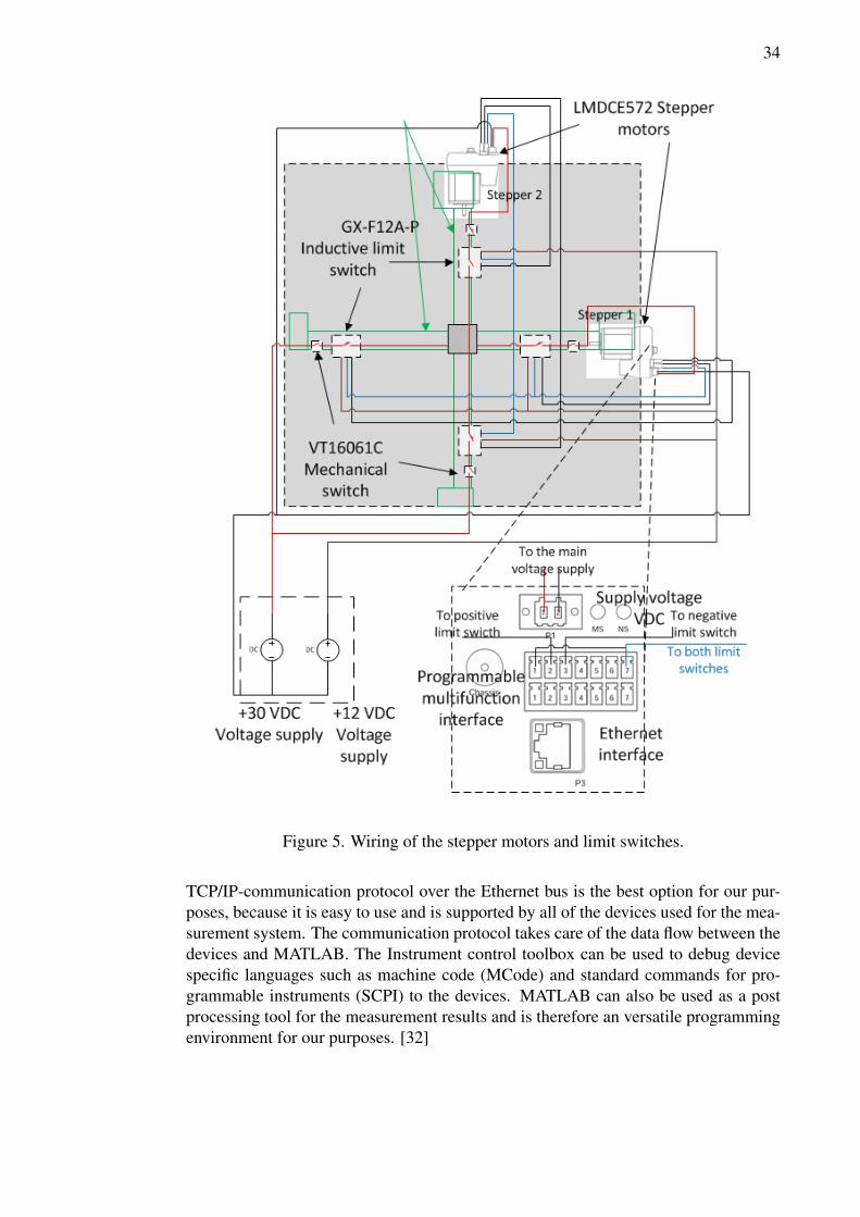
Two kinds of limit switches were used in the system. Hard mechanical limiters wereplaced to the boundaries of the linear stages to prevent the motor to force the carriagetowards the stage end. These switches were used in both positive and negative endsof the stages. The switches were connected to the circuit in such a way that the maincurrent was switched off in case of hard stop.

Inductive proximity sensors were used as soft limit switches. These sensors werewired to the general purpose programmable interface of the steppers in such a waythat they change register values of the stepper in case of carriage coming close to theswitch (inductive connection). The changed register values can be used in the programto define interrupt routines that the motor stops the movement in case of reaching thelimit, but stays programmable, which was not possible in case of the hard stop. Thisallows the software to use these registers as inputs in programming.

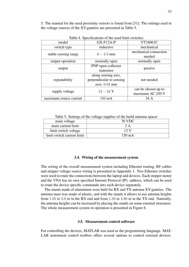
The proximity sensors were also used to define the origo position for the stepper mo-tors. Furthermore, they are also used to define the maximum distance that the carriagecan be moved in stage. The specifications of the used limit switches are presented inTable 4. The wirings of the stepper motors and limit switches are presented in Figure

33

5. The manual for the used proximity sensors is found from [31]. The settings used inthe voltage sources of the XY-gantries are presented in Table 5.

Table 4. Specifications of the used limit switchesmodel GX-F12A-P VT16061C

switch type inductive mechanical

stable sensing range 0− 3.3 mmmechanical connection

neededoutput operation normally open normally open

outputPNP open-collector

transistorpassive

repeatabilityalong sensing axis,

perpendicular to sensingaxis: 0.04 mm

not needed

supply voltage 12− 24 Vcan be chosen up tomaximum AC 250 V

maximum source current 100 mA 16 A

Table 5. Settings of the voltage supplies of the build antenna spacermain voltage 30 VDC

main current limit 2 Alimit switch voltage 12 V

limit switch current limit 150 mA

3.4. Wiring of the measurement system

The wiring of the overall measurement system including Ethernet routing, RF-cablesand stepper voltage source wiring is presented in Appendix 1. Two Ethernet switcheswere used to route the connections between the laptop and devices. Each stepper motorand the VNA has its own specified Internet Protocol (IP) -address, which can be usedto route the device specific commands into each device separately.

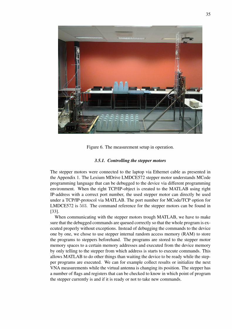
The stands made of aluminium were built for RX and TX antenna XY-gantries. Theantenna mast was made of plastic, and with the stands it allows to use antenna heightsfrom 1.05 to 2.0 m in the RX end and from 1.50 to 2.80 m in the TX end. Naturally,the antenna heights can be increased by placing the stands on some external structures.The whole measurement system in operation is presented in Figure 6.

3.5. Measurement control software

For controlling the devices, MATLAB was used as the programming language. MAT-LAB instrument control toolbox offers several options to control external devices.

34

Figure 5. Wiring of the stepper motors and limit switches.

TCP/IP-communication protocol over the Ethernet bus is the best option for our pur-poses, because it is easy to use and is supported by all of the devices used for the mea-surement system. The communication protocol takes care of the data flow between thedevices and MATLAB. The Instrument control toolbox can be used to debug devicespecific languages such as machine code (MCode) and standard commands for pro-grammable instruments (SCPI) to the devices. MATLAB can also be used as a postprocessing tool for the measurement results and is therefore an versatile programmingenvironment for our purposes. [32]

35

Figure 6. The measurement setup in operation.

3.5.1. Controlling the stepper motors

The stepper motors were connected to the laptop via Ethernet cable as presented inthe Appendix 1. The Lexium MDrive LMDCE572 stepper motor understands MCodeprogramming language that can be debugged to the device via different programmingenvironment. When the right TCP/IP-object is created to the MATLAB using rightIP-address with a correct port number, the used stepper motor can directly be usedunder a TCP/IP-protocol via MATLAB. The port number for MCode/TCP option forLMDCE572 is 503. The command reference for the stepper motors can be found in[33].

When communicating with the stepper motors trough MATLAB, we have to makesure that the debugged commands are queued correctly so that the whole program is ex-ecuted properly without exceptions. Instead of debugging the commands to the deviceone by one, we chose to use stepper internal random access memory (RAM) to storethe programs to steppers beforehand. The programs are stored to the stepper motormemory spaces to a certain memory addresses and executed from the device memoryby only telling to the stepper from which address is starts to execute commands. Thisallows MATLAB to do other things than waiting the device to be ready while the step-per programs are executed. We can for example collect results or initialize the nextVNA measurements while the virtual antenna is changing its position. The stepper hasa number of flags and registers that can be checked to know in which point of programthe stepper currently is and if it is ready or not to take new commands.

36

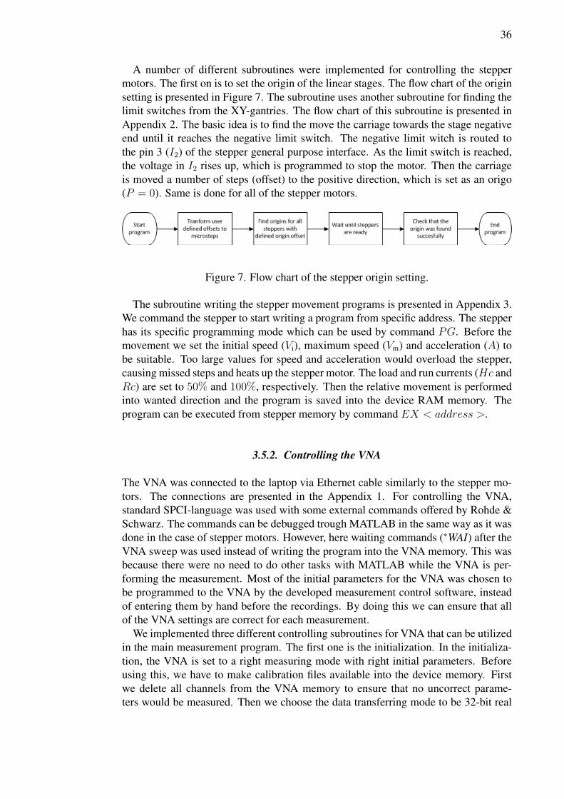
A number of different subroutines were implemented for controlling the steppermotors. The first on is to set the origin of the linear stages. The flow chart of the originsetting is presented in Figure 7. The subroutine uses another subroutine for finding thelimit switches from the XY-gantries. The flow chart of this subroutine is presented inAppendix 2. The basic idea is to find the move the carriage towards the stage negativeend until it reaches the negative limit switch. The negative limit witch is routed tothe pin 3 (I2) of the stepper general purpose interface. As the limit switch is reached,the voltage in I2 rises up, which is programmed to stop the motor. Then the carriageis moved a number of steps (offset) to the positive direction, which is set as an origo(P = 0). Same is done for all of the stepper motors.

Figure 7. Flow chart of the stepper origin setting.

The subroutine writing the stepper movement programs is presented in Appendix 3.We command the stepper to start writing a program from specific address. The stepperhas its specific programming mode which can be used by command PG. Before themovement we set the initial speed (Vi), maximum speed (Vm) and acceleration (A) tobe suitable. Too large values for speed and acceleration would overload the stepper,causing missed steps and heats up the stepper motor. The load and run currents (Hc andRc) are set to 50% and 100%, respectively. Then the relative movement is performedinto wanted direction and the program is saved into the device RAM memory. Theprogram can be executed from stepper memory by command EX < address >.

3.5.2. Controlling the VNA

The VNA was connected to the laptop via Ethernet cable similarly to the stepper mo-tors. The connections are presented in the Appendix 1. For controlling the VNA,standard SPCI-language was used with some external commands offered by Rohde &Schwarz. The commands can be debugged trough MATLAB in the same way as it wasdone in the case of stepper motors. However, here waiting commands (∗WAI) after theVNA sweep was used instead of writing the program into the VNA memory. This wasbecause there were no need to do other tasks with MATLAB while the VNA is per-forming the measurement. Most of the initial parameters for the VNA was chosen tobe programmed to the VNA by the developed measurement control software, insteadof entering them by hand before the recordings. By doing this we can ensure that allof the VNA settings are correct for each measurement.

We implemented three different controlling subroutines for VNA that can be utilizedin the main measurement program. The first one is the initialization. In the initializa-tion, the VNA is set to a right measuring mode with right initial parameters. Beforeusing this, we have to make calibration files available into the device memory. Firstwe delete all channels from the VNA memory to ensure that no uncorrect parame-ters would be measured. Then we choose the data transferring mode to be 32-bit real

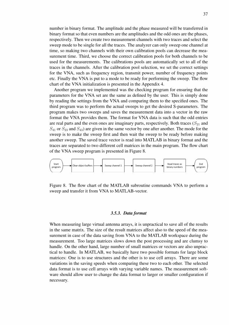
37

number in binary format. The amplitude and the phase measured will be transferred inbinary format so that even numbers are the amplitudes and the odd ones are the phases,respectively. Then we create two measurement channels with two traces and select thesweep mode to be single for all the traces. The analyzer can only sweep one channel attime, so making two channels with their own calibration pools can decrease the mea-surement time. Third, we choose the correct calibration pools for both channels to beused for the measurements. The calibrations pools are automatically set to all of thetraces in the channels. After the calibration pool selection, we set the correct settingsfor the VNA, such as frequency region, transmit power, number of frequency pointsetc. Finally the VNA is put to a mode to be ready for performing the sweep. The flowchart of the VNA initialization is presented in the Appendix 4.

Another program we implemented was the checking program for ensuring that theparameters for the VNA set are the same as defined by the user. This is simply doneby reading the settings from the VNA and comparing them to the specified ones. Thethird program was to perform the actual sweeps to get the desired S-parameters. Theprogram makes two sweeps and saves the measurement data into a vector in the rawformat the VNA provides them. The format for VNA data is such that the odd entriesare real parts and the even ones are imaginary parts, respectively. Both traces (S21 andS41 or S23 and S43) are given in the same vector by one after another. The mode for thesweep is to make the sweep first and then wait the sweep to be ready before makinganother sweep. The saved trace vector is read into MATLAB in binary format and thetraces are separated to two different cell matrices in the main program. The flow chartof the VNA sweep program is presented in Figure 8.

Figure 8. The flow chart of the MATLAB subroutine commands VNA to perform asweep and transfer it from VNA to MATLAB-vector.

3.5.3. Data format

When measuring large virtual antenna arrays, it is unpractical to save all of the resultsin the same matrix. The size of the result matrices affect also to the speed of the mea-surement in case of the data saving from VNA to the MATLAB workspace during themeasurement. Too large matrices slows down the post processing and are clumsy tohandle. On the other hand, large number of small matrices or vectors are also unprac-tical to handle. In MATLAB, we basically have two possible formats for large blockmatrices: One is to use structures and the other is to use cell arrays. There are somevariations in the saving speeds when comparing these two to each other. The selecteddata format is to use cell arrays with varying variable names. The measurement soft-ware should allow user to change the data format to larger or smaller configuration ifnecessary.

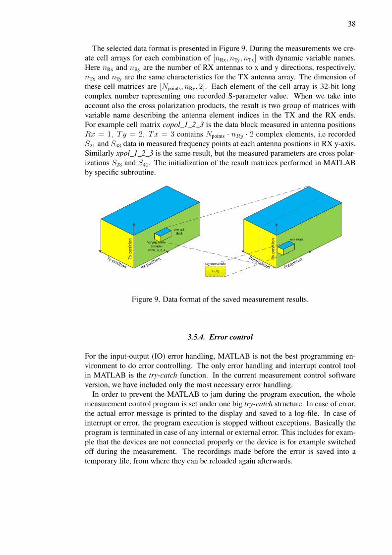
38

The selected data format is presented in Figure 9. During the measurements we cre-ate cell arrays for each combination of [nRx, nTy, nTx] with dynamic variable names.Here nRx and nRy are the number of RX antennas to x and y directions, respectively.nTx and nTy are the same characteristics for the TX antenna array. The dimension ofthese cell matrices are [Npoints, nRy, 2]. Each element of the cell array is 32-bit longcomplex number representing one recorded S-parameter value. When we take intoaccount also the cross polarization products, the result is two group of matrices withvariable name describing the antenna element indices in the TX and the RX ends.For example cell matrix copol_1_2_3 is the data block measured in antenna positionsRx = 1, T y = 2, Tx = 3 contains Npoints · nRy · 2 complex elements, i.e recordedS21 and S43 data in measured frequency points at each antenna positions in RX y-axis.Similarly xpol_1_2_3 is the same result, but the measured parameters are cross polar-izations S23 and S41. The initialization of the result matrices performed in MATLABby specific subroutine.

Figure 9. Data format of the saved measurement results.

3.5.4. Error control

For the input-output (IO) error handling, MATLAB is not the best programming en-vironment to do error controlling. The only error handling and interrupt control toolin MATLAB is the try-catch function. In the current measurement control softwareversion, we have included only the most necessary error handling.

In order to prevent the MATLAB to jam during the program execution, the wholemeasurement control program is set under one big try-catch structure. In case of error,the actual error message is printed to the display and saved to a log-file. In case ofinterrupt or error, the program execution is stopped without exceptions. Basically theprogram is terminated in case of any internal or external error. This includes for exam-ple that the devices are not connected properly or the device is for example switchedoff during the measurement. The recordings made before the error is saved into atemporary file, from where they can be reloaded again afterwards.

39

3.5.5. User interface

The measurement software is developed in such a way that the user can parameterizethe configuration by modifying a single input file called ’inputs.m’. Before the mea-surements, the user should perform the calibration manually and save the calibrationpool into the memory of the VNA. User can make his own calibrations for the bothof the measurement channels to speed up the measurement. The name of the appliedcalibration file has to be specified in the measurement input file, and the software setsautomatically the defined calibration pools into the measurement channels. The inputparameters that the user can set are given in the Appendix 5.

The main script of the control software uses subroutines defined in Sections 3.5.1and 3.5.2 to control the devices. The inputs given by the user as defined in Section3.5.5, are used to parameterize the program. A waiting period is added in the verticaldirection movement because of vibrations of the antenna mast. The flow chart of themeasurement control software is presented in Appendix 6.

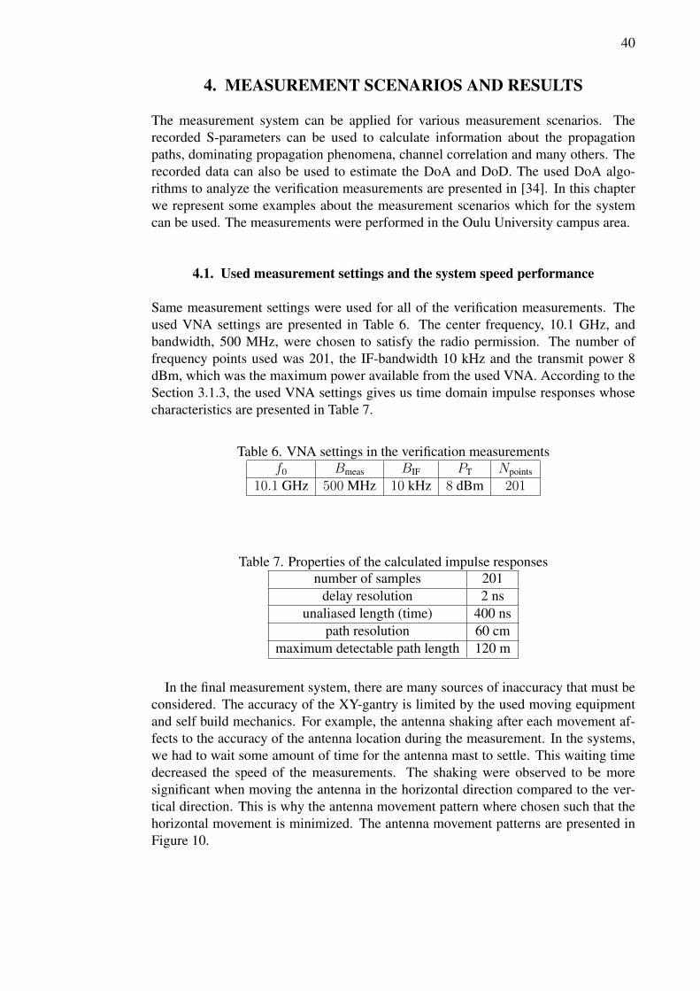
40

4. MEASUREMENT SCENARIOS AND RESULTS

The measurement system can be applied for various measurement scenarios. Therecorded S-parameters can be used to calculate information about the propagationpaths, dominating propagation phenomena, channel correlation and many others. Therecorded data can also be used to estimate the DoA and DoD. The used DoA algo-rithms to analyze the verification measurements are presented in [34]. In this chapterwe represent some examples about the measurement scenarios which for the systemcan be used. The measurements were performed in the Oulu University campus area.

4.1. Used measurement settings and the system speed performance

Same measurement settings were used for all of the verification measurements. Theused VNA settings are presented in Table 6. The center frequency, 10.1 GHz, andbandwidth, 500 MHz, were chosen to satisfy the radio permission. The number offrequency points used was 201, the IF-bandwidth 10 kHz and the transmit power 8dBm, which was the maximum power available from the used VNA. According to theSection 3.1.3, the used VNA settings gives us time domain impulse responses whosecharacteristics are presented in Table 7.

Table 6. VNA settings in the verification measurementsf0 Bmeas BIF PT Npoints

10.1 GHz 500 MHz 10 kHz 8 dBm 201

Table 7. Properties of the calculated impulse responsesnumber of samples 201

delay resolution 2 nsunaliased length (time) 400 ns

path resolution 60 cmmaximum detectable path length 120 m

In the final measurement system, there are many sources of inaccuracy that must beconsidered. The accuracy of the XY-gantry is limited by the used moving equipmentand self build mechanics. For example, the antenna shaking after each movement af-fects to the accuracy of the antenna location during the measurement. In the systems,we had to wait some amount of time for the antenna mast to settle. This waiting timedecreased the speed of the measurements. The shaking were observed to be moresignificant when moving the antenna in the horizontal direction compared to the ver-tical direction. This is why the antenna movement pattern where chosen such that thehorizontal movement is minimized. The antenna movement patterns are presented inFigure 10.

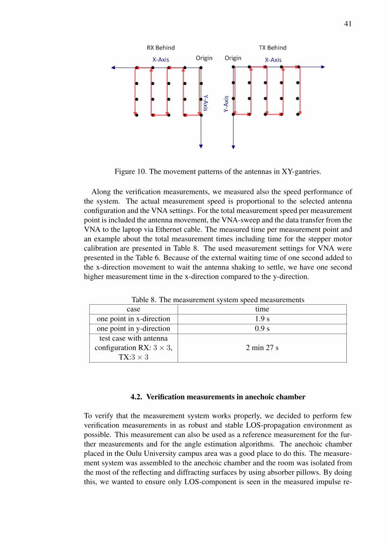
41

Figure 10. The movement patterns of the antennas in XY-gantries.

Along the verification measurements, we measured also the speed performance ofthe system. The actual measurement speed is proportional to the selected antennaconfiguration and the VNA settings. For the total measurement speed per measurementpoint is included the antenna movement, the VNA-sweep and the data transfer from theVNA to the laptop via Ethernet cable. The measured time per measurement point andan example about the total measurement times including time for the stepper motorcalibration are presented in Table 8. The used measurement settings for VNA werepresented in the Table 6. Because of the external waiting time of one second added tothe x-direction movement to wait the antenna shaking to settle, we have one secondhigher measurement time in the x-direction compared to the y-direction.

Table 8. The measurement system speed measurementscase time

one point in x-direction 1.9 sone point in y-direction 0.9 stest case with antenna

configuration RX: 3× 3,TX:3× 3

2 min 27 s

4.2. Verification measurements in anechoic chamber

To verify that the measurement system works properly, we decided to perform fewverification measurements in as robust and stable LOS-propagation environment aspossible. This measurement can also be used as a reference measurement for the fur-ther measurements and for the angle estimation algorithms. The anechoic chamberplaced in the Oulu University campus area was a good place to do this. The measure-ment system was assembled to the anechoic chamber and the room was isolated fromthe most of the reflecting and diffracting surfaces by using absorber pillows. By doingthis, we wanted to ensure only LOS-component is seen in the measured impulse re-

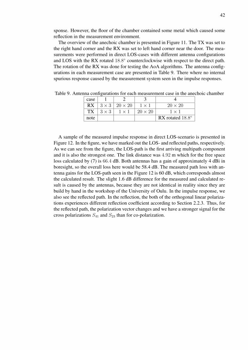
42

sponse. However, the floor of the chamber contained some metal which caused somereflection in the measurement environment.

The overview of the anechoic chamber is presented in Figure 11. The TX was set tothe right hand corner and the RX was set to left hand corner near the door. The mea-surements were performed in direct LOS-cases with different antenna configurationsand LOS with the RX rotated 18.8 counterclockwise with respect to the direct path.The rotation of the RX was done for testing the AoA algorithms. The antenna config-urations in each measurement case are presented in Table 9. There where no internalspurious response caused by the measurement system seen in the impulse responses.

Table 9. Antenna configurations for each measurement case in the anechoic chambercase 1 2 3 4RX 3× 3 20× 20 1× 1 20× 20TX 3× 3 1× 1 20× 20 1× 1note RX rotated 18.8

A sample of the measured impulse response in direct LOS-scenario is presented inFigure 12. In the figure, we have marked out the LOS- and reflected paths, respectively.As we can see from the figure, the LOS-path is the first arriving multipath componentand it is also the strongest one. The link distance was 4.92 m which for the free spaceloss calculated by (7) is 66.4 dB. Both antennas has a gain of approximately 4 dBi inboresight, so the overall loss here would be 58.4 dB. The measured path loss with an-tenna gains for the LOS-path seen in the Figure 12 is 60 dB, which corresponds almostthe calculated result. The slight 1.6 dB difference for the measured and calculated re-sult is caused by the antennas, because they are not identical in reality since they arebuild by hand in the workshop of the University of Oulu. In the impulse response, wealso see the reflected path. In the reflection, the both of the orthogonal linear polariza-tions experiences different reflection coefficient according to Section 2.2.3. Thus, forthe reflected path, the polarization vector changes and we have a stronger signal for thecross polarizations S41 and S23 than for co-polarization.

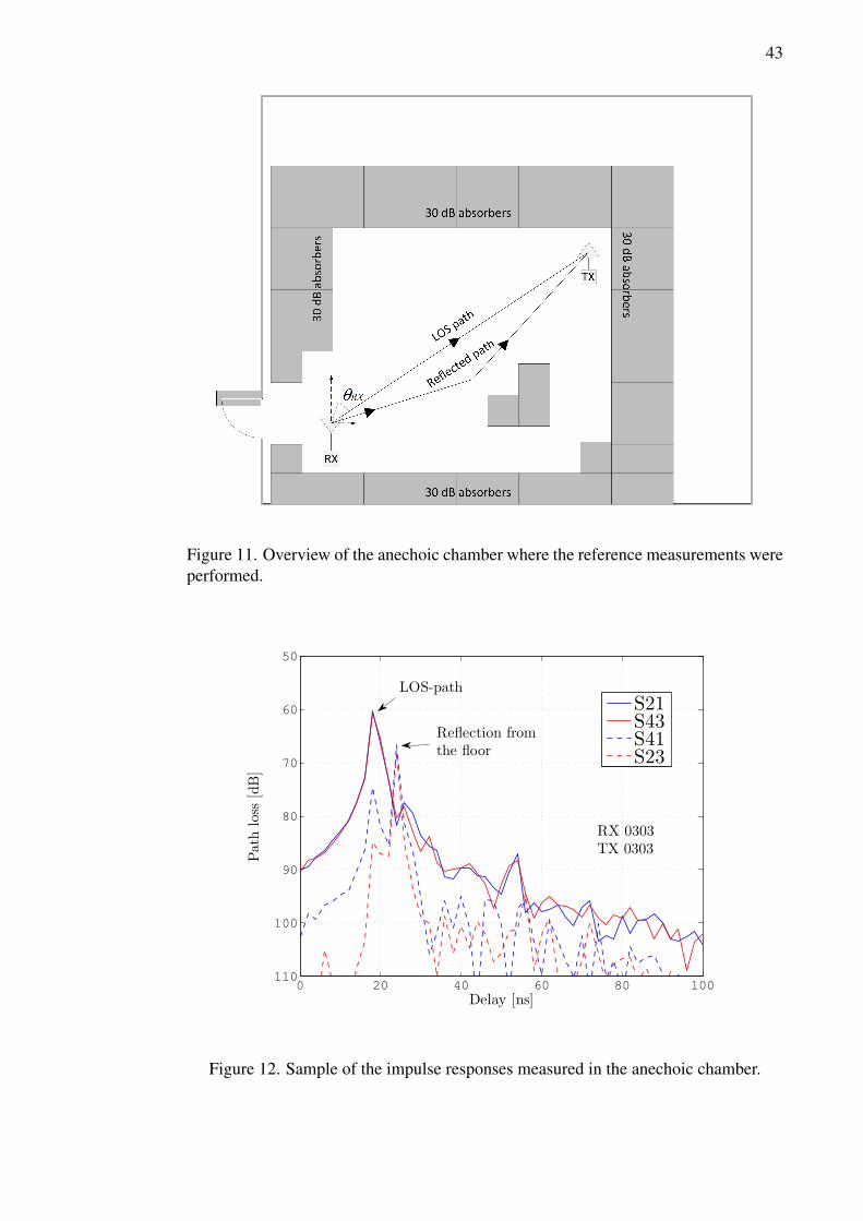
43

Figure 11. Overview of the anechoic chamber where the reference measurements wereperformed.

0 20 40 60 80 100−110

−100

−90

−80

−70

−60

−50

RX 0303TX 0303

Delay [ns]

Pathloss

[dB]

S21S43S41S23

LOS-path

Reflection fromthe floor

Figure 12. Sample of the impulse responses measured in the anechoic chamber.

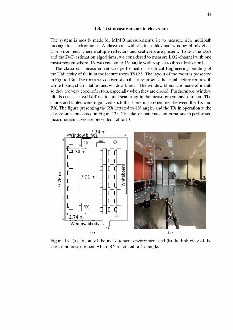
44

4.3. Test measurements in classroom

The system is mostly made for MIMO measurements, i.e to measure rich multipathpropagation environment. A classroom with chairs, tables and window blinds givesan environment where multiple reflectors and scatterers are present. To test the DoAand the DoD estimation algorithms, we considered to measure LOS-channel with onemeasurement where RX was rotated to 45 angle with respect to direct link chord.

The classroom measurement was performed in Electrical Engineering building ofthe University of Oulu in the lecture room TS128. The layout of the room is presentedin Figure 13a. The room was chosen such that it represents the usual lecture room withwhite board, chairs, tables and window blinds. The window blinds are made of metal,so they are very good reflectors, especially when they are closed. Furthermore, windowblinds causes as well diffraction and scattering in the measurement environment. Thechairs and tables were organized such that there is an open area between the TX andRX. The figure presenting the RX (rotated to 45 angle) and the TX in operation at theclassroom is presented in Figure 13b. The chosen antenna configurations in performedmeasurement cases are presented Table 10.

(a) (b)

Figure 13. (a) Layout of the measurement environment and (b) the link view of theclassroom measurement where RX is rotated to 45 angle.

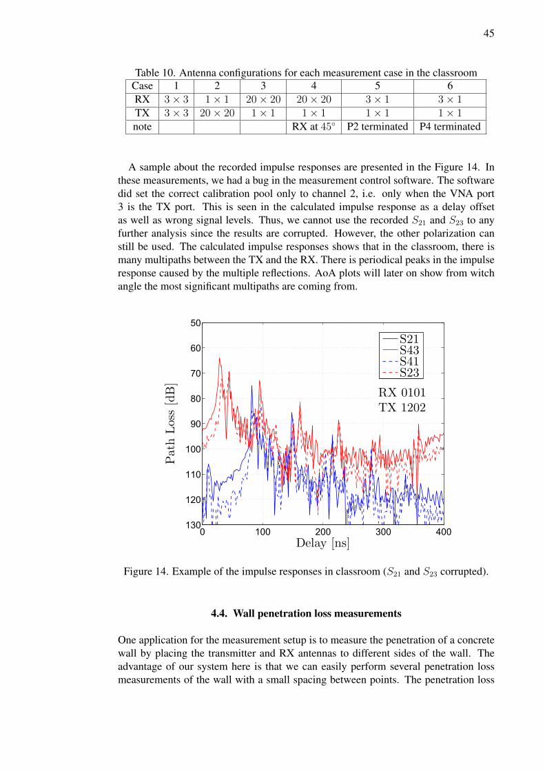
45

Table 10. Antenna configurations for each measurement case in the classroomCase 1 2 3 4 5 6RX 3× 3 1× 1 20× 20 20× 20 3× 1 3× 1TX 3× 3 20× 20 1× 1 1× 1 1× 1 1× 1note RX at 45 P2 terminated P4 terminated

A sample about the recorded impulse responses are presented in the Figure 14. Inthese measurements, we had a bug in the measurement control software. The softwaredid set the correct calibration pool only to channel 2, i.e. only when the VNA port3 is the TX port. This is seen in the calculated impulse response as a delay offsetas well as wrong signal levels. Thus, we cannot use the recorded S21 and S23 to anyfurther analysis since the results are corrupted. However, the other polarization canstill be used. The calculated impulse responses shows that in the classroom, there ismany multipaths between the TX and the RX. There is periodical peaks in the impulseresponse caused by the multiple reflections. AoA plots will later on show from witchangle the most significant multipaths are coming from.

0 100 200 300 400−130

−120

−110

−100

−90

−80

−70

−60

−50

RX 0101TX 1202

Delay [ns]

PathLoss

[dB]

S21S43S41S23

Figure 14. Example of the impulse responses in classroom (S21 and S23 corrupted).

4.4. Wall penetration loss measurements

One application for the measurement setup is to measure the penetration of a concretewall by placing the transmitter and RX antennas to different sides of the wall. Theadvantage of our system here is that we can easily perform several penetration lossmeasurements of the wall with a small spacing between points. The penetration loss

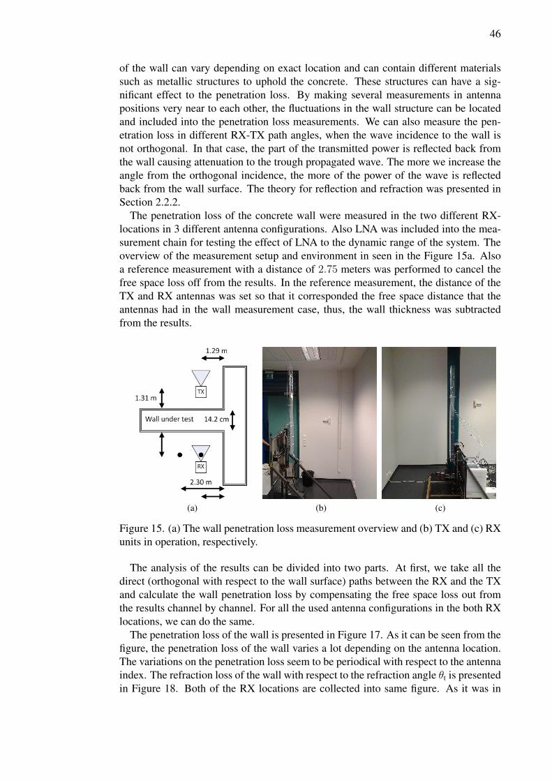
46

of the wall can vary depending on exact location and can contain different materialssuch as metallic structures to uphold the concrete. These structures can have a sig-nificant effect to the penetration loss. By making several measurements in antennapositions very near to each other, the fluctuations in the wall structure can be locatedand included into the penetration loss measurements. We can also measure the pen-etration loss in different RX-TX path angles, when the wave incidence to the wall isnot orthogonal. In that case, the part of the transmitted power is reflected back fromthe wall causing attenuation to the trough propagated wave. The more we increase theangle from the orthogonal incidence, the more of the power of the wave is reflectedback from the wall surface. The theory for reflection and refraction was presented inSection 2.2.2.

The penetration loss of the concrete wall were measured in the two different RX-locations in 3 different antenna configurations. Also LNA was included into the mea-surement chain for testing the effect of LNA to the dynamic range of the system. Theoverview of the measurement setup and environment in seen in the Figure 15a. Alsoa reference measurement with a distance of 2.75 meters was performed to cancel thefree space loss off from the results. In the reference measurement, the distance of theTX and RX antennas was set so that it corresponded the free space distance that theantennas had in the wall measurement case, thus, the wall thickness was subtractedfrom the results.

(a) (b) (c)

Figure 15. (a) The wall penetration loss measurement overview and (b) TX and (c) RXunits in operation, respectively.

The analysis of the results can be divided into two parts. At first, we take all thedirect (orthogonal with respect to the wall surface) paths between the RX and the TXand calculate the wall penetration loss by compensating the free space loss out fromthe results channel by channel. For all the used antenna configurations in the both RXlocations, we can do the same.

The penetration loss of the wall is presented in Figure 17. As it can be seen from thefigure, the penetration loss of the wall varies a lot depending on the antenna location.The variations on the penetration loss seem to be periodical with respect to the antennaindex. The refraction loss of the wall with respect to the refraction angle θt is presentedin Figure 18. Both of the RX locations are collected into same figure. As it was in

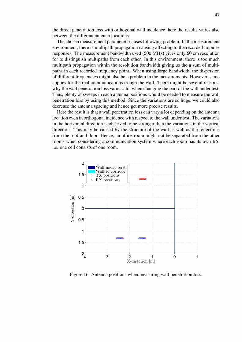
47

the direct penetration loss with orthogonal wall incidence, here the results varies alsobetween the different antenna locations.

The chosen measurement parameters causes following problem. In the measurementenvironment, there is multipath propagation causing affecting to the recorded impulseresponses. The measurement bandwidth used (500 MHz) gives only 60 cm resolutionfor to distinguish multipaths from each other. In this environment, there is too muchmultipath propagation within the resolution bandwidth giving us the a sum of multi-paths in each recorded frequency point. When using large bandwidth, the dispersionof different frequencies might also be a problem in the measurements. However, sameapplies for the real communications trough the wall. There might be several reasons,why the wall penetration loss varies a lot when changing the part of the wall under test.Thus, plenty of sweeps in each antenna positions would be needed to measure the wallpenetration loss by using this method. Since the variations are so huge, we could alsodecrease the antenna spacing and hence get more precise results.

Here the result is that a wall penetration loss can vary a lot depending on the antennalocation even in orthogonal incidence with respect to the wall under test. The variationsin the horizontal direction is observed to be stronger than the variations in the verticaldirection. This may be caused by the structure of the wall as well as the reflectionsfrom the roof and floor. Hence, an office room might not be separated from the otherrooms when considering a communication system where each room has its own BS,i.e. one cell consists of one room.

−4 −3 −2 −1 0 1−2

−1.5

−1

−0.5

0

0.5

1

1.5

2

X-direction [m]

Y-direction

[m]

Wall under terstWall to corridorTX positionsRX positions

Figure 16. Antenna positions when measuring wall penetration loss.

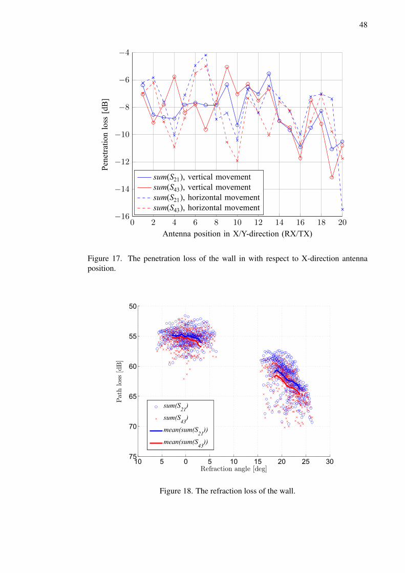
48

0 2 4 6 8 10 12 14 16 18 20−16

−14

−12

−10

−8

−6

−4

Antenna position in X/Y-direction (RX/TX)

Penetrationloss[dB]

sum(S21), vertical movementsum(S43), vertical movementsum(S21), horizontal movementsum(S43), horizontal movement

Figure 17. The penetration loss of the wall in with respect to X-direction antennaposition.

−10 −5 0 5 10 15 20 25 30−75

−70

−65

−60

−55

−50

Refraction angle [deg]

Path

loss

[dB]

sum(S21)

sum(S43)

mean(sum(S21))

mean(sum(S43))

Figure 18. The refraction loss of the wall.

49

4.5. Diffraction around a building corner

The measurement system can be used also for diffraction measurement. When movingvirtual antennas along the x-axis by distance of fractions of the wavelength, we can fastperform several measurement and see the effect of diffraction for the recorded impulseresponse. Also the changes in polarization due to the diffraction can be constructedfrom the measurement results. The results and further analysis of this measurement arepublished in [35] in the first international conference on 5G for ubiquitous connectivity(5GU) in November 26.− 28. 2014.

50

5. DISCUSSION

Accuracy and applicability for the different kind of measurements are just an examplesabout the characteristics describing how we have succeeded in building the system. Inthe final measurement system, there are many sources of inaccuracy. Hence, thereare many improvements that could be made for the system to increase the speed per-formance, dynamic range and applicability for different kind of measurements. Theverification measurements showed that we should always plan well the measurementsin order to be able to calculate specific measurement settings for each measurements.This was taken into account in the programming phase by parameterizing the inputparameters such that they could be chosen by the user. In this chapter we will evaluatethe measurement system and propose a number of improvements for the system whichof many will be implemented to the system in near future.

5.1. Evaluation of the system

When evaluating the measurement system, many sources of inaccuracy must be takeninto account. As discussed previously in the Section 3.1, the dynamic range availableand the total measurement time are inversely proportional to each other. The optimiza-tion of the parameters affecting to the measurement time and dynamic range shouldalways be done with respect to the current measurement scenario. This is why manyof the measurement settings such as IF-bandwidth of the VNA, source power of theVNA ports and the maximum speeds of the stepper motors are parameterized in themeasurement control software. By choosing the parameters correctly, the user can op-timize the measurement time with respect to the dynamic range requirements neededin each measurement scenario individually. Possibility to add the external amplifiersto the measurement chain were wanted to be made as an option. This is because theyare not necessarily needed in every case.

One drawback of the measurement setup is the antenna shaking, especially in hori-zontal movement. The shaking was estimated to be even several millimeters at worst,which could mean significant inaccuracy in location compared to the wavelength at10 GHz. The antenna shaking was compensated by making better acceleration anddeceleration ramps for the stepper motors. However, that slows down the measure-ment. Also, we added an optional offset delay for the both directions in the XY-gantryas an option in the measurement control software. The user can choose by himself ifhe uses the external delay or lower acceleration and deceleration ramps to prevent theantenna shaking. Best way to avoid the shaking would be to update the antenna mastto a stronger structure than it is now. For example, we could add additional structuresto support the mast and reduce shaking. One could also add acceleration sensors nearto the antenna to detect if the antenna is steady enough for the next measurement.

Another serious drawback in the system is the poor error and interrupt control. Theerror control in very long measurements where tens of thousands of VNA sweeps areperformed, is a very good way to prevent to corrupt the measurement data and causeproblems even during the measurements. The used limit switches ensures that thecarriage stays inside the allowed region of the XY-gantry. However, if the stepperis, for some reason, switched off during the measurement, the limit switch interrupt

51

routine may vanish from the stepper memory. The problem was overcame by definingthe limit switches in the measurement control software in the moving program.

The maximum moving range in the XY-gantry is 39 cm in horizontal direction and38 cm in vertical direction. In 10 GHz, this corresponds 26 antenna elements in hor-izontal, and 25 in vertical direction, if the antenna spacing of half of the wavelengthwas used. Thus, large antenna arrays up to 650 · 650 MIMO can be measured. In total,it could be said that there are several properties in the current system which we havesucceeded to implement. Many improvements that are proposed in the next Sectionare just proportions and there are not necessarily needed to be implemented.

5.2. Improvements proposed to the system

There are a number of ways to improve the measurement system by optimizing themeasurement time and adding new options to the system that can be chosen by theuser. To make the further analysis of the measurement results smoother in the future,an external analysis software could be made to analyze the wanted results right afterthe measurements. For the user, this would give an opportunity to change parameterswhile measuring and thus be able to improve the results.

From the user point of view, graphical user interface (GUI) would clarify better theoptions supported by the system. Also, it would give a better impression to the user thatwhat is going on in the system. MATLAB has a very good GUI tool, which could beused for building the user interface. Same subroutines which was made for the currentsystem could be applied. GUI would also give possibility to make for example pauseoption for the system such that user could pause the long measurements if needed.

In the channel measurements, the location of the antennas should always be able tobe measured with a good precision. When going higher in the frequency spectrum, theposition accuracy may became even more important. To make the location measure-ment automatic, programmable laser distance meters could be used by attaching themto the antenna mast structure. It could be possible to read the distance data automati-cally and store them within the measurement data. This would make further analysis ofthe results easier and data fitting could even be made during the measurements. Alsofor example global position system (GPS) -coordinate could be recorded if for exampleVNA has an internal GPS-receiver, which is the case for many devices. However, theprecision of the location measured by GPS is not very precise, but it could still be usedto rough estimation of the measurement location and thus help the future analysis. Onthe other hand, all external measurements, such as distance data read from the distancemeters increases the measurement time, especially if the data is read between each an-tenna positions. The usage of them should be able to be selected by user to be optional.Making improvements by adding the new options would also increase the prize of thesystem, which is not the aim if the system is wanted to pay itself back in the future bygiving good measurement results.

One problem in the current system is that it is only capable to measure planar antennaconfigurations. However, at the indoor-measurements, base station antennas are oftenplanar arrays which supports our implementation. Furthermore, the used antennas arenot able to receive signals from the backside beam. One proportion is that we coulduse a programmable rotary table or a herringbone gear to rotate the XY-gantry. This

52

would also give an opportunity to measure to different directions even with highlydirectional antennas, which was not possible with the current system. However, thisis not needed, if we would use omnidirectional dipole antenna in both ends. For someapplications, dipole antennas could be a good choice, but for example in diffraction orwall penetration loss measurements, it is better to use directional antennas. Off course,it is easy to replace the current antennas by different ones if needed.

One possibility is to insert a small rotary table or other rounding mechanics on topof the build XY-gantry and insert also a external linear stage on top of the rotary unitto move the antenna vertically. The rotator and the vertical linear stage would thenbe used to represent virtual cylindrical antenna array and the XY-gantry could be usedto move the whole antenna array. This would also make it possible to make virtual3-dimensional antenna arrays.

During the measurements, we also faced a problem in setting the origin of the an-tenna array. It would be useful, if the origin could be freely chosen into the XY-gantryfor both end separately. This option could be quite easily implemented and will beavailable to the next version of the measurement system.

One way to cancel the effect of antennas out from the measurement results could beto use fixed reference antenna in RX end. The measured reference path loss could befor example used as a reference value for the data measured in different antenna loca-tions. However, the usage of reference antenna can be replaced by external referencemeasurements. This, however can only be done, if the channel is assumed to be timeinvariant and thus the same in real measurement and reference measurement.

5.3. About the measurements

The verification measurements were done mostly to verify the system operation andgive an reference and test data for the DoA and DoD algorithms which will be part ofthe measurement system in the final product. In these measurements, it was clearlyseen that the reflection rotates the polarization vector and thus some of the powerof the reflected component is leaked to the other polarization domain. This may besignificant for example, when considering separating users in the polarization domain.It is clear that the reflection is one of the most dominating propagation phenomena atthe indoor environment. The anechoic chamber scenario gave a very good reference forthe further measurements. The results implied that the system does not cause internalspurious response for the results.

The test measurements performed in the class room was in reality the first measure-ment scenario performed with this system. Thus, there were many unsure things inthe measurement control software and the system itself which had never been testedbefore. The bug in the code discussed in the Section 4.3 did cause corrupted data be-cause of wrong calibration pool in the VNA channel 1. The calibration problem waslater on corrected. Anyway, the measurements gave an valuable information aboutthe wave behavior in the class room environment. Also the recorded data has beenused to test the angle algorithms for a multipath environment. Yet, the results couldbe analyzed further to calculate channel parameters such as delay spreads and angularspreads. However, several RX positions should be considered in order to calculate forexample path loss exponent for the environment.

53

The wall penetration loss in 10 GHz is important especially for calibrating RT toolsto produce a 3D channel model about the room. As it was seen in the measurements,the penetration loss of the wall may vary even 8 dB depending on the part of the wallunder test. To be able to calculate trustable mean penetration loss of such wall, weshould perform several measurements for similar walls and compare them. Indoorwalls might have many different kind of structures which causes huge variations forthe penetration loss. If the wall is made of concrete, the way how the wall was masoned(e.g. water concentration used for concrete) affects directly to its electromagnetic prop-erties. For the nonorthogonal wave incidence with respect to the surface of the wall,the penetration loss was also observed to vary a lot. For making a theoretical modelfor the wall, we should study better the real structure of the wall.

54

6. SUMMARY

The goal of this thesis was to build a MIMO channel measurement system by using fourport vector network analyzer and virtual antenna arrays in both TX and RX ends. Thebuilt system measures each single antenna channel separately. The radio propagationenvironment was assumed to be static during the recordings. A dual polarized patchantenna with two feeding ports was used as an antenna element. The linear stages andprogrammable stepper motors were utilized to build an XY-gantry to move the antennaelement in one plane. All of the measurement equipment were controlled by the samecentralized measurement control software.

The system was able to measure antenna configurations up to 26 antenna elementsin the horizontal and 25 elements in the vertical direction, respectively, assuming afrequency of 10 GHz and antenna spacing of half of a wavelength. The measurementtime for one single antenna channel was 1.9 s in the horizontal direction and 0.9 s inthe vertical direction, respectively. The longer measurement time for the horizontalmovement was caused by the external waiting to prevent the vibrations of the antennaduring the measurement.

Three channel measurement scenarios and their initial results were presented to ver-ify the system operation and to demonstrate the system applicability for the differentcases. A verification measurement was performed in the anechoic chamber to verifythat the system did cause any internal spurious responses to the results. The next mea-surement was performed in a classroom to demonstrate the multipath propagation envi-ronment. The reflection, diffraction and LOS propagation phenomena were concludedto be the most dominating propagation phenomena in the classroom. Furthermore, anindoor wall penetration loss measurement from the classroom to another was made toshow that the measurement system could also be applied for the measurements requir-ing an accurate antenna shifting between the measurement points. The result of thismeasurement was that the wall penetration loss may vary drastically depending on partof the wall under test. The penetration loss of the measured wall was varied between5 and 13 dB. The results measured with this setup could be used for angular domainalgorithms to estimate the direction of arrival and departure, respectively. The mea-surement system was concluded to be able to make successful measurements in thetested propagation environments. The measurement system will be applied for variousMIMO radio channel measurement scenarios at 10 GHz and beyond.

55

7. REFERENCES

[1] Massive MIMO Info Point (accessed 25.8.2014). URL: www.massivemimo.eu.

[2] International Telecommunication Union official website (accessed 25.8.2014).URL: http://www.itu.int/en.

[3] Goldsmith A. (2005) Wireless Communications. Cambridge University Press,first ed., 46 - 48 p.

[4] Hoydis J., Hoek C., Wild T. & ten Brink S. (2012) Channel Measurements forLarge Antenna Arrays. In: International Symposium on Wireless CommunicationSystems (ISWCS), 2012, pp. 811–815.

[5] The Essentials of Vector Network Analysis; From α to Z0. Anritsu Company,2007.

[6] Payami S. & Tufvesson F. (2012) Channel Measurements and Analysis for VeryLarge Array Systems at 2.6 GHz. In: Sixth European Conference on Antennasand Propagation (EUCAP), 2012, pp. 433–437.

[7] Ranvier S., Kivinen J. & Vainikainen P. (2007) Millimeter-Wave MIMO RadioChannel Sounder. IEEE Transactions on Instrumentation and Measurement 56,pp. 1018–1024.

[8] Abouraddy A. & Elnoubi S. (2000) Statistical modeling of the indoor radio chan-nel at 10 GHz through propagation measurements. I. Narrow-band measurementsand modeling. IEEE Transactions on Vehicular Technology 49, pp. 1491–1507.

[9] Kim M., Konishi Y., Chang Y. & Takada J.I. (2014) Large Scale Parametersand Double-Directional Characterization of Indoor Wideband Radio MultipathChannels at 11 GHz. IEEE Transactions on Antennas and Propagation 62, pp.430–441.

[10] Fleisch D. (2008) A Student’s Guide to Maxwell’s Equations. Cambridge Uni-versity Press.

[11] Pozar D.M. (2005) Microwave Engineering. John Wiley & Sons, third ed.

[12] Bertoni H.L. (2000) Radio Propagation for Modern Wireless Systems. PrenticeHall PTR.

[13] Balanis C.A. (2005) Antenna Theory - Analysis and Design. John Wiley & Sons,third ed.

[14] Räisänen A. & Lehto A. (2003) Radio Engineering for Wireless Communicationand Sensor Applications. Artech House.

[15] Miquel A.C. (2009) UWB antenna design for underwater communications. Mas-ter’s thesis, Delft University of Technology.

56

[16] Lindell I. (1996) Radioaaltojen Eteneminen. Otatieto, fourth ed.

[17] Saunders S. & Aragón-Zavala A. (2007) Antennas and Propagation for WirelessCommunication Systems. John Wiley & Sons, second ed.

[18] ITU-R Recommendation P.526-7: Propagation by diffraction (accessed13.10.2014). URL: \urlhttps://www.itu.int/dms_pubrec/itu-r/rec/p/R-REC-P.526-7-200102-S!!PDF-E.pdf.

[19] Parsons J. (2000) The Mobile Radio Propagation Channel. John Wiley & Sons.

[20] Phillips C., Parr J. & Riskin E. (2013) Signals, Systems, & Transforms. PearsonEducation.

[21] Rohde & Schwarz ZNB/ZNBT Vector Network Analyzer; User manual (accessed25.8.2014). URL: http://www.rohde-schwarz.com/en/manual/r-s-znb-znbt-user-manual-manuals-gb1_78701-29151.html.

[22] Sundararajan D. (2001) The Discrete Fourier Transform: Theory, Algorithms andApplications. World Scientific Publishing Company, Incorporated.

[23] Chu E. (2012) Discrete and Continuous Fourier Transforms: Analysis, Applica-tions and Fast Algorithms. Taylor & Francis.

[24] Miteq LCN-0812 amplifier datasheet (accessed 13.10.2014). URL:\urlhttps://www.miteq.com/viewmodel.php?model=LCN-0812.

[25] Hittite HMC-C026 amplifier datasheet (accessed 13.10.2014). URL:\urlhttp://www.hittite.com/content/documents/data_sheet/hmc-c026.pdf.

[26] R&S ZV-Z5x electonic calibration kit datasheet (accessed 13.10.2014).URL: \urlhttp://rosenkranz-elektronik.de/shop/datenblaetter/R+SZV-Z5x_datasheet.pdf,.

[27] Understanding the VNA calibration, Anritsu (accessed13.10.2014). URL: \urlhttp://anlage.umd.edu/Anritsu_understanding-vna-calibration.pdf.

[28] Lexium MDrive Ethernet TCP/IP products LMDxE/N57 and LMDxE/N85;Product hardware manual (accessed 25.8.2014). URL: http://motion.schneider-electric.com/lmd/downloads/literature/LMDE.pdf.

[29] Programming and Software Reference for Lexium MCode and Lex-ium Mcode/TCP (accessed 25.8.2014). URL: http://motion.schneider-electric.com/lmd/downloads/literature/MCode_LMD.pdf.

57

[30] Hiwin KK-linear stage dataheet (accessed 25.8.2014). URL: http://hiwin.com/pdf/ls/Single%20Axis%20Robot_K02TE02-0701_311.pdf.

[31] Panasonic GX-F12A-P inductive sensor datasheet (accessed 25.8.2014). URL:http://www.farnell.com/datasheets/1809919.pdf, publisher=Panasonic EW.

[32] MATLAB Instument Control Toolbox; Users Quide (accessed 25.8.2014). URL:http://www.mathworks.se/help/instrument/index.html.

[33] Lexium MCode Programming and Software Reference, Schneiderelectric (accessed 13.10.2014). URL: \urlhttp://motion.schneider-electric.com/lmd/downloads/literature/MCode_LMD.pdf.

[34] Chen Z., Gokeda G. & Yu Y. (2010) Introduction to Direction-of-arrival Estima-tion. Artech House.

[35] Tervo N., Dias C., Hovinen V., Sonkki M., Roivainen A., Meinilä J. & Latva-ahoM. (2014) Diffraction Measurements around a Building Corner at 10 GHz. In:First International Conference on 5G for Ubiquitous Connectivity (5GU), IEEE2014.

58

8. APPENDICES

Appendix 1 The wiring of the VNA-based measurement setup

Appendix 2 Flow chart of the subroutine for finding the limit switches

Appendix 3 Flow chart of the moving program for steppers

Appendix 4 The flow chart of the VNA initialization

Appendix 5 Selectable input parameters for the measurement control software

Appendix 6 The flow chart of the main program controlling the measurements

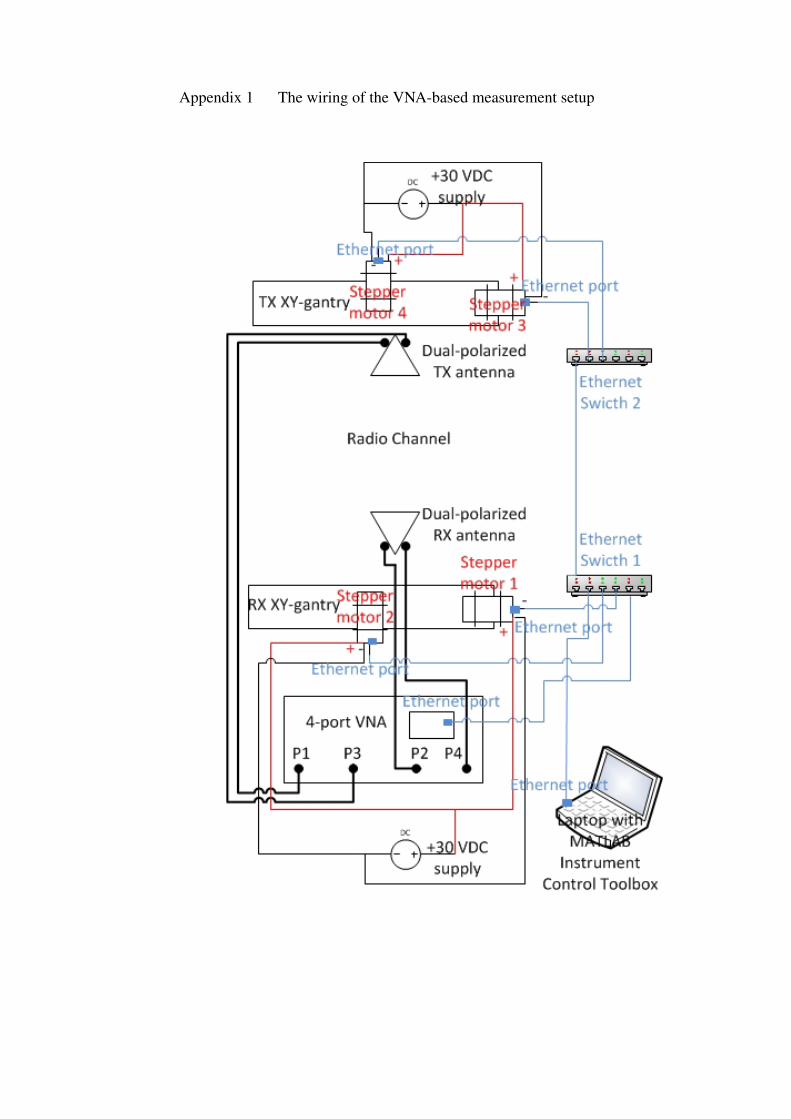
Appendix 1 The wiring of the VNA-based measurement setup

Appendix 2 Flow chart of the subroutine for finding the limit switches

Start Program

Define input 1 as positive limit

Flush the object input

Define limit stop mode to be ”LM =

4"

Define input 2 as negative limit

Move stepper 20000 microsteps to

positive diretion

Move to negative direction

Move the amount of offset to positive

direction

Stop movement

Clear error register

Set P = 0

I2 active?

End program

Yes

No

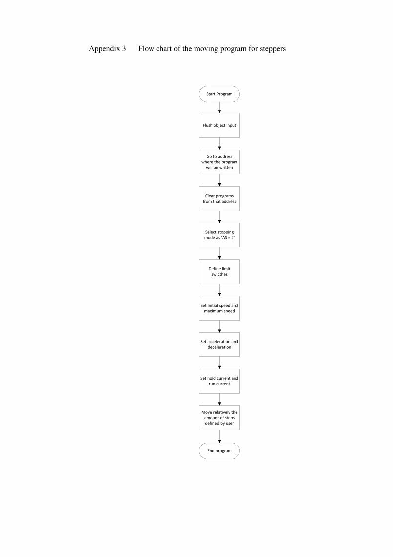
Appendix 3 Flow chart of the moving program for steppers

Start Program

Flush object input

Go to address where the program

will be written

Clear programs from that address

Select stopping mode as ’AS = 2'

Define limit swicthes

Set Initial speed and maximum speed

Set acceleration and deceleration

Set hold current and run current

Move relatively the amount of steps defined by user

End program

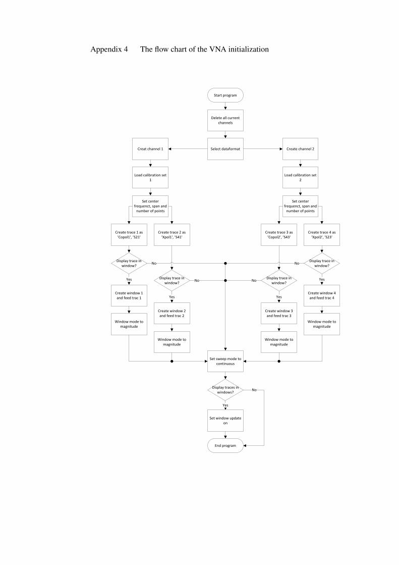
Appendix 4 The flow chart of the VNA initialization

Start program

Delete all current channels

Select dataformatCreat channel 1 Create channel 2

Create trace 1 as ’Copol1', ’S21'

Create trace 2 as ’Xpol1', ’S41'

Create trace 4 as ’Xpol2', ’S23'

Create trace 3 as ’Copol2', ’S43'

Set center frequenct, span and

number of points

Load calibration set 2

Load calibration set 1

Set center frequenct, span and

number of points

Display trace in window?

Display trace in window?

Display trace in window?

Create window 3 and feed trac 3

Create window 4 and feed trac 4

Create window 2 and feed trac 2

Create window 1 and feed trac 1

Display trace in window?

Display traces in windows?

Set window update on

Set sweep mode to continuous

End program

Window mode to magnitude

Window mode to magnitude

Window mode to magnitude

Window mode to magnitude

Yes

Yes

Yes

No

Yes

Yes

No No

No No

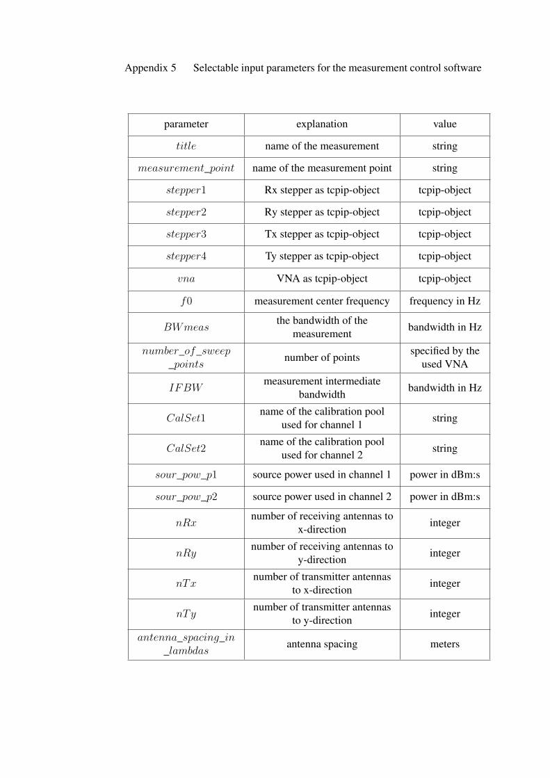
Appendix 5 Selectable input parameters for the measurement control software

parameter explanation value

title name of the measurement string

measurement_point name of the measurement point string

stepper1 Rx stepper as tcpip-object tcpip-object

stepper2 Ry stepper as tcpip-object tcpip-object

stepper3 Tx stepper as tcpip-object tcpip-object

stepper4 Ty stepper as tcpip-object tcpip-object

vna VNA as tcpip-object tcpip-object

f0 measurement center frequency frequency in Hz

BWmeasthe bandwidth of the

measurementbandwidth in Hz

number_of_sweep_points

number of pointsspecified by the

used VNA

IFBWmeasurement intermediate

bandwidthbandwidth in Hz

CalSet1name of the calibration pool

used for channel 1string

CalSet2name of the calibration pool

used for channel 2string

sour_pow_p1 source power used in channel 1 power in dBm:s

sour_pow_p2 source power used in channel 2 power in dBm:s

nRxnumber of receiving antennas to

x-directioninteger

nRynumber of receiving antennas to

y-directioninteger

nTxnumber of transmitter antennas

to x-directioninteger

nTynumber of transmitter antennas

to y-directioninteger

antenna_spacing_in_lambdas

antenna spacing meters

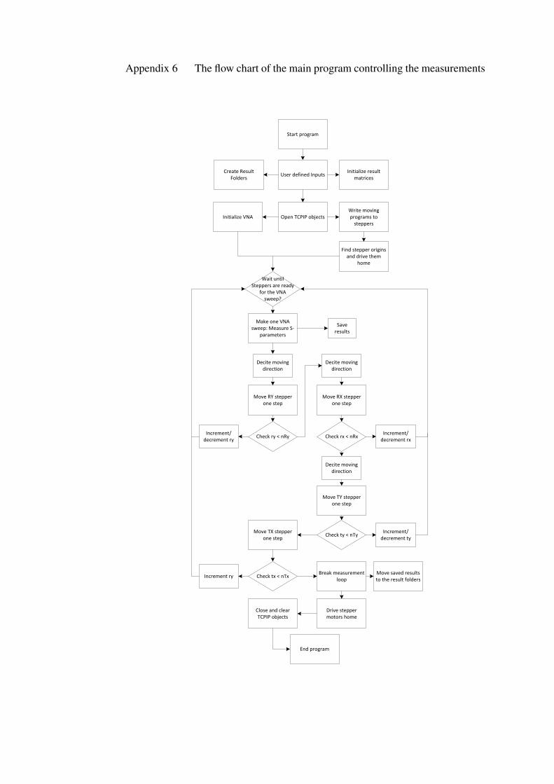
Appendix 6 The flow chart of the main program controlling the measurements

User defined InputsCreate Result

Folders

Open TCPIP objectsInitialize VNA

Initialize result matrices

Find stepper origins and drive them

home

Write moving programs to

steppers

Wait until Steppers are ready

for the VNA sweep?

Make one VNA sweep: Measure S-

parameters

Save results

Move RX stepper one step

Move RY stepper one step

Move TX stepper one step

Check ry < nRyIncrement/

decrement ry

Decite moving direction

Decite moving direction

Check rx < nRx

Decite moving direction

Move TY stepper one step

Check ty < nTy

Increment/decrement rx

Increment/decrement ty

Check tx < nTxIncrement ryBreak measurement

loop

Drive stepper motors home

Close and clear TCPIP objects

End program

Start program

Move saved results to the result folders