Embed Size (px)
Citation preview

Institut für Feuerungs- und Kraftwerkstechnik Direktor: Prof. Dr. techn. G. Scheffknecht
Pfaffenwaldring 23 • 70569 Stuttgart
Tel. +49 (0) 711-685 63487 • Fax +49 (0) 711-685 63491
Master Thesis Nr. 3350
cand. M.Sc Mario Ruiz
Assessment of Calcium Looping as a solution for CO2 capture in
the steel production process
-
Machbarkeitsuntersuchung für das Calcium Looping Verfahren zur
CO2 Abscheidung in der Stahlerzeugung
Anschrift: Hostafrancs de Sio 4 08014, Barcelona, Spain Ausgabe: 1.12.2014 Abgabe: 31.05.2015 Betreuer: Dipl.-Ing. Heiko Dieter

II
I would like to express my gratitude to my supervisor Heiko Dieter for the opportunity to work in this topic and for all the help and advice supported during these months. I would like also to thank Christopher Pust and the company Rheinkalk. Furthermore I would like to thank Marcel Beirow and the DEU department for the help given.

List of contents IV
Abstract V
Abstract
In this study a first assessment of the utilization of the Calcium Looping (CaL) as a CO2
capture method in the steel production process has been done. The applicability of CaL for
CO2 capture from the blast furnace gas of the Top Gas Recycling Blast Furnace (TGR-BF)
proposed by ULCOS has been studied.
Data of previous experimental campaigns where CaL was tested for post-combustion
capture in a 200 kWth pilot plant has been used to simulate in Aspen PlusTM the CaL working
under the TGR-BF conditions. The results of the CaL simulation have been used to compare
CaL with VPSA, proposed by ULCOS as CO2 capture method, and amines adsorption
(MDEA), presented by the IEAGHG. The three technologies have been energetically
compared and its integration in a reference steel mill has been studied, offering CaL the
advantage that is able to meet the electricity demand of the steel mill, avoiding the
requirement of an additional power plant. As a direct consequence, the CO2 emissions in the
CaL steel mill can be strongly reduced in comparison with the other capture technologies.
A determination of the costs of the CaL plant has been carried out and an economic
comparison of the cost of steel production and the cost of CO2 avoidance for the different
capture technologies has been done. The results showed that for the proposed steel mill and
under the assumptions done, CaL offers the lowest CO2 avoidance cost.
Kurzfassung
In diesem Projekt wird die Benutzung des Calcium Looping Verfahrens zur CO2-Abscheidung
in der Stahlindustrie untersucht. Eine Machtbarkeitsuntersuchung zur CO2-Abscheidung aus
dem Gichtgas des Top Gas Recycling Hochofens mit CaL wurde durchgeführt. Diese TGR-
BF Technik mit VPSA für CO2-Abscheidung ist im ULCOS Programm entstanden. In dieser
Arbeit werden experimentelle Ergebnisse aus 200 kWth Pilotversuchen benutzt um CaL in
Aspen PlusTM zu simulieren. Anhand der Simulationsergebnisse wurde CaL mit VPSA und
MDEA verglichen. Die drei Techniken wurden energetisch bewertet und die Integration in ein
Stahlwerk wurde untersucht. Das CaL hat den Vorteil, dass es genug Strom für das ganze
Stahlwerk erzeugen kann. Deshalb wird kein zusätzliches Kraftwerk benötigt. Aus diesem
Grund, können die CO2-Emissionen stark reduziert und niedriger werden als mit den anderen
Techniken zur CO2-Abscheidung.
Die Kosten des CaL wurden geschätzt und die Wirtschaftlichkeit der drei Stahlwerke wurde
ermittelt. Die gesamten Stahlgestehungskosten und die CO2-Vermeidungskosten wurden für
die drei Stahlwerke kalkuliert.

List of contents VI
List of contents
Abstract ................................................................................................................................. V
Kurzfassung .......................................................................................................................... V
List of Figures ...................................................................................................................... XII
List of Tables ....................................................................................................................... XII
1 Introduction .................................................................................................................... 1
1.1 Steel industry emissions .......................................................................................... 1
1.2 Short term CO2 emission reduction technologies in the blast furnace ...................... 2
1.2.1 Usage of biomass ............................................................................................ 3
1.2.2 Substitution of CO by H2 as a reducing agent ................................................... 3
1.2.3 Electrolysis ....................................................................................................... 3
1.2.4 Top gas recycling ............................................................................................. 3
1.3 ULCOS project ........................................................................................................ 4
1.4 Assignment and goal setting ................................................................................... 4
2 Theoretical fundamentals ............................................................................................... 6
2.1 Fundamentals of the steel production ...................................................................... 6
2.1.1 Basic principles of a steel mill ........................................................................... 6
2.1.2 Blast furnace process ....................................................................................... 8
2.1.3 Main reactions and components of the BF ....................................................... 9
2.1.4 Products ..........................................................................................................10
2.1.5 Integration of the Blast furnace with steam cycle .............................................11
2.2 ULCOS Top Gas Recycling Blast Furnace .............................................................11
2.3 Alternative post-combustion CO2 capture technologies...........................................13
2.3.1 VPSA technology ............................................................................................13
2.3.2 MDEA/Piperazine ............................................................................................13
2.4 Calcium Looping Process .......................................................................................14
2.4.1 Description of the process ...............................................................................14
2.4.2 The calcium oxide-carbon dioxide equilibrium .................................................15
2.4.3 Energy recovery ..............................................................................................16
2.4.4 Characteristics of the CaL process ..................................................................16
2.4.5 Adsorption-Enhanced Reforming.....................................................................18
List of contents VII
2.4.6 Reactivity of the CaO particles ........................................................................18
2.5 Other processes .....................................................................................................20
2.5.1 Air Separation Unit ..........................................................................................20
2.5.2 CO2 conditioning and storage ..........................................................................21
2.6 Fundamentals of the economic analysis .................................................................22
2.6.1 Price basis ......................................................................................................22
2.6.2 Interest rate .....................................................................................................22
2.6.3 Plant life and construction period.....................................................................22
2.6.4 Capital costs ...................................................................................................23
2.6.5 Operating costs ...............................................................................................24
2.6.6 Cost of steel production ...................................................................................25
3 Simulation of the CaL process .......................................................................................27
3.1 Aspen PlusTM Simulator ..........................................................................................27
3.1.1 Reactor models in Aspen PlusTM .....................................................................27
3.1.2 Coal definition .................................................................................................27
3.2 Basic simulation without heat integration ................................................................28
3.2.1 General assumptions ......................................................................................29
3.2.2 Description of the basic CaL model .................................................................30
3.2.3 RStoic carbonator ...........................................................................................32
3.2.4 Results of the basic model ..............................................................................34
3.3 Energy integration ..................................................................................................36
3.3.1 Simulation in Aspen PlusTM .............................................................................39
3.3.2 Results of the simulation with heat integration .................................................39
3.4 CO2-lean treatment and injection ............................................................................40
3.5 CO2 recirculation in the combustor .........................................................................42
3.6 Calculation of the electricity generated in the CaL Process ....................................43
4 Energetic comparison of CO2 capture technologies .......................................................46
4.1 General statements ................................................................................................46
4.1.1 Energetic cost of CaL CO2 capture ..................................................................47
4.2 Energetic cost of capture of the different CCS technologies ...................................49
5 Implementation of the CaL in the steel mill ....................................................................51
5.1 Scaling of the plant .................................................................................................51
5.2 Reference steel mill ................................................................................................52

List of contents VIII
5.2.1 Electricity consumptions and producers in the steel mill ..................................52
5.2.2 Steam Generation Plant ..................................................................................54
5.3 Steel mill with Top Gas Recycling Blast Furnace (TGR-BF) and CaL CO2 capture .55
5.4 Steel mill with TGR-BF and VPSA CO2 capture ......................................................57
5.5 CO2 emissions in the Steel mill ...............................................................................57
6 Cost of the Calcium Looping plant .................................................................................62
6.1 Capital costs of the CaL facility ..............................................................................62
6.1.1 Operating costs ...............................................................................................67
6.2 Fuel costs ...............................................................................................................68
6.3 Limestone costs .....................................................................................................68
7 Economic comparison with other CO2 capture technologies ..........................................69
7.1 Investment costs comparison .................................................................................69
7.2 Operating costs ......................................................................................................72
7.2.1 Fixed cost ........................................................................................................72
7.2.2 Variable cost ...................................................................................................73
7.3 Cost of steel production ..........................................................................................76
8 Conclusions ...................................................................................................................79
9 Appendix .......................................................................................................................81
9.1 Hydrogen production through AER .........................................................................81
9.1.1 Simulation in Aspen PlusTM .............................................................................81
9.2 Flow sheets of Aspen PlusTM simulation .................................................................84
9.3 Operating costs of the reference steel mill ..............................................................87
9.3.1 Maintenance costs ..........................................................................................87
9.3.2 Labour costs ...................................................................................................87
9.3.3 Energy and reductant ......................................................................................88
9.4 Chemical Engineering Plant Cost Index (CEPCI) ...................................................89
10 References ................................................................................................................90
Nomenclature IX
Nomenclature
Symbol Explanation Unit
𝐴𝑀 Annual amortization €
𝐶 Investment cost of the unit €
𝐶0 Investment cost of the reference unit €
𝐶𝑅𝐹 Capital Recovery Factor -
��𝑂2 Oxygen mass flow consumption in regenerator kgO2/s
��𝐶𝑂2 CO2-rich mass flow for compression kg/s
Pel,gross Electrical power gross produced in CaL kW
ηel,gross Electric conversion efficiency %
𝐶𝐶𝑛 Capital costs for n-year €
𝐶𝑂2 𝐸𝑚𝐶𝑎𝑝𝑡𝑢𝑟𝑒 𝑆𝑀 Total CO2 emission steel mill with CO2 capture kg CO2/t HRC
𝐶𝑂2 𝐸𝑚𝑅𝑒𝑓𝑆𝑀 Total CO2 emission reference steel mill kg CO2/t HRC
𝐶𝑆𝑡𝑒𝑒𝑙 𝑃𝑟𝑜𝑑𝑢𝑐𝑡𝑖𝑜𝑛 Cost of steel production €/ton steel
𝐶𝑐𝑜𝑛𝑠 Personal contribution by the building owners €
𝐶𝑖𝑛𝑠 Total cost of the installation €
𝐸𝐴𝑆𝑈 Energy consumed by the air separation unit kWh/kgO2
𝐸𝐶 Fraction of external capital -
𝐸𝐶𝑂2 CO2 capture efficiency -
fa Fraction of active CaO -
𝐹𝐶𝑂2 Inlet molar flow of CO2 in the carbonator mol/s
𝐹𝐶𝑂2𝑖𝑛 Inlet molar flow of CO2 in the carbonator mol/s
𝐹𝐶𝑂2𝑜𝑢𝑡 Outlet molar flow of CO2 in the carbonator mol/s
𝐹𝐶𝑎𝐶𝑂3 Molar flow of fresh limestone mol/s
𝐹𝐶𝑎𝑂 Molar flow entering the carbonator mol/s
𝑘 Construction time years
𝑖𝑐 Interest during construction time %
𝐼𝐶 Fraction of internal capital -
𝐼𝐷𝐶 Interest generated during planning and
construction of the installation
€
𝑖𝐸𝐶 Interest of the external capital %
𝑖𝐼𝐶 Interest of the internal capital %
𝐼𝑃𝑛 Interest payment for n-year €
𝑖𝑟 Real interest %
𝐼𝑡𝑜𝑡 Total investment costs €
Nomenclature X
𝐼𝑋 Investment cost of unit x €
𝐿𝐴𝑁 Levelized annual costs €
𝐿𝑅 Looping ratio molCaO/molCO2
𝑚 Decreasing cost factor -
𝑛 Life of the project years
𝑛. 𝑎𝑙𝑙𝑜𝑐𝑎𝑡𝑖𝑜𝑛 Fraction of the construction costs in year n %
OCfix Fixed operating costs €
OCsp, fixed Specific operating costs €/kW
OCvar Variable operating costs €/MWhel
𝑃 Size of the unit -
𝑃𝐶𝑂2 𝑐𝑜𝑚𝑝𝑟𝑒𝑠𝑠𝑖𝑜𝑛 Power required for CO2 compression kW
𝑃𝐶𝑎𝐿,𝑜𝑤𝑛 Own electrical consumption in CaL kW
𝑃0 Size of the referent unit -
𝑃𝑉𝑇𝐶 Present value of the total costs €
𝑃𝑒𝑙,𝑛𝑒𝑡 Electrical power net produced in CaL kW
𝑄th Total energy extracted for steam production MW
𝑡 𝐻𝑅𝐶 Tons of Hot Rolled Coil tons
𝑡ℎ𝑚 Tons of Hot Metal tons
𝜏 Cabonator space time s
𝑋𝑐𝑎𝑙𝑐 Carbonate content in/after the regenerator molCaCO3/molCa
𝑋𝑐𝑎𝑟𝑏 Carbonate content in/after the carbonator molCaCO3/molCa
𝑋𝑚𝑎𝑥 Maximum carbonation conversion -
𝑋𝑠𝑢𝑙𝑓 Fraction of active CaO reacting with sulfur -
𝑍𝑛 Interest generated for n-year of the construction
period
€
Acronyms Explanation
AER Adsorption-Enhanced Reforming
BF Blast Furnace
BFG Blast Furnace Gas
BOF Basic Oxygen Furnace
BOFG Basic Oxygen Furnace Gas
CCS Carbon Capture and Storage
DFB Dual Fluidized Bed
DRI Direct Reduced Iron
EAF Electric Arc Furnace route
EBF Experimental Blast Furnace

Nomenclature XI
ECSC European coal and Steel Community
HBI Hot Briquetted Iron
HRC Hot Rolled Coil
IEA International Energy Agency
IEAGHG International Energy Agency Greenhouse Gas R&D Programme
ISM Integrated Steel Mill
LRI Low Reduced Iron
MDEA/Pz Methyl-Di-Ethanol Amine activated with Piperazine
MDEA Methyl-Di-Ethanol Amine
MEA Monoethanolamine
OBF Oxy-Blast Furnace
Pz Piperazine
RFCS Research Fund for Coal and Steel
SM Steel Mill
TGR-BF Top Gas Recycling Blast Furnace
TRG Top Gas Recycling
ULCOS Ultra Low CO2 Steelmaking
VPSA Vacuum Pressurized Swing Adsorption

List of Figures and Tables XII
List of Figures
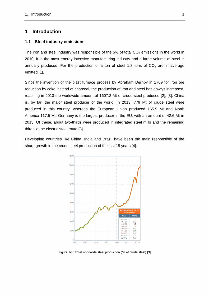
Figure 1-1: Total worldwide steel production (Mt of crude steel) [3] ....................................... 1
Figure 1-2: Evolution of the consumption of reducing agent in the Blast Furnace .................. 2
Figure 2-1: Flow diagram of the main processes in an ISM ................................................... 7
Figure 2-2: Breakdown of the CO2 production at a conventional integrated steel mill [6] ....... 8
Figure 2-3: Scheme of the inputs and outputs of a blast furnace[15] ..................................... 8
Figure 2-4: Flow sheet in Version 4 [18] ...............................................................................12
Figure 2-5: Principle of the Calcium Looping Process ...........................................................14
Figure 2-6: Equilibrium equations of the decomposition of CO2 [30] .....................................15
Figure 3-1: Flow diagram of the basic CaL process ..............................................................30
Figure 3-2: Carbonator represented with RStoic block ..........................................................32
Figure 3-3: Flowsheet of the basic simulation with RGibbs carbonator .................................33
Figure 3-4: Energy integration of the CaL treating BFG ........................................................38
Figure 3-5: Simulation of the pre-treatment of the process gas .............................................41
Figure 7-1: Cost of steel production for the different steel mills .............................................78
Figure 9-1: Sensitivity analysis of the composition of the CO2-lean gas against the S/C ratio
.............................................................................................................................................82
Figure 9-2: Aspen Plus sensitivity analysis. Molar flow of CO at the exit of the gasifier against
S/C ratio ...............................................................................................................................83
Figure 9-3: Aspen Plus sensitivity analysis. Molar flow of hydrogen at the exit of the gasifier
against S/C ratio ...................................................................................................................83
Figure 9-4: Aspen PlusTM flow sheet of the basic simulation using RStoic carbonator reactor
.............................................................................................................................................84
Figure 9-5: Aspen PlusTM flow sheet of the simulation with heat integration. Scenario with
CO2 recirculation into the regenerator ..................................................................................85
Figure 9-6: Aspen PlusTM flow sheet of the simulation introducing steam into the gasifier ....86
List of Tables
Table 2-1: Composition of the Coke Oven Gas [12] ............................................................... 7
Table 2-2: Oxygen requirements in the steel mill [IEA] .........................................................21
Table 3-1: Proximate analysis ..............................................................................................28
Table 3-2: Ultimate analysis .................................................................................................28
Table 3-3: Composition of the inlet Blast Furnace Gas [17] ..................................................29
Table 3-4: General assumptions of the simulation ................................................................30
Table 3-5: Flue gases compositions of the basic simulation with RGibbs carbonator ...........34

List of Figures and Tables XIII
Table 3-6: Consumptions in the regenerator using RGibbs carbonator .................................34
Table 3-7: Inlet and outlet flows of the carbonator ................................................................35
Table 3-8: Flue gases compositions of the basic simulation with RStoic carbonator .............36
Table 3-9: Consumptions in the regenerator using RStoic carbonator ..................................36
Table 3-10: Heat integration without CO2 recirculation .........................................................39
Table 3-11: Flue gas compositions with heat integration ......................................................40
Table 3-12: Outputs of the simulation with energy integration ...............................................40
Table 3-13: Process gas combusted for pre-heating ............................................................41
Table 3-14: Process gas reinjected into the blast furnace .....................................................41
Table 3-15: Heat integration with CO2 recirculation in the calciner ........................................42
Table 3-16: Main results of the simulation with CO2 recirculation in the regenerator .............43
Table 3-17: Electricity production in the two different scenarios ............................................45
Table 4-1: Comparison of CO2 capture technologies for an Integrated Steel Mill [11],
[12][12][12] ...........................................................................................................................46
Table 4-2: Energetic cost of CaL CO2 capture ......................................................................48
Table 4-3: Comparison of the energetic cost of capture for different CCS technologies ........49
Table 5-1: Characteristics of the reference steel mill ............................................................51
Table 5-2: Main flows of the CaL applied to the steel mill .....................................................52
Table 5-3: Summary of the energy produced in the CaL for the reference steel mill .............52
Table 5-4: Electricity demand and supply of the steel mill without and with CO2 capture[12]
[Table C-8] ...........................................................................................................................53
Table 5-5: Steam demand and supply of the steel mill without and with CO2 capture [12]
[Table C-9] ...........................................................................................................................54
Table 5-6: Electricity demand and supply of the steel mill with CaL CO2 capture ..................56
Table 5-7: Steam demand and supply of the steel mill with CaL CO2 capture .......................57
Table 5-8: Breakdown of CO2 emissions- Reference steel mill [12] ......................................59
Table 5-9: Breakdown of CO2 emissions- Steel mill using MDEA CO2 capture [12] ..............59
Table 5-10: CO2 emissions- Steel mill using VPSA CO2 capture ..........................................60
Table 5-11: Breakdown of CO2 emissions- Steel mill using CaL CO2 capture .......................61
Table 5-12: Summary of the total emissions of the steel mill using different CO2 capture
technologies .........................................................................................................................61
Table 6-1: Calculation of the carbonator reactor by [48] .......................................................62
Table 6-2: Investment cost of the carbonator for the case study ...........................................63
Table 6-3: Cost of the regenerator reactor ............................................................................64
Table 6-4: Cost of the ASU ...................................................................................................65
Table 6-5: Cost of the CO2 compression plant ......................................................................65
Table 6-6: Remaining investment costs ................................................................................66
List of Figures and Tables XIV
Table 6-7: Overview of the investment costs ........................................................................67
Table 6-8: Total investment costs of the CaL process ..........................................................67
Table 6-9: Operating costs of the CaL process .....................................................................68
Table 6-10: Fuel cost of the CaL process .............................................................................68
Table 6-11: Limestone costs of the CaL process ..................................................................68
Table 7-1: Investment costs of the steel mill without and with MDEA CO2 capture ...............69
Table 7-2: Investment costs of the steel mill with TGR-BF and VPSA CO2 capture ..............70
Table 7-3: Investment costs of the steel mill with TGR-BF and CaL CO2 capture .................71
Table 7-4: Fixed O&M costs of a steel mill with CaL and VPSA CO2 capture .......................72
Table 7-5: Fuel balance in the VPSA steel mill .....................................................................74
Table 7-6: Variable O&M costs of steel mill with CaL and VPSA CO2 capture ......................74
Table 7-7: Operating Costs of CaL and VPSA CO2 capture plant .........................................75
Table 7-8: Total annual O&M cost of the steel mill with CaL and VPSA CO2 capture plant ...75
Table 7-9: Comparison of the investment and operating costs of the different steel mills .....76
Table 7-10: Cost of steel production for the different steel mills ............................................76
Table 7-11: Breakdown of the total cost of steel production ..................................................77
Table 7-12: Cost of CO2 avoidance for the steel mills with CaL, VPSA and MDEA CO2
capture .................................................................................................................................78
Table 9-1: Composition of the CO2-lean gas (dry) leaving the gasifier ..................................82
Table 9-2: Maintenance costs of the reference steel mill without capture and with MDEA
capture. Table D-5 [12] .........................................................................................................87
Table 9-3: Labour costs of the reference steel mill without capture and with MDEA capture.
Table D-6 [12] ......................................................................................................................87
Table 9-4: Cost and consumption of coking and PCI coal of the reference steel mill without
capture and with MDEA capture. Table D-7 [12] ...................................................................88
Table 9-5: Natural gas cost of the reference steel mill without capture and with MDEA
capture. Table D-8 [12] .........................................................................................................88
Table 9-6: CEPCI index [56] .................................................................................................89
1. Introduction 1
1 Introduction
1.1 Steel industry emissions
The iron and steel industry was responsible of the 5% of total CO2 emissions in the world in
2010. It is the most energy-intensive manufacturing industry and a large volume of steel is
annually produced. For the production of a ton of steel 1.8 tons of CO2 are in average
emitted [1].
Since the invention of the blast furnace process by Abraham Dernby in 1709 for iron ore
reduction by coke instead of charcoal, the production of iron and steel has always increased,
reaching in 2013 the worldwide amount of 1607.2 Mt of crude steel produced [2], [3]. China
is, by far, the major steel producer of the world. In 2013, 779 Mt of crude steel were
produced in this country, whereas the European Union produced 165.9 Mt and North
America 117.5 Mt. Germany is the largest producer in the EU, with an amount of 42.6 Mt in
2013. Of these, about two-thirds were produced in integrated steel mills and the remaining
third via the electric steel route [3].
Developing countries like China, India and Brazil have been the main responsible of the
sharp growth in the crude steel production of the last 15 years [4].
Figure 1-1: Total worldwide steel production (Mt of crude steel) [3]

1. Introduction 2
Due to this growth and assuming that the steel demand will continuously rise in the next
years, the reduction of CO2 emissions has become one of the main challenges to confront for
the iron and steel sector [4].
1.2 Short term CO2 emission reduction technologies in the blast furnace
In the conventional integrated iron and steel mill the emission of CO2 is inevitable. The blast
furnace process, which is the main CO2 producer of the mill, requires a considerable amount
of carbon in form of coal as a reducing agent as well as energy supplier [5], [6].
Since 1950, when the reductant rate was about 1000 kg/thm, there has been an enormous
research and development effort to make the blast furnace ironmaking more efficient. It has
been possible to decrease this consumption of reductant more than 50% thanks to a
collaborative research work of the Research Fund for Coal and Steel (RFCS) and the
European coal and Steel Community (ECSC). Several improvements were applied like O2
enrichment, injection of other reductants like coal or natural gas, burden distribution,
measurement technologies etc.
Currently the carbon consumption at a conventional blast furnace is getting close to the
lowest possible thermodynamic values, with approximately 500 kg/thm. The consumption of
coal and reducing agents is only 5% above the thermodynamic limit of an ideal blast furnace
[5]. That is the reason why energy optimization programs at these existing conventional
process routes will not result in significant reductions of the reducing agent rate [7].
Figure 1-2: Evolution of the consumption of reducing agent in the Blast Furnace

1. Introduction 3
A substantial reduction of carbon consumption or CO2 emission can only be achieved with
breakthrough ironmaking technologies. Different technical solutions have been proposed for
achieving the objective of lowering the coal consumption and the CO2 emission:
- Usage of biomass,
- Substitution of CO by H2 as a reducing agent,
- Usage of Carbon-lean electrical energy,
- Usage of Carbon-lean Direct Reduced Iron (DRI),
- Use of Hot Briquetted Iron (HBI) or Low Reduced Iron (LRI),
- Recycling of CO from blast furnace top gas,
- Capturing and Storage of CO2.
1.2.1 Usage of biomass
The use of biomass based material as a replacement of fossil fuel could have an important
role in the development of a sustainable steelmaking industry. In terms of global warming
effects, biomass is considered “carbon neutral” reducing agent, assuming that the CO2
previously absorbed to grow biomass equals CO2 emitted during the combustion. This
replacement can be done through three different ways, as proposed by Wang C. 2013 [8]:
- Partial replacement of coke injected at top of the blast furnace.
- Blending biomass-based material into coke producing a bio-coke in order to achieve
indirect substitution of coke
- Fully or partial replacement of pulverized coal injecting biomass as co-fire fuel via
tuyeres.
1.2.2 Substitution of CO by H2 as a reducing agent
Replacing the carbon by hydrogen derived from clean technologies, such as coal gasification
with CO2 capture and sequestration or water electrolysis, is a promising alternative
depending on the availability of green electricity and on the future price of the CO2 emission.
1.2.3 Electrolysis
This technology is based on direct usage of electricity, so it could produce iron almost
without any CO2 footprint if the electricity is produced through a carbon-clean technology. For
this reason, this technology could be considered as a medium to long-term solution [5].
1.2.4 Top gas recycling
The most promising short-term technology to significantly reduce the CO2 emission in the
blast furnace, and therefore in the steel industry, is the Top Gas Recycling (TRG).

1. Introduction 4
This technology is based on lowering the total amount of coal used as a reducing agent by
the recirculation of CO and H2 from the top gas leaving the blast furnace, after the removal of
the CO2 from this top gas.
This top gas recycling technology combined with the Carbon Capture and Storage (CCS) has
been experimentally tested by ULCOS (Ultra Low CO2 Steelmaking) and its implementation
in the steel mill has been technically and economically studied by the IEAGHG. This
technology, with CaL as a CO2 capture method, will be the one studied in this project.
1.3 ULCOS project
ULCOS is the most advanced program to explore and develop these breakthrough
technologies for the clean steel production. This program was launched in the EU in 2004 as
an answer to a joint call of the European 6th Framework Programme and Research Fund for
Coal and Steel (RFCS).
The most important European steel companies (ArcelorMittal, Tata Steel, ThyssenKrupp,
etc.) together with more than 40 institutes, universities and engineering companies of 15
European countries are participating in ULCOS program. The aim of the project is to produce
steel from iron ore with at least a reduction of 50% of the total CO2 emissions per ton of steel
in comparison to today’s benchmark by 2050.
Among the many ideas originally studied to reach this objective, the four most promising
solutions were selected for further exploration: Blast Furnace (ULCOS-BF), Smelting
reduction (HISRANA), Direct Reduction (ULCORED) and Electrolysis
(ULCOWIN/ULCOLYSIS). In the blast furnace route (ULCOS-BF) the technology selected for
significantly reducing the CO2 emissions was the Top Gas Recycling (TGR) [9], [10].
The TGR-Blast Furnace, which is expected to be operational by the 2020s [11], has been
selected as the most promising solution because existing blast furnaces can be adapted to
operate with this new technology, limiting the extensive capital expenditures that would be
necessary to switch over to the breakthrough technologies.
1.4 Assignment and goal setting
The objective of this study is to evaluate the utilization of Calcium Looping (CaL) for the CO2
capture from the top gas of the blast furnace. The boundary conditions of the flue gas will be
taken from the Top Gas Recycling Blast Furnace proposed by ULCOS which uses VPSA for
CO2 capture.
Data from previous experimental tests of the CaL in the Institute of Combustion and Power
Plant Technology (IFK) of the University of Stuttgart will be used to simulate CaL using the

1. Introduction 5
software Aspen PlusTM. The simulation of the process will include the CaL working under the
conditions of the blast furnace gas and the treatment of the CO2-lean gas (process gas)
previous reinjection into the blast furnace. The results of the simulation will be used to
calculate the cost of the CaL and to compare the CaL with other CO2 capture technologies
suitable for the TGR-BF proposed by previous authors: VPSA and amines adsorption
(MDEA/Pz).
A project developed by the International Energy Agency will be used as a guideline to
evaluate the variations in the operation and costs of a reference steel mill using the different
CO2 capture methods. The operation of the steel mill using the three technologies will be
evaluated and its CO2 emissions and the cost of steel production will be calculated. With it,
the CO2 avoidance cost for the three different technologies will be calculated for an
economical comparison of the capture methods.
2. Theroetical fundamentals 6
2 Theoretical fundamentals
2.1 Fundamentals of the steel production
2.1.1 Basic principles of a steel mill
Steel is typically made in an Integrated Steel Mill (ISM). An ISM is a complex series of
interconnected plants and produces steel basically in two steps: iron production and steel
making, where the pig iron is converted to steel. For the first step, the iron production, there
are three major routes: Blast furnace, smelt reduction or direct reduction. The second
process, the steel production, can be carried out by a Basic Oxygen Furnace (BOF) or by an
Electric Arc Furnace (EAF) [6],[9].
The Blast Furnace and Basic Oxygen Furnace route (BF+BOF route), together with the
Electric Arc Furnace route (EAF route) are the two most common steel making processes,
producing about 99% of the global crude steel in the world.
The EAF route uses electric energy to melt scrap and in terms of CO2 emissions is
significantly better than the BF+BOF route. The carbon dioxide intensity of EAF route is 0.45
tCO2/tcrude steel compared to the 1.8 tCO2/tcrude steel of the traditional BF+BOF route [11].
However, this route is often based on recycled steel and has a smaller unit size. Therefore,
the production increase of the last years has been mainly carried out by the BF+BOF route,
with its corresponding CO2 emissions. In 2011, according to the International Energy Agency
(IEA), 69% of the steel was produced through the BF+BOF route and 29% with the EAF
steelmaking route [12].
In addition, direct reduction iron production processes (DRI) are already used commercially,
but their portion of the global iron production is still minimal [13]. Direct Reduction is based
also on ore, but uses natural gas as a reducing agent and fuel.
The iron making is carried out in three key sections in the traditional route of steel production:
1) Ore preparation. A porous grained iron ore clinker is formed by the agglomeration of
fine grains of ore particles creating a product that can be used in the blast furnace.
2) Coke making. The coal is heated in the coke ovens in absence of air producing the
coke used in the blast furnace. Here is obtained also the coke oven gas, which is a
flue gas with a high composition in hydrogen and methane and medium calorific value
(17330 kJ/Nm³ at wet conditions). Due to this heating value this gas is generally used
as a fuel in different units of the steel mill. Its composition is given in Table 2-1.

2. Theroetical fundamentals 7
Table 2-1: Composition of the Coke Oven Gas [12]
Wet basis (% value) COG
CH4 23.04
H2 59.53
CO 3.84
CO2 0.96
N2 5.76
O2 0.19
H2O 3.98
Other HC 2.69
3) Iron making in the blast furnace. The coke produced in the ovens is oxidized into
carbon monoxide in the presence of hot air. Iron ore (which is in form of pellets and
sinter) is reduced using the carbon monoxide to iron metal (a pig iron of 93-95%).
Afterwards, at the BOF the carbon rich pig ore that leaves the blast furnace with impurities is
mixed with scrap iron (from recycling) and blown oxygen. Here, the pig iron carbon content is
reduced from 4% to 1%, removing further impurities and adding ferroalloys such as
chromium, nickel, titanium or manganese. This is followed by final processes where the
molten steel is cast into semi-finished steel products. Hot Rolled Coil (HRC) is one of the
several standard products that could be produced in a steel mill.
Blast Furnace
Coke
Ovens
Sinter
Plant
Lime
Kiln
Sinter
Coke
LimeLimestone
Iron Ore
(Fe2O3)
Coal
Power
Plant
BF Gas
Stoves
Hot Blast
Coke Oven Gas
Pig iron
Basic
Oxygen
Furnace
(BOF)
ASU
Air
O2
Molten steel
Hot
strip
mill
BOF Gas
Figure 2-1: Flow diagram of the main processes in an ISM
In all these processes through the steel mill a large amount of CO2 is generated being the
iron production in the blast furnace the largest and main CO2 producer, as it is detailed

2. Theroetical fundamentals 8
in Figure 2-2. Hence, major efforts in CO2 mitigation are done in this part of the process.
Figure 2-2: Breakdown of the CO2 production at a conventional integrated steel mill [6]
2.1.2 Blast furnace process
The blast furnace converts the oxide iron ore (which predominately is hematite, Fe2O3)
together with other fluxes like limestone to a hot metal product, saturated in carbon, and a
molten oxide slag [14]. This slag is formed from the worthless material of the iron ore
(gangue) and the ash of the coke and coal. The slag and the hot metal remain separate from
each other during the process, with the slag floating on the top of the denser iron. Both
phases will be separated in the casthouse [15].
Figure 2-3: Scheme of the inputs and outputs of a blast furnace[15]
69.00%
15.00%
5.00%
10.00% 1.00%
Blast Furnace
Ore preparation
Coke ovens
Steel making
Other
2. Theroetical fundamentals 9
At the top part of the blast furnace the solids are injected, which are mainly iron ore, coke
and burden. In the blast furnace the coke has several functions [14]:
- It is gasified with the hot air feed producing CO in the tuyere region of the blast
furnace. The carbon monoxide will react with the iron ore producing solid elemental
iron.
- It provides the necessary heat to melt the iron and slag materials.
- It acts as a porous bed, providing contact between the ascending reducing gases and
the solids that are descending.
Other solids like CaO or MgO are introduced with the coke to melt the slag. The CaO has
also the advantage that contributes to the elimination of the sulfur contained in the coke.
Usually these solids are introduced as limestone (CaCO3) and dolomite (CaMg(CO₃)₂) [16].
The pre-heated air is blown into the blast furnace through the tuyeres at more than 1200°C.
Through the tuyeres also fuels in gas, liquid or solid phase can be injected. Those provide
additional reducing gases (CO and H2) for the process. The injected air gasifies the coke and
reductant components of the furnace and other components injected via tuyeres. The
resulting gas has a high flame temperature (2100-2300°C) that ascends through the furnace
melting the iron ore, heating up the material and removing the oxygen of the iron ore burden
by chemical reactions. This way, the blast furnace can be seen as a counter-current mass
and heat exchanger in which the hot air contacts with the iron ore and the coke in a shaft
reactor [15].
2.1.3 Main reactions and components of the BF
Different complex reactions take place inside the blast furnace at the same time. Only the
most important reactions for the reduction of the iron ore will be described.
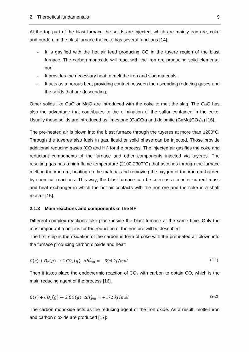
The first step is the oxidation of the carbon in form of coke with the preheated air blown into
the furnace producing carbon dioxide and heat:
𝐶(𝑠) + 𝑂2(𝑔) → 2 𝐶𝑂2(𝑔) ∆𝐻298° = −394 𝑘𝐽/𝑚𝑜𝑙 (2-1)
Then it takes place the endothermic reaction of CO2 with carbon to obtain CO, which is the
main reducing agent of the process [16].
𝐶(𝑠) + 𝐶𝑂2(𝑔) → 2 𝐶𝑂(𝑔) ∆𝐻298° = +172 𝑘𝐽/𝑚𝑜𝑙 (2-2)
The carbon monoxide acts as the reducing agent of the iron oxide. As a result, molten iron
and carbon dioxide are produced [17]:

2. Theroetical fundamentals 10
3 𝐹𝑒2𝑂3(𝑠) + 𝐶𝑂(𝑔) → 2 𝐹𝑒3𝑂4(𝑠) + 𝐶𝑂2(𝑔) 𝑎𝑡 400 − 600°𝐶 (2-3)
𝐹𝑒3𝑂4(𝑠) + 𝐶𝑂(𝑔) → 3 𝐹𝑒𝑂(𝑠) + 𝐶𝑂2(𝑔) 𝑎𝑡 600 − 800°𝐶 (2-4)
𝐹𝑒𝑂(𝑠) + 𝐶𝑂(𝑔) → 𝐹𝑒(𝑠) + 𝐶𝑂2(𝑔) 𝑎𝑡 800 − 1100°𝐶 (2-5)
These reactions take place at different zones of the blast furnace, depending on the
temperature.
2.1.4 Products
The main product of the blast furnace is the pig iron, which is molten iron with a high content
of C (between 4 and 5%) and 0.5-1% of Si. It is extracted from the blast furnace at regular
intervals, or continuously in the case of big blast furnaces, and in a next step it is refined to
obtain steel. The composition of the hot metal produced in the blast furnace is controlled by
the regulation of the temperature of the blast furnace and the slag composition [16].
The process of the blast furnace also produces two by-products:
- Slag: Contains a 30-40% of silicon dioxide (SiO2). The low content of iron oxides
shows an excellent efficiency of the reduction in the blast furnace.
- Blast furnace gas: The flue gas leaves the blast furnace through the top of it. The
typical volume composition of the top gas is, approximately: 23% CO, 22% CO2, 3%
H2, 3% H2O and 49% of N2. The content of CO and H2 gives to this gas a certain
energetic value. Therefore, it can be used as an energy source in other parts of the
steel mill. The heat of combustion of this blast furnace gas is around 4000 kJ/Nm3,
which is about 10 times lower than the combustion heat duty of natural gas [16].
The process of the blast furnace is continually monitored through the measurement of
the composition of the top gas. A good sign of the blast furnace efficiency is the
percentage of CO that has been converted to CO2 during the iron reduction in the
blast furnace:
η𝐶𝑂 =𝐶𝑂2
𝐶𝑂 + 𝐶𝑂2
(2-6)
Through this analysis it can be observed if there is a good relation between the
amounts of reduction gas and iron ore [15].

2. Theroetical fundamentals 11
2.1.5 Integration of the Blast furnace with steam cycle
The process gases produced in the blast furnace have a hot temperature and a high content
of CO/H2. For this reason, they can be used as an energy source for the plant itself or for grid
power production.
The gases come from different sources: the blast furnace itself, producing the called Blast
Furnace Gas (BFG), the coke oven plant and the basic oxygen furnace.
Power plants have an important role in steel mills consuming these gases and providing
steam and power to all key processes during the steel production. Traditionally, the blast
furnace steel plants were integrated with a conventional steam cycle power plant, where the
steam generated from burning the low calorific process gases was expanded in a steam
turbine. Other fuels, such as natural gas or oil, were usually also fed. Recently this plant
layout has been replaced with a more efficient combined cycle [4].
2.2 ULCOS Top Gas Recycling Blast Furnace
The Top Gas Recycling Blast Furnace (TGR-BF) aims at reducing the CO2 emission of the
blast furnace by 50% via the reinjection of the top gas exiting the blast furnace, which
contains unreacted reducing agents (CO and H2). The reinjection of most of the top gas
through the shaft and hearth tuyeres, after CO2 recovery and reheating, lowers the carbon
consumption (coke).
This process requires the operation with oxygen instead of hot blast air to avoid nitrogen
accumulation. To achieve this target in the reduction in the CO2 emission it is not only
necessary the decrease of fossil carbon consumption but also the underground storage of
the separated CO2.
Within the ULCOS project the top gas recycling was tested in LKAB’s Experimental Blast
Furnace (EBF) in Luleå, Sweden. A VPSA (Vacuum Pressurized Swing Adsorption) plant
was used for the CO2 separation of the top gas [7].
Different configurations were tested during this phase of the project changing the point of re-
injection and the temperature of the de-carbonated gas, which varied from room temperature
to 1250°C. In the first two campaigns (2007 and 2009) the versions tested were:
- Version 1: The top gas was injected cold at the hearth tuyeres with pure oxygen and
coal. At the shaft tuyeres the decarbonated gas was injected hot.
- Version 3: The decarbonated top gas was recycled with coal and oxygen hot at the
main tuyeres (hearth) only.
- Version 4: In this version the gas was injected hot in both hearth and shaft tuyeres.

2. Theroetical fundamentals 12
The results of these first experiments of the project showed that the called Version 4 gave
the best results. In this version the hot de-carbonated gas was re-injected in both at blast
tuyeres at 1200°C and in the shaft at 900°C. During the third and last campaign this 4th
version was tested in depth.
A carbon saving of 24% of the total consumption was achieved with a top gas recycling ratio
of 90%. That means that the consumption of coke and coal was reduced in 123 kg/thm
compared to the reference Experimental Blast Furnace. The coke consumption was reduced
approximately in 17 kg/100 Nm3 of top gas recycled (CO+H2) [9].
These campaigns showed that a much lower carbon consumption, and in consequence, CO2
emission, was possible compared to today´s best blast furnaces. In average, the actual
consumption 470 kgC/thm could be lowered to approximately 350 kgC/thm.
Figure 2-4: Flow sheet in Version 4 [18]
This reduction of the carbon input will as a direct consequence have a reduction of the CO2
emissions of, approximately, 24%. However, as it has been explained before, in an
integrated steel mill the top gas of the blast furnace has another use. In the TGR-BF the top
gas will not be available for any other process of the plant, so the energy that this gas was
providing will have to be replaced by natural gas or another source.
Taking into consideration this extra energy, it has been proved that with the utilization of the
CCS technology together with the TGR-BF a decrease of 60% of the CO2 emission in the
steelwork can be achieved [5].

2. Theroetical fundamentals 13
2.3 Alternative post-combustion CO2 capture technologies
2.3.1 VPSA technology
The current CO2 separation technology used in the Experimental Blast Furnace of the
ULCOS project is a physical absorption technology named Vacuum Pressure Swing
Adsoprtion (VPSA).
VPSA is a cyclic process where some components from a multicomponent gas mixture are
selectively retained in a porous material, in this case, zeolite 13X [19]. The process is carried
out by two beds that work in parallel. One of them is adsorbing and the other one is
desorbing at lower pressure. Normally the adsorption of the components (named heavy
components) is carried out at the highest pressure of the system and the desorption, which is
the regeneration, involves the use of vacuum at lower pressure.
The process can be done in a different number of steps, the typical ones are:
- Pressurization of the bed to the feed pressure
- Feed admission into the column, where the CO2 is adsorbed
- Depressurization, where feed is stopped and the pressure in the column is reduced
- Blowdown, where the most adsorbed components are partially removed of the
adsorbent. Here is recovered at the lowest pressure the high-purity CO2
- Purge, where an inert gas is blown counter-current to remove the heavy gas from the
gas phase [19], [20].
2.3.2 MDEA/Piperazine
A method regularly used for CO2 capture is the chemical absorption with amines. MDEA/Pz,
which stands for Methyl-Di-Ethanol Amine activated with Piperazine, is a widely established
sorbent, commercially available (BASF, UOP, Shell, Ineos) and that offers some advantages
over monoethanolamine (MEA), like its resistance to thermal and oxidative degradation at
typical adsorption and stripping conditions, its greater capacity and its lower equivalent work
for CO2 removal.
This method has been used for years in the natural gas industry for the removal of CO2 and
H2S. The process requires two reactors. In the first of them, the absorber, the gas flow rich in
CO2 interacts with the solvent. The purified gas leaves the absorber at the top, whereas the
rich solvent is heated up previous entering the second reactor, which is a desorber column.
In the desorber the regenerated solvent as well as stripped CO2 are obtained.
2. Theroetical fundamentals 14
2.4 Calcium Looping Process
2.4.1 Description of the process
The Calcium Looping cycle is one of the most promising post combustion CO2 capture
processes due to its low cost and energy penalties. The concept was proposed in 1999 by
Shimizu et al. [21] and it is based in the reversible reaction of the CO2 of the flue gases with
calcium oxide:
𝐶𝑂2(𝑔) + 𝐶𝑎𝑂(𝑠) ↔ 𝐶𝑎𝐶𝑂3(𝑠) (2-7)
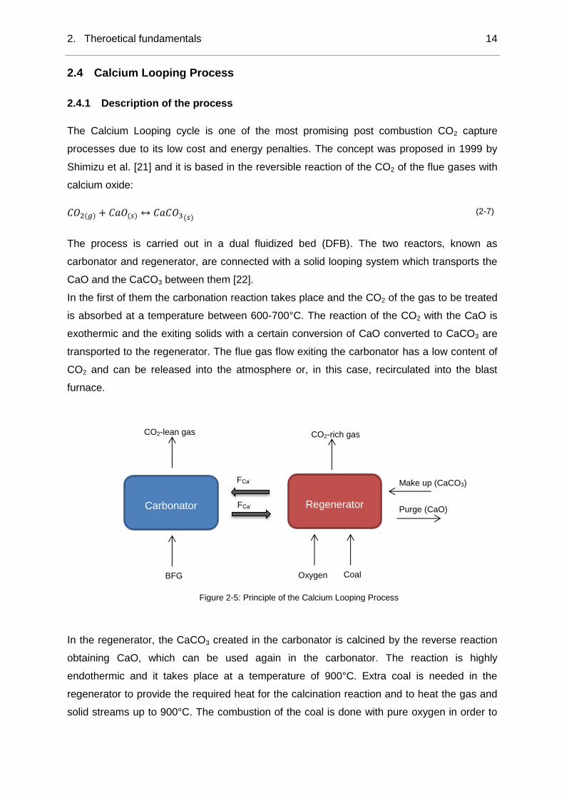
The process is carried out in a dual fluidized bed (DFB). The two reactors, known as
carbonator and regenerator, are connected with a solid looping system which transports the
CaO and the CaCO3 between them [22].
In the first of them the carbonation reaction takes place and the CO2 of the gas to be treated
is absorbed at a temperature between 600-700°C. The reaction of the CO2 with the CaO is
exothermic and the exiting solids with a certain conversion of CaO converted to CaCO3 are
transported to the regenerator. The flue gas flow exiting the carbonator has a low content of
CO2 and can be released into the atmosphere or, in this case, recirculated into the blast
furnace.
In the regenerator, the CaCO3 created in the carbonator is calcined by the reverse reaction
obtaining CaO, which can be used again in the carbonator. The reaction is highly
endothermic and it takes place at a temperature of 900°C. Extra coal is needed in the
regenerator to provide the required heat for the calcination reaction and to heat the gas and
solid streams up to 900°C. The combustion of the coal is done with pure oxygen in order to
CO2-lean gas CO2-rich gas
Purge (CaO)
Make up (CaCO3)
FCa‘
Xcarb
Carbonator Regenerator
FCa‘
Xcalc
Oxygen Coal BFG
Figure 2-5: Principle of the Calcium Looping Process

2. Theroetical fundamentals 15
avoid the contamination of nitrogen of captured CO2 stream. The hot CO2-rich gas exiting the
regenerator has a high purity and can be directly processed and sent to storage.
In addition, a make-up flow of sorbent has to be injected in the regenerator to neutralize the
sorbent deactivation through multiple cycles [23], [24].
Fluidized bed reactors are utilized for the CaL process because of the high reaction rate
required and the high enthalpies of the reactions. Another advantage is the fact that fluidized
bed are a mature and developed technology [22].
Calcium Looping has been tested in different facilities at pilot scale [25], [26] and in pilot
plants [27] with realistic process conditions and the results reported a high CO2 capture
efficiency (>90%) [23].
Besides the high efficiency, one of the main advantages offered by the process is the low
price and high availability of the material used in the cycle, natural limestone. Furthermore,
as it is a post-combustion process, its utilization in existing fossil fuel power plants or, in the
case of this project, existing blast furnaces is possible without many additional modifications.
2.4.2 The calcium oxide-carbon dioxide equilibrium
The extent of the reaction between CaO and CO2, therefore the operation of the CaL
process, can be predicted from the thermodynamic equilibrium theory [28]. The CO2 partial
pressure of equilibrium has been experimentally determined by different authors [29]. In the
study [30], three expressions of the decomposition pressure of carbon dioxide over calcium
carbonate are summarized and plotted.
Figure 2-6: Equilibrium equations of the decomposition of CO2 [30]

2. Theroetical fundamentals 16
Temperatures and pressures above and to the left of the equilibrium line will favour the
carbonate formation. Thus if there is sufficient CaO to capture CO2 and sufficient time, CaO
will react with CO2. For temperatures below and to the right of equilibrium the carbonate
decomposition will be favoured [28], [31].
It can be seen then, that for a temperature of 650°C the equilibrium partial pressure is around
0.01 atm. Thus, high separation efficiency can be achieved when a flue gas with a typical
content of 15% of CO2 reacts at this temperature with CaO [28].
2.4.3 Energy recovery
A large amount of energy is introduced into the system to heat the gas and solid streams up
to the regenerator temperature and to provide the necessary heat for the endothermic
reaction. Nevertheless, unlike in other CO2 capture methods, Calcium Looping enables the
recovery of part of this heat [32].
The flue gases leaving the carbonator and the regenerator are at 650 and 900°C respectively
and also extra energy can be recovered in the carbonator due to the heat produced in the
exothermic carbonation reaction [33], [34].
Thus, if Calcium Looping is applied to a power plant or to a blast furnace with steam
generation, it is possible to increase the total amount of electricity or steam generated
reducing then the energy penalty of the capture process.
When the Calcium Looping process is utilized as a post-combustion capture system in coal-
fired power plants the heat steam generation is enhanced by the recovery of energy from the
3 sources: CO2-lean gas leaving the carbonator, CO2-rich gas leaving the regenerator and
heat generated in the carbonator, i.e. 168 kJ/mol from the carbonation reaction.
However, in the application of the process at the TGR-BF the heat can only be recovered
from two sources, because the CO2-lean gas leaving the carbonator at 650°C is recycled into
the blast furnace at even higher temperatures.
2.4.4 Characteristics of the CaL process
A useful parameter for the measurement of the process efficiency is the carbon dioxide
capture efficiency, ECO2, which is defined like:
𝐸𝐶𝑂2 = 1 −𝐹𝐶𝑂2𝑜𝑢𝑡
𝐹𝐶𝑂2𝑖𝑛 (2-8)
During the compression of the separated CO2-rich flow, part of the CO2 is lost and emitted to
the atmosphere. This CO2-slip stream represents approximately 5% of the stream leaving the
regenerator. Therefore the carbon dioxide capture efficiency should be changed to:

2. Theroetical fundamentals 17
𝐸𝐶𝑂2 = 1 − (𝐹𝐶𝑂2𝑜𝑢𝑡 + 𝐹𝐶𝑂2𝑠𝑙𝑖𝑝,𝑠𝑡𝑟𝑒𝑎𝑚
𝐹𝐶𝑂2𝑖𝑛)
( 2-9)
Where 𝐹𝐶𝑂2𝑠𝑙𝑖𝑝,𝑠𝑡𝑟𝑒𝑎𝑚 represents the loss of CO2 during compression. This loss of CO2 will not
be taken into account in the calculation of the project to compare under the same conditions
the CaL with other capture technologies where this loss was not considered either.
If a molar balance in the carbonator is made, the following equation is obtained [26]:
𝐸𝐶𝑂2∙ 𝐹𝐶𝑂2
= 𝐹𝐶𝑎𝑂(𝑋𝑐𝑎𝑟𝑏 − 𝑋𝑐𝑎𝑙𝑐) (2-10)
Where Xcarb is the fraction of CaO converted to CaCO3 after leaving the carbonator, FCaO is
the molar flow that enters the carbonator and FCO2 is the molar flow of CO2 introduced into
the carbonator for being treated. Xcarb makes reference to the fraction of carbonate in the
sorbent after leaving the regenerator, and assuming full conversion, can be considered equal
to zero. Thus, the carbon capture efficiency can be also expressed as:
𝐸𝐶𝑂2=
𝐹𝐶𝑎𝑂 ∙ 𝑋𝑐𝑎𝑟𝑏
𝐹𝐶𝑂2
(2-11)
Through experimental investigations the influence of diverse parameters on the CO2 capture
efficiency has been studied [25], [27].
The Calcium Looping ratio (LR) is defined as the relation between the molar flow of
circulating CaO from the regenerator to the carbonator (FCaO) and the molar flow of CO2
entering the carbonator (FCO2) (2-12). Another related characteristic parameter is the space
time (𝜏) that is defined as the ratio of moles CaO (nCa) present in the carbonator and the flow
of CO2 entering in it (2-13):
𝐿𝑅 =𝐹𝐶𝑎𝑂
𝐹𝐶𝑂2
(2-12)
𝜏 =𝑛𝐶𝑎
𝐹𝐶𝑂2
(2-13)
One useful parameter presented by Abanades et al. [35] is the free active CaO, fa, which is
defined as the free active CaO fraction available for reaction with CO2. If Xsulf is defined as
the fraction of active CaO that has reacted with sulfur producing CaSO4, the maximum
conversion of an average CaO particle (Xmax) can be expressed as [25], [27]:

2. Theroetical fundamentals 18
𝑋𝑚𝑎𝑥 = 𝑋𝑐𝑎𝑟𝑏 + 𝑋𝑠𝑢𝑙𝑓 + 𝑓𝑎 (2-14)
The reactivity of the sorbent particles decays with the number of cycles. For maintaining the
capture efficiency a fresh make-up is required. The principal causes for the decrease of the
capture capacity of the particles are presented in section 2.4.6.
As an evaluation of the amount of make-up introduced in the regenerator, the make-up ratio
is defined. This characteristic parameter is defined as the molar ratio of fresh limestone
introduced in the reactor divided by the molar flow of CO2 treated in the carbonator.
𝑀𝑎𝑘𝑒 − 𝑢𝑝 𝑟𝑎𝑡𝑖𝑜 =𝐹𝐶𝑎𝐶𝑂3
𝐹𝐶𝑂2
(2-15)
2.4.5 Adsorption-Enhanced Reforming
Besides the application of post-combustion CO2 capture technology, Ca-Looping can be
used as a pre-combustion capture technology. This is the case of Adsorption-Enhanced
Reforming (AER). This technology is based on the capture of the CO2 in-situ in the steam
gasifier in order to enhance the water-gas shift reaction, increasing the hydrogen production
[27], [29]:
𝐶𝑂(𝑔) + 𝐻2𝑂(𝑔) ↔ 𝐻2(𝑔) + 𝐶𝑂2(𝑔) ∆𝐻 = −40,9 𝑘𝐽/𝑚𝑜𝑙 (2-16)
The operation of the AER is similar to the one of the CaL cycle described before. The CaCO3
used as a bed material in the DFB biomass gasification process has a double function: heat
carrier and selective CO2 transport from the gasification reactor to the combustion reactor
[36].
In this study, the Blast Furnace Gas that is treated has a high content of CO but does not
have water. Thus, if steam were introduced in the carbonator fluidized bed reactor (or
gasifier) the water-gas shift reaction could take place producing a gas with a high content of
hydrogen.
This case is similar then to a CO2 capture to increase the H2 production after the gasification
step, as proposed by Armbrust [37], with the difference that the gas comes from a blast
furnace instead of being the syngas derived from a biomass gasification.
2.4.6 Reactivity of the CaO particles
The stoichiometric CO2 capture efficiency of a CaO particle is 78.6 wt-%. [38]. However, it
has been experimentally observed that the carrying capacity of the particles decreases
rapidly in the first 20 cycles to a residual value [26], [39].

2. Theroetical fundamentals 19
It is well known that the decay in the reactivity of the sorbent through multiple CO2 capture
and release cycles affects the cost and efficiency of the process. This sorbent reactivity
decay is associated to different factors including sintering, attrition and reaction with
impurities with the flue- or fuel gas, especially sulfur species such as SO2 or H2S [39].
The sintering of small CaO grains towards larger grains reduces the free surface of CaO,
affecting the rate of carbonation [38]. Sintered particles have lower porosity, which is
characterized by a reduced number of large pores, whereas fresh particles have a high
porosity due to a large number of small pores [29], [40].
Another parameter that affects the reactivity of the sorbent is the content of sulfur. The sulfur
particles disable the sorbent capture potential reacting with the CaO and reducing the
amount of CaO available for CO2 capture. This can be substantial in gasification of coal
(containing S) or in post-combustion CO2 capture process without previous desulfuration.
The study [22] describes this behaviour with two reactions taking place in the carbonator and
in the regenerator:
𝐶𝑎𝑂 + 𝑆𝑂2 + 1
2𝑂2 → 𝐶𝑎𝑆𝑂4 ∆H = −501 kJ
(2-17)
𝐶𝑎𝐶𝑂3 + 𝑆𝑂2 + 1
2𝑂2 → 𝐶𝑎𝑆𝑂4 + 𝐶𝑂2 ∆H = −323 kJ
(2-18)
Reaction (2-17) is irreversible in the temperature range of request so the sorbent reacted
with the sulfur is permanently lost [41]. The direct result of the SO2 capture in the cycle is a
higher make-up consumption.
Regarding to the loss of solids by attrition, several studies in this topic have been carried out
and different mechanisms of attrition and fragmentation are detailed elsewhere [41]–[44].
Limes has a high porosity and a relative fragility and may attrite higher than other materials
generally utilized in fluidized beds [23]. The consequence of this phenomenon is an increase
of the number of particle and a decrease of its size. The characteristics of the reactor,
particle velocity and exposure time have been proven to play an important role in the attrition
rate [42].
The deactivation is also associated to the formation of a product layer surrounding the CaO
particle, which, after a certain reached thickness, impedes the carbonization of the inner
parts of the particle [45].
Although the particles keep a residual carrying capacity of around 7.5 mol-%, this value is not
enough to capture the inlet amount of CO2 [24]. For this reason, a continuous make-up of
2. Theroetical fundamentals 20
solids is needed [23]. This make-up could be introduced as CaO in the carbonator or CaCO3
in the regenerator but obviously, due to its cheaper prize and high abundance, the make-up
is introduced as natural limestone directly into the regenerator. Another characteristic that
gives to this process an advantage is that the purge of deactivated CaO can be utilized in
other processes, like the cement industry. In the proposed case the CaO may be used
directly in the blast furnace itself, which, as it has been said before in 2.1.2 needs CaO for
the sulfur elimination and slag melting.
2.5 Other processes
2.5.1 Air Separation Unit
The combustion in the calciner is carried out in an O2/CO2 atmosphere, avoiding the
presence of nitrogen in order to obtain a flue gas of pure CO2 directly available for
compression and storage. However, the combustion with only oxygen would produce too
high temperatures (nearly 3500°C). For this reason part of the CO2 is redirected to the
regenerator at a lower temperature after heating other streams, decreasing the temperature
in the combustor reactor without affecting the CO2 purity.
The oxygen required is produced in an Air Separation Unit (ASU) that separates the air in its
elemental components: oxygen, nitrogen and argon. The ASU produces an oxygen-rich
stream of about 95% of oxygen, being the rest argon and nitrogen. Liquid argon, present in
the air in a 0.93%, is obtained also as a by-product and can be sold at a prize of 0.9299
US$/Nm³, which can represent a substantial benefit in a real steel mill [12].
The ASU is based on the principle of the cryogenic distillation. The condensation points of
the oxygen and the nitrogen are -183°C and -195.8°C, respectively. The air is compressed in
four stages with interstage cooling. During the compression condensed water is extracted
from the air and the compressed air is passed through an integrated heat exchanger. An
expansion turbine expands part of the processed air for further cooling to a temperature of -
175°C and 2 bar. Part of the air liquefies in a low-pressure distillation column (2 bar) to form
a liquid that is enriched in oxygen. The nitrogen-rich vapour is further purified in the high
pressure column (6 bar) [38],[39].
The oxygen produced has an additional function. As it has been explained before, in the
TGR-BF the coke is combusted with oxygen instead of air, so there are two main oxygen
consumers: the blast furnace itself and the regenerator.
A regular reference steel mill requires also a certain amount of high-purity oxygen (99%),
approximately 121.4 Nm³/t HRC. This oxygen is consumed basically in the steelmaking
process and, to a lower extent, in the iron making process. A steel mill operating with an

2. Theroetical fundamentals 21
Oxygen Blast Furnace and Top Gas Recycling requires higher amount of oxygen but the
purity necessary is lower (95%). Although, as a result of reducing the high-purity oxygen
produced, the sales of liquid argon are also reduced [12].
In the following table is represented the energy requirements of the ASU for the production of
high and low purity oxygen in the reference steel mill and the TGR-BF steel mill proposed by
[12]:
Table 2-2: Oxygen requirements in the steel mill [IEA]
Electricity
consumption
ASU
Steam
consumption
ASU
Reference steel
mill O2
consumption
Steel mill with
TGR-BF O2
consumption
High Purity O2 0.48 kWh/Nm³ 0.06 kg/Nm³ 121.4 Nm³/t HRC 69.1 Nm³/t HRC
Low purity O2 0.33 kWh/Nm³ 0.02 kg/Nm³ - 256.1 Nm³/t HRC
Steam is required in the ASU for product re-gasification and TSA regeneration. Electricity is
required for the air and product compressors and for the cooling water pumps.
The oxygen consumption in the TGR-BF steel mill is increased by 170%, reaching 325.1
Nm3/t HRC. This increment is due to the use of oxygen in the Top Gas Recycling Blast
Furnace which consumes about 5 times more oxygen than a conventional one.
2.5.2 CO2 conditioning and storage
The CO2-rich gas obtained is cleaned of impurities and pressurized to 110 bara for its
transportation and geological storage.
The CO2 compression unit consists of five compressors with intercoolers. The temperature
can be reduced with feed water to 50°C. Thus, external cooling water at 13°C is required to
reduce the gas the temperature to 25°C. After four stages, the CO3 at 75 bar is liquefied.
Then the liquid stream is compressed until 110 bar by a gear pump that consumes much less
power than a compressor.
As it has been commented, during the compression process a CO2-slip stream is inevitably
lost. This loss has not been considered in the calculation of CO2 emissions of the CaL steel
mill for an easier comparison with the other CO2 capture technologies (MDEA and VPSA)
where the loss had not been considered by other authors either.

2. Theroetical fundamentals 22
2.6 Fundamentals of the economic analysis
The economic feasibility of the CaL process will be studied in chapters 6 and 7. In a first step
the framework conditions for the economics analysis will be defined.
2.6.1 Price basis
For the calculation of the capital costs of the CaL, as a basis it will be taken the Euro [€] at
the year 2004. This year has been chosen to use the same price basis as other studies
where power plants with CO2 capture were studied [48], [49]. For the comparison with the
results of the International Energy Agency (IEA) study [12], where the TGR-BF along
MDEA/Pz capture is analyzed, the same basis price will have to be used, which was [$] at
the year 2010.
Therefore, a conversion of the costs in [€] to [US$] will be carried out with the average rate of
2004 (US$ 1.2199 = 1€). Afterwards, the inflation and material price increase are considered
and the costs are actualized to the year 2010 using the Chemical Engineering Plant Cost
Index (CEPCI), included in Appendix 9. When the conversion of [€2010] to [US$2010] is
necessary the average ratio of 2010 is considered (US$ 1.3268 = 1€). In addition, the
conversion of [A$] to [€] at year 2010 has been considered A$1=0.6933€.
The inflation has not been assumed during the lifetime of the plant.
2.6.2 Interest rate
For the calculation of the investment cost of the CaL plant it has to be considered that the
financing can be carried out with different sources. The real interest is calculated taking into
account the cost of the own and external capital. In this case both interests are considered
equal to an 8%.
𝑖𝑟 =𝐼𝐶 ∙ 𝑖𝐼𝐶 + 𝐸𝐶 ∙ 𝑖𝐸𝐶
𝐼𝐶 + 𝐸𝐶
(2-19)
𝐼𝐶: Fraction of internal capital (%),
𝐸𝐶: Fraction of external capital (%),
𝑖𝐼𝐶: Interest of the internal capital (%),
𝑖𝐸𝐶: Interest of the external capital (%),
2.6.3 Plant life and construction period
The CaL CO2 capture plant is assumed to have an economic life of 25 years, which is the
same economic life as the integrated steel mill.

2. Theroetical fundamentals 23
It is assumed that the construction of the plant will last 4 years. The capital expenditure
during the construction is considered the following:
- Year 1: 15%
- Year 2: 30%
- Year 3: 35%
- Year 4: 20%
2.6.4 Capital costs
Capital costs are the costs of bringing the project of the Calcium Looping plant to an
operating status, including the total investment costs and the financing costs. The capital
costs during the planning horizon can be calculated through the following expression:
𝐶𝐶𝑛 = 𝐴𝑀 + 𝐼𝑃𝑛 (2-20)
Where :
- 𝐴𝑀: Amortization (€/y)
𝐴𝑀 =𝐼𝑡𝑜𝑡
𝑛𝐿
(2-21)
𝐼𝑡𝑜𝑡: Total investment costs (€)
𝑛𝐿: Useful life of asset (years)
- 𝐼𝑃𝑛: Interest payment (€/y), which during the years will decrease because the
remaining investment costs to pay will be lower.
𝐼𝑃𝑛 = [𝐼𝑡𝑜𝑡 − (𝑛 − 1) ∙ 𝐴𝑀] ∙ 𝑖𝑟 (2-22)
𝑛: Calculation year
𝑖𝑟: Real interest (%)
The total investment costs (Itot) are defined as:
𝐼𝑡𝑜𝑡 = 𝐶𝑖𝑛𝑠 + 𝐶𝑐𝑜𝑛𝑠 + 𝐼𝐷𝐶 (2-23)
Where:
- 𝐶𝑖𝑛𝑠: Total cost of the installation
- 𝐶𝑐𝑜𝑛𝑠: Personal contribution by the building owners. This cost is assumed to be a 15%
of the total cost of the installation (𝐶𝑖𝑛𝑠).
- 𝐼𝐷𝐶: Interest generated during the planning period and the construction of the
installation. It is calculated with the installation cost including the personal contribution
by the building owners.

2. Theroetical fundamentals 24
𝐼𝐷𝐶 = ∑ (𝑍1 + ⋯ + 𝑍𝑛)𝑛𝑖=1 (2-24)
𝑍𝑛 = 𝐶𝑖𝑛𝑠 ∙ (𝑛. 𝑎𝑙𝑙𝑜𝑐𝑎𝑡𝑖𝑜𝑛) ∙ (1 +𝑖𝑐
100)
(𝑘−𝑛)
(2-25)
𝑛. 𝑎𝑙𝑙𝑜𝑐𝑎𝑡𝑖𝑜𝑛: Fraction of the construction costs in year n [%]
𝑛: Year of calculation
𝑘: Period of construction (4 years)
𝑖𝑐: Interest during the construction and planning period [%]
For the calculation of the investment costs of the equipment reference literature data will be
used as a basis. The cost and the size of a unit will be mathematically related with the
function:
𝐶 = 𝑎 ∙ 𝑃𝑚 (2-26)
Where 𝐶 symbolizes the investment cost of the unit expressed in [€], 𝑃 represents the size or
power of the unit, 𝑎 is a costs constant and 𝑚 makes reference to decreasing cost factor,
which takes into account the economy of scale of the units.
This cost estimation method is based on power law expression and was proposed by
Williams R. (1947). It is commonly known as rule of six-tenths, because m=0.6 is a widely
used factor.
𝐶
𝐶0= (
𝑃
𝑃0)
𝑚
(2-27)
From this expression the value of m can be deduced when data from two or more
comparable units are available:
𝑚 =log (
𝐶𝐶0
)
log (𝑃𝑃0
)
(2-28)
2.6.5 Operating costs
The operating costs of the CaL are all the costs generated during the operation except the
fuel and limestone costs. They are composed from fix and variable costs. Fix operating costs
(OCfix) include:
- Personal costs
- Maintenance and reparation costs
- Insurance costs
2. Theroetical fundamentals 25
Variable operating costs depend on the amount of CO2 treated in the CaL process.
Although the fuel and the limestone costs are part of the operational costs, they will be
separately calculated because of its significance in relation to the total costs.
2.6.6 Cost of steel production
The costs of steel production are calculated by addition of the O&M costs of the steel mill to
the annualized cost of capital of the entire steel mill, including the costs of the CO2 capture
plant. The capital costs are annualized using the capital recovery factor, for the defined
operational period and interest.
Capital recovery factor:
𝐶𝑅𝐹 =𝑖𝑟 ∙ (1 + 𝑖𝑟)𝑛
(1 + 𝑖𝑟)𝑛 − 1
(2-29)
Where 𝑛 is the project life (25 years) and 𝑖𝑟 is the nominal interest rate (10%).
The cost of transportation and geological sequestration of the CO2 is not regarded. The cost
of emission of CO2 and the decommissioning and demolition costs are not considered either.
Thus, the present value of total costs (PVTC) of the steel mill is calculated as:
𝑃𝑉𝑇𝐶 = ∑𝐶𝐶𝑛
(1 + 𝑖𝑟)𝑛+ ∑
𝐹𝑢𝑒𝑙&𝑟𝑒𝑑𝑢𝑐𝑡𝑎𝑛𝑡 𝐶𝑛
(1 + 𝑖𝑟)𝑛+ ⋯ + ∑
𝑀𝑖𝑠𝑐. 𝐶𝑛
(1 + 𝑖𝑟)𝑛
(2-30)
Where 𝐶𝐶𝑛 are the total capital costs of steel mill at year 𝑛, including the investment costs of
the CO2 capture plant. Then, all the operating costs of the steel mill are added as it is shown
for the fuel and reductant costs. These costs are presented in section 7.2 and are, for the
reference steel mill:
- Fuel & reductant costs
- Iron ore costs
- Scrap & ferroalloys costs
- Fluxes of the steel mill (Limestone, Quartzite, Olivine, Calcium Carbide)
- Consumables & other utilities
- Labour costs
- Maintenance costs
- Miscellaneous costs
For the steel mill with TGR-BF and CaL the operating costs of the CaL plant are added
together with the fuel and limestone costs of the CaL to the equation (2-30).
2. Theroetical fundamentals 26
Once the present value of the total costs of the steel mill is calculated, the cost is annualized,
obtaining the levelized total annual costs (𝐿𝐴𝑁).
𝐿𝐴𝑁 = 𝑃𝑉𝑇𝐶 ∙ 𝐶𝑅𝐹 (2-31)
With this value and knowing the annual production of steel (hot rolled coil in this case), the
cost of steel production can be calculated as:
𝐶𝑆𝑡𝑒𝑒𝑙 𝑃𝑟𝑜𝑑𝑢𝑐𝑡𝑖𝑜𝑛 =𝐿𝐴𝑁
𝐴𝑛𝑛𝑢𝑎𝑙 𝑡 𝐻𝑅𝐶 [
$
𝑡 𝐻𝑅𝐶]
(2-32)
Once the cost of steel production is calculated, the cost of capture in the steel mill can be
estimated. The costs of steel production are calculated for the reference steel mill and the
steel mills with CO2 capture (MDEA, VPSA and CaL). Then, the cost of capture can be
calculated as the increase of the cost of steel production divided by the CO2 avoided in the
production of this steel.
𝐶𝑜𝑠𝑡 𝐶𝑂2 =𝐶𝑜𝑠𝑡 𝑜𝑓 𝑝𝑟𝑜𝑑𝑢𝑐𝑡𝑖𝑜𝑛𝐶𝑎𝑝𝑡𝑢𝑟𝑒 𝑆𝑀 − 𝐶𝑜𝑠𝑡 𝑜𝑓 𝑝𝑟𝑜𝑑𝑢𝑐𝑡𝑖𝑜𝑛𝑅𝑒𝑓𝑆𝑀
𝐶𝑂2 𝐸𝑚𝑅𝑒𝑓𝑆𝑀 − 𝐶𝑂2 𝐸𝑚𝐶𝑎𝑝𝑡𝑢𝑟𝑒 𝑆𝑀
(2-33)

3. Simulation of the CaL process 27
3 Simulation of the CaL process
3.1 Aspen PlusTM Simulator
The software Aspen PlusTM will be used for the study of the CaL process applied to the
treatment of blast furnace gas and its preparation before the re-injection into the blast
furnace.
Aspen PlusTM is a widely used process simulator that enables the calculation of material and
energy streams. The software has integrated the most important unit operations of the
chemical industry and can be used to simulate them in a steady state, obtaining the flow
rates, compositions, properties and operation conditions.
These units operations and its energy and material streams are drawn and defined in the
flowsheet. Aspen PlusTM includes a large thermodynamic database and through energy and
material balances and phase and chemical equilibrium the desired system can be simulated.
3.1.1 Reactor models in Aspen PlusTM
Aspen PlusTM offers different models of reactors based on different operating principles. The
kind of reactor chosen for the carbonator and regenerator simulation will affect the final
results. For this kind of purpose, where the kinetics are not important and there is a
reversible reaction the RGIBBS- and the RSTOIC-Reactors can be chosen.
RGIBBS is a reactor based on the Gibbs free energy minimization. It calculates the single
phase chemical equilibrium or simultaneous phase and chemical equilibria. In this reactor it
is not necessary to define either the chemical reaction or the stoichiometry. Additionally, it is
possible also to restrict the equilibrium to adjust the simulation to experimental data.
In RSTOIC the kinetics are also unimportant but the stoichiometry of the reaction has to be
defined by the user, allowing the specification of an extent of reaction [50].
The property method used in the simulation is the Peng-Robinson cubic equation of state
with the Boston-Mathias alpha function. This property method is recommended for gas-
processing, refinery and petrochemical applications. The obtained results have been also
compared to the RK-Soave property method and both are in agreement.
3.1.2 Coal definition
For the combustion in the regenerator the bituminous coal “Douglas Premium” has been
selected. The coal combusted in the regenerator is defined as a non-conventional
component. These components are basically components whose molecular-weight is

3. Simulation of the CaL process 28
unknown and that are not participating in the chemical equilibrium. The heat of combustion of
the coal is introduced as an input. In this case the low heating value is 27214.2 kJ/kg.
The stream “COAL” is specified as a non-conventional stream. The models HCOALGEN and
DCOALIGT of Aspen PlusTM will calculate the enthalpy and the density of the coal. Three
categories are required as an input to calculate the enthalpy of the coal: proximate analysis
(PROXANAL), ultimate analysis (ULTANAL) and sulfur analysis (SULFANAL). In Table 3-1
and Table 3-2 proximate and ultimate analysis of Douglas Premium coal are presented.
Sulfur analysis describes the type of sulfur of the coal. For this bituminous coal it has been
considered that the sulfur is in a 45% pyritic, 45% organic and 10% sulfate.
Table 3-1: Proximate analysis
Constituents Moisture Fixed carbon (FC) Volatiles (VM) Ash
% weight 8 54.9 22.95 14.15
% weight, dry - 59.67 24.95 15.38
Table 3-2: Ultimate analysis
Constituents Ash C H N Cl S O
% weight 15.38 72.3 4.11 1.7 0 0.58 5.93
3.2 Basic simulation without heat integration
In a first step of the project a basic Calcium Looping model without heat integration has been
simulated. The blast furnace gas enters into the carbonator, which has been simulated with
the RGibbs reactor, and a certain amount of CO2 is captured. In this first step it has been
considered that the equilibrium is reached. Although it has been experimentally seen that the
conversion is really high (>90%), the equilibrium is a too optimistic situation for inlet gases
without any water, as in the present case. The study [39] examined the influence of the
presence of steam during carbonation and concluded that it reduces the diffusion resistance
during carbonation, improving the carrying capacity of the particles. For this reason, since in
this case there is no water in the gas, the block used for the carbonator simulation will be
changed in a future step to stoichiometric reactor to obtain more realistic capture results than
the equilibrium.

3. Simulation of the CaL process 29
3.2.1 General assumptions
There are some general assumptions that have been done in order to simulate the Calcium
Looping process treating the gas of the TGR-BF.
First of all, Aspen PlusTM works with continuous flows and its calculations are in steady state.
For this reason the amount of gas emitted per ton of hot metal produced in the blast furnace
has been converted to a flow. In the simulation it has been considered that the production of
one ton of hot metal lasts one hour. Therefore the gas emitted per ton of hot metal produced
has been introduced in Aspen as a flow per hour. This assumption has been done for having
easier calculations when the scaling of the simulation to the size of a real steel mill is done. It
will not have any impact on the final results, but it will be important to understand when
analysing the final results, that the energy produced in one hour or the moles emitted per
hour equal to the a energy or mass per ton of hot metal.
Regarding the composition of the top gas from the blast furnace that enters into the process,
another assumption has to be done. This is a continuous process where the treated flue gas
is reinjected into the blast furnace, affecting to the composition of the flue gas ejected until a
steady state is achieved. In the simulation, the composition of the gas introduced into the
CaL plant has been taken from the ULCOS TGR-BF [18], where the compositions in a steady
state using VPSA separation are given. This composition has a much lower content of
nitrogen than a regular blast furnace because the blast furnace operates with oxygen instead
of air.
Table 3-3: Composition of the inlet Blast Furnace Gas [17]
Component [vol%]
CO 48%
CO2 38%
H2 8%
N2 6%
The temperature and the amount of ejected gas per ton of hot metal that have been used are
also the same as the most promising version of the ULCOS project (Version 4). Thus, the
BFG in the simulation has a temperature of 110°C, a pressure of 1 atm and a flow is equal to
52.64 kmol/thm (or kmol/h in the simulation).

3. Simulation of the CaL process 30
Other general assumptions considered in the simulation are summarized in Table 3-4:
Table 3-4: General assumptions of the simulation
Assumption Value
Gas dryer efficiency 99% water separation
Ash separation 50% of the ash deducted as bottom-ashes
Cyclone efficiency 100% solid separation
Make-up ratio, F0, (FCaCO3/FCO2) 0.033
Looping molar ratio (FCaO/FCO2) 7
Efficiency of the combustion 3% O2 in the flue gas
Regeneration in the calciner 100% CaO
3.2.2 Description of the basic CaL model
In a first step a basic Calcium Looping cycle has been simulated. In this model, the BFG
leaving the blast furnace enters into the carbonator, where the CO2 is absorbed.
CARBONATOR
T=650°C
REGENERATOR
T=900°C
CaCO3, CaO
CaO
O2, T=20°C
CoalMake-up CaCO3
Ash, purge solids
CO2 to storage
CO2 -lean flue gas
(Processed gas)
Blast Furnace Gas
C O 4 8 , 0 0 %
C O 2 3 8 , 0 0 %
H 2 8 , 0 0 %
N 2 6 , 0 0 %
T e m p . 1 1 0 ° C
1 1 7 9 N m 3 / h
Figure 3-1: Flow diagram of the basic CaL process
Figure 3-3 shows the flowsheet of the basic simulation. The stream “BFG” is defined as a
mixed stream with the composition detailed in Table 3-4 that enters into the block
“CARBONAT”. This block represents the carbonator and in it also enters the stream “TO-
LOOP”, which is defined as the active CaO leaving the regenerator. In a first step the
carbonator has been simulated with a RGibbs reactor. As it has been explained previously,
this reactor is based on the free Gibbs energy minimization to reach the equilibrium. The
temperature and the pressure of the reactor are set to 650°C and 1 atm.

3. Simulation of the CaL process 31
In the reactor the carbon capture takes place and a fraction of the active CaO is converted to
CaCO3. If an equilibrium restriction is not set the reaction will reach the equilibrium.
Therefore, the stream “EXIT” that leaves the block “CARBONAT” is a mixture of solids (CaO
unreacted and CaCO3 converted) and a gas with a lower content of CO2.
The stream is directed to the block “CYCLONE1” that separates the gas and solids
components of the “EXIT” stream with an efficiency of 100%. The solids are represented
with the stream “SOLIDS1” and the gas with “LEAN-CO2”. The solids are conducted then to
the regenerator, represented with the block “REGENER”.
Once the coal is defined as it has been explained in chapter 3.1.2, the stream of coal is
directed to the “DECOMP” block where the coal is decomposed into its constituent elements
(H2, O2, N2, H2O, S, C and ash). This process is represented with the block RYield. The
decomposition reactor does not represent a real process in the combustion but is used as a
tool to convert the non-conventional stream into true components and ash. For this reason, it
is necessary to connect this reactor and the reactor where the coal is burned (“REGENER”)
with a heat stream in order to take into account the energy required for the decomposition.
[51].
Besides the coal, other streams are entering into the regenerator. “CACO3” makes reference
to the make-up introduced as calcium carbonate (CaCO3). This amount of make-up
introduced is calculated as a design specification. The “CACO3” stream is iterated until the
circulating CaO (“TO-LOOP”) is equal to the amount desired (setting the value to meet the
CaO/CO2 ratio) resulting in a molar make-up flow equal to the purge of circulating material.
“OXYGEN” represents the oxygen produced in the Air Separation Unit burned in the
regenerator. This stream is also iterated as a design specification until the flue gas exiting
the regenerator “COMBOUT” has a composition of 3% of O2.
“REGENER” is modelled with the RStoic block and in it the coal is combusted with the
oxygen, providing the necessary heat for the regeneration reaction that also takes place in it.
Thus, the calcination reaction (2-7) is introduced in the RStoic block. The extent of reaction is
defined as a 100% of regeneration, so all the CaCO3 is regenerated into CaO. The
temperature and the pressure of the reactor are set to 900°C and 1 atm respectively, defined
as optimal conditions in previous literature data.
The regenerator is an ideal adiabatic reactor. For simulating this, a heat flow exiting the
regenerator is drawn and iterated to zero through the variation of the flow of coal. Therefore,
the amount of coal introduced into the regenerator is calculated and will be one of the main
outputs of the simulation.

3. Simulation of the CaL process 32
The outlet stream of the regenerator “COMBOUT” contains CaO regenerated, ash and a
CO2-rich gas. The stream is directed to “CYCLONE”, which separates the gas and solids
flows. The gas flow, “HIGH-CO2” has a high content of CO2, water generated in the
combustion and some unreacted oxygen due to its excess in the combustion. The water is
separated in the gas dryer simulated with the block “H2OSEP” with a 99% of efficiency,
resulting two streams: “H2O” and “HIGH-DRY”.
The solid flow exiting “CYCLONE” is named “SOLIDS2” and contains the CaO regenerated
and ash that is separated in a 50% as bottom-ashes at the separator block “BOTTOM”. The
“CAO” stream, after the separation of part of the ash, is transferred into the SSplit block
“PURGE”. There, the loss of circulating material due to attrition is represented. The loss of
circulating CaO has been introduced to match the desired make-up ratio, presented in Table
3-4, which has been achieved in previous experimental studies. This loss of sorbent exits the
system through the stream “PURGE”. Finally, the stream “TO-LOOP” with the regenerated
CaO is directed again to the carbonator reactor.
3.2.3 RStoic carbonator
Afterwards, a less favourable situation will be proposed. Instead of considering the
carbonator as an equilibrium reactor (RGibbs), a certain conversion has been assumed and
introduced as an input. This has been simulated through the RStoic block that requires the
introduction of the reactions that are taking place and an extent of reaction.
At this point it has been considered that only the capture reaction (2-7) is taking place and
the carbon dioxide capture (ECO2) has been specified as a 90%. The rest of the basic
simulation remains the same.
Figure 3-2: Carbonator represented with RStoic block
The flowsheet of the basic simulation without heat integration and using the RStoic reactor
for the simulation of the carbonator is presented in the Appendix in Figure 9-4.
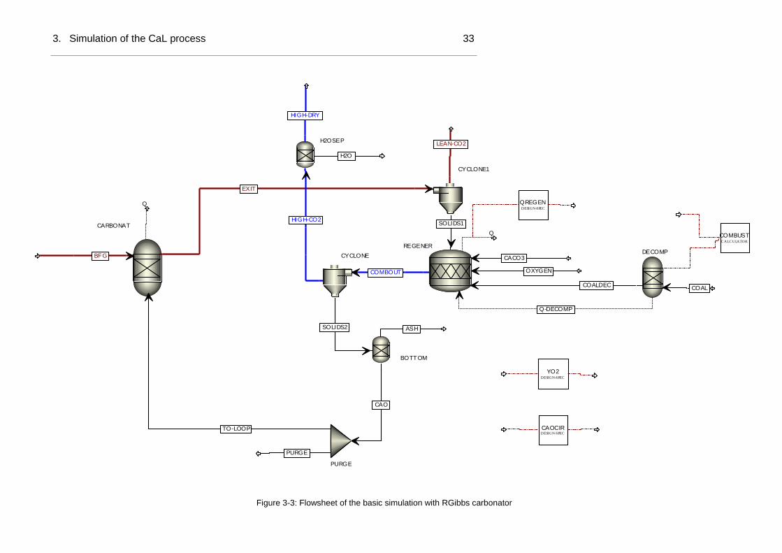
3. Simulation of the CaL process 33
Figure 3-3: Flowsheet of the basic simulation with RGibbs carbonator
CARBONAT
BFG
SOLIDS2
EXIT
LEAN-CO2
OXYGENCOMBOUT
SOLIDS1HIGH-CO2
PURGE
CACO3
REGENERDECOMP
COALCOALDEC
Q-DECOMP
TO-LOOP
C ALC ULATOR
COMBUST
CYCLONE
BOTTOM
ASH
CAO
CYCLONE1
QREG
Q
DESIGN-SPEC
QREGEN
DESIGN-SPEC
CAOCIR
H2OSEP
H2O
HIGH-DRY
QGASIFIC
Q
DESIGN-SPEC
YO2
PURGE

3. Simulation of the CaL process 34
3.2.4 Results of the basic model
The main outputs of the simulation are the volume flow of the flue gases and its composition.
Also the consumption of coal and oxygen in the regenerator are two key parameters that will
define the efficiency of the process.
Table 3-5: Flue gases compositions of the basic simulation with RGibbs carbonator
The total volume flow will be expressed in a standard volume (measured at 0°C and 1 atm).
Process gas: 28.613𝑘𝑚𝑜𝑙
ℎ×
22.4 𝑚3
𝑘𝑚𝑜𝑙= 640.93 Nm3/h
CO2-rich gas: 862.46 Nm3/h
The consumptions in the regenerator are presented in Table 3-6.
Table 3-6: Consumptions in the regenerator using RGibbs carbonator
Component Unit Value
Oxygen Nm³/h 420.45
Coal kg/h 386.55
Make-up kgCaCO3/h 66.06
Analyzing the composition of the CO2-lean flue gas and the flow of CO2 introduced in the
process, the carbon capture (ECO2) can be calculated:
𝐸𝐶𝑂2 =5.56 − 0.126
5.56= 97.7%
Another important output of the carbonator is the conversion of the CaO, (XCarb):
Process gas (CO2-lean) CO2-rich gas (dry)
[mol/h] [mol/h]
CO2 452 1.58% 36771 95.50%
CO 22295 77.92% - -
H2O - - 83 0.22%
H2 1217 4.25% - -
N2 3158 11.04% 144 0.37%
O2 - - 1401 3.64%
CH4 1491 5.21% - -
SO2
103 0.27%
Total 28613
38503
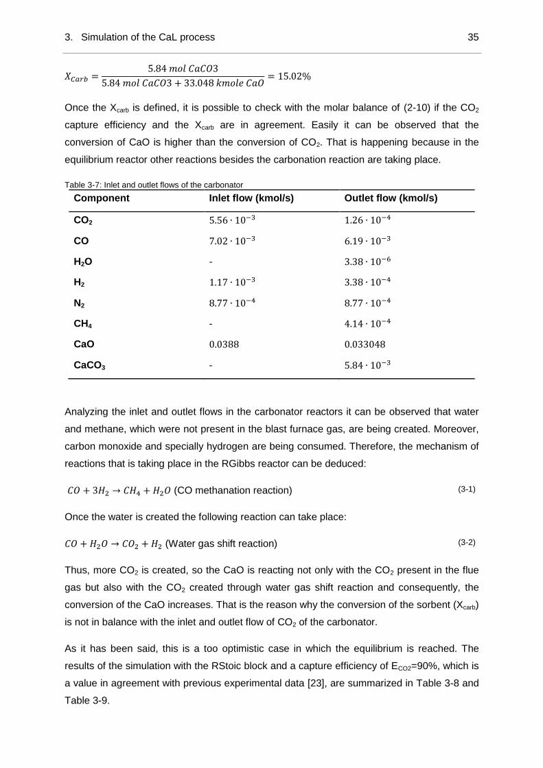
3. Simulation of the CaL process 35
𝑋𝐶𝑎𝑟𝑏 =5.84 𝑚𝑜𝑙 𝐶𝑎𝐶𝑂3
5.84 𝑚𝑜𝑙 𝐶𝑎𝐶𝑂3 + 33.048 𝑘𝑚𝑜𝑙𝑒 𝐶𝑎𝑂= 15.02%
Once the Xcarb is defined, it is possible to check with the molar balance of (2-10) if the CO2
capture efficiency and the Xcarb are in agreement. Easily it can be observed that the
conversion of CaO is higher than the conversion of CO2. That is happening because in the
equilibrium reactor other reactions besides the carbonation reaction are taking place.
Table 3-7: Inlet and outlet flows of the carbonator
Component Inlet flow (kmol/s) Outlet flow (kmol/s)
CO2 5.56 ∙ 10−3 1.26 ∙ 10−4
CO 7.02 ∙ 10−3 6.19 ∙ 10−3
H2O - 3.38 ∙ 10−6
H2 1.17 ∙ 10−3 3.38 ∙ 10−4
N2 8.77 ∙ 10−4 8.77 ∙ 10−4
CH4 - 4.14 ∙ 10−4
CaO 0.0388 0.033048
CaCO3 - 5.84 ∙ 10−3
Analyzing the inlet and outlet flows in the carbonator reactors it can be observed that water
and methane, which were not present in the blast furnace gas, are being created. Moreover,
carbon monoxide and specially hydrogen are being consumed. Therefore, the mechanism of
reactions that is taking place in the RGibbs reactor can be deduced:
𝐶𝑂 + 3𝐻2 → 𝐶𝐻4 + 𝐻2𝑂 (CO methanation reaction) (3-1)
Once the water is created the following reaction can take place:
𝐶𝑂 + 𝐻2𝑂 → 𝐶𝑂2 + 𝐻2 (Water gas shift reaction) (3-2)
Thus, more CO2 is created, so the CaO is reacting not only with the CO2 present in the flue
gas but also with the CO2 created through water gas shift reaction and consequently, the
conversion of the CaO increases. That is the reason why the conversion of the sorbent (Xcarb)
is not in balance with the inlet and outlet flow of CO2 of the carbonator.
As it has been said, this is a too optimistic case in which the equilibrium is reached. The
results of the simulation with the RStoic block and a capture efficiency of ECO2=90%, which is
a value in agreement with previous experimental data [23], are summarized in Table 3-8 and
Table 3-9.

3. Simulation of the CaL process 36
Table 3-8: Flue gases compositions of the basic simulation with RStoic carbonator
CO2-lean gas CO2-rich gas (dry)
[mol/h]
[mol/h]
CO2 2000 5.78% 33254 95.45%
CO 25264 72.95% - -
H2O - - 61 0.22%
H2 4211 12.16% - -
N2 3158 9.12% 147 0.39%
O2 - - 1224 3.66%
SO2 - - 44 0.28%
Total 34633
34731
Table 3-9: Consumptions in the regenerator using RStoic carbonator
Component Unit Value
Oxygen Nm³/h 400.59
Coal kg/h 263.52
Make-up kgCaCO3/h 66.06
𝑋𝐶𝑎𝑟𝑏 =5.00 × 10⁻³𝑚𝑜𝑙𝑒 𝐶𝑎𝐶𝑂3
5.00 × 10⁻³𝑚𝑜𝑙𝑒 𝐶𝑎𝐶𝑂3 + 3.3889 × 10⁻² 𝑚𝑜𝑙𝑒 𝐶𝑎𝑂= 12.86%
3.3 Energy integration
In a second step the heat integration of the CaL has been carried out from the basic
simulation with RStoic carbonator reactor that, as it has been seen, represents the most
realistic situation. Thus, the energy produced in the carbonator reactor and the energy of the
flue gases is utilized for heating up other streams of the process or steam production. As it
has been explained before, in the process proposed there are two main heat sources:
- Energy in the carbonator due to the exothermic reaction
- Energy of the CO2 flow leaving the regenerator at 900°C
On the other hand, the CO2-lean flue gas has to be split and heated up before its reinjection
into the blast furnace through the tuyeres. The version that showed best results in the first
ULCOS campaign has been taken as a reference to follow. Hence, the CO2-lean gas is
reinjected into the blast furnace in a 56% through the shaft tuyeres at approximately 900ºC
and 44% into the hearth of the blast furnace at higher temperature (1200°C).

3. Simulation of the CaL process 37
The energy extracted in the carbonator due to the exothermic reaction at 650°C will be used
to produce steam. The energy of the CO2 flue gas at 900°C will be used to heat in a first step
the process gas that leaves the carbonator at 650°C. However, after this first step the CO2-
rich flow is still having a lot of energy that can be extracted in the following steps, as
represented in flow diagram presented in Figure 3-4.
- Steam production (2)
- Blast furnace gas pre-heating
- Oxygen pre-heating (if the stream is hot enough)
For steam production the temperature of the flue gas has been reduced until 370°C. For
realistic heat exchangers dimensions the temperature gradient (ΔT) has been taken of
minimum 40°C. In addition, the outlet temperature of the flue gas has been considered
120°C. Lower temperatures would require as well too big heat exchangers with unrealistic
exchange surfaces.

3. Simulation of the CaL process 38
CARBONATOR
T=650°C
CO 72,95%
N2 9,12%
H2 12,16%
CO2 5,78%
Temp. 650°C
7 7 6 N m 3 / h
Top gas
CO 48,00%
CO2 38,00%
H2 8,00%
N2 6,00%
Temp. 110°C
1179 Nm3 /h REGENERATOR
T=900°C
CaCO3, CaO
CaO
O2
401 Nm3/h
20°C
CoalMake-up CaCO3
Ash, purge solids
CO2 95.76%
O2 3.52%
N2 0.42%
H2O 0.18%
SO2 0.13%
Temp. 900°C
7 7 8 N m 3 / h
Heater
850°C
1200°C
Blast
Furnace
Ore
Coke
Coal
Oyxgen
Hot metal
Slag
Heater
850°C
Heater
QNET
Q1
ASU
776°C370°C120°C
Q2
Q45
Q12
319°C
Figure 3-4: Energy integration of the CaL treating BFG

3. Simulation of the CaL process 39
3.3.1 Simulation in Aspen PlusTM
Continuing with the last flowsheet of the basic simulation with the RStoic reactor the energy
integration is simulated.
The stream of CO2 leaving the regenerator at 900°C “HIGH-DRY” is directed to a heater
block “HEATER1”. The stream “LEAN-CO2”, with low content of CO2 at 650°C, has to be
heated up before being reinjected into the blast furnace and is directed to another heater
block called “HEATER2”. The exit temperature of the cold stream, “HOT-LEAN”, is specified.
The stream is heated up until 850°C and a heat flow connecting “HEATER1” and
“HEATER2” is drawn (Q12). Therefore, the output temperature of the hot stream
“CO2COLD1” will be calculated.
This stream is still having a high temperature and is directed to the block “HEATER3” where
it is cooled down until 370°C. The released heat is represented with the heat flow “QS2” and
is used for steam production.
The stream leaving the heater “CO2COLD2” is at 370°C and will be used to pre-heat the
blast furnace gas “BFG”. This is done with two heater blocks (“HEATER4” and “HEATER5”)
connected with a heat stream (Q45) as it has been explained before.
3.3.2 Results of the simulation with heat integration
Table 3-10: Heat integration without CO2 recirculation
Process Streams T in (°C) T out (°C) Q (kW)
Steam Q1
(carbonator) - 650 650 1214.25
CO2-lean gas heating CO2-rich gas 900 775.6
65.64 CO2-lean gas 650 850
Steam Q2 CO2-rich gas 775.6 370 199.96
BFG pre-heating CO2-rich gas 370 120
107.53 BFG 110 318.7
The heat integration can have a certain influence in the coal consumption and as a result, in
the oxygen required in the regenerator. The coal consumption is expected to decrease
because of the pre-heating of the BFG. For this reason the composition of the CO2
concentrated flue gas also differs slightly from the previous simulation without heat
integration.
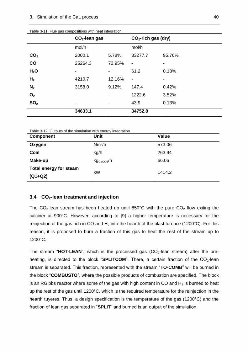
3. Simulation of the CaL process 40
Table 3-11: Flue gas compositions with heat integration
CO2-lean gas CO2-rich gas (dry)
mol/h
mol/h
CO2 2000.1 5.78% 33277.7 95.76%
CO 25264.3 72.95% - -
H2O - - 61.2 0.18%
H2 4210.7 12.16% - -
N2 3158.0 9.12% 147.4 0.42%
O2 - - 1222.6 3.52%
SO2 - - 43.9 0.13%
34633.1
34752.8
Table 3-12: Outputs of the simulation with energy integration
Component Unit Value
Oxygen Nm³/h 573.06
Coal kg/h 263.94
Make-up kgCaCO3/h 66.06
Total energy for steam
(Q1+Q2) kW 1414.2
3.4 CO2-lean treatment and injection
The CO2-lean stream has been heated up until 850°C with the pure CO2 flow exiting the
calciner at 900°C. However, according to [9] a higher temperature is necessary for the
reinjection of the gas rich in CO and H2 into the hearth of the blast furnace (1200°C). For this
reason, it is proposed to burn a fraction of this gas to heat the rest of the stream up to
1200°C.
The stream “HOT-LEAN”, which is the processed gas (CO2-lean stream) after the pre-
heating, is directed to the block “SPLITCOM”. There, a certain fraction of the CO2-lean
stream is separated. This fraction, represented with the stream “TO-COMB” will be burned in
the block “COMBUSTO”, where the possible products of combustion are specified. The block
is an RGibbs reactor where some of the gas with high content in CO and H2 is burned to heat
up the rest of the gas until 1200°C, which is the required temperature for the reinjection in the
hearth tuyeres. Thus, a design specification is the temperature of the gas (1200°C) and the
fraction of lean gas separated in “SPLIT” and burned is an output of the simulation.
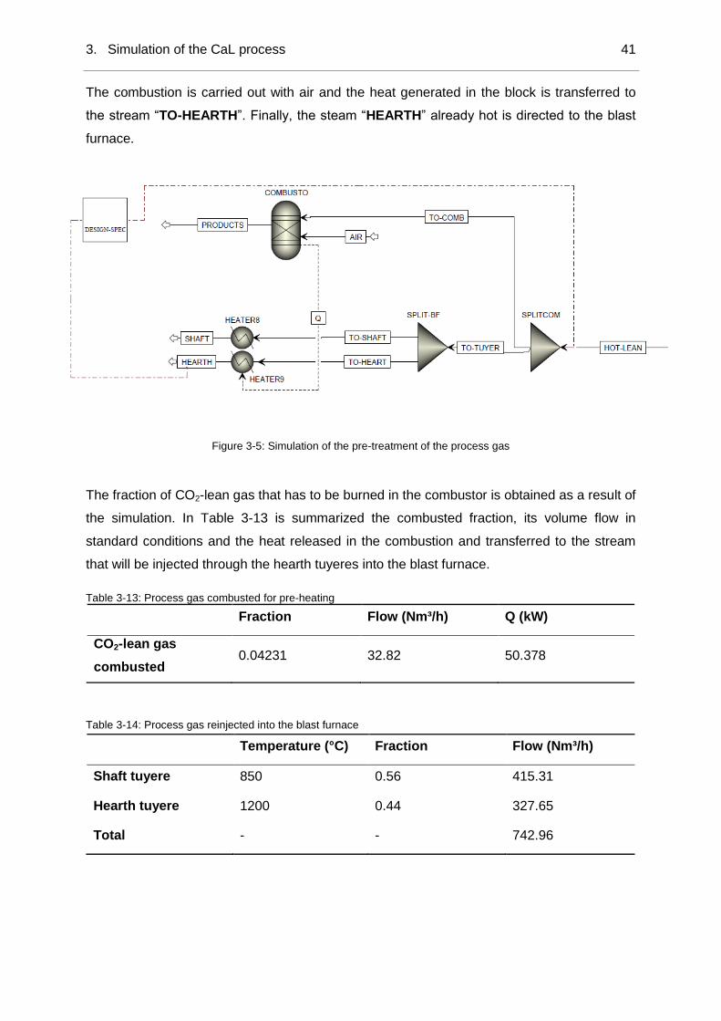
3. Simulation of the CaL process 41
The combustion is carried out with air and the heat generated in the block is transferred to
the stream “TO-HEARTH”. Finally, the steam “HEARTH” already hot is directed to the blast
furnace.
Figure 3-5: Simulation of the pre-treatment of the process gas
The fraction of CO2-lean gas that has to be burned in the combustor is obtained as a result of
the simulation. In Table 3-13 is summarized the combusted fraction, its volume flow in
standard conditions and the heat released in the combustion and transferred to the stream
that will be injected through the hearth tuyeres into the blast furnace.
Table 3-13: Process gas combusted for pre-heating
Fraction Flow (Nm³/h) Q (kW)
CO2-lean gas
combusted 0.04231 32.82 50.378
Table 3-14: Process gas reinjected into the blast furnace
Temperature (°C) Fraction Flow (Nm³/h)
Shaft tuyere 850 0.56 415.31
Hearth tuyere 1200 0.44 327.65
Total - - 742.96

3. Simulation of the CaL process 42
3.5 CO2 recirculation in the combustor
As it has been explained in chapter 2.5.1, the combustion only with oxygen is not possible
because too high flame temperatures are achieved. In a real facility the calcination should be
carried out with a certain amount of CO2 recirculated in the regenerator. Thus, for more
realistic results of coal and oxygen consumption this scenario has been simulated.
A 50% of recirculation of the CO2-rich flow has been proposed. The stream is recirculated
after extracting the heat for steam production. The Aspen PlusTM flowsheet is presented in
the Appendix in Figure 9-5.
The flowsheet is changed adding an SSplit block “CO2-SPLI” after the heat exchanger
“HEATER3”, in which the energy for steam production is extracted. In the splitter a
separation of 50% of the flow is set. The stream “CO2-LOOP” is directly recirculated into the
regenerator, while the other half of the flue gas is directed to the next heater where the blast
furnace gas will be pre-heated. No further changes are made in the simulation.
The main consequence of this change will be higher coal consumption. The reason for this is
that more energy will be required to heat up again the cold CO2-rich flow reinjected into the
calcinery. If the coal consumption is higher, the oxygen required for the oxy-fuel combustion
will be obviously also higher. At the same time, higher steam will be produced.
Table 3-15: Heat integration with CO2 recirculation in the calciner
Process Streams T in (°C) T out (°C) Q (kW)
Steam Q1
(carbonator) - 650 650 1223.53
CO2-lean gas
heating
CO2-rich gas 900 842.9 65.64
CO2-lean gas 650 850
Steam Q2 CO2-rich gas 842.9 370 508.55
BFG pre-heating CO2-rich gas 370 120
112.4 BFG 110 327.8
In Table 3-16 the main results of the simulation are presented. Those results will be used in
the following chapters for the calculations of the integration of the CaL in the steel mill and
the costs calculation.
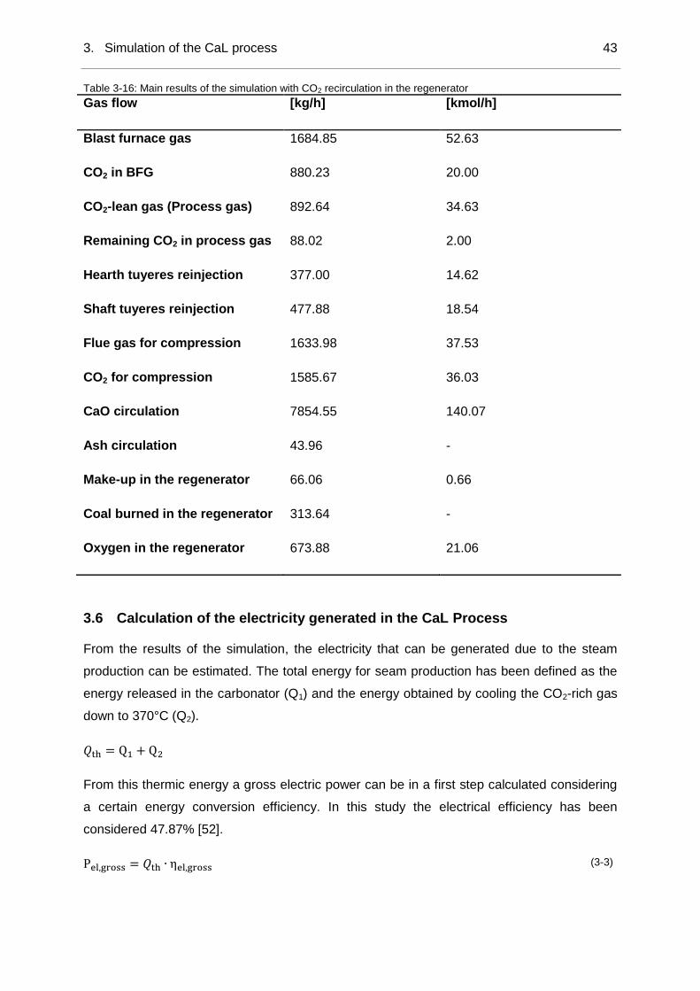
3. Simulation of the CaL process 43
Table 3-16: Main results of the simulation with CO2 recirculation in the regenerator
Gas flow [kg/h] [kmol/h]
Blast furnace gas 1684.85 52.63
CO2 in BFG 880.23 20.00
CO2-lean gas (Process gas) 892.64 34.63
Remaining CO2 in process gas 88.02 2.00
Hearth tuyeres reinjection 377.00 14.62
Shaft tuyeres reinjection 477.88 18.54
Flue gas for compression 1633.98 37.53
CO2 for compression 1585.67 36.03
CaO circulation 7854.55 140.07
Ash circulation 43.96 -
Make-up in the regenerator 66.06 0.66
Coal burned in the regenerator 313.64 -
Oxygen in the regenerator 673.88 21.06
3.6 Calculation of the electricity generated in the CaL Process
From the results of the simulation, the electricity that can be generated due to the steam
production can be estimated. The total energy for seam production has been defined as the
energy released in the carbonator (Q1) and the energy obtained by cooling the CO2-rich gas
down to 370°C (Q2).
𝑄th = Q1 + Q2
From this thermic energy a gross electric power can be in a first step calculated considering
a certain energy conversion efficiency. In this study the electrical efficiency has been
considered 47.87% [52].
Pel,gross = 𝑄th ∙ ηel,gross (3-3)

3. Simulation of the CaL process 44
This is the extra power generated due to the CaL CO2 capture process. However, the CO2
capture with Calcium Looping requires electricity for its own operation (𝑃𝐶𝑎𝐿,𝑜𝑤𝑛) and the CO2
compression necessary previous storage. As it has been explained in 2.5.1 a high amount of
electricity is necessary for the oxygen production in the Air Separation Unit (𝐸𝐴𝑆𝑈). Therefore,
the energy required for these processes will be subtracted from the gross power.
𝐸𝐴𝑆𝑈 = 0.33 𝑘𝑊ℎ
𝑁𝑚³𝑂2= 0.231
𝑘𝑊ℎ
𝑘𝑔 𝑂2
𝑃𝐴𝑆𝑈 = 0.231 ∙ ��𝑂2∙ 3600 [𝑘𝑊]
��𝑂2= oxygen flow consumed in the regenerator (kg/s).
Regarding the electricity required for the CO2 compression until 110 bara, the value of
177.8 kWh/t CO2 that has been used is in agreement with previous studies [48], [49].
𝑃𝐶𝑂2 𝑐𝑜𝑚𝑝𝑟𝑒𝑠𝑠𝑖𝑜𝑛 = 0.1778 ∙ ��𝐶𝑂2∙ 3600 [𝑘𝑊]
��𝐶𝑂2= CO2 flow for compression and storage (kg/s).
This way, the net power generated in the CaL process that can be used in other sections of
the steel mill can be defined as:
𝑃𝑒𝑙,𝑛𝑒𝑡 = Pel,gross − 𝑃𝐴𝑆𝑈 − 𝑃𝐶𝑂2 𝑐𝑜𝑚𝑝𝑟𝑒𝑠𝑠𝑖𝑜𝑛 − 𝑃𝐶𝑎𝐿,𝑜𝑤𝑛[𝑘𝑊] (3-4)
ηel,net = 𝑃𝑒𝑙,𝑛𝑒𝑡
𝑄th [%]
(3-5)
For the calculation of the extra energy that can be produced with the Calcium Looping cycle
two scenarios have been proposed. The first one makes reference to the results obtained
without the CO2 recirculation in the regenerator (see chapter 3.3). The second scenario
makes reference to the simulation considering a more realistic case where a 50% of the cold
CO2 is recirculated into the regenerator (see chapter 3.5.) for the oxy-fuel combustion. As it
has been seen before, this second scenario implies higher coal consumption, but at the
same time a higher amount of energy is recovered for steam production.

3. Simulation of the CaL process 45
Table 3-17: Electricity production in the two different scenarios
Scenario 1 (without CO2
recirculation)
Scenario 2 (with 50% of
CO2 recirculation)
𝐐𝒕𝒉 [MW] 1.414 1.732
𝛈𝐞𝐥,𝐠𝐫𝐨𝐬𝐬 47.87% 47.87%
𝐏𝐞𝐥,𝐠𝐫𝐨𝐬𝐬 [kW] 676.98 829.15
𝑷𝑨𝑺𝑼 [kW] 132.38 155.67
𝑷𝑪𝑶𝟐 𝒄𝒐𝒎𝒑𝒓𝒆𝒔𝒔𝒊𝒐𝒏 [kW] 178.08 192.48
𝑷𝒆𝒍,𝒏𝒆𝒕 [kW] 366.53 481.00
𝛈𝐞𝐥,𝐧𝐞𝐭 25.92% 27.77%
The results showed in Table 3-17 make reference to the outputs of the simulation. As it has
been said, the simulation has been carried out for the treatment of the gas generated in the
production of one ton of hot metal during one hour. Thus, the energy that can be produced
by the treatment of the BFG in the CaL is:
- 366.5 kWh/thm for the first scenario without CO2 recirculation
- 481 kWh/thm for the second scenario with CO2 recirculation.

4. Energetic comparison of CO2 capture technologies 46
4 Energetic comparison of CO2 capture technologies
4.1 General statements
Calcium Looping has been evaluated and a simulation of its operation under the conditions
of a Top Gas Recycling Blast Furnace has been carried out. In this chapter a comparison of
this technology with the current state of the art technologies for CO2 capture in steel industry
will be accomplished.
As it has been explained in the theoretical background, the most promising solution
regarding emissions reduction in the steel industry was proposed by ULCOS program. On
the other hand, the IEA Green House Gas Programme (IEAGHG) carried out a study in July
2013 evaluating technically and economically CCS for an integrated steel mill [12]. A review
of the report made by ULCOS was included in the study.
ULCOS proposed the already explained VPSA system as CO2 capture method, whereas in
the study of the IEAGHG the evaluated capture method was a chemical absorption
technology of amines using as a solvent MDEA activated by Piperazine.
The first method, VPSA, has been tested in the first campaigns of ULCOS Experimental
Blast Furnace of LKAB [7], [53]. The MDEA/Pz method proposed by IEAGHG has not been
tested experimentally in a Top Gas Recycling Blast Furnace but this capture method has
been widely used in separation of CO2 from gas natural extraction and its performance and
costs are well documented. Table 4-1 summarizes a comparison of the different actual CO2
capture technologies proposed for an Integrated Steel Mill (BF-BOF Route), presented by
[11].
In this chapter these two CO2 capture methods and the CaL will be compared calculating the
required energy for the CO2 capture for each of them.
Table 4-1: Comparison of CO2 capture technologies for an Integrated Steel Mill [11], [12][12][12]
PSA VPSA
VPSA&Cryo.
Flash and
Compression
Amines and
Compression
VPSA&Cryo.
Distil. and
Compression
Recycled Top Gas (Process Gas)
CO yield % 88.0 90.4 97.3 99.9 100.0
Process Gas
Composition
CO2 %w 2.7 3 3 2.9 2.7
CO %w 71.4 69.2 68.9 67.8 69.5
H2 %w 12.4 13 12.6 12.1 12.4
N2 %w 13.5 15.7 15.6 15.1 15.4

4. Energetic comparison of CO2 capture technologies 47
H2O %w 0 0 0 2.1 0
Captured CO2 Rich Gas
CO2 %w 79.7 87.2 96.3 100 100
CO %w 12.1 10.7 3.3 0 0
H2 %w 2.5 0.6 0.1 0 0
N2 %w 5.6 1.6 0.3 0 0
Suitable for CO2 Transport &
Storage? No No Yes (?) Yes Yes
Electricity
consumption
Capture Process kWh/tCO2 100 105 160 55 195
CO2 Compression
(110 bara) kWh/tCO2 - - 132 115 115
LP Steam
Consumption GJ/tCO2 0 0 0 3.2 0
Total Energy
Consumption GJ/tCO2 0.36 0.38 1.05 3.81 1.12
One of the requirements for the use of the technologies is that the concentration of the CO2
for transport and storage has to be higher than 95%. This requirement excludes the
utilization of PSA or VPSA individually as a CO2 capture method. VPSA technology has to be
complemented by a cryogenics unit designed to purify the CO2 stream, i.e. fractional
liquefaction of the gas.
4.1.1 Energetic cost of CaL CO2 capture
The objective of this chapter is to calculate the energy utilized for the CO2 capture in the CaL
process to make a comparison with the previously presented alternative methods and
evaluate the convenience of one or another method.
As it has been seen before, one of the particularities of the CaL process is that unlike the
other CCS technologies here presented, it enables the recovery of energy for steam
production. When this process is used as a post-combustion CO2 capture unit in a power
plant a significant increase of the electricity produced is achieved. Hence, for the calculation
of the energy required for the capture, only the energy utilized for CO2 capture and not all the
energy introduced in the system will be considered.
The main input of energy in the process is the coal introduced in the regenerator reactor. The
energy introduced as coal can be easily calculated with its lower heating value. Of this

4. Energetic comparison of CO2 capture technologies 48
energy, one part will be recovered in the form of steam, so this energy will be subtracted
from the total energy input. The other energy recovery in the process is the heating of the
CO2-lean gas up to 850°C previous its reinjection in the blast furnace. This energy comes
from the CO2 flue gas and has to be subtracted from the total energy input because it is not
an inherent process of the Calcium Looping capture. If this pre-heating were not done, like in
the case of the other capture methods, more steam would be produced but an extra heater
would be required.
Once this is done, the resulting energy input will be considered as energy for CO2 capture.
Part of this energy is used for heating up streams and solids, another part is required for the
endothermic reaction and some energy is just lost in the flue gases and in the purge.
For the calculation of the energetic cost of the CO2 capture with Calcium Looping the results
of the simulation with Aspen PlusTM will be utilized. It has to be reminded, that these results
make reference to the treatment of the flue gas generated in the production of one ton of hot
metal in one hour.
Table 4-2: Energetic cost of CaL CO2 capture
Units
Without
recirculation With recirculation
Coal consumption [kg/h] 263.94 313.64
Heat of combustion, LHV [kJ/kgcoal] 27214.2 27214.2
Energy introduced as coal [MW] 1.995 2.371
Steam produced [MW] 1.414 1.732
Energy for CO2-lean gas pre-
heating [kW] 65.64 65.64
Energy for CO2 capture [kW] 515.42 573.23
CO2 captured [kg/h] 792.2 792.2
Energy required per CO2
captured [kWh/tCO2 captured] 650.6 723.6
Efficiency steam production [Qth steam/Qth coal] 0.7088 0.7305
The other point of the Calcium Looping process with large energy consumption is the air
separation unit, which requires electricity for the production of oxygen used in the oxy-fuel
combustion. The air separation unit, which is an essential unit in an oxygen blast furnace, will
have a higher electricity consumption in order to provide this necessary extra oxygen for the
CaL. The operation and energy requirements of the unit were described in chapter 2.5.1.
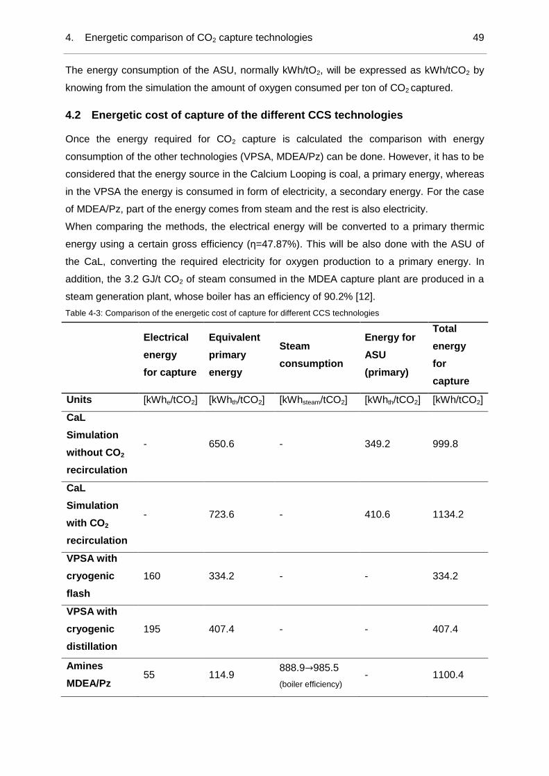
4. Energetic comparison of CO2 capture technologies 49
The energy consumption of the ASU, normally kWh/tO2, will be expressed as kWh/tCO2 by
knowing from the simulation the amount of oxygen consumed per ton of CO2 captured.
4.2 Energetic cost of capture of the different CCS technologies
Once the energy required for CO2 capture is calculated the comparison with energy
consumption of the other technologies (VPSA, MDEA/Pz) can be done. However, it has to be
considered that the energy source in the Calcium Looping is coal, a primary energy, whereas
in the VPSA the energy is consumed in form of electricity, a secondary energy. For the case
of MDEA/Pz, part of the energy comes from steam and the rest is also electricity.
When comparing the methods, the electrical energy will be converted to a primary thermic
energy using a certain gross efficiency (η=47.87%). This will be also done with the ASU of
the CaL, converting the required electricity for oxygen production to a primary energy. In
addition, the 3.2 GJ/t CO2 of steam consumed in the MDEA capture plant are produced in a
steam generation plant, whose boiler has an efficiency of 90.2% [12].
Table 4-3: Comparison of the energetic cost of capture for different CCS technologies
Electrical
energy
for capture
Equivalent
primary
energy
Steam
consumption
Energy for
ASU
(primary)
Total
energy
for
capture
Units [kWhe/tCO2] [kWhth/tCO2] [kWhsteam/tCO2] [kWhth/tCO2] [kWh/tCO2]
CaL
Simulation
without CO2
recirculation
- 650.6 - 349.2 999.8
CaL
Simulation
with CO2
recirculation
- 723.6 - 410.6 1134.2
VPSA with
cryogenic
flash
160 334.2 - - 334.2
VPSA with
cryogenic
distillation
195 407.4 - - 407.4
Amines
MDEA/Pz 55 114.9
888.9→985.5
(boiler efficiency) - 1100.4

4. Energetic comparison of CO2 capture technologies 50
It can be seen that the CaL process offers similar energetic penalties than the amines
absorption. The amines method requires steam and electricity that have to be produced
elsewhere in the steel mill whereas the only consumption of the CaL is the coal that is
burned in the process.
Compared to the VPSA technology the energetic cost of capture with the CaL process,
including the required energy for the ASU, is higher. However, the VPSA technology is based
on membranes and consumes electricity that has to be imported from the grid or has to be
produced in a power plant adding economic penalties or complexity to the process. In
addition, the sorbents used in the VPSA technology are not very resistant towards impurities
in the off-gas. In contrast, the sorbent used in the CaL process is very robust and cheap.
Although the VPSA method offers lower energy penalties of capture than CaL process, in
terms of complexity, economic viability or CO2 emission the CaL process could be
considered as an alternative solution. These facts will be analyzed in the following points of
the project.

5. Implementation of the CaL in the steel mill 51
5 Implementation of the CaL in the steel mill
5.1 Scaling of the plant
For the study of the implementation of Calcium Looping process in a steel mill, in a first step
a scaling of the CaL simulated plant to the real size required for a steel mill has to be done.
The second simulated scenario, with CO2 recirculation in the calciner, will be used for the
implementation of the CaL in the steel mill and the economic viability study.
For the scaling to a real steel mill, the capacity of the steel mill is necessary. The steel mill
has been considered a typical Western European plant, with an annual production of 4
million tons of hot rolled coil (HRC). On the other hand, this reference mill works constantly,
i.e. annual operating hours are 8760 h. The economic life of the steel mill will be considered
equal to 25 years. The characteristics of the reference steel mill are the same as the steel
mill presented in the IEA study in order to make possible a comparison between both
technologies and their implementation in the steel industry [12].
As it has been discussed previously, the simulation has been carried out for the treatment of
the gases generated per ton of hot metal produced, and in the implementation to Aspen
PlusTM, this was considered as a flow per hour. Once this is assumed, the inlet and outlet
flows obtained in the simulation with CO2 recirculation will be resized to the reference steel
mill.
Table 5-1: Characteristics of the reference steel mill
Unit Value
Capacity [tons HRC/year] 4,000,000
Relation iron ore/hot rolled coil [thm/t HRC] 0.9735
Operating hours [hours/year] 8760
Production of the blast furnace [thm/hour] 444.52
The most important flows are summarized in Table 5-2:
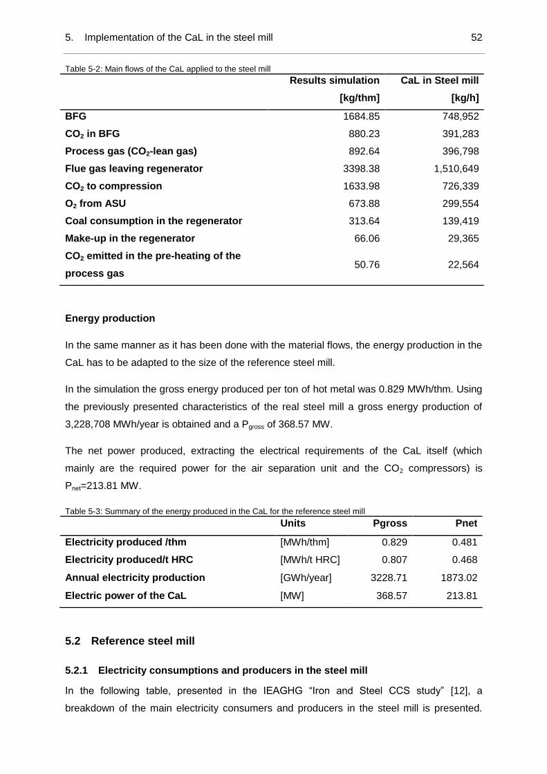
5. Implementation of the CaL in the steel mill 52
Table 5-2: Main flows of the CaL applied to the steel mill
Results simulation
[kg/thm]
CaL in Steel mill
[kg/h]
BFG 1684.85 748,952
CO2 in BFG 880.23 391,283
Process gas (CO2-lean gas) 892.64 396,798
Flue gas leaving regenerator 3398.38 1,510,649
CO2 to compression 1633.98 726,339
O2 from ASU 673.88 299,554
Coal consumption in the regenerator 313.64 139,419
Make-up in the regenerator 66.06 29,365
CO2 emitted in the pre-heating of the
process gas 50.76 22,564
Energy production
In the same manner as it has been done with the material flows, the energy production in the
CaL has to be adapted to the size of the reference steel mill.
In the simulation the gross energy produced per ton of hot metal was 0.829 MWh/thm. Using
the previously presented characteristics of the real steel mill a gross energy production of
3,228,708 MWh/year is obtained and a Pgross of 368.57 MW.
The net power produced, extracting the electrical requirements of the CaL itself (which
mainly are the required power for the air separation unit and the CO2 compressors) is
Pnet=213.81 MW.
Table 5-3: Summary of the energy produced in the CaL for the reference steel mill
Units Pgross Pnet
Electricity produced /thm [MWh/thm] 0.829 0.481
Electricity produced/t HRC [MWh/t HRC] 0.807 0.468
Annual electricity production [GWh/year] 3228.71 1873.02
Electric power of the CaL [MW] 368.57 213.81
5.2 Reference steel mill
5.2.1 Electricity consumptions and producers in the steel mill
In the following table, presented in the IEAGHG “Iron and Steel CCS study” [12], a
breakdown of the main electricity consumers and producers in the steel mill is presented.

5. Implementation of the CaL in the steel mill 53
The proposed steel mill, with a Top Gas Recycling Blast Furnace (TGR-BF) and using
MDEA/Pz absorption as a CO2 capture method, is compared with a reference regular steel
mill without CO2 capture. The base case fits the electrical requirements producing its own
electricity in a power plant. In it, flue gases generated in the process (Blast Furnace Gas and
Basic Oxygen Furnace Gas) together with natural gas are burnt. This power plant is
considered to be part of the steel mill and enough to supply the requirements of the whole
steel mill. Therefore, there is no import or export of electricity out of the boundary limit. This
is considered for an easier study of the entire process, taking into account the direct and
indirect CO2 emissions in the steel production.
Table 5-4: Electricity demand and supply of the steel mill without and with CO2 capture[12] [Table C-8]
Unit Reference Steel Mill without
CO2 capture
Steel Mill with MDEA
CO2 capture
Electricity production 400.1 kWh/t HRC 573.4 kWh/t HRC
Power Plant type Gas Fired Boiler Power Plant Natural Gas Combined
Cycle
Fuel type BFG (66%), BOFG (15%), NG
(19%) NG (100%)
Average daily net power output 183 MWe 262 MWe
Net efficiency 32.2 % 56.6 %
Electricity demand [kWh/t HRC] [kWh/t HRC]
Coke production 14.3 10.9
Sinter plant 35.6 34.8
Iron making 98.1 29.8
Steelmaking 48.8 48.8
Continuous casting 10.9 10.9
Reheating and rolling 105.3 105.3
Lime Production 2.6 2.6
ASU HP Oxygen 66.8 38
ASU LP Oxygen - 120.3
Ancillary 4.8 4.8
Steam Generation Plant - 11.0
CO2 Capture & Compression - 143.2
Offsite Users and Losses 13.1 13.1
For the alternative case with CO2 capture, an expansion of the power plant is required to
provide the additional electricity demand. This rise in the electricity demand is caused
basically by the following reasons:
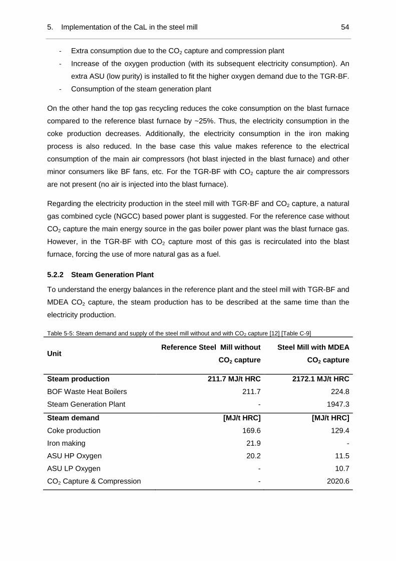
5. Implementation of the CaL in the steel mill 54
- Extra consumption due to the CO2 capture and compression plant
- Increase of the oxygen production (with its subsequent electricity consumption). An
extra ASU (low purity) is installed to fit the higher oxygen demand due to the TGR-BF.
- Consumption of the steam generation plant
On the other hand the top gas recycling reduces the coke consumption on the blast furnace
compared to the reference blast furnace by ~25%. Thus, the electricity consumption in the
coke production decreases. Additionally, the electricity consumption in the iron making
process is also reduced. In the base case this value makes reference to the electrical
consumption of the main air compressors (hot blast injected in the blast furnace) and other
minor consumers like BF fans, etc. For the TGR-BF with CO2 capture the air compressors
are not present (no air is injected into the blast furnace).
Regarding the electricity production in the steel mill with TGR-BF and CO2 capture, a natural
gas combined cycle (NGCC) based power plant is suggested. For the reference case without
CO2 capture the main energy source in the gas boiler power plant was the blast furnace gas.
However, in the TGR-BF with CO2 capture most of this gas is recirculated into the blast
furnace, forcing the use of more natural gas as a fuel.
5.2.2 Steam Generation Plant
To understand the energy balances in the reference plant and the steel mill with TGR-BF and
MDEA CO2 capture, the steam production has to be described at the same time than the
electricity production.
Table 5-5: Steam demand and supply of the steel mill without and with CO2 capture [12] [Table C-9]
Unit Reference Steel Mill without
CO2 capture
Steel Mill with MDEA
CO2 capture
Steam production 211.7 MJ/t HRC 2172.1 MJ/t HRC
BOF Waste Heat Boilers 211.7 224.8
Steam Generation Plant - 1947.3
Steam demand [MJ/t HRC] [MJ/t HRC]
Coke production 169.6 129.4
Iron making 21.9 -
ASU HP Oxygen 20.2 11.5
ASU LP Oxygen - 10.7
CO2 Capture & Compression - 2020.6
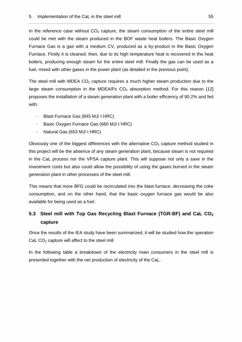
5. Implementation of the CaL in the steel mill 55
In the reference case without CO2 capture, the steam consumption of the entire steel mill
could be met with the steam produced in the BOF waste heat boilers. The Basic Oxygen
Furnace Gas is a gas with a medium CV, produced as a by-product in the Basic Oxygen
Furnace. Firstly it is cleaned; then, due to its high temperature heat is recovered in the heat
boilers, producing enough steam for the entire steel mill. Finally the gas can be used as a
fuel, mixed with other gases in the power plant (as detailed in the previous point).
The steel mill with MDEA CO2 capture requires a much higher steam production due to the
large steam consumption in the MDEA/Pz CO2 absorption method. For this reason [12]
proposes the installation of a steam generation plant with a boiler efficiency of 90.2% and fed
with:
- Blast Furnace Gas (845 MJ/ t HRC)
- Basic Oxygen Furnace Gas (660 MJ/ t HRC)
- Natural Gas (653 MJ/ t HRC)
Obviously one of the biggest differences with the alternative CO2 capture method studied in
this project will be the absence of any steam generation plant, because steam is not required
in the CaL process nor the VPSA capture plant. This will suppose not only a save in the
investment costs but also could allow the possibility of using the gases burned in the steam
generation plant in other processes of the steel mill.
This means that more BFG could be recirculated into the blast furnace, decreasing the coke
consumption, and on the other hand, that the basic oxygen furnace gas would be also
available for being used as a fuel.
5.3 Steel mill with Top Gas Recycling Blast Furnace (TGR-BF) and CaL CO2
capture
Once the results of the IEA study have been summarized, it will be studied how the operation
CaL CO2 capture will affect to the steel mill.
In the following table a breakdown of the electricity main consumers in the steel mill is
presented together with the net production of electricity of the CaL.

5. Implementation of the CaL in the steel mill 56
Table 5-6: Electricity demand and supply of the steel mill with CaL CO2 capture
Unit Steel Mill with CaL CO2 capture
Electricity production [kWh/t HRC]
Electricity produced in CaL (net) 468.3
Electricity demand [kWh/t HRC]
Coke production 10.9
Sinter plant 34.8
Iron making 29.8
Steelmaking 48.8
Continuous casting 10.9
Reheating and rolling 105.3
Lime Production 2.6
ASU HP Oxygen1 38
ASU LP Oxygen2 120.3
Ancillary 4.8
Offsite Users and Losses 13.1
Total demand 419.3
An important fact to take into account is the unique characteristic of the CaL, which enables
the production of electricity. The net electricity produced by the Calcium Looping plant is
enough to meet the electrical requirements of the complete steel mill. This net electricity
production was presented in Table 5-3 and includes the own consumption of the CaL
process (ASU and CO2 compression).
The CaL capture plant, unlike the MDEA technology, does not require steam for the CO2
separation. The demand of steam of the steel mill using this technology will be drastically
reduced compared to the steel mill with MDEA capture. Therefore, the low demand of steam
can be covered, as it was done in the reference plant without CO2 capture, with the waste
heat boilers of the Basic Oxygen Furnace. Thus, the steam generation plant is not needed.
The avoidance of the steam generation plant will decrease also the electricity demand of the
steel mill (as it is detailed in Table 5-4, the steam generation plant requires some electricity).
1
The consumptions of the HP and LP ASU have been taken equal to the values presented in the IEA study. However, experts have noted that this is a too pessimistic value. For HP oxygen, 0.48 kWh/Nm
3
would be more realistic, resulting in a consumption of: 33.2 kWh/t HRC. 2 For the LP oxygen, a value of 0.33 kWh/Nm
3 would be more realistic, resulting in the consumption of:
84.5 kWh/t HRC.

5. Implementation of the CaL in the steel mill 57
In Table 5-7 the steam demand and supply of the steel mill with CaL for CO2 capture is
presented.
Table 5-7: Steam demand and supply of the steel mill with CaL CO2 capture
UNIT Steel Mill with CaL CO2 capture
Steam production [MJ/t HRC]
BOF waste heat boilers 224.8
Steam demand [MJ/t HRC]
Coke Production 129.4
ASU HP Oxygen 11.5
ASU LP Oxygen 28.455
Total steam demand 169.36
5.4 Steel mill with TGR-BF and VPSA CO2 capture
In case of using VPSA as CO2 capture technology, the steel mill would also present some
differences compared to the steel mill with MDEA. The electricity consumption of the VPSA
capture plants is 3~4 times higher than the MDEA/Pz installation (which consumes mainly
steam). For this reason, an expansion of the power plant is necessary. As it has been
proposed in the steel mill with TGR-BF and MDEA by [12], a natural gas combined cycle will
be used to provide the electricity to the steel mill.
The electricity consumption of the VPSA capture & compression plant has been presented in
Table 4-1. The case of VPSA with cryogenic distillation is chosen (310 kWh/t CO2). This
value will replace the electrical consumption of the MDEA CO2 capture plant presented in
Table 5-4.
In the same manner as in the CaL previously discussed, the steam generation plant is not
required for the steel mill with VPSA. The avoidance of the steam generation plant means
the saving of its electricity consumption. The electricity demand of the steel mill TGR-BF and
VPSA is estimated to be 684.9 kWh/t HRC. Once the energy consumption of the steel mill
has been calculated, the net power of the natural gas combined cycle for this steel mill can
be determined. This net power is equal to 312.7 MWe,net.
5.5 CO2 emissions in the Steel mill
Although the TGR-BF implies much lower CO2 emissions for the iron production, the
emissions in other parts of the steel mill are still relevant. As it has been explained before,
the CCS process is installed in the BF because it is the main source of CO2 emissions.
However, as it was presented in Figure 2-1, the steel mill comprises lots of process involving

5. Implementation of the CaL in the steel mill 58
combustion where CO2 is emitted. For this reason, even if high CO2 capture rates are
achieved in the CCS process, the CO2–emission reduction of the whole steel plant will not be
that high. In addition, it should be again remarked that the emissions that have been
estimated in this chapter do not consider the CO2-loss typically produced during the
compression of the captured CO2 (around 5% of the compressed gas).
The steel mill defined by the IEA, using MDEA for capture, produces the electricity in a
natural gas combined cycle (57% efficiency), whose emissions are 211.1 kg CO2/t HRC. This
is equal to an annual CO2 emission of 844,400 t CO2. Besides the CO2 emission in the power
plant, the IEA steel mill produces the required steam for CO2 capture in the steam generation
plant, where natural gas and other process gases (BFG and BOFG) are burned. The
emissions of this plant are estimated at 280.12 kg CO2/t HRC. That amounts to 1,120,480
tons of CO2 per year.
If VPSA is used for carbon capture, as proposed by ULCOS [9], the electricity for the steel
mill operation and the capture plant has to be produced in the steel mill or imported from the
grid to balance steel plant needs. In this study, for the comparison of the three methods of
CO2 capture using the same assumptions, the electricity is produced in the steel mill using a
natural gas combined cycle, which has associated CO2 emissions.
The steel mill using CaL as CCS technology offers an important advantage in front of the
other methods. The electricity produced in the CaL, which as it has been seen is enough to
meet the steel mill demand, is an energy produced with “zero” emissions. Rigorously, the
electricity production of the CaL generates CO2 when combusting the coal in the regenerator.
However, the generated CO2 in the oxy-fuel combustion is obtained as a flow of pure CO2
that will be stored, being the CO2 emission to the atmosphere nearly zero. This makes CaL a
really attractive option for CO2 capture in the steel industry, being able to achieve
substantially lower CO2-emissions than the other proposed technologies, and this is, in the
end, the purpose of the project. The total CO2 emissions of a steel mill using the different
carbon capture technologies will be calculated using as a base the reference steel mill
proposed by the IEA [12].
For the reference steel mill without CO2 capture, the main sources of CO2 are from the flue
gases of the hot stoves, the power plant, the sinter plant, the coke ovens and the lime kilns.
These five sources generate 90% of the emissions of the steel mill.

5. Implementation of the CaL in the steel mill 59
Table 5-8: Breakdown of CO2 emissions- Reference steel mill [12]
CO2 emissions breakdown-
Major Processes
Emissions
[kg/t HRC]
Annual emission
[t CO2/year]
Coke oven 194.67 778,680
Flue gas-Sinter plant 289.46 1,157,840
Flue gas-Hot Stoves 415.19 1,660,760
Flare-Blast Furnace 19.73 78,920
Flue gas-Lime plant 71.62 286,480
Flue gas Power Plant 982.13 3,928,520
Other 121.33 485,320
Total 2094.14 8,376,560
The addition of a CO2 capture plant based on MDEA technology combined with the top gas
recycling enables the reduction of the CO2 emission by 46.6%, compared to the reference
steel mill. This reduction is caused by a reduction of the emissions in the blast furnace, as
well as in the coke oven because of the reduction in the coke consumption in the furnace.
Table 5-9: Breakdown of CO2 emissions- Steel mill using MDEA CO2 capture [12]
Emissions
[kg/t HRC]
Annual emission
[t CO2/year]
Coke oven 125.09 500,360
Flue gas-Sinter plant 265.65 1,062,600
Flue gas-Hot Stoves - -
Flue gas-TGR Process Gas
Fired Heaters 43.05 172,200
Flue gas-Lime plant 71.43 285,720
Flue gas Power Plant 211.1 3,928,520
Flue gas- Steam generation Plant 280.12 1,120,480
Other 122.31 489,240
Total 1118.75 4,475,000
The power plant required for the VPSA steel mill, with a higher generation than the one in the
MDEA steel mill, will have more CO2 emissions. The emissions of the power plant have been
recalculated for the new power plant. On the other hand, the emissions of the steam
generation plan are avoided in the VPSA steel mill.
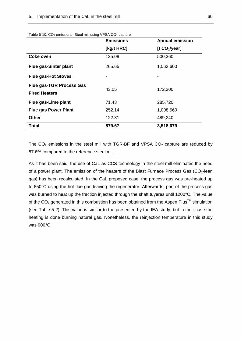
5. Implementation of the CaL in the steel mill 60
Table 5-10: CO2 emissions- Steel mill using VPSA CO2 capture
The CO2 emissions in the steel mill with TGR-BF and VPSA CO2 capture are reduced by
57.6% compared to the reference steel mill.
As it has been said, the use of CaL as CCS technology in the steel mill eliminates the need
of a power plant. The emission of the heaters of the Blast Furnace Process Gas (CO2-lean
gas) has been recalculated. In the CaL proposed case, the process gas was pre-heated up
to 850°C using the hot flue gas leaving the regenerator. Afterwards, part of the process gas
was burned to heat up the fraction injected through the shaft tuyeres until 1200°C. The value
of the CO2 generated in this combustion has been obtained from the Aspen PlusTM simulation
(see Table 5-2). This value is similar to the presented by the IEA study, but in their case the
heating is done burning natural gas. Nonetheless, the reinjection temperature in this study
was 900°C.
Emissions
[kg/t HRC]
Annual emission
[t CO2/year]
Coke oven 125.09 500,360
Flue gas-Sinter plant 265.65 1,062,600
Flue gas-Hot Stoves - -
Flue gas-TGR Process Gas
Fired Heaters 43.05 172,200
Flue gas-Lime plant 71.43 285,720
Flue gas Power Plant 252.14 1,008,560
Other 122.31 489,240
Total 879.67 3,518,679

5. Implementation of the CaL in the steel mill 61
Table 5-11: Breakdown of CO2 emissions- Steel mill using CaL CO2 capture
The CO2-emissions of the steel mill using CaL as CO2 capture technology are reduced by
69.7% compared to the reference mill, becoming this technology the best option if only the
avoidance of CO2 is considered. An additional advantage that the CaL technology could offer
is the fact that the purge of CaO generated in the CaL plant could be reused in the sinter
plant. This would decrease its CO2 emission, in part consequence of the calcination of
limestone that is done in this plant, and the global CO2 emission of the steel mill could be
even lower.
Table 5-12: Summary of the total emissions of the steel mill using different CO2 capture technologies
Case Production of electricity Total emissions
[kg/t HRC]
Reduction
[%]
Reference steel mill Gas Boiler Power Plant (natural
gas and flue gases) - 183 MWe 2094.14 -
Steel mill with
MDEA/Pz CO2
capture [IEA]
Natural Gas Combined Cycle
Power Plant – 262 MWe 1118.75 46.6
Steel mill with
VPSA CO2 capture
Natural Gas Combined Cycle
Power Plant – 312.7 MWe 879.67 58.0
Steel mill with CaL
CO2 capture Recovered from CaL 633.89 69.7
Emissions
[kg/t HRC]
Annual emission
[t CO2/year]
Coke oven 125.09 500,360
Flue gas-Sinter plant 265.65 1,062,600
Flue gas-Hot Stoves - -
Flue gas-TGR Process Gas
Fired Heaters 49.41 197,640
Flue gas-Lime plant 71.43 285,720
Other 122.31 489,240
Total 633.89 2,535,579

6. Economic comparison with other CO2 capture technologies 62
6 Cost of the Calcium Looping plant
Once the size of the CaL plant required for the reference steel mill is known, its capital and
operating costs can be calculated. Thus, the influence of the different costs to the total cost
can be determined through the cost analysis during the period under consideration. In the
following chapter the investment- and operating costs of the Calcium Looping plant will be
calculated.
6.1 Capital costs of the CaL facility
Because of the high complexity of the Calcium-Looping plant, the investment costs cannot be
directly deduced through comparison with comparable plants. Accordingly, for the
determination of the investment costs the cost of the main units of the CaL facility will be
estimated. The main units of the CaL are:
- Carbonator
- Regenerator
- Air separation unit (ASU)
- CO2 compression unit
- Other components of the facility (Steam turbine, fuel- and ash system, pipelines,
electric system, cooling system, etc.)
Investment cost of the carbonator
As proposed by [48] and [49], the cost of the carbonator can be determined by comparison
with the cost of a 445 MWel,gross fluidized bed combustion chamber. The cost can be scaled
using the flue gas flow at the reference fluidized bed combustion chamber and the flue gas
flow leaving the carbonator.
𝐼𝐶𝑎𝑟𝑏𝑜𝑛𝑎𝑡𝑜𝑟 =��𝐹𝑙𝑢𝑒 𝑔𝑎𝑠 𝑐𝑎𝑟𝑏𝑜𝑛𝑎𝑡𝑜𝑟
��𝐹𝑙𝑢𝑒 𝑔𝑎𝑠,445 𝑀𝑊𝑒𝑙
∙ 𝐼𝐶𝑜𝑚𝑏𝑢𝑠𝑡𝑖𝑜𝑛 𝑐ℎ𝑎𝑚𝑏𝑒𝑟,445 𝑀𝑊𝑒𝑙
The results obtained by [48] are presented in the following table:
Table 6-1: Calculation of the carbonator reactor by [48]
445 MWel,gross
Carbonator for 633
MWel,gross CaL
Investment cost [M€] 160 337
Specific investment cost [€/kgs-1] 0.39 0.39
Gas flow [kg/s] 408 859
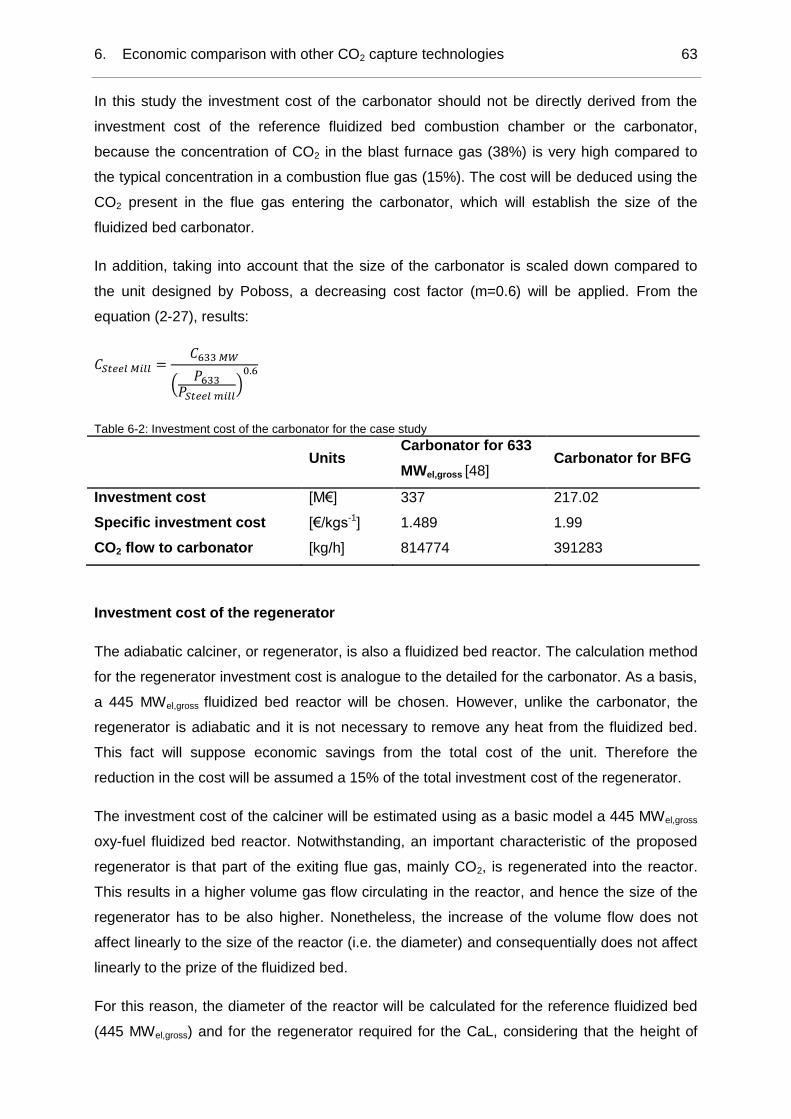
6. Economic comparison with other CO2 capture technologies 63
In this study the investment cost of the carbonator should not be directly derived from the
investment cost of the reference fluidized bed combustion chamber or the carbonator,
because the concentration of CO2 in the blast furnace gas (38%) is very high compared to
the typical concentration in a combustion flue gas (15%). The cost will be deduced using the
CO2 present in the flue gas entering the carbonator, which will establish the size of the
fluidized bed carbonator.
In addition, taking into account that the size of the carbonator is scaled down compared to
the unit designed by Poboss, a decreasing cost factor (m=0.6) will be applied. From the
equation (2-27), results:
𝐶𝑆𝑡𝑒𝑒𝑙 𝑀𝑖𝑙𝑙 =𝐶633 𝑀𝑊
(𝑃633
𝑃𝑆𝑡𝑒𝑒𝑙 𝑚𝑖𝑙𝑙)
0.6
Table 6-2: Investment cost of the carbonator for the case study
Units Carbonator for 633
MWel,gross [48] Carbonator for BFG
Investment cost [M€] 337 217.02
Specific investment cost [€/kgs-1] 1.489 1.99
CO2 flow to carbonator [kg/h] 814774 391283
Investment cost of the regenerator
The adiabatic calciner, or regenerator, is also a fluidized bed reactor. The calculation method
for the regenerator investment cost is analogue to the detailed for the carbonator. As a basis,
a 445 MWel,gross fluidized bed reactor will be chosen. However, unlike the carbonator, the
regenerator is adiabatic and it is not necessary to remove any heat from the fluidized bed.
This fact will suppose economic savings from the total cost of the unit. Therefore the
reduction in the cost will be assumed a 15% of the total investment cost of the regenerator.
The investment cost of the calciner will be estimated using as a basic model a 445 MWel,gross
oxy-fuel fluidized bed reactor. Notwithstanding, an important characteristic of the proposed
regenerator is that part of the exiting flue gas, mainly CO2, is regenerated into the reactor.
This results in a higher volume gas flow circulating in the reactor, and hence the size of the
regenerator has to be also higher. Nonetheless, the increase of the volume flow does not
affect linearly to the size of the reactor (i.e. the diameter) and consequentially does not affect
linearly to the prize of the fluidized bed.
For this reason, the diameter of the reactor will be calculated for the reference fluidized bed
(445 MWel,gross) and for the regenerator required for the CaL, considering that the height of

6. Economic comparison with other CO2 capture technologies 64
both reactors is the same. For the calculation the mass flow and density obtained in the
Aspen PlusTM simulation will be used.
Regenerator of the CaL Plant:
- Gas flow at the exit of the regenerator: 419.62 kg/s
- Density of the gas: 0.4289 kg/m³
- Velocity of the gas: 5 m/s
- Required section for the reactor: 195.6 m²→ DRegenerator: 15.78 m
Reference oxy-fuel fluidized bed reactor (445 MWel,gross):
- Gas flow at the exit of the regenerator: 203 kg/s
- Section of the reactor: 94.66 m²→ D445MW: 10.98 m
Table 6-3: Cost of the regenerator reactor
Reference 445
MWel,gross fluidized bed
Regenerator for
BFG
Investment cost [M€] 115 165.3
Flue gas at exit reactor [kg/s] 203 419.62
Diameter [m] 10.98 15.78
Specific investment cost [M€/m] 10.47 10.47
The investment cost is calculated linearly with the specific investment cost, which is defined
as the investment cost of the reactor per meter of diameter:
𝐼𝐶𝐿,𝑙𝑖𝑛𝑒𝑎𝑟 = 𝐷𝐶𝑎𝐿 ∙𝐼445𝑀𝑊
𝐷445𝑀𝑊
Finally, as it has been said before, a reduction of the investment cost of a 15% is applied
because of the avoidance of the heat removal.
𝐼𝐶𝐿, = 𝐼𝐶𝐿,𝑙𝑖𝑛𝑒𝑎𝑟 ∙ (1 − 0.15) = 140.51 𝑀€
Investment cost of the Air Separation
The oxygen required for the oxy-fuel combustion in the regenerator is provided by the Air
Separation Unit. The necessary amount of oxygen has been calculated in the simulation and
it is equal to 83.2 kg/s. The compressors of the air separation unit require electrical power for
its operation, as it has been described in chapter 2.5.1. There, it has been assumed that the
consumption of the ASU is 0.231 kWhe/kg O2, which is the value assumed by IEA in [12].
Accordingly, required electrical power by the air separation unit is 69.2 MWe.

6. Economic comparison with other CO2 capture technologies 65
The investment cost of the air separation unit will be deduced from the EU-project ENCAP
[48], where the electrical consumption and investment costs of two air separation units used
for two different oxy-fuel power plants (1000 MWel and 600 Mwel ) are presented.
Table 6-4: Cost of the ASU
O2 production Specific
consumption Consumption
Investment
Cost
[kg/s] [kWh/kgO2] [MW] [M€]
1000 MWel 176.624 0.193 124 141
600 MWel 112.51 0.185 74.88 99
ASU for CaL 83.209 0.231 69.2 95.11
From these values the coefficient “m” (or size exponent) can be calculated.
𝑚 =log (
𝐶1000 𝑀𝑊𝑒𝑙𝐶600 𝑀𝑊𝑒𝑙
)
log (𝑃1000 𝑀𝑊𝑒𝑙𝑃600 𝑀𝑊𝑒𝑙
)
The value of the size exponent “m”, for the cost evolution of the ASU is 0.497. Using this
value the investment cost of the ASU required for the CaL will be deduced for a consumption
of 69.2 MWel, resulting an investment cost of 95.11 M€.
Investment cost of the CO2 compression plant
Similar to the Air Separation Unit, the investment costs of the CO2 compression plant will be
estimated by comparison with literature data. The investment costs and the operation
information of the CO2 compression units used for the comparison are extracted from [48]
and are derived from two oxy-fuel power plants of 600 and 1000 MWel, which are
compressing a flue gas from 141.0 kg/s and 235.9 kg/s, respectively.
Table 6-5: Cost of the CO2 compression plant
Gas treated Specific
consumption Consumption
Investment
Cost
[kg/s] [kWh/kggas] [MW] [M€]
600 MWel 141.0 0.117 59.2 51
1000 MWel 235.9 0.111 94.0 67
CO2 compression
unit for CaL 201.76 0.117 84.98 63.13

6. Economic comparison with other CO2 capture technologies 66
Analog to the ASU, with these values the coefficient “m” (or size exponent) can be
calculated.
𝑚 =log (
𝐶1000 𝑀𝑊𝑒𝑙𝐶600 𝑀𝑊𝑒𝑙
)
log (𝑃1000 𝑀𝑊𝑒𝑙𝑃600 𝑀𝑊𝑒𝑙
)
The value of the size exponent “m”, for the cost evolution of the CO2 compression plant is
0.59. Using this value, the investment cost of the compression unit required for the CaL will
be deduced for a consumption of 84.98 MW, resulting in 63.13 M€.
Other investment costs
These costs make reference to all the units that have not been detailed before and comprise:
- Steam turbine and generator
- Condenser
- Cold water system
- Pipelines
- Ash system
- Fuel- and limestone system
- Electrical components
- I&C (information and communication) and peripheral components
These costs will be determined using as a reference a 445 MWel oxy-fuel power plant. As It
has been done before, a size exponent of m=0.6 will be applied for taking into account the
economy of scale. In the next table the remaining investment costs for the reference case
and the Calcium Looping facility designed for the case (368.57 MWel,gross) are summarized.
Table 6-6: Remaining investment costs
Power Investment Cost
[MW] [M€]
445 MWel power plant 445 298.8
ASU for CaL 368.57 266.86
Overview of the investment costs
Once all the investment costs have been calculated, the total investment cost for the
proposed CaL plant can be calculated and at the same time, the influence of each
component to the total amount can be seen. In Table 6-7 this is summarized.
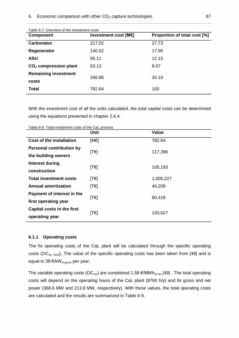
6. Economic comparison with other CO2 capture technologies 67
Table 6-7: Overview of the investment costs
Component Investment cost [M€] Proportion of total cost [%]
Carbonator 217.02 27.73
Regenerator 140.52 17.95
ASU 95.11 12.15
CO2 compression plant 63.13 8.07
Remaining investment
costs 266.86 34.10
Total 782.64 100
With the investment cost of all the units calculated, the total capital costs can be determined
using the equations presented in chapter 2.6.4.
Table 6-8: Total investment costs of the CaL process
Unit Value
Cost of the installation [M€] 782.64
Personal contribution by
the building owners [T€] 117,396
Interest during
construction [T€] 105,193
Total investment costs [T€] 1,005,227
Annual amortization [T€] 40,209
Payment of interest in the
first operating year [T€] 80,418
Capital costs in the first
operating year [T€] 120,627
6.1.1 Operating costs
The fix operating costs of the CaL plant will be calculated through the specific operating
costs (OCsp, fixed). The value of the specific operating costs has been taken from [48] and is
equal to 39 €/kWel,gross per year.
The variable operating costs (OCvar) are considered 1.58 €/MWhel,net [49] . The total operating
costs will depend on the operating hours of the CaL plant (8760 h/y) and its gross and net
power (368.6 MW and 213.8 MW, respectively). With these values, the total operating costs
are calculated and the results are summarized in Table 6-9.
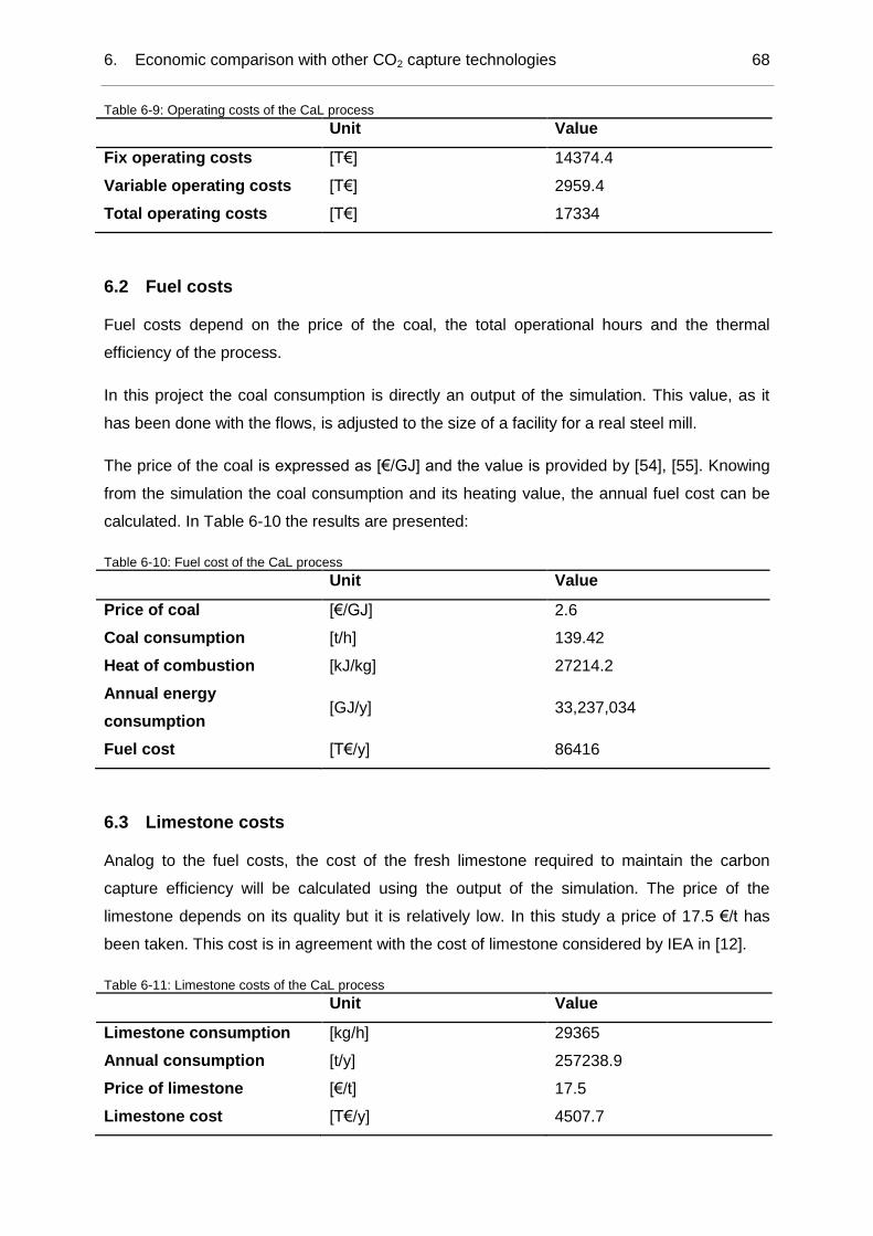
6. Economic comparison with other CO2 capture technologies 68
Table 6-9: Operating costs of the CaL process
Unit Value
Fix operating costs [T€] 14374.4
Variable operating costs [T€] 2959.4
Total operating costs [T€] 17334
6.2 Fuel costs
Fuel costs depend on the price of the coal, the total operational hours and the thermal
efficiency of the process.
In this project the coal consumption is directly an output of the simulation. This value, as it
has been done with the flows, is adjusted to the size of a facility for a real steel mill.
The price of the coal is expressed as [€/GJ] and the value is provided by [54], [55]. Knowing
from the simulation the coal consumption and its heating value, the annual fuel cost can be
calculated. In Table 6-10 the results are presented:
Table 6-10: Fuel cost of the CaL process
Unit Value
Price of coal [€/GJ] 2.6
Coal consumption [t/h] 139.42
Heat of combustion [kJ/kg] 27214.2
Annual energy
consumption [GJ/y] 33,237,034
Fuel cost [T€/y] 86416
6.3 Limestone costs
Analog to the fuel costs, the cost of the fresh limestone required to maintain the carbon
capture efficiency will be calculated using the output of the simulation. The price of the
limestone depends on its quality but it is relatively low. In this study a price of 17.5 €/t has
been taken. This cost is in agreement with the cost of limestone considered by IEA in [12].
Table 6-11: Limestone costs of the CaL process
Unit Value
Limestone consumption [kg/h] 29365
Annual consumption [t/y] 257238.9
Price of limestone [€/t] 17.5
Limestone cost [T€/y] 4507.7
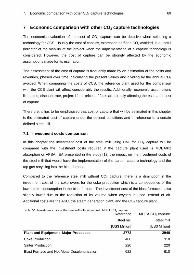
7. Economic comparison with other CO2 capture technologies 69
7 Economic comparison with other CO2 capture technologies
The economic evaluation of the cost of CO2 capture can be decisive when selecting a
technology for CCS. Usually the cost of capture, expressed as €/ton CO2 avoided, is a useful
indicator of the viability of the project when the implementation of a capture technology is
considered. However, the cost of capture can be strongly affected by the economic
assumptions made for its estimation.
The assessment of the cost of capture is frequently made by an estimation of the costs and
revenues, phased over time, calculating the present values and dividing by the annual CO2
avoided. When comparing the costs of CCS, the reference plant used for the comparison
with the CCS plant will affect considerably the results. Additionally, economic assumptions
like taxes, discount rate, project life or prices of fuels are directly affecting the estimated cost
of capture.
Therefore, it has to be emphasized that cost of capture that will be estimated in this chapter
is the estimated cost of capture under the defined conditions and in reference to a certain
defined steel mill.
7.1 Investment costs comparison
In this chapter the investment cost of the steel mill using CaL for CO2 capture will be
compared with the investment costs required if the capture plant used is MDEA/Pz
absorption or VPSA. IEA presented in the study [12] the impact on the investment costs of
the steel mill that would have the implementation of the carbon capture technology and the
top gas recycling into the blast furnace.
Compared to the reference steel mill without CO2 capture, there is a diminution in the
investment cost of the coke ovens for the coke production which is a consequence of the
lower coke consumption in the blast furnace. The investment cost of the blast furnace is also
slightly lower due to the reduction of its volume when oxygen is used instead of air.
Additional costs are the ASU, the steam generation plant, and the CO2 capture plant.
Table 7-1: Investment costs of the steel mill without and with MDEA CO2 capture
Reference
steel mill
[US$ Million]
MDEA CO2 capture
steel mill
[US$ Million]
Plant and Equipment -Major Processes 2772 2940
Coke Production 400 310
Sinter Production 220 220
Blast Furnace and Hot Metal Desulphurization 622 610

7. Economic comparison with other CO2 capture technologies 70
Basic Oxygen Steelmaking and Ladle Metallurgy 459 459
Continuous Slab Caster 195 195
Reheating Furnace & Hot Rolling Mills 450 450
Lime Production 16 16
ASU - HP 130 94
ASU - LP - 134
Power Plant 280 362
Steam Generation Plant - 90
Plant and Equipment-Material Handling &
Spare Parts 244 242
Plant and Equipment -Auxiliary, Utilities and
BOP 350 350
Site Development, Construction and Project
Engineering 562 562
Total Installed Cost 3928 4094
Contingency (5% of total investment costs) 196.4 204.7
CO2 capture & compression plant - 578
Total investment cost [US$ Million] 4124.4 4876.7
The investment costs of the steel mill with TGR-BF and using VPSA for CO2 capture have
been calculated. As it has been seen in chapter 5.4, the VPSA steel mill requires a larger
power plant compared to the MDEA steel mill. Knowing the costs of the power plant for the
MDEA steel mill the costs are scaled using a decreasing cost factor (m=0.6).
As it has been said in chapter 5.4, the VPSA steel mill does not require a steam generation
plant. Therefore, its capital cost is not considered in the total investment costs of the steel
mill. Finally, the costs of the VPSA CO2 capture and compression plant are estimated using
the specific capital cost of VPSA capture plant for a TGR-BF presented in [6].
Table 7-2: Investment costs of the steel mill with TGR-BF and VPSA CO2 capture
Cost Breakdown
VPSA CO2 capture steel mill
[US$ Million]
Plant and Equipment -Major Processes 2890.6
Coke Production 310
Sinter Production 220
Blast Furnace and Hot Metal Desulhurisation 610
Basic Oxygen Steelmaking and Ladle Metallurgy 459
Continuous Slab Caster 195
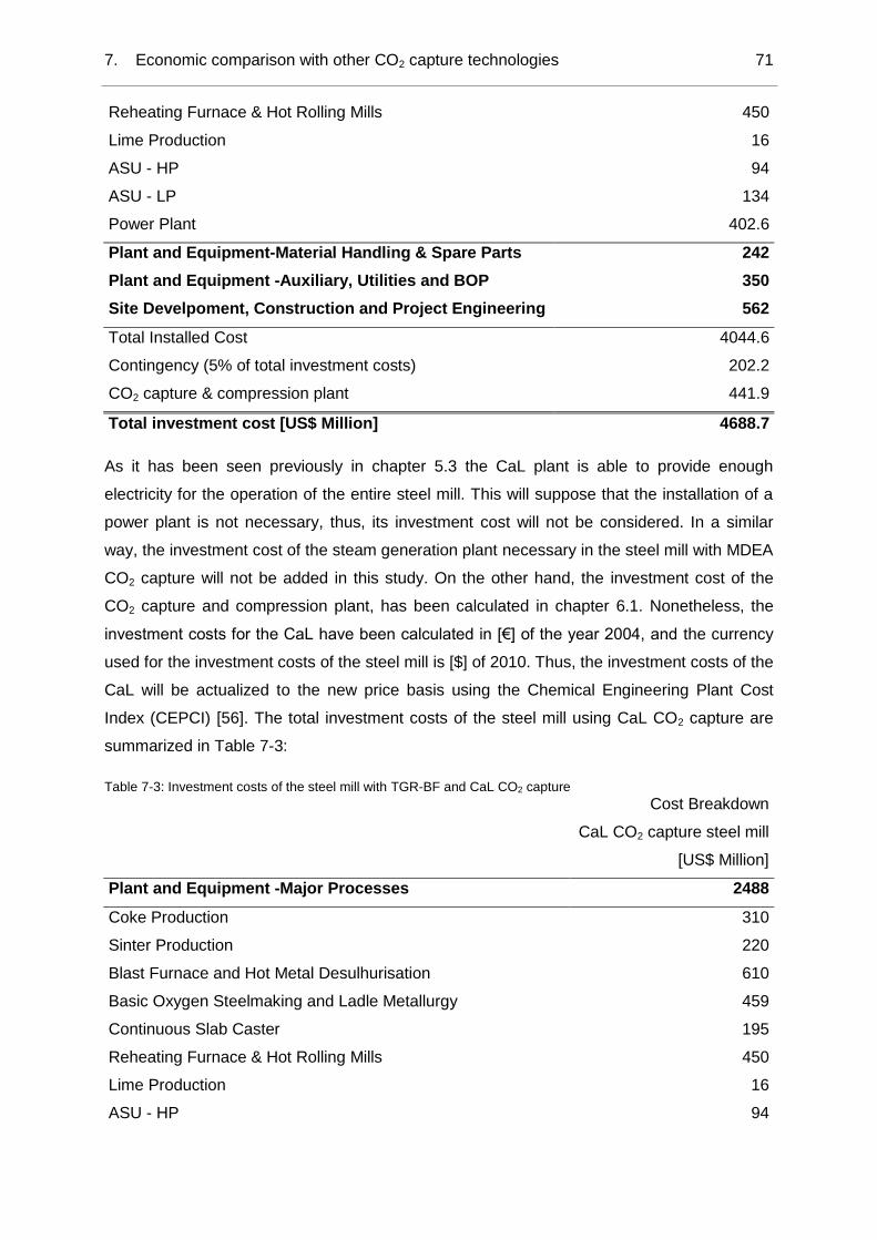
7. Economic comparison with other CO2 capture technologies 71
Reheating Furnace & Hot Rolling Mills 450
Lime Production 16
ASU - HP 94
ASU - LP 134
Power Plant 402.6
Plant and Equipment-Material Handling & Spare Parts 242
Plant and Equipment -Auxiliary, Utilities and BOP 350
Site Develpoment, Construction and Project Engineering 562
Total Installed Cost 4044.6
Contingency (5% of total investment costs) 202.2
CO2 capture & compression plant 441.9
Total investment cost [US$ Million] 4688.7
As it has been seen previously in chapter 5.3 the CaL plant is able to provide enough
electricity for the operation of the entire steel mill. This will suppose that the installation of a
power plant is not necessary, thus, its investment cost will not be considered. In a similar
way, the investment cost of the steam generation plant necessary in the steel mill with MDEA
CO2 capture will not be added in this study. On the other hand, the investment cost of the
CO2 capture and compression plant, has been calculated in chapter 6.1. Nonetheless, the
investment costs for the CaL have been calculated in [€] of the year 2004, and the currency
used for the investment costs of the steel mill is [$] of 2010. Thus, the investment costs of the
CaL will be actualized to the new price basis using the Chemical Engineering Plant Cost
Index (CEPCI) [56]. The total investment costs of the steel mill using CaL CO2 capture are
summarized in Table 7-3:
Table 7-3: Investment costs of the steel mill with TGR-BF and CaL CO2 capture
Cost Breakdown
CaL CO2 capture steel mill
[US$ Million]
Plant and Equipment -Major Processes 2488
Coke Production 310
Sinter Production 220
Blast Furnace and Hot Metal Desulhurisation 610
Basic Oxygen Steelmaking and Ladle Metallurgy 459
Continuous Slab Caster 195
Reheating Furnace & Hot Rolling Mills 450
Lime Production 16
ASU - HP 94
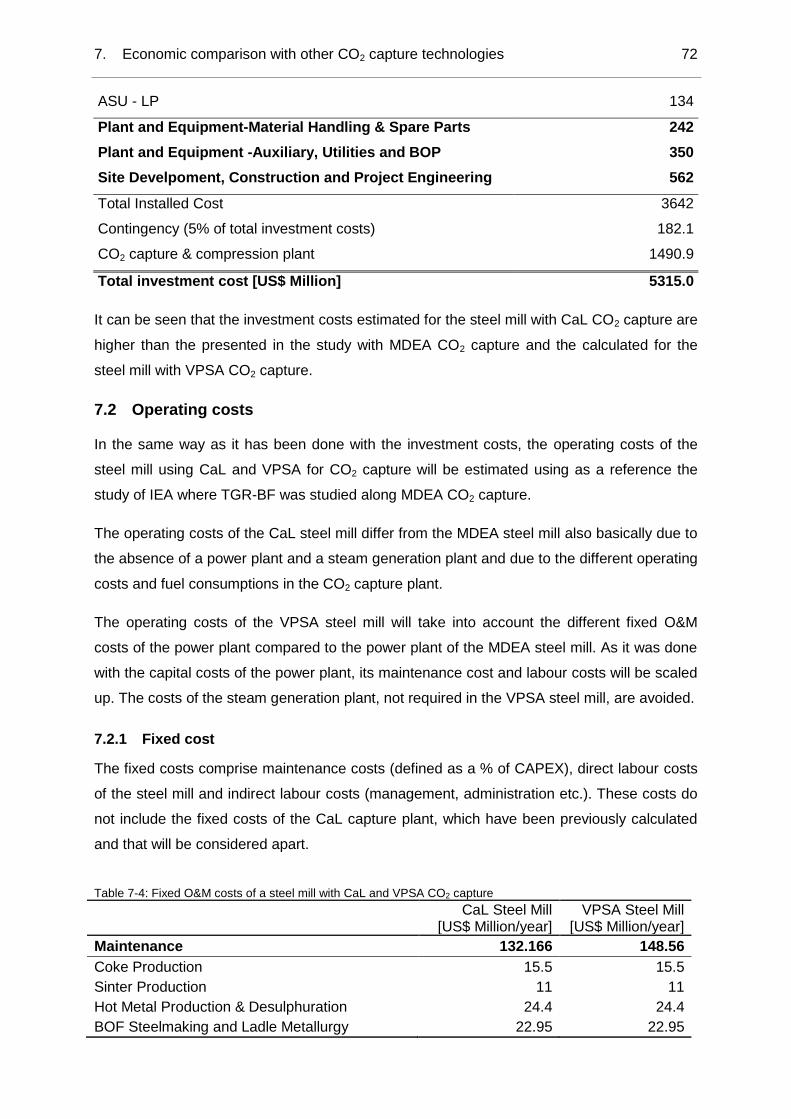
7. Economic comparison with other CO2 capture technologies 72
ASU - LP 134
Plant and Equipment-Material Handling & Spare Parts 242
Plant and Equipment -Auxiliary, Utilities and BOP 350
Site Develpoment, Construction and Project Engineering 562
Total Installed Cost 3642
Contingency (5% of total investment costs) 182.1
CO2 capture & compression plant 1490.9
Total investment cost [US$ Million] 5315.0
It can be seen that the investment costs estimated for the steel mill with CaL CO2 capture are
higher than the presented in the study with MDEA CO2 capture and the calculated for the
steel mill with VPSA CO2 capture.
7.2 Operating costs
In the same way as it has been done with the investment costs, the operating costs of the
steel mill using CaL and VPSA for CO2 capture will be estimated using as a reference the
study of IEA where TGR-BF was studied along MDEA CO2 capture.
The operating costs of the CaL steel mill differ from the MDEA steel mill also basically due to
the absence of a power plant and a steam generation plant and due to the different operating
costs and fuel consumptions in the CO2 capture plant.
The operating costs of the VPSA steel mill will take into account the different fixed O&M
costs of the power plant compared to the power plant of the MDEA steel mill. As it was done
with the capital costs of the power plant, its maintenance cost and labour costs will be scaled
up. The costs of the steam generation plant, not required in the VPSA steel mill, are avoided.
7.2.1 Fixed cost
The fixed costs comprise maintenance costs (defined as a % of CAPEX), direct labour costs
of the steel mill and indirect labour costs (management, administration etc.). These costs do
not include the fixed costs of the CaL capture plant, which have been previously calculated
and that will be considered apart.
Table 7-4: Fixed O&M costs of a steel mill with CaL and VPSA CO2 capture
CaL Steel Mill
[US$ Million/year] VPSA Steel Mill
[US$ Million/year]
Maintenance 132.166 148.56
Coke Production 15.5 15.5
Sinter Production 11 11
Hot Metal Production & Desulphuration 24.4 24.4
BOF Steelmaking and Ladle Metallurgy 22.95 22.95

7. Economic comparison with other CO2 capture technologies 73
Continuous Slab Caster 15.64 15.64
Reheating Furnace & Hot Rolling Mills 36 36
Lime Production 1.28 1.28
ASU-LP O2 Production 3.35 3.35
ASU-HP O2 Production 2.35 2.35
Power Plant - 16.09
Labour 274.71 279.1
Coke Production 17.95 17.95
Sinter Production 25.38 25.38
Hot Metal Production & Desulphuration 30.17 30.17
BOF Steelmaking and Ladle Metallurgy 37.22 37.22
Continuous Slab Caster 33.84 33.84
Reheating Furnace & Hot Rolling Mills 45.16 45.16
Lime Production 3.2 3.2
ASU-LP O2 Production 3.29 3.29
ASU-HP O2 Production 2.35 2.35
Power Plant - 4.39
Indirect Labour 76.14 76.14
Total Fixed O&M Cost [US$ Million/year] 406.87 427.65
7.2.2 Variable cost
The most important variable costs are the fuel required in the steel mill and the iron ore. The
consumption points of natural gas in the MDEA steel mill were the following:
- Power plant: 3647 MJ/t HRC
- Steam generation plant: 653 MJ/t HRC
- Blast furnace process gas heaters: 745 MJ/t HRC
This natural gas consumption represented in the steel mill with MDEA CO2 capture an
expense of 197.173 M$/year.
The consumption of natural gas for the steel mill with VPSA CO2 capture will be recalculated.
The natural gas combined cycle generates the electricity calculated in chapter 5.4. Using the
same efficiency (56.6%) the fuel consumption in the power plant is calculated. In this power
plant, besides natural gas, Basic Oxygen Furnace Gas will be burned. As it was explained in
chapter 5.2.2, the steam generation plant of the MDEA steel mill burned this gas together
with natural gas. Since the steam generation plant is not required in the VPSA steel mill, this
gas is available and will be used in the power plant to reduce the total natural gas
consumption, as it is shown in Table 7-5.

7. Economic comparison with other CO2 capture technologies 74
Table 7-5: Fuel balance in the VPSA steel mill
MJ/t HRC
Energy consumption in power plant 4356.2
Energy from Basic Oxygen Furnace Gas 660
Natural Gas for power plant 3696.2
Natural gas for process gas heaters 745
Total consumption of Natural Gas 4441.2
This natural gas consumption represented in the steel mill with VPSA CO2 capture an
expense of 173.56 M$/year.
For the proposed steel mill with CaL the operating costs are considerably reduced compared
to the MDEA CO2 capture steel mill because as it has been seen in chapter 5.3, natural gas
is not necessary in the power plant or for steam production. Additionally, the heating of the
process gas, before the reinjection into the blast furnace is not done with natural gas, but as
it has been described in chapter 3.4.
Other significant costs include ferroalloys and scrap, which are required in the production of
steel in the basic oxygen furnace or in secondary metallurgy. The cost of the limestone
required in the CaL is included in the Fluxes cost of the steel mill (which makes reference to
limestone and other elements required for the steel mill operation). Miscellaneous expense
includes services related to logistics, engineering, analysis, etc… Finally, the disposal of the
MDEA sludge is also an extra cost when MDEA capture is considered but avoided in the CaL
and VPSA steel mills.
As it has been done with the fixed operating costs, the variable costs of the CaL capture
plant are not included in the following table and will be presented together with the VPSA
capture plant O&M costs as a cost apart, in Table 7-7. Regarding the O&M cost of the VPSA
CO2 capture plant, equals to 20.9 M$/year, it has been considered that it is equal to 6% of
the capital cost of the VPSA plant [55].
Table 7-6: Variable O&M costs of steel mill with CaL and VPSA CO2 capture
CaL Steel Mill
[US$ Million/year] VPSA Steel Mill
[US$ Million/year]
Fuel and Reductant 479.66 538.56
Hard coking coal 182.43 182.43
Semi-soft coking coal 93.13 93.13
PCI coal 89.45 89.45
Natural Gas - 173.56
Coal for CaL 114.66 -
Iron Ore (Fines , Lumps and Pellets) 492.29 492.29

7. Economic comparison with other CO2 capture technologies 75
Purchased Scrap & Ferroalloys 218.23 218.23
Fluxes (Limestone, Quartzite, Olivine…) 46.07 40.09
Consumables & Other Utilities 41.76 50.52
Refractories 22.60 22.60
Electrode (Ladle Metallurgy) 5.29 5.29
Casting Power (Continuous Caster) 2.26 2.26
Works Back Up Rolls (Hot Rolling Mill) 9 9
Banding (Hot Rolling Mills) 0.36 0.36
Water 2.25 2.25
Chemicals and consumables of Power Plant - 8.76
Miscellaneous Expense 67.2 67.2
Miscellaneous works Expense 48.07 48.07
Other Misc. OPEX (environmental clean-up) 10.97 10.97
Slag Processing 3.83 3.83
Disposal and Landfill 4.33 4.33
Total Variable O&M Cost [US$ Million/year] 1345.20 1406.89
Table 7-7: Operating Costs of CaL and VPSA CO2 capture plant
O&M costs CO2 capture plant [US$ Million/year]
CaL capture plant O&M costs 25.709
VPSA capture plant O&M costs 20.90
The total operating and maintenance costs of the steel mill, presented in Table 7-8, are
calculated by adding the total variable costs to the total fixed costs of the steel mill and
including the operating costs of the CO2 capture plant.
Table 7-8: Total annual O&M cost of the steel mill with CaL and VPSA CO2 capture plant
CaL Steel Mill
[US$ Million/year] VPSA Steel Mill
[US$ Million/year]
Total Fixed O&M Cost steel mill 406.87 427.65 Total Variable O&M Cost steel mill 1345.20 1406.89 O&M Cost CO2 capture plant 25.709 20.9
Total annual O&M Cost 1777.78 1855.44
In Table 7-9 the comparison of the costs of the entire steel mill for the four different cases is
shown: the reference steel mill without CO2 capture and the steel mills with TGR-BF and CO2
capture (MDEA, VPSA and CaL).
It can be noted that the operating costs of the CaL steel mill are slightly lower than the
operating costs of the reference steel mill but considerably lower than the operating costs of
MDEA or VPSA steel mills. This fact is mainly consequence of the avoided natural gas, even
though the coal consumption in the CaL is significant. Therefore, the fuel and reductant costs
of the CaL steel mill are lower. Furthermore, the avoidance of the steam generation and the
power plant lead to important savings in maintenance and labour. Finally, the increase in the

7. Economic comparison with other CO2 capture technologies 76
miscellaneous expense & other costs of both steel mills with CO2 capture in relation to the
reference steel mill is caused because the revenues from by–products sale are included in
these costs, which dropped because less argon (see section 2.5.1) and coke by-products are
sold.
Table 7-9: Comparison of the investment and operating costs of the different steel mills
Reference Steel
Mill
MDEA Steel
Mill
VPSA
Steel Mill
CaL Steel
Mill
Total Investment cost
[US$ Million] 4124.4 4876.7 4688.7 5315
Operating costs Steel mill
[US$ Million/year] 1781.80 1882.84 1855.44 1777.78
Maintenance 142.00 163.63 148.56 132.17
Labour 280.72 281.66 279.10 274.71
Fuel and Reductant 483.94 562.21 538.56 479.66
Iron Ore 492.05 492.29 492.29 492.29
Purchased Scrap&Ferroalloys 218.23 218.23 218.23 218.23
Fluxes 44.65 40.09 40.09 46.07
Consumables & Other Utilities 49.78 57.08 50.52 41.76
Miscellanous Expense & Other 70.43 67.64 67.2 67.2
CaL CO2 capture plant - - - 25.71
VPSA CO2 capture plant - - 20.90 -
7.3 Cost of steel production
The cost of the steel production is calculated for the reference steel mill and subsequently,
for the steel mill with MDEA, with VPSA and with CaL. The cost of steel production is
calculated as it has been explained in chapter 2.6.6. The results, presented in Table 7-10,
show that the costs of steel production from the steel mills with TGR-BF and CO2 capture are
higher than in the case of the reference steel mill.
Table 7-10: Cost of steel production for the different steel mills
Unit
Reference
Steel Mill
MDEA
Steel Mill
VPSA
Steel Mill
CaL
Steel Mill
Capital Recovery
Factor CRF [ ] 0.110 0.110 0.110 0.110
Present Value of
Total Costs PVTC [M$] 20529.45 22369.43 21932.43 21853.85

7. Economic comparison with other CO2 capture technologies 77
Levelized Total
Annual Costs LAN [M$] 2261.69 2464.40 2416.25 2407.60
Cost of steel
production CHRC [$/t HRC] 565.42 616.10 604.06 601.90
Table 7-11 shows the breakdown of the cost of steel production. Since the annual steel
production, the life of the project and the discount rate in the three cases are the same, the
breakdown of the costs of production and its total cost, are in accordance with the operation
and capital costs shown in Table 7-9.
Table 7-11: Breakdown of the total cost of steel production
Reference SM
[US$/t HRC]
MDEA SM
[US$/t HRC]
VPSA SM
[US$/t HRC]
CaL SM
[US$/t HRC]
Capital Costs 119.97 140.71 135.53 152.78
Fuel & Reductant 120.98 140.55 134.64 119.91
Iron Ore 123.01 123.07 123.07 123.07
Scrap & Ferroalloy 54.56 54.56 54.56 54.56
Fluxes 11.16 10.02 10,02 11.52
Consumables 12.45 14.27 12.63 10.44
Labour 70.18 70.42 69.77 68.68
Maintenance 35.50 40.91 41.82 37.72
Miscellaneous & Other 17.61 21.59 16.8 16.80
CaL O&M costs - - - 6.43
VPSA O&M costs - - 5.22 -
Total [US$/t HRC] 565.42 616.10 604.06 601.90
The influence of the different costs to the total cost of steel production is shown for the
different cases in Figure 7-1. It can be observed that the influence of the capital cost to the
total cost of steel production is for the case of the CaL higher, due to its high capital costs but
lower operating costs. In the same way, the influence of the fuel and reductant cost to the
total cost is lower, consequence of the avoidance of natural gas.

7. Economic comparison with other CO2 capture technologies 78
Figure 7-1: Cost of steel production for the different steel mills
Once the costs of steel production have been calculated, and knowing the CO2 emissions of
the different steel mills (see chapter 5.5), the cost of CO2 avoidance can be calculated with
the formula (2-33).
Table 7-12: Cost of CO2 avoidance for the steel mills with CaL, VPSA and MDEA CO2 capture
CHRC
CO2
emission
CO2
avoided
CO2
avoidance
cost
[$/t HRC] [kg/t HRC] [%] [$/t CO2]
Reference Steel Mill 565.42 2090.14 - -
Steel Mill with TGR-BF &
MDEA CO2 capture 616.10 1114.75 46.7% 51.96
Steel Mill with TGR-BF &
VPSA CO2 capture 604.06 879.67 58.0% 31.82
Steel Mill with TGR-BF & CaL
CO2 capture 601.90 633.89 69.7% 24.98
The cost of CO2 avoidance calculated for the steel mill with TGR-BF along CaL for the CO2
separation is 24.98 US$/t CO2. This cost is considerably lower than the cost of capture for
the steel mill with MDEA/Pz capture due to the lower cost of steel production and, especially,
due to the substantially lower CO2 emissions.
0.00
100.00
200.00
300.00
400.00
500.00
600.00
700.00
Reference SM MDEA SM VPSA SM CaL SM
VPSA plant O&M Costs
CaL plant O&M Costs
Miscellaneous & Other
Maintenance
Labour
Consumables
Fluxes
Scrap & Ferroalloy
Iron Ore
Fuel & Reductant
Capital Costs
8. Conclusions 79
8 Conclusions
In this project the use of Calcium Looping for CO2 capture in the Top Gas Recycling Blast
Furnace was studied. A simulation of the Calcium Looping treating the blast furnace gas
defined by ULCOS was carried out in Aspen Plus using as boundary conditions previous
experimental results of a 200 kWth DBF pilot plant. The main results of the simulation were
the consumptions of coal, oxygen and limestone and the energy that could be recovered
from the CaL for steam production. The treatment of the process gas (CO2-lean) was also
simulated, i.e. heating of the gas previous reinjection in to the blast furnace.
In the second part of the project, CaL was compared with VPSA, which was the capture
technology proposed by ULCOS, and with amines adsorption (MDEA/Pz) that was presented
by the IEAGHG. The operation of a steel mill is different depending on the CO2 capture
technology employed. The differences are a result of the different energy requirements of the
CO2 capture technologies (steam, electricity or coal) and due to the fact that CaL, unlike the
other technologies, is able to generate electricity.
The energy consumptions of the steel mill using VPSA and CaL were calculated using a
study of the IEA where TGR-BF was implemented in a steel mill with MDEA for capture as a
reference. Remarkable is that the electricity produced in the CaL was found to be enough to
meet the electricity demand of the steel mill. Therefore, no power plant is required in the CaL
steel mill.
Unlike the MDEA technology, the CaL and the VPSA capture plants do not require steam for
the capture. Thus, the steam demand of the steel mill is substantially lower than the steel mill
with MDEA and the Steam Generation Plant, necessary in the steel mill with MDEA, can be
avoided in both cases.
In the VPSA CO2-capture plant steam is avoided but the electricity consumption is higher
than the MDEA. Therefore, the total electricity demand of the steel mill is increased and the
power plant required for the VPSA steel mill has been resized to meet the higher demand.
The direct consequence of the different conceptions of the steel mill is the difference in the
CO2 emissions. The steel mill with TGR-BF and using MDEA for capture reduces the CO2
emissions by 46.6% compared to the steel mill without capture. The emissions of the VPSA
steel mill have been calculated taking into account the avoidance of the steam generation
plant but a higher CO2 emission in the power plant (which has a larger electricity generation).
The CO2 emissions for this case were reduced by 58%. In the CaL steel mill, the CO2
emissions were reduced by almost 70%. Calcium Looping generates electricity without
emissions to the atmosphere since CO2 is generated in a pure flow that can be stored. In
8. Conclusions 80
addition, unlike in the other two methods, CaL CO2 capture technology does not have
associated extra CO2 emissions (MDEA requires steam and VPSA electricity that are
produced by a power plant generating CO2).
In the last part of the project the cost of the CaL was estimated and an economical
comparison of the three capture methods was done. The investment costs for the steel mill
using CaL for capture resulted higher than for the other capture technologies due to the
higher cost of the CO2 capture plant. However, the operating costs were lower. The
avoidance of the power plant and steam generation plant leads to lower maintenance, labour
and other costs. Moreover, the CaL steel mill does not require natural gas (which is burned in
the other steel mills) and, although the coal consumption is high, the fuel costs of the steel
mill are reduced.
The cost of steel production was slightly lower for CaL than for other cases with CO2 capture.
This fact, together with a higher rate of CO2 avoided, results in lower cost of CO2 avoidance
(approximately 25 $/t CO2). It has to be remarked that these costs are the cost of CO2
avoidance for this reference steel mill that is producing its own electricity in the boundary
limits of the plant and under the economic assumptions considered in the project.
The utilization of CaL Process for production of hydrogen through the Adsorption-Enhanced-
Reforming of the blast furnace gas was not studied in depth in this project. The CaL has
been considered only as a CO2 capture method, keeping the same conditions and
composition of the process gas as it had been done with other capture technologies to be
able to compare them. However, this could be a field of study for future projects. This
possibility is presented in Appendix 9.1.
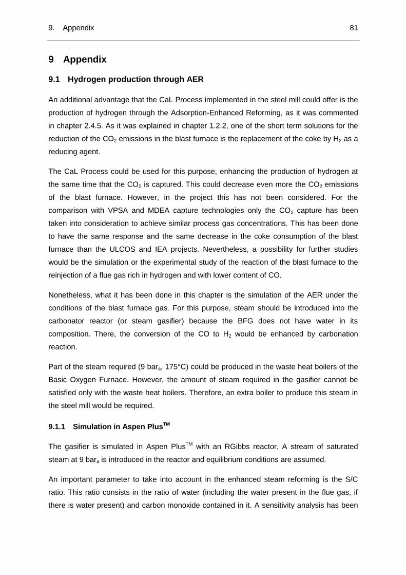
9. Appendix 81
9 Appendix
9.1 Hydrogen production through AER
An additional advantage that the CaL Process implemented in the steel mill could offer is the
production of hydrogen through the Adsorption-Enhanced Reforming, as it was commented
in chapter 2.4.5. As it was explained in chapter 1.2.2, one of the short term solutions for the
reduction of the CO2 emissions in the blast furnace is the replacement of the coke by H2 as a
reducing agent.
The CaL Process could be used for this purpose, enhancing the production of hydrogen at
the same time that the CO2 is captured. This could decrease even more the CO2 emissions
of the blast furnace. However, in the project this has not been considered. For the
comparison with VPSA and MDEA capture technologies only the CO2 capture has been
taken into consideration to achieve similar process gas concentrations. This has been done
to have the same response and the same decrease in the coke consumption of the blast
furnace than the ULCOS and IEA projects. Nevertheless, a possibility for further studies
would be the simulation or the experimental study of the reaction of the blast furnace to the
reinjection of a flue gas rich in hydrogen and with lower content of CO.
Nonetheless, what it has been done in this chapter is the simulation of the AER under the
conditions of the blast furnace gas. For this purpose, steam should be introduced into the
carbonator reactor (or steam gasifier) because the BFG does not have water in its
composition. There, the conversion of the CO to H2 would be enhanced by carbonation
reaction.
Part of the steam required (9 bara, 175°C) could be produced in the waste heat boilers of the
Basic Oxygen Furnace. However, the amount of steam required in the gasifier cannot be
satisfied only with the waste heat boilers. Therefore, an extra boiler to produce this steam in
the steel mill would be required.
9.1.1 Simulation in Aspen PlusTM
The gasifier is simulated in Aspen PlusTM with an RGibbs reactor. A stream of saturated
steam at 9 bara is introduced in the reactor and equilibrium conditions are assumed.
An important parameter to take into account in the enhanced steam reforming is the S/C
ratio. This ratio consists in the ratio of water (including the water present in the flue gas, if
there is water present) and carbon monoxide contained in it. A sensitivity analysis has been
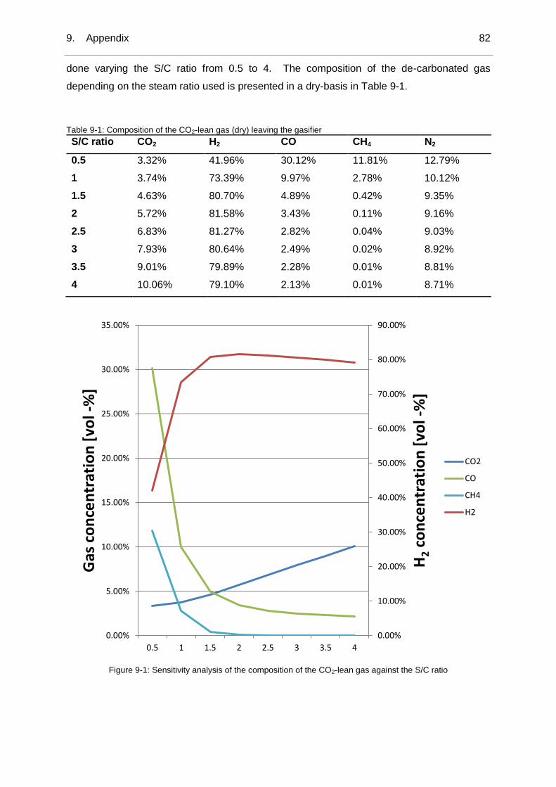
9. Appendix 82
done varying the S/C ratio from 0.5 to 4. The composition of the de-carbonated gas
depending on the steam ratio used is presented in a dry-basis in Table 9-1.
Table 9-1: Composition of the CO2-lean gas (dry) leaving the gasifier
S/C ratio CO2 H2 CO CH4 N2
0.5 3.32% 41.96% 30.12% 11.81% 12.79%
1 3.74% 73.39% 9.97% 2.78% 10.12%
1.5 4.63% 80.70% 4.89% 0.42% 9.35%
2 5.72% 81.58% 3.43% 0.11% 9.16%
2.5 6.83% 81.27% 2.82% 0.04% 9.03%
3 7.93% 80.64% 2.49% 0.02% 8.92%
3.5 9.01% 79.89% 2.28% 0.01% 8.81%
4 10.06% 79.10% 2.13% 0.01% 8.71%
Figure 9-1: Sensitivity analysis of the composition of the CO2-lean gas against the S/C ratio
0.00%
10.00%
20.00%
30.00%
40.00%
50.00%
60.00%
70.00%
80.00%
90.00%
0.00%
5.00%
10.00%
15.00%
20.00%
25.00%
30.00%
35.00%
0.5 1 1.5 2 2.5 3 3.5 4
H2 c
on
cen
trat
ion
[vo
l -%
]
Gas
co
nce
ntr
atio
n [
vol -
%]
CO2
CO
CH4
H2

9. Appendix 83
It can be observed that for a certain point (approx. S/C = 2) the maximum conversion of CO
towards H2 formation would be achieved.
Figure 9-2: Aspen Plus sensitivity analysis. Molar flow of CO at the exit of the gasifier against S/C ratio
Figure 9-3: Aspen Plus sensitivity analysis. Molar flow of hydrogen at the exit of the gasifier against S/C ratio
Sensitivity S-1 Results Summary
SC
KM
OL/
SE
C
0,5 1,0 1,5 2,0 2,5 3,0 3,5 4,0
5,e
-004
1,e
-003 COOUT
Sensitivity S-1 Results Summary
SC
KM
OL/
SE
C
0,5 1,0 1,5 2,0 2,5 3,0 3,5 4,0
0,0
03
0,0
04
0,0
05
0,0
06
0,0
07
0,0
08
0,0
09
H2OUT

9. Appendix 84
9.2 Flow sheets of Aspen PlusTM simulation
REGENER
DECOMPCYCLONE
BOT T OM
CYCLONE1
H2OSEP2
PURGE
CARBONAT
BFG
SOLIDS2
EXIT
LEAN-CO2
OXYGENCOMBOUT
SOLIDS1
HIGH-CO2
PURGE
CACO3
COALCOALDEC
Q-DECOMP
T O-LOOP
ASH
CAO
H2O-2
HIGH-DRY
QGASIFIC
Q
Figure 9-4: Aspen PlusTM
flow sheet of the basic simulation using RStoic carbonator reactor

Appendix 85
REGENER
DECOMPCYCLONE
BOTTOM
CYCLONE1
H2OSEP
PURGE
SPLIT-BFHEATER8
HEATER9
HEATER3
HEATER5
HEATER4
HEATER2
COMBUSTO
SPLITCOM
CARBONAT
CO2-SPLI
HEATER1
SOLIDS1
COALDEC
Q-DECOMP
CACO3
CO2-LOOP
OXYGEN
COMBOUT
COAL
HIGH-CO2
SOLIDS2ASH
CAO
EXIT
LEAN-CO2H2O
HIGH-DRY
PURGE
TO-LOOP
TO-TUYER
TO-SHAFT
TO-HEART
SHAFT
Q89
HEARTH
CO2COLD2
QS2
BFG
Q45
BFGHOT
CO2COLD5
CO2COLD3
Q12
HOT-LEAN
AIR
TO-COMBPRODUCTS
QS1
Figure 9-5: Aspen PlusTM
flow sheet of the simulation with heat integration. Scenario with CO2 recirculation into the regenerator

Appendix 86
GASIFICA
REGENERDECOMP
CYCLONE
ASHSEP
CYCLONE1
H2OSEPH2OSEP2
PURGE
BF G
SOLIDS2
EXIT
LEAN-CO2
OXYGENCOMBOUT
SOLIDS1
HIGH-CO2
PURGE
CACO3
COALCOALDEC
Q-DECOMP
TO-LOOP ASH
CAO
LEAN-DRY
H2OH2O-2
HIGH-DRY
QS1
Q
ST EAM
Figure 9-6: Aspen PlusTM
flow sheet of the simulation introducing steam into the gasifier

Appendix 87
9.3 Operating costs of the reference steel mill
The breakdown of the most important costs of the reference steel mill without CO2 capture
and with TGR-BF and MDEA adsorption that differ from the CaL/VPSA steel mill will be
presented in the following annex.
9.3.1 Maintenance costs
Table 9-2: Maintenance costs of the reference steel mill without capture and with MDEA capture. Table D-5 [12]
9.3.2 Labour costs
Table 9-3: Labour costs of the reference steel mill without capture and with MDEA capture. Table D-6 [12]
The indirect labour for both steel mills is equal to US$ 76.14 Million per year.
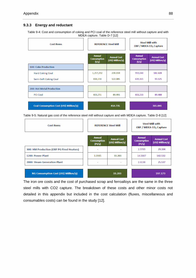
Appendix 88
9.3.3 Energy and reductant
Table 9-4: Cost and consumption of coking and PCI coal of the reference steel mill without capture and with MDEA capture. Table D-7 [12]
Table 9-5: Natural gas cost of the reference steel mill without capture and with MDEA capture. Table D-8 [12]
The iron ore costs and the cost of purchased scrap and ferroalloys are the same in the three
steel mills with CO2 capture. The breakdown of these costs and other minor costs not
detailed in this appendix but included in the cost calculation (fluxes, miscellaneous and
consumables costs) can be found in the study [12].

Appendix 89
9.4 Chemical Engineering Plant Cost Index (CEPCI)
The indexes used for the updating of the cost of the units are presented in Table 9-6.
Table 9-6: CEPCI index [56]
2002 395.6
2003 402
2004 444.2
2005 468.2
2006 499.6
2007 525.4
2008 575.4
2009 521.9
2010 550.8
2011 585.7
2012 584.6
2013 567.3
2014 575.7

10. References 90
10 References
[1] M. T. Ho, A. Bustamante, and D. E. Wiley, “Comparison of CO2 capture economics for iron and steel mills,” Int. J. Greenh. Gas Control, vol. 19, pp. 145–159, 2013.
[2] M. Halmann and A. Steinfeld, “Reforming of Blast Furnace Gas with Methane, Steam, and Lime for Syngas Production and CO 2 Capture: A Thermodynamic Study,” Miner. Process. Extr. Metall., vol. Review 36:, no. November 2014, p. 130411180227007, 2015.
[3] Worldsteel Association, “World Steel in Figures,” p. 29, 2014.
[4] M. Gazzani, M. Romano, and G. Manzolini, “Application of Sorption Enhanced Water Gas Shift for Carbon Capture in Integrated Steelworks,” Energy Procedia, vol. 37, pp. 7125–7133, 2013.
[5] J. Van Der Stel, D. Sert, A. Hirsch, N. Eklund, and L. S. Ökvist, “Top Gas Recycle Blast Furnace developments for low CO2 ironmaking,” 2011.
[6] M. T. Ho, A. Bustamante, and D. E. Wiley, “Comparison of CO2 Capture Economics for Iron and Steel Mills,” pp. 1–30, 2012.
[7] J. V. D. Stel, Hattink M., Sert D., M. Zagaria, N. Eklund, M. Pettersson, L. Sundqvist, B. S. Mefos, C. Feilmayr, K. Kinnunen, J. P. S. Wurth, and W. Küttner, “Developments of the ULCOS Low CO2 Blast Furnace Process at the LKAB Experimental BF in Luleå Abstract Key Words History of Recycling of Blast Furnace Top Gas,” no. July, pp. 1–8, 2011.
[8] C. Wang, “Utilization of biomass for blast furnace in Sweden,” pp. 1–97, 2013.
[9] J. V. D. Stel, M. Hattink;, C. Zeilstra;, and G. Louwerse, EUR 26414-ULCOS top gas recycling blast furnace process (ULCOS TGRBF). 2014.
[10] J. Van Der Stel, “Development of ULCOS-Blast Furnace : Working toward technology demonstration,” Iron steel Ind. CCUS Process Integr. Work., no. November, 2013.
[11] J.-P. Birat, Developments and Innovation in Carbon Dioxide (Co2) Capture and Storage Technology. Elsevier, 2010.
[12] S. (IEAGHG) Santos, “Iron and Steel CCS Study (Techno-Economics Integrated Steel Mill),” Int. Energy Agency, vol. 04, 2013.
[13] A. Arasto, E. Tsupari, J. Kärki, E. Pisilä, and L. Sorsamäki, “Post-combustion capture of CO 2 at an integrated steel mill – Part I : Technical concept analysis,” Int. J. Greenh. Gas Control, vol. 16, pp. 271–277, 2013.
[14] G. Wingrove, D. Satchell, B. Keenan, and C. Van Aswegen, “Developments in Ironmaking and Opportunities for Power Generation,” 1999 Gasif. Technol. Conf., pp. 1–19, 1999.
[15] M. Geerdes, H. Toxopeus, and C. Van der Vliet, Modern Blast Furnace Ironmaking: An Introduction, 2nd ed. Amsterdam: IOS Press BV, 2009.

10. References 91
[16] J. G. Peacey and W. G. Davenport, El Alto horno de hierro. México D.F. [etc.] : Limusa, 1986.
[17] J. J. Moore, “7 – Metal Extraction Processes,” in Chemical Metallurgy, 1990, pp. 243–309.
[18] G. Danloy, J. Van Der Stel, and P. Schmöle, “Heat and mass balances in the ULCOS Blast Furnace,” Proc. 4th Ulcos Semin., no. October, p. 3, 2008.
[19] Z. Liu, C. a. Grande, P. Li, J. Yu, and A. E. Rodrigues, “Multi-bed vacuum pressure swing adsorption for carbon dioxide capture from flue gas,” Sep. Purif. Technol., vol. 81, no. 3, pp. 307–317, 2011.
[20] M. T. Ho, G. W. Allinson, and D. E. Wiley, “Reducing the Cost of CO2 Capture from Flue Gases Using Pressure Swing Adsorption,” Ind. Eng. Chem. Res., vol. 47, pp. 4883–4890, 2008.
[21] T. Shimizu, T. Hirama, H. Hosoda, K. Kitano, M. Inagaki, and K. Tejima, “A Twin Fluid-Bed Reactor for Removal of CO2 from Combustion Processes,” Chem. Eng. Res. Des., vol. 77, no. 1, pp. 62–68, Jan. 1999.
[22] S. Sivalingam, “CO2 separation by calcium looping from full and partial oxidation processes,” 2013.
[23] H. Dieter, A. R. Bidwe, G. Varela-Duelli, A. Charitos, C. Hawthorne, and G. Scheffknecht, “Development of the calcium looping CO2 capture technology from lab to pilot scale at IFK, University of Stuttgart,” Fuel, vol. 127, pp. 23–37, 2014.
[24] C. Hawthorne, M. Trossmann, P. Galindo Cifre, A. Schuster, and G. Scheffknecht, “Simulation of the carbonate looping power cycle,” Energy Procedia, vol. 1, no. 1, pp. 1387–1394, 2009.
[25] A. Charitos, C. Hawthorne, a. R. Bidwe, S. Sivalingam, A. Schuster, H. Spliethoff, and G. Scheffknecht, “Parametric investigation of the calcium looping process for CO2 capture in a 10 kWth dual fluidized bed,” Int. J. Greenh. Gas Control, vol. 4, no. 5, pp. 776–784, 2010.
[26] A. Charitos, N. Rodriguez, C. Hawthorne, M. Alonso, M. Zieba, B. Arias, G. Kopanakis, G. Scheffknecht, and J. C. Abanades, “Experimental Validation of the Calcium Looping CO 2 Capture Process with Two Circulating Fluidized Bed Carbonator Reactors,” Ind. Eng. Chem. Res., vol. 50, pp. 9685–9695, 2011.
[27] C. Hawthorne, N. Poboss, H. Dieter, A. Gredinger, M. Zieba, and G. Scheffknecht, “Operation and results of a 200-kWth dual fluidized bed pilot plant gasifier with adsorption-enhanced reforming,” Biomass Convers. Biorefinery, pp. 217–227, 2012.
[28] N. H. Florin and A. T. Harris, “Enhanced hydrogen production from biomass with in situ carbon dioxide capture using calcium oxide sorbents,” Chem. Eng. Sci., vol. 63, pp. 287–316, 2008.
[29] S. Koppatz, C. Pfeifer, R. Rauch, H. Hofbauer, T. Marquard-Moellenstedt, and M. Specht, “H2 rich product gas by steam gasification of biomass with in situ CO2 absorption in a dual fluidized bed system of 8 MW fuel input,” Fuel Process. Technol., vol. 90, no. 7–8, pp. 914–921, 2009.

10. References 92
[30] B. R. Stanmore and P. Gilot, “Review-calcination and carbonation of limestone during thermal cycling for CO2 sequestration,” Fuel Process. Technol., vol. 86, pp. 1707–1743, 2005.
[31] D. P. Harrison, “Calcium enhanced hydrogen production with CO2 capture,” Energy Procedia, vol. 1, no. 1, pp. 675–681, 2009.
[32] M. Alonso, N. Rodríguez, B. González, G. Grasa, R. Murillo, and J. C. Abanades, “Carbon dioxide capture from combustion flue gases with a calcium oxide chemical loop. Experimental results and process development,” Int. J. Greenh. Gas Control, vol. 4, pp. 167–173, 2010.
[33] M. Alonso, N. Rodriguez, G. Grasa, and J. C. Abanades, “Modelling of a fluidized bed carbonator reactor to capture CO2 from a combustion flue gas,” Chem. Eng. Sci., vol. 64, pp. 883–891, 2009.
[34] L. M. Romeo, J. C. Abanades, J. M. Escosa, J. Paño, A. Giménez, A. Sánchez-Biezma, and J. C. Ballesteros, “Oxyfuel carbonation/calcination cycle for low cost CO2 capture in existing power plants,” Energy Convers. Manag., vol. 49, pp. 2809–2814, 2008.
[35] J. C. Abanades, E. S. Rubin, and E. J. Anthony, “Sorbent Cost and Performance in CO2 Capture Systems,” pp. 3462–3466, 2004.
[36] T. Pröll and H. Hofbauer, “H2 rich syngas by selective CO2 removal from biomass gasification in a dual fluidized bed system - Process modelling approach,” Fuel Process. Technol., vol. 89, no. 11, pp. 1207–1217, 2008.
[37] N. Armbrust, G. Duelli, H. Dieter, and G. Scheffknecht, “Calcium looping cycle for hydrogen production from biomass gasification syngas-experimental investigation at 20 kWth dual fluidized bed facility,” 2014.
[38] T. Weimer, R. Berger, C. Hawthorne, and J. C. Abanades, “Lime enhanced gasification of solid fuels: Examination of a process for simultaneous hydrogen production and CO2 capture,” Fuel, vol. 87, pp. 1678–1686, 2008.
[39] F. Donat, N. H. Florin, E. J. Anthony, and P. S. Fennell, “Influence of high-temperature steam on the reactivity of CaO sorbent for CO 2 capture,” Environ. Sci. Technol., vol. 46, pp. 1262–1269, 2011.
[40] J. C. Abanades and D. Alvarez, “Conversion limits in the reaction of CO2 with lime,” Energy and Fuels, vol. 17, no. 2, pp. 308–315, 2003.
[41] A. Coppola, F. Montagnaro, P. Salatino, and F. Scala, “Attrition of limestone during CO2 capture in a fluidized bed calcium looping process,” 2011.
[42] B. González, M. Alonso, and J. Carlos Abanades, “Sorbent attrition in a carbonation/calcination pilot plant for capturing CO2 from flue gases,” Fuel, vol. 89, pp. 2918–2924, 2010.
[43] A. Coppola, F. Montagnaro, P. Salatino, and F. Scala, “Fluidized bed calcium looping: The effect of SO 2 on sorbent attrition and CO 2 capture capacity,” Chem. Eng. J., vol. 207–208, pp. 445–449, 2012.

10. References 93
[44] F. Scala and P. Salatino, “Attrition of limestones by impact loading in fluidized beds: The influence of reaction conditions,” Fuel Process. Technol., vol. 91, no. 9, pp. 1022–1027, 2010.
[45] B. González, G. S. Grasa, M. Alonso, and J. C. Abanades, “Modeling of the deactivation of CaO in a carbonate loop at high temperatures of calcination,” Ind. Eng. Chem. Res., vol. 47, no. 23, pp. 9256–9262, 2008.
[46] M. Troßmann, “Simulation des Wasserdampfkreislaufs eines Kraftwerks mit CO2-Abscheidung basierend auf dem Carbonate-Looping Verfahren: Diplomarbeit Nr . 2912,” 2008.
[47] Linde Engineering, “Cryogenic air separation,” 2014. [Online]. Available: http://www.linde-engineering.com/internet.global.lindeengineering.global/en/images/AS.B1EN 1113 - &AA_History_.layout19_4353.pdf.
[48] N. Poboss, A. Schuster;, and G. Scheffknecht, Machbarkeitsstudie für das Carbonate–Looping–Verfahren zur CO2 Abscheidung aus Kraftwerksabgasen, vol. 4285, no. April. 2008.
[49] X. Liang, “Prozesstechnische Simulation und Wirtschaftlichkeitsuntersuchung des Carbonate Looping Verfahrens zur CO2 Abscheidung aus Kraftwerksabgasen,” 2009.
[50] I. Aspen Technology, “Aspen Plus User Guide Version 10.2,” p. 936, 2000.
[51] N. Tanigaki, “Master thesis Nr . 3076. Thermodynamic and Experimental Analysis of the AER Gasifier Product Gas Utilization,” vol. 49, no. 0, 2011.
[52] P. Kekec, “Diplomarbeit Nr. 3112-Prozesssimulation und Wirtschaftlichkeitsrechnung des Calcium-Looping Verfahrens zur Abscheidung von CO2 aus Kraftwerksabgasen,” 2012.
[53] G. Zuo and a. Hirsch, “The Trial of the Top Gas Recycling Blast Furnace at LKAB’s EBF and Scale-up,” Rev. Métallurgie, vol. 106, no. October, pp. 387–392, 2009.
[54] F. Birol, “World Energy Outlook 2010 (IEA),” Int. Energy Agency, p. 738, 2010.
[55] T. Kuramochi, CO2 capture in industries and distributed energy systems: Possibilities and limitations. 2011.
[56] “Landing Better Contingency Estimates,” Chem. Eng., vol. 121, no. December, p. 2014, 2014.

![[XLS] · Web view94 stwd candidates exp Type: N=Normal; I=In Kind Page Cand Last Cand Suf Cand First Cand Mi Party Office District Date Amount Type Contr Last Contr First Address](https://img.pdfslide.us/doc/110x75/5af3fdb47f8b9a74448c4011/xls-view94-stwd-candidates-exp-type-nnormal-iin-kind-page-cand-last-cand-suf.jpg)