Embed Size (px)
Citation preview
Terminal Settling Velocity of a Sphere in a non-Newtonian Fluid
by
Ameneh Shokrollahzadeh
A thesis submitted in partial fulfillment of the
requirements for the degree of
Master of Science
in
Chemical Engineering
Department of Chemical and Materials Engineering
University of Alberta
©Ameneh Shokrollahzadeh, 2015
ii
Abstract
The production and disposal of thickened tailings continue to grow in importance in
the mining industry around the world. Prediction of particle settling during
transportation and handling processes is a critical element in system design and
operation. Wilson et al. (2003) presented a direct method that was able to provide
reasonably accurate predictions for the terminal settling velocity of a sphere in a fluid
with a yield stress. The application of this method is limited; if the fluid yield stress
is larger than the reference shear stress proposed by this method (0.3𝜏 ≤ 𝜏𝑦 ), the
correlation cannot be used. The current study presents measurements of fall velocities
of precision spheres in concentrated Kaolinite-water suspensions (10.6% to 21.7% by
volume). Both Casson and Bingham models have been used to model the fluid
rheology which provided yield stress values in the range of 1.3 Pa to 30 Pa,
depending primarily on the clay concentration. An analogy of the Wilson-Thomas
analysis for pipe flow of non-Newtonian fluids (Wilson and Thomas, 1985) has been
used to develop a new method for predicting the terminal settling velocity of a sphere
in a viscoplastic fluid. There are no limits for applicability of the new method and its
performance on the experimental results from this study, along with data taken from
the literature, shows higher accuracy in its predictions than the direct method of
Wilson et al. (2003).
iii
Acknowledgements
First of all, my deepest gratitude goes to my supervisor Dr. Sean Sanders whose
supportive nature and dedicated character made me a better researcher. I will forever
treasure my experience as a MSc student under his supervision.
Special thanks goes to Terry Runyon for her endless help. I would also like to thank
my colleagues and friends in the Pipeline Transport Processes Research Group,
especially Hamed Sepehr, Ardalan Sadighian and Maedeh Marefatallah for our
friendship and all the fruitful conversations during this research. I would like to thank
Allen Reule and Mohsen Khadem for their kindness, patience, and extremely useful
consultations. I also appreciate the generous assistance of Christopher Billington and
Amanda Marchak in the lab during the experimental work.
I would like to thank the NSERC Industrial Research Chair in Pipeline Transport
Processes for funding this project.
The warmest appreciation goes to my husband Amir, who shows me the meaning of
love everyday and always goes above and beyond all limits to be there for me.
I am eternally indebted to my family. My parents, Habibeh and Ebrahim and my
brothers Hassan and Hossein, who are not physically close to me but I can feel their
unconditional love and support from the other side of the planet every single day.
iv
Table of Contents
Abstract ......................................................................................................................... ii
1. Problem statement ................................................................................................. 1
1.1 Introduction .................................................................................................... 1
1.2 Project objectives ........................................................................................... 9
2. Background ......................................................................................................... 10
2.1 Rheology of viscoplastic fluids .................................................................... 10
2.1.1 Rheology models .................................................................................. 10
2.1.2 Rheometry ............................................................................................. 12
2.2 Kaolinite-water suspensions ..................................................................... 15
2.2.1 Origins of viscoplastic behavior ........................................................... 15
2.2.2 Shear sensitivity .................................................................................... 17
2.2.3 Determining yield stress ....................................................................... 19
2.3 Settling sphere in a fluid ............................................................................... 21
2.3.1 Settling sphere in a Newtonian fluid ........................................................ 21
2.3.2 Settling sphere in a viscoplastic fluid ....................................................... 26
2.4 Wall effects .................................................................................................. 36
2.4.1 Newtonian medium ............................................................................... 36
2.4.2 Viscoplastic medium ............................................................................. 39
3. Experimental method .......................................................................................... 43
3.1 Materials ....................................................................................................... 43
3.1.1 Spheres .................................................................................................. 43
3.1.2 Kaolinite ................................................................................................ 45
3.1.3 Corn syrup ............................................................................................. 45
3.2 Equipment .................................................................................................... 45
3.2.1 Settling column ..................................................................................... 45
3.2.2 EIT sensors ............................................................................................ 48
3.2.3 Releasing mechanism ............................................................................ 52
3.2.4 Rheometer ............................................................................................. 53
3.2.5 Mixer ..................................................................................................... 54
v
3.3 Procedures .................................................................................................... 54
3.3.1 Preparation of corn syrup solutions ...................................................... 54
3.3.2 Preparation of Kaolinite-water mixture ................................................ 55
3.3.3 Fluid density measurements .................................................................. 56
3.3.4 EIT operation ........................................................................................ 56
3.3.5 Settling tests .......................................................................................... 57
3.3.6 Kaolinite-water suspension rheometry.................................................. 59
3.3.7 Additional shearing procedure for highly-concentrated suspensions ... 62
4. Results and Discussion ....................................................................................... 63
4.1 Settling tests: Newtonian fluids .................................................................... 63
4.2 Settling tests: Kaolinite-water suspensions .................................................. 69
4.3 Analysis of Wilson et al. (2003) direct method ........................................... 77
4.4 Pipe flow analogy for non-Newtonian fluids ............................................... 78
4.5 Analysis of rheogram shape factor ............................................................... 81
4.6 The modified prediction method .................................................................. 82
4.7 Modification development ........................................................................... 83
4.7.1 Category I: fall velocity prediction for systems with 𝛼 < 1.3 .............. 87
4.7.2 Category II: fall velocity prediction for systems with 𝛼 ≥ 1.3 ............ 89
5. Conclusions and recommendations for future work ........................................... 98
5.1 Summary and conclusions ............................................................................ 98
5.2 Recommendations for future work ............................................................. 100
References ................................................................................................................. 101
Appendix 1: Calibration tests .................................................................................... 106
Appendix 2: Properties of Kaolinite-water suspensions ........................................... 111
Appendix 3: Velocity measurements for spheres falling in Kaolinite-water
suspensions ............................................................................................................... 144
Appendix 4: MatLab codes for correlation development ......................................... 160
Appendix 5: Genetic algorithm (GA) ....................................................................... 164
Appendix 6: Diagrams and pictures .......................................................................... 166
vi
List of Figures
Figure 1.1 Typical rheogram of a viscoplastic fluid ..................................................... 3
Figure 1.2 Images from a video sequence showing stratification of sand particle in a
flowing yield stress fluid, from Thomas et al. (2004) ................................................... 6
Figure 2.1 Typical rheograms for viscoplastic fluids ................................................. 11
Figure 2.2 Schematic view of concentric cylinder apparatus ..................................... 13
Figure 2.3 Schematic view of cone and plate geometry ............................................. 14
Figure 2.4 Different types of particle attachment in Kaolinite-water suspensions, (a)
edge to face flocculated and aggregated, (b) edge to edge flocculated and aggregated,
(c) face to face flocs not aggregated, (d) fully dispersed (van Olphen, 1977) ............ 16
Figure 2.5 Casson and Bingham models fit to the same Kaolinite-water mixture
(CV=12.2%) rheometry measurements ....................................................................... 17
Figure 2.6 Two vertically aligned identical bronze spheres (7.94 mm diameter),
released with 2 seconds delay, in 1.1% Floxit solution (Gumulya, 2009) .................. 19
Figure 2.7 Rheograms of a Kaolinite-water sample (CV=15.8%) obtained with cone-
and-plate and concentric cylinder geometries ............................................................. 21
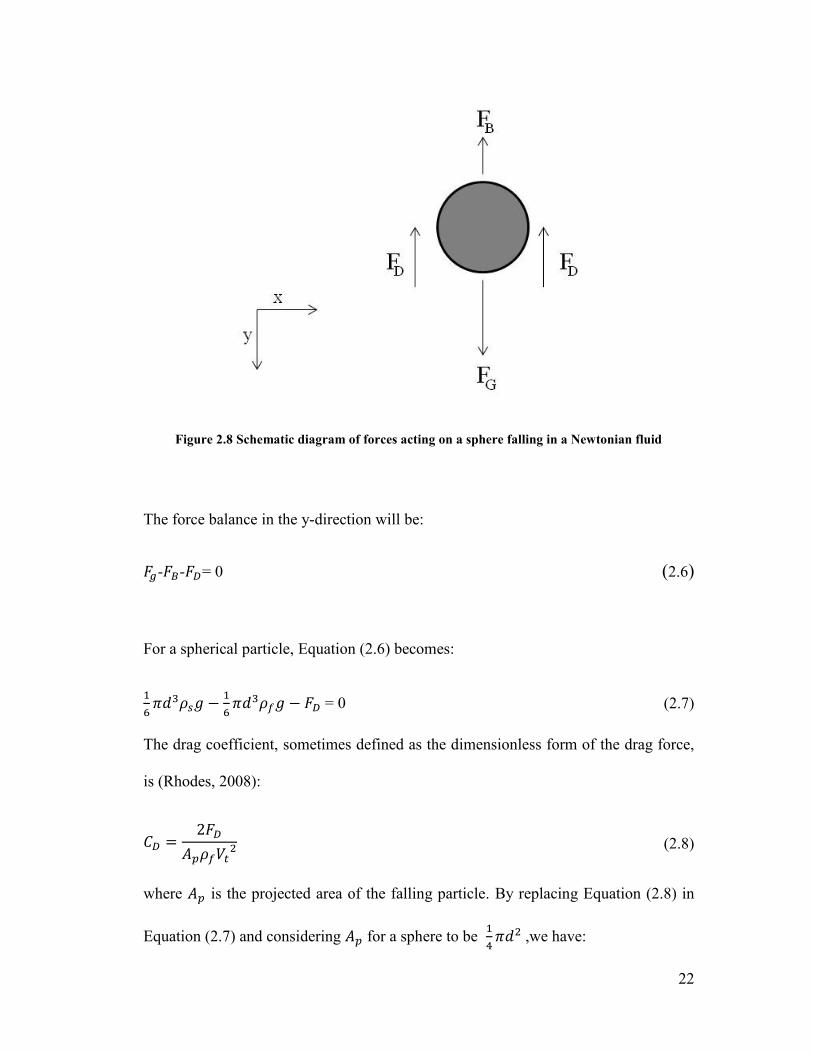
Figure 2.8 Schematic diagram of forces acting on a sphere falling in a Newtonian
fluid ............................................................................................................................. 22
Figure 2.9 Standard drag curve for a sphere falling in a Newtonian fluid (Clift et al.
1978) ........................................................................................................................... 24
Figure 2.10 Standard curve for a sphere falling in a Newtonian fluid based on the
Wilson et al. (2003) method (reproduced) .................................................................. 26
Figure 2.11 Shape of the sheared envelope surrounding a sphere in creeping motion in
viscoplastic fluid: (a) Ansley and Smith (1967); (b) Yoshioka et al. (1971); (c) Beris
et al. (1985), from Chhabra (2007) ............................................................................. 28
Figure 2.12 Yielded (white) and unyielded (black) regions for flow of a Bingham
fluid around a fixed sphere contained in a square cylinder with L/d=4 (Prashant &
Derksen, 2011) ............................................................................................................ 29
Figure 2.13 Drag curve presented by Ansley and Smith (1967) for a sphere falling in
a Bingham fluid (from Saha et al. (1992)) .................................................................. 32
vii
Figure 2.14 Overall performance of the correlation proposed by Atapattu et al. (1995)
, from Atapattu et al. (1995) ........................................................................................ 33
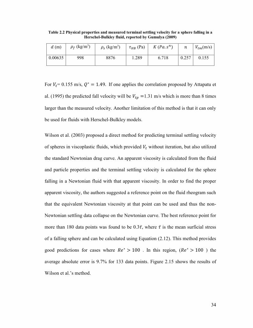
Figure 2.15 Experimental fall velocity measurements reported by Wilson et al. (2003,
2004) and shown on their standard Newtonian curve, with τref =0.3𝜏 ........................ 35
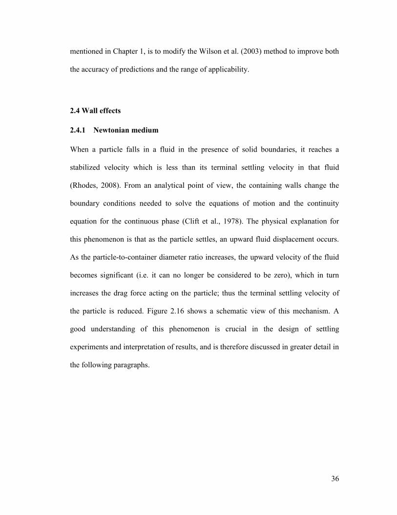
Figure 2.16 Schematic view of hindering effect of container boundaries on settling
velocity of a single sphere in a Newtonian fluid ......................................................... 37
Figure 2.17 Schematic representation of the system of a sphere falling in a tube filled
with a viscoplastic medium. Both the outer shaded regions and dark interior regions
are unyielded (Beaulne and Mitsoulis, 1997) ............................................................. 40
Figure 2.18 Size of the sheared zone around a particle moving at different velocities
in a viscoplastic fluid (λ=1/3), from Beaulne and Mitsoulis (1997) ........................... 41
Figure 3.1 Schematic view of the settling apparatus .................................................. 47
Figure 3.2 Side view (left) and top view (right) of EIT sensor electrode arrangements
..................................................................................................................................... 48
Figure 3.3 EIT reconstruction grids ............................................................................ 49
Figure 3.4 Typical conductivity measurements for two planes as an aluminum sphere
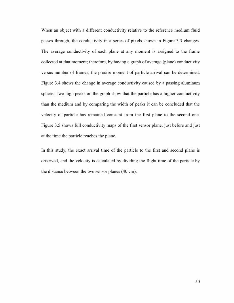
passes through each plane; Data acquisition speed was 670 fps. ............................... 51
Figure 3.5 Reconstructed conductivity maps of aluminum sphere at the moment of
arrival at the first plane (upper)................................................................................... 51
Figure 3.6 Schematic illustration of the releasing mechanism ................................... 53
Figure 4.1 Sample conductivity maps for settling tests showing straight particle
trajectory (left) and angled particle path (right) .......................................................... 64
Figure 4.2 Sample of plane averaged conductivity measurements for settling tests
with (a) a 12.7 mm aluminum sphere that has reached its terminal settling velocity
and (b) an accelerating 12.7mm steel sphere .............................................................. 65
Figure 4.3 Terminal settling velocities corrected for wall effects; tests conducted with
Newtonian fluids ......................................................................................................... 69
Figure 4.4 Time-dependent behavior for a Kaolinite-water suspension (CV=22%);
cone-and-plate rheometer; 𝜔=20 rad/s ........................................................................ 71
Figure 4.5 Settling velocity measurements for four identical 12.7 mm ceramic spheres
released at different time intervals; 15.6% Kaolinite-water mixture ......................... 72
viii
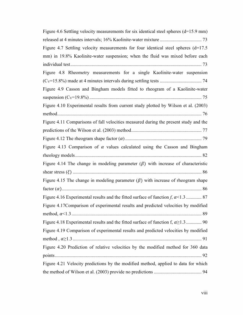
Figure 4.6 Settling velocity measurements for six identical steel spheres (d=15.9 mm)
released at 4 minutes intervals; 16% Kaolinite-water mixture ................................... 73
Figure 4.7 Settling velocity measurements for four identical steel spheres (d=17.5
mm) in 19.8% Kaolinite-water suspension; when the fluid was mixed before each
individual test .............................................................................................................. 73
Figure 4.8 Rheometry measurements for a single Kaolinite-water suspension
(CV=15.8%) made at 4 minutes intervals during settling tests ................................... 74
Figure 4.9 Casson and Bingham models fitted to rheogram of a Kaolinite-water
suspension (CV=19.8%) .............................................................................................. 75
Figure 4.10 Experimental results from current study plotted by Wilson et al. (2003)
method ......................................................................................................................... 76
Figure 4.11 Comparisons of fall velocities measured during the present study and the
predictions of the Wilson et al. (2003) method ........................................................... 77
Figure 4.12 The rheogram shape factor (𝛼) ................................................................ 79
Figure 4.13 Comparison of 𝛼 values calculated using the Casson and Bingham
rheology models .......................................................................................................... 82
Figure 4.14 The change in modeling parameter (𝛽) with increase of characteristic
shear stress (𝜉) ............................................................................................................ 86
Figure 4.15 The change in modeling parameter (𝛽) with increase of rheogram shape
factor (𝛼) ..................................................................................................................... 86
Figure 4.16 Experimental results and the fitted surface of function f, 𝛼<1.3 ............. 87
Figure 4.17Comparison of experimental results and predicted velocities by modified
method, 𝛼<1.3 ............................................................................................................. 89
Figure 4.18 Experimental results and the fitted surface of function f, 𝛼≥1.3 ............. 90
Figure 4.19 Comparison of experimental results and predicted velocities by modified
method , 𝛼≥1.3 ............................................................................................................ 91
Figure 4.20 Prediction of relative velocities by the modified method for 360 data
points ........................................................................................................................... 92
Figure 4.21 Velocity predictions by the modified method, applied to data for which
the method of Wilson et al. (2003) provide no predictions ........................................ 94
ix
Figure 4.22 Terminal settling velocity predictions using the modified method for a
sphere falling in a viscoplastic fluid ........................................................................... 95
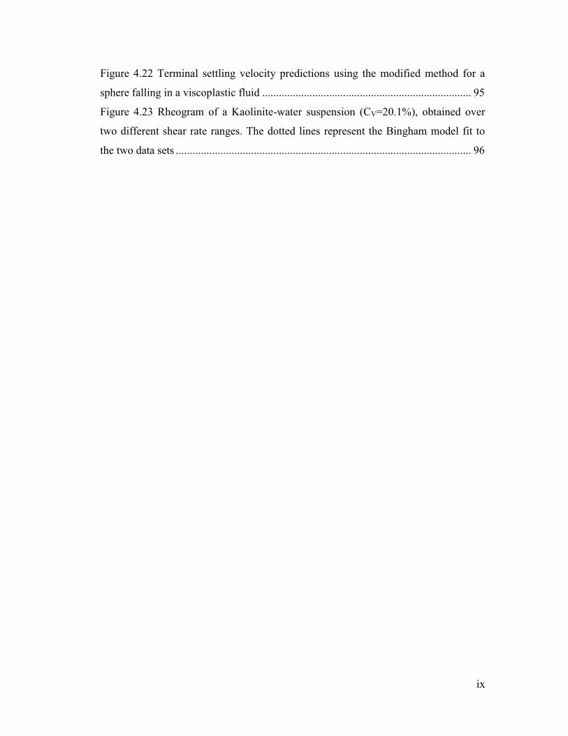
Figure 4.23 Rheogram of a Kaolinite-water suspension (CV=20.1%), obtained over
two different shear rate ranges. The dotted lines represent the Bingham model fit to
the two data sets .......................................................................................................... 96
x
List of Tables
Table 1.1 Laminar-to-turbulent transition velocities for suspensions in a 300 mm pipe
(Pullum et al. 2004) ....................................................................................................... 4
Table 2.1 Constitutive rheological models commonly used to describe viscoplastic
fluids ........................................................................................................................... 12
Table 2.2 Physical properties and measured terminal settling velocity for a sphere
falling in a Herschel-Bulkley fluid, reported by Gumulya (2009) .............................. 34
Table 2.3 Correlations for estimating wall effects for a particle settling in a
Newtonian fluid (Chhabra et al., 2003)....................................................................... 39
Table 3.1 Properties of the precision spheres used in the present study ..................... 44
Table 4.1 Measured fall velocities for single spheres in corn syrup-water solution
(CV=26%) .................................................................................................................... 67
Table 4.2 Measured fall velocities for single spheres in water ................................... 68
Table 4.3 Comparison of the performance of the modified method and Wilson et al.
(2003) method for a sphere settling in a viscoplastic fluid, 𝛼<1.3 ............................. 88
Table 4.4 Comparison of the performance of the modified method and Wilson et al.'s
method for a sphere settling in a viscoplastic fluid, 𝛼≥1.3 ......................................... 91
Table 4.5 The performance of the modified method for predicting the terminal settling
velocities of a sphere falling in a viscoplastic fluid based on choice of Bingham or
Casson fluid model ..................................................................................................... 95
Table 4.6 Velocity predictions for a steel sphere (𝜌𝑠=7684 kg/m3, d=0.01428 m) in a
Kaolinite-water suspension (CV= 20.1%, 𝜌𝑓=1331 kg/m3) fitted with two different
Bingham models based on rheology measurements made over two different shear rate
ranges .......................................................................................................................... 97
xi
List of symbols
Symbol Description Unit
Ap projected surface area of falling particle m2
𝐵𝑛 Bingham number -
𝐵𝑛∗ modeling parameter -
CD drag coefficient -
CV volume fraction -
D container diameter m
d sphere diameter m
fw wall factor -
FB buoyancy force N
FD drag force N
FG gravity force N
g gravitational acceleration m/s2
K Consistency index (Pa.s) n
L bob length m
n Power law index -
P pressure Pa
Q Dynamic parameter -
Q* modified dynamic parameter -
r radial coordinate m
R1 bob radius m
R2 cup radius m
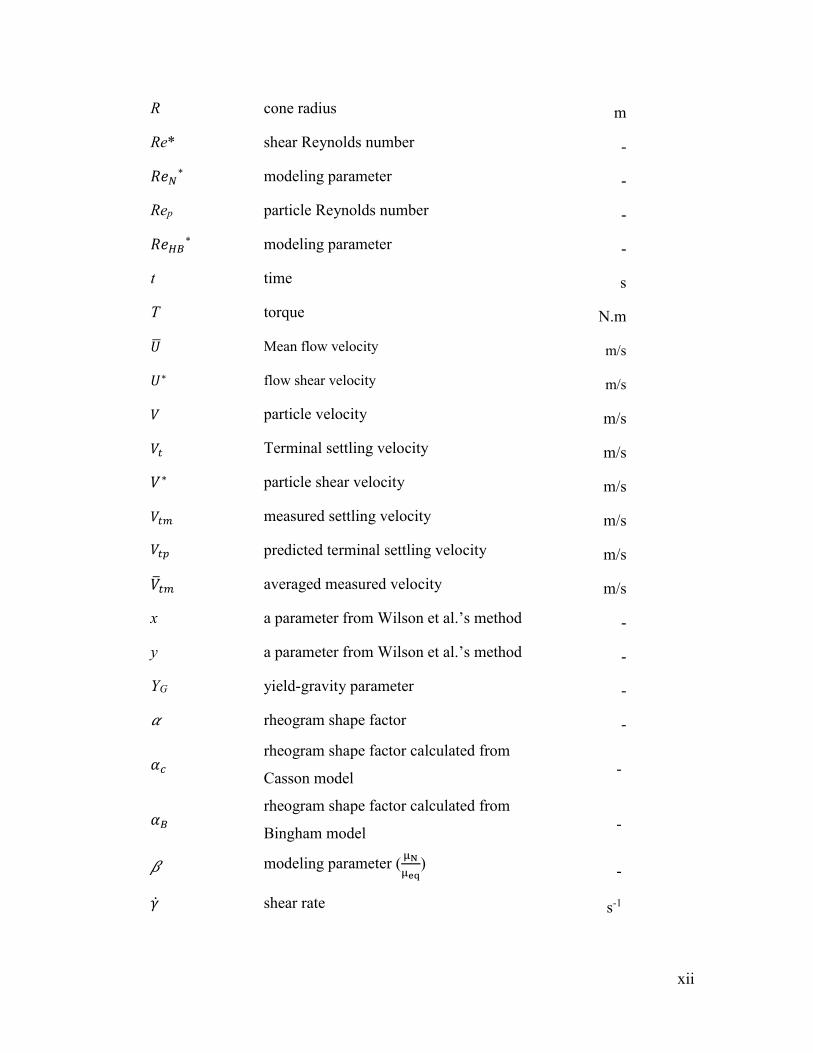
xii
R cone radius m
Re* shear Reynolds number -
𝑅𝑒𝑁∗ modeling parameter -
Rep particle Reynolds number -
𝑅𝑒𝐻𝐵∗ modeling parameter -
t time s
T torque N.m
�� Mean flow velocity m/s
𝑈∗ flow shear velocity m/s
𝑉 particle velocity m/s
𝑉𝑡 Terminal settling velocity m/s
𝑉∗ particle shear velocity m/s
𝑉𝑡𝑚 measured settling velocity m/s
𝑉𝑡𝑝 predicted terminal settling velocity m/s
��𝑡𝑚 averaged measured velocity m/s
x a parameter from Wilson et al.’s method -
y a parameter from Wilson et al.’s method -
YG yield-gravity parameter -
𝛼 rheogram shape factor -
𝛼𝑐 rheogram shape factor calculated from
Casson model -
𝛼𝐵 rheogram shape factor calculated from
Bingham model -
𝛽 modeling parameter (μN
μeq)
-
�� shear rate s-1
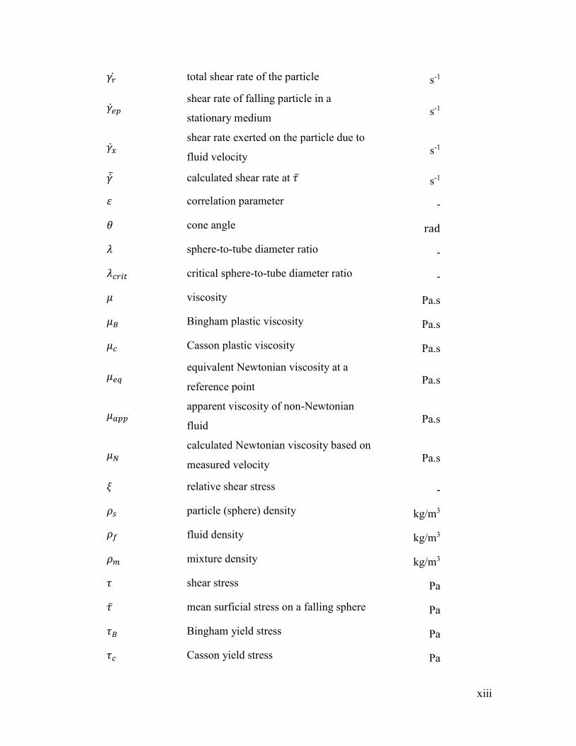
xiii
𝛾𝑟 total shear rate of the particle s-1
��𝑒𝑝 shear rate of falling particle in a
stationary medium s-1
��𝑥 shear rate exerted on the particle due to
fluid velocity s-1
�� calculated shear rate at 𝜏 s-1
𝜀 correlation parameter -
𝜃 cone angle rad
𝜆 sphere-to-tube diameter ratio -
𝜆𝑐𝑟𝑖𝑡 critical sphere-to-tube diameter ratio -
𝜇 viscosity Pa.s
𝜇𝐵 Bingham plastic viscosity Pa.s
𝜇𝑐 Casson plastic viscosity Pa.s
𝜇𝑒𝑞 equivalent Newtonian viscosity at a
reference point Pa.s
𝜇𝑎𝑝𝑝 apparent viscosity of non-Newtonian
fluid Pa.s
𝜇𝑁 calculated Newtonian viscosity based on
measured velocity Pa.s
𝜉 relative shear stress -
𝜌𝑠 particle (sphere) density kg/m3
𝜌𝑓 fluid density kg/m3
𝜌𝑚 mixture density kg/m3
𝜏 shear stress Pa
𝜏 mean surficial stress on a falling sphere Pa
𝜏𝐵 Bingham yield stress Pa
𝜏𝑐 Casson yield stress Pa
xiv
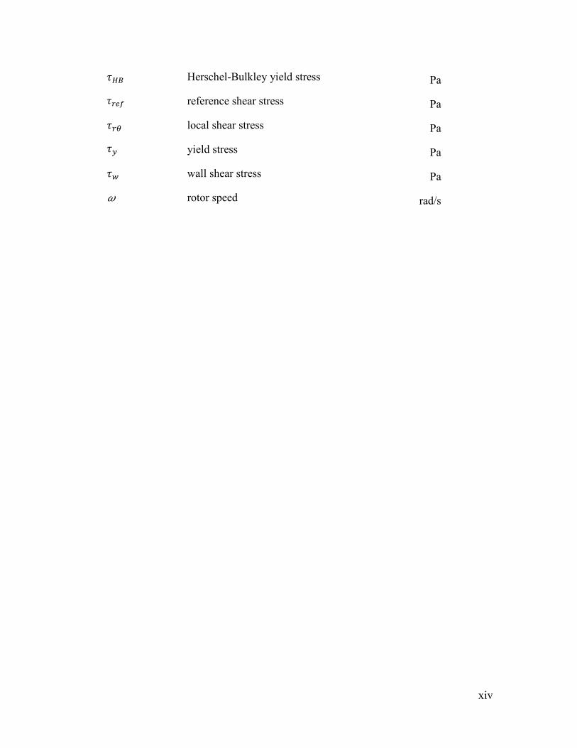
𝜏𝐻𝐵 Herschel-Bulkley yield stress Pa
𝜏𝑟𝑒𝑓 reference shear stress Pa
𝜏𝑟𝜃 local shear stress Pa
𝜏𝑦 yield stress Pa
𝜏𝑤 wall shear stress Pa
𝜔 rotor speed rad/s
1
1. Problem statement
1.1 Introduction
In the past two decades, economic and environmental considerations have had an
increasing influence on the design and operation of waste management systems in the
mining industry (Wilson et al., 2005). There has been growing pressure from
regulatory agencies to decrease water usage, and at the same time, stakeholders
demand higher rates of production to be able to compete in the growing market
(Thomas et al. 2004). As a result, producing tailings waste with higher solids
concentration has become more attractive and more necessary.
In the mine tailings disposal process, slurry pipelines are economically efficient, and
thus have become the standard mode of transportation of waste tailings (Shook et al.,
2002). The tailings stream consists of coarse particles, fine particles and a liquid
phase. In most occasions the concentration of surface-active fine particles is high
enough to form a colloidal suspension. The suspension formed from mixing the fine
particles with the liquid (often < 44 m particles + water) is referred to as the “carrier
fluid”. This type of carrier fluid invariably exhibits non-Newtonian behavior at higher
solids concentration (Shook et al. 2002; Pullum et al. 2004).
Accurate prediction of the coarse particle settling process in a non-Newtonian carrier
fluid under pipeline conditions is critical in the design, control, and operation of
pipelines, pumps, and other elements of the transportation system; for example, the
prediction of solids concentration distributions in slurry pipelines (Gillies and Shook
1994; Wilson et al. 2005; Kaushal and Tomita 2013). For spherical particles in
2
Newtonian fluids, these predictions are easily and accurately made (Whyte 1999).
The options for predicting terminal particle settling velocity in non-Newtonian fluids
are much more limited; therefore, the focus of the present study is on the prediction of
the terminal settling velocity of a spherical particle in a non-Newtonian fluid.
To explain the problem more explicitly, a typical tailings disposal system is
considered. The highly concentrated waste material from the mining complex is
transported as slurry via pipeline to the tailings area for permanent storage. This
slurry contains coarse particles, fine particles and a liquid phase (usually water). Fine
particles and water form a non-Newtonian mixture that commonly behaves as a
viscoplastic fluid (Gillies et al., 1997). This behavior is unique in that below a critical
or minimum amount of applied force, no shear rate is produced; above a critical force,
the fluid starts to flow (Chhabra, 2007). This critical minimum applied force,
normalized using the area over which the force is applied, is referred to as “yield
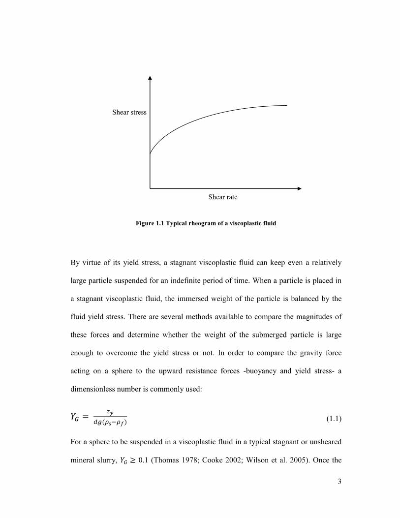
stress”. A typical example of this fluid flow behavior can be seen in Figure 1.1, which
shows the rate of deformation of a paste-like material as a function of the applied
shear stress.
3
Figure 1.1 Typical rheogram of a viscoplastic fluid
By virtue of its yield stress, a stagnant viscoplastic fluid can keep even a relatively
large particle suspended for an indefinite period of time. When a particle is placed in
a stagnant viscoplastic fluid, the immersed weight of the particle is balanced by the
fluid yield stress. There are several methods available to compare the magnitudes of
these forces and determine whether the weight of the submerged particle is large
enough to overcome the yield stress or not. In order to compare the gravity force
acting on a sphere to the upward resistance forces -buoyancy and yield stress- a
dimensionless number is commonly used:
𝑌𝐺 = 𝜏𝑦
𝑑𝑔(𝜌𝑠−𝜌𝑓) (1.1)
For a sphere to be suspended in a viscoplastic fluid in a typical stagnant or unsheared
mineral slurry, 𝑌𝐺 ≥ 0.1 (Thomas 1978; Cooke 2002; Wilson et al. 2005). Once the
Shear rate
Shear stress
4
slurry is sheared, however, even particles that were held motionless in the fluid will
begin to settle (Cooke, 2002; Chhabra, 2007). Generally, fluid turbulence is relied
upon to suspend the solids under sheared (flowing) conditions (Shook et al. 2002).
Even though it is ideal to have turbulent flow in slurry pipelines to decrease the
probability of settling, laminar flow of heterogeneous non-Newtonian slurries is
specifically attractive because, when the mixture yield stress increases, it is
economically infeasible to operate in turbulent flow (Wilson et al. 2005). The
viscoplastic nature of the carrier fluid radically delays the onset of turbulence and
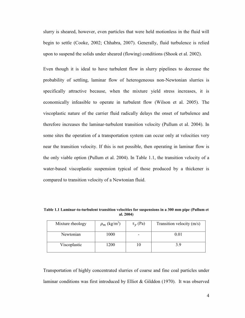
therefore increases the laminar-turbulent transition velocity (Pullum et al. 2004). In
some sites the operation of a transportation system can occur only at velocities very
near the transition velocity. If this is not possible, then operating in laminar flow is
the only viable option (Pullum et al. 2004). In Table 1.1, the transition velocity of a
water-based viscoplastic suspension typical of those produced by a thickener is
compared to transition velocity of a Newtonian fluid.
Table 1.1 Laminar-to-turbulent transition velocities for suspensions in a 300 mm pipe (Pullum et
al. 2004)
Mixture rheology 𝜌𝑚 (kg/m3) 𝜏𝑦 (Pa) Transition velocity (m/s)
Newtonian 1000 - 0.01
Viscoplastic 1200 10 3.9
Transportation of highly concentrated slurries of coarse and fine coal particles under
laminar conditions was first introduced by Elliot & Gilddon (1970). It was observed
5
that the non-Newtonian carrier fluid kept the coarse particles suspended at the center
of the pipe and this phenomenon essentially reduced the total pressure gradient in the
test pipe loop. This type of laminar flow was referred to as “stabilized flow”. Later,
visualization studies showed that when the fluid is being sheared, the particles which
were held suspended in an unsheared (stagnant) fluid tend to settle given enough time
(Graham et al, 2003; Pullum 2003). Experiments done by Thomas et al. (2004)
confirmed those observations and showed that the settling occurs quickly during the
shearing that occurs in a pipeline. After a short amount of time, these settled particles
were observed to form a sliding bed which moved more slowly than the rest of the
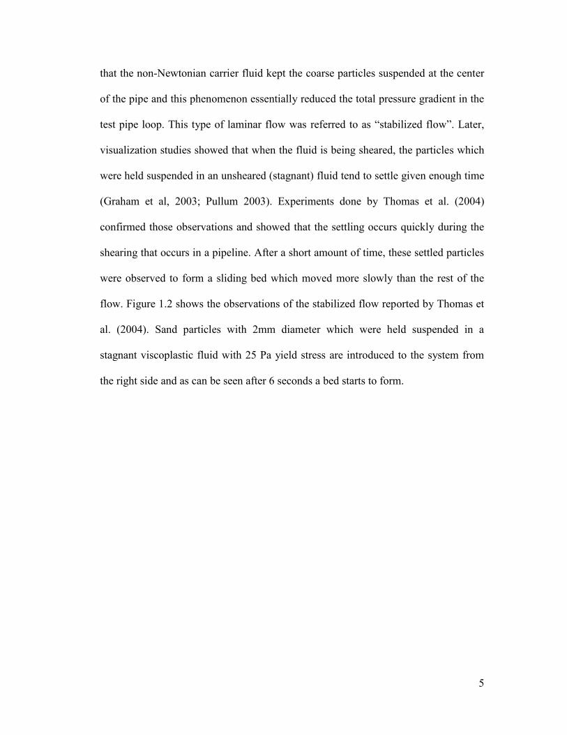
flow. Figure 1.2 shows the observations of the stabilized flow reported by Thomas et
al. (2004). Sand particles with 2mm diameter which were held suspended in a
stagnant viscoplastic fluid with 25 Pa yield stress are introduced to the system from
the right side and as can be seen after 6 seconds a bed starts to form.
6
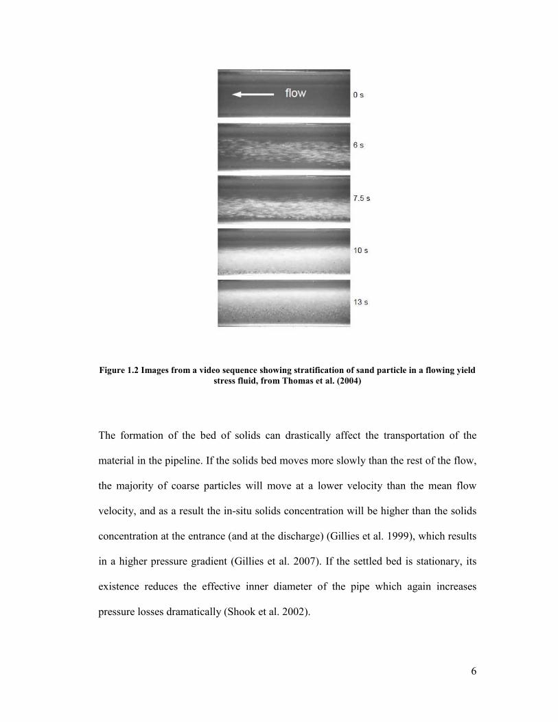
Figure 1.2 Images from a video sequence showing stratification of sand particle in a flowing yield
stress fluid, from Thomas et al. (2004)
The formation of the bed of solids can drastically affect the transportation of the
material in the pipeline. If the solids bed moves more slowly than the rest of the flow,
the majority of coarse particles will move at a lower velocity than the mean flow
velocity, and as a result the in-situ solids concentration will be higher than the solids
concentration at the entrance (and at the discharge) (Gillies et al. 1999), which results
in a higher pressure gradient (Gillies et al. 2007). If the settled bed is stationary, its
existence reduces the effective inner diameter of the pipe which again increases
pressure losses dramatically (Shook et al. 2002).
7
These observations suggest that the mechanism of particle settling in viscoplastic
fluids is completely different in a stagnant fluid than in a sheared medium. To model
complexities of settling process in flowing viscoplastic fluid, Wilson et al. (2004)
introduced an equation for total shear rate applied to a coarse particle in a sheared
carrier fluid:
��𝑟 = [ (��𝑒𝑝)2 + (��𝑥)2 ]0.5 (1.2)
where ��𝑒𝑝 is the shear rate of the falling particle in a stationary medium, ��𝑥 is the
additional shear rate exerted on the particle due to fluid velocity and ��𝑟 is the resultant
total shear rate. As Equation (1.2) shows, a particle is exposed to a higher shear rate
in a sheared medium than in a stationary fluid. For a typical rheological behavior of a
viscoplastic fluid, such as the rheogram shown in Figure 1.1, a high shear rate
corresponds to a lower viscosity. With a small viscosity, the particle falls more
rapidly. Equation (1.2) suggests that a suspended particle in a sheared fluid settles and
the fall velocity is higher than the fall velocity in a stagnant fluid. This prediction is in
agreement with several observations in the literature (Graham et al. 2003; Thomas et
al. 2004; Pullum et al. 2004; Gillies et al. 2007, Talmon et al. 2014).
Accurate prediction of ��𝑒𝑝 and ��𝑥 is therefore essential in predicting the settling
behavior of particles transported by pipeline. For that reason, prediction of the
terminal settling velocity of a particle in a stagnant viscoplastic fluid is an important
area of research.
There are several available methods to predict the terminal settling velocity of a
spherical particle in a Newtonian fluid; for a particle settling in a viscoplastic fluid,
8
however, there are a limited number of techniques available in the literature.
Analytical methods have led to limited results for highly constrained, carefully
specified systems (Chhabra 2007). Several correlations have been developed to offer
a convenient solution to the problem for engineering purposes. These different
approaches will be reviewed in Chapter 2.
One of the practical problems in predicting terminal settling velocity – even in
Newtonian fluids – is that usually an iterative procedure is required. Wilson et al.
(2003) introduced a new method to predict the terminal settling velocity of spheres in
Newtonian fluids directly, but the more important aspect of the proposed method was
that it was also able to predict the terminal settling velocity of a sphere in a non-
Newtonian, viscoplastic fluid by using an “apparent viscosity”. Apparent viscosity is
a single number that is calculated based on the physical properties of the system and
is able to represent the rheology of the fluid in that specific fluid-particle system. This
method not only provides direct predictions for terminal settling velocities of spheres
in viscoplastic fluids, it is also applicable to a wide range of system properties.
There are features of this method that limit both its applicability and its prediction
accuracy. These shortcomings − which will be discussed in detail in Chapter 2− can
dramatically limit the prediction of the fluid-particle settling conditions. Also
industrially important conditions cannot always be modeled using this method. For
this reason, a modified direct prediction method is required to predict the settling
occurrence, and to provide a reasonably accurate estimation of the terminal settling
velocity for a wide range of system properties.
9
1.2 Project objectives
The primary objective of this research is to develop a method to accurately predict
terminal settling velocity of a sphere in a viscoplastic fluid. In order to do this, an
experimental approach has been taken. The major activities that must be completed to
meet this objective are:
To analyze and evaluate existing methods of prediction for terminal settling
velocity of spheres in viscoplastic fluids and identify the strength and
limitations of each method;
To develop a system of experimental equipment and a methodology through
which the terminal settling velocity of a sphere in a viscoplastic suspension
can be accurately measured for a wide range of fluid-particle system
properties;
To develop an inclusive and accurate direct method for predicting the terminal
settling velocity of a sphere in a viscoplastic fluid based on the experimental
results obtained from the present investigation and from experimental results
available in literature.
10
2. Background
2.1 Rheology of viscoplastic fluids
2.1.1 Rheology models
When a Newtonian fluid is subjected to an applied force, the rate of deformation has a
linear relationship with that force (Bird et al. 2007). Under laminar viscous flow
conditions, the slope of this line, i.e. the Newtonian viscosity, is constant and
independent of the force applied, the shear rate range, or time. Any deviation from
this behavior is described as non-Newtonian behavior. There are several models to
represent non-Newtonian fluid behavior; in some cases, more than one model can
represent the fluid rheological properties. The focus here is on time-independent non-
Newtonian behavior.
Among non-Newtonian fluids, the “viscoplastic” category is used to describe fluids
that exhibit a yield stress. Although the existence of “true yield stress” in viscoplastic
materials has been a subject of debate (Barnes and Walters, 1985), the concept has
proven to be extremely useful in practice. The physical meaning of yield stress is
often related to the postulation that the fluid at rest has a structure that will not break
unless the external stress exceeds a minimum value (Andres 1961; Hariharaputhiran
et al. 1998).
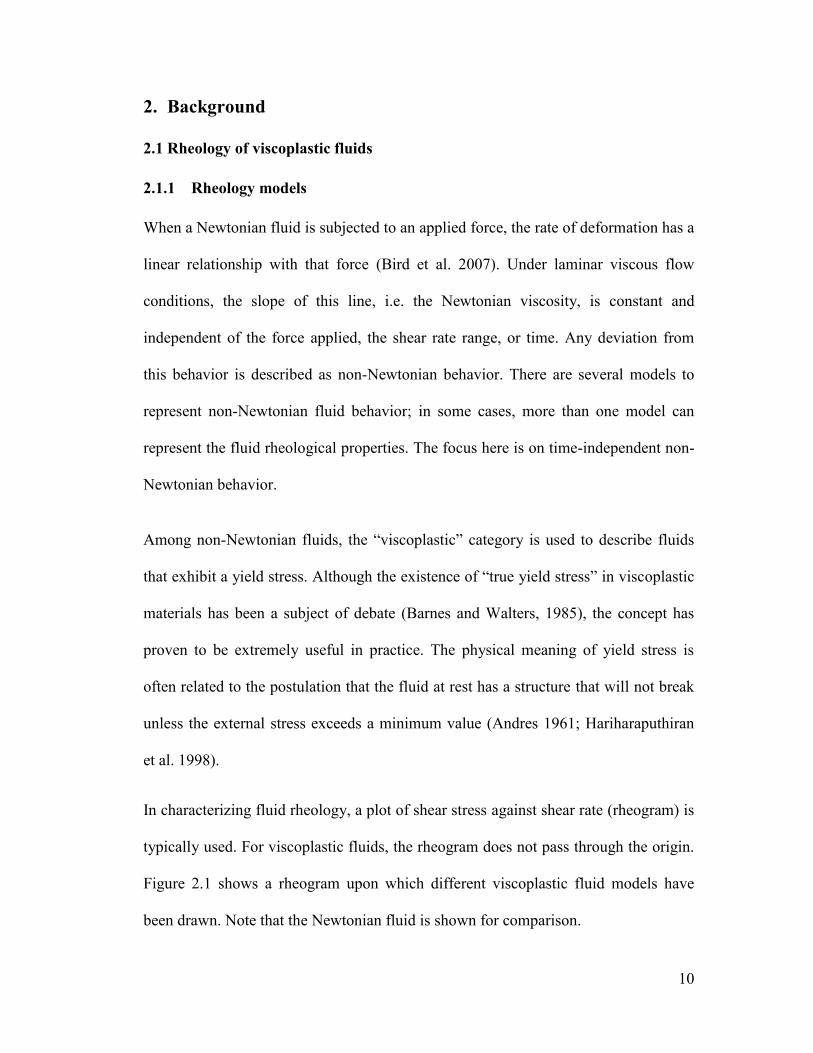
In characterizing fluid rheology, a plot of shear stress against shear rate (rheogram) is
typically used. For viscoplastic fluids, the rheogram does not pass through the origin.
Figure 2.1 shows a rheogram upon which different viscoplastic fluid models have
been drawn. Note that the Newtonian fluid is shown for comparison.
11
Figure 2.1 Typical rheograms for viscoplastic fluids
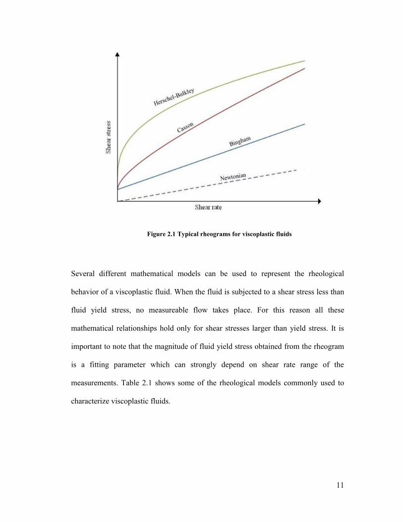
Several different mathematical models can be used to represent the rheological
behavior of a viscoplastic fluid. When the fluid is subjected to a shear stress less than
fluid yield stress, no measureable flow takes place. For this reason all these
mathematical relationships hold only for shear stresses larger than yield stress. It is
important to note that the magnitude of fluid yield stress obtained from the rheogram
is a fitting parameter which can strongly depend on shear rate range of the
measurements. Table 2.1 shows some of the rheological models commonly used to
characterize viscoplastic fluids.
12
Table 2.1 Constitutive rheological models commonly used to describe
viscoplastic fluids
Newtonian* 𝜏 = 𝜇��
Bingham 𝜏 = 𝜇𝐵�� + 𝜏𝐵
Casson 𝜏0.5 = 𝜇𝑐0.5��0.5 + 𝜏𝑐
0.5
Herschel-Bulkley 𝜏 = 𝐾��𝑛 + 𝜏𝐻𝐵
* Provided for comparison; not used for viscoplastic fluids
2.1.2 Rheometry
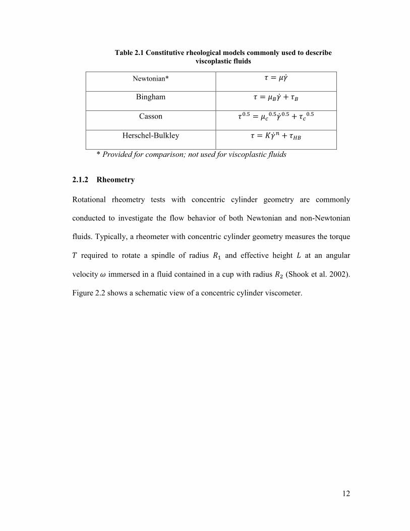
Rotational rheometry tests with concentric cylinder geometry are commonly
conducted to investigate the flow behavior of both Newtonian and non-Newtonian
fluids. Typically, a rheometer with concentric cylinder geometry measures the torque
𝑇 required to rotate a spindle of radius 𝑅1 and effective height 𝐿 at an angular
velocity 𝜔 immersed in a fluid contained in a cup with radius 𝑅2 (Shook et al. 2002).
Figure 2.2 shows a schematic view of a concentric cylinder viscometer.
13
Figure 2.2 Schematic view of concentric cylinder apparatus
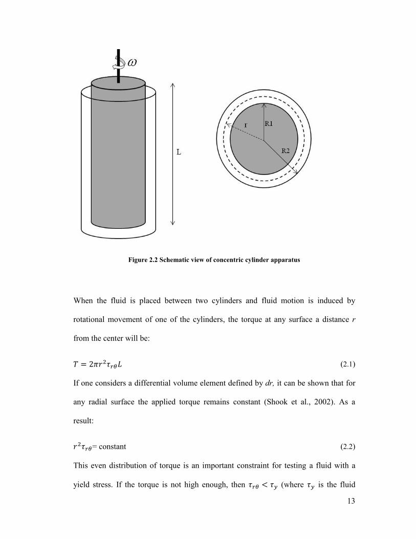
When the fluid is placed between two cylinders and fluid motion is induced by
rotational movement of one of the cylinders, the torque at any surface a distance r
from the center will be:
𝑇 = 2𝜋𝑟2𝜏𝑟𝜃𝐿 (2.1)
If one considers a differential volume element defined by dr, it can be shown that for
any radial surface the applied torque remains constant (Shook et al., 2002). As a
result:
𝑟2𝜏𝑟𝜃= constant (2.2)
This even distribution of torque is an important constraint for testing a fluid with a
yield stress. If the torque is not high enough, then 𝜏𝑟𝜃 < 𝜏𝑦 (where 𝜏𝑦 is the fluid
14
yield stress), some fluid in the gap adjacent to the cup wall (𝑅2) will be unsheared.
For this reason a minimum torque must be provided to ensure the fluid in the gap is
fully sheared. This limitation does not allow for measurements in low shear rate
regions. In evaluating the problem of a sphere settling in a viscoplastic fluid, the shear
rate of the fluid surrounding the falling particle is often low. Because of the
aforementioned torque limitation, it may be that such low shear rates cannot be tested
using a concentric cylinder viscometer.
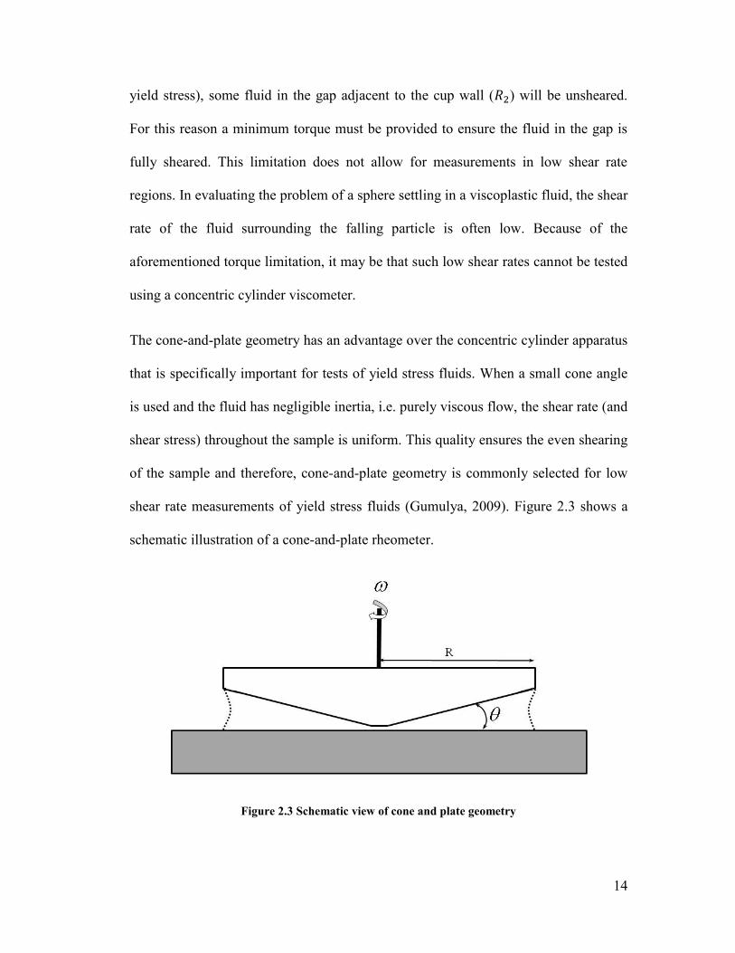
The cone-and-plate geometry has an advantage over the concentric cylinder apparatus
that is specifically important for tests of yield stress fluids. When a small cone angle
is used and the fluid has negligible inertia, i.e. purely viscous flow, the shear rate (and
shear stress) throughout the sample is uniform. This quality ensures the even shearing
of the sample and therefore, cone-and-plate geometry is commonly selected for low
shear rate measurements of yield stress fluids (Gumulya, 2009). Figure 2.3 shows a
schematic illustration of a cone-and-plate rheometer.
Figure 2.3 Schematic view of cone and plate geometry
15
For a cone-and-plate geometry, conversion of angular velocity and measured torque
to shear rate and shear stress is possible using (AR-G2 manual)
𝜏 =1
2
3𝜋𝑅3
× 𝑇 (2.3)
�� =1
𝜃× 𝜔 (2.4)
2.2 Kaolinite-water suspensions
2.2.1 Origins of viscoplastic behavior
Clay particles have a high surface-to-mass ratio, meaning that when they are placed in
water, a colloidal suspension is produced. In colloidal suspensions the particle-
particle interactions are often modeled using the DLVO theory, which is a sum of the
attractive van der Waals forces and repulsive electrostatic forces caused by charged
surfaces of the particles (Masliyah et al., 2011). The relative magnitudes of these
interactions determine the rheology of the mixture (Masliyah et al., 2011). Michaels
and Bolger (1962), in a classic work, analyzed and characterized different types of
particle-particle interactions in Kaolinite-water suspensions. They showed that if the
attractive van der Waals forces are dominant, the particles attach to each other and
form flocs. If the attractive forces are large enough, the flocs will form aggregates.
Alternatively, if repulsive electrostatic forces are dominant, particles remain dispersed
(Masliyah et al. 2011).
Kaolinite particles are plate-like units which stack face to face to form a lattice crystal
(Michaels and Bolger, 1962). When the Kaolinite particles are placed in water, the
surface of these plates bears a negative charge, but the charge on the surface and
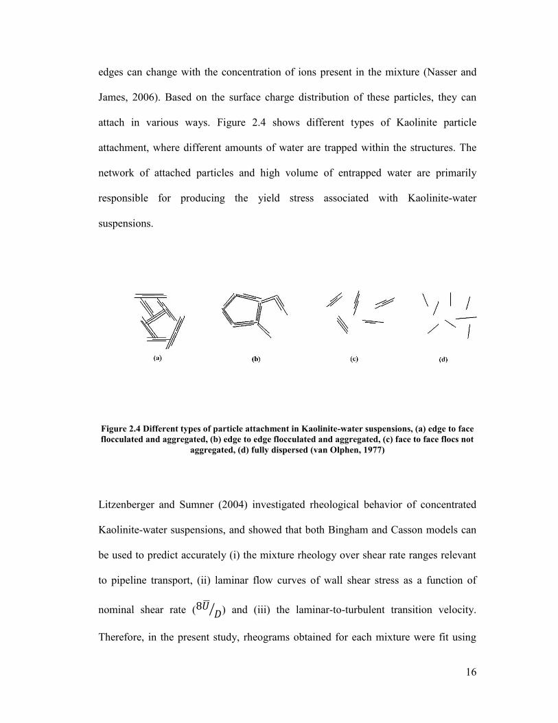
16
edges can change with the concentration of ions present in the mixture (Nasser and
James, 2006). Based on the surface charge distribution of these particles, they can
attach in various ways. Figure 2.4 shows different types of Kaolinite particle
attachment, where different amounts of water are trapped within the structures. The
network of attached particles and high volume of entrapped water are primarily
responsible for producing the yield stress associated with Kaolinite-water
suspensions.
Figure 2.4 Different types of particle attachment in Kaolinite-water suspensions, (a) edge to face
flocculated and aggregated, (b) edge to edge flocculated and aggregated, (c) face to face flocs not
aggregated, (d) fully dispersed (van Olphen, 1977)
Litzenberger and Sumner (2004) investigated rheological behavior of concentrated
Kaolinite-water suspensions, and showed that both Bingham and Casson models can
be used to predict accurately (i) the mixture rheology over shear rate ranges relevant
to pipeline transport, (ii) laminar flow curves of wall shear stress as a function of
nominal shear rate (8��𝐷⁄ ) and (iii) the laminar-to-turbulent transition velocity.
Therefore, in the present study, rheograms obtained for each mixture were fit using
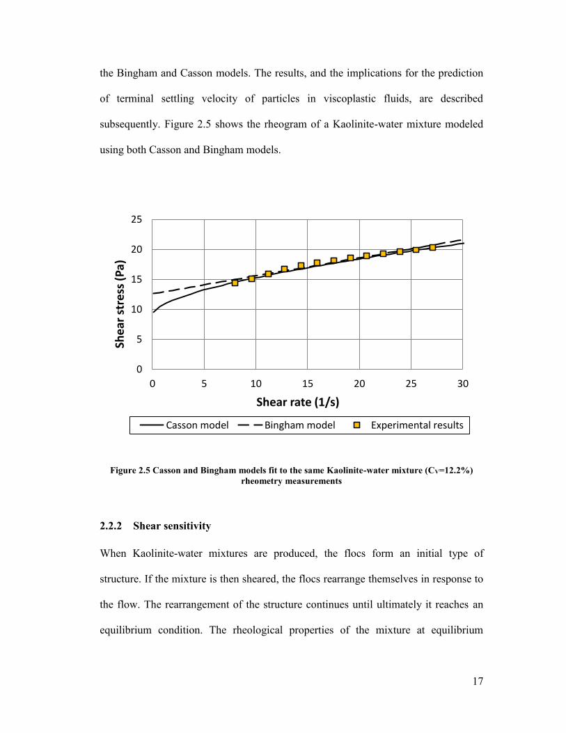
17
the Bingham and Casson models. The results, and the implications for the prediction
of terminal settling velocity of particles in viscoplastic fluids, are described
subsequently. Figure 2.5 shows the rheogram of a Kaolinite-water mixture modeled
using both Casson and Bingham models.
Figure 2.5 Casson and Bingham models fit to the same Kaolinite-water mixture (CV=12.2%)
rheometry measurements
2.2.2 Shear sensitivity
When Kaolinite-water mixtures are produced, the flocs form an initial type of
structure. If the mixture is then sheared, the flocs rearrange themselves in response to
the flow. The rearrangement of the structure continues until ultimately it reaches an
equilibrium condition. The rheological properties of the mixture at equilibrium
0
5
10
15
20
25
0 5 10 15 20 25 30
She
ar s
tre
ss (
Pa
)
Shear rate (1/s)
Casson model Bingham model Experimental results
18
depend on two parameters; the shearing rate and the exposure time to shear (Schaan
et al. 2004).
Shear sensitivity can be detected by online torque measurements taken during
shearing. Schaan et al. (2004) have shown that the minimum time required to reach an
equilibrium state is a function of shear rate in mixing process; higher shear rates can
take the mixture to equilibrium more rapidly.
After shearing ceases the links between the flocs are re-established primarily through
Brownian motion and particle collision (van Olphen, 1977). This effect causes the
yield stress to increase with time when the mixture is left at rest. Thixotropic effects
can dramatically change the properties of viscoplastic fluids once they are no longer
exposed to shear (Nguyen and Boger, 1997).
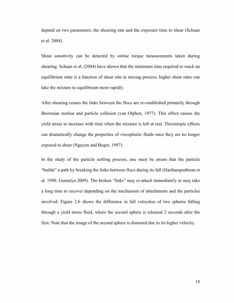
In the study of the particle settling process, one must be aware that the particle
“builds” a path by breaking the links between flocs during its fall (Hariharaputhiran et
al. 1998; Gumulya 2009). The broken “links” may re-attach immediately or may take
a long time to recover depending on the mechanism of attachments and the particles
involved. Figure 2.6 shows the difference in fall velocities of two spheres falling
through a yield stress fluid, where the second sphere is released 2 seconds after the
first. Note that the image of the second sphere is distorted due to its higher velocity.
19
Figure 2.6 Two vertically aligned identical bronze spheres (7.94 mm diameter), released with 2
seconds delay, in 1.1% Floxit solution (Gumulya, 2009)
2.2.3 Determining yield stress
The magnitude of the mixture yield stress becomes especially important when it
comes to the problem of settling particles. In order to compare the downward gravity
force of a falling sphere to the upward resistance forces -buoyancy and yield stress- a
dimensionless number is commonly used:
𝑌𝐺 = 𝜏𝑦
𝑑𝑔(𝜌𝑠−𝜌𝑓) (2.5)
The question of whether a sphere would or would not settle in an unsheared
viscoplastic medium has attracted attention in the literature. For example, Boardman
and Whitmore (1961), Ansley and Smith (1967), Beris et al. (1985) and Chafe and de
Bruyn (2005) have used Bingham fluids and reported a range between 0.048 to 0.2
20
for maximum 𝑌𝐺 as a necessary condition for the sphere to move, while others like
Uhlherr (1986) and Atapattu (1989) have used vane yield stress measurements as a
basis for their analysis and reported different values. Part of the disagreement of
results is due to different methods used by researchers to determine the yield stress of
the mixture. As was mentioned earlier, the yield stress obtained from a viscoplastic
rheology model is a fitting parameter and can vary significantly depending on the
method used. Figure 2.5 shows the difference between 𝜏𝐵 and 𝜏𝑐 for the same set of
measurements. In this example, the Bingham model gives 𝜏𝐵 =12.6 Pa while the
Casson model gives 𝜏𝐶 =8.9 Pa.
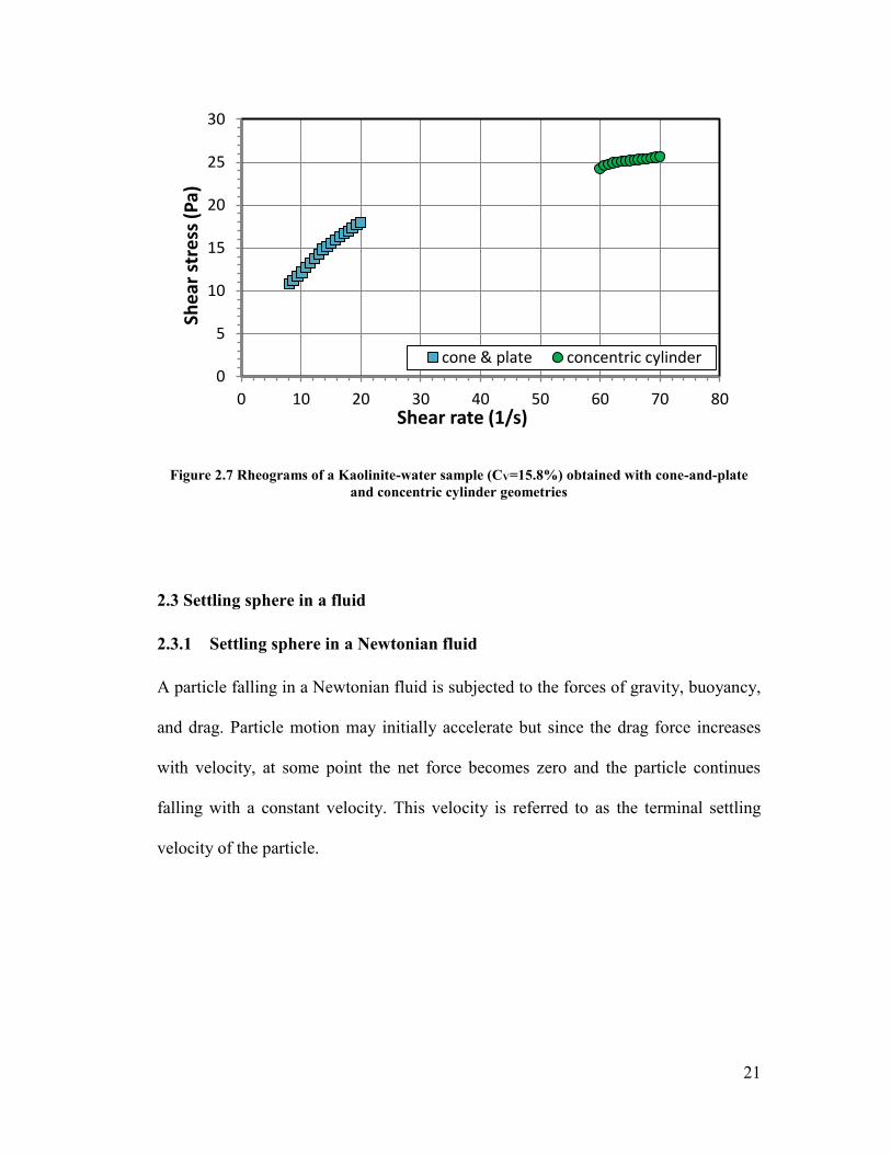
Another parameter that can affect the magnitude of the fitted yield stress is the
technique used for the rheometry tests. Measurements must be made over the relevant
shear rate range when working with viscoplastic fluids such as Kaolinite-water
mixtures. Figure 2.7 shows the rheogram of the same suspension from cone-and-plate
and concentric cylinder rheometry. The requirement to ensure 𝜏|𝑅2 ≥ 𝜏𝑦 during
concentric cylinder rheometry tests of viscoplastic fluids means that the “typical”
shear rate range for this geometry is ~ 20-200 s-1. Note how the results of the two
rheometry tests shown in Figure 2.7 produce substantially different yield stress
values; 𝜏𝑦= 6.1 Pa for the cone-and-plate measurements, and 𝜏𝑦=17.9 Pa for the
concentric cylinder viscometer.
21
Figure 2.7 Rheograms of a Kaolinite-water sample (CV=15.8%) obtained with cone-and-plate
and concentric cylinder geometries
2.3 Settling sphere in a fluid
2.3.1 Settling sphere in a Newtonian fluid
A particle falling in a Newtonian fluid is subjected to the forces of gravity, buoyancy,
and drag. Particle motion may initially accelerate but since the drag force increases
with velocity, at some point the net force becomes zero and the particle continues
falling with a constant velocity. This velocity is referred to as the terminal settling
velocity of the particle.
0
5
10
15
20
25
30
0 10 20 30 40 50 60 70 80
She
ar s
tre
ss (
Pa)
Shear rate (1/s)
cone & plate concentric cylinder
22
Figure 2.8 Schematic diagram of forces acting on a sphere falling in a Newtonian fluid
The force balance in the y-direction will be:
𝐹𝑔-𝐹𝐵-𝐹𝐷= 0 (2.6)
For a spherical particle, Equation (2.6) becomes:
1
6𝜋𝑑3𝜌𝑠𝑔 −
1
6𝜋𝑑3𝜌𝑓𝑔 − 𝐹𝐷 = 0 (2.7)
The drag coefficient, sometimes defined as the dimensionless form of the drag force,
is (Rhodes, 2008):
𝐶𝐷 =2𝐹𝐷
𝐴𝑝𝜌𝑓𝑉𝑡2 (2.8)
where 𝐴𝑝 is the projected area of the falling particle. By replacing Equation (2.8) in
Equation (2.7) and considering 𝐴𝑝 for a sphere to be 1
4𝜋𝑑2 ,we have:
23
𝐶𝐷 = 4(𝜌𝑠−𝜌𝑓)𝑑𝑔
3𝑉𝑡2𝜌𝑓
(2.9)
For low particle Reynolds numbers, 𝑅𝑒𝑝 < 0.3 (Rhodes, 2008), Stokes (1851)
showed that
𝐶𝐷 =24
𝑅𝑒𝑝 (2.10)
where the particle Reynolds number is
𝑅𝑒𝑝 =𝑑𝜌𝑓𝑉𝑡
𝜇 (2.11)
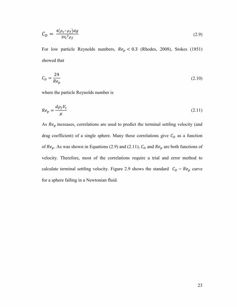
As 𝑅𝑒𝑝 increases, correlations are used to predict the terminal settling velocity (and
drag coefficient) of a single sphere. Many these correlations give 𝐶𝐷 as a function
of 𝑅𝑒𝑝. As was shown in Equations (2.9) and (2.11), 𝐶𝐷 and 𝑅𝑒𝑝 are both functions of
velocity. Therefore, most of the correlations require a trial and error method to
calculate terminal settling velocity. Figure 2.9 shows the standard 𝐶𝐷 − 𝑅𝑒𝑝 curve
for a sphere falling in a Newtonian fluid.
24
Figure 2.9 Standard drag curve for a sphere falling in a Newtonian fluid (Clift et al. 1978)
In order to provide direct predictions of terminal settling velocity of a sphere in a
Newtonian fluid, Wilson et al. (2003) adopted the pipe flow analysis of Prandtl
(1933) and Colebrook (1938) to develop a new set of equations based on shear
velocity (𝑉∗) and shear Reynolds number (𝑅𝑒∗).
In pipe flow, shear velocity ( 𝑈∗) is the square root of the ratio of the shear stress at
the pipe wall to the fluid density and shear Reynolds number (𝑅𝑒∗) is calculated
based on 𝑈∗. One major difference between the pipe-flow analysis and the flow
around a falling particle is that the stress distribution around the particle is not
uniform (Wilson et al. 2003). In order to represent the characteristic shear stress of
this process, the mean surficial stress (𝜏) of a falling particle was chosen, where
𝜏 represents the immersed weight of the particle divided by its total surface area:
𝜏 =𝑑𝑔(𝜌𝑠 − 𝜌𝑓)
6 (2.12)
25
Considering the definition of shear velocity (𝑈∗), the parameter 𝑉∗ for a settling
particle will be:
𝑉∗ = √��
𝜌𝑓= √
𝑑𝑔(𝜌𝑠−𝜌𝑓)
6𝜌𝑓 (2.13)
The shear Reynolds number can be therefore written as:
𝑅𝑒∗ =𝑑𝜌𝑓𝑉∗
𝜇 (2.14)
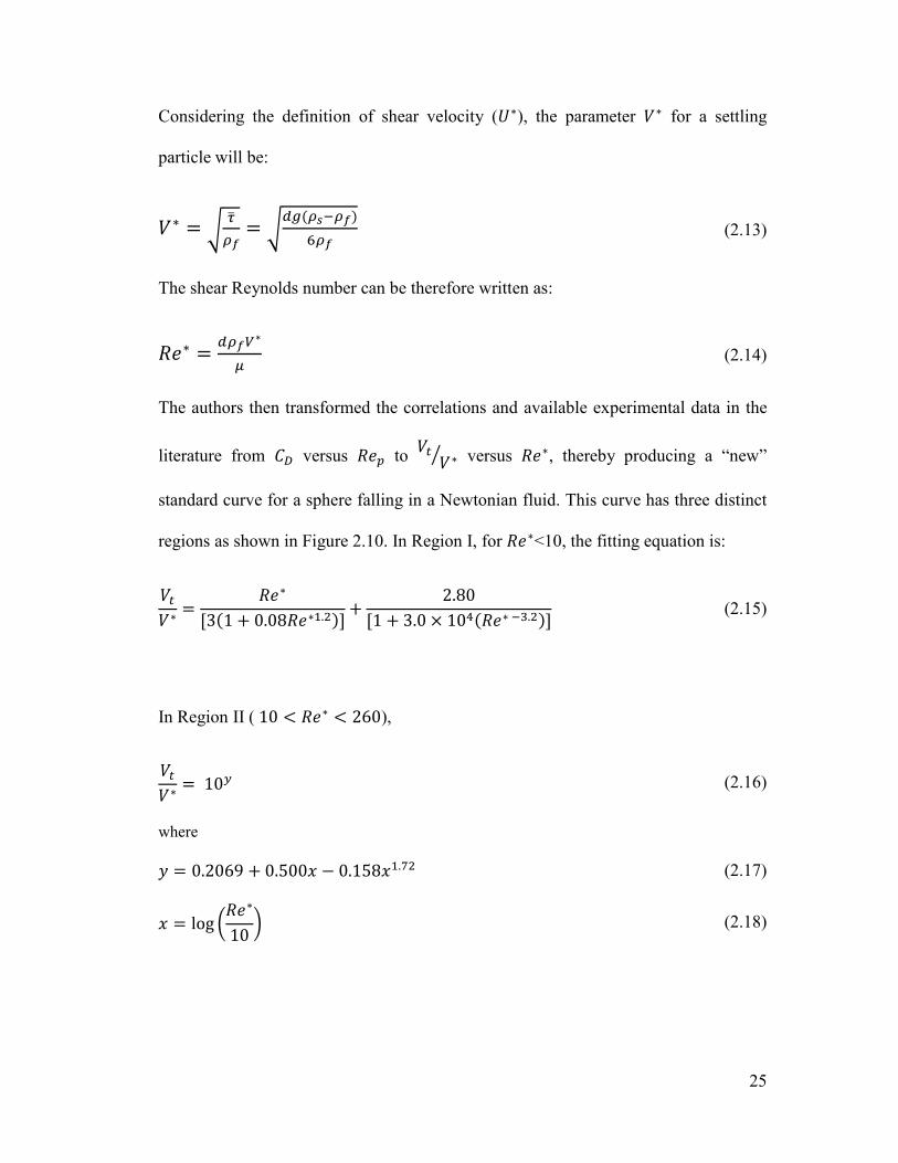
The authors then transformed the correlations and available experimental data in the
literature from 𝐶𝐷 versus 𝑅𝑒𝑝 to 𝑉𝑡
𝑉∗⁄ versus 𝑅𝑒∗, thereby producing a “new”
standard curve for a sphere falling in a Newtonian fluid. This curve has three distinct
regions as shown in Figure 2.10. In Region I, for 𝑅𝑒∗<10, the fitting equation is:
𝑉𝑡
𝑉∗=
𝑅𝑒∗
[3(1 + 0.08𝑅𝑒∗1.2)]+
2.80
[1 + 3.0 × 10⁴(𝑅𝑒∗ −3.2)] (2.15)
In Region II ( 10 < 𝑅𝑒∗ < 260),
𝑉𝑡
𝑉∗= 10𝑦 (2.16)
where
𝑦 = 0.2069 + 0.500𝑥 − 0.158𝑥1.72 (2.17)
𝑥 = log (𝑅𝑒∗
10) (2.18)
26
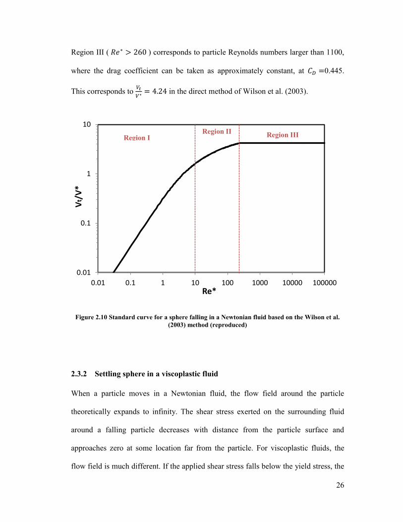
Region III ( 𝑅𝑒∗ > 260 ) corresponds to particle Reynolds numbers larger than 1100,
where the drag coefficient can be taken as approximately constant, at 𝐶𝐷 =0.445.
This corresponds to 𝑉𝑡
𝑉∗ = 4.24 in the direct method of Wilson et al. (2003).
Figure 2.10 Standard curve for a sphere falling in a Newtonian fluid based on the Wilson et al.
(2003) method (reproduced)
2.3.2 Settling sphere in a viscoplastic fluid
When a particle moves in a Newtonian fluid, the flow field around the particle
theoretically expands to infinity. The shear stress exerted on the surrounding fluid
around a falling particle decreases with distance from the particle surface and
approaches zero at some location far from the particle. For viscoplastic fluids, the
flow field is much different. If the applied shear stress falls below the yield stress, the
0.01
0.1
1
10
0.01 0.1 1 10 100 1000 10000 100000
Vt/
V*
Re*
Region IIRegion IIIRegion I
27
fluid acts as an elastic solid instead of a viscous material. For this reason, there are
different zones in the fluid surrounding a falling particle.
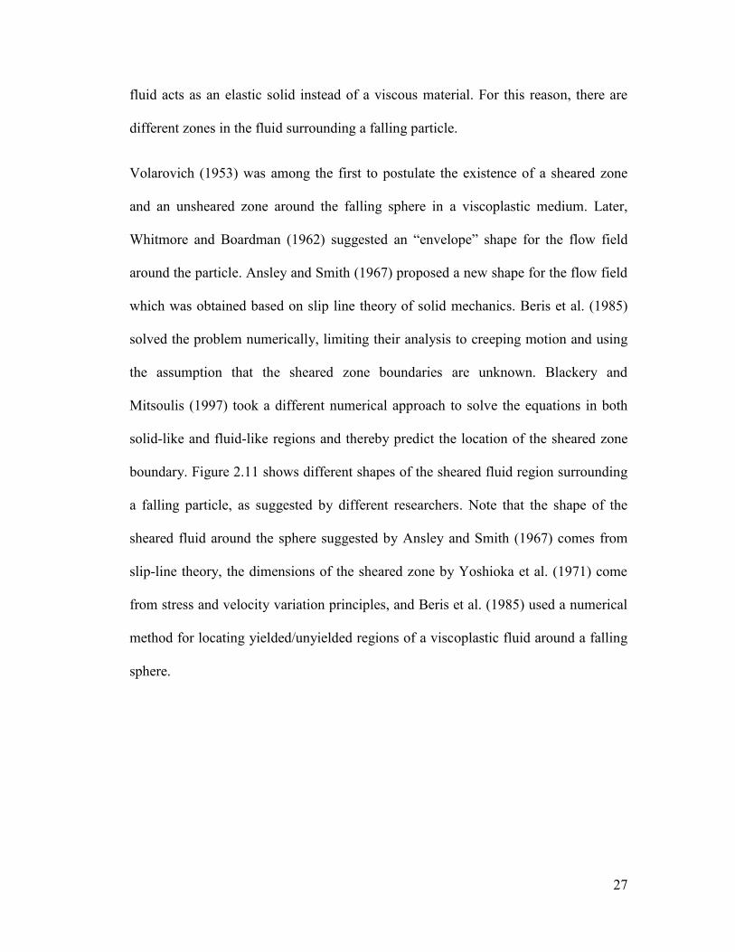
Volarovich (1953) was among the first to postulate the existence of a sheared zone
and an unsheared zone around the falling sphere in a viscoplastic medium. Later,
Whitmore and Boardman (1962) suggested an “envelope” shape for the flow field
around the particle. Ansley and Smith (1967) proposed a new shape for the flow field
which was obtained based on slip line theory of solid mechanics. Beris et al. (1985)
solved the problem numerically, limiting their analysis to creeping motion and using
the assumption that the sheared zone boundaries are unknown. Blackery and
Mitsoulis (1997) took a different numerical approach to solve the equations in both
solid-like and fluid-like regions and thereby predict the location of the sheared zone
boundary. Figure 2.11 shows different shapes of the sheared fluid region surrounding
a falling particle, as suggested by different researchers. Note that the shape of the
sheared fluid around the sphere suggested by Ansley and Smith (1967) comes from
slip-line theory, the dimensions of the sheared zone by Yoshioka et al. (1971) come
from stress and velocity variation principles, and Beris et al. (1985) used a numerical
method for locating yielded/unyielded regions of a viscoplastic fluid around a falling
sphere.
28
Figure 2.11 Shape of the sheared envelope surrounding a sphere in creeping motion in
viscoplastic fluid: (a) Ansley and Smith (1967); (b) Yoshioka et al. (1971); (c) Beris et al. (1985),
from Chhabra (2007)
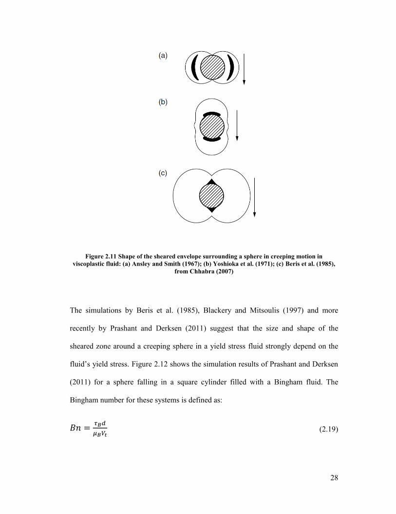
The simulations by Beris et al. (1985), Blackery and Mitsoulis (1997) and more
recently by Prashant and Derksen (2011) suggest that the size and shape of the
sheared zone around a creeping sphere in a yield stress fluid strongly depend on the
fluid’s yield stress. Figure 2.12 shows the simulation results of Prashant and Derksen
(2011) for a sphere falling in a square cylinder filled with a Bingham fluid. The
Bingham number for these systems is defined as:
𝐵𝑛 =𝜏𝐵𝑑
𝜇𝐵𝑉𝑡 (2.19)
29
As the Bingham number increases, unyielded zones (shown by black spots) expand
and shift closer to the particle surface. As a result, terminal settling velocity of the
particle decreases dramatically with increase of fluid yield stress (Prashant and
Derksen, 2011).
Figure 2.12 Yielded (white) and unyielded (black) regions for flow of a Bingham fluid around a
fixed sphere contained in a square cylinder with L/d=4 (Prashant & Derksen, 2011)
Although the numerical simulations described above provide valuable information on
the size and shape of the sheared region surrounding a falling particle, they suffer
from one important constraint: the assumption of creeping motion. Therefore, on a
30
practical level, one must resort to empirical correlations to predict the drag coefficient
(and particle fall velocity) for many scenarios.
The correlations can be divided into two different categories. The first category
includes the methods that introduce dimensionless numbers based on fluid models
(Bingham, Casson, and Herschel-Bulkley) and correlate 𝐶𝐷 with these parameters.
Andres (1961), du Plessis and Ansley (1967), Ansley and Smith (1967), Valentik and
Whitmore (1965) have published notable studies in this category. In the second
category, the definition of Reynolds number is modified in a way that the results of
viscoplastic settling tests coincide with the standard Newtonian drag curve. Attapatu
et al. (1995) and Chafe and du Bryan (2005) provide examples of this type of
correlation.
While 𝐶𝐷 is an important parameter, it has been proven to be particularly difficult to
calculate 𝑉𝑡 using these methods (Gumulya 2009), mainly because 𝑉𝑡 emerges in both
𝐶𝐷 and the modified Reynolds number and numerous iterations are required to obtain
an acceptable estimate of 𝑉𝑡. Furthermore, the modified Reynolds numbers are
commonly defined by “apparent viscosity” for viscoplastic fluids, which is a function
of applied shear rate, which is a function of velocity itself. These complications
reduce the chances of (a) convergence and (b) obtaining a reasonably accurate
prediction of 𝑉𝑡.
The prediction methods of Ansley and Smith (1967) from the first category and
Attapatu et al. (1995) from the second category are explained here so that the
complexities associated with these trial-and-error methods can be illustrated.
31
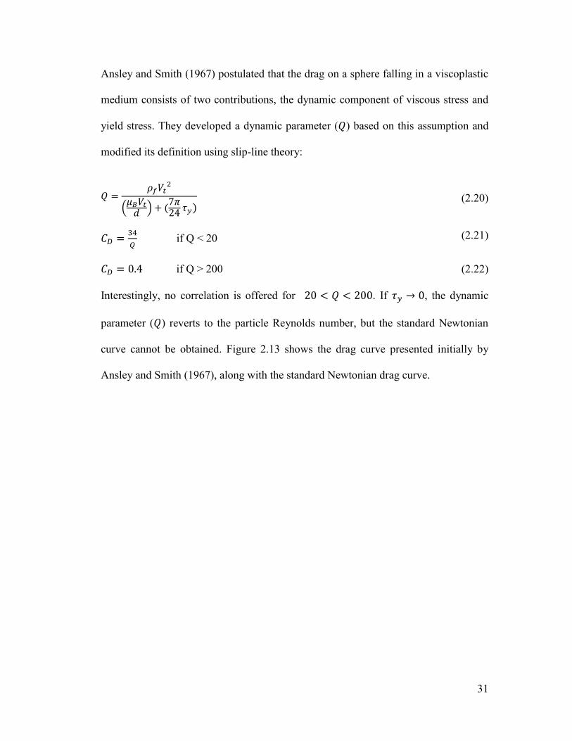
Ansley and Smith (1967) postulated that the drag on a sphere falling in a viscoplastic
medium consists of two contributions, the dynamic component of viscous stress and
yield stress. They developed a dynamic parameter (𝑄) based on this assumption and
modified its definition using slip-line theory:
𝑄 =𝜌𝑓𝑉𝑡
2
(𝜇𝐵𝑉𝑡
𝑑) + (
7𝜋24
𝜏𝑦) (2.20)
𝐶𝐷 =34
𝑄 if Q < 20 (2.21)
𝐶𝐷 = 0.4 if Q > 200 (2.22)
Interestingly, no correlation is offered for 20 < 𝑄 < 200. If 𝜏𝑦 → 0, the dynamic
parameter (𝑄) reverts to the particle Reynolds number, but the standard Newtonian
curve cannot be obtained. Figure 2.13 shows the drag curve presented initially by
Ansley and Smith (1967), along with the standard Newtonian drag curve.
32
Figure 2.13 Drag curve presented by Ansley and Smith (1967) for a sphere falling in a Bingham
fluid (from Saha et al. (1992))
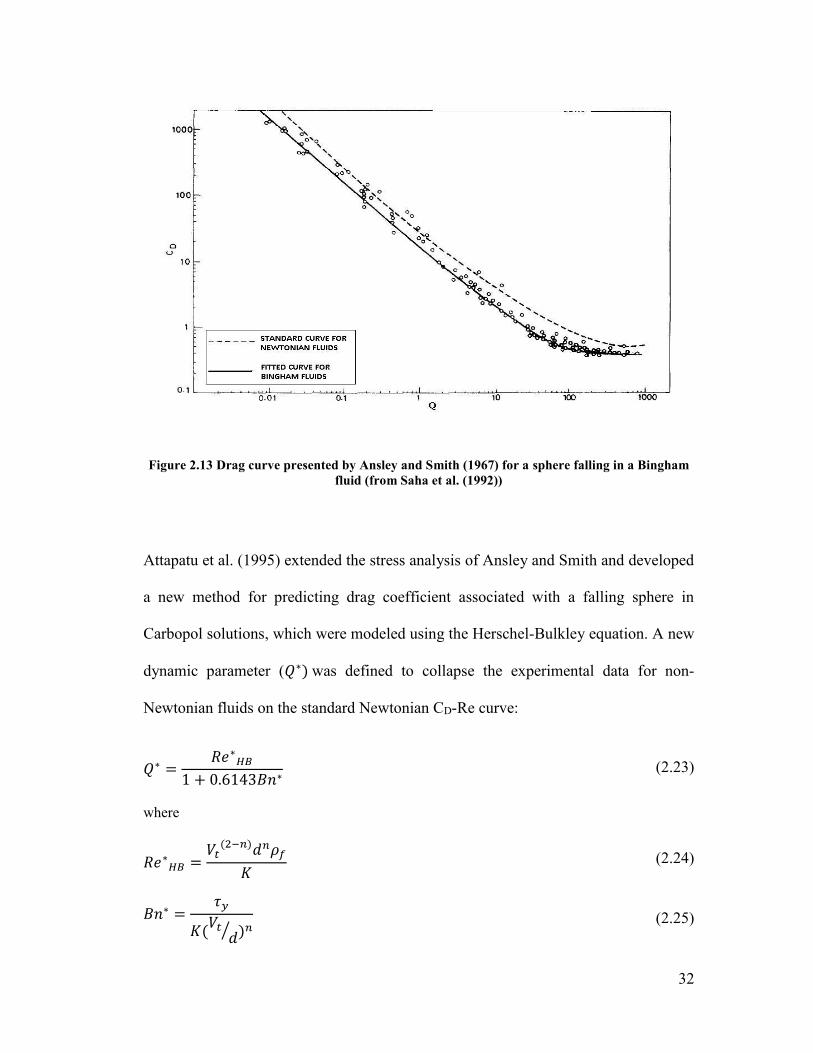
Attapatu et al. (1995) extended the stress analysis of Ansley and Smith and developed
a new method for predicting drag coefficient associated with a falling sphere in
Carbopol solutions, which were modeled using the Herschel-Bulkley equation. A new
dynamic parameter (𝑄∗) was defined to collapse the experimental data for non-
Newtonian fluids on the standard Newtonian CD-Re curve:
𝑄∗ =𝑅𝑒∗
𝐻𝐵
1 + 0.6143𝐵𝑛∗ (2.23)
where
𝑅𝑒∗𝐻𝐵 =
𝑉𝑡(2−𝑛)𝑑𝑛𝜌𝑓
𝐾 (2.24)
𝐵𝑛∗ =𝜏𝑦
𝐾(𝑉𝑡
𝑑⁄ )𝑛 (2.25)
33
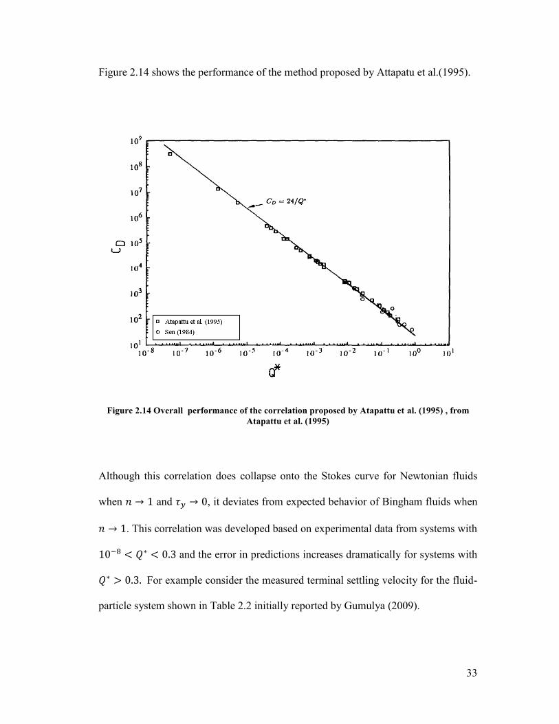
Figure 2.14 shows the performance of the method proposed by Attapatu et al.(1995).
Figure 2.14 Overall performance of the correlation proposed by Atapattu et al. (1995) , from
Atapattu et al. (1995)
Although this correlation does collapse onto the Stokes curve for Newtonian fluids
when 𝑛 → 1 and 𝜏𝑦 → 0, it deviates from expected behavior of Bingham fluids when
𝑛 → 1. This correlation was developed based on experimental data from systems with
10−8 < 𝑄∗ < 0.3 and the error in predictions increases dramatically for systems with
𝑄∗ > 0.3. For example consider the measured terminal settling velocity for the fluid-
particle system shown in Table 2.2 initially reported by Gumulya (2009).
34
Table 2.2 Physical properties and measured terminal settling velocity for a sphere falling in a
Herschel-Bulkley fluid, reported by Gumulya (2009)
𝑑 (m) 𝜌𝑓 (kg/m3) 𝜌𝑠 (kg/m3) 𝜏𝐻𝐵 (Pa) 𝐾 (𝑃𝑎. 𝑠𝑛) 𝑛 𝑉𝑡𝑚(m/s)
0.00635 998 8876 1.289 6.718 0.257 0.155
For 𝑉𝑡= 0.155 m/s, 𝑄∗ = 1.49. If one applies the correlation proposed by Attapatu et
al. (1995) the predicted fall velocity will be 𝑉𝑡𝑝 =1.31 m/s which is more than 8 times
larger than the measured velocity. Another limitation of this method is that it can only
be used for fluids with Herschel-Bulkley models.
Wilson et al. (2003) proposed a direct method for predicting terminal settling velocity
of spheres in viscoplastic fluids, which provided 𝑉𝑡 without iteration, but also utilized
the standard Newtonian drag curve. An apparent viscosity is calculated from the fluid
and particle properties and the terminal settling velocity is calculated for the sphere
falling in a Newtonian fluid with that apparent viscosity. In order to find the proper
apparent viscosity, the authors suggested a reference point on the fluid rheogram such
that the equivalent Newtonian viscosity at that point can be used and thus the non-
Newtonian settling data collapse on the Newtonian curve. The best reference point for
more than 180 data points was found to be 0.3𝜏, where 𝜏 is the mean surficial stress
of a falling sphere and can be calculated using Equation (2.12). This method provides
good predictions for cases where 𝑅𝑒∗ > 100 . In this region, (𝑅𝑒∗ > 100 ) the
average absolute error is 9.7% for 133 data points. Figure 2.15 shows the results of
Wilson et al.’s method.
35
Figure 2.15 Experimental fall velocity measurements reported by Wilson et al. (2003, 2004) and
shown on their standard Newtonian curve, with τref = 0.3��
There are two important limitations associated with this method. The predictions for
terminal settling velocity seem to deviate considerably from the Newtonian curve
when 𝑹𝒆∗<100. The average absolute error for predictions in this region is 75% for
62 data points. The other limitation of this method is that if, for a particular fluid-
particle system, the reference point of 0.3�� is less than yield stress of the fluid (𝝉𝒚),
there are no points on the rheogram to choose as the reference point; without a
reference point no apparent viscosity can be calculated and therefore no prediction of
terminal settling velocity can be made. Because of this constraint, the Wilson et al.
(2003) method is not universally applicable. The focus of the present study, as was
36
mentioned in Chapter 1, is to modify the Wilson et al. (2003) method to improve both
the accuracy of predictions and the range of applicability.
2.4 Wall effects
2.4.1 Newtonian medium
When a particle falls in a fluid in the presence of solid boundaries, it reaches a
stabilized velocity which is less than its terminal settling velocity in that fluid
(Rhodes, 2008). From an analytical point of view, the containing walls change the
boundary conditions needed to solve the equations of motion and the continuity
equation for the continuous phase (Clift et al., 1978). The physical explanation for
this phenomenon is that as the particle settles, an upward fluid displacement occurs.
As the particle-to-container diameter ratio increases, the upward velocity of the fluid
becomes significant (i.e. it can no longer be considered to be zero), which in turn
increases the drag force acting on the particle; thus the terminal settling velocity of
the particle is reduced. Figure 2.16 shows a schematic view of this mechanism. A
good understanding of this phenomenon is crucial in the design of settling
experiments and interpretation of results, and is therefore discussed in greater detail in
the following paragraphs.
37
Figure 2.16 Schematic view of hindering effect of container boundaries on settling velocity of a
single sphere in a Newtonian fluid
One can use a wall factor (𝑓𝑤) to relate the measured particle settling velocity (𝑉𝑚) to
the velocity of the same particle in an unbounded medium, i.e. the terminal settling
velocity (𝑉𝑡):
𝑓𝑤 =𝑉𝑚
𝑉𝑡 (2.26)
Based on this definition, 𝑓𝑤 can take a value between zero and unity. Other
definitions of wall factor have been used in the literature, including the ratio of drag
forces in bounded and unbounded media, the ratio of calculated viscosity using
Stokes formula in finite and infinite mediums and 1 𝑓𝑤⁄ (Chhabra, 2007). The velocity
ratio as shown in Equation (2.26) has been chosen to calculate 𝑓𝑤 by many
researchers (Chhabra, 2007).
38
For a rigid sphere falling axially in an incompressible Newtonian fluid in a cylindrical
tube, the wall factor 𝑓𝑤 is function of particle Reynolds number (𝑅𝑒𝑝) and sphere-to-
container diameter ratio (𝜆 =𝑑𝑝
𝐷⁄ )(Chhabra et al., 2003).
There are numerous correlations available to predict the wall factor 𝑓𝑤 for different
ranges of both 𝑅𝑒𝑝 and 𝜆. Chhabra et al. (2003) conducted an extensive review on
methods used to predict 𝑓𝑤 for the case of a single rigid sphere settling in a
Newtonian fluid in a cylindrical container. Their review showed that at very low or
very high 𝑅𝑒𝑝, the wall factor is a function of 𝜆 only, while at intermediate 𝑅𝑒𝑝, 𝑓𝑤 is
a function of both 𝑅𝑒𝑝 and 𝜆. The limiting values of particle Reynolds number for
each region (viscous, transition, and turbulent) are functions of sphere-to-container
diameter ratio. Based on a statistical analysis of 1260 data points collected from
several sources in the literature, Chhabra et al. (2003) selected the correlations which
gave predictions with the lowest maximum and average error in each region. Table
2.3 shows the preferred correlations and the range of applicability for each region.
39
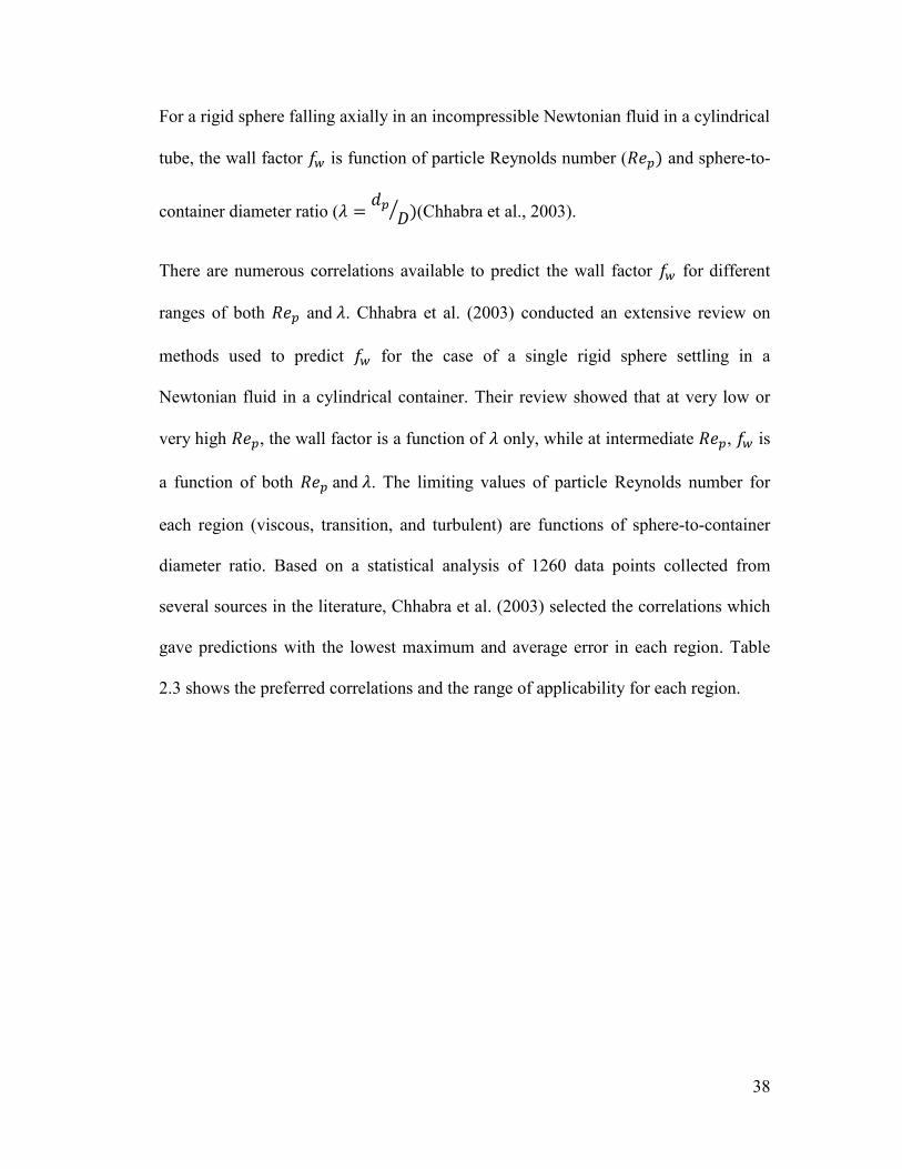
Table 2.3 Correlations for estimating wall effects for a particle settling in a Newtonian fluid
(Chhabra et al., 2003)
Source Correlation Range of
applicable 𝑅𝑒
Haberman
and Sayre
(1958) 𝑓𝑤 =
1 − 2.105𝜆 + 2.0865𝜆3 − 1.7068𝜆5 + 0.72603𝜆6
1 − 0.75857𝜆5
𝑅𝑒𝑝 < 0.027
for 𝜆 = 0.1
𝑅𝑒𝑝 < 0.04 for 𝜆 =
0.2
(Di Felice,
1996) 𝑓𝑤 = (
1 − 𝜆
1 − 0.33𝜆)𝜀 where 𝜀 =
3.3 + 0.085𝑅𝑒𝑝
0.1𝑅𝑒𝑝 + 1
0.027 < 𝑅𝑒𝑝 < 60
for 𝜆 = 0.1
0.04 < 𝑅𝑒𝑝 < 110
for 𝜆 = 0.2
Newton
(1863) 𝑓𝑤 = (1 − 𝜆2)(1 − 0.5𝜆2)0.5
𝑅𝑒𝑝 > 60 for 𝜆 =
0.1
𝑅𝑒𝑝 > 110 for 𝜆 =
0.2
2.4.2 Viscoplastic medium
For viscoplastic fluids, wall effects cannot be described using the wall factors
produced for Newtonian fluids, primarily because of the different flow field around
the moving particle (Chhabra, 2007). As was discussed earlier, the sheared zone
around the moving sphere has a finite radius and the fluid is undisturbed beyond that
radius. If the sheared region of fluid does not extend to the container walls, then the
measured terminal settling velocity will be equal to the “true” or unhindered settling
velocity (Carreau et al., 1997).
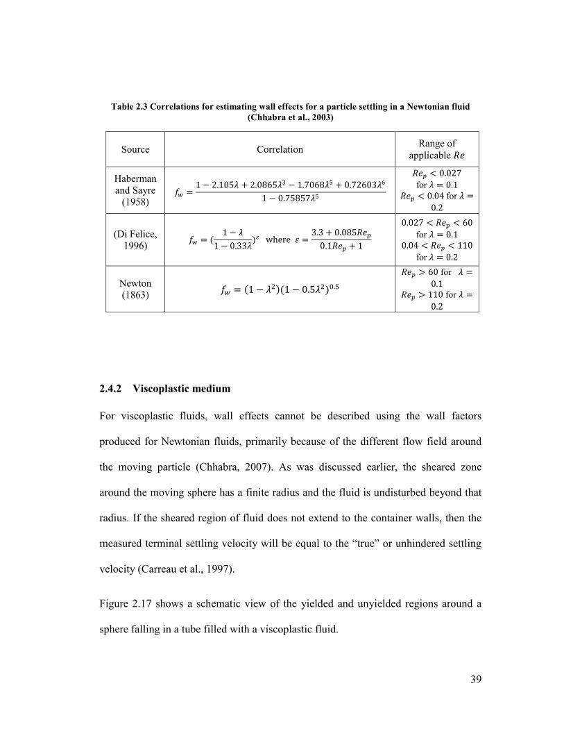
Figure 2.17 shows a schematic view of the yielded and unyielded regions around a
sphere falling in a tube filled with a viscoplastic fluid.
40
Figure 2.17 Schematic representation of the system of a sphere falling in a tube filled with a
viscoplastic medium. Both the outer shaded regions and dark interior regions are unyielded
(Beaulne and Mitsoulis, 1997)
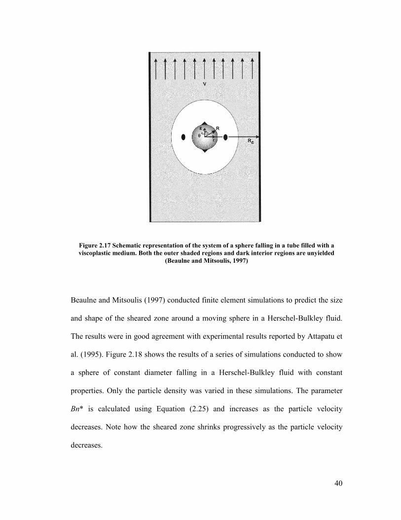
Beaulne and Mitsoulis (1997) conducted finite element simulations to predict the size
and shape of the sheared zone around a moving sphere in a Herschel-Bulkley fluid.
The results were in good agreement with experimental results reported by Attapatu et
al. (1995). Figure 2.18 shows the results of a series of simulations conducted to show
a sphere of constant diameter falling in a Herschel-Bulkley fluid with constant
properties. Only the particle density was varied in these simulations. The parameter
Bn* is calculated using Equation (2.25) and increases as the particle velocity
decreases. Note how the sheared zone shrinks progressively as the particle velocity
decreases.
41
Figure 2.18 Size of the sheared zone around a particle moving at different velocities in a
viscoplastic fluid (λ=1/3), from Beaulne and Mitsoulis (1997)
Chhabra (2007) conducted a comprehensive review of the investigations available in
the literature to estimate the radius of the sheared zone around the particle.
Experimental data and simulations for a wide range of system properties and
geometries were collected. It was concluded from experimental studies such as those
of Atapattu et al. (1990) and Atapattu et al. (1995) and from the simulations of Beris
et al. (1985) and Beaulne and Mitsoulis (1997) that the extent of the sheared region
radius is on the order of four times the sphere radius and decreases with decreasing
42
velocity. In a more recent study by Chafe and de Bryan (2005) a single sphere was
pulled through different bentonite clay suspensions and the radius of the sheared zone
was found to be twice the radius of the moving sphere in presence of significant wall
effects (𝜆 = 6).
Atapattu et al. (1986) proposed the following predictive expression for wall effects in
viscoplastic fluids:
𝑓𝑤
= 1 if 𝜆 < 𝜆𝑐𝑟𝑖𝑡 (2.27)
𝑓𝑤
= 1 − 1.7(𝜆 − 𝜆𝑐𝑟𝑖𝑡) if 𝜆 > 𝜆𝑐𝑟𝑖𝑡 (2.28)
𝜆𝑐𝑟𝑖𝑡 = 0.055 + 3.44𝑌𝐺 (2.29)
where 𝑌𝐺 is the yield-gravity parameter which can be calculated using Equation (2.5).
With the background provided in this chapter, one can conclude that a more
comprehensive and accurate method is required for the prediction of a sphere’s
terminal settling velocity in a viscoplastic fluid. In order to develop an improved
correlation that can cover a wider range of fluid-particle properties, it is critical to
conduct high quality experiments. The experiments conducted as part of the present
study are described in the following chapter.
43
3. Experimental method
3.1 Materials
3.1.1 Spheres
Several sizes of precision spheres made from different grades of steel, aluminum, and
ceramic (Penn Ball Bearing Co, Inc.) were used for settling experiments. Spheres
were reported to be smooth and have sphericity of more than 99%. The diameter was
reported by supplier with accuracy of 0.1%. The density of each set of spheres was
reported based on the grade of materials used. All the reported properties were
measured and confirmed during this study. Physical properties of the spheres are
listed in Table 3.1.
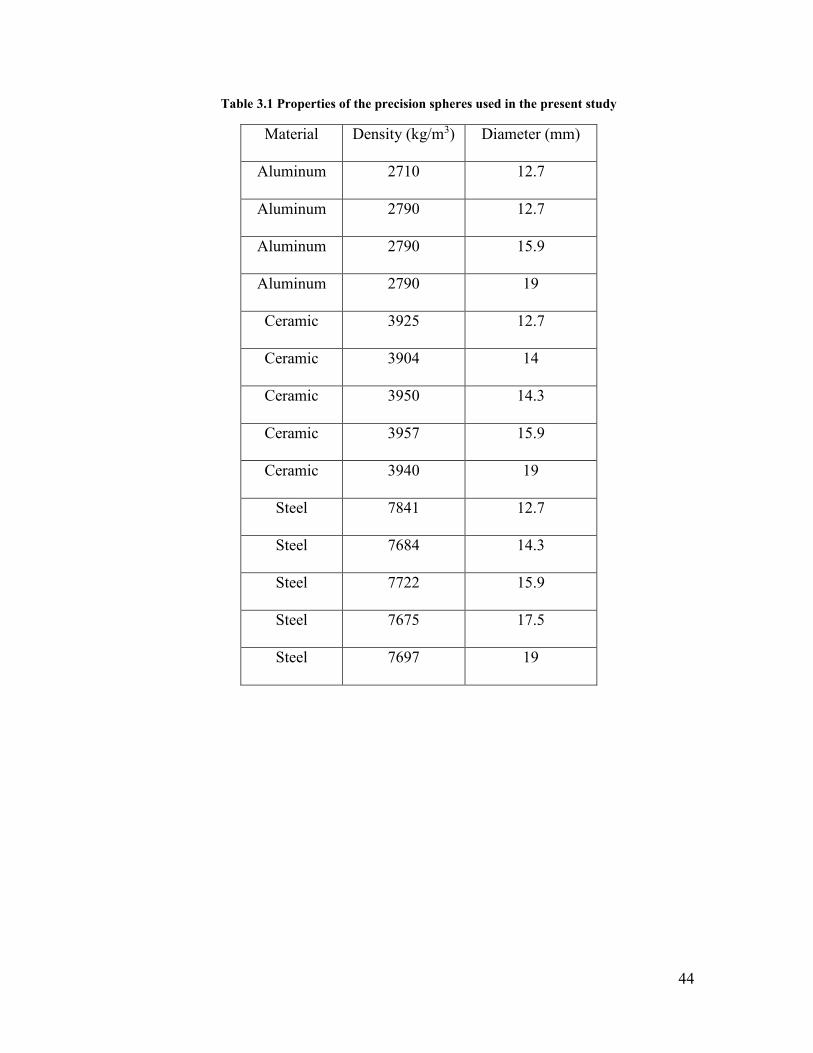
44
Table 3.1 Properties of the precision spheres used in the present study
Material Density (kg/m3) Diameter (mm)
Aluminum 2710 12.7
Aluminum 2790 12.7
Aluminum 2790 15.9
Aluminum 2790 19
Ceramic 3925 12.7
Ceramic 3904 14
Ceramic 3950 14.3
Ceramic 3957 15.9
Ceramic 3940 19
Steel 7841 12.7
Steel 7684 14.3
Steel 7722 15.9
Steel 7675 17.5
Steel 7697 19
45
3.1.2 Kaolinite
It was established in Chapter 2 that Kaolinite is a type of clay, often found in mining
operations and oil sands extraction, which can produce a viscoplastic fluid when
mixed with water. The Kaolinite in this study was supplied by Kentucky-Tennessee
Clay Company. According to the supplier, between 54% to 65% of particles have a
mean diameter less than 2 𝜇m, the density is 2650 kg/m3, and the pH is 6.5.
3.1.3 Corn syrup
A solution of corn syrup and tap water was used as the Newtonian fluid for settling
column calibration experiments. The corn syrup was provided by a local supplier
(Bakers Supreme) and the density was measured to be 1371 kg/m3.
3.2 Equipment
3.2.1 Settling column
A column with a circular cross section was used for settling experiments conducted as
part of the present study. A schematic view of this setup is shown in Figure 3.1. The
column is 1.5 m in length and 101.6 mm in diameter (i.d.). The settling column
consists of four main sections. The acrylic transparent section provides visual access
to a settling particle. The second section is used for Electrical Impedance
Tomography (EIT) measurements and consists of two sets of sensors located 40cm
from each other. At the very top part of the column, a frame, secured to the column
itself, holds in place the vacuum tube guide, which is used to hold the vacuum tube in
the dead-center of the column and just at the fluid free surface. The frame can be
removed for cleaning or sample collecting purposes. At the bottom of the apparatus, a
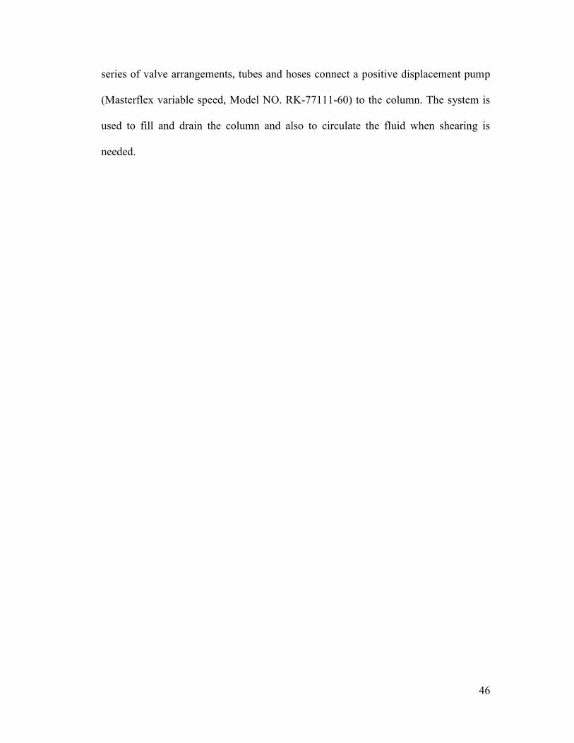
46
series of valve arrangements, tubes and hoses connect a positive displacement pump
(Masterflex variable speed, Model NO. RK-77111-60) to the column. The system is
used to fill and drain the column and also to circulate the fluid when shearing is
needed.
47
Figure 3.1 Schematic view of the settling apparatus
48
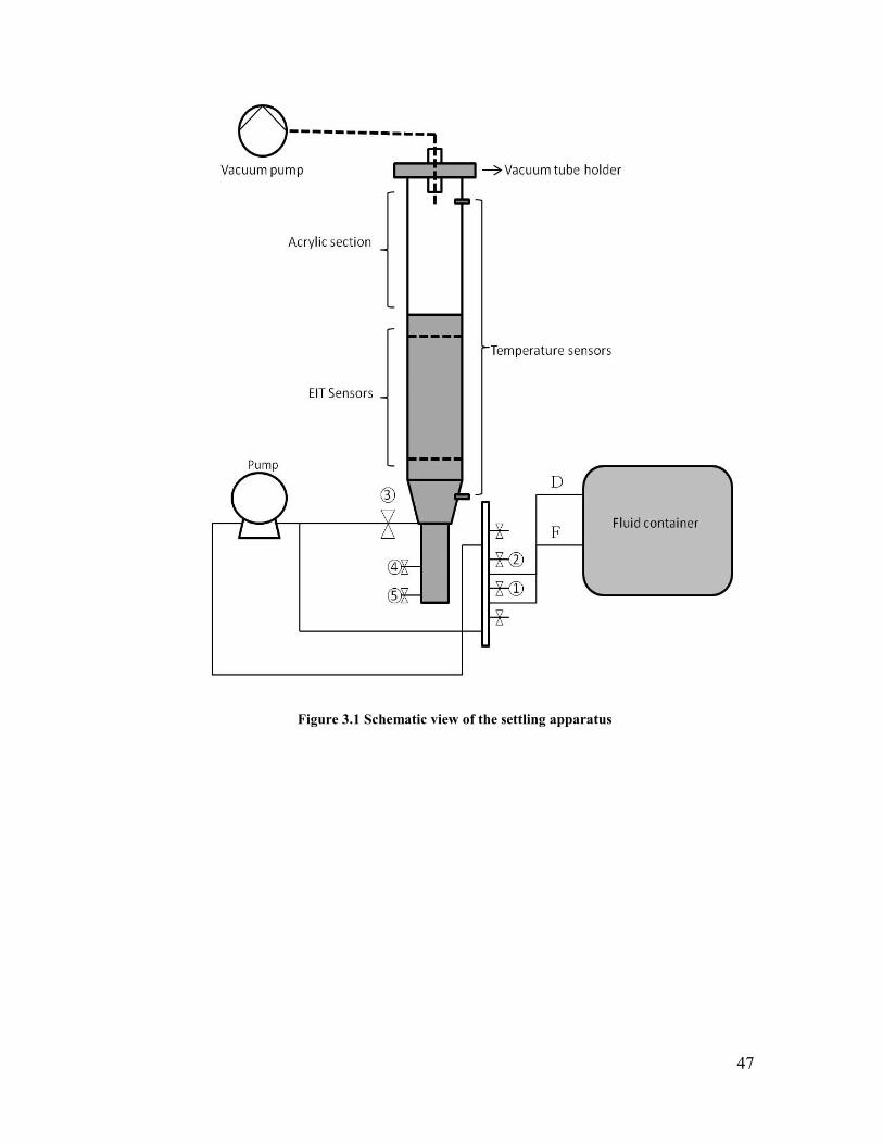
3.2.2 EIT sensors
The fall velocity of each particle tested in this study was measured using Electrical
Impedance Tomography sensors. There are two rows of sensors located within 40 cm
from each other and each row consists of 16 single electrodes arranged at equal
spacing around the circular pipe. A current is provided from an external source for an
initial pair of electrodes and the measured voltage from these two sensors and all the
other ones in the same row is recorded. Then the same current is provided for a
different pair and the same process is repeated. The recording of voltage responses
continues until all the sensors are covered and a full rotation of voltage measurements
is obtained. Each full set of voltage measurements, is translated to a full conductivity
map of the fluid disk in contact with the sensors (Brown, 2003). The thickness of this
disk is 5 mm and each full conductivity map is recorded as a “frame”.
Figure 3.2 Side view (left) and top view (right) of EIT sensor electrode arrangements
49
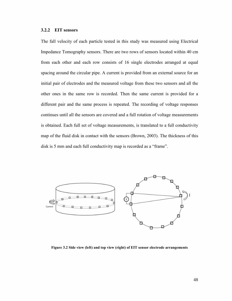
The electrode sensors are connected to the EIT z8000, a high speed electrical
impedance tomography data acquisition system, which can capture more than 1000
frames from 2×16 electrode sensors every second (z8000 EIT product sheet). The
data collection speed in this study covered a large range from 10 fps for creeping
particles to 825 fps for rapidly settling ones. The frequency of AC injecting current
was set at 80 kHz.
The instrument collects the voltage measurements form the sensors and reconstructs
the data to produce a conductivity map (Hashemi, 2013). The reconstrucion grid is
shown here as Figure 3.3.
Figure 3.3 EIT reconstruction grids
50
When an object with a different conductivity relative to the reference medium fluid
passes through, the conductivity in a series of pixels shown in Figure 3.3 changes.
The average conductivity of each plane at any moment is assigned to the frame
collected at that moment; therefore, by having a graph of average (plane) conductivity
versus number of frames, the precise moment of particle arrival can be determined.
Figure 3.4 shows the change in average conductivity caused by a passing aluminum
sphere. Two high peaks on the graph show that the particle has a higher conductivity
than the medium and by comparing the width of peaks it can be concluded that the
velocity of particle has remained constant from the first plane to the second one.
Figure 3.5 shows full conductivity maps of the first sensor plane, just before and just
at the time the particle reaches the plane.
In this study, the exact arrival time of the particle to the first and second plane is
observed, and the velocity is calculated by dividing the flight time of the particle by
the distance between the two sensor planes (40 cm).
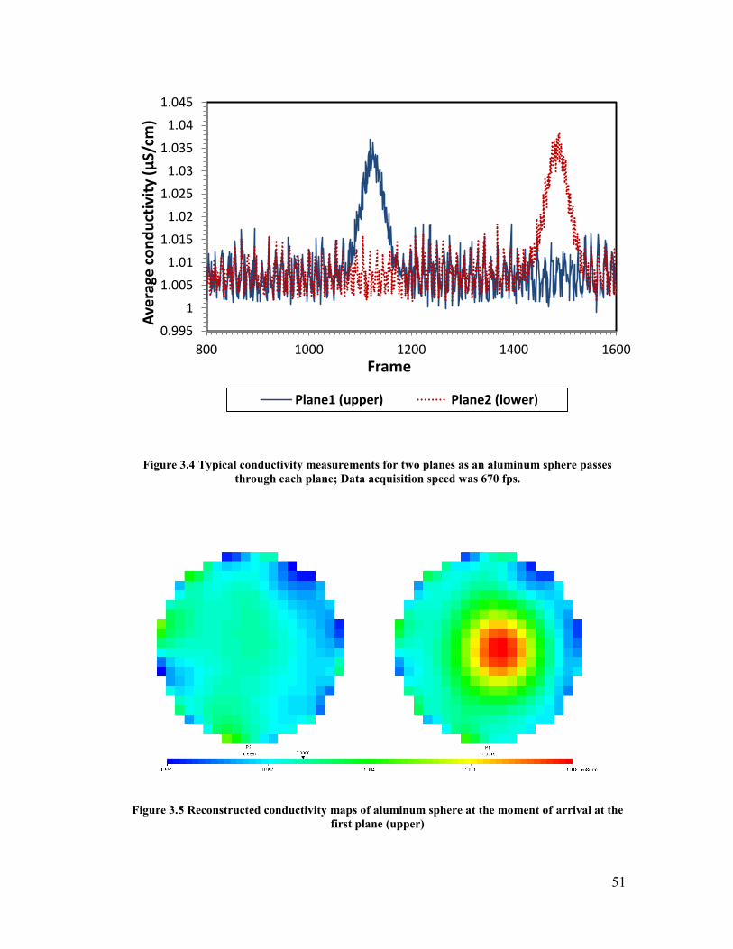
51
Figure 3.4 Typical conductivity measurements for two planes as an aluminum sphere passes
through each plane; Data acquisition speed was 670 fps.
Figure 3.5 Reconstructed conductivity maps of aluminum sphere at the moment of arrival at the
first plane (upper)
0.995
1
1.005
1.01
1.015
1.02
1.025
1.03
1.035
1.04
1.045
800 1000 1200 1400 1600
Ave
rage
co
nd
uct
ivit
y (µ
S/cm
)
Frame
Plane1 (upper) Plane2 (lower)
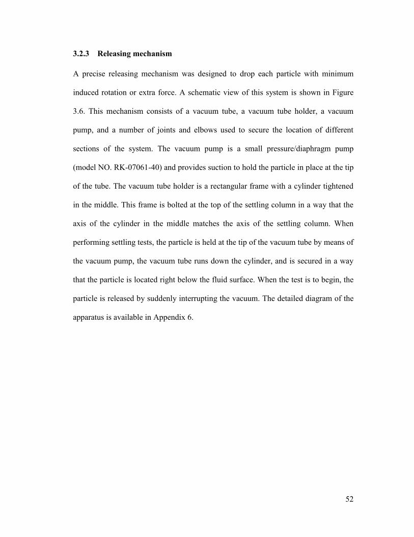
52
3.2.3 Releasing mechanism
A precise releasing mechanism was designed to drop each particle with minimum
induced rotation or extra force. A schematic view of this system is shown in Figure
3.6. This mechanism consists of a vacuum tube, a vacuum tube holder, a vacuum
pump, and a number of joints and elbows used to secure the location of different
sections of the system. The vacuum pump is a small pressure/diaphragm pump
(model NO. RK-07061-40) and provides suction to hold the particle in place at the tip
of the tube. The vacuum tube holder is a rectangular frame with a cylinder tightened
in the middle. This frame is bolted at the top of the settling column in a way that the
axis of the cylinder in the middle matches the axis of the settling column. When
performing settling tests, the particle is held at the tip of the vacuum tube by means of
the vacuum pump, the vacuum tube runs down the cylinder, and is secured in a way
that the particle is located right below the fluid surface. When the test is to begin, the
particle is released by suddenly interrupting the vacuum. The detailed diagram of the
apparatus is available in Appendix 6.
53
Figure 3.6 Schematic illustration of the releasing mechanism
3.2.4 Rheometer
All rheometry measurements were made using an ARG2 rheometer (TA instruments,
New Castle, DE, USA). There are various types of geometries available for this
instrument including concentric cylinder, cone and plate, and parallel plates. The
combination of magnetically levitating mechanism with traditional air-bearing
supposedly increases the accuracy of results in comparison to similar instruments.
ARG2 can provide angular velocities between 1.4E-9 rad/s to 300 rad/s and torques
between 0.03 μN. m to 200 mN.m with a resolution of 0.1 nN.m. The rheometer is
connected to a temperature control unit that utilizes deionized water as the circulating
cooling fluid.
The cone and plate geometry is used for majority of rheology measurements in this
study. The diameter of the cone is 60mm with an angle of 2.0 degrees. The tip of the
54
cone is truncated and a gap of 58 𝜇m between the cone tip and the peltier plate is set
before each experiment.
3.2.5 Mixer
A heavy duty mixer from the EUROSTAR series of IKA mixers (model NO. S-
50705-30) was used to prepare Kaolinite-water mixtures. The overhead motor was
able to provide a range of mixing speeds between 30 and 2000 rpm, a maximum
torque of 60 N.cm, and a maximum input power of 0.19 hp.
A 3-blade axial flow impeller (Lightning A315) was used to stir the mixture. The
approximate dimensions of the mixing apparatus are available in Appendix 6.
3.3 Procedures
3.3.1 Preparation of corn syrup solutions
The general procedure is as follows:
1. Weigh the required amount of tap water and place it in mixing container.
2. Start the mixer on 140 rpm.
3. Weigh the required amount of corn syrup and gradually add it to the solution.
Increase the mixing velocity at each step to have a full vortex all the time.
4. Let the mixing continue for a minimum of 15 minutes after the last addition. Once
the solution appears to be homogenous, stop the mixer and place the mixing
container near the column.
55
3.3.2 Preparation of Kaolinite-water mixture
A standard procedure developed by Rahman (2011) was followed to prepare the
Kaolinite-water mixtures. The purpose of this procedure is to first ensure the
suspension is entirely homogenous, and then to eliminate or minimize the shear-
dependent sensitivities of the suspension. The total volume of fluid required for the
settling column is 17L.
The procedure is as follows:
1. Weigh the required amount of tap water and place it in the mixing container.
2. Adjust the impeller height so that the distance between the impeller tip and the
bottom of the container is half the container diameter.
3. Start the mixer on the lowest mixing speed that produces a vortex at the center.
For water, this mixing speed was 140 rpm.
4. Gradually add the required amount of Kaolinite to the mixture. A 500 mL beaker
was used to weigh and add Kaolinite to the mixture in multiple steps. Increase the
rpm after each step to get a full vortex.
5. Add required amount of CaCl2.2H2O such that CaCl2.2H2O: Kaolinite (w/w)
=0.001.
6. Continue mixing at the minimum velocity that provides a full vortex for an hour.
7. Collect 3 mL of sample by means of a syringe for an early rheometry test.
8. If the rheological properties of the fluid are to be manipulated for the settling
tests, use 0.25 M NaOH to adjust the pH. Continue mixing for an hour after the
last addition step.
56
3.3.3 Fluid density measurements
The general procedure is as follows:
1. Use a syringe to collect a 10 ml sample of fluid for density measurements.
2. Ensure the pycnometer is completely dry. Record the weight of dry pycnometer
(𝑊𝑝).
3. Inject 10 ml of deionized water into the pycnometer and secure the thermometer
at the top.
4. Dry the outer surface of pycnometer with a paper towel and record the weight
(𝑊𝑤).
5. Drain the pycnometer and repeat the same procedure (steps 2 to 4) for sample
fluid (𝑊(𝑝+𝑠)).
6. Calculate the specific gravity of the sample fluid using:
𝑆𝐺 = (𝑊(𝑝+𝑠) − 𝑊(𝑝))
(𝑊𝑤 − 𝑊(𝑝)) (3.1)
The density of the fluid can be calculated by multiplying SG by the density of
deionized water at the temperature of the experiment.
3.3.4 EIT operation
In this study, a wide range of particle fall velocities between 3 mm/s to 1.8 m/s was
measured. To guarantee that the z8000 system will be able to track the particle
movement from the first sensor to the second, the proper data collection speed must
be selected. For the calibration phase, the velocity of a sphere in a Newtonian fluid
57
was estimated using the Wilson et al. (2003) method. The arrival time of a chosen
particle to each sensor was then calculated based on this estimation and the EIT data
collection speed was set so that this time of flight could be easily tracked.
There are two categories for data collection on the z8000 instrument. The first
category is an “offline” measurement which is suited for high speed data collection
with higher sensitivity to conductivity change, and the second category is online
measurement which is more appropriate for lower velocities. In the z8000 operating
software, there are two parameters that manipulate measurement speed: “waiting
time” controls the data collection speed for offline mode and “sample interval (ms)”
manages the speed in online measurements. The total time required for a sphere to fall
can be calculated and the measurement method/speed was selected to cover that time.
3.3.5 Settling tests
There is always a possibility for excessive humidity, rust or dust inside the column.
To ensure that the fluid in the column is still homogenous, before filling the column
for settling experiment, the new fluid will be circulated several times in the system.
The procedure for performing a settling test on the settling column requires two
operators. See Figure 3.1 for visual references. The general procedure is as follows:
1. Locate the filling tube (F) in the container.
2. In filling situation, Valves NO. 1, 4, 5 must be closed and Valve 3 should be open.
3. Set the pump speed on 3 rpm. Start the pump in forward direction.
4. Wait for the fluid to reach the top of the column and stop the pump when the fluid
level has reached the mark on the top.
58
5. Wait for two minutes and inspect different parts of the setup to detect any possible
leaks caused by loose joints.
6. Drain the column. Locate the draining tube in the container. In draining mode,
Valves 4, 5 must be closed and 1, 2, 3 should be open.
7. Start the pump with the same speed (3 rpm) in reverse direction.
8. Repeat steps 5 to 12 three times. Then collect a 3 ml sample from the container
for rheometry measurements.
9. Set the proper method/speed for EIT sensors.
10. Fill the column based the procedure explained in steps 1 to 5.
11. Close the Valve NO. 3. This valve connects the pump to the column. If it is left
open the fluid will return to the fluid container.
12. Start the vacuum pump and Operator 1 climbs the ladder with desired spheres.
13. Operator 1 places the sphere at the tip of the vacuum tube and secures it on the
holder frame.
14. Operator 2 starts the EIT, performs the basic calibrations and takes reference
measurements.
15. When everything is set, Operator 1 interrupts the vacuum system using the outlet.
Operator 2, at the same time, starts acquiring data on the software.
16. During the settling, the trajectory of the sphere will be monitored by the
operators. The settling experiment is repeated (at least four times) at identical
conditions and an average of measured velocities are reported.
17. After obtaining at least four data points, the procedure will be repeated with a
different sphere as needed.
59
3.3.6 Kaolinite-water suspension rheometry
It was concluded in Chapter 2 that the cone-and-plate geometry is appropriate for
rheometry measurements on Kaolinite-water mixtures at low shear rates. At different
times during the settling experiments, 3 mL samples of fluid were collected from top
and bottom of the column by means of a syringe and tested to ensure rheology
properties of the fluid are stable. The procedure for low shear rheometry with the
AR-G2 rheometer is as follows:
1. Before each test, it is crucial to provide enough air pressure to the motor to ensure
that leveling, rotations and all the mechanical settings of the device can be
properly controlled. The optimum pressure for this device is 30 psi.
2. Before turning the device on, any new geometry or locking piece should be
detached. The moment the device starts, it attempts to recognize the geometry and
reload the details from its library. If the geometry is new, it tries to perform zero
gap and all other procedures to record the properties of this new piece. These
procedures at this stage can damage the device since it cannot be stopped or
controlled.
3. After the instrument is safely on and the spindle is rotating freely, the software can
be started and connected to the device. From the software menu on the left
“calibration” and on the top right the option of Instrument should be selected. The
first option on the menu is “inertia”. At this point, no geometry should be attached.
Inertia calibration takes about 30 seconds and at the end of it a single number is
reported. This number should be around 18.8 𝜇𝑁. 𝑚. 𝑠2 . The instrument uses this
60
as a correction factor for torque response measurements. It is recommended that
this type of calibration is performed at least once every three months.
4. After inertia calibration, the chosen geometry should be attached. All geometries
have a serial number written at the part where they are connected to the
instrument. After attaching it to the device safely, “smart swap” option must be
chosen. The geometry will rotate and the device will read the serial number and
reload the information on the attached geometry from its library. After this, it is
important to turn the smart swap off because the device keeps reading the serial
number and reloading everything even during the tests.
5. The only control parameter here is the precision. For these tests, number of
iterations was set on 2, as was advised by the training agent from the company.
This calibration takes 10 minutes and it is recommended to be performed each
time the geometry is detached and attached again. In this calibration, the device
rotates the geometry with a large range of velocities and records the torque
response of the geometry when no fluid is being tested. These torque responses
produce a reference map for the device which is used to correct torque
measurements.
6. After the rotational mapping is complete, “zero gap” calibration should be
performed. In this type of calibration, the device lowers slowly and marks the
point where the cone tip touches the plate. That reference point is used later to set
the dimensions at which measurements are made. When this has been completed,
the cone/spindle should be raised so that the rheometer can be loaded.
61
7. The last step before setting the specific procedure of the experiment is to set the
temperature. To achieve best results in terms of temperature stability, the sample is
loaded first and then the desired temperature is set. This allows the sample
temperature to stabilize at the same time that the instrument temperature is being
stabilized. For loading, 2 ml of fluid was collected by means of a syringe and put
carefully at the center of the plate. From the environment menu the desired
temperature can be entered now.
8. At this point all necessary calibrations have been performed and the device is
ready to receive details of the desired experimental procedure. Two steps were
defined for each test. The first step (conditioning) has two control parameters;
temperature and soaking time. The temperature is inherited from the setting in step
7, and the soaking time was set to be 20 seconds.
9. The second step is the main test. There are several options available as control
parameters. Spindle velocity was chosen. There are critical parameters that should
be calculated before setting the test. The details of these calculations have been
discussed in Chapter 2.
10. Start the experiment.
11. After the test is over, geometry should be raised to the “loading gap”, detached and
washed. The data will be transferred to Excel sheets for analysis.
62
3.3.7 Additional shearing procedure for highly-concentrated suspensions
The procedure for shearing the non-Newtonian fluids inside the column is as follows:
1. Fill the column following Steps 1 to 4 as described in Section 3.3.5.
2. Relocate the container and attach tubes to the bottom of the column.
3. Open Valves NO.4, 5, 3, 2 and close the Valve NO.1.
4. Wait until the container is almost half full. Then start the pump with 3 rpm
speed in forward direction. This way, the fluid is automatically circulated
through the column. Let the pump run for 10 minutes.
63
4. Results and Discussion
4.1 Settling tests: Newtonian fluids
The first phase of this study includes measurement of terminal settling velocity of
spheres in Newtonian fluids to calibrate the apparatus and develop the experimental
methodology. The settling column and particles along with primary procedures for
preparations have been introduced in the previous chapter. In order to produce
repeatable results, there are several parameters that have to be carefully monitored
and controlled during the experiment. As was mentioned in Chapter 2, terminal
settling velocity is the stabilized velocity of a single particle, falling in a stagnant and
infinite fluid. In order to ensure that the measured velocity of each sphere in the
settling column is in fact “terminal settling velocity” of that particle in the fluid, two
important conditions should apply:
The particle should reach a constant velocity before measurement begins,
which means that the observed velocity must be the same in both planes.
The sphere must have a straight trajectory, and fall at the center of the
column because the direct distance between two rows of sensors is used to
calculate velocity. Also, if the sphere is closer to the wall at different
locations along its trajectory, the wall effects will be important.
With the aim of designing the settling experiments such that these conditions are met,
a series of calibration tests were conducted.
A solution of corn syrup-water was prepared and used as the Newtonian fluid and
several spheres with different densities and diameters were used to perform settling
64
tests in low Reynolds numbers. For higher Reynolds numbers, tap water was used as
the Newtonian fluid. As was mentioned in Chapter 3, each test was repeated at least
four times and an average of recorded velocities was reported as the final result.
Transparency of corn syrup solutions and water made it possible to monitor the
trajectory of the sphere and ensure a relatively straight falling path. The settling tests
with visible inclined trajectories were discarded. In addition to that, the location of
sphere in each EIT plane was checked to confirm the straight trajectory in non-
transparent parts of the settling column. In cases where the sphere did not follow a
straight path because of error in the releasing process, the experiment was repeated.
Figure 4.1 shows examples of EIT results for settling tests with straight and angled
trajectories.
Figure 4.1 Sample conductivity maps for settling tests showing straight particle trajectory (left)
and angled particle path (right)
65
The particle must also reach a steady state velocity before any measurement is made.
In order to confirm the constancy of velocity at both measurement planes, the width
of the conductivity interruption curves was compared; identical curves meant constant
velocity. Figure 4.2 shows the conductivity curves for sphere (a) falling with constant
velocity and sphere (b) which hasn’t reached its stabilized settling velocity yet.
Figure 4.2 Sample of plane averaged conductivity measurements for settling tests with (a) a 12.7
mm aluminum sphere that has reached its terminal settling velocity and (b) an accelerating
12.7mm steel sphere
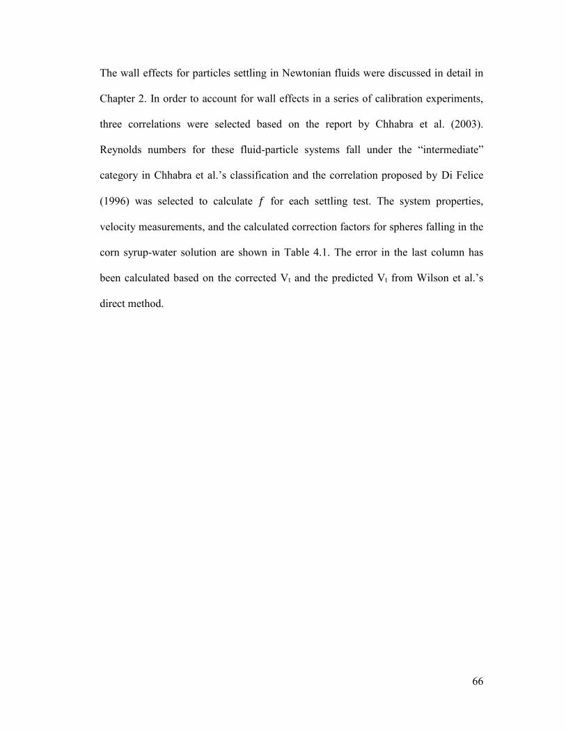
66
The wall effects for particles settling in Newtonian fluids were discussed in detail in
Chapter 2. In order to account for wall effects in a series of calibration experiments,
three correlations were selected based on the report by Chhabra et al. (2003).
Reynolds numbers for these fluid-particle systems fall under the “intermediate”
category in Chhabra et al.’s classification and the correlation proposed by Di Felice
(1996) was selected to calculate 𝑓 for each settling test. The system properties,
velocity measurements, and the calculated correction factors for spheres falling in the
corn syrup-water solution are shown in Table 4.1. The error in the last column has
been calculated based on the corrected Vt and the predicted Vt from Wilson et al.’s
direct method.
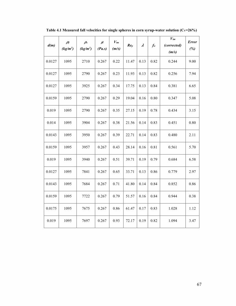
67
Table 4.1 Measured fall velocities for single spheres in corn syrup-water solution (CV=26%)
d(m) 𝜌f
(kg/m3)
𝜌s
(kg/m3)
𝜇
(Pa.s)
Vtm
(m/s) Rep 𝜆 fw
Vtm
(corrected)
(m/s)
Error
(%)
0.0127 1095 2710 0.267 0.22 11.47 0.13 0.82 0.244 9.00
0.0127 1095 2790 0.267 0.23 11.93 0.13 0.82 0.256 7.94
0.0127 1095 3925 0.267 0.34 17.75 0.13 0.84 0.381 6.65
0.0159 1095 2790 0.267 0.29 19.04 0.16 0.80 0.347 5.08
0.019 1095 2790 0.267 0.35 27.15 0.19 0.78 0.434 3.15
0.014 1095 3904 0.267 0.38 21.56 0.14 0.83 0.451 0.80
0.0143 1095 3950 0.267 0.39 22.71 0.14 0.83 0.480 2.11
0.0159 1095 3957 0.267 0.43 28.14 0.16 0.81 0.561 5.70
0.019 1095 3940 0.267 0.51 39.71 0.19 0.79 0.684 6.58
0.0127 1095 7841 0.267 0.65 33.71 0.13 0.86 0.779 2.97
0.0143 1095 7684 0.267 0.71 41.80 0.14 0.84 0.852 0.86
0.0159 1095 7722 0.267 0.79 51.57 0.16 0.84 0.944 0.38
0.0175 1095 7675 0.267 0.86 61.47 0.17 0.83 1.028 1.12
0.019 1095 7697 0.267 0.93 72.17 0.19 0.82 1.094 3.47
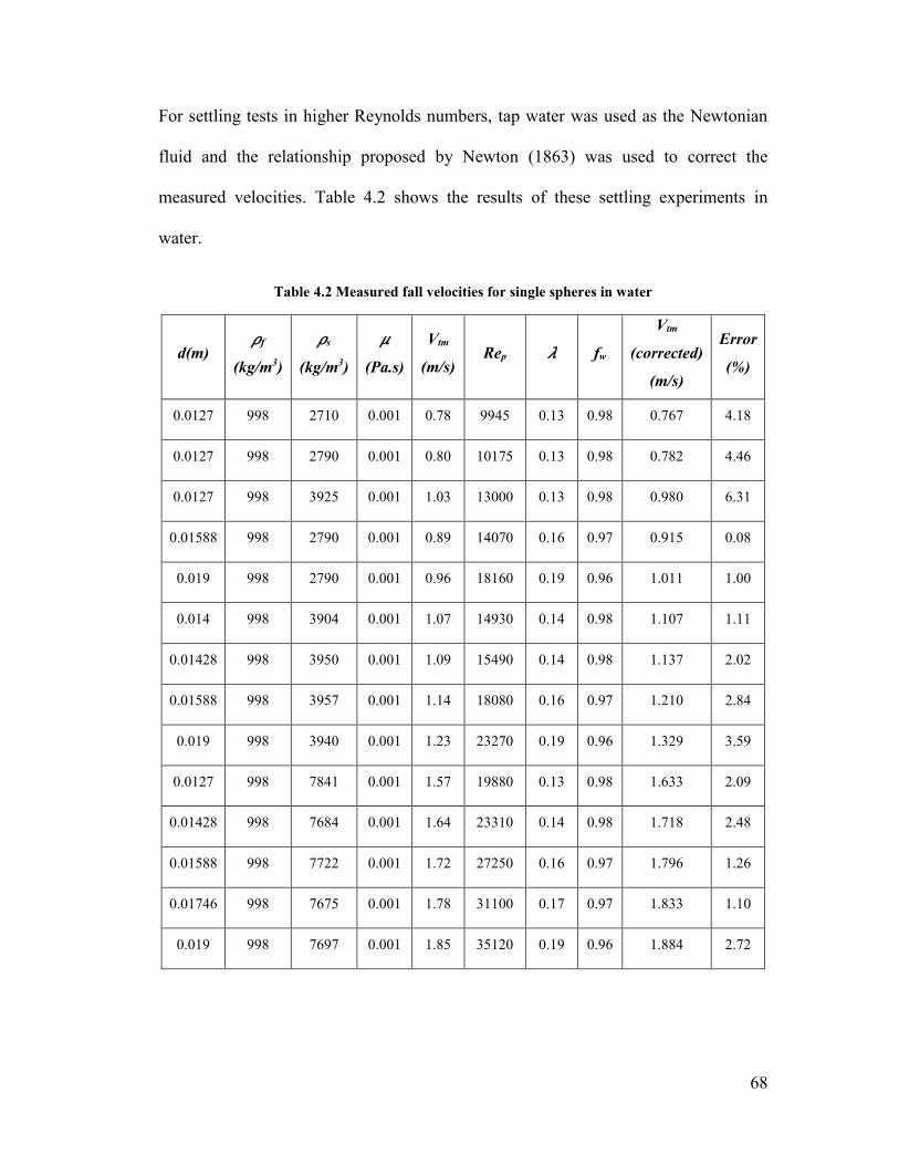
68
For settling tests in higher Reynolds numbers, tap water was used as the Newtonian
fluid and the relationship proposed by Newton (1863) was used to correct the
measured velocities. Table 4.2 shows the results of these settling experiments in
water.
Table 4.2 Measured fall velocities for single spheres in water
d(m) 𝜌f
(kg/m3)
𝜌s
(kg/m3)
𝜇
(Pa.s)
Vtm
(m/s) Rep 𝜆 fw
Vtm
(corrected)
(m/s)
Error
(%)
0.0127 998 2710 0.001 0.78 9945 0.13 0.98 0.767 4.18
0.0127 998 2790 0.001 0.80 10175 0.13 0.98 0.782 4.46
0.0127 998 3925 0.001 1.03 13000 0.13 0.98 0.980 6.31
0.01588 998 2790 0.001 0.89 14070 0.16 0.97 0.915 0.08
0.019 998 2790 0.001 0.96 18160 0.19 0.96 1.011 1.00
0.014 998 3904 0.001 1.07 14930 0.14 0.98 1.107 1.11
0.01428 998 3950 0.001 1.09 15490 0.14 0.98 1.137 2.02
0.01588 998 3957 0.001 1.14 18080 0.16 0.97 1.210 2.84
0.019 998 3940 0.001 1.23 23270 0.19 0.96 1.329 3.59
0.0127 998 7841 0.001 1.57 19880 0.13 0.98 1.633 2.09
0.01428 998 7684 0.001 1.64 23310 0.14 0.98 1.718 2.48
0.01588 998 7722 0.001 1.72 27250 0.16 0.97 1.796 1.26
0.01746 998 7675 0.001 1.78 31100 0.17 0.97 1.833 1.10
0.019 998 7697 0.001 1.85 35120 0.19 0.96 1.884 2.72
69
Figure 4.3 shows the corrected terminal settling velocities on the standard Newtonian
curve.
Figure 4.3 Terminal settling velocities corrected for wall effects; tests conducted with Newtonian
fluids
4.2 Settling tests: Kaolinite-water suspensions
Settling experiments were performed on more than 100 different fluid-particle
systems, using several different Kaolinite-water mixtures prepared based on the
procedures explained in Chapter 3, along with 14 spheres with different sizes and
densities. The yield-gravity parameter 𝑌𝐺 for fluid-particle systems in these
experiments varied from 0.0058 to 0.073. The correlation proposed by Atapattu et al.
(1986) for wall effect is based on the systems with 0.0091 < 𝑌𝐺< 0.058 and therefore
covers a large portion of the experiments done in this study. Less than 13% of the
0.1
1
10
1 10 100 1000 10000
Vt/
V*
Re*
Standard Newtonian curve
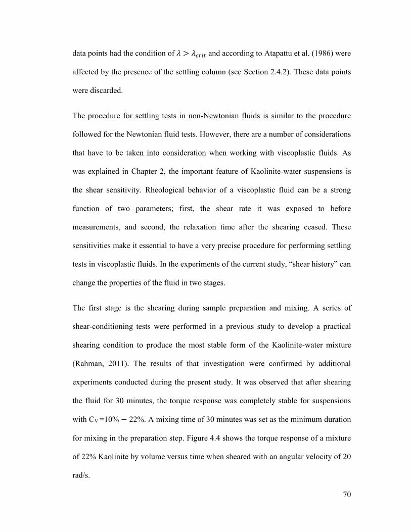
70
data points had the condition of 𝜆 > 𝜆𝑐𝑟𝑖𝑡 and according to Atapattu et al. (1986) were
affected by the presence of the settling column (see Section 2.4.2). These data points
were discarded.
The procedure for settling tests in non-Newtonian fluids is similar to the procedure
followed for the Newtonian fluid tests. However, there are a number of considerations
that have to be taken into consideration when working with viscoplastic fluids. As
was explained in Chapter 2, the important feature of Kaolinite-water suspensions is
the shear sensitivity. Rheological behavior of a viscoplastic fluid can be a strong
function of two parameters; first, the shear rate it was exposed to before
measurements, and second, the relaxation time after the shearing ceased. These
sensitivities make it essential to have a very precise procedure for performing settling
tests in viscoplastic fluids. In the experiments of the current study, “shear history” can
change the properties of the fluid in two stages.
The first stage is the shearing during sample preparation and mixing. A series of
shear-conditioning tests were performed in a previous study to develop a practical
shearing condition to produce the most stable form of the Kaolinite-water mixture
(Rahman, 2011). The results of that investigation were confirmed by additional
experiments conducted during the present study. It was observed that after shearing
the fluid for 30 minutes, the torque response was completely stable for suspensions
with CV =10% − 22%. A mixing time of 30 minutes was set as the minimum duration
for mixing in the preparation step. Figure 4.4 shows the torque response of a mixture
of 22% Kaolinite by volume versus time when sheared with an angular velocity of 20
rad/s.
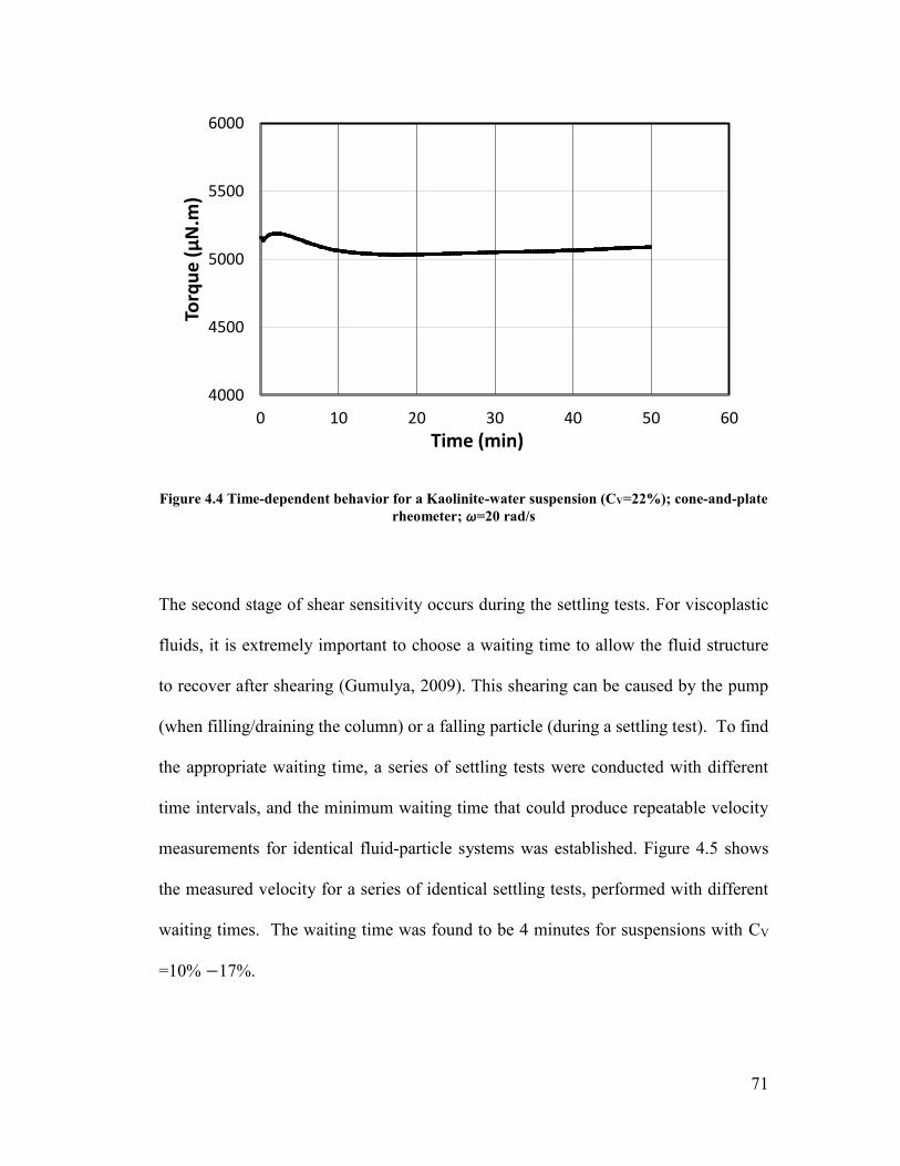
71
Figure 4.4 Time-dependent behavior for a Kaolinite-water suspension (CV=22%); cone-and-plate
rheometer; 𝜔=20 rad/s
The second stage of shear sensitivity occurs during the settling tests. For viscoplastic
fluids, it is extremely important to choose a waiting time to allow the fluid structure
to recover after shearing (Gumulya, 2009). This shearing can be caused by the pump
(when filling/draining the column) or a falling particle (during a settling test). To find
the appropriate waiting time, a series of settling tests were conducted with different
time intervals, and the minimum waiting time that could produce repeatable velocity
measurements for identical fluid-particle systems was established. Figure 4.5 shows
the measured velocity for a series of identical settling tests, performed with different
waiting times. The waiting time was found to be 4 minutes for suspensions with CV
=10% −17%.
4000
4500
5000
5500
6000
0 10 20 30 40 50 60
Torq
ue
(µ
N.m
)
Time (min)
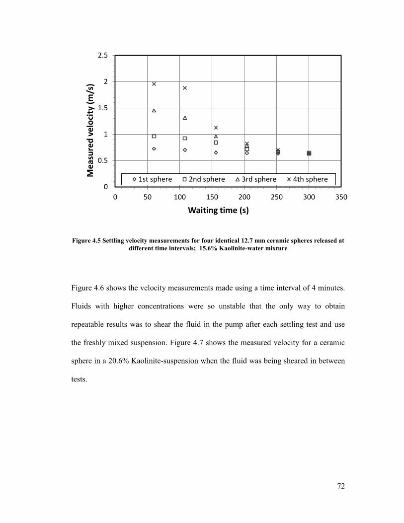
72
Figure 4.5 Settling velocity measurements for four identical 12.7 mm ceramic spheres released at
different time intervals; 15.6% Kaolinite-water mixture
Figure 4.6 shows the velocity measurements made using a time interval of 4 minutes.
Fluids with higher concentrations were so unstable that the only way to obtain
repeatable results was to shear the fluid in the pump after each settling test and use
the freshly mixed suspension. Figure 4.7 shows the measured velocity for a ceramic
sphere in a 20.6% Kaolinite-suspension when the fluid was being sheared in between
tests.
0
0.5
1
1.5
2
2.5
0 50 100 150 200 250 300 350
Me
asu
red
ve
loci
ty (
m/s
)
Waiting time (s)
1st sphere 2nd sphere 3rd sphere 4th sphere
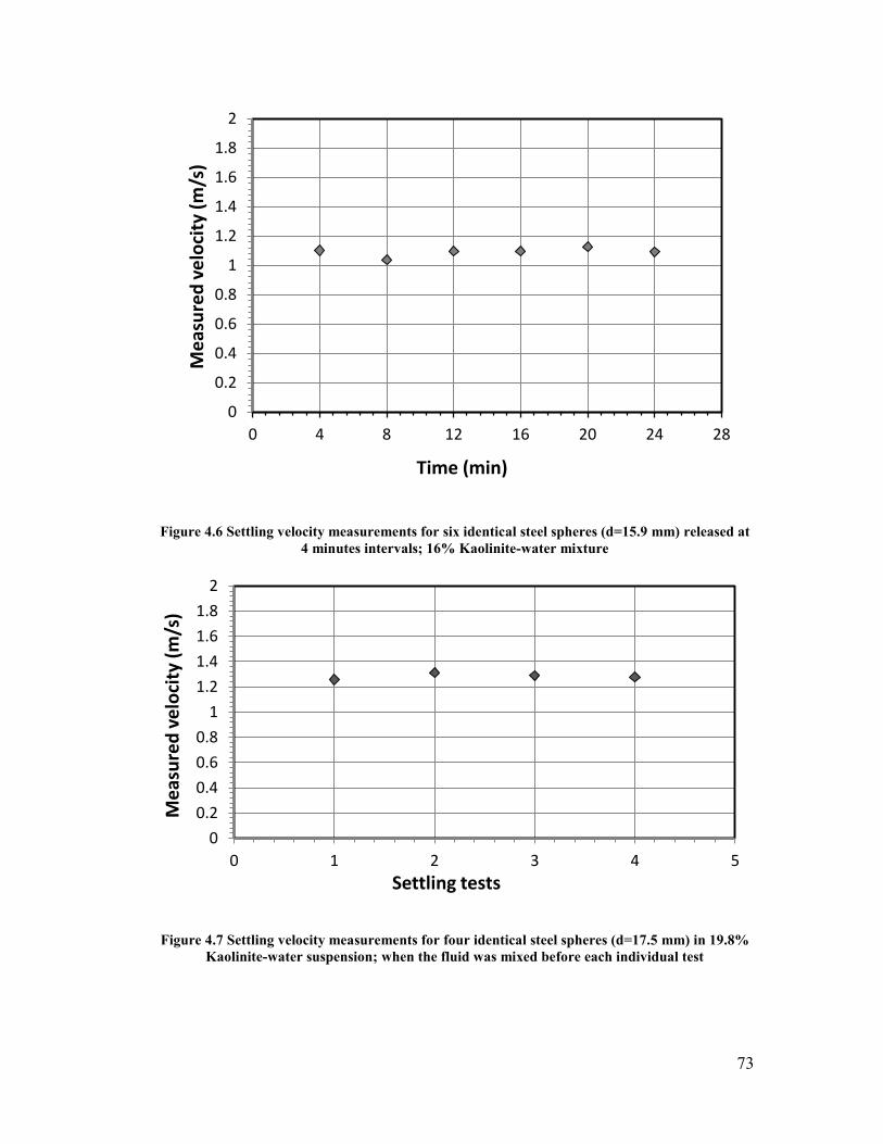
73
Figure 4.6 Settling velocity measurements for six identical steel spheres (d=15.9 mm) released at
4 minutes intervals; 16% Kaolinite-water mixture
Figure 4.7 Settling velocity measurements for four identical steel spheres (d=17.5 mm) in 19.8%
Kaolinite-water suspension; when the fluid was mixed before each individual test
0
0.2
0.4
0.6
0.8
1
1.2
1.4
1.6
1.8
2
0 4 8 12 16 20 24 28
Me
asu
red
ve
loci
ty (
m/s
)
Time (min)
0
0.2
0.4
0.6
0.8
1
1.2
1.4
1.6
1.8
2
0 1 2 3 4 5
Me
asu
red
ve
loci
ty (
m/s
)
Settling tests
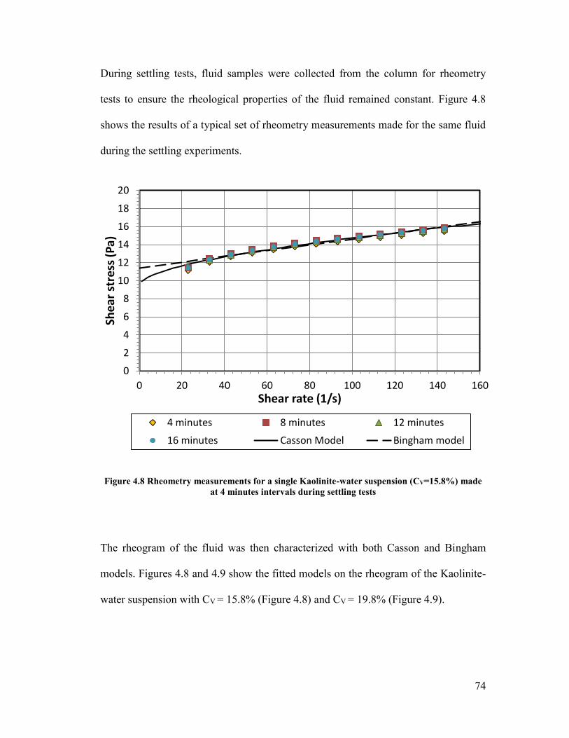
74
During settling tests, fluid samples were collected from the column for rheometry
tests to ensure the rheological properties of the fluid remained constant. Figure 4.8
shows the results of a typical set of rheometry measurements made for the same fluid
during the settling experiments.
Figure 4.8 Rheometry measurements for a single Kaolinite-water suspension (CV=15.8%) made
at 4 minutes intervals during settling tests
The rheogram of the fluid was then characterized with both Casson and Bingham
models. Figures 4.8 and 4.9 show the fitted models on the rheogram of the Kaolinite-
water suspension with CV = 15.8% (Figure 4.8) and CV = 19.8% (Figure 4.9).
0
2
4
6
8
10
12
14
16
18
20
0 20 40 60 80 100 120 140 160
She
ar s
tre
ss (
Pa)
Shear rate (1/s)
4 minutes 8 minutes 12 minutes
16 minutes Casson Model Bingham model
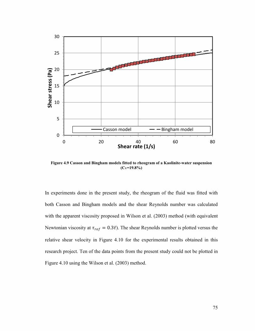
75
Figure 4.9 Casson and Bingham models fitted to rheogram of a Kaolinite-water suspension
(CV=19.8%)
In experiments done in the present study, the rheogram of the fluid was fitted with
both Casson and Bingham models and the shear Reynolds number was calculated
with the apparent viscosity proposed in Wilson et al. (2003) method (with equivalent
Newtonian viscosity at 𝜏𝑟𝑒𝑓 = 0.3𝜏). The shear Reynolds number is plotted versus the
relative shear velocity in Figure 4.10 for the experimental results obtained in this
research project. Ten of the data points from the present study could not be plotted in
Figure 4.10 using the Wilson et al. (2003) method.
0
5
10
15
20
25
30
0 20 40 60 80
She
ar s
tre
ss (
Pa)
Shear rate (1/s)
Casson model Bingham model
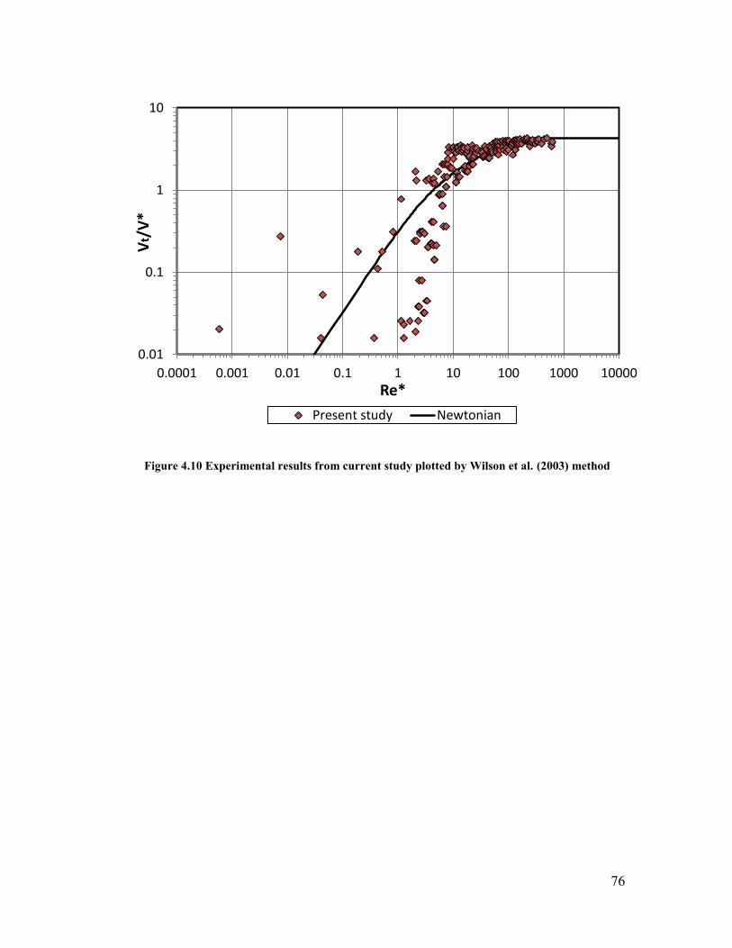
76
Figure 4.10 Experimental results from current study plotted by Wilson et al. (2003) method
0.01
0.1
1
10
0.0001 0.001 0.01 0.1 1 10 100 1000 10000
Vt/
V*
Re*
Present study Newtonian
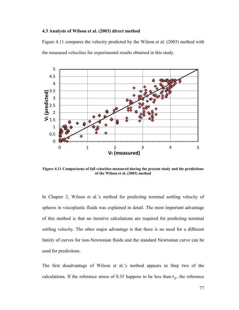
77
4.3 Analysis of Wilson et al. (2003) direct method
Figure 4.11 compares the velocity predicted by the Wilson et al. (2003) method with
the measured velocities for experimental results obtained in this study.
Figure 4.11 Comparisons of fall velocities measured during the present study and the predictions
of the Wilson et al. (2003) method
In Chapter 2, Wilson et al.’s method for predicting terminal settling velocity of
spheres in viscoplastic fluids was explained in detail. The most important advantage
of this method is that no iterative calculations are required for predicting terminal
settling velocity. The other major advantage is that there is no need for a different
family of curves for non-Newtonian fluids and the standard Newtonian curve can be
used for predictions.
The first disadvantage of Wilson et al.’s method appears in Step two of the
calculations. If the reference stress of 0.3𝜏 happens to be less than 𝜏𝑦, the reference
0
0.5
1
1.5
2
2.5
3
3.5
4
4.5
5
0 1 2 3 4 5
Vt
(pre
dic
ted
)
Vt (measured)
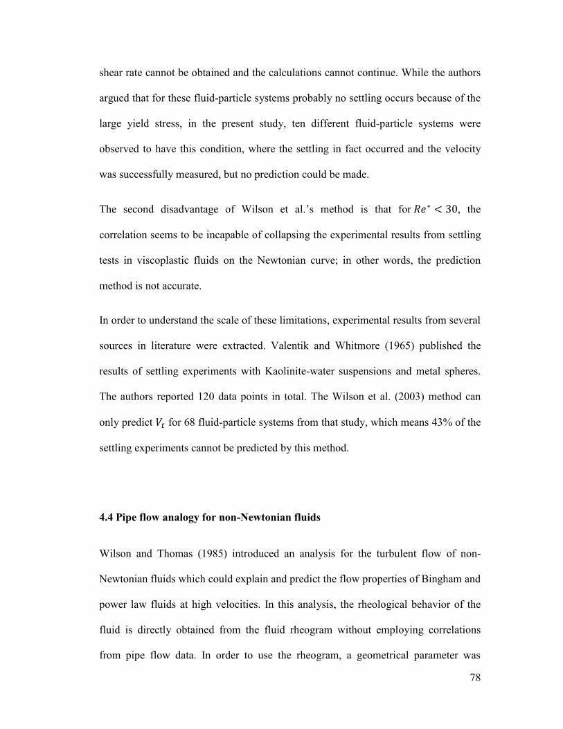
78
shear rate cannot be obtained and the calculations cannot continue. While the authors
argued that for these fluid-particle systems probably no settling occurs because of the
large yield stress, in the present study, ten different fluid-particle systems were
observed to have this condition, where the settling in fact occurred and the velocity
was successfully measured, but no prediction could be made.
The second disadvantage of Wilson et al.’s method is that for 𝑅𝑒∗ < 30, the
correlation seems to be incapable of collapsing the experimental results from settling
tests in viscoplastic fluids on the Newtonian curve; in other words, the prediction
method is not accurate.
In order to understand the scale of these limitations, experimental results from several
sources in literature were extracted. Valentik and Whitmore (1965) published the
results of settling experiments with Kaolinite-water suspensions and metal spheres.
The authors reported 120 data points in total. The Wilson et al. (2003) method can
only predict 𝑉𝑡 for 68 fluid-particle systems from that study, which means 43% of the
settling experiments cannot be predicted by this method.
4.4 Pipe flow analogy for non-Newtonian fluids
Wilson and Thomas (1985) introduced an analysis for the turbulent flow of non-
Newtonian fluids which could explain and predict the flow properties of Bingham and
power law fluids at high velocities. In this analysis, the rheological behavior of the
fluid is directly obtained from the fluid rheogram without employing correlations
from pipe flow data. In order to use the rheogram, a geometrical parameter was
79
introduced which was independent of fluid rheology model and yet could represent
fluid rheology in a specific situation. The rheogram shape factor or 𝛼 was defined as
the ratio of the area below the rheogram (from zero to a reference point), to the area
under the line for an equivalent Newtonian fluid at that reference point. Figure 4.12
shows the schematic definition of this parameter. An 𝛼 of value 1 represents a
Newtonian fluid while 𝛼 = 2 represents a pure plastic solid.
Figure 4.12 The rheogram shape factor (𝛼)
Introducing 𝛼 as the representative of fluid rheology in specific applications allowed
the researchers to model complicated processes without limiting the fluid properties
to any specific two-parameter or three-parameter rheology models.
80
In pipe flow (laminar or turbulent) the shear stress varies linearly from zero at the axis
to a maximum value at the pipe wall. The Wilson-Thomas model introduces the flow
properties as a function of 𝛼 for non-Newtonian fluids without yield stress:
𝑈
𝑈∗= 𝑓(𝜇𝑒𝑞 , 𝛼) (4.1)
where �� is the time-averaged velocity of the fluid and 𝜇𝑒𝑞 is the equivalent
Newtonian viscosity of the non-Newtonian fluid at the wall. For yield stress fluids on
the other hand, in addition to 𝛼, another parameter is introduced to represent deviation
from Newtonian behavior:
��
𝑈∗= 𝑓(𝜇𝑒𝑞, 𝛼, 𝜉) (4.2)
𝜉 =𝜏𝑦
𝜏𝑤 (4.3)
where �� is fluid velocity, 𝜏𝑦 is the fluid yield stress and 𝜏𝑤 is the wall shear stress.
In the problem of a settling sphere in a viscoplastic fluid, 𝛼 is a unique parameter that
is calculated based on a combination of fluid and particle properties. In order to
calculate 𝛼, a proper reference point with regard to the fluid application should be
selected. Following the pipe flow analogy, Wilson et al. (2003) chose the mean
surficial stress on falling sphere, or 𝜏 (Equation 2.12), as the initial reference point for
calculating 𝛼 in problem of settling sphere.
81
4.5 Analysis of rheogram shape factor
To determine 𝛼 in a settling problem, 𝜏 is first calculated as the reference point. The
rheology model of the fluid is then integrated from zero to 𝜏 to calculate the area
under the rheogram. The result of this integral is then divided by the area of the
triangle produced by linking zero to the reference point. Final formulas for calculating
𝛼 are shown in Equations (4.4) and (4.5) for Casson and Bingham models
respectively:
𝛼𝑐 = 𝜏𝑐 +
12 𝜇𝑐 �� +
43 (𝜏𝑐𝜇𝑐 ��)0.5
12 𝜏
(4.4)
𝛼𝐵 = 1 +𝜏𝐵
𝜏 (4.5)
where �� is the corresponding shear rate at the reference point. Figure 4.13 shows that
𝛼𝐶 is between 7.5% to 11.5% different from 𝛼𝐵 for the 108 data points of the present
study.
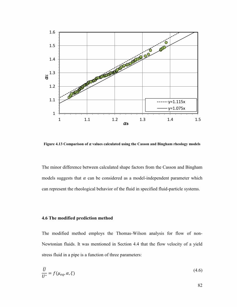
82
Figure 4.13 Comparison of 𝛼 values calculated using the Casson and Bingham rheology models
The minor difference between calculated shape factors from the Casson and Bingham
models suggests that 𝛼 can be considered as a model-independent parameter which
can represent the rheological behavior of the fluid in specified fluid-particle systems.
4.6 The modified prediction method
The modified method employs the Thomas-Wilson analysis for flow of non-
Newtonian fluids. It was mentioned in Section 4.4 that the flow velocity of a yield
stress fluid in a pipe is a function of three parameters:
��
𝑈∗= 𝑓(𝜇𝑒𝑞, 𝛼, 𝜉)
(4.6)
1
1.1
1.2
1.3
1.4
1.5
1.6
1 1.1 1.2 1.3 1.4 1.5
𝛼C
𝛼B
y=1.115x
y=1.075x
83
The objective of the modified approach developed here is to apply the pipe flow
analogy to particle settling and then find a function based on the same parameters to
relate terminal settling velocity of a sphere in a viscoplastic fluid to the properties of
the fluid-particle system. In order to do this, it is convenient to define the apparent
viscosity of the viscoplastic fluid as a function of the specified parameters. The mean
surficial stress (𝜏) is chosen as both the reference point for calculating 𝛼 and as the
characteristic shear stress used to calculate 𝜉. Experimental results published by
Valentik and Whitmore (1965), Ansley and Smith (1967), Tran et al. (1993) and
Wilson et al. (2003) were added to the experimental results from this study to increase
the number of data points and broaden the range of applicability of the modified
method.
4.7 Modification development
The proposed form of the relation between apparent viscosity and the three
parameters mentioned above is:
𝜇𝑎𝑝𝑝 = 𝜇𝑒𝑞 . 𝑓(𝛼, 𝜉) (4.7)
The general methodology is to calculate 𝜇𝑎𝑝𝑝 based on different forms of 𝑓, and
determine the errors of predicted fall velocities. The best function will be the one
which produces the smallest errors in final predictions of 𝑉𝑡. The surface-fitting
toolbox from MATLAB (r2010a) was applied using a trust-region fitting algorithm to
fit a two-variable model (based on 𝛼 and 𝜉) to define the apparent viscosity of the
viscoplastic fluids. The root mean square error (RMSE) and coefficient of
84
determination (𝑅2) for calculated and predicted velocities are the basic criteria used
to evaluate and compare different models:
𝑅𝑀𝑆𝐸 = (∑ (𝑉𝑡𝑝 − 𝑉𝑡𝑚)
2𝑛1
𝑛)0.5 (4.8)
𝑆𝑆𝑟𝑒𝑠 = ∑(𝑉𝑡𝑝 − 𝑉𝑡𝑚)2
𝑛
1
(4.9)
𝑆𝑆𝑡𝑜𝑡 = ∑(𝑉𝑡𝑚 − ��𝑡𝑚)2
𝑛
1
(4.10)
𝑅2 = 1 −𝑆𝑆𝑟𝑒𝑠
𝑆𝑆𝑡𝑜𝑡 (4.11)
where 𝑉𝑡𝑝 is the predicted terminal settling velocity, 𝑉𝑡𝑚 is the measured terminal
settling velocity, ��𝑡𝑚 is the average of measured velocities, and n is the number of
data points. The RMSE represents the sample standard deviation of the differences
between predicted values and observed values, and 𝑅2 indicates how well data fit the
statistical model (Morrison 2009).
To develop the model, an equivalent Newtonian fluid-particle system was assigned to
each measured velocity. Each 𝑉𝑡𝑚 was inserted into Newtonian relations for the
falling sphere (see Chapter 2) and a shear Reynolds number (𝑅𝑒∗𝑁
) was found by
back-calculation. The equivalent Newtonian viscosity calculated from this shear
Reynolds number is denoted by 𝜇𝑁. In order to define the apparent viscosity of the
85
viscoplastic fluid in a way that the settling data coincide with the standard Newtonian
curve, 𝜇𝑁 is assumed to be the apparent viscosity of the fluid:
𝜇𝑁 = 𝜇𝑒𝑞 . 𝑓(𝛼, 𝜉) (4.12)
and
𝜇𝑁
𝜇𝑒𝑞= 𝑓(𝛼, 𝜉)=𝛽 (4.13)
The fraction 𝜇𝑁
𝜇𝑒𝑞 has been denoted as 𝛽 for simplification. In order to discover the
optimum form of the function 𝑓, the sensitivity of 𝜇𝑁
𝜇𝑒𝑞 to 𝛼 and 𝜉 is visualized in
Figures 4.14 and 4.15. Comparison of these two graphs suggests that although no
specific pattern is visible between 𝛽 and 𝜉, the behavior of 𝛽 clearly changes when 𝛼
values become larger than 1.3. Based on these observations, the data points were
divided into two categories based on values of 𝛼.
86
Figure 4.14 The change in modeling parameter (𝛽) with increase of characteristic shear stress (𝜉)
Figure 4.15 The change in modeling parameter (𝛽) with increase of rheogram shape factor (𝜶)
0
50
100
150
200
250
300
0 0.1 0.2 0.3 0.4 0.5
b
x
0
50
100
150
200
250
300
1 1.1 1.2 1.3 1.4 1.5
b
a
87
4.7.1 Category I: fall velocity prediction for systems with 𝜶 < 𝟏. 𝟑
Surface fitting tools from MatLab (R2010a) were applied using a trust-region fitting
algorithm to fit a two-variable model (based on 𝛼 and 𝜉) to find the optimum form of
the function 𝑓(𝛼, 𝜉). A simple power form has been chosen to fit the data. Figure 4.16
visualizes the mathematical form of 𝑓. The coefficients of this equation were
optimized using a genetic algorithm. The details of the optimization method and the
codes are available in Appendices 4 and 5.
Figure 4.16 Experimental results and the fitted surface of function f, 𝛼<1.3
88
The optimization process results in Equation (4.14)
𝑓(𝛼, 𝜉) = 4.586𝛼12.878𝜉1.612 (4.14)
Table 4.3 compares the performance of the modified model with predictions by
Wilson et al.’s correlation for 252 data points with 𝛼 < 1.3.
Table 4.3 Comparison of the performance of the modified method and Wilson et al. (2003)
method for a sphere settling in a viscoplastic fluid, 𝛼<1.3
Prediction method RMSE R2
Wilson et al.’s method 0.69 0.67
Modified method 0.47 0.85
Figure 4.17 shows the comparison between the measured velocities and predicted
velocities by the modified method.
89
Figure 4.17Comparison of experimental results and predicted velocities by modified method,
𝛼<1.3
4.7.2 Category II: fall velocity prediction for systems with 𝜶 ≥ 𝟏. 𝟑
For data points with higher values of 𝛼, a different equation was found to result in
more accurate predictions. The proper form of the function was discovered by surface
fitting tools and the coefficients were optimized using genetic algorithm optimization
method. Figure 4.18 shows the three dimensional graph of the fitted equation.
0
0.5
1
1.5
2
2.5
3
0 0.5 1 1.5 2 2.5 3
Pre
dic
ted
ve
loci
ty (
m/s
)
Measured velocity (m/s)
y=x
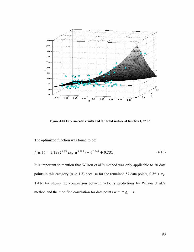
90
Figure 4.18 Experimental results and the fitted surface of function f, 𝛼≥1.3
The optimized function was found to be:
𝑓(𝛼, 𝜉) = 5.139𝜉1.55 exp(𝛼3.995) + 𝜉2.747 + 0.731 (4.15)
It is important to mention that Wilson et al.’s method was only applicable to 50 data
points in this category (𝛼 ≥ 1.3) because for the remained 57 data points, 0.3𝜏 < 𝜏𝑦.
Table 4.4 shows the comparison between velocity predictions by Wilson et al.’s
method and the modified correlation for data points with 𝛼 ≥ 1.3.
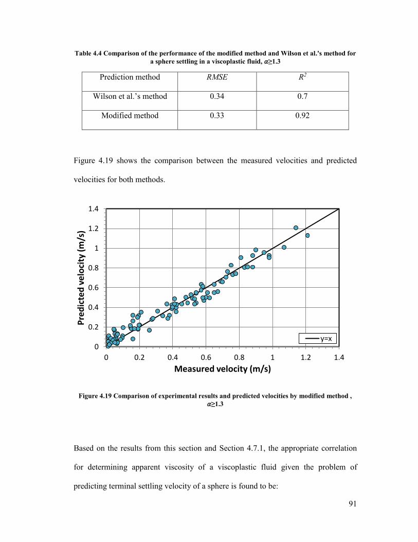
91
Table 4.4 Comparison of the performance of the modified method and Wilson et al.'s method for
a sphere settling in a viscoplastic fluid, 𝛼≥1.3
Prediction method RMSE R2
Wilson et al.’s method 0.34 0.7
Modified method 0.33 0.92
Figure 4.19 shows the comparison between the measured velocities and predicted
velocities for both methods.
Figure 4.19 Comparison of experimental results and predicted velocities by modified method ,
𝛼≥1.3
Based on the results from this section and Section 4.7.1, the appropriate correlation
for determining apparent viscosity of a viscoplastic fluid given the problem of
predicting terminal settling velocity of a sphere is found to be:
0
0.2
0.4
0.6
0.8
1
1.2
1.4
0 0.2 0.4 0.6 0.8 1 1.2 1.4
Pre
dic
ted
ve
loci
ty (
m/s
)
Measured velocity (m/s)
y=x
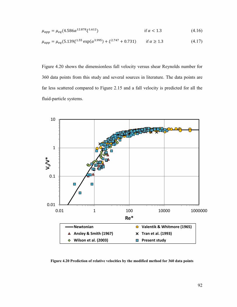
92
𝜇𝑎𝑝𝑝 = 𝜇𝑒𝑞(4.586𝛼12.878𝜉1.612) if 𝛼 < 1.3 (4.16)
𝜇𝑎𝑝𝑝 = 𝜇𝑒𝑞(5.139𝜉1.55 exp(𝛼3.995) + 𝜉2.747 + 0.731) if 𝛼 ≥ 1.3 (4.17)
Figure 4.20 shows the dimensionless fall velocity versus shear Reynolds number for
360 data points from this study and several sources in literature. The data points are
far less scattered compared to Figure 2.15 and a fall velocity is predicted for all the
fluid-particle systems.
Figure 4.20 Prediction of relative velocities by the modified method for 360 data points
0.01
0.1
1
10
0.01 1 100 10000 1000000
Vt/
V*
Re*
Newtonian Valentik & Whitmore (1965)
Ansley & Smith (1967) Tran et al. (1993)
Wilson et al. (2003) Present study
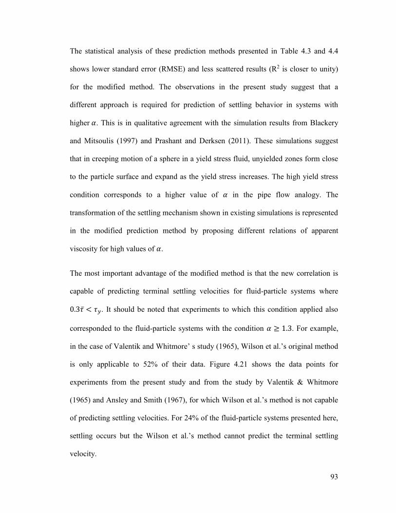
93
The statistical analysis of these prediction methods presented in Table 4.3 and 4.4
shows lower standard error (RMSE) and less scattered results (R2 is closer to unity)
for the modified method. The observations in the present study suggest that a
different approach is required for prediction of settling behavior in systems with
higher 𝛼. This is in qualitative agreement with the simulation results from Blackery
and Mitsoulis (1997) and Prashant and Derksen (2011). These simulations suggest
that in creeping motion of a sphere in a yield stress fluid, unyielded zones form close
to the particle surface and expand as the yield stress increases. The high yield stress
condition corresponds to a higher value of 𝛼 in the pipe flow analogy. The
transformation of the settling mechanism shown in existing simulations is represented
in the modified prediction method by proposing different relations of apparent
viscosity for high values of 𝛼.
The most important advantage of the modified method is that the new correlation is
capable of predicting terminal settling velocities for fluid-particle systems where
0.3𝜏 < 𝜏𝑦. It should be noted that experiments to which this condition applied also
corresponded to the fluid-particle systems with the condition 𝛼 ≥ 1.3. For example,
in the case of Valentik and Whitmore’ s study (1965), Wilson et al.’s original method
is only applicable to 52% of their data. Figure 4.21 shows the data points for
experiments from the present study and from the study by Valentik & Whitmore
(1965) and Ansley and Smith (1967), for which Wilson et al.’s method is not capable
of predicting settling velocities. For 24% of the fluid-particle systems presented here,
settling occurs but the Wilson et al.’s method cannot predict the terminal settling
velocity.
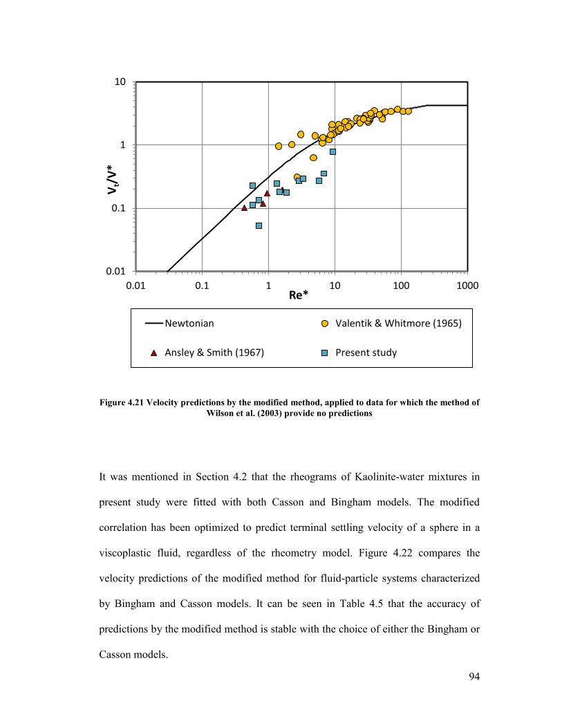
94
Figure 4.21 Velocity predictions by the modified method, applied to data for which the method of
Wilson et al. (2003) provide no predictions
It was mentioned in Section 4.2 that the rheograms of Kaolinite-water mixtures in
present study were fitted with both Casson and Bingham models. The modified
correlation has been optimized to predict terminal settling velocity of a sphere in a
viscoplastic fluid, regardless of the rheometry model. Figure 4.22 compares the
velocity predictions of the modified method for fluid-particle systems characterized
by Bingham and Casson models. It can be seen in Table 4.5 that the accuracy of
predictions by the modified method is stable with the choice of either the Bingham or
Casson models.
0.01
0.1
1
10
0.01 0.1 1 10 100 1000
Vt/
V*
Re*
Newtonian Valentik & Whitmore (1965)
Ansley & Smith (1967) Present study
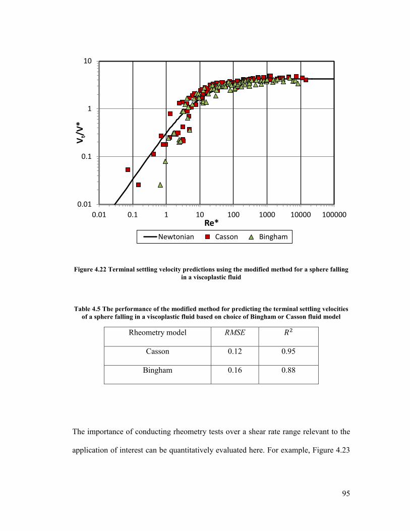
95
Figure 4.22 Terminal settling velocity predictions using the modified method for a sphere falling
in a viscoplastic fluid
Table 4.5 The performance of the modified method for predicting the terminal settling velocities
of a sphere falling in a viscoplastic fluid based on choice of Bingham or Casson fluid model
Rheometry model RMSE 𝑅2
Casson 0.12 0.95
Bingham 0.16 0.88
The importance of conducting rheometry tests over a shear rate range relevant to the
application of interest can be quantitatively evaluated here. For example, Figure 4.23
0.01
0.1
1
10
0.01 0.1 1 10 100 1000 10000 100000
Vt/
V*
Re*
Newtonian Casson Bingham
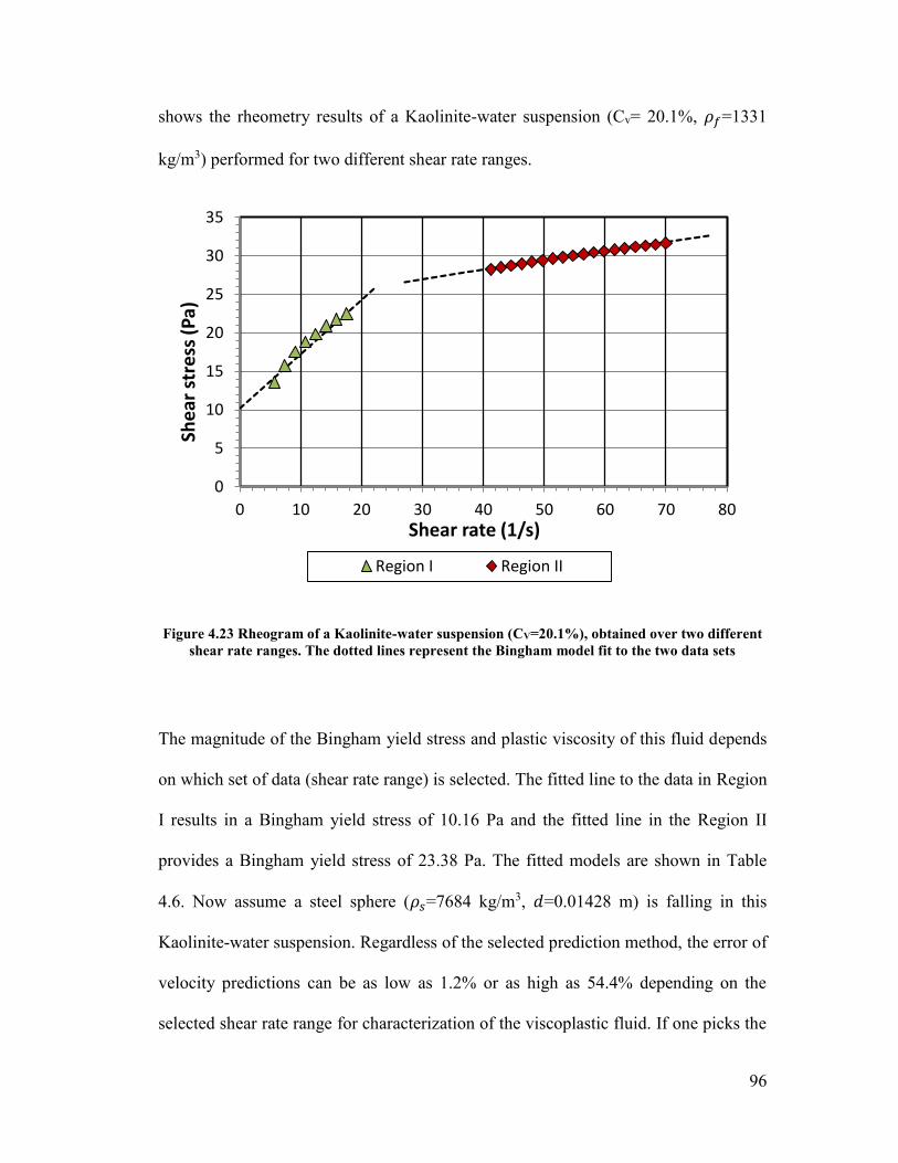
96
shows the rheometry results of a Kaolinite-water suspension (Cv= 20.1%, 𝜌𝑓=1331
kg/m3) performed for two different shear rate ranges.
Figure 4.23 Rheogram of a Kaolinite-water suspension (CV=20.1%), obtained over two different
shear rate ranges. The dotted lines represent the Bingham model fit to the two data sets
The magnitude of the Bingham yield stress and plastic viscosity of this fluid depends
on which set of data (shear rate range) is selected. The fitted line to the data in Region
I results in a Bingham yield stress of 10.16 Pa and the fitted line in the Region II
provides a Bingham yield stress of 23.38 Pa. The fitted models are shown in Table
4.6. Now assume a steel sphere (𝜌𝑠=7684 kg/m3, 𝑑=0.01428 m) is falling in this
Kaolinite-water suspension. Regardless of the selected prediction method, the error of
velocity predictions can be as low as 1.2% or as high as 54.4% depending on the
selected shear rate range for characterization of the viscoplastic fluid. If one picks the
0
5
10
15
20
25
30
35
0 10 20 30 40 50 60 70 80
She
ar s
tre
ss (
Pa)
Shear rate (1/s)
Region I Region II
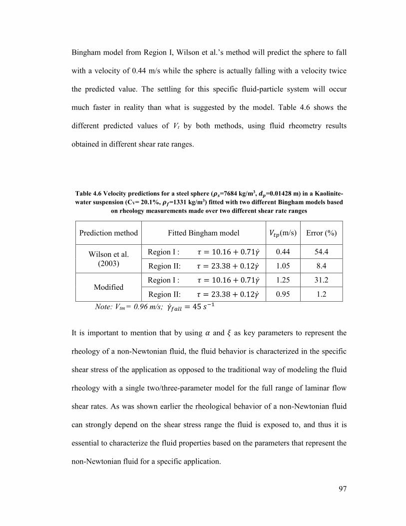
97
Bingham model from Region I, Wilson et al.’s method will predict the sphere to fall
with a velocity of 0.44 m/s while the sphere is actually falling with a velocity twice
the predicted value. The settling for this specific fluid-particle system will occur
much faster in reality than what is suggested by the model. Table 4.6 shows the
different predicted values of Vt by both methods, using fluid rheometry results
obtained in different shear rate ranges.
Table 4.6 Velocity predictions for a steel sphere (𝝆𝒔=7684 kg/m3, 𝒅𝒑=0.01428 m) in a Kaolinite-
water suspension (CV= 20.1%, 𝝆𝒇=1331 kg/m3) fitted with two different Bingham models based
on rheology measurements made over two different shear rate ranges
Prediction method Fitted Bingham model 𝑉𝑡𝑝(m/s) Error (%)
Wilson et al.
(2003)
Region I : 𝜏 = 10.16 + 0.71�� 0.44 54.4
Region II: 𝜏 = 23.38 + 0.12�� 1.05 8.4
Modified Region I : 𝜏 = 10.16 + 0.71�� 1.25 31.2
Region II: 𝜏 = 23.38 + 0.12�� 0.95 1.2
Note: Vtm = 0.96 m/s; ��𝑓𝑎𝑙𝑙 = 45 𝑠−1
It is important to mention that by using 𝛼 and 𝜉 as key parameters to represent the
rheology of a non-Newtonian fluid, the fluid behavior is characterized in the specific
shear stress of the application as opposed to the traditional way of modeling the fluid
rheology with a single two/three-parameter model for the full range of laminar flow
shear rates. As was shown earlier the rheological behavior of a non-Newtonian fluid
can strongly depend on the shear stress range the fluid is exposed to, and thus it is
essential to characterize the fluid properties based on the parameters that represent the
non-Newtonian fluid for a specific application.
98
5. Conclusions and recommendations for future work
5.1 Summary and conclusions
The primary objective of this research was to conduct high-quality measurements of
the terminal settling velocities of single spheres falling in viscoplastic fluids, with a
focus on the collection of data under conditions where existing correlations provide
poor (or no) predictions. The new data, in combination with data taken from the
literature, were then used to form the basis for a new, improved settling velocity
correlation.
The following points summarize the key findings of the present study:
A quantitative analysis of the Wilson et al. method (2003) for predicting
terminal settling velocity of spheres in viscoplastic fluids was conducted. This
method provides good predictions for cases where Re* > 100. In this region,
the average absolute error is 9.7% for 133 data points taken from the
literature. For conditions where Re* < 100, the average absolute error is 75%
for 62 experimental points.
The limitations of the Wilson et al. method (2003) were recognized and
analyzed based on the available data in the literature, specifically, this method
is (a) not applicable for systems with 0.3𝜏 < 𝜏𝑦 , and (b) does not produce
accurate predictions for systems with 𝑅𝑒∗<100.
An experimental methodology was developed for measuring terminal settling
velocity of spheres in Kaolinite-water suspensions using Electrical Impedance
Tomography (EIT).
99
More than 30 Kaolinite-water mixtures with concentrations ranging from
10.6% to 21.7% by volume were prepared and used as the viscoplastic
medium for settling tests. Precision spheres with different sizes and densities
were used for settling tests.
Rheometry tests were carefully conducted over the shear rate ranges
experienced by the fluid surrounding the particle. Both Casson and Bingham
models were used to model the rheogram of the fluid.
The analogy of Wilson-Thomas model for the turbulent pipe flow of non-
Newtonian fluids was followed to study the fall velocity of spheres in
viscoplastic fluids. The rheogram shape factor (𝛼) and relative shear stress (𝜉)
were recognized as key parameters for yield stress fluids. The apparent
viscosity of the viscoplastic fluid was defined based on these two parameters.
The modified correlation covers the systems with 0.3𝜏 < 𝜏𝑦 and produces
more accurate predictions for low 𝑅𝑒∗ regions. The accuracy of predictions
obtained with the modified method is higher than previous prediction methods
and the standard error is stable regardless of whether the Bingham or Casson
model is used for characterization of the viscoplastic fluid.
The analysis presented here also emphasizes the importance of making
rheology measurements at relevant shear rates in order to accurately predict
terminal settling velocities for particles in viscoplastic fluids.
100
5.2 Recommendations for future work
The method proposed in this research has been developed based on
calculations of 𝛼 using Casson and Bingham models. Experimental results
using Herschel-Bulkley fluids should be obtained and an analysis of the
sensitivity of the modified method to the rheogram shape factor should be
completed
Spheres with rough surfaces should be tested with the same methodology to
analyze the effects of surface roughness on the fall velocity of particles.
Spherical particles are idealized form of the real irregular shaped particles
present in industrial applications. Although prediction methods like this can
produce an estimation of fall velocity for particles in real situations, more
experimental work should be done to study the settling characteristics of non-
spherical particles in non-Newtonian fluids.
Since the size and shape of the sheared zone around a non-spherical particle
falling in a viscoplastic medium are more complicated because of several
factors such as to non-symmetric drag force, particle rotation and orientation,
it is essential to conduct settling experiments in different conditions where
three dimensional information describing the position of the particle at any
moment during the fall is collected.
101
References
Andres, U. Ts. "Equilibrium and motion of spheres in a viscoplastic liquid." Soviet
Physics Doklady. (U.S.A), 5 ,p723 (1961).
Ansley, R.W., Smith, T.N., “Motion of Spherical Particles in a Bingham Plastic”,
AIChE. Journal, 13, p1193 (1967).
AR-G2/AR2000ex/AR 1500ex Manual. January (2011).
Atapattu, D. D. Ph.D. dissertation. Melbourne: Monash University, (1989).
Atapattu, D.D., Chhabra, R. P., Uhlherr, P.H.T. "Creeping sphere motion in
Herschel-Bulkley fluids: flow field and drag." Journal of non-Newtonian Fluid
Mechanics, 59, p245 (1995).
Atapattu, D.D., Chhabra, R.P., Tiu, C., Uhlherr, P.H.T. "The effect of cylindrical
boundaries for spheres falling in fluids having a yield stress." Australasian Fluid
Mech. Conf., Auckland,p584 (1986).
Atapattu, D.D., Chhabra, R.P., Uhlherr, P. H. T. "Wall effect for spheres falling at
small Reynolds number in a viscoplastic medium." Journal of non-Newtonian Fluid
Mechanics 38, p31 (1990).
Barnes, H. A., Walters, K. "The yield stress myth?" Rheological Acta 24, p323
(1985).
Beaulne, M., Mitsoulis, E. "Creeping motion of a sphere in tubes filled with Herschel-
Bulkley fluids", Journal of non-Newtonian fluid Mechanics, 72, p55 (1997).
Beris, A. N., Tsamopoulos, J., Armstrong, R. C., Brown, R. A. "Creeping motion of a
sphere through a Bingham plastic" Journal of Fluid Mechanics 158, p219 (1985).
Bird, R.B., Stewart, W.E., Lightfoot, E.N. Transport Phenomena. New York: J.
Willey, (2007).
Blackery, J., Mitsoulis, E. "Creeping motion of a sphere in tubes filled with a
Bingham plastic material", Journal of non-Newtonian Fluid Mechanincs, 70, p59
(1997).
Boardman, G. Whitmore, R.L. "The static measurement of yield stress" Laboratory
Practice 10, p782 (1961).
102
Brown, B.H. "Electerical Impedence Tomography (EIT)-A reveiw." J. Med. Eng.
Technol. 27(3), p97 (2003).
Carreau, P.J., Dekee, D., Chhabra, R.P. Rheology of polymeric systems. Munich:
Hanser, (1997).
Chafe, N. P., de Bruyn, J. R. "Drag and relaxation in a bentonite clay suspension."
Journal of non-Newtonian Fluid Mechanics 131, p44 (2005).
Chhabra, R. P, Agrawal, S., Chaudhary, K. "A note on wall effect on the terminal
falling velocity of a sphere in quiescent Newtonian media in cylindrical tubes."
Powder Technology 129, p53 (2003).
Chhabra, R.P. Bubbles, drops, and particles in non-Newtonian fluids. Taylor &
Francis, (2007).
Clift, R., Grace, J.R., Weber, M. E. Bubbles, drops, and particles. New York:
Academic Press (1978).
Colebrook, C. F. "Turbulent flow in pipes, with particular reference to transition
region between the smooth and rough pipe laws." Journal of the Institute of Civil
Engineers 11, p133 (1938).
Cooke, R. "Laminar flow settling: the potential for unexpected problems", Proc.
Hydrotransport 15. Banff, AB, Canada: BHR Group, Cranfield, UK, p121 (2002).
Di Felice, R. "A relationsship for the wall effect on the settling velocity of a sphere at
any flow regime" International Journal of Multiphase Flow,22, p527 (1996).
du Plessis, M. P., Ansley, R. W. "Settling parameters in solids pipelining" J.Pipeline
Div. (ASCE), 93, (1967).
Elliot, D. E., Gilddon, B. J. "Hydraulic transport of coal at high concentrations."
Hydrotransport 1. Cranfield, UK: BHRA, paper G2 (1970).
Gillies, R. G., Hill, K.B., McKibben, M. J., Shook, C. A. "A method for estimating
deposition velocities for pseudohomogeneous slurries." Proc. ASME Eng Div.
Summer Meeting. Vancouver, BC, Canada, (1997).
Gillies, R. G., Shook, C. A. "Concentration Distributions of Sand Slurries in
Horizontal Pipe Flow", Particle Science Technology, 12, p45 (1994).
Gillies, R. G., Sun, R., Sanders, R. S., Schaan, J. "Lowered expctations: The impact of
yield stress on sand transport in laminar, non-Newtonian slurry flows." Journal of the
Southern African Institute of Mining and Metallurgy, vol 107, p351 (2007).
103
Gillies. R. G., Hill, K. B., McKibben, M. J., Shook, C.A. "Solids transport by laminar
Newtonian flows." Powder Technology 104, p269 (1999).
Graham. L., Hamilton, R., Rudman, M., Strode, P., Pullum. L. "Coarse solid
concentration profiles in laminar pipe flo." Hydrotransport 15. Banff, Canada: BHR
Group., (2003).
Gumulya, M. The settling of spheres in viscoplastic fluids. PhD Thesis, Perth,
Australia: Curtain University of Technology, (2009).
Haberman, W.L., Sayre, R. M. David Taylor Model Basin. Washington: U.S. Navy
Department, (1958).
Hariharaputhiran, M., Shankar Subramanian, R., Campbell, G. A., Chhabra, R.P.
"The settling of spheres in a viscoplastic medium." Journal of non-Newtonian FLuid
Mechanics, 79, p87 (1998).
Hashemi, S. A. "Velocity and concentration fluctuations in concentrated solid-liquid
flows." PhD dissertation. Edmonton: University of Alberta, (2013).
Kaushal, D. R., Tomita, Y. "Prediction of Concentration Distribution in Pipeline
Flow of Highly Concentrated Slurry." Particle Science Technology, 31, p28(2013).
L., Pullum. Pipeline performance. Melbourne, Australia: Paste 2003, (2003).
Litzenberger, C. G., Sumner, R. J. "Flow behavior of Kaolin clay slurries."
Hydrotransport 16. Cranfield, U.K.: BHR Group, p77 (2004).
Masliyah, J., Czanecki, J., Xu, Z. Handbook on theory and practice of bitumen
recovery from Athabasca oil sands, Volume 1: Theoretical basis. Kingsley Publishing
Services, (2011).
Michaels, A.S., Bolger, J.C. "The plastic flow behavior of flocculated Kaolin
suspensions." Industrial and Engineering Chemistry Fundamentals 1, no. 3, p153
(1962).
Morrison, S. J. Introduction to Engineering Statistics. Chichester, West Sussex, UK:
Hoboken, NJ: Wiley, (2009).
Nasser, M. S., James, A. E. "Settling and sediment bed behavior of kaolinite in
aqueous media." Separation and Purifiacation Technology 51, p10 (2006).
Newton, I. Principia. Section I, II, III. Cambridge, London: Macmillan and Co.,
(1863).
104
Nguyen, Q. D., Boger, D. V. "Application of Rheology to Pipeline Transport,
Dewatering and Disposal of Mineral Tailings." 9th International Conference of
Transport and Sedimentation of Solid Particles. Crascow, Poland, p 177(1997).
Prandtl, L. "Neuere Ergebnisse Turbulnzforschung." Z. Ver. Deutsch. Ing 77, 5,
p105(1933).
Prashant, Derksen, J. J. "Direct simulations of spherical particle motion in Bingham
liquids." Computers and Chemical Engineeinrg, p1200 (2011).
Pullum, L., Graham, L. J. W., Slatter, P. "A non-Newtonian two-layer model and its
application to high density hydrotransport." Hydrotransport 16th. Santiago, Chile.:
BHR Group., p579 (2004).
De Felice. R., "A relationship for the wall effect on the settling velocity of a sphere at
any flow regime." International Journal of Multiphase Flow 22, p527 (1996).
Rahman, M. H. Yield stress of mixtures with bimodal size distributions. MSc Thesis,
Edmonton: University of Alberta, (2011).
Rhodes, Martin. Introduction to particle technology. West Sussex: John Wiley and
Sons. Ltd, (2008).
Saha, G., Purohit, N.K, Mitra, A.K. "Spherical particle terminal settling velocity and
drag in Bingham liquids." International Journal of Mineral Processing, 36, p273
(1992).
Schaan, J., Sanders, R. S., Gillies, R. G., McKibben, M. J., Litzenberger, C., Sun, R.
J., Shook, C. A. "Effects of shear history on flow properties of flocculant-dosed
thickened tailings slurries." Hydrotransport 16. Cranfield, U.K.: BHR Group,.
p403(2004).
Shook, C.A., Gillies, R. G., Sanders, R. S. Pipeline Hydrotransport with Applications
in the Oil Sands Industry. Saskatoon: Saskatchewan Research Council, (2002).
Stokes, G. G. "On the effect of internal friction of fluids on the motion of pendulums."
Transactions of the Cambridge Philosophical Society 9, p48 (1851).
Talmon, A. M., van Kesteren, G. M., Sittoni, L., Hedbolm, E.P.,. "Shear cell tests for
quantification of tailings segregation", Canadian Journal of Chemical Engineering,
p362 (2014).
Thomas, A. D., Pullum, L., Wilson, K.C. "Stabilized laminar slurry flow: review,
trends and prognosis." Hydrotransport 16. Cranefield, UK: BHR Group, p701 (2004).
105
Thomas, A.D. "Coarse Particles in a Heavy Medium- Turbulent Pressure Drop
Reduction and Deposition under Laminar Flow." Proc. 5th International Conference
of the Hydraulic Transport of Solids in Pipes. Hanover, Germany, (1978).
Tran, Q.K., Trinh, D.T., Horsley, R.R., Reizes, J.A. "Drag coefficients and settlng
velocities of spheres in yield-pseudoplastic slurries." ASME Winter Annual Meeting.
New Orleans, LA, (1993).
Uhlherr, P.H.T. "A novel method for measuring yield stress in static fluids." IVth
National Conference of Rheology. Adelaide, p231 (1986).
Valentik, L., Whitmore, R.L. "The terminal velocity of spheres in Bingham plastics."
Br. J. Appl. Phys. 16, p1197 (1965).
van Olphen, H. A Introduction to Clay Colloid Chemistry. New York: Wiley-
Interscience, (1977).
Volarovich, M. P., Gutkin, A. M. "Theory of flow of a viscoplastic medium." Colloid
Journal. USSR, 15, p153 (1953).
Whyte, F. M. Fluid Mechanics, 4th Ed. McGraw-Hill, Boston, USA, (1999).
Wilson, K. C., Addie, G. R., Sellgren, A., Clift, R. Slurry Transport Using
Centrifugal Pumps. New York: Springer (2005).
Wilson, K.C, Horsely, R.R., Kealy, T., Reizes, J. C., Horsley, M. "Direct prediction
of fall velocities in non-Newtonian materials." International Journal of Mineral
Processing 71/1-4, p17 (2003).
Wilson, K.C., Horsley, R.R. "Calculating fall velocities in non-Newtonian (and
Newtonian) fluids: a new review." Hydrotransport 16. Cranefield, UK: BHR Group,
p37(2004).
Wilson, K.C., Thomas, A. D. "A new analysis of the turbulent flow of non-Newtonian
fluids." Canadian Journal of Chemical Engineering, p539 (1985).
Yoshika, N., Adachi, K. "On variational principles for a non-Newtonian fluid." J.
Chem. Eng. Jpn, 4, p217 (1971).
"z8000 EIT product sheet." www.itoms.com .
http://pdf.directindustry.com/pdf/industrial-tomography-systems/z8000-electrical-
impedance-tomography-product-sheet/40901-51620.html (accessed Feburary 25,
2015).
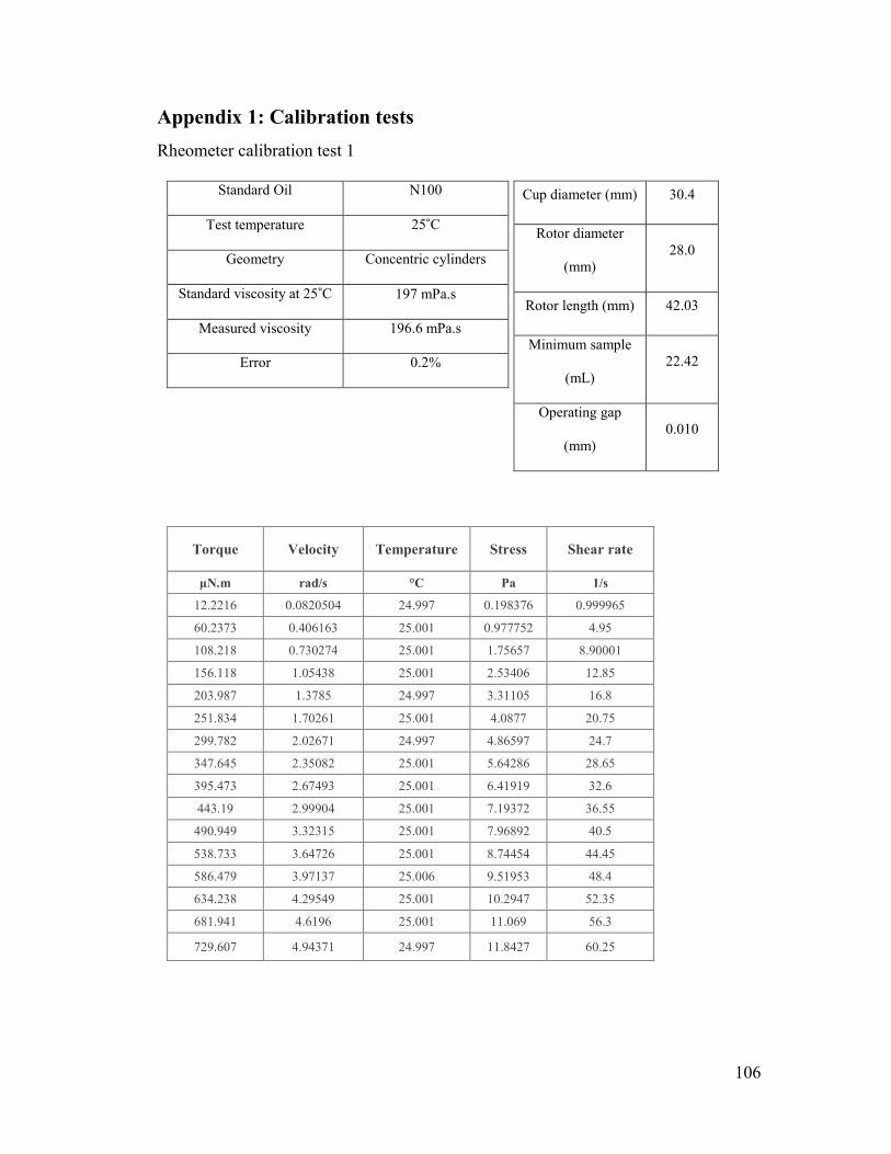
106
Appendix 1: Calibration tests
Rheometer calibration test 1
Cup diameter (mm) 30.4
Rotor diameter
(mm)
28.0
Rotor length (mm) 42.03
Minimum sample
(mL)
22.42
Operating gap
(mm)
0.010
Torque Velocity Temperature Stress Shear rate
µN.m rad/s °C Pa 1/s
12.2216 0.0820504 24.997 0.198376 0.999965
60.2373 0.406163 25.001 0.977752 4.95
108.218 0.730274 25.001 1.75657 8.90001
156.118 1.05438 25.001 2.53406 12.85
203.987 1.3785 24.997 3.31105 16.8
251.834 1.70261 25.001 4.0877 20.75
299.782 2.02671 24.997 4.86597 24.7
347.645 2.35082 25.001 5.64286 28.65
395.473 2.67493 25.001 6.41919 32.6
443.19 2.99904 25.001 7.19372 36.55
490.949 3.32315 25.001 7.96892 40.5
538.733 3.64726 25.001 8.74454 44.45
586.479 3.97137 25.006 9.51953 48.4
634.238 4.29549 25.001 10.2947 52.35
681.941 4.6196 25.001 11.069 56.3
729.607 4.94371 24.997 11.8427 60.25
Standard Oil N100
Test temperature 25˚C
Geometry Concentric cylinders
Standard viscosity at 25˚C 197 mPa.s
Measured viscosity 196.6 mPa.s
Error 0.2%
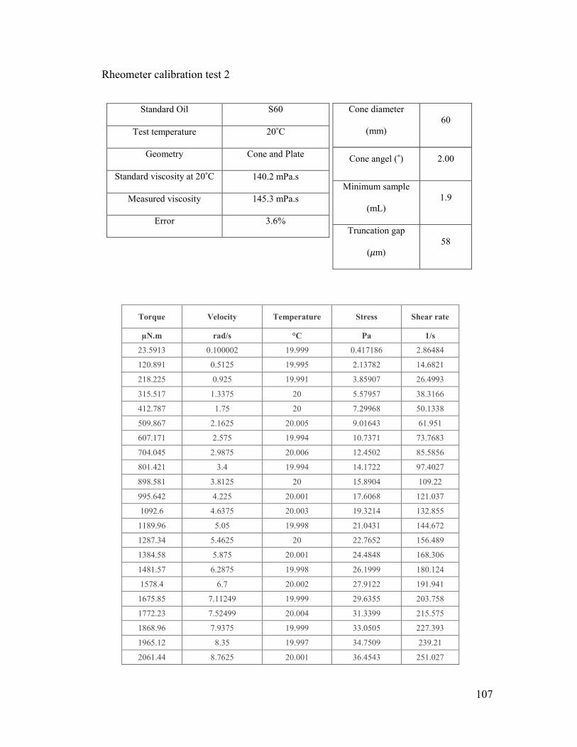
107
Rheometer calibration test 2
Cone diameter
(mm)
60
Cone angel (˚) 2.00
Minimum sample
(mL)
1.9
Truncation gap
(𝜇m)
58
Torque Velocity Temperature Stress Shear rate
µN.m rad/s °C Pa 1/s
23.5913 0.100002 19.999 0.417186 2.86484
120.891 0.5125 19.995 2.13782 14.6821
218.225 0.925 19.991 3.85907 26.4993
315.517 1.3375 20 5.57957 38.3166
412.787 1.75 20 7.29968 50.1338
509.867 2.1625 20.005 9.01643 61.951
607.171 2.575 19.994 10.7371 73.7683
704.045 2.9875 20.006 12.4502 85.5856
801.421 3.4 19.994 14.1722 97.4027
898.581 3.8125 20 15.8904 109.22
995.642 4.225 20.001 17.6068 121.037
1092.6 4.6375 20.003 19.3214 132.855
1189.96 5.05 19.998 21.0431 144.672
1287.34 5.4625 20 22.7652 156.489
1384.58 5.875 20.001 24.4848 168.306
1481.57 6.2875 19.998 26.1999 180.124
1578.4 6.7 20.002 27.9122 191.941
1675.85 7.11249 19.999 29.6355 203.758
1772.23 7.52499 20.004 31.3399 215.575
1868.96 7.9375 19.999 33.0505 227.393
1965.12 8.35 19.997 34.7509 239.21
2061.44 8.7625 20.001 36.4543 251.027
Standard Oil S60
Test temperature 20˚C
Geometry Cone and Plate
Standard viscosity at 20˚C 140.2 mPa.s
Measured viscosity 145.3 mPa.s
Error 3.6%
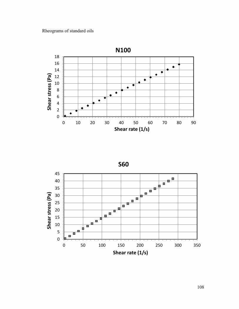
108
Rheograms of standard oils
0
2
4
6
8
10
12
14
16
18
0 10 20 30 40 50 60 70 80 90
She
ar s
tre
ss (
Pa)
Shear rate (1/s)
N100
0
5
10
15
20
25
30
35
40
45
0 50 100 150 200 250 300 350
She
ar s
tre
ss (
Pa)
Shear rate (1/s)
S60
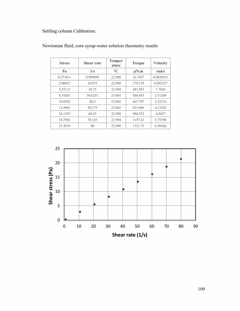
109
Settling column Calibration:
Newtonian fluid, corn syrup-water solution rheometry results
Stress Shear rate Temper
ature Torque Velocity
Pa 1/s °C µN.m rad/s
0.271811 0.999999 22.998 16.7457 0.0820531
2.90837 10.875 22.998 179.179 0.892327
5.55112 20.75 22.994 341.993 1.7026
8.19201 30.6251 23.003 504.693 2.51289
10.8393 40.5 23.003 667.787 3.32316
13.4901 50.375 23.003 831.096 4.13343
16.1397 60.25 22.998 994.332 4.9437
18.7902 70.125 22.994 1157.62 5.75398
21.4539 80 22.998 1321.73 6.56426
0
5
10
15
20
25
0 10 20 30 40 50 60 70 80 90
She
ar s
tre
ss (
Pa)
Shear rate (1/s)
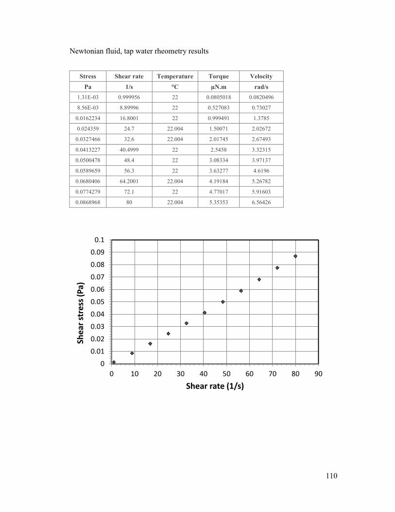
110
Newtonian fluid, tap water rheometry results
Stress Shear rate Temperature Torque Velocity
Pa 1/s °C µN.m rad/s
1.31E-03 0.999956 22 0.0805018 0.0820496
8.56E-03 8.89996 22 0.527083 0.73027
0.0162234 16.8001 22 0.999491 1.3785
0.024359 24.7 22.004 1.50071 2.02672
0.0327466 32.6 22.004 2.01745 2.67493
0.0413227 40.4999 22 2.5458 3.32315
0.0500478 48.4 22 3.08334 3.97137
0.0589659 56.3 22 3.63277 4.6196
0.0680406 64.2001 22.004 4.19184 5.26782
0.0774279 72.1 22 4.77017 5.91603
0.0868968 80 22.004 5.35353 6.56426
0
0.01
0.02
0.03
0.04
0.05
0.06
0.07
0.08
0.09
0.1
0 10 20 30 40 50 60 70 80 90
She
ar s
tre
ss (
Pa)
Shear rate (1/s)
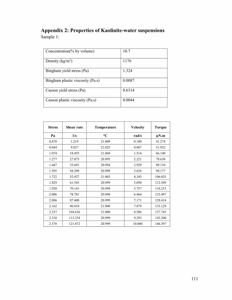
111
Appendix 2: Properties of Kaolinite-water suspensions
Sample 1:
Concentration(% by volume) 10.7
Density (kg/m3) 1176
Bingham yield stress (Pa) 1.324
Bingham plastic viscosity (Pa.s) 0.0087
Casson yield stress (Pa) 0.6314
Casson plastic viscosity (Pa.s) 0.0044
Stress Shear rate Temperature Velocity Torque
Pa 1/s °C rad/s µN.m
0.670 1.219 21.009 0.100 41.274
0.844 9.837 21.025 0.807 51.932
1.074 18.455 21.004 1.514 66.140
1.277 27.073 20.995 2.221 78.638
1.447 35.691 20.994 2.929 89.110
1.595 44.309 20.998 3.636 98.177
1.722 52.927 21.003 4.343 106.025
1.829 61.545 20.999 5.050 112.589
1.920 70.163 20.998 5.757 118.215
2.006 78.781 20.998 6.464 123.497
2.086 87.400 20.999 7.171 128.414
2.162 96.018 21.000 7.879 133.129
2.237 104.636 21.000 8.586 137.743
2.310 113.254 20.999 9.293 142.200
2.378 121.872 20.999 10.000 146.397
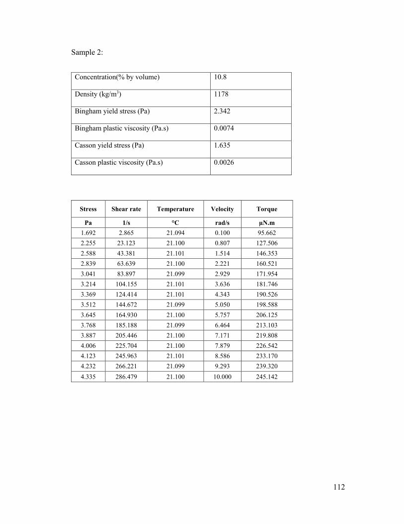
112
Sample 2:
Concentration(% by volume) 10.8
Density (kg/m3) 1178
Bingham yield stress (Pa) 2.342
Bingham plastic viscosity (Pa.s) 0.0074
Casson yield stress (Pa) 1.635
Casson plastic viscosity (Pa.s) 0.0026
Stress Shear rate Temperature Velocity Torque
Pa 1/s °C rad/s µN.m
1.692 2.865 21.094 0.100 95.662
2.255 23.123 21.100 0.807 127.506
2.588 43.381 21.101 1.514 146.353
2.839 63.639 21.100 2.221 160.521
3.041 83.897 21.099 2.929 171.954
3.214 104.155 21.101 3.636 181.746
3.369 124.414 21.101 4.343 190.526
3.512 144.672 21.099 5.050 198.588
3.645 164.930 21.100 5.757 206.125
3.768 185.188 21.099 6.464 213.103
3.887 205.446 21.100 7.171 219.808
4.006 225.704 21.100 7.879 226.542
4.123 245.963 21.101 8.586 233.170
4.232 266.221 21.099 9.293 239.320
4.335 286.479 21.100 10.000 245.142
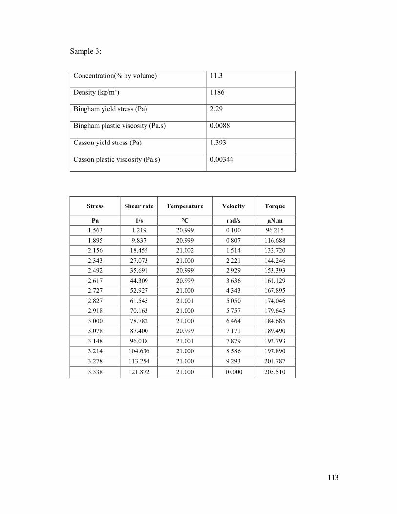
113
Sample 3:
Concentration(% by volume) 11.3
Density (kg/m3) 1186
Bingham yield stress (Pa) 2.29
Bingham plastic viscosity (Pa.s) 0.0088
Casson yield stress (Pa) 1.393
Casson plastic viscosity (Pa.s) 0.00344
Stress Shear rate Temperature Velocity Torque
Pa 1/s °C rad/s µN.m
1.563 1.219 20.999 0.100 96.215
1.895 9.837 20.999 0.807 116.688
2.156 18.455 21.002 1.514 132.720
2.343 27.073 21.000 2.221 144.246
2.492 35.691 20.999 2.929 153.393
2.617 44.309 20.999 3.636 161.129
2.727 52.927 21.000 4.343 167.895
2.827 61.545 21.001 5.050 174.046
2.918 70.163 21.000 5.757 179.645
3.000 78.782 21.000 6.464 184.685
3.078 87.400 20.999 7.171 189.490
3.148 96.018 21.001 7.879 193.793
3.214 104.636 21.000 8.586 197.890
3.278 113.254 21.000 9.293 201.787
3.338 121.872 21.000 10.000 205.510
114
Sample 4:
Concentration(% by volume) 10.6
Density (kg/m3) 1174
Bingham yield stress (Pa) 4.1
Bingham plastic viscosity (Pa.s) 0.0098
Casson yield stress (Pa) 2.96
Casson plastic viscosity (Pa.s) 0.0028
Stress Shear rate Temperature Velocity Torque
Pa 1/s °C rad/s µN.m
1.941 2.865 20.798 0.100 109.734
2.849 23.123 20.795 0.807 161.128
3.652 43.381 20.797 1.514 206.522
4.426 63.639 20.798 2.221 250.256
4.875 83.897 20.802 2.929 275.664
5.174 104.155 20.797 3.636 292.566
5.418 124.413 20.805 4.343 306.407
5.630 144.672 20.798 5.050 318.377
5.827 164.930 20.800 5.757 329.534
6.006 185.188 20.799 6.464 339.639
6.169 205.446 20.800 7.171 348.858
6.324 225.704 20.803 7.879 357.591
6.478 245.963 20.797 8.586 366.323
6.627 266.221 20.800 9.293 374.751
6.750 286.479 20.800 10.000 381.728
115
Sample 5:
Concentration(% by volume) 11.1
Density (kg/m3) 1182
Bingham yield stress (Pa) 6.57
Bingham plastic viscosity (Pa.s) 0.0125
Casson yield stress (Pa) 5.01
Casson plastic viscosity (Pa.s) 0.003
Stress Shear rate Temperature Velocity Torque
Pa 1/s °C rad/s µN.m
2.965 2.865 20.798 0.100 167.651
6.014 23.123 20.797 0.807 340.069
6.825 43.381 20.799 1.514 385.932
7.328 63.639 20.804 2.221 414.408
7.679 83.897 20.795 2.929 434.247
7.971 104.156 20.796 3.636 450.733
8.235 124.414 20.798 4.343 465.678
8.485 144.672 20.799 5.050 479.834
8.726 164.930 20.801 5.757 493.463
8.958 185.188 20.802 6.464 506.563
9.188 205.447 20.798 7.171 519.591
9.414 225.704 20.799 7.879 532.327
9.620 245.962 20.800 8.586 543.980
9.828 266.221 20.800 9.293 555.759
10.036 286.479 20.799 10.000 567.521

116
Sample 6:
Concentration(% by volume) 15.8
Density (kg/m3) 1260
Bingham yield stress (Pa) 11.41
Bingham plastic viscosity (Pa.s) 0.0321
Casson yield stress (Pa) 9.42
Casson plastic viscosity (Pa.s) 0.0059
Stress Shear rate Temperature Velocity Torque
Pa 1/s °C rad/s µN.m
5.444 2.865 21.001 0.100 307.865
10.299 12.892 21.001 0.450 582.407
11.562 22.918 21.000 0.800 653.828
12.311 32.945 20.999 1.150 696.174
12.863 42.972 21.000 1.500 727.366
13.307 52.999 20.999 1.850 752.470
13.680 63.025 21.002 2.200 773.588
14.006 73.052 21.000 2.550 792.040
14.300 83.079 20.998 2.900 808.633
14.565 93.106 21.001 3.250 823.618
14.812 103.132 21.001 3.600 837.594
15.047 113.159 21.000 3.950 850.872
15.272 123.186 21.000 4.300 863.584
15.495 133.213 21.000 4.650 876.238
15.714 143.239 21.001 5.000 888.594
117
Sample 7:
Concentration(% by volume) 12.4
Density (kg/m3) 1203
Bingham yield stress (Pa) 6.05
Bingham plastic viscosity (Pa.s) 0.02
Casson yield stress (Pa) 4.76
Casson plastic viscosity (Pa.s) 0.0045
Stress Shear rate Temperature Velocity Torque
Pa 1/s °C rad/s µN.m
4.143 2.865 22.009 0.100 234.272
5.679 12.892 21.998 0.450 321.145
6.246 22.918 22.001 0.800 353.207
6.639 32.945 22.000 1.150 375.438
6.952 42.972 22.000 1.500 393.110
7.216 52.999 22.001 1.850 408.039
7.447 63.025 22.000 2.200 421.124
7.655 73.052 22.000 2.550 432.871
7.845 83.079 21.999 2.900 443.614
8.023 93.106 22.000 3.250 453.715
8.191 103.132 22.000 3.600 463.202
8.353 113.159 22.000 3.950 472.325
8.508 123.186 22.000 4.300 481.120
8.661 133.213 22.000 4.650 489.746
8.810 143.240 22.001 5.000 498.212

118
Sample 8:
Concentration(% by volume) 12.6
Density (kg/m3) 1207
Bingham yield stress (Pa) 5.9
Bingham plastic viscosity (Pa.s) 0.026
Casson yield stress (Pa) 4.67
Casson plastic viscosity (Pa.s) 0.0057
Stress Shear rate Temperature Velocity Torque
Pa 1/s °C rad/s µN.m
3.452 2.865 20.000 0.100 195.208
5.362 8.799 19.999 0.307 303.186
5.953 14.733 20.000 0.514 336.621
6.397 20.667 20.000 0.721 361.734
6.777 26.602 19.999 0.929 383.254
7.029 32.536 20.001 1.136 397.489
7.224 38.470 19.999 1.343 408.523
7.391 44.404 20.000 1.550 417.930
7.533 50.339 19.999 1.757 426.004
7.660 56.273 20.000 1.964 433.154
7.780 62.207 19.999 2.171 439.927
7.895 68.141 20.001 2.379 446.474
8.007 74.075 20.000 2.586 452.779
8.114 80.010 20.001 2.793 458.837
8.218 85.944 20.000 3.000 464.740
119
Sample 9:
Concentration(% by volume) 17.5
Density (kg/m3) 1287
Bingham yield stress (Pa) 14.5
Bingham plastic viscosity (Pa.s) 0.054
Casson yield stress (Pa) 12.59
Casson plastic viscosity (Pa.s) 0.0087
Stress Shear rate Temperature Velocity Torque
Pa 1/s °C rad/s µN.m
4.87702 2.8648 20.999 0.1 275.789
9.86913 8.7991 21 0.307147 558.086
12.4095 14.7332 21.001 0.514284 701.743
13.8371 20.6674 20.999 0.721429 782.467
14.9455 26.6016 21.001 0.928569 845.15
15.9223 32.5358 21 1.13571 900.387
16.5422 38.47 20.999 1.34286 935.439
16.9948 44.4042 21 1.55 961.034
17.3693 50.3384 21 1.75714 982.211
17.7005 56.2726 21 1.96429 1000.94
17.9974 62.2068 21 2.17143 1017.73
18.2685 68.141 21 2.37857 1033.06
18.5163 74.0752 21 2.58571 1047.07
18.7465 80.0094 21 2.79286 1060.09
18.9633 85.9437 20.999 3 1072.35
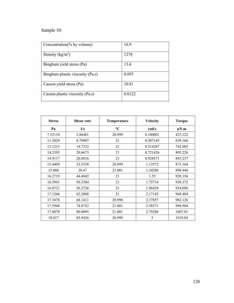
120
Sample 10:
Concentration(% by volume) 16.9
Density (kg/m3) 1278
Bingham yield stress (Pa) 13.6
Bingham plastic viscosity (Pa.s) 0.055
Casson yield stress (Pa) 10.81
Casson plastic viscosity (Pa.s) 0.0122
Stress Shear rate Temperature Velocity Torque
Pa 1/s °C rad/s µN.m
7.52134 2.86481 20.999 0.100001 425.322
11.3029 8.79907 21 0.307145 639.166
13.1215 14.7332 21 0.514287 742.005
14.2395 20.6673 21 0.721426 805.226
14.9117 26.6016 21 0.928571 843.237
15.4409 32.5358 20.999 1.13572 873.164
15.888 38.47 21.001 1.34286 898.446
16.2719 44.4042 21 1.55 920.156
16.5941 50.3384 21 1.75714 938.372
16.8721 56.2726 21 1.96429 954.096
17.1266 62.2068 21 2.17143 968.484
17.3678 68.1411 20.998 2.37857 982.126
17.5948 74.0752 21.001 2.58571 994.964
17.8078 80.0095 21.001 2.79286 1007.01
18.017 85.9436 20.999 3 1018.84

121
Sample 11:
Concentration(% by volume) 16.7
Density (kg/m3) 1275
Bingham yield stress (Pa) 14.1
Bingham plastic viscosity (Pa.s) 0.06
Casson yield stress (Pa) 11.2
Casson plastic viscosity (Pa.s) 0.013
Stress Shear rate Temperature Velocity Torque
Pa 1/s °C rad/s µN.m
7.730 2.865 20.089 0.100 437.135
11.599 8.799 20.099 0.307 655.889
13.407 14.733 20.101 0.514 758.132
14.656 20.667 20.099 0.721 828.787
15.595 26.602 20.100 0.929 881.853
16.178 32.536 20.099 1.136 914.845
16.651 38.470 20.100 1.343 941.617
17.048 44.404 20.100 1.550 964.059
17.388 50.338 20.100 1.757 983.290
17.692 56.273 20.100 1.964 1000.450
17.971 62.207 20.099 2.171 1016.230
18.229 68.141 20.099 2.379 1030.850
18.474 74.075 20.103 2.586 1044.670
18.708 80.010 20.099 2.793 1057.900
18.930 85.944 20.100 3.000 1070.490
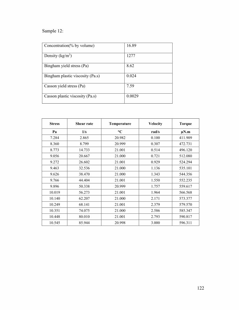
122
Sample 12:
Concentration(% by volume) 16.89
Density (kg/m3) 1277
Bingham yield stress (Pa) 8.62
Bingham plastic viscosity (Pa.s) 0.024
Casson yield stress (Pa) 7.59
Casson plastic viscosity (Pa.s) 0.0029
Stress Shear rate Temperature Velocity Torque
Pa 1/s °C rad/s µN.m
7.284 2.865 20.982 0.100 411.909
8.360 8.799 20.999 0.307 472.731
8.773 14.733 21.001 0.514 496.120
9.056 20.667 21.000 0.721 512.080
9.272 26.602 21.001 0.929 524.294
9.463 32.536 21.000 1.136 535.101
9.626 38.470 21.000 1.343 544.356
9.766 44.404 21.001 1.550 552.235
9.896 50.338 20.999 1.757 559.617
10.019 56.273 21.001 1.964 566.568
10.140 62.207 21.000 2.171 573.377
10.249 68.141 21.001 2.379 579.570
10.351 74.075 21.000 2.586 585.347
10.448 80.010 21.001 2.793 590.817
10.545 85.944 20.998 3.000 596.311
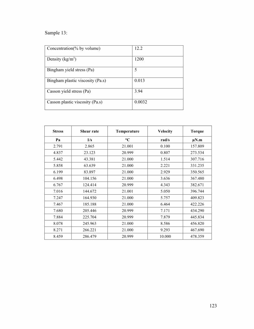
123
Sample 13:
Concentration(% by volume) 12.2
Density (kg/m3) 1200
Bingham yield stress (Pa) 5
Bingham plastic viscosity (Pa.s) 0.013
Casson yield stress (Pa) 3.94
Casson plastic viscosity (Pa.s) 0.0032
Stress Shear rate Temperature Velocity Torque
Pa 1/s °C rad/s µN.m
2.791 2.865 21.001 0.100 157.809
4.837 23.123 20.999 0.807 273.534
5.442 43.381 21.000 1.514 307.716
5.858 63.639 21.000 2.221 331.235
6.199 83.897 21.000 2.929 350.565
6.498 104.156 21.000 3.636 367.480
6.767 124.414 20.999 4.343 382.671
7.016 144.672 21.001 5.050 396.744
7.247 164.930 21.000 5.757 409.823
7.467 185.188 21.000 6.464 422.226
7.680 205.446 20.999 7.171 434.290
7.884 225.704 20.999 7.879 445.834
8.078 245.963 21.000 8.586 456.820
8.271 266.221 21.000 9.293 467.690
8.459 286.479 20.999 10.000 478.359

124
Sample 14:
Concentration(% by volume) 14.7
Density (kg/m3) 1241
Bingham yield stress (Pa) 7.84
Bingham plastic viscosity (Pa.s) 0.026
Casson yield stress (Pa) 6.244
Casson plastic viscosity (Pa.s) 0.0054
Stress Shear rate Temperature Velocity Torque
Pa 1/s °C rad/s µN.m
4.128 2.865 21.200 0.100 233.433
5.585 6.753 21.200 0.236 315.805
6.375 10.641 21.201 0.371 360.497
6.929 14.529 21.199 0.507 391.828
7.327 18.417 21.200 0.643 414.325
7.662 22.304 21.201 0.779 433.263
8.019 26.192 21.198 0.914 453.482
8.299 30.080 21.200 1.050 469.297
8.474 33.968 21.200 1.186 479.220
8.623 37.856 21.201 1.321 487.596
8.762 41.744 21.200 1.457 495.488
8.889 45.632 21.200 1.593 502.655
9.009 49.520 21.199 1.729 509.440
9.122 53.408 21.200 1.864 515.814
9.230 57.296 21.199 2.000 521.957

125
Sample 15:
Concentration(% by volume) 15.4
Density (kg/m3) 1252
Bingham yield stress (Pa) 8.9
Bingham plastic viscosity (Pa.s) 0.024
Casson yield stress (Pa) 7.47
Casson plastic viscosity (Pa.s) 0.004
Stress Shear rate Temperature Velocity Torque
Pa 1/s °C rad/s µN.m
3.303 2.865 22.500 0.100 186.804
6.150 6.753 22.500 0.236 347.747
7.058 10.641 22.498 0.371 399.116
7.724 14.529 22.501 0.507 436.781
8.256 18.417 22.501 0.643 466.856
8.626 22.304 22.500 0.779 487.766
8.949 26.192 22.501 0.914 506.067
9.326 30.080 22.499 1.050 527.385
9.583 33.968 22.499 1.186 541.931
9.737 37.856 22.500 1.321 550.616
9.862 41.744 22.498 1.457 557.689
9.978 45.632 22.500 1.593 564.223
10.082 49.520 22.501 1.729 570.100
10.183 53.408 22.499 1.864 575.806
10.278 57.296 22.499 2.000 581.193
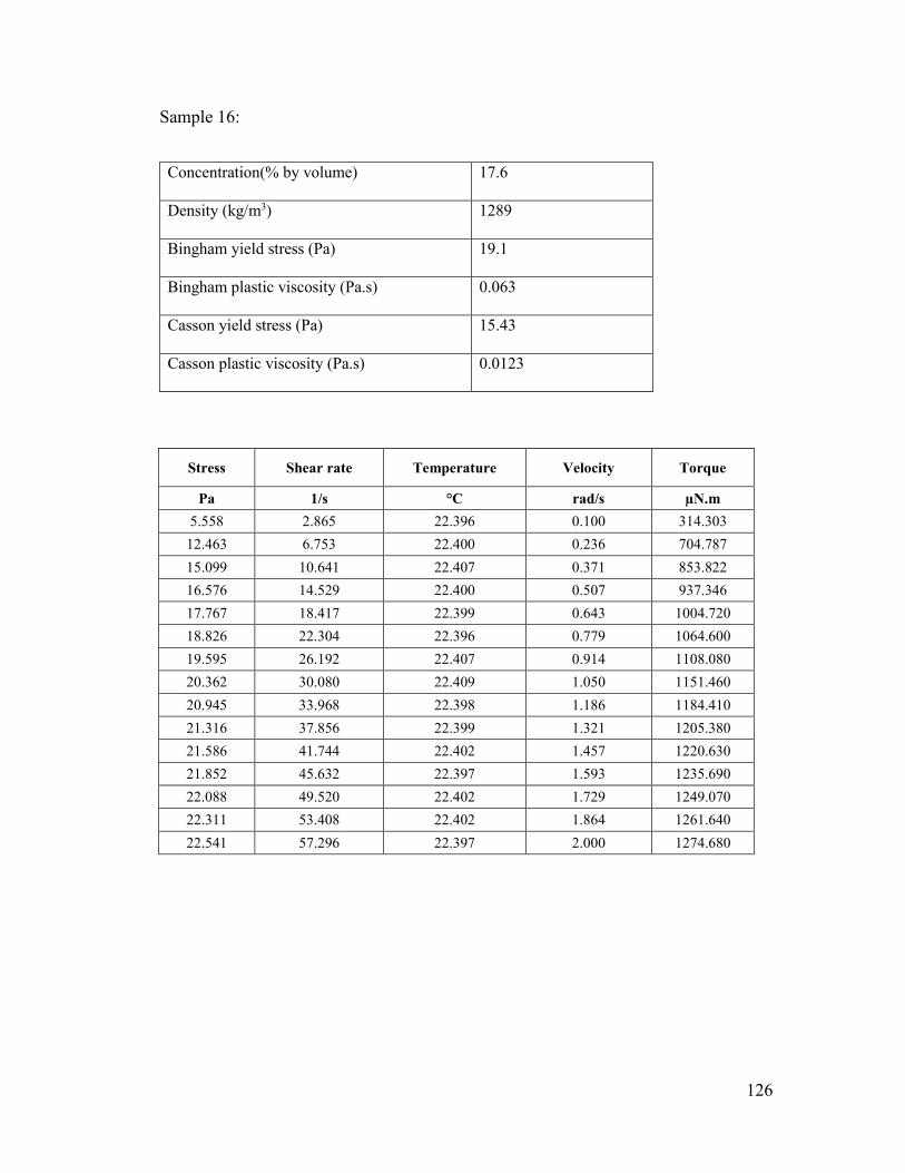
126
Sample 16:
Concentration(% by volume) 17.6
Density (kg/m3) 1289
Bingham yield stress (Pa) 19.1
Bingham plastic viscosity (Pa.s) 0.063
Casson yield stress (Pa) 15.43
Casson plastic viscosity (Pa.s) 0.0123
Stress Shear rate Temperature Velocity Torque
Pa 1/s °C rad/s µN.m
5.558 2.865 22.396 0.100 314.303
12.463 6.753 22.400 0.236 704.787
15.099 10.641 22.407 0.371 853.822
16.576 14.529 22.400 0.507 937.346
17.767 18.417 22.399 0.643 1004.720
18.826 22.304 22.396 0.779 1064.600
19.595 26.192 22.407 0.914 1108.080
20.362 30.080 22.409 1.050 1151.460
20.945 33.968 22.398 1.186 1184.410
21.316 37.856 22.399 1.321 1205.380
21.586 41.744 22.402 1.457 1220.630
21.852 45.632 22.397 1.593 1235.690
22.088 49.520 22.402 1.729 1249.070
22.311 53.408 22.402 1.864 1261.640
22.541 57.296 22.397 2.000 1274.680

127
Sample 17:
Concentration(% by volume) 20.1
Density (kg/m3) 1331
Bingham yield stress (Pa) 27.3
Bingham plastic viscosity (Pa.s) 0.145
Casson yield stress (Pa) 19.7
Casson plastic viscosity (Pa.s) 0.04
Stress Shear rate Temperature Velocity Torque
Pa 1/s °C rad/s µN.m
6.994 2.865 23.302 0.100 395.507
17.432 6.753 23.299 0.236 985.735
21.051 10.641 23.301 0.371 1190.380
23.983 14.529 23.299 0.507 1356.190
25.988 18.417 23.301 0.643 1469.560
27.615 22.304 23.299 0.779 1561.610
29.091 26.192 23.300 0.914 1645.050
30.372 30.080 23.301 1.050 1717.480
31.425 33.968 23.301 1.186 1777.040
32.472 37.856 23.299 1.321 1836.220
33.509 41.744 23.301 1.457 1894.870
34.304 45.632 23.300 1.593 1939.850
34.923 49.520 23.299 1.729 1974.830
35.473 53.408 23.302 1.864 2005.940
35.953 57.296 23.299 2.000 2033.070

128
Sample 18:
Concentration(% by volume) 19.4
Density (kg/m3) 1318
Bingham yield stress (Pa) 19
Bingham plastic viscosity (Pa.s) 0.083
Casson yield stress (Pa) 16.17
Casson plastic viscosity (Pa.s) 0.011
Stress Shear rate Temperature Velocity Torque
Pa 1/s °C rad/s µN.m
9.963 2.865 23.600 0.100 563.419
14.054 6.753 23.600 0.236 794.760
16.639 10.641 23.600 0.371 940.889
18.371 14.529 23.600 0.507 1038.850
19.338 18.417 23.599 0.643 1093.560
20.322 22.304 23.601 0.779 1149.180
21.065 26.192 23.599 0.914 1191.200
21.506 30.080 23.601 1.050 1216.150
21.874 33.968 23.601 1.186 1236.970
22.222 37.856 23.600 1.321 1256.600
22.543 41.744 23.599 1.457 1274.760
22.846 45.632 23.600 1.593 1291.930
23.142 49.520 23.600 1.729 1308.630
23.424 53.408 23.599 1.864 1324.570
23.699 57.296 23.600 2.000 1340.140

129
Sample 19:
Concentration(% by volume) 21.73
Density (kg/m3) 1357
Bingham yield stress (Pa) 30
Bingham plastic viscosity (Pa.s) 0.98
Casson yield stress (Pa) 25.65
Casson plastic viscosity (Pa.s) 0.15
Stress Shear rate Temperature Velocity Torque
Pa 1/s °C rad/s µN.m
14.144 0.358 24.201 0.100 799.824
21.357 0.844 24.199 0.236 1207.680
25.595 1.330 24.201 0.371 1447.380
27.892 1.816 24.201 0.507 1577.270
29.995 2.302 24.205 0.643 1696.180
31.231 2.788 24.198 0.779 1766.090
32.298 3.274 24.197 0.914 1826.390
33.484 3.760 24.203 1.050 1893.490
34.153 4.246 24.200 1.186 1931.300
34.714 4.732 24.200 1.321 1963.000
35.239 5.218 24.202 1.457 1992.720
35.719 5.704 24.198 1.593 2019.880
36.183 6.190 24.200 1.729 2046.070
36.619 6.676 24.202 1.864 2070.780
37.041 7.162 24.198 2.000 2094.620

130
Sample 20:
Concentration(% by volume) 21.73
Density (kg/m3) 1357
Bingham yield stress (Pa) 19.5
Bingham plastic viscosity (Pa.s) 0.45
Casson yield stress (Pa) 12.8
Casson plastic viscosity (Pa.s) 0.157
Stress Shear rate Temperature Velocity Torque
Pa 1/s °C rad/s µN.m
13.8182 2.86483 23.2 0.100001 781.401
15.9538 4.70649 23.201 0.164288 902.169
19.0855 6.5481 23.2 0.228572 1079.26
21.5917 8.38974 23.199 0.292857 1220.98
23.2561 10.2314 23.201 0.357144 1315.1
24.6405 12.073 23.201 0.421429 1393.39
25.9118 13.9147 23.199 0.485714 1465.28
27.1444 15.7563 23.2 0.55 1534.98
27.9679 17.598 23.202 0.614286 1581.55
28.6332 19.4396 23.2 0.678571 1619.17
29.3195 21.2813 23.2 0.742857 1657.98
30.2032 23.1229 23.2 0.807143 1707.95
30.9063 24.9646 23.2 0.871429 1747.71
31.3532 26.8062 23.198 0.935715 1772.98
31.7095 28.6479 23.201 1 1793.13

131
Sample 21:
Concentration(% by volume) 19.5
Density (kg/m3) 1320
Bingham yield stress (Pa) 12.2
Bingham plastic viscosity (Pa.s) 0.45
Casson yield stress (Pa) 8.49
Casson plastic viscosity (Pa.s) 0.131
Stress Shear rate Temperature Velocity Torque
Pa 1/s °C rad/s µN.m
12.677 4.000 23.600 0.140 716.843
13.233 4.786 23.600 0.167 748.328
13.900 5.571 23.600 0.194 786.013
14.542 6.357 23.600 0.222 822.356
15.146 7.143 23.599 0.249 856.505
15.603 7.929 23.600 0.277 882.306
15.935 8.714 23.600 0.304 901.093
16.237 9.500 23.600 0.332 918.206
16.508 10.286 23.600 0.359 933.497
16.784 11.071 23.600 0.386 949.114
17.093 11.857 23.600 0.414 966.577
17.490 12.643 23.600 0.441 989.011
17.804 13.429 23.600 0.469 1006.810
18.011 14.214 23.600 0.496 1018.490
18.175 15.000 23.600 0.524 1027.750
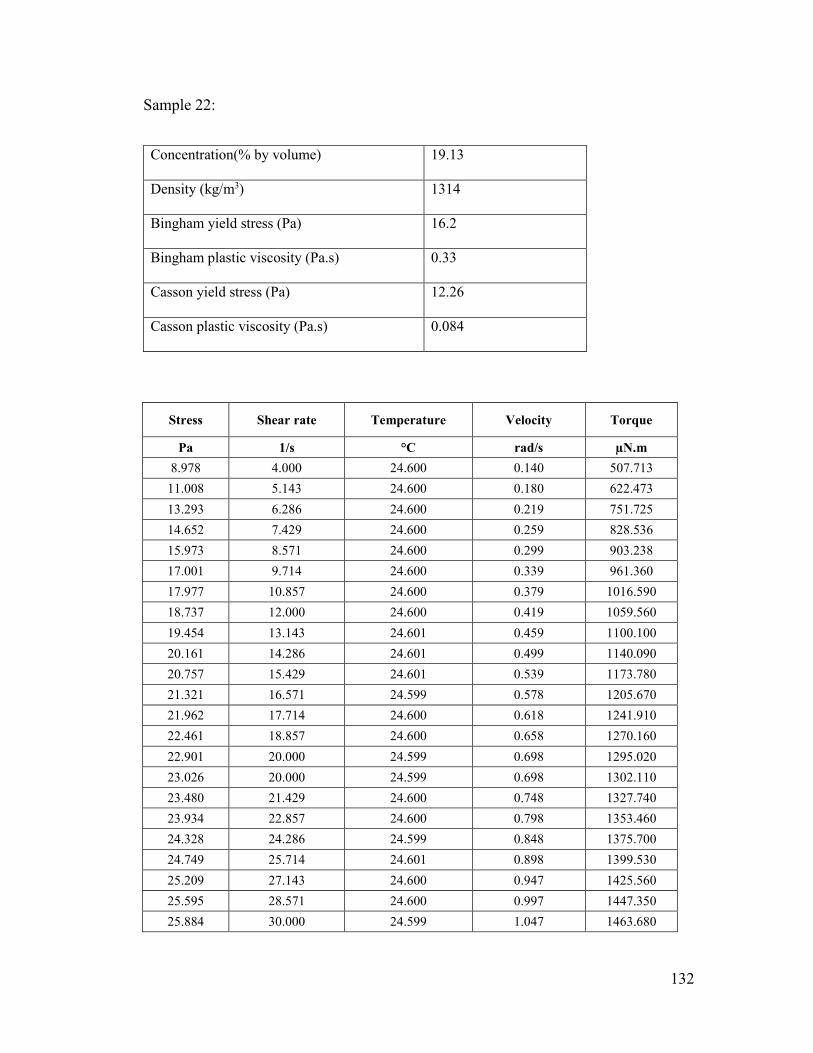
132
Sample 22:
Concentration(% by volume) 19.13
Density (kg/m3) 1314
Bingham yield stress (Pa) 16.2
Bingham plastic viscosity (Pa.s) 0.33
Casson yield stress (Pa) 12.26
Casson plastic viscosity (Pa.s) 0.084
Stress Shear rate Temperature Velocity Torque
Pa 1/s °C rad/s µN.m
8.978 4.000 24.600 0.140 507.713
11.008 5.143 24.600 0.180 622.473
13.293 6.286 24.600 0.219 751.725
14.652 7.429 24.600 0.259 828.536
15.973 8.571 24.600 0.299 903.238
17.001 9.714 24.600 0.339 961.360
17.977 10.857 24.600 0.379 1016.590
18.737 12.000 24.600 0.419 1059.560
19.454 13.143 24.601 0.459 1100.100
20.161 14.286 24.601 0.499 1140.090
20.757 15.429 24.601 0.539 1173.780
21.321 16.571 24.599 0.578 1205.670
21.962 17.714 24.600 0.618 1241.910
22.461 18.857 24.600 0.658 1270.160
22.901 20.000 24.599 0.698 1295.020
23.026 20.000 24.599 0.698 1302.110
23.480 21.429 24.600 0.748 1327.740
23.934 22.857 24.600 0.798 1353.460
24.328 24.286 24.599 0.848 1375.700
24.749 25.714 24.601 0.898 1399.530
25.209 27.143 24.600 0.947 1425.560
25.595 28.571 24.600 0.997 1447.350
25.884 30.000 24.599 1.047 1463.680

133
Sample 23:
Concentration(% by volume) 19.13
Density (kg/m3) 1314
Bingham yield stress (Pa) 13.5
Bingham plastic viscosity (Pa.s) 0.46
Casson yield stress (Pa) 8.74
Casson plastic viscosity (Pa.s) 0.165
Stress Shear rate Temperature Velocity Torque
Pa 1/s °C rad/s µN.m
8.978 4.000 24.600 0.140 507.713
11.008 5.143 24.600 0.180 622.473
13.293 6.286 24.600 0.219 751.725
14.652 7.429 24.600 0.259 828.536
15.973 8.571 24.600 0.299 903.238
17.001 9.714 24.600 0.339 961.360
17.977 10.857 24.600 0.379 1016.590
18.737 12.000 24.600 0.419 1059.560
19.454 13.143 24.601 0.459 1100.100
20.161 14.286 24.601 0.499 1140.090
20.757 15.429 24.601 0.539 1173.780
21.321 16.571 24.599 0.578 1205.670
21.962 17.714 24.600 0.618 1241.910
22.461 18.857 24.600 0.658 1270.160
22.901 20.000 24.599 0.698 1295.020
23.026 20.000 24.599 0.698 1302.110
23.480 21.429 24.600 0.748 1327.740
23.934 22.857 24.600 0.798 1353.460
24.328 24.286 24.599 0.848 1375.700
24.749 25.714 24.601 0.898 1399.530
25.209 27.143 24.600 0.947 1425.560
25.595 28.571 24.600 0.997 1447.350
25.884 30.000 24.599 1.047 1463.680

134
Sample 24:
Concentration(% by volume) 21.1
Density (kg/m3) 1347
Bingham yield stress (Pa) 20.6
Bingham plastic viscosity (Pa.s) 0.42
Casson yield stress (Pa) 16.37
Casson plastic viscosity (Pa.s) 0.097
Stress Shear rate Temperature Velocity Torque
Pa 1/s °C rad/s µN.m
24.288 10.000 24.002 0.349 1373.450
24.852 11.429 24.000 0.399 1405.320
25.759 12.857 24.001 0.449 1456.660
26.650 14.286 24.000 0.499 1507.000
27.731 15.714 24.001 0.549 1568.130
28.541 17.143 24.000 0.598 1613.980
28.998 18.571 24.000 0.648 1639.770
29.435 20.000 24.001 0.698 1664.530
29.812 21.429 23.998 0.748 1685.800
30.264 22.857 24.001 0.798 1711.400
30.759 24.286 24.000 0.848 1739.350
31.479 25.714 24.000 0.898 1780.090
32.038 27.143 23.999 0.947 1811.730
32.380 28.571 23.999 0.997 1831.060
32.683 30.000 24.001 1.047 1848.170

135
Sample 25:
Concentration(% by volume) 19.6
Density (kg/m3) 1322
Bingham yield stress (Pa) 17.6
Bingham plastic viscosity (Pa.s) 0.12
Casson yield stress (Pa) 14.1
Casson plastic viscosity (Pa.s) 0.024
Stress Shear rate Temperature Velocity Torque
Pa 1/s °C rad/s µN.m
16.297 10.000 24.301 0.349 921.551
16.717 11.429 24.300 0.399 945.333
17.372 12.857 24.298 0.449 982.364
17.939 14.286 24.301 0.499 1014.450
18.359 15.714 24.299 0.549 1038.200
18.716 17.143 24.299 0.598 1058.370
19.062 18.571 24.301 0.648 1077.930
19.426 20.000 24.298 0.698 1098.490
19.857 21.429 24.300 0.748 1122.900
20.345 22.857 24.299 0.798 1150.500
20.639 24.286 24.299 0.848 1167.110
20.863 25.714 24.302 0.898 1179.750
21.062 27.143 24.299 0.947 1191.000
21.247 28.571 24.300 0.997 1201.470
21.414 30.000 24.300 1.047 1210.910
21.440 30.000 24.300 1.047 1212.420
21.623 31.429 24.300 1.097 1222.730
21.795 32.857 24.298 1.147 1232.490
21.947 34.286 24.300 1.197 1241.080
22.093 35.714 24.300 1.247 1249.300
22.256 37.143 24.299 1.297 1258.530
22.416 38.571 24.301 1.346 1267.570
22.569 40.000 24.300 1.396 1276.270

136
Sample 26:
Concentration(% by volume) 17.1
Density (kg/m3) 1280
Bingham yield stress (Pa) 15.1
Bingham plastic viscosity (Pa.s) 0.11
Casson yield stress (Pa) 11.8
Casson plastic viscosity (Pa.s) 0.026
Stress Shear rate Temperature Velocity Torque
Pa 1/s °C rad/s µN.m
12.096 10.000 23.000 0.349 683.994
12.234 11.579 23.000 0.404 691.791
12.644 13.158 22.999 0.459 714.991
13.114 14.737 23.001 0.514 741.553
13.542 16.316 22.999 0.570 765.754
13.920 17.895 23.001 0.625 787.141
14.316 19.474 23.001 0.680 809.563
14.708 21.053 22.999 0.735 831.701
15.105 22.632 23.001 0.790 854.167
15.431 24.211 23.000 0.845 872.618
15.696 25.790 23.000 0.900 887.584
15.936 27.368 22.999 0.955 901.165
16.168 28.947 23.000 1.010 914.251
16.370 30.526 22.999 1.066 925.725
16.563 32.105 23.000 1.121 936.590
16.754 33.684 23.000 1.176 947.431
16.933 35.263 23.001 1.231 957.509
17.106 36.842 23.001 1.286 967.339
17.269 38.421 23.000 1.341 976.538
17.415 40.000 23.000 1.396 984.776
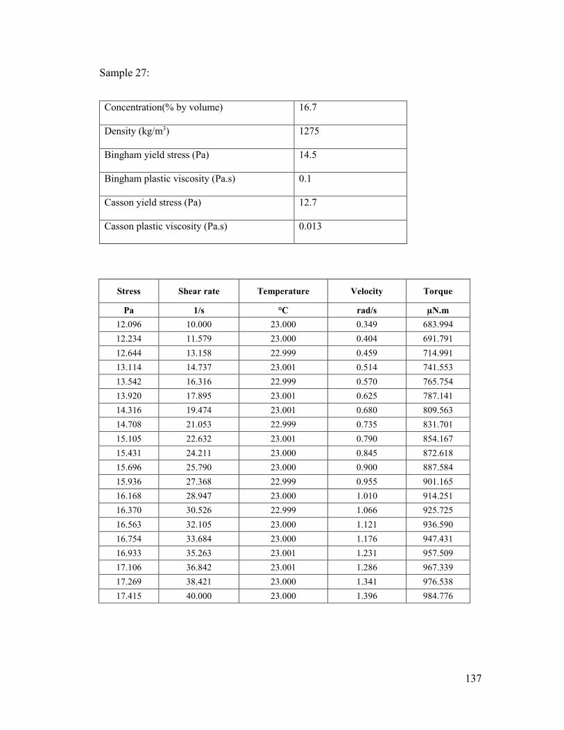
137
Sample 27:
Concentration(% by volume) 16.7
Density (kg/m3) 1275
Bingham yield stress (Pa) 14.5
Bingham plastic viscosity (Pa.s) 0.1
Casson yield stress (Pa) 12.7
Casson plastic viscosity (Pa.s) 0.013
Stress Shear rate Temperature Velocity Torque
Pa 1/s °C rad/s µN.m
12.096 10.000 23.000 0.349 683.994
12.234 11.579 23.000 0.404 691.791
12.644 13.158 22.999 0.459 714.991
13.114 14.737 23.001 0.514 741.553
13.542 16.316 22.999 0.570 765.754
13.920 17.895 23.001 0.625 787.141
14.316 19.474 23.001 0.680 809.563
14.708 21.053 22.999 0.735 831.701
15.105 22.632 23.001 0.790 854.167
15.431 24.211 23.000 0.845 872.618
15.696 25.790 23.000 0.900 887.584
15.936 27.368 22.999 0.955 901.165
16.168 28.947 23.000 1.010 914.251
16.370 30.526 22.999 1.066 925.725
16.563 32.105 23.000 1.121 936.590
16.754 33.684 23.000 1.176 947.431
16.933 35.263 23.001 1.231 957.509
17.106 36.842 23.001 1.286 967.339
17.269 38.421 23.000 1.341 976.538
17.415 40.000 23.000 1.396 984.776
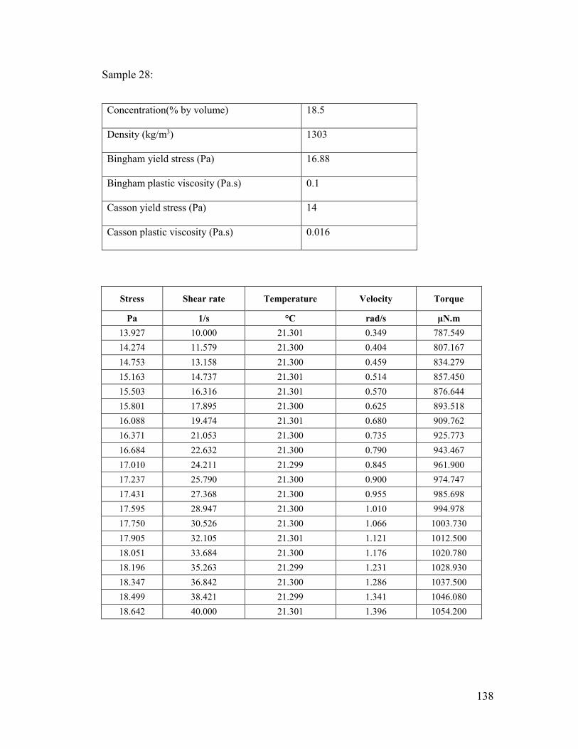
138
Sample 28:
Concentration(% by volume) 18.5
Density (kg/m3) 1303
Bingham yield stress (Pa) 16.88
Bingham plastic viscosity (Pa.s) 0.1
Casson yield stress (Pa) 14
Casson plastic viscosity (Pa.s) 0.016
Stress Shear rate Temperature Velocity Torque
Pa 1/s °C rad/s µN.m
13.927 10.000 21.301 0.349 787.549
14.274 11.579 21.300 0.404 807.167
14.753 13.158 21.300 0.459 834.279
15.163 14.737 21.301 0.514 857.450
15.503 16.316 21.301 0.570 876.644
15.801 17.895 21.300 0.625 893.518
16.088 19.474 21.301 0.680 909.762
16.371 21.053 21.300 0.735 925.773
16.684 22.632 21.300 0.790 943.467
17.010 24.211 21.299 0.845 961.900
17.237 25.790 21.300 0.900 974.747
17.431 27.368 21.300 0.955 985.698
17.595 28.947 21.300 1.010 994.978
17.750 30.526 21.300 1.066 1003.730
17.905 32.105 21.301 1.121 1012.500
18.051 33.684 21.300 1.176 1020.780
18.196 35.263 21.299 1.231 1028.930
18.347 36.842 21.300 1.286 1037.500
18.499 38.421 21.299 1.341 1046.080
18.642 40.000 21.301 1.396 1054.200
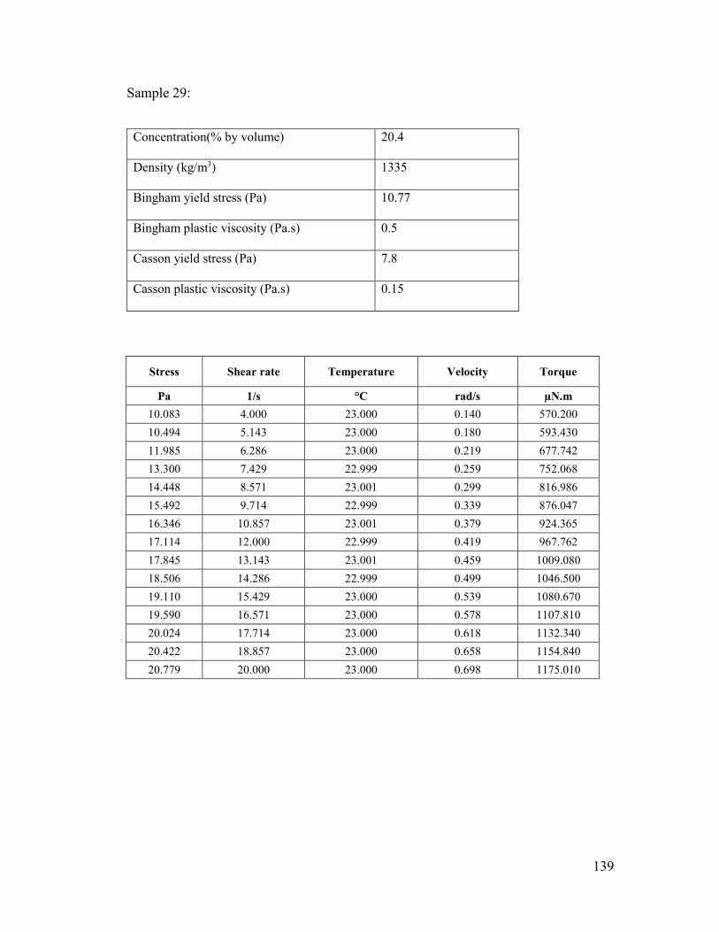
139
Sample 29:
Concentration(% by volume) 20.4
Density (kg/m3) 1335
Bingham yield stress (Pa) 10.77
Bingham plastic viscosity (Pa.s) 0.5
Casson yield stress (Pa) 7.8
Casson plastic viscosity (Pa.s) 0.15
Stress Shear rate Temperature Velocity Torque
Pa 1/s °C rad/s µN.m
10.083 4.000 23.000 0.140 570.200
10.494 5.143 23.000 0.180 593.430
11.985 6.286 23.000 0.219 677.742
13.300 7.429 22.999 0.259 752.068
14.448 8.571 23.001 0.299 816.986
15.492 9.714 22.999 0.339 876.047
16.346 10.857 23.001 0.379 924.365
17.114 12.000 22.999 0.419 967.762
17.845 13.143 23.001 0.459 1009.080
18.506 14.286 22.999 0.499 1046.500
19.110 15.429 23.000 0.539 1080.670
19.590 16.571 23.000 0.578 1107.810
20.024 17.714 23.000 0.618 1132.340
20.422 18.857 23.000 0.658 1154.840
20.779 20.000 23.000 0.698 1175.010
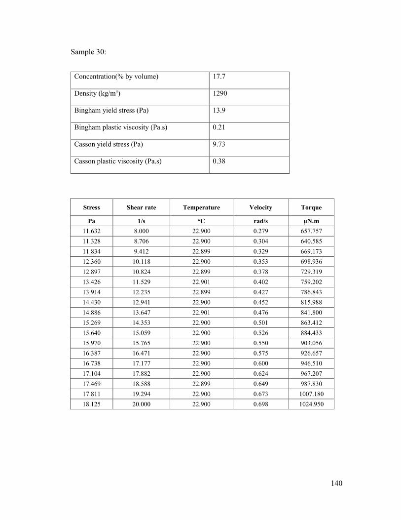
140
Sample 30:
Concentration(% by volume) 17.7
Density (kg/m3) 1290
Bingham yield stress (Pa) 13.9
Bingham plastic viscosity (Pa.s) 0.21
Casson yield stress (Pa) 9.73
Casson plastic viscosity (Pa.s) 0.38
Stress Shear rate Temperature Velocity Torque
Pa 1/s °C rad/s µN.m
11.632 8.000 22.900 0.279 657.757
11.328 8.706 22.900 0.304 640.585
11.834 9.412 22.899 0.329 669.173
12.360 10.118 22.900 0.353 698.936
12.897 10.824 22.899 0.378 729.319
13.426 11.529 22.901 0.402 759.202
13.914 12.235 22.899 0.427 786.843
14.430 12.941 22.900 0.452 815.988
14.886 13.647 22.901 0.476 841.800
15.269 14.353 22.900 0.501 863.412
15.640 15.059 22.900 0.526 884.433
15.970 15.765 22.900 0.550 903.056
16.387 16.471 22.900 0.575 926.657
16.738 17.177 22.900 0.600 946.510
17.104 17.882 22.900 0.624 967.207
17.469 18.588 22.899 0.649 987.830
17.811 19.294 22.900 0.673 1007.180
18.125 20.000 22.900 0.698 1024.950
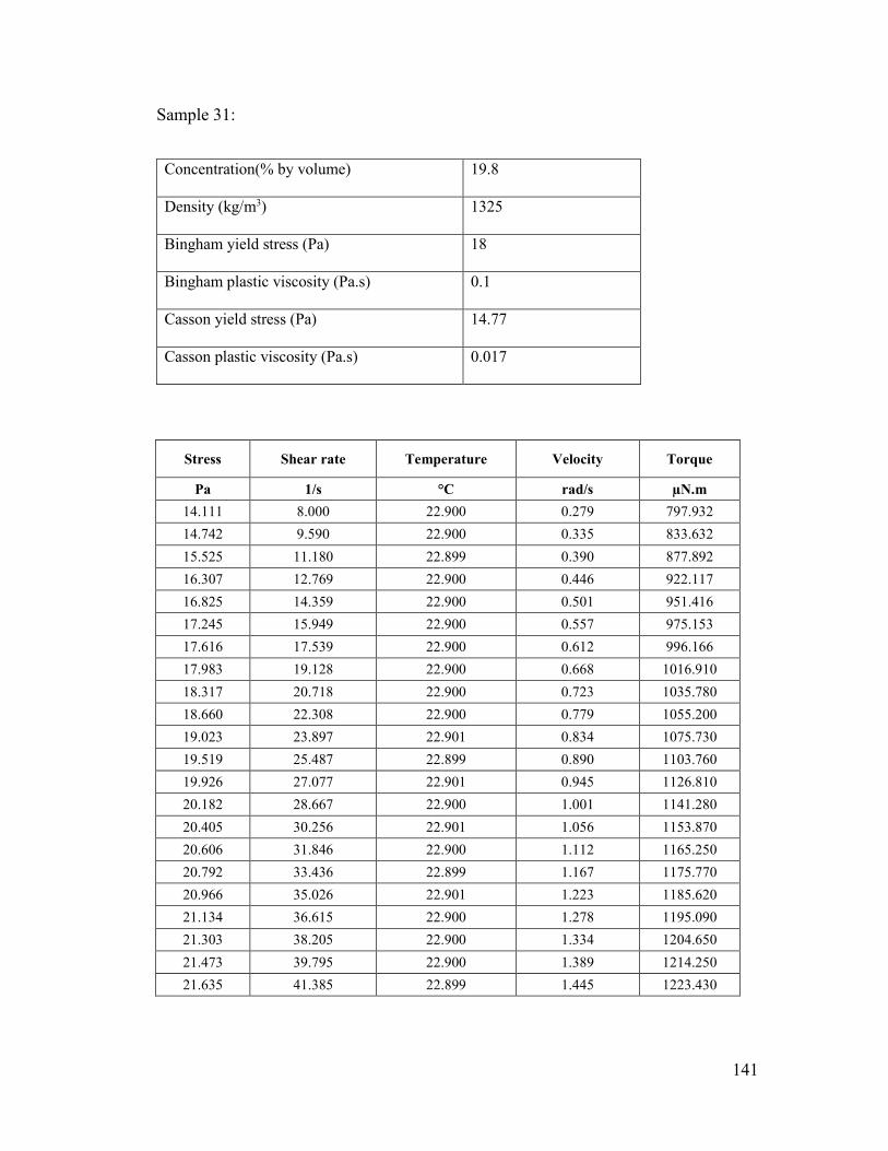
141
Sample 31:
Concentration(% by volume) 19.8
Density (kg/m3) 1325
Bingham yield stress (Pa) 18
Bingham plastic viscosity (Pa.s) 0.1
Casson yield stress (Pa) 14.77
Casson plastic viscosity (Pa.s) 0.017
Stress Shear rate Temperature Velocity Torque
Pa 1/s °C rad/s µN.m
14.111 8.000 22.900 0.279 797.932
14.742 9.590 22.900 0.335 833.632
15.525 11.180 22.899 0.390 877.892
16.307 12.769 22.900 0.446 922.117
16.825 14.359 22.900 0.501 951.416
17.245 15.949 22.900 0.557 975.153
17.616 17.539 22.900 0.612 996.166
17.983 19.128 22.900 0.668 1016.910
18.317 20.718 22.900 0.723 1035.780
18.660 22.308 22.900 0.779 1055.200
19.023 23.897 22.901 0.834 1075.730
19.519 25.487 22.899 0.890 1103.760
19.926 27.077 22.901 0.945 1126.810
20.182 28.667 22.900 1.001 1141.280
20.405 30.256 22.901 1.056 1153.870
20.606 31.846 22.900 1.112 1165.250
20.792 33.436 22.899 1.167 1175.770
20.966 35.026 22.901 1.223 1185.620
21.134 36.615 22.900 1.278 1195.090
21.303 38.205 22.900 1.334 1204.650
21.473 39.795 22.900 1.389 1214.250
21.635 41.385 22.899 1.445 1223.430

142
Sample 32:
Concentration(% by volume) 20.1
Density (kg/m3) 1331
Bingham yield stress (Pa) 22.4
Bingham plastic viscosity (Pa.s) 0.124
Casson yield stress (Pa) 18.4
Casson plastic viscosity (Pa.s) 0.024
Stress Shear rate Temperature Velocity Torque
Pa 1/s °C rad/s µN.m
17.111 8.000 24.000 0.279 967.588
17.130 8.857 24.000 0.309 968.671
17.757 9.714 23.999 0.339 1004.160
18.373 10.572 24.001 0.369 1038.950
19.008 11.429 23.999 0.399 1074.870
19.568 12.286 24.000 0.429 1106.560
20.113 13.143 24.001 0.459 1137.340
20.636 14.000 23.999 0.489 1166.920
21.154 14.857 24.000 0.519 1196.240
21.559 15.714 24.000 0.549 1219.150
21.980 16.571 24.000 0.578 1242.920
22.343 17.429 24.000 0.608 1263.480
22.717 18.286 24.001 0.638 1284.630
23.094 19.143 23.999 0.668 1305.920
23.417 20.000 24.001 0.698 1324.220
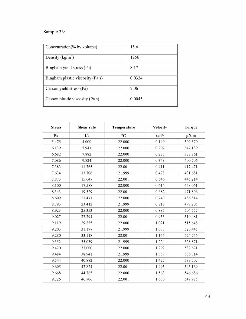
143
Sample 33:
Concentration(% by volume) 15.6
Density (kg/m3) 1256
Bingham yield stress (Pa) 8.17
Bingham plastic viscosity (Pa.s) 0.0324
Casson yield stress (Pa) 7.06
Casson plastic viscosity (Pa.s) 0.0045
Stress Shear rate Temperature Velocity Torque
Pa 1/s °C rad/s µN.m
5.475 4.000 22.000 0.140 309.579
6.139 5.941 22.000 0.207 347.139
6.682 7.882 22.000 0.275 377.861
7.086 9.824 22.000 0.343 400.706
7.383 11.765 22.001 0.411 417.471
7.634 13.706 21.999 0.478 431.681
7.873 15.647 22.001 0.546 445.214
8.100 17.588 22.000 0.614 458.061
8.343 19.529 22.001 0.682 471.806
8.609 21.471 22.000 0.749 486.814
8.793 23.412 21.999 0.817 497.205
8.923 25.353 22.000 0.885 504.557
9.027 27.294 22.001 0.953 510.481
9.119 29.235 22.000 1.021 515.648
9.203 31.177 21.999 1.088 520.445
9.280 33.118 22.001 1.156 524.756
9.352 35.059 21.999 1.224 528.871
9.420 37.000 22.000 1.292 532.671
9.484 38.941 21.999 1.359 536.314
9.544 40.882 22.000 1.427 539.707
9.605 42.824 22.001 1.495 543.169
9.668 44.765 22.000 1.563 546.686
9.726 46.706 22.001 1.630 549.975
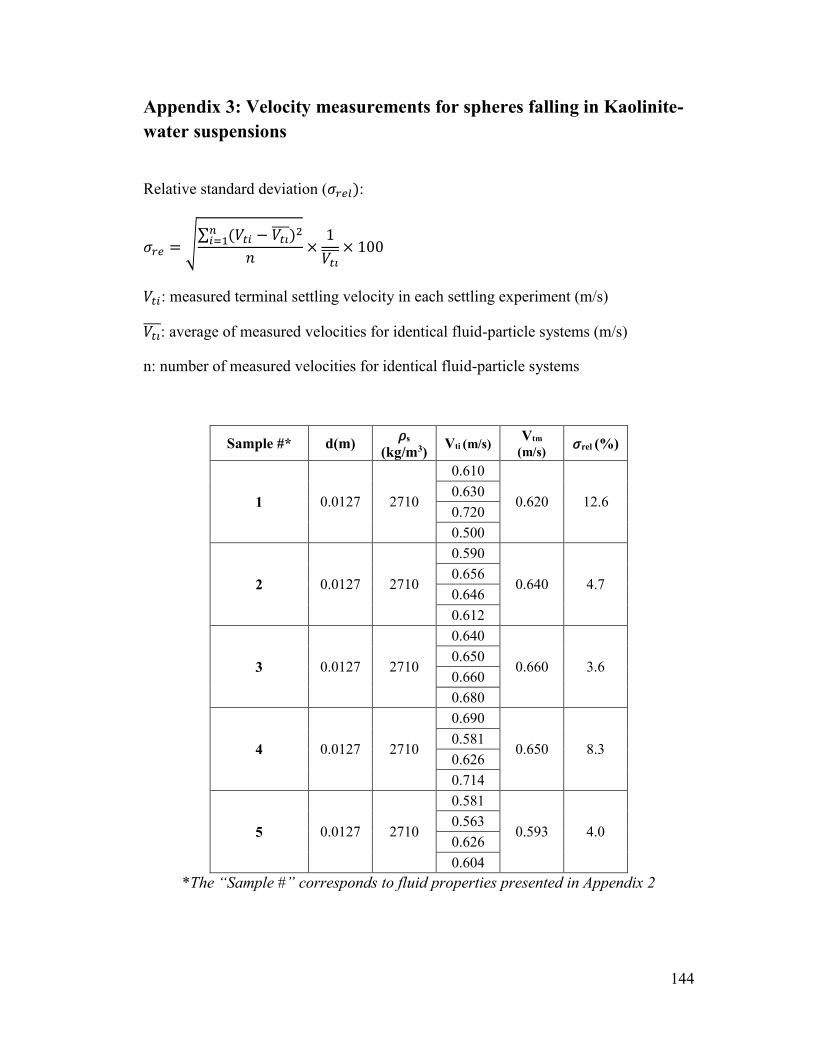
144
Appendix 3: Velocity measurements for spheres falling in Kaolinite-
water suspensions
Relative standard deviation (𝜎𝑟𝑒𝑙):
𝜎𝑟𝑒 = √∑ (𝑉𝑡𝑖 − 𝑉𝑡𝑖
)2𝑛𝑖=1
𝑛×
1
𝑉𝑡𝑖
× 100
𝑉𝑡𝑖: measured terminal settling velocity in each settling experiment (m/s)
𝑉𝑡𝑖 : average of measured velocities for identical fluid-particle systems (m/s)
n: number of measured velocities for identical fluid-particle systems
Sample #* d(m) 𝜌s
(kg/m3) Vti (m/s)
Vtm
(m/s) 𝜎rel (%)
1 0.0127 2710
0.610
0.620 12.6 0.630
0.720
0.500
2 0.0127 2710
0.590
0.640 4.7 0.656
0.646
0.612
3 0.0127 2710
0.640
0.660 3.6 0.650
0.660
0.680
4 0.0127 2710
0.690
0.650 8.3 0.581
0.626
0.714
5 0.0127 2710
0.581
0.593 4.0 0.563
0.626
0.604
*The “Sample #” corresponds to fluid properties presented in Appendix 2

145
Sample # d(m)
𝜌s
(kg/m3) Vti (m/s)
Vtm
(m/s) 𝜎rel (%)
6
0.0191 7697
1.549
1.472 3.5 1.418
1.433
1.489
0.0159 7722
1.374
1.293 4.2
1.333
1.340
1.327
1.140
1.241
0.0143 7684
1.270
1.270 2.8
1.314
1.213
1.301
1.252
0.0127 7841
1.150
1.181 2.2
1.136
1.170
1.218
1.196
1.191
1.186
1.213
1.170
0.0127 2710
0.022
0.028 13.7 0.030
0.032
0.027
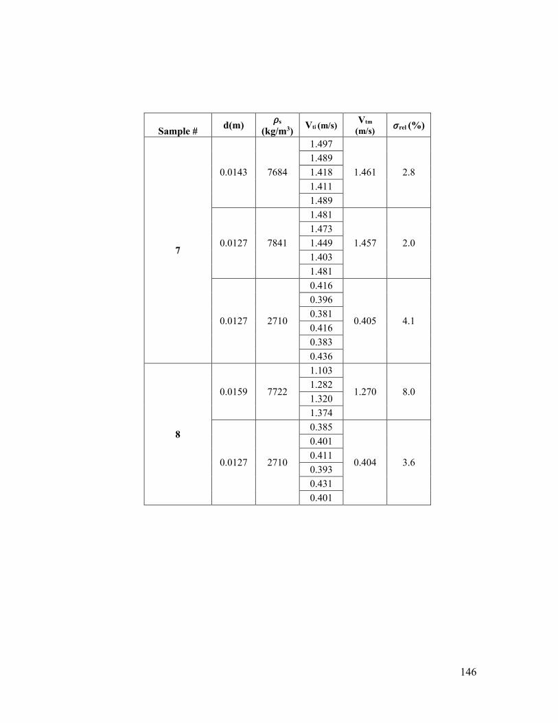
146
Sample # d(m)
𝜌s
(kg/m3) Vti (m/s)
Vtm
(m/s) 𝜎rel (%)
7
0.0143 7684
1.497
1.461 2.8
1.489
1.418
1.411
1.489
0.0127 7841
1.481
1.457 2.0
1.473
1.449
1.403
1.481
0.0127 2710
0.416
0.405 4.1
0.396
0.381
0.416
0.383
0.436
8
0.0159 7722
1.103
1.270 8.0 1.282
1.320
1.374
0.0127 2710
0.385
0.404 3.6
0.401
0.411
0.393
0.431
0.401
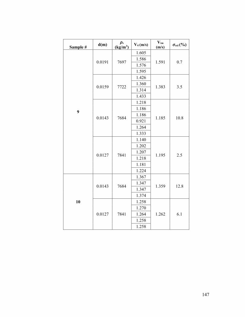
147
Sample # d(m)
𝜌s
(kg/m3) Vti (m/s)
Vtm
(m/s) 𝜎rel (%)
9
0.0191 7697
1.605
1.591 0.7 1.586
1.576
1.595
0.0159 7722
1.426
1.383 3.5 1.360
1.314
1.433
0.0143 7684
1.218
1.185 10.8
1.186
1.186
0.921
1.264
1.333
0.0127 7841
1.140
1.195 2.5
1.202
1.207
1.218
1.181
1.224
10
0.0143 7684
1.367
1.359 12.8 1.347
1.347
1.374
0.0127 7841
1.258
1.262 6.1
1.270
1.264
1.258
1.258
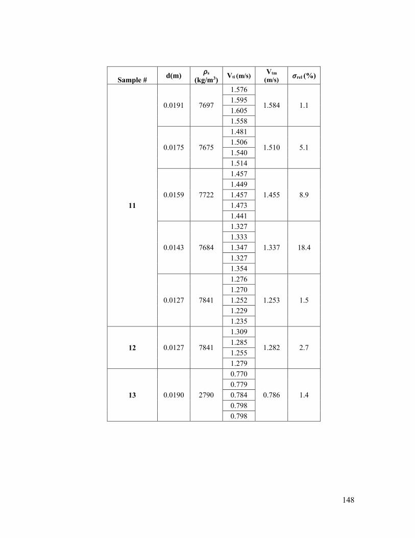
148
Sample # d(m)
𝜌s
(kg/m3) Vti (m/s)
Vtm
(m/s) 𝜎rel (%)
11
0.0191 7697
1.576
1.584 1.1 1.595
1.605
1.558
0.0175 7675
1.481
1.510 5.1 1.506
1.540
1.514
0.0159 7722
1.457
1.455 8.9
1.449
1.457
1.473
1.441
0.0143 7684
1.327
1.337 18.4
1.333
1.347
1.327
1.354
0.0127 7841
1.276
1.253 1.5
1.270
1.252
1.229
1.235
12 0.0127 7841
1.309
1.282 2.7 1.285
1.255
1.279
13 0.0190 2790
0.770
0.786 1.4
0.779
0.784
0.798
0.798
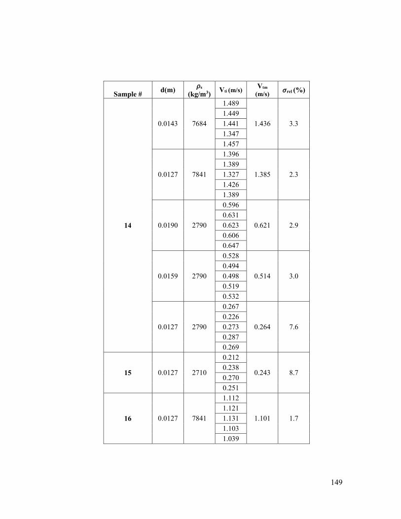
149
Sample # d(m)
𝜌s
(kg/m3) Vti (m/s)
Vtm
(m/s) 𝜎rel (%)
14
0.0143 7684
1.489
1.436 3.3
1.449
1.441
1.347
1.457
0.0127 7841
1.396
1.385 2.3
1.389
1.327
1.426
1.389
0.0190 2790
0.596
0.621 2.9
0.631
0.623
0.606
0.647
0.0159 2790
0.528
0.514 3.0
0.494
0.498
0.519
0.532
0.0127 2790
0.267
0.264 7.6
0.226
0.273
0.287
0.269
15 0.0127 2710
0.212
0.243 8.7 0.238
0.270
0.251
16 0.0127 7841
1.112
1.101 1.7
1.121
1.131
1.103
1.039
150
Sample # d(m)
𝜌s
(kg/m3) Vti (m/s)
Vtm
(m/s) 𝜎rel (%)
17
0.0143 7684
0.927
0.925 1.4
0.931
0.899
0.937
0.931
0.0159 7722
1.103
1.093 2.6
1.039
1.098
1.098
1.126
18 0.0190 3940
0.494
0.490 4.7 0.476
0.464
0.524
19 0.0190 3940
0.017
0.013 19.4 0.010
0.012
0.013
20 0.0159 3957
0.004
0.004 15.3 0.003
0.004
0.003
22 0.0190 3940
0.224
0.247 6.3
0.248
0.237
0.262
0.265
23
0.0159 3957
0.038
0.042 9.8
0.038
0.044
0.044
0.049
0.0143 3950
0.011
0.011 5.9 0.010
0.010
0.011
151
Sample
# d(m)
𝜌s
(kg/m3) Vti (m/s)
Vtm
(m/s) 𝜎rel (%)
21
0.0143 7684
1.165
1.126 6.4 1.207
1.015
1.117
0.0127 7841
1.008
0.985 6.3 1.055
0.884
0.993
0.0190 3940
0.533
0.517 3.3 0.524
0.488
0.522
0.0159 3957
0.293
0.298 3.3
0.291
0.318
0.301
0.288
0.299
0.0140 3904
0.062
0.058 4.1 0.057
0.055
0.058
0.0190 2790
0.006
0.005 14.7 0.005
0.004
0.004
152
Sample # d(m)
𝜌s
(kg/m3) Vti (m/s)
Vtm
(m/s) 𝜎rel (%)
24
0.0190 7697
1.252
1.221 3.4 1.218
1.155
1.258
0.0175 7675
1.117
1.117 5.8 1.218
1.094
1.039
0.0159 7722
1.027
1.032 3.3 1.043
0.982
1.076
0.0143 7684
0.730
0.803 10.2 0.912
0.718
0.854
0.0127 7841
0.597
0.660 6.4 0.711
0.649
0.682
0.0190 3940
0.052
0.059 12.6 0.060
0.071
0.054
25 0.0190 2790
0.003
0.003 22.3 0.004
0.002
0.003
27 0.0158 2790
0.018
0.020 12.0 0.024
0.019
0.018
153
Sample
# d(m)
𝜌s
(kg/m3) Vti (m/s)
Vtm
(m/s) 𝜎rel (%)
26
0.0190 3940
0.509
0.522 6.0 0.489
0.573
0.517
0.0159 3957
0.316
0.381 10.1 0.416
0.391
0.401
0.0140 3904
0.196
0.194 10.2
0.158
0.209
0.192
0.215
0.0127 3925
0.082
0.061 20.4 0.059
0.054
0.049
0.0190 2790
0.004
0.004 11.2 0.005
0.004
0.004
30
0.0190 3940
0.406
0.363 14.7 0.423
0.293
0.330
0.0159 3957
0.099
0.098 15.5
0.095
0.111
0.093
0.090
0.0143 3950
0.046
0.046 21.7 0.063
0.038
0.039
154
Sample # d(m)
𝜌s
(kg/m3) Vti (m/s)
Vtm
(m/s) 𝜎rel (%)
28
0.0190 3940
0.683
0.621 9.3 0.675
0.565
0.563
0.0159 3957
0.444
0.431 2.6 0.417
0.425
0.440
0.0143 3950
0.364
0.300 16.8 0.237
0.266
0.333
0.0140 3904
0.316
0.283 20.5 0.360
0.212
0.246
0.0127 3925
0.156
0.159 31.7 0.156
0.091
0.234
0.0190 2790
0.036
0.035 13.1 0.037
0.028
0.040
0.0158 2790
0.004
0.004 26.9
0.004
0.006
0.005
0.004
155
Sample # d(m)
𝜌s
(kg/m3) Vti (m/s) Vtm (m/s) 𝜎rel (%)
29
0.0190 7697
1.290
1.333 2.3 1.314
1.381
1.347
0.0175 7675
1.264
1.283 1.3 1.307
1.288
1.270
0.0159 7722
1.213
1.179 6.6 1.288
1.089
1.126
0.0143 7684
0.993
1.084 5.8 1.136
1.059
1.150
0.0127 7841
0.918
0.920 6.9 0.944
0.996
0.822
0.0190 3940
0.412
0.332 17.2 0.306
0.354
0.256
0.0159 3957
0.035
0.032 6.1 0.030
0.032
0.031
0.0143 3950
0.008
0.010 16.5 0.010
0.012
0.008
0.0140 3904
0.008
0.007 12.2 0.006
0.007
0.007
0.0127 3925
0.004
0.004 0.0 0.004
0.004
0.004
156
Sample # d(m)
𝜌s
(kg/m3) Vti (m/s)
Vtm
(m/s) 𝜎rel (%)
31
0.0190 7697
1.218
1.307 5.0 1.314
1.295
1.403
0.0175 7675
1.258
1.302 2.5 1.314
1.288
1.347
0.0159 7722
1.282
1.263 1.1 1.252
1.270
1.247
0.0143 7684
1.068
1.138 5.8 1.150
1.241
1.094
0.0127 7841
0.964
0.952 2.8 0.890
1.004
0.950
0.0140 3950
0.042
0.048 10.0 0.055
0.050
0.047
0.0190 3940
0.382
0.425 10.2 0.392
0.424
0.500
0.0127 3950
0.017
0.016 2.6 0.015
0.018
0.014
0.0159 3957
0.238
0.202 32.0 0.179
0.179
0.211
157
Sample # d(m)
𝜌s
(kg/m3) Vti (m/s)
Vtm
(m/s) 𝜎rel (%)
31 0.0143 3950
0.068
0.067 4.9 0.059
0.081
0.059
Sample # d(m)
𝜌s
(kg/m3) Vti (m/s)
Vtm
(m/s) 𝜎rel (%)
33
0.0143 3950
1.000
0.687 11.9 0.673
0.732
0.616
0.0140 3904
0.562
0.591 6.4 0.502
0.702
0.597
0.0127 3925
0.644
0.781 1.1 1.181
0.511
0.786
0.0190 2790
0.800
0.571 1.7 0.579
0.584
0.615
0.0159 2790
0.429
0.455 12.2 0.487
0.469
0.435
0.0127 2790
0.195
0.197 12.3 0.183
0.230
0.178
0.0127 2710
0.162
0.168 3.0 0.168
0.173
0.171
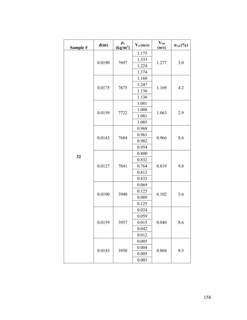
158
Sample # d(m)
𝜌s
(kg/m3) Vti (m/s)
Vtm
(m/s) 𝜎rel (%)
32
0.0190 7697
1.175
1.277 3.0 1.333
1.224
1.374
0.0175 7675
1.160
1.169 4.2 1.247
1.136
1.136
0.0159 7722
1.081
1.063 2.9 1.008
1.081
1.085
0.0143 7684
0.968
0.966 8.6 0.961
0.982
0.954
0.0127 7841
0.800
0.819 9.8
0.832
0.764
0.812
0.832
0.0190 3940
0.069
0.102 5.6 0.125
0.089
0.125
0.0159 3957
0.024
0.040 8.6
0.059
0.015
0.042
0.012
0.0143 3950
0.005
0.004 9.3 0.004
0.005
0.003
159
0
10
20
30
40
50
60
1.1 1.2 1.3 1.4 1.5
s (
%)
a

160
Appendix 4: MatLab codes for correlation development
Surface fitting for data points with 𝛼<1.3:
function [fitresult, gof] = createSurfaceFit1(alpha, TyTB, M_eq_M_N) alpha = alpha(:); TyTB = TyTB(:); M_eq_M_N = M_eq_M_N(:);
%% Fit: 'untitled fit 1'. ft = fittype( 'a*y^b*exp(x^c)+y^d+e', 'indep', {'x', 'y'}, 'depend',
'z' ); opts = fitoptions( ft ); opts.Display = 'Off'; opts.Lower = [-Inf -Inf -Inf -Inf -Inf]; opts.StartPoint = [0.521493347812023 0.944223846832328
0.305603466997734 0.143327062772478 0.548847435698431]; opts.Upper = [Inf Inf Inf Inf Inf]; opts.Weights = zeros(1,0); ex = excludedata( alpha, TyTB, 'Indices', [4 12 24 34 43 46 57 64 65
79 91 102] ); opts.Exclude = ex; [fitresult, gof] = fit( [alpha, TyTB], M_eq_M_N, ft, opts );
% Create a figure for the plots. figure( 'Name', 'untitled fit 1' );
% Plot fit with data. subplot( 2, 1, 1 ); h = plot( fitresult, [alpha, TyTB], M_eq_M_N, 'Exclude', ex ); legend( h, 'untitled fit 1', 'M_eq_M_N vs. alpha, TyTB', 'Excluded
M_eq_M_N vs. alpha, TyTB', 'Location', 'NorthEast' ); % Label axes xlabel( 'alpha' ); ylabel( 'TyTB' ); zlabel( 'M_eq_M_N' ); grid on view( 11.5, -10 );
% Plot residuals. subplot( 2, 1, 2 ); h = plot( fitresult, [alpha, TyTB], M_eq_M_N, 'Style', 'Residual',
'Exclude', ex ); legend( h, 'untitled fit 1 - residuals', 'Excluded M_eq_M_N vs.
alpha, TyTB', 'Location', 'NorthEast' ); % Label axes xlabel( 'alpha' ); ylabel( 'TyTB' ); zlabel( 'M_eq_M_N' ); grid on view( 26.5, 0 );
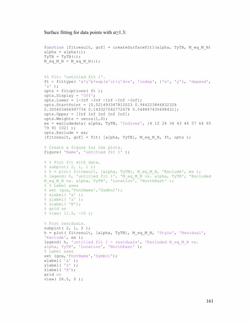
161
Surface fitting for data points with 𝛼≥1.3:
function [fitresult, gof] = createSurfaceFit1(alpha, TyTB, M_eq_M_N) alpha = alpha(:); TyTB = TyTB(:); M_eq_M_N = M_eq_M_N(:);
%% Fit: 'untitled fit 1'. ft = fittype( 'a*y^b*exp(x^c)+y^d+e', 'indep', {'x', 'y'}, 'depend',
'z' ); opts = fitoptions( ft ); opts.Display = 'Off'; opts.Lower = [-Inf -Inf -Inf -Inf -Inf]; opts.StartPoint = [0.521493347812023 0.944223846832328
0.305603466997734 0.143327062772478 0.548847435698431]; opts.Upper = [Inf Inf Inf Inf Inf]; opts.Weights = zeros(1,0); ex = excludedata( alpha, TyTB, 'Indices', [4 12 24 34 43 46 57 64 65
79 91 102] ); opts.Exclude = ex; [fitresult, gof] = fit( [alpha, TyTB], M_eq_M_N, ft, opts );
% Create a figure for the plots. figure( 'Name', 'untitled fit 1' );
% % Plot fit with data. % subplot( 2, 1, 1 ); % h = plot( fitresult, [alpha, TyTB], M_eq_M_N, 'Exclude', ex ); % legend( h, 'untitled fit 1', 'M_eq_M_N vs. alpha, TyTB', 'Excluded
M_eq_M_N vs. alpha, TyTB', 'Location', 'NorthEast' ); % % Label axes % set (gca,'FontName','Symbol'); % xlabel( 'a' ); % ylabel( 'z' ); % zlabel( 'B'); % grid on % view( 11.5, -10 );
% Plot residuals. subplot( 2, 1, 2 ); h = plot( fitresult, [alpha, TyTB], M_eq_M_N, 'Style', 'Residual',
'Exclude', ex ); legend( h, 'untitled fit 1 - residuals', 'Excluded M_eq_M_N vs.
alpha, TyTB', 'Location', 'NorthEast' ); % Label axes set (gca,'FontName','Symbol'); xlabel( 'a' ); ylabel( 'z' ); zlabel( 'B'); grid on view( 26.5, 0 );
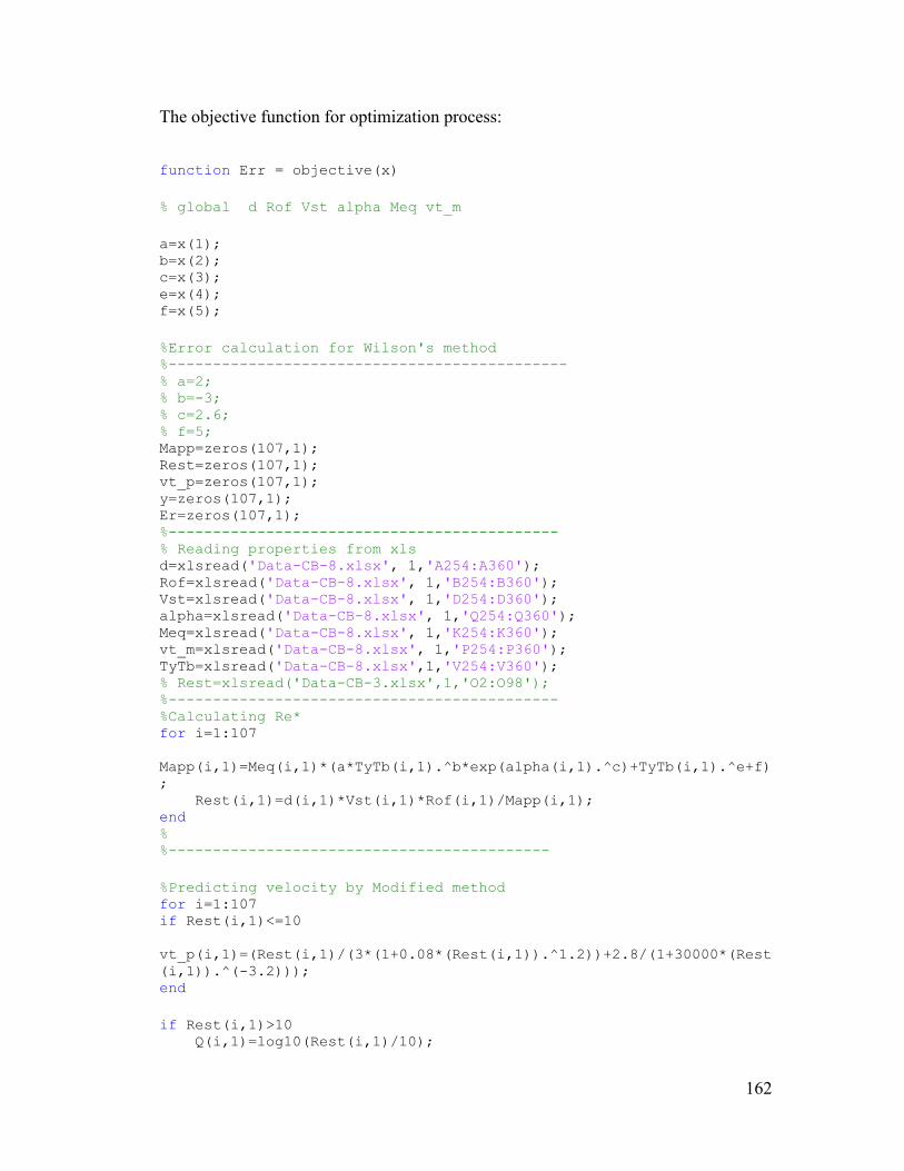
162
The objective function for optimization process:
function Err = objective(x)
% global d Rof Vst alpha Meq vt_m
a=x(1); b=x(2); c=x(3); e=x(4); f=x(5);
%Error calculation for Wilson's method %--------------------------------------------- % a=2; % b=-3; % c=2.6; % f=5; Mapp=zeros(107,1); Rest=zeros(107,1); vt_p=zeros(107,1); y=zeros(107,1); Er=zeros(107,1); %-------------------------------------------- % Reading properties from xls d=xlsread('Data-CB-8.xlsx', 1,'A254:A360'); Rof=xlsread('Data-CB-8.xlsx', 1,'B254:B360'); Vst=xlsread('Data-CB-8.xlsx', 1,'D254:D360'); alpha=xlsread('Data-CB-8.xlsx', 1,'Q254:Q360'); Meq=xlsread('Data-CB-8.xlsx', 1,'K254:K360'); vt_m=xlsread('Data-CB-8.xlsx', 1,'P254:P360'); TyTb=xlsread('Data-CB-8.xlsx',1,'V254:V360'); % Rest=xlsread('Data-CB-3.xlsx',1,'O2:O98'); %-------------------------------------------- %Calculating Re* for i=1:107
Mapp(i,1)=Meq(i,1)*(a*TyTb(i,1).^b*exp(alpha(i,1).^c)+TyTb(i,1).^e+f)
; Rest(i,1)=d(i,1)*Vst(i,1)*Rof(i,1)/Mapp(i,1); end % %-------------------------------------------
%Predicting velocity by Modified method for i=1:107 if Rest(i,1)<=10
vt_p(i,1)=(Rest(i,1)/(3*(1+0.08*(Rest(i,1)).^1.2))+2.8/(1+30000*(Rest
(i,1)).^(-3.2))); end
if Rest(i,1)>10 Q(i,1)=log10(Rest(i,1)/10);
163
y(i,1)=0.2069+0.5*Q(i,1)-0.158*(Q(i,1)).^1.72; vt_p(i,1)=(10.^(y(i,1))); end
if Rest(i,1)>=260 vt_p(i,1)=4.24; end end
%-------------------------------------------- %Calculating collective error for i=1:107 Er(i,1)=(vt_p(i,1)-vt_m(i,1)).^2; end Err=(mean(Er).^0.5);
164
Appendix 5: Genetic algorithm (GA)
Genetic algorithm is an optimization method used for solving both constrained and
unconstrained problems following the process of natural selection. The algorithm
generates several solutions in each iteration and selects individuals randomly from the
current generation and uses them as parents to produce children of the next
generation. A classic optimization algorithm generates a single point at each iteration
and the sequence of points reaches an optimum solution while GA generates a
population at each iteration and the best point at each population approaches an
optimal solution. The feature that makes GA a strong optimization method is that the
next population is always selected by computations which uses random number
generators. This feature avoids entrapment in local optimums and increases the
probability of reaching for the global optimum solution.
The following outline summarizes how the genetic algorithm works*:
1. The algorithm begins by creating a random initial population.
2. The algorithm then creates a sequence of new populations. At each step, the
algorithm uses the individuals in the current generation to create the next
population. To create the new population, the algorithm performs the following
steps:
a. Scores each member of the current population by computing its fitness
value.
b. Scales the raw fitness scores to convert them into a more usable range of
values.
c. Selects members, called parents, based on their fitness.
165
d. Some of the individuals in the current population that have lower fitness
are chosen as elite. These elite individuals are passed to the next
population.
e. Produces children from the parents. Children are produced either by
making random changes to a single parent—mutation—or by combining
the vector entries of a pair of parents—crossover.
f. Replaces the current population with the children to form the next
generation.
3. The algorithm stops when one of the stopping criteria is met.
* Mathworks. (2010). GA Optimization Toolbox: User's Guide (r2010a). Retrieved
March 5, 2015 from www.mathworks.com/help/pdf_doc/gads/gads_tb.pdf
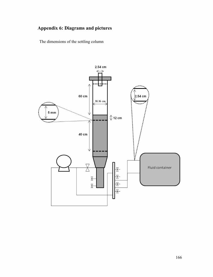
166
Appendix 6: Diagrams and pictures
The dimensions of the settling column
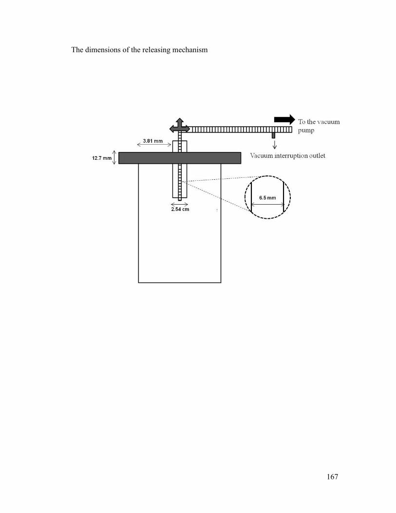
167
The dimensions of the releasing mechanism
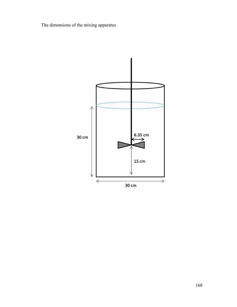
168
The dimensions of the mixing apparatus
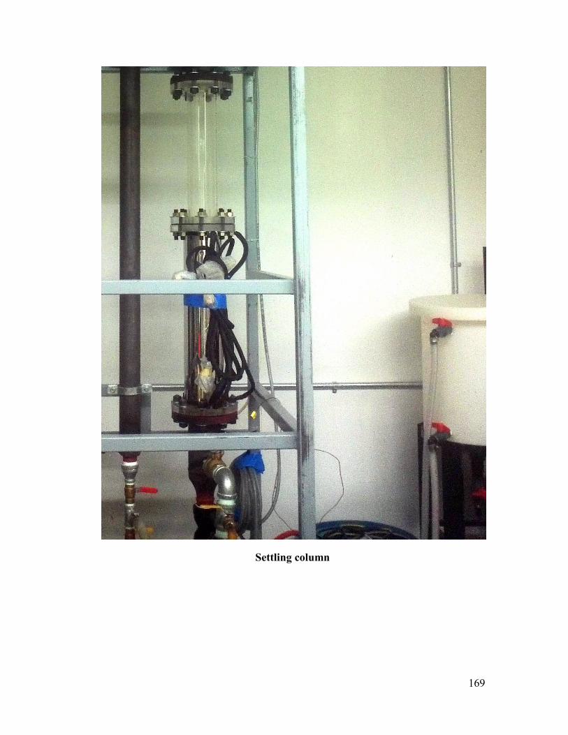
169
Settling column
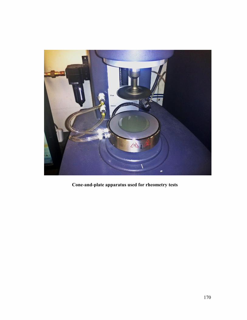
170
Cone-and-plate apparatus used for rheometry tests