Master of Science Thesis TU Delft, November 2017 Matteo

2

Master of Science Thesis TU Delft, November 2017 Matteo Baudino Bessone

3


Wave-structure interaction study, in the context of floating wind turbines, by mean of coupled rigid body

code and Fluidity CFD software

By

Matteo Baudino Bessone

in partial fulfilment of the requirements for the degree of

Master of Science

in Sustainable Energy Technology

at the Delft University of Technology, to be defended publicly on Thursday November 30, 2017 at 9:30 AM.

Supervisors: Dr. ir. A.C. Viré TU Delft MScEng. J.D. Brandsen TU Delft Thesis committee: Dr.-Ing. R. Schmehl TU Delft Dr. ir. A.C. Viré TU Delft

Dr.ir. A. J. Laguna TU Delft MScEng. J.D. Brandsen TU Delft

Cover picture from Offshore Wind Industry, www.offshorewindindustry.com, 2015

An electronic version of this thesis is available at http://repository.tudelft.nl/.

http://www.offshorewindindustry.com/

http://repository.tudelft.nl/

4


5


Dedication

To my family

6


7


Contents

Abstract ............................................................................................................................................................. 8 Acknowledgements ......................................................................................................................................... 9

List of figures .................................................................................................................................................. 10 List of tables ................................................................................................................................................... 12

List of symbols ............................................................................................................................................... 13

1. Introduction ............................................................................................................................................. 17 2. Theoretical background ......................................................................................................................... 20

2.1. Floating wind turbines ........................................................................................................................ 20

2.1.1. Classifications of the support structures for floating wind turbines ......................................... 20

2.1.2. Station keeping and connection cables....................................................................................... 22

2.1.3. The wind turbine ............................................................................................................................. 23 2.2. Wave theories ..................................................................................................................................... 25

2.2.1. Potential wave theory ..................................................................................................................... 25 2.2.2. Airy wave theory ............................................................................................................................. 27

2.3. Hydromechanics of floating rigid bodies ......................................................................................... 31 2.3.1. Hydrostatic analysis ....................................................................................................................... 31

2.3.2. Waves forces ................................................................................................................................... 32

2.3.3. Motions of a floating rigid body under the action of a regular wave train .............................. 35 3. Numerical Background .......................................................................................................................... 40

3.1. Governing Equations and discretisation ......................................................................................... 40 3.1.1. The Navier-Stokes equations ....................................................................................................... 40

3.1.2. The discretisation method ............................................................................................................. 41 3.2. The fluidity P1DG-P2 set-up ............................................................................................................... 45

3.3. The fluidity P0-P1CV set-up ............................................................................................................... 46 3.4. The immersed-body method for fluid-structure interaction .......................................................... 48

4. The Python code .................................................................................................................................... 50

4.1. The rigid body code ............................................................................................................................ 50

4.2. The fluid-structure interaction algorithm ......................................................................................... 55

4.3. The pressure integration ................................................................................................................... 57

5. Numerical experiments and discussion of results ............................................................................. 60

5.1. Propagation of linear waves in P1DG-P2 set-up ............................................................................. 60 5.2. Wave interaction with fixed body, P1DG-P2 set-up ........................................................................ 64 5.3. Propagation of linear waves in P0-P1CV set-up ............................................................................. 69

5.4. Wave interaction with heaving body, P0-P1CV set-up................................................................... 76 5.5. Wave interaction with freely-floating body, P0-P1CV set-up......................................................... 80

6. Conclusions and recommendations .................................................................................................... 84 6.1. Conclusions ......................................................................................................................................... 84

6.2. Recommendations ............................................................................................................................. 86

Appendix 1: linear waves formulations ...................................................................................................... 87 Appendix 2: discrete momentum equations .............................................................................................. 89

Bibliography .................................................................................................................................................... 92

8


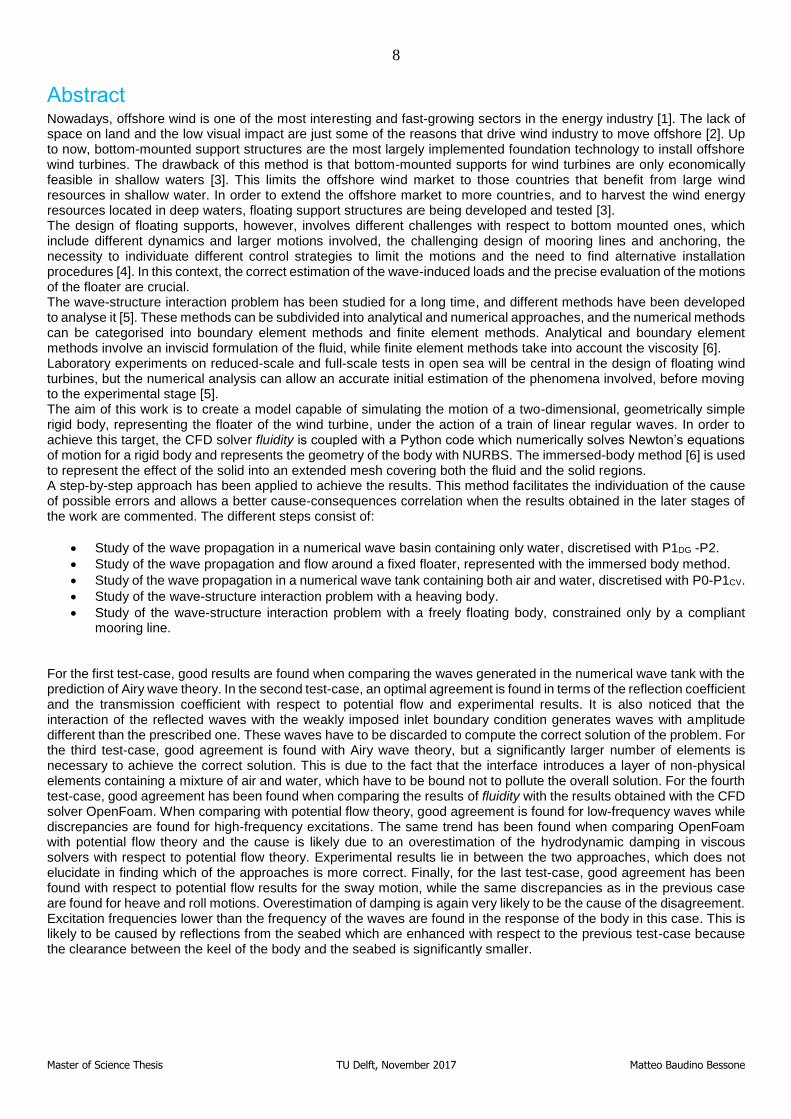
Abstract Nowadays, offshore wind is one of the most interesting and fast-growing sectors in the energy industry [1]. The lack of space on land and the low visual impact are just some of the reasons that drive wind industry to move offshore [2]. Up to now, bottom-mounted support structures are the most largely implemented foundation technology to install offshore wind turbines. The drawback of this method is that bottom-mounted supports for wind turbines are only economically feasible in shallow waters [3]. This limits the offshore wind market to those countries that benefit from large wind resources in shallow water. In order to extend the offshore market to more countries, and to harvest the wind energy resources located in deep waters, floating support structures are being developed and tested [3]. The design of floating supports, however, involves different challenges with respect to bottom mounted ones, which include different dynamics and larger motions involved, the challenging design of mooring lines and anchoring, the necessity to individuate different control strategies to limit the motions and the need to find alternative installation procedures [4]. In this context, the correct estimation of the wave-induced loads and the precise evaluation of the motions of the floater are crucial. The wave-structure interaction problem has been studied for a long time, and different methods have been developed to analyse it [5]. These methods can be subdivided into analytical and numerical approaches, and the numerical methods can be categorised into boundary element methods and finite element methods. Analytical and boundary element methods involve an inviscid formulation of the fluid, while finite element methods take into account the viscosity [6]. Laboratory experiments on reduced-scale and full-scale tests in open sea will be central in the design of floating wind turbines, but the numerical analysis can allow an accurate initial estimation of the phenomena involved, before moving to the experimental stage [5]. The aim of this work is to create a model capable of simulating the motion of a two-dimensional, geometrically simple rigid body, representing the floater of the wind turbine, under the action of a train of linear regular waves. In order to achieve this target, the CFD solver fluidity is coupled with a Python code which numerically solves Newton’s equations of motion for a rigid body and represents the geometry of the body with NURBS. The immersed-body method [6] is used to represent the effect of the solid into an extended mesh covering both the fluid and the solid regions. A step-by-step approach has been applied to achieve the results. This method facilitates the individuation of the cause of possible errors and allows a better cause-consequences correlation when the results obtained in the later stages of the work are commented. The different steps consist of:

• Study of the wave propagation in a numerical wave basin containing only water, discretised with P1DG -P2.

• Study of the wave propagation and flow around a fixed floater, represented with the immersed body method.

• Study of the wave propagation in a numerical wave tank containing both air and water, discretised with P0-P1CV.

• Study of the wave-structure interaction problem with a heaving body.

• Study of the wave-structure interaction problem with a freely floating body, constrained only by a compliant mooring line.

For the first test-case, good results are found when comparing the waves generated in the numerical wave tank with the prediction of Airy wave theory. In the second test-case, an optimal agreement is found in terms of the reflection coefficient and the transmission coefficient with respect to potential flow and experimental results. It is also noticed that the interaction of the reflected waves with the weakly imposed inlet boundary condition generates waves with amplitude different than the prescribed one. These waves have to be discarded to compute the correct solution of the problem. For the third test-case, good agreement is found with Airy wave theory, but a significantly larger number of elements is necessary to achieve the correct solution. This is due to the fact that the interface introduces a layer of non-physical elements containing a mixture of air and water, which have to be bound not to pollute the overall solution. For the fourth test-case, good agreement has been found when comparing the results of fluidity with the results obtained with the CFD solver OpenFoam. When comparing with potential flow theory, good agreement is found for low-frequency waves while discrepancies are found for high-frequency excitations. The same trend has been found when comparing OpenFoam with potential flow theory and the cause is likely due to an overestimation of the hydrodynamic damping in viscous solvers with respect to potential flow theory. Experimental results lie in between the two approaches, which does not elucidate in finding which of the approaches is more correct. Finally, for the last test-case, good agreement has been found with respect to potential flow results for the sway motion, while the same discrepancies as in the previous case are found for heave and roll motions. Overestimation of damping is again very likely to be the cause of the disagreement. Excitation frequencies lower than the frequency of the waves are found in the response of the body in this case. This is likely to be caused by reflections from the seabed which are enhanced with respect to the previous test-case because the clearance between the keel of the body and the seabed is significantly smaller.

9


Acknowledgements Very often writers of novel books say that acknowledgements are the most difficult part of their job. I used to think this was an exaggeration but, effectively, shrinking two years of life and work in half-a-page is challenging. Maybe not the toughest task ever, but still difficult. Therefore, I am writhing the acknowledgements right away, without thinking too much, but I hope I will still find the right words for all the people that have contributed to make these two years in Delft wonderful. First, I would thank my daily supervisor, Dr.Ir. Axelle Viré. She was always able to kindly point me in the right direction and motivate me with the right words. Also, I would thank her for her extremely valuable advice and for her helpfulness, which I think was much more extended than what MSc supervisors usually do. Then, I would thank my phd. supervisor, MScEng. Jaco Brandsen, for his helpfulness, that he extended far beyond the usual meeting hours, for his extremely useful advice and for the passion and dedication he showed to the subject, which was an example for me during this year. I would also thank the committee members, Dr.-Ing. Roland Schmehl and Dr.ir. Antonio Jarquin Laguna, for showing interest in the topic of this thesis and accepting to attend my presentation and defense. Subsequently, I would thank all the SET and Wind Energy students that made my studying here much more fun. Thanks to Andres, Andres, Bas, Ben, Clara, Greeshma, Irene, Ivan, Joe, Julia, Maarten, Marco, Marcos, Pranav, Roberto and Shajid. Also, I would thank my group of Italian friends in Delft, Alessandro, Antonio, Camilla, Davide, Edoardo, Federica, Federico, Francesco, Giulia, Greta, Luigi, Luca, Luca, Lucrezia, Matteo, Simone, Simone, Umberto, because they have never made me feel homesick. A special thank also to my friends back in Turin, because they pushed me to keep working to come to Delft, also when it seemed I was not to make it and I was giving up. Last but definitely not the least, the biggest thank goes to my family, since they supported my decision to come in the Netherlands and encouraged me in all the possible ways. All I have achieved in these years is thanks to you.

10


List of figures

Figure 1.1: Growth in offshore wind capacity 2011-2016 [1] .................................................................. 17

Figure 1.2: Offshore wind resources in Europe [7] .................................................................................. 17

Figure 1.3: Wind turbine support concepts with increasing water depth [8] ........................................ 18 Figure 2.1.1.1: Different substructure concepts for floating wind turbines [16]. .................................. 21 Figure 2.1.2.1: Floating offshore wind turbine system for spar buoy design [3]................................. 23

Figure 2.1.3.1: Floating HAWT [54] ............................................................................................................ 24 Figure 2.1.3.2: Floating VAWT [55] ............................................................................................................ 24

Figure 2.2.2.1: Orbits of deep waters particles [26] ................................................................................. 29 Figure 2.2.2.2: Orbits of shallow waters particles [26] ............................................................................. 29

Figure 2.2.2.3: Regions of validity of various wave theories [23] .......................................................... 30

Figure 2.3.1.1: Stability of a nearly rectangular body [21] ...................................................................... 32 Figure 2.3.2.1: Loading regimes for vertical circular cylinders [21] ....................................................... 34

Figure 2.3.2.2: Scattered waves generated by the interaction of a train of regular waves with a large structure [27] ........................................................................................................................................ 35 Figure 2.3.3.1: Degrees of freedom for floating wind turbine [28] ......................................................... 35

Figure 2.3.3.2: RAO and phase-shift as a function of wave frequency [26] ........................................ 37

Figure 2.3.3.3: Frequency regions and motion behaviour [26] .............................................................. 38

Figure 3.1.2.1: Piecewise linear (a, c) and piecewise quadratic (b, d) continuous shape functions for one-dimensional and two-dimensional problems [33], [34] ............................................................... 42

Figure 3.1.2.2: Piecewise linear (a, c) and piecewise quadratic (b, d) discontinuous shape functions for one-dimensional and two-dimensional problems [33], [34] ............................................. 43 Figure 3.1.2.3: One-dimensional and two-dimensional shape function for finite volume discretisation [33], [34] .................................................................................................................................. 44

Figure 3.1.2.4: Comparison between (a) a classic finite volume mesh and (b) a control volume mesh obtained from a piecewise linear finite element mesh (dashed lines) [33], [34] ....................... 44

Figure 4.1.1: Convex hulls for linear and quadratic curves [41]............................................................. 52

Figure 4.1.2: motion computed with RBC versus predicted motion ...................................................... 54

Figure 4.1.3: Phase-shift computed with RBC versus predicted phase-shift ....................................... 54

Figure 4.2.1: Schematic representation of the relation between the different codes adopted .......... 55 Figure 4.2.2: Wave-structure interaction algorithm, Δt0 pre-timestep, Δt1 first timestep, Δtn n timestep ........................................................................................................................................................... 56

Figure 4.3.1: Intersection of shell side with mesh elements ................................................................... 57

Figure 4.3.2: Convergence of the hydrostatic force on: coarse grid - dot-dashed black; intermediate grid - blue dashed; fine grid - red dashed; theoretical prediction - green dashed ............................... 59

Figure 5.1.1: Geometrical sketch of the two-dimensional numerical wave tank. WL stands for wavelength ..................................................................................................................................................... 60

Figure 5.1.2: Free surface elevation at a) 𝒙/𝝀 = 0.2 and b) 𝒙/𝝀 = 0.4 ................................................. 62

Figure 5.1.3: Horizontal water particles velocity at 𝒙/ 𝝀 = 0.2 and 𝒙/𝝀 = 0.4 ...................................... 62

Figure 5.1.4: Free surface elevation, t/T=16 ............................................................................................. 62

Figure 5.1.5: Velocity profile, t/T=16 .......................................................................................................... 63

Figure 5.1.6: Fourier transform of steady-state wave propagation, 𝒙/𝝀 = 0.2 ..................................... 63

Figure 5.2.1: Geometrical sketch of the two-dimensional numerical wave tank with fixed body. WL stands for wavelength ................................................................................................................................... 64

Figure 5.2.2: Velocity profile, t/T =16 ......................................................................................................... 65

Figure 5.2.3: Transmission coefficients obtained by simulations with fluidity – red dots, compared with experimental – green squares and theoretical - blue triangles - results [45] ............................... 66

Figure 5.2.4: Reflection coefficients obtained by simulations with fluidity – red dots, compared with experimental – green squares and theoretical - blue triangles - results [45] ....................................... 66

11


Figure 5.2.5: Time series of wave amplitude recorded at the wave maker, 𝒙/𝝀 =0 ........................... 67

Figure 5.2.6: Transmission coefficients obtained by simulations with fluidity, – red dots, taking into account the waves not polluted by the reflection to the wavemaker, compared with experimental – green squares and theoretical - blue triangles results [45] ..................................................................... 67 Figure 5.2.7: Reflection coefficients obtained by simulations with fluidity, – red dots, taking into account the waves not polluted by the reflection to the wavemaker, compared with experimental – green squares and theoretical - blue triangles results [45] ..................................................................... 68

Figure 5.3.1: Representation of the mesh ................................................................................................. 69

Figure 5.3.2: Geometrical sketch of the two-dimensional numerical wave tank. WL stands for wavelength ..................................................................................................................................................... 70 Figure 5.3.3: Water particles non-dimensional velocity profile, t/T=8, without material volume fraction ............................................................................................................................................................. 71

Figure 5.3.4: Water particles non-dimensional velocity profile, t/T=8, with material volume fraction .......................................................................................................................................................................... 71

Figure 5.3.5: Time series of waves induced pressure at 𝒙/𝝀 =1 (a, c) and at 𝒙/𝝀 =2 (b, d). The recording gauges are placed at 0.01 m depth (a, b) and at 0.2 m depth (c, d). Green dashed - coarse mesh, black dot - intermediate mesh, blue dashed - refined mesh ......................................... 72

Figure 5.3.6: Time series of horizontal water particles velocity at 𝒙/𝝀 =1 (a, c) and at 𝒙/𝝀 =2 (b, d). The recording gauges are 0.01 m depth (a, b) and at 0.2 m depth (c, d). Green dashed coarse mesh, black dot-intermediate mesh, blue dashed refined mesh ........................................................... 72 Figure 5.3.7: Geometrical sketch of the scaled-down two-dimensional numerical wave tank. WL stands for wavelength ................................................................................................................................... 73

Figure 5.3.8: Time series of waves induced pressure at 𝒙/𝝀 =0.8 (a, c) and at 𝒙/𝝀 =1.7 (b, d). The recording gauges are placed at 0.001 m depth (a, b) and at 0.005 m depth (c, d) ............................ 74

Figure 5.3.9: Time series of horizontal water particles velocity at 𝒙/𝝀 =0.8 (a, c) and at 𝒙/𝝀 =1.7 (b, d). The recording gauges are placed at 0.001 m depth (a, b) and at 0.005 m depth (c, d)............... 74

Figure 5.4.1: Geometrical sketch of the two-dimensional numerical wave tank with heaving body. WL stands for wavelength ............................................................................................................................ 77 Figure 5.4.2: Mesh convergence study ...................................................................................................... 77

Figure 5.4.3: Non-dimensional heave motion for set of waves 4, red solid line – fluidity; blue dashed line – OpenFoam; black dash-dotted line – potential flow [51] ................................................ 78 Figure 5.4.4: RAO, red circles - fluidity; green squares – experimental [31]; blue triangles - potential flow; black hexagons - OpenFoam [51] ..................................................................................... 78 Figure 5.4.5: Added mass a) and hydrodynamic damping b) computed with different approaches [51] ................................................................................................................................................................... 79

Figure 5.5.1: Geometrical sketch of the two-dimensional numerical wave tank with rotating body. WL stands for wavelength ............................................................................................................................ 80

Figure 5.5.2: Heave motion computed by fluidity - solid red line, against potential flow predicted heave amplitude – blue dashed line ........................................................................................................... 81

Figure 5.5.3: Roll motion computed by fluidity - solid red line, against potential flow predicted roll amplitude – blue dashed line ....................................................................................................................... 81 Figure 5.5.4: Sway motion computed by fluidity - solid red line, against potential flow predicted sway amplitude – blue dashed line ............................................................................................................. 81

Figure 5.5.5: Roll a) and sway c) added mass and hydrodynamic damping b),d) with different approaches [51] ............................................................................................................................................. 82

12


List of tables

Table 2.1.1.1: Qualitative assessment of different floating support designs [3], [15] ......................... 22

Table 4.3.1: Mesh parameters for hydrostatic validation pressure integration .................................... 58

Table 5.1.1: Waves parameters waves propagation P1DG-P2 ............................................................... 61 Table 5.1.2: Mesh parameters waves propagation P1DG-P2 ................................................................. 61 Table 5.2.1: Waves parameters fixed body P1DG-P2 .............................................................................. 65

Table 5.2.2: Mesh parameters fixed body P1DG-P2 ................................................................................. 65 Table 5.3.1: Waves parameters waves propagation P0-P1CV ............................................................... 70

Table 5.3.2: Mesh parameters waves propagation P0-P1CV .................................................................. 70 Table 5.3.3: Waves parameters waves propagation P0-P1CV ............................................................... 73

Table 5.3.4: Mesh parameters waves propagation P0-P1CV, scaled down ......................................... 73

Table 5.4.1: Waves parameters heaving body P0-P1CV ......................................................................... 76 Table 5.4.2: Mesh parameters heaving body P0-P1CV ........................................................................... 77

Table 5.5.1: Waves parameters rotating body P0-P1CV .......................................................................... 80 Table 5.5.2: Mesh parameters rotating body P0-P1CV ............................................................................ 80

Table 5.5.3: Amplitude of motions computed in fluidity against amplitude of motions computed by potential flow .................................................................................................................................................. 82

13


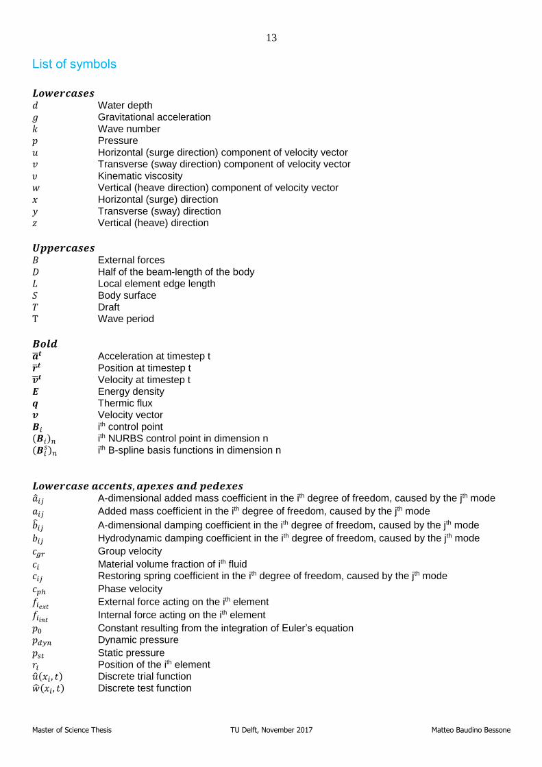
List of symbols

𝑳𝒐𝒘𝒆𝒓𝒄𝒂𝒔𝒆𝒔 𝑑 Water depth 𝑔 Gravitational acceleration

𝑘 Wave number 𝑝 Pressure

𝑢 Horizontal (surge direction) component of velocity vector 𝑣 Transverse (sway direction) component of velocity vector

𝜐 Kinematic viscosity 𝑤 Vertical (heave direction) component of velocity vector

𝑥 Horizontal (surge) direction 𝑦 Transverse (sway) direction 𝑧 Vertical (heave) direction

𝑼𝒑𝒑𝒆𝒓𝒄𝒂𝒔𝒆𝒔 𝐵 External forces

𝐷 Half of the beam-length of the body 𝐿 Local element edge length

𝑆 Body surface 𝑇 Draft T Wave period

𝑩𝒐𝒍𝒅 �̅�𝒕 Acceleration at timestep t

�̅�𝒕 Position at timestep t

�̅�𝒕 Velocity at timestep t 𝑬 Energy density 𝒒 Thermic flux 𝒗 Velocity vector

𝑩𝑖 ith control point (𝑩𝑖)𝑛 ith NURBS control point in dimension n (𝑩𝑖

𝑠)𝑛 ith B-spline basis functions in dimension n

𝑳𝒐𝒘𝒆𝒓𝒄𝒂𝒔𝒆 𝒂𝒄𝒄𝒆𝒏𝒕𝒔, 𝒂𝒑𝒆𝒙𝒆𝒔 𝒂𝒏𝒅 𝒑𝒆𝒅𝒆𝒙𝒆𝒔 �̂�𝑖𝑗 A-dimensional added mass coefficient in the ith degree of freedom, caused by the jth mode

𝑎𝑖𝑗 Added mass coefficient in the ith degree of freedom, caused by the jth mode

�̂�𝑖𝑗 A-dimensional damping coefficient in the ith degree of freedom, caused by the jth mode

𝑏𝑖𝑗 Hydrodynamic damping coefficient in the ith degree of freedom, caused by the jth mode

𝑐𝑔𝑟 Group velocity

𝑐𝑖 Material volume fraction of ith fluid 𝑐𝑖𝑗 Restoring spring coefficient in the ith degree of freedom, caused by the jth mode

𝑐𝑝ℎ Phase velocity

𝑓𝑖𝑒𝑥𝑡 External force acting on the ith element

𝑓𝑖𝑖𝑛𝑡 Internal force acting on the ith element

𝑝0 Constant resulting from the integration of Euler’s equation 𝑝𝑑𝑦𝑛 Dynamic pressure

𝑝𝑠𝑡 Static pressure 𝑟𝑖 Position of the ith element

�̂�(𝑥𝑖, 𝑡) Discrete trial function �̂�(𝑥𝑖, 𝑡) Discrete test function

14


Δ𝑡 Timestep size

15


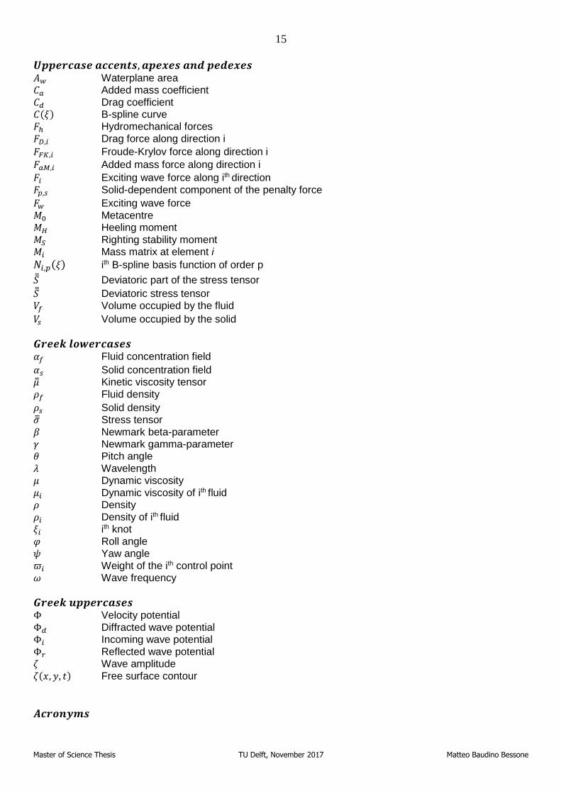
𝑼𝒑𝒑𝒆𝒓𝒄𝒂𝒔𝒆 𝒂𝒄𝒄𝒆𝒏𝒕𝒔, 𝒂𝒑𝒆𝒙𝒆𝒔 𝒂𝒏𝒅 𝒑𝒆𝒅𝒆𝒙𝒆𝒔

𝐴𝑤 Waterplane area 𝐶𝑎 Added mass coefficient

𝐶𝑑 Drag coefficient 𝐶(𝜉) B-spline curve 𝐹ℎ Hydromechanical forces

𝐹𝐷,𝑖 Drag force along direction i

𝐹𝐹𝐾,𝑖 Froude-Krylov force along direction i 𝐹𝑎𝑀,𝑖 Added mass force along direction i 𝐹𝑖 Exciting wave force along ith direction

𝐹𝑝,𝑠 Solid-dependent component of the penalty force

𝐹𝑤 Exciting wave force

𝑀0 Metacentre 𝑀𝐻 Heeling moment 𝑀𝑆 Righting stability moment 𝑀𝑖 Mass matrix at element i

𝑁𝑖,𝑝(𝜉) ith B-spline basis function of order p

𝑆̿ Deviatoric part of the stress tensor

𝑆̿ Deviatoric stress tensor 𝑉𝑓 Volume occupied by the fluid

𝑉𝑠 Volume occupied by the solid

𝑮𝒓𝒆𝒆𝒌 𝒍𝒐𝒘𝒆𝒓𝒄𝒂𝒔𝒆𝒔 𝛼𝑓 Fluid concentration field

𝛼𝑠 Solid concentration field �̿� Kinetic viscosity tensor

𝜌𝑓 Fluid density

𝜌𝑠 Solid density �̿� Stress tensor

𝛽 Newmark beta-parameter 𝛾 Newmark gamma-parameter 𝜃 Pitch angle

𝜆 Wavelength 𝜇 Dynamic viscosity

𝜇𝑖 Dynamic viscosity of ith fluid 𝜌 Density

𝜌𝑖 Density of ith fluid 𝜉𝑖 ith knot

𝜑 Roll angle 𝜓 Yaw angle

𝜛𝑖 Weight of the ith control point 𝜔 Wave frequency

𝑮𝒓𝒆𝒆𝒌 𝒖𝒑𝒑𝒆𝒓𝒄𝒂𝒔𝒆𝒔 Φ Velocity potential

Φ𝑑 Diffracted wave potential Φ𝑖 Incoming wave potential

Φ𝑟 Reflected wave potential 𝜁 Wave amplitude

𝜁(𝑥, 𝑦, 𝑡) Free surface contour

𝑨𝒄𝒓𝒐𝒏𝒚𝒎𝒔

16


𝐵𝐸𝑀 Boundary element method

𝐵 − 𝑆𝑝𝑙𝑖𝑛𝑒 Basis Spline 𝐶𝐺 Continuous Galerkin

𝐷𝐺 Discontinuous Galerkin 𝐹𝐸𝐴 Finite element analysis

𝐹𝐸𝑀 Finite element method 𝐹𝑉 Finite volumes

𝐻𝐴𝑊𝑇 Horizontal axis wind turbine 𝑁𝑈𝑅𝐵𝑆 Non-Uniform Rational Basis-Splines

𝑃𝑃 Points per 𝑅𝐴𝑂 Response amplitude operator

𝑅𝐵𝐶 Rigid body code 𝑇𝐿𝑃 Tension leg platform 𝑉𝐴𝑊𝑇 Vertical axis wind turbine

17


1. Introduction

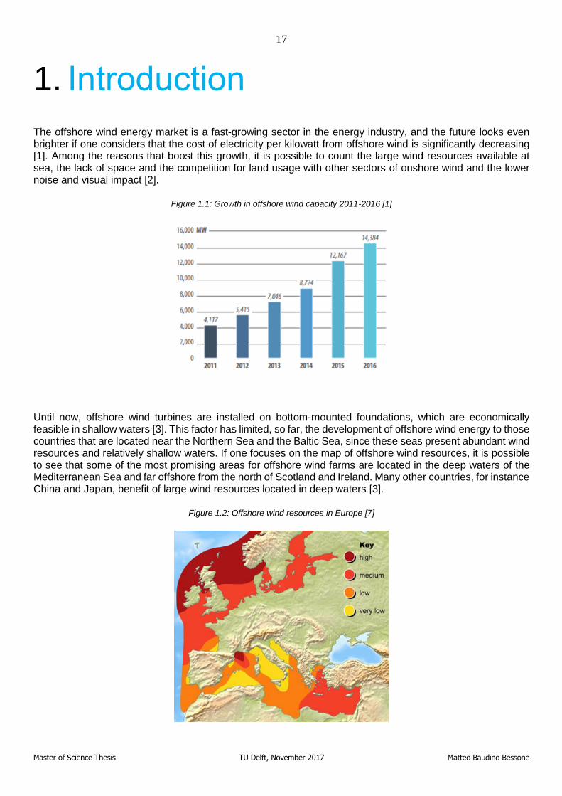
The offshore wind energy market is a fast-growing sector in the energy industry, and the future looks even brighter if one considers that the cost of electricity per kilowatt from offshore wind is significantly decreasing [1]. Among the reasons that boost this growth, it is possible to count the large wind resources available at sea, the lack of space and the competition for land usage with other sectors of onshore wind and the lower noise and visual impact [2].

Figure 1.1: Growth in offshore wind capacity 2011-2016 [1]

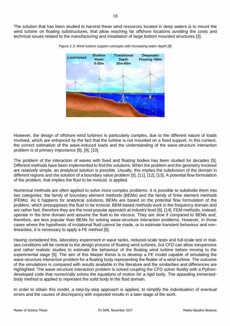
Until now, offshore wind turbines are installed on bottom-mounted foundations, which are economically feasible in shallow waters [3]. This factor has limited, so far, the development of offshore wind energy to those countries that are located near the Northern Sea and the Baltic Sea, since these seas present abundant wind resources and relatively shallow waters. If one focuses on the map of offshore wind resources, it is possible to see that some of the most promising areas for offshore wind farms are located in the deep waters of the Mediterranean Sea and far offshore from the north of Scotland and Ireland. Many other countries, for instance China and Japan, benefit of large wind resources located in deep waters [3].

Figure 1.2: Offshore wind resources in Europe [7]

18


The solution that has been studied to harvest these wind resources located in deep waters is to mount the wind turbine on floating substructures, that allow reaching far offshore locations avoiding the costs and technical issues related to the manufacturing and installation of large bottom mounted structures [3].

Figure 1.3: Wind turbine support concepts with increasing water depth [8]

However, the design of offshore wind turbines is particularly complex, due to the different nature of loads involved, which are enhanced by the fact that the turbine is not mounted on a fixed support. In this context, the correct estimation of the wave-induced loads and the understanding of the wave-structure interaction problem is of primary importance [6], [9], [10].

The problem of the interaction of waves with fixed and floating bodies has been studied for decades [5]. Different methods have been implemented to find the solutions. When the problem and the geometry involved are relatively simple, an analytical solution is possible. Usually, this implies the subdivision of the domain in different regions and the solution of a boundary value problem [5], [11], [12], [13]. A potential flow formulation of the problem, that implies the fluid to be inviscid, is applied.

Numerical methods are often applied to solve more complex problems. It is possible to subdivide them into two categories: the family of boundary element methods (BEMs) and the family of finite element methods (FEMs). As it happens for analytical solutions, BEMs are based on the potential flow formulation of the problem, which presupposes the fluid to be inviscid. BEM-based methods work in the frequency domain and are rather fast, therefore they are the most popular approach at industry level [6], [14]. FEM methods, instead, operate in the time domain and assume the fluid to be viscous. They are slow if compared to BEMs and, therefore, are less popular than BEMs for solving wave-structure interaction problems. However, in those cases where the hypothesis of irrotational fluid cannot be made, or to estimate transient behaviour and non-linearities, it is necessary to apply a FE method [6].

Having considered this, laboratory experiment in wave tanks, reduced-scale tests and full-scale test in real-sea conditions will be central to the design process of floating wind turbines, but CFD can allow inexpensive and rather realistic studies to estimate the behaviour of the floating wind turbine before moving to the experimental stage [5]. The aim of this Master thesis is to develop a FE model capable of simulating the wave-structure interaction problem for a floating body representing the floater of a wind turbine. The outcome of the simulations is compared with results available in the literature and the similarities and differences are highlighted. The wave-structure interaction problem is solved coupling the CFD solver fluidity with a Python-developed code that numerically solves the equations of motion for a rigid body. The appealing immersed-body method is applied to represent the solid body in the fluid domain.

In order to obtain this model, a step-by-step approach is applied, to simplify the individuation of eventual errors and the causes of discrepancy with expected results in a later stage of the work.

19


For each stage of the work, a research question is formulated, that has to be addressed.

• How accurate is the CFD prediction of waves’ propagation in a two-dimensional numerical wave tank containing only water and discretised with P1DG -P2, when compared to linear Airy wave theory?

• How precise is the CFD solution of the wave-structure interaction problem with a fixed body represented with the immersed-body method?

• How accurate is the CFD prediction of waves propagation in a two-dimensional numerical wave tank containing both air and water and discretised with P0-P1CV with respect to linear Airy wave theory? And which side effects are caused by the necessity to represent an air-water interface?

• For the wave-structure interaction problem for a heaving body represented with the immersed-body method, how close is the agreement between the results predicted in fluidity and the results obtained with other methods? And which phenomena can cause discrepancies?

• How precise is the CFD solution of a wave-structure interaction problem for the case of a freely floating body constrained only by a compliant mooring line? And which effects can be the cause of differences when fluidity results are compared to the results predicted with potential flow theory?

20


2. Theoretical background

In this section, a brief introduction to the typologies, components and main aspects of floating wind turbines is presented. Subsequently, the governing equations and boundary conditions of the potential wave theory are introduced, focusing on linear Airy wave theory. Finally, the dynamics of a two-dimensional rigid body under the action of a train of linear waves are reported.

2.1. Floating wind turbines

A floating wind turbine can be subdivided into three main sub-components: the floating substructure, the seakeeping, namely mooring lines and anchors, and the wind turbine. In this subchapter, the role of these three components is outlined and the main technological solutions available are compared.

2.1.1. Classifications of the support structures for floating wind turbines

The main structure, that consists of the platform and the floater, has mainly four roles [15]: hold the turbine into position, maintain the deflections in a range acceptable for the electrical cables, counteract the turbine induced loads and counterbalance the waves and current effort, transferring the loads from the structure to the dissipating medium. In the case of floating structures, the medium is the water, which comports two relevant advantages upon transferring the loads to the soil, as it happens in the case of bottom-mounted structures. First, water is closer, which means that the overturning moment lever arm would be shorter and, as a consequence, the moment exerted will be lower. Second, water is a compliant material, which can result in minor peak forces [15].

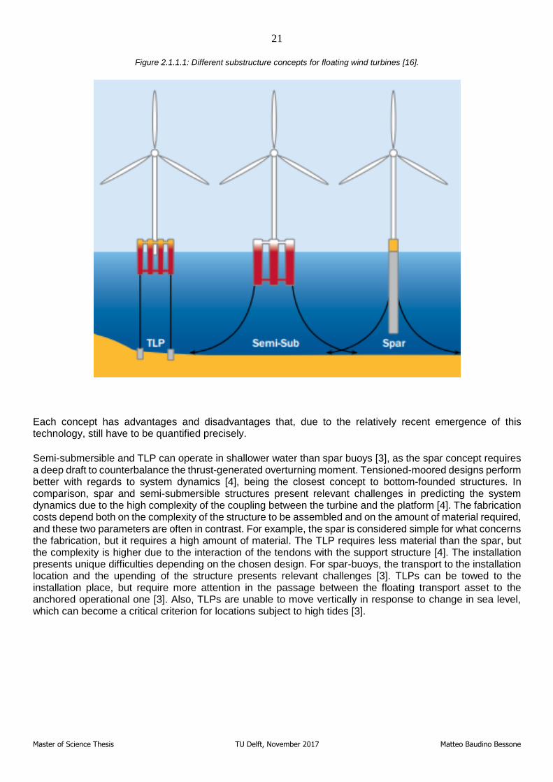
As it is the case for fixed structures, there exist different concepts for the floating substructure. These dissimilarities are mainly a consequence of how the foundation counterbalances the thrust force acting on the rotor and stabilises the whole structure [3]. According to this, floating support-structure are classified as follows:

• Spar structures that rely on gravity to counterweight the environmental loads

• Semi-submersible structures or barges that take advantage of distributed buoyancy

• Tensioned-moored or tension-leg platform (TLP) concepts relying on taut moorings to hold them in position

Effectively, each approach is a hybrid design that takes advantage of all the three previously mentioned mechanisms to stabilise the structure, but for each design, one is predominating [3]. Therefore, in the limiting case, the spar buoy can be considered a tank with zero waterplane area but with enough ballast below the sea surface to compensate the thrust-induced overturning moment. For the spar design, mooring lines do not play a critical role in the stability of the structure but are conceived to contrast the mean waves drift force, avoiding the buoy to be drifted away. The TLP can be represented as a zero-weight basin with zero waterplane area, stabilised by the taut moorings, which fully constrain vertical motions. Finally, the barge can be represented as a zero-weight vessel that relies on the waterplane area for stabilisation and would rely on mooring lines only to avoid drifting [4].

21


Figure 2.1.1.1: Different substructure concepts for floating wind turbines [16].

Each concept has advantages and disadvantages that, due to the relatively recent emergence of this technology, still have to be quantified precisely.

Semi-submersible and TLP can operate in shallower water than spar buoys [3], as the spar concept requires a deep draft to counterbalance the thrust-generated overturning moment. Tensioned-moored designs perform better with regards to system dynamics [4], being the closest concept to bottom-founded structures. In comparison, spar and semi-submersible structures present relevant challenges in predicting the system dynamics due to the high complexity of the coupling between the turbine and the platform [4]. The fabrication costs depend both on the complexity of the structure to be assembled and on the amount of material required, and these two parameters are often in contrast. For example, the spar is considered simple for what concerns the fabrication, but it requires a high amount of material. The TLP requires less material than the spar, but the complexity is higher due to the interaction of the tendons with the support structure [4]. The installation presents unique difficulties depending on the chosen design. For spar-buoys, the transport to the installation location and the upending of the structure presents relevant challenges [3]. TLPs can be towed to the installation place, but require more attention in the passage between the floating transport asset to the anchored operational one [3]. Also, TLPs are unable to move vertically in response to change in sea level, which can become a critical criterion for locations subject to high tides [3].

22


Table 2.1.1.1: Qualitative assessment of different floating support designs [3], [15]

Spar buoy TLP Semi-submersible

Water depth Deeper Shallower Shallower

Stability Gravity Moorings Hydrostatics

Cost Uncertain (presumably

good) Uncertain Uncertain

Fabrication Potentially simple More complex More complex

Installation More complex More complex Good

2.1.2. Station keeping and connection cables

The other components that integrate the floating support are the mooring lines, the anchoring and the electricity cables. The mooring lines connect the floater to the seabed and provide the necessary restoring force to counteract the mean drift force. For TLP designs taut moorings have also to provide the required stability to the whole structure. The anchoring connects the mooring to the sea-bed. The connection cables export the electricity produced by the turbine to shore.

Mooring lines make it feasible to locate floating wind turbines in deep waters, where bottom-founded structures are not economically feasible [3], obviating to the construction of large and expensive towers [17]. The requirements for mooring lines are that they must withstand extreme loads, fatigue and be rigid enough to have natural frequency above the wave frequencies [3]. The mooring lines commonly consist of chains, wire ropes and synthetic fibre ropes or a combination of chains and ropes [18]. Chains have been used for a long time by offshore industry, and each chain relies on its weight to assure the necessary tension to the moored vessel [18]. Cathodic protections are often used to avoid corrosion [3]. The weight of each chain that holds each mooring line in tension introduces a major drawback. It induces a resultant force on the floater [18], which can become prohibitive with increasing water depth and chain length [3]. Therefore, neutrally buoyant synthetic fibres and hybrid systems have been tested, that allow the desired tension to be reached without adding excessive weight to the structure.

The design of the mooring lines can follow two different approaches: a quasi-static model and a dynamic model [3]. The difference relies in the capability of the dynamic model to capture higher peaks of tension and the interaction with the environment, which is absent in the quasi-static approach [3]. For the quasi-static approach two different options are viable: a linear spring system, which is valid in case of small displacements of the body and can be described by Hook’s law, and a freely hanging chain model, which solves the two non-linear equations of static equilibrium written as a function of the applied forces and the relative weight of the chain to obtain the anchor forces [3].The dynamic approach can be subdivided into a lumped-mass model, a finite element and a finite difference model. The mooring line is usually represented as a sequence of spring-damper systems, and the governing discretised equation that holds true for all of these approaches is [3]:

𝑀𝑖�̈�𝑖 =∑𝒇𝑖𝑒𝑥𝑡 +∑𝒇𝑖𝑖𝑛𝑡 , 2.1.2.1

where:

• 𝑀𝑖 is the mass matrix • 𝒓𝑖 position of the ith node • ∑𝒇𝑖𝑒𝑥𝑡 is the resultant of the external forces

• ∑𝒇𝑖𝑖𝑛𝑡 is the resultant of the internal forces

23


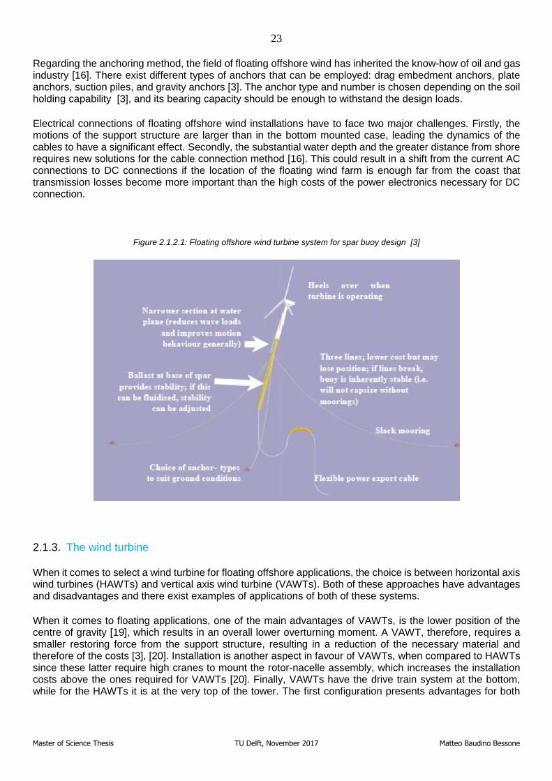
Regarding the anchoring method, the field of floating offshore wind has inherited the know-how of oil and gas industry [16]. There exist different types of anchors that can be employed: drag embedment anchors, plate anchors, suction piles, and gravity anchors [3]. The anchor type and number is chosen depending on the soil holding capability [3], and its bearing capacity should be enough to withstand the design loads.

Electrical connections of floating offshore wind installations have to face two major challenges. Firstly, the motions of the support structure are larger than in the bottom mounted case, leading the dynamics of the cables to have a significant effect. Secondly, the substantial water depth and the greater distance from shore requires new solutions for the cable connection method [16]. This could result in a shift from the current AC connections to DC connections if the location of the floating wind farm is enough far from the coast that transmission losses become more important than the high costs of the power electronics necessary for DC connection.

Figure 2.1.2.1: Floating offshore wind turbine system for spar buoy design [3]

2.1.3. The wind turbine

When it comes to select a wind turbine for floating offshore applications, the choice is between horizontal axis wind turbines (HAWTs) and vertical axis wind turbine (VAWTs). Both of these approaches have advantages and disadvantages and there exist examples of applications of both of these systems.

When it comes to floating applications, one of the main advantages of VAWTs, is the lower position of the centre of gravity [19], which results in an overall lower overturning moment. A VAWT, therefore, requires a smaller restoring force from the support structure, resulting in a reduction of the necessary material and therefore of the costs [3], [20]. Installation is another aspect in favour of VAWTs, when compared to HAWTs since these latter require high cranes to mount the rotor-nacelle assembly, which increases the installation costs above the ones required for VAWTs [20]. Finally, VAWTs have the drive train system at the bottom, while for the HAWTs it is at the very top of the tower. The first configuration presents advantages for both

24


what concerns the accessibility of the transmission and generation system, and the stability of the structure [19].

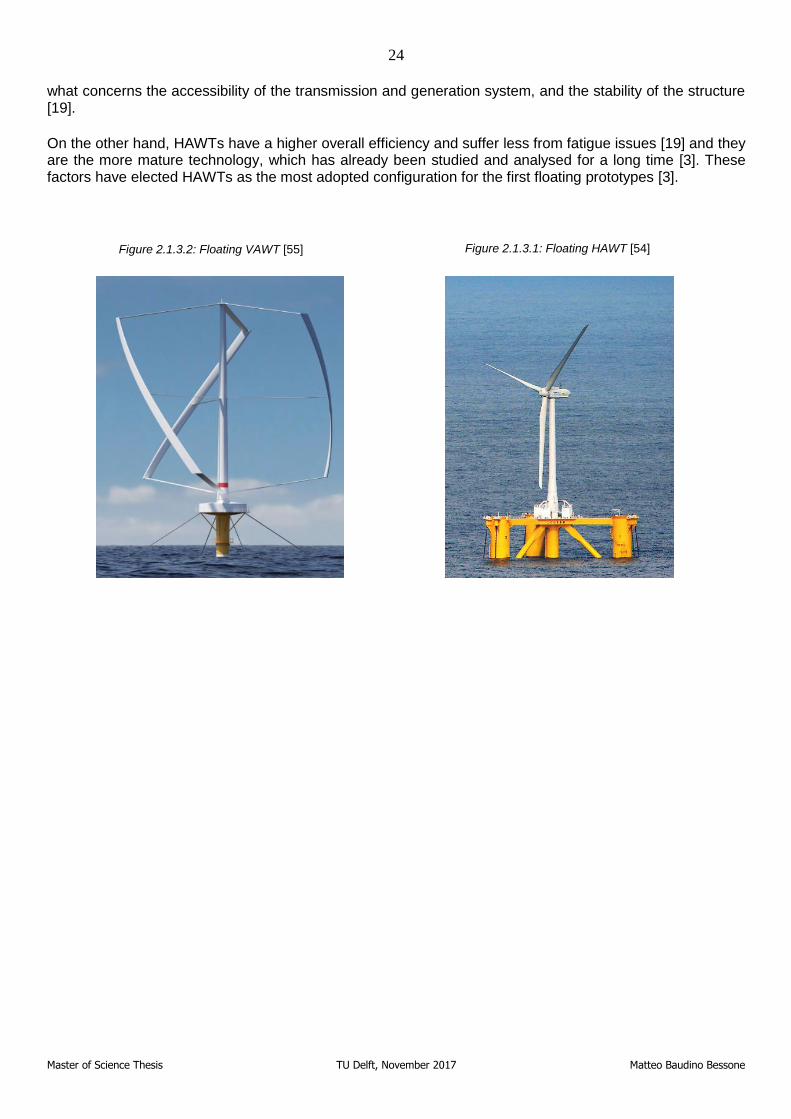
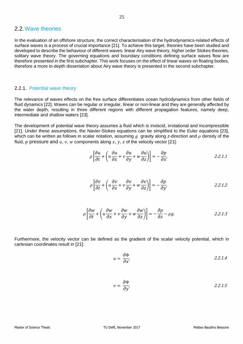
On the other hand, HAWTs have a higher overall efficiency and suffer less from fatigue issues [19] and they are the more mature technology, which has already been studied and analysed for a long time [3]. These factors have elected HAWTs as the most adopted configuration for the first floating prototypes [3].

Figure 2.1.3.2: Floating VAWT [55] Figure 2.1.3.1: Floating HAWT [54]

25


2.2. Wave theories

In the evaluation of an offshore structure, the correct characterisation of the hydrodynamics-related effects of surface waves is a process of crucial importance [21]. To achieve this target, theories have been studied and developed to describe the behaviour of different waves: linear Airy wave theory, higher order Stokes theories, solitary wave theory. The governing equations and boundary conditions defining surface waves flow are therefore presented in the first subchapter. This work focuses on the effect of linear waves on floating bodies, therefore a more in-depth dissertation about Airy wave theory is presented in the second subchapter.

2.2.1. Potential wave theory

The relevance of waves effects on the free surface differentiates ocean hydrodynamics from other fields of fluid dynamics [22]. Waves can be regular or irregular, linear or non-linear and they are generally affected by the water depth, resulting in three different regions with different propagation features, namely deep, intermediate and shallow waters [23].

The development of potential wave theory assumes a fluid which is inviscid, irrotational and incompressible [21]. Under these assumptions, the Navier-Stokes equations can be simplified to the Euler equations [23], which can be written as follows in scalar notation, assuming 𝑔 gravity along z-direction and 𝜌 density of the

fluid, 𝑝 pressure and 𝑢, 𝑣, 𝑤 components along 𝑥, 𝑦, 𝑧 of the velocity vector [21]:

𝜌 [𝜕𝑢

𝜕𝑡+ (𝑢

𝜕𝑢

𝜕𝑥+ 𝑣

𝜕𝑢

𝜕𝑦+𝑤

𝜕𝑢

𝜕𝑧)] = −

𝜕𝑝

𝜕𝑥, 2.2.1.1

𝜌 [𝜕𝑣

𝜕𝑡+ (𝑢

𝜕𝑣

𝜕𝑥+ 𝑣

𝜕𝑣

𝜕𝑦+𝑤

𝜕𝑣

𝜕𝑧)] = −

𝜕𝑝

𝜕𝑦, 2.2.1.2

𝜌 [𝜕𝑤

𝜕𝑡+ (𝑢

𝜕𝑤

𝜕𝑥+ 𝑣

𝜕𝑤

𝜕𝑦+𝑤

𝜕𝑤

𝜕𝑧)] = −

𝜕𝑝

𝜕𝑧− 𝜌𝑔. 2.2.1.3

Furthermore, the velocity vector can be defined as the gradient of the scalar velocity potential, which in cartesian coordinates result in [21]:

𝑢 =

𝜕Φ

𝜕𝑥, 2.2.1.4

𝑣 =

𝜕Φ

𝜕𝑦, 2.2.1.5

26


𝑤 =

𝜕Φ

𝜕𝑧. 2.2.1.6

Substituting these relations into the continuity equation, it is possible to obtain Laplace’s differential equation [21]:

𝜕2Φ

𝜕𝑥2+𝜕2Φ

𝜕𝑦2+𝜕2Φ

𝜕𝑧2= 0. 2.2.1.7

The Euler equations 2.2.1.1, 2.2.1.2 and 2.2.1.3 can be integrated along a streamline, after substituting the velocity vector with the scalar velocity potential according to 2.2.1.4, 2.2.1.5 and 2.2.1.6, which results in the unsteady Bernoulli equation [21]:

𝜌𝜕Φ

𝜕𝑡+𝜌

2|𝒗|2 + 𝑝 + 𝜌𝑔𝑧 = 𝑝0, 2.2.1.8

where the integration constant p0 is often taken equal to the atmospheric pressure. For water waves, usually, the convective velocity term is negligible, leading to the linearised Bernoulli equation [21]:

−𝜌

𝜕Φ

𝜕𝑡− 𝜌𝑔𝑧 = 𝑝 − 𝑝0. 2.2.1.9

It is possible to identify in this equation the static and dynamic pressure components:

𝑝𝑠𝑡 = −𝜌𝑔𝑧, 2.2.1.10

𝑝𝑑𝑦𝑛 = −𝜌

𝜕Φ

𝜕𝑡. 2.2.1.11

In case of free surface water waves, a kinematic and a dynamic boundary condition are necessary to fully describe the conditions at the free surface [22], [23]. The kinematic binds the surface water particles to the free surface, while the dynamic one enforces a pressure normal to the surface which is equal to surface tension [23].

The free surface is a streamline, meaning that [21]

𝑑𝑆

𝑑𝑡 = 0. 2.2.1.12

27


Defining the time-dependent contour of the free surface as [21]

𝑧 = 𝜁(𝑥, 𝑦, 𝑡). 2.2.1.13

The kinematic boundary condition is expressed as follows [21]:

𝜕𝜁

𝜕𝑡+𝜕𝜁

𝜕𝑥+𝜕𝜁

𝜕𝑦− 𝑤 = 0. 2.2.1.14

The dynamic boundary condition follows from the unsteady Bernoulli equation [21], [22]:

𝜌𝜕𝜙(𝑥, 𝑦, 𝜁, 𝑡)

𝜕𝑡+𝜌

2[(𝜕𝜙

𝜕𝑥)

2

+ (𝜕𝜙

𝜕𝑦)

2

+ (𝜕𝜙

𝜕𝑧)

2

]

+ 𝜌𝑔𝜁(𝑥, 𝑦, 𝑡) = 0. 2.2.1.15

Finally, at the seabed, the normal component of velocity is set equal to zero [21]:

𝜕Φ

𝜕𝑧|𝑧=−𝑑

= 0. 2.2.1.16

2.2.2. Airy wave theory

Linear Airy theory, developed by Airy and Laplace [24], assumes that the relevant dimensions of the problem, namely the wavelength λ and the water depth d, are considerably larger than the wave amplitude ζ. This allows the assumption that the boundary conditions applied at the free surface are also valid at the wave contour 𝜁 ≅ 𝑧 ≅ 0 [21]. Other parameters that can be useful to describe a linear wave are the wave period T,

the wave frequency ω and the wave number k, which is the ratio of 2π to the wavelength.

The seabed boundary condition is enforced, while at the free surface, neglecting the non-linear terms, it is possible to obtain the linearised boundary conditions [21], [22], [23]:

𝜕𝜁

𝜕𝑡−𝜕𝜙

𝜕𝑧= 0, 2.2.2.1

𝜕𝜙

𝜕𝑡+ 𝑔𝜁 = 0. 2.2.2.2

28


Eliminating the wave amplitude ζ, equations 2.2.2.1 and 2.2.2.2 can be combined into a single equation [21], [22], [23]:

𝜕2𝜙

𝜕𝑡2+ 𝑔

𝜕𝜙

𝜕𝑧|

𝑧=𝜁=0

= 0. 2.2.2.3

The solution of Laplace’s equation, combined with boundary conditions 2.2.2.3 and 2.2.1.16 [21], can be obtained through separation of variables [21], [22], [23]. The resulting velocity potential is a harmonic function of the variables x and t, where the sinusoidal solution is selected [21].

Φ =

𝜁𝑎𝜔

𝑘

cosh𝑘(𝑧 + 𝑑)

cosh𝑘𝑑sin(𝑘𝑥 − 𝜔𝑡), 2.2.2.4

with linear dispersion relation, that relates the wave frequency 𝜔 to the wave number 𝑘 [21], [23], given by:

𝜔 = √𝑘𝑔 tanh𝑘𝑑. 2.2.2.5

The potential flow relation reported in 2.2.2.4 is generally valid and usually applied for intermediate water depths. For deep and shallow waters some simplified relations exist and are reported in appendix 1.

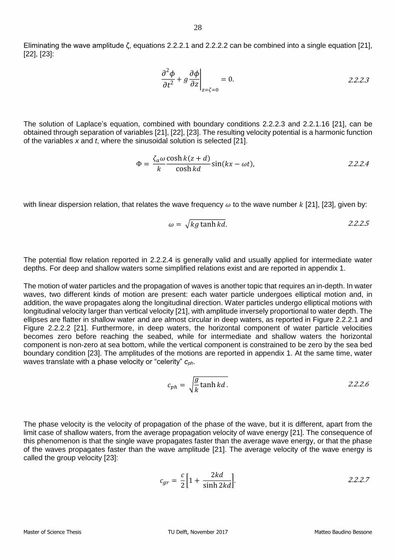
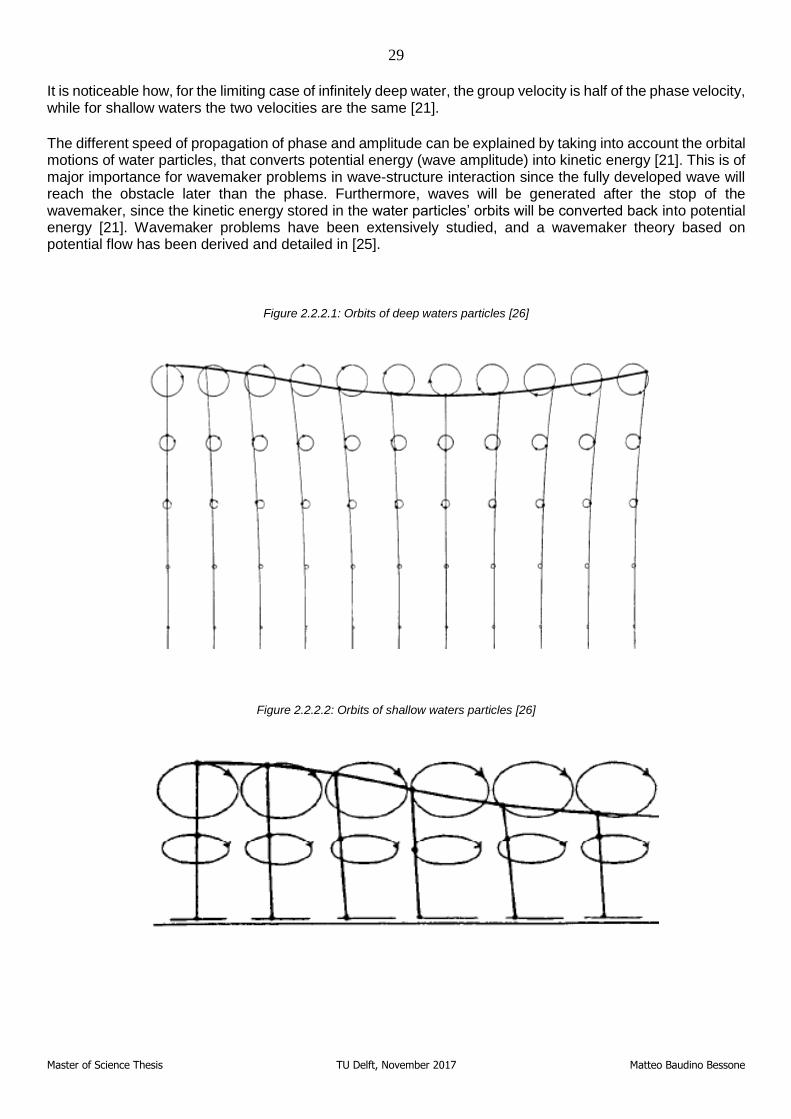
The motion of water particles and the propagation of waves is another topic that requires an in-depth. In water waves, two different kinds of motion are present: each water particle undergoes elliptical motion and, in addition, the wave propagates along the longitudinal direction. Water particles undergo elliptical motions with longitudinal velocity larger than vertical velocity [21], with amplitude inversely proportional to water depth. The ellipses are flatter in shallow water and are almost circular in deep waters, as reported in Figure 2.2.2.1 and Figure 2.2.2.2 [21]. Furthermore, in deep waters, the horizontal component of water particle velocities becomes zero before reaching the seabed, while for intermediate and shallow waters the horizontal component is non-zero at sea bottom, while the vertical component is constrained to be zero by the sea bed boundary condition [23]. The amplitudes of the motions are reported in appendix 1. At the same time, water waves translate with a phase velocity or “celerity” cph.

𝑐𝑝ℎ = √

𝑔

𝑘tanh𝑘𝑑 . 2.2.2.6

The phase velocity is the velocity of propagation of the phase of the wave, but it is different, apart from the limit case of shallow waters, from the average propagation velocity of wave energy [21]. The consequence of this phenomenon is that the single wave propagates faster than the average wave energy, or that the phase of the waves propagates faster than the wave amplitude [21]. The average velocity of the wave energy is called the group velocity [23]:

𝑐𝑔𝑟 =

𝑐

2[1 +

2𝑘𝑑

sinh2𝑘𝑑]. 2.2.2.7

29


It is noticeable how, for the limiting case of infinitely deep water, the group velocity is half of the phase velocity, while for shallow waters the two velocities are the same [21].

The different speed of propagation of phase and amplitude can be explained by taking into account the orbital motions of water particles, that converts potential energy (wave amplitude) into kinetic energy [21]. This is of major importance for wavemaker problems in wave-structure interaction since the fully developed wave will reach the obstacle later than the phase. Furthermore, waves will be generated after the stop of the wavemaker, since the kinetic energy stored in the water particles’ orbits will be converted back into potential energy [21]. Wavemaker problems have been extensively studied, and a wavemaker theory based on potential flow has been derived and detailed in [25].

Figure 2.2.2.1: Orbits of deep waters particles [26]

Figure 2.2.2.2: Orbits of shallow waters particles [26]

30


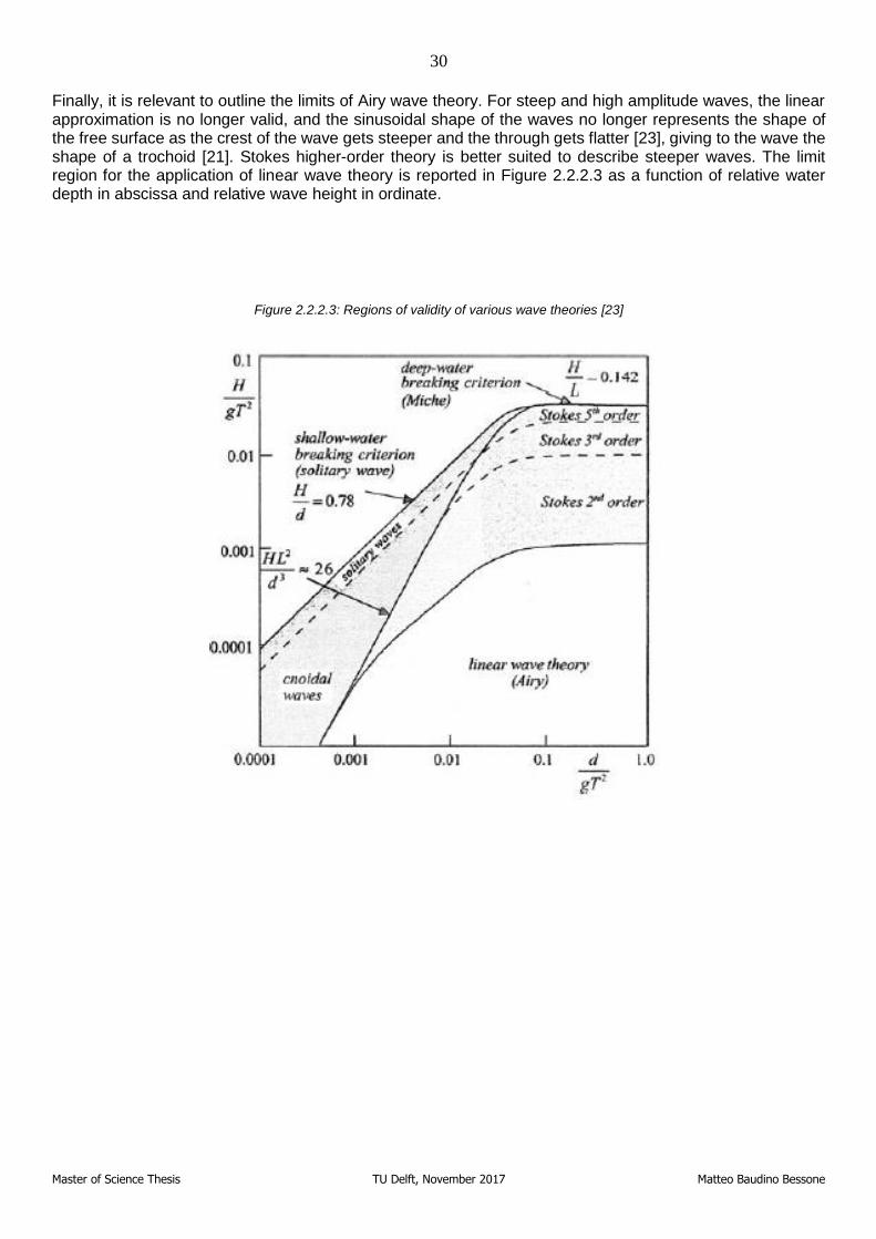
Finally, it is relevant to outline the limits of Airy wave theory. For steep and high amplitude waves, the linear approximation is no longer valid, and the sinusoidal shape of the waves no longer represents the shape of the free surface as the crest of the wave gets steeper and the through gets flatter [23], giving to the wave the shape of a trochoid [21]. Stokes higher-order theory is better suited to describe steeper waves. The limit region for the application of linear wave theory is reported in Figure 2.2.2.3 as a function of relative water depth in abscissa and relative wave height in ordinate.

Figure 2.2.2.3: Regions of validity of various wave theories [23]

31


2.3. Hydromechanics of floating rigid bodies

In this chapter, some significant concepts of hydrodynamics for offshore structures are introduced, focusing on the wave-structure interaction. The objective of hydrodynamic analysis is to solve the pressure distribution around the wetted surface of a structure and the correlated wave and current forces [21]. For a floating body, the forces can be subdivided into hydrostatic forces, hydromechanical forces, depending on the motions of the body in an undisturbed fluid, and wave exciting forces, generated by the incoming waves [26]. In the first subchapter, the hydrostatic and stability of a floating body is briefly treated. In the second section, the hydrodynamic forces are described. Finally, in the third subchapter, the wave-body interaction problem is solved, first for only heave motion and then for the full two-dimensional problem.

2.3.1. Hydrostatic analysis

As it may be noticed from equation 2.2.1.10 and from equation 2.2.1.11, the pressure field exerted from an incoming wave on a body can be separated into a hydrostatic component and a hydrodynamic component. This section focuses on the hydrostatic component.

As Archimedes law states, a point on a body immersed in a fluid undergoes a pressure force from the column of fluid laying above that point [26]. The infinitesimal component of this force, acting on the surface dS can be computed as follows [21]:

𝑑𝐹 = −𝑝ℎ𝒏𝑑𝑆, 2.3.1.1

where 𝒏 is the unit normal vector perpendicular to the surface 𝑑𝑆, that points outwards. The pressure can then be integrated along the wetted surface of the body leading to the resultant hydrostatic force. In the case of a floating or submerged body, only the vertical component remains, that is called buoyancy [26], and is proportional to the displaced volume of fluid Vsub:

𝐹𝑠𝑡 = (0,0, 𝜌𝑔𝑉𝑠𝑢𝑏). 2.3.1.2

For structures that are only partially submerged, or that are subjected to a varying pressure distribution along their surface, as it is the case for pipelines during installation, other components have to be taken into account, apart from the vertical one. The atmospheric pressure can be negligible for floating structures, since it acts on the whole wetted perimeter, but it has to be taken into account for bottom-mounted ones, since the component acting on the underside of the structure perishes [21].

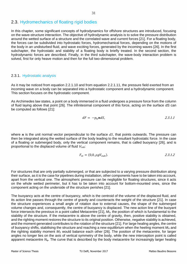
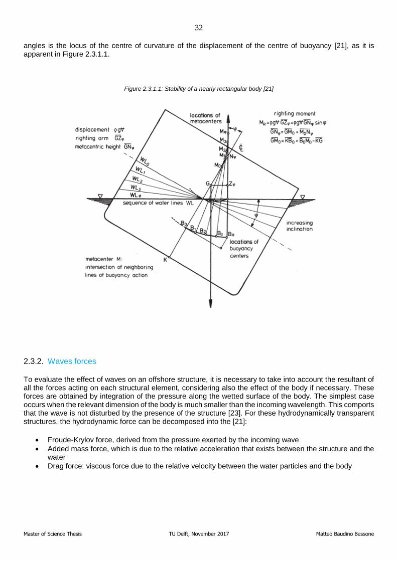
The buoyancy acts at the centre of buoyancy, which is the centroid of the volume of the displaced fluid, and its action line passes through the centre of gravity and counteracts the weight of the structure [21]. In case the structure experiences a small angle of rotation due to external causes, the shape of the submerged volume changes and, consequently, the centre of buoyancy is displaced. The new action line of the buoyant force intersects the previous in a point called Metacentre [21], M0, the position of which is fundamental to the stability of the structure. If the metacentre is above the centre of gravity, then, positive stability is obtained, and the righting moment restores the structure to its original position. Otherwise, negative stability is achieved, and the moment generated contributes to the rotation of the structure [21]. For large healing angles, the centre of buoyancy shifts, stabilising the structure and reaching a new equilibrium when the heeling moment MH and the righting stability moment MS would balance each other [26]. The position of the metacentre, for larger angles no longer lies on the axis of vertical symmetry of the body, while the new interception point is called apparent metacentre Nφ. The curve that is described by the body metacentre for increasingly larger healing

32


angles is the locus of the centre of curvature of the displacement of the centre of buoyancy [21], as it is apparent in Figure 2.3.1.1.

Figure 2.3.1.1: Stability of a nearly rectangular body [21]

2.3.2. Waves forces

To evaluate the effect of waves on an offshore structure, it is necessary to take into account the resultant of all the forces acting on each structural element, considering also the effect of the body if necessary. These forces are obtained by integration of the pressure along the wetted surface of the body. The simplest case occurs when the relevant dimension of the body is much smaller than the incoming wavelength. This comports that the wave is not disturbed by the presence of the structure [23]. For these hydrodynamically transparent structures, the hydrodynamic force can be decomposed into the [21]:

• Froude-Krylov force, derived from the pressure exerted by the incoming wave

• Added mass force, which is due to the relative acceleration that exists between the structure and the water

• Drag force: viscous force due to the relative velocity between the water particles and the body

33


The Froude-Krylov force is derived from the pressure gradient generated by an accelerated fluid interacting with a fixed structure [27]:

𝑑𝐹𝐹𝐾,𝑥 =

𝜕𝑝

𝜕𝑥= −𝜌

𝑑𝑢

𝑑𝑡. 2.3.2.1

The total force acting on the body can be computed by integration around the wetted perimeter, which can be converted in a volume integral applying Gauss theorem. Only the dynamic component due to the incoming wave has to be taken into account [21].

𝐹𝐹𝐾,𝑥 = −∫𝑝 𝒏 𝑑𝑆 = −∫

𝜕𝑝

𝜕𝑥 𝑑𝑉 = ∫𝜌

𝑑𝑢

𝑑𝑡 𝑑𝑉. 2.3.2.2

The added mass force is derived from the mass of the fluid flowing around the body, which is accelerated by the pressure generated by the movements of the body itself [27]. The total force required to accelerate the mass of the fluid m’ and the mass of the body m can be written as [21]:

𝐹𝑎𝑀,𝑥 = 𝐶𝑎𝜌𝑉 (

𝜕𝑢

𝜕𝑡− �̇�𝑏), 2.3.2.3

where 𝐶𝑎 is the added mass coefficient and �̇�𝑏 is the acceleration of the body.

The viscous drag force, associated with wake-related downstream effects, can be written as [21]:

𝐹𝑑,𝑥 = 𝐶𝑑𝜌

2𝐴|𝑢|𝑢, 2.3.2.4

with A being the cross-section of the body and Cd drag coefficient.

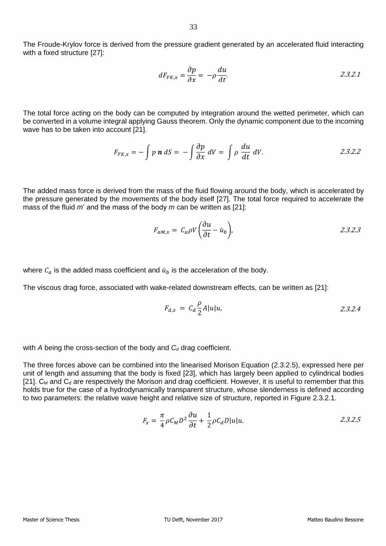
The three forces above can be combined into the linearised Morison Equation (2.3.2.5), expressed here per unit of length and assuming that the body is fixed [23], which has largely been applied to cylindrical bodies [21]. CM and Cd are respectively the Morison and drag coefficient. However, it is useful to remember that this holds true for the case of a hydrodynamically transparent structure, whose slenderness is defined according to two parameters: the relative wave height and relative size of structure, reported in Figure 2.3.2.1.

𝐹𝑥 =

𝜋

4𝜌𝐶𝑀𝐷

2𝜕𝑢

𝜕𝑡+ 1

2𝜌𝐶𝑑𝐷|𝑢|𝑢. 2.3.2.5

34


Figure 2.3.2.1: Loading regimes for vertical circular cylinders [21]

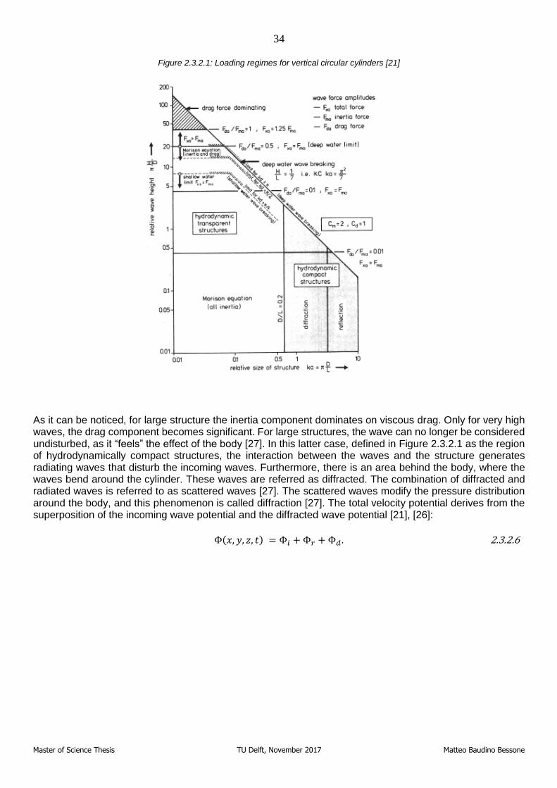
As it can be noticed, for large structure the inertia component dominates on viscous drag. Only for very high waves, the drag component becomes significant. For large structures, the wave can no longer be considered undisturbed, as it “feels” the effect of the body [27]. In this latter case, defined in Figure 2.3.2.1 as the region of hydrodynamically compact structures, the interaction between the waves and the structure generates radiating waves that disturb the incoming waves. Furthermore, there is an area behind the body, where the waves bend around the cylinder. These waves are referred as diffracted. The combination of diffracted and radiated waves is referred to as scattered waves [27]. The scattered waves modify the pressure distribution around the body, and this phenomenon is called diffraction [27]. The total velocity potential derives from the superposition of the incoming wave potential and the diffracted wave potential [21], [26]:

Φ(𝑥, 𝑦, 𝑧, 𝑡) = Φ𝑖 +Φ𝑟 +Φ𝑑 . 2.3.2.6

35


Figure 2.3.2.2: Scattered waves generated by the interaction of a train of regular waves with a large structure [27]

2.3.3. Motions of a floating rigid body under the action of a regular wave train

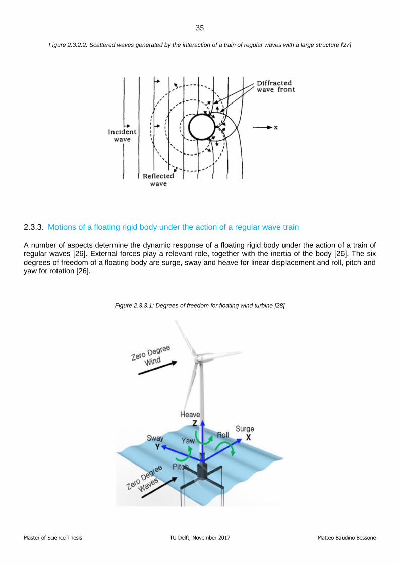
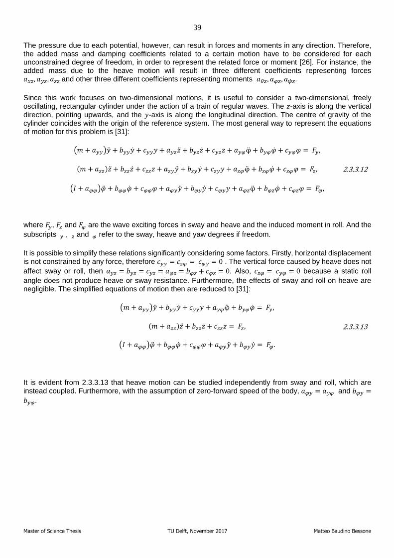
A number of aspects determine the dynamic response of a floating rigid body under the action of a train of regular waves [26]. External forces play a relevant role, together with the inertia of the body [26]. The six degrees of freedom of a floating body are surge, sway and heave for linear displacement and roll, pitch and yaw for rotation [26].

Figure 2.3.3.1: Degrees of freedom for floating wind turbine [28]

36


The problem is firstly approached considering a two-dimensional cylinder moving in heave in deep waters and, afterwards, it is extended to include the remaining degrees of freedom.

In order to solve the motions and forces acting on a floating rigid body, it is useful to subdivide the problem into three different subcases: a floating body in still water, a forced motion case and a fixed case with incoming waves. From the linear superposition of these cases, it is possible to derive the full motions of a floating body subjected to a train of regular waves. Newton’s second law for the heaving cylinder can be written as [26]:

𝑚�̈� = 𝐹ℎ + 𝐹𝑤 , 2.3.3.1

where Fh is the hydromechanical wave forces and Fw the exciting wave force.

For the first case, the only forces to take into account are the gravity force of the body and the buoyancy. Since the body is in equilibrium, these forces cancel out.

For hydromechanically forced motions, Newton’s second law for a heaving cylinder results in [26]:

𝑚�̈� = −𝑚𝑔 + 𝜌(𝑇 − 𝑧)𝐴𝑤 − 𝑏𝑧𝑧�̇� + 𝑎𝑧𝑧𝑧,̈ 2.3.3.2

in which 𝐴𝑤 is the waterplane area. Considering that the weight of the cylinder equals the weight of the

displaced water 𝑚𝑔 = 𝜌𝑇𝐴𝑤, the equation results in [26]:

(𝑚 + 𝑎𝑧𝑧)�̈� + 𝑏𝑧𝑧�̇� + 𝑐𝑧𝑧𝑧 = 0, 2.3.3.3

where the added mass term 𝑎𝑧𝑧�̈� and the damping term 𝑏𝑧𝑧�̇� represent the forces generated by the motions

of the cylinder in the water [26]. The correct evaluation of the added mass and damping coefficient, 𝑎𝑧𝑧 and 𝑏𝑧𝑧 respectively, is crucial for the correct prediction of forces and motions for a floating body subjected to regular waves [29].

The incoming wave force for the case of a fixed, two-dimensional cylinder is the Froude-Krilov force, that has been introduced in the previous chapter. For the limiting case of deep waters, and assuming that the wavelength is large with respect to the diameter of the cylinder 2𝐷, it can be represented as [26]:

𝐹𝐹𝐾 = 𝑐𝑧𝑧𝜁∗ = 𝜌𝑔2𝐷𝑒−𝑘𝑇𝜁 cos𝜔𝑡, 2.3.3.4

in which ζ* is the reduced wave height equal to:

𝜁∗ = 𝜁𝑒−𝑘𝑇 cos𝜔𝑡. 2.3.3.5

37


Diffraction has also to be taken into account. The diffraction of waves by large structures has been a comprehensively studied, and a formulation for the diffracted velocity potential has been given by MacCamy and Fuchs [30].

The effects of diffraction can be considered by assuming the existence of additional force components that are proportional to the velocity and the acceleration of the water particles. The wave force can then be expressed as [26]:

𝐹𝑤 = 𝑎𝑧𝑧𝜁̈∗ + 𝑏𝑧𝑧𝜁̇

∗ + 𝑐𝑧𝑧𝜁∗. 2.3.3.6

It is now possible to write the equation of motion for a heaving cylinder as [26]:

(𝑚 + 𝑎𝑧𝑧)�̈� + 𝑏𝑧𝑧�̇� + 𝑐𝑧𝑧𝑧 = 𝑎𝑧𝑧𝜁̈∗ + 𝑏𝑧𝑧𝜁̇

∗ + 𝑐𝑧𝑧𝜁∗. 2.3.3.7

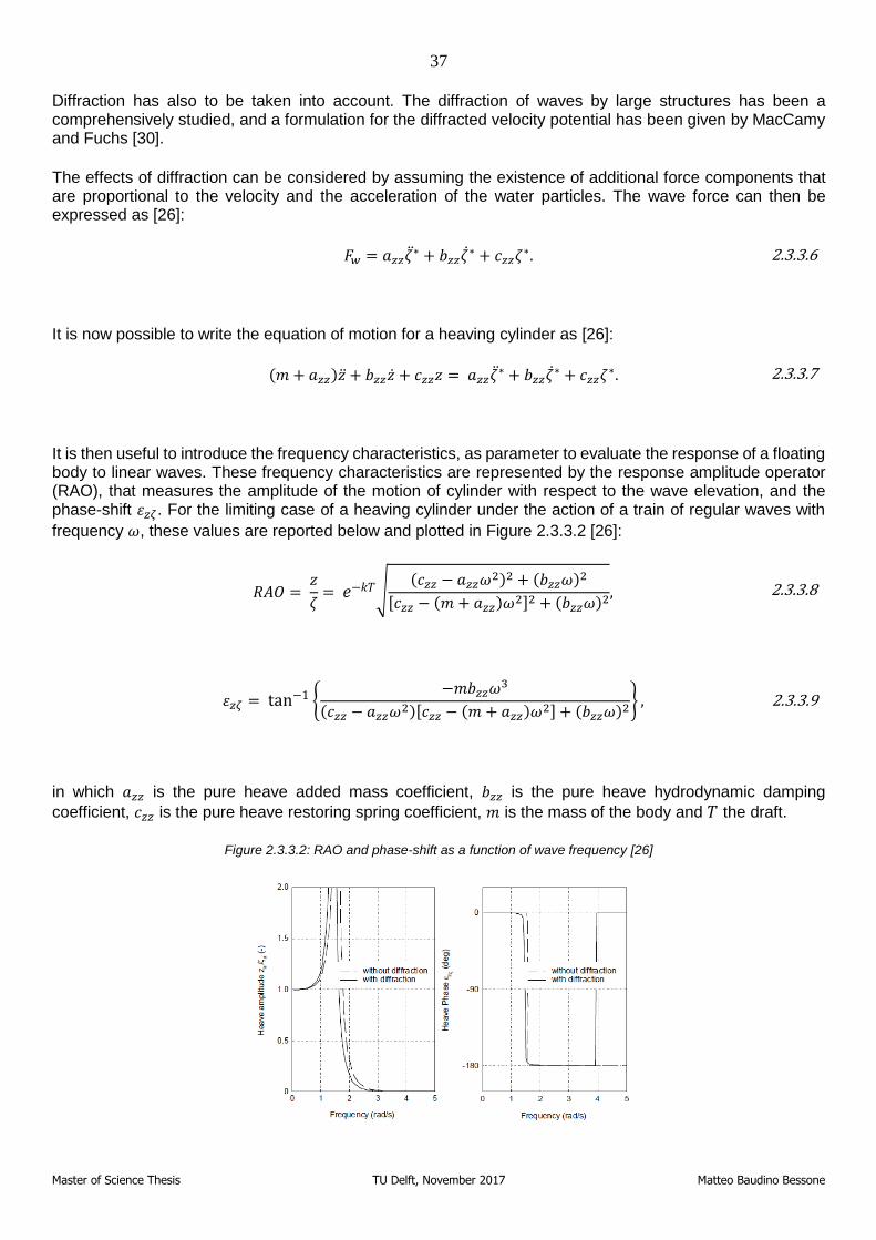
It is then useful to introduce the frequency characteristics, as parameter to evaluate the response of a floating body to linear waves. These frequency characteristics are represented by the response amplitude operator (RAO), that measures the amplitude of the motion of cylinder with respect to the wave elevation, and the phase-shift 𝜀𝑧𝜁. For the limiting case of a heaving cylinder under the action of a train of regular waves with

frequency 𝜔, these values are reported below and plotted in Figure 2.3.3.2 [26]:

𝑅𝐴𝑂 = 𝑧

𝜁= 𝑒−𝑘𝑇√

(𝑐𝑧𝑧 − 𝑎𝑧𝑧𝜔2)2 + (𝑏𝑧𝑧𝜔)

2

[𝑐𝑧𝑧 − (𝑚 + 𝑎𝑧𝑧)𝜔2]2 + (𝑏𝑧𝑧𝜔)

2, 2.3.3.8

𝜀𝑧𝜁 = tan

−1 {−𝑚𝑏𝑧𝑧𝜔

3

(𝑐𝑧𝑧 − 𝑎𝑧𝑧𝜔2)[𝑐𝑧𝑧 − (𝑚 + 𝑎𝑧𝑧)𝜔

2] + (𝑏𝑧𝑧𝜔)2} , 2.3.3.9

in which 𝑎𝑧𝑧 is the pure heave added mass coefficient, 𝑏𝑧𝑧 is the pure heave hydrodynamic damping

coefficient, 𝑐𝑧𝑧 is the pure heave restoring spring coefficient, 𝑚 is the mass of the body and 𝑇 the draft.

Figure 2.3.3.2: RAO and phase-shift as a function of wave frequency [26]

38


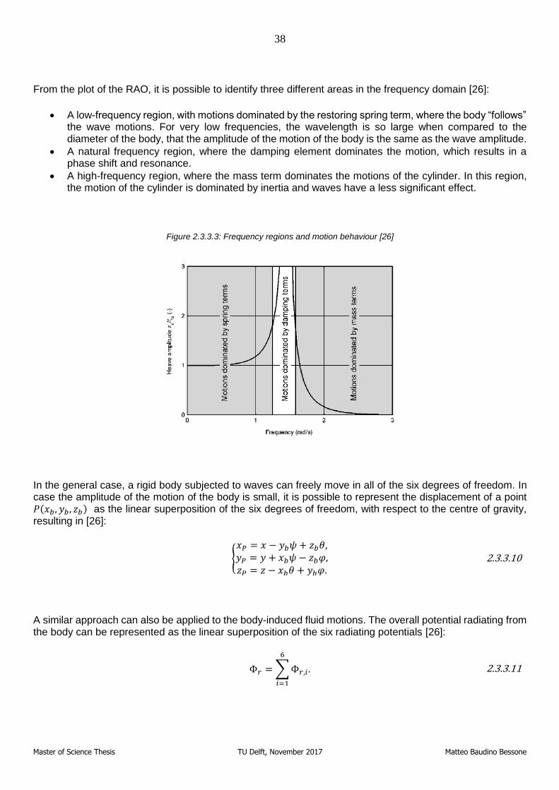
From the plot of the RAO, it is possible to identify three different areas in the frequency domain [26]:

• A low-frequency region, with motions dominated by the restoring spring term, where the body “follows” the wave motions. For very low frequencies, the wavelength is so large when compared to the diameter of the body, that the amplitude of the motion of the body is the same as the wave amplitude.

• A natural frequency region, where the damping element dominates the motion, which results in a phase shift and resonance.

• A high-frequency region, where the mass term dominates the motions of the cylinder. In this region, the motion of the cylinder is dominated by inertia and waves have a less significant effect.

Figure 2.3.3.3: Frequency regions and motion behaviour [26]

In the general case, a rigid body subjected to waves can freely move in all of the six degrees of freedom. In case the amplitude of the motion of the body is small, it is possible to represent the displacement of a point 𝑃(𝑥𝑏 , 𝑦𝑏 , 𝑧𝑏) as the linear superposition of the six degrees of freedom, with respect to the centre of gravity, resulting in [26]:

{

𝑥𝑃 = 𝑥 − 𝑦𝑏𝜓 + 𝑧𝑏𝜃,𝑦𝑃 = 𝑦 + 𝑥𝑏𝜓 − 𝑧𝑏𝜑,𝑧𝑃 = 𝑧 − 𝑥𝑏𝜃 + 𝑦𝑏𝜑.

2.3.3.10

A similar approach can also be applied to the body-induced fluid motions. The overall potential radiating from the body can be represented as the linear superposition of the six radiating potentials [26]:

Φ𝑟 =∑Φ𝑟,𝑖

6

𝑖=1

. 2.3.3.11

39


The pressure due to each potential, however, can result in forces and moments in any direction. Therefore, the added mass and damping coefficients related to a certain motion have to be considered for each unconstrained degree of freedom, in order to represent the related force or moment [26]. For instance, the added mass due to the heave motion will result in three different coefficients representing forces 𝑎𝑥𝑧, 𝑎𝑦𝑧, 𝑎𝑧𝑧 and other three different coefficients representing moments 𝑎𝜃𝑧, 𝑎𝜑𝑧, 𝑎𝜓𝑧.

Since this work focuses on two-dimensional motions, it is useful to consider a two-dimensional, freely oscillating, rectangular cylinder under the action of a train of regular waves. The 𝑧-axis is along the vertical direction, pointing upwards, and the 𝑦-axis is along the longitudinal direction. The centre of gravity of the cylinder coincides with the origin of the reference system. The most general way to represent the equations of motion for this problem is [31]:

(𝑚 + 𝑎𝑦𝑦)�̈� + 𝑏𝑦𝑦�̇� + 𝑐𝑦𝑦𝑦 + 𝑎𝑦𝑧�̈� + 𝑏𝑦𝑧�̇� + 𝑐𝑦𝑧𝑧 + 𝑎𝑦𝜑φ̈ + 𝑏𝑦𝜑�̇� + 𝑐𝑦𝜑𝜑 = 𝐹𝑦,

(𝑚 + 𝑎𝑧𝑧)�̈� + 𝑏𝑧𝑧�̇� + 𝑐𝑧𝑧𝑧 + 𝑎𝑧𝑦�̈� + 𝑏𝑧𝑦�̇� + 𝑐𝑧𝑦𝑦 + 𝑎𝑧𝜑φ̈ + 𝑏𝑧𝜑�̇� + 𝑐𝑧𝜑𝜑 = 𝐹𝑧,

(𝐼 + 𝑎𝜑𝜑)�̈� + 𝑏𝜑𝜑�̇� + 𝑐𝜑𝜑𝜑 + 𝑎𝜑𝑦�̈� + 𝑏𝜑𝑦�̇� + 𝑐𝜑𝑦𝑦 + 𝑎𝜑𝑧φ̈ + 𝑏𝜑𝑧�̇� + 𝑐𝜑𝑧𝜑 = 𝐹𝜑,

2.3.3.12

where 𝐹𝑦, 𝐹𝑧 and 𝐹𝜑 are the wave exciting forces in sway and heave and the induced moment in roll. And the

subscripts 𝑦 , 𝑧 and 𝜑 refer to the sway, heave and yaw degrees if freedom.

It is possible to simplify these relations significantly considering some factors. Firstly, horizontal displacement is not constrained by any force, therefore 𝑐𝑦𝑦 = 𝑐𝑧𝜑 = 𝑐𝜑𝑦 = 0 . The vertical force caused by heave does not

affect sway or roll, then 𝑎𝑦𝑧 = 𝑏𝑦𝑧 = 𝑐𝑦𝑧 = 𝑎𝜑𝑧 = 𝑏𝜑𝑧 + 𝑐𝜑𝑧 = 0. Also, 𝑐𝑧𝜑 = 𝑐𝑦𝜑 = 0 because a static roll

angle does not produce heave or sway resistance. Furthermore, the effects of sway and roll on heave are negligible. The simplified equations of motion then are reduced to [31]:

(𝑚 + 𝑎𝑦𝑦)�̈� + 𝑏𝑦𝑦�̇� + 𝑐𝑦𝑦𝑦 + 𝑎𝑦𝜑φ̈ + 𝑏𝑦𝜑�̇� = 𝐹𝑦,

(𝑚 + 𝑎𝑧𝑧)�̈� + 𝑏𝑧𝑧�̇� + 𝑐𝑧𝑧𝑧 = 𝐹𝑧,

(𝐼 + 𝑎𝜑𝜑)�̈� + 𝑏𝜑𝜑�̇� + 𝑐𝜑𝜑𝜑 + 𝑎𝜑𝑦�̈� + 𝑏𝜑𝑦�̇� = 𝐹𝜑.

2.3.3.13

It is evident from 2.3.3.13 that heave motion can be studied independently from sway and roll, which are instead coupled. Furthermore, with the assumption of zero-forward speed of the body, 𝑎𝜑𝑦 = 𝑎𝑦𝜑 and 𝑏𝜑𝑦 =

𝑏𝑦𝜑.

40


3. Numerical Background

In this section, the most relevant aspects related to the numerical experiments that are discussed in this thesis are reported. The first chapter introduces the governing equations and the discretisation methods. The second and third sections deal with the two discretisation pairs and the numerical set-ups that have been applied for the simulations. In the last chapter, the immersed-body method for wave-structure interaction is presented.

The software that has been used to solve the Navier-Stokes equations numerically for this work is fluidity. Fluidity can solve multi-material and multiphase problems on structured and unstructured finite element meshes. Furthermore, it includes a useful Python interface to prescribe fields and access the state of the whole system [32].

3.1. Governing Equations and discretisation

In this subchapter, the Navier-Stokes equations are presented, first in the most general formulation and then for purely hydrodynamic problems. In the following sections, the discretisation methods available in fluidity are introduced and briefly described.

3.1.1. The Navier-Stokes equations

The flow of a continuous fluid is usually described by the Navier-Stokes equations, which define the conservation of mass, momentum and energy [33]. In their most conservative form, they can be written as [33], [34]:

𝜕𝜌

𝜕𝑡+ ∇ ∙ (𝜌𝒗) = 0, 3.1.1.1

𝜕(𝜌𝒗)

𝜕𝑡+ ∇ ∙ (𝜌𝒗𝒗 − �̿�) = 𝑭, 3.1.1.2

𝜕(𝜌𝑬)

𝜕𝑡+ ∇ ∙ (𝜌𝑬𝒗 − �̿�𝒗 + 𝒒) = 𝑭 ∙ 𝒗, 3.1.1.3

where 𝒗 is the velocity vector, ρ is the density of the fluid, �̿� is the stress tensor, 𝑭 represents a source term, for example the body force, 𝑬 is the total specific energy and 𝒒 the thermic flux.

41


For incompressible fluids, and considering only the continuity and momentum equations (3.1.1.1 and 3.1.1.2), for a purely hydrodynamic problem, it is possible to simplify the Navier-Stokes equations as follows [6]:

𝛻 ∙ 𝒗 = 0, 3.1.1.4

𝜌𝜕𝒗

𝜕𝑡+ 𝜌(𝒗 ∙ ∇)𝒗 = −∇𝑝 + ∇ ∙ (2𝜇𝑆̿) + 𝑭, 3.1.1.5

where the stress tensor �̿� has been subdivided into a mean part (pressure), −∇𝑝, and a deviatoric part, 𝑆̿.

3.1.2. The discretisation method

It is not possible to solve the Navier-Stokes equations analytically, apart from some simplified cases. Therefore, a numerical method has to be applied to solve the problem. To find the numerical solution, it is necessary to subdivide the time domain and the space domain into a finite set of components [35]. Different schemes exist to discretise partial differential equations, that can be roughly subdivided into [33]:

• Finite difference methods, where the derivatives of the differential equation are approximated by a combination of the values of the function at the grid points.

• Finite volume methods that take into account the integral mass, momentum and energy balances about each element to find the discretised values.

• Finite element methods that subdivide the domain into different elements and represent on each element the dependent variables by means of a shape function.

The formulation of the FE methods usually starts with the introduction of the weak form of the differential equations [33] to be discretised. This form is usually introduced following four steps [35]:

• Multiply the equation with an arbitrary function, called a test function

• Perform the integration of the equation over the domain of the problem

• Integrate by part to lower the order of the derivative and the smoothness required for the solution

• Introduce the natural boundary conditions while integrating by parts

The following step to perform is to substitute the continuous space of the test functions and of the solution functions, also called trial space, with a reduced, discrete space. This substitution implies that the test and trial solution spaces become discrete and, therefore, can be represented using the discrete points of a mesh of elements [33]. It is then possible to represent an arbitrary function with a certain number of prescribed functions and discretionary parameters [35]:

�̂�(𝒙𝒊, 𝒕) = ∑𝝓𝒏(𝒙𝒊)𝒖𝒏(𝒕) + 𝒖𝒃(𝒙𝒊, 𝒕),

𝑵

𝒏=𝟏

3.1.2.1

�̂�(𝑥𝑖, 𝑡) = ∑ 𝜓𝑚(𝑥𝑖)𝑤𝑚(𝑡)

𝑁

𝑚=1

, 3.1.2.2

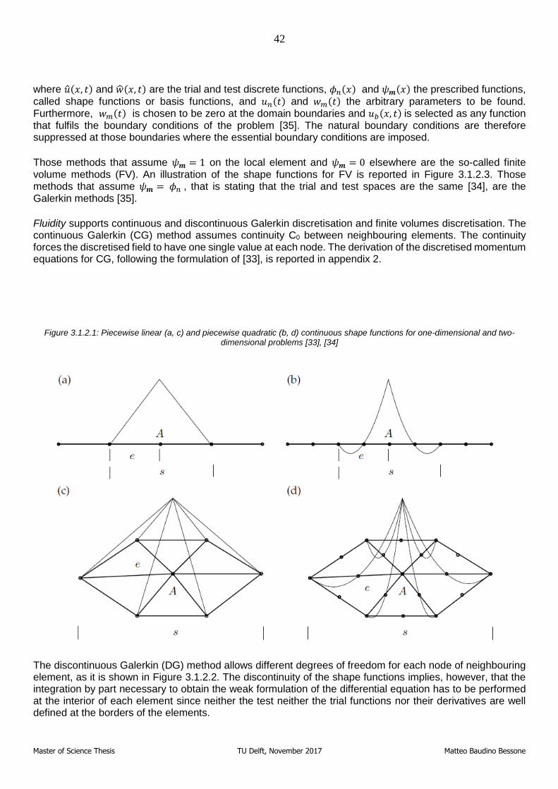
42


where �̂�(𝑥, 𝑡) and �̂�(𝑥, 𝑡) are the trial and test discrete functions, 𝜙𝑛(𝑥) and 𝜓𝒎(𝑥) the prescribed functions,

called shape functions or basis functions, and 𝑢𝑛(𝑡) and 𝑤𝑚(𝑡) the arbitrary parameters to be found. Furthermore, 𝑤𝑚(𝑡) is chosen to be zero at the domain boundaries and 𝑢𝑏(𝑥, 𝑡) is selected as any function that fulfils the boundary conditions of the problem [35]. The natural boundary conditions are therefore suppressed at those boundaries where the essential boundary conditions are imposed.

Those methods that assume 𝜓𝒎 = 1 on the local element and 𝜓𝒎 = 0 elsewhere are the so-called finite volume methods (FV). An illustration of the shape functions for FV is reported in Figure 3.1.2.3. Those methods that assume 𝜓𝒎 = 𝜙𝑛 , that is stating that the trial and test spaces are the same [34], are the Galerkin methods [35].

Fluidity supports continuous and discontinuous Galerkin discretisation and finite volumes discretisation. The continuous Galerkin (CG) method assumes continuity C0 between neighbouring elements. The continuity forces the discretised field to have one single value at each node. The derivation of the discretised momentum equations for CG, following the formulation of [33], is reported in appendix 2.

Figure 3.1.2.1: Piecewise linear (a, c) and piecewise quadratic (b, d) continuous shape functions for one-dimensional and two-dimensional problems [33], [34]

The discontinuous Galerkin (DG) method allows different degrees of freedom for each node of neighbouring element, as it is shown in Figure 3.1.2.2. The discontinuity of the shape functions implies, however, that the integration by part necessary to obtain the weak formulation of the differential equation has to be performed at the interior of each element since neither the test neither the trial functions nor their derivatives are well defined at the borders of the elements.

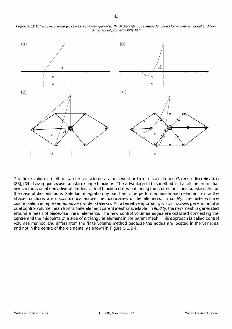
43


Figure 3.1.2.2: Piecewise linear (a, c) and piecewise quadratic (b, d) discontinuous shape functions for one-dimensional and two-dimensional problems [33], [34]

The finite volumes method can be considered as the lowest order of discontinuous Galerkin discretisation [33], [34], having piecewise constant shape functions. The advantage of this method is that all the terms that involve the spatial derivative of the test or trial function drops out, being the shape functions constant. As for the case of discontinuous Galerkin, integration by part has to be performed inside each element, since the shape functions are discontinuous across the boundaries of the elements. In fluidity, the finite volume discretisation is represented as zero-order Galerkin. An alternative approach, which involves generation of a dual control volume mesh from a finite element parent mesh is available. In fluidity, the new mesh is generated around a mesh of piecewise linear elements. The new control volumes edges are obtained connecting the centre and the midpoints of a side of a triangular element in the parent mesh. This approach is called control volumes method and differs from the finite volume method because the nodes are located in the vertexes and not in the centre of the elements, as shown in Figure 3.1.2.4.

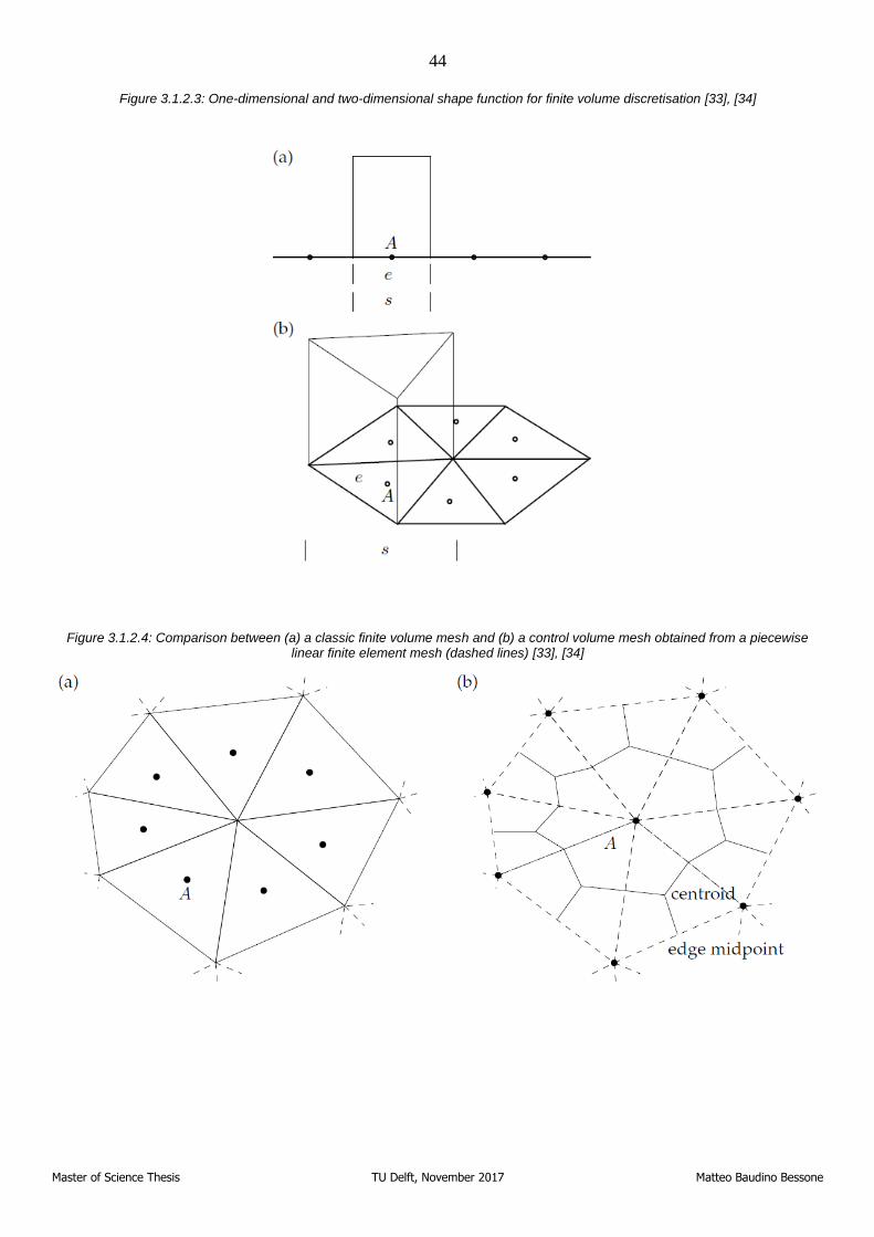
44


Figure 3.1.2.3: One-dimensional and two-dimensional shape function for finite volume discretisation [33], [34]

Figure 3.1.2.4: Comparison between (a) a classic finite volume mesh and (b) a control volume mesh obtained from a piecewise linear finite element mesh (dashed lines) [33], [34]

45


3.2. The fluidity P1DG-P2 set-up

Different criteria can be considered when choosing a suitable velocity-pressure basis functions pair for a certain problem has to be chosen. One consideration that can be made is to identify which is the most relevant term in the Navier-Stokes equations for the selected case. Oceanic flows are usually inertia dominated. Therefore, the suggested velocity-pressure basis function pair for oceanic flows in fluidity is the P1DG-P2, which indicates linear discontinuous Galerkin elements for velocity and quadratic continuous Galerkin elements for pressure [34]. The advantages of this method are the absence of spurious modes, namely high-frequency disturbances that contaminate the desired wave spectrum, and that the geostrophic balance is well represented [36]. For the purpose of this work, the absence of spurious modes is of primary importance and therefore this is the selected pair for ocean waves simulations.

Since the problem is purely hydrodynamic, the equations discretised with this method are the continuity and momentum equations, with the Boussinesq approximation [6] 3.1.1.4, 3.1.1.5.

The domain represented is a numerical wave basin, where waves are generated at the inlet and damped out at the end. To adequately define the problem, one boundary condition has to be applied at each side of the domain. The inlet velocity boundary condition is applied weakly and prescribes the horizontal velocity simulating thereby a piston-type wavemaker. The input parameters for modelling the wavelength and steepness of the wave generated are the product wave number k per wave amplitude ζ, the water depth d and the wave period T. The exact wave number is computed via dispersion relation. The wavemaker, whose detailed features are reported in the literature [37], is capable of generating 5th order Stokes waves. A smooth start is applied to the wave maker, to simulate real wave basin, with the steady-state velocity being reached after 3 seconds.

A slip wall boundary condition is applied at the sea-bed which prescribes no normal flow, to simulate the oceanic seabed. Homogeneous Neumann boundary conditions are enforced at the end of the domain, letting the water flow in and out of the domain. A kinematic boundary condition is applied at the free surface, ensuring that [37]:

𝜕𝜁

𝜕𝑡= 𝒗 ∙ 𝒏

𝒏 ∙ �̂�, 3.2.1

in which n is a unit vector normal to the free surface.

At the far end of the domain an absorption layer is implemented, to avoid reflections of the wave back into the physical domain. The sponge-layer is obtained introducing an additional absorption term to the right side of the Navier-Stokes equation, which is proportional to the velocity 𝒗 and a constant σ [6]:

𝜎 =

{

1

4{tanh [

sin(𝜋(4𝑥 − 1)/2)

1 − (4𝑥 − 1)2] + 1} 𝑖𝑓 0 ≤ 𝑥 ≤

1

2,

1

4{tanh [

sin(𝜋(3 − 4�̌�)/2)

1 − (3 − 4𝑥)2] + 1} 𝑖𝑓 0 ≤ 𝑥 ≤

1

2,

3.2.2

where 𝑥 is the ratio of the difference between the actual coordinate and the beginning of the sponge layer,

𝑥 − 𝐿, and the length of the sponge layer L0. Furthermore, the mesh is coarsened progressively in the absorption layer, to dissipate numerically the waves. The set-up is discretised in time using a Crank-Nicolson scheme.

46


3.3. The fluidity P0-P1CV set-up

To allow the heave and rotation motion of the floating body, a computational domain containing both air and water has to be generated, and an interface between the two fluids has to be created. One of the main issues, for problems that involve multiple immiscible fluids, is to avoid large numerical diffusion at the interface, which generates an unphysical mixture of materials and smearing of the interface. The generation of jetsam and flotsam, bubbles of one material suspended in the other material, is another issue typical of multi-material simulations [33]. The multi-material configuration of fluidity allows the representation of incompressible, immiscible fluids separated maintaining a sharp interface [34]. An in-depth description of the approach is reported in the literature [33], here only the main aspects are highlighted.

There exist different material tracking methods to represent multi-material flows of immiscible fluids. One way is to generate a mesh that reproduces the interfaces. This mesh must be adapted to follow the interface motion. However, for problems that involve significant motion, this method is unsuitable, leading to substantial deformations in the mesh. The advection of tracers that define the location of the separate fluids is instead the solution adopted by Eulerian methods. These approaches can be categorised into non-field based or field based, depending on whether the advected tracer is a field or not [33].

The volume of fluids methods is a subdomain of the field based approaches. In these methods, a volume fraction of each material is used to reconstruct the interface. The gradient of the volume fraction defines the interface orientation, while the actual volume fraction retrieves the interface position [33]. This latter is the method which is applied in fluidity. Through the material volume fraction field, the bulk properties of the fluid can be expressed as [34]:

𝜌 =∑𝜌𝑖𝑐𝑖

𝑁

𝑖=1

, 3.3.1

𝜇 =∑𝜇𝑖

𝑁

𝑖=1

𝑐𝑖 , 3.3.2

where 𝜌 and 𝜇 are the bulk density and viscosity of the fluid, 𝑐𝑖 is the material volume fraction (tracer), and 𝜌𝑖 and 𝜇𝑖 are the density and dynamic viscosity of the ith fluid.

Making use of equations 3.3.1 and 3.3.2, the Navier-Stokes equation for the ith the fluid present in the domain can be expressed as [6]:

𝜕𝑐𝑖𝜌𝑖𝜕𝑡

+ ∇ ∙ (𝑐𝑖𝜌𝑖𝒗𝑖) = 0, 3.3.3

𝜕𝑐𝑖𝜌𝑖𝒗𝑖𝜕𝑡

+ ∇ ∙ (𝑐𝑖𝜌𝑖𝒗𝑖)𝒗𝑖 = −𝑐𝑖∇𝑝+ ∇ ∙ (2𝜇𝑐𝑖𝑆�̿�)+ 𝑐𝑖𝜌𝑖𝑔𝒌, 3.3.4

with 𝒌 unit normal vector along the vertical direction. For the specific case analysed in this work, that is when

only two fluids are taken into account, just one velocity field has to be solved, since the velocity profile is the same for both the fluids.

47


In order to track the advection of the tracer, an additional equation is solved [6]:

𝜕𝑐𝑖𝜕𝑡

+ ∇ ∙ (𝑐𝑖𝒗𝑖) = 0. 3.3.5

A significant criterion to choose the discretisation pair for multi-material simulations is to assure the boundedness of the material volume fraction. A tracer concentration lower than zero or larger than one is non-physical and leads to negative bulk densities or negative viscosities in equations 3.3.1 and 3.3.2. Finite volume discretisation is an optimum way to obtain boundedness, combined with an HyperC limiter for advective fluxes. Therefore, the selected discretisation pair is P0-P1CV which assumes piecewise constant basis functions for velocity and piecewise constant control volume basis functions for pressure, derived from a piecewise linear continuous parent mesh. The use of control volumes allows the advective velocity to be divergence-free in the advection equation for the material volume fraction [6].

The numerical domain that is implemented is similar to the one presented in the previous chapter for P1DG-P2 discretisation, with two main differences. Firstly, the boundary condition applied at the end of the domain is a no-normal flow boundary condition instead of a homogeneous Neumann boundary condition, and a homogeneous Neumann boundary condition is applied at the top of the domain instead of the free-surface boundary condition. Secondly, the mesh is significantly refined around the interface, to limit further the smearing of the interface.

48


3.4. The immersed-body method for fluid-structure interaction

When solving the fluid-structure interaction problem of a body subjected to water waves, various approaches are possible. The defined-body method consists in solving the Navier-Stokes equations excluding the volume of the body from the computational domain. This method is effective for fixed structures, but it comports some disadvantages for moving bodies. If the structure is in motion, the defined-body approach requires re-meshing to adapt to the new position of the body, which is computationally expensive, and it can generate distorted grids [6], [10], [38]. The family of the immersed-body methods, instead, models the presence of the structure applying body forces to the fluid on a mesh covering both the regions of the space occupied by the fluid and the solid [6], [10]. Since the presence of the structure is defined in the fluid mesh by adding an extra forcing term to the momentum equation, these methods can be further broadly categorized into continuous forcing methods and direct forcing methods. Continuous forcing methods include the forcing term before discretisation, while direct forcing methods introduce the forcing term in the already discretised equation. For the purposes of this work, the continuous forcing method is considered, and therefore this section will focus on this approach.

In the selected method, a penalty body force term is introduced into the Navier-Stokes equations, before discretisation, as part of the source terms, in order to relax the body and fluid velocities to each other in the vicinity of the body [6], [10], [38], [39]. The Navier-Stokes equations are solved in the extended domain, that covers both the regions occupied by the fluid and the solid, detected by Vf and Vs respectively [6], [38]. A monolithic velocity is defined on the extended domain, which is a sort of weighted average between of the fluid and solid velocities [6], [10], [38], [39] :

𝝂 = 𝛼𝑓𝝂𝑓 + 𝛼𝑠𝝂𝑠, 3.4.1

where αf and αs are the fluid and the solid concentration fields, respectively. The term 𝛼𝑠 is defined as the ratio of the solid volume to the total volume, while the term 𝛼𝑓 is defined as the ratio of the fluid volume to the

total volume [6], [38], [39], [10].

𝛼𝑓 =

𝑉𝑓

𝑉, 3.4.2

𝛼𝑠 =

𝑉𝑠𝑉. 3.4.3

The penalty term is directly proportional to both the solid concentration field and to the difference between the solid and monolithic velocities [6], [39]:

𝐹 = 𝛽𝛼𝑠(𝒗𝑠 − 𝒗). 3.4.4

This formulation of the penalty term ensures a non-zero force only in the region of the domain where the solid concentration field is non-zero. In expression 3.4.4, a relaxation factor β is introduced, that dictates how fast the solid and fluid velocities relax to each other in the vicinity of the solid body. The formulation of the relaxation factor depends on whether inertia or viscosity dominates the flow [6].

49


𝛽 = 𝑚𝑎𝑥 (𝜌𝑓

Δ𝑡,𝜐

𝐿2), 3.4.5

in which Δ𝑡 is the timestep size, 𝜐 is the kinematic viscosity of the fluid and 𝐿 is the local edge length [10]. For gravity waves-related problems, the inertia is usually the dominating term, therefore the first formulation is adopted.

A supermesh generated from the volume intersection of the fluid mesh and the solid mesh is used to transfer the solid concentration field from the solid mesh to the fluid mesh. The projection is actuated via Galerkin projection [40], thereby preserving the solid volume. Therefore, it can be verified that [6]:

∫ 𝛼𝑠𝑑𝑉 = ∫ 𝑑𝑉

𝑉𝑠

= 𝑉𝑆,

𝑉𝑓

3.4.6

where 𝑉𝑓 is the fluid domain and 𝑉𝑆 is the solid domain.

With the insertion of this penalty term, the Navier-Stokes equations on the extended mesh become [6]:

∇ ∙ 𝒗 = 0, 3.4.7

𝜌𝜕𝒗

𝜕𝑡+ 𝜌(𝒗 ∙ ∇)𝒗 = −∇𝑝 + ∇ ∙ (2𝜇𝑆̿) + 𝐵 + 𝐹. 3.4.8

50


4. The Python code

In this section of the thesis, the main features of the Python-developed code that has been used to compute the rigid-body motions of the floater are introduced. A simple test-case is presented that shows the validity of the code. In the second subchapter, the staggered fluid-structure interaction algorithm is presented. In the last subsection the pressure-integration function, which computes the resultant of the pressure forces on the body, is presented.

4.1. The rigid body code

The dynamics of the rigid body that represents the floater of the floating wind turbine are simulated using a Python code that solves both the balance of linear momentum and the balance of angular momentum for a rigid body. An implicit Newmark scheme is applied to the time integration of the equations of motions, to compute both the linear and angular displacement.

�̅�𝑡+1 = �̅�𝑡 + ((1 − 𝛾)�̅�𝑡 + 𝛾�̅�𝑡+1)Δ𝑡, 4.1.1

�̅�𝑡+1 = �̅�𝑡 + �̅�𝑡Δ𝑡 + ((

1

2− 𝛽) �̅�𝑡 + 𝛽�̅�𝑡+1)Δ𝑡2, 4.1.2

in which �⃗� 𝑡+1 = [𝑥𝑡+1, 𝑦𝑡+1, 𝜃𝑡+1], �̅�𝑡+1 = [�̇�𝑡+1, �̇�𝑡+1, �̇�𝑡+1], and �̅�𝑡+1 = [�̈�𝑡+1, �̈�𝑡+1, �̈�𝑡+1], are the position,

velocity and acceleration vectors, respectively, at timestep t+1, �̅�𝑡, �̅�𝑡 and �̅�𝑡 are the position, velocity and acceleration vectors, respectively, at timestep t and Δ𝑡 is the timestep size. The two parameters 𝛾 and 𝛽 are

chosen, respectively, to be 1

2 and

1

4, so the formulation is trapezoidal.

The code uses NURBS as a model to represent the shape of the body. A complete discussion about NURBS is not relevant to this work, as the implemented geometry is extremely simple. For a complete treatment of NURBS and their properties, there are various pertinent references in the literature [41], [42], [43]. Hereafter, only the most relevant features of NURBS that have been applied in this work will be discussed.

NURBS are the most widespread computation geometry technology [41]. Therefore, they are the most suitable candidate to be applied to the field of isogeometric analysis, as an attempt to merge the areas of CAD and finite element analysis. The idea behind the isogeometric analysis is to obtain a single geometry to utilise both for design and in the FEA, avoiding the loss of accuracy which occurs when converting a CAD model to a FE mesh. The main advantages of NURBS are their precision for representing shapes, the existence of multiple and straightforward methods to refine a NURBS mesh, and the presence of various algorithms to generate NURBS surfaces [41].

In NURBS there exist two different concepts of mesh: the control mesh and the physical mesh. The control mesh does not represent the physical geometry of the NURBS’ object but it controls its conformation. It is made of control elements, which are delimited by control points. The physical mesh, instead, is a representation of the real geometry, and it is composed of two different elements, patches and knot spans. Patches can be conceived as a subdomain of the geometry. The geometry represented in this work is formed

51


by one single patch. Knot spans are the smallest objects that are taken into account when generating a NURBS geometry. They are delimited by knot points [41]. Control points, patches and knot points have all two representations, one in the parametric domain and one in the physical space.

A NURBS object in n dimensions is built from the projection of a n+1-dimensional B-spline object. A NURBS curve 𝐶(𝜉), in n dimensions and defined by (𝑩𝑖)𝑛 control points, is obtained projecting the control points of a B-spline curve of dimension n+1 with control points (𝑩𝑖

𝑠)𝑛 following the relation:

(𝑩𝑖)𝑛 =

(𝑩𝑖𝑠)𝑛𝜛𝑖

, 4.1.3

in which 𝜛𝑖 is the weight of the ith control point.

𝜛𝑖 = (𝐵𝑖𝑠)𝑛+1. 4.1.4

To obtain the desired shape for this work, the weights of the control points 𝜛𝑖 have been chosen to be all identical and equal to one. Under this assumption, it is possible to notice, from equation 4.1.3, that the B-spline curve and the NURBS curve are the same. Therefore, the desired rectangular shape can be obtained correctly handling the two quantities that define a B-spline: the knot vector and the control mesh. The knot vector is composed of the set of coordinates of the B-spline in the parametrical space [41]. These coordinates have to be arranged in ascending order, and the number of knots in a knot vector has to be p + n + 1 [41], [43], [44], where p is the polynomial order of the basis functions, and n is the number of control points. The continuity of B-spline basis functions across a knot is 𝐶𝑝−𝑚 with p polynomial order of the basis functions and m multiplicity of the knot point in the knot vector. Having defined the knot vector, the B-spline basis functions can be derived with the Cox-de Boor recursion formula [41]:

𝑁𝑖,0(𝜉) = {

1 𝑖𝑓 𝜉𝑖≤ 𝜉 < 𝜉

𝑖+1,

0 𝑜𝑡ℎ𝑒𝑟𝑤𝑖𝑠𝑒. 4.1.5

for p=0 and 𝑖 index of the ith knot point and, for p≠0:

𝑁𝑖,𝑝(𝜉) =

𝜉 − 𝜉𝑖

𝜉𝑖+𝑝

− 𝜉𝑖

𝑁𝑖,𝑝−1(𝜉) +𝜉𝑖+𝑝+1

− 𝜉

𝜉𝑖+𝑝+1

− 𝜉𝑖+1

𝑁𝑖+1,𝑝−1(𝜉). 4.1.6

Having introduced the knot vector, the last item necessary to obtain the desired B-spline curve is the control

mesh. Given a set of n control points 𝑩𝑖 and the n related basis functions 𝑁𝑖,𝑝(𝜉), a B-spline curve 𝐶(𝜉) can

be defined as [41]:

𝐶(𝜉) =∑𝑁𝑖,𝑝(𝜉)𝑩𝑖.

𝑛

𝑖=1

4.1.7

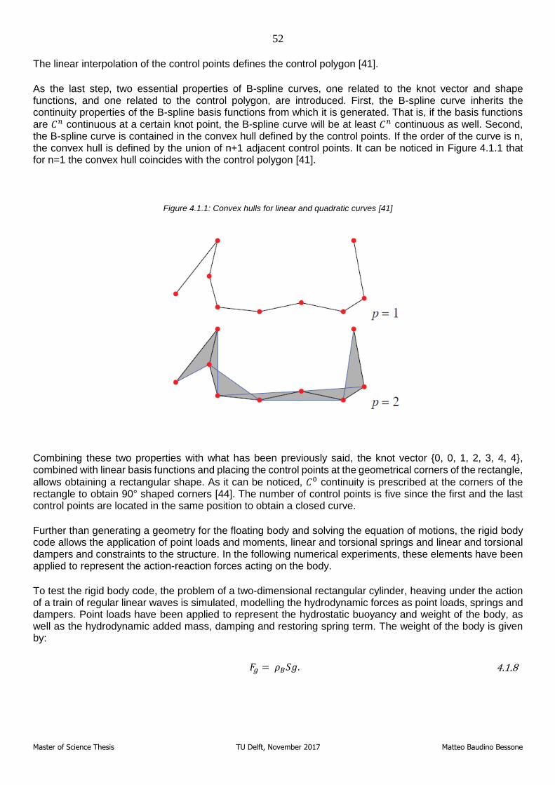
52


The linear interpolation of the control points defines the control polygon [41].

As the last step, two essential properties of B-spline curves, one related to the knot vector and shape functions, and one related to the control polygon, are introduced. First, the B-spline curve inherits the continuity properties of the B-spline basis functions from which it is generated. That is, if the basis functions are 𝐶𝑛 continuous at a certain knot point, the B-spline curve will be at least 𝐶𝑛 continuous as well. Second, the B-spline curve is contained in the convex hull defined by the control points. If the order of the curve is n, the convex hull is defined by the union of n+1 adjacent control points. It can be noticed in Figure 4.1.1 that for n=1 the convex hull coincides with the control polygon [41].

Figure 4.1.1: Convex hulls for linear and quadratic curves [41]

Combining these two properties with what has been previously said, the knot vector {0, 0, 1, 2, 3, 4, 4}, combined with linear basis functions and placing the control points at the geometrical corners of the rectangle,

allows obtaining a rectangular shape. As it can be noticed, 𝐶0 continuity is prescribed at the corners of the rectangle to obtain 90° shaped corners [44]. The number of control points is five since the first and the last control points are located in the same position to obtain a closed curve.

Further than generating a geometry for the floating body and solving the equation of motions, the rigid body code allows the application of point loads and moments, linear and torsional springs and linear and torsional dampers and constraints to the structure. In the following numerical experiments, these elements have been applied to represent the action-reaction forces acting on the body.

To test the rigid body code, the problem of a two-dimensional rectangular cylinder, heaving under the action of a train of regular linear waves is simulated, modelling the hydrodynamic forces as point loads, springs and dampers. Point loads have been applied to represent the hydrostatic buoyancy and weight of the body, as well as the hydrodynamic added mass, damping and restoring spring term. The weight of the body is given by:

𝐹𝑔 = 𝜌𝐵𝑆𝑔. 4.1.8

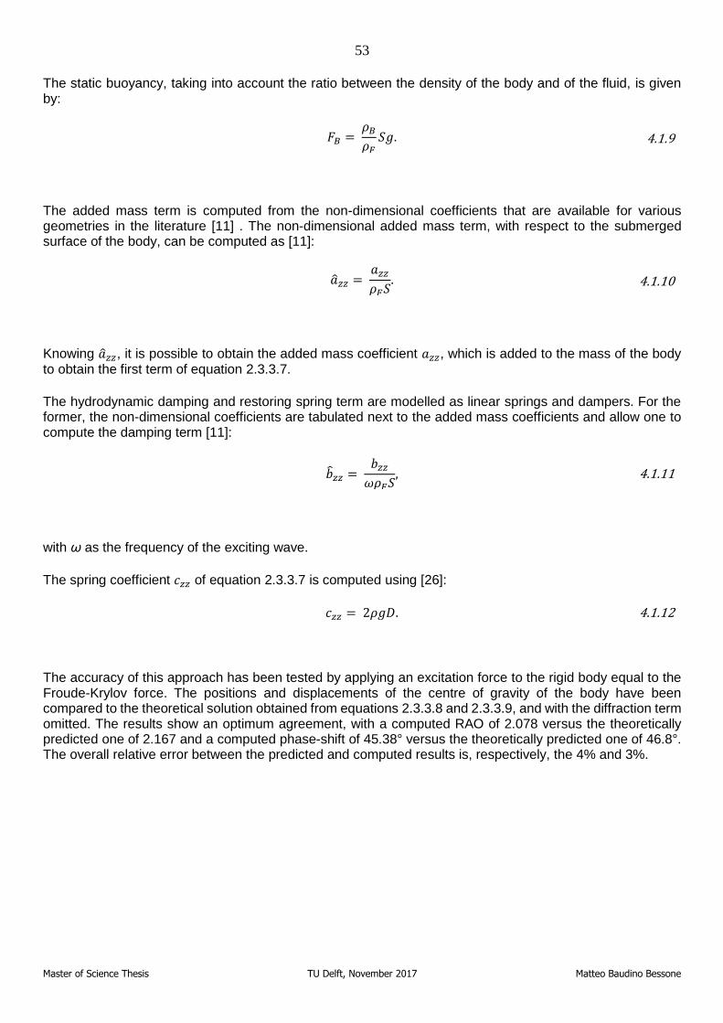
53


The static buoyancy, taking into account the ratio between the density of the body and of the fluid, is given by:

𝐹𝐵 = 𝜌𝐵𝜌𝐹𝑆𝑔. 4.1.9

The added mass term is computed from the non-dimensional coefficients that are available for various geometries in the literature [11] . The non-dimensional added mass term, with respect to the submerged surface of the body, can be computed as [11]:

�̂�𝑧𝑧 = 𝑎𝑧𝑧𝜌𝐹𝑆

. 4.1.10

Knowing �̂�𝑧𝑧, it is possible to obtain the added mass coefficient 𝑎𝑧𝑧, which is added to the mass of the body to obtain the first term of equation 2.3.3.7.

The hydrodynamic damping and restoring spring term are modelled as linear springs and dampers. For the former, the non-dimensional coefficients are tabulated next to the added mass coefficients and allow one to compute the damping term [11]:

�̂�𝑧𝑧 =

𝑏𝑧𝑧𝜔𝜌𝐹𝑆

, 4.1.11

with ω as the frequency of the exciting wave.

The spring coefficient 𝑐𝑧𝑧 of equation 2.3.3.7 is computed using [26]:

𝑐𝑧𝑧 = 2𝜌𝑔𝐷. 4.1.12

The accuracy of this approach has been tested by applying an excitation force to the rigid body equal to the Froude-Krylov force. The positions and displacements of the centre of gravity of the body have been compared to the theoretical solution obtained from equations 2.3.3.8 and 2.3.3.9, and with the diffraction term omitted. The results show an optimum agreement, with a computed RAO of 2.078 versus the theoretically predicted one of 2.167 and a computed phase-shift of 45.38° versus the theoretically predicted one of 46.8°. The overall relative error between the predicted and computed results is, respectively, the 4% and 3%.

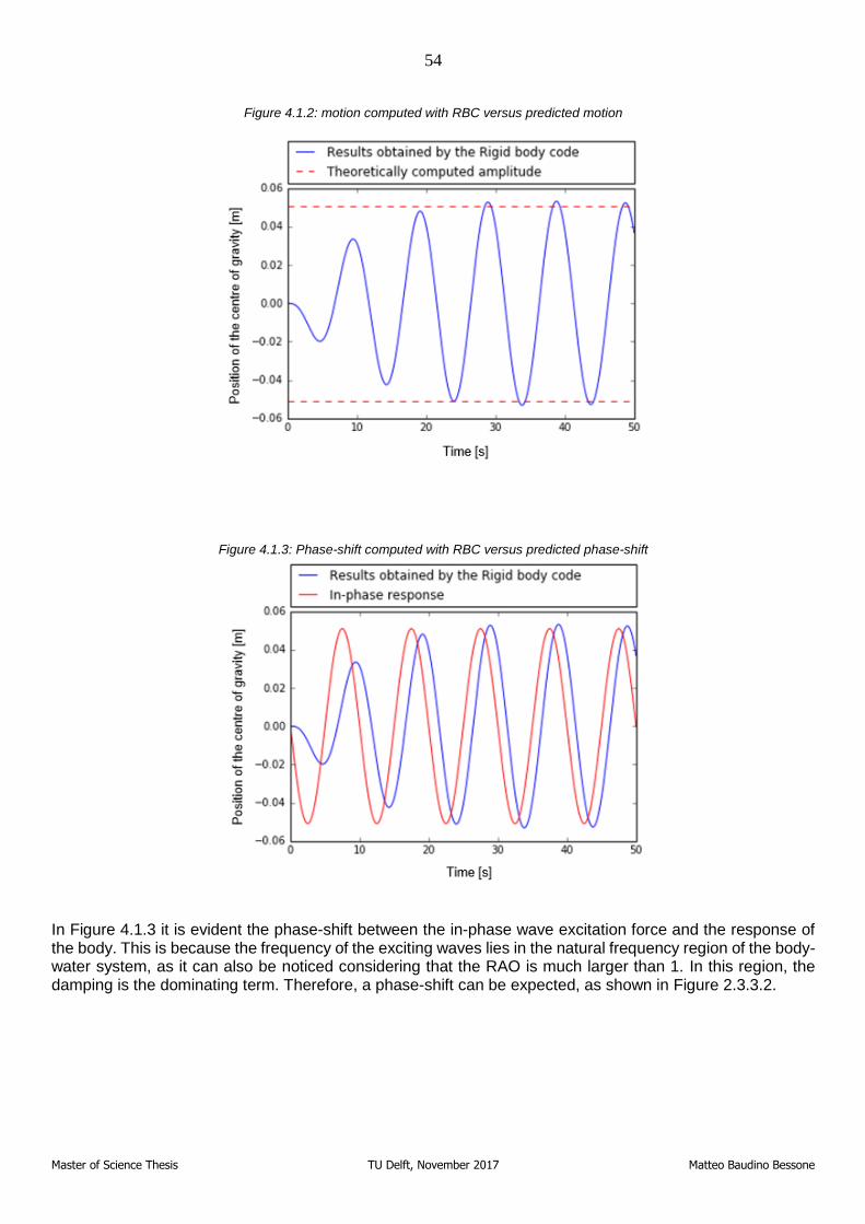
54


Figure 4.1.2: motion computed with RBC versus predicted motion

Figure 4.1.3: Phase-shift computed with RBC versus predicted phase-shift

In Figure 4.1.3 it is evident the phase-shift between the in-phase wave excitation force and the response of the body. This is because the frequency of the exciting waves lies in the natural frequency region of the body-water system, as it can also be noticed considering that the RAO is much larger than 1. In this region, the damping is the dominating term. Therefore, a phase-shift can be expected, as shown in Figure 2.3.3.2.

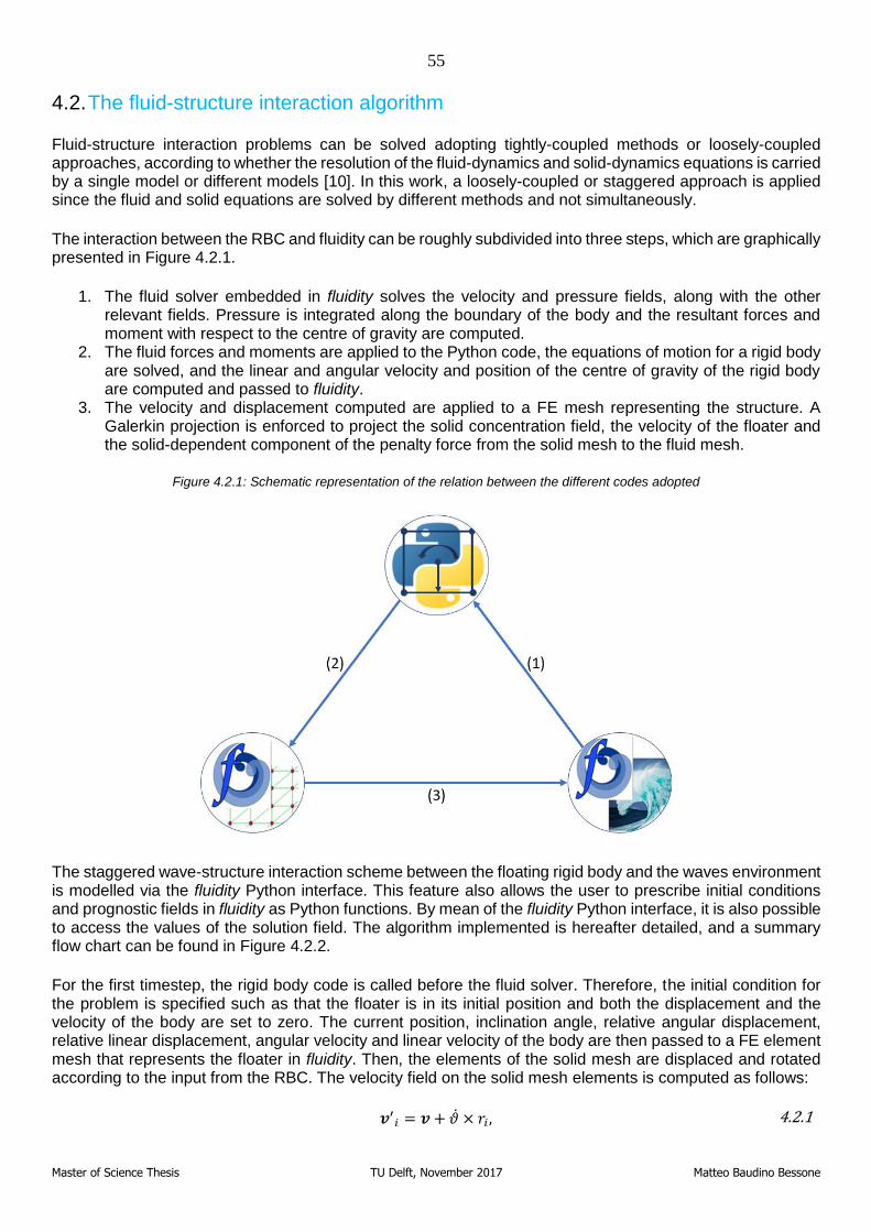
55


4.2. The fluid-structure interaction algorithm

Fluid-structure interaction problems can be solved adopting tightly-coupled methods or loosely-coupled approaches, according to whether the resolution of the fluid-dynamics and solid-dynamics equations is carried by a single model or different models [10]. In this work, a loosely-coupled or staggered approach is applied since the fluid and solid equations are solved by different methods and not simultaneously.

The interaction between the RBC and fluidity can be roughly subdivided into three steps, which are graphically presented in Figure 4.2.1.

1. The fluid solver embedded in fluidity solves the velocity and pressure fields, along with the other relevant fields. Pressure is integrated along the boundary of the body and the resultant forces and moment with respect to the centre of gravity are computed.

2. The fluid forces and moments are applied to the Python code, the equations of motion for a rigid body are solved, and the linear and angular velocity and position of the centre of gravity of the rigid body are computed and passed to fluidity.

3. The velocity and displacement computed are applied to a FE mesh representing the structure. A Galerkin projection is enforced to project the solid concentration field, the velocity of the floater and the solid-dependent component of the penalty force from the solid mesh to the fluid mesh.

Figure 4.2.1: Schematic representation of the relation between the different codes adopted

The staggered wave-structure interaction scheme between the floating rigid body and the waves environment is modelled via the fluidity Python interface. This feature also allows the user to prescribe initial conditions and prognostic fields in fluidity as Python functions. By mean of the fluidity Python interface, it is also possible to access the values of the solution field. The algorithm implemented is hereafter detailed, and a summary flow chart can be found in Figure 4.2.2.

For the first timestep, the rigid body code is called before the fluid solver. Therefore, the initial condition for the problem is specified such as that the floater is in its initial position and both the displacement and the velocity of the body are set to zero. The current position, inclination angle, relative angular displacement, relative linear displacement, angular velocity and linear velocity of the body are then passed to a FE element mesh that represents the floater in fluidity. Then, the elements of the solid mesh are displaced and rotated according to the input from the RBC. The velocity field on the solid mesh elements is computed as follows:

𝒗′𝑖 = 𝒗 + �̇� × 𝑟𝑖, 4.2.1

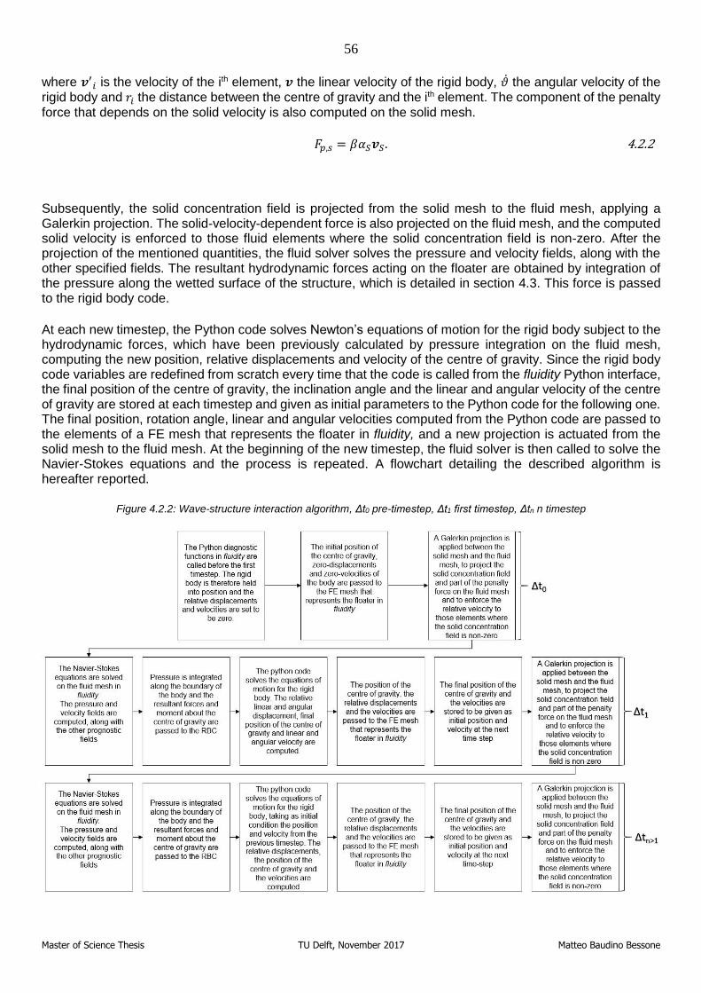
56


where 𝒗′𝑖 is the velocity of the ith element, 𝒗 the linear velocity of the rigid body, �̇� the angular velocity of the rigid body and 𝑟𝑖 the distance between the centre of gravity and the ith element. The component of the penalty force that depends on the solid velocity is also computed on the solid mesh.

𝐹𝑝,𝑠 = 𝛽𝛼𝑆𝒗𝑆. 4.2.2

Subsequently, the solid concentration field is projected from the solid mesh to the fluid mesh, applying a Galerkin projection. The solid-velocity-dependent force is also projected on the fluid mesh, and the computed solid velocity is enforced to those fluid elements where the solid concentration field is non-zero. After the projection of the mentioned quantities, the fluid solver solves the pressure and velocity fields, along with the other specified fields. The resultant hydrodynamic forces acting on the floater are obtained by integration of the pressure along the wetted surface of the structure, which is detailed in section 4.3. This force is passed to the rigid body code.

At each new timestep, the Python code solves Newton’s equations of motion for the rigid body subject to the hydrodynamic forces, which have been previously calculated by pressure integration on the fluid mesh, computing the new position, relative displacements and velocity of the centre of gravity. Since the rigid body code variables are redefined from scratch every time that the code is called from the fluidity Python interface, the final position of the centre of gravity, the inclination angle and the linear and angular velocity of the centre of gravity are stored at each timestep and given as initial parameters to the Python code for the following one. The final position, rotation angle, linear and angular velocities computed from the Python code are passed to the elements of a FE mesh that represents the floater in fluidity, and a new projection is actuated from the solid mesh to the fluid mesh. At the beginning of the new timestep, the fluid solver is then called to solve the Navier-Stokes equations and the process is repeated. A flowchart detailing the described algorithm is hereafter reported.

Figure 4.2.2: Wave-structure interaction algorithm, Δt0 pre-timestep, Δt1 first timestep, Δtn n timestep

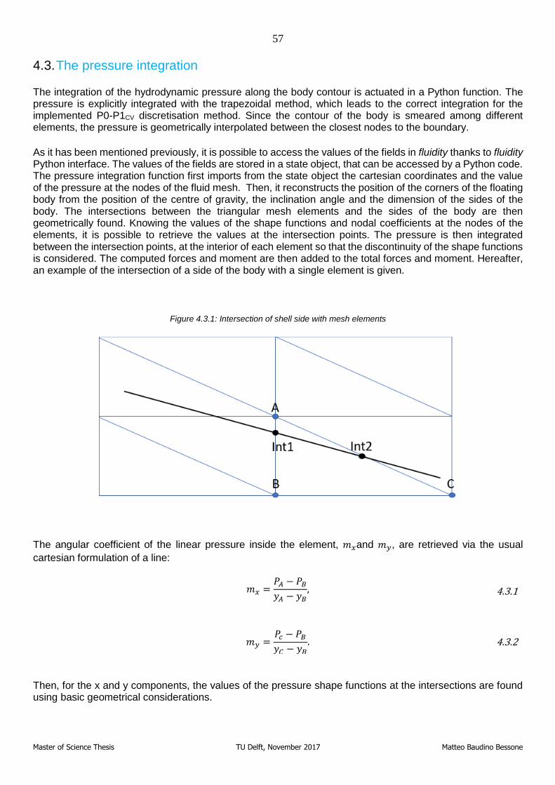
57


4.3. The pressure integration

The integration of the hydrodynamic pressure along the body contour is actuated in a Python function. The pressure is explicitly integrated with the trapezoidal method, which leads to the correct integration for the implemented P0-P1CV discretisation method. Since the contour of the body is smeared among different elements, the pressure is geometrically interpolated between the closest nodes to the boundary.

As it has been mentioned previously, it is possible to access the values of the fields in fluidity thanks to fluidity Python interface. The values of the fields are stored in a state object, that can be accessed by a Python code. The pressure integration function first imports from the state object the cartesian coordinates and the value of the pressure at the nodes of the fluid mesh. Then, it reconstructs the position of the corners of the floating body from the position of the centre of gravity, the inclination angle and the dimension of the sides of the body. The intersections between the triangular mesh elements and the sides of the body are then geometrically found. Knowing the values of the shape functions and nodal coefficients at the nodes of the elements, it is possible to retrieve the values at the intersection points. The pressure is then integrated between the intersection points, at the interior of each element so that the discontinuity of the shape functions is considered. The computed forces and moment are then added to the total forces and moment. Hereafter, an example of the intersection of a side of the body with a single element is given.

Figure 4.3.1: Intersection of shell side with mesh elements

The angular coefficient of the linear pressure inside the element, 𝑚𝑥and 𝑚𝑦, are retrieved via the usual

cartesian formulation of a line:

𝑚𝑥 =

𝑃𝐴 − 𝑃𝐵𝑦𝐴 − 𝑦𝐵

, 4.3.1

𝑚𝑦 =𝑃𝑐 − 𝑃𝐵𝑦𝐶 − 𝑦𝐵

. 4.3.2

Then, for the x and y components, the values of the pressure shape functions at the intersections are found using basic geometrical considerations.

58


{𝑝𝑖𝑛𝑡1𝑥 = 𝑝𝐴 +𝑚𝑥(𝑦𝑖𝑛𝑡1 − 𝑦𝐴),

𝑝𝑖𝑛𝑡2𝑥 = 𝑝𝐴 +𝑚𝑥(𝑦𝑖𝑛𝑡2 − 𝑦𝐴), 4.3.3

{𝑝𝑖𝑛𝑡1𝑦 = 𝑝𝐶 +𝑚𝑦(𝑥𝑖𝑛𝑡1 − 𝑥𝐶),

𝑝𝑖𝑛𝑡2𝑦 = 𝑝𝐶 +𝑚𝑦(𝑥𝑖𝑛𝑡2 − 𝑥𝐶). 4.3.4

The forces and moments acting on the section of the shell are then computed with the trapezoidal integration rule and added to the total forces and moments.

𝐹𝑥 = (

𝑝𝑖𝑛𝑡1𝑥 + 𝑝𝑖𝑛𝑡2𝑥2

) |𝑦𝑖𝑛𝑡1 − 𝑦𝑖𝑛𝑡2|𝑖,̂ 4.3.5

𝐹𝑦 = (

𝑝𝑖𝑛𝑡1𝑦 + 𝑝𝑖𝑛𝑡2𝑦

2) |𝑥 − 𝑥𝑖𝑛𝑡𝑦|𝑗̂, 4.3.6

𝑀𝑧 = [(

𝑥𝑖𝑛𝑡1 + 𝑥𝑖𝑛𝑡22

− 𝑋𝐶𝐺) , (𝑦𝑖𝑛𝑡1 + 𝑦𝑖𝑛𝑡2

2− 𝑌𝐶𝐺) , 0] × (𝐹𝑥 , 𝐹𝑦, 0), 4.3.7

where (𝑋𝐶𝐺 , 𝑌𝐶𝐺) is the position of the centre of gravity and 𝑖 ̂and 𝑗̂ unit normal vectors in longitudinal and vertical direction.

The accuracy of this approach was tested firstly on a simple hydrostatic case. A rigid body is immersed in a fluid at rest, and the hydrostatic force is computed on three different grids, whose parameters are reported in terms of PP side of the body in Table 4.3.1. The non-dimensional force is computed as follows:

𝐹𝑁𝐷 =

𝐹𝑓𝑙

𝐹𝑇ℎ𝑒𝑜, 4.3.8

in which 𝐹𝑁𝐷 is the non-dimensional force, 𝐹𝑓𝑙 is the force computed with fluidity and 𝐹𝑇ℎ𝑒𝑜 is the theoretical

force.

Table 4.3.1: Mesh parameters for hydrostatic validation pressure integration

Parameter Coarse mesh Intermediate

mesh Fine mesh

PP side of the body 26 33 44

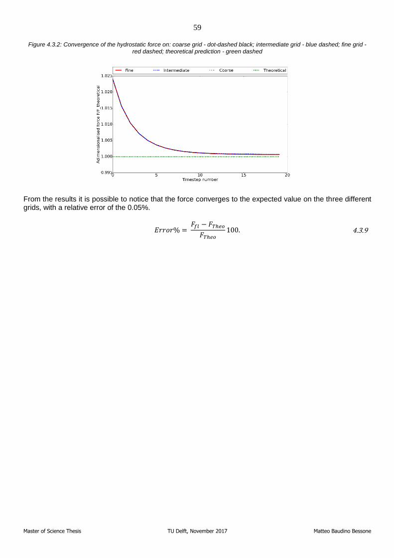
59


Figure 4.3.2: Convergence of the hydrostatic force on: coarse grid - dot-dashed black; intermediate grid - blue dashed; fine grid - red dashed; theoretical prediction - green dashed

From the results it is possible to notice that the force converges to the expected value on the three different grids, with a relative error of the 0.05%.

𝐸𝑟𝑟𝑜𝑟% =

𝐹𝑓𝑙 − 𝐹𝑇ℎ𝑒𝑜

𝐹𝑇ℎ𝑒𝑜100. 4.3.9

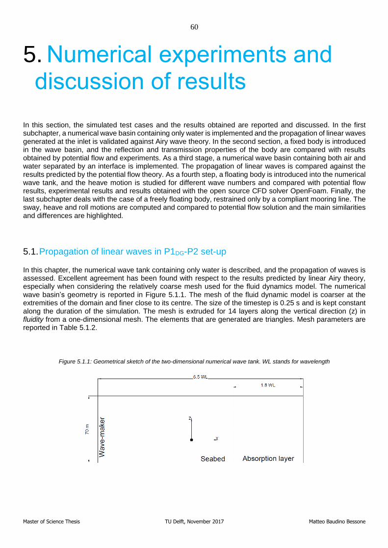
60


5. Numerical experiments and discussion of results

In this section, the simulated test cases and the results obtained are reported and discussed. In the first subchapter, a numerical wave basin containing only water is implemented and the propagation of linear waves generated at the inlet is validated against Airy wave theory. In the second section, a fixed body is introduced in the wave basin, and the reflection and transmission properties of the body are compared with results obtained by potential flow and experiments. As a third stage, a numerical wave basin containing both air and water separated by an interface is implemented. The propagation of linear waves is compared against the results predicted by the potential flow theory. As a fourth step, a floating body is introduced into the numerical wave tank, and the heave motion is studied for different wave numbers and compared with potential flow results, experimental results and results obtained with the open source CFD solver OpenFoam. Finally, the last subchapter deals with the case of a freely floating body, restrained only by a compliant mooring line. The sway, heave and roll motions are computed and compared to potential flow solution and the main similarities and differences are highlighted.

5.1. Propagation of linear waves in P1DG-P2 set-up

In this chapter, the numerical wave tank containing only water is described, and the propagation of waves is assessed. Excellent agreement has been found with respect to the results predicted by linear Airy theory, especially when considering the relatively coarse mesh used for the fluid dynamics model. The numerical wave basin’s geometry is reported in Figure 5.1.1. The mesh of the fluid dynamic model is coarser at the extremities of the domain and finer close to its centre. The size of the timestep is 0.25 s and is kept constant along the duration of the simulation. The mesh is extruded for 14 layers along the vertical direction (z) in fluidity from a one-dimensional mesh. The elements that are generated are triangles. Mesh parameters are reported in Table 5.1.2.

Figure 5.1.1: Geometrical sketch of the two-dimensional numerical wave tank. WL stands for wavelength

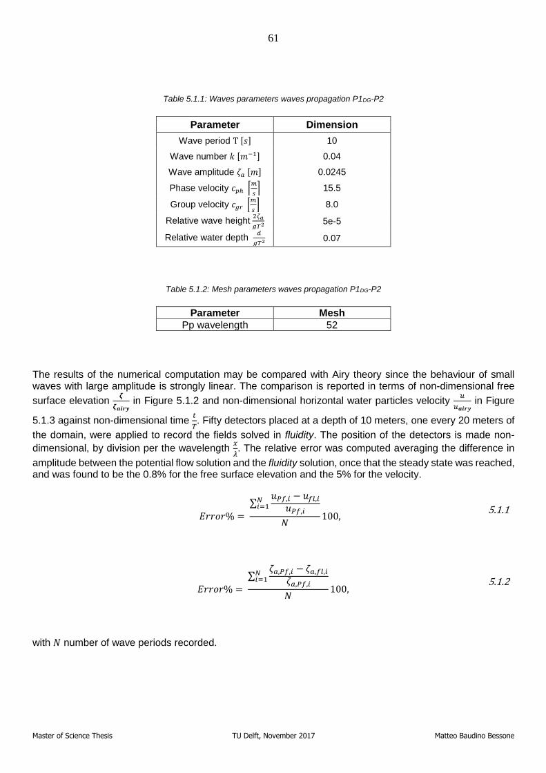
61


Table 5.1.1: Waves parameters waves propagation P1DG-P2

Parameter Dimension

Wave period T [𝑠] 10

Wave number 𝑘 [𝑚−1] 0.04

Wave amplitude 𝜁𝑎 [𝑚] 0.0245

Phase velocity 𝑐𝑝ℎ [𝑚

𝑠] 15.5

Group velocity 𝑐𝑔𝑟 [𝑚

𝑠] 8.0

Relative wave height 2𝜁𝑎

𝑔𝑇2 5e-5

Relative water depth 𝑑

𝑔𝑇2 0.07

Table 5.1.2: Mesh parameters waves propagation P1DG-P2

Parameter Mesh

Pp wavelength 52

The results of the numerical computation may be compared with Airy theory since the behaviour of small waves with large amplitude is strongly linear. The comparison is reported in terms of non-dimensional free

surface elevation 𝜻

𝜻𝒂𝒊𝒓𝒚 in Figure 5.1.2 and non-dimensional horizontal water particles velocity

𝑢

𝑢𝒂𝒊𝒓𝒚 in Figure

5.1.3 against non-dimensional time 𝑡

𝑇. Fifty detectors placed at a depth of 10 meters, one every 20 meters of

the domain, were applied to record the fields solved in fluidity. The position of the detectors is made non-

dimensional, by division per the wavelength 𝑥

𝜆. The relative error was computed averaging the difference in

amplitude between the potential flow solution and the fluidity solution, once that the steady state was reached, and was found to be the 0.8% for the free surface elevation and the 5% for the velocity.


∑𝑢𝑃𝑓,𝑖 − 𝑢𝑓𝑙,𝑖

𝑢𝑃𝑓,𝑖𝑁𝑖=1

𝑁100,

5.1.1


∑𝜁𝑎,𝑃𝑓,𝑖 − 𝜁𝑎,𝑓𝑙,𝑖

𝜁𝑎,𝑃𝑓,𝑖𝑁𝑖=1

𝑁100,

5.1.2

with 𝑁 number of wave periods recorded.

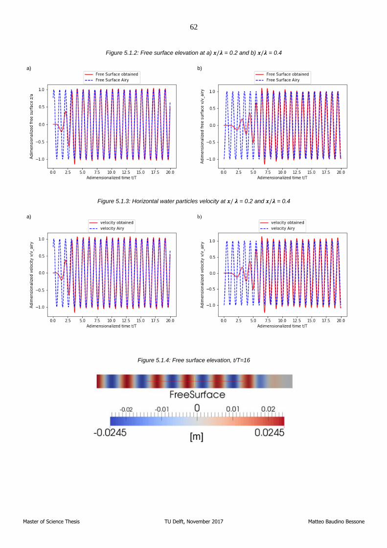
62


Figure 5.1.2: Free surface elevation at a) 𝒙/𝝀 = 0.2 and b) 𝒙/𝝀 = 0.4

a)

b)

Figure 5.1.3: Horizontal water particles velocity at 𝒙/ 𝝀 = 0.2 and 𝒙/𝝀 = 0.4

a)

b)

Figure 5.1.4: Free surface elevation, t/T=16

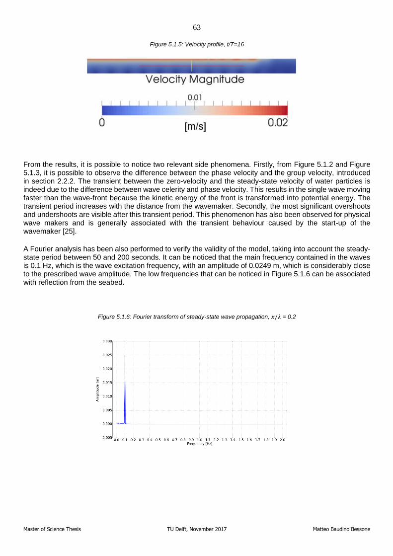
63


Figure 5.1.5: Velocity profile, t/T=16

From the results, it is possible to notice two relevant side phenomena. Firstly, from Figure 5.1.2 and Figure 5.1.3, it is possible to observe the difference between the phase velocity and the group velocity, introduced in section 2.2.2. The transient between the zero-velocity and the steady-state velocity of water particles is indeed due to the difference between wave celerity and phase velocity. This results in the single wave moving faster than the wave-front because the kinetic energy of the front is transformed into potential energy. The transient period increases with the distance from the wavemaker. Secondly, the most significant overshoots and undershoots are visible after this transient period. This phenomenon has also been observed for physical wave makers and is generally associated with the transient behaviour caused by the start-up of the wavemaker [25].

A Fourier analysis has been also performed to verify the validity of the model, taking into account the steady-state period between 50 and 200 seconds. It can be noticed that the main frequency contained in the waves is 0.1 Hz, which is the wave excitation frequency, with an amplitude of 0.0249 m, which is considerably close to the prescribed wave amplitude. The low frequencies that can be noticed in Figure 5.1.6 can be associated with reflection from the seabed.

Figure 5.1.6: Fourier transform of steady-state wave propagation, 𝒙/𝝀 = 0.2

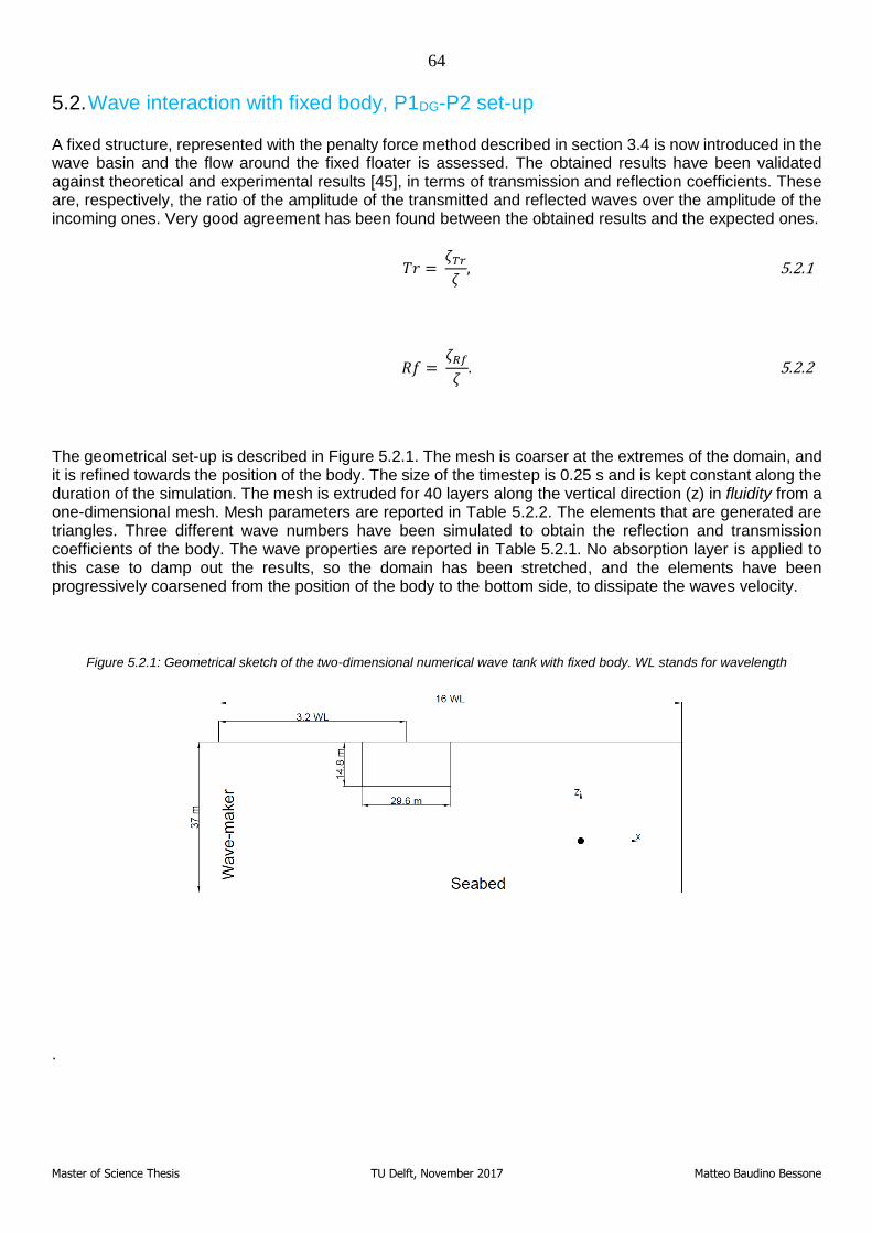
64


5.2. Wave interaction with fixed body, P1DG-P2 set-up

A fixed structure, represented with the penalty force method described in section 3.4 is now introduced in the wave basin and the flow around the fixed floater is assessed. The obtained results have been validated against theoretical and experimental results [45], in terms of transmission and reflection coefficients. These are, respectively, the ratio of the amplitude of the transmitted and reflected waves over the amplitude of the incoming ones. Very good agreement has been found between the obtained results and the expected ones.

𝑇𝑟 =

𝜁𝑇𝑟𝜁, 5.2.1

𝑅𝑓 =

𝜁𝑅𝑓

𝜁. 5.2.2

The geometrical set-up is described in Figure 5.2.1. The mesh is coarser at the extremes of the domain, and it is refined towards the position of the body. The size of the timestep is 0.25 s and is kept constant along the duration of the simulation. The mesh is extruded for 40 layers along the vertical direction (z) in fluidity from a one-dimensional mesh. Mesh parameters are reported in Table 5.2.2. The elements that are generated are triangles. Three different wave numbers have been simulated to obtain the reflection and transmission coefficients of the body. The wave properties are reported in Table 5.2.1. No absorption layer is applied to this case to damp out the results, so the domain has been stretched, and the elements have been progressively coarsened from the position of the body to the bottom side, to dissipate the waves velocity.

Figure 5.2.1: Geometrical sketch of the two-dimensional numerical wave tank with fixed body. WL stands for wavelength

.

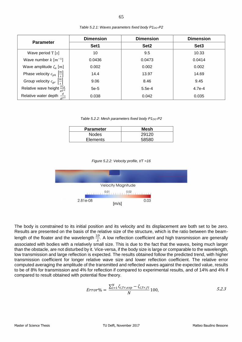
65


Table 5.2.1: Waves parameters fixed body P1DG-P2

Parameter Dimension Dimension Dimension

Set1 Set2 Set3

Wave period T [𝑠] 10 9.5 10.33

Wave number 𝑘 [𝑚−1] 0.0436 0.0473 0.0414

Wave amplitude 𝜁𝑎 [𝑚] 0.002 0.002 0.002


𝑠] 14.4 13.97 14.69


𝑠] 9.06 8.46 9.45


𝑔𝑇2 5e-5 5.5e-4 4.7e-4


𝑔𝑇2 0.038 0.042 0.035

Table 5.2.2: Mesh parameters fixed body P1DG-P2

Parameter Mesh

Nodes 29120 Elements 58580

Figure 5.2.2: Velocity profile, t/T =16

The body is constrained to its initial position and its velocity and its displacement are both set to be zero. Results are presented on the basis of the relative size of the structure, which is the ratio between the beam-

length of the floater and the wavelength 2𝐷

𝜆. A low reflection coefficient and high transmission are generally

associated with bodies with a relatively small size. This is due to the fact that the waves, being much larger than the obstacle, are not disturbed by it. Vice-versa, if the body size is large or comparable to the wavelength, low transmission and large reflection is expected. The results obtained follow the predicted trend, with higher transmission coefficient for longer relative wave size and lower reflection coefficient. The relative error computed averaging the amplitude of the transmitted and reflected waves against the expected value, results to be of 8% for transmission and 4% for reflection if compared to experimental results, and of 14% and 4% if compared to result obtained with potential flow theory.


∑ 𝜁𝑖,𝑇𝑟,𝑒𝑥𝑝 − 𝜁𝑖,𝑇𝑟,𝑓𝑙𝑁𝑖=1

𝑁100, 5.2.3

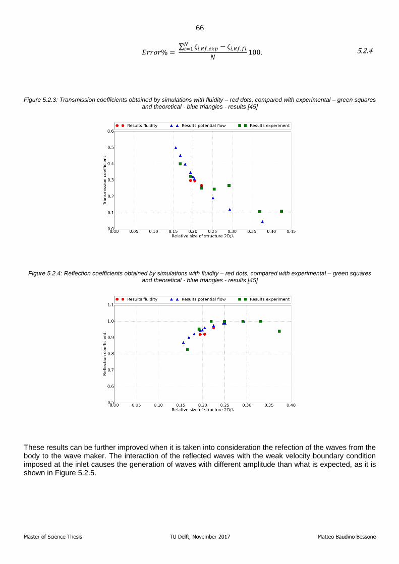
66



∑ 𝜁𝑖,𝑅𝑓,𝑒𝑥𝑝 − 𝜁𝑖,𝑅𝑓,𝑓𝑙𝑁𝑖=1

𝑁100. 5.2.4

Figure 5.2.3: Transmission coefficients obtained by simulations with fluidity – red dots, compared with experimental – green squares

and theoretical - blue triangles - results [45]

Figure 5.2.4: Reflection coefficients obtained by simulations with fluidity – red dots, compared with experimental – green squares

and theoretical - blue triangles - results [45]

These results can be further improved when it is taken into consideration the refection of the waves from the body to the wave maker. The interaction of the reflected waves with the weak velocity boundary condition imposed at the inlet causes the generation of waves with different amplitude than what is expected, as it is shown in Figure 5.2.5.

67


Figure 5.2.5: Time series of wave amplitude recorded at the wave maker, 𝒙/𝝀 =0

It is evident that the weakly imposed boundary condition at the inlet is affected by the reflection from the body. The amplitude of the waves generated is consistent with the prescription up to nearly 7 periods, then the effect of the reflected waves causes a deviation from the imposed wave properties.

To avoid this problem, the time that is necessary for the waves to travel back and forth from the body can be computed from the phase velocity. This allows finding a time window where the waves generated by the wavemaker are not affected by the reflection of the body. If only these results are taken into account, the agreement with experimental results and theory is at its maximum, generating a maximum relative error of the 2.8% for the transmission and of the 1.5% for the reflection with respect to experimental results, and, respectively, 11% and 1.6% if compared to theory.

Figure 5.2.6: Transmission coefficients obtained by simulations with fluidity, – red dots, taking into account the waves not polluted by the reflection to the wavemaker, compared with experimental – green squares and theoretical - blue triangles results [45]

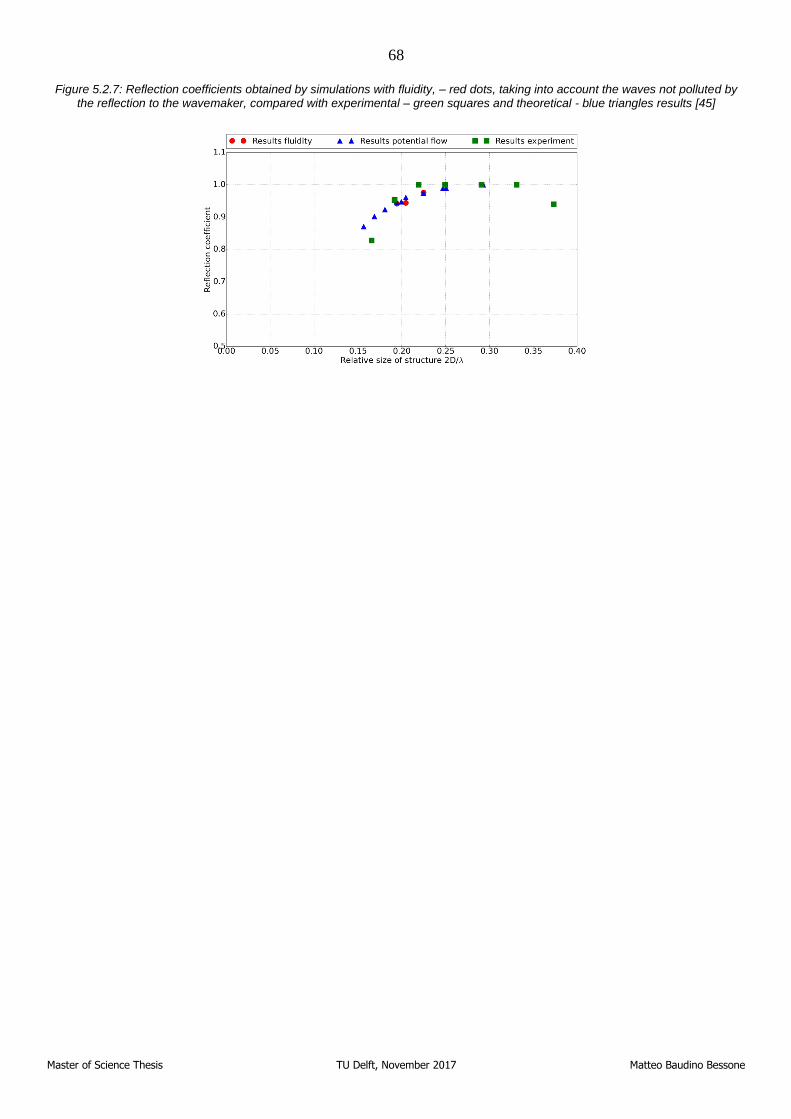
68


Figure 5.2.7: Reflection coefficients obtained by simulations with fluidity, – red dots, taking into account the waves not polluted by the reflection to the wavemaker, compared with experimental – green squares and theoretical - blue triangles results [45]

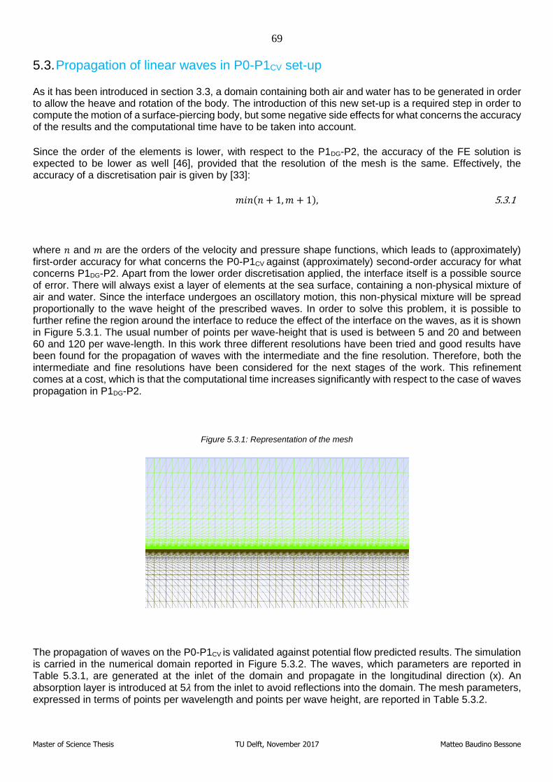
69


5.3. Propagation of linear waves in P0-P1CV set-up

As it has been introduced in section 3.3, a domain containing both air and water has to be generated in order to allow the heave and rotation of the body. The introduction of this new set-up is a required step in order to compute the motion of a surface-piercing body, but some negative side effects for what concerns the accuracy of the results and the computational time have to be taken into account.

Since the order of the elements is lower, with respect to the P1DG-P2, the accuracy of the FE solution is expected to be lower as well [46], provided that the resolution of the mesh is the same. Effectively, the accuracy of a discretisation pair is given by [33]:

𝑚𝑖𝑛(𝑛 + 1,𝑚 + 1), 5.3.1

where 𝑛 and 𝑚 are the orders of the velocity and pressure shape functions, which leads to (approximately) first-order accuracy for what concerns the P0-P1CV against (approximately) second-order accuracy for what concerns P1DG-P2. Apart from the lower order discretisation applied, the interface itself is a possible source of error. There will always exist a layer of elements at the sea surface, containing a non-physical mixture of air and water. Since the interface undergoes an oscillatory motion, this non-physical mixture will be spread proportionally to the wave height of the prescribed waves. In order to solve this problem, it is possible to further refine the region around the interface to reduce the effect of the interface on the waves, as it is shown in Figure 5.3.1. The usual number of points per wave-height that is used is between 5 and 20 and between 60 and 120 per wave-length. In this work three different resolutions have been tried and good results have been found for the propagation of waves with the intermediate and the fine resolution. Therefore, both the intermediate and fine resolutions have been considered for the next stages of the work. This refinement comes at a cost, which is that the computational time increases significantly with respect to the case of waves propagation in P1DG-P2.

Figure 5.3.1: Representation of the mesh

The propagation of waves on the P0-P1CV is validated against potential flow predicted results. The simulation is carried in the numerical domain reported in Figure 5.3.2. The waves, which parameters are reported in Table 5.3.1, are generated at the inlet of the domain and propagate in the longitudinal direction (x). An absorption layer is introduced at 5𝜆 from the inlet to avoid reflections into the domain. The mesh parameters, expressed in terms of points per wavelength and points per wave height, are reported in Table 5.3.2.

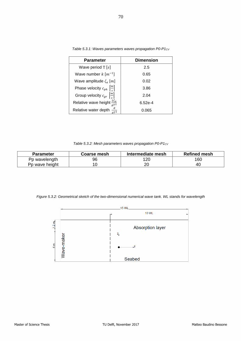
70


Table 5.3.1: Waves parameters waves propagation P0-P1CV

Parameter Dimension

Wave period T [𝑠] 2.5




𝑠] 3.86


𝑠] 2.04


𝑔𝑇2 6.52e-4


𝑔𝑇2 0.065

Table 5.3.2: Mesh parameters waves propagation P0-P1CV

Parameter Coarse mesh Intermediate mesh Refined mesh

Pp wavelength 96 120 160 Pp wave height 10 20 40

Figure 5.3.2: Geometrical sketch of the two-dimensional numerical wave tank. WL stands for wavelength

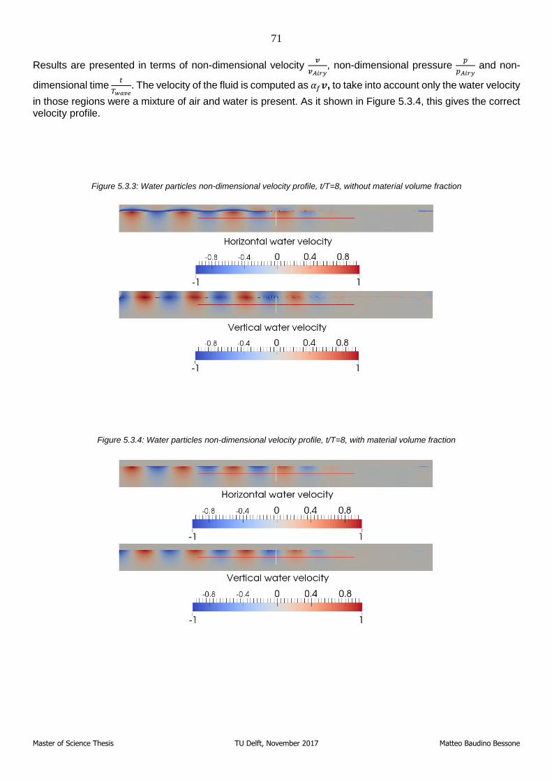
71


Results are presented in terms of non-dimensional velocity 𝒗

𝒗𝐴𝑖𝑟𝑦, non-dimensional pressure

𝑝

𝑝𝐴𝑖𝑟𝑦 and non-

dimensional time 𝑡

𝑇𝑤𝑎𝑣𝑒. The velocity of the fluid is computed as 𝛼𝑓𝒗, to take into account only the water velocity

in those regions were a mixture of air and water is present. As it shown in Figure 5.3.4, this gives the correct velocity profile.

Figure 5.3.3: Water particles non-dimensional velocity profile, t/T=8, without material volume fraction

Figure 5.3.4: Water particles non-dimensional velocity profile, t/T=8, with material volume fraction

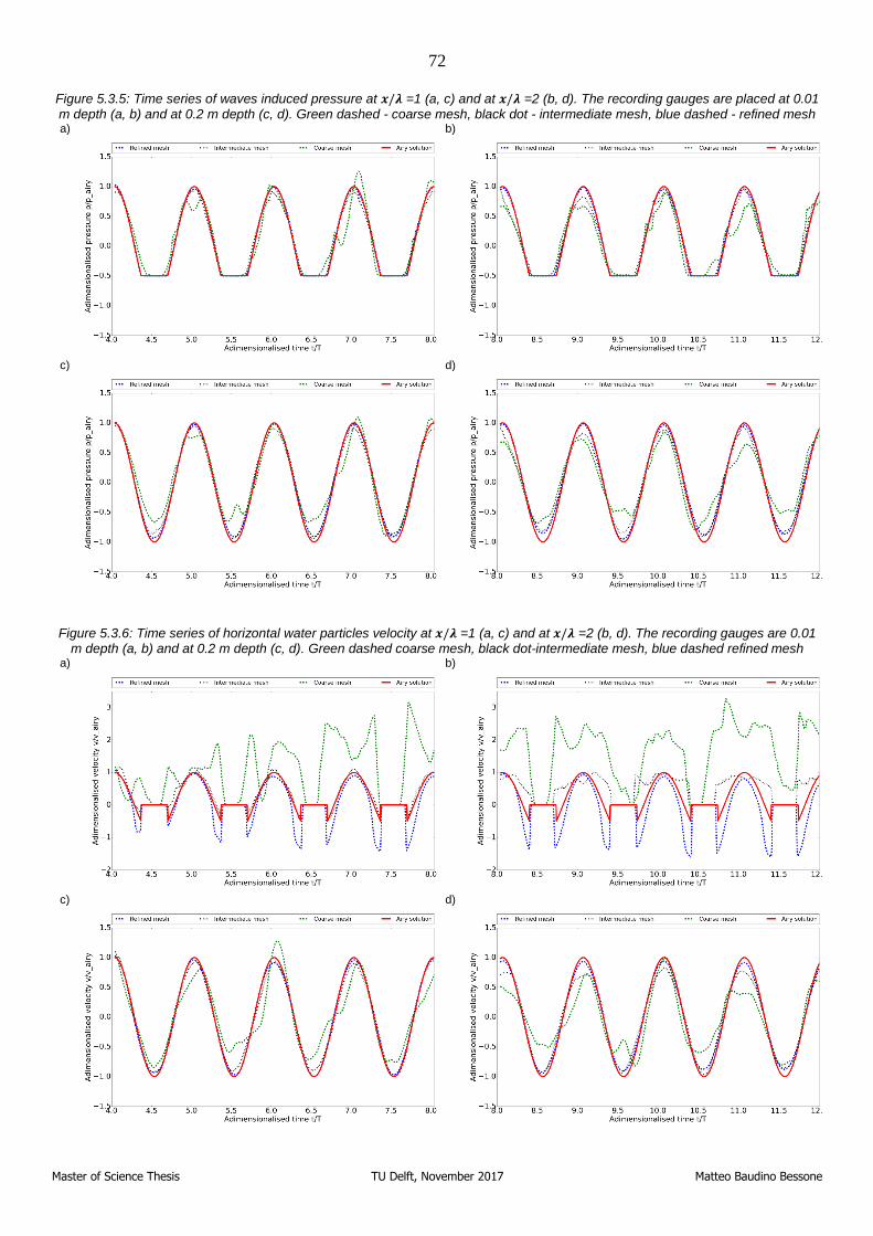
72


Figure 5.3.5: Time series of waves induced pressure at 𝒙/𝝀 =1 (a, c) and at 𝒙/𝝀 =2 (b, d). The recording gauges are placed at 0.01 m depth (a, b) and at 0.2 m depth (c, d). Green dashed - coarse mesh, black dot - intermediate mesh, blue dashed - refined mesh a)

b)

c)

d)

Figure 5.3.6: Time series of horizontal water particles velocity at 𝒙/𝝀 =1 (a, c) and at 𝒙/𝝀 =2 (b, d). The recording gauges are 0.01 m depth (a, b) and at 0.2 m depth (c, d). Green dashed coarse mesh, black dot-intermediate mesh, blue dashed refined mesh

a)

b)

c)

d)

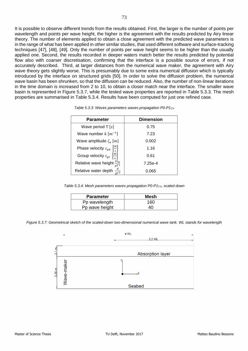
73


It is possible to observe different trends from the results obtained. First, the larger is the number of points per wavelength and points per wave height, the higher is the agreement with the results predicted by Airy linear theory. The number of elements applied to obtain a close agreement with the predicted wave parameters is in the range of what has been applied in other similar studies, that used different software and surface-tracking techniques [47], [48], [49]. Only the number of points per wave height seems to be higher than the usually applied one. Second, the results recorded in deeper waters match better the results predicted by potential flow also with coarser discretisation, confirming that the interface is a possible source of errors, if not accurately described. Third, at larger distances from the numerical wave maker, the agreement with Airy wave theory gets slightly worse. This is presumably due to some extra numerical diffusion which is typically introduced by the interface on structured grids [50]. In order to solve the diffusion problem, the numerical wave basin has been shrunken, so that the diffusion can be reduced. Also, the number of non-linear iterations in the time domain is increased from 2 to 10, to obtain a closer match near the interface. The smaller wave basin is represented in Figure 5.3.7, while the tested wave properties are reported in Table 5.3.3. The mesh properties are summarised in Table 5.3.4. Results have been computed for just one refined case.

Table 5.3.3: Waves parameters waves propagation P0-P1CV

Parameter Dimension

Wave period T [𝑠] 0.75




𝑠] 1.16


𝑠] 0.61


𝑔𝑇2 7.25e-4


𝑔𝑇2 0.065

Table 5.3.4: Mesh parameters waves propagation P0-P1CV, scaled down

Parameter Mesh

Pp wavelength 160 Pp wave height 40

Figure 5.3.7: Geometrical sketch of the scaled-down two-dimensional numerical wave tank. WL stands for wavelength

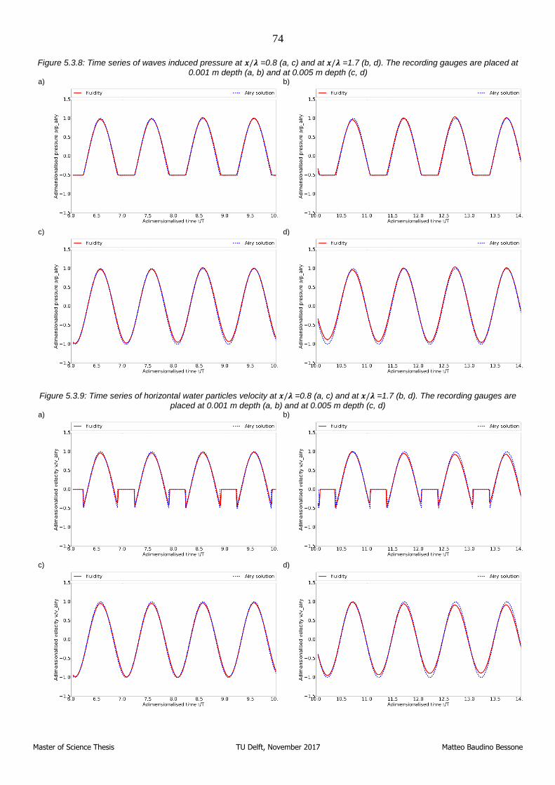
74


Figure 5.3.8: Time series of waves induced pressure at 𝒙/𝝀 =0.8 (a, c) and at 𝒙/𝝀 =1.7 (b, d). The recording gauges are placed at 0.001 m depth (a, b) and at 0.005 m depth (c, d)

a)

b)

c)

d)

Figure 5.3.9: Time series of horizontal water particles velocity at 𝒙/𝝀 =0.8 (a, c) and at 𝒙/𝝀 =1.7 (b, d). The recording gauges are

placed at 0.001 m depth (a, b) and at 0.005 m depth (c, d) a)

b)

c)

d)

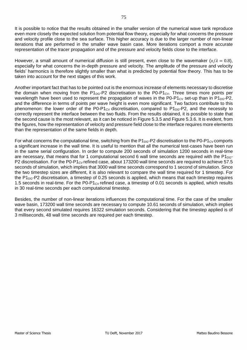
75


It is possible to notice that the results obtained in the smaller version of the numerical wave tank reproduce even more closely the expected solution from potential flow theory, especially for what concerns the pressure and velocity profile close to the sea surface. This higher accuracy is due to the larger number of non-linear iterations that are performed in the smaller wave basin case. More iterations comport a more accurate representation of the tracer propagation and of the pressure and velocity fields close to the interface.

However, a small amount of numerical diffusion is still present, even close to the wavemaker (𝑥/𝜆 = 0.8), especially for what concerns the in-depth pressure and velocity. The amplitude of the pressure and velocity fields’ harmonics is therefore slightly smaller than what is predicted by potential flow theory. This has to be taken into account for the next stages of this work.

Another important fact that has to be pointed out is the enormous increase of elements necessary to discretise the domain when moving from the P1DG-P2 discretisation to the P0-P1CV. Three times more points per wavelength have been used to represent the propagation of waves in the P0-P1CV set-up than in P1DG-P2, and the difference in terms of points per wave height is even more significant. Two factors contribute to this phenomenon: the lower order of the P0-P1CV discretisation, compared to P1DG-P2, and the necessity to correctly represent the interface between the two fluids. From the results obtained, it is possible to state that the second cause is the most relevant, as it can be noticed in Figure 5.3.5 and Figure 5.3.6. It is evident, from the figures, how the representation of velocity and pressure field close to the interface requires more elements than the representation of the same fields in depth.

For what concerns the computational time, switching from the P1DG-P2 discretisation to the P0-P1CV comports a significant increase in the wall time. It is useful to mention that all the numerical test-cases have been run in the same serial configuration. In order to compute 200 seconds of simulation 1200 seconds in real-time are necessary, that means that for 1 computational second 6 wall time seconds are required with the P1DG-P2 discretisation. For the P0-P1CV refined case, about 173200 wall time seconds are required to achieve 57.5 seconds of simulation, which implies that 3000 wall time seconds correspond to 1 second of simulation. Since the two timestep sizes are different, it is also relevant to compare the wall time required for 1 timestep. For the P1DG-P2 discretisation, a timestep of 0.25 seconds is applied, which means that each timestep requires 1.5 seconds in real-time. For the P0-P1CV refined case, a timestep of 0.01 seconds is applied, which results in 30 real-time seconds per each computational timestep.

Besides, the number of non-linear iterations influences the computational time. For the case of the smaller wave basin, 173200 wall time seconds are necessary to compute 10.61 seconds of simulation, which implies that every second simulated requires 16322 simulation seconds. Considering that the timestep applied is of 3 milliseconds, 48 wall time seconds are required per each timestep.

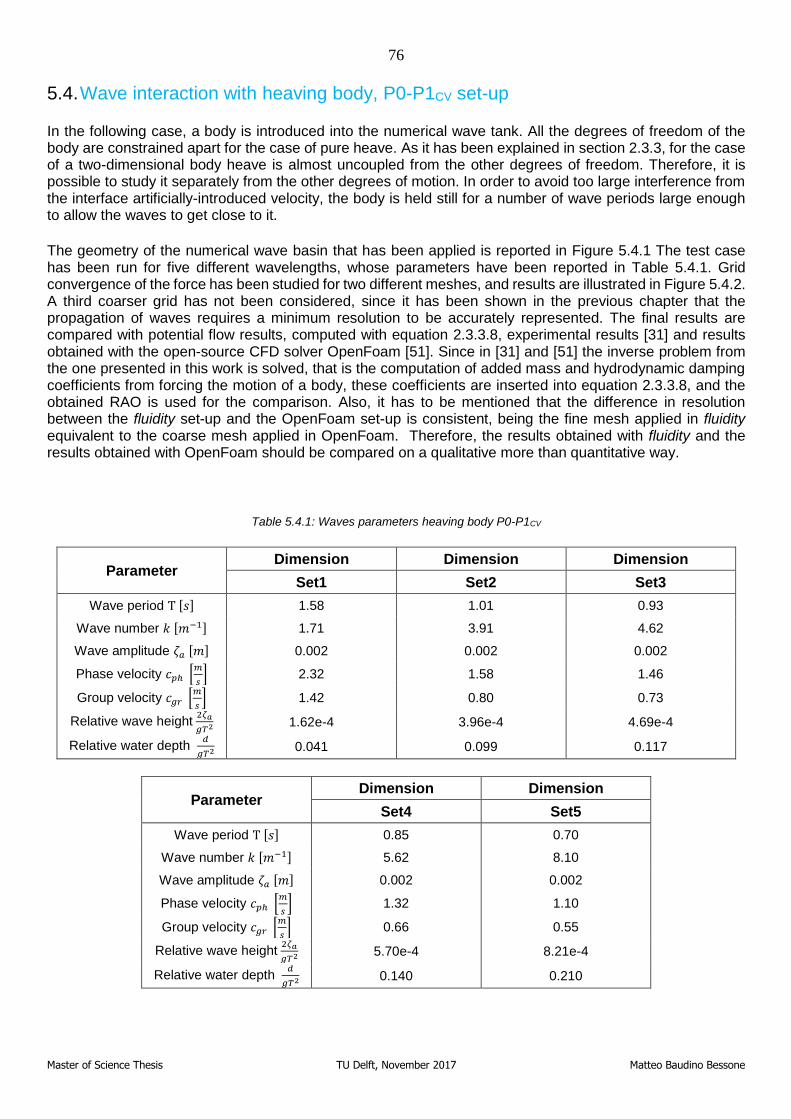
76


5.4. Wave interaction with heaving body, P0-P1CV set-up

In the following case, a body is introduced into the numerical wave tank. All the degrees of freedom of the body are constrained apart for the case of pure heave. As it has been explained in section 2.3.3, for the case of a two-dimensional body heave is almost uncoupled from the other degrees of freedom. Therefore, it is possible to study it separately from the other degrees of motion. In order to avoid too large interference from the interface artificially-introduced velocity, the body is held still for a number of wave periods large enough to allow the waves to get close to it.

The geometry of the numerical wave basin that has been applied is reported in Figure 5.4.1 The test case has been run for five different wavelengths, whose parameters have been reported in Table 5.4.1. Grid convergence of the force has been studied for two different meshes, and results are illustrated in Figure 5.4.2. A third coarser grid has not been considered, since it has been shown in the previous chapter that the propagation of waves requires a minimum resolution to be accurately represented. The final results are compared with potential flow results, computed with equation 2.3.3.8, experimental results [31] and results obtained with the open-source CFD solver OpenFoam [51]. Since in [31] and [51] the inverse problem from the one presented in this work is solved, that is the computation of added mass and hydrodynamic damping coefficients from forcing the motion of a body, these coefficients are inserted into equation 2.3.3.8, and the obtained RAO is used for the comparison. Also, it has to be mentioned that the difference in resolution between the fluidity set-up and the OpenFoam set-up is consistent, being the fine mesh applied in fluidity equivalent to the coarse mesh applied in OpenFoam. Therefore, the results obtained with fluidity and the results obtained with OpenFoam should be compared on a qualitative more than quantitative way.

Table 5.4.1: Waves parameters heaving body P0-P1CV

Parameter Dimension Dimension Dimension

Set1 Set2 Set3

Wave period T [𝑠] 1.58 1.01 0.93

Wave number 𝑘 [𝑚−1] 1.71 3.91 4.62

Wave amplitude 𝜁𝑎 [𝑚] 0.002 0.002 0.002


𝑠] 2.32 1.58 1.46


𝑠] 1.42 0.80 0.73


𝑔𝑇2 1.62e-4 3.96e-4 4.69e-4


𝑔𝑇2 0.041 0.099 0.117

Parameter Dimension Dimension

Set4 Set5

Wave period T [𝑠] 0.85 0.70

Wave number 𝑘 [𝑚−1] 5.62 8.10

Wave amplitude 𝜁𝑎 [𝑚] 0.002 0.002


𝑠] 1.32 1.10


𝑠] 0.66 0.55


𝑔𝑇2 5.70e-4 8.21e-4


𝑔𝑇2 0.140 0.210

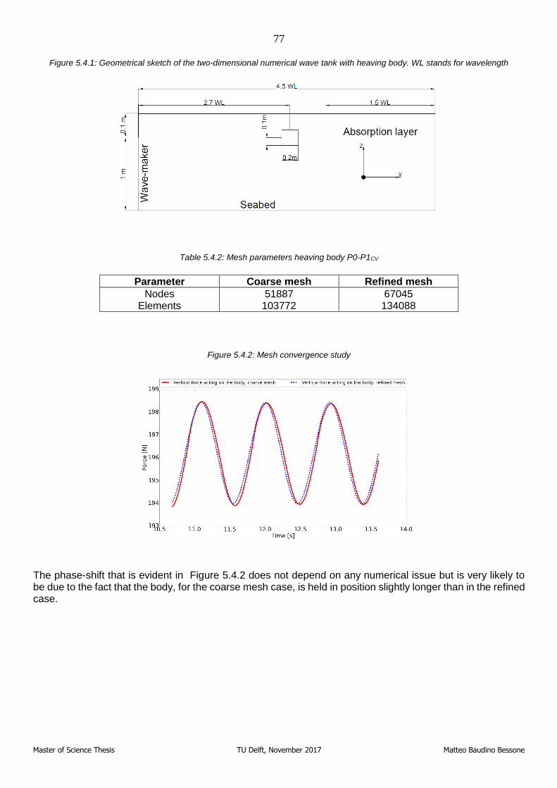
77


Figure 5.4.1: Geometrical sketch of the two-dimensional numerical wave tank with heaving body. WL stands for wavelength

Table 5.4.2: Mesh parameters heaving body P0-P1CV

Parameter Coarse mesh Refined mesh

Nodes 51887 67045 Elements 103772 134088

Figure 5.4.2: Mesh convergence study

The phase-shift that is evident in Figure 5.4.2 does not depend on any numerical issue but is very likely to be due to the fact that the body, for the coarse mesh case, is held in position slightly longer than in the refined case.

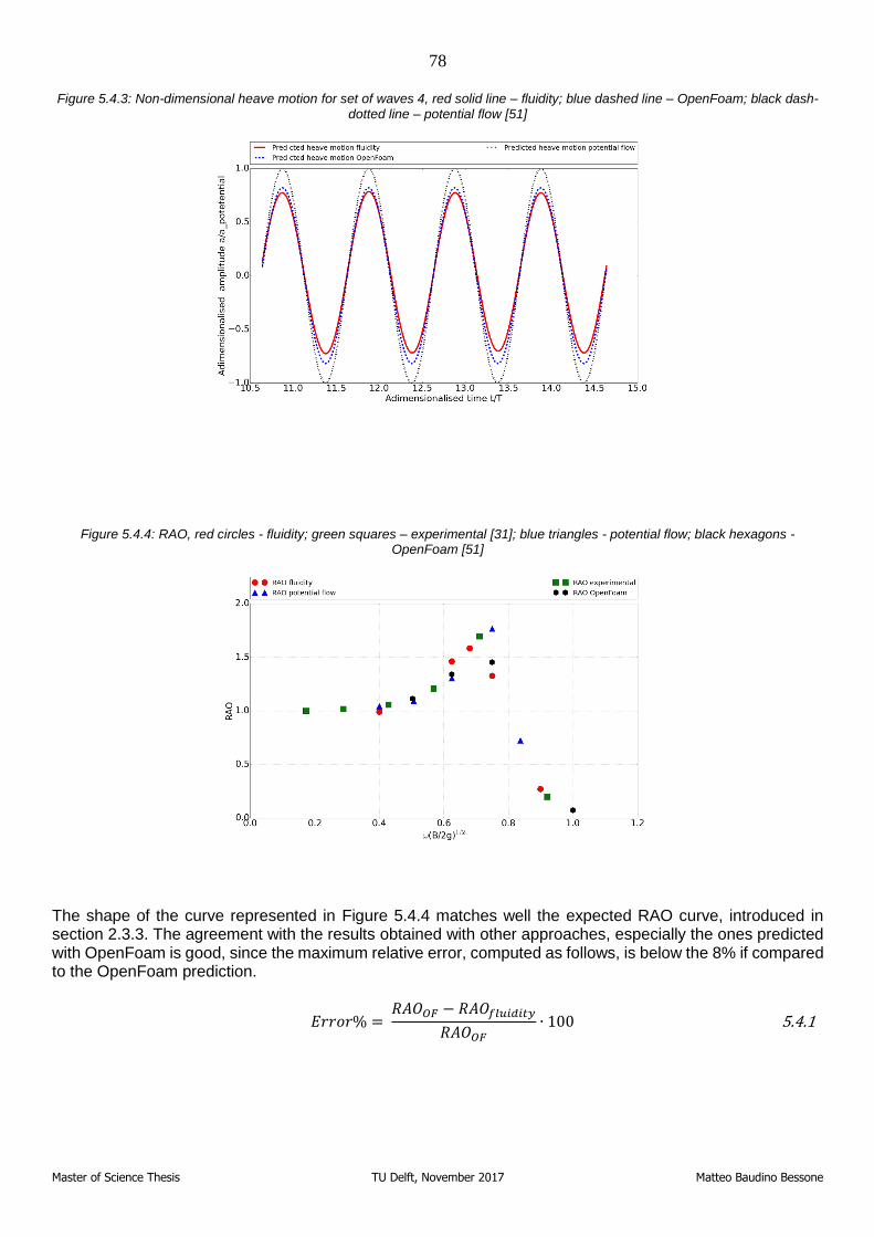
78


Figure 5.4.3: Non-dimensional heave motion for set of waves 4, red solid line – fluidity; blue dashed line – OpenFoam; black dash-dotted line – potential flow [51]

Figure 5.4.4: RAO, red circles - fluidity; green squares – experimental [31]; blue triangles - potential flow; black hexagons - OpenFoam [51]

The shape of the curve represented in Figure 5.4.4 matches well the expected RAO curve, introduced in section 2.3.3. The agreement with the results obtained with other approaches, especially the ones predicted with OpenFoam is good, since the maximum relative error, computed as follows, is below the 8% if compared to the OpenFoam prediction.


𝑅𝐴𝑂𝑂𝐹 − 𝑅𝐴𝑂𝑓𝑙𝑢𝑖𝑑𝑖𝑡𝑦

𝑅𝐴𝑂𝑂𝐹∙ 100 5.4.1

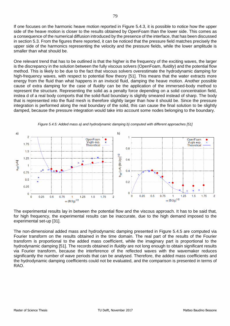
79


If one focuses on the harmonic heave motion reported in Figure 5.4.3, it is possible to notice how the upper side of the heave motion is closer to the results obtained by OpenFoam than the lower side. This comes as a consequence of the numerical diffusion introduced by the presence of the interface, that has been discussed in section 5.3. From the figures there reported, it can be noticed that the pressure field matches precisely the upper side of the harmonics representing the velocity and the pressure fields, while the lower amplitude is smaller than what should be.

One relevant trend that has to be outlined is that the higher is the frequency of the exciting waves, the larger is the discrepancy in the solution between the fully viscous solvers (OpenFoam, fluidity) and the potential flow method. This is likely to be due to the fact that viscous solvers overestimate the hydrodynamic damping for high-frequency waves, with respect to potential flow theory [51]. This means that the water extracts more energy from the fluid than what happens in an inviscid fluid, damping the heave motion. Another possible cause of extra damping for the case of fluidity can be the application of the immersed-body method to represent the structure. Representing the solid as a penalty force depending on a solid concentration field, instea d of a real body comports that the solid-fluid boundary is slightly smeared instead of sharp. The body that is represented into the fluid mesh is therefore slightly larger than how it should be. Since the pressure integration is performed along the real boundary of the solid, this can cause the final solution to be slightly damped, because the pressure integration would take into account some nodes belonging to the boundary.

Figure 5.4.5: Added mass a) and hydrodynamic damping b) computed with different approaches [51]

a)

b)

The experimental results lay in between the potential flow and the viscous approach. It has to be said that, for high frequency, the experimental results can be inaccurate, due to the high demand imposed to the experimental set-up [31].

The non-dimensional added mass and hydrodynamic damping presented in Figure 5.4.5 are computed via Fourier transform on the results obtained in the time domain. The real part of the results of the Fourier transform is proportional to the added mass coefficient, while the imaginary part is proportional to the hydrodynamic damping [51]. The records obtained in fluidity are not long enough to obtain significant results via Fourier transform, because the interference of the reflected waves with the wavemaker reduces significantly the number of wave periods that can be analysed. Therefore, the added mass coefficients and the hydrodynamic damping coefficients could not be evaluated, and the comparison is presented in terms of RAO.

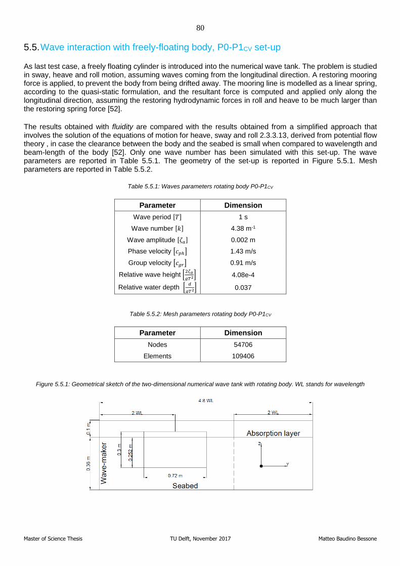
80


5.5. Wave interaction with freely-floating body, P0-P1CV set-up

As last test case, a freely floating cylinder is introduced into the numerical wave tank. The problem is studied in sway, heave and roll motion, assuming waves coming from the longitudinal direction. A restoring mooring force is applied, to prevent the body from being drifted away. The mooring line is modelled as a linear spring, according to the quasi-static formulation, and the resultant force is computed and applied only along the longitudinal direction, assuming the restoring hydrodynamic forces in roll and heave to be much larger than the restoring spring force [52].

The results obtained with fluidity are compared with the results obtained from a simplified approach that involves the solution of the equations of motion for heave, sway and roll 2.3.3.13, derived from potential flow theory , in case the clearance between the body and the seabed is small when compared to wavelength and beam-length of the body [52]. Only one wave number has been simulated with this set-up. The wave parameters are reported in Table 5.5.1. The geometry of the set-up is reported in Figure 5.5.1. Mesh parameters are reported in Table 5.5.2.

Table 5.5.1: Waves parameters rotating body P0-P1CV

Parameter Dimension

Wave period [𝑇] 1 s

Wave number [𝑘] 4.38 m-1

Wave amplitude [𝜁𝑎] 0.002 m

Phase velocity [𝑐𝑝ℎ] 1.43 m/s

Group velocity [𝑐𝑔𝑟] 0.91 m/s

Relative wave height [2𝜁𝑎

𝑔𝑇2] 4.08e-4

Relative water depth [𝑑

𝑔𝑇2] 0.037

Table 5.5.2: Mesh parameters rotating body P0-P1CV

Parameter Dimension

Nodes 54706

Elements 109406

Figure 5.5.1: Geometrical sketch of the two-dimensional numerical wave tank with rotating body. WL stands for wavelength

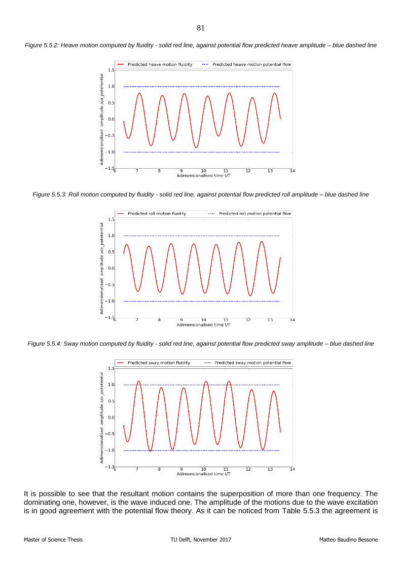
81


Figure 5.5.2: Heave motion computed by fluidity - solid red line, against potential flow predicted heave amplitude – blue dashed line

Figure 5.5.3: Roll motion computed by fluidity - solid red line, against potential flow predicted roll amplitude – blue dashed line

Figure 5.5.4: Sway motion computed by fluidity - solid red line, against potential flow predicted sway amplitude – blue dashed line

It is possible to see that the resultant motion contains the superposition of more than one frequency. The dominating one, however, is the wave induced one. The amplitude of the motions due to the wave excitation is in good agreement with the potential flow theory. As it can be noticed from Table 5.5.3 the agreement is

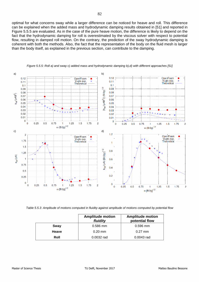
82


optimal for what concerns sway while a larger difference can be noticed for heave and roll. This difference can be explained when the added mass and hydrodynamic damping results obtained in [51] and reported in Figure 5.5.5 are evaluated. As in the case of the pure heave motion, the difference is likely to depend on the fact that the hydrodynamic damping for roll is overestimated by the viscous solver with respect to potential flow, resulting in damped roll motion. On the contrary, the prediction of the sway hydrodynamic damping is coherent with both the methods. Also, the fact that the representation of the body on the fluid mesh is larger than the body itself, as explained in the previous section, can contribute to the damping.

Figure 5.5.5: Roll a) and sway c) added mass and hydrodynamic damping b),d) with different approaches [51]

a)

b)

c)

d)

Table 5.5.3: Amplitude of motions computed in fluidity against amplitude of motions computed by potential flow

Amplitude motion

fluidity Amplitude motion

potential flow

Sway 0.586 mm 0.596 mm

Heave 0.20 mm 0.27 mm

Roll 0.0032 rad 0.0043 rad

83


The time-series of motion of the floater show the presence of frequencies lower than the wave excitation frequency. A Fourier analysis would be the best method to determine the effective amplitude and frequency of these responses, but the recordings are not long enough to allow to obtain meaningful results from the application of a Fourier transform. However, from the heave motion time series, it is possible to notice a low-frequency response with twice the period of the exciting waves. This matches with the heave natural period of the body, which has been computed as follows:

𝑇𝑧𝑁 =2𝜋

𝜔𝑧𝑁; 𝜔𝑁 = √

𝑐𝑧𝑧𝑚 + 𝑎𝑧𝑧

. 5.5.1

It is difficult to evidence the same correlation for the subharmonic frequency present in the sway and roll motion because the low-frequency excitation has a longer period. Therefore, a longer record of data would be necessary to assess whether those subharmonic frequencies match the sway and roll natural periods.

The cause of the subharmonic response of the body to wave excitation can be found in the reflections from the seabed to the floater. The potential flow theory against which this test-case has been validated was developed for pontoon-type breakwaters, in the limiting case that the clearance between the keel of the breakwater and the seabed is small with respect to the wavelength and draft of the breakwater [52]. Therefore, to match the potential flow condition, the numerical set-up has been adapted and the draft of the body has been increased. The small clearance enhances the interactions between the seabed and the floater, causing frequencies that can excite the natural periods of the system. This is evident when the heave motion introduced in this chapter are compared with the heave response of the previous heaving case, where the clearance between the keel and the seabed was large. No subharmonic response was found in that case.

84


6. Conclusions and recommendations

In this section, the most relevant findings and conclusions that have emerged during the development of this work are summarised. In the second subchapter, a short list of suggestions and recommendations for future work is given.

6.1. Conclusions

The capability of fluidity to represent regular linear waves’ propagation in two-dimensional (with one element extrusion) and three-dimensional numerical wave tanks, with P1DG-P2 discretisation, had already been assessed previously [6], [37]. In this work, a purely two-dimensional numerical wave basin is validated. Excellent agreement for what concerns free-surface elevation and velocity fields is found with respect to results predicted by potential flow theory.

Subsequently, the case of waves’ interaction with a fixed, rigid obstacle, represented with the immersed-body method, is assessed. Results are reported in terms of reflection and transmission coefficients, computed for three different wavelengths. The comparison is carried out taking into account experimental data and potential flow data available in the literature. An optimum agreement is found for both the cases, even if a slightly closer match is identified with the experimental results.

As a next step, the wave propagation in a two-dimensional numerical wave tank containing both air and water is computed and compared with the results predicted by linear Airy wave theory. The domain is spatially discretised with the P0-P1CV pair. The interface between air and water is represented by the volume of fluids method. It is found that to achieve an accuracy of results comparable to the P1DG-P2 case, the increase of elements applied for the discretisation is relevant. The causes of this escalation are mainly to be found in the necessity to bound the elements containing a non-physical mixture of air and water, introduced by the smeared interface, to a thin layer. The lower order of accuracy of the P0-P1CV pair with respect to the P1DG-P2 case is another cause of the increase of elements’ number. It is also reported that, reducing the dimensions of the wave basin and increasing the number of non-linear iterations in the time domain, the accuracy of the results increases. However, the amplitude of the pressure and velocity harmonics recorded in depth are found to be slightly smaller than the ones predicted by potential flow theory.

Finally, a loosely-coupled wave-structure interaction algorithm is implemented, and two different test-cases are simulated in the P0-P1CV wave basin. For the first case, a rigid body which degrees of freedom are restrained to heave motion is introduced in the numerical wave tank. The numerical experiments have been carried for five different wavelengths and compared with potential flow theory, experimental results and results obtained from the CFD solver OpenFoam. The results, evaluated in terms of RAO, match the expected shape of the curve. A good agreement is reached with the results obtained with OpenFoam, even if the resolution mesh implemented in fluidity is much coarser. With respect to potential flow, the agreement is good in the quasi-static region, but discrepancies are found close to resonance and in the region of the RAO curve dominated by the body motions. Three main reasons can be given to explain the differences. First, the amplitude of the velocity and pressure harmonics, which were discussed in the previous paragraph, is slightly lower than the one that is predicted by potential flow theory. Second, the application of the immersed-body method results in a slightly larger representation of the body in the fluid mesh, because the boundary of the body is smeared. Therefore, the integration of pressure is performed along the sharp boundary also takes

85


into account some points inside the body. Finally, it is likely that the application of a fully viscous solver comports the different estimation of the hydrodynamic damping and added mass coefficients with respect to potential flow theory. Mainly, the hydrodynamic damping is overestimated by viscous solvers with respect to potential flow theory. Experimental results lay in between the potential flow results and the results obtained with viscous solvers, and it is also mentioned that some experimental error is introduced at high wave frequency, due to the high stress imposed at high-frequencies. Further research is therefore needed to obtain experimental results to state how correct are the results obtained by viscous solvers at high frequencies.

In the second test-case, a rigid body free to move in sway, roll and heave is immersed in the numerical wave tank. A compliant mooring line is attached to the structure to prevent it from being drifted away. One single wavelength is simulated for this case. The results in term of the amplitude of motion are compared with the ones obtained with potential flow theory. The agreement for what concerns sway motion is very good, while the heave and roll amplitudes of motion are damped with respect to the results predicted by potential flow theory. This is again likely to be due to the fact that a viscous solver overestimates the hydrodynamic damping in heave and roll, while the prediction for what concerns sway motion matches well the one obtained with potential flow. In the rotating case, the presence of a frequency lower than the excitation wave frequency is observed. For the heave, this frequency matches well with the heave natural frequency of the water-body system. The cause of this excitation is presumably due to the stronger interaction body-seabed, which is a consequence of the extremely reduced clearance between the body and the seabed with respect to the pure heave case.

86


6.2. Recommendations

The present work is a good start point to develop a model to predict the motion of a floater for wind turbines in regular and irregular waves. Of course, to face complex problems the model has to be extended and improved, to include irregular wave generation, more complex geometries, accurate mooring lines modelling, and the effects of the wind turbine induced forces and moments on the floater, but the base to work on is already present, in terms of waves-structure interaction.

Under the consideration of implementing full-scale simulations, it can be interesting to implement the P1DG-P2 discretisation for the air-water model, to reduce the computational time and to increase the accuracy of the results. Since the multi-material volume approach that is implemented in fluidity right now requires finite volumes discretisation to ensure the boundedness of the material volume fraction, the implementation of an internal boundary condition representing the sea surface, which right now is not supported by fluidity, can be a way to bypass the necessity to use the multi-material model. The pressure integration function, then, should be extended to include the integration of quadratic shape functions.

Another approach that would be worthy to try, with a view to reduce the computational time and increase the accuracy of the results, could be to implement an unstructured mesh with mesh adaptivity to follow the free-surface boundaries. This would allow the mesh to be refined automatically where necessary, confining the smeared interface to a very thin layer of elements. A natural consequence would be the necessity to parametrise the pressure integration to allow integration of elements with arbitrary size and shape.

Further, in order to compare more carefully the results obtained with fluidity with the results obtained by OpenFoam, the simulations should be performed with the same resolution as the one implemented in OpenFoam. Due to difficulties in the parallelisation in fluidity and to time constraint, the maximum number of nodes used during this work is about 67000. The resolution implemented in OpenFoam is three times larger. Therefore, the comparison of the results between the two solvers was performed on a trend and qualitative basis more than on quantitative basis. Equalizing the number of nodes used would give a more quantitative way to compare the two methods.

Finally, an extension to three-dimensional flow would be the most natural and interesting continuation of this work. This improvement would allow to study, possibly on full-scale, the hydrodynamic forces on the floater, and to compute the derived motion of the body in all the six degrees of freedom. A full-scale simulation of a wind turbine is not conceivable right now because it would require an extremely large improvement in the geometry and in the physical representation of the solid model, which still is considerable, but a simpler representation of the rotor induced shear force and overturning moment on the floater is absolutely possible.

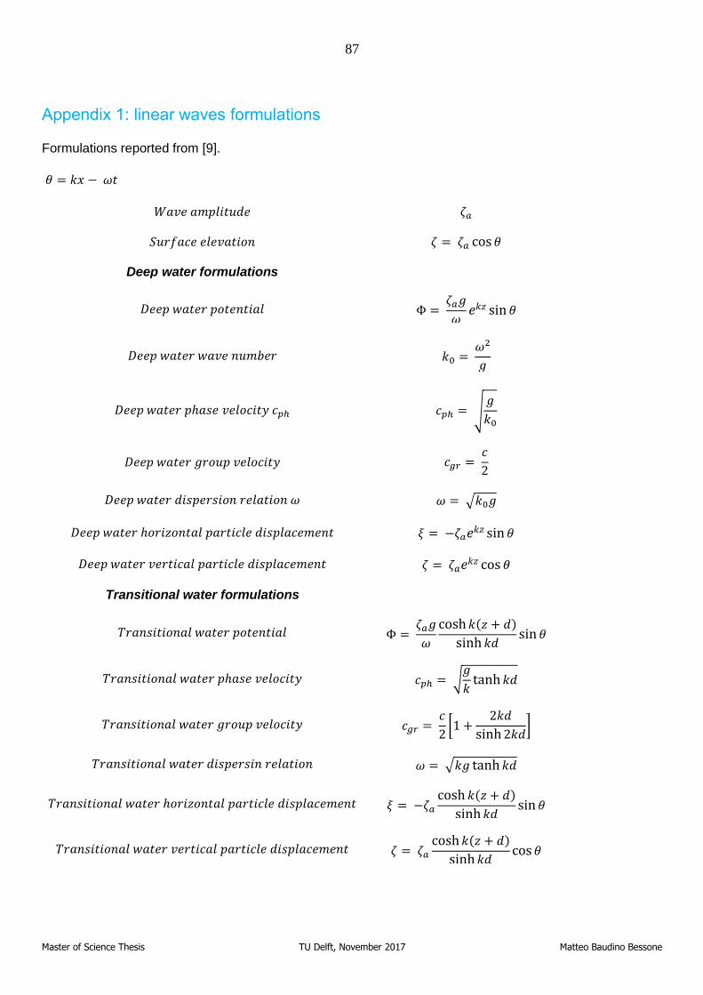
87


Appendix 1: linear waves formulations

Formulations reported from [9].

𝜃 = 𝑘𝑥 − 𝜔𝑡

𝑊𝑎𝑣𝑒 𝑎𝑚𝑝𝑙𝑖𝑡𝑢𝑑𝑒 𝜁𝑎

𝑆𝑢𝑟𝑓𝑎𝑐𝑒 𝑒𝑙𝑒𝑣𝑎𝑡𝑖𝑜𝑛 𝜁 = 𝜁𝑎 cos𝜃

Deep water formulations

𝐷𝑒𝑒𝑝 𝑤𝑎𝑡𝑒𝑟 𝑝𝑜𝑡𝑒𝑛𝑡𝑖𝑎𝑙 Φ = 𝜁𝑎𝑔

𝜔𝑒𝑘𝑧 sin 𝜃

𝐷𝑒𝑒𝑝 𝑤𝑎𝑡𝑒𝑟 𝑤𝑎𝑣𝑒 𝑛𝑢𝑚𝑏𝑒𝑟 𝑘0 = 𝜔2

𝑔

𝐷𝑒𝑒𝑝 𝑤𝑎𝑡𝑒𝑟 𝑝ℎ𝑎𝑠𝑒 𝑣𝑒𝑙𝑜𝑐𝑖𝑡𝑦 𝑐𝑝ℎ 𝑐𝑝ℎ = √𝑔

𝑘0

𝐷𝑒𝑒𝑝 𝑤𝑎𝑡𝑒𝑟 𝑔𝑟𝑜𝑢𝑝 𝑣𝑒𝑙𝑜𝑐𝑖𝑡𝑦 𝑐𝑔𝑟 = 𝑐

2

𝐷𝑒𝑒𝑝 𝑤𝑎𝑡𝑒𝑟 𝑑𝑖𝑠𝑝𝑒𝑟𝑠𝑖𝑜𝑛 𝑟𝑒𝑙𝑎𝑡𝑖𝑜𝑛 𝜔 𝜔 = √𝑘0𝑔

𝐷𝑒𝑒𝑝 𝑤𝑎𝑡𝑒𝑟 ℎ𝑜𝑟𝑖𝑧𝑜𝑛𝑡𝑎𝑙 𝑝𝑎𝑟𝑡𝑖𝑐𝑙𝑒 𝑑𝑖𝑠𝑝𝑙𝑎𝑐𝑒𝑚𝑒𝑛𝑡 𝜉 = −𝜁𝑎𝑒𝑘𝑧 sin 𝜃

𝐷𝑒𝑒𝑝 𝑤𝑎𝑡𝑒𝑟 𝑣𝑒𝑟𝑡𝑖𝑐𝑎𝑙 𝑝𝑎𝑟𝑡𝑖𝑐𝑙𝑒 𝑑𝑖𝑠𝑝𝑙𝑎𝑐𝑒𝑚𝑒𝑛𝑡 𝜁 = 𝜁𝑎𝑒𝑘𝑧 cos 𝜃

Transitional water formulations

𝑇𝑟𝑎𝑛𝑠𝑖𝑡𝑖𝑜𝑛𝑎𝑙 𝑤𝑎𝑡𝑒𝑟 𝑝𝑜𝑡𝑒𝑛𝑡𝑖𝑎𝑙 Φ = 𝜁𝑎𝑔

𝜔

cosh𝑘(𝑧 + 𝑑)

sinh𝑘𝑑sin𝜃

𝑇𝑟𝑎𝑛𝑠𝑖𝑡𝑖𝑜𝑛𝑎𝑙 𝑤𝑎𝑡𝑒𝑟 𝑝ℎ𝑎𝑠𝑒 𝑣𝑒𝑙𝑜𝑐𝑖𝑡𝑦 𝑐𝑝ℎ = √𝑔

𝑘tanh𝑘𝑑

𝑇𝑟𝑎𝑛𝑠𝑖𝑡𝑖𝑜𝑛𝑎𝑙 𝑤𝑎𝑡𝑒𝑟 𝑔𝑟𝑜𝑢𝑝 𝑣𝑒𝑙𝑜𝑐𝑖𝑡𝑦 𝑐𝑔𝑟 = 𝑐

2[1 +

2𝑘𝑑

sinh2𝑘𝑑]

𝑇𝑟𝑎𝑛𝑠𝑖𝑡𝑖𝑜𝑛𝑎𝑙 𝑤𝑎𝑡𝑒𝑟 𝑑𝑖𝑠𝑝𝑒𝑟𝑠𝑖𝑛 𝑟𝑒𝑙𝑎𝑡𝑖𝑜𝑛 𝜔 = √𝑘𝑔 tanh𝑘𝑑

𝑇𝑟𝑎𝑛𝑠𝑖𝑡𝑖𝑜𝑛𝑎𝑙 𝑤𝑎𝑡𝑒𝑟 ℎ𝑜𝑟𝑖𝑧𝑜𝑛𝑡𝑎𝑙 𝑝𝑎𝑟𝑡𝑖𝑐𝑙𝑒 𝑑𝑖𝑠𝑝𝑙𝑎𝑐𝑒𝑚𝑒𝑛𝑡 𝜉 = −𝜁𝑎cosh 𝑘(𝑧 + 𝑑)

sinh𝑘𝑑sin𝜃

𝑇𝑟𝑎𝑛𝑠𝑖𝑡𝑖𝑜𝑛𝑎𝑙 𝑤𝑎𝑡𝑒𝑟 𝑣𝑒𝑟𝑡𝑖𝑐𝑎𝑙 𝑝𝑎𝑟𝑡𝑖𝑐𝑙𝑒 𝑑𝑖𝑠𝑝𝑙𝑎𝑐𝑒𝑚𝑒𝑛𝑡 𝜁 = 𝜁𝑎cosh𝑘(𝑧 + 𝑑)

sinh𝑘𝑑cos𝜃

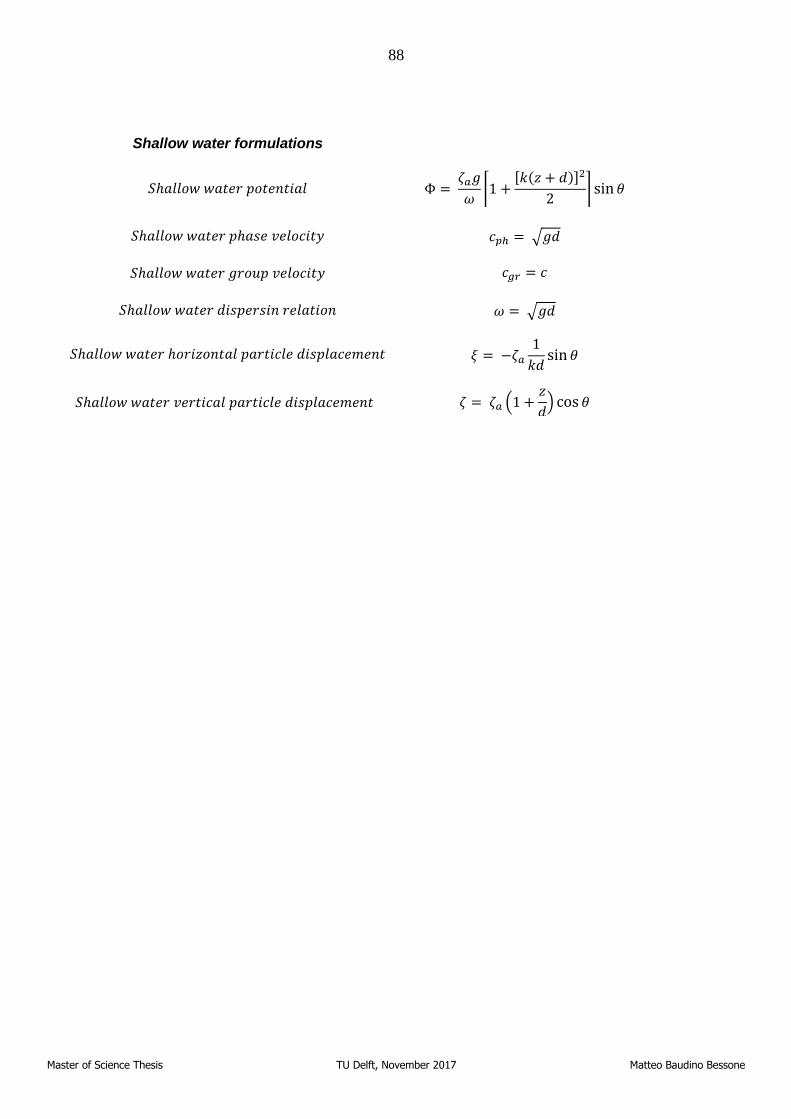
88


Shallow water formulations

𝑆ℎ𝑎𝑙𝑙𝑜𝑤 𝑤𝑎𝑡𝑒𝑟 𝑝𝑜𝑡𝑒𝑛𝑡𝑖𝑎𝑙 Φ = 𝜁𝑎𝑔

𝜔[1 +

[𝑘(𝑧 + 𝑑)]2

2] sin𝜃

𝑆ℎ𝑎𝑙𝑙𝑜𝑤 𝑤𝑎𝑡𝑒𝑟 𝑝ℎ𝑎𝑠𝑒 𝑣𝑒𝑙𝑜𝑐𝑖𝑡𝑦 𝑐𝑝ℎ = √𝑔𝑑

𝑆ℎ𝑎𝑙𝑙𝑜𝑤 𝑤𝑎𝑡𝑒𝑟 𝑔𝑟𝑜𝑢𝑝 𝑣𝑒𝑙𝑜𝑐𝑖𝑡𝑦 𝑐𝑔𝑟 = 𝑐

𝑆ℎ𝑎𝑙𝑙𝑜𝑤 𝑤𝑎𝑡𝑒𝑟 𝑑𝑖𝑠𝑝𝑒𝑟𝑠𝑖𝑛 𝑟𝑒𝑙𝑎𝑡𝑖𝑜𝑛 𝜔 = √𝑔𝑑

𝑆ℎ𝑎𝑙𝑙𝑜𝑤 𝑤𝑎𝑡𝑒𝑟 ℎ𝑜𝑟𝑖𝑧𝑜𝑛𝑡𝑎𝑙 𝑝𝑎𝑟𝑡𝑖𝑐𝑙𝑒 𝑑𝑖𝑠𝑝𝑙𝑎𝑐𝑒𝑚𝑒𝑛𝑡 𝜉 = −𝜁𝑎1

𝑘𝑑sin 𝜃

𝑆ℎ𝑎𝑙𝑙𝑜𝑤 𝑤𝑎𝑡𝑒𝑟 𝑣𝑒𝑟𝑡𝑖𝑐𝑎𝑙 𝑝𝑎𝑟𝑡𝑖𝑐𝑙𝑒 𝑑𝑖𝑠𝑝𝑙𝑎𝑐𝑒𝑚𝑒𝑛𝑡 𝜁 = 𝜁𝑎 (1 +𝑧

𝑑) cos 𝜃

89


Appendix 2: discrete momentum equations

This section follows the derivation of CG discretisation of the Navier-Stokes equation described in [33]. For reasons of conciseness, the rigorous notation of differential equation is dropped in this appendix. The three-dimensional domain Ω direction will be indicated as 𝑖, 𝑗 = 1,2,3. The ith component of velocity can be indicated

as 𝑢𝑖. The derivative with respect to space will be indicated as ,𝑖 and respect to time as ,𝑡.

Equations 3.1.1.1 and 3.1.1.2 can be greatly simplified assuming an incompressible fluid, and considering a Newtonian fluid, which is stating that [53]

𝜌 = 𝑐𝑜𝑛𝑠𝑡,

𝑆̿ = 2𝜇𝜖�̇�𝑗 = 2𝜇 (

𝑣𝑖,𝑗 + 𝑣𝑖,𝑗

2),

where 𝜌 is the density, 𝑆̿ is the deviatoric part of the stress tensor, 𝜇 is the dynamic viscosity and 𝜖�̇�𝑗 is the

strain rate. Under these assumptions, the incompressible continuity equation 3.1.1.1 and the momentum equation 3.1.1.2 become

𝑣𝑖,𝑖 = 0.

Which is equal to say that the velocity is divergence-free

𝜌𝑣𝑖,𝑡 + 𝜌(𝑣𝑖𝑣𝑗),𝑗− 𝜇𝑣𝑖,𝑗𝑗 = −𝑝,𝑖 + 𝑓,𝑖.

This set of equations is fulfilled by a set of properly arranged boundary conditions:

𝑣𝑖 = 𝑑𝑖(𝑥𝑗, 𝑡) 𝑜𝑛 𝜕Ω𝑔𝑖

𝑝 = �̂�(𝑥𝑗, 𝑡) 𝑜𝑛 𝜕Ωℎ

is equivalent to imposing a velocity on a boundary 𝜕Ω𝑔𝑖, so-called Dirichlet boundary condition.

𝜇𝑣𝑖,𝑗𝑛𝑗 = ℎ𝑖(𝑥𝑘 , 𝑡) 𝑜𝑛 𝜕Ωℎ

is equivalent to impose a stress on the boundary 𝜕Ωℎ, so-called Neumann boundary condition.

90


𝑢𝑖(𝑥𝑗, 0) = 𝑢01(𝑥𝑗) 𝑜𝑛 Ω ,

𝑝(𝑥𝑗, 0) = 𝑝01(𝑥𝑗) 𝑜𝑛 Ω ,

which is equivalent to state the initial condition in the whole domain at t=0.

The weak formulation of the momentum equation is obtained following the four steps prescribed in 3.1.2, multiplication per the test function 𝑤𝑖, integration over the physical domain and integration by part of the advective and viscous terms, to lower the continuity required for the solution and to introduce the boundary conditions. The weak form results to be:

∫𝑤𝑖𝜌

Ω

𝑢𝑖,𝑡𝑑Ω −∫𝑤𝑖,𝑗𝜌

Ω

𝑢𝑖𝑢𝑗𝑑Ω +∫ 𝑤𝑖𝜌

Ωℎ

𝑢𝑖𝑢𝑗𝑛𝑖𝑑Ωℎ +∫𝑤𝑖,𝑗𝜇

Ω

𝑢𝑖,𝑗𝑑Ω

= −∫𝑤𝑖𝑝,𝑖

Ω

𝑑Ω +∫𝑤𝑖𝑓𝑖

Ω

𝑑Ω+∫ 𝑤𝑖ℎ𝑖

Ωℎ

𝑑Ωℎ.

Introducing the discrete trial and test functions according to 3.1.2.1 and 3.1.2.2:

∫ 𝜓𝐼𝜌𝜙𝐽𝑢𝑖,𝑡𝐽dΩ−

Ω

∫ 𝜓,𝑗𝐼𝜌𝑢𝑗𝜙𝐽𝑢𝑖𝐽

Ω

𝑑Ω +∫ 𝜓𝐼𝜌

Ωℎ

𝑢𝑗𝑛𝑗𝜙𝐽𝑢𝑖𝐽𝑑Ωℎ +∫ 𝜓,𝑗𝐼𝜇𝜙𝐽𝑢𝑖𝐽

Ω

𝑑Ω

= −∫𝜓𝐼𝑝,𝑖

Ω

𝑑Ω +∫𝜓𝐼𝑓𝑖

Ω

𝑑Ω+∫ 𝜓𝐼ℎ𝑖

Ωℎ

𝑑Ωℎ.

Where 𝐼 , 𝐽 refer to the Ith and Jth node of the mesh.

Now the following matrixes can be introduced:

∫𝜓𝐼𝜌𝜙𝐽dΩ = [𝑀𝑚]𝐼𝐽

Ω

,

−∫ 𝜓𝐼,𝑗𝜌𝑢𝑗𝐽𝜙𝑑Ω

Ω

+∫ 𝜓𝐼𝜌

Ωℎ

𝑢𝑗𝐽𝑛𝑗𝜙𝐽𝑑 = [𝑁𝑚]𝐼𝐽,

∫ 𝜓,𝑗𝐼𝜇𝜙𝐽𝑢𝑖𝐽

Ω

𝑑Ω = [K𝑚]𝐼𝐽,

91


−∫𝜓𝐼𝑝,𝑖

Ω

𝑑Ω = [p𝑚]𝐼 ,

∫𝜓𝐼𝑓𝑖

Ω

𝑑Ω = [f𝑚]𝐼 ,

∫ 𝜓𝐼ℎ𝑖

Ωℎ

𝑑Ωℎ = [𝑏𝑚]𝐼,

with 𝑀𝑚 the mass matrix, 𝑁𝑚 the advection matrix, K𝑚 the diffusion matrix, p𝑚 the pressure gradient matrix,

f𝑚 body force matrix and 𝑏𝑚 the discretised natural boundary conditions matrix. The resultant equation is

[𝑀𝑚]𝐼𝐽𝑢𝑖,𝑡𝐽 + [𝑁𝑚]𝐼𝐽𝑢𝑖𝐽 + [K𝑚]𝐼𝐽𝑢𝑖𝐽 = [p𝑚]𝐼 + [f𝑚]𝐼 + [𝑏𝑚]𝐼.

92


Bibliography

[1] Global Wind Energy Council, “Global wind 2016 report,” 2016. [Online]. Available:

http://gwec.net/global-figures/global-offshore/. [Accessed 24 10 2017].

[2] M. D. Esteban, J. J. Diez, J. S. Lòpez and V. Negro, “Why offshore wind energy?,” Renewable Energy,

vol. 36, pp. 444-450, 2010.

[3] J. Cruz and M. Atcheson, Floating Offshore Wind Energy, Lisbon, Portugal: Springer International

Publishing, 2016.

[4] S. Butterfield, W. Musial, J. Jonkman and P. Sclavounos, “Engineering Challenges for Floating

Offshore Wind Turbines,” in 2005 Copenhagen Offshore Wind Conference , Copenhagen, October 26-

28, 2005.

[5] W. Finnegan, M. Meere and J. Goggins, “The wave excitation forces on a truncated vertical cylinder,”

Journal of Fluids and Structures, vol. 40, pp. 201-213, 2013.

[6] A. Viré, J. Spinneken, M. D. Piggot, C. C. Pain and S. C. Kramer, “Application of the immersed-body

method to simulate wave-structure interactions,” European Journal of Mechanics B/Fluids, Vols. 55,

Part 2, pp. 330 - 339, 10 November 2015.

[7] Aquaret, “Aquaret, Delivering Knowledge and Understanding,” 2012. [Online]. Available:

http://www.aquaret.com/. [Accessed 2017 10 24].

[8] National Renewable Energy Laboratory, “Offshore Design Tools and Methods,” [Online]. Available:

https://www.nrel.gov/wind/offshore-tools-methods.html. [Accessed 24 10 2017].

[9] W. Finnegan and J. Goggins, “Numerical simulation of linear water waves and wave–structure

interaction,” Ocean Engineering, vol. 43, pp. 23-31, 2012.

[10] A. Viré, J. Xiang, F. Milthalter, P. E. Farrell, M. D. Piggott, J. P. Latham, D. Pavlidis and C. C. Pain,

“Modelling of fluid–solid interactions using an adaptive mesh fluid model coupled with a combined

finite–discrete element model,” Ocean Dynamics, vol. 62, pp. 1487-1501, 2012.

[11] K. J. Bai, “The added mass of two-dimensional cylinders heaving in water of finite depth,” Journal of

Fluid Mechanics, vol. 81, no. 1, pp. 85-105, 1976.

[12] J.-F. Lee, “On the heave radiation of a rectangular structure,” Ocean Engineering, vol. 22, pp. 19-34,

1995.

[13] Y. H. Zheng, Y. G. You and Y. M. Shen, “On the radiation and diffraction of water waves by a

rectangular buoy,” Ocean Engineering, vol. 31, pp. 1063-1082, 2004.

[14] P. Troch, “A Review of Numerical Modelling of Wave Energy Converter Arrays,” in OMAE

conference, Rio de Janeiro, Brsil, 2012.

[15] A. R. Henderson and D. Witcher, “Floating Offshore Wind Energy - A Review of the Current Status

and an Assessment of the Prospects,” Wind Engineering, vol. 34, pp. 01-16, 2010.

[16] EWEA, European Wind Energy Association, “Deep water. The next step for offshore wind energy,”

European Wind Energy Association, July 2013.

[17] C. M. Wang, T. Utsunomiya, S. C. Wee and Y. S. Choo, “Research on floating wind turbines: a

literature survey,” The IES Journal Part A: Civil & Structural Engineering, vol. 3:4, pp. 267-277, 20

October 2010.

[18] L. O. Garza-Rios, M. M. Bernistas, K. Nishimoto and J. P. J. Matsuura, “Dynamics of Spread Mooring

Systems With Hybrid Mooring Lines,” Journal of Offshore Mechanics and Arctic Engineering, vol.

122, pp. 274-281, 19 July 2000.

[19] M. Borg, A. Shires and M. Collu, “Offshore floating vertical axis wind turbines, dynamics modelling

state,” Renewable and Sustainable Energy Reviews, vol. 39, no. 2014.07.096, pp. 1214-1225,

November 2015.

93


[20] M. Borg and M. Collu, “A comparison between the dynamics of horizontal and vertical axis offshore

floating wind turbines,” Philosophical Transactions of the Royal Society A: Mathematical, Physical &

Engineering Sciences, vol. 373, no. 20140076, 12 January 2015.

[21] G. Clauss, E. Lehmann and C. Östergaard, Offshore structures volume I, London: Springer-Verlag, 25

september 2014.

[22] J. N. Newman, Marine Hydrodynamics, Cambridge, Massachusetts and London, England: The MIT

Press, 1977.

[23] T. Sarpkaya, Wave forces on offshore structures, Cambridge, UK: Cambridge University Press, 2010.

[24] G. B. Airy, “Tides and waves,” Encyclopedia Metropopolitana, 1845, pp. 192: 241-396.

[25] O. S. Madsen, “Waves generated by a piston-type wavemaker,” in 12th International Conference on

Coastal Engineering, Washington, D.C, United States, 1970.

[26] J. M. J. Journée and W. W. Massie, Offshore hydromechanics, Delft: Delft University of Technology,

January 2001.

[27] B. M. Sumer and J. Fredsøe, Hydrodynamics around cylindrical structures, Singapore: World

Scientific, 2006.

[28] T. Than Toan, K. Dong-Hyun and N. Ba Hieu, “Aerodynamic Interference Effect of Huge Wind

Turbine Blades With Periodic Surge Motions Using Overset Grid-Based Computational Fluid

Dynamics Approach,” Journal of Solar Energy Engineering, vol. 137, 2015.

[29] W. Koo and J.-D. Kim, “Simplified formulas of heave added mass coefficients at high frequency for

various two-dimensional bodies in a finite water depth,” International Journal of Naval Architecture

and Ocean Engineering, vol. 7, no. 1, p. 115–127, 2015.

[30] R. C. MacCamy and R. A. Fuchs, “Wave forces on piles: A diffraction theory,” Technical

memorandum, Beach Erosion Board, 1954.

[31] J. H. Vugts, “The hydrodynamic coefficients for swaying, heaving and rolling cylinders on a free

surface,” Shipbuilding Laboratory, Technical University Delft, 1968.

[32] Imperial College London, “fluidityproject,” [Online]. Available: http://fluidityproject.github.io/.

[Accessed 11 10 2017].

[33] C. Wilson, “Modelling multiple-material flows on adaptive unstructured meshes,” Department of Earth

Science and Engineering, Imperial College London, 2009.

[34] Department of Earth Science and Engineering, Imperial College London, “fluidity manual, version

4.1,” London, 2015.

[35] O. C. Zienkiewicz, R. L. Taylor and J. Z. Zhu, The Finite Element Method: Its Basis and

Fundamentals, Elsevier Ltd, 2013.

[36] C. J. Cotter, D. A. Ham and C. C. Pain, “A mixed discontinuous/continuous finite element pair for

shallow-water,” Ocean Modelling, vol. 26, pp. 86-90, 2008.

[37] J. Spinneken, V. Heller, S. Kramer, M. Piggott and A. Viré, “Assessment of an Advanced Finite

Element Tool for the Simulation of Fully-nonlinear Gravity Water Waves,” in International Offshore

and Polar Engineering Conference, Rhodes, Greece, 2012.

[38] A. Viré, J. Xiang and C. C. Pain, “An immersed-shell method for modelling fluid–structure

interactions,” Philosophical transaction Royal Society publishing A, vol. 373, no. 20140085., 2015.

[39] P. Yang, J. Xiang, F. Fang, D. Pavlidis, J. P. Latham and C. C. Pain, “Modelling of fluid–structure

interaction with multiphase viscous flows using an immersed-body method,” Journal of Computational

Physics, vol. 321, p. 571–592, 2015.

[40] P. E. Farrell and J. R. Maddison, “Conservative interpolation between volume meshes by local

Galerkin projection,” Computer Methods in Applied Mechanics and Engineering, vol. 200, pp. 89-100,

2010.

94


[41] J. A. Cottrell, T. J. R. Hughes and Y. Bazilevs, Isogeometric Analysis, Towards Integration of CAD

and FEA, Chirchester, UK: John Wiley and Sons, 2009.

[42] R. H. Bartels, J. C. Beatty and B. A. Barsky, An Introduction to Splines for use in Computer Graphics

and Geometrical Modeling, Los Altos, USA: Morgan Kaufmann Publishers , 1987.

[43] L. Piegl and W. Tiller, The NURBS Book, Berlin: Springer-Verlag, 1997.

[44] J. Peterson, “How to use Knot Vectors,” June 1990. [Online]. Available:

http://www.saccade.com/writing/graphics/KnotVectors.pdf. [Accessed 28 1 2017].

[45] K. J. Williams, “An experimental study of wave-obstacle interaction in a two-dimensional domain,”

Journal of Hydarulic Research, vol. 26, no. 4, pp. 463-482, 2010.

[46] K. Hayata, M. Koshiba and M. Suzuki, “A Method for Improving the Accuracy of Finite-Element

Solutions Using the Extrapolation Method,” Electronics and Communications in Japan, vol. 69, pp.

115-121, 1986.

[47] L. Chen and J. Zhou, “Analyses of wave forces on surface piercing vertical cylinders of intermediate

scale,” Procedia Engineering, vol. 126, pp. 290-294, 2015.

[48] B. T. Paulsen, H. Bredmose, H. B. Bingham and N. G. Jacobsen, “Forcing of a bottom-mounted

circular cylinder,” Journal of Fluid Mechanics, vol. 755, pp. 1-34, 2014.

[49] H. Babaei, S. Baker and A. Cornett, “Validation of a CFD tool for studying the interaction of extreme

waves with offshore gravity-based structures,” in Proceedings of the 6th International Conference on

the Application of Physical Modelling in Coastal and Port Engineering and Science (Coastlab16),

Ottawa, Canada, 2016.

[50] Q. Ma, Advances in Numerical Simulation of Nonlinear Water Waves, Singapore: World Scientific,

2010.

[51] L. Bonfiglio, S. Brizzolara and C. Chrissostomidis, “Added Mass and Damping of Oscillating Bodies:

a fully viscous numerical approach,” in Recent Advances in Fluid Mechanics, Heat & Mass Transfer

and Biology.

[52] N. Drimer, Y. Agnon and M. Stiassnie, “A simplified analytical model for a floating breakwater in

water of finite depth,” Applied Ocean Research, vol. 14, pp. 33-41, 1992.

[53] A. Segal, fem notes from Finite element methods for the incompressible Navier-Stokes equations, Delft

University of Technology, 2017.

[54] the japan times, “japantimes.co.jp,” 11 11 2013. [Online]. Available:

http://www.japantimes.co.jp/news/2013/11/11/national/floating-wind-farm-debuts-off-

fukushima/#.WRCmqtLyhpg. [Accessed 08 05 2017].

[55] “offshorewind.biz,” 25 11 2016. [Online]. Available:

http://www.offshorewind.biz/2016/11/25/seatwirl-raising-funds-to-develop-full-scale-vawt-floating-

turbine-video/. [Accessed 08 05 2017].

Documents

Master of Science Thesis TU Delft, November 2017 Matteo