Embed Size (px)
Citation preview
MASTER
CONTROLLER
- USER MANUAL (Ver. 1.5) -
January 2016
2
Content
Introduction ..................................................................................................................................... 4
1.1 Master Controller .................................................................................................................... 4
1.2 Operating modes and network architectures ......................................................................... 5
1.2.1 Standalone mode ............................................................................................................ 5
1.2.2 Integrated mode .............................................................................................................. 6
1.3 Hardware specifications .......................................................................................................... 7
MC setup ......................................................................................................................................... 9
2.1 Required hardware parts ........................................................................................................ 9
2.2 Configuring the slave controllers ............................................................................................ 9
2.2.1 Installation of the system macros file ............................................................................. 9
2.2.2 Software setup .............................................................................................................. 10
2.2.3 Hardware setup ............................................................................................................. 10
2.3 Configuring MC ...................................................................................................................... 11
2.3.1 Powering up ................................................................................................................... 11
2.3.2 Accessing the MC operating system .............................................................................. 11
Navigating through the MC operating system .............................................................................. 15
3.1 Configuring the MC firmware ................................................................................................ 15
3.2 MC program editor ................................................................................................................ 16
3.3 Running an MC program ....................................................................................................... 18
3.4 Terminating a running MC program ...................................................................................... 21
Tutorial .......................................................................................................................................... 22
4.1 Program flowchart ................................................................................................................. 22
4.2 Standalone mode execution.................................................................................................. 24
4.2.1 Program ......................................................................................................................... 24
4.3 Integrated (Ethernet/IP) mode execution ............................................................................. 25
4.3.1 Program ......................................................................................................................... 25
4.3.2 EDS file installation for Allen-Bradley PLCs ................................................................... 26
4.3.3 Setting up the communication between Studio 5000 / RSLogix 5000 and MC ............ 27
4.3.4 PLC program example.................................................................................................... 33
4.3.5 Importing application-specific controller tags .............................................................. 34
Program structure ............................................................................................................................. 36
Programming syntax.......................................................................................................................... 36
Function list ....................................................................................................................................... 37

January 2016
3
IO register – the bridge between MC and standard industrial protocols ......................................... 44
IO register mapping for Ethernet/IP .............................................................................................. 44
IO register mapping for PROFINET ................................................................................................ 45
Variable list ........................................................................................................................................ 46

January 2016
4
Introduction
1.1 Master Controller
The Master Controller (MC) shown in Figure 1 is a device that coordinates multiple SMAC CANopen-
based slave controllers in a multi-axis motion system, and at the same time can communicate with a
PLC through standard industrial ethernet protocols such as Ethernet/IP and PROFINET. The hardware
platform of MC is a mini computer running on a Linux operating system. Additionally, there is a
daughter board that provides interfaces to a CANopen network and a 24 VDC power supply.
The control and communication functionalities of MC are accommodated by a firmware that runs
within the MC operating system. To create an MC program, a set of commands and parameters (having
a syntax similar to the SMAC LCC control center program) is written in a configuration software that
can be accessed from the MC operating system.
Further information about the MC features, specifications, operating instructions and tutorials are
presented in the following sections of this manual.
Figure 1. Master controller.
January 2016
5
1.2 Operating modes and network architectures
Depending on the context of MC application in a given industrial/laboratory setting, there are two MC
operating modes that are firmware-dependent, as follow
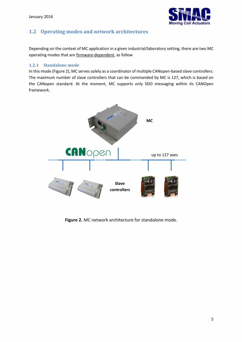
1.2.1 Standalone mode
In this mode (Figure 2), MC serves solely as a coordinator of multiple CANopen-based slave controllers.
The maximum number of slave controllers that can be commanded by MC is 127, which is based on
the CANopen standard. At the moment, MC supports only SDO messaging within its CANOpen
framework.
Figure 2. MC network architecture for standalone mode.
up to 127 axes
MC
Slave
controllers
January 2016
6
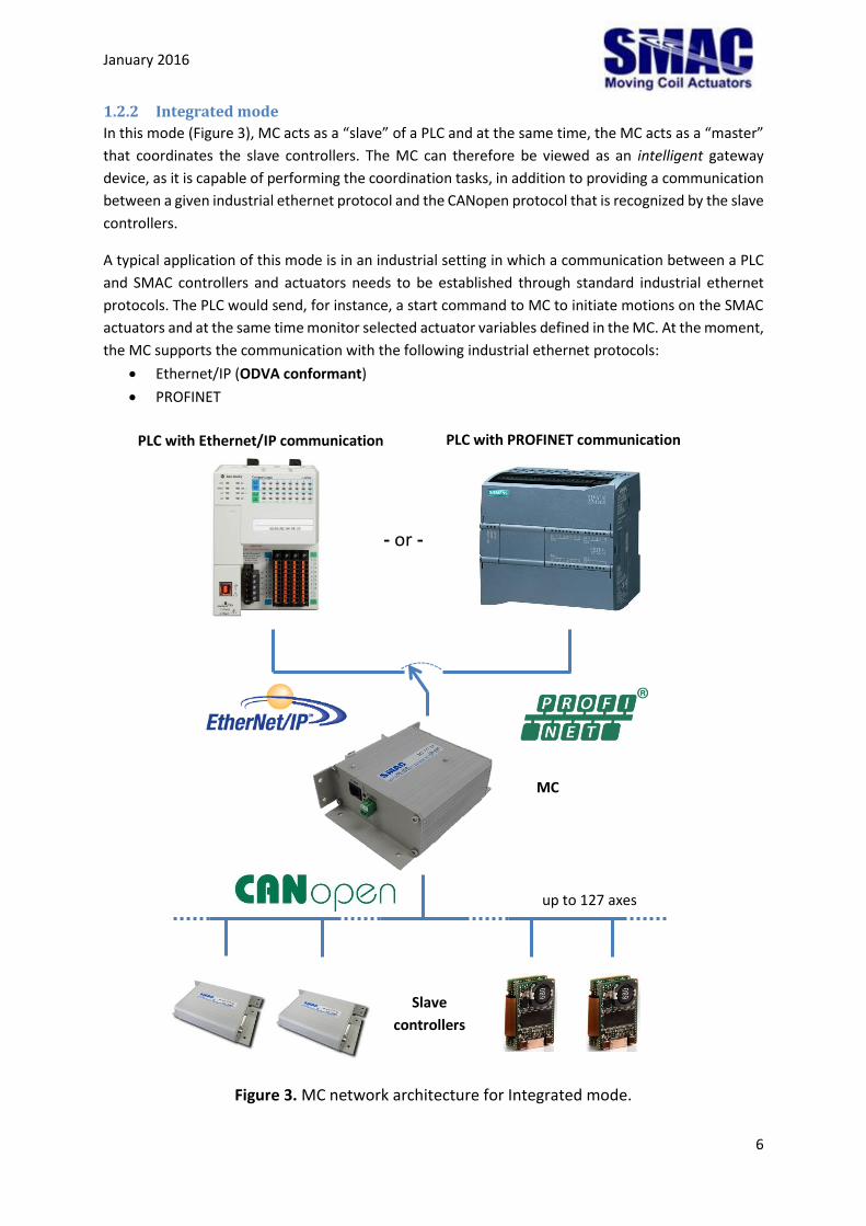
1.2.2 Integrated mode
In this mode (Figure 3), MC acts as a “slave” of a PLC and at the same time, the MC acts as a “master”
that coordinates the slave controllers. The MC can therefore be viewed as an intelligent gateway
device, as it is capable of performing the coordination tasks, in addition to providing a communication
between a given industrial ethernet protocol and the CANopen protocol that is recognized by the slave
controllers.
A typical application of this mode is in an industrial setting in which a communication between a PLC
and SMAC controllers and actuators needs to be established through standard industrial ethernet
protocols. The PLC would send, for instance, a start command to MC to initiate motions on the SMAC
actuators and at the same time monitor selected actuator variables defined in the MC. At the moment,
the MC supports the communication with the following industrial ethernet protocols:
Ethernet/IP (ODVA conformant)
PROFINET
Figure 3. MC network architecture for Integrated mode.
PLC with PROFINET communication PLC with Ethernet/IP communication
up to 127 axes
MC
Slave
controllers
- or -
January 2016
7
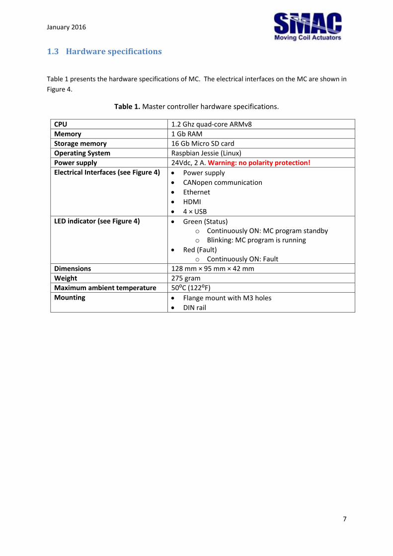
1.3 Hardware specifications
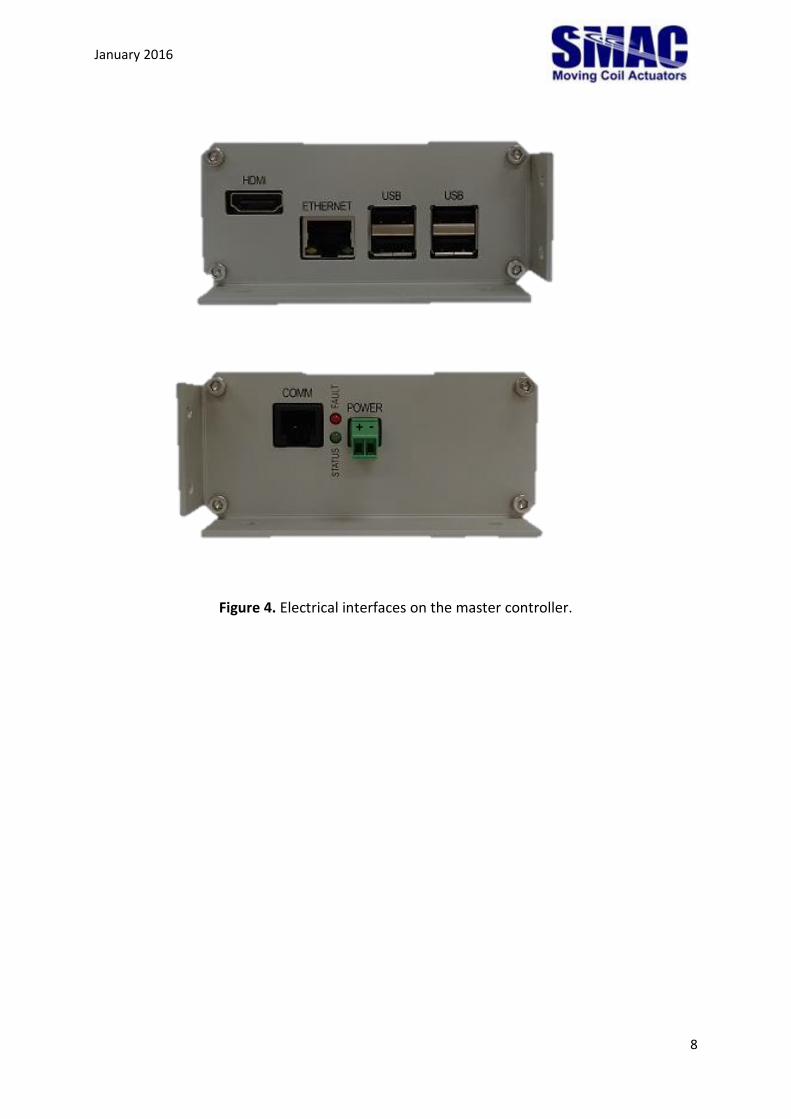
Table 1 presents the hardware specifications of MC. The electrical interfaces on the MC are shown in
Figure 4.
Table 1. Master controller hardware specifications.
CPU 1.2 Ghz quad-core ARMv8
Memory 1 Gb RAM
Storage memory 16 Gb Micro SD card
Operating System Raspbian Jessie (Linux)
Power supply 24Vdc, 2 A. Warning: no polarity protection!
Electrical Interfaces (see Figure 4) Power supply
CANopen communication
Ethernet
HDMI
4 × USB LED indicator (see Figure 4) Green (Status)
o Continuously ON: MC program standby o Blinking: MC program is running
Red (Fault) o Continuously ON: Fault
Dimensions 128 mm × 95 mm × 42 mm
Weight 275 gram
Maximum ambient temperature 50⁰C (122⁰F)
Mounting Flange mount with M3 holes
DIN rail
January 2016
8
Figure 4. Electrical interfaces on the master controller.
+ -
January 2016
9
MC setup
2.1 Required hardware parts
The following is the list of required hardware parts to setup the MC to form a multi-axis motion system:
Master controller
24 VDC, 2 A power supply
120 ohm terminating resistor for the CANopen network
Ethernet LAN cable
PC with a SMAC LCC Control Center software installed, for the following purposes:
o Access the MC operating system
o Perform settings on the slave controllers
SMAC controllers and actuators for the intended application. Note that only the following
controllers can be used:
o LCC (loaded with a firmware version 3.0R or higher)
o CBC
HDMI cable (optional)
HDMI compatible monitor (optional)
USB mouse (optional)
USB keyboard (optional)
2.2 Configuring the slave controllers
2.2.1 Installation of the system macros file
To be operated by MC, system macros need to be downloaded to the slave controllers. This can be
done through the LCC Control Center program, provided a file containing the system macros is installed.
The installation procedure is as follow:
1. Obtain the file “System macros V2.mlm” provided with this manual. In case it is not available,
contact [email protected]
2. Copy the file, and paste (overwrite) it in the LCC Control Center installation folder typically
located in: C:\..\SMAC\LCC Control Center
After the above procedure, the system macros will be automatically downloaded to the slave
controllers every time the button “save all in controller” (in the LCC Control Center program) is clicked.
As a consequence of the previous system macros, the following features (which are normally available)
are reserved for the MC and therefore cannot be used in programming the slave macros:
Macros 55 – 59
General purpose registers W95 – W100
January 2016
10
2.2.2 Software setup
The software setup procedure for the slave controllers is as follow:
1. Download the required actuator configuration file to each slave controller.
2. Assign different node IDs to all the slave controllers that will be connected to MC. Note down
the node IDs, as these will be used in writing an MC program.
3. If required, macros can be programmed in the slave controller, which can be called by MC.
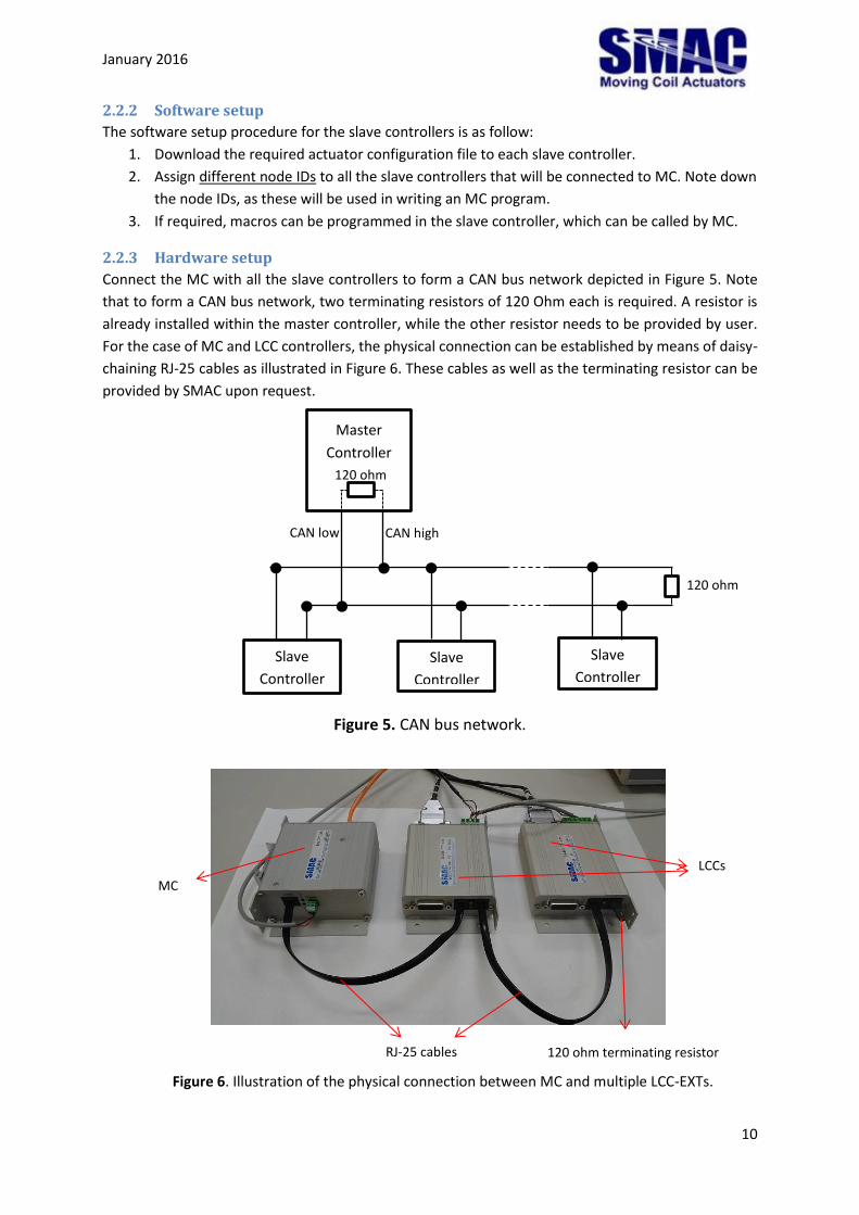
2.2.3 Hardware setup
Connect the MC with all the slave controllers to form a CAN bus network depicted in Figure 5. Note
that to form a CAN bus network, two terminating resistors of 120 Ohm each is required. A resistor is
already installed within the master controller, while the other resistor needs to be provided by user.
For the case of MC and LCC controllers, the physical connection can be established by means of daisy-
chaining RJ-25 cables as illustrated in Figure 6. These cables as well as the terminating resistor can be
provided by SMAC upon request.
Figure 5. CAN bus network.
Figure 6. Illustration of the physical connection between MC and multiple LCC-EXTs.
Master
Controller
120 ohm
CAN low CAN high
120 ohm
Slave
Controller
Slave
Controller
Slave
Controller
LCCs
MC
RJ-25 cables
120 ohm terminating resistor
January 2016
11
2.3 Configuring MC
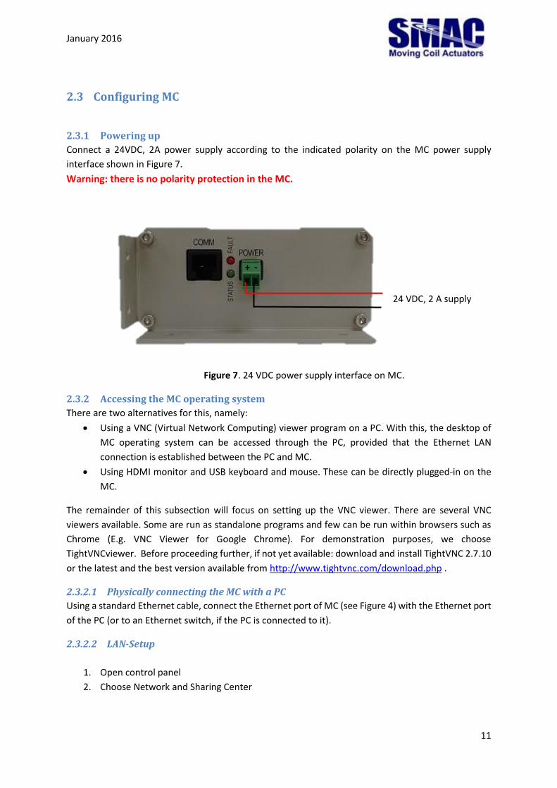
2.3.1 Powering up
Connect a 24VDC, 2A power supply according to the indicated polarity on the MC power supply
interface shown in Figure 7.
Warning: there is no polarity protection in the MC.
Figure 7. 24 VDC power supply interface on MC.
2.3.2 Accessing the MC operating system
There are two alternatives for this, namely:
Using a VNC (Virtual Network Computing) viewer program on a PC. With this, the desktop of
MC operating system can be accessed through the PC, provided that the Ethernet LAN
connection is established between the PC and MC.
Using HDMI monitor and USB keyboard and mouse. These can be directly plugged-in on the
MC.
The remainder of this subsection will focus on setting up the VNC viewer. There are several VNC
viewers available. Some are run as standalone programs and few can be run within browsers such as
Chrome (E.g. VNC Viewer for Google Chrome). For demonstration purposes, we choose
TightVNCviewer. Before proceeding further, if not yet available: download and install TightVNC 2.7.10
or the latest and the best version available from http://www.tightvnc.com/download.php .
2.3.2.1 Physically connecting the MC with a PC
Using a standard Ethernet cable, connect the Ethernet port of MC (see Figure 4) with the Ethernet port
of the PC (or to an Ethernet switch, if the PC is connected to it).
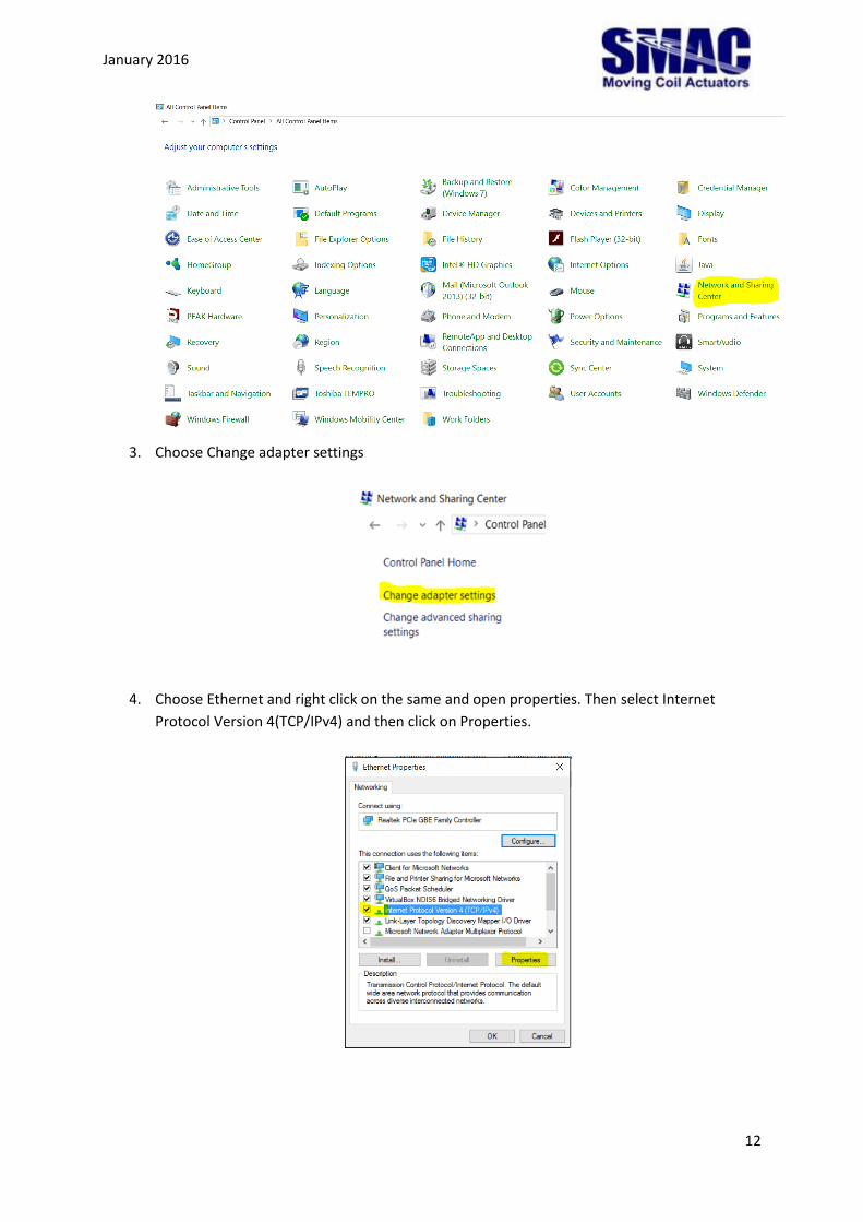
2.3.2.2 LAN-Setup
1. Open control panel
2. Choose Network and Sharing Center
+ -
24 VDC, 2 A supply
January 2016
12
3. Choose Change adapter settings
4. Choose Ethernet and right click on the same and open properties. Then select Internet
Protocol Version 4(TCP/IPv4) and then click on Properties.
January 2016
13
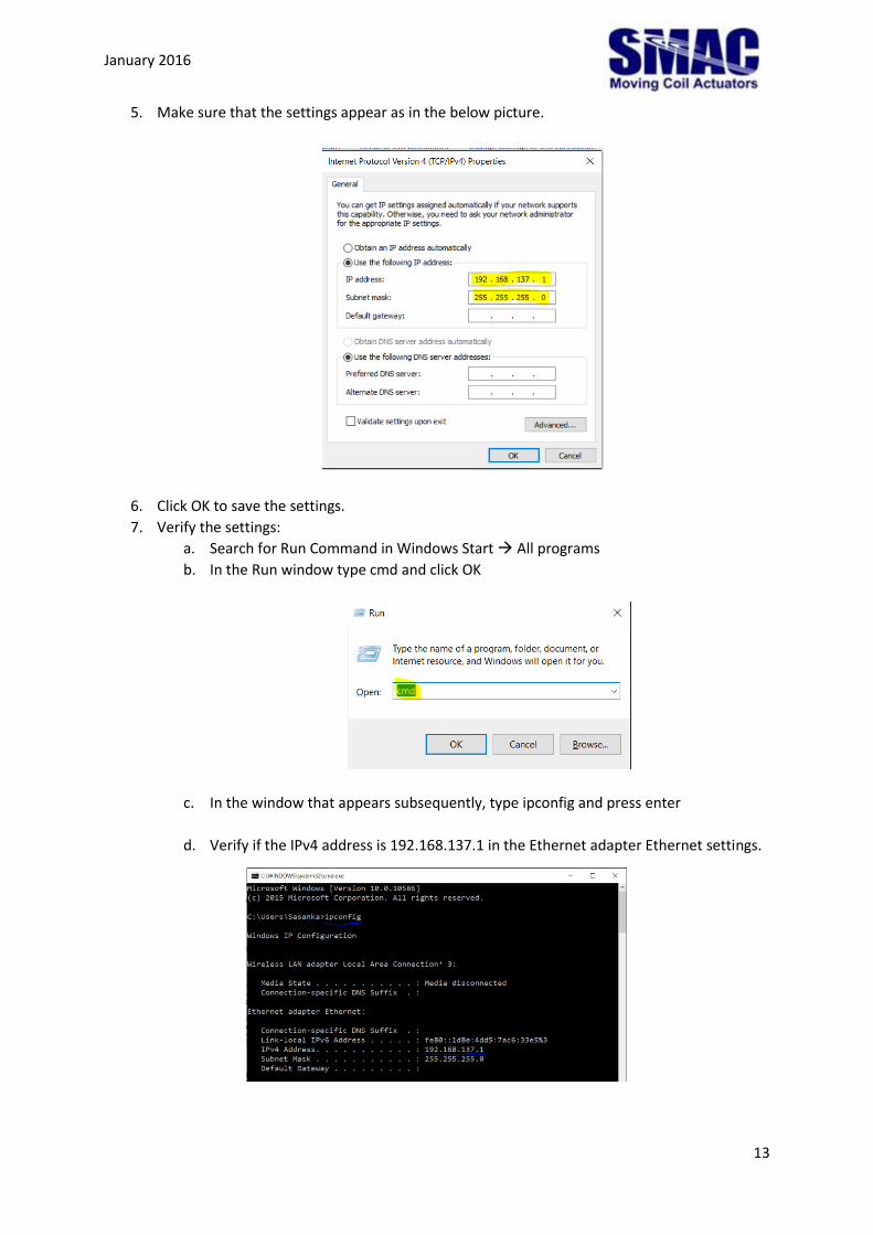
5. Make sure that the settings appear as in the below picture.
6. Click OK to save the settings.
7. Verify the settings:
a. Search for Run Command in Windows Start All programs
b. In the Run window type cmd and click OK
c. In the window that appears subsequently, type ipconfig and press enter
d. Verify if the IPv4 address is 192.168.137.1 in the Ethernet adapter Ethernet settings.
January 2016
14
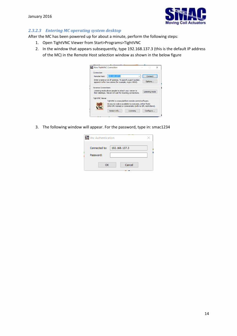
2.3.2.3 Entering MC operating system desktop
After the MC has been powered up for about a minute, perform the following steps:
1. Open TightVNC Viewer from Start>Programs>TightVNC
2. In the window that appears subsequently, type 192.168.137.3 (this is the default IP address
of the MC) in the Remote Host selection window as shown in the below figure
3. The following window will appear. For the password, type in: smac1234
January 2016
15
Navigating through the MC operating system
3.1 Configuring the MC firmware
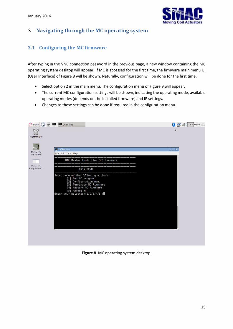
After typing in the VNC connection password in the previous page, a new window containing the MC
operating system desktop will appear. If MC is accessed for the first time, the firmware main menu UI
(User Interface) of Figure 8 will be shown. Naturally, configuration will be done for the first time.
Select option 2 in the main menu. The configuration menu of Figure 9 will appear.
The current MC configuration settings will be shown, indicating the operating mode, available
operating modes (depends on the installed firmware) and IP settings.
Changes to these settings can be done if required in the configuration menu.
Figure 8. MC operating system desktop.
January 2016
16
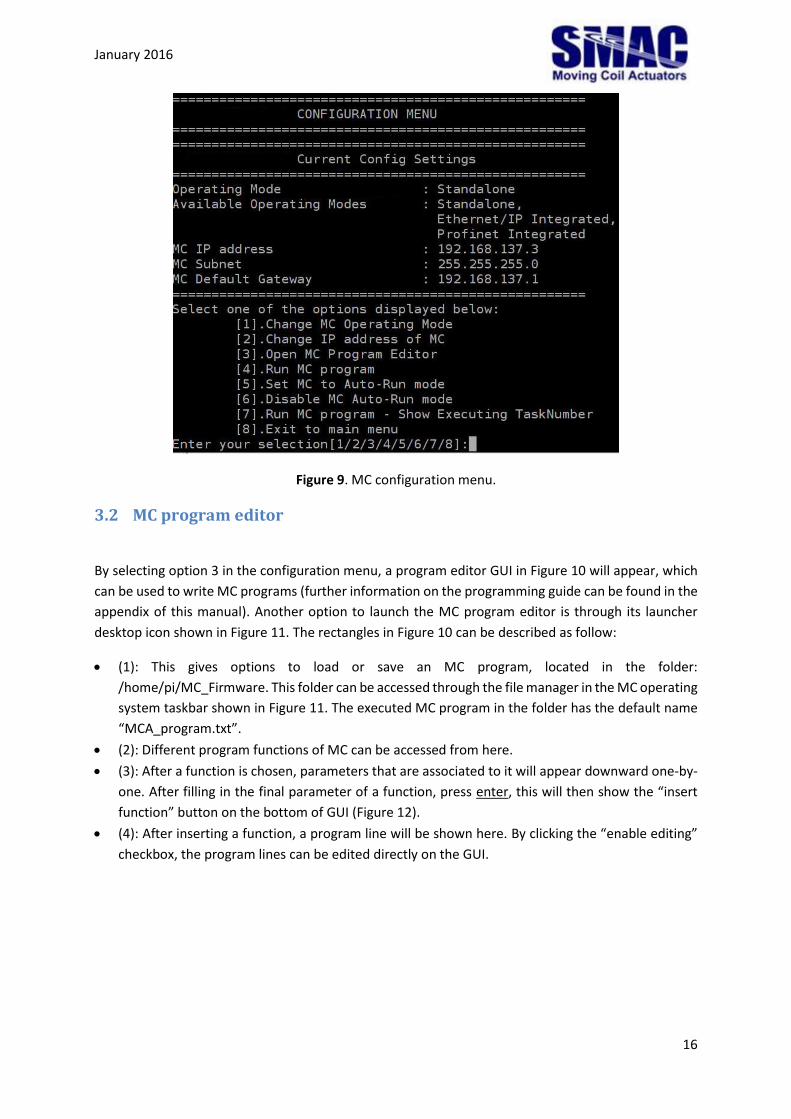
Figure 9. MC configuration menu.
3.2 MC program editor
By selecting option 3 in the configuration menu, a program editor GUI in Figure 10 will appear, which
can be used to write MC programs (further information on the programming guide can be found in the
appendix of this manual). Another option to launch the MC program editor is through its launcher
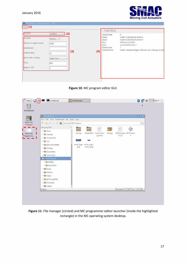
desktop icon shown in Figure 11. The rectangles in Figure 10 can be described as follow:
(1): This gives options to load or save an MC program, located in the folder:
/home/pi/MC_Firmware. This folder can be accessed through the file manager in the MC operating
system taskbar shown in Figure 11. The executed MC program in the folder has the default name
“MCA_program.txt”.
(2): Different program functions of MC can be accessed from here.
(3): After a function is chosen, parameters that are associated to it will appear downward one-by-
one. After filling in the final parameter of a function, press enter, this will then show the “insert
function” button on the bottom of GUI (Figure 12).
(4): After inserting a function, a program line will be shown here. By clicking the “enable editing”
checkbox, the program lines can be edited directly on the GUI.
January 2016
17
Figure 10. MC program editor GUI.
Figure 11. File manager (circled) and MC programmer editor launcher (inside the highlighted
rectangle) in the MC operating system desktop.
(1)
(2)
(3) (4)
January 2016
18
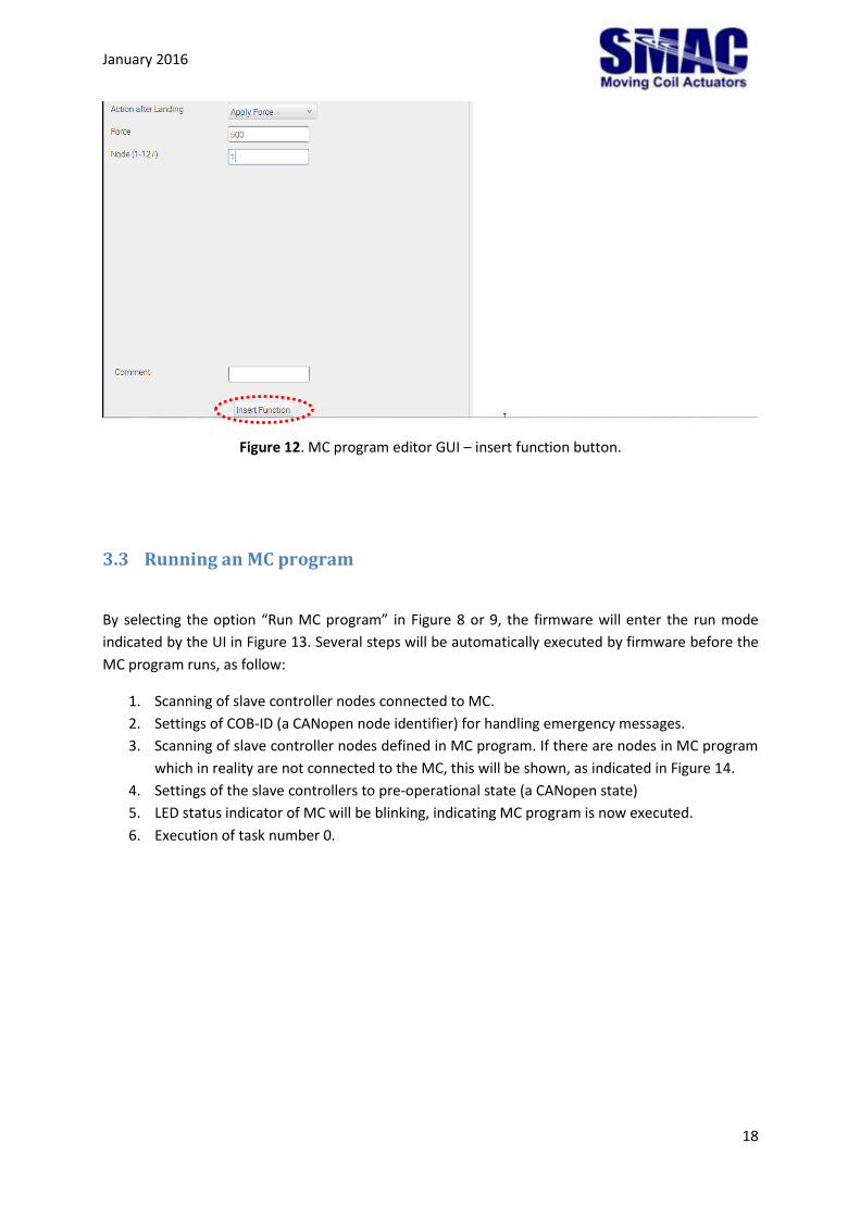
Figure 12. MC program editor GUI – insert function button.
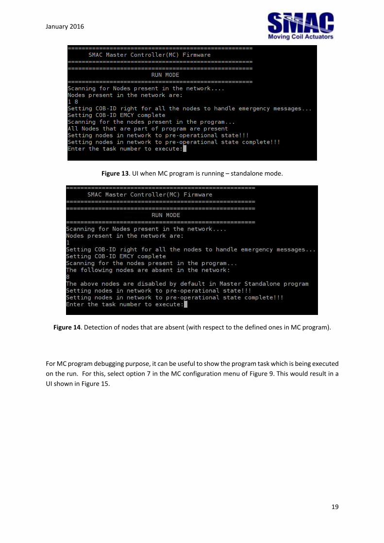
3.3 Running an MC program
By selecting the option “Run MC program” in Figure 8 or 9, the firmware will enter the run mode
indicated by the UI in Figure 13. Several steps will be automatically executed by firmware before the
MC program runs, as follow:
1. Scanning of slave controller nodes connected to MC.
2. Settings of COB-ID (a CANopen node identifier) for handling emergency messages.
3. Scanning of slave controller nodes defined in MC program. If there are nodes in MC program
which in reality are not connected to the MC, this will be shown, as indicated in Figure 14.
4. Settings of the slave controllers to pre-operational state (a CANopen state)
5. LED status indicator of MC will be blinking, indicating MC program is now executed.
6. Execution of task number 0.
January 2016
19
Figure 13. UI when MC program is running – standalone mode.
Figure 14. Detection of nodes that are absent (with respect to the defined ones in MC program).
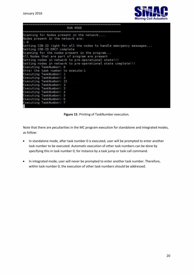
For MC program debugging purpose, it can be useful to show the program task which is being executed
on the run. For this, select option 7 in the MC configuration menu of Figure 9. This would result in a
UI shown in Figure 15.
January 2016
20
Figure 15. Printing of TaskNumber execution.
Note that there are peculiarities in the MC program execution for standalone and integrated modes,
as follow:
In standalone mode, after task number 0 is executed, user will be prompted to enter another
task number to be executed. Automatic execution of other task numbers can be done by
specifying this in task number 0, for instance by a task jump or task call command.
In integrated mode, user will never be prompted to enter another task number. Therefore,
within task number 0, the execution of other task numbers should be addressed.

January 2016
21
Figure 16. UI when MC program is running – integrated Ethernet/IP mode.
3.4 Terminating a running MC program
To terminate a running program, simply press Ctrl+C in the UI of run mode. Afterwards, the main
menu of Figure 8 will be shown.
January 2016
22
Tutorial
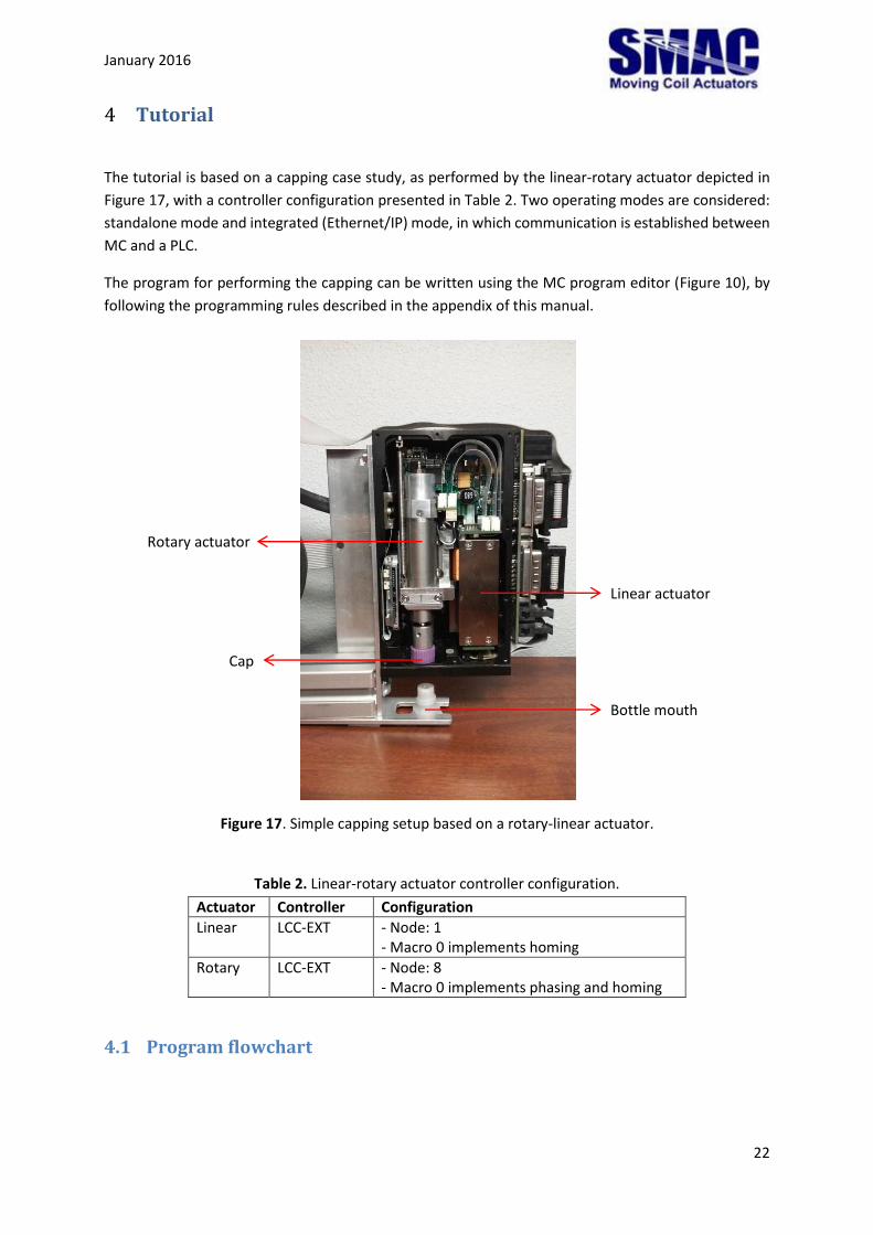
The tutorial is based on a capping case study, as performed by the linear-rotary actuator depicted in
Figure 17, with a controller configuration presented in Table 2. Two operating modes are considered:
standalone mode and integrated (Ethernet/IP) mode, in which communication is established between
MC and a PLC.
The program for performing the capping can be written using the MC program editor (Figure 10), by
following the programming rules described in the appendix of this manual.
Figure 17. Simple capping setup based on a rotary-linear actuator.
Table 2. Linear-rotary actuator controller configuration.
Actuator Controller Configuration
Linear LCC-EXT - Node: 1 - Macro 0 implements homing
Rotary LCC-EXT - Node: 8 - Macro 0 implements phasing and homing
4.1 Program flowchart
Bottle mouth
Linear actuator
Cap
Rotary actuator
January 2016
23
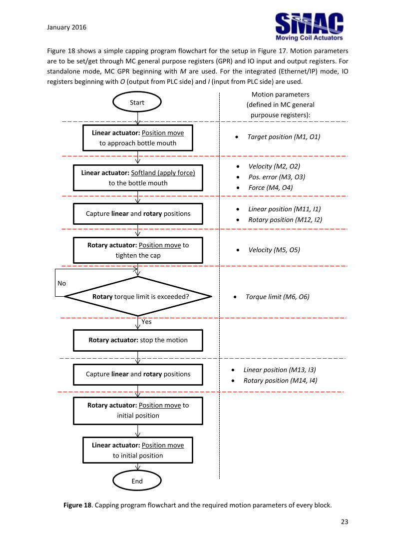
Figure 18 shows a simple capping program flowchart for the setup in Figure 17. Motion parameters
are to be set/get through MC general purpose registers (GPR) and IO input and output registers. For
standalone mode, MC GPR beginning with M are used. For the integrated (Ethernet/IP) mode, IO
registers beginning with O (output from PLC side) and I (input from PLC side) are used.
Figure 18. Capping program flowchart and the required motion parameters of every block.
Linear position (M13, I3)
Rotary position (M14, I4)
Linear position (M11, I1)
Rotary position (M12, I2)
Target position (M1, O1)
Torque limit (M6, O6)
Velocity (M5, O5)
Velocity (M2, O2)
Pos. error (M3, O3)
Force (M4, O4)
No
Yes
Start
Linear actuator: Position move
to approach bottle mouth
Linear actuator: Softland (apply force)
to the bottle mouth
Rotary actuator: Position move to
tighten the cap
Rotary torque limit is exceeded?
Rotary actuator: stop the motion
Rotary actuator: Position move to
initial position
Linear actuator: Position move
to initial position
End
Motion parameters
(defined in MC general
purpouse registers):
Capture linear and rotary positions
Capture linear and rotary positions
January 2016
24
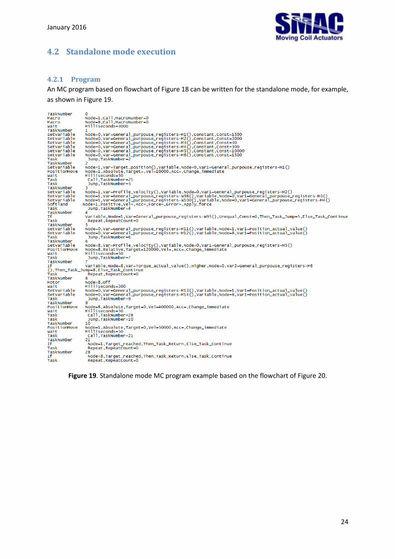
4.2 Standalone mode execution
4.2.1 Program
An MC program based on flowchart of Figure 18 can be written for the standalone mode, for example,
as shown in Figure 19.
Figure 19. Standalone mode MC program example based on the flowchart of Figure 20.
January 2016
25
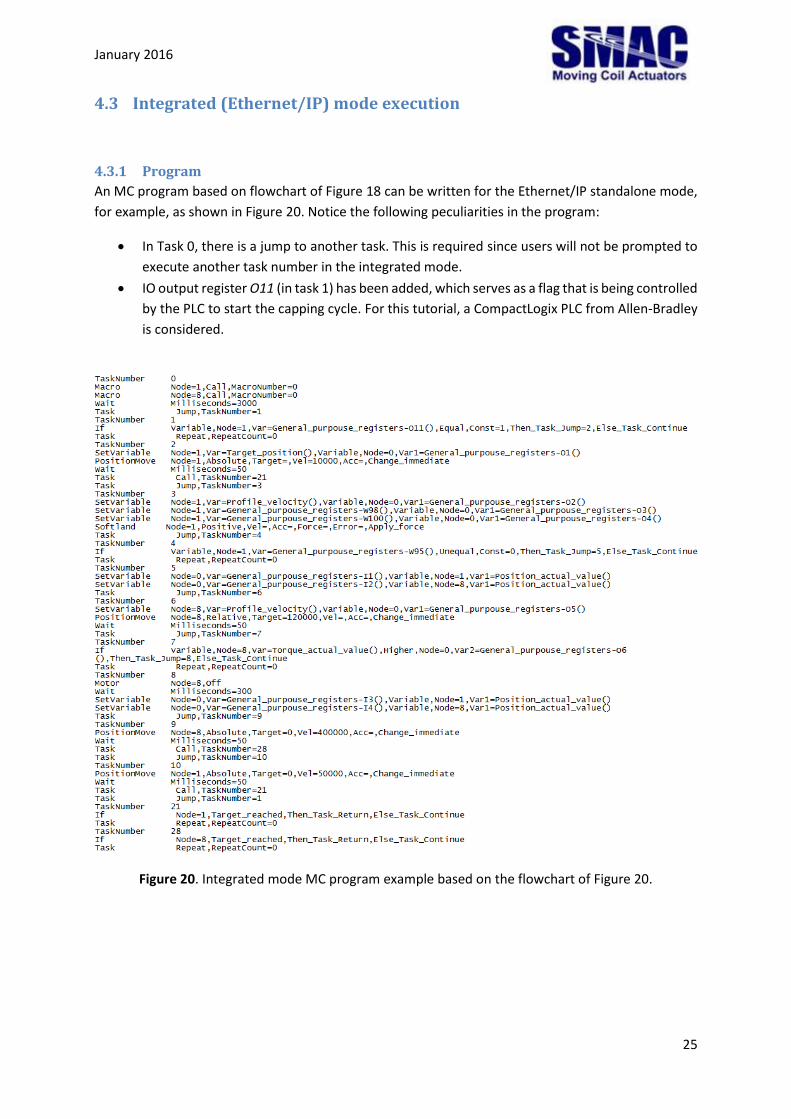
4.3 Integrated (Ethernet/IP) mode execution
4.3.1 Program
An MC program based on flowchart of Figure 18 can be written for the Ethernet/IP standalone mode,
for example, as shown in Figure 20. Notice the following peculiarities in the program:
In Task 0, there is a jump to another task. This is required since users will not be prompted to
execute another task number in the integrated mode.
IO output register O11 (in task 1) has been added, which serves as a flag that is being controlled
by the PLC to start the capping cycle. For this tutorial, a CompactLogix PLC from Allen-Bradley
is considered.
Figure 20. Integrated mode MC program example based on the flowchart of Figure 20.

January 2016
26
4.3.2 EDS file installation for Allen-Bradley PLCs
The EDS (Electronic Datasheet) file contains Ethernet/IP parameters such as device information,
number of inputs/outputs, datatypes, etc., which can be used to configure the communication
between the PLC and MC. The MC has an embedded EDS file in it, which can be uploaded using the
RSLinx Classic software as follow:
1. Make a physical connection between the MC, PLC and PC (with the RSLinx Classic software
opened) using Ethernet cables. Turn on the MC and PLC.
2. Make sure that MC is set to Ethernet/IP Run Mode as indicated in Figure 16.
3. In the RSLinx Classic software environment (Figure 21), go to the tab and select
Communications>Configure Drivers.
4. Select Ethernet/IP Driver from the Available Driver Types, add it to the list of Configured
Drivers. Next, select the Ethernet adapter belonging to the PC.
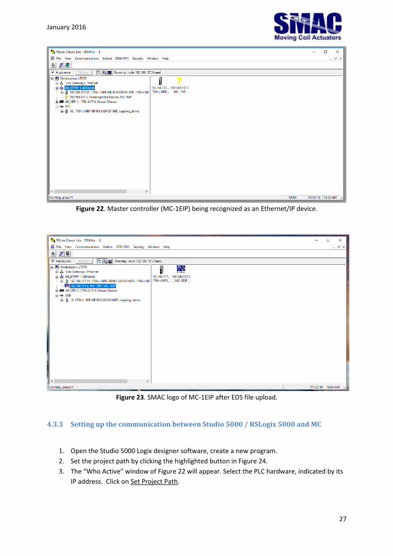
5. Click on the newly added Ethernet/IP driver on the left-hand side of the window in Figure 22.
This will show the master controller (shown as MC-1EIP) with a question mark logo.
6. Right-click on the MC-1EIP, and select “upload EDS file from the device”. Go through the steps
of uploading the file. Afterwards, the question mark logo will change to a SMAC logo (Figure
23), indicating that the EDS file has been uploaded.
Figure 21. Driver Configuration in RSLinx Classic.
January 2016
27
Figure 22. Master controller (MC-1EIP) being recognized as an Ethernet/IP device.
Figure 23. SMAC logo of MC-1EIP after EDS file upload.
4.3.3 Setting up the communication between Studio 5000 / RSLogix 5000 and MC
1. Open the Studio 5000 Logix designer software, create a new program.
2. Set the project path by clicking the highlighted button in Figure 24.
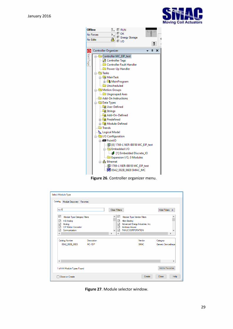
3. The “Who Active” window of Figure 22 will appear. Select the PLC hardware, indicated by its
IP address. Click on Set Project Path.
January 2016
28
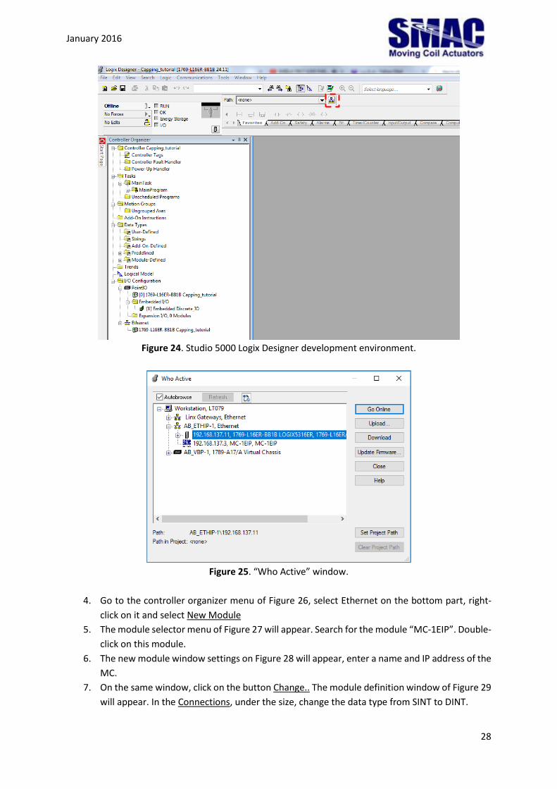
Figure 24. Studio 5000 Logix Designer development environment.
Figure 25. “Who Active” window.
4. Go to the controller organizer menu of Figure 26, select Ethernet on the bottom part, right-
click on it and select New Module
5. The module selector menu of Figure 27 will appear. Search for the module “MC-1EIP”. Double-
click on this module.
6. The new module window settings on Figure 28 will appear, enter a name and IP address of the
MC.
7. On the same window, click on the button Change.. The module definition window of Figure 29
will appear. In the Connections, under the size, change the data type from SINT to DINT.
January 2016
29
Figure 26. Controller organizer menu.
Figure 27. Module selector window.
January 2016
30
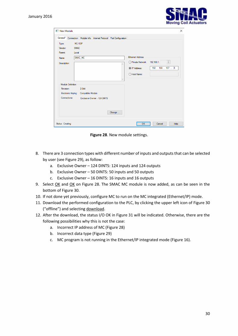
Figure 28. New module settings.
8. There are 3 connection types with different number of inputs and outputs that can be selected
by user (see Figure 29), as follow:
a. Exclusive Owner – 124 DINTS: 124 inputs and 124 outputs
b. Exclusive Owner – 50 DINTS: 50 inputs and 50 outputs
c. Exclusive Owner – 16 DINTS: 16 inputs and 16 outputs
9. Select OK and OK on Figure 28. The SMAC MC module is now added, as can be seen in the
bottom of Figure 30.
10. If not done yet previously, configure MC to run on the MC integrated (Ethernet/IP) mode.
11. Download the performed configuration to the PLC, by clicking the upper left icon of Figure 30
(“offline”) and selecting download.
12. After the download, the status I/O OK in Figure 31 will be indicated. Otherwise, there are the
following possibilities why this is not the case:
a. Incorrect IP address of MC (Figure 28)
b. Incorrect data type (Figure 29)
c. MC program is not running in the Ethernet/IP integrated mode (Figure 16).

January 2016
31
Figure 29. Module definition.
Figure 30. SMAC MC module is now added.

January 2016
32
Figure 31. I/O OK: an indication that Ethernet/IP communication between PLC and MC has been
successfully established.
January 2016
33
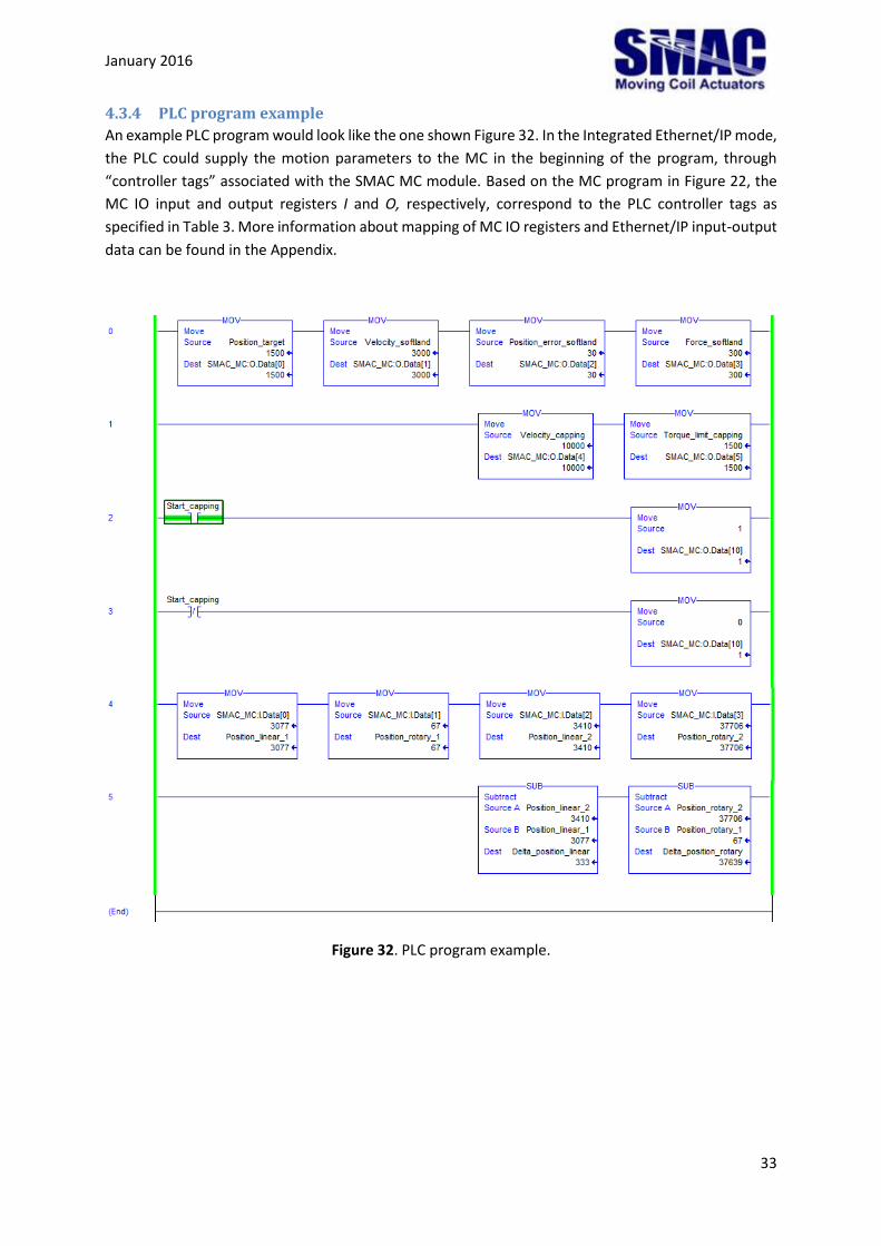
4.3.4 PLC program example
An example PLC program would look like the one shown Figure 32. In the Integrated Ethernet/IP mode,
the PLC could supply the motion parameters to the MC in the beginning of the program, through
“controller tags” associated with the SMAC MC module. Based on the MC program in Figure 22, the
MC IO input and output registers I and O, respectively, correspond to the PLC controller tags as
specified in Table 3. More information about mapping of MC IO registers and Ethernet/IP input-output
data can be found in the Appendix.
Figure 32. PLC program example.
January 2016
34
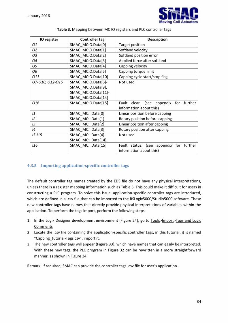
Table 3. Mapping between MC IO registers and PLC controller tags
IO register Controller tag Description
O1 SMAC_MC:O.Data[0] Target position
O2 SMAC_MC:O.Data[1] Softland velocity
O3 SMAC_MC:O.Data[2] Softland position error
O4 SMAC_MC:O.Data[3] Applied force after softland
O5 SMAC_MC:O.Data[4] Capping velocity
O6 SMAC_MC:O.Data[5] Capping torque limit
O11 SMAC_MC:O.Data[10] Capping cycle start/stop flag
O7-O10, O12-O15 SMAC_MC:O.Data[6]- SMAC_MC:O.Data[9], SMAC_MC:O.Data[11]- SMAC_MC:O.Data[14]
Not used
O16 SMAC_MC:O.Data[15] Fault clear. (see appendix for further information about this)
I1 SMAC_MC:I.Data[0] Linear position before capping
I2 SMAC_MC:I.Data[1] Rotary position before capping
I3 SMAC_MC:I.Data[2] Linear position after capping
I4 SMAC_MC:I.Data[3] Rotary position after capping
I5-I15 SMAC_MC:I.Data[4]- SMAC_MC:I.Data[14],
Not used
I16 SMAC_MC:I.Data[15] Fault status. (see appendix for further information about this)
4.3.5 Importing application-specific controller tags
The default controller tag names created by the EDS file do not have any physical interpretations,
unless there is a register mapping information such as Table 3. This could make it difficult for users in
constructing a PLC program. To solve this issue, application-specific controller tags are introduced,
which are defined in a .csv file that can be imported to the RSLogix5000/Studio5000 software. These
new controller tags have names that directly provide physical interpretations of variables within the
application. To perform the tags import, perform the following steps:
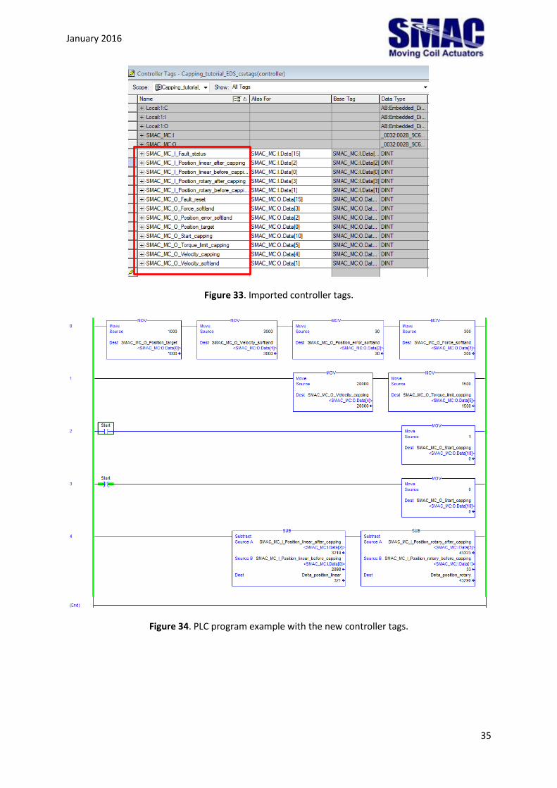
1. In the Logix Designer development environment (Figure 24), go to Tools>Import>Tags and Logic
Comments
2. Locate the .csv file containing the application-specific controller tags, in this tutorial, it is named
“Capping_tutorial-Tags.csv”, import it.
3. The new controller tags will appear (Figure 33), which have names that can easily be interpreted.
With these new tags, the PLC program in Figure 32 can be rewritten in a more straightforward
manner, as shown in Figure 34.
Remark: If required, SMAC can provide the controller tags .csv file for user’s application.
January 2016
35
Figure 33. Imported controller tags.
Figure 34. PLC program example with the new controller tags.
January 2016
36
Appendix: Programming the master controller
Program structure
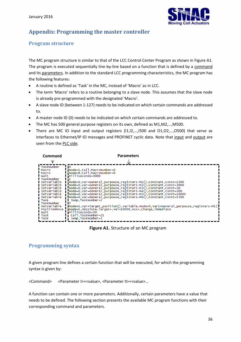
The MC program structure is similar to that of the LCC Control Center Program as shown in Figure A1.
The program is executed sequentially line-by-line based on a function that is defined by a command
and its parameters. In addition to the standard LCC programming characteristics, the MC program has
the following features:
A routine is defined as ‘Task’ in the MC, instead of ‘Macro’ as in LCC.
The term ‘Macro’ refers to a routine belonging to a slave node. This assumes that the slave node
is already pre-programmed with the designated ‘Macro’.
A slave node ID (between 1-127) needs to be indicated on which certain commands are addressed
to.
A master node ID (0) needs to be indicated on which certain commands are addressed to.
The MC has 500 general purpose registers on its own, defined as M1,M2,…,M500.
There are MC IO input and output registers (I1,I2,…,I500 and O1,O2,…,O500) that serve as
interfaces to Ethernet/IP IO messages and PROFINET cyclic data. Note that input and output are
seen from the PLC side.
Figure A1. Structure of an MC program
Programming syntax
A given program line defines a certain function that will be executed, for which the programming
syntax is given by:
<Command> <Parameter I>=<value>, <Parameter II>=<value>…
A function can contain one or more parameters. Additionally, certain parameters have a value that
needs to be defined. The following section presents the available MC program functions with their
corresponding command and parameters.
Command Parameters
January 2016
37
Function list
Task number (command: TaskNumber)
o Description:
Defines the task number, after which the subsequent functions are executed up to a new
definition of a task number.
o Parameter:
I. An integer
o Programming example:
TaskNumber 10
Task (command: Task)
o Description:
Defines the action performed on a certain task
o Parameters:
I. Action: Jump, Call, Repeat, Return
II. TaskNumber=<an integer>, RepeatCount=<no. of repetition>
TaskNumber: is added when Jump and Call are used
<an integer>: refers to a defined task number in the program
RepeatCount: is added when Repeat is used
<no. of repetition>: Number of repetition of the task repeat
o Programming example:
Task Jump,TaskNumber=1
Macro call (command: Macro)
o Description:
Provides access to a macro of a slave controller
o Parameter:
I. Node=<node number>
Node number ranges from 1-127
II. Action: Call
III. MacroNumber=<an integer>
<an integer>: refers to a macro number defined in the slave controller
o Programming example:
Macro Node=33,Call,MacroNumber=2
Get variable (command: GetVariable)
o Description:
Get the value of a certain variable and show it on the terminal window while program is
running.
o Parameter:
I. Node=<node number>
Node number ranges from 0-127
January 2016
38
Note that Node 0 refers to MC and only registers that are associated to it are
accessible.
II. Variable to get: Var=<a variable>
<a variable>: refers to an object defined in the emcl manual, as well as the MC
general purpose registers M1, M2,…, M500 and MC industrial ethernet interface
input and output registers I1, I2, … and O1, O2, ….
See the variable list in the end of this document.
o Programming example:
GetVariable Node=33,Var=Position_actual_value()
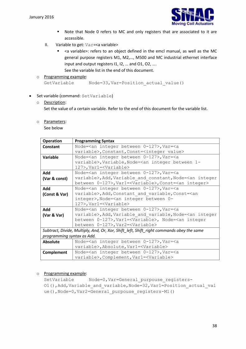
Set variable (command: SetVariable)
o Description:
Set the value of a certain variable. Refer to the end of this document for the variable list.
o Parameters:
See below
Operation Programming Syntax
Constant Node=<an integer between 0-127>,Var=<a
variable>,Constant,Const=<integer value>
Variable Node=<an integer between 0-127>,Var=<a
variable>,Variable,Node=<an integer between 1-
127>,Var1=<Variable>
Add (Var & const)
Node=<an integer between 0-127>,Var=<a
variable>,Add,Variable_and_constant,Node=<an integer
between 0-127>,Var1=<Variable>,Const=<an integer>
Add (Const & Var)
Node=<an integer between 0-127>,Var=<a
variable>,Add,Constant_and_variable,Const=<an
integer>,Node=<an integer between 0-
127>,Var1=<Variable>
Add (Var & Var)
Node=<an integer between 0-127>,Var=<a
variable>,Add,Variable_and_variable,Node=<an integer
between 0-127>,Var1=<Variable>, Node=<an integer
between 0-127>,Var2=<Variable>
Subtract, Divide, Multiply, And, Or, Xor, Shift_left, Shift_right commands obey the same programming syntax as Add.
Absolute Node=<an integer between 0-127>,Var=<a
variable>,Absolute,Var1=<Variable>
Complement Node=<an integer between 0-127>,Var=<a
variable>,Complement,Var1=<Variable>
o Programming example:
SetVariable Node=0,Var=General_purpouse_registers-
O1(),Add,Variable_and_variable,Node=32,Var1=Position_actual_val
ue(),Node=0,Var2=General_purpouse_registers-M1()
January 2016
39
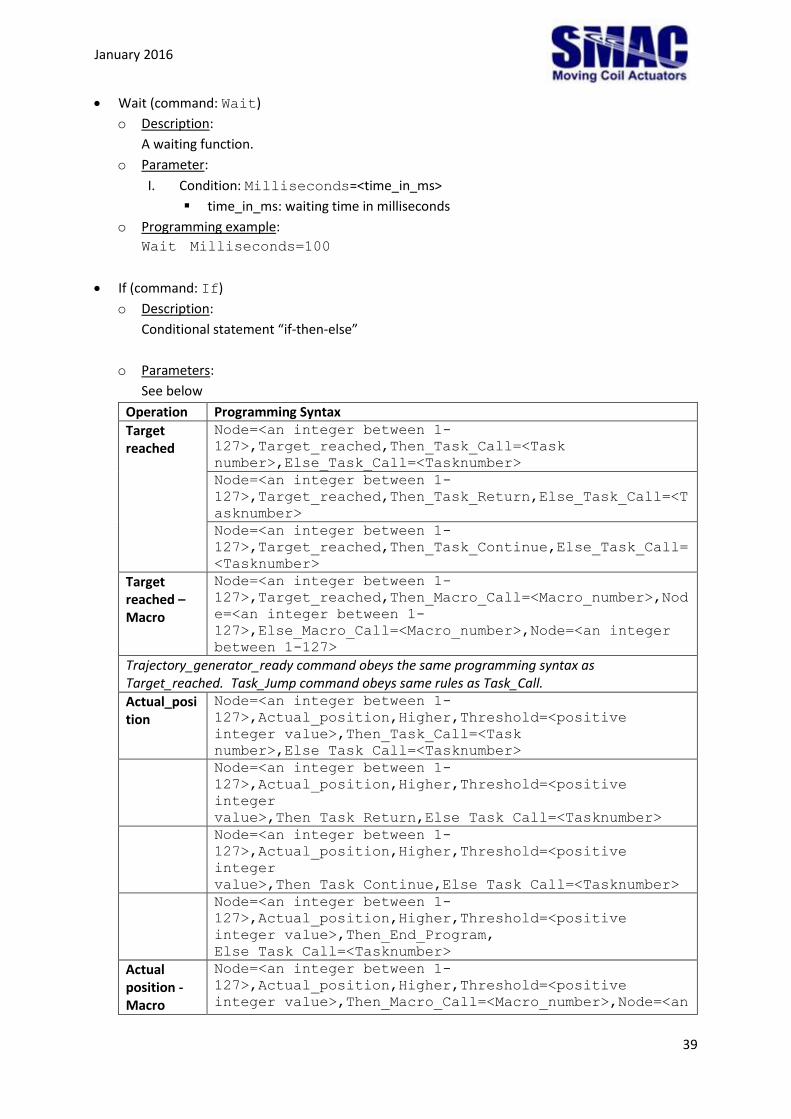
Wait (command: Wait)
o Description:
A waiting function.
o Parameter:
I. Condition: Milliseconds=<time_in_ms>
time_in_ms: waiting time in milliseconds
o Programming example:
Wait Milliseconds=100
If (command: If)
o Description:
Conditional statement “if-then-else”
o Parameters:
See below
Operation Programming Syntax
Target reached
Node=<an integer between 1-
127>,Target_reached,Then_Task_Call=<Task
number>,Else_Task_Call=<Tasknumber>
Node=<an integer between 1-
127>,Target_reached,Then_Task_Return,Else_Task_Call=<T
asknumber>
Node=<an integer between 1-
127>,Target_reached,Then_Task_Continue,Else_Task_Call=
<Tasknumber>
Target reached – Macro
Node=<an integer between 1-
127>,Target_reached,Then_Macro_Call=<Macro_number>,Nod
e=<an integer between 1-
127>,Else_Macro_Call=<Macro_number>,Node=<an integer
between 1-127>
Trajectory_generator_ready command obeys the same programming syntax as Target_reached. Task_Jump command obeys same rules as Task_Call.
Actual_position
Node=<an integer between 1-
127>,Actual_position,Higher,Threshold=<positive
integer value>,Then_Task_Call=<Task
number>,Else_Task_Call=<Tasknumber>
Node=<an integer between 1-
127>,Actual_position,Higher,Threshold=<positive
integer
value>,Then_Task_Return,Else_Task_Call=<Tasknumber>
Node=<an integer between 1-
127>,Actual_position,Higher,Threshold=<positive
integer
value>,Then_Task_Continue,Else_Task_Call=<Tasknumber>
Node=<an integer between 1-
127>,Actual_position,Higher,Threshold=<positive
integer value>,Then_End_Program,
Else_Task_Call=<Tasknumber>
Actual position - Macro
Node=<an integer between 1-
127>,Actual_position,Higher,Threshold=<positive
integer value>,Then_Macro_Call=<Macro_number>,Node=<an

January 2016
40
integer between 1-
127>,Else_Macro_Call=<Macro_number>,Node=< an integer
between 1-127>
Actual_velocity, Actual_force, Actual_input_1, Actual_input_2 commands obey the same rule as Actual position. Higher/Lower are the allowed logical operations.
Digital_input_0
Node=<an integer between 1-
127>,Digital_input_0,On,Then_Task_Call=<Task
number>,Else_Task_Call=<Tasknumber>
Node=<an integer between 1-
127>,Digital_input_0,On,Then_Task_Return,Else_Task_Cal
l=<Tasknumber>
Node=<an integer between 1-
127>,Digital_input_0,On,Then_Task_Continue,Else_Task_C
all=<Tasknumber>
Node=<an integer between 1-
127>,Digital_input_0,On,Then_End_Program,
Else_Task_Call=<Tasknumber>
Digital_input_0 - Macro
Node=<an integer between 1-
127>,Digital_input_0,On,Then_Macro_Call=<Macro_number>
,Node=<an integer between 1-
127>,Else_Macro_Call=<Macro_number>,Node=<an integer
between 1-127>
Digital_input_1, Digital_input_2, Digital_input_3 obey the same programming Syntax. For Off: use Off instead of On.
Variable – Constant
Node=<an integer between 0-127>,
Variable,Higher,Const=<an
interger>,Then_Task_Call=<Task
number>,Else_Task_Call=<Tasknumber>
Node=<an integer between 0-127>,
Variable,Higher,Const=<an
integer>,Then_Task_Return,Else_Task_Call=<Tasknumber>
Node=<an integer between 0-127>,
Variable,Higher,Const=<an
integer>,Then_Task_Continue=<Task
number>,Else_Task_Call=<Tasknumber>
Node=<an integer between 0-127>,
Variable,Higher,Const=<an integer>,Then_End_Program,
Else_Task_Call=<Tasknumber>
Variable-Constant Macro
Node=<an integer between 0-127>,
Variable,Higher,Const=<an
integer>,Then_Macro_Call=<Macro_number>,Node=<an
integer between 1-
127>,Else_Macro_Call=<Macro_number>,Node=< an integer
between 1-127>
Allowed Logical operations are Higher,Lower,Equal and Unequal.
Variable – Variable
Node=<an integer between 0-127>,Variable,Higher,
Node=<an integer between 0-
127>,Var2=<Variable>,Then_Task_Call=<Task
number>,Else_Task_Call=<Tasknumber>
Node=<an integer between 0-127>, Variable,Higher,
Node=<an integer between 0-
127>,Var2=<Variable>,Then_Task_Return,Else_Task_Call=<
Tasknumber>
Node=<an integer between 0-127>,Variable,Higher,
Node=<an integer between 0-
January 2016
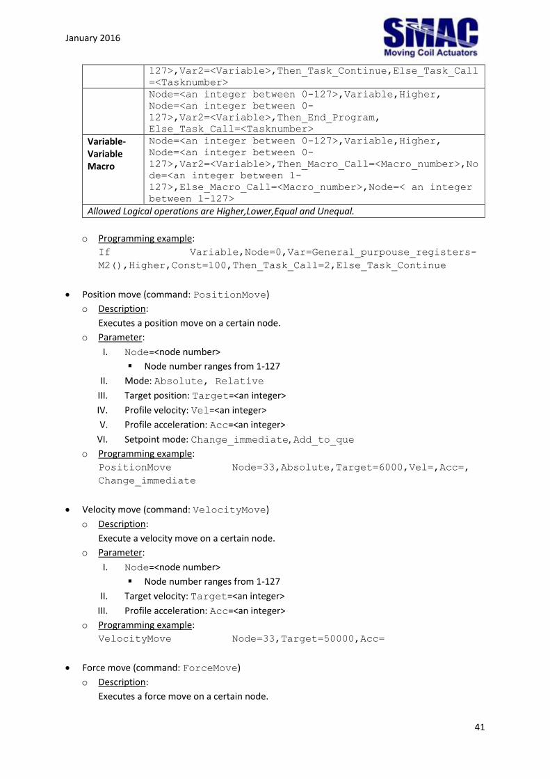
41
127>,Var2=<Variable>,Then_Task_Continue,Else_Task_Call
=<Tasknumber>
Node=<an integer between 0-127>,Variable,Higher,
Node=<an integer between 0-
127>,Var2=<Variable>,Then_End_Program,
Else_Task_Call=<Tasknumber>
Variable-Variable Macro
Node=<an integer between 0-127>,Variable,Higher,
Node=<an integer between 0-
127>,Var2=<Variable>,Then_Macro_Call=<Macro_number>,No
de=<an integer between 1-
127>,Else_Macro_Call=<Macro_number>,Node=< an integer
between 1-127>
Allowed Logical operations are Higher,Lower,Equal and Unequal.
o Programming example:
If Variable,Node=0,Var=General_purpouse_registers-
M2(),Higher,Const=100,Then_Task_Call=2,Else_Task_Continue
Position move (command: PositionMove)
o Description:
Executes a position move on a certain node.
o Parameter:
I. Node=<node number>
Node number ranges from 1-127
II. Mode: Absolute, Relative
III. Target position: Target=<an integer>
IV. Profile velocity: Vel=<an integer>
V. Profile acceleration: Acc=<an integer>
VI. Setpoint mode: Change_immediate, Add_to_que
o Programming example:
PositionMove Node=33,Absolute,Target=6000,Vel=,Acc=,
Change_immediate
Velocity move (command: VelocityMove)
o Description:
Execute a velocity move on a certain node.
o Parameter:
I. Node=<node number>
Node number ranges from 1-127
II. Target velocity: Target=<an integer>
III. Profile acceleration: Acc=<an integer>
o Programming example:
VelocityMove Node=33,Target=50000,Acc=
Force move (command: ForceMove)
o Description:
Executes a force move on a certain node.
January 2016
42
o Parameter:
I. Node=<node number>
Node number ranges from 1-127
II. Target force: Target=<an integer>
III. Profile slope: Slope=<an integer>
o Programming example:
ForceMove Node=23,Target=100,Slope=
Motor (command: Motor)
o Description:
Turns on/off motor
o Parameter:
I. Node=<node number>
Node number ranges from 1-127
II. Condition: On, Off
o Programming example:
Motor Node=32,Off
Set output (command: SetOutput)
o Description:
Sets the output value of a certain variable
o Parameter:
I. Node=<node number>
Node number ranges from 1-127
II. Output: Analog_output_10_bits=<an integer>,
Analog_output_16_bits=<an integer>,
Digital_output_0,On/Off, Digital_output_1,On/Off,
Digital_output_2,On/Off, Digital_output_3
o Programming example:
SetOutput Node=33,Digital_output_0,On
Homing (command: Homing)
o Description:
Executes a homing routine on a node
o Parameter:
I. Node=<node number>
II. Method: Endstop, Endstop_and_indexpulse, Indexpulse,
Use_current_position
If Endstop is used, parameter VII is not used
If Indexpulse is used, parameters V and VI are not used
If Use_current_position is used, parameters III – VIII are not used
III. Direction: Positive, Negative
IV. Acceleration: Acc=<an integer>
V. Velocity for endstop search: Vendstop=<an integer>
VI. Force for endstop detection: Force=<an integer>
January 2016
43
VII. Velocity for index search: Vindex=<an integer>
VIII. Timeout: Timeout=<an integer>
IX. Home offset: Offset=<an integer>
o Programming example:
Homing Node=32,Indexpulse,Positive,Acc=100,Vindex=50,
Timeout=1000,Offset=0
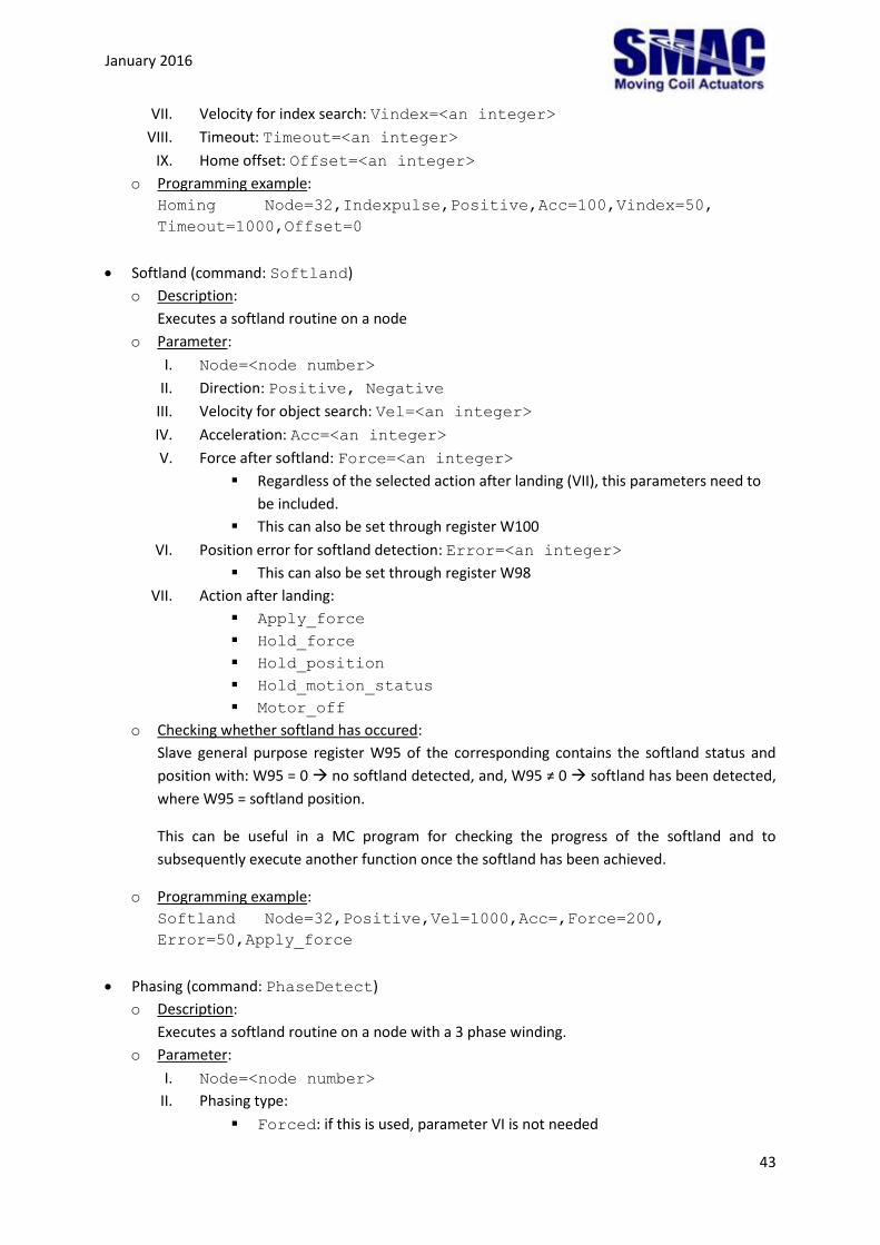
Softland (command: Softland)
o Description:
Executes a softland routine on a node
o Parameter:
I. Node=<node number>
II. Direction: Positive, Negative
III. Velocity for object search: Vel=<an integer>
IV. Acceleration: Acc=<an integer>
V. Force after softland: Force=<an integer>
Regardless of the selected action after landing (VII), this parameters need to
be included.
This can also be set through register W100
VI. Position error for softland detection: Error=<an integer>
This can also be set through register W98
VII. Action after landing:
Apply_force
Hold_force
Hold_position
Hold_motion_status
Motor_off
o Checking whether softland has occured:
Slave general purpose register W95 of the corresponding contains the softland status and
position with: W95 = 0 no softland detected, and, W95 ≠ 0 softland has been detected,
where W95 = softland position.
This can be useful in a MC program for checking the progress of the softland and to
subsequently execute another function once the softland has been achieved.
o Programming example:
Softland Node=32,Positive,Vel=1000,Acc=,Force=200,
Error=50,Apply_force
Phasing (command: PhaseDetect)
o Description:
Executes a softland routine on a node with a 3 phase winding.
o Parameter:
I. Node=<node number>
II. Phasing type:
Forced: if this is used, parameter VI is not needed
January 2016
44
Initial_position_allways_known: if this is used, parameters III – V
are skipped
III. Phasing time: Time=<an integer, in ms>
IV. Phasing current: Current=<an integer>
V. Phasing Tolerance: Tolerance=<an integer>
VI. Initial rotor position: Rotorpos=<an integer>
IO register – the bridge between MC and industrial Ethernet protocols
The IO input registers (I1 – I500) and output registers (O1 – O100) are MC program variables that are
mapped to data format are recognized by industrial ethrenet protocols (depending on the chosen
mode) discussed in this user manual, namely Ethernet/IP and PROFINET. The mapping of the variables
to the data are given in the following subsections.
IO register mapping for Ethernet/IP
The mapping between IO registers and Ethernet/IP IO data (as defined by EDS file in the tutorial section)
follows a numbering pattern shown in the Table A1. For a given EDS file, the last register in the inputs
and outputs refers to the fault status and fault clear, respectively. As an example, for an EDS file having
50 DINT input and 50 DINT outputs, the MC fault status is represented by I50 and SMAC_MC:I.Data[49].
Table A1. Mapping between IO registers and Ethernet/IP data – for 16 inputs and 16 outputs.
IO registers Ethernet/IP IO data Description
I1 SMAC_MC:I.Data[0] Input 1 (PLC side)
I2 SMAC_MC:I.Data[1] Input 2 (PLC side)
… … …
I16 SMAC_MC:I.Data[15] MC fault status
O1 SMAC_MC:O.Data[0] Output 1 (PLC side)
O2 SMAC_MC:O.Data[2] Output 2 (PLC side)
… … …
O16 SMAC_MC:O.Data[15] MC fault clear
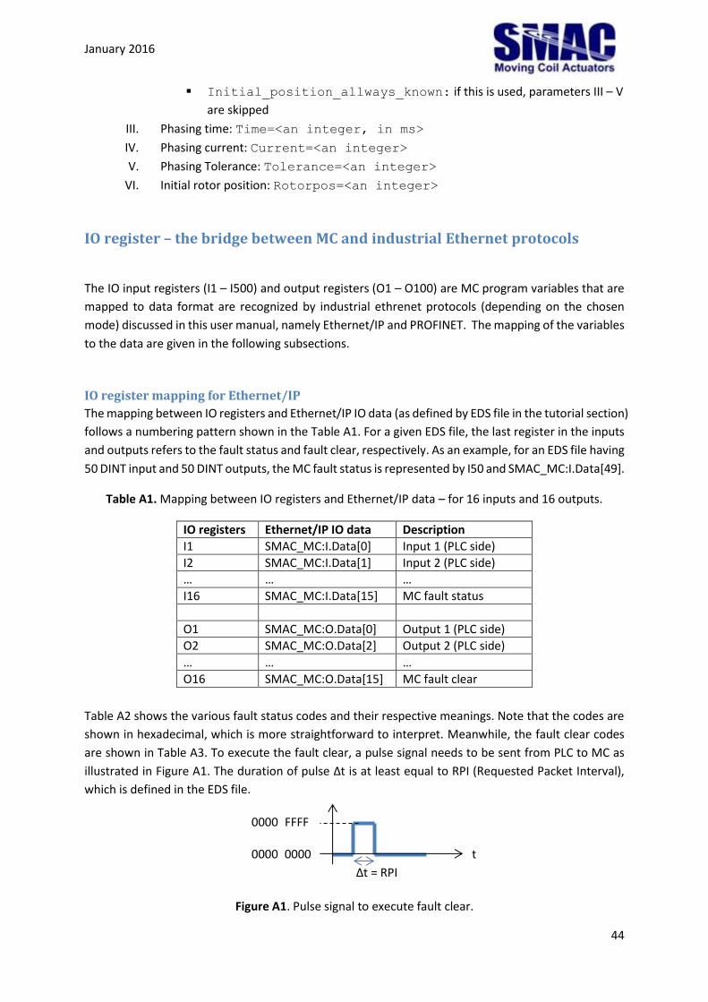
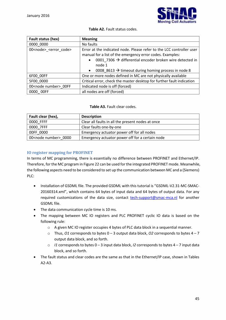
Table A2 shows the various fault status codes and their respective meanings. Note that the codes are
shown in hexadecimal, which is more straightforward to interpret. Meanwhile, the fault clear codes
are shown in Table A3. To execute the fault clear, a pulse signal needs to be sent from PLC to MC as
illustrated in Figure A1. The duration of pulse Δt is at least equal to RPI (Requested Packet Interval),
which is defined in the EDS file.
Figure A1. Pulse signal to execute fault clear.
0000_0000
0000_FFFF
t
Δt = RPI
January 2016
45
Table A2. Fault status codes.
Fault status (hex) Meaning
0000_0000 No faults
00<node>_<error_code> Error at the indicated node. Please refer to the LCC controller user manual for a list of the emergency error codes. Examples:
0001_7306 differential encoder broken wire detected in node 1
0008_8613 timeout during homing process in node 8
6F00_00FF One or more nodes defined in MC are not physically available
5F00_0000 Critical error, check the master desktop for further fault indication
00<node number>_00FF Indicated node is off (forced)
0000_ 00FF all nodes are off (forced)
Table A3. Fault clear codes.
Fault clear (hex), Description
0000_FFFF Clear all faults in all the present nodes at once
0000_7FFF Clear faults one-by-one
00FF_0000 Emergency actuator power off for all nodes
00<node number>_0000 Emergency actuator power off for a certain node
IO register mapping for PROFINET
In terms of MC programming, there is essentially no difference between PROFINET and Ethernet/IP.
Therefore, for the MC program in Figure 22 can be used for the integrated PROFINET mode. Meanwhile,
the following aspects need to be considered to set up the communication between MC and a (Siemens)
PLC:
Installation of GSDML file. The provided GSDML with this tutorial is “GSDML-V2.31-MC-SMAC-
20160314.xml”, which contains 64 bytes of input data and 64 bytes of output data. For any
required customizations of the data size, contact [email protected] for another
GSDML file.
The data communication cycle time is 10 ms.
The mapping between MC IO registers and PLC PROFINET cyclic IO data is based on the
following rule:
o A given MC IO register occupies 4 bytes of PLC data block in a sequential manner.
o Thus, O1 corresponds to bytes 0 – 3 output data block, O2 corresponds to bytes 4 – 7
output data block, and so forth.
o I1 corresponds to bytes 0 – 3 input data block, I2 corresponds to bytes 4 – 7 input data
block, and so forth.
The fault status and clear codes are the same as that in the Ethernet/IP case, shown in Tables
A2-A3.
January 2016
46
Variable list
The variables used in a MC program and their corresponding programming syntaxes are
presented in the table below. Further explanations about the variable/object characteristics
(functionalities, data types, etc.) can be found in the emcl library manual.
VARIABLE/OBJECT PROGRAMMING SYNTAX
UART configuration
Node ID Uart_configuration-Node_ID()
Baudrate Uart_configuration-Baudrate()
Daisy chain mode Uart_configuration-Daisy_chain_mode()
Base format Uart_configuration-Base_format()
Statusword mode Uart_configuration-Statusword_mode()
Phasing parameters
Phasing type Phasing-Phasing_type()
Phasing time Phasing-Phasing_time()
Phasing current Phasing-Phasing_current()
Phasing tolerance Phasing-Phasing_tolerance()
Phasing initial rotor position Phasing-Phasing_initial_rotor_position()
Phasing actual rotor position Phasing-Phasing_actual_rotor_position()
Homing parameters
Total homing timeout Homing_extra_parameters-
Total_homing_timeout()
Homing torque limit Homing_extra_parameters-Torque_limit()
Motor parameters
Motor pair poles Motor_pair_poles()
Position encoder swap mode Position_encoder_swap_mode()
Position encoder type Position_encoder_type()
System polarity System_polarity()
Command reference source Command_reference_source()
Step and direction command source
Step value Step_and_Direction_cmd_source-Step_value()
Analog input command source
Analog input used Analog_input_cmd_source-Analog_input_used()
Analog input offset Analog_input_cmd_source-
Analog_input_offset()
Velocity deadband Analog_input_cmd_source-Velocity_deadband()
Position control parameter set
Proportional constant Position_control_parameter_set-
Proportional_constant()
Integral constant Position_control_parameter_set-
Integral_constant()
Derivative constant Position_control_parameter_set-
Derivative_constant()
Velocity feedforward
constant
Position_control_parameter_set-
Velocity_feedforward_constant()
Acceleration feedforward
constant
Position_control_parameter_set-
Acceleration_feedforward_constant()
Integral limit Position_control_parameter_set-
Integral_limit()
January 2016
47
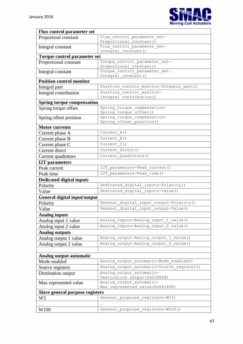
Flux control parameter set
Proportioal constant Flux_control_parameter_set-
Proportional_constant()
Integral constant Flux_control_parameter_set-
Integral_constant()
Torque control parameter set
Proportional constant Torque_control_parameter_set-
Proportional_constant()
Integral constant Torque_control_parameter_set-
Integral_constant()
Position control monitor
Integral part Position_control_monitor-Integral_part()
Integral contribution Position_control_monitor-
Integral_contribution()
Spring torque compensation
Spring torque offset Spring_torque_compensation-
Spring_torque_offset()
Spring offset position Spring_torque_compensation-
Spring_offset_position()
Motor currents
Current phase A Current_A()
Current phase B Current_B()
Current phase C Current_C()
Current direct Current_Direct()
Current quadrature Current_Quadrature()
I2T parameters
Peak current I2T_parameters-Peak_current()
Peak time I2T_parameters-Peak_time()
Dedicated digital inputs
Polarity Dedicated_digital_inputs-Polarity()
Value Dedicated_digital_inputs-Value()
General digital input/output
Polarity General_digital_input_output-Polarity()
Value General_digital_input_output-Value()
Analog inputs
Analog input 1 value Analog_inputs-Analog_input_1_value()
Analog input 2 value Analog_inputs-Analog_input_2_value()
Analog outputs
Analog output 1 value Analog_output-Analog_output_1_value()
Analog output 2 value Analog_output-Analog_output_2_value()
Analog output automatic
Mode enabled Analog_output_automatic-Mode_enabled()
Source registers Analog_output_automatic-Source_register()
Destination output Analog_output_automatic-
Destination_output(0x032A08)
Max represented value Analog_output_automatic-
Max_represented_value(0x042408)
Slave general purpose registers
W3 General_purpouse_registers-W3()
… …
W100 General_purpouse_registers-W100()

January 2016
48
Master general purpose registers
M1 General_purpouse_registers-M1()
M2 General_purpouse_registers-M2()
… …
M500 General_purpouse_registers-M500()
IO input registers
I1 General_purpouse_registers-I1()
I2 General_purpouse_registers-I2()
… …
I500 General_purpouse_registers-I500()
IO output registers
O1 General_purpouse_registers-O1()
O2 General_purpouse_registers-O2()
… …
O500 General_purpouse_registers-O500()
Learned position
Learn current position Learned_position-Learn_current_position()
Learn target position Learned_position-Learn_target_position()
Move index table position Learned_position-Move_index_table_position()
Macro commands
Macro call Macro_commands-Macro_call()
Return from macro call Macro_commands-Return_from_macro_call()
Macro jump Macro_commands-Macro_jump()
Reset macros Macro_commands-Reset_macros()
Jump absolute Macro_commands-Jump_absolute()
Jump relative Macro_commands-Jump_relative()
Unpush macro Macro_commands-Unpush_macro()
Timers access
Timer 1 (count up) value Timer_access-Timer_1_count_up_value()
Timer 2 (count up) value Timer_access-Timer_2_count_up_value()
Timer 3 (count down) value Timer_access-Timer_3_count_down_value()
Timer 4 (count down) value Timer_access-Timer_4_count_down_value()
Pointer access
Pointer to register Pointer_access-Pointer_to_register()
Content of register Pointer_access-Content_of_register()
Write content to register Pointer_access-Write_content_to_register()
Macro debug
Actual macro number Macro_debug-Actual_macro_number()
Actual command number Macro_debug-Actual_command_number()
Monitor config
Sampling rate Monitor_config-Sampling_rate()
Enable mode Monitor_config-Enable_mode()
Monitor result
Max. entry number Monitor_result-Max_entry_number()
Filled entry value Monitor_result-Filled_entry_values()
Entry number Monitor_result-Entry_number()
Actual entry table 1 Monitor_result-Actual_entry_table_1()
Actual entry table 2 Monitor_result-Actual_entry_table_2()
January 2016
49
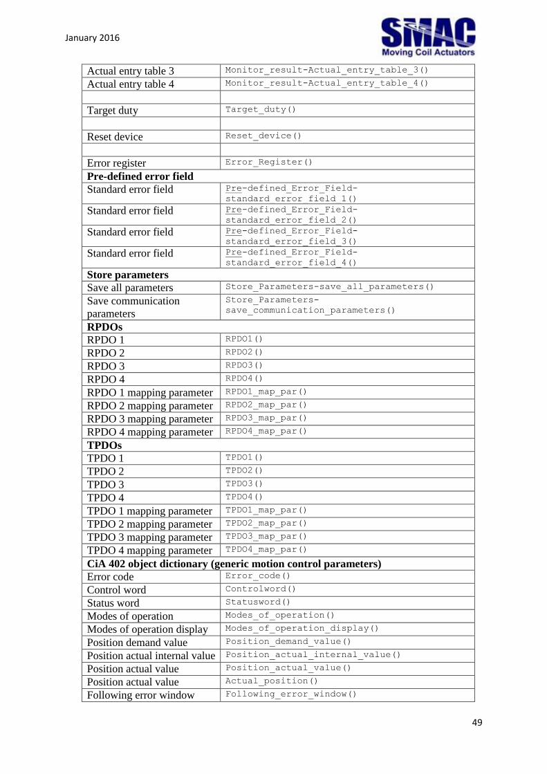
Actual entry table 3 Monitor_result-Actual_entry_table_3()
Actual entry table 4 Monitor_result-Actual_entry_table_4()
Target duty Target_duty()
Reset device Reset_device()
Error register Error_Register()
Pre-defined error field
Standard error field Pre-defined_Error_Field-
standard_error_field_1()
Standard error field Pre-defined_Error_Field-
standard_error_field_2()
Standard error field Pre-defined_Error_Field-
standard_error_field_3()
Standard error field Pre-defined_Error_Field-
standard_error_field_4()
Store parameters
Save all parameters Store_Parameters-save_all_parameters()
Save communication
parameters
Store_Parameters-
save_communication_parameters()
RPDOs
RPDO 1 RPDO1()
RPDO 2 RPDO2()
RPDO 3 RPDO3()
RPDO 4 RPDO4()
RPDO 1 mapping parameter RPDO1_map_par()
RPDO 2 mapping parameter RPDO2_map_par()
RPDO 3 mapping parameter RPDO3_map_par()
RPDO 4 mapping parameter RPDO4_map_par()
TPDOs
TPDO 1 TPDO1()
TPDO 2 TPDO2()
TPDO 3 TPDO3()
TPDO 4 TPDO4()
TPDO 1 mapping parameter TPDO1_map_par()
TPDO 2 mapping parameter TPDO2_map_par()
TPDO 3 mapping parameter TPDO3_map_par()
TPDO 4 mapping parameter TPDO4_map_par()
CiA 402 object dictionary (generic motion control parameters)
Error code Error_code()
Control word Controlword()
Status word Statusword()
Modes of operation Modes_of_operation()
Modes of operation display Modes_of_operation_display()
Position demand value Position_demand_value()
Position actual internal value Position_actual_internal_value()
Position actual value Position_actual_value()
Position actual value Actual_position()
Following error window Following_error_window()
January 2016
50
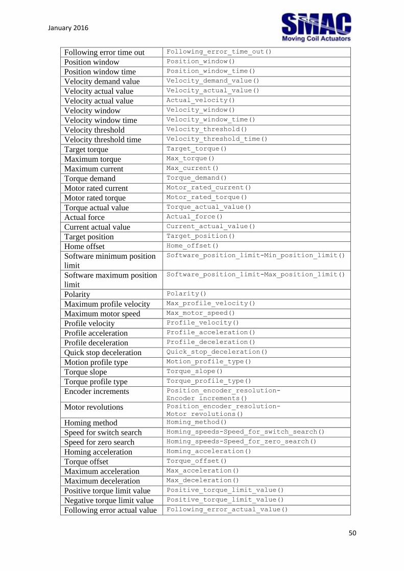
Following error time out Following_error_time_out()
Position window Position_window()
Position window time Position_window_time()
Velocity demand value Velocity_demand_value()
Velocity actual value Velocity_actual_value()
Velocity actual value Actual_velocity()
Velocity window Velocity_window()
Velocity window time Velocity_window_time()
Velocity threshold Velocity_threshold()
Velocity threshold time Velocity_threshold_time()
Target torque Target_torque()
Maximum torque Max_torque()
Maximum current Max_current()
Torque demand Torque_demand()
Motor rated current Motor_rated_current()
Motor rated torque Motor_rated_torque()
Torque actual value Torque_actual_value()
Actual force Actual_force()
Current actual value Current_actual_value()
Target position Target_position()
Home offset Home_offset()
Software minimum position
limit
Software_position_limit-Min_position_limit()
Software maximum position
limit
Software_position_limit-Max_position_limit()
Polarity Polarity()
Maximum profile velocity Max_profile_velocity()
Maximum motor speed Max_motor_speed()
Profile velocity Profile_velocity()
Profile acceleration Profile_acceleration()
Profile deceleration Profile_deceleration()
Quick stop deceleration Quick_stop_deceleration()
Motion profile type Motion_profile_type()
Torque slope Torque_slope()
Torque profile type Torque_profile_type()
Encoder increments Position_encoder_resolution-
Encoder_increments()
Motor revolutions Position_encoder_resolution-
Motor_revolutions()
Homing method Homing_method()
Speed for switch search Homing_speeds-Speed_for_switch_search()
Speed for zero search Homing_speeds-Speed_for_zero_search()
Homing acceleration Homing_acceleration()
Torque offset Torque_offset()
Maximum acceleration Max_acceleration()
Maximum deceleration Max_deceleration()
Positive torque limit value Positive_torque_limit_value()
Negative torque limit value Positive_torque_limit_value()
Following error actual value Following_error_actual_value()

January 2016
51
Control effort Control_effort()
Position demand internal
value
Position_demand_internal_value()
Target velocity Target_velocity()
Motor type Motor_type()
Supported drive mode Supported_Drive_mode()


![FLOW TEMP. CONTROLLER [MASTER] (Cased)](https://img.pdfslide.us/doc/110x75/61a5c558c919ca4ec446c173/flow-temp-controller-master-cased.jpg)